VeVaDaM Weather Radar in the Water Sector · VeVaDaM Weather Radar in the Water Sector ... Refshalevej 250 1432 København K ... The documentation gives a short overview of the needed

VeVaDaM Version 1.0

VeVaDaM Specifications - Logical and Physical Data Model Page 1 of 61

VeVaDaM

Weather Radar in the Water Sector

Logical and physical Data Model

Version Number: 1.0

Version Date: 29/03/2017

ABSTRACT

VeVaDaM is a data information model designed by the Danish water utility collaboration

VeVa (Weather radar in the Water sector). The intent of the data model is to make the

use and sharing of weather radar precipitation data easier for hydrological purposes. The

model represents the choices made by the VeVa collaboration and are inspired by the

OPERAs ODIM H5 (Michelson 2014).

The present document specifies the logical data model VeVaDaM and the physical

implementation in the file structure of VeVaDaM_H5. As the name implies the

implementation make use of the HDF5 file format developed and maintained by the HDF

Group (HDF-Group 2016).

The data model is constructed to be self-explanatory, give flexibility, transparency and

high usability for the end-user. The associated metadata and the required “best estimate”

of the precipitation field allows both general users and weather radar experts to directly

use the data in applications.

OVERBLIK (DANISH VERSION OF ABSTRACT)

VeVaDaM er en data information model udviklet af det danske vandforsynings

samarbejde VeVa (Vejrradar i Vandsektoren). Formålet med denne data informations

model er at gøre brugen og udvekslingen af vejrradar data nemmere for hydrologiske

formål. Modellen repræsenterer de valg VeVa partnerne har foretaget, og bygger videre

på OPERA’s ODIM H5 (Michelson 2014).

Dette dokument beskriver den logiske datamodel VeVaDaM og den tilhørende fysiske

data model VeVaDaM_H5 der som navnet antyder bygger på HDF5 fil strukturen (HDF-

Group 2016).

Datamodellen er konstrueret til at være selvforklarende, fleksibel, gennemsigtighed og

med høj anvendelig for slut brugerne. Den tilhørende meta-data information og det

krævede bedste bud på en areal nedbør gør det muligt både for generelle brugere og

vejrradar eksperter at anvende data eller arbejde videre med dem.

Specifikationerne er skrevet på engelsk for at gøre dem bredest muligt anvendelige.

VeVaDaM Version 1.0


VERSION HISTORY The responsibility and maintenance of this document lies with the VeVa partners.

The background for the VeVa collaboration and its partners are descripted further in

section 1.

Version 1.0, 29 Marts 2017

Final version approved by the VeVa partners.

Version 0.9, 17 February 2017

Draft final version for the VeVa partners review and scientific knowledge partners

(Aalborg University). This version was produced by InforMetics Aps and EnviDan A/S

on behalf of and in collaboration with the VeVa partners. The VeVaDaM specifications

are the results of multiple meetings and workshops with the purpose of clarifying the

VeVa partners needs and requirements of the data model.

VeVaDaM Version 1.0


TABLE OF CONTENTS

1 BACKGROUND AND VEVA PARTNERS ..................................................................... 5

2 INTRODUCTION ............................................................................................................... 7

2.1 PURPOSE ............................................................................................................ 7

2.2 RADAR DATA FLOW ....................................................................................... 7

2.3 GOVERNANCE .................................................................................................. 8

3 DATA MODEL CONCEPT ............................................................................................... 8

3.1 DEFINITIONS USED IN THE DATA MODEL ................................................ 9

3.1.1 Group .............................................................................................................. 9

3.1.2 Dataset............................................................................................................. 9

3.1.3 Attributes......................................................................................................... 9

3.1.4 Scalars, Booleans and Sequences ................................................................... 9

3.2 SCHEMATIZATION OF THE DATA MODEL ................................................ 9

3.2.1 Required data ................................................................................................ 11

3.2.2 Additional data .............................................................................................. 11

3.3 ASSUMPTIONS ................................................................................................ 12

3.4 INTERACTION WITH OTHER IT SYSTEMS ............................................... 12

3.5 LOGICAL DATA MODEL STANDARDS ...................................................... 13

4 META DATA DEFINITIONS ......................................................................................... 13

4.1 TEMPORAL STORAGE STRUCTURE ........................................................... 13

4.2 ROOT METADATA [REQUIRED] .................................................................. 14

4.3 DATA GROUP [REQUIRED] .......................................................................... 18

4.4 DATA, PRECIPITATION GROUP [REQUIRED] ........................................... 21

4.5 DATA, PRECIPITATIONADDITIONAL GROUP .......................................... 22

5 DATA SPECIFICATIONS .............................................................................................. 26

6 STANDARD AND ALTERNATIVE PROCESSES ...................................................... 28

6.1 CORRECTION OF RAW DATA ...................................................................... 29

6.1.1 Clutter and Noise reduction .......................................................................... 29

6.1.2 Attenuation correction .................................................................................. 31

6.1.3 Vertical Profile of Reflectivity (VPR) correction ......................................... 32

6.1.4 Georeferencing, gridding and resampling..................................................... 33

6.2 CONVERSION TO SURFACE PRECIPITATION .......................................... 34

6.2.1 Z-R from reflectivity to precipitation ........................................................... 34

6.2.2 Adjustment to ground observations .............................................................. 35

VeVaDaM Version 1.0


6.3 DATA INTERPOLATION ................................................................................ 36

6.3.1 Interpolation in time ...................................................................................... 36

7 PHYSICAL DATA MODEL SPECIFICATIONS ......................................................... 37

7.1 ADDITIONAL SPECIFICATIONS FOR FILE BASED DATA MODELS .... 37

7.1.1 File naming specifications ............................................................................ 37

7.1.2 Folder structure specifications ...................................................................... 37

8 TOOLS FOR EDITING AND USING VEVADAM ...................................................... 38

9 REFERENCES .................................................................................................................. 39

APPENDIX A - AN INTRODUCTION TO WEATHER RADARS ................................ 40

APPENDIX B - ENVISIONED USES OF WEATHER RADAR DATA ......................... 44

APPENDIX C - DICTIONARY OF VEVA TERMINOLOGY ........................................ 47

APPENDIX D - WALKTHROUGH OF VEVADAM EXAMPLES ................................ 50

ATTACHMENT 1: DET DANSKE KVADRATNET V.2.

Description of the DKN coordinate system used in VeVaDaM – in Danish.

Further information may be found on www.dst.dk/kvadratnet – containing a link to the EuroGrid

generator: GridFactory which may be used to generate the DKN grids.

ATTACHMENT 2: VeVaDaM example files:

VeVa20160214235959_Required.h5

VeVa20160214235959_Additional.h5

VeVa20160214235959_Interpolated.h5

http://www.dst.dk/kvadratnet

VeVaDaM Version 1.0


1 Background and VeVa partners

VeVa (Danish: Vejrradar i Vandsektoren, English: Weather radar in the Water) is a

collaboration between Danish water utility companies with the intent of ease the access

to and use of weather radar data for hydraulic and hydrological purposes in the water

sector for “non-weather radar specialist”.

Accurate and reliable rainfall estimates from weather radars should be as accessible and

easy to use as rain gauge data is at the time of writing. The data processing from raw

polar radar reflectivities (dBZ) to corrected and adjusted cartesian estimates of

precipitation intensities (mm/h) should be transparent and with clear data interfaces and

well-defined data information models. This is important to ensure the confidence to and

the availability of weather radar precipitation data to hydraulic and hydrological purposes

in the water sector.

Traditionally, rain gauges have been used as the rainfall data basis for hydraulic and

hydrological modelling the water sector. Rain gauges have proved their worth over

decades. However, rain gauges are point observations and therefore only representative

for the rainfall within a limited range. Accurate and reliable estimates of the

spatiotemporal distribution of rainfall is important to determine the correlation between

a given rainfall and the resulting hydrological effects in complex water system. Both

naturally and man-made systems.

At the time of writing it is not possible to obtain precipitation estimates with the desired

high spatiotemporal resolution with other technologies than weather radars. An

introduction to weather radars is given in Appendix A.

The VeVa collaboration were started in 2016 by the utility companies Aarhus Water,

Aalborg Kloak, BIOFOS, HOFOR and Vandcenter Syd. These five utility partners have

to some extend and at different levels worked with and used weather radar data since

2004. In spite of a desire to utilise the potential high spatiotemporal precipitation data,

applications and use had mainly been limited to research and development projects with

few exceptions. Hence, the usage of weather radar data have, at the time of writing, not

settled to a level comparable to rain gauge data.

The VeVa collaboration were started to accelerate the usage of weather radar data among

Danish water utilities. The collaboration started, with guidance from weather radar

research group at Aalborg University, by identifying the desired usages among the five

utilities and thereby the common barriers, goals and needs. At that time the utilities had

different short term goals for weather radar applications, but more importantly, their long

term goals aligned to some extend and all utilities needed to ensure accurate and reliable

weather radar data for their applications. This shared need inspired to the work on a

transparent and common data information model (VeVaDaM) for the use of weather

radar data for hydrological and hydraulic purposes in the water sector. A common data

information model was identified as an important part of the foundation for increasing

the confidence to, and the availability and usage of weather radar data in the Danish water

sector. Furthermore, VeVaDaM will also ensure a common data interface for the

development of future weather radar applications. Appendix B contain some of the

envisioned uses of weather radar data for the utility partners.

The responsible partners in the VeVa collaboration is the water utilities listed below. The

collaboration is not exclusive for the listed partners. The number of participating utilities

can be extend as required. However, it is required that the given water utility utilises

VeVaDaM Version 1.0


weather radar data and have an interest of further development of weather radar

applications for the Danish water sector.

Aarhus Water Ltd.

Gunnar Clausens Vej 34

8260 Viby J

Contact: Malte Skovby Ahm

VeVa utility abbreviation: AAV

Aalborg Kloak Ltd.

Stigsborg Brygge 5

9400 Nørresundby

Contact: Mette Godsk Nicolajsen

VeVa utility abbreviation: AAK

BIOFOS Ltd.

Refshalevej 250

1432 København K

Contact: Carsten Thirsing

VeVa utility abbreviation: BIO

HOFOR Ltd.

Ørestands Boulevard 35

2300 København S

Contact: Ane Loft Mollerup

VeVa utility abbreviation: HOF

Vandcenter Syd Ltd.

Vandværksvej 7

5000 Odense C

Contact: Annette Brink Kjær

VeVa utility abbreviation: VCS

The VeVa utility abbreviations (references) is used to unambiguous identify utility

specific adjustment data. E.g. rain gauge or disdrometers. Observations from Danish

nation rain gauge network (Spildevandskomittens regnmålernetværk) and the Danish

Meteorological Institute are abbreviated by SVK and DMI, respectively.

VeVaDaM Version 1.0


2 Introduction

2.1 Purpose

The data model described in the following is a product of the VeVa collaboration. It is

the ambition to make good and reliable weather radar data equally accessible as rain

gauge data is at the time of writing.

Another important aspect for VeVa is that the methods for processing raw data into a

cartesian VeVa derived radar product is transparent in terms of the filtering, correction,

calibration and adjustment that has been applied with clearly defined interfaces.

The processing of raw radar data into a standardised areal precipitation at the surface in

a user friendly and re-usable format requires the application of methodologies from

several academic fields each with their own vocabulary and definitions. To aid the

development of these specifications the VeVa partners have agreed on a set of definitions

and vocabulary that is used in the below text, these may be found in Appendix C.

2.2 Radar data flow

The file format of VeVaDaM (Weather radar in the Water Sector Data Model) is an

exchange format storing a derived weather radar product. This means that data

processing methods from raw weather radar data into VeVaDaM H5 is needed to create

a file that complies with VeVaDaM.

An illustration of a possible VeVaDaM H5 data flow is shown in Figure 1, where the

data model is assumed to be derived from an ODIM file (or similar volumetric raw radar

data file).

The documentation gives a short overview of the needed processing steps and

methodologies to comply with VeVaDaM. These processing steps are illustrated in

Figure 1 under the section “Datainterface ODIM H5” and the objective and

recommendations for the chosen processes are described briefly in section 6, along with

a recommended standard processing chain. For further details on the process

methodologies the reader is referred to the referenced literature.

Deviations from the recommended methodologies of VeVaDaM file needs to be stated

in the metadata with reference to the applied methods and the documentation should be

updated with the new processing methods in order to maintain transparency. Metadata is

described in section 4.

VeVaDaM Version 1.0


Figure 1: A possible data flow from raw volumetric weather radar data into Cartesian VeVaDaM

H5 file format.

2.3 Governance

The utility partners of VeVa have committed themselves to maintain and update the

current documentation. The governance responsibility is to:

- Ensure that the documentation is up to date with descriptions of the data information

model (DIM).

- Ensure that the physical file format complies with the VeVaDaM, and for

VeVaDaM_H5 future updates to HDF5.

- Ensure that new relevant processing steps and overall methodologies are described.

Maintain a naming convention for rain gauges and other relevant data. Each utility have

been assigned a VeVa utility abbreviation in Section 1 and is responsible to maintain

their own unambiguous referenceable list of ground observations used for adjusting radar

precipitation.

3 Data Model concept

The data model for VeVaDaM is not a general-purpose model for storing a range of data

as for instance ODIM. VeVaDaM is a format that contains a specific end product in the

form of a surface precipitation field, processed from ODIM or similar output from

weather radars. The specifications of VeVaDaM builds on the concepts used in HDF

(HDF-Group 2016), and uses therefore the same definitions as shown below in Section

VeVaDaM Version 1.0


3.1. A simplified schematization of the file format is given in Section 3.2 along with a

graphical walkthrough off three example files in Appendix D.

3.1 Definitions used in the data model

This version of the specifications is written with the physical HDF5 data format in mind

and re-uses the definitions of the HDF5 format, as defined by the HDF5-group (HDF-

Group 2016).

Definitions in relation to radar data processing used below is described in Appendix C.

3.1.1 Group

A group is a structure containing one or more subgroups and datasets, together with

supporting metadata. A group can also entirely consist of supporting metadata.

3.1.2 Dataset

A dataset is a multidimensional array of data elements, together with supporting

metadata. A dataset can be stored as a number of different datatypes preferably as int,

uint, float or double. Please refer to the HDF5 documentation of datatype options (HDF-

Group 2016).

3.1.3 Attributes

Attributes are attached to groups or datasets. They consist of two parts, a Name and a

Value. The value contains one or more entries of the same datatype (strings, numbers,

dates, etc.). Please refer to the HDF5 documentation of datatype options (HDF-Group

2016, Michelson 2014).

3.1.4 Scalars, Booleans and Sequences

Scalar values are stored in attribute objects and can be strings, integers, or real (floating-

point) values. Integer values shall be represented as 8-byte long, and real values shall be

represented as double.

Strings shall be encoded in the ASCII representation of UTF-8. Strings are also be used

to store truth or false value information.

Lastly strings can also be used to store a sequence of information. The sequence is

comma-separated and can contain both scalar values in string notation or actual strings.

The above is in accordance with OPERA ODIM H5 definitions (Michelson 2014).

3.2 Schematization of the data model

Figure 2 shows a schematization of the VeVaDaM. For illustration purposes the schema

shown does not contain metadata but only datasets and single data values stored in

attributes.

VeVaDaM Version 1.0


Figure 2 shows from left to right the processing steps that are reversible from Figure 1

and from top to bottom the relevant data stored in the file. 2D datasets are shown as

squares and single values stored in attributes as ovals (see section 3.1 above). The

colouring of the elements is based on the required data (green) and the optional data

(yellow). Finally, on the far right is indicated what fields may be used in a real-time

operation and a historical processing. Only the required information shall always be

stored and the optional data should only be included if applicable to the end usage of the

data.

The figure illustrates in the first row the required and hence minimal and always present

content of a physical data model, with minimum 2 data scalar values (green ovals) and

the required resulting dataset, the precipitation field. These required attributes and the

dataset are described below in Section 3.2.1. The Precipitation field before it is bias

adjusted, shown in the figure as a white box, is not included in the VeVaDaM but may

be derived by dividing the Precipitation Field with the required real time Bias adjustment.

Figure 2: Scematic of the VeVaDaM structure, showing required (green) fields and optional

fields (yellow), along with scalars or dataset options.

The subsequent rows in the figure illustrate the additional (optional) content of the data

model. They include alternative bias corrections to ground observations as scalars or 2D

datasets, additional adjustment – not related to ground observations – and the resulting

precipitation field.

This model is designed to contain a log of how the data has been processed, including

sufficient details of the processing methods to determine associated uncertainties. The

reason for including the history is to make it possible to reverse certain processing steps.

For example: Assuming an end user desires to use a spatially distributed bias adjustment

rather than the mean field bias adjustment factor given in the required “Biasreal time“.

VeVaDaM Version 1.0


1. The user would then first divide the precipitation field with the applied bias factor

and subsequently multiply with the spatially distributed bias adjustment dataset

that is preferred.

2. In storing the updated VeVaDaM the user may select to store both the applied

bias adjustment in the additional dataset and the new resulting precipitation field

(“Precipitation Field Additional” in the figure) – it is recommended however to

only store the new precipitation field, as the bias adjustment can be derived

through the required datasets.

3. The user would update the metadata in the [\Data\Precipitation-Additional] group

to reflect the applied methods, and also update the relevant metadata in the root

to log the changes made (see Section 4.5 and Section 4.2 respectively).

3.2.1 Required data

The required data shown in the schematization shall be saved in the model and is

comprised of the following:

Z-R conversion parameters

A real time mean field bias

The derived precipitation field (dataset), i.e. the end product.

The Z-R conversion parameters is used to convert the measured reflectivity (Z) into a

precipitation rate (R). This relationship between Z and R is nonlinear and depends on the

drop size distribution (DSD) and the vertical drop velocity distribution (DVD). There are

two parameters in the empirical power law function (a and b, and optional c), which must

be written to the associated attributes.

The real time mean field bias factor is likewise a requirement. That a bias factor is mean

field means that it is a uniform distributed bias and consequently represented as a single

value written to an attribute. The bias factor can either be computed in real time or over

a historical time period. The end-use application is defining for whether a real time or

historical factor should be applied. For real time applications, such as real time control,

the only possibility is to apply a real time bias factor whereas for analysis purposes a

historical bias factor can be more appropriate. Historical bias factors or datasets are

optional.

A number of other attributes, not shown in the schematization, is required, which can be

seen in section 4.

3.2.2 Additional data

The additional data shown in the schematization is the following:

Mean field historical bias

Distributed real time bias

Distributed historical bias

Additional adjustment dataset

Additional derived precipitation field

Interpolated precipitation fields

The mean field historical bias is a bias that often is used for analytical purposes in

retrospect. This could be a daily bias that is computed at the end of the day and applied

for that specific day. The bias can be computed over a period of time or going back a

VeVaDaM Version 1.0


certain rain depth, both of which should be specified in the belonging attribute, see

section 4.

A distributed bias is a bias that is non-uniform within the precipitation field. For these

reasons is the distributed biases a 2D dataset with the same resolution and size as the

radar image. As with the mean field biases the distributed bias can be either real time or

historical.

The additional adjustment dataset is a 2D dataset that contains area or case specific

distributed adjustment factors. Examples for using this dataset can be a new attenuation

adjustment or blockage of certain areas to reduce data.

The additional derived precipitation field is the result of using the additional bias and

or adjustments.

To ensure a flexible file format the additional data can be included as desired. This means

that any of the additional data is optional, as long as the required data is stored. The

additional datasets may be stored freely, i.e. it is allowed to store the distributed bias

without the resulting precipitation field or visa-versa to minimize storage requirements.

It is further possible to store additional weighted 2D temporal interpolated

precipitation fields between observed precipitation fields to create a pseudo-high

temporal resolution. The VeVaDaM structure supports this interpolation, as long as only

one directly measured time step is stored in one physical data model.

Depending on which additional data is chosen to be saved in the data model a number of

associated attributes has to be written as well. These are further described in section 4.

3.3 Assumptions

In the development of these specifications a number of assumptions has been made.

Specifically, it is assumed that:

Weather radar data of relevance comes from either X-band or C-band radars.

Data will be processed in real-time time-step by time-step, but improved over

time with respect to multiple time-steps corrects/adjustments.

Real-time resolution is assumed to be as low as one minute resolution – processed

before the arrival of the next scan, i.e. within one minute.

That processing of weather radar data may take place either in a Linux or

Windows operating system.

That several tools will be developed both by VeVa partners and others that are

able to produce and consume this data model. Hence, it is anticipated that further

processing will be made before an end-user product is available.

3.4 Interaction with other IT systems

The interaction with other IT systems is designed to be both backward and forward

compatible so that future updates of the data model does not necessarily require updates

of the application programming interfaces (APIs). At the same time flexibility is required

for the content of the files to comply with as many radar systems, terrain types and actual

uses as possible.

VeVaDaM Version 1.0


It is the intention in the future to keep the content of the data model, and if at all possible

limit updates to extensions of that format.

3.5 Logical data model standards

The Danish Water Utilities have developed a portal for storing data models,

specifications and tools to enhance sharing between the utilities. The DDV (Det Danske

Vandselskab) portal is accessible in Danish at:

www.detdigitalevandselskab.dk/Produkter/DDV-Reol/DDV-Reolen.aspx.

The portal is based on the OIO-Enterprise Architecture developed by

Moderniseringsstyrelsen (http://arkitekturguiden.digitaliser.dk/) for managing Danish

public online data.

The VeVaDaM complies with the general architecture of the OIO-EA and is prepared

for an implementation into the DDV portal in the future.

4 Meta data definitions

Meta data are organized in groups. There is a root group associated with the logical data

model in general, and then for each dataset a separate list of required and optional

metadata information.

For each group there exists one or more attributes and subgroups.

The format requires the presence of the root metadata as specified below, and one data

group – each with one or more required and optional attributes as detailed in sections 4.2

and 4.3.

Figure 2 shows the required and optional data that are stored in the data model, each of

which carries its own set of metadata. The grouping in the metadata below is designed to

reflect this structure.

In the tables below the first column specifies whether the field is required or optional,

the Name column is the specific name of the attribute or dataset and the hierarchical

placement is given in the square brackets separated by “,” e.g. [Data,What]. The Type

column specifies if the field is a Group, an Attribute or a dataset along with the Value

type (see Section 3.1).

The Value column gives the expected format, where square brackets [x] contains a place

holder for a text described in the description column, along with an example value given

in the curly braces {example value}.

Finally the description column describes the intended usage of the field.

4.1 Temporal storage structure

The data model described below is designed to contain only one time step. Radar data is

however recorded with frequent updates – typically between one and 15 minute time

steps. The individual radar data time steps must be organized in an indexable structure.

See further descriptions in the physical data model Section 7.1.

http://www.detdigitalevandselskab.dk/Produkter/DDV-Reol/DDV-Reolen.aspx

http://arkitekturguiden.digitaliser.dk/

VeVaDaM Version 1.0


To avoid any ambiguity, it is a requirement that all times given in the files and in the

naming of files are UTC+0, i.e. equivalent to GMT and “Zulu Time”. That also implies

no corrections for local daylight-savings.

4.2 Root METADATA [Required]

It is a requirement that the data contains a root level metadataset with the following

attributes.

The root group is required to contain three subgroups:

What

Where

How

Name

[Group]

Type

Value

{Example}

Description

Req

uir

ed Conventions

[Root]

Attribute

String (VarChar)

VeVaDaM/v[M]_[m]

{VeVaDaM/v1_0}

VeVaDaM version number used. The

major version is given in [M] and the

minor version in [m].

The present version is 1_0 as shown

in the example.

Req

uir

ed What

[Root]

Group This group describes what data is

stored in the physical data model.

Req

uir

ed Date

[What]

Attribute

Date YYYYMMDD

{20161205}

The UTC+0 date of the first time

step in the datasets, as year, month,

and day.

Req

uir

ed

Time

[What]

Attribute

Time

HHmmss

{235959}

The UTC+0 time of the first time

step in the datasets, as hour, minute,

seconds.

Opti

onal

NextTime

[What]

Attribute

Time

HHmmss

{000959}

The UTC+0 time of the time step of

the next physical recording. Used

when dataset includes interpolation.

VeVaDaM Version 1.0


Req

uir

ed

Where

[Root]

Group This group describes the

geographical location of the data in

this model.

Req

uir

ed Lon

[Where]

Attribute

Double

d.[decimals]

{10.4571}

Longitude of the radar antenna given

in degrees (and decimal degrees).

Normalized to UTM/EUREF89.

Req

uir

ed Lat

[Where]

Attribute

Double

d.[decimals]

{55.399}

Latitude of the radar antenna given

in degrees (and decimal degrees).

Normalized to UTM/EUREF89.

Opti

onal

Height

[Where]

Attribute

Double

m.[decimals]

{10.5}

Height of the radar antenna above

sea-level given in meters.

Normalized to DVR90.

Opti

onal

Range

[Where]

Attribute

Double

m.[decimals]

{5000.5}

General radar range in meters from

the radar antenna.

Opti

onal

Radres

[Where]

Attribute

Double

m.[decimals]

{1000.0}

Radial resolution of the radar in

meters.

Opti

onal

Azires

[Where]

Attribute

Double

d.[decimals]

{1.50}

Azimuthal resolution of the radar in

degrees.

Req

uir

ed

How

[Root]

Group This group describes how the data is

recorded.

VeVaDaM Version 1.0


Opti

onal

Rmodel

[How]

Attribute

String

RadarModel

{WR-2100}

Radar model as a string. O

pti

onal

Beamwidth

[How]

Attribute

Double

d.[decimals]

{1.50}

Width of the transmission beam in

degrees (half-power beamwidth).

Opti

onal

rpm

[How]

Attribute

Double

n.[decimals]

{1}

The antenna speed in rounds per

minute. Given as a mean if not

recorded.

Req

uir

ed History

[How]

Attribute

String

Processhistory

{AAU_WR2100v1}

Description of processing steps from

raw image to area data. It is

acceptable to use a reference to

standard processing chain (see

Section 6)

Opti

onal

Processing-

Level

[How]

Attribute

Integer

Level (0-4)

{1}

The overall processing level of the

rainfall dataset in the file, to be used

a quick reference for the user. See

definition in Section 6.

0: No processing

1: Factory defaults

2: Real-time physical corrections

3: Real-time adjustments against

ground observations.

4: Re-processed in post analysis

Req

uir

ed

VprCorr

[How]

Attribute

String[3]

Method, Factor,

Reference

{none, 1, noref}

Name of method used for VPR

corrections, any factors used with

value, and a reference.

See Section 6.1.3.

VeVaDaM Version 1.0


Req

uir

ed

Georef

[How]

Attribute

String[3]

Method, Factor,

Reference

{none, 1, noref}

Name of method used for

Georeferencing and projection, any

factors used with value, and a

reference.

Note that final grid must be in

Danish National Grid (Danmarks

statistik og Kort & Matrikelstyrelsen

2012).

See Section 6.1.4.

Req

uir

ed

Noice-

Reduction

[How]

Attribute

String[3]

Method, Factor,

Reference

{none, 1, noref}

{Gabella,threshold =0.2,

Gabella(2002)}

Name of method used for clutter

removal, any factors used with value,

and a reference.

See Section 6.1.1.

Req

uir

ed

Attenuation-

Corr

[How]

Attribute

String[3]

Method, Factor,

Reference

{none, 1, noref}

{radar,0,proprietary}

{CapPIA,b=1.6,

Harrison(2000)}

Name of method used for attenuation

corrections, any factors used with

value, and a reference. If attenuation

correction is done by the radar using

proprietary methods – please note

that as in the 2nd example.

See Section 6.1.2.

Req

uir

ed

Gridding

[How]

Attribute

String[3]

Method, Factor,

Reference

{OrdinaryKriging,

nnearest=12,general}

Name of method used for gridding

and/or resampling.

See Section 6.1.4.

Opti

onal

Interpolation

[How]

Attribute

String[3]

Method, Parameters,

Reference

{AdvectionInterpolation,

dt=1min, Nielsen(2014) }

Name of method used for forward

and/or backward interpolation.

See Section 6.3.

VeVaDaM Version 1.0


4.3 Data group [required]

The data group contains both scalar and gridded data and associated metadata. All

gridded data in this group must share the same grid, so that grid geographical attributes

need only be provided once. Please note in particular that it is a requirement that gridded

data are in the “Det Danske Kvadratnet v.2.” (Danmarks statistik og Kort &

Matrikelstyrelsen 2012).

The grid is based on UTM-32 and datum ETRS89 (EPSG kode 25832), and is either in

1km (DKN_1km_ETRS89), 500m (DKN_500m_ETRS89), 250m (DKN_250m

_ETRS89), 100m (DKN_100m_ETRS89), 50m (DKN_50m_ETRS89). Other resolu-

tions are permissible if they can be derived directly from the above using an even number.

Name

[Group]

Type

Value

{Example}

Description

Req

uir

ed

What

[Data]

Group This group describes what data is

stored in this group.

Req

uir

ed Timestamp

[Data, What]

Attribute

Datetime

YYYYMMDDhhmmss

{20161208155959}

UTC+0 timestamp of the recorded

radar signal (scan complete time).

Req

uir

ed Dimension

[Data, What]

Attribute

Integer[2]

Nx, Ny

{201,215}

Number of elements in x and y

direction respectively. Zero

indexed.

Req

uir

ed

Raindepth [Data,

What]

Attribute

Float

d.[decimals]

{2.6}

Averaged measured rainfall in the

file as mm/hour/m2.

Req

uir

ed

Where

[Data]

Group This group describes the

geographical location of the grid

in the data group.

VeVaDaM Version 1.0


Req

uir

ed

CellSize

[Data, Where]

Attribute

Integer

[DKN_]m[_ETRS89]

m (meters):

[1000,500,250,100,50]

{100}

The coordinate system must be

one of the DKN grids. See the

introduction to this section for

details.

Req

uir

ed

LL_DKNCell

[Data, Where]

Attribute

String

CellSize_North_East_

{100m_61886_7091}

Lower Left DKN cell naming

convention. North and East

coordinates truncated to grid size

significance.

Req

uir

ed

LL_UTM32

[Data, Where]

Attribute

Double [2]

Northing,Easting

{61886000, 7091000

}

Lower Left UTM32 ETRS89

coordinates of the lower left

corner of the above mentioned

cell.

Opti

onal

CAPPIheight

[Data, Where]

Attribute

Double

m.[decimals]

{50.0}

The representative height above

ground of this dataset.

Opti

onal

Spatial-

discretization

[Data, Where]

Attribute

String

CoordinateType

{Cartecian}

Coordinate system of data.

In the future this format may

support polar coordinates.

Req

uir

ed

ZRConversion

[Data]

Group

This group stores the method and

parameters used for the

reflectivity to rainintencity

conversion.

VeVaDaM Version 1.0


Req

uir

ed ZRmethod

[Data,

ZRConversion]

Attribute

String

Method

{MP}

Reference of method used for

conversion of reflectivity to

rainfall intensity.

Req

uir

ed Parameter_a

[Data,

ZRConversion]

Attribute

Double

d.[decimals]

{200.0}

First parameter in ZRmethod

Req

uir

ed

Parameter_b

[Data,

ZRConversion]

Attribute

Double

d.[decimals]

{1.6}

Second parameter in ZRmethod

Opti

onal

Parameter_c

[Data,

ZRConversion]

Attribute

Double

d.[decimals]

{1.0}

Optional third parameter in

ZRmethod.

Req

uir

ed Precipitation

[Data]

Group

Containing both a dataset

and attributes – see below

This is the precipitation (as water)

estimate in mm/hour given by a

standardized meanfield bias. A

better estimate may exist in the

Precipitation-Additional group.

Opti

onal

Precipitation

Additional

[Data]

Group

Containing both a datasets

and attributes – see below

This group contains an optional

bias correction dataset or

historical meanfield bias

correction, and the resulting

improved areal precipitation.

Opti

onal

Dataset[n]

[Data]

Group

Dataset[n]

{Dataset3}

Container for any relevant data

that may be stored in addition to

precipitation and adjustment

fields.

VeVaDaM Version 1.0


4.4 Data, Precipitation group [Required]

Req

uir

ed

BiasRealTime-

MeanField

[Data,

Precipitation]

Attribute

Double

d.[decimals]

{1.0}

Applied mean field bias already used on

Precipitation data. Typically applied in

realtime. A value of 1.0 denotes that data

are not bias adjusted or that there was no

bias in the measurement.

Req

uir

ed

What

[Data,

Precipitation]

Group Specific attributes to the Precipitation data.

Req

uir

ed

Gain

[Data,

Precipitation,

What]

Attribute

Double

d.[decimals]

{1.0}

Multiplier to apply to rainfall. Should be 1

if not used.

Req

uir

ed

Offset

[Data,

Precipitation,

What]

Attribute

Double

d.[decimals]

{0.0}

Offset to the stored data. If not used it

should be 0.

Req

uir

ed

ToUMperSec

[Data,

Precipitation,

What]

Attribute

Double

d.[decimals]

{0.27777777777777

78}

{1}

Unit conversion to um/second – after

application of Gain and offset.

Req

uir

ed Nodata

[Data,

Precipitation,

What]

Attribute

Same type as dataset

d.[decimals]

{254}

Bins with data that has been removed in

the processing. The type of data should be

the same as the dataset, and the nodata

value is the value before applying gain

and/of offset.

Opti

on

al Undetect

[Data,

Precipitation,

What]

Attribute

Same type as dataset

d.[decimals]

{255}

Bins where data is missing. The type of

data should be the same as the dataset, and

the nodata value is the value before

applying gain and/of offset.

VeVaDaM Version 1.0


Opti

onal

BiasType

[Data,

Precipitation,

What]

Attribute

String[3]

Method,

Parameter,

Reference

{MeanFieldBias,

nneighbors = 3 , (N.

&. Thorndahl 2014)}

Type of bias correction used in the

required precipitation field. Optional if a

value of {1.0} is used in the correction.

4.5 Data, PrecipitationAdditional group

Opti

onal

BiasMeanField

[Data,

Precipitation-

Additional]

Attribute

Double

d.[decimals]

{1.0}

Applied mean field bias already used on

Precipitation data. Typically applied in real

time. A 1.0 denotes that data are not bias

adjusted.

Opti

onal

What

[Data,

Precipitation-

Additional]

Group Specific attributes to the Precipitation data.

Opti

onal

Gain

[Data,

Precipitation-

Additional,

What]

Attribute

Double

d.[decimals]

{1.0}


if not used.

Opti

onal

Offset

[Data,

Precipitation-

Additional,

What]

Attribute

Double

d.[decimals]

{0.0}


should be 0.

VeVaDaM Version 1.0


Opti

onal

ToUMperSec

[Data,

Precipitation-

Additional,

What]

Attribute

Double

d.[decimals]

{0.27777777777777

78}

{1.0}

Unit conversion to um/second – after

application of Gain and offset. O

pti

onal

Nodata

[Data,

Precipitation-

Additional,

What]

Attribute

Double

d.[decimals]

{99999}

Bins with data that has been removed in

the processing. Format always double even

if data is stored in different format.

Opti

onal

Undetect

[Data,

Precipitation-

Additional,

What]

Attribute

Double

d.[decimals]

{99999}

Bins where data is missing. Areas outside

the range or blocked.

Opti

onal

How

[Data,

Precipitation-

Additional]

Group Specific attributes on the processing of the

Precipitation data.

Opti

onal

AppliedBias

[Data,

Precipitation-

Additional, How]

Attribute

String

AppliedBiasName

{BiasMeanField}

{BiasAdditional1}

In the cases where more than one

additional bias correction is available in

the file, this string must hold the name of

the bias that has been applied to the

precipitationfield.

An usecase could be both a mean-field

value given in [../BiasMeanField]

and a distributed bias in

[./BiasAdditionalN]

Opti

onal

BiasAdditional

[Data,

Precipitation-

Additional]

Group

BiasAdditionalN

{BiasAdditional1}

On or more optional groups to include

additional distributed bias adjustments.

It is possible to have more than one

BiasAdditional group if an index is added.

VeVaDaM Version 1.0


Opti

onal

BiasMeanField-

Additional

[Data,

Precipitation-

Additional,

BiasAdditional]

Attribute

Double

d.[decimals]

{1.2}

Additional Meanfield bias adjustment –

typically historical (hours, day). O

pti

onal

How

[Data,

Precipitation-

Additional,

BiasAdditional]

Group Specific attributes for each additional bias

correction

Opti

onal

BiasType

[Data,

Precipitation-

Additional,

BiasAdditional,

How]

Attribute

String[3]

Method,

Parameter,

Reference

{DistributedHistoric

al, Hours = 3 , (N.

&. Thorndahl 2014)}

Type of bias correction. Typically used for

distributed corrections where both a real-

time and a 3-hour or daily historic

correction is included.

Opti

onal

What

[Data,

Precipitation-

Additional,

BiasAdditional]

Group Specific attributes to the additional bias

corrections data.

Opti

onal

Raingauges

[Data,

Precipitation-

Additional,

BiasAdditional,

What]

Attribute

String[n]

Id of raingauge [see index], along with

process]

Opti

onal

Gain

[Data,

Precipitation-

Additional,

BiasAdditional,

What]

Attribute

Double

d.[decimals]

{1.0}


if not used.

VeVaDaM Version 1.0


Opti

onal

Offset

[Data,

Precipitation-

Additional,

BiasAdditional,

What]

Attribute

Double

d.[decimals]

{0.0}


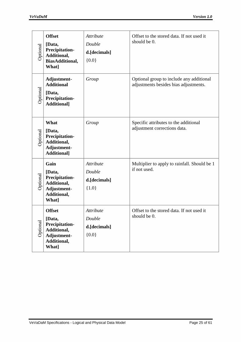
should be 0. O

pti

onal

Adjustment-

Additional

[Data,

Precipitation-

Additional]

Group Optional group to include any additional

adjustments besides bias adjustments.

Opti

onal

What

[Data,

Precipitation-

Additional,

Adjustment-

Additional]

Group Specific attributes to the additional

adjustment corrections data.

Opti

onal

Gain

[Data,

Precipitation-

Additional,

Adjustment-

Additional,

What]

Attribute

Double

d.[decimals]

{1.0}


if not used.

Opti

onal

Offset

[Data,

Precipitation-

Additional,

Adjustment-

Additional,

What]

Attribute

Double

d.[decimals]

{0.0}


should be 0.

VeVaDaM Version 1.0


5 Data specifications

All datasets are stored as dataset objects. Any of the types int, uint, float or double is

allowed (see section 3.1), and data compression using the associated Gain and Offset

attributes (see for instance Section 4.4) is possible. In general, it is highly recommended

to make use of int or uint to make the datasets as small in size as possible. As an example

the storage need for a single file and one year worth of data with 333x333 pixel values

are shown in Table 1. The numbers have been computed for three file types; one with

only the required data, one with all possible additional data and one with the required

data and interpolated data. The file sizes given are approximations since the actual file

size in a HDF5 file depends on values stored.Hence, on the amount of measured

precipitation.

Table 1: Example of storage space requirements for different types of VeVaDaM files using

unsigned integers and doubles respectively.

One timestep One year of data

File Temporal

Resolution

Uint8 Double Uint8 Double

Required 1 min ~ 0,12 Mb ~ 0,87 Mb ~ 66 Gb ~ 466 Gb

All additional data 1 min ~ 0,56 Mb ~ 4,28 Mb ~ 301 Gb ~ 2.305 Gb

Required incl.

interpolated data 10 min ~ 1,08 Mb ~ 8,48 Mb ~ 58 Gb ~ 456 Gb

The table clearly illustrates the advantages of not storing data in doubles since this may

take up as much as nine times more storage space. As data size is typically an issue in

the usage of real-time data, it is further recommended not to save redundant data, but

only the absolutely necessary. In all cases of choice it is preferred to save the precipitation

data (see Figure 2).

All the datasets are organized in groups which are shown in the following table in the

square brackets e.g. [Data/Precipitation].

Table 2: Required and optional datasets stored in VeVaDaM.

Name Type

Format

Description

Req

uir

ed

PrecipitationField

[Data/

Precipitation]

2D-array

Int,

uint,

Float or

Double

Actual precipitation field that can be

read directly or by using the attribute

“what” depending on the format.

VeVaDaM Version 1.0


Opti

onal

AdjustmentAdditional

[Data/

AdditionalAdjustement

]

2D-array

Int,

uint,

Float or

Double

Optional adjustment dataset that can

be read directly or by using the

attribute “what” depending on the

format.

Opti

onal

DistributedBiasAdditio

nal

[Data/

Bias]

2D-array

Int,

uint,

Float or

Double

Optional distributed bias factor

dataset that can be read directly or

by using the attribute “what”

depending on the format.

Opti

onal

PrecipitationFieldAddit

ional

[Data/

PrecipitationFieldAddit

ional]

2D-array

Int,

uint,

Float or

Double

Optional precipitation field dataset

that can be read directly or by using

the attribute “what” depending on

the format. Arrays are stored as one

long unpadded binary string starting

in the upper-left corner and

proceeding row by row (north to

south), from left (west) to right

(east).

Opti

onal

PrecipitationFieldInter

p_1…n

[Data/ Precipitation]

2D-array

Int,

uint,

Float or

Double

Interpolated additional precipitation

field matrices. The temporal

discretization implies the number of

matrices saved. The data can be read

directly or by using the attribute

“what” depending on the format.

Binary arrays are stored as one long

unpadded binary string starting in

the upper-left corner and proceeding

row by row (north to south), from

left (west) to right (east).

VeVaDaM Version 1.0


6 Standard and alternative processes

A number of methods and procedures have been developed and deployed over time to

achieve the best possible spatial and temporal precipitation signal from weather radar

measurements. The below list is not exhaustive or conclusive, but is at the time of writing

the procedures that best serve the purposes of most of the applications for the VeVa

partners.

For each of the processing steps the required documentation, along with the

recommended, optional, and alternative methods are stated below in Sections 6.1, 6.2,

and 6.3.

Overall it is recommended to adapt a standard set of processing steps that are suitable for

a given radar and location, and where only the parameters change over time.

The processing chain shown below is considered a standard and recommended

processing chain for VeVaDaM. The associated naming and reference to the attribute

holding the information is also given (see Section 4.2). Finally, the processing level for

these steps is given, meaning that application of any of these processes – with the

standards given here or alternative processes, means that the processing level should be

adjusted to the value given.

Table 3: Listing of the processes that are at the time of writing considered standard for the

VeVaDaM format, along with their naming, corresponding meta-data attributes and resulting

processing level.

Process Standard process

And reference

Meta-data and naming Process

ing

level

Clutter and

Noise reduction

Texture based

techniques.

[GABELLA]

\How\NoiceReduction

{GABELLA,

threshold =0.x, Gabella(2002)}

2

Attenuation

correction

Path Integrated

Attenuation.

[CapPIA]

\How\AttenuationCorr

{CapPIA,b=1.6, Harrison(2000)}

2

VPR correction Parameterized

bright-banding

VPRs

[BBVpr]

\How\VprCorr

{BBVpr, minDBz = 28, (J. a. Zhang

2010)}

2

Georeferencing,

gridding and

resampling

Nearest neighbor

[NearestNeighbor]

\How\Georef

{NearestNeighbor,

nneighbours = 3, none, (J. H. Zhang

2005)}

2

Z-R conversion Marshall-Palmer

conversion.

[MP]

\Data\ZRConversion

{MP, a:130;b:1.5, (Marshall 1948)}

2

VeVaDaM Version 1.0


Adjustment to

ground

observations

Mean field bias.

[MeanFieldBias]

\Data\Precipitation\What\BiasType

{MeanFieldBias, nneighbours = 3, (N.

&. Thorndahl 2014)}

3

Interpolation

between time

steps

Advection-based

blended.

[Nielsen]

\How\Interpolation

{Nielsen, step=1min, (Nielsen 2014) }

Not

applica

ble

Please do note that these steps are optional, but that they are recommended and that it is

required to document what methods have been used – even if the method is “none”.

6.1 Correction of raw data

The correction of raw data takes place prior to the data being stored in the VeVaDaM. It

is however a requirement that the processing carried out is documented in the VeVaDaM,

and therefore it is included here.

6.1.1 Clutter and Noise reduction

Purpose Clutter and noise reduction

Description This process removes artificial signals from reflective objects that are not

water. The correction can be achieved through dry weather signal

composition in various ways, or through using other radar parameters

besides reflectivity.

Required

Documentation

The clutter and noise reduction is considered to be part of the pre-

processing before data is stored in VeVaDaM. The requirement is therefore

to state the applied method or methods used in a way that makes it clear to

the user what quality of noise reduction has been carried out. I.e.

Method used

Any relevant parameters

Reference to further information on the method (some examples are

given below).

Considerations

and background.

Noise and clutter depends to a high degree on the location and the type of

radar – and not-least the internal radar processing (which occurs in many

cases). VeVa encourages that the physics of the rainfall is used in the noise

reduction. Also, although peak rainfall intensities are interesting and

important – it is more important to capture the correct total mass.

It is recommended, but not required, that the noise reduction is carried out

in polar coordinates.

VeVaDaM Version 1.0


Recommended

methods

Texture-based techniques. From the existing literature and applications,

it is believed that using the neighboring cells in both space and time is the

best approach since it can be carried out in real-time. This includes using

“dry weather” filters – but care should be taken when dry weather signals

cannot be attributed to known effects and sources. Such as Gabella et.al.

(2002)

Part A: Large reflectivity gradients.

Part B: Comparing area to circumference of contiguous echo

region.

Alternative

methods Beam-blockage using DEM should be performed prior to other

filters, and should not be done alone. It may be compensated using

spatial interpolation methods.

Fuzzy-logic based on polarimetric moments.

Filtering based on cloud type. Since cloud type is not generally well

established, and typically mixed during events.

Histogram based clutter identification based on occurrences or

historic thresholds. This typically requires very consistent datasets

with long periods and is not recommended.

Base cut-off – thresholds. Although a minimum threshold can make

sense in some cases, it must be argued why that threshold exist. The

concern is that removes total rainfall and early detection.

References (Gabella 2002) and (Ośródka 2014)

VeVaDaM Version 1.0


6.1.2 Attenuation correction

Purpose Damping corrections

Description The radar beam loses energy in a number of different ways that is not

associated with the precipitation in the actual bin. Damping due to the

distance travelled, general meteorological conditions and not least the

accumulated precipitation between the radar and the bin in question

affects the intensity as seen by the radar.

Ideally independent measurements from other radars or other

wavelengths may be used, but the method recommended below has

proven to be both efficient and stable.

Required

Documentation

The damping corrections reduction is considered to be part of the pre-

processing before data is stored in VeVaDaM. The requirement is

therefore to state the applied method or methods used in a way that

makes it clear to the user what artifacts may have been introduced or

assumed removed through stating:

The method used


References to further information on the method (some examples

are given below).

Considerations

and background.

Damping corrections is best done on the individual beam burst in

combination with meteorological information measured, modelled or

seasonal. Typically, the damping correction is carried out by integrating

intensities and effects from the bins nearest the radar and progressively

out to the limit of the radar signal.

It is recommended, but not required, that the damping correction is

carried out on individual elevations and bursts in polar coordinates.

Recommended

methods

Path Integrated Attenuation calculations are recommended, in particular

ones that may be applied in real-time and are stable also in relation to

clutter effects.

Kraemer and Verworn developed and tested an iterative method of the

above which is recommended.

Alternative

methods

Cap PIA (Path Integrated Attenuation) (Harrison 2000)

Reference (Krämer 2008)

VeVaDaM Version 1.0


6.1.3 Vertical Profile of Reflectivity (VPR) correction

Purpose VPR correction

Description The VeVaDaM stores surface precipitation, and therefore the 3-

dimensional radar signals must be transformed to a surface precipitation

while taking into account the variations in reflectivity due to differences

in air density, bright banding and other effects due to the meteorological

stratification, measured or assumed as a vertical profile of reflectivity.

Required

Documentation

The VPR correction must be carried out before data is stored in

VeVaDaM. The requirement is therefore to state the applied method or

methods used in a way that makes it clear to the user what quality of

correction has been carried out. I.e.

Method used


Reference to further information on the method

Considerations

and background

The vertical distribution of precipitation (and thus reflectivity) is

typically non-uniform. As the height of the radar beam increases with

the distance from the radar location (beam elevation, earth curvature),

one radar burst samples from different heights even if emitted

horizontally. The effects of the non-uniform VPR and the different

sampling heights need to be accounted for as we are interested in the

precipitation near the ground or in defined heights. VPR corrections

includes the compensating for bright-banding.

Recommended

methods

VPR corrections may be done prior to or during the 2D interpolation.

Reference (J. a. Zhang 2010)

VeVaDaM Version 1.0


6.1.4 Georeferencing, gridding and resampling

Purpose From polar scans to a regular geo-referenced grid.

Description As the radars are generally rotating at a certain speed and emitting beams

with another frequency, two full-rotations are not generally emitting

beams at all the same angles. The data has to be gridded and

georeferenced for further processing.

Required

Documentation

The various coordinate transformations required to arrive at a rectangular

2D surface precipitation field cannot be reversed, and consequently any

alternative methods must be implemented from the raw radar signals.

The intention in VeVaDaM is to give a general description of the methods

used, so that the end user can infer any consequences for the downstream

use of that data.

Do note that VeVaDaM requires the precipitation field to be gridded

with one of the resolutions in the DKN grid.

Considerations

and background.

The majority of the pre-processing described in this section (clutter,

blockage, attenuation, damping, etc.) is best done on the raw beam radar

data. It is not practical to describe all processing, as some also is going on

within the radar factory software, but please do keep the user in mind

when documenting this.

Recommended

methods

The variability and applicability of different methods depend to a high

extent on radar type and location. The recommended methods are

therefore very generically described as Nearest neighbor or spline

interpolation.

Alternative

methods

Any applicable methods.

Reference (J. H. Zhang 2005)

VeVaDaM Version 1.0


6.2 Conversion to surface precipitation

6.2.1 Z-R from reflectivity to precipitation

Purpose Z-R conversion

Description The reflected energy from the radar burst, after noise reduction and

various corrections, is a result of the amount of water droplets in the

atmosphere. Hence the reflectivity measurements have to be converted to

precipitation rates before applied for hydrological purposes.

Required

Documentation

The Z-R conversion is considered to be a reversible process in VeVaDaM,

although it is typically non-linear. The idea is that sufficient information

should be included to derive the (corrected) reflectivity, and therefore Z-

R conversion has its own group in the metadata, where the user is required

to document.

Method used

Parameter a

Parameter b

Optional Parameter c

Considerations

and background.

From the first correlations of reflectivity to drop sizes made on dyed filter

papers to the present disdrometer correlations the relationship between

reflectivity and precipitation rate has remained remarkably robust.

Recommended

methods

Marshall-Palmer – two parameter power law function Z = a x Rb. This is

recommended since VeVaDaM allows for a spatial adjustment to rain

gauges where spatial variability may be incorporated.

Alternative

methods

Droplet size based corrections if droplet size distributions are available.

Reference (Marshall 1948)

VeVaDaM Version 1.0


6.2.2 Adjustment to ground observations

Purpose Using in-situ ground observations for adjustment of weather radar

rainfall

Description Rain gauges often provide accurate and reliable point measurements of

rainfall. The spatial rainfall estimate provided by the radar may be

adjusted to ground observations to reflect these measurement.

Traditionally, multiple rain gauges have been used for the adjustment.

Other ground observations, such as disdrometers and runoff

measurements can also be used.

Required

Documentation

Adjustment to ground observations is central to VeVaDaM and updating

the adjustments is expected to be one of the main uses of the data model,

from a simple real-time adjustment, over an improved adjustment using

several time steps, hours and days. It is also expected that bias adjustments

will be both mean field (scalar) and distributed (matrices). It is further

expected that the adjustment to rain gauges is fully reversible by the end

user of VeVaDaM.

The required documentation of what has been applied is therefore central

and includes:

Method used


Ground observations used (e.g. stations used)


Considerations

and background.

The aim of VeVaDaM is to achieve the best possible spatial precipitation

field. Radar and rain gauges have each their strengths and weaknesses,

and it is therefore expected that the combination of the two can provide

the best of both worlds. In practice the best method to use depends on

several factors ranging from type of precipitation, terrain, time of year,

age of measurement, number and type of rain gauges etc.

Recommended

methods

Mean field bias (daily, hourly, etc.)

Nearest neighbor adjustments.

Inverse distance weighting.

Kriging.

Alternative

methods

Event based adjustments – given a clear definition of how events are

determined and characterized.

Reference (N. &. Thorndahl 2014)

VeVaDaM Version 1.0


6.3 Data interpolation

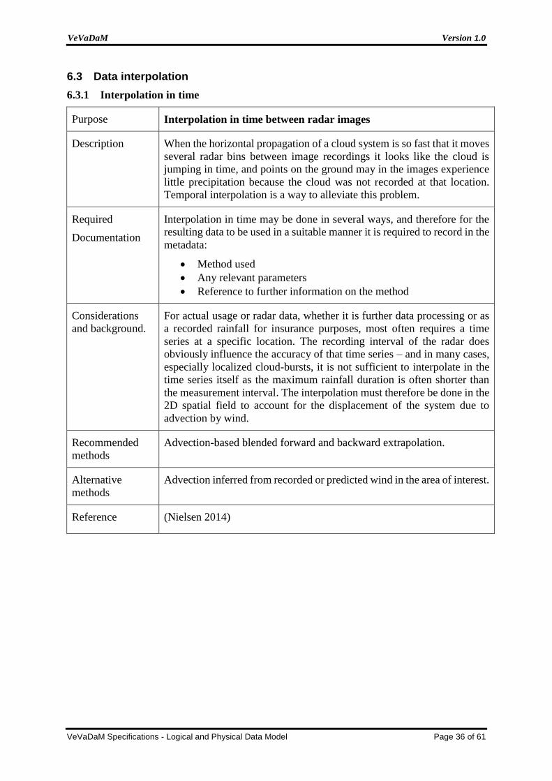
6.3.1 Interpolation in time

Purpose Interpolation in time between radar images

Description When the horizontal propagation of a cloud system is so fast that it moves

several radar bins between image recordings it looks like the cloud is

jumping in time, and points on the ground may in the images experience

little precipitation because the cloud was not recorded at that location.

Temporal interpolation is a way to alleviate this problem.

Required

Documentation

Interpolation in time may be done in several ways, and therefore for the

resulting data to be used in a suitable manner it is required to record in the

metadata:

Method used



Considerations

and background.

For actual usage or radar data, whether it is further data processing or as

a recorded rainfall for insurance purposes, most often requires a time

series at a specific location. The recording interval of the radar does

obviously influence the accuracy of that time series – and in many cases,

especially localized cloud-bursts, it is not sufficient to interpolate in the

time series itself as the maximum rainfall duration is often shorter than

the measurement interval. The interpolation must therefore be done in the

2D spatial field to account for the displacement of the system due to

advection by wind.

Recommended

methods

Advection-based blended forward and backward extrapolation.

Alternative

methods

Advection inferred from recorded or predicted wind in the area of interest.

Reference (Nielsen 2014)

VeVaDaM Version 1.0


7 Physical data model specifications

The physical data model implementations of the logical data model VeVaDaM described

in the preceding sections most follow those specifications. In addition, for the approved

physical data models there are some additional requirements that are described below.

At the time of writing the only physical data model supported is the VeVaDaM_H5, i.e.

a file based format based on HDF5.

This format is chosen for its multiplatform usage, its adaptation by the ODIM group, and

in general a wide support by a global usergroup and accessible through libraries that are

supported in multiple programming languages.

7.1 Additional specifications for file based data models

As specified in section 4.1 the data model is designed to contain only one time step. For

physical data models this imposes additional requirements to increase the usability and

management of the potentially large datasets.

7.1.1 File naming specifications

The VeVaDIM H5 files, has to be named in a specific way. The name is comprised of:

- 4 characters long identification, which are unique for the specific radar.

- DateTime formatted as YYYYMMDDHHmmss (year: YYYY, month: MM, day:

DD, hour: HH, minute: mm and second: ss).

…\[Char(4)][ YYYYMMDDHHmmss].h5

An example hereof is:

…\StRe20161105010900.h5

7.1.2 Folder structure specifications

The folder structure of the physical data model implementation follows a date based

structure of year, month and day. The structure comprises of:

- Year formatted as YYYY

- Month formatted as MM

- Day formatted as DD

…\YYYY\MM\DD\

An example hereof is:

…\2016\11\05\StRe20161105010900.h5

The advantage of the physical data model is its simplicity.

VeVaDaM Version 1.0


8 Tools for editing and using VeVaDaM

The VeVaDaM physical data model implementation as a HDF5 file, ensures that there

are a number of tools readily available for creating and using these files. It is fully

encouraged to build additional tools that supports VeVaDaM just as the VeVa

collaboration encourages that existing software is extended to read and write the

VeVaDaM format.

The present version 1.0 of the VeVaDaM and the associated example files have been

tested in the following software.

Table 4: Software packages that have been tested with VeVaDaM example files.

Software

package

About and usage Versions

tested

MATLAB MATLAB is a general toolbox for working with data,

including analysis and presentation.

2016b for

windows

HDFView This package is maintained by HDF group with regular

updates. It is possible to both view and edit files.

v.2.11 for

windows

.Net library :

HDF5DotNet

This programming package is no longer being supported,

but works well for simple usage of HDF5 and is more high

level than the HDF.PInvoke. Both libraries are available

via NuGet.

v.1.8.9

using .net:4.6.1

Python

package:

h5py

This package is actively updated by the community and is

available via “pip install h5py” on most platforms [on

windows Anaconda or Miniconda are recommended]

v.2.6.0 from

anaconda

running

Python 3.5.2.

VeVaDaM Version 1.0


9 References

Danmarks statistik og Kort & Matrikelstyrelsen. Det Danske Kvardratnet v.2. - Faktaark.

København: Danmarks statistik, 2012.

Gabella, M. and Notarpietro, R. “Ground clutter characterization and elimination in mountainous

terrain. In Use of radar observations in hydrological and NWP models.” Katlenburg-Lindau,

Copernicus, URL: http://www.copernicus.org/erad/online/erad-305.pdf, 2002: 305–311.

Harrison, D.L., Driscoll, S.J. and Kitchen M. “Improving precipitation esitmates from weather

radar using quality control and correction techniques.” Meteorological Applications , 2000:

6, 135 - 144.

HDF-Group. Hdf5group.org. 4 December 2016. https://www.hdfgroup.org/hdf5/.

Krämer, S., Verworn, H.-R. “Improved C-band radar data processing for real time control of

urban drainage systems.” 11th International Conference on Urban Drainage, Edinburgh,

Scotland, UK, 2008, 2008: 1-10.

Marshall, J.S. and Palmer, W.M. “The distribution of raindrops with size.” Journal of

meteorology, 1948: Vol 5, 165-166.

Michelson, Lewandowski, Szewczykowski and Beekhuis. EUMETNET OPERA weather radar

information model for implementation with the HDF5 file format. EUMETNET OPERA,

2014.

Michelson, Lewandowski, Szewczykowski and Beekhuis. EUMETNET OPERA weather radar

information model for implementation with the HDF5 file format, version 2.2. Document,

Eumetnet OPERA, 2014.

Nielsen, J.E., Thorndahl, S.L. and Rasmussen, M.R. “A numerical method to generate high

temporal resolution precipitation time series by combining weather radar measurements with

a nowcast model.” Atmospheric Research, 2014: 1-12.

Ośródka, K., Szturc, J. & Jurczyk, A. “Chain of data quality algorithms for 3-D single-

polarization radar reflectivity (RADVOL-QC system).” Meteorological Applications, vol. 21,

no. 2, 2014: 256-270.

Thorndahl, et.al. “Weather radar rainfall data in urban hydrology.” Hydrology and Earth System

Sciences, 7 March 2017: 1359-1380.

Thorndahl, Nielsen & Rasmussen. “Bias adjustment and advection interpolation of long-term

high resolution radar rainfall series.” Journal of Hydrology, 2014: 214-226.

Zhang, J. and Qi, Y. “A Real-Time Algorithm for the Correction of Brightband Effects in Radar-

Derived QPE.” Journal of hydrometeorology, 2010: Vol 11, 1157 - 1171.

Zhang, J., Howard, K., Gourley, J.J. “Constructing three-dimensional multipleradar reflectivity

mosaics: examples of convective storms and stratiform rain echoes.” Journal of Atmospheric

and Oceanic Technology 22 (1), 2005: 30-42.

VeVaDaM Version 1.0


APPENDIX A - An Introduction to Weather Radars

Accurate estimates of the spatial and temporal distribution of precipitation

(spatiotemporal distribution) is essential for determining the correlation between

precipitation and runoff. Precise precipitation estimates can improve design and control

of stormwater drainage systems and wastewater treatment plants (WWTP) during heavy

rainfall. An optimized integrated real time control of stormwater drainage system and

WWTP makes it possible to utilise system capacity efficiently. Hence, it is possible to

reduce damage cost due to precipitation related flooding and reduce combined sewer

overflows to minimize the environmental impact on recipients and ensure bathing water

quality. Furthermore, accurate precipitation estimates is vital for detailed retrospective

analyses of how a given stormwater system reacted to a given precipitation event.

By the use of weather radars, it is possible to obtain good estimates of the precipitations

spatiotemporal distribution over a larger area. At the time of writing, it is not feasible to

obtain precipitation estimates with similar spatiotemporal resolution with other

technologies. By the use of weather radars, it is possible to measure the precipitation

variability three-dimensionally in the lower part of the atmosphere. The basic

measurement principle of all weather radars are the same, but the size of the measurement

area, accuracy and spatiotemporal resolution is depended on the given weather radar

type.

A weather radar measures precipitation by emitting an electromagnetic pulse into the

atmosphere in a given direction and elevation. When the electromagnetic pulse hits

something in the atmosphere, a part of the emitted energy is reflected back towards the

radar. The radar in turn detects the reflected energy. The basic measurement principle is

illustrated in Figure 3.

Figure 3: Illustration of how an emitted electromagnetic pulse from a weather radar is reflected

by water droplets in a precipitation system in the atmosphere (Ahm, 2017).

Weather radars can be categorised by the electromagnetic wavelength they utilise. The

most common frequency-bands utilised for land-based civil weather radars are S-band,

C-band and X-band.

S-band radars uses wavelengths between 7.50-15 cm and a frequency of 2-4 Ghz.

C-band radars uses wavelengths between 3.75-7.50 cm and a frequency of 4-8 Ghz.

X-band radars uses wavelengths between 2.50-3.75 cm and a frequency of 8-12 Ghz.

These three types of weather radars have different advantages. Longer wavelengths will

result in less attenuation of the signal. By using S and C-band weather radars it is possible

obtain measurement ranges up to 250 km. The disadvantages of S and C-band weather

radars are that large antennas are required, which result in high hardware, installation and

VeVaDaM Version 1.0


maintenance costs. The combination of the radars large physical dimensions and long

measurement range result in slow rotation speed compared to smaller X-band weather

radars. Therefore, it is often not possible to obtained the desired spatiotemporal

precipitation resolution for urban drainage applications of 1-5 min and 1km2 (Schilling,

1991; Berne et al., 2004; Einfalt et al., 2004; Thordahl et al, 2017. By the use of X-band

weather radars it is possible to obtain the desired resolution. Some X-band weather radars

offer a resolution of <1 min and <0,05km2.

The disadvantages of X-band weather radars are the increased attenuation of the signal

compared to C and S-band weather radars. This result in measurements ranges <50 km

for must X-band weather radars. The increased attenuation is due to the increased

measurement sensitivity of X-band weather radars, which allow for detection of smaller

water droplets than C and S-band weather radars. The increased sensitivity is also an

advantage for urban drainage applications since the measurement accuracy of low

intensity precipitation is increased. Due to the smaller physical size of X-band weather

radars it is often easier to place them optimal in relation to the desired measurement area

(hydrological catchment). Furthermore, hardware, installation and maintenance costs are

significant lower for X-band weather radars compared to C and S-band weather radars.

A major challenge of precipitation measurement with a weather radar is that a weather

radar, in principle, cannot distinguish precipitation and other objects in the atmosphere.

Figure 4 illustrates some of the most common phenomenons.

Figure 4: Illustration of different atmospheric sources which can affect the precipitation

measured by weather radars (Ahm, 2017).

Figure 4 illustrates some of the most common phenomenon’s that can affect the

precipitation measurement with weather radars. Hence, it is important to consider these

effects when installing and using a weather radar. Some of the effects illustrated in Figure

4 can be minimized by placing the weather radar optimal in relation to the catchment of

interest. The application of weather radar for precipitation measurement is described

further in the book Radar for Meteorologists (Rinehart, 2010). Multiple research projects

have been conducted within the field of weather radar applications for urban hydrology.

For example Vejrradarbaseret styring af spildevandsanlæg I (Rasmussen et al., 2008),

Vejrradarbaseret styring af spildevandsanlæg II (Thorndahl et al., 2010), Combining C-

and X-band Weather Radars for Improving Precipitation Estimates over Urban Areas

(Nielsen, 2013), Combining weather radar nowcasts and numerical weather prediction

models to estimate short-term quantitative precipitation and uncertainty (Jensen, 2015)

and Adjustment of rainfall estimates from weather radars using in-situ stormwater

drainge sensors (Ahm, 2017).

VeVaDaM Version 1.0


The Danish Meteorological Institute (DMI) operates five C-band weather radars, which

in combination covers must of Denmark. The location and coverage is illustrated in

Figure 5 together with the location of the 157 active SVK rain gauges (august 2015).

Figure 5: Map over Denmark which show the location of DMI’s five C-band weather radars and

the 157 active SVK rain gauges (august 2015) (Ahm, 2017).

The spatiotemporal resolution of DMI’s standard weather radar product is 2000x2000m

every 10 minutes. However, a spatiotemporal resolution of 500x500 every 5 minutes can

be provided by DMI. The Furuno WR-2100 X-band weather radar utilises a shorter

wavelength than DMI’s C-band weather radars. Hence, the advantages of the WR-2100

is a better spatiotemporal resolution and a significant smaller physical size. The

disadvantages of the WR-2100 is the significant shorter measurement range (30-50 km)

compared to DMI’s C-band weather radars.

Beside the direct usages of weather radar data for water utility companies, weather radar

data can result in other benefits for society, municipalities and citizens. Weather radar

data can be used for hydrological modelling of the whole water cycle and warning

systems of potential flooding, poor road conditions or just notifications of when it is

smart to take in laundry or bike home from work.

VeVaDaM Version 1.0


References

Ahm, M. (2017) Ph.D. Thesis: Adjustment of rainfall estimates from weather radars using in-

situ stormwater drainge sensors, Department of Civil Engineering, Aalborg University.

Berne, A., Delrieu, G., Creutin, J.-D., Obled, C. (2004) Temporal and spatial resolution of rainfall

measurements required for urban hydrology. Journal of Hydrology, 299(3–4), 166–179. DOI:

http://dx.doi.org/10.1016/j.jhydrol.2004.08.002.

Einfalt, T., Arnbjerg-Nielsen, K., Golz, C., Jensen, N.-E., Quirmbach, M., Vaes, G., Vieux, B.

(2004) Towards a roadmap for use of radar rainfall data in urban drainage. Journal of

Hydrology, 299(3–4), 186–202. DOI: http://dx.doi.org/10.1016/j.jhydrol.2004.08.004.

Jensen, D. G. (2015) Ph.D. Thesis: Combining weather radar nowcasts and numerical weather

prediction models to estimate short-term quantitative precipitation and uncertainty,

Department of Civil Engineering, Aalborg University.

Nielsen, J. E. (2013) Ph.D. Thesis: Combining C- and X-band weather radars for improving

precipitation estimates over urban areas, Department of Civil Engineering, Aalborg

University.

Rasmussen, M. R., Thorndahl, S., Grum, M., Neve, S., Borup, M. (2008) Vejrradarbaseret

styring af spildevandsanlæg, København.

Rinehart, R. E. (2010) Radar for Meteorologists, Rinehart Publications.

Schilling, W. (1991) Rainfall data for urban hydrology: what do we need? Atmospheric Research,

27(1–3), 5–21. DOI: http://dx.doi.org/10.1016/0169-8095(91)90003-F.

Thorndahl, S., Rasmussen, M. R., Neve, S., Poulsen, T. S., Grum, M. (2010) Vejrradarbaseret

styring af spildevandsanlæg II. DCE Technical Report, 95(95), Aalborg University, Denmark.

Thorndahl, S., Eifalt, T., Willems, P., Nielsen, J.E., Veldhuis, M.t., Arnbjerg-Nielsen, K.,

Rasmussen, M.R., and Molnar, P. (2017) Weather radar rainfall data in urban hydrology.

Hydrology and Earth System Sciences, 21, 1359-1380. DOI: http://dx.doi.org/10.5194/hess-21-

1359-2017

VeVaDaM Version 1.0


APPENDIX B - Envisioned uses of Weather Radar Data

Uses of radar data varies across the Danish water sector today. The table below summarises the present and envisioned uses of radar data based on a

discussion between the VeVa partners. The envisioned usage has been a point of reference in designing the logical structure of the data model and

the associated metadata and is therefore included for reference.

Decision objectives Application of radar data Usage today and future relevance

Pla

nn

ing

General long term planning

(>10 years)

(E.g. Dimensioning of new waste

water treatment plants and storage

basins)

The long term planning is predominantly influenced by

other parameters than the spatial distribution of

precipitation, however it may play a role in defining for

instance utility KPIs. In the extended term including

climate change considerations it is more likely the

change in spatial precipitation patterns that will

influences the long term planning.

Not relevant today due to the short

duration of measured time series. Over

prolonged periods of radar data recorded,

the spatial distribution is likely to

supplement the analysis.

Medium term planning

(5-10 years)

(E.g. Sewer renovation plans)

In the medium-term planning the local topography and

open water areas can in some areas have large effects,

and it can therefore be relevant to include spatial

precipitation in the overall planning.

Not in use today. With longer high

resolution radar time-series and further

developments of processing tools the

applicability is likely to increase.

Detailed short term planning

(1-5 years)

(E.g. Local area renovation

projects)

Distributed precipitation can potentially be applied for

mass-balance computations for smaller catchments and

hereby give valuable input for monitoring the

performance of sewage systems and locate intruding

and unwanted water. For the analysis and dimensioning

of sewage systems the distributed precipitation can

potentially provide a more accurate input taking the

local spatial variations into account.

Cautious initial applications today. A

track-record and as above improved

processing technologies and tools will

likely increase the usage.

VeVaDaM Version 1.0



Supporting models and analysis

tools

(E.g. Model input and validation)

Distributed precipitation can be applied as more precise

inputs for hydrological modelling and hereby reduce the

uncertainty. Furthermore, the data are applicable for

validation due to the high spatial and temporal

resolution of radar data.

Only applied for a limited number of

applications due to a lack of

consistency/quality in the measurements

and processing. It is to be expected that

radar data will become more commonly

applied in the foreseeable future.

Dail

y o

per

ati

on

s

Daily operation and

background information

(E.g. Gauge diagnostics)

Distributed data may be applied during or shortly after

events to control hydrological systems in real time, such

as distributing the flows in urban drainage systems

through basins and pumping stations. Furthermore, the

data may be used to monitor and pinpoint faulty gauges

and specifically compute overflows.

Some utilities apply the data today and

more expect to use it in the near future due

to the increases in data availability and

quality.

Service and maintenance

(E.g. Probability for dry weather

with hours lead time)

Radar data can potentially be used to produce dry

weather forecasts, which through a hydrological

forecasting system can be used to inform maintenance

which area to safely operate in. Using radar in the

context can likely improve forecast reliability and hence

enable optimization on plant operations.

Meteorological institutes offer publicly

available radar images that are used today.

The expectation is that more specialized

products within a short number of years

will extend the usage.

Real time control of waste water

treatment plants

(E.g. Switching treatment mode

between dry and wet weather

operation)

Depending on the specific catchment the distributed

precipitation information can give a warning to the

waste water treatment plant with a lead time

corresponding to the run-off - and concentration time.

Real time control and hydrometeor classification has a

high potential in relation to real time operation and

discharge strategy for the waste water treatment plants.

Is actively applied today. With increasing

data consistency/quality it is the

expectation and potential for further

implementation also for smaller

catchments.

VeVaDaM Version 1.0



Warn

ing

Hydrological forecasting,

bathing water

(E.g. Probability for combined

sewer overflows)

The distributed precipitation can be used to model and

predict overflows along with risk management and

warnings for stakeholders. A warning system can be

used to close public bathing areas before contamination

of the bathing waters from CSOs.

Is today being tested in a few utilities, but

is expected to be more commonly

implemented in the coming years.

Hydrological forecasting,

flooding

(E.g. Area specific warnings)

Hydrological forecasting using distributed precipitation

as input can potentially be used to predict and estimate

flooding of urban areas.

The application is currently being tested.

The actual responsibility in Denmark lies

with the emergency authorities and

municipalities.

Soci

ety

Customer service

(E.g. Information about area

specific return periods for rainfall)

Distributed precipitation data may be of interest to the

public, as general information and for more specific

purposes such as documentation of cloud burst in an

insurance context.

In use today in several utilities. One utility

has implemented a publicly available

online application for documenting cloud

bursts.

VeVaDaM Version 1.0


APPENDIX C - Dictionary of VeVa terminology

Name

[Danish equivalent]

VeVa definition

[Reference for further info where relevant]

Adjustment of data.

Bias adjustment.

[Justering]

The process of adjusting the interpreted precipitation to ground

observations, typically from raingauges.

Attenuation

[Attenuering]

The gradual loss of intensity in the radar reflection as it passes

through the atmosphere. The amount of attenuation is a function

of the amount of droplets reflecting the radar, the distance from

the radar, but it can also be affected by other factors.

Azimuthal resolution/

/beam separation

[Azimut opløsning]

Is a measure of the angular-distance between two radar beams,

and thus also a measure of the total number of beams that are

transmitted as the radar rotates a full circle. Typical examples are

0.5° for specialized radars and more typically 1°.

Beam-blockage Nearby high objects or topography may block entire beams of the

radar – ie. certain subsections.

Beamwidth

[Stråle bredde]

A single radar beam in meteorological applications is made as

narrow as possible both horizontally and vertically, but it is a

transmitted as a cone rather than a line. The width of the cone is

measured in degrees and is a result of the radar architecture, but

can in some instances be varied. Typical examples are between

1,0° and 3,0°.

Bright banding

Effect of frozen water particles in the atmosphere which due to

their more reflective surface has a higher relative reflectivity.

Calibration of radar

[Kalibrering]

The process of radar calibration is the tuning of the radar

hardware and the electronic components.

CAPPI (Pseudo Cappi)

Constant Altitude PPI [plan position indicator] is a derived

product where rather than providing reflections in elevations the

reflections are given in a constant height above ground. Pseudo

CAPPI combines different heights to obtain a homogenous

surface product.

Correction of reflectivity

[Korrektion]

The process of correcting the reflectivity measured by the radar

for atmospheric, topographic and other physical conditions that

affects the signals. This includes attenuation, ground clutter,

VPR, etc.

dBZ - decibels

[dBZ]

A measurement unit used for measuring the energy in a wave,

typically the amplitude of the wave. This is a logarithmic unit

(dimensionless).

VeVaDaM Version 1.0


Elevations

[Elevationer]

The angle relative to horizontal at which the radar beam is

admitted. Ideally the elevation closest to horizontal [0°] is the best

measure of the rainfall at the surface, but it is also the elevation

most polluted by ground clutter and other non-rain related echoes.

Ground clutter

[Overflade echoer]

Non-precipitation signals due to the radar beam being diverted or

reflected by objects on or near the ground. Examples are tall

building, bridges, wind farms, or even dust or pollution in the

lower atmosphere. Ground clutter will not move in time, but small

differences in the signal will still be seen due to atmospheric

conditions changing over minutes and with seasons. Therefore

ground clutter is not constant and some care must be taken to

adjust for ground clutter. Sidelobe effects are also typically

grouped with ground clutter.

HDF5 Hierachical Data Format – version 5. Data format for storing and

organizing large amounts of data.

[https://support.hdfgroup.org/HDF5/]

OPERA

European Operational Program for Exchange of Weather RAdar

Information.

European collaboration for operationally-oriented weather radar

issues, including development, distribution and generation of

high-quality pan-european radar data.

[http://www.eumetnet.eu/opera]

Pixels/Bins/Gates

[Pixler – opløsning]

The unit spatial area where the radar reflectivity is determined.

This is a ring-segment with a height equal to the radial resolution

[in meters] and a width in the azimuthal resolution [in degrees].

PPI Plan position indicator is a type of radar display with the radar in

the center and a continuous update of the plot with the sweeping

beam, drawn one elevation on top of the last.

Radial resolution

[Radial opløsning]

The number of bins for a given distance that the beam travels

away from the radar. This is closely linked to the frequency and

shape of the radar pulse and varies with types of radar. Examples

ranges from 50m for a high resolution X-band radar to 2 km for a

low resolution C-band radar.

Radials

[Radialer]

The center lines of the radar beams as they are emitted from the

radar. The distance between two adjacent radials is the azimuthal

resolution.

Reflectivity

(Base reflectivity)

[Reflektivititet]

The relative amount of power returned to the radar compared to

the transmitted power. It is a function of the atmosphere, the

system and other reflective surfaces and particles in the

surroundings. Unit of reflectivity (Z) is mm6/m3.

VeVaDaM Version 1.0


Sea clutter

[Bølge echoer]

Effects of reflections of the water surface – typically from waves.

Sidelobes

[Sidereflektans]

Unlike laser beams, radar beams are not perfectly straight beams,

but rather imperfect cones of energy. The implication is that some

of the energy transmitted will be received at other frequencies and

from other directions than the intended. These effects appear as

contamination along with ground clutter.

Sub and Super-refraction

Anomalous propagation

[Refraktion]

Bending of the radar beam due to changes in the density of the air

through which it travels. Often this is simplified into a vertical

description of the variability (ie. constant over the area) as a VPR.

Sun flares

External emitters

[Falske echoer]

Signals received from transmitters sending on or near the same

frequencies as the radar signal. Can be other radars, certain

wireless networks. Named as sun flares because they appear on

the map as a sun beam.

Vertical Profile of

Reflectivity (VPR)

[VPR]

Precipitation is 3-dimensional in space. The vertical distribution

of precipitation (and thus reflectivity) is typically non-uniform.

As the height of the radar beam increases with the distance from

the radar location (beam elevation, earth curvature), one sweep

samples from different heights. The effects of the non-uniform

VPR and the different sampling heights need to be accounted for

to accurately estimate the precipitation near the ground or at a

defined height.

VeVaDaM Version 1.0


APPENDIX D - Walkthrough of VeVaDaM examples

Physical File format examples

As described in the specifications the physical implementation of VeVaDaM is flexible

with several meaningful combinations. This appendix provides a walkthrough of the

three example files that are attached to the documentation as examples.

These three examples are not intended to be used as templates, nor intended to express

the full range of how the data model may be used. Instead they are intended to illustrate

how the format may be used, and provide an illustration of what the physical data model

may contain.

The three example files are:

VeVa20160214235959_Required.h5

VeVa20160214235959_Additional.h5

VeVa20160214235959_Interpolated.h5

In the following sections, screen shots from the HDFView tool provided by the HDF-

Group in version 2.11 are shown. This tool is freely available for Windows, Mac and

Linux from the HDFgroup website at:

https://support.hdfgroup.org/products/java/hdfview/

Minimum required file structure

Walkthrough of the file: VeVa20160214235959_Required.h5

This file is a typical example of a VeVaDaM file being created in real-time, with minimal

processing and mean field bias adjustment factor of 1.0 – ie. no adjustement made.

Figure 6 below illustrates the most basic structure of a VeVaDaM file. It contains only

the minimum required meta-data given as attributes and one precipitation dataset, the

dataset “PrecipitationField”.

Figure 6: Schematization of VeVaDaM H5 file physical implementation of the data model with

only the minimum required data.

The hierarchical structure of the file is read from left to right, starting from the root level

to level 2 in the above example. The file contains groups, a dataset and attributes, as

defined in the documentation. Each of these groups of attributes are discussed below.

https://support.hdfgroup.org/products/java/hdfview/

VeVaDaM Version 1.0


Opening the file in any tool capable of reading HDF5 files will reveal the structure and

allow the user to read the attributes and the dataset. Figure 7 is a screenshot from

HDFview after opening the file, expanding all the groups and selecting the dataset.

Figure 7: Example of a VeVaDaM H5 file containing the required data displayed with the

program HDF-view. Box number 1 displays the hierarchical structure of the file. Box number 2

shows the attributes associated with the selected dataset or folder selected/highlighted in box 1.

Box number 3 shows the dataset selected in box number 1.

On the left in the first box is shown the same structure as shown in Figure 6, where the

group level is shown by the indentation level and the tree structure. When a group or a

data set is selected the associated attributes are shown at the bottom in the second box.

Finally the right hand box number three is used for displaying datasets either as an image

as in this example or in a tabular form.

On the root level the three attribute groups How, What and Where stores metadata

associated with all data in the file, ie. How the data was recorded and how it has been

processed, What data is contained in the file, i.e. time and date of the recording, and

Where geographically the radar was located, including the coverage through the Range

attribute, in this case 50 kilometers and 50 centimeters. The three attribute groups are

shown with all their associated attributes in Figure 8.

VeVaDaM Version 1.0


Figure 8: The three required root groups and their associated attributes as shown in HDFview.

The next level of metadata is located in the Data group, and is therefore associated

specifically with the data contained in that group. The three metadata groups are What,

Where and ZRConversion, and they are shown below along with their attributes. For the

Data group the Where group gives the dimension of the 2-dimensional dataset, along

with the timestamp (date and time) of the precipitation dataset.

The Where group contains the vertical reference for the 2-dimensional dataset (in this

case 1000m above ground), the resolution of the grid (in this case 250m x 250m) and

finally the DKN cell of the lower left corner of the grid. Do note in this case that the

100m DKN is used for the anchor of the grid although the cell size is 250m – this is

perfectly fine.

Finally the ZRConversion group details how the conversion from reflectivity to

precipitation has been done. I this case a standard Marshall-Palmer conversion has been

used with the a and b parameters given (see Section 6.2.1).

VeVaDaM Version 1.0


Figure 9: Meta-data attributes associated with the first level Data group, associated with all the

datasets in the substructure.

The second level of attributes are associated with the Precipitation dataset specifically,

and since the Where, When and How are all been inherited from the parent levels, the

remaining information is a What group associated with how the data values are stored.

Figure 10 shows the attributes of the Precipitation group in the root and in the What sub-

group respectively. All attributes are associated with the PrecipitationField and is in this

case shown together with the tabular values of a section of the dataset. The

Precipitation/root attribute “BiasRealTimeMeanField” signifies what value has been

used to adjust the precipitation field to ground observations. In this case the value of 1.0

signifies that the values have not been altered, either because no adjustment was made or

the precipitation measured by the radar was un-biased.

The Precipitaiton/What attributes in this case show the values for the Nodata = 255 and

the gain and offset associated with converting the data to precipitation values – in this

case data are already in mm/hour as the Gain is 1 and the offset is 0. For ease of use the

factor (after using gain and offset!) to convert the data to µm/second is given.

VeVaDaM Version 1.0


Figure 10: The Precipitation group along with the Precipitation/What group associated with the

PrecipitationField dataset, shown together with a tabular view of a section of that dataset.

As this file only contains the basic dataset no further information or data is stored in the

file.

Additional data file structure

Walkthrough of the file: VeVa20160214235959_Additional.h5

A VeVa data model containing the basic data requirements and all possible additional

data without interpolated data is shown below in Figure 11.

It contains all the same required attributes, attribute groups and the precipitation dataset

as the minimum required file structure as shown in Figure 6.

The additional data included in this data model are the two new sub-groups in the Data

group, the /Data/PrecipitationAdditional and the /Data/Dataset(n). The latter is only

included for illustration purposes as it does not contain any data and therefore no

additional attributes.

The purpose of the PrecipitationAdditional group is to provide a alternative precipitation

fields based on distributed bias adjustments instead of the mean field bias factor used in

real-time. This data model would typically be associated with additional post-processing

of the precipitation field that would occur after a rain event is over or at the end of a day.

The data model shown in this section would be consistent with it being derived from the

minimal file described above. Do note that the dataset and key values associated with the

minimal file is still present in this additional file.

The focus in this walkthrough is therefore the additional elements in the

PrecipitationAdditional group in Figure 11.

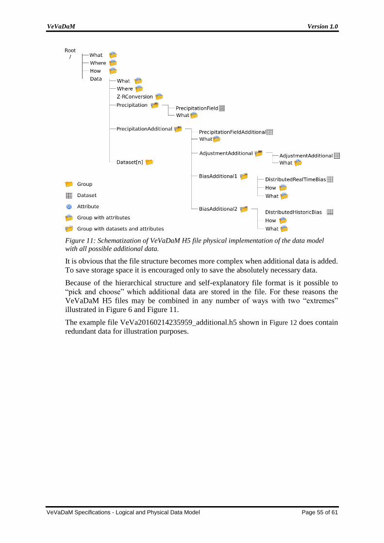
VeVaDaM Version 1.0


Figure 11: Schematization of VeVaDaM H5 file physical implementation of the data model

with all possible additional data.

It is obvious that the file structure becomes more complex when additional data is added.

To save storage space it is encouraged only to save the absolutely necessary data.

Because of the hierarchical structure and self-explanatory file format is it possible to

“pick and choose” which additional data are stored in the file. For these reasons the

VeVaDaM H5 files may be combined in any number of ways with two “extremes”

illustrated in Figure 6 and Figure 11.

The example file VeVa20160214235959_additional.h5 shown in Figure 12 does contain

redundant data for illustration purposes.

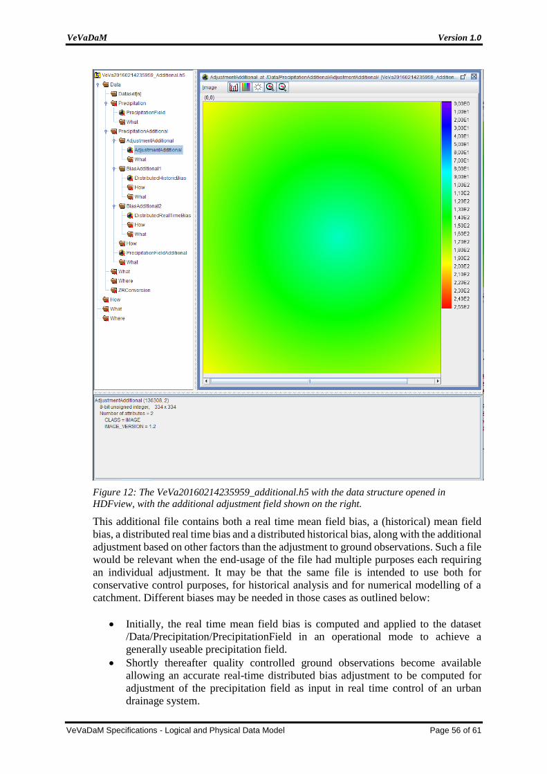
VeVaDaM Version 1.0


Figure 12: The VeVa20160214235959_additional.h5 with the data structure opened in

HDFview, with the additional adjustment field shown on the right.

This additional file contains both a real time mean field bias, a (historical) mean field

bias, a distributed real time bias and a distributed historical bias, along with the additional

adjustment based on other factors than the adjustment to ground observations. Such a file

would be relevant when the end-usage of the file had multiple purposes each requiring

an individual adjustment. It may be that the same file is intended to use both for

conservative control purposes, for historical analysis and for numerical modelling of a

catchment. Different biases may be needed in those cases as outlined below:

Initially, the real time mean field bias is computed and applied to the dataset

/Data/Precipitation/PrecipitationField in an operational mode to achieve a

generally useable precipitation field.

Shortly thereafter quality controlled ground observations become available

allowing an accurate real-time distributed bias adjustment to be computed for

adjustment of the precipitation field as input in real time control of an urban

drainage system.

VeVaDaM Version 1.0


The next day a distributed historical bias adjustment is computed based on the

overall bias adjustment need of several days of observations. This bias adjustment

is used for hindcast analysis purposes, such as analysis of intruding water,

hydraulic capacity, etc.

In this way, the file format does therefore support a number of different applications and

purposes.

The additional data added to this file relative to the minimum required data from the

preceding section are all located in the group “PrecipitationAdditional”. This group

inherits timestamps and geographical locations from the parent groups.

Figure 13: Meta-data attributes associated with the Data/PrecipitationAdditional group,

associated with all the datasets in the substructure.

The additional metadata located in /Data/PrecipitationAdditional/ are associated

specifically with the data contained in this group and its subgroups. The group

PrecipitationAdditional and the sub-groups How and What are shown in Figure 13 above

along with their attributes. The PrecipitationAdditional group defines the additional

mean field bias, the How group defines the attribute AppliedBias that defines which of

the available bias adjustments have been applied to the PrecipitationFieldAdditional. The

last attribute group is the What group which as for other datasets provides details of what

data are stored in the PrecipitationFieldAdditonal, ie. the gain/offset, Nodata and

Undetect value and the conversion factor from mm/hour to µm/s.

There are three subgroups with individual datasets under the PrecipitationAdditional,

namely the “AdjustmentAdditional”, the two distributed bias adjustments

“BiasAdditional1” and “BiasAdditional2”. Figure 14, shows the first three attribute

groups from this level. These are the attributes of the /AdjustmentAdditional/What group

and in the /BiasAdditional1/ the How and What sub-group respectively which contains

details of how the datasets were constructed and what is stored in them. For the

/BiasAdditional1/How the attribute BiasType1 defines the bias adjustment method used

to generate the dataset in this group – the DistributedHistoricBias. The What group

contains the usual gain/offset, along with details of what ground observations have been

VeVaDaM Version 1.0


used, and how they were applied – in this case the SVK5429 raingauge has been used

after removing spikes above 80 µm/s.

Figure 14: The /AdjustmentAddistional/What group along with the /BiasAdditional1/How and

What group associated with the PrecipitationAdditional group.

Finally, the How and What attribute groups of /BiasAdditional2/ is shown in Figure 15.

As this group is an alternative bias adjustment the information contained is very similar

to that stored in /BiasAdditional1/ shown in Figure 14. The main difference is that for

this adjustment dataset another method has been used – a realtime variant using 3 hours

of observations.

Figure 15: The /BiasAdditional2/How and What group associated with the

PrecipitationAdditional group.

VeVaDaM Version 1.0


Interpolated time step data structure

Walkthrough of the file: VeVa20160214235959_ Interpolated.h5

Using weighted 2D temporal interpolation between observed radar images it is possible

to create a pseudo-high temporal resolution. The VeVaDaM file structure supports this

interpolation, and an example file is provided from a C-band radar with a 10-minute

update interval. The data model is shown below in Figure 16.

Figure 16: Schematization of VeVaDaM H5 file physical implementation of the data model

with the minimum required data and interpolated radar images.

The structure in this file is as in the previous example an extension of the basic required

structure. In this case the basic structure – down to the PrecipitationField dataset in Figure

16 stores the measured, converted and mean-field bias adjusted precipitation field from

the C-band radar. The additional interpolated timesteps are all stored in the

/Data/Precipitation/ group. Again this can be combined in a number of ways with

additional bias and other adjustments in which case the same structure would have been

found in the /Data/PrecipitationAdditional/ group.

It is strongly encouraged to state the method and the pseudo-temporal resolution in the

/How/Interploation attribute and furthermore the timestep as a double in the attribute

/Precipitation/What/Interpolated_dt as shown in Figure 17.

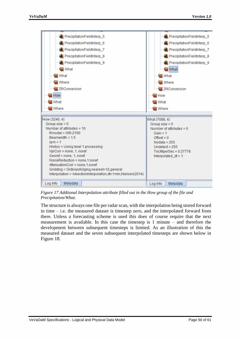
VeVaDaM Version 1.0


Figure 17 Addtional Interpolation attribute filled out in the How group of the file and

Precipitation/What.

The structure is always one file per radar scan, with the interpolation being stored forward

in time – i.e. the measured dataset is timestep zero, and the interpolated forward from

there. Unless a forecasting scheme is used this does of course require that the next

measurement is available. In this case the timestep is 1 minute – and therefore the

development between subsequent timesteps is limited. As an illustration of this the

measured dataset and the seven subsequent interpolated timesteps are shown below in

Figure 18.

VeVaDaM Version 1.0


Figure 18: In this HDFview screenshot the images are organized so that the upper left is the

measured dataset, and from left to right the subsequent 1 minute timesteps are shown, starting

with timestep +4 minutes in the second row.

Documents

VeVaDaM Weather Radar in the Water Sector · VeVaDaM Weather Radar in the Water Sector ... Refshalevej 250 1432 København K ... The documentation gives a short overview of the needed