Benchmarking is older. Simulation is more popular.But analytical queueing models may offer the most cost-effective

technique for computer system performance modeling.

QueueingModels ofComputerSystemsArnold 0. AllenIBM SystemsScience Institute

Figure 1 illustrates the spectrum of techniquesthat have been used for computer system perfor-mance modeling. The leftmost technique, the use ofsimple rules of thumb, is the easiest to apply and alsorequires the smallest investment of resources, whilethe rightmost technique, benchmarking, is the mostdifficult and costly.The rules of thumb range from simple, well-known

observations such as Murphy's law and Parkinson'slaw to some laws cited by Dickson' which have ob-vious applications to computer system performanceevaulation:Evie Nef's law. There is a solution to every prob-lem; the only difficulty is finding it.

Unnamed law. If it happens, it must be possible.Miller's law. You can't tell how deep a puddle is un-til you step into it.

Uhlmann 's razor. When stupidity is a sufficient ex-planation, there is no need to have recourse to anyother.

On a more prosaic level we have a few rules ofthumb developed by experience and recorded byR. M. Schardt2:

(1) Generally, channel utilization in direct accessstorage devices should not exceed 35 percentfor on-line applications or 40 percent for batchapplications.

(2) Individual DASD device utilizations shouldnot exceed 35 percent.

(3) Average arm seek time on a DASD deviceshould not exceed 50 cylinders.

(4) No block size for either tape or disk should beless than 4K bytes.

These rules of thumb were selected for computersoperating under control of the IBM MVS (multiplevirtual storages) operating system, but many perfor-mance analysts would agree that they are goodgeneral rules.Rules of thumb are excellent for day-to-day opera-

tion of computer installations but are not much helpin predicting hardware and software upgrading re-quirements. Linear projection of utilization and loadoffers a more organized approach. It requires measur-ing and tracking of such items as central processorutilization, channel utilization, communication lineutilization, etc., to establish growth rates for ex-trapolation. For reasonable effectiveness, the re-source requirements of applications under develop-ment must also be estimated. This technique is cer-tainly an improvement upon the rules-of-thumb tech-nique and, if properly implemented, can be a helpfulplanning tool. A major problem, however, is that thisapproach attempts to use linear prediction for sys-tems that are inherently nonlinear.

Simulation has been a very popular form of com-puter system modeling for years. It enables theanalyst to model the system at a much greater level of

0018-9162/80/0400-0013$00.75 C( 1980 IEEE 13April 1980

Vh6

detail than is practicable with queueing theorymodels. Unfortunately, simulation models are diffi-cult and costly to construct, validate, and run.Simulation projects tend to become large, long-term,and very difficult to control.t v X 9 k < -st W <1 S\ ., ~~~In terms of cost and complexity there is no sharpdistinction between simulation and benchmarking.Some simulation models are as complex and hard to

understand as the system being simulated! Likewise,abenchmark effort may be of rather limited scope,but if it is, it is probably nearly useless.The benchmarkingapproach to performance evalu-

ation is probably the oldest and most widely usedtechnique, although its use has been primarily fornew hardware selection. Thus, it is not a promisingtechnique for deciding when a hardware update is re-quired. The technique sounds disarmingly simple.You simply collect a representative sample of yourworkload, run it on the proposed machine, and mea-

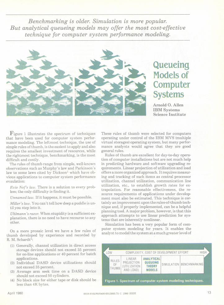
Figure 2. A typical queueing system. (Reprinted by permission of Xyzyx In- sure the performance. Unfortunately,all three offormation Corporation, Canoga Park, California.) sur th efrac. Unotnaey aUtreo

these tasks are very difficult in practice. Lucas3 gives*~~~~r.. ~~~~~~an excellent discussion of these difficulties as well as

_:.. a good explanation of simulation.One of the major benchmarking problems of recent

vintage has been that of generating the on-line com-ty, Staristics, adQeegTer SieRVeR 1pplicabons, ponent of the workload. In recent years this problem

has been greatly simplified by the emergence of thetype of program called a driver. This tool is ex-

SERVER2 - ~emplified by the IBM Teleprocessing Network Simu-lator.4

Figure 4. SomradomvarablsuednqeuengheoymdeA driver is a simulator which uses the actual orComputrplanned user-specified data communication network

(termiinals, lines, etc.) to model the network and toSERVERc ~ ~ generate and send messages to the computer system

under test, with a specific message mix and rate foreach terminal. Thus a driver can be used to approx-imate system performance and response times,

Figure 3. Elements of a queueing system.( Academic Press, Proba bili- evaluate communication network design, and testty, Statistics, and Queueing Theory with Computer Science Applications, new application programs. It may be less complex to1978)

Fiue4. oerno aibe sdi uuigter moe s.( A EaVemicPesPrbilt,Sasis,ndQuigThoywh

Copue Scec plctos 98

14 COMPUTER

use than some detailed simulation models but is ex-pensive in terms of hardware required.In the last two or three years the use of analytical

queueing models has become popular, although onlya few years ago simulation was the prevailing tech-nique. In 1978 an entire issue of ACM ComputingSurveys5 was devoted to queueing. Spragins6discusses the problems ofcomplex systems modelingand cites a number of cases showing how analyticalqueueing system models that are much simpler thanthe system modeled can beused successfully. This ar-ticle considers some analytical queueing theorymodels and shows how they can be used for perfor-mance modeling of computer systems. Most of theexamples are drawn from another work,7 where theyare discussed in greater depth.

Elements of queueing theory

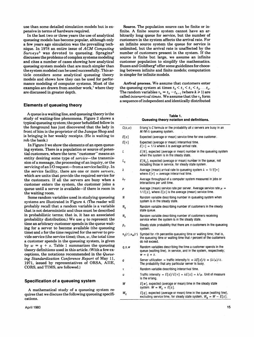
A queue is a waiting line, and queueing theory is thestudy of waiting-line phenomena. Figure 2 shows atypical queueing system; the poor befuddled fellow inthe foreground has just discovered that the lady infront of him is the proprietor of the Junque Shop andis bringing in her weekly receipts. (He is waiting torob the bank.)

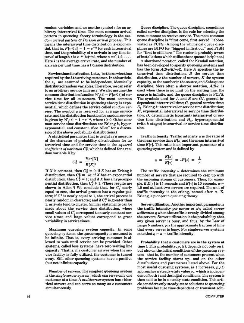
In Figure 3 we show the elements of an open queue-ing system. There is a population or source of poten-tial customers, where the term "customer" means anentity desiring some type of service-the transmis-sion of a message, the processing of an inquiry, or theservicing ofan I/O request-from a service facility. Inthe service facility, there are one or more servers,which are units that provide the required service forthe customers. If all the servers are busy when acustomer enters the system, the customer joins aqueue until a server is available-if there is room inthe waiting room.Some random variables used in studying queueing

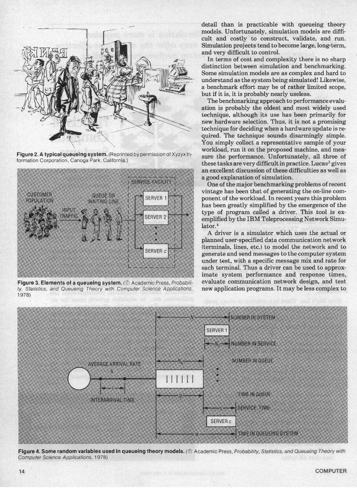
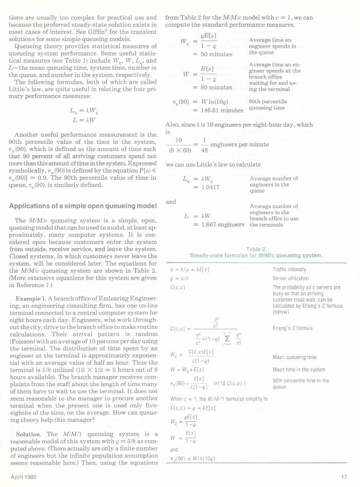
systems are illustrated in Figure 4. (The reader willprobably recall that a random variable is a variablethat is not deterministic and thus must be describedin probabilistic terms; that is, it has an associatedprobability distribution.) We use q to represent thetime an arbitrary customer spends in the queue wait-ing for a server to become available (the queueingtime) and s for the time required for the server to pro-vide service (the service time); thus, w, the total timea customer spends in the queueing system, is givenby w = q + s- Table 1 summarizes the queueingtheory definitions used in this article. (With a few ex-ceptions, the notations recommended in the Queue-ing Standardization Conference Report of May 11,1971, issued by representatives of ORSA, AIIE,CORS, and TIMS, are followed.)

Specification of a queueing system

A mathematical study of a queueing system re-quires thatwe discuss the following queueing specifi-cations.

Source. The population source can be finite or in-finite. A finite source system cannot have an ar-bitrarily long queue for service, but the number ofcustomers in the system affects the arrival rate. Foran infinite source system the queue for service isunlimited, but the arrival rate is unaffected by thenumber of customers present in the system. If thesource is finite but large, we assume an infinitecustomer population to simplify the mathematics.Buzen and Goldberg8 offer some guidelines for choos-ing between infinite and finite models; computationis simpler for infinite models.

Arrival process. We assume that customers enterthe queueing system at times to < t1 < t1 < t2 .. tn.The random variables Tk = tk-tk1 (where k > 1) arecalled interarrival times. We assume that the Tk forma sequence ofindependent and identically distributed

Table 1.Queueing theory notation and definitions.

C(c,u) Erlang's C formula or the probability all c servers are busy in anM/M/c queueing system.

E[s]E[T]

L

Expected (average or mean) service time for one customer.

Expected (average or mean) interarrival time.E[T] = 1 /A where A is average arrival rate.

E[N], expected (average or mean) number in the queueing systemwhen the system is in the steady state.

Lq E[Nq], expected (average or mean) number in the queue, notincluding those in service, for steady state system.

A Average (mean) arrival rate to queueing system A = 1/E[T]where E[T] = average interarrival time.

AT Average throughput of a computer system measured in jobs orinteractions per unit time.Average (mean) service rate per server. Average service rate , =1/E[s], where E[s] is the average (mean) service time.

N Random variable describing number in queueing system whensystem is in the steady state.

Nq Random variable describing number of customers in the steadystate queue.

Ns Random variable describing number of customers receivingservice when the system is in the steady state.

Pn Steady state probability that there are n customers in the queueingsystem.

TCq(r),nw(r) Symbol for rth percentile queueing time or waiting time; that is,the queueing time or waiting time that r percent of the customersdo not exceed.

q,s,w Random variables describing the time a customer spends in thequeue (waiting line), in service, and in the system, respectively;w = q + s.

Server utilization = traffic intensity/c = AE[s]/c = (A4s)/c.The probability that any particular server is busy.

T Random variable describing interarrival time.

u Traffic intensity = E[s]/E[T] -- E[s] = A4I*. Unit of measureis the erlang.

W E[w], expected (average or mean) time in the steady statesystem. W = Wq + E[s].

Wq E[q], expected (average or mean) time in the queue (waiting line),excluding service time, for steady state system. Wq = W - E[s].

April 1980 15

random variables, and we use the symbol T for an ar-bitrary interarrival time. The most common arrivalpattern in queueing theory terminology is the ran-dom arival pattern or Poisson arrival process. Thismeans the interarrival time distribution is exponen-tial, that is, P1[T < t] = 1e-At for each interarrivaltime, and the probability of n arrivals in any time in-tervalof length t is e-t(At) n/n!, where n = 0,1,2, . . .

Here A is the average arrival rate, and the number ofarrivals per unit time has a Poisson distribution.

Service time distribution. Let Sk be the service timerequired by the kth arriving customer. In this article,the sk are assumed to be independent, identicallydistributed random variables. Therefore, we can referto an arbitrary service time as s. We also assume thecommon distribution function W8(t) = P[s < t]of ser-vice time for all customers. The most commonservice-time distribution in queueing theory is expo-nential, which defines the service called random ser-vice. The symbol , is reserved for average servicerate, and the distribution function forrandom serviceis given by W8(t) = 1 -e-t, where t > 0. Other com-mon service time distributions are Erlang-k, hyper-eFponential, and constant. (See Allen7 for a discus-sion of the above probability distributions.)A statistical parameter that is useful as a measure

of the character of probability distributions for in-terarrival time and for service time is the squaredcoefficient of variation CQ, which is defined for a ran-dom variableX by

Var[XICX2 =

E[X]2IfX is constant, then Cx = 0; ifX has an Erlang-kdistribution, then Cx = 1lk; ifX has an exponentialdistribution, then Cx = 1; and ifX has a hyperexpo-nential distribution, then Cx > 1. (These results areshown in Allen.7) We conclude that, for C2 nearlyequal to zero, the arrival process has a regular pat-tern; if C2 is nearly equal to 1, the arrival process isnearly random in character; and if C 2 is greater than1, arrivals tend to cluster. Similar statements can bemade about the service time distribution, wheresmall values of Ce correspond to nearly constant ser-vice times and large values correspond to greatvariability in service times.

Maximum queueing system capacity. In somequeueing systems, the queue capacity is assumed tobe infinite. That is, every arriving customer is al-lowed to wait until service can be provided. Othersystems, called loss systems, have zero waiting linecapacity. That is, if a customer arrives when the ser-vice facility is fully utilized, the customer is turnedaway. Still other queueing systems have a positive(but not infinite) capacity.

Number of servers. The simplest queueing systemis the single-server system, which can serve only onecustomer at a time. A multiserver system has c iden-tical servers and can serve as many as c customerssimultaneously.

Queue discipline. The queue discipline, sometimescalled service discipline, is the rule for selecting thenext customer to receive service. The most commonqueue discipline is "first come, first served," abbre-viated as FCFS. (Among the whimsical queue disci-plines are BIFO for "biggest in first out" and FISHfor "first in still here." The reader is probably awareof installations which utilize these queue disciplines.)A shorthand notation, called the Kendall notation,

has been developed to specify queueing systems andhas the form A/B/c/K/m/Z. Here A specifies the in-terarrival time distribution, B the service timedistribution, c the number of servers, K the systemcapacity, m thenumber in the source, andZ the queuediscipline. More often a shorter notation, A/B/c, isused when there is no limit on the waiting line, thesource is infinite, and the queue discipline is FCFS.The symbols used for A and B are GI, general in-dependent interarrival time; G, general service time;Ek, Erlang-k interarrival or service time distribution;M, exponential interarrival or service time distribu-tion; D, deterministic (constant) interarrival or ser-vice time distribution; and H", hyperexponential(with k stages) interarrival or service time distribu-tion.

Traffic intensity. Traffic intensity u is the ratio ofthe mean service timeE[s] and the mean interarrivaltime ElT]. This ratio is an important parameter of aqueueing system and is defined by

U = E[s] = E[sE[Tl

The traffic intensity u determines the minimumnumber of servers that are required to keep up withthe incoming stream of customers. Thus, for exam-ple, if E(s] is 15 seconds and E[Tj is 10 seconds, u =1.5 and at least two servers are required. The unit oftraffic intensity is the erlang, named after A. K.Erlang, a pioneer in queueing theory.

Server utilization. Another important parameter isthe traffic intensity per server or u/, called serverutilization Q when the traffic is evenly divided amongthe servers. Server utilization is the probability thatany given server is busy, and thus, by the Law ofLarge Numbers, Q is the approximate fraction of timethat every server is busy. For single-server systemsnote that Q = u = traffic intensity.

Probability that n customers are in the system attime t. This probability, Pn (t), depends not only on t,but also on the initial conditions of the queueing sys-tem-that is, the number of customers present whenthe service facility starts up-and on the otherdistributions and parameters listed above. For themost useful queueing systems, as t increases, pn(t)approaches a steady-state valuepn, wh:ich is indepen-dent ofboth t and the initial conditions. The system isthen said to be in a steady-state condition. This arti-cle considers only steady-state solutions to queueingproblems because time-dependent or transient solu-

COMPUTER16

tions are usually too complex for practical use andbecause the preferred steady-state solution exists inmost cases of interest. See Giffin9 for the transientsolutions for some simple queueing models.Queueing theory provides statistical measures of

queueing system performance. Some useful statis-tical measures (see Table 1) include Wq, W, Lq, andL-the mean queueing time, system time, number inthe queue, and number in the system, respectively.The following formulas, both of which are called

Little's law, are quite useful in relating the four pri-mary performance measures:

Lq =JlWq

L =W

Another useful performance measurement is the.90th percentile value of the time in the system,nT(90), which is defined as the amount of time suchthat 90 percent of all arriving customers spend notmore than this amount oftime in the system. Expressedsymbolically, iT.(90) is defined by the equationP[w <nw(90)] = 0.9. The 90th percentile value of time inqueue, 7Tq(90), is similarly defined.

Applications of a simple open queueing model

The M/M/c queueing system is a simple, open,queueing model that can be used to model, at least ap-proximately, many computer systems. It is con-sidered open because customers enter the systemfrom outside, receive service, and leave the system.Closed systems, in which customers never leave thesystem, will be considered later. The equations forthe MIMIc queueing system are shown in Table 2.(More extensive equations for this system are givenin Reference 7.)

Example 1. A branch office of Endearing Engineer-ing, an engineering consulting firm, has one on-lineterminal connected to a central computer system foreight hours each day. Engineers, who work through-out the city, drive to the branch office to make routinecalculations. Their arrival pattern is random(Poisson) with an average of 10 persons per day usingthe terminal. The distribution of time spent by anengineer at the terminal is approximately exponen-tial with an average value of half an hour. Thus theterminal is 5/8 utilized (10 X 1/2 = 5 hours out of 8hours available). The branch manager receives com-plaints from the staff about the length of time manyof them have to wait to use the terminal. It does notseem reasonable to the manager to procure anotherterminal when the present one is used only five-eighths of the time, on the average. How can queue-ing theory help this manager?

Solution. The M/M/1 queueing system is areasonable model of this system with Q = 5/8 as com-puted above. (There actually are only a finite numberof engineers but the infinite population assumptionseems reasonable here.) Then, using the equations

from Table 2 for the M/M/c model with c = 1, we cancompute the standard performance measures.

QE[s]Wq - e

= 50 minutes

E[s]

1 -Q= 80 minutes

Average time anengineer spends inthe queue

Average time an en-gineer spends at thebranch officewaiting for and us-ing the terminal

lTq(90) = Wln(1OQ) 90th percentile= 146.61 minutes queueing time

Also, since A is 10 engineers per eight-hour day, whichis

10 _110 = - engineers per minute(8 X 60) 48

we can use Little's law to calculate

Lq = lWq= 1.0417

and

Average number ofengineers in thequeue

Average number ofengineers in theL = AW branch office to use

= 1.667 engineers the terminals

Table 2.Steady-state formulas for MIMIc queueing system.

u = AI/ = AE[s]Q = U/C

C(c, u)

uc

C(c,u) c!UC c-1 Un-4(1-Q) E -

c! n=O n!

Wq = C(c,u)E[s]c( -Q)

W = Wq+E[s]

90)= Ec( se) In(10 C(c,u) )

When c = 1, the M/M/1 formulas simplify to

C(c,u) Q = XE[s]

QE[s]Wq 1 -Q

E[s]w

1 -

and

Tr,(90) = Win(10).

Traffic intensityServer utilizationThe probability all c servers arebusy so that an arrivingcustomer must wait; can becalculated by Erlang's C formula(below)

Erlang's C formula

Mean queueing time

Mean time in the system

90th percentile time in thequeue

April 1980

These statistics show that slightly more than oneengineer-day is being lost by engineers queueing upto use the terminal. In the next example we will seehow theM/M/c queueing system model can be used tomake an informed decision on how to solve the prob-lem.

Example 2. In Example 1 we discovered a puzzlingsituation at Endearing Engineering. Although theirremote terminal was only 62.5 percent utilized, theaverage time an engineer had to queue for the ter-minal was 50 minutes with 10 percent of them havingto wait for over 146.61 minutes. A committee ofengineers met with the branch manager and showedhow queueing theory could explain what was happen-ing. They decided the problem could not be solved byscheduling terminal time; one or more additional ter-minals should be provided. They specified that themean queueing time should not exceed 10 minuteswith the 90th percentile value of queueing time not toexceed 15 minutes. Thebranch manager then had sec-ond thoughts; he reasoned that, if the average queue-ing time is 50 minutes with one terminal, then it mustbe 25 minutes with two terminals, and thus five ter-minals would be required to make Wq < 10 minutes.How many terminals are required?

'Solution. The solution, of course, depends uponwhether all the terminals are installed at the branchoffice, giving one MIMIc queueing system, or aredistributed to several customer locations, thus pro-viding multiple single-server (M/M/1) queueing sys-tems. Let us consider the former case first, by trying c= 2, that is, providing two terminals in the branch of-fice. (We are motivated, in part, by the fact that theequations are much easier to solve for c = 2 than for c-5.)

Q =0.625/2 .Server utilization= 0.3125

C(2,u) = C(2,0.625) Probability both= 0.1488 servers are busy

C(c, u)Es]W C Mean time in the

Wq c(1 - Q) queue= 3.247 minutes

E[s]nq(90) - ln(10 C(c,u)) 90th percentilec( -Q) queueing timne

= 8.67 minutes

Thus one additional terminal in the branch office willsatisfy all the requirements.

If the additional terminal is placed at a customierlocation and the traffic to the two terminals is evenlysplit, there would be two M/M/1 queueing systems,each with Q = 0.3125. Then, by the formulas of Table2, for c = 1, we calculate

QEsWq =

= 13.64 minutesMean queueing time

E[s]Trq(90) = ln (1OQ)

1 -Q= 49.72 minutes.

90th percentilequeueing time

Thus two distributed terminals will not meet either ofthe criteria.Table 3 shows the results for various numbers of

terminals. Some, rising above principle, might decideto settle for four distributed terminals; however, thestated criteria mean that, if the terminals are dis-persed, five are required. Thus the branch manager isright. (It's not nice to fool your manager!) We havenot, of course, considered the travel time forengineers to reach a terminal. Using queueing theorymodels and cost information concerning travel timeto the terminals, it is possible to determine the mostcost effective solution to the problem. (For an exam-ple, see Reference 7, Chapter 5, Exercise 13.)

Finite population queueing models ofinteractive computer systems

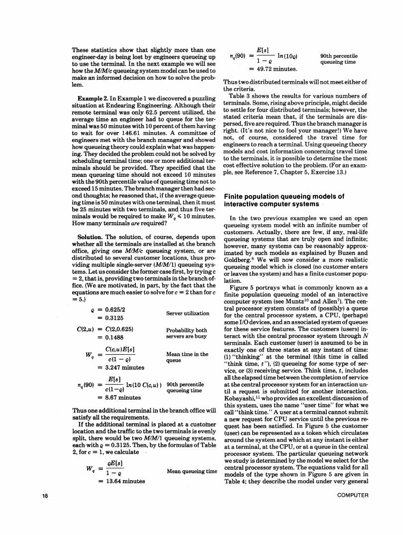
In the two previous examples we used an openqueueing system model with an infinite number ofcustomers. Actually, there are few, if any, real-lifequeueing systems that are truly open and infinite;however, many systems can be reasonably approx-imated by such models as explained by Buzen andGoldberg.8 We will now consider a more realisticqueueing model which is closed (no customer entersor leaves the system) and has a finite customer popu-lation.Figure 5 portrays what is commonly known as a

finite population queueing model of an interactivecomputer system (see Muntz'0 and Allen7). The cen-tral processor system consists of (possibly) a queuefor the central processor system, a CPU, (perhaps)some I/O devices, and an associated system of queuesfor these service features. The customers (users) in-teract with the central processor system through Nterminals. Each customer (user) is assumed to be inexactly one of three states at any instant of time:(1) "thinking" at the terminal (this time is called"think time, t"), (2) queueing for some type of ser-vice, or (3) receiving service. Think time, t, includesall the elapsed time between the completion of serviceat the central processor system for an interaction un-til a request is submitted for another interaction.Kobayashi,1I who provides an excellent discussion ofthis system, uses the name "user time" for what wecall "think time." A user at a terminal cannot submita new request for CPU service until the previous re-quest has been satisfied. In Figure 5 the customer(user) can be represented as a token which circulatesaround the system and which at any instant is eitherat a terminal, at the CPU, or at a queue in the centralprocessor system. The particular queueing networkwe study is determined by the model we select for thecentral processor system. The equations valid for allmodels of the type shown in Figure 5 are given inTable 4; they describe the model under very general

COMPUTER18

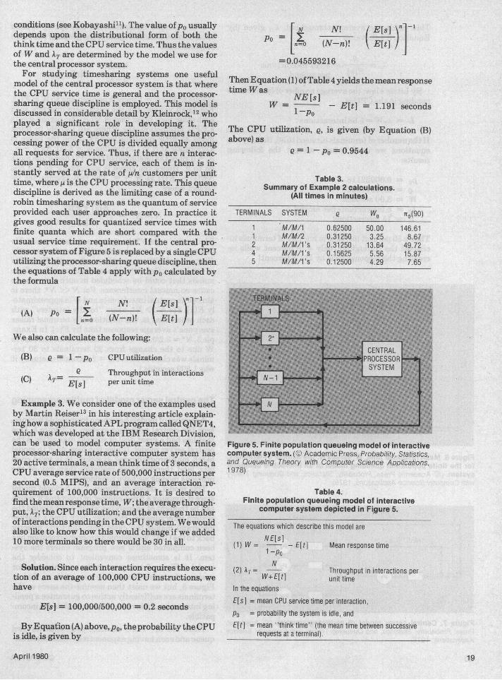
conditions (see Kobayashi'1). The value ofpo usuallydepends upon the distributional form of both thethink time and the CPU service time. Thus the valuesof W and AT are determined by the model we use forthe central processor system.For studying timesharing systems one useful

model of the central processor system is that wherethe CPU service time is general and the processor-sharing queue discipline is employed. This model isdiscussed in considerable detail by Kleinrock,12 whoplayed a significant role in developing it. Theprocessor-sharing queue discipline assumes the pro-cessing power of the CPU is divided equally amongall requests for service. Thus, if there are n interac-tions pending for CPU service, each of them is in-stantly served at the rate of p/n customers per unittime, where p is the CPU processing rate. This queuediscipline is derived as the limiting case of a round-robin timesharing system as the quantum of serviceprovided each user approaches zero. In practice itgives good results for quantized service times withfinite quanta which are short compared with theusual service time requirement. If the central pro-cessor system of Figure 5 is replaced by a single CPUutilizing the processor-sharing queue discipline, thenthe equations of Table 4 apply with po calculated bythe formula

N

(A) Po =ln=O

N!(Nn)!

N!Po = jjb (N-n)!

=0.045593216

E[s]n -1

\E[t]/|

Then Equation (1) ofTable 4 yields themean responsetime W as

NE[s]W = - E[t] = 1.191 seconds

1 -Po

The CPU utilization, Q, is given (by Equation (B)above) as

Q = -po = 0.9544

Table 3.Summary of Example 2 calculations.

(All times in minutes)

TERMINALS SYSTEM Q Wq nq(90)1 M/M/1 0.62500 50.00 146.611 M/M/2 0.31250 3.25 8.672 M/M/1's 0.31250 13.64 49.724 M/M/1's 0.15625 5.56 15.875 M/M/1's 0.12500 4.29 7.65

IE[s]E[t] fl

We also can calculate the following:

(B) Q = 1 -po CPU utilizationQ Throughput in interactions

(C) AT= E[s] unit tiime

Example 3. We consider one of the examples usedby Martin Reiser13 in his interesting article explain-inghow a sophisticated APLprogram calledQNET4,which was developed at the IBM Research Division,can be used to model computer systems. A finiteprocessor-sharing interactive computer system has20 active terminals, a mean think time of 3 seconds, aCPU average service rate of 500,000 instructions persecond (0.5 MIPS), and an average interaction re-quirement of 100,000 instructions. It is desired tofind the mean response time, W; the average through-put, AT; the CPU utilization; and the average numberofinteractions pending in theCPU system. We wouldalso like to know how this would change if we added10 more terminals so there would be 30 in all.

Solution. Since each interaction requires the execu-tion of an average of 100,000 CPU instructions, wehave

E[s] = 100,000/500,000 = 0.2 seconds

By Equaiion (A) above,po, the probability the CPUis idle, is given by

Figure 5. Finite population queueing model of interactivecomputer system. (© Academic Press, Probability, Statistics,and Ququeing Theory with Computer Science Applications,1978)

Table 4.Finite population queueing model of interactive

computer system depicted in Figure 5.

The equations which describe this model areN E[S]I

(1) W = - - E[t]1 -PON

(2)AT= -W+E[t]

In the equations

Mean response time

Throughput in interactions perunit time

E[SI = mean CPU service time per interaction,po = probability the system is idle, andE[t] = mean think time" (the mean time between successive

requests at a terminal).

April 1980 19

This yields the average throughput, AT, given (byEquation (C) above) as

eAT = = 4.722 interactions

E[s] per second

By Little's law, the average number of interactionspending in the CPU is

L = ATW= 5.68 interactions

If the number of terminals is raised to 30, then, by theequations we used before, we get the followingresults:

po = 0.00022118Q = 0.99977882W = 3.00 secondsAT = 5 interactions per secondL = 15 interactions

Thus a 50 percent increase in number of terminals in-creased the throughput only 4.78 percent while in-creasing the response time by 151.9 percent!

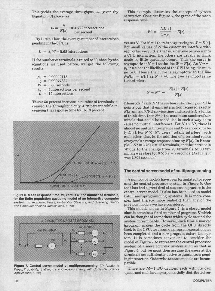
Figure 6. Mean response time, W, versus N, the number of terminals,for the finite population queueing model of an interactive computersystem. (© Academic Press, Probability, Statistics, and Queueing Theorywith Computer Science Applications, 1978)

Figure 7. Central server model of multiprogramming. (© AcademicPress, Probability, Statistics, and Queueing Theory with Computer ScienceApplications, 1978)

This example illustrates the concept of systemsaturation. Consider Figure 6, the graph of the meanresponse time

NE[s]rW - --E[t]

versusN. ForN= 1 there is no queueing soW=E [s].For small values of N the customers interfere witheach other very little; that is, when one person wantsa CPU interaction, the others are usually in thinkmode so little queueing occurs. Thus the curve isasymptotic atN= lto the line W =Es. AsN-'- 0,po - 0 since the likelihood of theCPU being idle mustgo to 0. Hence the curve is asymptotic to the lineNE[s] - E[t] as N - . The two asymptotes in-tersect where

E[s] +E[t]N=N* = E[s

Kleinrock12 calls N* the system saturationpoint. Hepoints out that, if each interaction required exactlyE[s] units ofCPU service time andexactlyE[t] unitsof think time, thenN* is themaximum number of ter-minals that could be scheduled in such a way as tocause no mutual interference. For N << N*, there isalmost no mutual interference and Wis approximate-ly E[s]. For N >> N*, users "totally interfere" witheach other; that is, the addition of a terminal raiseseveryone's average response time byE [s ]. In Exam-ple 3, N* = 3.2/0.2 = 16 terminals, and the increase inW due to the change from 20 terminals to 30 ter-minals was close to 10 X 0.2 = 2 seconds. (Actually itwas 1.809 seconds.)

The central server model of multiprogramming

A number ofmodels have been formulated to repre-sent the central processor system in Figure 5. Onethat has had a great deal of success in practice is thecentral server model. It also has been used to modelbatch multiprogramming systems. It is more com-plex (and thereby more realistic) than any of theprevious models we have considered.This model, shown in Figure 7, is a closed model

since it contains a fixed number of programsK whichcan be thought of as markers which cycle around thesystem interminably. However, each time a marker(program) makes the cycle from the CPU directlyback to the CPU, we assume,a program execution hasbeen completed and a new program enters the sys-tem. It is sometimes convenient to consider themodel of Figure 7 to represent the central processorsystem of a more complex system such as that inFigure 5, but we must then assume the users at theterminals are sufficiently active to guarantee a pend-ing interaction. Otherwise the two models are incom-patible.There are M-1 I/O devices, each with its own

queue and each having exponentially distributed ser-

COMPUTER20

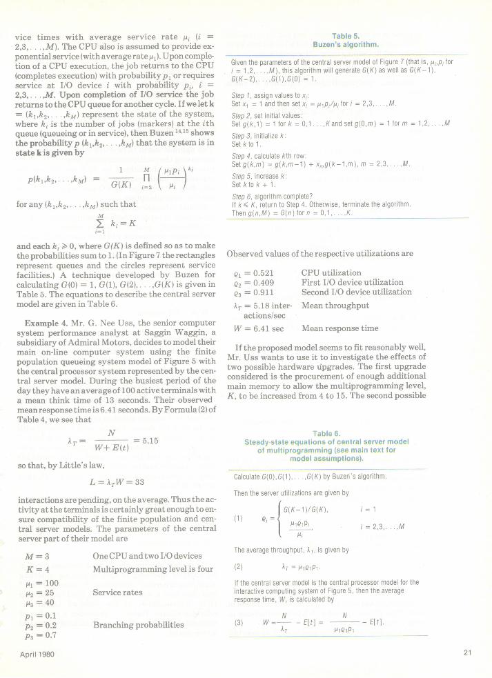
vice times with average service rate IA (i =2,3,. . .,M). The CPU also is assumed to provide ex-ponential service (with average rate I). Upon comple-tion of a CPU execution, the job returns to the CPU(completes execution) with probability Pi or requiresservice at I/O device i with probability pi, i =2,3,. . ,M. Upon completion of I/O service the jobreturns to theCPU queue for another cycle. Ifwe let k= (k1,k2,. . .,km) represent the state of the system,where ki is the number of jobs (markers) at the ithqueue (queueing or in service), then Buzen 14,15 showsthe probability p (k1,k2, .,kM) that the system is instate k is given by

I M I YPii \ i

p(k1,k2. ,M) = -G(K) in2 )

for any (kl,k2,. .,kM) such thatM

z ki=Ki=l

and each k, > 0, where G(K) is defined so as to makethe probabilities sum to 1. (In Figure 7 the rectanglesrepresent queues and the circles represent servicefacilities.) A technique developed by Buzen forcalculating G(0) = 1, G(1), G(2),. . .,G(K) is given inTable 5. The equations to describe the central servermodel are given in Table 6.

Example 4. Mr. G. Nee Uss, the senior computersystem performance analyst at Saggin Waggin, asubsidiary of Admiral Motors, decides to model theirmain on-line computer system using the finitepopulation queueing system model of Figure 5 withthe central processor system represented by the cen-tral server model. During the busiest period of theday they have an average of 100 active terminals witha mean think time of 13 seconds. Their observedmean response time is 6.41 seconds. By Formula (2) ofTable 4, we see that

NAT=r = 5.15

W+ E(t)

so that, by Little's law,

L=ATW=33

interactions are pending, on the average. Thus the ac-tivity at the terminals is certainly great enough to en-sure compatibility of the finite population and cen-tral server models. The parameters of the centralserver part of their model are

Table 5.Buzen's algorithm.

Given the parameters of the central server model of Figure 7 (that is, j'i,p fori = 1,2,. M), this algorithm will generate G(K) as well as G(K-1),G(K-2),. G(l ),G(O) = 1.

Step 1, assign values to xi:Set x, = 1 and then set xi = IAip,l' for i = 2,3, . , M.

Step 2, set initial values:Set g(k,1) = 1 for k = 0,1. ,Kand set g(O,m) = 1 for m = 2,.,,M

Step 3, initialize k:Set k to 1.Step 4, calculate kth row:Set g(k,m) = g(k,m-1) + x,g(k-1 ,m), m = 2,3,. M.

Step 5, increase k:Set kto k + 1.

Step 6, algorithm complete?If k < K, return to Step 4. Otherwise, terminate the algorithm.Then g(n,M) = G(n) for n = 0,1,. K.

Observed values of the respective utilizations are

Q, = 0.521Q2 = 0.409Q3 = 0.911

CPU utilizationFirst I/O device utilizationSecond I/O device utilization

1T = 5.18 inter- Mean throughputactions/sec

W = 6.41 sec Mean response time

If the proposed model seems to fit reasonably well,Mr. Uss wants to use it to investigate the effects oftwo possible hardware upgrades. The first upgradeconsidered is the procurement of enough additionalmain memory to allow the multiprogramming level,K, to be increased from 4 to 15. The second possible

Table 6.Steady-state equations of central server model

of multiprogramming (see main text formodel assumptions).

Calculate G(0),G(1), G(K) by Buzen's algorithm.

Then the server utilizations are given by

G(K-1)/G(K),( Qi i ltQi P,

Pi

i = 1

OneCPU andtwo I/O devicesMultiprogramming level is four

Service rates

Branching probabilities

The average throughput, AT, is given by

(2) AT = MlQiPliIf the central server model is the central processor model for theinteractive computing system of Figure 5, then the averageresponse time, W, is calculated by

N N(3) W= - E[t] = - E[t].ArT HAQPI

M=3K=4

f', = 100P2 = 25A3 = 40

pI = 0.1P2 = 0.2P3 = 0.7

April 1980

upgrade is to make hardware and software changeswhich will effectively speedup both I/O devices by 25percent while keeping the multiprogramming level atfour.

Solution. Applying Buzen's Algorithm we calcu-late

xl= 1,x2 =Ml1P24'2 =0.8

and

the IIO devices are 25 percent faster, Mr. Uss'scalculations show similarly that

el = 0.616300129Q2 = 0.394432082Q3= 0.862820181= 6.163 interactions per second

and

W = 3.226 seconds

X3= lJP31IA3 = 1.75

Continuing with Buzen's algorithm yields the follow-ing table for the original model:

Xl X21 0.8

0 1 11 1 1.82 1 2.443 1 2.9524 1 3.3616

X3

1.751 = G(0)3.55 = G(1)8.6525 = G(2)18.093875 = G(3)35.02588125 = G(4) = G(K)

This upgrade seems to be much more favorable thanincreasing the multiprogramming level to 15. It im-proves mean throughput by 19.3 percent and de-creases the mean response time by 49.3 percent. Italso does not overload the I/O devices as heavily asthe first upgrade option.Similar calculations can also show Mr. Uss the im-

provement to expect if both of the upgrades are donesimultaneously, that is, if we get faster I/O devicesand enough main memory to raise the multiprogram-ming level to 15. This would give a great deal of im-provement. Mr. Uss calculates that

Then, by the equations of Table 6,

Q, = G(3)/G(4) = 0.51658586 CPUutilization

Q2 PlQ1P24'2- 0.413268688

Q3 = lAlQ1P3/IA3= 0.904025256

AT = lAl= 5.1658586 interactions

per second

W= --E[t]63T 6

= 6.357866 seconds

Utilization of firstI/O device

Utilization of sec-ond I/O device

Mean throughput

Mean responsetime

These values are certainly close enough to themeasured values to validate the model. Mr. Ussshould proceed.minilar calculations show that if the multiprogram-

ming level is increased to 15 from 4, then

=0.571282414Q2 =0.457025931Q= 0.999744225AT= 5.71282 interactions per second

and

W =4.505 seconds

Thus, there has been a 10.6 percent improvement inmean throughput, AT, and a 29.2 percent decrease inmean response time, W.

If the multiprogramming level is kept at four but

22

AT = 7.123 interactions per second

and

W = 1.039 seconds

This is a 15.6 percent improvement in mean through-put and a 67.8 percent decrease in the mean responsetime over the system with faster I/O devices but withthe multiprogramming level kept at four. Comparedto the original system it showsa 24.7 percent increasein AT and a 76.9 percent decrease in W.The reader should note that what we have glibly

represented as an I/O device may very well be repre-sented in physical hardware by a block multiplexerchannel with several attached disk drives in the caseof the first I/O device, and by such a channel withseveral drums in the case of the second I/O device.

If the first I/O device on the original system is re-placed by one with the same speed as the second I/Odevice, and the load on the two devices is balanced sothat the branching probability to each is 0.45, thenwe would have

T= 6.14 interactions per second

and

W = 3.285 seconds

The central server model is one of themost success-ful analytic queueing models in use for modelingmultiprogramming computer systems. Price16describes how it was successfully used to model anIBM System/360-91 at the Stanford Linear Ac-celerator Center. Buzen'7"8 describes a number ofsuccessful modeling efforts which utilized the centralserver model.

COMPUTER

Some useful approximations

Many computer systems can be modeled as a "net-work of queues," that is, a network of simple queue-ing systems in which the input(s) toone queueing sys-tem may be output(s) from one or more other queue-ing system(s). Unfortunately little can be done,analytically, with general queueing networks, exceptin the simple case covered by Jackson's theorem (seeAllen7) in which al elements of the network areMIMIc queueing systems and all arrival patterns arerandom (Poisson). However, there are some simpleapproximations which can be used to model fairlycomplex queueing networks.One useful approximation noted by the author and

his colleague, John Cunneen, can be stated (modest-ly) as the Allen-Cunneen approximation formula. Forany GI/Gic queuemg system it is approximately truethat

C(c,u)E[s] {,C+ C.,

In this formnula, C(c,u) is Erlang's C formul (shownin Table 2); Cc,is the squared coefficient of vari-ation for the interarrival time and service time,respectively; and Q is the server utilization. A similar,but slightly more complex formula for the singleserver case has been given by Kuehn.19 The approx-imation formula above is exact for MIMIc and M/G/1queueing systems and gives a reasonably good ap-proximation for many others. Examples of its use aregiven in Allen. It is easy to compute, and the furtherapproximation

C(c,u) QC

(E)c(l-Q) l -Qc

can be used to make the computation even easier.Equation (E) is exact for c = 1,2 but is a little low forother values of c.

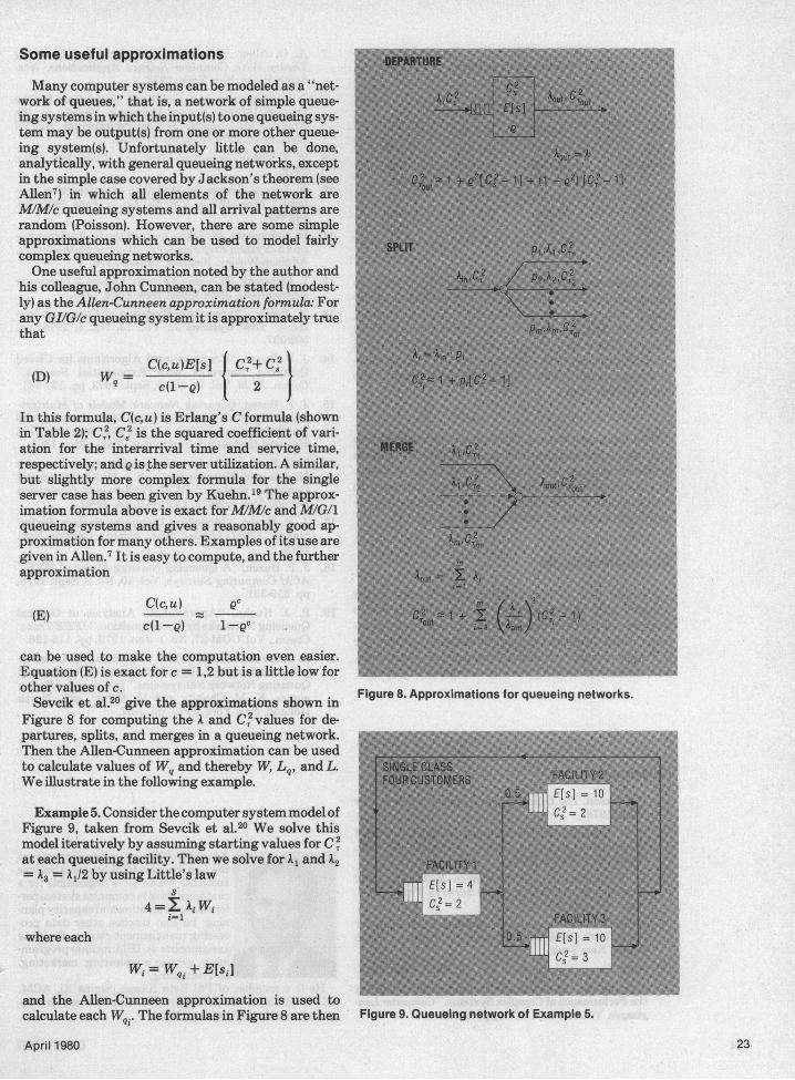
Sevcik et al.20 give the approximations shown in Figure 8. Approximations for queueing netFigure 8 for computing the A and CT values for de-partures, splits, and merges in a queueing network.Then the Allen-Cunneen approximation can be usedto calculate values of Wq and thereby W, Lg, and L.We illustrate in the folowing example.1Example 5. Consider the computer system model of Cs'= 2

Figure 9, taken from Sevcik et al.20 We solve thismodel iteratively by assuming starting values for CTat each queueing facility. Then we solve for A1 and A2= A3 = A1I2 by using Little's law

8' 3 _I7l ET s ]~~~C=2 _

4= AiWi

where each ES

Wi =WjW + E[si]

and the Allen-Cunneen approximation is used tocalculate each W.,. The formulas in Figure 8 are then Figure 9. Queueing network of Example 5.

works.

April 1980 23

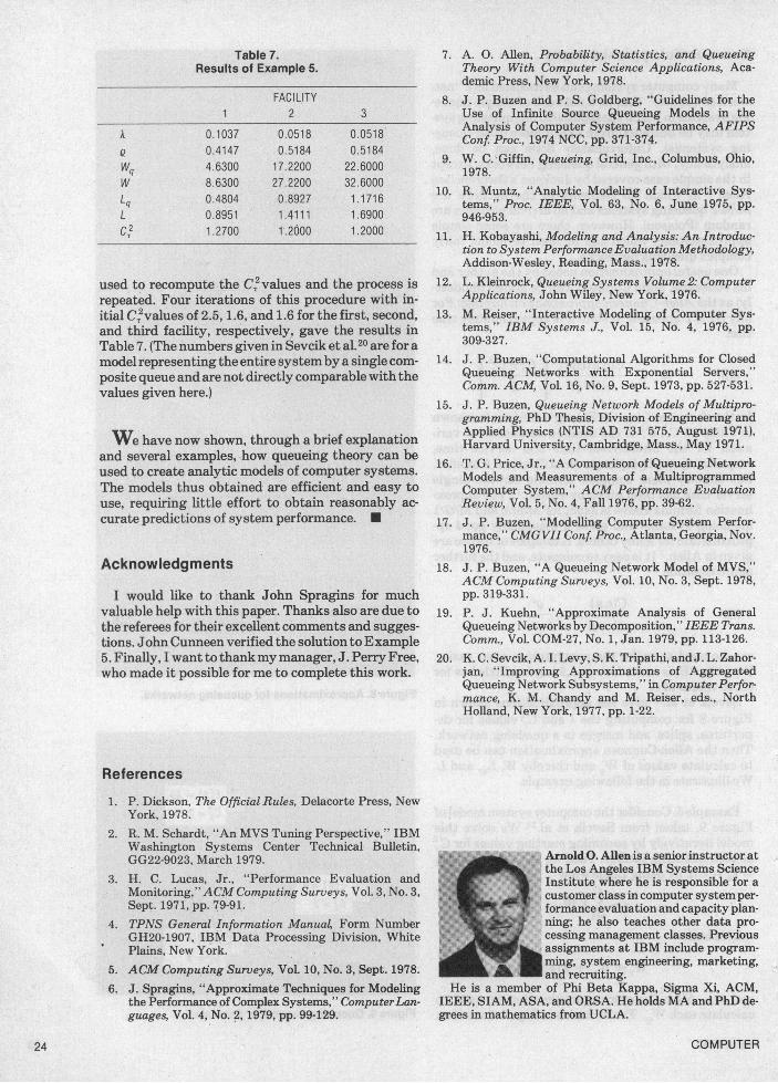
Table 7.Results of Example 5.

FACILITY1 2 3

A 0.1037 0.0518 0.0518Q 0.4147 0.5184 0.5184Wq 4.6300 17.2200 22.6000W 8.6300 27.2200 32.6000Lq 0.4804 0.8927 1.1716L 0.8951 1.4111 1.6900

TC2 1.2700 1.2000 1.2000

used to recompute the C2values and the process isrepeated. Four iterations of this procedure with in-itial C 2values of 2.5, 1.6, and 1.6 for the first, second,and third facility, respectively, gave the results inTable 7. (The numbers given in Sevcik et al.20 are for amodel representing the entire systemby a single com-posite queueand are not directly comparablewith thevalues given here.)

We have now shown, through a brief explanationand several examples, how queueing theory can beused to create analytic models of computer systems.The models thus obtained are efficient and easy touse, requiring little effort to obtain reasonably ac-curate predictions of system performance. M

Acknowledgments

I would like to thank John Spragins for muchvaluable help with this paper. Thanks also are due tothe referees for their excellent comments and sugges-tions. John Cunneen verified the solution toExample5. Finally, I want tothankmymanager, J. Perry Free,who made it possible for me to complete this work.

References

1. P. Dickson, The Official Rules, Delacorte Press, NewYork, 1978.

2. R. M. Schardt, "An MVS Tuning Perspective," IBMWashington Systems Center Technical Bulletin,GG22-9023, March 1979.

3. H. C. Lucas, Jr., "Performance Evaluation andMonitoring,"ACM Computing Surveys, Vol. 3, No. 3,Sept. 1971, pp. 79-91.

4. TPNS General Information Manual, Form NumberGH20-1907, IBM Data Processing Division, WhitePlains, New York.

5. ACM Computing Surveys, VoL 10, No. 3, Sept. 1978.6. J. Spragins, "Approximate Techniques for Modeling

the Performance of Complex Systems," ComputerLan-guages, Vol. 4, No. 2, 1979, pp. 99-129.

7. A. 0. Allen, Probability, Statistics, and QueueingTheory With Computer Science Applications, Aca-demic Press, New York, 1978.

8. J. P. Buzen and P. S. Goldberg, "Guidelines for theUse of Infinite Source Queueing Models in theAnalysis of Computer System Performance, AFIPSConf. Proc., 1974 NCC, pp. 371-374.

9. W. C. Giffin, Queueing, Grid, Inc., Columbus, Ohio,1978.

10. R. Muntz, "Analytic Modeling of Interactive Sys-tems," Proc. IEEE, Vol. 63, No. 6, June 1975, pp.946-953.

11. H. Kobayashi, Modeling and Analysis: An Introduc-tion to System PerformanceEvaluationMethodology,Addison-Wesley, Reading, Mass., 1978.

12. L. Kleinrock, Queueing Systems Volume 2: ComputerApplications, John Wiley, New York, 1976.

13. M. Reiser, "Interactive Modeling of Computer Sys-tems," IBM Systems J., Vol. 15, No. 4, 1976, pp.309-327.

14. J. P. Buzen, "Computational Algorithms for ClosedQueueing Networks with Exponential Servers,"Comm. ACM, Vol. 16, No. 9, Sept. 1973, pp. 527-531.

15. J. P. Buzen, Queueing Network Models of Multipro-gramming, PhD Thesis, Division of Engineering andApplied Physics (NTIS AD 731 575, August 1971),Harvard University, Cambridge, Mass., May 1971.

16. T. G. Price, Jr., "A Comparison of Queueing NetworkModels and Measurements of a MultiprogrammedComputer System," ACM Performance EvaluationReview, Vol. 5, No. 4, Fall 1976, pp. 39-62.

17. J. P. Buzen, "Modelling Computer System Perfor-mance," CMG VII Conf Proc., Atlanta, Georgia, Nov.1976.

18. J. P. Buzen, "A Queueing Network Model of MVS,"ACM Computing Surveys, Vol. 10, No. 3, Sept. 1978,pp. 319-331.

19. P. J. Kuehn, "Approximate Analysis of GeneralQueueing Networks by Decomposition, " IEEE Trans.Comm., Vol. COM-27, No. 1, Jan. 1979, pp. 113-126.

20. K. C. Sevcik, A. I. Levy, S. K. Tripathi and J. L. Zahor-jan, "Improving Approximations of AggregatedQueueing Network Subsystems," in ComputerPerfor-mance, K. M. Chandy and M. Reiser, eds., NorthHolland, New York, 1977, pp. 1-22.

Arnold 0. AlUen is a senior instructor atthe Los Angeles IBM Systems ScienceInstitute. where he is responsible for acustomer class in computer system per-formance evaluation and capacity plan-ning; he also teaches other data pro-cessing management classes. Previousassignments at IBM include program-ming, system engineering, marketing,and recruiting.

He is a member of Phi Beta Kappa, Sigma Xi, ACM,IEEE, SIAM, ASA, and ORSA. He holds MA and PhD de-grees in mathematics from UCLA.

COMPUTER24