Embed Size (px)
Citation preview
VHDL IMPLEMENTATION OF
REED-SOLOMON CODING
A Thesis Submitted in partial fulfilment of the
requirements for the award of the degree
of
MASTER OF TECHNOLOGY
IN
ELECTRONICS & COMMUNICATION ENGINEERING
(With Specialization in VLSI Design & Embedded Systems)
Submitted by
SUBHASHREE DAS
Roll No. 209EC2256
Under the guidance of
Dr. S.K.PATRA
Professor & Head
Department of Electronics & Communication Engineering
NIT, Rourkela
Department of Electronics & Communication Engineering
National Institute of Technology
Rourkela, Orissa, India
2011
i
NATIONAL INSTITUTE OF TECHNOLOGY ROURKELA
CANDIDATE’S DECLARATION
I hereby declare that the work that is presented in this thesis entitled “VHDL
IMPLEMENTATION OF REED-SOLOMON CODING” towards in partial
fulfilment of the requirement for the award of the degree of Master of Technology in
Electronics & Communication Engineering with specialization in “VLSI Design &
Embedded Systems”, submitted to department of Electronics & Communication
Engineering, National Institute of Technology, Rourkela, is an authentic record of my own
work carried out from July 2010 to May 2011, under the guidance of Dr. S.K Patra,
Professor & Head, Department of Electronics & Communication Engineering, National
Institute of Technology, Rourkela, Orissa, India.
The matter embodied in this thesis has not been submitted for the award of any other
degree.
Date:
Place: Rourkela (Subhashree Das)
CERTIFICATE
This is to certify that the above statement made by the candidate is true to the best of
my knowledge and belief.
Dr. S.K. Patra
Professor & Head
Department of Electronics & Communication Engineering
National Institute of Technology, Rourkela

ii
ACKNOWLEDGEMENT
I would like to express my sincere gratitude to Dr. S.K. Patra, Professor & Head,
Department of Electronics & Communication Engineering, National Institute of
Technology, Rourkela for his valuable guidance, support, encouragement and immense
help.
I express my deep and sincere sense of gratitude to Dr. K.K. Mohapatra and all the
faculty members of VLSI Design & Embedded Systems group.
I am thankful to all my friends who have helped directly or indirectly for the
completion of this thesis.
Finally, I would like to express my deepest gratitude to the Almighty for showering
blessings on me. I gratefully acknowledge my heartiest thanks to all my family members for
their inspirational impetus and moral support during the course of work.
Subhashree Das
Roll No: 209EC2256

iii
Dedicated
To
My Parents
iv
ABSTRACT
Forward Error Correction technique depending on the properties of the system or on
the application in which the error correcting is to be introduced. Error control coding
techniques are based on the addition of redundancy to the information message according to a
prescribed rule thereby providing data a higher bit rate. This redundancy is exploited by
decoder at the receiver end to decide which message bit actually transmitted. Reed-Solomon
codes are an important sub – class of non binary Bose-Chaudhuri-Hocquenghem (BCH)
codes.
In digital communication, Reed-Solomon (RS) codes refer to as a part of channel
coding that had becoming very significant to better withstand the effects of various channel
impairments such as noise, interference and fading. This signal processing technique is
designed to improve communication performance and can be deliberate as medium for
accomplishing desirable system trade-offs.
Galois field arithmetic is used for encoding and decoding of Reed – Solomon codes.
Galois field multipliers are used for encoding the information block. The encoder attaches
parity symbols to the data using a predetermined algorithm before transmission. At the
decoder, the syndrome of the received codeword is calculated. VHDL implementation creates
a flexible, fast method and high degree of parallelism for implementing the Reed – Solomon
codes.
The purpose of this thesis is to evaluate the performance of RS coding system using
M-ary modulation over Additive White Gaussian Noise AWGN channel and implementation
of RS encoder in VHDL. Computer simulation tool and MATLAB will be used to create and
run extensively the entire simulation model for performance evaluation and VHDL is used to
implemented the design of RS encoder.
.
v
TABLE OF CONTENTS
TITLE PAGE NO.
DECLARATION i
ACKNOWLEDGEMENT ii
ABSTRACT iv
LIST OF FIGURES vii
LIST OF TABLES viii
CHAPTER 1: INTRODUCTION 1
1.1 Error Detection & Correction Schemes 1
1.1.1 Error Detection Scheme 3
1.1.2 Error Correction 4
1.2 Objective of the Thesis 5
1.3 Organization of Thesis 6
CHAPTER 2: REED-SOLOMON CODE 7
2.1 History 7
2.2 Reed-Solomon Theory 7
2.2.1 Properties of RS Code 9
2.3 RS Code Performance 9
2.4 Application 10
2.5 Generator Polynomial for a RS Code 10
2.6 RS Error Probability 11
CHAPTER 3: GALOIS FIELD 13
3.1 Galois Field 13
3.1.1 Properties of Galois Field 14
3.2 Finite Fields 14
3.3 Construction of Galois Fields 16
vi
CHAPTER 4: RS ENCODER & DECODER 18
4.1 RS Encoder 18
4.1.1 Forming Codeword 18
4.1.2 Operation 19
4.2 RS Decoder 21
4.2.1 Syndrome Calculation 22
4.2.2 Determination of Error-Locator Polynomial 22
4.2.3 Solving the Error Locator Polynomial- CHIEN Search 27
4.2.4 Error value Computation-Forney Algorithm 27
CHAPTER 5: VHSIC HARDWARE DESCRIPTION LANGUAGE 29
5.1 History of VHDL 30
5.2 Capabilities 31
5.3 Design Units 32
5.4 Levels of Abstraction 32
5.4.1 Behavior 32
5.4.2 Dataflow 33
5.4.3 Structure 33
5.5 Objects 34
5.5.1 Signals 34
5.5.2 Variables 34
CHAPTER 6: SIMULATION RESULTS OF RS CODESIN MATLAB & VHDL 35
6.1 Implementation of RS Code in MATLAB 35
6.1.1 RS Codes with Noise 35
6.1.2 Error Performance of RS Coding over AWGN Channel 38
6.2 Implementation of RS Code in Simulink 40
6.3 Implementation of RS Code in VHDL 41
CHAPTER 7: CONCLUSIONS AND FUTURE WORK 45
REFERENCES: 46
vii
LIST OF FIGURES
PAGE NO.
Figure 1.1: Forward Error Correction Concept 1
Figure 1.2: Overall Classification of Error Detection & Correction Scheme 2
Figure 2.1: Structure of a RS codeword 8
Figure 2.2: Reed-Solomon Data Transfer Channel 8
Figure 2.3: BER vs Eb/No performance of 32-ary FSK 12
Figure 4.1: Block diagram of RS Encoder 20
Figure 4.2: General Architecture of RS Decoder 21
Figure 4.3: Syndrome calculator Architecture 22
Figure 4.4: Berlekamp-Massey Algorithm 25
Figure 4.5: Euclid’s Algorithm 26
Figure 6.1: Block diagram of RS codes with noise 35
Figure 6.2: Input data points 36
Figure 6.3: Encoder data 37
Figure 6.4: Transmitted data 37
Figure 6.5: Decoded data 38
Figure 6.6: Block diagram of communication system using RS code 38
Figure 6.7: BER vs SNR for MFSK 39
Figure 6.8: BER vs SNR for MFSK with RS coding 39
Figure 6.9: BER vs SNR 39
Figure 6.10: BER vs SNR 40
Figure 6.11: Simulation model for RS coding system 40
Figure 6.12: Simulation result of simulink model 41
Figure 6.13: Architecture of Encoder 42
Figure 6.14: RTL Schematic of RS Encoder 42
Figure 6.15: Test bench snapshot of RS Encoder 43

viii
LIST OF TABLES
PAGE NO.
Table 3.1: Galois Field GF(8) 13
Table 3.2: Representation of some elements in GF(28) 17
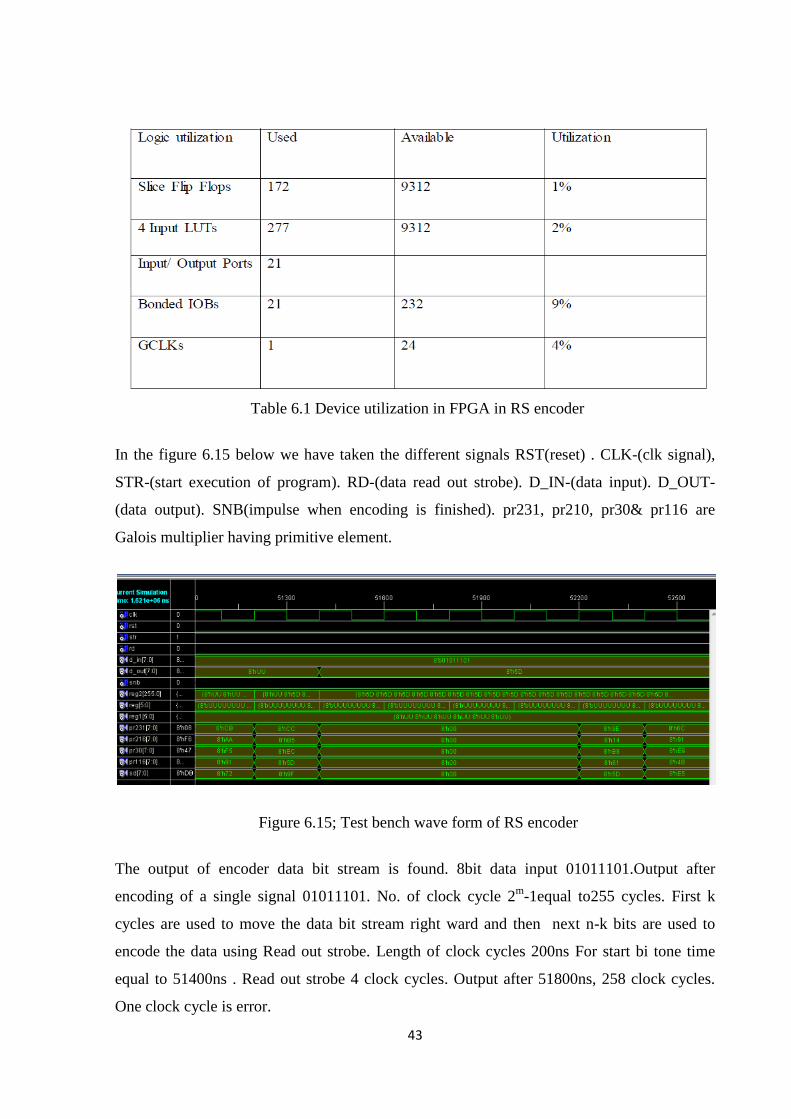
Table 6.1: Represents the Device utilization in FPGA in RS encoder 43
1
CHAPTER- 1
INTRODUCTION
Digital communication system is used to transport an information bearing signal from
the source to a user destination via a communication channel. A code is the set of all the
encoded words, the code word that an encoder can produce. When actual set of data encoded
it becomes a code.
Reed-Solomon error correcting codes (RS codes) are widely used in communication
systems and data storages to recover data from possible errors that occur during transmission
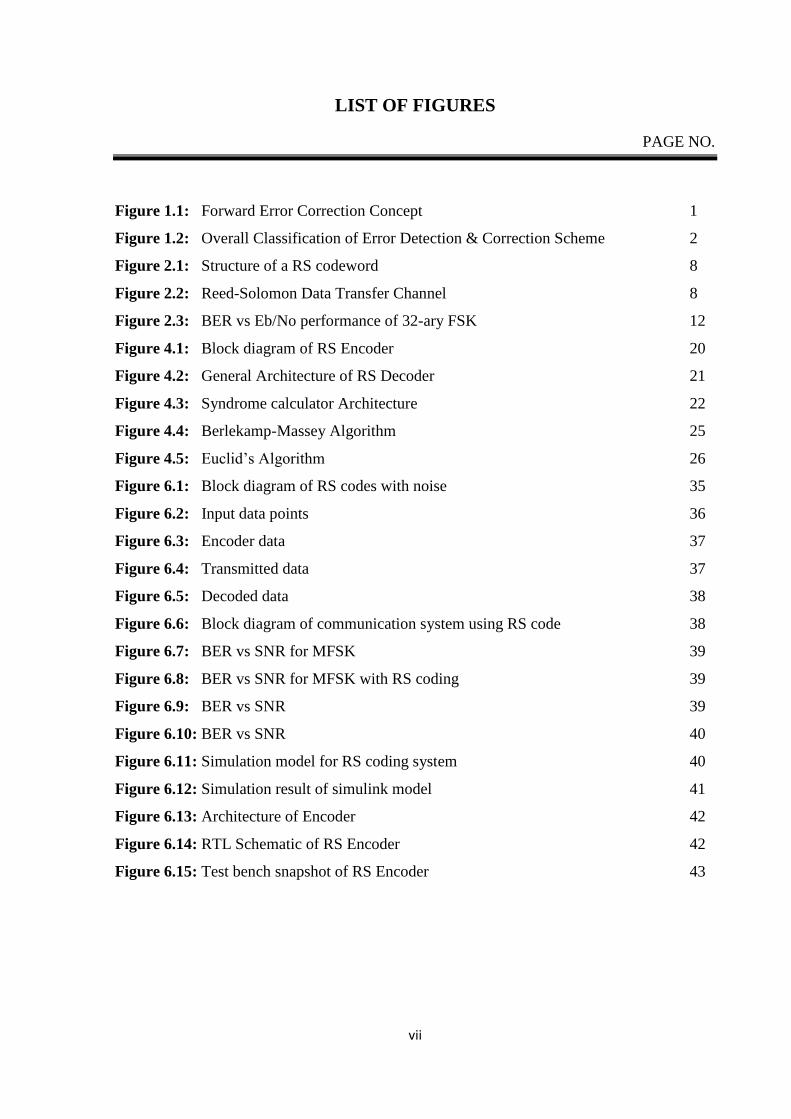
and from disc error respectively. One typical application of the RS codes is the Forward Error
Correction (FEC), the scheme is presented in Figure 1.1.
Figure 1.1: Forward Error Correction concept
Before data transmission, the encoder attaches parity symbols to the data using a
predetermined algorithm before transmission. At the receiving side, the decoder detects and
corrects a limited predetermined number of errors occurred during transmission. Transmitting
the extra parity symbols requires extra bandwidth compared to transmitting the pure data.
However, transmitting additional symbols introduced by FEC is better than retransmitting the
whole package when at least an error has been detected by the receiver [1] [2].
1.1 Error Detection & Correction Schemes
Error detection and correction or error controls are techniques that enable reliable
delivery of digital data over unreliable communication channel [3]. Many communication
channels are subject to channel noise, and thus errors may be introduced during transmission
from the source to a receiver. Error detection techniques allow detecting such errors, while
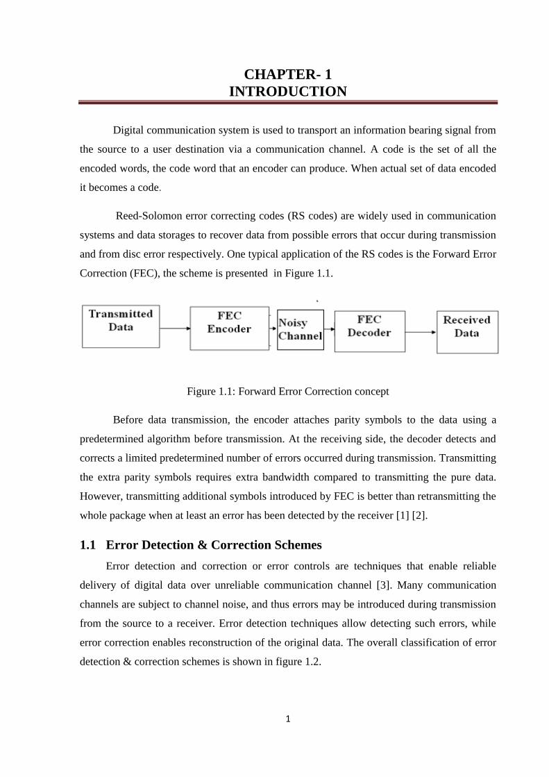
error correction enables reconstruction of the original data. The overall classification of error
detection & correction schemes is shown in figure 1.2.
2
Figure 1.2: Overall classification of error detection & correction schemes [1]
Different errors correcting codes can be used depending on the properties of the system
and the application in which the error correcting is to be introduced. Generally error –
correcting codes have been classified into block codes and convolutional codes. The
distinguishing feature for the classification is the presence or absence of memory in the
encoders for the two codes.
To generate a block code, the incoming information stream is divided into blocks and
each block is processed individually by adding redundancy in accordance with a prescribed
algorithm. The decoder processes each block individually and corrects errors by exploiting
redundancy.
In a convolutional code, the encoding operation may be viewed as the discrete–time
convolution of the input sequence with the impulse response of the encoder. The duration of
the impulse response equals the memory of the encoder. Accordingly, the encoder for a
convolutional code operates on the incoming message sequence, using a ―sliding window‖
equal in duration to its own memory. Hence in a convolutional code, unlike a block code
3
where code words are produced on a block─ by ─ block basis, the channel encoder accepts
message bits as continuous sequence and thereby generates a continuous sequence of encoded
bits at a higher rate [4].
An error-correcting code (ECC) or forward error correction (FEC) code is a system of
adding redundant data, or parity data, to a message, such that it can be recovered by a
receiver even when a number of errors (up to the capability of the code being used) were
introduced, either during the process of transmission, or on storage. Since the receiver does
not have to ask the sender for retransmission of the data, a back-channel is not required in
forward error correction, and it is therefore suitable for simplex communication such as
broadcasting. Error-correcting codes are frequently used in lower-layer communication, as
well as for reliable storage in media such as CDs, DVDs, hard disks, and RAM.
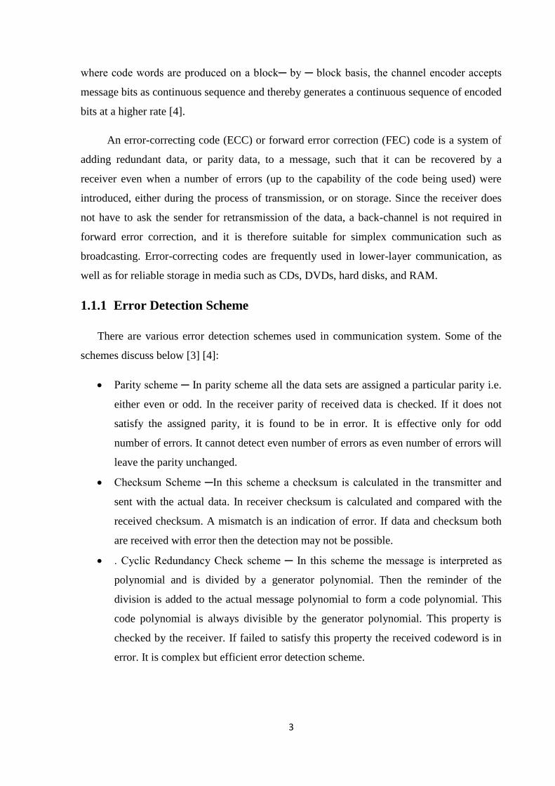
1.1.1 Error Detection Scheme
There are various error detection schemes used in communication system. Some of the
schemes discuss below [3] [4]:
Parity scheme ─ In parity scheme all the data sets are assigned a particular parity i.e.
either even or odd. In the receiver parity of received data is checked. If it does not
satisfy the assigned parity, it is found to be in error. It is effective only for odd
number of errors. It cannot detect even number of errors as even number of errors will
leave the parity unchanged.
Checksum Scheme ─In this scheme a checksum is calculated in the transmitter and
sent with the actual data. In receiver checksum is calculated and compared with the
received checksum. A mismatch is an indication of error. If data and checksum both
are received with error then the detection may not be possible.
. Cyclic Redundancy Check scheme ─ In this scheme the message is interpreted as
polynomial and is divided by a generator polynomial. Then the reminder of the
division is added to the actual message polynomial to form a code polynomial. This
code polynomial is always divisible by the generator polynomial. This property is
checked by the receiver. If failed to satisfy this property the received codeword is in
error. It is complex but efficient error detection scheme.
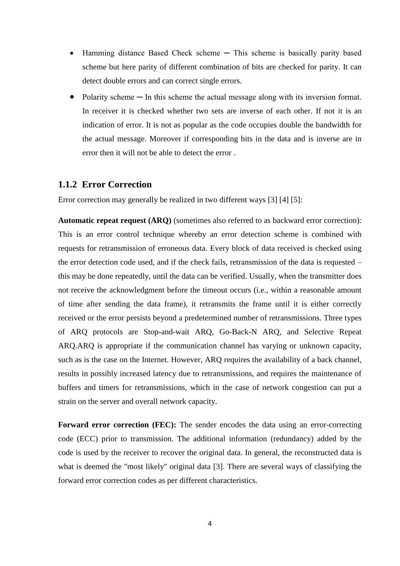
4
Hamming distance Based Check scheme ─ This scheme is basically parity based
scheme but here parity of different combination of bits are checked for parity. It can
detect double errors and can correct single errors.
Polarity scheme ─ In this scheme the actual message along with its inversion format.
In receiver it is checked whether two sets are inverse of each other. If not it is an
indication of error. It is not as popular as the code occupies double the bandwidth for
the actual message. Moreover if corresponding bits in the data and is inverse are in
error then it will not be able to detect the error .
1.1.2 Error Correction
Error correction may generally be realized in two different ways [3] [4] [5]:
Automatic repeat request (ARQ) (sometimes also referred to as backward error correction):
This is an error control technique whereby an error detection scheme is combined with
requests for retransmission of erroneous data. Every block of data received is checked using
the error detection code used, and if the check fails, retransmission of the data is requested –
this may be done repeatedly, until the data can be verified. Usually, when the transmitter does
not receive the acknowledgment before the timeout occurs (i.e., within a reasonable amount
of time after sending the data frame), it retransmits the frame until it is either correctly
received or the error persists beyond a predetermined number of retransmissions. Three types
of ARQ protocols are Stop-and-wait ARQ, Go-Back-N ARQ, and Selective Repeat
ARQ.ARQ is appropriate if the communication channel has varying or unknown capacity,
such as is the case on the Internet. However, ARQ requires the availability of a back channel,
results in possibly increased latency due to retransmissions, and requires the maintenance of
buffers and timers for retransmissions, which in the case of network congestion can put a
strain on the server and overall network capacity.
Forward error correction (FEC): The sender encodes the data using an error-correcting
code (ECC) prior to transmission. The additional information (redundancy) added by the
code is used by the receiver to recover the original data. In general, the reconstructed data is
what is deemed the "most likely" original data [3]. There are several ways of classifying the
forward error correction codes as per different characteristics.
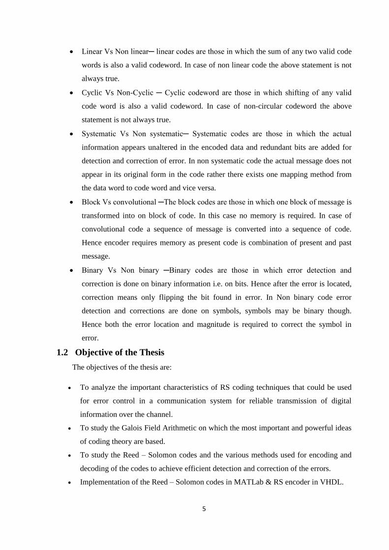
5
Linear Vs Non linear─ linear codes are those in which the sum of any two valid code
words is also a valid codeword. In case of non linear code the above statement is not
always true.
Cyclic Vs Non-Cyclic ─ Cyclic codeword are those in which shifting of any valid
code word is also a valid codeword. In case of non-circular codeword the above
statement is not always true.
Systematic Vs Non systematic─ Systematic codes are those in which the actual
information appears unaltered in the encoded data and redundant bits are added for
detection and correction of error. In non systematic code the actual message does not
appear in its original form in the code rather there exists one mapping method from
the data word to code word and vice versa.
Block Vs convolutional ─The block codes are those in which one block of message is
transformed into on block of code. In this case no memory is required. In case of
convolutional code a sequence of message is converted into a sequence of code.
Hence encoder requires memory as present code is combination of present and past
message.
Binary Vs Non binary ─Binary codes are those in which error detection and
correction is done on binary information i.e. on bits. Hence after the error is located,
correction means only flipping the bit found in error. In Non binary code error
detection and corrections are done on symbols, symbols may be binary though.
Hence both the error location and magnitude is required to correct the symbol in
error.
1.2 Objective of the Thesis
The objectives of the thesis are:
To analyze the important characteristics of RS coding techniques that could be used
for error control in a communication system for reliable transmission of digital
information over the channel.
To study the Galois Field Arithmetic on which the most important and powerful ideas
of coding theory are based.
To study the Reed – Solomon codes and the various methods used for encoding and
decoding of the codes to achieve efficient detection and correction of the errors.
Implementation of the Reed – Solomon codes in MATLab & RS encoder in VHDL.
6
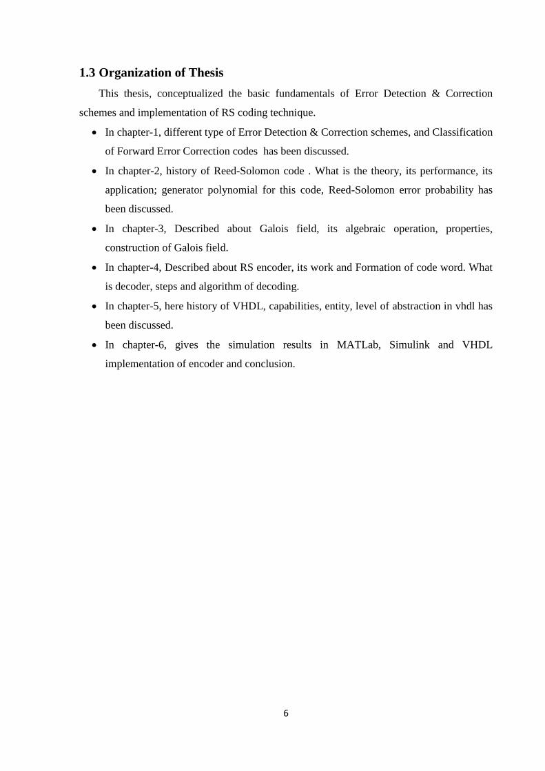
1.3 Organization of Thesis
This thesis, conceptualized the basic fundamentals of Error Detection & Correction
schemes and implementation of RS coding technique.
In chapter-1, different type of Error Detection & Correction schemes, and Classification
of Forward Error Correction codes has been discussed.
In chapter-2, history of Reed-Solomon code . What is the theory, its performance, its
application; generator polynomial for this code, Reed-Solomon error probability has
been discussed.
In chapter-3, Described about Galois field, its algebraic operation, properties,
construction of Galois field.
In chapter-4, Described about RS encoder, its work and Formation of code word. What
is decoder, steps and algorithm of decoding.
In chapter-5, here history of VHDL, capabilities, entity, level of abstraction in vhdl has
been discussed.
In chapter-6, gives the simulation results in MATLab, Simulink and VHDL
implementation of encoder and conclusion.
7
CHAPTER- 2
REED-SOLOMON CODE
Reed Solomon code is a linear cyclic systematic non-binary block code. In the
encoder Redundant symbols are generated using a generator polynomial and appended to the
message symbols. In decoder error location and magnitude are calculated using the same
generator polynomial. Then the correction is applied on the received code.
2.1 History
On January 21, 1959, Irving Reed and Gus Solomon submitted a paper to the Journal
of Society for Industrial and Applied Mathematics. In June of 1960 the paper was published:
―Polynomial Code over Certain Finite Fields‖. This paper described a new class of error–
correcting codes that are now called Reed-Solomon codes. Reed-Solomon codes have
enjoyed counterless applications, from compact disc players in living rooms all over the
planet to spacecraft that are now well beyond the orbit of Pluto. Reed-Solomon codes have
been an integral part of the telecommunications revolution in the last half of the twentieth
century. The first application, in 1982, of RS codes in mass-produced products was the
compact disc, where two interleaved RS codes are used. The key idea behind a Reed-
Solomon code is that the data encoded is first visualized as a polynomial. The code relies on a
theorem from algebra that states that any k distinct points uniquely determine a polynomial of
degree, at most, k - 1. The sender determines a degree k -1 polynomial, over a finite field that
represents the k data points. The polynomial is then encoded by its evaluation at various
points, and these values are what is actually sent. During transmission, some of these values
may become corrupted. Therefore, more than k points are actually sent. As long as sufficient
values are received correctly, the receiver can deduce what the original polynomial was, and
hence decode the original data. In the same sense that one can correct a curve by interpolating
past a gap, a Reed Solomon code can bridge a series of errors in a block of data to recover the
coefficients of the polynomial that drew the original curve [6][7].
2.2 Reed-Solomon Theory
A Reed-Solomon code is a block code and can be specified as RS (n,k) as shown in
Figure 2.1. The variable ‗n‘ is the size of the codeword with the unit of symbols, ‗k‘ is the
8
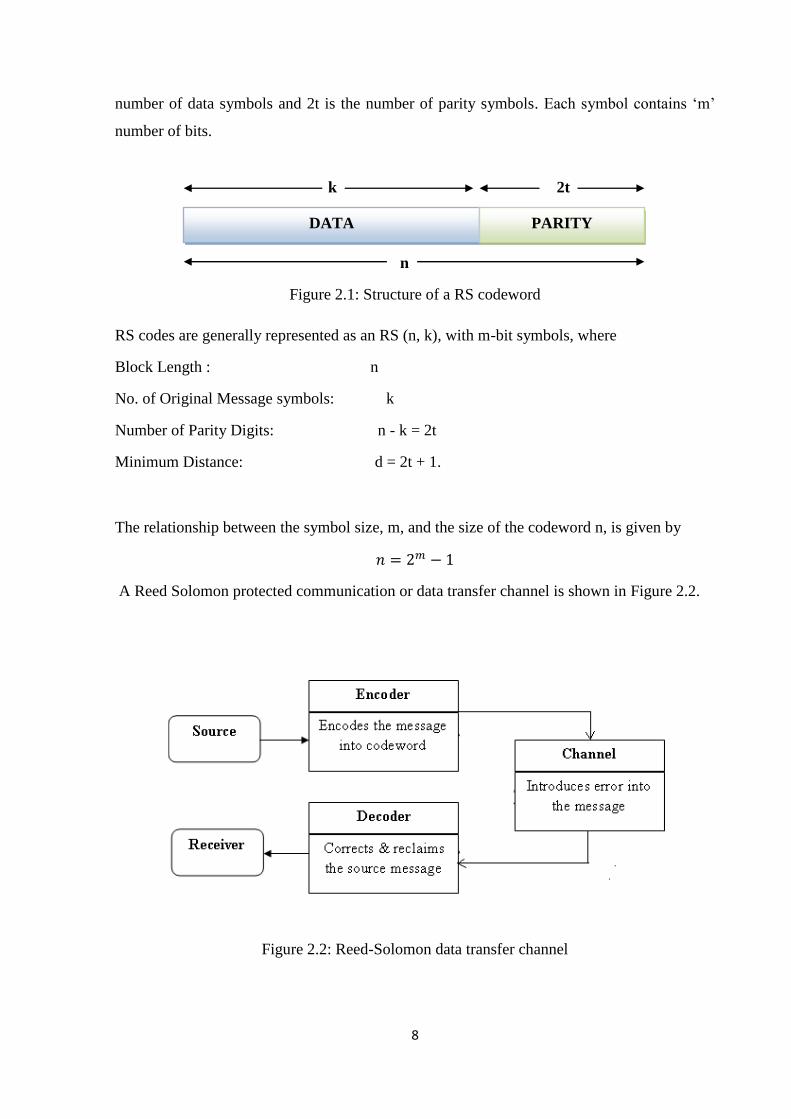
number of data symbols and 2t is the number of parity symbols. Each symbol contains ‗m‘
number of bits.
Figure 2.1: Structure of a RS codeword
RS codes are generally represented as an RS (n, k), with m-bit symbols, where
Block Length : n
No. of Original Message symbols: k
Number of Parity Digits: n - k = 2t
Minimum Distance: d = 2t + 1.
The relationship between the symbol size, m, and the size of the codeword n, is given by
A Reed Solomon protected communication or data transfer channel is shown in Figure 2.2.
Figure 2.2: Reed-Solomon data transfer channel
DATA PARITY
n
k 2t
9
The RS encoder provided at the transmitter end encodes the input message into a
codeword and transmits the same through the channel. Noise and other disturbances in the
channel may disrupt and corrupt the codeword. This corrupted codeword arrives at the
receiver end (decoder), where it gets checked and corrected message is passed on to the
receiver. In case the channel induced error is greater than the error correcting capability of the
decoder a decode failure can occur. Decoding failures are said to have occurred if a codeword
is passed unchanged, a decoding failure, on the other hand will lead to a wrong message
being given at the output [1].
2.2.1 Properties of Reed-Solomon Code
The topic of error correcting code is extensive and most texts treat all codes equally whether
they are easily implemented or not. Reed-Solomon code have certain properties which make
them useful in the real world.
RS codes are systematic linear block code. It‘s a block code because the code is put
together by splitting the original message in to a fixed length blocks. Each block is
further sub divided into m-bit symbols. Each symbol is fixed width, usually 3 to 8 bits
wide.
The linear nature of codes ensures that in practice every possible m-bit word is a valid
symbol. For instant with an 8-bit code all possible 8-bit words are valid for encoding,
Systematic means that the encoded data consists of original data with the extra parity
symbol appended to it.
The power of Reed-Solomon codes lies in being able to just as easily correct a corrupted
symbol with a single bit error as it can a symbol with all its bits in error. This makes RS
codes particularly suitable for correcting burst errors [8].
2.3 RS Code Performance
In error correction code for channel coding, the most common measure of performance is
the estimated probability of its decoder or transmission error. Since RS codes is a block codes
family that act on symbols level, its performance can be evaluated from different perspective
or functionality. As a function of size, if the block size increase, the error correcting codes
will be become more efficient or improve error performance. This is because, for a code to
10
successfully combat the effects or noise or channel impairments, the noise duration itself has
to be relatively small percentage of the whole codeword. For this to happen most of the time,
the received noise should be averaged out over a long period of time that will apparently
reduce the effect of the noise.
As a function of redundancy, as RS codes redundancy increases meaning at low code
rate, their implementations will grows in complexity and the bandwidth expansion must also
grow for any real time communication application. On the other hand, the profit of increased
in redundancy is just as the same when the size increase. That is the improvement in bit error
performance.
Lastly, as the function of code rate, as low code rate, the system will experienced
error performance degradation because the noise effect is very high. This is because the
information or message carries in the transmission is relatively small when compared to the
codeword that being transmitted even when only few error occurred. But on the other hand, at
optimum code rate where it approaches unity (as if there is no coding at all) the system will
suffer worse error performance since the error occurred couldn‘t be corrected or the corrected
capability is very limited for it to overcome the noise [9].
2.4 Application
Reed Solomon codes are error correcting codes that have found wide ranging applications
throughout the fields of digital communication and storage. Some of which include [10]:
Storage Devices (hard disks, compact disks, DVD, barcodes)
Wireless Communication (mobile phones, microwave links)
Digital Television
Broadband Modems (ADSL, xDSL, etc).
Deep Space and Satellite Communications Networks (CCSDS).
2.5 Generator Polynomial for a Reed-Solomon Code
A Reed Solomon code is a special case of a BCH code in which the length of the code is
one less than the size of the field over which the symbols are defined. It consists of sequences
of length (q – 1) whose roots include 2t consecutive powers of the primitive element of
GF(q). Alternatively, the Fourier transform over GF(q) will contain 2t consecutive zeros.
11
Note that because both the roots and the symbols are specified in GF(q), the generator
polynomial will have only the specified roots; there will be no Conjugates. Similarly the
Fourier transform of the generator sequence will be zero in only the specified 2t consecutive
positions.
A consequence of there being only 2t roots of the generator polynomial is that there are
only 2t parity checks. This is the lowest possible value for any t-error correcting code and is
known as the Singleton bound. To construct the generator for a Reed Solomon code, we need
only to construct the appropriate finite field and choose the roots. Suppose we decide that the
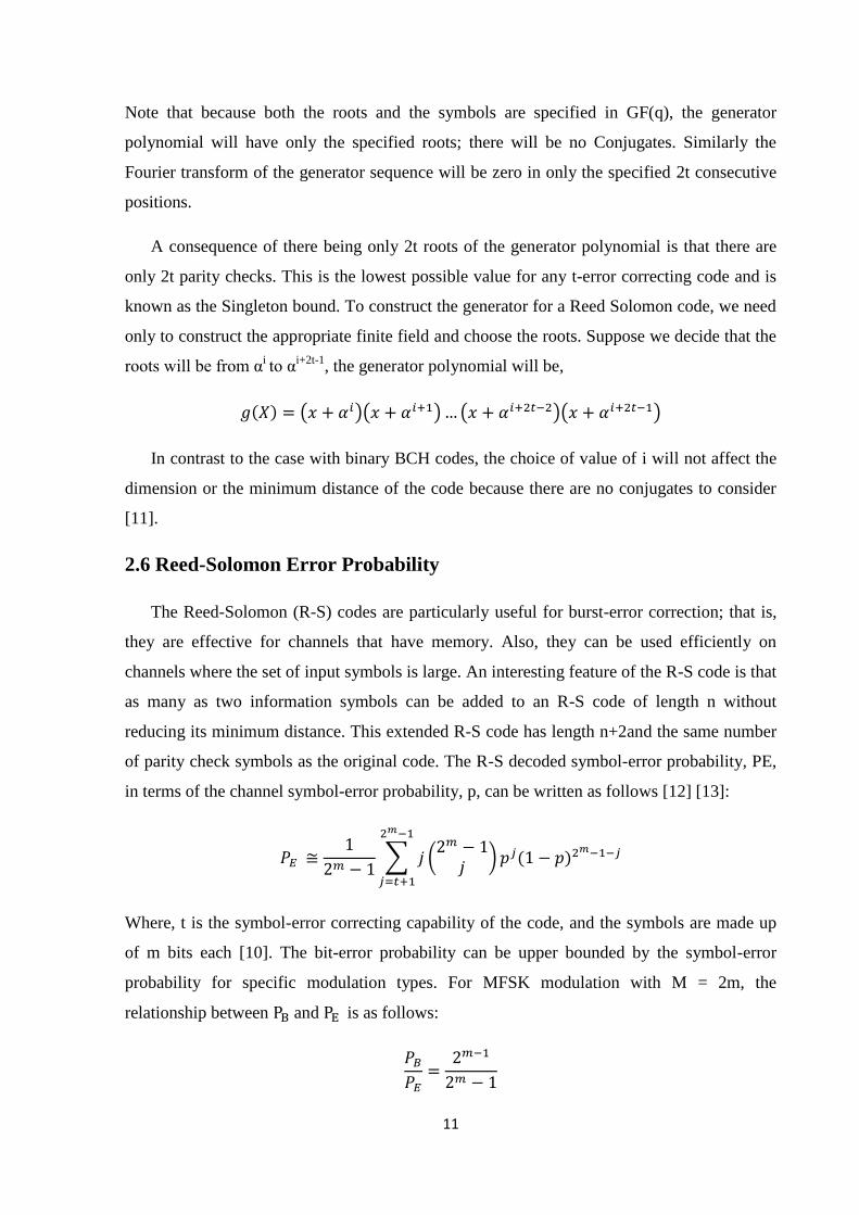
roots will be from αi to α
i+2t-1, the generator polynomial will be,
In contrast to the case with binary BCH codes, the choice of value of i will not affect the
dimension or the minimum distance of the code because there are no conjugates to consider
[11].
2.6 Reed-Solomon Error Probability
The Reed-Solomon (R-S) codes are particularly useful for burst-error correction; that is,
they are effective for channels that have memory. Also, they can be used efficiently on
channels where the set of input symbols is large. An interesting feature of the R-S code is that
as many as two information symbols can be added to an R-S code of length n without
reducing its minimum distance. This extended R-S code has length n+2and the same number
of parity check symbols as the original code. The R-S decoded symbol-error probability, PE,
in terms of the channel symbol-error probability, p, can be written as follows [12] [13]:
Where, t is the symbol-error correcting capability of the code, and the symbols are made up
of m bits each [10]. The bit-error probability can be upper bounded by the symbol-error
probability for specific modulation types. For MFSK modulation with M = 2m, the
relationship between and is as follows:
12
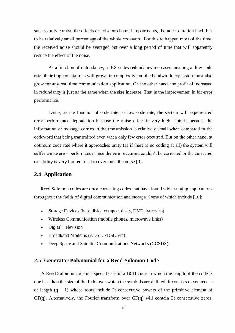
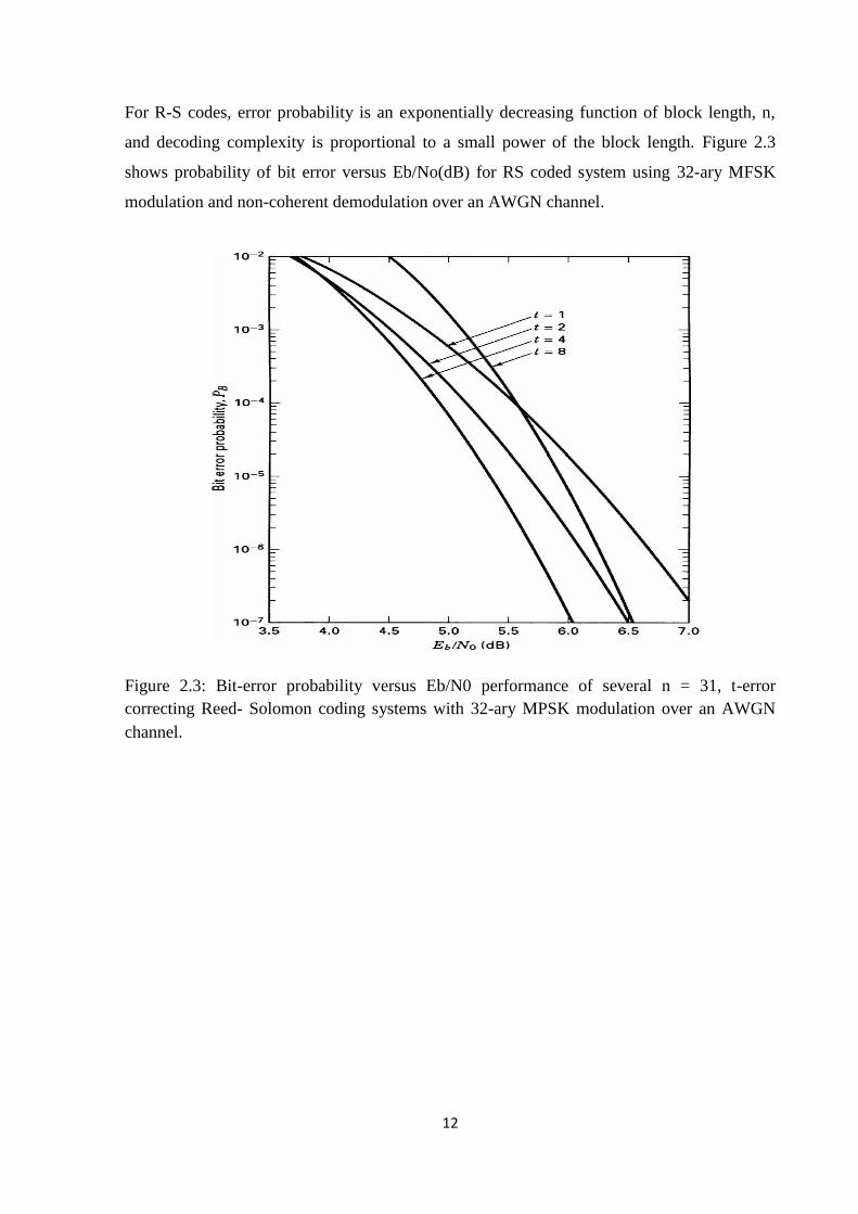
For R-S codes, error probability is an exponentially decreasing function of block length, n,
and decoding complexity is proportional to a small power of the block length. Figure 2.3
shows probability of bit error versus Eb/No(dB) for RS coded system using 32-ary MFSK
modulation and non-coherent demodulation over an AWGN channel.
Figure 2.3: Bit-error probability versus Eb/N0 performance of several n = 31, t-error
correcting Reed- Solomon coding systems with 32-ary MPSK modulation over an AWGN
channel.
13
CHAPTER- 3
GALOIS FIELD
The Reed-Solomon code is defined in the Galois field .which contains a finite set of numbers
where any arithmetic operations on elements of that set will result in an element belonging to
the same set.
3.1 Galois Field
In Galois field, every element, except zero, can be expressed as a power of a primitive
element, of the field. The non-zero field elements form a cyclic group defined based on a
binary primitive polynomial. An addition of two elements in the Galois field is simply the
exclusive-OR (XOR) operation [2]. However, a multiplication in the Galois field is more
complex than the standard arithmetic. It is the multiplication modulo the primitive
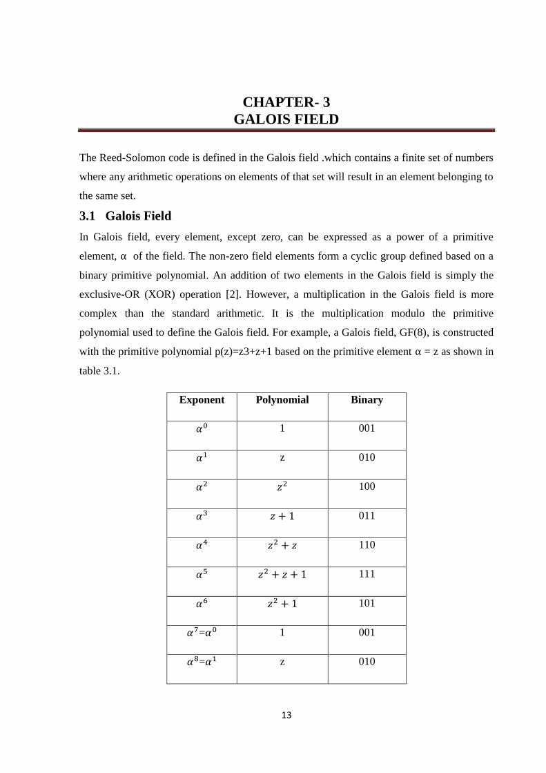
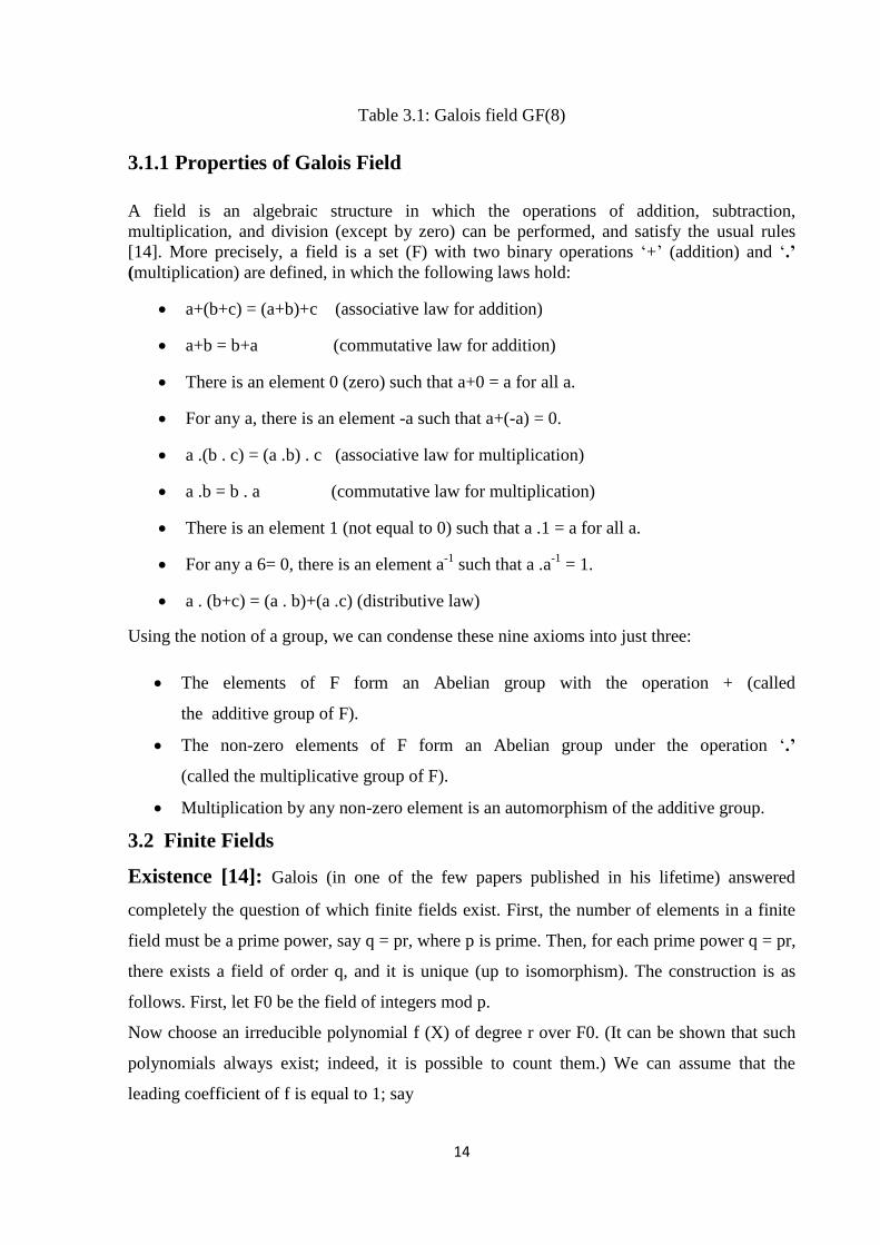
polynomial used to define the Galois field. For example, a Galois field, GF(8), is constructed
with the primitive polynomial p(z)=z3+z+1 based on the primitive element = z as shown in
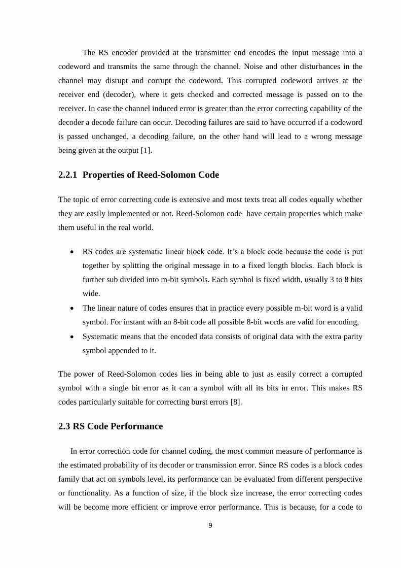
table 3.1.
Exponent Polynomial Binary
1 001
z 010
100
011
110
111
101
= 1 001
= z 010
14
Table 3.1: Galois field GF(8)
3.1.1 Properties of Galois Field
A field is an algebraic structure in which the operations of addition, subtraction,
multiplication, and division (except by zero) can be performed, and satisfy the usual rules
[14]. More precisely, a field is a set (F) with two binary operations ‗+‘ (addition) and ‗.’
(multiplication) are defined, in which the following laws hold:
a+(b+c) = (a+b)+c (associative law for addition)
a+b = b+a (commutative law for addition)
There is an element 0 (zero) such that a+0 = a for all a.
For any a, there is an element -a such that a+(-a) = 0.
a .(b . c) = (a .b) . c (associative law for multiplication)
a .b = b . a (commutative law for multiplication)
There is an element 1 (not equal to 0) such that a .1 = a for all a.
For any a 6= 0, there is an element a-1
such that a .a-1
= 1.
a . (b+c) = (a . b)+(a .c) (distributive law)
Using the notion of a group, we can condense these nine axioms into just three:
The elements of F form an Abelian group with the operation + (called
the additive group of F).
The non-zero elements of F form an Abelian group under the operation ‗.’
(called the multiplicative group of F).
Multiplication by any non-zero element is an automorphism of the additive group.
3.2 Finite Fields
Existence [14]: Galois (in one of the few papers published in his lifetime) answered
completely the question of which finite fields exist. First, the number of elements in a finite
field must be a prime power, say q = pr, where p is prime. Then, for each prime power q = pr,
there exists a field of order q, and it is unique (up to isomorphism). The construction is as
follows. First, let F0 be the field of integers mod p.
Now choose an irreducible polynomial f (X) of degree r over F0. (It can be shown that such
polynomials always exist; indeed, it is possible to count them.) We can assume that the
leading coefficient of f is equal to 1; say
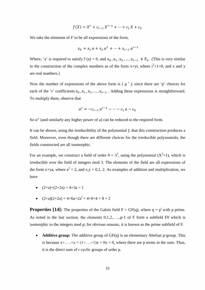
15
We take the elements of F to be all expressions of the form,
Where, ‗a‘ is required to satisfy f (a) = 0, and . (This is very similar
to the construction of the complex numbers as of the form x+yi, where i2+1=0, and x and y
are real numbers.)
Now the number of expressions of the above form is ( p r ), since there are ‗p‘ choices for
each of the ‗r‘ coefficients . Adding these expressions is straightforward.
To multiply them, observe that
So (and similarly any higher power of a) can be reduced to the required form.
It can be shown, using the irreducibility of the polynomial f, that this construction produces a
field. Moreover, even though there are different choices for the irreducible polynomials, the
fields constructed are all isomorphic.
For an example, we construct a field of order 9 = 32, using the polynomial (X
2+1), which is
irreducible over the field of integers mod 3. The elements of the field are all expressions of
the form x+ya, where a2 = 2, and x,y = 0,1, 2. As examples of addition and multiplication, we
have
(2+a)+(2+2a) = 4+3a = 1
(2+a)(2+2a) = 4+6a+2a2
= 4+0+4 = 8 = 2
Properties [14]: The properties of the Galois field F = GF(q), where q = pr with p prime.
As noted in the last section, the elements 0,1,2,…..,p-1 of F form a subfield F0 which is
isomorphic to the integers mod p; for obvious reasons, it is known as the prime subfield of F.
Additive group: The additive group of GF(q) is an elementary Abelian p-group. This
is because x+…..+x = (1+….+1)x = 0x = 0, where there are p terms in the sum. Thus,
it is the direct sum of r cyclic groups of order p.
16
Another way of saying this is that F is a vector space of dimension r over F1; that is, there is a
basis (a1,……,ar) such that every element x of F can be written uniquely in the form,
x = x1a1+…..+xrar
Multiplicative group: The most important result is that the multiplicative group of
GF(q) is cyclic; that is, there exists an element g called a primitive root) such that
every non-zero element of F can be written uniquely in the form gi for some i with 0≤
i ≤q-2. Moreover, we have gq-1
= g0 = 1.
3.3 Construction of Galois Fields
A Galois field GF (2 m
) with primitive element α is generally represented as (0, 1,α ,α2
,………. α2k-2
). The simplest example of a finite field is the binary field consisting of the
elements (0, 1). Traditionally referred to as GF(2) 2
, the operations in this field are defined as
integer addition and multiplication reduced modulo 2. Larger fields can be created by
extending GF(2) into vector space leading to finite fields of size 2 m
. These are simple
extensions of the base field GF(2) over m dimensions. The field GF(2 m
) is thus defined as a
field with 2 m
elements each of which is a binary m-tuple. Using this definition, m bits of
binary data can be grouped and referred to it as an element of GF(2 m
). This in turn allows
applying the associated mathematical operations of the field to encode and decode data [1]
[12][14].
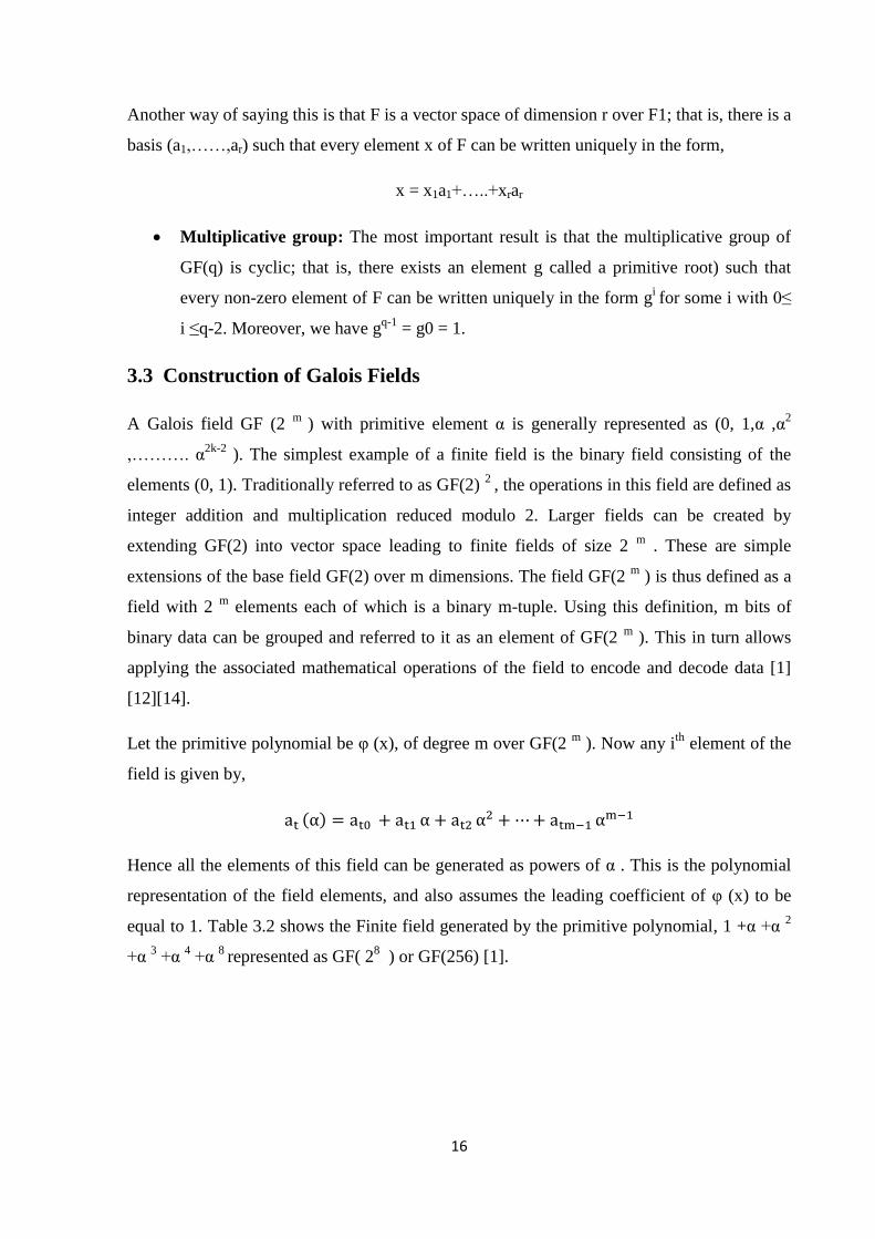
Let the primitive polynomial be φ (x), of degree m over GF(2 m
). Now any ith
element of the
field is given by,
Hence all the elements of this field can be generated as powers of α . This is the polynomial
representation of the field elements, and also assumes the leading coefficient of φ (x) to be
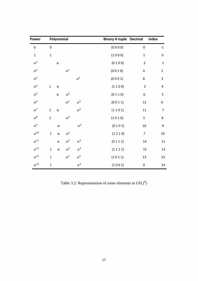
equal to 1. Table 3.2 shows the Finite field generated by the primitive polynomial, 1 +α +α 2
+α 3 +α
4 +α
8 represented as GF( 2
8 ) or GF(256) [1].
17
0 0 (0 0 0 0) 0 -1
1 1 (1 0 0 0) 1 0
α (0 1 0 0) 2 1
(0 0 1 0) 4 2
(0 0 0 1) 8 3
1 α (1 1 0 0) 3 4
α (0 1 1 0) 6 5
(0 0 1 1) 12 6
1 α (1 1 0 1) 11 7
1 (1 0 1 0) 5 8
α (0 1 0 1) 10 9
1 α (1 1 1 0) 7 10
α (0 1 1 1) 14 11
1 α (1 1 1 1) 15 12
1 (1 0 1 1) 13 13
1 (1 0 0 1) 9 14
Table 3.2: Representation of some elements in GF(28)
Power Polynomial Binary 4-tuple Decimal Index
18
CHAPTER- 4
REED-SOLOMON ENCODER & DECODER
4.1 RS Encoder
The Reed-Solomon encoder reads in k data symbols, computes the n - k parity symbols,
and appends the parity symbols to the k data symbols for a total of n symbols. The encoder is
essentially a 2t tap shift register where each register is m bits wide. The multiplier
coefficients are the coefficients of the RS generator polynomial. The general idea is the
construction of a polynomial; the coefficients produced will be symbols such that the
generator polynomial will exactly divide the data/parity polynomial [15].
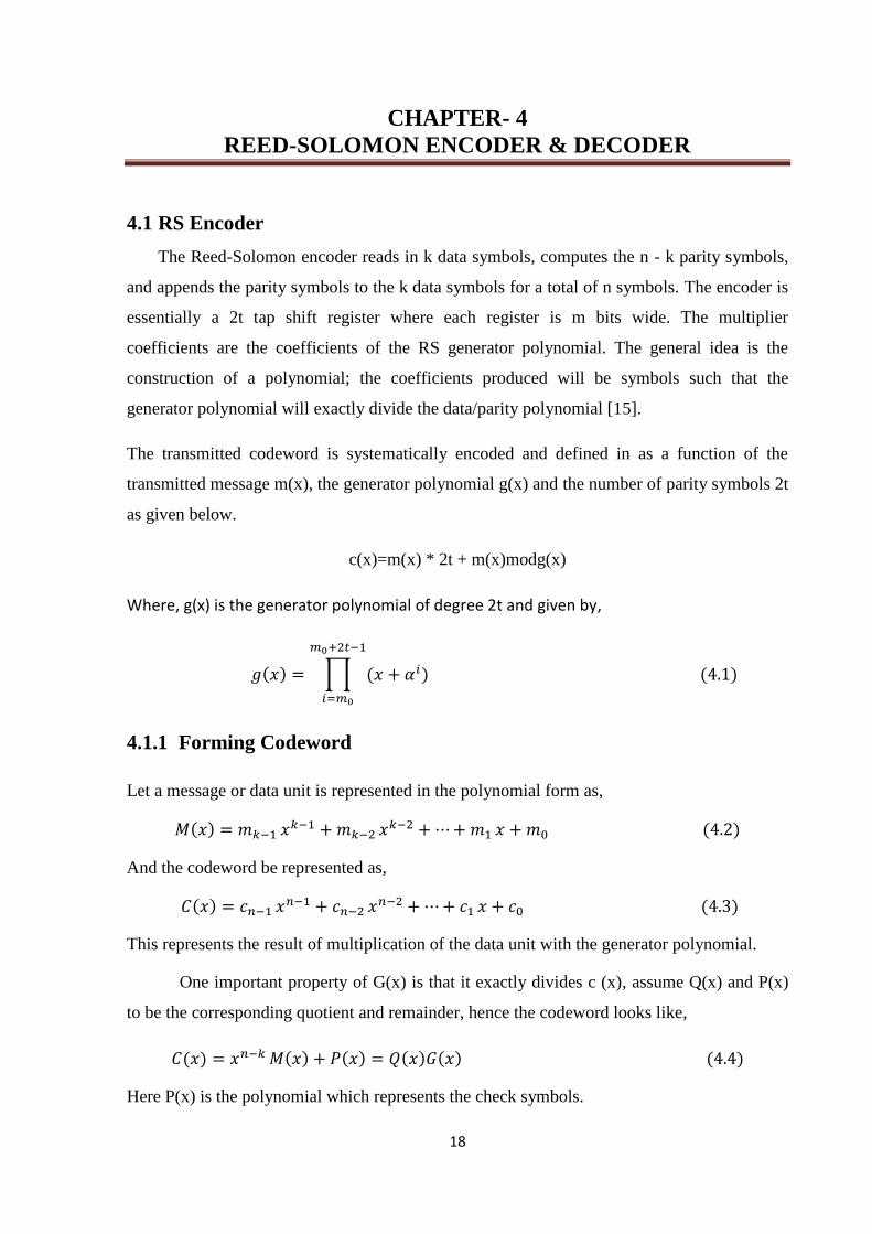
The transmitted codeword is systematically encoded and defined in as a function of the
transmitted message m(x), the generator polynomial g(x) and the number of parity symbols 2t
as given below.
c(x)=m(x) * 2t + m(x)modg(x)
Where, g(x) is the generator polynomial of degree 2t and given by,
4.1.1 Forming Codeword
Let a message or data unit is represented in the polynomial form as,
And the codeword be represented as,
This represents the result of multiplication of the data unit with the generator polynomial.
One important property of G(x) is that it exactly divides c (x), assume Q(x) and P(x)
to be the corresponding quotient and remainder, hence the codeword looks like,
Here P(x) is the polynomial which represents the check symbols.
19
Dividing by the generator polynomial and rewriting gives,
Here, Q(x) can be identified as ratio and – P(x) as a remainder after division by G(x). The
idea is that by concatenating these parity symbols to the end of data symbols, a codeword is
created which is exactly divisible by g(x). So when the decoder receives the message block, it
divides it with the RS generator polynomial. If the remainder is zero, then no errors are
detected, else indicates the presence of errors [1].
4.1.2 Operation
RS codes are systematic, so for encoding, the information symbols in the codeword
are placed as the higher power coefficients. This requires that information symbols must be
shifted from power level of (n-1) down to (n-k) and the remaining positions from power
(n-k-1) to 0 be filled with zeros. Therefore any RS encoder design should effectively perform
the following two operations, namely division and shifting. Both operations can be easily
implemented using Linear-Feedback Shift Registers [1][15][16].
Reed-Solomon codes may be shortened by (conceptually) making a number of data
symbols zero at the encoder, not transmitting them, and then re-inserting them at the decoder.
The encoder is essentially a 2t tap shift register where each register is m bits wide. The
multiplier coefficients are the coefficients of the RS generator polynomial. The general idea
is the construction of a polynomial; the coefficients produced will be symbols such that the
generator polynomial will exactly divide the data/parity polynomial. Encoder block diagram
is shown in figure 4.1.
20
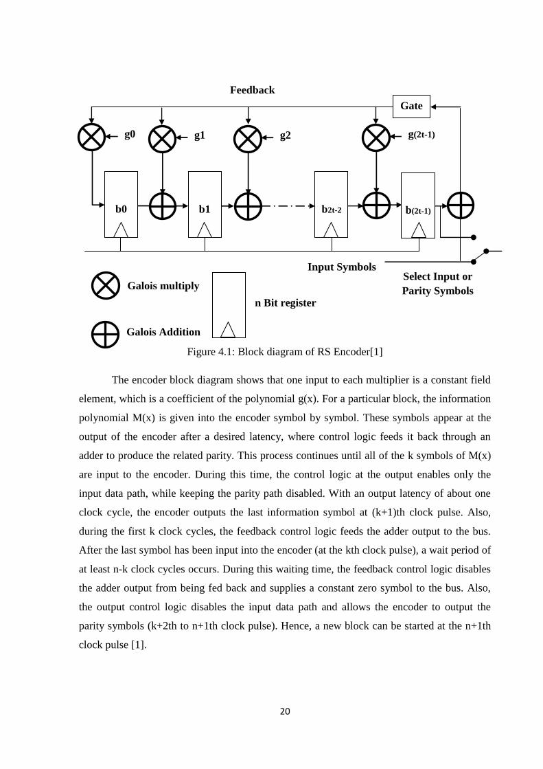
Figure 4.1: Block diagram of RS Encoder[1]
The encoder block diagram shows that one input to each multiplier is a constant field
element, which is a coefficient of the polynomial g(x). For a particular block, the information
polynomial M(x) is given into the encoder symbol by symbol. These symbols appear at the
output of the encoder after a desired latency, where control logic feeds it back through an
adder to produce the related parity. This process continues until all of the k symbols of M(x)
are input to the encoder. During this time, the control logic at the output enables only the
input data path, while keeping the parity path disabled. With an output latency of about one
clock cycle, the encoder outputs the last information symbol at (k+1)th clock pulse. Also,
during the first k clock cycles, the feedback control logic feeds the adder output to the bus.
After the last symbol has been input into the encoder (at the kth clock pulse), a wait period of
at least n-k clock cycles occurs. During this waiting time, the feedback control logic disables
the adder output from being fed back and supplies a constant zero symbol to the bus. Also,
the output control logic disables the input data path and allows the encoder to output the
parity symbols (k+2th to n+1th clock pulse). Hence, a new block can be started at the n+1th
clock pulse [1].
b1
g1
b0
g0 g2
b2t-2
g(2t-1)
b(2t-1)
Gate
Feedback
Input Symbols Select Input or
Parity Symbols n Bit register
Galois multiply
Galois Addition
21
4.2 RS Decoder
The Reed-Solomon decoder tries to correct errors and/or erasures by calculating the
syndromes for each codeword. Based upon the syndromes the decoder is able to determine
the number of errors in the received block [1][15][17]. If there are errors present, the decoder
tries to find the locations of the errors using the Berlekamp-Massey algorithm by creating an
error locator polynomial. The roots of this polynomial are found using the Chien search
algorithm. Using Forney's algorithm, the symbol error values are found and corrected. For an
RS (n, k) code where n - k = 2T, the decoder can correct up to T symbol errors in the code
word. Given that errors may only be corrected in units of single symbols (typically 8 data
bits), Reed-Solomon coders work best for correcting burst errors [11]. After going through a
noisy transmission channel, the encoded data can be represented as r(x) = c(x) + e(x), where
e(x) represents the error polynomial with the same degree as c(x) and r(x). Once the decoder
evaluates e(x), the transmitted message, c(x), is then recovered by adding the received
message, r(x), to the error polynomial, e(x), as given below:
c(x) = r(x) + e(x) = c(x) + e(x) + e(x) = c(x)
Note that e(x) + e(x) = 0 because addition in Galois field is equivalent to an exclusive-OR i.e
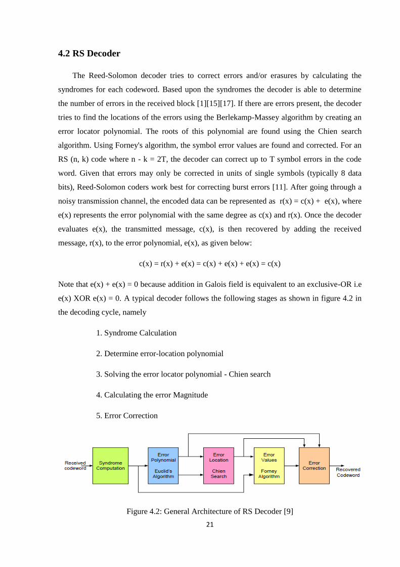
e(x) XOR e(x) = 0. A typical decoder follows the following stages as shown in figure 4.2 in
the decoding cycle, namely
1. Syndrome Calculation
2. Determine error-location polynomial
3. Solving the error locator polynomial - Chien search
4. Calculating the error Magnitude
5. Error Correction
Figure 4.2: General Architecture of RS Decoder [9]
22
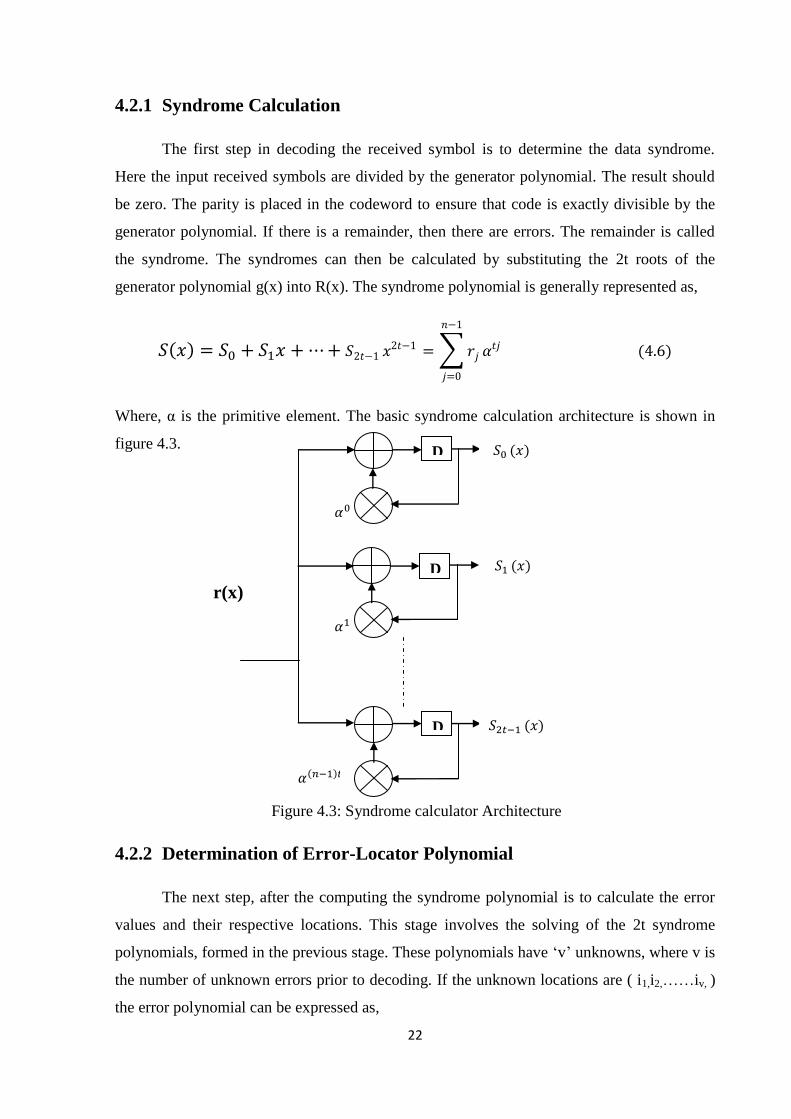
4.2.1 Syndrome Calculation
The first step in decoding the received symbol is to determine the data syndrome.
Here the input received symbols are divided by the generator polynomial. The result should
be zero. The parity is placed in the codeword to ensure that code is exactly divisible by the
generator polynomial. If there is a remainder, then there are errors. The remainder is called
the syndrome. The syndromes can then be calculated by substituting the 2t roots of the
generator polynomial g(x) into R(x). The syndrome polynomial is generally represented as,
Where, α is the primitive element. The basic syndrome calculation architecture is shown in
figure 4.3.
Figure 4.3: Syndrome calculator Architecture
4.2.2 Determination of Error-Locator Polynomial
The next step, after the computing the syndrome polynomial is to calculate the error
values and their respective locations. This stage involves the solving of the 2t syndrome
polynomials, formed in the previous stage. These polynomials have ‗v‘ unknowns, where v is
the number of unknown errors prior to decoding. If the unknown locations are ( i1,i2,……iv, )
the error polynomial can be expressed as,
D
D
D
r(x)
23
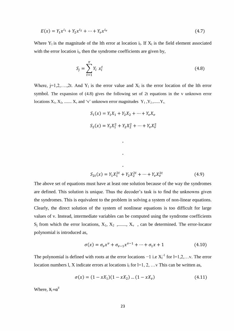
Where Yl is the magnitude of the lth error at location il. If Xl is the field element associated
with the error location il, then the syndrome coefficients are given by,
Where, j=1,2,….,2t. And Yl is the error value and Xl is the error location of the lth error
symbol. The expansion of (4.8) gives the following set of 2t equations in the v unknown error
locations X1, X2, ....... Xv and ‗v‘ unknown error magnitudes Y1 ,Y2 ,......Yv.
.
.
.
The above set of equations must have at least one solution because of the way the syndromes
are defined. This solution is unique. Thus the decoder‘s task is to find the unknowns given
the syndromes. This is equivalent to the problem in solving a system of non-linear equations.
Clearly, the direct solution of the system of nonlinear equations is too difficult for large
values of v. Instead, intermediate variables can be computed using the syndrome coefficients
Sj from which the error locations, X1, X2 ,......., Xv , can be determined. The error-locator
polynomial is introduced as,
The polynomial is defined with roots at the error locations −1 i.e Xl-1
for l=1,2,…v. The error
location numbers l, X indicate errors at locations il for l=1, 2, …v This can be written as,
Where, Xl =αil
24
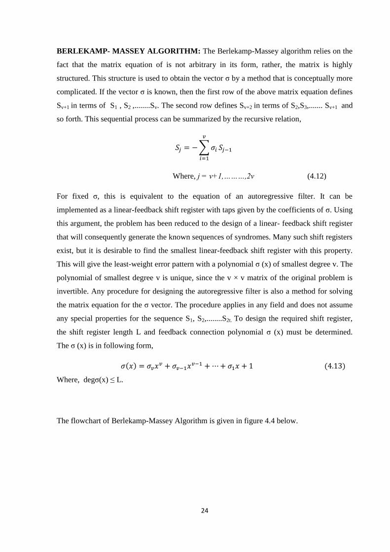
BERLEKAMP- MASSEY ALGORITHM: The Berlekamp-Massey algorithm relies on the
fact that the matrix equation of is not arbitrary in its form, rather, the matrix is highly
structured. This structure is used to obtain the vector σ by a method that is conceptually more
complicated. If the vector σ is known, then the first row of the above matrix equation defines
Sv+1 in terms of S1 , S2 ,........Sv. The second row defines Sv+2 in terms of S2,S3,....... Sv+1 and
so forth. This sequential process can be summarized by the recursive relation,
Where, j = v+1,………,2v (4.12)
For fixed σ, this is equivalent to the equation of an autoregressive filter. It can be
implemented as a linear-feedback shift register with taps given by the coefficients of σ. Using
this argument, the problem has been reduced to the design of a linear- feedback shift register
that will consequently generate the known sequences of syndromes. Many such shift registers
exist, but it is desirable to find the smallest linear-feedback shift register with this property.
This will give the least-weight error pattern with a polynomial σ (x) of smallest degree v. The
polynomial of smallest degree v is unique, since the v × v matrix of the original problem is
invertible. Any procedure for designing the autoregressive filter is also a method for solving
the matrix equation for the σ vector. The procedure applies in any field and does not assume
any special properties for the sequence S1, S2,........S2t. To design the required shift register,
the shift register length L and feedback connection polynomial σ (x) must be determined.
The σ (x) is in following form,
Where, degσ(x) ≤ L.
The flowchart of Berlekamp-Massey Algorithm is given in figure 4.4 below.
25
Figure 4.4: Berlekamp-Massey Algorithm [2]
Initialization
Compute error in next syndrome
Compute new correction polynomial for
which
Proceed to Next Step
Yes
No
Normalize and store old shift reg.
Update shift reg.
Update length
More than t errors
No
No
No
Yes
Yes
Yes
26
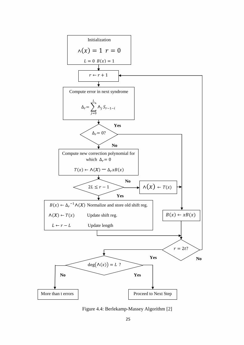
EUCLID'S ALGORITHM: Euclid's algorithm is a recursive procedure for calculating the
greatest common divisor (GCD) of two polynomials. In a slightly expanded version, the
algorithm will always produce the polynomials a(x) and b(x) satisfying,
GCD [s(x), t(x)] = a(x)s(x) + b(x)t(x)
The flowchart for Euclid‘s Algorithm Is given in figure 4.5 below.
Figure 4.5: Euclid‘s Algorithm [2]
Initialization
Compute the quotient
Compute
Proceed to Next Step
Yes
No
27
4.2.3 Solving the Error Locator Polynomial-CHIEN Search
Once the error locator and error evaluator polynomials have been determined using the
above techniques, the next step in the decoding process is to evaluate the error polynomial
and obtain its roots. The roots thus obtained will now point to the error locations in the
received message. RS decoding generally employs the Chien search scheme to implement the
same. A number ‘n‘ is said to be a root of a polynomial, if the result of substitution of its
value in the polynomial evaluates to zero. Chien Search is a brute force approach for guessing
the roots, and adopts direct substitution of elements in the Galois field, until a specific i from
i=0, 1,.., (n-1) is found such that σ (αi) = 0 . In such a case α
i is said to be the root and the
location of the error is evaluated as σ(x). Then the number of zeros of the error locator
polynomial σ(x) is computed and is compared with the degree of the polynomial. If a match
is found the error vector is updated and σ (x) is evaluated in all symbol positions of the
codeword. A mismatch indicates the presence of more errors than can be corrected [1].
4.2.4 Error Value Computation-FORNEY Algorithm
Once the errors are located, the next step is to use the syndromes and the error
polynomial roots to derive the error values. Forney Algorithm is generally used for this
purpose [1]. It is an efficient way of performing a matrix inversion, and involves two main
stages.
First the error evaluator polynomial ω(x) is calculated. This is done by convolving the
syndromes with the error polynomial σ(x) (from the Euclid‘s algorithm).
This calculation is carried out at each zero location, and the result thus arrived is then divided
by the derivative of lambda. Each such calculation gives the error symbol at the
corresponding location. The error magnitude at each error location is given by,
(4.15)
If the error symbol has any set bit, it means that the corresponding bit in the received symbol
is at error, and must be inverted. To automate this correction process each of the received
symbol is read again (from an intermediate store), and at each error location the received
28
symbols XOR‘ed with the error symbol. Thus the decoder corrects any errors as the received
word is being read out from it.
In summary, the decoding algorithm works as follows [1]:
Step 1: Calculate the syndromes according to Equation (4.6)
Step2: Perform the Berlekamp-Massey or Euclid's algorithm to obtain the error locator
polynomial σ (x). Also find the error evaluator polynomial ω(x).
Step 3: Perform the Chien Search to find the roots of σ (x).
Step 4: Find the magnitude of the error values using the Forney‘s Algorithm.
Step 5: Correct the received word C ( x ) = E(x) + R ( x )
29
CHAPTER- 5
VHSIC HARDWARE DESCRIPTION LANGUAGE
VHDL is an acronym for VHSIC Hardware Description Language(VHSIC is an
acronym for Very High Speed Integrated Circuits).It is a hardware description language that
can be used to model a digital system at many levels of abstraction, ranging from the
algorithmic level to the gate level[18].
Hardware description languages are especially useful to gain more control of parallel
processes as well as to circumvent some of the idiosyncrasies of the higher level
programming languages. The compilers often add latency to loops during compilation for
implementation. This can be difficult to fix in the higher-level languages, though the solution
may be quite obvious at the hardware description level. One particularly frustrating
peculiarity is the implementation of multipliers. For all multiply commands, the complier
requires three multipliers to be used, though typically one is sufficient. The compiler‘s
multipliers also are intended for integers. For a fixed-point design, the decimal point must be
moved after every multiply. This is much easier to implement at the hardware description
level [1].
VHDL is a programming language that has been designed and optimized for
describing the behavior of digital systems. VHDL has many features appropriate for
describing the behaviour of electronic components ranging from simple logic gates to
complete microprocessors and custom chips. Features of VHDL allow electrical aspects of
circuit behavior such as rise and fall times of signals, delays through gates, and functional
operation to be precisely described. The resulting VHDL simulation models can then be used
as building blocks in larger circuits using schematics, block diagrams or system-level VHDL
descriptions for the purpose of simulation.
VHDL is also a general-purpose programming language: just as high-level
programming languages allow complex design concepts to be expressed as computer
programs, VHDL allows the behavior of complex electronic circuits to be captured into a
design system for automatic circuit synthesis or for system simulation. Like Pascal, C and
C++, VHDL includes features useful for structured design techniques, and offers a rich set of
control and data representation features. Unlike these other programming languages, VHDL
provides features allowing concurrent events to be described. This is important because the
30
hardware described using VHDL is inherently concurrent in its operation. One of the most
important applications of VHDL is to capture the performance specification for a circuit, in
the form of what is commonly referred to as a test bench. Test benches are VHDL
descriptions of circuit stimuli and corresponding expected outputs that verify the behaviour of
a circuit over time. Test benches should be an integral part of any VHDL project and should
be created in tandem with other descriptions of the circuit. One of the most compelling
reasons for learning VHDL is its adoption as a standard in the electronic design community.
Using a standard language such as VHDL virtually guarantees that the engineers will not
have to throw away and recapture design concepts simply because the design entry method
chosen is not supported in a newer generation of design tools. Using a standard language also
means that the engineer is more likely to be able to take advantage of the most up-to-date
design tools and that the users of the language will have access to a knowledge base of
thousands of other engineers, many of whom are solving similar problems.
5.1 History of VHDL
1981 - Initiated by US DoD to address hardware life-cycle crisis
1983-85 - Development of baseline language by Intermetrics, IBM and TI
1986 - All rights transferred to IEEE
1987 - Publication of IEEE Standard
1987 - Mil Std 454 requires comprehensive VHDL descriptions to be delivered
with Asics
1994 - Revised standard (named VHDL 1076-1993)
31
5.2 Capabilities
The following are the major capabilities that the language provides along with the
features that differentiated from other hardware description language [18].
The language can be used as an exchange medium between chip vendors and CAD
tool users. Different chip vendors can provide VHDL description of their components
to system designers.
The language can also be used as communication medium between different CAD
and CAE tools.
The language supports hierarchy; that is a digital system can be modelled as a set of
interconnected components.
The language supports flexible design methodologies: top-down, bottom-up, or
mixed.
The language is not technology-specific, but is capable of supporting technology-
specific features. It can also support various hardware technologies.
It supports both synchronous and asynchronous timing models.
Various digital modelling techniques, such as finite-state machine descriptions,
algorithmic descriptions and Boolean equations, can be model using the language.
The language is publicly available, human-readable, machine-readable and above all,
it is not proprietary.
It is an IEEE and ANSI standard; therefore model described using this language is
portable.
The language supports three basic different description styles: structural, data flow
and behavioural. A design may also be expressed in any combination of these three.
It supports a wide range of abstraction levels ranging from abstract behavioural
descriptions to very precise gate-level descriptions.
Arbitrarily large designs can be modelled using this language, and there are no
limitations imposed by the language on the size of design.
The language has elements that make large-scale design modelling easier.
Nominal propagation delays, min-max delays, setup and hold timing, timing
constraints and spike detection can all be described very naturally in this language.
32
5.3 Design Units
Every VHDL design description consists of at least one entity/architecture pair.To
describe an entity, VHDL provides five different types of primary constructs, called design
units [1] [17][19]. They are:
Entity declaration
Architecture body
Configuration declaration
Package declaration
Package body
An entity is modelled using an entity declaration and at least one architecture body.
The entity declaration describes the external view of the entity; for example the input and
output signal names.
The configuration declaration is used to create a configuration for an entity. It
specifies the binding of one architecture body from many architecture bodies that may be
associated with the entity. An entity will have any number of different configurations.
A package declaration encapsulates a set of related declarations, such as type declaration,
sub type declarations, and subprogram declaration, which can be shared across two or more
design units .
5.4 Levels of Abstraction
VHDL supports many possible styles of design description. These styles differ primarily
in how closely they relate to the underlying hardware. When we speak of the different styles
of VHDL, we are really talking about the differing levels of abstraction possible using the
language—behavior, dataflow, and structure [1].
5.4.1 Behavior
The highest level of abstraction supported in VHDL is called the behavioral level of
abstraction. When creating a behavioral description of a circuit, the circuits is described in
terms of its operation over time. The concept of time is the critical distinction between
33
behavioral descriptions of circuits and lower-level descriptions specifically descriptions
created at the dataflow level of abstraction.
In a behavioral description, the concept of time can be expressed precisely, with actual
delays between related events (such as the propagation delays within gates and on wires), or
it may simply be an ordering of operations that are expressed sequentially (such as in a
functional description of a flip-flop). While writing VHDL for input to synthesis tools,
behavioural statements in VHDL can be used to imply that there are registers in your circuit.
It is unlikely, however, that the synthesis tool will be capable of creating precisely the same
behavior in actual circuitry as defined in the language. It is also unlikely that the synthesis
tool will be capable of accepting and processing a very wide range of behavioral description
styles [1].
5.4.2 Dataflow
In the dataflow level of abstraction, the circuit is described in terms of how data moves
through the system. Registers are the most important part of most digital systems today, so in
the dataflow level of abstraction it is described how the information is passed between
registers in the circuit. The combinational logic portion of the circuit may also be described at
a relatively high level (and let a synthesis tool figure out the detailed implementation in logic
gates), but specifications about the placement and operation of registers in the complete
circuit are given by the user. The dataflow level of abstraction is often called register transfer
logic, or RTL [1].
5.4.3 Structure
The third level of abstraction is structure. It is used to describe a circuit in terms of its
components. Structure can be used to create a very low-level description of a circuit such as a
transistor-level description or a very high-level description such as a block diagram. In a
gate-level description of a circuit, components such as basic logic gates and flip-flops might
be connected in some logical structure to create the circuit. This is often called a net list.
For a higher-level circuit — one in which the components being connected are larger
functional blocks — structure might simply be used to segment the design description into
manageable parts.
34
Structure-level VHDL features, such as components and configurations, are very useful
for managing complexity. The use of components can dramatically improve the ability to re-
use elements of the designs and they can make it possible to work using a top-down design
approach [1].
5.5 Objects
VHDL includes a number of language elements, collectively called objects that can be used
to represent and store data in the system being described. Three basic types of objects that are
used when entering a design description for synthesis or creating functional tests (in the form
of a test bench) are signals, variables and constants. Each object that is declared has a specific
data type (such as bit or integer) and a unique set of possible values.
5.5.1 Signals
Signals are objects that are used to connect concurrent elements (such as components,
processes and concurrent assignments), similar to the way that wires are used to connect
components on a circuit board or in a schematic. Signals can be declared globally in an
external package or locally within architecture, block or other declarative region.
5.5.2 Variables
Variables are objects used to store intermediate values between sequential VHDL
statements. Variables are only allowed in processes, procedures and functions, and they are
always local to those functions. The 1076-1993 language standard adds a new type of global
variable that has visibility between different processes and subprograms. Variables in VHDL
are much like variables in a conventional software programming language. They immediately
take on and store the value assigned to them and they can be used to simplify a complex
calculation or sequence of logical operations.
35
CHAPTER- 6
SIMULATION RESULTS OF REED-SOLOMON CODES IN
MATLAB & VHDL
In previous chapters RS codes and their encoding and decoding procedures were thoroughly
discussed and this chapter describes the implementation of RS codes in MATLAB and
VHDL and their simulation results.
6.1 Implementation of RS Code in MATLAB
Our main aim for simulating the RS code in MATLAB was to understand the phenomenon as
how the signal is being encoded and, what would happen if the signal has some error and up
to what extent, the decoder can detect and correct errors. In first simulation MATLAB, a
random symbol of integers was taken as input. These random symbols were then encoded
using RS encoder. Following this signal was passed through AWGN channel, these symbols
were then received at the decoder end. Now at the decoder end, the decoder can correct up to
t symbols.. The reed Solomon decoder actually corrects symbols up to 2t symbols from the n
number of symbols. It never matters whether the errors are in parity symbols or the
information symbols. After correcting the error, however the decoder takes the redundant bits
out which were generated while encoding the symbols.
6.1.1 RS Codes with Noise
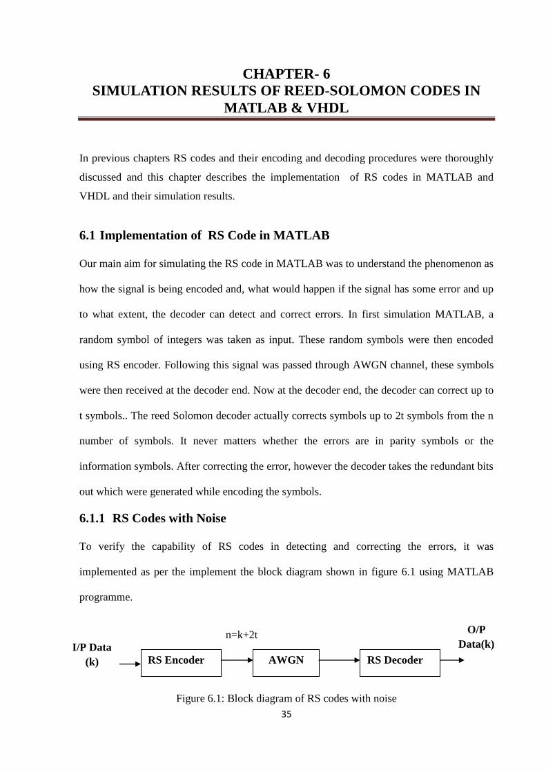
To verify the capability of RS codes in detecting and correcting the errors, it was
implemented as per the implement the block diagram shown in figure 6.1 using MATLAB
programme.
Figure 6.1: Block diagram of RS codes with noise
RS Encoder AWGN RS Decoder
I/P Data
(k)
O/P
Data(k)
) (k)
n=k+2t
36
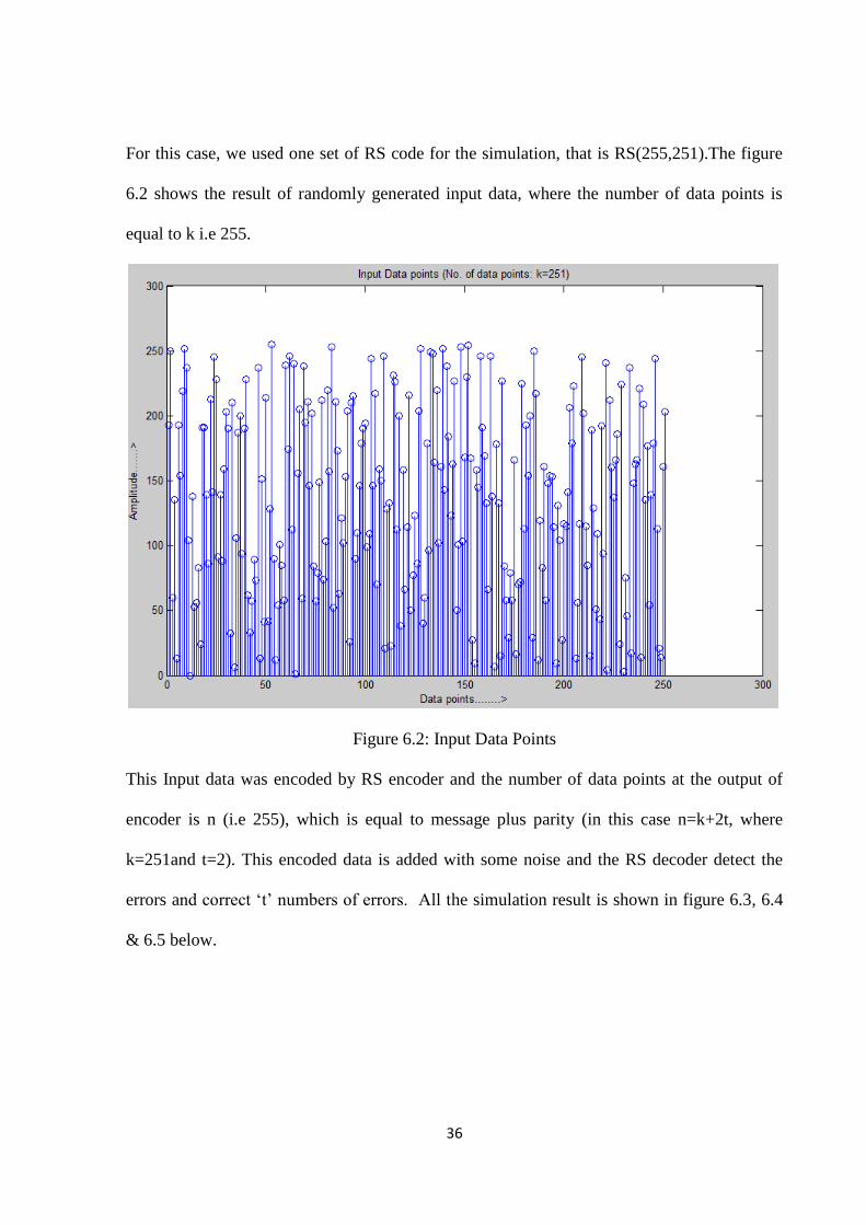
For this case, we used one set of RS code for the simulation, that is RS(255,251).The figure
6.2 shows the result of randomly generated input data, where the number of data points is
equal to k i.e 255.
Figure 6.2: Input Data Points
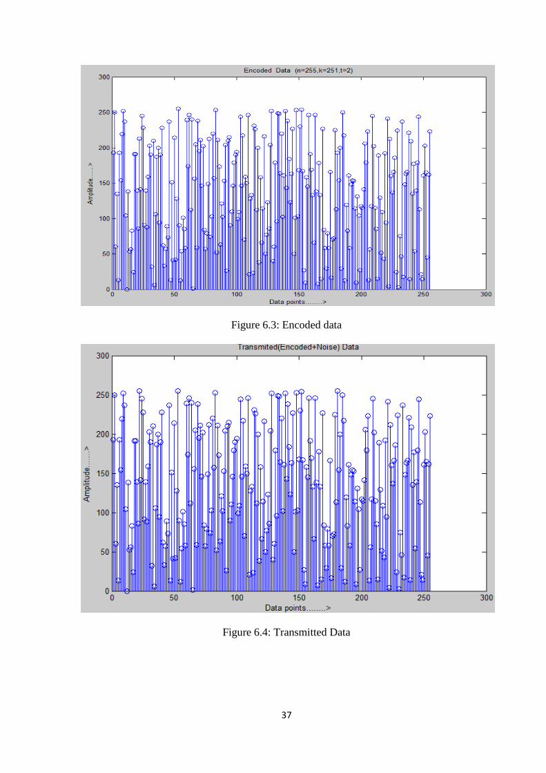
This Input data was encoded by RS encoder and the number of data points at the output of
encoder is n (i.e 255), which is equal to message plus parity (in this case n=k+2t, where
k=251and t=2). This encoded data is added with some noise and the RS decoder detect the
errors and correct ‗t‘ numbers of errors. All the simulation result is shown in figure 6.3, 6.4
& 6.5 below.
37
Figure 6.3: Encoded data
Figure 6.4: Transmitted Data
38
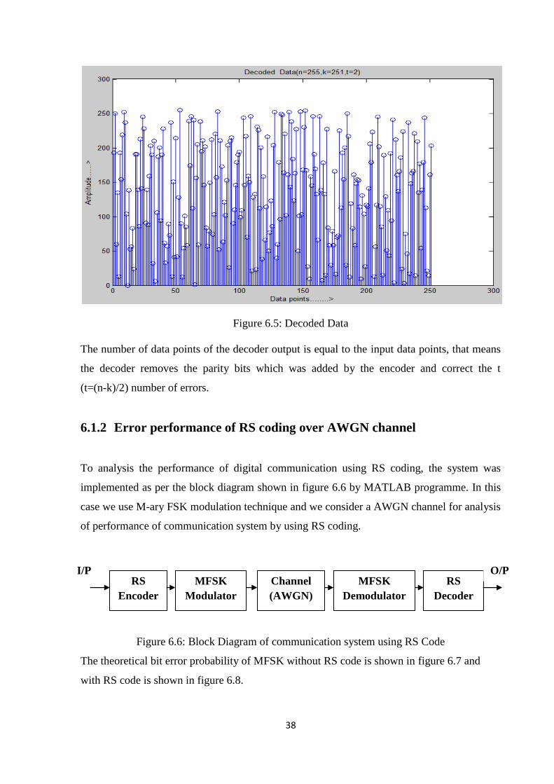
Figure 6.5: Decoded Data
The number of data points of the decoder output is equal to the input data points, that means
the decoder removes the parity bits which was added by the encoder and correct the t
(t=(n-k)/2) number of errors.
6.1.2 Error performance of RS coding over AWGN channel
To analysis the performance of digital communication using RS coding, the system was
implemented as per the block diagram shown in figure 6.6 by MATLAB programme. In this
case we use M-ary FSK modulation technique and we consider a AWGN channel for analysis
of performance of communication system by using RS coding.
Figure 6.6: Block Diagram of communication system using RS Code
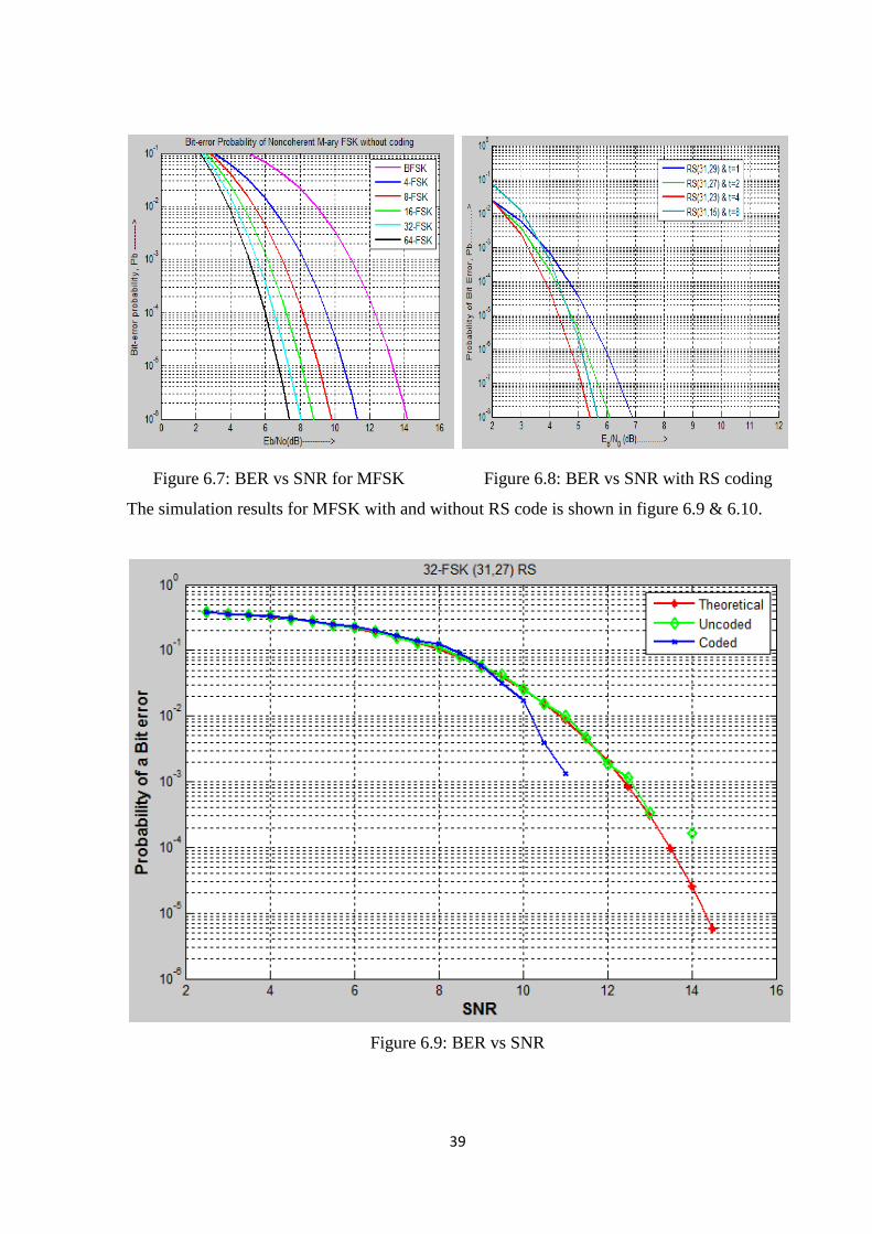
The theoretical bit error probability of MFSK without RS code is shown in figure 6.7 and
with RS code is shown in figure 6.8.
RS
Encoder
Channel
(AWGN)
MFSK
Modulator
MFSK
Demodulator
RS
Decoder
I/P O/P
39
Figure 6.7: BER vs SNR for MFSK Figure 6.8: BER vs SNR with RS coding
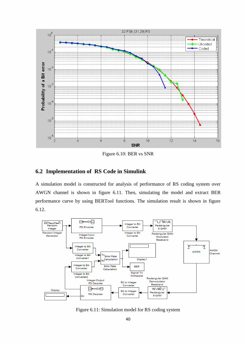
The simulation results for MFSK with and without RS code is shown in figure 6.9 & 6.10.
Figure 6.9: BER vs SNR
40
Figure 6.10: BER vs SNR
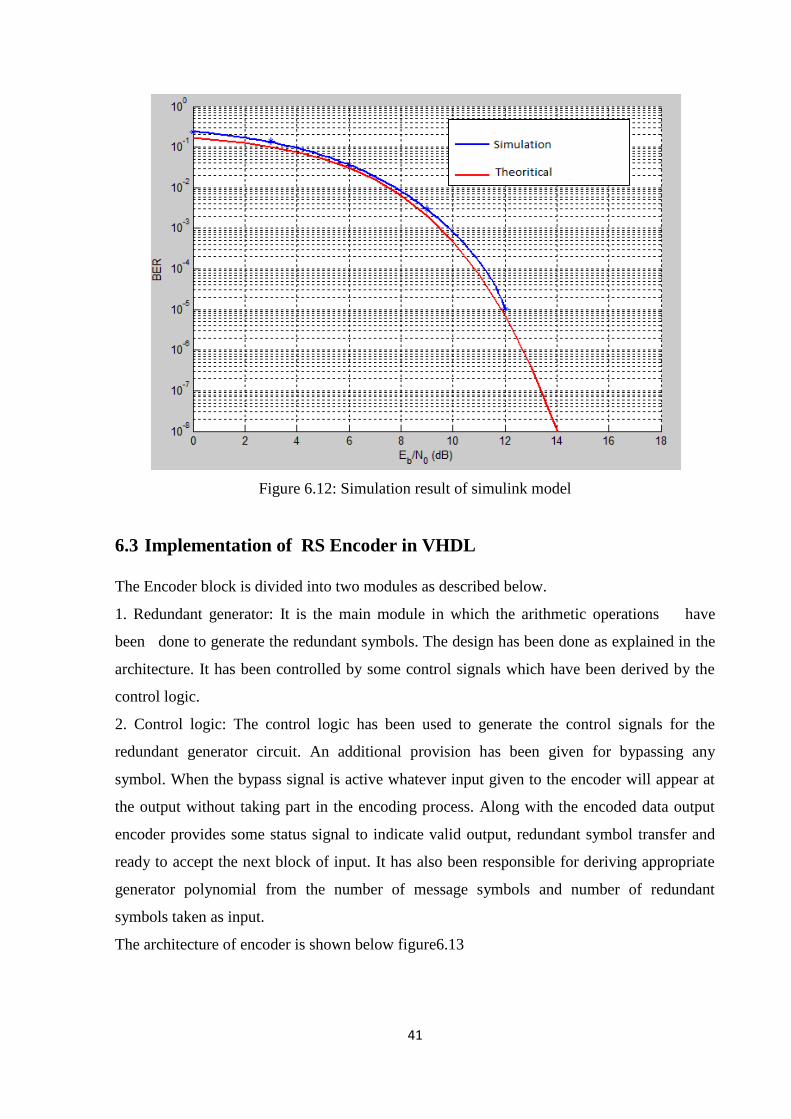
6.2 Implementation of RS Code in Simulink
A simulation model is constructed for analysis of performance of RS coding system over
AWGN channel is shown in figure 6.11. Then, simulating the model and extract BER
performance curve by using BERTool functions. The simulation result is shown in figure
6.12.
Figure 6.11: Simulation model for RS coding system
41
Figure 6.12: Simulation result of simulink model
6.3 Implementation of RS Encoder in VHDL
The Encoder block is divided into two modules as described below.
1. Redundant generator: It is the main module in which the arithmetic operations have
been done to generate the redundant symbols. The design has been done as explained in the
architecture. It has been controlled by some control signals which have been derived by the
control logic.
2. Control logic: The control logic has been used to generate the control signals for the
redundant generator circuit. An additional provision has been given for bypassing any
symbol. When the bypass signal is active whatever input given to the encoder will appear at
the output without taking part in the encoding process. Along with the encoded data output
encoder provides some status signal to indicate valid output, redundant symbol transfer and
ready to accept the next block of input. It has also been responsible for deriving appropriate
generator polynomial from the number of message symbols and number of redundant
symbols taken as input.
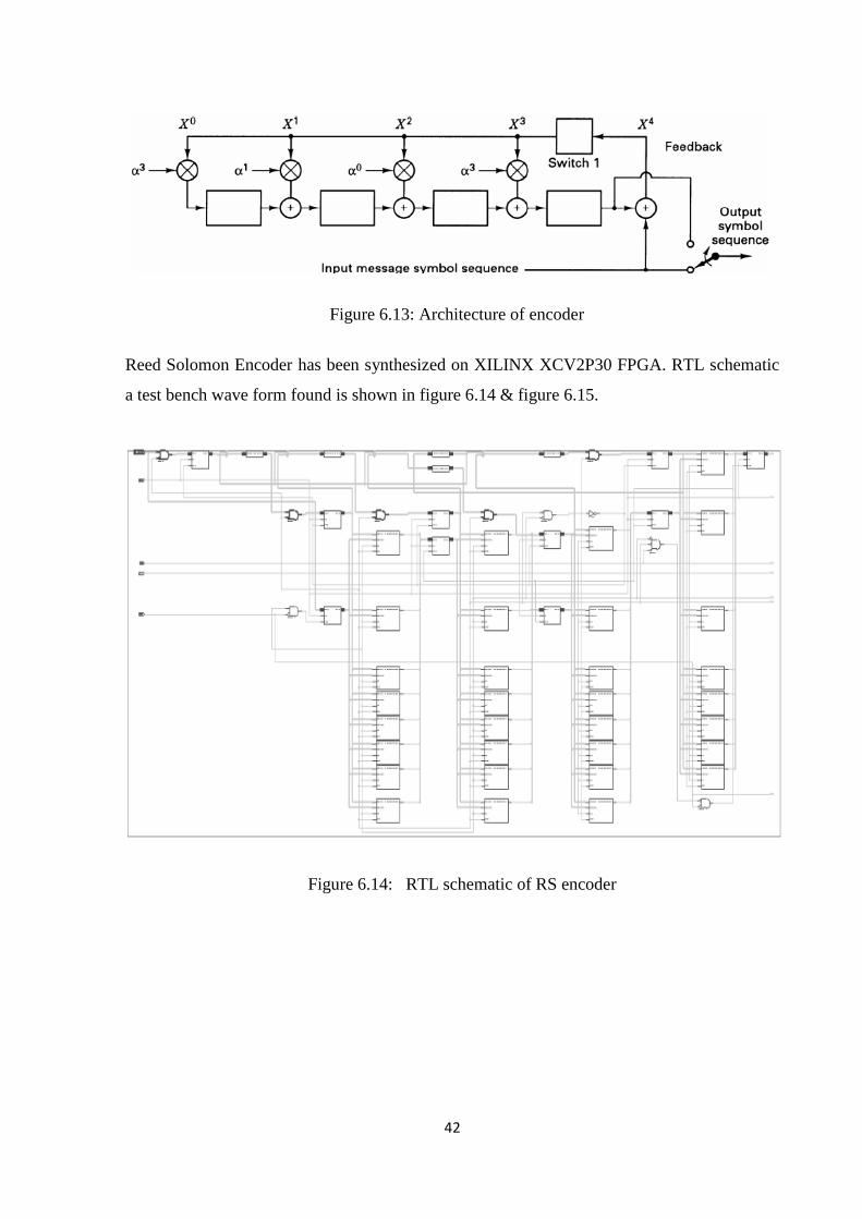
The architecture of encoder is shown below figure6.13
42
Figure 6.13: Architecture of encoder
Reed Solomon Encoder has been synthesized on XILINX XCV2P30 FPGA. RTL schematic
a test bench wave form found is shown in figure 6.14 & figure 6.15.
Figure 6.14: RTL schematic of RS encoder
43
Table 6.1 Device utilization in FPGA in RS encoder
In the figure 6.15 below we have taken the different signals RST(reset) . CLK-(clk signal),
STR-(start execution of program). RD-(data read out strobe). D_IN-(data input). D_OUT-
(data output). SNB(impulse when encoding is finished). pr231, pr210, pr30& pr116 are
Galois multiplier having primitive element.
Figure 6.15; Test bench wave form of RS encoder
The output of encoder data bit stream is found. 8bit data input 01011101.Output after
encoding of a single signal 01011101. No. of clock cycle 2m
-1equal to255 cycles. First k
cycles are used to move the data bit stream right ward and then next n-k bits are used to
encode the data using Read out strobe. Length of clock cycles 200ns For start bi tone time
equal to 51400ns . Read out strobe 4 clock cycles. Output after 51800ns, 258 clock cycles.
One clock cycle is error.
44
CHAPTER- 7
CONCLUSIONS AND FUTURE WORK
In this thesis the important characteristic of RS error correcting coding technique has
been discussed. Convolutional code process bit-by-bit, but block code like Reed-Solomon
code process on block-by-block basis. The actual maximum code rate allowed depends on
error-correcting code used. Reed-Solomon code are systematic code that is why actual
information appears unaltered in the encoded data, redundant bit are added for detection and
correction of error. Key idea behind Reed-Solomon code is data visualized as a polynomial.
Reed Solomon code was simulated in MATLAB. In encoder redundant symbols were
added using generator polynomial. Decoder error location and magnitude are calculated using
same generator polynomial. In RS(255,251) after encoding information remaining same
while extra 4-bit parity symbol are added. Before data transmission the encoder attached
parity symbol using a predefine algorithm. It was found that if the error is in parity symbols
even then the decoder is able to detect the output. The decoder first corrects the symbols and
then removes the redundant parity symbols from the code word and produces the original
input data. From the simulation result it has been shown that the decoder can correct upto ‗t‘
numbers of error.
The simulation result for MFSK with and without RS CODE graph between BER VS
SNR has been plotted. The error performance of the RS coding system has also been
calculated by the simulation model using SIMULINK. In the error probability graph, it was
seen that for a particular range of SNR, the number of error bits present can be found out
using the bit error rate probability. For different error correcting capabilities of RS code, the
range of SNR goes on increasing as the error correcting capability increases.
Reed Solomon Encoder has been implemented in VHDL synthesise is done on
XILINX XCV2P30 FPGA. RTL schematic has been found and a test bench has been written
to verify the functionality of the encoder. The output of the encoder is seem to be same as
input after 255 cycles, it will take only four bit parity. . In future, one can design the RS
decoder and then test this benchmark in a real time based example. One can also implement
this in an FPGA.
45
REFERENCES
[1] Sandeep Kaur ―VHDL Impletation of Reed-Solomon code,‖ Thesis, Thapar Institute
of Engg, 2006.
[2] Kanny Chung Chun Wai and Dr Shanchieh jay Yang ―Field Programmable Gate Array
Implementation of Reed—Solomon code, RS(255,239),‖http://www.ce.rit.edu/~sjyeec
/paper/workshop-rs-codec.pdf, Sept. 10, 2010.
[3] ― Error detection and correction,‖ http://en.wikipedia.org/wiki/Error_detection_and
_correction, July 20, 2010.
[4] Peter Sweeney, ―Error Control Coding: From Theory to Practice,‖ John Wiley & Sons,
Ltd., 2002.
[5] Richard E. Blahut, ―Theory and Practice of Error Control Codes,‖ Addison- Wesley,
1983.
[6] Stephen B.Wicker , ―Reed-Solomon code And Their Application,‖ IEEE Press, 1994.
[7] ―Reed-Solomon error correction,‖ http://en.wikipedia.org/wiki/Reed-Solomon_error
_correction, Jan. 11, 2011.
[8] Joel Sylvester, ―Reed-Solomon codes,‖ Elektrobit, Jan. 2001.
[9] Syed Mohd Fairuz Bin Syed Mohd Dardin, ―Evaluation of RS Coding performance for
M-ary modulation in AWGN and multipath fading channels,‖ Project Report,
University Teknologi Malaysia, Nov. 2005.
[10] Mark Haiman, ―Notes on Reed-Solomon Codes,‖ Feb. 2003.
[11] J. I. Hall, ―Notes on Coding Theory,‖ Dept. of Mathematics, Michigan State University,
East Lansing, MI 48824 USA, Jan. 3, 2003—―Chapter 5: Generalized Reed-Solomon
Codes‖ Internet Article, pp. 63-76, Jan. 3, 2003.
[12] Bernard Skalar and Pabritra Kumar Ray, ― Digital Communications: Fundamentals &
Applications,‖ Pearson, Edition 2, Jan. 2009.
46
[13] Proakis John G., Salehi M., ― Communication System Engineering,‖ Prentice Hall of
India, Edition 2,2005.
[14] Peter J. Cameron, ―Galois Fields,‖ The Encyclopaedia of Design theory, May 30, 2003.
[15] ―Reed-Solomon(RS) Coding Overview,‖ VOCAL Technologies, Ltd., Rev. 2.28n,
2010.
[16] J.Y Chang and C. Shung, ― A high speed Reed-Solomon codec chip using look forward
architecture,‖ IEEE APC CAS‘94, PP. 212-217, Dec. 1994.
[17] Lee H., ―A high speed, low complexity Reed-Solomon decoder for optical
communications,‖ IEEE Transactions on Circuits and Systems II, PP. 461-465, 2005.
[18] J.Bhasker, ―A VHDL PRIMER,‖ Prentice-Hall India, Edition 3, 1998.
[19] Peter J. Ashenden, ―The Designer‘s Guide to VHDL,‖ Morgan Kaufmann Publishers,
Edition 2, 2004.