Embed Size (px)
Citation preview
Proceedings of the Seventh Federal Interagency Sedimentation Conference, March 25 through 29, 2001, Reno, NV
Volume 2
VI. Data QualityAssurance
Dat
a Q
ualit
y A
ssur
ance

Proceedings of the Seventh Federal Interagency Sedimentation Conference, March 25 through 29, 2001, Reno, NV
VI. Data Quality Assurance
TABLE OF CONTENTSPage
ACCURACY, CONSISTENCY, AND RELIABILITY OF SEDIMENT MEASUREMENT ANDMANAGEMENT AND THEIR COSTS: Liu Chuang, USDA-NRCS, Washington, DC
VI – 1
A SPREADSHEET ANALYSIS OF SUSPENDED-SEDIMENT SAMPLING ERRORS: John V.Skinner, USGS (retired), Seymour, IN
VI –9
COMPUTATION OF SUSPENDED-SEDIMENT CONCENTRATIONS IN STREAMS: David J.Holtschlag, USGS, Lansing, MI
VI – 17
DATA MINING AND CALIBRATION OF SEDIMENT TRANSPORT MODELS: Peter G. Waldo,USDA-NRCS, Fort Worth, TX
VI – 25
A PROBABILITSTIC APPROACH TO MODELING EROSION FOR SPATIALLY-VARIEDCONDITIONS: W. J. Elliot, P. R. Robichaud, and C. D. Pannkuk, USDA-FS, Moscow, ID
VI – 33
SEDIMENT LABORATORY QUALITY-ASSURANCE PROJECT: STUDIES ON METHODS ANDMATERIALS: J. D. Gordon, USGS, Vancouver, WA; C. A. Newland, USGS, Lakewood, CO; and J.R. Gray, USGS, Reston, VA
VI – 41
GCLAS: A GRAPHICAL CONSTITUENT LOADING ANALYSIS SYSTEM: T. E. McKallip and G.F. Koltun, USGS, Columbus, OH; J. R. Gray and G. D. Glysson, USGS, Reston, VA
VI – 49

Proceedings of the Seventh Federal Interagency Sedimentation Conference, March 25 to 29, 2001, Reno, Nevada
VI - 1
ACCURACY, CONSISTENCY, and RELIABILITY of SEDIMENT MEASUREMENTand MANAGEMENT, and THEIR COSTS
Liu Chuang, Senior Program Analyst, Natural Resources Conservation Service, U.S.Department of Agriculture, Washington, D.C.
Liu Chuang, Room 6162, USDA South Building, phone: 202-720-7076, fax: 202-720-6473,[email protected]
INTRODUCTION
This paper aims to use one example of sediment measurement to convey the basic concepts ofeconomic reasoning. Sediment measurement program is chosen for its general familiarity amongparticipants in this conference.
Sediment is a phenomenon of soil erosion process, which generally starts with soil first beingdetached by wind or water, or other forces, then further transported and finally either becomessuspended particles in water or wind and finally settled on land surface. Sediment represents thesoil quantity suspended or deposited.
Sediment has been cited to be the number one threat to American water quality. Sedimentimpairs fish respiration, plant productivity, and ecosystems of other marine life, and furtherlimits the aesthetic, transportation, hydro-power and recreational usefulness of rivers and lakes.
Sediment information is used for measuring effects of changing agricultural practices, forengineering design of facilities, such as bridges, locks, dams, and hydropower structures, forreservoir study to help reservoir maintenance.
Measurement of sediment, like measurement of any other physical or non-physical matter andvariables, always aims to provide accurate, consistent, and reliable estimates for users orpotential users.
Accuracy on sediment measurement means measured sediment is close to actual amount ofsediment one intends to measure, or the difference between sediment actually measured and thesediment intended to be measured becomes the minimum. In statistical terms, unbiasedestimator of sediment measurement satisfies the requirement of accuracy.
Consistency on sediment measurement means methods and procedures used to measure sedimentin different time and location should be the same, so comparison among the measured sedimentvalue in different locations and times could be consistently compared. Consistency in statisticalterms means that estimates of true sediment in a sample become closer to the true value ofsediment when sample size becomes larger, or the variance of an estimated sediment valuebecomes smaller when the sample size increases.

Proceedings of the Seventh Federal Interagency Sedimentation Conference, March 25 to 29, 2001, Reno, Nevada
VI - 2
Reliability has been used interchangeably with precision. It means that under same conditions ofmeasurement, the method and procedures of sediment measurement would yield estimates of theexpected value of the true sediment value repetitiously. In other words, it means an estimatefrom a more reliable estimator would have a higher probability of being close to the expectedvalue than an estimate from a less reliable estimator. In general statistical terms, one would saythat within a given interval, a more reliable estimator has less chance of producing an estimateoutside of that interval than a less reliable estimator.
In principle the more accurate, consistent, and reliable sediment measurement, the larger asample size and more effort will be needed. The more effort for sediment measurement meansthat more investment in resources for measurement and these include effort, human hours,instruments and materials. This will increase the costs of measurement.
THE FACTOR INPUTS AND PROCEDURES FOR SEDIMENT MEASUREMENT
Sediment data collection and management are just a small part of the earth-science data forwhich the USGS and other associated agencies and institutions are responsible. Sedimentmeasurement involves several major tasks. These are 1) to monitor sediment transport instreams by collecting water samples at selected sites, 2) to measure suspended-sedimentconcentration in water, then 3) to estimate total suspended-sediment load flowing past a site, then4) to publish information and data, and 5) to circulate and distribute these data and informationto users.
In order to do the tasks described above, USGS and responsible agencies need to buildmonitoring stations and hire sediment observers in the country. Several steps are needed to buildthe monitoring stations. Planning and decision on site selection will first be made. Constructionand installation of the monitoring site will then follow with the inspection and testing of theinstruments. Simultaneously, sediment observers will be hired and trained by the USGSpersonnel.
The cost components of the sediment measurement primarily will consist of the following items:A monitoring stream gagging shelterMechanical/electronic instruments in a shelter near stream will include:
Wire-weight gage (a drum with single layer of cable, bronze weight, a graduateddisc, a counter, and a aluminum box)Sediment sampler box,Suspended sediment sampler,Staff gage (monitor elevation/gage height of water on site)
Personnel of USGS do regular site visits at least every 6 weeks to (1) collect samples at the gagehouse or a specific site, and (2) restock supply of bottles, nozzles, gaskets, log sheets, markers,thermometers, or other supplies. They also conduct the analysis of the data being collected. Tobe more specific, to operate and maintain the site the USGS personnel have basic duties such as

Proceedings of the Seventh Federal Interagency Sedimentation Conference, March 25 to 29, 2001, Reno, Nevada
VI - 3
1) To inform the sediment observer of the sampling strategy to follow at the site, like afixed schedule (per day, per week, or month), or a schedule based on water discharge(like, sample 3 times per day during floods), and .
2) To provide supplies needed by the sediment observer to consistently collect accuratewater sample and data.
3) To collect water samples (measure suspended sediment concentration (mg/l)) and tore-supply periodically for the monitoring station.
4) To estimate mean discharge, mean concentration, sediment discharge, and othervariables as requested.
5) To publish the data, and circulate/distribute to audiences
In general, more samples will be collected during floods. These samples are critical to measureand compute, as well as to publish sediment records at these sites. Water sample collection byUSGS sediment observer will involve a set of standard procedures. An observer would spendapproximately 15 minutes per site per sampling. This results in about 5 hours per month actualtime spent at each gage. This estimate does not include driving time. In general, an observerwith one station receives $100 per month to collect 3 sample per week, and an additional samplefor additional $7.50.
USGS pays the sample observer every 3 months or quarterly. Sediment observers should neverrisk injury to collect samples, and can call collect any time to USGS personnel on any concernsrelated to sampling. However, if there is an accident related to water sampling by the observer,USGS might have difficulty to escape responsibility for part or whole of the associated remedies.
THE PRODUCTION FUNCTION FOR SEDIMENT MEASUREMENT ANDINFORMATION PRODUCTION
From the above discussion and explanation of the factor inputs and processes needed forproducing sediment information, a simple production could then be hypothesized as follows:
Input in labor hour (L) includes:
• Staff time of USGS personnel in planning, contracting, inspecting, managing, andprocessing the payments to any contractors for site construction and installation, andprocurement of supplies (L1).
• Staff time in hiring, training the sediment observer and in analyzing and processingsediment data for users (L2).
• Sediment observers’ time to collect and record the water sample (L3).
Fixed and variable material capital inputs (K) include:

Proceedings of the Seventh Federal Interagency Sedimentation Conference, March 25 to 29, 2001, Reno, Nevada
VI - 4
• Fixed capital investment in monitoring site evaluation, planning, and construction of themonitoring site (K1).
• Mechanical and electronic instruments (K2)• Variable supplies for the site and monitoring activities (K3).
Management and technological factor input (A, B) will take into account the evaluation andselection of the site and all instruments, the design of all instruments used, and the knowledgeand skills in the development and integration of all the personnel and material components.
Assuming S is the data and information of sediment report, then the above inputs for sedimentmonitoring could be structured into a simple production function as follows:
S= f (K, L)=AK+ BL
Where S= sediment data and information including mean discharge, sediment discharge,mean concentration, temperature, and others.
A and B are technology coefficient vectors for capital and labor, where A=A1, A2, andA3; B=B1, B2, and B3.K, the capital inputs including both fixed (shelter site) and variable capital (instruments
andsupplies), where K=K1 +K2 +K3L, the labor hours of all sediment management personnel and observers, sum of all laborhours, where L=L1+L2+L3.
The production function, as one can observe, is a technical or engineering relation betweenoutput and inputs. For any given set of inputs, the production processes are designed to yield thegreatest output. Economists or engineers are interested in finding the maximum output for anygiven set of inputs in the production function.
Output, in our example here is the flow of sediment data and information generated by thecombined efforts of all the personnel and material investment involved. The data andinformation of sediment could be expressed as an indexed output. Output could also beexpressed as multi-products, such as water height, temperature, mean discharge, meanconcentration, and sediment discharge. Material capital inputs could be considered as stock orflow concepts and they could be more than one kind as discussed previously. The same situationexists among different kinds of labor as expressed in labor hours that are flow concepts.
As technology changes, the parameters of the production function would also change. In a worldof progress, both capital and labor quality would change along the time. Therefore, thehypothesized production function could be rewritten into the following:
S= F (K, L, A, B, t)
Where t is time, or time period,

Proceedings of the Seventh Federal Interagency Sedimentation Conference, March 25 to 29, 2001, Reno, Nevada
VI - 5
S is the sediment output in time,K is the capital input in time,L is the labor input in time.
Data used to estimate parameters in the hypothyzed production function could come from timeseries or cross sectional data. Time series are from daily, monthly, quarterly and yearly data ofboth output and input series. Cross sectional data could come from, in our example, differentsediment measurement stations across the country.
MINIMIZING THE ECONOMIC BURDEN OF SEDIMENT MEASUREMENT
Although no prices are given to the value of sediment measurement, and USGS is not selling thedata for profit, we still could have a hypothetical or “shadow” price for the unit value of thesediment measurement to derive the expected total value of the sediment information for thecountry. The cost function of the sediment measurement will be derived from the productionfunction we discussed. However, in a governmental setting, where the expected total cost of thesediment measures would be like any governmental project, it makes sense to minimize total costfor any given output of the sediment measures. By definition, the total cost will be the sum of alllabor costs, capital costs and material cost together. Since we define 3 kinds of labor, thereshould have 3 levels of wages. Likewise, 3 kinds of capital will have 3 kinds of rental rate forthem.
Minimize total cost C=w1L1 +w2L2 +w3L3+K1r1+Kr2+K3r3
Subject to production constraints where S = f (K, L)=AK+ BL (1)S is a given set of sediment measurementK=K1+K2+K3L=L1+L2+L3A=[A,A2,A3); B=[B1,B2,B3]
Ratios of factor costs = ratios of corresponding marginal productivityW1/W2=f’(L1)/f’(L2) (2)W1/W3= f’(L1)/f’(L3) (3)W1/r1=f’(L1)/f’(K1) (4)W1/r2=f’(L1)/f’(K2) (5)W1/r3=f’(L1)/f’(K3) (6)
There are 7 equations and are 7 unknowns. These equations could be transformed into a formthat a production input such as labor and capital is a function of a set of factor price ratios plusthe level of sediment measurement, such as L1=f1(w1/w2, w1/w3, w1/r1, w1/r2, w1/r3, S).
By multiplying individual cost rate (wage, or capital price) to the above equation, the aboveequation becomes: w1L1=w1f1(wage and capital rate ratios and S). The same procedure isapplied to the other 5 equations to provide similar types of equations. Then, by summing all the5 equations to derive the total cost function for sediment measurement as follows:
C=F (w1, w2, w3, r1,r2, r3, S)
Proceedings of the Seventh Federal Interagency Sedimentation Conference, March 25 to 29, 2001, Reno, Nevada
VI - 6
The total cost therefore is a function of factor unit costs and total level of sediment measurement.The supply function of each factor for sediment measurement is equivalent to the marginal cost(MC) function of the total cost function, which can be expressed as L1=MC (individual factorunit costs, and the total unit cost of the sediment measurement.)
In order to minimize the total cost of the sediment measurement under a determined level ofsediment measurement, the conditions should be observed:
Ratios of factor costs = ratios of corresponding marginal productivity.Or, the value of marginal product of an input, like L1, should be equal to thevalue of marginal product of every other input used in the production of S.
For example: If the wage rate of USGS personnel is $40 per hour, while the wage rate ofsediment observers is $20 per hour (as reported $100 for 5 hours in average), the unit cost ratioof these two types of labor input is 2. The ratio of having an incremental increase in sedimentmeasurement by hiring additional USGS personnel and the incremental increase in sedimentmeasurement by an additional sediment observer should be 2. In other words, the additionalsediment measurement of a USGS personnel should be at least 2 times that of an sedimentobserver, otherwise it would not be economical.
In order to increase the accuracy, consistency and reliability of sediment measurement, moresamples or more sediment measurement will need to be taken. This could come from hiringmore sediment observers, increasing USGS supervisory and analytical personnel on the project,or building more sediment monitoring stations. For considering these options, the economic ruleof thumb suggests that the unit cost ratios of each pair of factor inputs should be equal to theratios of incremental sediment measurement information made with respect to the correspondingpaired factor inputs.
ECONOMIC BURDEN AND REQUIREMENTS OF SEDIMENT MEASUREMENTS
Accuracy versus economic burden
Accuracy in sediment measurement means unbiased measurement in statistical terms. Let S’ bethe estimator of the hypothetically true sediment measurement S, two conditions should be met.The expected value of S’, or E(S’), should be equal to S. When the frequency of measurementreaching infinity, the expected value of sediment measurement will be equal to its hypotheticalvalue. By definition in mathematical term, the accuracy or unbiased measurement could bewritten in the following equations:
E(S’) = S (1)
E(S’) = ∫∞
∞S’f (S’) dS’ (2)
By definition of Equation 2 above, when frequency of measurement is large, then the measuredaverage sediment will be equal or approximately approach to the true sediment measure thesediment design has been looking for.

Proceedings of the Seventh Federal Interagency Sedimentation Conference, March 25 to 29, 2001, Reno, Nevada
VI - 7
To increase the frequency of sediment measurement we will have to require the sedimentobserver to get more water samples than originally agreed or planned. The implication of therequirement for accuracy is a higher variable cost of sediment measurement. Variable costelements will include the hours spent by sediment observers, the USGS personnel time ofmonitoring and supervising the monitoring stations, the supplies such as water bottle, log paper,and markers. Frequent use of the fixed components of the monitoring stations will increase thedepreciation of the instruments installed for the monitoring activities. The potential increase offailure rate of these instruments and equipment, the reliability of the monitoring station will bedecreased.
Therefore, in the onset of the monitoring design it will be critical to decide the frequency andtiming of water sample collection, especially in the planning stage. Good effort on this criterionwill produce a better plan, better data for requesting needed budget, and certainly will yield moreaccurate estimate of the average sediment estimates for each station.
Consistency and reliability versus economic burdenConsistency means if the sediment average measures tend to become concentrated on the truevalue of the sediment average, or the hypothetically expected sediment average, the sedimentmonitoring station has been designed for. Consistency means that when sample size increasesthe estimated sediment average become closer to its true average, or become a more reliableestimate of the true value.
When an estimate is consistent, it becomes an efficient estimate with less variation, and it alsobecomes a more reliable estimate because the chance of accepting an false estimate as well asrejecting a true estimate becomes smaller. Therefore, consistency requires another statisticalcondition, that the variance of an estimate, S’, should becomes smaller and smaller when thesample size becomes bigger and bigger.
Var (S’) < Var (S’’), where S’’ is alternative estimators of the sediment.
In brief, to gain more consistent and reliable estimates of the sediment averages, the sample sizeshould be larger. Therefore, the cost, especially the variable cost of the monitoring activities ofsediment will increase.
Reliability
Reliability is a statistic that shows the probability of having true value of sediment measuredwithin a certain percentage range of the estimated sediment value, like 5%. This statistic is acomponent of accuracy and closely related to consistency of an estimated sediment value. Oncethe bias and distribution of a estimated sediment value have been determined, the predictivepower, or reliability of the estimated sediment value of its true value can then be determined. Toincrease sample size will not only increase the accuracy and consistency of an estimate, but alsothe reliability of the predictive power of the measured sediment value. As we have discussedabove, the increase of sample size certainly will increase the costs of sediment measurement.However, by choosing to measure more samples within a flooding period, fewer samples withina slow flow period from a stream, the sample design basically reduces the variance of the

Proceedings of the Seventh Federal Interagency Sedimentation Conference, March 25 to 29, 2001, Reno, Nevada
VI - 8
estimated sediment value, and hence enhances its predictive power, or reliability, in estimatingthe true value of sediment.
CONCLUSIONS AND RECOMMENDATIONS
To increase accuracy, consistency and reliability of measuring suspended sediment in water,more sampling or larger samples in general will be needed.
Since sediment measurement is a public endeavor rather than a profit maximization activity,economic conditions for profit maximization will not be applied. Instead, cost minimizationconditions by subjecting the total cost function to be under constraints of different levels ofmarginal productivity of sediment measurement should be considered.
The crucial economic conditions for weighing the choices of action to increase the frequency ofwater sampling and analysis activities are the ratios of unit cost of factor inputs for the sedimentmeasurement. These factor inputs could be the estimated labor hours of USGS supervisory andanalytical personnel and that of sediment observer, and the rental rate or cost of capitalinvestment in water monitoring station and its associated electronic instruments as well asneeded material supplies.
For better design in order to derive more consistent, unbiased, and reliable estimates of sedimentmeasurement, it is crucial to incorporate the expected statistical parameters the audience or usersof these measures consider acceptable. Also, the pre-knowledge and analysis of the productionand cost function of entire set of measurement stations and their administrative and managementsupport, and the trade-off in cost and productivity among all factor inputs in the sedimentmeasurement system should be crucial in helping reducing costs of the sediment measurement.
REFERENCES
Bain, Lee J., Introduction to Probability and Mathematical Statistics, 1987, Duxbury Press,PP.58-59, PP.276-278, PP.283-284.
Johnson, Gary P. 1997, Instruction Manual for U.S. Geological Survey Sediment Observers, U.S.Geological Survey, Open-File Report 96-431.
Klein, Lawrence R., 1962, An Introduction to Econometrics, Prentice-Hall, Inc.PP.84-129
Liebhafsky, H. H., The Nature of Price Theory, 1963, the Dorsey Press. Inc., PP.119-194.
Mood, Alexander M., Graybill, Franklin A. Introduction to the Theory of Statistics, 1963,McGraw Hill Book Company, Inc. PP.172-175; PP.311-318; 248-334.
Scheaffer, Richard L, Mendenhall, William, and Ott, Lyman, 1990, Elementary SurveySampling, Duxbury Press, PP.90-97.

Proceedings of the Seventh Federal Interagency Sedimentation Conference, March 25 to 29, 2001, Reno, Nevada
VI - 9
A SPREADSHEET ANALYSIS OF SUSPENDED-SEDIMENTSAMPLING ERRORS
By John V. Skinner, Hydrologist8129 Andreas Path, Seymour, IN 47274
Abstract: Accurate sampling of suspended sediment requires special conditions at the entranceof an upstream facing nozzle. Flow velocity within the nozzle must match the upstream velocityin the proximity of the opening. Unfortunately, meeting this exacting requirement is seldompossible. This paper presents a method for evaluating sampling errors at a single vertical in aflow cross-section. A popular spreadsheet format is used to analyze four hypothetical samplerswith abnormal inflow characteristics. They are evaluated under three flow regimes and foursizes of sediment particles. The data verify the importance of using samplers with idealcharacteristics. Among the hypothetical samplers, the one with excessively high intake rates issuperior to those with abnormally low rates. Errors are greatest with the largest grains(0.45mm) moving in low flows.
INTRODUCTION
Assessing errors in sampling suspended sediment is difficult for users as well as designers ofsampling equipment. Errors arise from many sources that include inadequate coverage oftemporal and spatial variations in sediment discharge. The frequency of sampling must beadequate to document the most rapid changes in discharge. Spatial sampling must be adequate toaccount for point-to-point variations in sediment distribution within a river cross section. Thisreport addresses another aspect of errors, namely their relation to intake characteristics ofsamplers. With growing diversity in sampling requirements, designers and users alike mustsometimes embrace equipment with intake (filling rate) characteristics that are less than ideal.This report presents a method for estimating errors in depth integrating a single vertical. Themethod is applied to four hypothetical samplers with distinctly different intake characteristics.
In isokinetic sampling, flow approaches and then enters a sampler's nozzle without undergoingacceleration. Neither the speed nor direction of flow changes as water is captured and routed tothe sampling container. In non-isokinetic sampling, errors arise from two sources stemming fromdischarge biasing and particle momentum. With discharge biasing, a point in a verticalcontributes to a sample but the contribution is not proportional to the discharge at the point. Inother words, the contribution is not velocity weighted. Regions of low flow may contributedisproportionately large fractions to a sample while regions of high flow contribute smallfractions. The other error, particle momentum, stems from curvatures in streamlines as wateraccelerates to enter a nozzle. If inflow is hyperkinetic (nozzle flow exceeds approach velocity),streamlines converge on the nozzle but sediment particles, owing to their momentum, resist theconverging forces and escape capture. Consequently, sediment concentration in the sample fallsbelow that in the approaching flow. The action reverses in hypokinetic sampling when inflow isslower than approach velocity. In this case, sample concentration is erroneously high.
A sampling-error study conducted by the Federal Interagency Sedimentation Project (FISP,Report 3,1941) addressed discharge biasing but neglected particle-momentum errors. Later, data

Proceedings of the Seventh Federal Interagency Sedimentation Conference, March 25 to 29, 2001, Reno, Nevada
VI - 10
on momentum effects were published (FISP, Report 5, 1941). The present report incorporatesthe momentum data in an error analysis, which is presented in a popular spreadsheet format.
The particle-momentum experiment was conducted in a recirculating flume filled with water andsediment particles sieved into narrow size ranges. The test section was fitted with two upstream-facing nozzles mounted side-by-side and symmetrically located in the test section. One nozzlewas siphoned at isokinetic intake rates while the other was siphoned at rates ranging fromhyperkinetic through isokinetic to hypokinetic. One at a time, four grain sizes of sediment weretested: 0.45, 0.15, 0.06 and 0.01 mm. Error data were presented as graphs, which have beenconverted to power-series equations for use in the spreadsheet. Figure 1 shows plots of theequations.
Figure 1--Particle-momentum sampling errors
In figure 1, relative sampling rate is the intake rate of the test nozzle divided by the isokineticrate. Hyperkinetic rates plot to the right of 1.0; hypokinetic rates to the left. On the vertical axis,concentration errors are in percent with zero error occurring at a relative rate of 1.0. Errors arelargest for the biggest grains, 0.45 mm. Errors are nearly insignificant at all relative samplingrates for the smallest grains, 0.01 mm. Within each grain size, errors are larger for hypokineticrates than for hyperkinetic rates.
-40
-20
0
20
40
60
80
100
120
140
160
0 1 2 3 4 5 6
Relative Sampling Rate
Co
mp
ute
d C
on
cen
trat
ion
Err
or
in P
erce
nt
0.45 mm particles
0.15 mm particles
0.06 mm particles
0.01mm particles

Proceedings of the Seventh Federal Interagency Sedimentation Conference, March 25 to 29, 2001, Reno, Nevada
VI - 11
A sampler's intake characteristic is important in that it shows intake rates at various depths alonga sampling vertical. Intake measurements are usually made in a laboratory flume. Waterdischarge is stabilized then flow velocity is measured at a test point chosen to minimizeinterference from the flume walls and surface waves. The current meter is then removed and thesampler is held at the test point for a measured time interval. After retrieving the sampler, thevolume of water collected is measured. Intake rate is computed from the volume, the samplinginterval and the cross-sectional area of the nozzle. Intake rate is plotted opposite the approachvelocity, then flume discharge is set to a new level and the process is repeated. Duringdevelopment of a new sampler, intake characteristics are charted through a broad range ofapproach velocities, but once a sampler is in production, quality-control checks are usually madeat only one or two points.
When a sampler operates at depths of several meters, as during actual river sampling, stringentcontrols must be observed to insure its intake characteristics apply. Descent speeds must allowfor pressure equalization otherwise water floods the air-exhaust tube which, during properoperation, vents air from the sample container as water enters through the nozzle. Excessiverates of descent or ascent also create strong vertical currents, which interfere with smoothentrance flows. Limits on lowering and raising speeds, which are discussed in FISPpublications, constrain a sampler's operating depth. Throughout this paper, it is assumed intakecharacteristics govern sampling operation at all depths.
Four hypothetical intake characteristics are shown in figure 2 and are analyzed in thespreadsheet. Scales on figure 2 are in ft/s to aid readers in comparing intake-characteristic plotsin FISP publications. Units of ft/s can be converted to m/s by multiplying by 0.3048. On figure2, an ideal sampler plots as "SI" with intake velocities matching approach velocities through abroad range. Points falling above the SI line are hyperkinetic: points below are hypokinetic.Sampler SL is hypokinetic through its full range. Furthermore, it stops sampling approachvelocities slower than 1.5 ft/s (0.45 m/s). For approach velocities faster than 0.6 m/s, intake ratesplot parallel to the ideal line, SI. Sampler SL has characteristics similar to some bag samplers inwhich stiffness of the bag prevents inflow in slow moving water. Sampler SR is also similar tosome bag samplers that refuse to sample slow-moving water but are compensated throughhyperkinetic operation at high velocities. This performance is achieved by creating strongsuction pressures outside the bag. Sampler SF has an inflow velocity of 1.5 ft/s (0.45 m/s) inslack water. This operation is typical of many depth-integrating samplers, which have air-exhausts tubes opening above the intake nozzles. The intake of SF falls below the ideal forapproach velocities higher than 3ft/s (0.9m/s). Sampler SH also samples in slack water but,unlike SF, it is hyperkinetic throughout its entire range. The four test samplers, SL, SF, SH andSR suffer from deficiencies that, for purposes of comparison, exaggerate shortcomings ofproduction samplers. Characteristics of samplers in the U.S. series deviate from the ideal byonly a few percent.

Proceedings of the Seventh Federal Interagency Sedimentation Conference, March 25 to 29, 2001, Reno, Nevada
VI - 12
Figure 2--Intake characteristics of hypothetical test samplers
COMPUTATIONAL METHOD
The initial step in computing sampling errors is to assign constants listed in column A of thespreadsheet (figure 3). The first entry is the sampler type, SF in this case. The note is areminder to enter the intake characteristic in equation form in all cells of column J. Returning tocolumn A, the following parameters are listed in order (a) the sediment concentration at thestream bottom, (b) the fall velocity of the particle-size class, (c) Manning's roughness coefficient,(d) stream depth at the sampling vertical, (e) mean velocity in the vertical, (f) entrance diameterof the sampling nozzle and (g) the sampling interval in seconds for each segment of the vertical.
In the computations, the vertical is arbitrarily divided into twenty segments. As anapproximation, velocities and concentrations are assumed equal at all points within a segment.Accuracy of the approximation can be improved at the expense of using more segments andworking with larger spreadsheets. The segments are listed in column B with their boundariesshown as fractional depths with zero at the water surface and 1.0 at the stream bottom. Column C
0
1
2
3
4
5
6
7
8
9
10
0 2 4 6 8
A, Approach Velocity in Feet per Second
I, In
take
Vel
ocity
in F
eet p
er S
econ
d
SH
SL
SR
SF
SI

Proceedings of the Seventh Federal Interagency Sedimentation Conference, March 25 to 29, 2001, Reno, Nevada
VI - 13
Spreadsheet for SF Sampler, 0.45-mm Sediment and Low Flow
123456789
1011121314151617181920212223
2425262728
A B C D E F G H I J K L M
ASSIGNED CONSTANTS f, F
ract
iona
l dep
th a
t sam
plin
g ve
rtic
al (
0 is
sur
face
, 1is
bot
tom
)
Rel
ativ
e he
ight
of s
egm
ent
boun
darie
s ab
ove
stre
am b
ed
Str
eam
vel
ocity
at s
egm
ent
boun
darie
s, ft
/s.
A, A
vera
ge v
eloc
ity in
seg
men
t. A
lso
idea
l sam
pler
ave
rage
inta
ke
velo
city
, ft/s
Q, F
or id
eal s
ampl
er, v
olum
e of
sa
mpl
e co
llect
ed in
inte
rval
, ml
Sed
imen
t con
cent
ratio
n at
seg
men
t bo
unda
ry, m
g/L
Ave
rage
con
cent
ratio
n in
seg
men
t. A
lso
for
idea
l sam
pler
, con
cent
ratio
n of
sam
ple
in s
egm
ent,
mg/
L
For
idea
l sam
pler
, mas
s of
sed
imen
t co
llect
ed in
seg
men
t, m
g
Inta
ke V
eloc
ity o
f tes
t sam
pler
(T
S),
ft/
s
Vol
ume
of s
ampl
e co
llect
ed in
in
terv
al b
y T
S, m
l
Rel
ativ
e sa
mpl
ing
rate
for
TS
Sed
imen
t con
cent
ratio
n er
ror
for
TS
, pe
rcen
t
0.00 1.00 2.63 0.000.05 0.95 2.60 2.62 25.27 0.00 0.00 0.00 2.81 27.12 1.07 -2.41
No, Sediment Concentration at Stream Bottom, mg/L 0.10 0.90 2.57 2.58 24.94 0.00 0.00 0.00 2.79 26.96 1.08 -2.591000 0.15 0.85 2.53 2.55 24.60 0.00 0.00 0.00 2.77 26.79 1.09 -2.79
c, Fall Velocity of particles, cm/s. 0.20 0.80 2.49 2.51 24.25 0.00 0.00 0.00 2.76 26.61 1.10 -3.007.6 0.25 0.75 2.45 2.47 23.86 0.01 0.01 0.00 2.74 26.42 1.11 -3.23
n, Manning roughness coefficient 0.30 0.70 2.41 2.43 23.45 0.02 0.01 0.00 2.71 26.21 1.12 -3.480.04 0.35 0.65 2.36 2.38 23.02 0.04 0.03 0.00 2.69 25.99 1.13 -3.76
D, Stream depth at sampling vertical, ft. 0.40 0.60 2.31 2.33 22.55 0.08 0.06 0.00 2.67 25.76 1.14 -4.063 0.45 0.55 2.25 2.28 22.04 0.18 0.13 0.00 2.64 25.50 1.16 -4.40
Vm, mean velocity in vertical, ft/s 0.50 0.50 2.19 2.22 21.48 0.39 0.28 0.01 2.61 25.22 1.17 -4.782 0.55 0.45 2.13 2.16 20.87 0.86 0.62 0.01 2.58 24.92 1.19 -5.21
d, sampler nozzle diameter, in. 0.60 0.40 2.05 2.09 20.18 1.87 1.36 0.03 2.55 24.58 1.22 -5.710.25 0.65 0.35 1.97 2.01 19.42 4.11 2.99 0.06 2.51 24.19 1.25 -6.30
T, sampling time in each segment, s. 0.70 0.30 1.87 1.92 18.54 9.01 6.56 0.12 2.46 23.75 1.28 -7.011 0.75 0.25 1.76 1.81 17.51 19.75 14.38 0.25 2.41 23.24 1.33 -7.88
0.80 0.20 1.61 1.68 16.27 43.29 31.52 0.51 2.34 22.62 1.39 -9.000.85 0.15 1.43 1.52 14.71 94.91 69.10 1.02 2.26 21.84 1.48 -10.540.90 0.10 1.18 1.30 12.59 208.07 151.49 1.91 2.15 20.78 1.65 -12.830.95 0.05 0.74 0.96 9.23 456.15 332.11 3.07 1.98 19.10 2.07 -16.911.00 0.00 0.00 0.37 3.56 1000.00 728.08 2.59 1.68 16.26 4.57 -27.12
Total volume
collected by ideal sampler,
ml388.33
Total sediment
mass collected by ideal sampler,
mg 9.58
Total volume
collected by test
sampler, ml
483.85
24.66 39.73
Sampler type--SF. Insert intake characteristic equation in column J.
Concentration of sample collected by ideal sample, rmg/L
Concentration of sample collected by test sampler, mg/L
Figure 3—Sample spreadsheet for sampling errors in a vertical.

Proceedings of the Seventh Federal Interagency Sedimentation Conference, March 25 to 29, 2001, Reno, Nevada
VI - 14
inverts the segment designation to simplify certain computations. The value 1.0 now designatesthe water surface and "0" the stream bottom.
Stream velocities at segment boundaries are computed in column D from the following velocityequation extracted from Report 3 (FISP, Report 3, 1941):
V = Vm [1+(9.5n/D 1/6)(1+loge h)] (1)
Where:V is stream velocity at h,Vm is mean velocity in the vertical,n is Manning's roughness coefficient,D is stream depth at the vertical, andh is the ratio of the distance to a point above the streambed to the total depth at thevertical.
Equation 1 has the deficiency of yielding negative velocities near the streambed and anindeterminate value at the bed. Overriding the equation and inserting a value of zero at the bedcircumvents this difficulty.
Column E shows mean velocities within the segments. Each mean is the average of two values:the velocity at the top of the segment and the velocity at the bottom. Mean values are displaceddownward one cell so the entry for the top segment is in cell E3.
From velocities in each segment, the volume of water collected by the ideal sampler iscomputed. Inflow is isokinetic, so the volume (column F) is the product of stream velocity(column E), sampling time (1 second as entered in cell A17) and nozzle-entrance area.
Column G shows sediment concentration along the vertical as computed from the equation
N=Noe-16th (2)
Where:t = (0.0086cD 1/6)/(nVm) (3)
In these equations, N is sediment concentration at relative elevation h,No is sediment concentration at the streambed,c is the fall velocity of the particle size class,Vm is the mean velocity in the vertical,n is Manning's roughness coefficient, andD is stream depth at the vertical.
As with velocity data, concentrations are averages of values at the top and bottom of eachsegment. Concentrations within the segments are in column H. Computing sediment inflow tothe ideal sampler is the next step. Because inflow is isokinetic, segment concentrations (columnG) are multiplied by sample volumes (column F). The products are listed in column I.

Proceedings of the Seventh Federal Interagency Sedimentation Conference, March 25 to 29, 2001, Reno, Nevada
VI - 15
Intake velocities for the test sampler SF are computed from its intake-characteristic equationsand flow velocities within the segments (column E). Intake velocities, which are tabulated incolumn J, are then multiplied by nozzle area and sampling time to obtain sample volumes incolumn K. Relative sampling rates, calculated as intake velocities (column J) divided by streamvelocities (column E), are tabulated in column L. From relative-sampling rates and particle size(0.45 mm), concentration errors (figure 1) are computed in column M.Concentrations entering the test sampler are computed from concentrations within the segments(column H) and concentration errors from column M. Results rounded to two decimal places arelisted in column N. Sediment masses collected by the test sampler are computed fromconcentration data in column N and sample-volume data in column K. Masses rounded to twoplaces are listed in column O.
Properties of the composite samples representing the entire vertical are computed from data forindividual segments. The composite volume collected by the ideal sampler is the sum of data incolumn F. The total is in cell F24. The composite volume collected by the test sampler is thesum of data in column K. The total is in cell K24. Total sediment mass collected by the idealsampler is the sum of data in column I. The total is in cell I24. Total sediment mass collected bythe test sampler is the sum of data in column O. The total is in cell O24. Concentrations of thecomposites are computed as the ratio of total sediment mass to total sample volume. Results forthe ideal and test sampler are in cells F26 and O26 respectively.
All computations are based on equations which do not appear on spreadsheet printouts but areembedded in the cells. These equations may be obtained at the Internet sitehttp://fisp.wes.army.mil.
SUMMARY OF RESULTS
Sampling errors for complete verticals are listed in the upper half of table 1. High flow isarbitrarily taken as a depth of 10 ft (3.05 m) and a mean velocity of 6 ft/s (1.83 m/s); mediumflow is 6 ft (1.83 m) and 4 ft/s (1.22 m/s); low flow is 3 ft (0.91 m) and 2 ft/s (0.61 m/s). Thebottom half of table 1 shows errors with an unsampled zone approximated by deleting data forthe bottom segment for the ideal and test samplers.
Table 1 shows sampler SH is superior in every category of particle size, flow regime andintegration depth. The sampler's hyperkinetic intake rate guarantees that all segments aresampled to some degree even though intake rates are not discharge weighted. However, samplerSH has significant errors, which are greatest in a combination of low flow and maximum grainsize. The data verify the importance of using samplers with isokinetic or nearly isokineticcharacteristics. In terms of concentration, over-sampling (positive errors) can occur within everysegment, yet under-sampling (negative errors) can occur for the composite sample representingthe entire vertical. The combination of positive and negative errors stems from volumetricallyover-sampling segments near the surface where, compared to segments near the bed, particles arepresent in low concentrations. The excessive inflow from the surface dilutes the entire sample toproduce an erroneously low concentration.

Proceedings of the Seventh Federal Interagency Sedimentation Conference, March 25 to 29, 2001, Reno, Nevada
VI - 16
Across particle sizes, errors increase with shifts toward larger grains. Because of their high fallvelocities, large particles concentrate near the bottom. Errors in sampling lower segments maskinflows from the remaining portion of the vertical. Eliminating the bottom segment (lower halfof table 1) reduces errors but at the expense of ignoring transport near the bed.
Table 1--Rank of samplers by concentration errors. Samplers are listed in order of absoluteerror with the most desirable (smallest error) at the head of each category. Percent errors withsigns are in parenthesis.
Grain Size0.45 mm 0.15 mm 0.06 mm 0.01 mm
Percentof
depthsampled
HighFlow
Med.Flow
LowFlow
HighFlow
Med.Flow
LowFlow
HighFlow
Med.Flow
LowFlow
HighFlow
Med.Flow
LowFlow
100 SH(1.3)
SH(7.0)
SH(35.0)
SH(-2.9)
SH(-2.3)
SH(7.2)
SH(-0.1)
SH(0.3)
SH(2.7)
SH(0.0)
SH(0.1)
SH(0.2)
SL(-7.2)
SL(-14.8)
SF(61.0)
SL(3.0)
SL(3.6)
SF(16.7)
SL(0.1)
SL(-0.7)
SF(5.4)
SR(-0.1)
SR(-0.1)
SF(0.3)
SF(22.6)
SF(28.8)
SL(-
83.0)*
SF(10.4)
SF(9.4)
SL(-
20.0)*
SF(2.3)
SF(2.7)
SL(-9.2)
SL(0.8)
SF(0.6)
SR(0.4)
SR(-25.5)
SR(-35.2)
SR(-
88.4)*
SR(-11.6)
SR(-13.0)
SR(-36.3)
SR(-2.4)
SR(-3.3)
SR(-12.4)
SF(1.0)
SL(1.2)
SL(1.7)
95 SH(-2.0)
SH(-0.4)
SH(8.1)
SH(-3.4)
SH(-3.7)
SH(-0.2)
SH(-0.3)
SH(-0.1)
SH(1.4)
SH(0.0)
SH(0.1)
SH(0.1)
SL(2.3)
SL(-1.5)
SF(24.7)
SL(4.6)
SL(5.9)
SF(8.4)
SL(0.4)
SL(-0.2)
SF(3.6)
SR(0.0)
SR(-0.1)
SF(0.2)
SF(17.3)
SF(17.4)
SL(-
76.9)*
SF(9.6)
SF(7.4)
SL(-16.6)
SF(2.0)
SF(2.1)
SL(-8.5)
SL(0.8)
SF(0.6)
SR(0.4)
SR(-17.9)
SR(-25.1)
SR(-
84.2)*
SR(-10.3)
SR(-11.1)
SR(-33.5)
SR(-2.1)
SR(-2.8)
SR(-11.7)
SF(1.0)
SL(1.2)
SL(1.8)
*Errors are estimated because some relative sampling rates fall beyond experimental limits.
REFERENCES
Federal Interagency Sedimentation Project, 1941, Analytical study of methods of samplingsuspended sediment--Interagency Report 3, Iowa City, Iowa University HydraulicsLaboratory, 82 p.
Federal Interagency Sedimentation Project, 1941, Laboratory investigation of suspendedsediment samplers--Interagency Report 5, Iowa City, Iowa University HydraulicsLaboratory, 99p.

Proceedings of the Seventh Federal Interagency Sedimentation Conference, March 25 to 29, 2001, Reno, Nevada
VI - 17
COMPUTATION OF SUSPENDED-SEDIMENT CONCENTRATIONS IN STREAMS
David J. Holtschlag, Hydrologist, U.S. Geological Survey, Lansing, Michigan6520 Mercantile Way, Suite 5, Lansing, Michigan 48911
voice: (517) 887-8910; fax: (517) 887-8937; email: [email protected]
Abstract Optimal estimators are developed for computation of suspended-sediment concentrations instreams. The estimators are a function of parameters, computed by use of generalized least-squaresregression, that simultaneously account for effects of streamflow, seasonal variations in average sedimentconcentrations, a dynamic error component, and the uncertainty in concentration measurements. Theparameters are used in a Kalman filter for on-line estimation and an associated smoother for off-lineestimation of suspended-sediment concentrations. The accuracies of the optimal estimators are comparedwith alternative interpolation and regression estimators by use of long-term daily-mean suspended-sediment concentration and streamflow data from 10 sites within the United States. For samplingintervals from 3 to 48 days, the standard errors of on-line and off-line optimal estimators ranged from52.7 to 107 percent, and from 39.5 to 93.0 percent, respectively. The corresponding standard errors oflinear and cubic-spline interpolators ranged from 48.8 to 158 percent, and from 50.6 to 176 percent,respectively. The standard errors of simple and multiple regression estimators, which did not vary withthe sampling interval, were 124 percent and 105 percent, respectively. Thus, the off-line estimator(smoother) had the lowest error characteristics among the estimators evaluated. Because suspended-sediment concentrations are typically measured at less than three-day intervals, use of optimal estimatorswill likely result in significant improvements in the accuracy of continuous suspended-sedimentconcentration records. Additional research on the integration of direct suspended-sediment concentrationmeasurements and optimal estimators applied at hourly or shorter intervals is needed.
INTRODUCTIONComputation of average sediment concentrations and flux rates requires the integration of continuous dataon streamflow with discrete measurements of sediment concentration. This integration is commonlycarried out by interpolating discrete measurements by use of time-averaging or flow-weighting methods.Phillips et al. (1999) compared 20 existing and two proposed methods for computing loads and found thata time-averaging method produced the most precise estimates for two stations analyzed. The precision ofthis method decreases significantly, however, as the sampling interval increases (Phillips et al., 1999).Furthermore, Bukaveckas et al (1998) conclude that time-averaging methods may produce biasedestimates of flux during periods of variable discharge.
A sediment-rating curve approach (Helsel and Hirsch, 1992) is a common method of flow weighting. Arating curve generally describes the relation between the natural logarithms (logs) of suspended-sedimentconcentration and the logs of streamflow. This rating-curve approach, however, has been found tounderestimate river loads (Ferguson, 1986). In addition, Bukaveckas et al (1998) indicate that flow-weighting methods may produce biased estimates if the concentration-streamflow relation is affected byantecedent conditions or has seasonal variability. Seasonal rating curves are used to reduce the scatterand to eliminate this bias at some sites (Yang, 1996).
Purpose and Scope This paper develops optimal on-line and off-line estimators of suspended-sedimentconcentrations for streams on the basis of daily values of computed suspended-sediment concentrationand flow information. Data from 10 sites are used to compare the accuracy of the optimal estimators withinterpolation and regression estimators (Koltun, Gray, and McElhone, 1994) that are commonly used tocompute suspended-sediment concentration records. The estimators were restricted to those that could bereadily implemented with data that are generally available at gaging stations. The choice of daily-value,rather than unit-value (hourly or less) computational intervals, however, was based on the greateraccessibility of daily-values data. The estimators are intended, however, for eventual application at unit-value intervals.

Proceedings of the Seventh Federal Interagency Sedimentation Conference, March 25 to 29, 2001, Reno, Nevada
VI - 18
Site Selection: Ten USGS gaging stations (table 1) were selected to develop the estimators and assesstheir accuracy. The sites represent a broad range of basin sizes, suspended-sediment-concentrationcharacteristics, and streamflow characteristics. Basin drainage areas range from 1,610 to 116,000 squarekilometers (km2). Median suspended-sediment concentrations range form 8 to 3,040 milligrams per liter(mg/L). Median streamflow ranged from 0.34 to 241 cubic meters per second (m3/s). Availablesuspended-sediment particle-size distribution data indicates that the percentage of suspended sedimentfiner than 0.125 millimeters (mm) ranged from 70 percent to 95 percent among sites.
Table 1. Identification and location of selected sediment gaging stations
USGSstationnumber Station name
Basin area(square
kilo-meters) Latitude Longitude
Record used inanalysis
Mo/Da/YearBegin date(End date)
Process variance,based on a
measurementvariance of 0.04.
01567000Juniata River atNewport, PA 8,687 40°28'42" 77°07'46"
7/29/1952(9/30/1989) 0.1357
01638500Potomac River atPoint of Rocks, MD 25,000 39°16'25" 77°32'35"
7/12/1966(9/30/1989) 0.1015
01664000Rappahannock Riverat Remington, VA 1,610 38°31'50" 77°48'50"
7/9/1965(9/30/1993) 0.2893
02116500Yadkin River atYadkin College, NC 5,910 35°51'24" 80°23'10"
1/3/1951(9/30/89) 0.1421
02131000Pee Dee River atPeedee, SC 22,900 34°12'15" 79°32'55"
9/25/1968(9/30/1972) 0.0799
02175000Edisto River nearGivhans, SC 7,070 33°01'40" 80°23'30"
3/26/1967(9/30/1972) 0.1959
09180500Colorado River nearCisco, UT 164,00 38°48'38" 109°17'34"
51/1968(9/30/1984) 0.1665
09315000Green River at GreenRiver, UT 116,000 38°59'10" 110°09'02"
9/19/1968(9/30/1984) 0.1025
09379500San Juan River nearBluff, UT 59,600 37°08'49" 109°51'51"
12/17/1951(12/3/1958) 0.1127
09382000Paria River at LeesFerry, AZ 3,650 36°52'20" 111°35'38"
10/1/1948(9/30/1967) 0.5496
ESTIMATORS OF SUSPENDED-SEDIMENT CONCENTRATIONSPrevious estimators used to compute continuous records of suspended-sediment concentrations (Koltun,Gray, and McElhone, 1994) include both interpolators and linear regression models. Interpolatorsprovide a simple method of filling in missing observations between suspended-sediment concentrationmeasurements, which are typically obtained at unequal time intervals. These estimators have no rigorousmechanism for quantifying the uncertainty of the computed values, but provide estimates that areconsistent with data at times of direct measurements. Linear regression models condition estimates ofsuspended-sediment concentrations on streamflow (and sometimes other explanatory variables), but donot converge properly to observed values at times of direct measurements. This paper describesestimators that integrate the benefits of both interpolators and linear regression estimators.
A natural logarithmic (log) transformation is commonly applied to suspended-sediment concentration andstreamflow data to create more symmetrically distributed random variables prior to statistical analysis.Model development then proceeds in the transformed metric, which more closely satisfies underlyingstatistical assumptions. Estimation of suspended-sediment concentrations, which requires an inversetransformation of log concentrations back to the units of measurement, may introduce a bias in the

Proceedings of the Seventh Federal Interagency Sedimentation Conference, March 25 to 29, 2001, Reno, Nevada
VI - 19
estimation procedure. Walling and Webb (1988) show that exponentiated estimates that are adjusted forthis possible bias are significantly less accurate and less precise than estimates that are not adjusted, basedon load calculations derived from rating curves.
Interpolators: Both linear and nonlinear interpolation is used to compute daily suspended-sedimentconcentrations from unequally-spaced measurements (Koltun, Gray, and McElhone, 1994). Interpolationprovides estimates that match direct measurements of concentration exactly. Linear interpolations arelinear in time between log-transformed concentrations. Nonlinear interpolation is based on a cubic splinefunction between log-transformed values. This interpolation produces a continuously differentiable arcthat approximates a manually drawn curve. Estimates of concentrations from interpolations are obtainedby inverse log transformation (exponentiation).
Regression Estimators: Regression estimators provide a statistical model for computing the magnitudeand uncertainty of suspended-sediment concentrations. These models describe a static statistical relationbetween suspended-sediment concentrations and a corresponding set of explanatory variables.Explanatory variables are selected based on their correlation with suspended-sediment concentrations andtheir general availability. Once developed, regression equations are used to estimate suspended-sedimentconcentrations during periods when direct measurements are unavailable.
Simple linear regression [slr] equations developed in this paper for computing logs of suspended-sediment concentrations included an intercept term and a term containing the logs of streamflow. Resultsindicate that the logs of suspended-sediment concentrations were consistently positively related to thelogs of streamflow, although the proportion of variability accounted for by streamflow varied widelyamong sites. The slr estimator described a minimum of 1.1 percent of the variability in logs ofsuspended-sediment concentrations at Edisto River near Givhans, S.C., and a maximum of 51.4 percent ofthe variability in logs of suspended-sediment concentrations at Paria River at Lees Ferry, Ariz. Residualsof all slr equations were highly autocorrelated, thus violating the assumption of independent residualsassociated with ordinary least-squares regression.
Multiple linear regression [mlr] equations for computing suspended-sediment concentrations included anintercept term, a term containing the logs of streamflow, a term containing the changes in streamflow rate,and a first-order Fourier approximation of the annual seasonal component. In the mlr equations, thecoefficients associated with the logs of streamflow were positive, indicating a direct relation betweenstreamflow and suspended-sediment concentrations. In addition, with the exception of Paria River atLees Ferry, Az., positive changes in daily streamflow were associated with increasing suspended-sediment concentrations. Finally, a seasonal component in logs of suspended-sediment concentrationswas consistently detected at all sites. Conditioned on streamflow, the day of lowest average suspended-sediment concentrations was February 15 and the corresponding day of highest average concentrationswas August 17. The amplitude of the seasonal component varied from a maximum of 1.0463 (in log ofmg/L units) at Potomac River at Point of Rocks, Md., to a minimum of 0.2467 at Pee Dee River atPeedee, S.C. Similar to the slr results, significant autocorrelation was present in the residuals of mlrestimates.
State-Space Estimators: State-space models provide a basis for optimal estimation, that is theminimizing of error in the estimate of the state by utilizing knowledge of system and measurementdynamics, of system and measurement error variances, and initial condition information (Gelb, 1974, p.2). State-space models disaggregate a dynamic system such as suspended-sediment concentrations intoprocess and measurement components. The process component describes the evolution of the systemdynamics and their associated uncertainty. The measurement component describes the static effects ofexplanatory variables and the uncertainty in the measurement process. Together, these components forman estimator that continually accounts for the effects of known inputs (such as streamflow) and optimallyadjusts model estimates for periodic direct measurements that contain some uncertainty.

Proceedings of the Seventh Federal Interagency Sedimentation Conference, March 25 to 29, 2001, Reno, Nevada
VI - 20
The process of adjusting for direct measurements is described as predicting, filtering, or smoothing,depending on the set of direct measurements used in estimation. Predicting uses only measurements priorto the time of estimation; filtering uses only measurements up to and including the time of estimation; andsmoothing uses measurements before and after the time of estimation. Predicted and filtered estimatesprovide on-line data, that is, information that can be continuously updated to the present (real time).Smoothed estimates provide off-line data only, that is, estimates are delayed until subsequent directmeasurements become available. The accuracy of off-line estimates, however, is generally greater thanthat of corresponding on-line values. Both on-line and off-lines estimators will be developed andanalyzed in this paper, although the off-line estimators are of primary interest for publication ofsuspended-sediment concentrations.
Parameters of the state-space models were estimated by use of generalized least-squares regression. Thegeneralized least-squares [gls] model contains two equations. The first equation describes the staticdependency of suspended-sediment concentrations on the explanatory variables, and is similar in form tothe multiple regression equations described previously. The second equation describes the dynamic errorcharacteristics as a pth-order autoregressive process. The parameters relating suspended-sedimentconcentrations to the explanatory variables and describing the autoregressive error characteristics wereestimated iteratively by specification of the maximum likelihood option in the SAS/ETS® AUTOREG1
procedure (SAS Institute, 1988, p.177).
Results of generalized least-squares regressions indicate that the statistical significance of the explanatoryvariables (streamflow, change in streamflow, and an annual seasonal component) is maintained with theinclusion of an equation describing the dynamic error component. Further, a p=1 (first order)autoregressive process was sufficient to describe the dynamic error characteristics at all selected sites.The root mean square error (RMSE) of residuals, from predicting logs of suspended-sedimentconcentration one day in advance of the current time step were significantly lower than the residuals fromthe corresponding multiple-regression equations. The coefficient of determination of the full model,including both static and dynamic components, improved significantly, while the autocorrelation of theresiduals were diminished greatly.
Once the parameters of the state-space model were estimated, the error component was disaggregated intoprocess error and measurement error subcomponents. Both subcomponents were assumed to be normallydistributed independent sequences with expected values of zero and unknown variances. Estimates ofindividual measurement error variances can be computed by use of direct suspended-sedimentconcentration measurements following methods described by Burkham (1985). In this paper, however,daily values rather than direct measurements of suspended-sediment concentrations were used for modeldevelopment, so it was necessary to use an average measurement variance, specified here as 0.04 mg2/L2
(about 20 percent). This approximation is not thought to have significantly impacted the results, as thefinal estimates have low sensitivity to the estimate of the measurement variance. Initial estimates of theprocess variances were computed as the difference between the residual variances of the generalized leastsquares equations and the assigned measurement variance. Final estimates of the process variance wereadjusted so that the lead 1 forecast intervals contained 95 percent of the measurements for an alpha (type1 error) value of 0.05 (Siouris, 1996, p. 139).
On-Line Estimation: The Kalman filtering algorithm (Grewal and Andrews, 1993) computes on-lineestimates of suspended-sediment concentrations by use of a state-space model. The algorithm involves atwo-part computation: a temporal projection, determined by the system dynamics and the processvariance, and a measurement update, determined by the magnitude of the measured suspended-sedimentconcentrations and the measurement variance. The filter is initiated by use of an estimate of the state and 1 Use of trade names in this paper is for identification only and does not constitute endorsement by theU.S. Geological Survey.

Proceedings of the Seventh Federal Interagency Sedimentation Conference, March 25 to 29, 2001, Reno, Nevada
VI - 21
its variance at time zero. In the process of filtering, a Kalman gain is computed that optimally weights thereliability of the model with the reliability of the measurement data and causes the initial estimates of thestate and its variance to converge to optimal values. Ordinarily, computations for the temporal projectionand measurement update alternate, causing the state error variance to alternatively increase and decrease.If no measurement data is available for a particular interval, however, the measurement update is skippedand the state and its variances are maintained from the previous temporal projection.
Off-Line Estimation: A smoother is a mathematical procedure that combines a forward running filterestimate with a backward running filter estimate. Thus, all data before and after the time for which theestimate is computed, is used to determine an optimal value. Smoothers are based on more data thanforward running filters and are generally more accurate. Smoothing is considered an off-line estimationprocedure because estimates are delayed until measurements at the end of the estimation intervals becomeavailable. In this application, a fixed-interval smoother, which provides optimal values of all states withinan estimation interval defined by beginning and ending measurements, is computed by an algorithmreferred to as the Rauch-Tung-Striebel (RTS) smoother (Gelb, 1974, p. 164, Grewal and Andrews, 1993,p. 155). To implement the smoother, the Kalman filter is run up to the measurement ending theestimation interval. All state and variance elements computed by the forward-running (Kalman) filter aresubsequently utilized by the backward-running filter. In particular, the initial condition for the smootheris the filter estimate formed by the measurement update at the end of the estimation interval. A smoothergain is computed and the smoother runs backward in time updating filter estimates of the state and stateerror variance.
Comparison of EstimatorsTechniques for estimation of suspended-sediment concentrations described in this paper includeinterpolation, regression, and optimal estimators. Figure 1 provides a graphical comparison of some ofthese estimators for the hypothetical situation in which only 1 of 12 daily values is available to estimatethe complete record. Results for the interpolation techniques, which are represented here by cubic-splineinterpolation, indicate that interpolation fits the selected (direct) measurements, but fails to account forstreamflow influences and often results in a poor match between the estimates and suspended-sedimentconcentrations not used in the estimation. Similarly, simple linear regression may result in poor estimatesbecause it fails to adequately account for the concentration measurements used in estimation, even thoughthe estimates are all conditioned on streamflow. Optimal estimators, represented by the off-line[Smoother] estimator, effectively accounts for streamflow (and seasonal) influences, and for informationprovided by (direct) measurements used in the estimation. In addition, the optimal estimators provide ameasure of uncertainty of the estimated record (fig. 2).
In addition to a graphical comparison, summary statistics were computed to facilitate comparison of theaccuracies of the alternative estimators. Specifically, the accuracies of simulated sampling intervals of 3,6, 12, 24, and 48-days, separated by corresponding estimation intervals of 2, 5, 11, 23, and 47 consecutiveunsampled days were investigated. The interpolators, filters, and smoothers were updated using datafrom the sampled days, and the accuracy of the estimators was assessed on the basis of RMSE of logconcentration estimates on unsampled days. Results indicate that the off-line [Smoother] estimator wasthe most accurate (Fig. 3). Although the accuracy of the interpolators was high at shorter samplingintervals, this accuracy decreased rapidly with increasing sampling interval. The accuracy of regressionestimators did not improve locally in response to direct measurements of suspended-sedimentconcentrations.
The RMSE can be expressed either in log units (as above) or as a standard error in percent. The RMSE inpercent reflects the coefficient of variation of the estimator as:
2100 100 1yy
Percenty
RMSE essm
= × = × -

Proceedings of the Seventh Federal Interagency Sedimentation Conference, March 25 to 29, 2001, Reno, Nevada
VI - 22
Figure 1. Suspended-sediment concentration and streamflow at Juniata River at Newport, Penn.(U.S. Geological Survey gaging station 01567000)
Results from this analysis indicate that the average standard error for the slr estimator is 124 percent andthat the average standard error for the mlr estimator is 105 percent. The average standard error of thelinear interpolator ranged from 48.4 percent for 3-day sampling intervals to 159 percent for 48-daysampling intervals. The average standard error of the cubic spline interpolator ranged from 50.6 percentfor 3-day sampling intervals to 176 percent for 48-day sampling intervals. The average standard error forthe on-line [Filter] estimator ranged from 52.7 percent for a 3-day sampling interval to 107 percent for48-day sampling interval. The average standard error for the off-line [Smoother] estimator ranged from39.9 percent for a 3-day sampling interval to 93.0 percent for a 48-day sampling interval. Thus, the off-line [Smoother] estimator has the lowest standard error, especially at the shorter sampling intervals thatare needed to compute continuous records of suspended-sediment concentrations.
Possible sources of systematic variation in estimation errors among sites were investigated. In particular,off-line root-mean-square errors showed a slight tendency to decrease with increasing median discharges.Although the number of sites analyzed is thought to be too small to provide conclusive results, the findingis consistent with results by Phillips et. al. (1999), who indicated that the accuracy and precision of theestimators that they evaluated declined with a reduction in drainage area. No relation between modelerrors and sediment characteristics was detected.

Proceedings of the Seventh Federal Interagency Sedimentation Conference, March 25 to 29, 2001, Reno, Nevada
VI - 23
Figure 2. Estimates and uncertainties of suspended-sediment concentrations at Juniata River atNewport, Penn. (U.S. Geological Survey gaging station 01567000)
Figure 3. Average root-mean-square error of selected estimators for specified sampling intervals
Proceedings of the Seventh Federal Interagency Sedimentation Conference, March 25 to 29, 2001, Reno, Nevada
VI - 24
SUMMARYThis paper develops optimal estimators for on-line and off-line computation of suspended-sedimentconcentrations in streams and compares the accuracies of the optimal estimators with results produced byinterpolators and regression estimators. The analysis uses long-term daily-mean suspended-sedimentconcentration and streamflow data from ten sites within the United States to compare accuracies of theestimators. A log transformation was applied to both suspended-sediment concentration and streamflowvalues prior to development of the estimates.
The optimal estimators are based on a Kalman filter and an associated smoother to produce the on-lineand off-line estimates, respectively. The optimal estimators included site-specific parameters, which wereestimated by generalized least squares, to account for influences associated with ancillary variables,including streamflow and annual seasonality, on suspended-sediment concentrations. In addition, theoptimal estimators account for autoregressive-error components and uncertainties in the accuracy of directmeasurements in computing continuous records of suspended-sediment concentrations. Results werecompared with estimates produced by both linear and cubic-spline interpolators, which do not account forancillary variables, and with simple and multiple-regression estimators, which do not locally account forthe suspended-sediment concentration measurements.
The average standard error of simple and multiple regression estimates was 124 and 105 percent,respectively. The accuracies of interpolators, and on-line and off-line estimators are related tomeasurement frequency, and were compared at simulated measurement intervals of 3, 6, 12, 24, and 48-days. The average standard error of the linear interpolator ranged from 48.4 percent for 3-day samplingintervals to 159 percent for 48-day sampling intervals. The average standard error of the cubic splineinterpolator ranged from 50.6 percent for 3-day sampling intervals to 176 percent for 48-day samplingintervals. The average standard error for the on-line estimator ranged from 52.7 percent for a 3-daysampling interval to 107 percent for 48-day sampling interval. The average standard error of the off-lineestimator ranged from 39.9 percent for a 3-day sampling interval to 93.0 percent for a 48-day sampling.
The use of the optimal estimators rather than interpolators or regression estimators will improve theaccuracy and quantify the uncertainty of records computed on the basis of suspended-sedimentconcentrations measured at intervals less than 48 days. Although in this paper, parameters for theestimators were developed on the basis of daily values data, it is anticipated that in typical applicationsthe estimators will be development on the basis of unit-value data and direct measurement information.
REFERENCES CITEDBukaveckas, PA, Likens GE, Winter TC, Buso DC. 1998. A comparison of methods for deriving solute flux rates
using long-term data from streams in the Mirror Lake watershed. Water, Air, and Soil Pollution 105: 277-293.Burkham DE. 1985. An approach for appraising the accuracy of suspended-sediment data. U.S. Geological Survey
Professional Paper 1333; 18.Ferguson, RI. 1986. River loads underestimated by rating curves. Water Resources Research 22: (1): 74-76.Gelb A(Ed.). 1974. In Applied Optimal Estimation, M.I.T. Press: Massachusetts Institute of Technology,
Cambridge, Massachusetts; 374.Grewal MS, Andrews AP. 1993. In Kalman Filtering--Theory and Practice, Prentice Hall Information and System
Science Series: Englewood Cliffs, New Jersey; 38Helsel DR, Hirsch RM. 1992. Statistical Methods in Water Resources. Studies in Environmental Science 49:
Elsevier, New York; 522.Koltun GF, Gray JR, McElhone TJ. 1994. User’s manual for SEDCALC, A computer program for computation of
suspended-sediment discharge. U.S. Geological Survey Open-File Report 94-459; 46.Phillips JM, Webb BW, Walling DE, Leeks GJL. 1999. Estimating the suspended sediment loads of rivers in the
LOIS study area using infrequent samples. Hydrological Processes 13: (7): 1035-1050.Siouris GM. 1996. In Optimal control and estimation theory: John Wiley: New York; 407.Walling DE, Webb BW. 1988. The reliability of rating curve estimates of suspended sediment yield; some further
comments. In, Bordas MP, Walling DE (editors). 1988. Sediment Budgets, International Association ofHydrological Sciences (IAHS)-AISH Publication 174, Meeting in Porto Alegre, Brazil; 350.
Yang, CT. 1996. In Sediment Transport -- Theory and Practice, McGraw-Hill: New York; 396.

Proceedings of the Seventh Federal Interagency Sedimentation Conference, March 25 to 29, 2001, Reno, Nevada
VI - 25
DATA MINING AND CALIBRATION OF SEDIMENT TRANSPORT MODELSPeter Waldo, Geologist, USDA NRCS, Fort Worth, TX
INTRODUCTION
Data mining consists of the discovery of patterns and trends in data sets to find useful decision-making relationships.This study illustrates the application of statistical data mining techniques to hydrologic and sediment data from 6stream gaging stations in the Susitna River basin, Alaska (Williams and Rosgen, 1989). The Susitna River basinoccupies more than 50,000 km2 in southcentral Alaska. Brabets (1996) described stream flow hydrology insouthcentral Alaska and Knott, et. al. (1987) developed predictive equations of suspended sediment and bedloaddischarges for the stations in the Susitna basin. The 6 stations are listed in Table 1.
Table 1. Selected stations in Susitna River basin, Alaska.
USGS Station Location Drainage Area Covered(Symbol) (Correspondence Class)1 Area, km2 by Glaciers, %2
15292100 (ST) Susitna near Talkeetna (1) 16,368 715292400 (C) Chulitna below Canyon (2) 6,656 2715292439/40 (SC) Susitna below Chulitna (4) 23,179 --15292700 (T) Talkeetna (3) 5,195 515292780 (SS) Susitna at Sunshine (4) 28,747 --15294345 (Y) Yentna (4) 16,005 --
1 Correspondence class groups stations by similarity in geomorphic, hydraulic, and sediment properties. 2 Knott etal., 1987.
The purpose here is to improve understanding of the data by examining their structure through statistical data miningtechniques. The data structure is then related to prior knowledge or theories of geomorphology, hydrology, orsediment transport. The proposed relationships are formulated as hypotheses and tested by the methods of statisticalinference.
The data may be visualized as a matrix with n rows and p columns. Each column represents a variable, some ofwhich are continuous (e.g., water discharge) and others are descriptive (e.g., gaging station names). The rowsrepresent the observations and measurements made on a given date at a given gaging station. Data mining looks forstructure or patterns of association within the n x p matrix. Factor analysis finds relationships among the continuousvariables (Stevens, 1992; Waldo, 1998; 2000a). Cluster analysis formulates hypothetical groupings of similar casesor rows. The resulting patterns are interpreted by graphical methods, contingency tables, correspondence analysis,and regression.
The Susitna data (Williams and Rosgen, 1989) contains 187 cases and 73 reported and derived variables. Eachcontinuous variable was transformed to an approximately normal distribution by power transformations (Velleman,1988; Waldo, 1998; 2000a). Symbols of the variables reported in this manuscript are A = drainage area, km2; Q =water discharge, m3/s; V = velocity, m/s; W = channel width at level of water surface, m; D = flow depth, m; T =temperature, ºC; C = suspended sediment concentration, mg/l; S = suspended load, kg/s, or suspended sedimentproperty; B = bedload, kg/s, or bedload sediment property; and M = bed material property. Subscripts denotingsediment properties are sd = sand, %; cb = cobbles, %; d50 = median grain size, mm. The natural logarithm is usedin some transformations and is designated by ln.
FACTOR ANALYSIS
Factor analysis in this study consists of principal components analysis of the correlation matrix with varimaxrotation. Factor analysis applies to the continuous variables which occupy 69 of the 73 columns in the Susitna database. The large number of variables relative to the number of cases (N = 187) causes problems with interpretingresults. The following strategy was employed in this study.

Proceedings of the Seventh Federal Interagency Sedimentation Conference, March 25 to 29, 2001, Reno, Nevada
VI - 26
Combine the variables into 4 groups based on the type of information they convey: (1) geomorphic, sediment load,and hydraulic variables; (2) suspended sediment variables; (3) bedload sediment variables; (4) bed materialvariables. Factor analysis is performed separately on each of the 4 groups of variables. See Table 2 for an example.Select a subset of variables to represent each of the 4 groups based on the significance and patterns of the variableloadings on the factors (Stevens, 1992).
Table 2. Factor analysis of bedload variables (N = 182).
Factor 1 Factor 2 Factor 3Variable (Medium) (Fine) (Coarse) Communality
B, kg/s -.60 .45<0.062 mm -.66 .44<0.12 mm -.83 .70<0.25 mm -.67 .45<0.5 mm .85 .76< 1 mm .98 .96< 2 mm .98 .98< 4 mm .97 .97< 8 mm .95 .97< 16 mm .87 .39 .92< 32 mm .65 .58 .78< 64 mm .83 .69Sand % .98 .98Gravel % -.99 .98Cobbles % -.82 .69dmin, mm .68 .47d50, mm -.72 .62dmax, mm -.62 -.49 .64
Note: Only loadings judged significant at α = 0.01 are shown. Variables selected to represent the bedload subset ofvariables in other multivariate analyses are designated by bold type.
Combine the 4 subsets of variables into a new matrix. Perform factor analysis on that matrix and use the results torepresent the multivariate interactions of the original 69 continuous variables. Examine the results (Table 3) andformulate hypotheses or theories about the loading patterns of the variables on the factors.
Table 3 contains the final results of factor analysis of the Susitna River data. Note that N = 146 and not 187 becauseof missing measurements from 41 cases. Factor 1 expresses sediment transport characteristics of the data whereasfactor 2 expresses hydraulic roughness. Factor 3 characterizes geomorphic attributes of the watersheds above thegaging stations and factor 4 conveys information about fluid properties of the stream water.
Communality (Tables 2 and 3) designates the degree of variance of a given variable accounted for by the chosenfactors. Suspended sediment load (S) and bedload (B) are candidate dependent variables for which predictiveequations might be desired. The 16 variable-4 factor analysis in Table 3 accounts for about 91% of the variance of Sbut only about 75% of the variance of B. This suggests that a predictive model of S might be calibrated moresuccessfully from these data than for B. The lower communality of B might be accounted for by a greater degree ofrandomness, elimination of one or more key predictors in the data reduction analysis (Table 2), or failure to includeappropriate data in the original matrix (e.g., stream bank properties).
The factor analysis can be used to select a candidate predictor set for regression analysis. For example, thedependent variable B loads significantly on both factors 1 and 2 (Table 3) and one or more predictors should beselected from each factor. In factor 1 Bsd and Bd50 should not be included because they are properties of the bedloaditself. C and S should be excluded because they will be considered as dependent variables in other regressioncalibrations. Q, V and D are potential candidates for the predictor set and from factor 2 the 3 properties of the bed
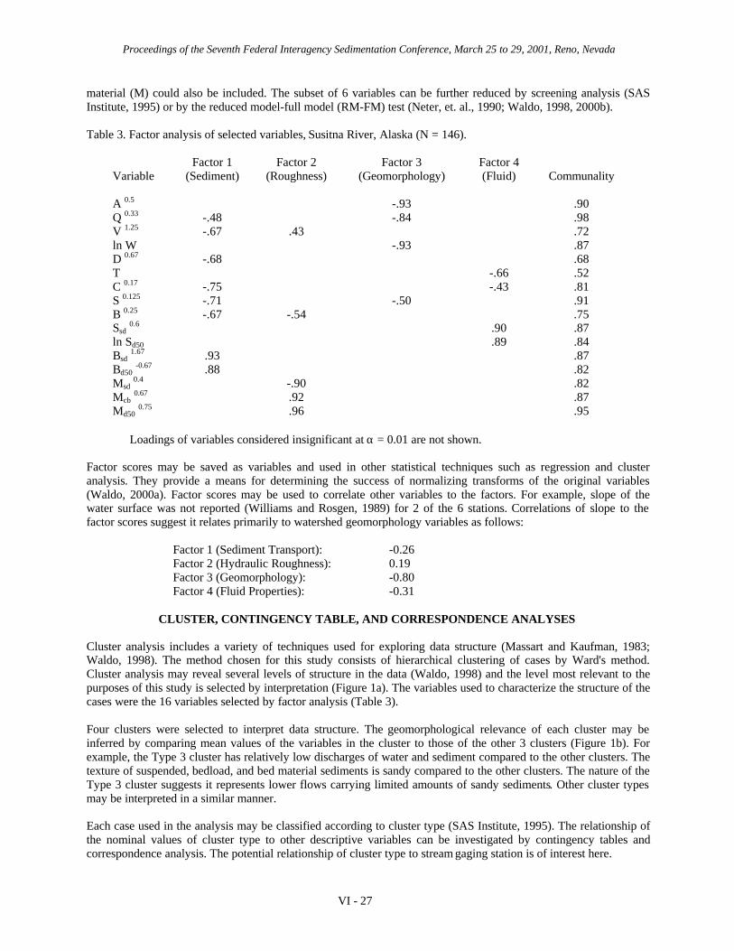
Proceedings of the Seventh Federal Interagency Sedimentation Conference, March 25 to 29, 2001, Reno, Nevada
VI - 27
material (M) could also be included. The subset of 6 variables can be further reduced by screening analysis (SASInstitute, 1995) or by the reduced model-full model (RM-FM) test (Neter, et. al., 1990; Waldo, 1998, 2000b).
Table 3. Factor analysis of selected variables, Susitna River, Alaska (N = 146).
Factor 1 Factor 2 Factor 3 Factor 4Variable (Sediment) (Roughness) (Geomorphology) (Fluid) Communality
A 0.5 -.93 .90Q 0.33 -.48 -.84 .98V 1.25 -.67 .43 .72ln W -.93 .87D 0.67 -.68 .68T -.66 .52C 0.17 -.75 -.43 .81S 0.125 -.71 -.50 .91B 0.25 -.67 -.54 .75Ssd 0.6 .90 .87ln Sd50 .89 .84Bsd 1.67 .93 .87Bd50 -0.67 .88 .82Msd 0.4 -.90 .82Mcb 0.67 .92 .87Md50 0.75 .96 .95
Loadings of variables considered insignificant at α = 0.01 are not shown.
Factor scores may be saved as variables and used in other statistical techniques such as regression and clusteranalysis. They provide a means for determining the success of normalizing transforms of the original variables(Waldo, 2000a). Factor scores may be used to correlate other variables to the factors. For example, slope of thewater surface was not reported (Williams and Rosgen, 1989) for 2 of the 6 stations. Correlations of slope to thefactor scores suggest it relates primarily to watershed geomorphology variables as follows:
Factor 1 (Sediment Transport): -0.26Factor 2 (Hydraulic Roughness): 0.19Factor 3 (Geomorphology): -0.80Factor 4 (Fluid Properties): -0.31
CLUSTER, CONTINGENCY TABLE, AND CORRESPONDENCE ANALYSES
Cluster analysis includes a variety of techniques used for exploring data structure (Massart and Kaufman, 1983;Waldo, 1998). The method chosen for this study consists of hierarchical clustering of cases by Ward's method.Cluster analysis may reveal several levels of structure in the data (Waldo, 1998) and the level most relevant to thepurposes of this study is selected by interpretation (Figure 1a). The variables used to characterize the structure of thecases were the 16 variables selected by factor analysis (Table 3).
Four clusters were selected to interpret data structure. The geomorphological relevance of each cluster may beinferred by comparing mean values of the variables in the cluster to those of the other 3 clusters (Figure 1b). Forexample, the Type 3 cluster has relatively low discharges of water and sediment compared to the other clusters. Thetexture of suspended, bedload, and bed material sediments is sandy compared to the other clusters. The nature of theType 3 cluster suggests it represents lower flows carrying limited amounts of sandy sediments. Other cluster typesmay be interpreted in a similar manner.
Each case used in the analysis may be classified according to cluster type (SAS Institute, 1995). The relationship ofthe nominal values of cluster type to other descriptive variables can be investigated by contingency tables andcorrespondence analysis. The potential relationship of cluster type to stream gaging station is of interest here.

Proceedings of the Seventh Federal Interagency Sedimentation Conference, March 25 to 29, 2001, Reno, Nevada
VI - 28
Contingency table analysis produces a statistic known as the uniformity coefficient, R2(U), that indicates the degreeof association between two descriptive variables. The value of R2(U) = 0.70 (Figure 2a) indicates a high degree ofassociation between cluster type and gaging station. Correspondence analysis shows which stations associate morestrongly with which cluster type (Figure 2b).
The 6 stations may be grouped into 4 classes depending on their correspondence to cluster type (Table 1). Thisassociates cluster type, originally determined from 165 cases, with all 187 cases. Missing values of underrepresentedvariables (e.g., water surface slope) can be predicted by computing means or medians of the variables for eachcluster type or correspondence class. Either cluster type or correspondence class may be used to define indicatorvariables for use in regression analysis. The significance of differences between types or stations in various modelspaces can be assessed by statistical hypothesis tests.
REGRESSION ANALYSIS
Regression analysis is typically used in sediment transport studies for calibrating predictive models. Suspendedsediment and bedload discharges are regressed on water discharge or other predictors. Calibrations are performedseparately at each station (Knott, et. al., 1987). When data are sparse at certain stations (e.g., Susitna River atChulitna River and Yentna River, Table 4) the significance of calibrations is suspect because of low statistical power(Waldo, 2000b).
An alternative strategy consists of using regression in the data mining approach. Select the dependent variables forwhich predictive models are to be developed (e.g., suspended sediment and bedload discharges). Assure that thosevariables are included in the factor and cluster analysis steps of the data mining procedure. Select candidatepredictor variables from factor analysis. Use the results of cluster and correspondence analysis to define convenientyet meaningful groups. Include indicator variables representing the descriptive groups in the predictor set.Appropriate indicator variables and their interactions with the continuous predictors can significantly increase R2
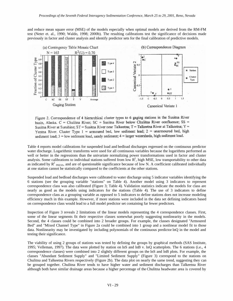
Proceedings of the Seventh Federal Interagency Sedimentation Conference, March 25 to 29, 2001, Reno, Nevada
VI - 29
and reduce mean square error (MSE) of the models especially when optimal models are derived from the RM-FMtest (Neter et. al., 1990; Waldo, 1998; 2000b). The resulting calibrations test the significance of decisions madepreviously in factor and cluster analysis and identify predictor sets for the final calibration of predictive models.
Table 4 reports model calibrations for suspended load and bedload discharges regressed on the continuous predictorwater discharge. Logarithmic transforms were used for all continuous variables because the logarithms performed aswell or better in the regressions than the univariate normalizing power transformations used in factor and clusteranalysis. Some calibrations to individual stations suffered from low R2, high MSE, low transportability to other dataas indicated by R2 PRESS, and are of questionable significance because of low N. A coefficient calibrated individuallyat one station cannot be statistically compared to the coefficients at the other stations.
Suspended load and bedload discharges were calibrated to water discharge using 5 indicator variables identifying the6 stations (see the grouping variable "stations" on Table 4). Another model using 3 indicators to representcorrespondence class was also calibrated (Figure 3; Table 4). Validation statistics indicate the models for class arenearly as good as the models using indicators for the stations (Table 4). The use of 3 indicators to definecorrespondence class as a grouping variable as opposed to 5 indicators to define stations does not increase modelingefficiency much in this example. However, if more stations were included in the data set defining indicators basedon correspondence class would lead to a full model predictor set containing far fewer predictors.
Inspection of Figure 3 reveals 2 limitations of the linear models representing the 4 correspondence classes. First,some of the linear segments fit their respective classes somewhat poorly suggesting nonlinearity in the models.Second, the 4 classes could be combined into 2 broader groups. For example, the classes designated "ArmouredBed" and "Mixed Channel Type" in Figure 2a could be combined into 1 group and a nonlinear model fit to thosedata. Nonlinearity may be investigated by including polynomials of the continuous predictor lnQ in the model andtesting their significance.
The viability of using 2 groups of stations was tested by defining the groups by graphical methods (SAS Institute,1995; Velleman, 1997). The data were plotted by station on lnS and lnB v. lnQ scatterplots. The 6 stations (i.e., 4correspondence classes) were combined into 2 slightly different groups on the lnS and lnB plots. For example, theclasses "Abundant Sediment Supply" and "Limited Sediment Supply" (Figure 3) correspond to the stations onChulitna and Talkeetna Rivers respectively (Figure 2b). The data plot on nearly the same trend, suggesting they canbe grouped together. Chulitna River tends to have higher water and sediment discharges than Talkeetna Riveralthough both have similar drainage areas because a higher percentage of the Chulitna headwater area is covered by

Proceedings of the Seventh Federal Interagency Sedimentation Conference, March 25 to 29, 2001, Reno, Nevada
VI - 30
glaciers (Table 1; Knott et al. 1987). The two visual groups seem to highlight differences in sediment transportbetween stations on tributaries and stations on the main stem of the Susitna River.
Table 4. Model calibrations, Susitna River, Alaska.
GroupingVariable N p R2 MSE R2 PRESS p--value
Suspended Load
C 43 1 .913 .098 .900 <.0001SC 11 1 .752 .427 .628 .0005SS 42 1 .869 .141 .854 <.0001ST 39 1 .900 .188 .886 <.0001T 42 1 .860 .275 .846 <.0001Y 10 1 .810 .121 .719 .0004
Stations 187 7 .924 .182 .917 <.0001Class1 187 5 .922 .186 .916 <.0001
Bedload
C 43 1 .154 .230 .055 .0094SC 11 1 .310 .457 --2 .0753SS 42 1 .185 .405 .119 .0045ST 39 1 .754 .294 .716 <.0001T 42 1 .519 .556 .460 <.0001Y 10 1 .012 .124 --2 .7659
Stations 187 7 .830 .363 .812 <.0001Class1 187 6 .799 .427 .780 <.0001
N = number of observations; p = number of predictors; R2 = coefficient of determination; MSE = mean square error;R2
PRESS = R2 computed from Press statistic; p-value from ANOVA table for the regression.
1 Class determined by correspondence of 6 stations to 4 cluster types. 2 R2PRESS is undefined because Press statistic
> total sum of squares.
Regression analysis and the RM-FM test are useful for screening the significance of continuous predictors other thanQ. Selections of candidate predictors were made by factor analysis. Models for lnS and lnB were obtained using anindicator based on the 2 groups identified by the visual method. Suspended sediment was found to be sensitive tolnD in addition to lnQ and Md50 enhanced the calibration of the bedload model. Polynomial terms of the continuouspredictors and their interactions with the indicator variable and each other were included in the full models. Thisresulted in linear models, an assumption important to least squares regression (Figure 4). The suspended sedimentmodel has normally distributed residuals with constant variance but exhibit a significant degree of dependence(Figure 4a). The bedload model has normally distributed independent residuals but with nonconstant variance(Figure 4b). This suggests the type of generalized least squares to use in the final calibrations of the models:correction of serial correlation of the suspended sediment model and weighted least squares to correct nonconstantvariance in the bedload model.
CONCLUSIONS
1. Data mining leads to a sophisticated understanding of data structure. Knowledge of data structure improvestheoretical understanding of the data and enables calibration of reliable predictive models. The data miningmethodology enables efficient use of existing data in addressing specific problems (e.g., sediment transport

Proceedings of the Seventh Federal Interagency Sedimentation Conference, March 25 to 29, 2001, Reno, Nevada
VI - 31

Proceedings of the Seventh Federal Interagency Sedimentation Conference, March 25 to 29, 2001, Reno, Nevada
VI - 32
predictions). This approach might be used in the development of data collecting strategies to optimize results offuture experiments.
2. Factor analysis finds meaningful groups of continuous variables, reduces the number of variables needed insubsequent analyses, suggests candidates to include in regression predictor sets, and produces factor scoresuseful for validating other statistical procedures.
3. Cluster analysis and graphical methods define groups of cases that can be interpreted in a manner that increasesunderstanding of the data structure. Indicator variables may be defined on the basis of cluster type and tested forsignificance by regression analysis.
4. Contingency tables and correspondence analysis relate cluster types to gaging stations. This enhancesunderstanding and interpretation of the data structure and facilitates model calibration.
5. Regression analysis with the RM-FM test evaluates hypotheses about the data structure, investigates potentialpredictor sets for model calibration, and suggests methods needed to calibrate the final model as efficiently andaccurately as possible.
6. The data structure reflects geomorphic attributes of the Susitna River basin as well as hydraulic andsedimentologic relationships. Data mining methods enable incorporation of that information into modelcalibrations through the use of indicator variables and the process of identifying key predictor variables.
REFERENCES
Brabets, T.P., 1996, Evaluation of the streamflow-gaging network of Alaska in providing regional streamflowinformation, Water-resources investigation report 96-4001, USGS, Anchorage, Alaska.
Knott, J. M., Lipscomb, S. W., Lewis, T. W., 1987, Sediment transport characteristics of selected streams in theSusitna River basin, Alaska: Data for water year 1985 and trends in bedload discharge, 1981-85, USGS open-file report.
Massart, D. L., Kaufman, L., 1983, The interpretation of analytical chemical data by the use of cluster analysis, JohnWiley and Sons, New York.
Neter, J., Wasserman, W., Kutner, M. H., 1990, Applied linear statistical models, Irwin, Boston.
SAS Institute, 1995, JMP statistics and graphics guide, SAS Institute, Cary, North Carolina.
Stevens, J., 1992, Applied multivariate statistics for the social sciences, Lawrence Erlbaum, Hillsdale, New Jersey.
Velleman, P. F., 1997, Data desk version 6.0 statistics guide, Data Description Inc., New York.
Waldo, P. G., 1998, Prediction of sealing capacity of faults: a pilot study using observational statistics, Ph.D.dissertation, Univ. Tex. at Arlington, Arlington, Texas.
Waldo, P. G., 2000a, Factor analysis and hydrologic data from Texas, manuscript in preparation.
Waldo, P. G., 2000b, Selecting optimal regression models by the reduced model-full model test, manuscript inpreparation.
Williams, G. P., Rosgen, D. L., 1989, Measured total sediment loads (suspended loads and bedloads) for 93 UnitedStates streams, USGS open-file report.

Proceedings of the Seventh Federal Interagency Sedimentation Conference, March 25 to 29, 2001, Reno, Nevada
VI - 33
A Probabilistic Approach To Modeling Erosion for Spatially-Varied Conditions
W. J. Elliot P. R. Robichaud C. D. PannkukProject Leader Research Engineer Soil Scientist
USDA-FOREST SERVICE, ROCKY MOUNTAIN RESEARCH STATIONMoscow, ID 83843
Mailing address: 1221 South Main, Moscow, ID 83843; Tel. 208 882 3557; email [email protected]
INTRODUCTION
Soil erosion by water is a complex process resulting from the interactions among a number offactors including weather patterns, soil properties, topography, and the influences of surfacevegetation. Natural variability is a dominant characteristic of each of these factors, which makespredicting soil erosion rates difficult. In many forest conditions, and some rangeland conditions,erosion may be minimal under vegetated conditions unless the site is disturbed. Disturbancesmay be fire, logging, grazing, or severe precipitation events. The most extreme erosion ratesoccur when severe weather follows a major disturbance, particularly a severe wildfire.
Natural resource managers need tools to aid in predicting soil erosion following wildfires toestimate potential loss of onsite productivity, or potential offsite damage from sediment toaquatic ecosystems or other beneficial uses dependent on quality water. Current erosionprediction tools generally are developed from agricultural erosion models, which are intended toprovide long-term estimates of soil erosion rather than evaluate short-term risks. These modelstypically provide an “average” erosion value, and do not give any estimate of the likelihood ofmajor upland erosion occurring.
Process-based erosion models may provide a means for evaluating complex distributions ofdisturbance from a range of possible weather sequences, but the effort to parameterize suchmodels makes them unsuitable for widespread application. However, they can play a role inassisting researchers to analyze some of the interactions between erosion factors.
We are developing an interface to aid in the analysis of erosion prediction following fire, or asimilar major disturbance, in forests and rangelands. This paper addresses how we intend toincorporate the inherent variability associated with the predicted erosion rate, and how thatvariability is influenced by weather, spatial distribution of disturbances, and soil properties.
POST-FIRE EROSION FACTORS
Hillsides are more susceptible to erosion following a fire with decreased canopy and surfaceresidue, and in some case a soil that is water repellent. Water repellency is a process that occurswhen volatilized hydrocarbons released by the fire condense and coat soil particles andaggregates. These hydrocarbons repel water, which reduces infiltration rates and increasesrunoff, erosion and sediment delivery from hillsides. With time, they are dissolved by

Proceedings of the Seventh Federal Interagency Sedimentation Conference, March 25 to 29, 2001, Reno, Nevada
VI - 34
infiltrating water from rainfall and snowmelt. The reduction in vegetative canopy and surfaceresidue dramatically increases the potential for soil erosion by increasing the area susceptible toraindrop impact and decreasing the potential for sediment deposition. In the year following afire, vegetation regrowth can be rapid because of increased availability of soil nutrients, anddecreased competition for sunlight and soil water by large trees. Hence, a burned site has a fargreater likelihood of erosion the year following a fire, with the risk dropping rapidly asvegetation regrows, residue accumulates, and water-repellent chemicals break down and areflushed from or translocated in the soil.
VARIABILITY IN SOIL EROSION
Variability has been identified as a dominant feature in soil erosion research. Coefficients ofvariations and confidence intervals are the most familiar ways of reporting uncertainty, buttypically they are used only for comparisons. The concept of confidence intervals can beextended to a complete probability distribution, which can describe a range of values, each valuewith an associated probability of occurrence.
Weather Weather is highly variable from one year to the next. Years with a wet spring,encouraging considerable vegetation growth, followed by a prolonged, hot summer are morelikely to have severe rangeland wild fires than are years with drier springs, or cooler or wettersummers. In forests, low snow pack years with hot dry springs and summers are more likely tohave severe wild fires.
Following a fire, if the weather is very dry, there will be little natural or seeded vegetationregrowth and little soil recovery from water repellent conditions. This means that the site canremain susceptible to erosion for another season. If the weather is very wet, and the soils arewater repellent, there is a high likelihood of severe soil erosion, but also there will be rapidvegetation recovery. Runoff from rainfall or rain-on-snow events will be much greater thanrunoff from melting snow. Generally, snowmelt rates are 1 to 2 mm hr-1, whereas rainfall ratesup to 25 mm hr-1 are common.
Once a site has recovered, rainfall rates in excess of 50 mm hr-1 or total rainfall amounts greaterthan 100 mm within a day or two are necessary before any significant upland erosion will occur.This seldom happens in many forested areas.
Fire Fire effects on erosion are not homogenous. Fire severity is a description of the impact of afire on the soil and its litter layer. The severity of a fire varies widely in space, depending onfuel load, moisture conditions and weather at the time of fire, and the topography. Thisvariability often creates variability in severity, leading to mosaic landscapes. Areas that aredrier, such as those near ridge tops, and areas with greater amounts of fuel, may experiencehigher severity fires. Areas that are wetter, such as riparian areas, will likely have less severefires (Robichaud and Miller 2000).
Soil and Spatial Variability Soil properties are naturally highly variable. Soil erosionexperiments generally measure standard deviations in erodibility values similar to the means, and

Proceedings of the Seventh Federal Interagency Sedimentation Conference, March 25 to 29, 2001, Reno, Nevada
VI - 35
coefficients of variation greater than 30 percent are common (Elliot et al. 1989). Soils near thetops of ridges tend to be coarser grained and shallower, whereas soils at the bottoms of hillslopes may be finer grained, while flood plains vary widely depending on past geomorphicprocesses. After fires, this variability increases with variability in water repellency.
The combined effects of a mosaic in fire severity and soil variability result in spatial variabilityof soil erodibility that has some degree of predictability, but a great deal of natural variability.Spatial variability analyses have shown that following some fires, there are definite trends indegree of fire severity, whereas, the variability is evenly distributed on a hillslope or watershedfollowing other fires (Robichaud and Miller 2000).
COMBINING VARIABILITIES
To understand the combined variabilities of climate, fire severity, and soil properties, numerousanalyses are carried out combining various storms or weather patterns, different distributions ofdisturbance, and an array of soil properties that occur for a given severity of fire. It isunreasonable to expect that a single estimate of soil erosion will capture the combinedprobabilities. A better estimate of erosion is to provide a range of possible erosion predictionsusing a Monte-Carlo approach (Haan 1994). The estimated erosion rate can then be expressed asthe probability of a given level of erosion being exceeded. One of the challenges for this type ofmodeling is developing the statistical distributions of the dependent variables.
THE WEPP MODEL
We chose to use the Water Erosion Prediction Project (WEPP) model as the driver for theproposed model. WEPP is a physically-based soil erosion model that describes the processesthat cause erosion (Laflen et al. 1997). As long as the processes are correctly described, and thedetails of the site conditions can be described by the input variables, then the model can beapplied. For some runs, WEPP may require up to 400 input variables describing soil andvegetative properties in great detail. Packaged with WEPP is a daily weather generator,CLIGEN. CLIGEN stochastically generates daily weather sequences, which include theoccurrence of precipitation, and the amount and duration of precipitation on a wet day (Nicks etal. 1995).
The WEPP model can be run either for single storms, with initial conditions such as soil watercontent, surface cover and soil erodibility specified for the storm, or in continuous mode wherethese values are automatically altered daily for a number of years of daily weather. Outputoptions from WEPP include average annual runoff and erosion rates, annual erosion rates for thelength of run, or event runoff and erosion rates for every runoff event during the period ofsimulation (Flanagan and Livingston 1995). The WEPP model has been applied to forestconditions with reasonable results, and the database to support the model is increasing (Elliot andHall 1997).
PROPOSED SPATIALLY-VARIED MODEL
We are developing a soil erosion interface to use with the WEPP model, combined with a

Proceedings of the Seventh Federal Interagency Sedimentation Conference, March 25 to 29, 2001, Reno, Nevada
VI - 36
stochastic input data set, to estimate the probability of a given level of soil erosion (Robichaud etal. 2000). The user will provide inputs related to local climate, degree of fire severity, soiltexture, and topography. The user will be given the option to use a storm generated by theinterface, or to specify the desired storm amount and duration. Once the storm is selected, theproposed interface will be run for a large number of spatial distributions and soil propertycombinations, producing a range of possible soil erosion rates. The results will be presented tothe user in either a tabular or a graphical format.
Climate There are few weather stations in remote forested areas, a weather station somedistance from the site of concern may not provide an adequate estimate for a storm. TheCLIGEN weather generator has a database of over 1100 stations (Flanagan and Livingston1995). We have expanded that database to over 2600 (Scheele et al. 2001). In addition, we haveaccess to the PRISM database that contains monthly precipitation values for a 4 km gridcovering the entire continental U.S. This grid will aid users to select a local climate for theCLIGEN weather generator (Scheele et al. 2001). CLIGEN can then generate a long termclimate for running WEPP. To estimate the risk of a given size of storm, a 100-year climate filewill be generated to run WEPP. WEPP will be run and the output for each event will berequested. The event output file will be sorted to determine the greatest, second greatest, fifth,tenth, and twentieth greatest erosion events. The storms for these events will provide the userwith a choice of 5-, 10-, 20-, 50-, and 100-year return periods for storms. The user can select thedesired return period storm, or specify a storm.
Soil Research has shown that it is not possible to statistically differentiate more than two levelsof fire severity, which we define as low and high (Robichaud et al. 1993). The most importanterosion prediction parameters affected by fire severity include percent ground cover, saturatedhydraulic conductivity, and rill erodibility. Table 1 presents the range of values that have beenmeasured in field studies. These values can be adjusted for different textures based on researchobservations (Robichaud 2000).
Spatial Spatial variability can be described with different distributions of severity on thelandscape (figure 1). Figure 1 shows that the distributions can be grouped into categories oferosion risk. Most managers prefer to describe burned sites by these categories of erosion risk as“High”, “Moderate” or “Low”. In a previous study, Robichaud and Monroe (1997) showed thatdividing the hill into three elements is adequate to describe the range of variation of surfaceerosion as influenced by spatial variation.
RESULTS
Climate Variability Table 2 presents the results of a set of WEPP runs comparing differentstorm events for a forest with a moderate erosion risk fire. Note that the events that experienced
Table 1. Range of erodibility values observed in field studies.FireSeverity
Remaining GroundCover (percent)
Saturated hydraulicconductivity (mm hr-1)
Rill erodibility(s m-1)
Low 40 – 100 12 – 30 3 x 10⁻⁵ – 3 x 10⁻⁴
High 0 – 60 6 – 15 2.5 x 10⁻⁴ – 2.5 x 10⁻³
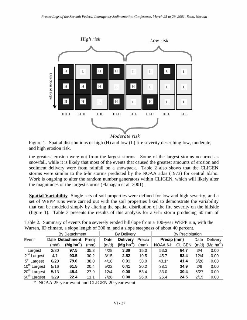
Proceedings of the Seventh Federal Interagency Sedimentation Conference, March 25 to 29, 2001, Reno, Nevada
VI - 37
the greatest erosion were not from the largest storms. Some of the largest storms occurred assnowfall, while it is likely that most of the events that caused the greatest amounts of erosion andsediment delivery were from rainfall on a snowpack. Table 2 also shows that the CLIGENstorms were similar to the 6-hr storms predicted by the NOAA atlas (1973) for central Idaho.Work is ongoing to alter the random number generators within CLIGEN, which will likely alterthe magnitudes of the largest storms (Flanagan et al. 2001).
Spatial Variability Single sets of soil properties were defined for low and high severity, and aset of WEPP runs were carried out with the soil properties fixed to demonstrate the variabilitythat can be modeled simply by altering the spatial distribution of the fire severity on the hillside(figure 1). Table 3 presents the results of this analysis for a 6-hr storm producing 60 mm of
H
L
LH
L
L
H
L
L
L
L
L
H
L
H
H
L
H
H
L
H
H
H
H
High risk
Moderate risk
Low risk
HHH LHH HHL HLH LHL LLH HLL LLL
Direction of slope
Figure 1. Spatial distributions of high (H) and low (L) fire severity describing low, moderate,and high erosion risk.
Table 2. Summary of events for a severely eroded hillslope from a 100-year WEPP run, with theWarren, ID climate, a slope length of 300 m, and a slope steepness of about 40 percent.
By Detachment By Delivery By PrecipitationEvent Date Detachment Precip Date Delivery Precip Precip (mm) Date Delivery
(m/d) (Mg ha-1) (mm) (m/d) (Mg ha-1) (mm) NOAA 6-h CLIGEN (m/d) (Mg ha-1)Largest 3/30 97.5 35.3 4/28 3.39 15.0 53.3 64.7 3/4 0.00
2nd Largest 4/1 93.5 30.2 3/15 2.52 19.5 45.7 53.4 12/4 0.005th Largest 6/20 79.0 38.0 4/18 0.91 38.0 43.1* 41.4 6/26 0.0010th Largest 5/16 61.5 20.4 5/22 0.41 30.2 38.1 34.9 2/9 0.0020th Largest 5/13 45.4 27.9 12/4 0.00 53.4 33.0 30.4 6/27 0.0050th Largest 3/29 22.4 11.1 7/28 0.00 26.0 25.4 24.5 2/15 0.00
* NOAA 25-year event and CLIGEN 20-year event

Proceedings of the Seventh Federal Interagency Sedimentation Conference, March 25 to 29, 2001, Reno, Nevada
VI - 38
precipitation. A 60-mm rainfall event is about a 100-year event based on CLIGEN and theNOAA maps (table 2). Table 3 is ordered by upland erosion rates, and apparently the order is
not the same for erosion as it is for sediment yield. A reasonable conclusion from this table isthat the range of soil erosion rates due to spatial variability only is 55 to 77 Mg ha-1 for a highrisk fire, 38 to 57 Mg ha-1 for a moderate risk fire, and 5 to 45 Mg ha-1 for a low risk fire from a60-mm precipitation event.
Soil Variability Soil properties were varied over the range of values for low and high severityconditions presented in Table 1, for a 100-m long, 40 percent slope hill, with a 60-mm, 6-hrstorm. Figure 2 shows the results of these runs, with low severity predicted erosion rates varyingfrom 0.06 to 3.8 Mg ha-1, and high severity rates from 2.3 to 25.8 Mg ha-1 for a 60-mm 6-hstorm. Note that the range of predicted erosion rates is greater than two magnitudes. As acomparison, observed erosion rates from a 13-mm storm following the spring after a highseverity fire were zero and 0.19 Mg ha-1 in a study in progress in the Wenatchee National Forestin Central Washington, and annual totals were zero and 4.4 Mg ha-1 on a 30 percent slope for twoadjacent plots in the Wallowa-Whitman National Forest in Eastern Oregon the first year after asevere fire. Figure 2 also shows that there is an overlap in the distributions of both runoff and
Table 3. Effects of the different spatial arrangements on runoff, hillside erosion, and sedimentdelivery for single sets of low and high severity soil properties. The table is in descendingorder by erosion rate.
Erosion Risk Distribution Runoff (mm) Erosion (Mg ha-1) Sed Yield (Mg ha-1)High HHH 22.7 77.0 73.0High LHH 20.9 66.2 61.5High & Mod HHL 17.2 56.8 30.7High & Mod HLH 17.5 54.5 52.1Mod & Low LHL 14.6 44.5 25.1Mod & Low LLH 14.9 38.4 36.7 Low HLL 14.4 14.5 13.6 Low LLL 11.9 4.6 4.4
0 5 10 15 20 25 30
Low severity runoff
High severity runoff
Low severity erosion
High severity erosion
Runoff (mm) or Erosion Rate (Mg/ha)
Figure 2. Effects of fire severity on predicted ranges of runoff and soil erosion for a 100-m long,40 percent slope hill, with a 60-mm, 6-hr storm.

Proceedings of the Seventh Federal Interagency Sedimentation Conference, March 25 to 29, 2001, Reno, Nevada
VI - 39
erosion rates between high and low severity.
DISCUSSION
The results that are presented as a range in figure 2 can also be presented as exceedance values(figure 3). One of the challenges for the proposed application is that by selecting a design storm,the user has already limited predicted erosion to a very small set of storms. The results presentedin figure 3 are associated with a 100-year precipitation event. Figure 3 shows that there is a tenpercent chance in the year following a fire that erosion will exceed 26 Mg ha-1 storm, and a 90percent chance that runoff will be less than 16 mm and erosion less than 26 Mg ha-1 from a 100year storm event.
INTERFACES
To incorporate climate variability, spatial variability, and soil variability into erosion predictionis complex and time consuming with the current erosion models, including WEPP. Currentmodels do not incorporate the ability to carry out return period analysis of storms. For eachspatial arrangement and each soil condition a separate run or calculation is required. We arecurrently developing an interface that will allow the user to select or specify a storm, a soiltextural category, a level of erosion risk, and slope length and steepness. The interface will thencarry out several hundred computer runs for the given level of fire risk, and present the user witha table or graph such as that in figure 3, interpreting the results of the likelihood of soil erosionexceeding a given amount (Robichaud et al. 2000).
SUMMARY
Variability is a dominant factor in soil erosion prediction on forest landscapes. Variables includeclimate, soil properties, and the spatial distribution of fire severity. The range of erosion ratescan vary by over a magnitude due to spatial variability, and over two magnitudes due to soilvariability. A computer tool is under development to aid managers in evaluating the runoff anderosion risks associated with wildfire for a given storm.
0
5
10
15
20
25
30
0 10 20 30 40 50 60 70 80 90 100
Exceedance Probability
Ru
no
ff (
mm
) o
r E
rosi
on
(M
g/h
a)
Runoff
Erosion
Figure 3. Example of output from the proposed fire risk interface.

Proceedings of the Seventh Federal Interagency Sedimentation Conference, March 25 to 29, 2001, Reno, Nevada
VI - 40
REFERENCES
Elliot, W. J., Liebenow, A. M., Laflen, J. M., Kohl, K. D., 1989, A compendium of soil erodibility datafrom WEPP cropland soil field erodibility experiments 1987 & 88. NSERL Report No. 3.Columbus, OH: The Ohio State University, and W. Lafayette, IN: USDA Agricultural ResearchService, 319 p.
Elliot, W. J., Hall, D. E., 1997, Water Erosion Prediction Project (WEPP) forest applications. GeneralTechnical Report INT-GTR-365. Ogden, UT: USDA Forest Service, Rocky Mountain ResearchStation, 11 p.
Flanagan, D. C., Livingston, S. J. (eds.), 1995, WEPP User Summary. NSERL Report No. 11, W.Lafayette, IN: National Soil Erosion Research Laboratory, 131 p.
Flanagan, D. C., Meyer, C. R., Yu, B., Scheele, D. L., 2001, Evaluation and enhancement of the CLIGENweather generator. Proceedings of the ASAE International Symposium on Soil Erosion Researchfor the 21st Century. Honolulu, HI. Jan. 3-5, 2001. St. Joseph, MI: ASAE, 4 p.
Haan, C. T., 1994, Statistical Methods in Hydrology. Ames, IA: Iowa State University Press, 378 p.
Laflen, J. M., Elliot, W. J., Flanagan, D. C., Meyer, C. R., Nearing, M. A., 1997, WEPP–Predicting watererosion using a process-based model. Journal of Soil and Water Conservation 52(2), 96-102.
National Oceanic and Atmospheric Admin. (NOAA), 1973, NOAA Atlas 2, Volume V – Idaho.Precipitation-frequency Atlas of the Western United States, Available online at<http://www.wrcc.dri.edu/pcpnfreq.html>.
Nicks, A. D., Lane, L. J., Gander, G. A., 1995, Chapter 2. Weather Generator. In Flanagan, D. C.,Nearing, M. A., USDA-Water Erosion Prediction Project Hillslope Profile and Watershed ModelDocumentation. W. Lafayette, IN: USDA Agricultural Research Service, 2.1-2.22.
Robichaud, P. R., 2000, Fire effects on infiltration rates after prescribed fire in Northern Rocky Mountainforests, USA. Journal of Hydrology 231-232, 220-229.
Robichaud, P. R., Luce, C. H., Brown, R. E., 1993, Variation among different surface conditions intimber harvest sites in the Southern Appalachians. International Workshop on Soil Erosion,Proceedings. Moscow, Russia. West Lafayette, IN: The Center for Technology Transfer andPollution Prevention, Purdue University, 231-241.
Robichaud, P. R., Miller, S. M., 2000, Spatial interpolation and simulation of post-burn duff thicknessafter prescribed fire. Accepted for publication in the International Journal of Wildland Fire.
Robichaud, P. R., Monroe, T. M., 1997, Spatially-varied erosion modeling using WEPP for timberharvested and burned hillslopes. Presented at the 1997 ASAE International Meeting, Minneapolis,MN. August 10-14. Paper No. 975015. St. Joseph, MI: ASAE, 8 p.
Robichaud, P. R., Elliot, W. J., Pierson, F. B., Wohlgemuth, P. M., 2000, Risk assessment of fuelmanagement practices on hillslope erosion processes. In Neuenschwander, L. F., Ryan, K. C.,(technical eds.) Proceedings from the Joint Fire Science Conference and Workshop. June 15-17,1999. Boise, ID. Moscow, ID: University of Idaho 58-65.
Scheele, D. L., Elliot, W. J., Hall, D. E., 2001, Enhancements to the CLIGEN weather generator formountainous terrain. Proceedings of the ASAE International Symposium on Soil Erosion Researchfor the 21st Century. Honolulu, HI. Jan. 3-5, 2001. St. Joseph, MI: ASAE, 4 p.

Proceedings of the Seventh Federal Interagency Sedimentation Conference, March 25 to 29, 2001, Reno, Nevada
VI - 41
SEDIMENT LABORATORY QUALITY-ASSURANCE PROJECT:STUDIES ON METHODS AND MATERIALS
By J. D. Gordon, Hydrologist, U.S. Geological Survey, Denver, Colorado; C.A. Newland, Physical Scientist,ATA Services, Inc., Denver, Colorado; and J.R. Gray, Hydrologist, U.S. Geological Survey, Reston, Virginia
Abstract: In August 1996 the U.S. Geological Survey initiated the Sediment Laboratory Quality-Assurance project.The Sediment Laboratory Quality Assurance project is part of the National Sediment Laboratory Quality-Assuranceprogram. This paper addresses the findings of the sand/fine separation analysis completed for the single-blindreference sediment-sample project and differences in reported results between two different analytical procedures.
From the results it is evident that an incomplete separation of fine- and sand-size material commonly occursresulting in the classification of some of the fine-size material as sand-size material. Electron microscopy analysissupported the hypothesis that the negative bias for fine-size material and the positive bias for sand-size material islargely due to aggregation of some of the fine-size material into sand-size particles and adherence of fine-sizematerial to the sand-size grains. Electron microscopy analysis showed that preserved river water, which was low indissolved solids, specific conductance, and neutral pH, showed less aggregation and adhesion than preserved riverwater that was higher in dissolved solids and specific conductance with a basic pH. Bacteria were also foundgrowing in the matrix, which may enhance fine-size material aggregation through their adhesive properties.
Differences between sediment-analysis methods were also investigated as part of this study. Suspended-sedimentconcentration results obtained from one participating laboratory that used a total-suspended solids (TSS) method hadgreater variability and larger negative biases than results obtained when this laboratory used a suspended-sedimentconcentration method. When TSS methods were used to analyze the reference samples, the median suspended-sediment concentration percent difference was –18.04 percent. When the laboratory used a suspended-sedimentconcentration method, the median suspended-sediment concentration percent difference was –2.74 percent. Thepercent difference was calculated as follows:
Percent difference = reported mass - known mass known mass
X 100 .( )INTRODUCTION
The collection and analysis of fluvial sediment samples has been an integral part of hydrologic studies in the UnitedStates for over 100 years (Glysson, 1989). To support this sediment monitoring and research, the U.S. GeologicalSurvey (USGS) operates laboratories for the analysis of the physical characteristics of sediment.
Working with the USGS Sediment Action Committee and the USGS Water Quality Service Unit in Ocala, Florida,the Branch of Quality Systems (BQS) distributed test samples as part of a pilot standard reference study in 1992 and1994 (George and Schroder, 1996). Results of the pilot studies indicated that a standard reference-sample projectwas feasible and practical. Following the 1992 and 1994 pilot studies, the BQS continued to pursue the developmentand testing of a standard reference-sample project for measurement of physical sediment properties. In 1996, theseefforts led to an external quality-assurance project to ensure that the physical sediment data produced or used by theUSGS are of a known quality and are sufficient to provide long-term comparability and consistency. The SedimentLaboratory Quality-Assurance (SLQA) project began in August 1996 and is part of the National SedimentLaboratory Quality-Assurance (NSLQA) program. The NSLQA program focuses on all quantitative analyses doneon water-sediment mixtures to derive concentrations and sand/fine separations. The program is composed of sevencomponents: (1) a single-blind reference sediment-sample project, (2) a double-blind reference sediment-sampleproject, (3) data analysis and reporting for each laboratory on a national basis, (4) follow-up evaluations, (5) onsitelaboratory evaluations, (6) documentation of laboratory quality-assurance plans and quality-control procedures, and(7) training in laboratory operational procedures. The SLQA project contains the first four parts of the NSLQAprogram and is intended to provide quantitative information on sediment-data quality to sediment-laboratorycustomers (U.S. Geological Survey Office of Surface Water Technical Memorandum No. 98.05, 1998).

Proceedings of the Seventh Federal Interagency Sedimentation Conference, March 25 to 29, 2001, Reno, Nevada
VI - 42
Between August 1996 and September 1999, the BQS completed eight single-blind sediment laboratoryintercomparison studies. In each study, a set of nine single-blind reference samples were sent to each participatinglaboratory for analysis of suspended-sediment concentration, sediment mass, and the separation of fine- and sand-sized material. One of the findings of the interlaboratory comparison studies was that fine-size material— particleswith a median diameter less than 62 micrometers (µm)— results were negatively biased, whereas sand-sizematerial— particles with a median diameter 63 to 125 µm— results were positively biased.
It was determined that the positive bias observed for sand-size material mass and the negative bias observed for fine-size material mass may be due to a small amount of fine-size material adhering to the sand-size grains, whichincreases the perceived sand-size material mass and decreases the fine-size material mass (Gordon and others,1999). To better understand why the biases occurred, additional studies were initiated by the BQS. A set of sampleswas prepared using SLQA reference materials (spark-plug dust and South Dakota sand) and deionized water as thematrix. A sand/fine separation was completed using standard USGS methods (Guy, 1969). The sediment wasviewed using a scanning electron microscope. The images showed (1) aggregation of the fine-size material, (2)adherence of the fine-size material to the sand-size material, and (3) bacteria growing in the sediment-water mixture.
Also as part of the SLQA studies, the BQS reviewed various laboratory sediment methods to evaluate whichmethods provide the best results. The BQS compared data produced using a total-suspended solids (TSS) methodand a suspended-sediment concentration (SSC) method. One of the participating laboratories in the study typicallyperformed analyses for a wastewater-treatment facility. In the first three studies in which this laboratory participated(97-1 to 98-1), the analyses were performed using the 19th edition of the “Standard Methods for the Examination ofWater and Wastewater,”— 2540B Total Solids Dried at 103-105oC and 2540D Total Suspended Solids Dried at 103-105oC (American Public Health Association, 1995). These two methods allowed the sediment sample to besubsampled. From the SLQA study, it was determined that methods that allow for subsampling can cause results tobe significantly negatively biased.
RESULTS OF SAND/FINE SEPARATION ANALYSES
The BQS, distributed nine standard SLQA reference sediment samples semiannually to each participating sedimentlaboratory. Each sample mailed to the laboratories was identified as a quality-assurance sample. Upon completion ofthe analyses by the participating laboratories, the analytical results, along with the methods of analysis, werereturned to the BQS. Analytical results from all sediment quality-control samples were compiled and statisticallysummarized by BQS personnel on an intra- and interlaboratory basis and entered into a national data base. Thecloser the percent difference was to zero, the more accurate the individual determination was considered to be. Thepercent differences for the mass of fine- and sand-size material were calculated for each participating laboratory asfollows:
Percent difference = reported mass - known mass known mass
X 100 .( )The magnitude of the median percent difference values for fine- and sand-size material mass generally diminishedover the course of the first eight interlaboratory comparison studies (96-1 to 99-2). In the first study (96-1) themedian percent difference for fine-size material mass was –6.56 percent and 18.53 percent for sand-size materialmass. In study 99-2, the median percent difference for fine-size material mass was –2.69 percent and 2.20 percentfor sand-size material mass. Results from the first eight studies showed that fine-size material mass was negativelybiased, whereas sand-size material mass was positively biased (fig.1).

Proceedings of the Seventh Federal Interagency Sedimentation Conference, March 25 to 29, 2001, Reno, Nevada
VI - 43
96-1 96-2 97-1 97-2 98-1 98-2 99-1 99-2
-10
0
10
20
STUDY NUMBER
ME
DIA
N P
ER
CE
NT
DIF
FER
EN
CE
FR
OM
KN
OW
N
VA
LUE
S F
OR
FIN
E- A
ND
SA
ND
-SIZ
E M
ATE
RIA
L
Sand-size material
Fine-size material
EXPLANATION
-6.56-7.89
-5.09 -4.73
-6.55
-3.87-4.82
-2.69
18.53
16.34
3.70
1.752.77
10.67
5.05
2.20
Figure 1. Results from studies 96-1 to 99-2 showing the biases for fine- and sand-size material.
SPECIAL STUDIES INVESTIGATING LABORATORY RESULTS
Aggregation of Particles: The spark-plug dust used in the SLQA project contained about 40 percent clay. Prior tohydration, these clay particles are negatively charged and are prevented from aggregating by the electrostaticrepulsion between the electrical double layers. However, once hydrated, the layer of water on the surface preventsthe particles from contacting each other. Coagulation can occur when electrostatic repulsion is reduced, such thatclay particles of identical materials may now aggregate and form larger units (Manahan, 1994).
Two conditions within the water matrix must be fulfilled for aggregation of fine-size material to occur. Someprocess must bring particles close enough together to collide, and some of the collisions must result in coagulation.These mechanisms have been investigated in detail by many authors, such as Smoluchowski (1917), Friedlander(1965), Guy (1969), Krone (1978), Hunt (1980, 1982), Horowitz (1984, 1991), and Rao (1993). To build upon thisearlier work, the BQS began studying sediment characteristics as they relate to the biases documented in the SLQAproject.
Laboratory Bias Studies: In March 2000, the BQS, began the first SLQA special study. Nine sediment referencesamples were prepared using SLQA reference materials with deionized water as the matrix. The samples wereallowed to settle completely and then the supernatant liquid was removed to one inch above the sediment. Part of thereference material was then filtered using a 24-mm Whatman 934-AH filter1, and part of the reference material wassieved using a 63-µm sieve to simulate a sand/fine separation.
The samples were dried at 105oC for 48 to 60 hours. The samples were taken to the Denver USGS microbeamlaboratory, which operates a JEOL 5800 LV scanning electron microscope. The samples were mounted bylaboratory personnel and placed under the scanning electron microscope. An example of fine- and sand-size materialas they appeared under the electron microscope is shown in figure 2. Some of the fine-size particles aggregated toform particles about the same size as a sand-size particle, and some of the fine-size material adhered to the sand-sizematerial, thereby diminishing the apparent amount of fine-size material and increasing the apparent amount of sand-size material. This may be one reason contributing to the biases documented in the SLQA project.
1 Reference to trade names, commercial products, manufacturers, or distributors in this paper is for identificationpurposes only and does not constitute an endorsement or a recommendation for use by the U.S. Geological Survey.

Proceedings of the Seventh Federal Interagency Sedimentation Conference, March 25 to 29, 2001, Reno, Nevada
VI - 44
500 µm
Fine-size material aggregation
Fine-size material adhering to sand-size grains
Figure 2. Scanning electron microscope image depicting the aggregation of fine-size material and adherence of fine-size material to sand-size grains.
A second study was conducted by the BQS in May 2000. In this study preserved river water replaced deionizedwater as the sample matrix. It was assumed that natural waters are never pure compared to the deionized water usedin the SLQA project. The composition of the aqueous solution that is analyzed in sediment laboratories is a functionof a multiplicity of factors, such as the initial composition of the water, the partial pressure of the gas phase, the typeof mineral matter the water contacts, and the pH and oxidation potential of the solution (Fetter, 1988). If the watercontains a biotic assemblage of any kind, then the chemistry of the water is even more complex. In this study (May2000), spherical prokaryotes, Cocci bacteria (fig. 3) were detected in the river-water samples analyzed by the BQS.Most of the spherical prokaryotes found in these samples have cell walls that contain a unique material calledpeptidoglycan, which consists of polymers of modified sugars cross-linked by short polypeptides (Campbell, 1996).Peptidoglycan has adhesive properties, which may cause the clay particles to adhere to each other and to the sand-size material, thus potentially increasing the amount of sand-size material measured in laboratory analyses. Aftertesting the fine- and sand-size materials, it was concluded that the bacteria were introduced into the river water whenthe fine-size material was added to the different river-water matrices. This may be a second reason why the biasesdocumented in the SLQA project are occurring.
1 µm
Figure 3. Scanning electron microscope depiction of Cocci bacteria (spherical prokaryotes) detected during analysis.
From the preserved river water used in the second study, dissolved-solids concentration, pH, and specificconductance were determined for each type of preserved river water. Each type of preserved river water used in the

Proceedings of the Seventh Federal Interagency Sedimentation Conference, March 25 to 29, 2001, Reno, Nevada
VI - 45
second study (May 2000) had been sterilized by pumping it through 0.45-, 0.2-, and 0.1-µm filters, in series, into a1,200-liter polypropylene drum. The water was continuously circulated and passed through a 0.1-µm filter andultraviolet sterilizer for 24 hours. Following this circulation, the water was chlorinated to 5 parts per million freechlorine with sodium hypochlorite (NaOCl) (Farrar, 2000). After all the NaOCl had dissociated, a known amount offine- and sand-size materials was added to each preserved river-water sample.
Three types of river water were used in the second study (May 2000). Type 1 river water contained 66.5 milligramsper liter (mg/L) dissolved solids, had a pH of 6.60, and a specific conductance of 113 microsiemens per centimeter(µS/cm). The samples were allowed to settle in solution for one week. The supernatant liquid was removed to aboutone inch above the sediment at the bottom of the jar. The sediment was wet-sieved using a 63-µm sieve to separatethe fine- and sand-size mixture. The samples were dried at 105oC for 48 to 60 hours and examined at the scanningelectron microscope laboratory. The images showed no aggregation of fine-size material and no adhesion of fine-size material to sand-size material (fig. 4).
In the second part of this study (May 2000), sand/fine reference material was added to two other types of riverwater: (1) type 2 river water contained 277 mg/L dissolved solids, had a pH of 8.09, and a specific conductance of493 µS/cm, and (2) type 3 river water contained 689 mg/L dissolved solids, had a pH of 8.29, and a specificconductance of 1,076 µS/cm. The samples were allowed to settle for one week. After one week, the samples werewet-sieved using a 63-µm sieve to separate the fine-size material from the sand-size material. Images of thesesamples under the scanning electron microscope did show some aggregation (fig. 4).
Fine-size material in type 2 river water that contained 277 mg/L dissolved solids, 493 µS/cm specific conductance, and a pH of 8.09.
100 µm100 µm
Fine-size material in type 3 river water that contained 689 mg/L dissolved solids, 1,076 µS/cm specific conductance, and a pH of 8.29.
Fine-size material in type 1 river water that contained 66.5 mg/L dissolved solids, 113 µS/cm specific conductance, and a pH of 6.60.
200 µm
Figure 4. Scanning electron microscope images of three types of river water that were used in the second specialstudy (May 2000). The far left picture shows sediment characteristics in river water 1, the middle picture showssediment characteristics in river water 2, and the far right picture shows sediment characteristics in river water 3.
From the second special study (May 2000) it was concluded that variables that influence the amount of aggregationdetected in these river-water samples may include water characteristics, such as the kind and concentration ofdissolved constituents. An explanation for this finding may be that clay particles in the fine-size material may haveattained a new negative charge by ion replacement, in which Si(IV) and Al(III) ions were replaced by metal ions ofsimilar size, but lesser charge. Compensation would have been made for this negative charge by association ofcations with the clay surfaces. Since these cations need not fit specific sites in the crystalline lattice of the clay, theymay be relatively large ions, such as potassium (K+) or sodium (Na+) (Manahan, 1994). For grain-to-graininteractions, it is very possible that multivalent metal ions, such as magnesium (Mg2+) and calcium (Ca2+), could actas convenient agents to cement grains together (Rao, 1993).

Proceedings of the Seventh Federal Interagency Sedimentation Conference, March 25 to 29, 2001, Reno, Nevada
VI - 46
COMPARISON OF TWO METHODS FOR DETERMINING SUSPENDED-SEDIMENTCONCENTRATIONS
The best methods for making determinations of concentrations from suspended-sediment samples must be selectedfrom numerous possible procedures. One participating laboratory analyzed quality-control samples (97-1 to 98-1)using Method 2540D, known as a total-suspended solids (TSS) method, of the American Public Health Association,American Water Works Association, and Water Pollution Control Federation (1995) with the following variation:instead of removing the subsample with a pipette, the sample was shaken vigorously and one-third of the desiredsubsample volume was decanted to a secondary vessel. This process was repeated twice to obtain a single subsamplefor subsequent filtering, drying, and weighing. Beginning with the second study in 1998 (98-2), the participatinglaboratory used the American Society for Testing and Materials (ASTM) designation D3977-80, “Standard Practicefor Determining Suspended-Sediment Concentration in Water Samples” (American Standards for Testing andMaterials, 1980), which was adapted generally from a report of the U.S. Inter-Agency Committee on WaterResources, Subcommittee on Sedimentation and H.P. Guy (Guy, 1969); this is referred to as a suspended-solidconcentration (SSC) method and is equivalent to the method used by the USGS (fig. 5).
97- 1
-30
-20
-10
0
10
20
Study Number
97- 2 98- 1 98- 2 99- 1
30
PE
RC
EN
T D
IFFE
RE
NC
E F
RO
M K
NO
WN
VA
LUE
S
FO
R S
ED
IME
NT
CO
NC
EN
TRA
TIO
N
Remaining 1 percent of the data not inclusive in the distribution tails
Lower Quartile
Median
Upper Quartile
EXPLANATION
Smallest value greater than or equal to the 25th percentile minus 1.5 times interquartile ranges
Largest value less than or equal to the 75th percentile plus 1.5 times interquartile ranges
Suspended-Sediment Concentration method
Total-Suspended Solids method
Figure 5. Results of percent differences from known values for sediment concentrations obtained using a total-suspended solids method and a suspended-sediment concentration method used by a participating laboratory.Studies 97-1 through 98-1 were conducted using a total-suspended solids method. Studies 98-2 and 99-1 wereconducted using a suspended-sediment concentration method.
When reviewing the results, shown in figure 5, it was determined that the methods for analyzing TSS, which allowsubsampling, may not be applicable to suspended-sediment analyses. Suspended inorganic particles in river watergenerally have a high specific gravity of about 2.65, which makes it difficult to obtain a representative subsample.Large sediment particles settle too swiftly to be subsampled accurately by pouring or pipetting. For example, the fallrate for a 0.125-millimeter sand-size particle is about 1 centimeter per second (Guy, 1969). The pint-size bottles sentto the participating laboratory contained 200 milliliters of water or about 6 vertical centimeters of water. If, aftershaking or stirring the sample, a sand-size particle began at the top of the water, it would take only 6 seconds for theparticle to fall to the bottom of the bottle. This high fall rate makes accurate subsampling almost impossible.
An evaluation of data collected and analyzed by the USGS and others has shown that the variation in TSS analyticalresults is considerably larger than that for traditional SSC analytical results and that the TSS data for theparticipating laboratory had a larger amount of variability and in general a negative bias when compared to SSC data(Gray and others, 2000, Glysson and others, 2000). The inability to produce a representative amount of sand-sizematerial in a subsample is one reason why the TSS values differ substantially from SSC values (Glysson and others,2000).

Proceedings of the Seventh Federal Interagency Sedimentation Conference, March 25 to 29, 2001, Reno, Nevada
VI - 47
CONCLUSIONS
A negative bias for fine-size material mass and a positive bias for sand-size material mass were consistently found inthe Sediment Laboratory Quality-Assurance (SLQA) project’s first eight studies (96-1 to 99-2). Because of thesefindings, the U.S. Geological Survey (USGS) Branch of Quality Systems began conducting a series of specialstudies starting in March 2000. The initial results of these special studies indicated that the biases observed duringthe SLQA project may be due to the fine-size material aggregating to form larger particles that did not pass throughthe 63-micrometer sieve and fine-size material adhering to the sand-size material grains. When reviewingphotographs of the sediment material grains, which were taken using a scanning electron microscope, the sedimentsamples from the initial study (March 2000) appeared to show that the aggregation was intensified when deionizedwater was used as the matrix.
To further study how sediment reacts with different types of water, preserved river water was used as the samplematrix in the second study (May 2000). Initially it was found that when the sample matrix had a neutral pH, a lowspecific conductance, and a small dissolved-solids concentration, there appeared to be no aggregation of the fine-size material and no adherence of the fine-size material to the sand-size material. However, when the sample matrixcontained higher dissolved solids, higher specific conductance, and had a basic pH, the fine-size material showedsome aggregation when viewed under the scanning electron microscope. Conclusions drawn from these resultswould indicate that the pH and dissolved constituents in the water affect the amount of coagulation of the sedimentin solution.
Bacteria were observed growing in the preserved river-water matrix during the second study (May 2000). Thesebacteria were assumed to exert an important influence in the coagulation of the fine-size material because their cellsconsist of polymers of modified sugars cross-linked by short polypeptides. It was concluded from observing thesebacteria that a fuller understanding of the characteristics of fine-grained sediment-bacterial complexes is needed.
If the bias observed in the SLQA studies is caused either by bacteria, preserved river water matrix effects, or both,then similar biases could be affecting the sand/fine separations performed in the USGS sediment laboratories. Fromthe results of these initial studies, it is apparent that these and other sediment-water characteristics need further studyand that an integrated multidisciplinary approach is needed to understand the complex characteristics of sedimentand bacteria.
Differences between sediment analysis methods were investigated as part of the SLQA project. A laboratoryparticipating in the project produced sediment concentration data by using a total-suspended solids (TSS) method,which allows subsampling. Because the results of the participating laboratory were consistently biased negativelyand varied significantly when compared to other participating laboratories that used a suspended-sedimentconcentration (SSC) method, the laboratory changed its method to the SSC method, which is equivalent to themethod used by the USGS. A conclusion from this study was that the differences between TSS and SSC analysescan be significant and that further study of the differences between these two methods is warranted.
REFERENCES
American Public Health Association, 1995, Standard Methods for the Examination of Water and Wastewater—2540B, Washington, D.C., p. 2-53-2-56.
American Standards for Testing and Materials (ASTM) [Designation 2540D], 1980, D-3977-80, Standard [Practice]Test Method for Determining Suspended-Sediment Concentration in Water Samples, Philadelphia, ASTM,v. 31, p. 1264-1272.
Campbell, Neil A., 1996, Biology: The Benjamin/Cummings Publishing Company, Inc., p. 500-501.Farrar, Jerry W., 2000, Results of the U.S. Geological Survey’s analytical evaluation program for standard reference
samples distributed in October 1999, U.S. Open-file report 00-227, p. 6.Fetter, C.W., 1988, Applied hydrogeology: New York, Macmillan Publishing Company, p. 576.Friedlander, S.M., 1965, The similarity theory of the particle size distribution of the atmospheric aerosol:
Czechoslovakia Academy of Science, Prague, p. 115-130.George, John R., and Schroder, LeRoy J., 1996, Sediment Laboratory Quality: Are You Assured? Proceeding of
the Sixth Federal Interagency Sedimentation Conference, March 10-14, 1996, Las Vegas, Nevada, p. 18-25.

Proceedings of the Seventh Federal Interagency Sedimentation Conference, March 25 to 29, 2001, Reno, Nevada
VI - 48
Glysson, G. D., 1989, 100 Years of sedimentation study by the USGS, in Sediment Transport Modeling:Proceeding of the International Symposium, American Society of Civil Engineers, August 14-18, 1989, NewOrleans, Louisiana, p. 827-829.
Glysson, G. D., Gray, John R., and Conge, Lisa M., 2000, Adjustment of total suspended solids data for use insediment studies, Proceedings of ASCE’s 2000 Joint Conference on Water Resources Engineering and WaterResources Planning and Management, July 30 - August 2, 2000, Minneapolis, MN, 10 p.
Gordon, John D., Newland Carla A., and Gagliardi, Shane T., 1999, Laboratory performance in the SedimentLaboratory Quality-Assurance Project, 1996-1998: U.S. Geological Survey Water-Resources InvestigationsReport 99-4189, p. 8-31.
Gray, J.R., Glysson, G.D., Turcios, L.M., and Schwarz, G.E., 2000, Comparability of total-suspended solids andsuspended-sediment concentration data: U.S. Geological Survey Water-Resources Investigations Report 00-4191, 14 p.
Guy, Harold P., 1969, Laboratory theory and methods for sediment analysis: U.S. Geological Survey Techniques ofWater Resources Investigations, book 5, chap. C1, 58 p.
Horowitz, Arthur J., 1984, A primer on trace metal-sediment chemistry: United States Geological Survey, Open-filereport 84-709, p. 14-41.
Horowitz, Arthur J., 1991, A primer on sediment-trace element chemistry, 2nd edition: United States GeologicalSurvey, Open-file report 91-76, p. 30-31.
Hunt, J.R., 1980, Prediction of oceanic particle size distributions from coagulation and sedimentation mechanisms,Particulates in Water, American Chemical Society, Advances in chemistry series, No 189, p. 243-257.
Hunt, J.R., 1982, Self similar particle-size distributions during coagulation: theory and experimental verification,Fluid Mechanisms, No. 122, p. 169-186.
Krone, R.V., 1978, Aggregation of suspended particles in estuaries, Estuarine Transport Processes, University ofSouth Carolina Press, Columbia, South Carolina, p. 177-190.
Manahan, Stanley E., 1994, Environmental chemistry: Ann Arbor, Lewis Publishers, p. 441-443.Rao, Salem S., 1993, Particulate matter and aquatic contaminants, Ann Arbor, Lewis Publishers, p. 199.Smoluchowski, M., 1917, Versuch einer mathematishen Theorie der Koagulation kinetik killoider Losugen, Ann.
Physik Chemistry, p. 129-168.U.S. Geological Survey, 1998, A national quality assurance project for sediment laboratories operated or used by the
Water Resource Division: U.S. Geological Survey, Office of Surface Water Technical Memorandum No.98.05, issued March 2, 1998, at URL http://water.usgs.gov/admin/memo/SW/sw98.05.txt
________________________________________________
Much appreciation is extended to Doug Glysson and Pete Rogerson for their contributions to this report.________________________________________________

Proceedings of the Seventh Federal Interagency Sedimentation Conference, March 25 to 29, 2001, Reno, Nevada
VI - 49
GCLAS: A GRAPHICAL CONSTITUENT LOADING ANALYSIS SYSTEM
By T. E. McKallip, Hydrologist, U.S. Geological Survey, Reston, Virginia; G. F. Koltun,Hydrologist, U.S. Geological Survey, Columbus, Ohio; J. R. Gray, Hydrologist, U.S.Geological Survey, Reston, Virginia; G. D. Glysson, Hydrologist, U.S. GeologicalSurvey, Reston, Virginia
Abstract: The U. S. Geological Survey has developed a program called GCLAS (GraphicalConstituent Loading Analysis System) to aid in the computation of daily constituent loads transportedin stream flow. Due to the relative paucity with which most water-quality data are collected,computation of daily constituent loads is moderately to highly dependent on human interpretation ofthe relation between stream hydraulics and constituent transport. GCLAS provides a visualenvironment for evaluating the relation between hydraulic and other covariate time series and theconstituent chemograph. GCLAS replaces the computer program Sedcalc, which is the most recentUSGS sanctioned tool for constructing sediment chemographs and computing suspended-sedimentloads. Written in a portable language, GCLAS has an interactive graphical interface that permits easyentry of estimated values and provides new tools to aid in making those estimates. The use of aportable language for program development imparts a degree of computer platform independence thatwas difficult to obtain in the past, making implementation more straightforward within the USGS' sdiverse computing environment. Some of the improvements introduced in GCLAS include (1) theability to directly handle periods of zero or reverse flow, (2) the ability to analyze and apply coefficientadjustments to concentrations as a function of time, streamflow, or both, (3) the ability to computedischarges of constituents other than suspended sediment, (4) the ability to easily view data related tothe chemograph at different levels of detail, and (5) the ability to readily display covariate time seriesdata to provide enhanced visual cues for drawing the constituent chemograph.
INTRODUCTION
The Graphical Constituent Loading Analysis System (GCLAS) is a program developed by the U. S.Geological Survey (USGS) to facilitate the interactive visualization and editing of water-qualityconstituent time-series data and the computation of daily constituent loads. GCLAS replaces Sedcalc(Koltun and others, 1994), an earlier USGS program designed to assist in the computation ofsuspended-sediment loads. Written in the portable language JAVA1, GCLAS does not represent a newmethodology for the computation of constituent loads, however, it does provide an integrated set oftools designed to support analyses and computational methods that previously were done manually (orby some other means, depending in large part on the capabilities and resources available to the analyst).JAVA was specifically designed to facilitate cross-computer-platform compatibility of code and thuswas a logical choice for use in the USGS’s diverse computing environment.
GCLAS automates many formerly manual aspects of determining constituent loads, in part bydynamically linking an assortment of graphical and tabular views of water-quality and discharge data.The linking of different data views creates an environment that will aid interpretation of the interactionbetween stream hydraulics and constituent transport. This environment also eliminates or simplifiesmany procedural tasks associated with plotting and calculations and, consequently, should result inmore efficient and cost-effective and accurate analyses.

Proceedings of the Seventh Federal Interagency Sedimentation Conference, March 25 to 29, 2001, Reno, Nevada
VI - 50
PROGRAM FEATURES
Data Input: Several data input formats are supported by GCLAS. Specifically, GCLAS can readstreamflow and water-quality time-series data in the USGS National Water Information System, NWIS(USGS, http://wwwnwis.er.usgs.gov) unit-values card-image format, in named column tab-delimitedASCII format, in the Sedcalc “sedata” format, and in a format output by the USGS’ sediment-laboratory software, SLEDS (USGS, http://vulcan.wr.usgs.gov/Projects/SedLab/SLEDS/).
Display Features: Once data have been imported into GCLAS, the user is presented with a multi-paneldisplay showing the data in both graphical and tabular formats (fig. 1). All panels and windows inGCLAS can be resized, and zoom controls are provided in graph panels to adjust the magnification ofthe view and the resolution of the cursor coordinates.
Cursor position
hydrograph
chemograph
coefficient trace
LLegend Single Vertical Estimated
extent of zoom
name of active curve
Figure 1 Annotated screen shot of a multi-panel display in GCLAS

Proceedings of the Seventh Federal Interagency Sedimentation Conference, March 25 to 29, 2001, Reno, Nevada
VI - 51
The static nature of the predecessor program, Sedcalc, forced the use of logarithmic scales on graphsthat led to programmatic restrictions on zero and negative flows, and on zero- valued concentrations.The ability to readily and dynamically rescale graphs in GCLAS facilitated use of arithmeticcoordinates, thus eliminating the need for artificial restrictions on flow and concentration values.
Data measured at locations other than the site of interest or at the same site but for a different wateryear can be imported into GCLAS and simultaneously be displayed to facilitate hydrographiccomparisons. Data from different water years are automatically offset in time so that they can bedisplayed on the scale of the active water year. Discrete water-quality data values are shown on thegraphs using different symbols, depending on whether they are considered to represent (a)measurements that are not representative of average conditions for the stream cross section, (b)measurements that are representative of average conditions for the stream cross section, or (c)estimated concentrations or conditions.
Tabular data are presented in panels using a tabbed-folder format in which different types of data anddata from different sites (or the same site for different years) are organized under separate tabbed tables(fig. 2). Switching between tables is accomplished by selecting the appropriate tab. Depending on thetype of data contained in a table, a considerable amount of ancillary information may be associated witheach data value. For instance, concentration data may have associated ancillary information on themethod of measurement, the coincident hydrologic conditions, quality-assurance information, and soforth. Whereas ancillary information of that sort may be important for some analyses, that informationmay serve merely as a distraction for other analyses. Consequently, GCLAS was designed to permitancillary information to be temporarily hidden from view. The user can toggle between detailed andless-detailed views of data by double-clicking on major or minor table headings in the tabbed views.GCLAS provides additional data-viewing flexibility by permitting columns to be reordered by simplydragging a column heading to its desired location within the table.
Figure 2. Example of tabular data view in GCLAS’s tabbed-folder format.
Data shown in graphs and tables are dynamically linked so that modifications to data in one view areautomatically reflected in the other views. For example, if an estimated concentration value is modifiedin the table view, its position in the graph view is automatically updated. Also, double-clicking on a

Proceedings of the Seventh Federal Interagency Sedimentation Conference, March 25 to 29, 2001, Reno, Nevada
VI - 52
discrete value symbol in the graph view triggers synchronization of the table view with thecorresponding discrete-value entry highlighted.
Cross-section Coefficients: For a given constituent, the mean concentration in the stream cross sectionmust be known in order to compute accurate loads as a function of the total flow in the stream.Depending on the combination of technique and sampler used to collect the water-quality sample, theconcentration of the constituent in the sample may or may not be representative of the meanconcentration in the cross section. When measured concentrations are not representative of the meanconcentration, it becomes necessary to apply a coefficient to the measured concentration value in orderto obtain a value that is more representative of the mean. These coefficients are commonly referred toas cross-section coefficients (fig. 1).
When water-quality samples are collected routinely at a site for the purpose of computing daily loads, itis common to collect the majority of samples in a fashion that can (at times) yield concentrations thatdiffer from the cross-sectional mean (for example, when operating a fixed-intake pumping sampler). Inthose situations, the USGS collects periodic depth- and width-integrated isokinetic samples coincidentwith samples obtained by means of the routine method (for example the pumping sampler). The depth-and width-integrated samples should yield concentrations that are representative of the meanconcentration in the cross section and, consequently, can be compared to the routine sample to assesstrends in the relation between concentrations from the routine samples and the corresponding meanconcentrations. The ratio of the concentration measured in a given depth- and width-integrated sampleto the concentration measured in the corresponding routine sample is the cross-section coefficient forthat sample set. Therefore if the cross-section coefficient is multiplied by the routine sampleconcentration, then the concentration of the depth- and width-integrated sample is obtained (the bestmeasure of the mean concentration in the cross section).
GCLAS provides a variety of tools to aid in (a) computing the cross-section coefficients, (b) assessingtrends in the coefficients, and (c) visualizing and applying coefficient relations. Once coefficients havebeen determined in GCLAS, graphs of coefficients as a function of time and coefficients as a functionof streamflow can be easily displayed; this permits a quick visual assessment of these common trendrelations (fig. 3). Ultimately, GCLAS provides tools to define and apply coefficient relations as aconstant function or as a function of time, streamflow, or a combination of the two.

Proceedings of the Seventh Federal Interagency Sedimentation Conference, March 25 to 29, 2001, Reno, Nevada
VI - 53
Figure 3. Screen shot of a GCLAS view used to visualize coefficient relations to streamflow.
Construction of cross-section coefficient relations can be complex, particularly when coefficients varyas a function of both time and streamflow. To help the analyst visualize the result of application of thecoefficient relation, GCLAS computes a coefficient time series and displays it as a separate curve in thegraph-view window. GCLAS also reports computed coefficients in the tabular view and providesspecial tools that permit the analyst to easily determine the coefficient that would be applied forhypothetical streamflows and (or) points in time.
Transport Curves: To compute accurate loads, the analyst must ensure that the constituent time seriesis drawn accurately. Because of limited resources, constituent time series are rarely measured at idealtemporal frequencies. Most commonly, the constituent time series is sampled relatively infrequently,requiring the analyst to “fill in” or estimate data for periods when measured data are lacking.Developing those estimates requires knowledge of the stream hydrology and of the transportcharacteristics of the constituent of interest.
A transport curve, which is a plot of a water-quality constituent’s concentrations (or loads) as afunction of the coincident streamflows, is a tool commonly used to assess a constituent’s transportcharacteristics. GCLAS has an integral transport-curve window that shows streamflow as a function ofconcentration characteristics for the measured data in the data set. Transport curves commonly showsome variability in measured concentration for a given streamflow. That variability may be due tovariation in antecedent basin moisture conditions, variation in the distribution of rainfall amounts orintensities within the basin, or a variety of other factors. Because of that variability, the analyst mustconsider other factors or cues when developing concentration estimates. GCLAS displays cross hairsin the transport-curve window(fig. 4a) that intersect at coordinates that are a function of the position ofthe cursor in the time-series graph view (fig. 4b). Specifically, the streamflow (X) coordinate (fig.4a) isset to the streamflow that is coincident in time with the position of the cursor in the time-series graphview (fig. 4b) and the concentration (Y) coordinate is set to the concentration value corresponding tothe position of the cursor in the time-series graph view. The cross-hair display facilitates estimatingmissing values by allowing the analyst to consider ancillary factors and cues (such as the measuredrecession characteristics), and at the same time see how closely alternative estimates fit with previouslyobserved transport characteristics.

Proceedings of the Seventh Federal Interagency Sedimentation Conference, March 25 to 29, 2001, Reno, Nevada
VI - 54
Estimated Values: Estimated values can be added in the working graph view by holding down the shiftand control keys and pressing the left mouse (or pointer) button. The X and Y coordinates of thecursor in the working graph view are continuously tracked and displayed in the lower left corner of thepanel. The coordinate information is particularly useful when graphically adding estimated values tohelp ensure that estimates are added at the desired coordinates. If an estimate is added and later judgedto be incorrect, it can be removed, disregarded, or its concentration coordinate can be modified eitherby dragging the point vertically (up or down) in the working graph window or by editing theconcentration in the tabular view. Values that are marked as disregarded are shown on the graphs andtables but are disregarded for all other display and computational purposes.
4(a)
4(b)
chemograph hydrograph
(X)
(Y)
(Y)
(X)
Figure 4. Annotated screen shot showing (a) the linked transport curve and (b) graph view panelsfrom GCLAS.
Load Computation: At any time during the record working process, daily, monthly and annual loadscan be calculated in GCLAS, literally at the press of a button. Calculations are performed byapplication of the mid-interval method (Porterfield, 1972) to concentration data that are interpolated tothe same temporal frequency as the unit-streamflow data. If desired, calculations can be easily repeatedto test the affect of alternative analysis strategies on computed loads.
GCLAS has the potential to compute loads for any constituent that is transported in water atmeasurable concentrations. At present, GCLAS contains no provision to handle censored ("less-than")

Proceedings of the Seventh Federal Interagency Sedimentation Conference, March 25 to 29, 2001, Reno, Nevada
VI - 55
data explicitly in the load calculation algorithm and, consequently, should not be used to compute loadsof constituents that have an appreciable amount of censored values.
PROGRAM AVAILABILITY AND PLANS
GCLAS was released to internal USGS customers in beta form in October, 2000. The program isdistributed by means of the USGS Hydrologic Analysis Software Support (HASS) Program web pageat http://water.usgs.gov/hass/. Public release of GCLAS is planned for early 2001 with the HASS webpage acting as the main distribution point. Additional features are planned for the public release,including the ability to estimate concentrations by application of a user-defined equation, improvedreport capabilities, and addition of an integrated data base.
1 The use of brand, trade, or firm names in this paper is for identification purposes only and does notconstitute endorsement by the U.S. Government.
REFERENCES
Koltun, G. F., Gray, J. R., and McElhone, T. J., 1994, User's manual for SEDCALC, A computerprogram for computation of suspended-sediment discharge, U. S. Geological Survey Open-File Report 94-459, 46 p.
Porterfield, George, 1972, Computation of fluvial-sediment discharge: U. S. Geological SurveyTechniques of Water Resources Investigations Book 3, Chapter C3, 66 p.
USGS, National Water Information System (NWIS) at URL http://wwwnwis.er.usgs.gov/
USGS, Sediment Laboratory Environmental Data System (SLEDS) at URLhttp://vulcan.wr.usgs.gov/Projects/SedLab/SLEDS/