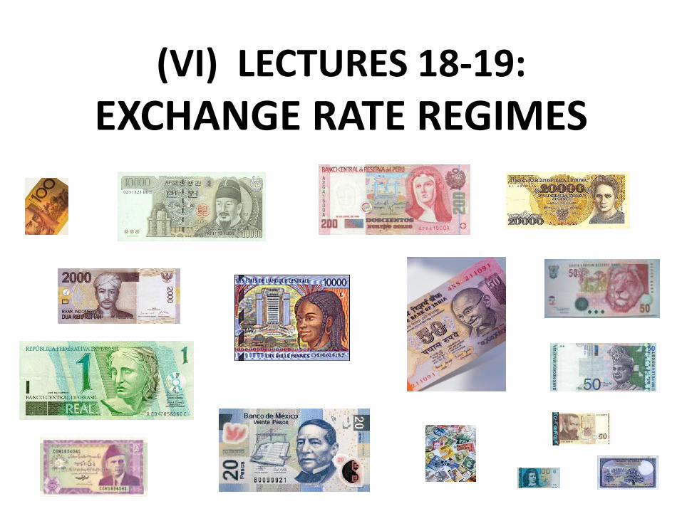
(VI) LECTURES 18-19:

EXCHANGE RATE REGIMES

Professor Jeffrey Frankel

Topics to be covered

I. Classifying countries by exchange rate regime

II. Advantages of fixed rates

III. Advantages of floating rates

IV. Which regime dominates? ● Tests

● Optimum Currency Areas

V. Additional factors for developing countries • Emigrants’ remittances

• Financial development

• Terms-of-trade shocks.

VI. Intermediate regimes & the corners hypothesis

Appendices

Continuum from flexible to rigid

FLEXIBLE CORNER

1) Free float 2) Managed float

INTERMEDIATE REGIMES

3) Target zone/band 4) Basket peg

5) Crawling peg 6) Adjustable peg

FIXED CORNER

7) Currency board 8) Dollarization

9) Monetary union

I. Classification by exchange rate regime

Trends in distribution of EM exchange rate regimes

Ghosh, Ostry & Qureshi, 2013, “Exchange Rate

Management and Crisis Susceptibility: A Reassessment,” IMF ARC , Nov..

• 1973-1985 – Many abandoned fixed exchange rates • 1986-94 – Exchange rate-based stabilization programs • 1990s -- Corners Hypothesis: countries move to either hard peg or free float • Since 2001 -- The rise of the “managed float” category.

}

Distribution of Exchange Rate Regimes in Emerging Markets, 1980-2011

(percent of total)

• Many countries that say they float, in fact intervene heavily in the foreign exchange market. [1]

• Many countries that say they fix, in fact devalue when trouble arises. [2]

• Many countries that say they target a basket of major currencies in fact fiddle with the weights. [3]

[1] “Fear of floating” -- Calvo & Reinhart (2001, 2002); Reinhart (2000).

[2] “The mirage of fixed exchange rates” -- Obstfeld & Rogoff (1995).

[3] Parameters kept secret -- Frankel, Schmukler & Servén (2000).

De jure regime de facto

One statistical approach to ascertain de facto regimes: Var (exchange rate) vs. Var (reserves).

• Calvo & Reinhart (2002) note that many countries that de jure say they float in fact have a lower Var (Δe) relative to Var (ΔRes) than many that say they fix !

• Levy-Yeyati & Sturzenegger (2005)

classify all countries based on variability of Δe vs. variability of ΔRes.

The de facto schemes do not agree.

• That de facto schemes to classify exchange rate regimes differ from the IMF’s previous de jure classification is by now well-known.

• It is less well-known that the de facto schemes also do not agree with each other !

Professor Jeffrey Frankel

Correlations Among Regime Classification Schemes

Sample: 47 countries. From Frankel, ADB, 2004. Table 3, prepared by M. Halac & S.Schmukler.

IMF GGW LY-S R-R

IMF 1.00

(100.0)

GGW 0.60 (55.1)

1.00 (100.0)

LY-S 0.28 (41.0)

0.13 (35.3)

1.00 (100.0)

R-R 0.33

(55.1) 0.34 (35.2)

0.41 (45.3)

1.00 (100.0)

(Frequency of outright coincidence, in %, given in parenthesis.)

GGW =Ghosh, Gulde & Wolf. LY-S = Levy-Yeyati & Sturzenegger. R-R = Reinhart & Rogoff

Professor Jeffrey Frankel

II. Advantages of fixed rates

1) Encourage trade <= lower exchange risk.

• True, in theory, can hedge risk. But costs of hedging:

missing markets, transactions costs, and risk premia.

• Empirical: Exchange rate volatility ↑ => trade ↓ ?

Time-series evidence showed little effect. But more in:

- Cross-section evidence,

especially small & less developed countries.

- Currency unions: Rose (2000).

The Rose finding

• Rose (2000) -- the boost to bilateral trade from currency unions is: – significant, – ≈ FTAs, & – larger (2- or 3-fold) than had been previously thought.

• Many others have advanced critiques of Rose research. – Re: sheer magnitude

• endogeneity, • small countries, • missing variables.

– Estimated magnitudes are often smaller, but the basic finding has withstood perturbations and replications remarkably well. ii/

• Some developing countries seeking regional integration talk of following Europe’s lead, though plans merit skepticism.

[ii] E.g., Rose & van Wincoop (2001); Tenreyro & Barro (2003). Survey: Baldwin (2006)

Advantages of fixed rates, cont.

2) Encourage investment <= cut currency premium out of interest rates

3) Provide nominal anchor for monetary policy • Barro-Gordon model of time-consistent inflation-fighting

• But which anchor? Exchange rate target vs. Alternatives

4) Avoid competitive depreciation (“currency wars”)

5) Avoid speculative bubbles that afflict floating.

(vs. if variability is fundamental real exchange rate risk, it will just pop up in prices instead of nominal exchange rates).

Professor Jeffrey Frankel

III. Advantages of floating rates

1. Monetary independence

2. Automatic adjustment to trade shocks

3. Retain seigniorage

4. Retain Lender of Last Resort ability

5. Avoiding crashes that hit pegged rates. (This is an advantage especially if origin of speculative attacks is multiple equilibria, not fundamentals.)

Monetary independence: Foreign interest rates have a negative impact on GDP in pegged countries; but

flexible exchange rates do insulate according to this study.

1 2 3 4

Full sample Nonpegs Pegs Full sample

Base i − 0.046 0.046 − 0.137** 0.046 0.032 0.039 0.044 0.039

Base i × Peg − 0.183**

0.055

Peg 0.014**

0.004

Constant 0.036** 0.030** 0.043** 0.030** 0.002 0.003 0.003 0.003

Observations 3831 2078 1753 3831

R2 0.001 0.001 0.009 0.005

† or other base country ** Significant at 1%. Robust standard errors clustered at country level

di Giovanni & Shambaugh (2008), JIE, "The impact of foreign interest rates on the economy: The role of the exchange rate regime."

The effects of US† interest rate i on real output growth (Sample: 1973-2002):

Professor Jeffrey Frankel

IV. Which dominate: advantages of fixing or advantages of floating?

Performance by category is inconclusive.

• To over-simplify findings of 3 studies: – Ghosh, Gulde & Wolf: hard pegs work best

– Sturzenegger & Levy-Yeyati: floats perform best

– Reinhart-Rogoff: limited flexibility is best !

• Why the different answers? – The de facto schemes do not correspond to each other.

– Conditioning factors (beyond, e.g., rich vs. poor).

Which dominate: advantages of fixing or advantages of floating?

Answer depends on circumstances, of course:

No one exchange rate regime is right for all countries or all times.

• Traditional criteria for choosing - Optimum Currency Area. Focus is on trade and stabilization of business cycle.

• 1990s criteria for choosing – Focus is on financial markets and stabilization of speculation.

Professor Jeffrey Frankel

Optimum Currency Area Theory (OCA)

Broad definition: An optimum currency area is a region that should have its own currency and own monetary policy.

This definition can be given more content:

An OCA can be defined as: a region that is neither so small & open that it would be better off pegging its currency to a neighbor, nor so large & heterogenious that it would be better off splitting into sub-regions with different currencies.

Professor Jeffrey Frankel

Optimum Currency Area criteria for giving up currency independence:

• Small size and openness

– because then advantages of fixing are large.

• Symmetry of shocks – because then giving up monetary independence is a small loss.

• Labor mobility – because then it is possible to adjust to shocks even without

ability to expand money, cut interest rates or devalue.

• Fiscal transfers in a federal system – because then consumption is cushioned in a downturn.

Professor Jeffrey Frankel

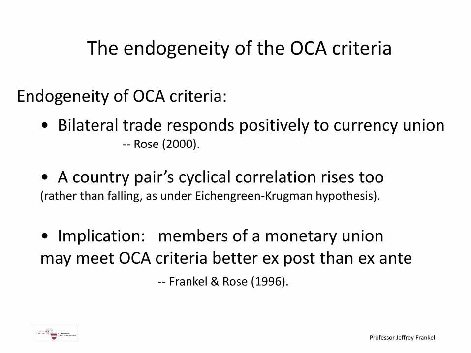
The endogeneity of the OCA criteria

Endogeneity of OCA criteria:

• Bilateral trade responds positively to currency union -- Rose (2000).

• A country pair’s cyclical correlation rises too (rather than falling, as under Eichengreen-Krugman hypothesis).

• Implication: members of a monetary union may meet OCA criteria better ex post than ex ante -- Frankel & Rose (1996).

Popularity in 1990s of institutionally-fixed corner

• currency boards (e.g., Hong Kong, 1983- ; Lithuania, 1994- ;

Argentina, 1991-2001; Bulgaria, 1997- ;

Estonia 1992-2011; Bosnia, 1998- ; …)

• dollarization

(e.g, Panama, El Salvador, Ecuador)

• monetary union

(e.g., EMU, 1999)

1990’s criteria for the firm-fix corner suiting candidates for currency boards or union (e.g. Calvo)

Regarding credibility:

Regarding other “initial conditions”: • an already-high level of private dollarization

• high pass-through to import prices

• access to an adequate level of reserves

• the rule of law.

• a desperate need to import monetary stability, due to: – history of hyperinflation,

– absence of credible public institutions,

– location in a dangerous neighborhood, or

– large exposure to nervous international investors

• a desire for close integration with a particular neighbor or trading partner

V. Three additional considerations, particularly relevant to developing countries

• (i) Emigrants’ remittances

• (ii) Level of financial development

• (iii) Supply shocks and

external terms of trade shocks

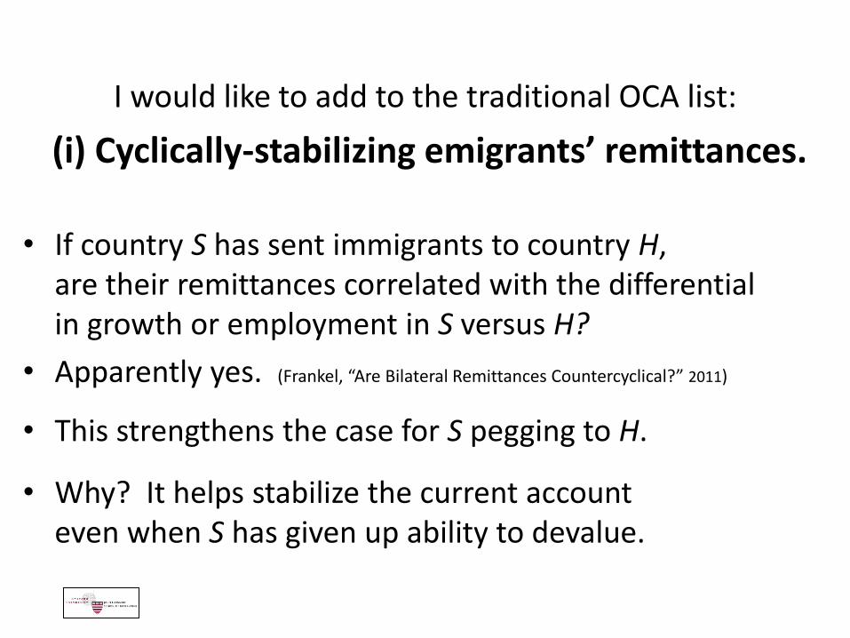
I would like to add to the traditional OCA list:

(i) Cyclically-stabilizing emigrants’ remittances.

• If country S has sent immigrants to country H, are their remittances correlated with the differential in growth or employment in S versus H?

• Apparently yes. (Frankel, “Are Bilateral Remittances Countercyclical?” 2011)

• This strengthens the case for S pegging to H.

• Why? It helps stabilize the current account even when S has given up ability to devalue.

(ii) Level of financial development

• Aghion, Bacchetta, Ranciere & Rogoff (2005)

– Fixed rates are better for countries at low levels of financial development: markets are thin.

– When financial markets develop, exchange flexibility becomes more attractive. • Estimated threshold: Private Credit/GDP > 40%.

• Husain, Mody & Rogoff (2005)

For richer & more financially developed countries, flexible rates work better

– in the sense of being more durable

– & delivering higher growth without inflation.

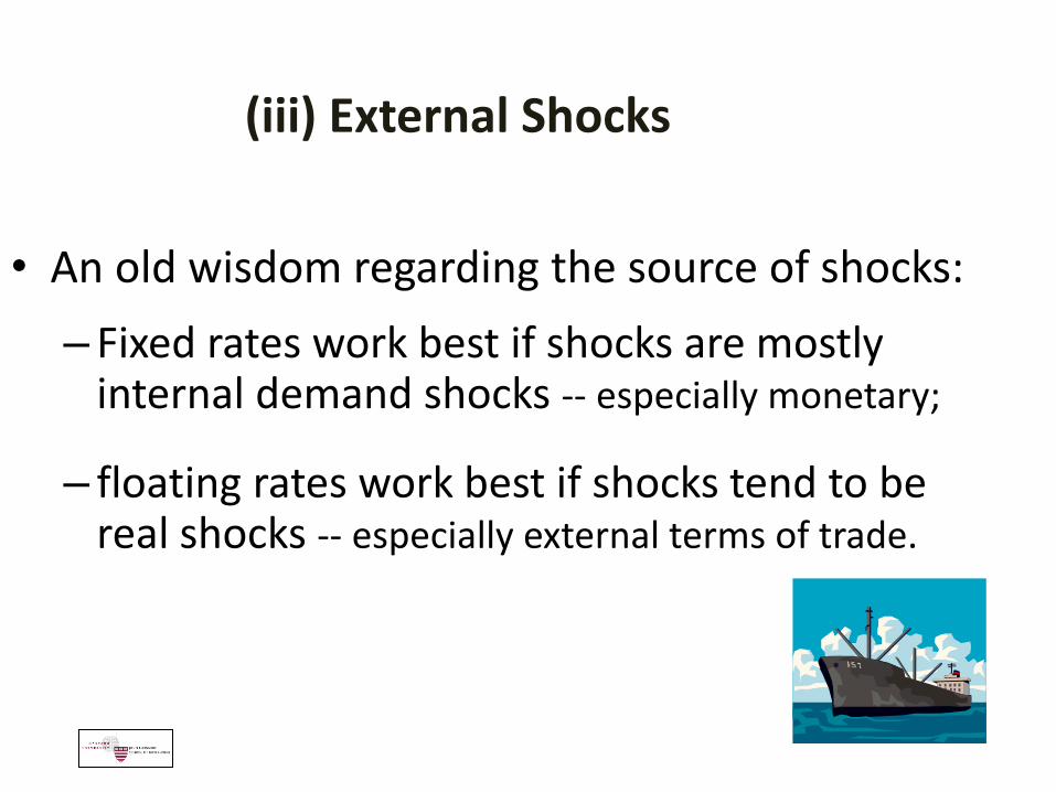
(iii) External Shocks

• An old wisdom regarding the source of shocks:

– Fixed rates work best if shocks are mostly internal demand shocks -- especially monetary;

– floating rates work best if shocks tend to be real shocks -- especially external terms of trade.

Terms-of-trade variability

• Prices of crude oil and other agricultural & mineral commodities hit record highs in 2008 & 2011.

• => Favorable terms of trade shocks for some (oil producers, such as Mideast, Africa, Latin America);

• => Unfavorable terms of trade shock for others (oil importers such as India, Korea, Turkey).

• Textbook theory says a country where trade shocks dominate should accommodate by floating.

• Confirmed empirically: – Developing countries facing terms of trade shocks do better

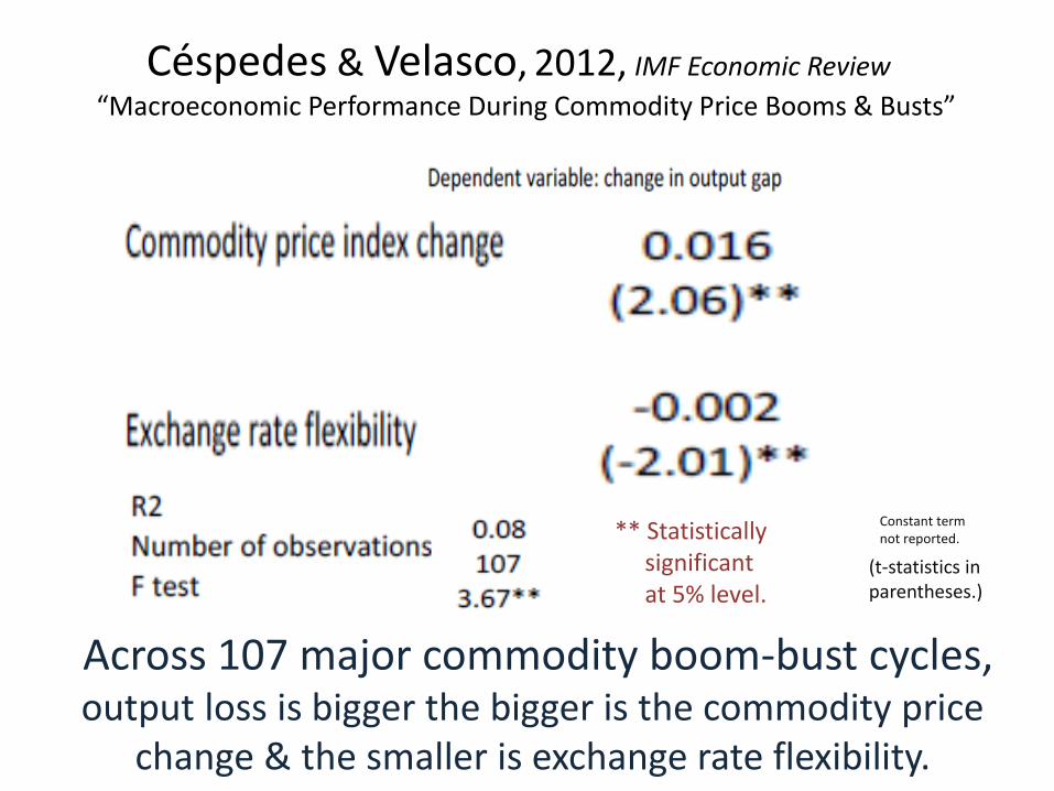
with flexible exchange rates than fixed exchange rates. – Broda (2004), Edwards & L.Yeyati (2005), Rafiq (2011),

and Céspedes & Velasco (2012)

26

Constant term not reported.

(t-statistics in parentheses.)

** Statistically significant at 5% level.

Across 107 major commodity boom-bust cycles, output loss is bigger the bigger is the commodity price

change & the smaller is exchange rate flexibility.

Céspedes & Velasco, 2012, IMF Economic Review “Macroeconomic Performance During Commodity Price Booms & Busts”

VI. Intermediate exchange rate regimes

and the corners hypothesis

Intermediate regimes

• target zone (band)

•Krugman-ERM type (with nominal anchor)

•Bergsten-Williamson type (FEER adjusted automatically)

• basket peg (weights can be either transparent or secret)

• crawling peg • pre-announced (e.g., tablita) • indexed (to fix real exchange rate)

• adjustable peg (escape clause, e.g., contingent on terms of trade or reserve loss)

• Managed float (leaning against the wind)

Origins: • 1992-93 ERM crises -- Eichengreen (1994)

• Late-90’s crises in emerging markets – Fischer (2001).

But the pendulum swung back,

• from 61% of IMF staff in 2002, to 0% in 2010. • Many developing countries follow intermediate exchange rate regimes. • The theoretical rationale for the corners hypothesis never was clear.

The Corners Hypothesis

• The hypothesis: “Countries are, or should be,

abandoning intermediate regimes like target zones

and moving to either one corner or the other: rigid peg or free float.

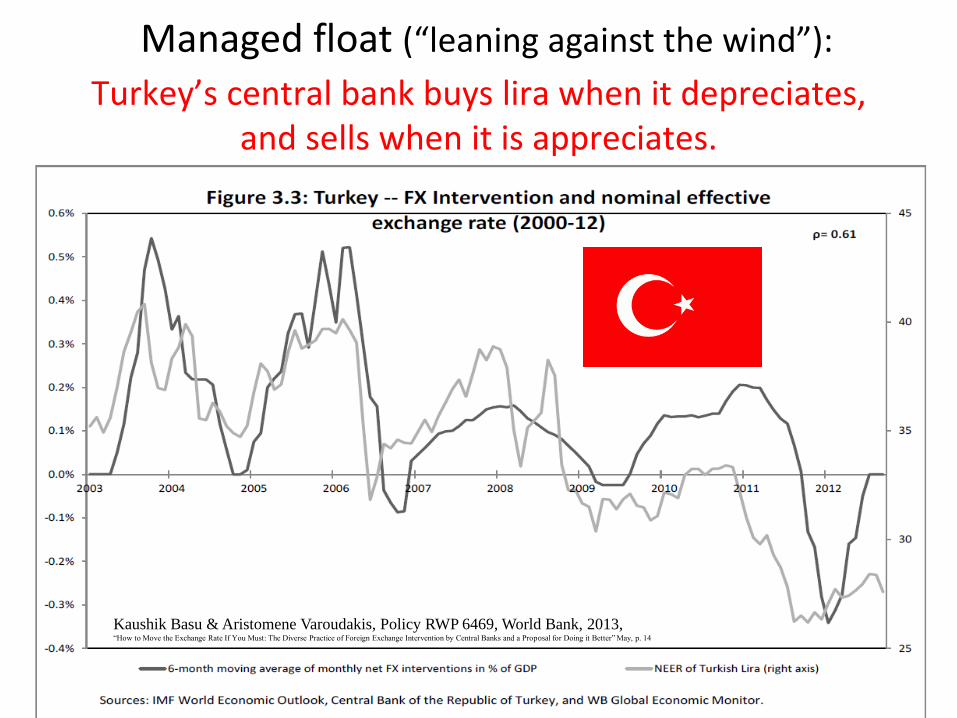
Managed float (“leaning against the wind”):

Kaushik Basu & Aristomene Varoudakis, Policy RWP 6469, World Bank, 2013, “How to Move the Exchange Rate If You Must: The Diverse Practice of Foreign Exchange Intervention by Central Banks and a Proposal for Doing it Better” May, p. 14

Turkey’s central bank buys lira when it depreciates, and sells when it is appreciates.

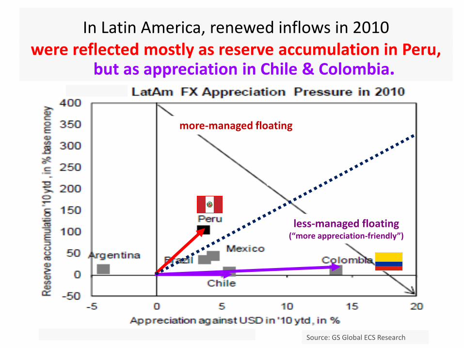
In Latin America, renewed inflows in 2010

less-managed floating (“more appreciation-friendly”)

more-managed floating

Source: GS Global ECS Research

but as appreciation in Chile & Colombia. were reflected mostly as reserve accumulation in Peru,

Korea & Singapore in 2010 took renewed inflows mostly in the form of reserves,

Goldman Sachs Global ECS Research

less-managed floating (“more appreciation-friendly”)

more-managed floating

while India & Malaysia took them mostly in the form of currency appreciation.

The flexibility parameter can be estimated in terms of Exchange Market Pressure:

– Define Δ EMP = Δ value of currency + Δ reserves/MB.

–Δ EMP represents shocks in currency demand.

– Flexibility can be estimated as the propensity of the central bank to let shocks show up in the price of the currency (floating) , vs. the quantity of the currency (fixed), or in between (intermediate exchange rate regime).

Distillation of technique to infer flexibility

• When a shock raises international demand for the currency, does it show up as an appreciation, or as a rise in reserves?

• EMP variable appears on the RHS of the equation. The % rise in the value of the currency appears on the left.

– A coefficient of 0 on EMP signifies a fixed E (no changes in the value of the currency),

– a coefficient of 1 signifies a freely floating rate (no changes in reserves) and

– a coefficient somewhere in between indicates a correspondingly flexible/stable intermediate regime.

APPENDICES ON EXCHANGE RATE REGIMES

• Appendix 1: Tables comparing economic performance of different regimes

• Appendix 2: The econometrics of estimating de facto exchange rate regimes.

•Appendix 3: IT versus alternative anchors, with volatility in commodity export prices

Appendix 1

Tables comparing economic performance of different regimes: – Ghosh, Gulde & Wolf

– Sturzenegger & Levy-Yeyati

– Reinhart & Rogoff

Which category experienced the most rapid growth?

Levy-Yeyati & Sturzenegger: floating

Reinhart & Rogoff: limited flexibility

Ghosh, Gulde & Wolf: currency boards

Levy-Yeyati & Sturzenegger (2001): floats work best.

Levy-Yeyati &

Sturzenegger (2001).

Sample: yearly

observations 1974-1999.

Effect of regime on growth rates, controlling for various determinants

Appendix 2: The econometrics of estimating de facto exchange rate regimes.

• Why do the various schemes for classifying countries by de facto exchange rate regimes give such different answers?

• Synthesis of the technique for estimating the anchor and the technique for estimating the degree of exchange rate flexibility.

Schemes for de facto classification

• have themselves been divided into two classifications, viewed as:

– “mixed de jure-de facto classifications, because the self-declared regimes are adjusted

by the devisers for anomalies.”

– Vs. “pure de facto classifications because…assignment

of regimes is based solely on statistical algorithms….”

-- Tavlas, Dellas & Stockman (2006).

Professor Jeffrey Frankel

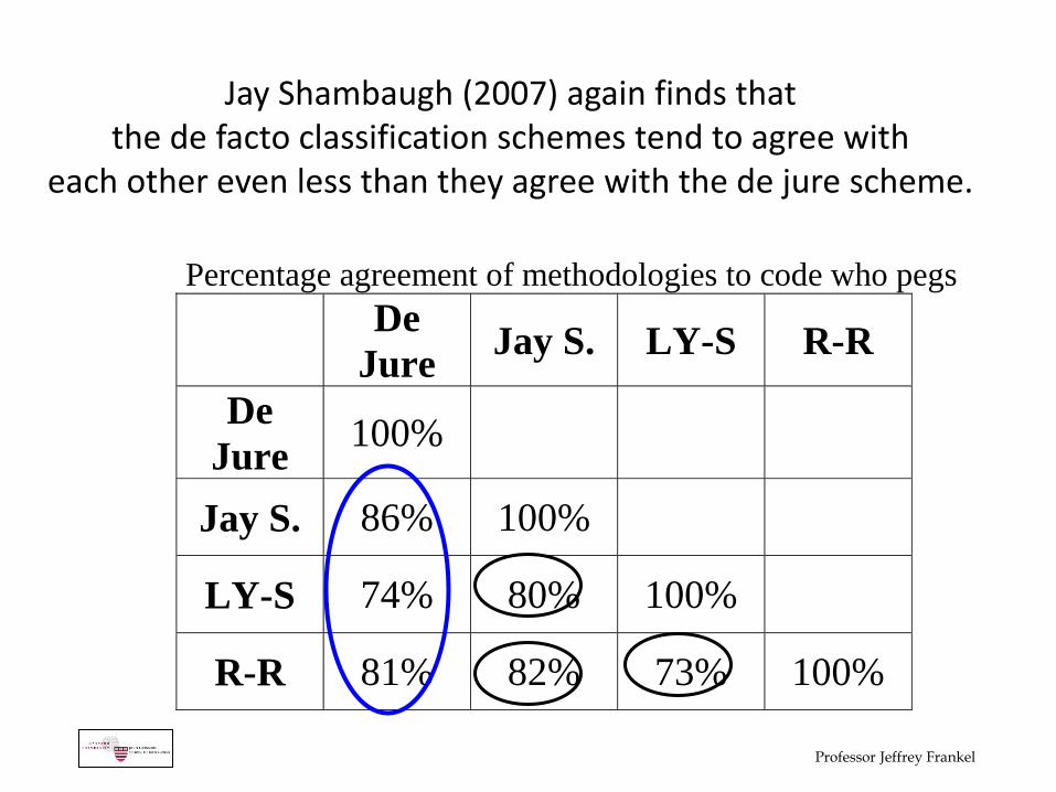
Jay Shambaugh (2007) again finds that the de facto classification schemes tend to agree with

each other even less than they agree with the de jure scheme.

Percentage agreement of methodologies to code who pegs

De

Jure Jay S. LY-S R-R

De

Jure 100%

Jay S.

86% 100%

LY-S

74% 80% 100%

R-R

81% 82% 73% 100%

-- but still close to official IMF one: correlation (BOR, IMF) = .76

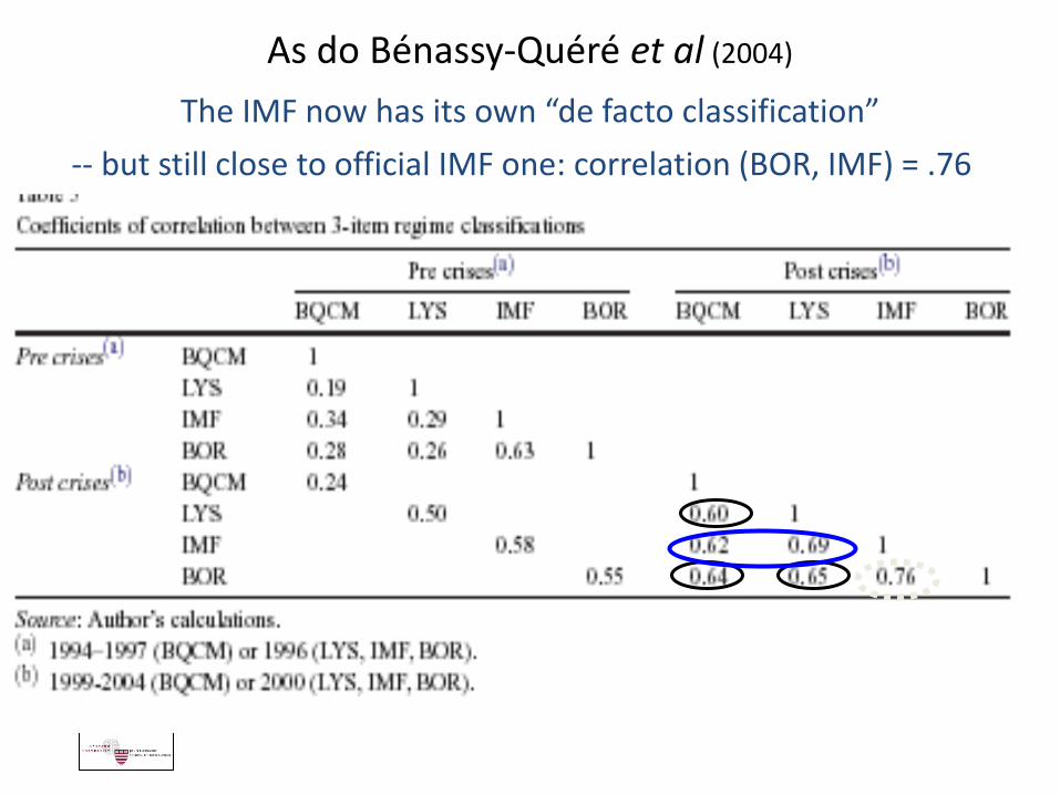
The IMF now has its own “de facto classification”

As do Bénassy-Quéré et al (2004)

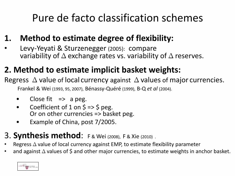
Pure de facto classification schemes

1. Method to estimate degree of flexibility: • Levy-Yeyati & Sturzenegger (2005): compare

variability of Δ exchange rates vs. variability of Δ reserves.

2. Method to estimate implicit basket weights: Regress Δ value of local currency against Δ values of major currencies. Frankel & Wei (1993, 95, 2007), Bénassy-Quéré (1999), B-Q et al (2004).

• Close fit => a peg. • Coefficient of 1 on $ => $ peg.

Or on other currencies => basket peg. • Example of China, post 7/2005.

3. Synthesis method: F & Wei (2008), F & Xie (2010) .

• Regress Δ value of local currency against EMP, to estimate flexibility parameter • and against Δ values of $ and other major currencies, to estimate weights in anchor basket.

Appendix 3

IT versus alternative anchor (PEP) to take into account

commodity export prices

Professor Jeffrey Frankel

Fashions in international currency policy

• 1980-82: Monetarism (target the money supply)

• 1984-1997: Fixed exchange rates (incl. currency boards)

• 1993-2001: The corners hypothesis

• 1998-2008: Inflation targeting (+ currency float)

became the new conventional wisdom • Among academic economists

• among central bankers

• and at the IMF

Professor Jeffrey Frankel

6 proposed nominal targets and the Achilles heel of each:

Targeted

variable Vulnerability Example

Monetarist rule

M1 Velocity shocks US 1982

Inflation targeting CPI

Import price

shocks Oil shocks of

1973-80, 2000-08

Nominal income

targeting

Nominal

GDP

Measurement

problems

Less developed

countries

Gold standard Price

of gold

Vagaries of world

gold market

1849 boom;

1873-96 bust

Commodity

standard

Price of agric.

& mineral

basket

Shocks in

imported

commodity

Oil shocks of

1973-80, 2000-08

Fixed

exchange rate $

(or €)

Appreciation of $ (or € )

1995-2001

Professor Jeffrey Frankel

Inflation Targeting has been the reigning orthodoxy.

• Flexible inflation targeting ≡ “Have a LR target for inflation, and be transparent.” Who could disagree?

• But define IT as setting yearly CPI targets, to the exclusion of

• asset prices

• exchange rates

• export commodity prices.

• Some reexamination is warranted, in light of 2008-2011.

Professor Jeffrey Frankel

• The shocks of 2008-2015 showed disadvantages to Inflation Targeting, – analogously to how the EM crises of the 1994-2001

showed disadvantages of exchange rate targeting.

• It gives the wrong answer in case of trade shocks:

• E.g., it says to tighten money & appreciate in response to a rise in oil import prices;

• It does not allow monetary tightening & appreciation in response to a rise in world prices of export commodities.

• That is backwards.

Proposal to Peg the Export Price

Intended for countries with volatile terms of trade, e.g., those specialized in commodities.

The authorities stabilize the currency in terms of a basket of currencies plus the price of the export commodity rather than to the CPI (which gives weight to imports)

and rather than a simple fixed exchange rate.

The regime combines the best of both worlds:

(i) The advantage of automatic accommodation to terms of trade shocks, together with

(ii) the advantages of a nominal anchor.

PEP

Professor Jeffrey Frankel

Why is PEP better than targeting the exchange rate or CPI

for countries with volatile terms of trade?

Better response to adverse terms of trade shocks:

• If the $ price of the export commodity goes up, PEP says to tighten monetary policy enough to appreciate currency. – Right response. (E.g., Gulf currencies in 2007-08.)

• If the $ price of imported commodity goes up, CPI target says to tighten monetary policy enough to appreciate currency. – Wrong response. (E.g., ECB or other oil-importers in 2007-08.)

– => CPI targeting gets it backwards.

PEP

Professor Jeffrey Frankel

Does floating give the same answer as PEP?

• True, commodity currencies tend to appreciate when commodity markets are strong, & vice versa

– Australian, Canadian & NZ $ (e.g., Chen & Rogoff, 2003)

– South African rand (e.g., Frankel, 2007)

– Chilean peso and others

• But

– Some volatility under floating appears gratuitous.

– Floaters still need a nominal anchor.

Professor Jeffrey Frankel

The Rand, 1984-2006: Fundamentals (real commodity prices,

real interest differential, country risk premium, & l.e.v.) can explain the real appreciation of 2003-06 – Frankel (SAJE, 2007).

0.000

20.000

40.000

60.000

80.000

100.000

120.000

140.000

160.000

180.000

200.000

Q2 1984

Q1 1985

Q4 1985

Q3 1986

Q2 1987

Q1 1988

Q4 1988

Q3 1989

Q2 1990

Q1 1991

Q4 1991

Q3 1992

Q2 1993

Q1 1994

Q4 1994

Q3 1995

Q2 1996

Q1 1997

Q4 1997

Q3 1998

Q2 1999

Q1 2000

Q4 2000

Q3 2001

Q2 2002

Q1 2003

Q4 2003

Q3 2004

Q2 2005

Q1 2006

RERICPIactual RERICPIFitted RERICPIProjected

Actual vs Fitted vs. Fundamentals- Projected Values

In practice, most IT proponents agree central banks should not tighten to offset oil price shocks

• They want focus on core CPI, excluding food & energy.

• But

– food & energy ≠ all supply shocks.

– Use of core CPI sacrifices some credibility: • If core CPI is the explicit goal ex ante, the public feels confused.

• If it is an excuse for missing targets ex post, the public feels tricked.

– The threat to credibility is especially strong where there are historical grounds for believing that government officials fiddle with the CPI for political purposes.

– Perhaps for that reason, IT central banks apparently do respond to oil shocks by tightening/appreciating….