Embed Size (px)
Citation preview
______________________________________________________________________________
VIBRATION ANALYSIS AND INTELLIGENT
CONTROL OF FLEXIBLE ROTOR SYSTEMS USING
SMART MATERIALS
by
Lawrence Atepor
THESIS SUBMITED IN FULFILLMENT OF THE REQUIREMENTS
FOR THE DEGREE OF DOCTOR IN PHILOSOPHY
TO THE FACULTY OF ENGINEERING
DEPARTMENT OF MECHANICAL ENGINEERING
UNIVERSITY OF GLASGOW
© L. Atepor
October 2008
All Rights Reserved
This work may not be reproduced in whole or in part, by photocopy or other
means without permission of the author.
This thesis is produced under the accordance of British standards BS 4821: 1990

i
To my Family

ii
COPYRIGHT
Attention is drawn to the fact that copyright of this thesis rests with its author.
This copy of the thesis has been supplied on the condition that anyone who
consults it is understood to recognise that its copyright rests with the author and
that no quotation from the thesis and no information derived from it may be
published, without prior written consent of the author.
This thesis may not be consulted, photocopied or lent by any library without the
permission of the author for a period of two years from the date of acceptance
of the thesis.
Abstract
_____________________________________________________________________________iii
ABSTRACT
Flexible rotor-bearing system stability is a very important subject impacting the
design, control, maintenance and operating safety. As the rotor bearing-system
dynamic nonlinearities are significantly more prominent at higher rotating
speeds, the demand for better performance through higher speeds has rendered
the use of linear approaches for analysis both inadequate and ineffective. To
address this need, it becomes important that nonlinear rotor-dynamic responses
indicative of the causes of nonlinearity, along with the bifurcated dynamic
states of instabilities, be fully studied. The objectives of this research are to
study rotor-dynamic instabilities induced by mass unbalance and to use smart
materials to stabilise the performance of the flexible rotor-system. A
comprehensive mathematical model incorporating translational and rotational
inertia, bending stiffness and gyroscopic moment is developed. The dynamic end
conditions of the rotor comprising of the active bearing-induced axial force is
modelled, the equations of motion are derived using Lagrange equations and the
Rayleigh-Ritz method is used to study the basic phenomena on simple systems. In
this thesis the axial force terms included in the equations of motion provide a
means for axially directed harmonic force to be introduced into the system. The
Method of Multiple Scales is applied to study the nonlinear equations obtained
and their stabilities. The Dynamics 2 software is used to numerically explore the
inception and progression of bifurcations suggestive of the changing rotor-
dynamic state and impending instability.
In the context of active control of flexible rotors, smart materials particularly
SMAs and piezoelectric stack actuators are introduced. The application of shape
memory alloy (SMA) elements integrated within glass epoxy composite plates and
shells has resulted in the design of a novel smart bearing based on the principle
of antagonistic action in this thesis. Previous work has shown that a single
SMA/composite active bearing can be very effective in both altering the natural
frequency of the fundamental whirl mode as well as the modal amplitude. The
drawback with that design has been the disparity in the time constant between
the relatively fast heating phase and the much slower cooling phase which is
reliant on forced air, or some other form of cooling. This thesis presents a
modified design which removes the aforementioned existing shortcomings. This
form of design means that the cooling phase of one half, still using forced air, is
Abstract
iv
significantly assisted by switching the other half into its heating phase, and vice
versa, thereby equalising the time constants, and giving a faster push-pull load
on the centrally located bearing; a loading which is termed ‘antagonistic’ in this
present dissertation. The piezoelectric stack actuator provides an account of an
investigation into possible dynamic interactions between two nonlinear systems,
each possessing nonlinear characteristics in the frequency domain. Parametric
excitations are deliberately introduced into a second flexible rotor system by
means of a piezoelectric exciter to moderate the response of the pre-existing
mass-unbalance vibration inherent to the rotor. The intended application area
for this SMA/composite and piezoelectric technologies are in industrial rotor
systems, in particular very high-speed plant, such as small light pumps, motor
generators, and engines for aerospace and automotive application.

Acknowledgements
_____________________________________________________________________________v
ACKNOWLENDGEMENTS
I am so grateful to God who has made this research possible and to those who
have made my experience in the University of Glasgow one that I will always
remember fondly.
Firstly, I would like to express my sincere gratitude to my supervisor, Professor
Matthew Philip Cartmell, who has been like a father and a mentor to me. His
advice and guidance throughout the course or my postgraduate studies were
invaluable, as was his patience and politeness that never failed during his
supervision. I have learnt a lot of positive things from him. Thank you for being
an advisor, a mentor and a good friend.
Thanks also extend out to Mr. Brian Robb and Mr. Bernie Hoey who have been of
great help to me in the fixing of my experimental rigs, and to Dr. Asif Israr, my
office mate for three years, for his encouragement and for being a good office
mate.
Also to the Ghana Education Trust Fund (GetFund) and the Ghana Scholarship
Secretariat who provided me with the scholarships for this course of study, and
the Dynamics Group of the Mechanical Engineering Department, University of
Glasgow for their support and for the provision of the necessary facilities and
equipment; these are greatly appreciated.
Lastly to my friends, the Tuwor family in Glasgow, and to my family for their
never ending support, sacrifices, understanding and encouragement throughout
my course of studying at the University of Glasgow. Without them, I would not
have been able to achieve what I have today.
“Thank you so very much and may God bless you richly”
List of Figures
_____________________________________________________________________________vi
LIST OF FIGURES
Figure 2-1: Typical temperature-transformation curves of a NiTi alloy (Marc van
der Wijst 1998). ........................................................................... 30
Figure 2-2: Schematic cross-section of piezoelectric stack actuator .............. 32
Figure 3-1: Reference frames for a disk on a rotating flexible shaft. ............. 37
Figure 3-2: Coordinates of the geometric centre c and an arbitrary point B on
the shaft (Lalanne & Ferraris, 1990) ................................................... 40
Figure 3- 3: Mass Unbalance ............................................................. 44
Figure 3- 4: Coordinates.................................................................. 46
Figure 3- 5: Bearing stiffness and damping............................................ 50
Figure 4-1: Amplitudes of the response as functions of the frequency at mass
unbalance mu=0.004kg and damping coefficient of 13.6 Ns/m. .................... 81
Figure 4- 2: Amplitudes of the response as functions of the frequency at mass
unbalance 3mu and damping coefficient of 13.6 Ns/m. ............................. 82
Figure 4- 3: Amplitudes of the response as functions of the frequency at mass
unbalance mu and damping coefficient of 15 Ns/m. ................................. 82
Figure 4- 4: Amplitudes of the response as functions of the frequency at mass
unbalance mu and damping coefficient of 13.6 Ns/m with parametric force term.
............................................................................................... 82
Figure 4- 5: Amplitudes of the response as functions of the frequency........... 85
Figure 4- 6: Amplitudes of the response as functions of the frequency at the
inclusion of parametric force term. .................................................... 85
Figure 4- 7: Plots of response for MMS and Numerical Integration together-
without parametric force terms......................................................... 86
Figure 4- 8: Plots of response for MMS and Numerical Integration together- with
parametric force terms................................................................... 86
Figure 5- 1: Stability plots for k values................................................100
Figure 5- 2: Stability plots for λ values ...............................................101
Figure 6- 1: Sketch of the change in distance between two nearby orbits used to
define Lyapunov exponent ..............................................................110
Figure 6- 2: Bifurcation diagrams showing amplitude as a function of Ω (X-
axis:Ω ,Y-axis: 1x , 2x ), where 1 2x x x= = ..............................................113
List of Figures
vii
Figure 6- 3: Lyapunov exponent and Bifurcation diagrams of amplitude as a
function of the normalised excitation acceleration in the horizontal direction.
..............................................................................................114
Figure 6- 4: Lyapunov exponent and Bifurcation diagrams of amplitude as a
function of the normalised excitation acceleration for the Model with Parametric
force term in the horizontal direction. ...............................................115
Figure 6- 5: Dynamical analysis of response to normalised excitation acceleration
at 250 in the horizontal direction......................................................121
Figure 6- 6: Dynamical analysis of response to normalised excitation acceleration
at 400 in the horizontal direction......................................................122
Figure 6- 7: Dynamical analysis of response to normalised excitation acceleration
at 460 in the horizontal direction......................................................123
Figure 6- 8: Dynamical analysis of response to normalised excitation acceleration
at 505 in the horizontal direction......................................................124
Figure 6- 9: Dynamical analysis of response to normalised excitation acceleration
at 618 in the horizontal direction......................................................125
Figure 6- 10: Dynamical analysis of response to normalised excitation
acceleration at 840 in the horizontal direction......................................125
Figure 6- 11: Dynamical analysis of response to normalised excitation
acceleration of models with the parametric force term in the horizontal
direction ...................................................................................126
Figure 6- 12: Poincaré maps for the Models from solutions obtained from bespoke
integration code in MathematicaTM. ...................................................128
Figure 6- 13: Phase planes and Time plots for mu from solutions obtained from
bespoke integration code in MathematicaTM. ........................................129
Figure 6- 14: Phase planes and Time plots for 3mu from solutions obtained from
bespoke integration code in MathematicaTM. ........................................130
Figure 6- 15: Phase planes and Time plots for 4mu from solutions obtained from
bespoke integration code in MathematicaTM. ........................................131
Figure 6- 16: Phase planes and Time plots for 5mu from solutions obtained from
bespoke integration code in MathematicaTM. ........................................132
Figure 6- 17: Dynamical analysis of response to normalised excitation
acceleration at the various discrete points from solutions obtained from
integration code in MathematicaTM ....................................................133
List of Figures
viii
Figure 7- 1: SMA Experimental set-up for response measurements...............137
Figure 7- 2: Schematic view of Instruments used for the Antagonistic
SMA/Composite Smart Bearing experiment...........................................138
Figure 7- 3: The Antagonistic SMA/Composite Smart Bearing Test Rig ...........138
Figure 7- 4: Schematic of the antagonistic SMA/Composite bearing housing....140
Figure 7- 5: The amplitudes of disc vibration versus excitation frequency for the
right hand side of the Antagonistic Bearing. .........................................143
Figure 7- 6: The amplitudes of disc vibration versus excitation frequency for the
left hand side of the Antagonistic Bearing............................................143
Figure 7- 7 : Close-up of the Piezoelectric Exciter ..................................147
Figure 7- 8: Assembly of the Piezoexciter Test Rig..................................147
Figure 7- 9: (a) Shaft-end assembly when rotor is not whirling, (b) Shaft-end
assembly when rotor is whirling at maximum amplitude and (c) Free length of
spring.......................................................................................150
Figure 7- 10: Schematic of the piezoelectric exciter. ..............................151
Figure 7- 11: The amplitudes of disc vibration versus frequency with a spring
compression length of 20.2mm.........................................................155
Figure 7- 12: The amplitudes of disc vibration versus frequency with a spring
compression length of 25.2mm.........................................................156
Figure A.1- 1: Model of the rotor ......................................................A-2
Figure A.1- 2: Schematic of the shafts movements. ................................A-5
Figure C- 1: Dynamics 2 Program Code for coupled Duffing equations ...........C-1

List of Tables
_____________________________________________________________________________ix
LIST OF TABLES
Table 4- 1: Data of graphs plotted...................................................... 81
Table 5- 1: Summary of conditions for stability according to Routh’s criterion . 96
Table 5- 2: Discrete mass unbalance values with their stability indicators....... 99
Table 6- 1: Data used for numerical simulations ....................................107
Table 6- 2: Program command values for Dynamic 2 Plotting .....................109
Table 7- 1: Material properties of a typical SMA material (Ni-Ti alloy),
(http:www.sma-inc.com)................................................................142

Table of Contents
_____________________________________________________________________________x
TABLE OF CONTENTS
COPYRIGHT........................................................................................................... ii
ABSTRACT ........................................... ................................................................ iii
ACKNOWLENDGEMENTS.................................. ..................................................v
LIST OF FIGURES ................................................................................................ vi
LIST OF TABLES..................................... ............................................................. ix
TABLE OF CONTENTS .................................. .......................................................x
NOMENCLATURE ....................................... ........................................................ xv
CHAPTER 1............................................................................................................1
INTRODUCTION ....................................................................................................1
1.1 Background......................................... .......................................................... 1
1.2 Objectives ......................................... ............................................................ 3
1.3 Outline and Methodology............................ ................................................. 5
CHAPTER 2............................................................................................................7
LITERATURE REVIEW .................................. ........................................................7
2.1 Historical Perspective ............................. ..................................................... 7
2.1.1 Jeffcott’s Rotor ...............................................................................................7
2.1.2 Origins of Vibration Theory.............................................................................8
2.1.3 Gyroscopic Effects .........................................................................................8
2.1.4 Shape Memory Alloys ....................................................................................9
2.1.5 Piezoelectric Materials ...................................................................................9
2.2 Vibration Control of Rotor Systems................. ......................................... 10
2.3 Nonlinearities in Structures....................... ................................................ 14
2.3.1 Types of Nonlinearity....................................................................................15
2.3.2 Nonlinearities of Beams/ Shafts ...................................................................17
2.3.3 Nonlinearities in Bearings.............................................................................18
2.4 Nonlinear Control .................................. ..................................................... 20
Table of Contents
xi
2.5 Perturbation Methods............................... .................................................. 22
2.6 Method of Multiple Scales (MMS) .................... .......................................... 23
2.7 Smart Materials.................................... ....................................................... 26
2.8 Shape Memory Alloy (SMA) ........................... ............................................ 28
2.9 Piezoelectric Materials ............................ ................................................... 31
CHAPTER 3..........................................................................................................34
ANALYTICAL MODELLING OF FLEXIBLE ROTOR SYSTEMS ..... ...................34
3.1 Introduction....................................... .......................................................... 34
3.2 Derivation of the Equations of Motion .............. ........................................ 35
3.2.1 Rotor Model .................................................................................................36
3.2.2 Kinetic Energy of the Rotating Disk ..............................................................38
3.2.3 Kinetic Energy of the Shaft...........................................................................39
3.2.4 Strain Energy of the Shaft ............................................................................40
3.2.5 Kinetic Energy of the Mass Unbalance.........................................................43
3.2.6 Simplified Model...........................................................................................45
3.2.7 Nonlinear Bearing ........................................................................................48
3.2.8 Equations of Motion .....................................................................................52
3.2.8.1 Alternative Analytical Model A .............................................................................53
3.2.8.2 Alternative Analytical Model B .............................................................................53
3.2.8.3 Alternative Analytical Model C.............................................................................54
3.2.9 Linear Viscous Damping ..............................................................................54
3.2.9.1 Model A................................................................................................................54
3.2.9.2 Model B................................................................................................................55
3.2.9.3 Model C ...............................................................................................................55
3.2.10 Parameter Estimation Procedure .................................................................55
3.2.10.1 Nonlinearity Estimation ........................................................................................56
3.2.11 Discussions..................................................................................................57
CHAPTER 4..........................................................................................................58
APPROXIMATE ANALYTICAL AND NUMERICAL SOLUTIONS TO T HE
EQUATIONS OF MOTION ...................................................................................58
4.1 Introduction....................................... .......................................................... 58
Table of Contents
xii
4.2 Ordering of Terms .................................. .................................................... 59
4.3 The Method of Multiple Scales ...................... ............................................ 62
4.3.1 Introducing the Time Scales .........................................................................62
4.3.2 Treatment of Coefficients to like Orders of ε ..............................................63
4.3.3 Secular Terms to First Order Perturbation....................................................65
4.3.4 Modulation of First Order Perturbation Equations.........................................68
4.3.5 Second Order Perturbation Equations..........................................................70
4.3.6 Secular Terms from the Second Order Perturbation Equations ....................71
4.3.7 Analysis of the Second Order Solvability Equations .....................................72
4.3.8 General Solutions of the Equations of Motion (4.2-1) and (4.2-2) .................77
4.3.9 Multiple Scales Results ................................................................................80
4.3.9.1 Amplitude Response Plot – without Parametric Force Term...............................81
4.3.9.2 Amplitude Response Plot – with Parametric Force Term....................................82
4.4 Direct Numerical Integration....................... ............................................... 83
4.4.1 Results from MathematicaTM ........................................................................85
4.4.1.1 Numerical Integration Plot- without Parametric Force Term ...............................85
4.4.1.2 Numerical Integration Plot- with Parametric Force Term ....................................85
4.5 Discussion of Results .............................. .................................................. 87
CHAPTER 5..........................................................................................................88
STABILITY OF STEADY-STATE SOLUTIONS ................ ...................................88
5.1 Introduction....................................... .......................................................... 88
5.2 Stability Matrix ................................... ......................................................... 88
5.3 The Routh-Hurwitz Stability Criterion .............. ......................................... 93
5.3.1 Stability Results............................................................................................97
CHAPTER 6........................................................................................................102
INVESTIGATION OF SYSTEMS DYNAMICS.................. ..................................102
6.1 Introduction....................................... ........................................................ 102
6.2 Program Code....................................... .................................................... 103
6.2.1 Dynamics 2 Code.......................................................................................103
6.2.1.1 Nondimensionalisation ......................................................................................104
Table of Contents
xiii
6.2.2 Mathematica TM Code.................................................................................106
6.2.3 Definition of Parameters.............................................................................106
6.3 Bifurcation Analysis ............................... .................................................. 107
6.4 Lyapunov Exponents ................................. .............................................. 109
6.5 Bifurcations as Functions of Excitation Acceleratio n ........................... 110
6.6 Phase Planes, Poincaré Maps and Time Plots ......... .............................. 116
6.6.1 Analysis of Phase Planes, Poincaré Maps and Time Plots.........................117
6.6.1.1 At Normalised Excitation Acceleration of 250 (Figure 6-5): ..............................117
6.6.1.2 At Normalised Excitation Acceleration of 400 (Figure 6-6): ..............................118
6.6.1.3 At Normalised Excitation Acceleration of 460 (Figure 6-7): ..............................118
6.6.1.4 At Normalised Excitation Acceleration of 505 (Figure 6-8): ..............................119
6.6.1.5 At Normalised Excitation Acceleration of 618 (Figure 6-9) and 840 (Figure 6-10):...........................................................................................................................120
6.6.1.6 Including Parametric Force Term (Figure 6-11): ...............................................120
6.7 Numerical investigations in MathematicaTM code .................................. 126
CHAPTER 7........................................................................................................134
EXPERIMENTAL INVESTIGATIONS........................ .........................................134
7.1 Controlling Flexible Rotor Vibration by means of an
Antagonistic SMA/Composite Smart Bearing. .......... ............................. 134
7.1.1 Introduction ................................................................................................134
7.1.2 Overview of the Experimental Rig ..............................................................136
7.1.3 Active Bearing Concept..............................................................................139
7.1.4 Active Bearing Experiment .........................................................................140
7.1.5 Experimental Results .................................................................................141
7.2 Controlling Flexible Rotor Vibration by means of a Piezoelectric Stack
Exciter. ...................................................................................................... 144
7.2.1 Introduction ................................................................................................144
7.2.2 Instrumentation ..........................................................................................146
7.2.3 Design and Selection of Piezoexciter Component ......................................147
7.2.4 Test Setup..................................................................................................149
7.2.5 Experimental Results .................................................................................151
7.2.6 Piezoelectric Exciter Applications...............................................................153
Table of Contents
xiv
CHAPTER 8........................................................................................................157
DISCUSSIONS OF RESULTS............................................................................157
8.1 Introduction....................................... ........................................................ 157
8.2 Analytical Results................................. .................................................... 157
8.3 Stability Analysis Results ......................... ............................................... 159
8.4 Numerical Results .................................. .................................................. 159
8.5 Experimental Results ............................... ................................................ 162
8.6 Conclusions........................................ ...................................................... 162
CHAPTER 9........................................................................................................164
CONCLUSIONS AND RECOMMENDATIONS FOR FURTHER WORK ... ........164
9.1 Summary ............................................ ....................................................... 164
9.2 Recommendations for Further Work ................... ................................... 167
REFERENCES ...................................................................................................169
PUBLICATIONS ....................................... ..........................................................202
___________________________________________ ......................................202
CONTENTS OF APPENDICES.......................................................................... A-1
___________________________________________ ...................................... A-1
............................................................................................................................ C-1

Nomenclature
_____________________________________________________________________________xv
NOMENCLATURE
Symbols Description
1q , 2q Displacement
c , 1C Damping coefficients
ω Natural frequency
k , 3C Linear stiffness coefficient
b , 4C Nonlinear cubic stiffness coefficient
m Modal mass
θ ,φ ,ψ Angles of rotation
xω , yω , zω Angular velocities
T Kinetic energy
U Strain energy
dT Kinetic energy of disk
ST Kinetic energy of shaft
uT Kinetic energy of mass unbalance
dM Mass of disk
um Mass unbalance
Nomenclature
xvi
d Distance of mass unbalance from
geometric centre of shaft
iqF Generalised forces
iqWδ Virtual work associated with a
generalised force
E Modulus of elasticity
I Area moment of inertia
dxI , dzI , dyI Diametral moment of inertia
S Cross-sectional area of shaft
u , v , w Displacement in the x , y , z directions
*u , *w Displacement of the geometric centre
with respect to the x and z directions
xF , zF Bearing forces in the x and z directions
ijk Linear spring coefficients; , ,i j x z=
ijk Nonlinear spring coefficients; , ,i j x z=
ijc Linear damping coefficients; , ,i j x z=
nlω Nonlinear frequency
bk Bearing stiffness coefficient
bc Bearing damping coefficient
sc Damping coefficient of shaft
Nomenclature
xvii
a, b Amplitude response
τ Nondimensionalised time
T Time
nT 0n = :Fast time scales; 1,2n = :Slow time
scales i.e, 0T t= ; 1T tε= ; 22T tε=
ε Ordering parameter for method of
multiple scales
A , C Complex amplitudes
Γ , ρ Excitation amplitude
Ω Excitation frequency
ωΩ
Nondimensionalised excitation
frequency
1α , 2α Phase angles
σ Detuning parameter
2Ω Parametric excitation frequency;
2 2Ω = Ω for the case of exact principal
parametric resonance
ia Characteristic equation coefficients;
i ia k= ; 1i = to n
iλ Eigenvalues
λ Lyapunov exponent
maxSF Maximum spring force

Nomenclature
xviii
minSF Minimum spring force
SSk Spring constant
(max)actF Maximum actuator force;
(max) 0act act vF F F= =
1δ Spring ‘preload’ pre-compression
2δ Maximum spring compression
∆ Maximum shaft end displacement
BIFD No. of iterates (dots plotted) for each
bifurcation parameter
BIFPI Pre-iterates for each bifurcation
parameter
BIFV No. of parameter values in bifurcation
diagram
CON Connect consecutive dots of
trajectories
I-H-B Incremental harmonic balance
IPP No. of iterates per plot
K-B Krylov-Bogolioubov Method
K-B-M Krylov-Bogolioubov-Mitropolski Method
L-P Lindstedt-Poincaré Method
MMS Method of multiple scales
NI Direct numerical integration
Nomenclature
xix
ODE Ordinary differential equation
PI No. of pre-iterates before plotting
SMA Shape memory alloy
SPC Steps per cycle
Chapter 1: Introduction
1
CHAPTER 1
INTRODUCTION
________________________________________________________
1.1 Background
Rotating machinery play an important role in many different industries in our
society. Some examples are in electrical power production, gas-turbines, aircraft
engines, process machines in heavy industry, fans, pumps and ship engines,
which are only a few of the applications in which rotating machinery has a
central role. The designs of many rotating machines are now fifty to a hundred
years old; however, the demands of these units are continuously changing.
Hence, it becomes important to work on product development and research in
the area of rotating machinery. The behaviour of these rotor-dynamic
components can influence the performance of the whole system. Namely, for
certain ranges of rotational speed, such systems can exhibit various types of
vibration which can be so violent that it can cause significant damage.
Consequently, the understanding of the dynamic behaviour of these systems is
very important.
Vibration in dynamical systems can be caused by nonlinearities which induce
forces locally in the system under consideration. However, their presence in
general has important consequences for the overall dynamic behaviour. Some
examples of nonlinearities in mechanical systems are friction forces, mass
unbalance, and nonlinear spring and damper supports. Therefore, in order to
gain understanding and to predict different types of vibration it is important to
understand the causes of such vibrations, and also to understand the interactions
between them where there exists more than one type of vibration. Lateral
vibrations in rotor systems have been analysed extensively by Tondl, 1965; Fritz,
1970 (a, b) and Lee, 1993. They considered different types of rotor systems, and
in all those systems, lateral vibrations are induced by the mass unbalance in a
rotor. In all the systems considered it is noticed that increase of mass unbalance
can have destabilising effects. For example, Tondl, 1965 and Lee, 1993
Chapter 1: Introduction
2
considered a simple disk with a mass unbalance connected to a shaft which is
elastic in the lateral direction and found out that in such systems, under certain
conditions, instabilities can appear if the mass unbalance increases. Since the
rotating parts of these machines are mostly the main sources of vibration,
adequate understanding and knowledge of the vibration phenomena of rotor-
dynamics are necessary for finding ways to reduce or eliminate when possible
vibrations. It has been observed that when the running speed exceeds certain
critical speeds, various kinds of undesirable problems of rotor-dynamic
instability would occur. Therefore, studying the static and dynamic response,
both theoretically and experimentally, of the flexible rotor system under various
loading conditions would help in understanding and explaining the behaviour of
more complex, real structures under similar conditions.
The analysis of the nonlinear effects in rotor-bearing systems is extremely
difficult and there are a few analytical procedures that will generate valid
results over a wide range of parameters. Vibration problems involving
nonlinearities do not generally lend themselves to closed form solutions obtained
by using conventional analytical techniques. The Perturbation methods are a
collection of techniques that can be used to simplify, and to solve, a wide
variety of mathematical problems, involving small or large parameters. The
solutions may often be constructed in explicit analytical form or, when it is
impossible, the original equation may be reduced to a more simple one that is
much easier to solve numerically. The techniques including Incremental
Harmonic Balance, Averaging, Krylov-Bogolioubov, Lindstedt-Poincaré and the
Method of Multiple Scales, usually assume the system has a simple periodic
response, which is then successively iterated upon to converge to an acceptable
approximation to the actual response. A common solution procedure for
nonlinear vibration problems, such as rotor-bearing systems, is to perform a long
time-transient numerical integration of the equations of motion. This procedure
can yield the transient behaviour plus a stable steady state response for given
system parameters and initial conditions.
Generally, vibration control in rotating machines is linked to a critical speed, to
an excitation at rotation harmonics, or to rotordynamic instability. Active
vibration control is usually divided into active and semi-active control. In active
Chapter 1: Introduction
3
control, a dynamic force is applied against the vibration to be controlled. In the
semi-active case, the characteristics of a structure are adjusted in such a way
that the vibration response is reduced. Applications of smart materials
technology to various physical systems are evolving to actively control vibration.
Smart materials involve distributed actuators and sensors and in the application
of one or more of these, one may either integrate them in the structure making
up an embedded system or develop control systems that can even cope with
unexpected operating conditions.
This dissertation first establishes rotor-dynamic responses as function of control
parameters and system configuration, which are obtained by an analytical model
that describes the physical nature of the nonlinear mechanism within a flexible
rotor-bearing system. The excitation is provided by the rotor unbalance and the
nonlinearity is given by the inherent instability mechanism and nonlinear
elements within the system. Thus, the set-in and progress of dynamic instability
induced by nonlinearities in the rotary model is both analytically and
numerically investigated. Experimental investigations are conducted to study the
controllability of the flexible rotor system using Smart materials.
1.2 Objectives
It is established that nonlinear analysis is of great importance for understanding
the behaviour of a rotor-dynamic system. Presently, research in rotor-dynamics
is such that nonlinear analytical methods for rotating machines are either
unavailable or insufficient. Effective methods of controlling vibrations in rotor-
dynamic systems are still being sought. Therefore, the major objectives of this
research are to:
Develop a dynamic mathematical model of a flexible rotor system described by
differential equations including axial force terms, taking into consideration
translational, rotational inertia, bending stiffness, gyroscopic moment and
nonlinearities. The axial force term enables one to include or apply an external
force axially into the rotor system. To control the vibrations of a dynamic rotor
system using active control methods, it is first appropriate to apply a controller
to a system in a theoretical setting. It therefore becomes necessary to build a
Chapter 1: Introduction
4
valid model on which to base the control. The model needs to reproduce
accurately the dynamic response of the real system over the frequency range of
interest and also needs to be versatile enough to model variations of the rotor
dynamic properties.
Analyse vibrations of flexible rotor systems using appropriate analytical and
numerical tools with and without the introduction of axial parametric force
terms, with the focus of the analysis based on the steady-state behaviour of the
system.
Construct test environments for active vibration control of rotors by employing
the use of Smart actuators directed to the control of stability.
The main contributions of the thesis can be described as follows:
• Modifications have been made to the existing governing equations of
motion of the flexible rotor system by accommodating large deflections
and including axial force terms which allow the introduction of external
axial forces in order to manipulate the behaviour of the flexible rotor
system. The physical bases employed to model the axial force term is
that the force term is modelled as a physical effect equivalent to the
localised changing of the elastic part of the rotor shaft stiffness, which
can then be manipulated to cause reduction in vibration amplitude and
changes in critical speeds.
• Provision of knowledge by solving the nonlinear equations of motion
analytically using the Perturbation Method of Multiple Scales to show how
the introduction of parametric force terms can help in stabilising the
otherwise unstable system due to mass unbalance, by reducing the
amplitude values.
• Provision of knowledge that has not previously been available using
dynamical systems analysis to show how a hard-driven nonlinear rotor
system can be stabilised by the introduction of a parametrically excited
force into the system. The availability of the knowledge would thus
positively impact the operating safety of rotary machinery.
Chapter 1: Introduction
5
• New information on the alternatives to the traditional stability chart for
better or instability-free rotary machine concept development and
configuration design by
(a) Designing and experimentally testing an antagonistic SMA/Composite
active bearing for controlling vibration by shifting the resonance
frequency range of a flexible rotor system.
(b) Designing and experimentally testing a piezoelectric actuator exciter
for controlling vibration by reducing the amplitude of vibration when
parametric excitation is introduced into the system at a principal
parametric resonance where the frequency of excitation is twice the first
whirl mode frequency of the system.
This work presents and demonstrates an effective approach that
integrates weakly nonlinear rotor-dynamics, and analytical and numerical
modelling that applied to the detection and identification of instabilities.
Under the influence of mass unbalance, the rotor-bearing system displays
transitional behaviour typical of a nonlinear dynamic system, going from
periodic to period-doubling to quasiperiodic and eventually to chaotic
motions. When actuator forces are also considered, the model system
demonstrates very different behaviour. As a result, dynamic methods of
vibration controlling using specially designed devices made out of smart
materials are proposed as alternatives to operating purely by the
traditional stability chart. Observations and results such as these have
important practical implications on the design and safe operation of high
performance rotary machinery.
1.3 Outline and Methodology
This thesis is divided into nine chapters. It begins with an introduction in
Chapter 1 followed by literature review in Chapter 2. The flexible rotor-bearing
system is modelled mathematically in Chapter 3. Chapter 4 applies the
Perturbation Method of Multiple Scales, and also applies a direct numerical
integration method. In chapter 5 a stability analysis of steady-state solutions is
investigated using the Routh-Hurwitz criterion.
Chapter 1: Introduction
6
Chapter 6 strengthens the above results with the numerical investigation of the
system dynamics in the form of calculations leading to bifurcation diagrams and
the Lyapunov exponent. Phase planes, Poincaré maps and time plots are also
plotted for a more in-depth understanding into the system dynamics. This
provides one with a better comprehension of the overall dynamics of the flexible
rotor-bearing system.
Experiments have been carried out based on the theoretical work to control
vibrations as a result of instabilities in the rotor system using smart materials in
the form of Shape Memory Alloys and Piezoelectric actuators. These are
discussed in Chapter 7.
Chapter 8 presents a discussion and comparison of results from the different
methods employed in this thesis, and the conclusions and recommendations for
further work are also presented in Chapter 9.
Publications produced during the course of this postgraduate research by the
author, and others, are given after the Reference section.
Chapter 2: Literature Review
7
CHAPTER 2
LITERATURE REVIEW
_________________________________________________
2.1 Historical Perspective
2.1.1 Jeffcott’s Rotor
Rotordynamics as a subject first appeared in the last quarter of the 19th Century
due to the problems associated with the high speed turbine of Gustaf de Laval
who invented the elastically supported rotor, called de Laval Rotor, and
observed its supercritical operation. Foeppl (1895) explained analytically the
dynamic behaviour of the de Laval rotor. Serious research on rotor dynamics
started in 1869 when Rankine (1869) published his paper on whirling motions of a
rotor. However, he did not realize the importance of the rotor unbalances and
therefore concluded that a rotating machine never would be able to operate
above the first critical speed. De Laval showed around 1900 that it is possible to
operate above critical speed, with his one-stage steam turbine. In 1919 Jeffcott
prescribed the first paper where the theory of unbalanced rotors is described.
Jeffcott derived a theory which shows that it is possible for rotating machines to
exceed the critical speeds. However, in the Jeffcott model the mass is basically
represented as a particle or a point-mass, and the model can not correctly
explain the characteristics of a rigid-body on a flexible rotating shaft
(Gustavsson R., (2005)). DeLaval and Jeffcott’s names are still in use as the
name of the simplified rotor model with the disc in the mid-span of the shaft.
Jeffcott’s rotor is described by Vance (1988), for example as one that consists of
a flexible shaft, with zero mass, supported at its ends. The supports are rigid
and allow rotation around the centre axis of the shaft. The mass is concentrated
in a disk, fixed at the midpoint of the shaft. The system is geometrically
symmetrical with respect to its rotational axis, except for a mass imbalance
attached to the disk. When rotating the mass imbalance provides excitation to
the system.
Chapter 2: Literature Review
8
2.1.2 Origins of Vibration Theory
The development of vibration theory, as a subdivision of mechanics, came as a
natural result of the development of the basic sciences it draws from,
mathematics and mechanics. The term “vibration” was used from Aeschylus
times (Dimarogonas, 1992). Pythagoras of Samos (ca. 570-497 BC) conducted
several vibration experiments with hammers, strings, pipes and shells. He
established the first vibration research laboratory. That for a (linear) system
there are frequencies at which the system can perform harmonic motion was
known to musicians but it was stated as a law of nature for vibration systems by
Pythagoras. Moreover, he proved with his hammer experiments that natural
frequencies are system properties and do not depend on the magnitude of the
excitation (Dimarogonas 1990, Dimarogonas and Haddad 1992).
Euler in 1744 obtained the differential equation for the lateral vibration of bars
and determined the functions that are now known as normal functions and the
equation now called frequency equation for beams with free, clamped or simply
supported ends and Navier in 1821 investigated the general equations of
equilibrium and vibration of elastic solids (Dimarogonas, 1992). He formed an
expression for the work done in a small relative displacement by all forces and
obtained the differential equations by way of the calculus of variations.
Solutions of the differential equations of motion for an elastic solid were treated
by Poisson (1829) who founded the general theory of vibrations. Poisson in 1829
brought under the general equations of vibration of elastic solids the theory of
vibration of thin rods. Lord Rayleigh in 1889 formalised the idea of normal
functions introduced by Daniel Bernoulli and Clebsch and introduced the ideas of
generalised forces and generalised coordinates. He further introduced
systematically the energy and approximate methods in vibration analysis. This
idea was further developed by W. Ritz (1909), and Rayleigh introduced a
correction to the lateral vibration of beams due to rotating inertia.
2.1.3 Gyroscopic Effects
The influence of gyroscopic effects on a rotating system was presented in 1924
by Stodola. The model that was presented consists of a rigid disk with a polar
moment of inertia, transverse moment of inertia and mass. The disk is
Chapter 2: Literature Review
9
connected to a flexible mass-less overhung rotor. The gyroscopic coupling terms
in Stodola’s rotor model resulted in the natural frequencies being dependent
upon the rotational speed. The concept of forward and backward precession of
the rotor was introduced as a consequence of the results from the natural
frequencies analysis of the rotor model. When the natural frequencies of the
rotor system changes with the rotational speed the result is often represented in
a frequency diagram or Campbell diagram with natural frequencies as a function
of the rotational speed (Lalanne and Ferraris, 1990).
2.1.4 Shape Memory Alloys
The first recorded observation of Shape Memory Alloy (SMA) transformation was
made in 1932 on gold-cadmium. In addition, in 1938 the phase transformation
was observed in brass (copper-zinc). It was not until 1962, however, that Beehler
and co-workers found the transformation and attendant shape memory effect in
Nickel-Titanium at the Naval Ordinance Laboratory. They named this family of
alloy NiTinol after their Laboratory. A few years after the discovery of NiTinol, a
number of other alloy systems with the shape memory effect were found,
(Hodgson and Brown, 2000). Though product development using SMA began to
accelerate after the discovery of NiTinol, many of the SMAs contain expensive
and exotic elements. Only the copper based alloys came close to challenging the
NiTinol family as a commercially attractive system. During the1980s and early
1990s, a number of products, especially medical products, were developed to
market (Hodgson and Brown, 2000 and DesRoches, 2002).
2.1.5 Piezoelectric Materials
Although as early as the 18th century, crystals of certain minerals were known to
generate charge when heated (which became known as pyroelectricity) it was
two brothers who actually came to develop the actual “piezoelectricity” used
yet today. In 1880, the Curie brothers; Jacques and Pierre discovered the
piezoelectric effect. They found out that when a mechanical stress was applied
on crystals such as tourmaline, topaz, quartz, Rochelle salt and sugar cane,
electrical charges appeared, and this voltage was proportional to the stress.
Conversely piezoelectricity was mathematically deduced from fundamental
thermodynamic properties by Lippmann in 1881. The first practical application
Chapter 2: Literature Review
10
for piezoelectric devices was sonar, first developed during World War I. In
France in 1917, Paul Langevin and his co-workers developed an ultrasonic
submarine detector. An everyday life application example is the automotive
airbag sensor. The material detects the intensity of the shock and sends an
electrical signal which triggers the airbag (www. Piezomaterials.com, 2008).
2.2 Vibration Control of Rotor Systems
Reduction of vibration in structures has always been an important issue in
mechanics. Lighter, more flexible constructions are more susceptible to
oscillations, mechanical vibrations are associated with fatigue which can lead to
a catastrophic failure, which often have to be eliminated as much as possible,
since they can deteriorate performance and contribute to premature collapse.
An effective means of controlling and reducing vibrations in rotating machinery
is the use of external damping and elastic elements often provided via flexible
bearings and /or bearing supports.
Rotor systems have been traditionally supported on oil-film bearings due to their
robustness. The oil-film bearings introduce some damping to the rotor system,
but can also lead to oil whip instability. In order to control the resonance and to
delay the onset of instability, passive devices such as squeeze-film bearings have
been used to augment the system damping (Cunningham, 1978). However, in
supercritical systems several lateral bending modes of vibration are liable to be
excited, and given a single passive device it is not possible to select the stiffness
and damping parameters so as to exert a significant influence over all these
modes (Stanway et.al., 1981), and on the other hand, their success depends on
accurate knowledge of the dynamic behaviour of the machine. Additionally,
passive control techniques have low versatility, i.e., any change in the machine
configuration or in the loading condition may require a new damping device.
Therefore, passive vibration control devices are of limited use. This limitation
together with the desire to exercise greater control over rotor vibration, with
greatly enhanced performance, has led to a growing interest in the development
of active control of rotor vibrations ( Abduljabbar et.al. (1996)).
Chapter 2: Literature Review
11
The development of microelectronics in the last three decades has allowed the
implementation of active vibration control techniques. Active vibration control
is based on a feedback control law that is applied to the mechanical system in
order to obtain a suitable response. An important advantage of active vibration
control is that it can be adjusted to suit different load conditions and machine
configurations. In the field of rotating machinery active vibration control can be
applied either to modify the structure characteristics such as damping and
stiffness (Yao et.al.1999), or to introduce a control force. Application of control
forces can be achieved either directly, using actuators which correspond to fixed
position forces (Barret et.al. 1995), or by using active balancing devices, (Der
Haopian et.al. 1999). The use of active balancing is restricted to attenuation of
synchronous perturbations (Simões et.al. 2007)).
Allaire et.al. (1986) developed and tested magnetic bearings in a multimass
flexible rotor both as support bearings and as vibration controller and
demonstrated the beneficial effect of reducing vibration amplitudes by using an
electromagnet applied to a transmission shaft respectively. They used two
approaches to actively control flexible rotors. In the first approach magnetic
bearings or electromagnetic actuators are used to apply control forces directly
to the rotating rotor without contacting it. In the second approach, the control
forces of the electro-magnetic actuators are applied to the bearing housings.
Subbiah et.al. (1988) and Viderman et.al. (1987) showed that a rotor has certain
speed ranges in which large and unacceptable amplitude of vibration could be
developed. These speed ranges are known as critical speeds (or critical
frequencies) which could cause a bearing failure or result in excessive rotor
deflection. Under these circumstances, the problem of ensuring that a rotor-
bearing system performs with stable and low-level amplitude of vibration
becomes increasingly important. The use of electromagnetic bearings in lowering
the amplitude level has increased and Keith et.al. (1990) showed that they
generate no mechanical loss and need no lubricants such as oil or air as they
support the rotor without physical contact. However, the electromagnets are
open loop unstable and all designs require external electronic control to
regulate the forces acting on the bearing (Cheung et.al. (1994)). Abduljabbar
et.al. (1996) derived an optimal controller based on characteristics peculiar to
Chapter 2: Literature Review
12
rotor bearing systems which take into account the requirements for the free
vibration and the persistent unbalance excitations. The controller uses as
feedback signals, the states and the unbalance forces. A methodology of
selecting the gains on the feedback signals has been presented based on
separation of the signal effects: the plant states are the primary stimuli for
stabilizing the rotor motion and augmenting system damping, while the
augmented states representing the unbalance forces are the primary stimuli for
counteracting the periodically excited vibration. The results demonstrate that
the proposed controller can significantly improve the dynamical behaviour of the
rotor-bearing systems with regard to resonance and instabilities.
Sun et.al. (1998) used a multivariable adaptive self-tuning controller to control
forced vibrations in a rotor system. They used an active hydrodynamic bearing as
a third bearing to add damping to the system. The self-tuning regulator was
implemented to control oil-film thickness in the third bearing located between
the load-carrying ball bearings. The system was designed to cope with nonlinear
fluid-film bearing characteristics and parameter variations (Tammi (2003)). They
showed that the self-tuning regulator was suitable for forced vibration
compensation. Sun et.al. (1998) also used a multivariable self-tuning adaptive
control strategy to control forced vibration of rotor systems incorporating a new
type of active journal bearing, which has particular advantages compared with
control strategies, such as requiring no pre-knowledge of the system parameters
and imbalance distribution and being easy to implement. Such a proposed
control strategy is especially significant in applications with complex rotor-
bearing systems supported on fluid-film bearings (He et.al. (2007)).
The use of disk type Electrorheological (ER) damper in controlling vibration of
rotor systems was carried out by Yao et.al. (1999). ER fluid is a kind of smart
material which has the merits of fast response, easy control, low energy
consumption and a broad application of vibration control. These authors
designed a new disk type ER damper and attached its moving part to the outer
ring of a bearing which was mounted on a squirrel cage. The suppression of the
resonant vibration around the first critical speed and the suppression of the
large response caused by the sudden unbalance were considered and achieved.
Chapter 2: Literature Review
13
Yan et.al. (2000) presented an intelligent bearing system for passing through the
critical speed of an aero engine rotor by changing the stiffness using SMA wires
based on Nagata et.al. (1987) method. The authors considered vibration control
with the rotating speed rising, and paid attention to avoiding the first critical
speed of the rotating machine system. Their system has only two changeable
stiffness values in the pedestal bearing, because the SMA character has two
phases and therefore the SMA stiffness can be changed only twice. And when the
rotational speed arrives at the critical speed, the stiffness of the rotor system is
changed by the switch on/off of the SMA. Their result shows the effect of the
avoidance of the first resonance (He et.al. (2007)). Ehmann et.al. (2003) used a
third point in a rotor for controlling vibrations. A piezo-actuator was integrated
with one of two bearings of a rotor. The shaft of the rotor had two disks
attached. Two different controllers were considered: an integral-force-feedback
controller and a robust controller designed with µ -synthesis. The use of active
control reduced the response of the rotor.
Vibration control of nonlinear rotor systems using a dynamic absorber utilizing
the Electromagnetic force was studied by Inoue et.al. (2001). Rotor systems
supported by single-row deep grove ball bearings exhibit nonlinear spring
characteristics. The vibration characteristics are changed due to the effect of
nonlinearities. They clarified that the isotropic symmetrical nonlinearity has
influence on the vibration control characteristics, and also that vibration control
can be achieved by considering such effects of nonlinearity in designing the
parameters of the dynamic absorber.
Nagata et.al. (1987) proposed a method of active vibration control for passing
through critical speeds for rotating shafts by changing stiffness of the supports.
In this method, the vibration of the shaft at the critical speed is controlled by
means of heating and cooling the SMA for bearing supports. But the control of
the vibration response worked only at every constant rotating speed rising from
0 rpm (He et.al. (2007)). Vibration control of a rotor-bearing system using a self-
optimizing support system based on shape memory alloy was proposed by He
et.al. (2007).The authors used SMA spring to construct a pedestal bearing for the
rotor-bearing system. The principle of the dynamic absorber is utilized to
calculate and change the stiffness of the SMA pedestal bearing in order for the
Chapter 2: Literature Review
14
rotor shaft to be usually situated near anti-resonance with changes of the
rotating speed, and its vibration can be controlled.
Simões et.al. (2007) worked on active vibration control of a rotor in both steady
state and transient motion using piezoelectric stack actuators. They investigated
the efficiency of the control strategy in the following conditions: Rotor at rest,
steady state motion and transient motion. The piezoelectric actuators were
orthogonally mounted in a single plane localized at one of the rotor bearings.
They used the modal control technique to the dynamic behaviour of the
structure. An optimal Linear Quadratic Regulator (LQR) controller associated
with a state estimator Linear Quadratic Estimator (LQE) was used. These authors
have shown that a simple optimal controller can be successfully used for
vibration attenuation in flexible rotors and that a single active plane is enough
to provide control effort. The results are very encouraging in the sense that
piezoelectric actuators provide significant control forces over an important
frequency band and that they can be used for balancing purposes.
A control method to eliminate the jump phenomena of the rotating speed and to
restrain the whirling motion in a flexible rotor system by controlling torque is
proposed by Inoue et.al. (2000). They derived a sufficient condition for
stabilization of the system modelled by a second-order differential equation
whose coefficients are continuous, bounded, time-varying and sign-definite.
They showed that the jump of the rotating speed is eliminated and the
maximum amplitude of the whirling motion is reduced.
2.3 Nonlinearities in Structures
Interesting physical phenomena occur in structures in the presence of
nonlinearities, which cannot be explained by linear models. These phenomena
include jumps, saturation, subharmonic, superharmonic and combination
resonances, self-excited oscillation, modal interactions and chaos. Naturally no
physical system is strictly linear and hence linear models of physical systems
have limitations of their own. In general, linear models are applicable only in a
very restrictive domain, for instance when the vibration amplitude is very small.
Thus to accurately identify and understand the dynamic behaviour of a
Chapter 2: Literature Review
15
structural system under general loading conditions, it is essential that
nonlinearities present in the system also be modelled and studied (Malatkar
(2003).
2.3.1 Types of Nonlinearity
Nonlinearity exists in a system whenever there are products of dependent
variables and their derivatives in the equations of motion and boundary
conditions and whenever there are any sort of discontinuities or jumps in the
system. Nayfeh et.al. (1979) and Moon (1987) have explained in detail the
various types of nonlinearities with examples. However, the majority of physical
systems belong to the class of weakly nonlinear (or quasi-linear) system. Most of
these systems exhibit behaviours only slightly different from that of their linear
counterparts. They also exhibit phenomena which do not exist in the linear
domain. Therefore, for weakly nonlinear structures, the usual starting point is
still the identification of the linear natural frequencies and mode shapes. Then,
in the analysis, the dynamic response is usually described in terms of its linear
natural frequencies and mode shapes. The effect of the small nonlinearities is
seen in the equations governing the amplitude and phase of the structure
response.
In structural mechanics and rotating machinery applications, relevant
nonlinearities can in a broad sense be classified as follows:
1. Inertial nonlinearity which comes from nonlinear terms containing velocities
and/or accelerations in equations of motion. The source of the inertial
nonlinearity is the Kinetic energy of the system. Examples are the centripetal
and Coriolis acceleration terms in motions of bodies moving relative to rotating
frames.
2. Geometric nonlinearities are mostly found in systems undergoing large
deformations or deflections. This nonlinearity arises from the potential energy of
the system. In structural mechanics, large deformations mostly results in
nonlinear strain-and curvature–displacement relations. Examples of this type can
be found in the equations derived from nonlinear strain-displacement relations
due to mid-plane stretching in strings, due to nonlinear curvature in beams and
Chapter 2: Literature Review
16
due to shaft elongation of a rotor system (Ishida et.al. (1996) and Shaw, (1988)).
Another example is the simple pendulum, the equation of motion of which is
20 sin 0θ ω θ+ =ɺɺ ; the nonlinear term 2
0 sinω θ represents geometric nonlinearity,
since it models large angular motions (Amabili et.al. (2003) and Nayfeh et.al.
(2004)).
3. Damping is a nonlinear phenomenon and linear viscous damping in structures
is an idealization. Some examples of nonlinear damping are hysteretic damping,
Coulomb friction and aerodynamic drag. Caughey et.al. (1970), Tomlinson et. al.
(1979), Sherif et.al. (2004) and Al-Bender et. al. (2004).
4. In boundary conditions nonlinearities can also be found. For example, free
surfaces in fluid, vibro-impacts due to loose joints or contacts with rigid
constraints. Also, in the situation when a pinned-free rod is attached to a
nonlinear torsional spring at the pinned end and that resulting from clearance in
bearings.
5. Material or Physical nonlinearity. This is when the constitutive law relating
the stresses and strains is nonlinear. In other words nonlinear stress-strain
relationship gives rise to this type of nonlinearity. Nonlinear beam problems with
material nonlinearity have been studied by Papirno, (1982), Ditcher et.al. (1982)
and Bert (1982). Examples are rubber Isolators, Richard et.al. (2001) and for
metals, the nonlinear Ramberg-Osgood material model is used at elevated
temperatures. Here Papirno (1982) conducted an experimental investigation to
check the validity of the Ramberg-Osgood type nonlinear stress-strain
relationship to various materials. Another example is the case in foams, White
et. al. (2000), Schultze et.al. (2001) and Singh et.al. (2003).
6. Structural systems could also be affected physically by nonlinearities that
stem from trigonometric functions of fixed angular co-ordinates. Examples can
be found in flexible rotor systems, Adiletta et.al. (1997a, b). Tondl (1965) first
applied nonlinear vibration theory to the rotor-bearing problem in 1965. Rotor
systems with nonlinearities show interesting behaviours such as jump
phenomena, subharmonic phenomena and bifurcation phenomena. Ishida, (1994)
Chapter 2: Literature Review
17
and Yamamoto et.al. (2001) have investigated the effects of these nonlinearities
on the dynamic characteristics of the vibrations of the rotor system.
2.3.2 Nonlinearities of Beams/ Shafts
Basic beam theories developed decades ago by Bernoulli, Coulomb, Euler,
Kirchhoff, Rayleigh and Timoshenko and many others are still in use today. When
dealing with small deformations linear beam theory would have been enough,
but with moderately large deformations and accurate modelling several
nonlinearities need to be included. Most of the nonlinear theories of transverse
beam vibrations deal with the effect of midplane stretching for the case of a
simply supported uniform beam with an infinite axial restraint. Burgreen in 1951
looked at free oscillations of a beam having hinged ends at a fixed distance
apart. He also studied, both experimentally and theoretically, the effects of a
compressive load. He derived the equation of motion containing a nonlinear
term due to midplane stretching which results in nonlinear strain-displacement
relations. He gave the solution in terms of elliptic functions and also found that
the frequency of vibration varies with the amplitude. In agreement with the
above theories Ray et.al. (1969), through experiment analyzed the effect of
midplane stretching on the vibrations of a uniform beam with immovable ends
for simply supported, clamped, and simply supported-clamped cases.
Nonlinear vibrations of a hinged beam with one end free to move in the axial
direction were studied by Atluri (1973). Including rotatory inertia and
nonlinearities due to inertia and geometry and ignoring the effects of midplane
stretching and transverse shear deformation he found out that the effective
nonlinearity depends on the contributions of the geometric and inertia
nonlinearity terms and that the inertia nonlinearity is of the softening type.
Moyer Jr. et.al. (1984) considered the transient response of nonlinear beam
vibration problems subjected to pulse loading using a numerical approach and
Liebowitz (1983) also investigated vibrational response of geometrically
nonlinear beams subjected to impulse and impact loading. Nonlinear vibrations
of rotating shafts have been reported by Yamamoto et.al. (1981) and
Vassilopoulos et.al. (1983). Pai et.al. (1990b) and Anderson et.al. (1996b) using
equations derived by Crespo da Silva et.al. (1978a, b) who investigated the
Chapter 2: Literature Review
18
nonlinear motions of cantilever beams and observed that, for the first mode, the
geometric nonlinearity, which is of the hardening type, is dominant; whereas for
the second and higher modes, the inertia nonlinearity, which is of the softening
type, becomes dominant.
Hodges et.al. (1974) developed nonlinear equations of motion with quadratic
nonlinearities to describe the dynamics of slender, rotating, extensional
helicopter rotor blades undergoing moderately large deformations and Rosen et.
al. (1979) derived a more accurate set of equations than those of Hodges et.al.
(1974) by including some nonlinear terms of order three in which their numerical
results are in agreement with the experimental data obtained by Dowell et.al.
(1977). Retaining cubic nonlinearities effects in derived nonlinear differential
equations of motion, Crespo da Silva et.al. (1986a, b) investigated their
influence on the motion of a helicopter rotor blade. They concluded that the
most significant cubic nonlinear terms are those associated with the structural
geometric nonlinearity in the equation. Pai and Nayfeh (1990a) developed
nonlinear equations containing structural coupling terms, quadratic and cubic
nonlinearities due to curvature and inertia for vibration of slewing or rotating
metallic beams.
2.3.3 Nonlinearities in Bearings
In rotor-bearing systems there are many sources of nonlinearities, such as play in
bearings and fluid dynamics in journal bearings. The dynamic stiffness of the
bearing which supports the rotating shaft has a significant effect on the
vibration. In particular it affects the machine critical speeds and the vibration in
between critical speeds and Yamamoto et.al. (1976) suggested that rolling
bearings, which are frequently used in industry, sometimes have nonlinear spring
characteristics due to coulomb friction and the angular clearance between roller
and ring. Yamamoto et.al. (1981) and Ishida et.al. (1990) revealed that in
practice all components of nonlinear forces appear markedly up to the third
power of deflections in single–row deep groove ball bearings, and to the fourth
power in double–row angular contact ball bearings.
Studies carried out by Gonsalves et.al. (1995), Nelson et.al. (1988), Kim et.
al.(1990), Goldman et.al. (1994a,1994b and 1995) on nonlinear rotor systems
Chapter 2: Literature Review
19
with bearing clearance subjected to out-of-balance phenomena showed that the
presence of clearances invariably causes severe nonlinearities in the system,
primarily in the form of discontinuous stiffness effects which can lead to very
complex responses. Investigations carried out by Lee et.al. (1993) on rotor
systems concluded that various spring constants of bearings giving rise to the
jump phenomenon, and causing the frequency response curves to bend at
various inclinations are due to nonlinearities in bearings. It has been shown by
Azeez et. al. (1999) that very small free-plays in the bearings of a rotordynamic
system lead to strong and potentially catastrophic nonlinear instabilities,
evidenced by large-amplitude chaotic motions with frequencies close to
linearised critical speeds. In the nonlinear analysis of a dynamic system, Zheng
et.al. (2000), showed that a quasi-periodic bifurcation was found for a group of
bearing parameters and after the bifurcation point a jump phenomenon was
detected and in the system appeared a large number of closed branches of
subharmonic motions occurring in very tiny frequency (rotating speed) intervals.
As the rotating speed increases, the system undergoes bifurcation, and finally
goes to chaos.
Shabaneh et.al. (2003) showed in their analysis of a rotor shaft with
viscoelastically supported bearings that the primary resonance peak shifts to
higher frequencies when the bearing elastic characteristic is increased. The
nonlinearity occurs at the boundaries due to nonlinear characteristics of the
bearings.
In a rotor-bearing system, the hydrodynamic pressure in journal bearings is
generated entirely by the motion of the journal and depends on the viscosity of
the lubricating fluid. However, the hydrodynamic pressure around the bearing is
nonlinear and hence the fluid film rotor-bearing system has a strong nonlinearity
which can cause substantial vibrations of the rotor and its bearings, Chang-Jian
et.al. (2007). In 1978, Holmes et.al. (1978) published a paper dealing with
aperiodic behaviour in journal bearings. In their work, the symmetrical, steady-
state motion of a rigid shaft supported by two short journal bearings was
studied. The behaviour of this test rig was found to be of two distinct types. For
small eccentricity, the motion was asymptotically periodic and consisted of a
small number of components, principally at synchronous and half-synchronous
Chapter 2: Literature Review
20
frequencies. For high eccentricity, the motion observed was complex and did not
settle to a limit cycle, remaining in a state of aperiodic motion.
In 1994, Brown et.al.(1994), developed a simple model of a rigid,
hydrodynamically supported journal bearing using short bearing theory. It was
shown that the journal behaved chaotically when the rotating unbalance force
exceeded the gravitational load. High speed journal bearings lubricated with
unconventional lubricants of low viscosity give rise to large Reynolds numbers,
and therefore the flow of the bearing becomes turbulent. In 2000, Lahmar
et.al.(2000), proved that the turbulent effects on the dynamic behaviour of
rotor-bearing systems become more significant as the journal rotational speed
increases.
2.4 Nonlinear Control
Interesting cases of nonlinear dynamics under principal parametric resonance
have been investigated for some years now. While the disturbing force is a time-
dependent excitation that is orthogonal to the coordinate of the structure and
its frequency is close to twice that of one of the natural frequencies of the
structure, the principal parametric resonance may occur and high-amplitude
oscillation will take place in the structure. Nayfeh and Mook (1979) have studied
this phenomenon and revealed that the high-amplitude vibration occurs because
the system undergoes nonlinear vibrations such as bifurcations or limit cycles.
Parametric resonance differs from the commonly encountered external
resonances, i.e., when the frequency of the disturbing force is near to one of
the natural frequencies of the structure. For parametric resonances, the
excitation parameters such as frequency and amplitude are represented by time-
dependent coefficients within the governing partial-differential equations of
motion. In terms of their behaviour, parametrically excited systems may exhibit
large responses even when the excitation is small and not close to the system’s
natural frequencies.
In recent years, chaos control has been a hot topic in scientific research in many
important applications in physics, mechanics and engineering. The general
principle of active nonlinear control is to introduce an action which affects a
Chapter 2: Literature Review
21
change in behaviour of a dynamical system in a desirable manner.
Several control methods leading to suppression of chaos have been presented.
Asfar et.al. (1994) conducted numerical studies of vibration suppression of a
single-degree-of-freedom system subjected to a principal parametric resonance.
Passive vibration control techniques like the Lanchester-type dampers were used
in their studies in order to increase the structural damping. Chow et.al. (2001)
on vibrational control of a nonlinear elastic panel used a high frequency
parametric vibration and amplitude modulation of the forcing function. The high
frequency parametric vibration used introduced a change in some system
parameter causing static stability, whilst the modulation of the forcing
amplitude stabilizes unstable periodic motions.
Yabuno (1997) proposed a combined linear-plus-nonlinear displacement feedback
and linear-velocity feedback control for a parametrically excited Duffing system.
His numerical simulation shows that linear-velocity feedback stabilizes the trivial
solution in the quasi-stationary frequency-response, while linear-plus-nonlinear
displacement feedback reduces the quasi-stationary frequency-response. It has
been shown by Queini et.al. (1999) that vibration amplitudes resulting from
nonlinear resonance that cannot be fully controlled by conventional techniques
such as the addition of linear damping or by the implementation of conventional
mass absorber can be suppressed by cubic-velocity feedback. For their active
control technique they used piezoelectric actuators to suppress the nonlinear
vibrations of a cantilever steel beam.
Based on the work of Queini et.al. (1999), Chen et.al. (2003) proposed an
alternative control method that combines linear and nonlinear velocity (cubic-
velocity) feedback control to suppress the principal parametric resonance in a
flexible cantilever beam structure. They further noted that combined
bifurcation control and nonlinear feedback control can avoid actuator saturation
and performs better than either linear feedback or nonlinear feedback control.
The proposed nonlinear response modification in the context of this thesis is
largely relevant to flexible rotor systems subjected to parametric excitations.
Chapter 2: Literature Review
22
2.5 Perturbation Methods
Perturbation methods date back to the 18th Century, when Pierre Simon Laplace
[1749-1827] a French astronomer, mathematician and physicist was the first to
use perturbation methods to solve a problem of equilibrium of a large weightless
drop on a plane. The perturbation methods, which have many similar qualities to
asymptotic methods, are a collection of techniques that may be used to simplify,
and to solve, a wide variety of mathematical problems involving small or large
parameters. The solutions may often be constructed in explicit analytical form
or, when it is impossible, the original equation may be reduced to a more simple
one that is much easier to solve numerically (Lim (2003)).
The first comprehensive book on perturbation methods was written by Van Dyke
(1964), with a focus on fluid mechanical applications. Cole (1968) introduced a
text from the point of view of applied mathematics. Aziz (1984) gave a review of
the various applications of perturbation methods in heat transfer area.
Comprehensive material on perturbation methods can be found in the latest
books by Nayfeh (1973), Bender and Orszag (1978), Lin and Segel (1988), and
Hinch (1991).
In Nonlinear oscillations, Nayfeh and Mook (1979) provided examples of
parametrically excited systems, and presented some analytical techniques for
studying parametrically excited systems. They introduced perturbation
techniques into the analysis of nonlinear and/or parametric vibrations. Some of
the perturbation methods used in the resolution of nonlinear problems include
Incremental Harmonic Balance (I-H-B), Averaging, Krylov-Bogolioubov (K-B),
Krylov-Bogolioubov-Mitropolski (K-B-M), Lindstedt-Poincaré (L-P) and the Method
of Multiple Scales (MMS). In the Incremental Harmonic Balance (I-H-B) and
Lindstedt-Poincaré (L-P) methods one seeks directly a periodic steady state
solution, which is assumed a priori to occur, whilst the Averaging, Krylov-
Bogolioubov (K-B), Krylov-Bogolioubov-Mitropolski (K-B-M) and the Method of
Multiple Scales (MMS) methods yield a set of first order differential equations
which describe the slow time evolution of the amplitude and phase of the
response.

Chapter 2: Literature Review
23
Using computer analysis, Lau et.al. (1982) presented an incremental harmonic
balance method (I-H-B) for determining the parametric instability of a nonlinear
vibrating beam system with viscous damping. Pierre et.al. (1985) extended the
I-H-B method to investigate the dynamic instability of viscous damped plates.
Investigating the dynamic stability problems of a sandwich beam with a
constrained layer and an electrorheological fluid core subjected to an axial
dynamic force Yeh et.al. (2004) used the Harmonic Balance Method to calculate
the instability regions of the sandwich band. Further to this Yeh et.al. (2005)
used the I-H-B method to study the regions of dynamic instability of
Magnetorheological material-based adaptive beams. These investigations
demonstrated that the I-H-B method has been successfully applied to determine
the dynamic instability of structural systems with viscous damping.
Averaging methods have been in use since the time of Lagrange and Laplace.
Examples of applications of the method of averaging are provided by Mitropolsky
(1967) and Nayfeh (1973). Sethna (1965) and Haxton et.al. (1972) used the
method of averaging to analyze primary resonances of systems governed by
equations with quadratic nonlinearities when one natural frequency is twice
another. Palacios et.al. (2002) employed the Bogoliubov averaging method in
their study of the vibrations of an elastic foundation consisting of a portal frame
with quadratic nonlinearities, forced by a non-ideal energy source. Krylov-
Bogoliubov-Mitropolsky (K-B-M) asymptotic method was used by Wickert (1992)
to study the nonlinear vibrations and bifurcations of moving beams.
Mockensturm et.al. (1996) applied the perturbation method of K-B-M to examine
the stability and limit cycles of parametrically excited and axially moving strings
in the presence of tension fluctuations.
2.6 Method of Multiple Scales (MMS)
The perturbation method of multiple scales has been associated primarily with
the names of Sturrock (1957, 1963), Frieman (1963), Cole and Kevorkian (1963),
Nayfeh (1965a, 1965b, 1968, 1973), and Sandri (1965, 1967) and applied by
Kevorkian (1966a) and Cole (1968) to several examples. According to Nayfeh,
‘the method of multiple scales is so popular that it is being rediscovered just
about every 6 months’. The underlying idea of the method of multiple scales is
Chapter 2: Literature Review
24
to consider the expansion representing the response to be a function of multiple
independent variables, or scales, instead of a single variable. This method has
advantages over the Lindstedt-Poincaré method as it can treat damped systems
conveniently and that it yields transient solutions as well as steady state
solutions in contrast to some other techniques which yield only the steady state
solution (Cartmell, 1984). The MMS is one of several tools used to study the
nonlinear equations of motion; it appears particularly suitable for solving
stability problems. The method of multiple scales was used by Ji et.al. (1998)
for the analysis of a simple rotor with a disk located on the middle of the shaft.
Lee et.al. (1999) investigated a weakly nonlinear, harmonically excited, spring
pendulum in which analysis was carried out using a second order multiple scales
expansion, neglecting the zeroth order term. This led to the identification of
stable and unstable regions, as well as routes to chaos. Poincaré maps for
bifurcation analysis and Lyapunov exponent were generated, with differences
showing quantitatively and qualitatively for the first order and second order
approximations, with the suggestion that the second order approximation agrees
better with the original system.
However, when employing higher order expansions, slightly different versions of
the method are used in literature. The oldest version, called reconstitution
method (called MMS version I), is due to Nayfeh (1981, 1985). In version I, for
primary resonances, the damping and forcing terms are re-ordered such that
they balance the effect of nonlinearities. The nearness of the external
excitation frequency to one of the natural frequencies is represented by using
only one correction term. The time derivatives for each time scale do not vanish
separately, but their sum vanishes for finding the steady state solutions. In
contrast, Rahman and Burton (1989) proposed a newer version of MMS (called
MMS version II). They showed that the version I cannot capture well the steady-
state solutions and that it yields extra solutions which are not physical for the
case of a simple Duffing oscillator for example.
The version II method can be used to determine the periodic, steady-state,
primary response of a single degree of freedom, lightly damped, and weakly
nonlinear, forced oscillator. Rahman and Burton then suggested that the
excitation and the damping should be expanded in a series and require that each
Chapter 2: Literature Review
25
time-scale derivative vanish independently. However, unsteady-state solutions
cannot be retrieved using the version II method. This led to Lee and Lee’s (1997)
modification of MMS version II by showing how to calculate the unsteady and
steady state solutions. The details of the extended method were illustrated
using a Duffing-type equation of the form
3ˆ ˆ cosu u u u p tδ β+ + + = Ωɺɺ ɺ , (2.7-1)
Where, δ , β and p are of the order ε which is a small parameter.
The above equation is similar to the example presented by Rahman and Burton
(1989). Similar to version I, modified version II makes series expansions
unnecessary for the frequency, damping and excitation amplitude. The damping
and excitation are scaled to appear in the first nonlinear order. Transient
solutions can also be obtained. In establishing this, time derivatives are taken to
be non-zero only on their corresponding level of approximation, i.e., 1D terms
are non-zero on the first level of approximation but vanish on the second level
of approximation. Where 1D is an operator notation for the partial derivative
with respect to a multiple scales slow time 1T
El-Bassiouny et.al. (2001) used the method of multiple scales to investigate a
second-order approximate analytic solution. They determined the instability
regions of the response of the considered oscillator via an algorithm that used
Floquet theory to evaluate the stability of the investigated second-order
approximate analytic solutions in the neighbourhood of the nonlinear resonance
of the system. They constructed Bifurcation diagrams showing the locus of
instabilities of periodic solutions, thereby predicting the qualitative changes that
can be observed when either the frequency or the amplitude of excitation is
varied across a bifurcation curve. By constructing the bifurcation diagram they
investigated the solutions lose stability through three types of bifurcations;
saddle-node, period-doubling, to other attractors (sequence of period-doubling
to chaos).
Chapter 2: Literature Review
26
A detailed review of the method of multiple scales has been done by Cartmell
et.al. (2003). They studied the role of term ordering, the integration of the so-
called small (perturbation) parameter within systems constant,
nondimensionalisation and time scaling, series truncation, inclusion and
exclusion of higher order nonlinearities and typical problems in the handling of
secular terms. In the paper Cartmell et.al. (2003) showed that a consistent
feature of all multiple scale analysis is the choice of the ordering scheme and
the form of the power series expansion and that it is possible to obtain the same
results for different structural combinations of each. According to the paper, the
continual emergence of new and ingenious variations of the basic method as well
as continual new problem applications makes it abundantly clear that multiple
scales is set to continue as a cornerstone of analysis in nonlinear engineering
dynamics.
Investigating the principal parametric resonance of a single-degree-of-freedom
system with nonlinear two-frequency parametric and self-excitations, El-
Bassiouny (2005) used the method of multiple scales to determine the equations
that describe to first-order the modulation of the amplitude and phase and
predicted the existence of the steady state responses and stabilities. Duchemin
et.al.(2006) applied the method of multiple scales to study the dynamic
behaviour and stability of a rotor under base excitation, when the system
mounting is subjected to a sinusoidal rotation. They applied the method of
multiple scales to identify the instability zone which are then obtained
numerically using a step-by-step computation.
2.7 Smart Materials
Generally speaking the term “smart” or “intelligent” material systems refers to
man-made structural systems inspired by natural models. Natural systems display
numerous admirable qualities smart material systems emulate: precision,
efficacy, functionality, durability and adaptability (adaptive materials and
structures). To achieve these standards, smart material systems employ three
basic tools. Sensors, analogous to the human nervous system, register important
internal and external information. Actuators (motors) perform work like
muscles. Finally, computerized control centres acts as the brains of a system,
Chapter 2: Literature Review
27
making decisions and issuing orders. These materials exhibit non-negligible
deformation or material property change with the application of thermal fields,
electrical fields, or magnetic fields. These materials include Electrorheological
(ER) fluids, Magnetorheological (MR) fluids, Electrostrictive materials, Shape
Memory Alloys (SMA), Magnetic Shape Memory Alloys (MSMA), Magnetostrictive
materials, and Piezoelectric materials.
Smart fluid is defined as fluid in which the flow can be controlled through the
application of an electric or magnetic field. Electrorheological (ER) and
Magnetorheological (MR) materials belong to the family of controllable fluids.
The ER effect was first discovered by Winslow and the MR effect was discovered
by Rabinow in the late 1940s. However, more active research studies on the ER
and MR fluids and their applications began in the mid-1980s (Yalcintas and Dai
1999). Their rheological properties, such as viscosity, elasticity and plasticity,
change in the order of milliseconds in response to applied electric and magnetic
field levels. (Yalcintas and Dai 1999). The ability of controllable fluids to be
directly used as fast-acting, fluid valves with no moving parts in semi-active
vibration control has been one of the principle motivating factors for the
development of such fluids (Carlson et.al. 1995, Carlson and Sproston, 2000 and
Hietanen, 2002)
Magnetic shape memory alloy (MSMA) effect is a new invention in the actuator
materials field, allowing 50 times greater strains than in Magnetostrictive
materials. In MSMA materials the magnetic field moves the twins formed in the
structure creating a net shape change in the material. The mechanism also
enables more complicated shape changes than conventional linear strain, such as
bending and shear. Typically, present MSMA’s, such as Ni2MnGa produce 2%
strain at 0 to 2 MPa stress in actuator use. Other potential MSMA materials are
Fe-Pd and Fe-Ni-Co-Ti alloys (AdaptaMat, Finland MSM actuators). The maximum
strain of MSM material is about 5% and the application temperature range is from
-130 oC to 70oC (Marke et.al. 2002).
Magnetostriction is observed in a substance when it strains upon application of a
magnetic field. Conversely, a field is generated when the material is stressed;
this is, however, proportional to the material’s rate of strain. James Joule
discovered the magnetostrictive effect first in nickel in 1840, however, the
Chapter 2: Literature Review
28
modern era of Magnetostriction began in 1963 when strains approaching 1% were
discovered in the rare earth materials of terbium and dysprosium at cryogenic
temperatures. The most frequently used material is giant magnetostrictive Fe-
Tb-Dy-alloy called Terfenol-D (Active Materials Laboratory, MIT, USA).
Magnetostrictive material is usually sold as a complete actuator system because
the Magnetostriction is optimised when the material is both mechanically and
magnetically biased. The commercially-available actuators have total
displacement capabilities of 0.2%, are capable of producing output forces of
1750N, and operate at frequencies up to 60 kHz. Terfenol-D transducers are used
as positioners, sonar projectors, isolators, shock absorbing mounts, linear
stepper motors, and to mimic the vibrations of an artificial heart (Shakeri
et.al.(2002) and Marke et.al.2002).
Electrostrictive materials are similar to Piezoelectric materials, with about the
same strain capabilities. However, they are very sensitive to temperature, have
a monopolar, nonlinear relation between the applied field and induced strain,
and exhibit negligible hysteresis. In the Electrostrictive material there is an
interaction between the electric field and electric dipoles that is inherently
nonlinear. Materials such as relaxor ferroelectrics undergo strain when an
electric field is applied. Under this category of materials, lead magnesium
niobate (PMN) alloys have sufficiently large dielectric permittivity that helps to
generate significant polarization and hence strains. Electrostrictives are used as
actuators in a wide range of applications. The maximum strain is of order 0.1%
(Uchino1986, Blackwood et.al. 1993 and Chopra 2002).
2.8 Shape Memory Alloy (SMA)
Shape Memory Alloys (SMA) refers to a group of materials that have the ability to
return to a predetermined shape when heated. This property is utilised in an
SMA actuator, which, in its simplest form comprises an arrangement of SMA
wires or strips. A shape memory alloy, when deformed (in the martensitic phase)
with the external stresses removed and heated above its characteristic transition
temperatures, will regain its original “memory” shape (in the austenitic phase).
This unique effect of retuning to its original geometry after inelastic
deformation (more than 1%) is known as the shape memory effect (SME). The
Chapter 2: Literature Review
29
first observation of the shape memory effect (SME) was made in 1932 with gold-
cadmium. The phase transformation associated with the shape memory effect
was later discovered in 1938 with brass (Perkins et.al., 1975). Several years
after in 1962 Buehler and Wiley (1965) at the Naval Ordnance Laboratory (NOL)
discovered a series of nickel-titanium alloys that demonstrated this shape
memory effect. This SMA discovered by Buehler et al. was later named NiTinol,
and has been made commercially available ever since.
SMAs can thus transform thermal energy directly to mechanical work (Liang
et.al. 1993). The characteristic transformation temperatures are defined as
follows (Ju et.al. 1999, Otsuka et.al. 1999).
Ms: martensite start temperature upon cooling
Mf: martensite finish temperature upon cooling
As: reverse transformation start temperature upon heating
Af: reverse transformation finish temperature upon heating
The thermoelastic martensite transformations are characterised by a small
hysteresis between the starting temperature transformation (Ms) and its reverse
(As), and the continuous growth of the martensite, and this is shown graphically
in the Figure 2-1 below. The transformation also exhibits hysteresis, and it varies
with the alloy system (Otsuka et.al. 1999, Zhao 2001, Marke et.al.2002).
The superelasticity (SE) effect is common for SMA intermetallics. SE, which is
pseudoelasticity occurring at a temperature above Af (slightly above their
transformation temperatures). This provides a very springy, “rubberlike”
elasticity in these alloys. Apart from NiTinol (nickel-titanium alloys), there are
other metallic materials that are known to exhibit shape memory effect. These
include the copper alloy systems Cu-Zn, Cu-Zn-Al, Cu-Zn-Ga, Cu-Zn-Sn, Cu-Zn-Si,
Cu-Al-Ni, Cu-Au-Zn, and the alloys of Au-Cd, Ni-Al, etc.
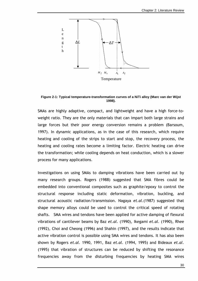
Chapter 2: Literature Review
30
Figure 2-1: Typical temperature-transformation curv es of a NiTi alloy (Marc van der Wijst 1998).
SMAs are highly adaptive, compact, and lightweight and have a high force-to-
weight ratio. They are the only materials that can impart both large strains and
large forces but their poor energy conversion remains a problem (Barsoum,
1997). In dynamic applications, as in the case of this research, which require
heating and cooling of the strips to start and stop, the recovery process, the
heating and cooling rates become a limiting factor. Electric heating can drive
the transformation; while cooling depends on heat conduction, which is a slower
process for many applications.
Investigations on using SMAs to damping vibrations have been carried out by
many research groups. Rogers (1988) suggested that SMA fibres could be
embedded into conventional composites such as graphite/epoxy to control the
structural response including static deformation, vibration, buckling, and
structural acoustic radiation/transmission. Nagaya et.al.(1987) suggested that
shape memory alloys could be used to control the critical speed of rotating
shafts. SMA wires and tendons have been applied for active damping of flexural
vibrations of cantilever beams by Baz et.al. (1990), Ikegami et.al. (1990), Rhee
(1992), Choi and Cheong (1996) and Shahin (1997), and the results indicate that
active vibration control is possible using SMA wires and tendons. It has also been
shown by Rogers et.al. 1990, 1991, Baz et.al. (1994, 1995) and Bideaux et.al.
(1995) that vibration of structures can be reduced by shifting the resonance
frequencies away from the disturbing frequencies by heating SMA wires
L∆ T∆
fM sM fA sA
Temperature
L e n g t h
Chapter 2: Literature Review
31
embedded in a cantilever beam or plate. In this thesis SMA ( in the form of
strips) applications to rotordynamics are introduced, specifically the use of
single-ended and antagonistic active bearing housings, and some prototypical
experiments have given encouraging results for the reduction in the resonant
amplitude for forward whirl in a flexible rotor.
2.9 Piezoelectric Materials
Piezoelectric materials produce electric charge (voltage) if their crystalline
structure is deformed by an external force. This effect is called the direct effect
of piezoelectricity. On the other hand, piezoelectric materials change their
crystalline structure with the application of an external electric field. This
phenomenon is known as the converse effect of piezoelectricity. Pierre and
Jacques Curie discovered the direct effect of piezoelectricity in 1880. The
converse piezoelectric effect was first predicted by Lippmann via methods of
analytical thermodynamics in 1881 which was confirmed by the Curies in 1881.
Thus they can be used both as actuators and sensors (Chopra 2002). Over time
the use of the converse effect of piezoelectricity has become critical in
applications that require oscillators with relatively large amplitude and very
slow rate of decay.
The most commonly used piezoelectric ceramics are barium titanate (BaTiO3),
lead lanthanum zirconate (PLZT), lead magnesium niobate (PMN) and lead
zirconate titanate PZT (PbZrTiO3). These materials exhibit nonlinear coupling
between a mechanical and an electric response. Piezoelectric ceramics can
either be monolithic or made of thin, stacked ceramic layers. They are high-
force, but low stroke devices, have a very broad operating frequency bandwidth,
and exhibit precise positioning response and repeatability. They can achieve
precision that is measured in nanometres (Piezoelectric ceramics- Noliac A/S,
Denmark). One common actuator design, that addresses the limitation in
achievable stroke, is the stack actuator depicted schematically in Figure 2-2.
The stack is created by bonding thin layers of piezoelectric together such that
their polarization directions alternate along the major axis. Electrodes separate
the layers nearly entirely. When a voltage difference is applied across the
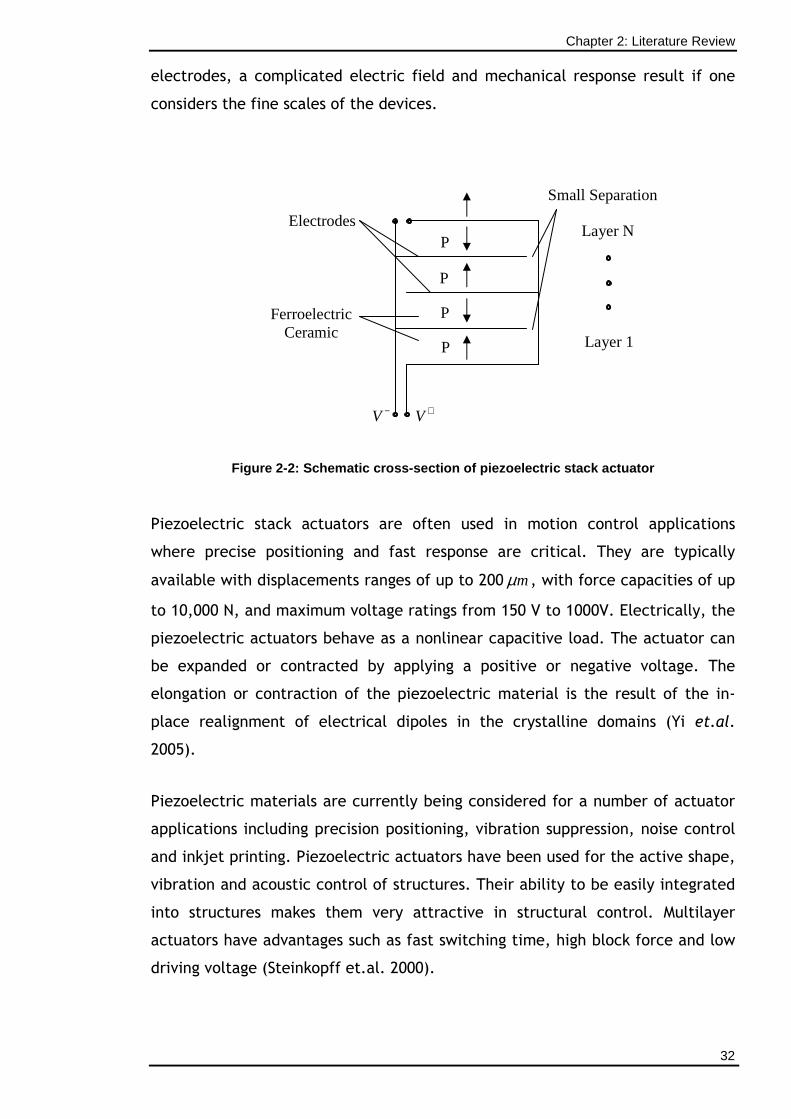
Chapter 2: Literature Review
32
electrodes, a complicated electric field and mechanical response result if one
considers the fine scales of the devices.
Figure 2-2: Schematic cross-section of piezoelectri c stack actuator
Piezoelectric stack actuators are often used in motion control applications
where precise positioning and fast response are critical. They are typically
available with displacements ranges of up to 200 mµ , with force capacities of up
to 10,000 N, and maximum voltage ratings from 150 V to 1000V. Electrically, the
piezoelectric actuators behave as a nonlinear capacitive load. The actuator can
be expanded or contracted by applying a positive or negative voltage. The
elongation or contraction of the piezoelectric material is the result of the in-
place realignment of electrical dipoles in the crystalline domains (Yi et.al.
2005).
Piezoelectric materials are currently being considered for a number of actuator
applications including precision positioning, vibration suppression, noise control
and inkjet printing. Piezoelectric actuators have been used for the active shape,
vibration and acoustic control of structures. Their ability to be easily integrated
into structures makes them very attractive in structural control. Multilayer
actuators have advantages such as fast switching time, high block force and low
driving voltage (Steinkopff et.al. 2000).
V + V −
Electrodes
Ferroelectric Ceramic
Layer 1
Layer N
Small Separation
P
P
P
P
Chapter 2: Literature Review
33
Bailey and Hubbard (1985) introduced piezoelectric actuators to active vibration
control. They used the actuators bonded to the surface of a cantilever beam in
their feedback vibration damping design. Crawley and de Luis (1987) presented
an analytical and experimental development of piezoelectric actuators as
vibration exciters. Using the models they developed from the stress/strain
relationships, they were able to predict the displacement of three real
cantilevered beam and piezoelectric actuator arrangements under steady-state
resonance vibration conditions. Dimitriadis et.al. (1991) had performed a two
dimensional extension of Crawley and de Luis’s work, applying pairs of laminated
piezoelectric actuators to a plate. They demonstrated that the location and
shape of the actuator dramatically affected the vibration response of the plate.
Other researchers such as Fansen and Chen (1986) and Baz and Poh (1988, 1990)
have used piezoelectric actuators in active vibration control experiments,
showing again the potential of piezoelectric actuators as control actuators in
vibration control. The application of piezoelectric stack actuators to control of
vibrations in rotating machinery was considered by Palazzolo et.al. (1989). The
authors showed that significant reductions in the vibration of rotating machinery
could be achieved using two of these actuators in the support structure of the
rotating shaft. In this thesis the author is deliberately introducing parametric
excitations into a flexible rotor by means of a piezoelectric exciter and with the
intention of using this to moderate the responses of the pre-existing mass-
unbalance vibration inherent to the rotor.
Chapter 3: Analytical Modelling of Flexible Rotor Systems
34
CHAPTER 3
ANALYTICAL MODELLING OF FLEXIBLE ROTOR SYSTEMS
_______________________________________________
3.1 Introduction
For several years, a wide variety of phenomena concerning industrial rotor
dynamic systems have been studied and much attention has been given to one
of them, namely the behaviour of rotors under mass unbalance excitation.
One important phenomenon is the self-excited oscillation which has been
shown to be stemming from deviations from assumptions employed such as
linearity. Resonances induced without periodic excitations are called self-
excited oscillations. In the system having a single degree of freedom, the self-
excited oscillation occurs due to the effect of negative damping and the
amplitude grows with time (Kunitoh et.al., (2004)). The dynamic behaviour of
rotors has been extensively studied by Lalanne and Ferraris (1990), Rao
(1991), Ehrich (1992), and Childs (1992). The books by Lalanne and Ferraris
(1990) and Rao (1991) describe the discretisation of the system into
components for the shaft, mass unbalance, bearings and disks. The
mathematical model derived and used in this research is based on the work of
Lalanne and Ferraris (1990). Two models for the equations of motion have
been derived using Lagrangian dynamics and the Rayleigh-Ritz method, and
are used to study some phenomena in rotor systems. The equations of motion
include rotary inertia, gyroscopic coupling, axial load effects and the
influence of nonlinear bearings. Nonlinearities in the system due to inertia
and geometric properties are also considered in the modelling of the
equations of motion. The equations are obtained in the following systematic
way. First the expressions of the kinetic and strain energies of the rotor
elements are constructed and the Rayleigh-Ritz method is applied for the
simplification of the energy expressions. Then, the virtual work of external
forces is modelled and finally Lagrange’s equations are employed to derive
the coupled equations.
Chapter 3: Analytical Modelling of Flexible Rotor Systems
35
3.2 Derivation of the Equations of Motion
In deriving the equations of motion, the scalar method of Lagrangian dynamics
or the vectorial approach of Newtonian mechanics can both be applied to
problems of this sort depending on preference. Lagrangian dynamics permits
the derivation of the equation of motion from three scalar quantities; the
kinetic energy, potential energy, and virtual work of the nonconservative
forces.
The rotor equations are derived by means of the following steps:
Derivation of the kinetic energy of the disk, the shaft and the mass
unbalance. Derivation of strain energy of the shaft. Use of Lagrange’s
equation of the form
iq
i i i i
d T T U WF
dt q q q q
∂ ∂ ∂ ∂− + = = ∂ ∂ ∂ ∂ ɺ (3.2- 1)
where, 1,2i = , T represents the kinetic energy, U is the strain energy, iq are
generalised independent coordinates, and iqF are generalised forces. W∂
represents the virtual work of the nonconservative forces under a virtual
displacement iq∂ .
The Rayleigh-Ritz method has been used to obtain a simple model. It is a
method in which a single function can be replaced by a series of shape
functions multiplied by constant coefficients. It is used for finding the
approximate real resonant frequencies and mode shapes of multi degree of
freedom systems, such as spring mass systems or flywheels on a shaft. In this
work it is used to obtain the displacement functions in terms of the
generalised coordinates for the first mode shape of the shaft with a constant
cross-section in bending that is simply supported at both ends.
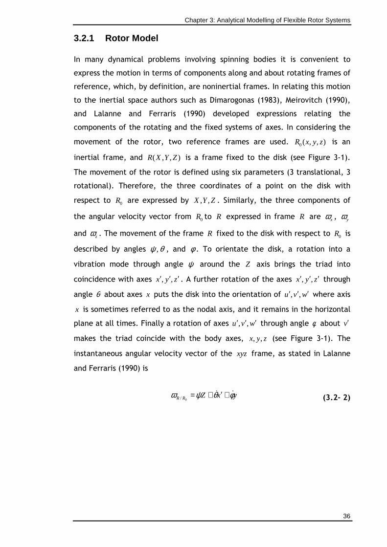
Chapter 3: Analytical Modelling of Flexible Rotor Systems
36
3.2.1 Rotor Model
In many dynamical problems involving spinning bodies it is convenient to
express the motion in terms of components along and about rotating frames of
reference, which, by definition, are noninertial frames. In relating this motion
to the inertial space authors such as Dimarogonas (1983), Meirovitch (1990),
and Lalanne and Ferraris (1990) developed expressions relating the
components of the rotating and the fixed systems of axes. In considering the
movement of the rotor, two reference frames are used. 0( , , )R x y z is an
inertial frame, and ( , , )R X Y Z is a frame fixed to the disk (see Figure 3-1).
The movement of the rotor is defined using six parameters (3 translational, 3
rotational). Therefore, the three coordinates of a point on the disk with
respect to 0R are expressed by , ,X Y Z . Similarly, the three components of
the angular velocity vector from 0R to R expressed in frame R are xω , yω
and zω . The movement of the frame R fixed to the disk with respect to 0R is
described by angles ,ψ θ , and φ . To orientate the disk, a rotation into a
vibration mode through angle ψ around the Z axis brings the triad into
coincidence with axes zyx ′′′ ,, . A further rotation of the axes zyx ′′′ ,, through
angle θ about axes x puts the disk into the orientation of wvu ′′′ ,, where axis
x is sometimes referred to as the nodal axis, and it remains in the horizontal
plane at all times. Finally a rotation of axes wvu ′′′ ,, through angle φ about v′
makes the triad coincide with the body axes, zyx ,, (see Figure 3-1). The
instantaneous angular velocity vector of the xyz frame, as stated in Lalanne
and Ferraris (1990) is
yxZRR φθψω ɺɺɺ +′+=0/ (3.2- 2)
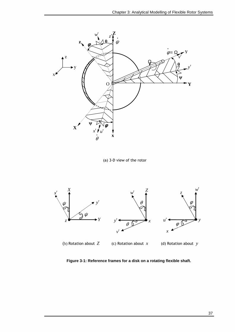
Chapter 3: Analytical Modelling of Flexible Rotor Systems
37
(a) 3-D view of the rotor
(b) Rotation about Z (c) Rotation about x (d) Rotation about y
Figure 3-1: Reference frames for a disk on a rotati ng flexible shaft.
ψ
ψ
z Y
y′
X x′
Z
x
θ
θ
w′
y′
v′
w′
y
φ
φ
z
u′
x
θ
ψ
θ φφφφ
Z
x
Y
X ψ φφφφ
u′ x′
w′ z′ z
O
y′
v′ yφ
•= Ω
Ω
θ•
y
z
ψ•
x
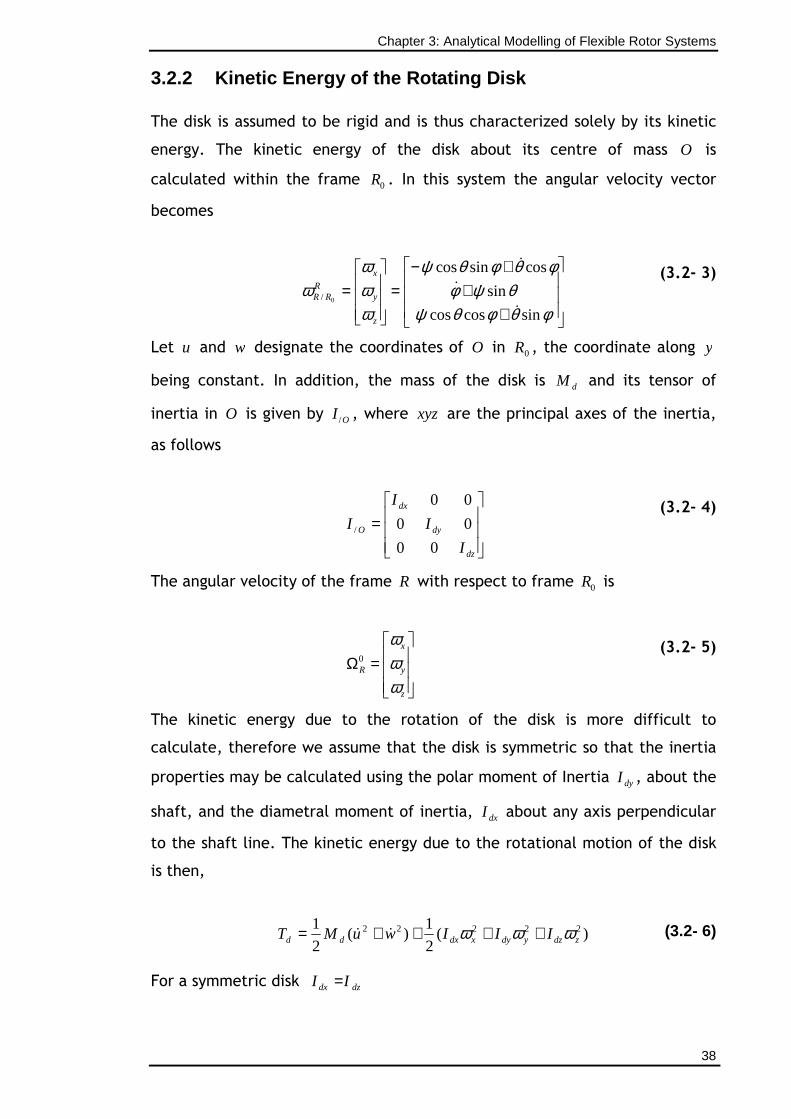
Chapter 3: Analytical Modelling of Flexible Rotor Systems
38
3.2.2 Kinetic Energy of the Rotating Disk
The disk is assumed to be rigid and is thus characterized solely by its kinetic
energy. The kinetic energy of the disk about its centre of mass O is
calculated within the frame 0R . In this system the angular velocity vector
becomes
++
+−=
=φθφθψ
θψφφθφθψ
ωωω
ωsincoscos
sin
cossincos
0/
ɺɺ
ɺɺ
ɺɺ
z
y
xR
RR (3.2- 3)
Let u and w designate the coordinates of O in 0R , the coordinate along y
being constant. In addition, the mass of the disk is dM and its tensor of
inertia in O is given by /OI , where xyz are the principal axes of the inertia,
as follows
=
dz
dy
dx
O
I
I
I
I
00
00
00
/ (3.2- 4)
The angular velocity of the frame R with respect to frame 0R is
0
x
R y
z
ωωω
Ω =
(3.2- 5)
The kinetic energy due to the rotation of the disk is more difficult to
calculate, therefore we assume that the disk is symmetric so that the inertia
properties may be calculated using the polar moment of Inertia dyI , about the
shaft, and the diametral moment of inertia, dxI about any axis perpendicular
to the shaft line. The kinetic energy due to the rotational motion of the disk
is then,
)(
2
1)(
2
1 22222zdzydyxdxdd IIIwuMT ωωω ++++= ɺɺ (3.2- 6)
For a symmetric disk dzdx II =
Chapter 3: Analytical Modelling of Flexible Rotor Systems
39
Substituting the angular velocity vector, equation (3.2-3) into the kinetic
energy of the disk equation (3.2-6) we have
2 2 2 2 2 2 2 21 1 1( ) ( cos ) ( sin 2 sin )
2 2 2d d dx dyT M u w I Iθ ψ θ φ ψ θ φψ θ= + + + + + +ɺ ɺ ɺɺ ɺ ɺɺ ɺ (3.2- 7)
which can be simplified here as the disk is symmetric ( dx dzI I= ), the angles ψ
and θ are small angles, and the angular velocity of the rotor is constant; that
is,
tφ = Ω and φ = Ωɺ (3.2- 8)
Therefore the kinetic energy of the disk becomes,
2 2 2 2 2
2 2 2
1 1( ) ( cos )
2 21
( sin 2 sin )2
d d dx
dy
T M u w I
I
θ ψ θ
ψ θ ψ θ
= + + +
+ Ω + + Ω
ɺ ɺɺ ɺ
ɺ ɺ
(3.2- 9)
where, dM is the mass of the disk and θψ sinɺΩdyI represents the gyroscopic
effect.
3.2.3 Kinetic Energy of the Shaft
The general formulation of the kinetic energy of the shaft is from an
extension of the disk equation (3.2-9). For an element of length l , the
expression for the kinetic energy is,
( ) ( )
( )
2 2 2 2 2 2
0 0
2 2
0 0
cos2 2
( sin ) 2 sin2
l l
s
l l
s IT u w dy dy IL
Idy I dy
ρ ρ θ ψ θ ρ
ρ ψ θ ρ ψ θ
= + + + + Ω
+ + Ω
∫ ∫
∫ ∫
ɺ ɺɺ ɺ
ɺ ɺ
(3.2- 10)
where, ρ is mass per unit volume, S is the cross-sectional area of the shaft,
I is area moment of Inertia of the shaft cross-section about the neutral axis ,
dy is the thickness of the shaft, ( )dywus l
∫ +02
ɺɺρ
is the classical expression for
the kinetic energy of the shaft in bending, ( )dyI l
∫ +0
222 cos2
θψθρɺɺ is the
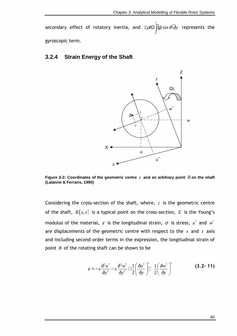
Chapter 3: Analytical Modelling of Flexible Rotor Systems
40
secondary effect of rotatory inertia, and ( )∫Ωl
dyI0
sin2 θψρ ɺ represents the
gyroscopic term.
3.2.4 Strain Energy of the Shaft
Figure 3-2: Coordinates of the geometric centre c and an arbitrary point B on the shaft (Lalanne & Ferraris, 1990)
Considering the cross-section of the shaft, where, c is the geometric centre
of the shaft, ( ),B x z is a typical point on the cross-section, E is the Young’s
modulus of the material, ε is the longitudinal strain, σ is stress, *u and *w
are displacements of the geometric centre with respect to the x and z axis
and including second–order terms in the expression, the longitudinal strain of
point B of the rotating shaft can be shown to be
2 22 * 2 * * *
2 2
1 1
2 2
u w u wx z
y y y yε ∂ ∂ ∂ ∂= − − + + ∂ ∂ ∂ ∂
(3.2- 11)
x
Z
X
z
*u
*w
w
u
c B
tΩ
z
x
Chapter 3: Analytical Modelling of Flexible Rotor Systems
41
Let 2 * 2 *
2 2l
u wx z
y yε ∂ ∂= − −
∂ ∂ (3.2- 12)
and 2 2* *1 1
2 2nl
u w
y yε ∂ ∂= + ∂ ∂
(3.2- 13)
where, lε contains the linear strain terms and nlε contains the nonlinear
strain terms. Thus equation (3.2-11) can be written as
l nlε ε ε= + (3.2- 14)
The strain energy of the shaft is
1
1
2 τ
εσ τ= ∫U d (3.2- 15)
where τ is the volume of the shaft and the relationship between stress and
strain is
Eσ ε= (3.2- 16)
Substituting equations (3.2-14) and (3.2-16) into the strain energy equation
(3.2-15) we get,
( )2 21 2
2 l l nl nl
EU d
τ
ε ε ε ε τ= + +∫ (3.2- 17)
The second integral in equation (3.2-17) gives rise to a stiffness term, which
couples the linear and nonlinear strains. It is assumed that the cross-section
of the shaft is circular, and the arbitrary point B will be symmetrical about
the axes x and z , thus making the shaft cross-section with respect to x and
z symmetrical. The symmetry of the shaft cross-section with respect to x
and z results in the second term being
0nl ldτ
ε ε τ =∫ (3.2- 18)
Chapter 3: Analytical Modelling of Flexible Rotor Systems
42
The strain energy therefore becomes,
22 2 22 * 2 * * *
1 2 20
1 1
2 2 2
l
s
E u w u wU x z dSdy
y y y y
∂ ∂ ∂ ∂ = − − + + ∂ ∂ ∂ ∂
∫ ∫ (3.2- 19)
Expanding equation (3.2-19) gives,
2 22 * 2 * 2 * 2 *2 2
2 2 2 2
1 4 2 2 4* * * *0
2
2 1 1 1
4 2 4
l
s
u w u wx z xz
y y y yEU dSdy
u u w w
y y y y
∂ ∂ ∂ ∂ + + ∂ ∂ ∂ ∂ =
∂ ∂ ∂ ∂+ + + ∂ ∂ ∂ ∂
∫ ∫ (3.2- 20)
Because of symmetry, the integral of the third term in equation (3.2-20) is
equal to zero. Introducing area moments of Inertia with respect to x and z
2x
s
I z ds= ∫ (3.2- 21)
2z
s
I x ds= ∫ (3.2- 22)
where s is the cross-sectional area. The strain energy expression is thus
2 22 * 2 *
1 2 202
l
z x
E u wU I I dy
y y
∂ ∂ = + ∂ ∂ ∫
(3.2- 23)
If the shaft is subjected to a constant axial force 0F there is a further
contribution to the strain energy of the shaft given by
( )0
2
0
l
l nl
FU d
sε ε τ= +∫ (3.2- 24)
Owing to symmetry, the first term under the integral will vanish over the
cross-sectional area; substituting equations (3.2-12) and (3.2-13) into
equation (3.2-24) gives
2 2* *0
2
02
lF u wU dy
y y
∂ ∂ = + ∂ ∂ ∫
(3.2- 25)
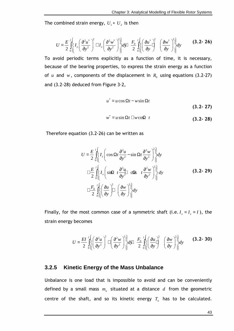
Chapter 3: Analytical Modelling of Flexible Rotor Systems
43
The combined strain energy, 1U + 2U is then
2 2 2 22 * 2 * * *0
2 20 02 2
l l
z x
FE u w u wU I I dy dy
y y y y
∂ ∂ ∂ ∂ = + + + ∂ ∂ ∂ ∂ ∫ ∫
(3.2- 26)
To avoid periodic terms explicitly as a function of time, it is necessary,
because of the bearing properties, to express the strain energy as a function
of u and w , components of the displacement in 0R using equations (3.2-27)
and (3.2-28) deduced from Figure 3-2,
* cos sinu u t w t= Ω − Ω (3.2- 27)
* sin cosw u t w t= Ω + Ω (3.2- 28)
Therefore equation (3.2-26) can be written as
22 2
2 20
22 2
2 20
2 2
0
0
cos sin2
sin cos2
2
l
z
l
x
l
E u wU I t t dy
y y
E u wI t t dy
y y
F u wdy
y y
∂ ∂ = Ω − Ω ∂ ∂
∂ ∂ + Ω + Ω ∂ ∂
∂ ∂ + + ∂ ∂
∫
∫
∫
(3.2- 29)
Finally, for the most common case of a symmetric shaft (i.e. x zI I I= = ), the
strain energy becomes
2 2 2 22 20
2 20 02 2
l lFEI u w u wU dy dy
y y y y
∂ ∂ ∂ ∂ = + + + ∂ ∂ ∂ ∂ ∫ ∫
(3.2- 30)
3.2.5 Kinetic Energy of the Mass Unbalance
Unbalance is one load that is impossible to avoid and can be conveniently
defined by a small mass um situated at a distance d from the geometric
centre of the shaft, and so its kinetic energy uT has to be calculated.
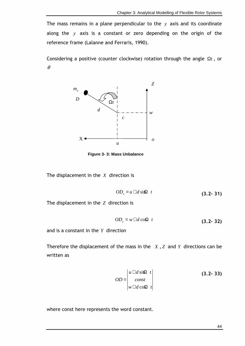
Chapter 3: Analytical Modelling of Flexible Rotor Systems
44
The mass remains in a plane perpendicular to the y axis and its coordinate
along the y axis is a constant or zero depending on the origin of the
reference frame (Lalanne and Ferraris, 1990).
Considering a positive (counter clockwise) rotation through the angle tΩ , or
θ
Z
Figure 3- 3: Ma ss Unbalance
The displacement in the X direction is
sinxOD u d t= + Ω (3.2- 31)
The displacement in the Z direction is
cosyOD w d t= + Ω (3.2- 32)
and is a constant in the Y direction
Therefore the displacement of the mass in the X , Z and Y directions can be
written as
sin
cos
u d t
OD const
w d t
+ Ω=
+ Ω
(3.2- 33)
where const here represents the word constant.
c
o u
d
D tΩ
um
w
X
Chapter 3: Analytical Modelling of Flexible Rotor Systems
45
Then velocity can be stated as
cos( )
0
sin
u d td OD
Vdt
w d t
+ Ω Ω= =
− Ω Ω
ɺ
ɺ
(3.2- 34)
and the kinetic energy of the mass unbalance is
( )tdwtuddwum
T uu ΩΩ−ΩΩ+Ω++= sin2cos2
22222
ɺɺɺɺ (3.2- 35)
The term 2/22dmu Ω is a constant in this context and has no subsequent
influence on the equations. The mass unbalance um is smaller than the mass
of the rotor, so the expression for the kinetic energy can be written as
( )twtudmT uu Ω−ΩΩ≅ sincos ɺɺ (3.2- 36)
3.2.6 Simplified Model
The Rayleigh-Ritz method is used to study a model composed of a shaft of
length l , supporting a disk located at 1l along the shaft (see Figure 3-4). It is
used to devise new expressions for the displacement in the x and z
directions in terms of the generalised coordinates. The rotor is assumed to be
simply supported at both ends and neglecting the argument t for simplicity,
the expression for the displacement in the x and z directions are
( ) 11 )()()(, qyftqyftyu == (3.2- 37)
( ) 22 )()()(, qyftqyftyw == (3.2- 38)
where, 1q and 2q are generalised independent coordinates and ( )f y is the
displacement function, and it is chosen as the normalised first mode shape of
a beam with a constant cross section in bending and simply supported at both
ends, and is given as
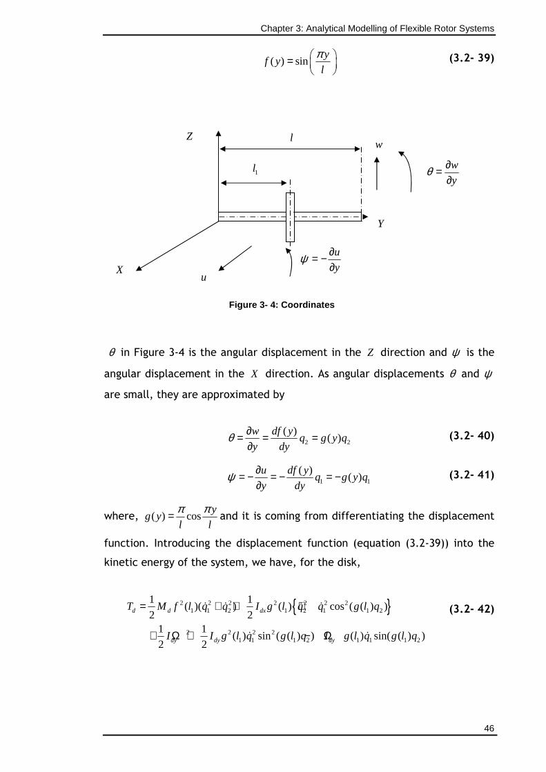
Chapter 3: Analytical Modelling of Flexible Rotor Systems
46
( ) sin
yf y
l
π =
(3.2- 39)
Figure 3- 4: Coordinates
θ in Figure 3-4 is the angular displacement in the Z direction and ψ is the
angular displacement in the X direction. As angular displacements θ and ψ
are small, they are approximated by
2 2
( )( )
w df yq g y q
y dyθ ∂= = =
∂ (3.2- 40)
1 1
( )( )
u df yq g y q
y dyψ ∂= − = − = −
∂ (3.2- 41)
where, ( ) cosy
g yl l
π π= and it is coming from differentiating the displacement
function. Introducing the displacement function (equation (3.2-39)) into the
kinetic energy of the system, we have, for the disk,
2 2 2 2 2 2 21 1 2 1 2 1 1 2
2 2 2 21 1 1 2 1 1 1 2
1 1( )( ) ( ) cos ( ( ) )
2 21 1
( ) sin ( ( ) ) ( ) sin( ( ) )2 2
d d dx
dy dy dy
T M f l q q I g l q q g l q
I I g l q g l q I g l q g l q
= + + +
+ Ω + − Ω
ɺ ɺ ɺ ɺ
ɺ ɺ
(3.2- 42)
y
w
∂∂=θ
Z
X
Y
w
u y
u
∂∂−=ψ
l
1l
Chapter 3: Analytical Modelling of Flexible Rotor Systems
47
For the shaft
( ) ( )
( )
2 2 2 2 2 2 21 2 2 1 1 2
0 0
2 2 2 21 1 2 1 1 2
0 0
( ) cos ( ( ) )2 2
( ) sin ( ( ) ) 2 sin( ( ) )2
l l
s
l l
s IT f y dy q q g y dy q q g l q
IIL g y dy q g l q I g y dyq g l q
ρ ρ
ρρ ρ
= + + +
+ Ω + − Ω
∫ ∫
∫ ∫
ɺ ɺ ɺ
ɺ ɺ
(3.2- 43)
For the disk and shaft combined
( ) ( )
2 2 2 21 1 2
0
2 2 2 2 21 2 1 1 2
0
2 2 2 2 21 1 1 2
0
1 1 1 2
0
1( )
2
1( ) ( ) cos ( ( ) )
2
1 1( ) ( ) sin ( ( ) )
2 2
( ) 2 ( ) sin( ( )
l
d
l
dx
l
dy dy
l
dy
T M f l s f y dy q q
I g l I g y dy q q g l q
I IL I g l I g y dy q g l q
I g l I g y dy q g l q
ρ
ρ
ρ ρ
ρ
= + +
+ + +
+ Ω + + +
− Ω +
∫
∫
∫
∫
ɺ ɺ
ɺ ɺ
ɺ
ɺ )
(3.2- 44)
Simplifying equation (3.2-44) gives
( ) ( )( )2 2 21 2 2 1 2
1 1sin
2 2 dyT m q q I IL a q qρ = + + Ω + − Ω ϒ
ɺ ɺ ɺ (3.2- 45)
where,
1( )g lϒ = , 1m m P= + , ( ) ( )2 21 1
0
l
dm M f l s f y dyρ= + ∫ , ( ) ( )2 21
0
l
dxP I g l I g y dyρ= + ∫ ,
dx dyI I≈ , ( ) ( )∫+=l
dy dyygIlgIa0
12 2ρ , 11( ) sin
lf l
l
π =
, and 11( ) cos
lg l
l l
ππ= . 1l
and l values are obtained from the experimental rig.
Also introducing the displacement function (equation (3.2-39)) into the kinetic
energy of the mass unbalance expression of equation (3.2-36) gives
( )( )tqtqldfmT uu Ω−ΩΩ= sincos 211 ɺɺ (3.2- 46)
Likewise, introducing this displacement function into the strain energy of the
shaft results in,
Chapter 3: Analytical Modelling of Flexible Rotor Systems
48
( ) ( )2 2 2 2 2 20
1 2 1 2
0 0
( ) ( )2 2
l lFEIU h y dy q q g y dy q q= + + +∫ ∫ (3.2- 47)
where, 2
2
( )( )
d f yh y
dy= . Simplifying equation (3.2-47) gives
( )2 21 2
1
2 sU k q q= + (3.2- 48)
where, 2 20
0 0
( ) ( )l l
sk EI h y dy F g y dy= +∫ ∫ and is the stiffness of the shaft .
Equations (3.2-45), (3.2-46) and (3.2-48) are the kinetic energy expression for
the disk and shaft combined, the kinetic energy expression for the mass
unbalance and the strain energy expression for the shaft respectively, in
terms of the generalised coordinates.
3.2.7 Nonlinear Bearing
In rotating machinery, the dynamic stiffness of the bearing which supports the
rotating shaft can have a significant quantitative and qualitative effect on the
vibration within the machine. In particular it affects the machine critical
speeds and the vibration in between critical speeds. Rolling bearings
sometimes have nonlinear spring characteristics due to Coulomb friction and
the angular clearance between roller and ring (An-Chen et.al.1993). Brown
et.al.(1994) assuming linear damping force and using short bearing theory
verified that a simple model of a rigidly supported hydrodynamic journal
bearing can be shown to behave chaotically when the rotating unbalance
force exceeds the gravitational load. Chen et.al. (1998) in the study of chaos
in the unbalanced response of a flexible rotor supported by oil film bearings
with nonlinear suspension assumed a linear damping force and their findings
showed that the dimension of the bearing centre trajectory is fractal and
greater than two in some operating conditions, indicating that the system is in
a state of chaotic motion. For simplification, the damping forces of the
bearing are assumed to be linear. Thus, the equations of the bearing forces as
shown in Figure 3-5 are expressed in the following.
Chapter 3: Analytical Modelling of Flexible Rotor Systems
49
n nx xx xz xx xz xx xzF k x k z k x k z C x C z= + + + + +ɺ ɺ (3.2- 49)
n nz zx zz zx zz zx zzF k x k z k x k z C x C z= + + + + +ɺ ɺ (3.2- 50)
where, 1,2...n = ,
ijk are linear spring coefficients; zxji ,, =
ijk are nonlinear spring coefficients; zxji ,, =
ijC are linear damping coefficients; zxji ,, =
In practice, all components of these nonlinear forces appear markedly up to
the third power of deflections in single-row ball bearings (Yamamoto
et.al.1981). Therefore, the bearing is assumed to have cubic nonlinear spring,
and linear damping characteristics is also assumed. The generalised force
from the bearing can be written as
x zF F F= + (3.2- 51)
The virtual work associated with a generalised force is
i iq q iW F qδ δ = (3.2- 52)
where the generalised force iqF is associated with the generalised coordinate
iq . Taking u and w as lateral displacements of the centre of mass of the disk
with respect to the fixed frame , ,X Y Z , then the virtual work, which is the
sum of the virtual work terms for the damping and stiffness effects of the
bearing, can be expressed if u u uδ→ + and 0wδ = , to give
( ) [ ] [ ]
[ ] [ ]
3
3
xx xz xxu
xz xx xz
W k u u k w u k u u
k w u c u u c w u
δ δ δ δ
δ δ δ
= − + − + −
+ − + − + − ɺ ɺ
(3.2- 53)
For the case where w w wδ→ + and 0uδ = , then,
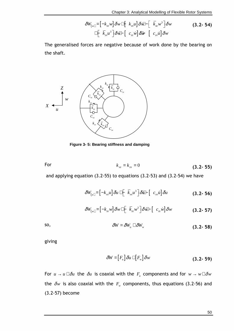
Chapter 3: Analytical Modelling of Flexible Rotor Systems
50
( ) [ ] [ ]
[ ] [ ]
3
3
zz zx zzw
zx zz zx
W k w w k u w k w w
k u w c w w c u w
δ δ δ δ
δ δ δ
= − + − + −
+ − + − + − ɺ ɺ
(3.2- 54)
The generalised forces are negative because of work done by the bearing on
the shaft.
Figure 3- 5: Bearing stiffne ss and damping
For 0== zxxz kk (3.2- 55)
and applying equation (3.2-55) to equations (3.2-53) and (3.2-54) we have
( ) [ ] [ ]3
xx xx xxuW k u u k u u c u uδ δ δ δ = − + − + − ɺ (3.2- 56)
( ) [ ] [ ]3
zz zz zzwW k w w k w w c w wδ δ δ δ = − + − + − ɺ (3.2- 57)
so, u wW W Wδ δ δ= + (3.2- 58)
giving
[ ] [ ]u wW F u F wδ δ δ= + (3.2- 59)
For u u uδ→ + the uδ is coaxial with the uF components and for w w wδ→ +
the wδ is also coaxial with the wF components, thus equations (3.2-56) and
(3.2-57) become
X
Z
u
w
xzk zzC
zzk zzk
xzk xzC
xxC
zxk
xxk
zxC zxk
zxk
Chapter 3: Analytical Modelling of Flexible Rotor Systems
51
3u xx xxF k x k x Cx= − − − ɺ (3.2- 60)
3w zz zzF k z k z Cz= − − − ɺ (3.2- 61)
Applying equations (3.2-37) and (3.2-38) to (3.2-60) and (3.2-61) we have,
( ) ( ) ( )1
3
2 1 2 1 2 1q xx xx xxF k f l q k f l q C f l q = − − − ɺ (3.2- 62)
( ) ( ) ( )2
3
2 2 2 2 2 2q zz zz zzF k f l q k f l q C f l q = − − − ɺ (3.2- 63)
For a symmetrical bearing
)()()( 222 lkflfklfk zzxx == (3.2- 64)
3 3 32 2 2( ) ( ) ( )xx zzk f l k f l kf l= = (3.2- 65)
)()()( 222 lfClfClfC bzzxx == (3.2- 66)
Then, letting,
( )2 bkf l k= (3.2- 67)
( )32kf l b= (3.2- 68)
2( )b bC f l c= (3.2- 69)
where, bk is the bearing stiffness coefficient and bc is the bearing damping
coefficient. Substituting equations (3.2-64) to (3.2-69) into equations (3.2-62)
and (3.2-63) we obtain
Chapter 3: Analytical Modelling of Flexible Rotor Systems
52
1
3111
qcbqqkF bbq ɺ−−−= (3.2- 70)
2
3222
qcbqqkF bbq ɺ−−−= (3.2- 71)
where; 1qF and
2qF are the two components of the force.
The Smart Actuator introduces a Y directed axial force component into the
bearing force. This is a force vF directed along Y when switched on, and
therefore the virtual work expression of equation (3.2-59) extends to
[ ] [ ] [ ]u w vW F u F w F vδ δ δ δ= + + (3.2- 72)
vF is assumed to be positive because it is external. Therefore expressing vF in
terms of 1q and 2q we have 1
1qv actF F q= and 2
2qv actF F q= respectively. Where,
actF is the actuator force. (See Appendix A-1 for the derivation of the actuator
force term). For v v vδ→ + , the vδ is coaxial with the vF components, so the
two components of the forces extend to
1
31 1 1 1q b b actF k q bq c q F q= − − − +ɺ (3.2- 73)
2
32 2 2 2q b b actF k q bq c q F q= − − − +ɺ (3.2- 74)
3.2.8 Equations of Motion
Now applying Lagrange’s equations (3.2.1) to the kinetic energy given by the
addition of (3.2-45) and (3.2-46) and the strain energy given by (3.2-48) and
using 1q and 2q as generalised coordinates and the generalised forces as
1qF and 2qF results in the equations in the following subsections.
Chapter 3: Analytical Modelling of Flexible Rotor Systems
53
3.2.8.1 Alternative Analytical Model A
In this model large deflections are accommodated within the equations.
( ) 3 21 5 2 2 1 1 1 1 sinb act umq a q Cos q kq bq c q F q m d t− Ω ϒ + + + − = Ω Ωɺɺ ɺ ɺ (3.2- 75)
( ) 3 22 5 1 2 2 2 2 2 cosb act umq a q Cos q kq bq c q F q m d t+ Ω ϒ + + + − = Ω Ωɺɺ ɺ ɺ (3.2- 76)
where; bs kkk += ; 5 2a a= ϒ , ( )1 1.325g lϒ = = , this is calculated using data from
the experimental rig, and k is the rotor-bearing radial stiffness representing
the combined circumferentially-symmetric stiffness of the rotor shaft and
bearings.
Reference to Appendix A-2 provides a discussion of the equations (3.2-75) and
(3.2-76).
3.2.8.2 Alternative Analytical Model B
Going back to the kinetic energy expression equation (3.2-45) and applying
small angle approximation of the form sinθ θ≈ and cos 1θ ≈ , leads to
( ) ( )2 2 21 2 2 1 2
1 1
2 2 dyT m q q I IL a q qρ = + + Ω + − Ω ϒ
ɺ ɺ ɺ (3.2- 77)
Thus equation (3.2-77) becomes
( )2 2 21 2 5 1 2
1 1
2 2 dyT m q q I IL a q qρ = + + Ω + − Ω
ɺ ɺ ɺ (3.2- 78)
Applying Lagrange’s equations (3.2-1) to the kinetic energy given by the
addition of (3.2-78) and (3.2-46) and the strain energy given by (3.2-48) gives
the equations
3 21 5 2 1 1 1 1 sinb act umq a q kq bq c q F q m d t− Ω + + + − = Ω Ωɺɺ ɺ ɺ (3.2- 79)
3 22 5 1 2 2 2 2 cosb act umq a q kq bq c q F q m d t+ Ω + + + − = Ω Ωɺɺ ɺ ɺ (3.2- 80)
Chapter 3: Analytical Modelling of Flexible Rotor Systems
54
3.2.8.3 Alternative Analytical Model C
Taking a small angle approximation to the Model A equations, using the
Maclaurin Series in the form 3 52 2
2 2 ...3! 5!
q qsin q q= − + − + and
2 42 2
2 1 ...2! 4!
q qcos q = − + − + to expand the trigonometrical functions in equations
(3.2-75) and (3.2-76) by assuming the flexible rotor lateral oscillations to be
finite, but not very large, and for small angles of 2q , the expansions of sin 2q
and cos 2q will be dominated by the leading term. Thus for small vibrations we
can make the approximation of replacing ( )2sin qϒ by ( )2qϒ and ( )2cos qϒ by
1, equations (3.2-75) and (3.2-76) therefore become,
3 21 5 2 1 1 1 1 sinb act umq a q kq bq c q F q m d t− Ω + + + − = Ω Ωɺɺ ɺ ɺ (3.2- 81)
3 22 5 1 2 2 2 2 cosb act umq a q kq bq c q F q m d t+ Ω + + + − = Ω Ωɺɺ ɺ ɺ (3.2- 82)
3.2.9 Linear Viscous Damping
Damping is a nonlinear phenomenon and some examples are hysteretic
damping, Coulomb dry friction and aerodynamic drag. Linear viscous damping
is an idealisation, which provides a term proportional to velocity. Including
linear viscous term ( qcs ɺ ) into equations (3.2-75), (3.2-76), (3.2-79), (3.2-80),
(3.2-81) and (3.2-82) we get the three equation models as,
3.2.9.1 Model A
( ) 3 21 1 5 2 2 1 1 1 sinact umq cq a q Cos q kq bq F q m d t+ − Ω ϒ + + − = Ω Ωɺɺ ɺ ɺ (3.2- 83)
( ) 3 22 2 5 1 2 2 2 2 cosact umq cq a q Cos q kq bq F q m d t+ + Ω ϒ + + − = Ω Ωɺɺ ɺ ɺ (3.2- 84)
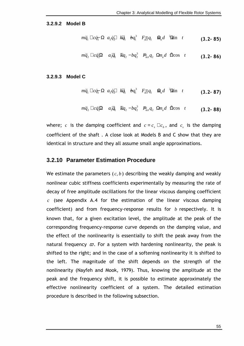
Chapter 3: Analytical Modelling of Flexible Rotor Systems
55
3.2.9.2 Model B
3 21 1 5 2 1 1 1 sinact umq cq a q kq bq F q m d t+ − Ω + + − = Ω Ωɺɺ ɺ ɺ (3.2- 85)
3 22 2 5 1 2 2 2 cosact umq cq a q kq bq F q m d t+ + Ω + + − = Ω Ωɺɺ ɺ ɺ (3.2- 86)
3.2.9.3 Model C
3 21 1 5 2 1 1 1 sinact umq cq a q kq bq F q m d t+ − Ω + + − = Ω Ωɺɺ ɺ ɺ (3.2- 87)
3 22 2 5 1 2 2 2 cosact umq cq a q kq bq F q m d t+ + Ω + + − = Ω Ωɺɺ ɺ ɺ (3.2- 88)
where; c is the damping coefficient and bs ccc += , and sc is the damping
coefficient of the shaft . A close look at Models B and C show that they are
identical in structure and they all assume small angle approximations.
3.2.10 Parameter Estimation Procedure
We estimate the parameters ( ,c b ) describing the weakly damping and weakly
nonlinear cubic stiffness coefficients experimentally by measuring the rate of
decay of free amplitude oscillations for the linear viscous damping coefficient
c (see Appendix A.4 for the estimation of the linear viscous damping
coefficient) and from frequency-response results for b respectively. It is
known that, for a given excitation level, the amplitude at the peak of the
corresponding frequency-response curve depends on the damping value, and
the effect of the nonlinearity is essentially to shift the peak away from the
natural frequency ω . For a system with hardening nonlinearity, the peak is
shifted to the right; and in the case of a softening nonlinearity it is shifted to
the left. The magnitude of the shift depends on the strength of the
nonlinearity (Nayfeh and Mook, 1979). Thus, knowing the amplitude at the
peak and the frequency shift, it is possible to estimate approximately the
effective nonlinearity coefficient of a system. The detailed estimation
procedure is described in the following subsection.
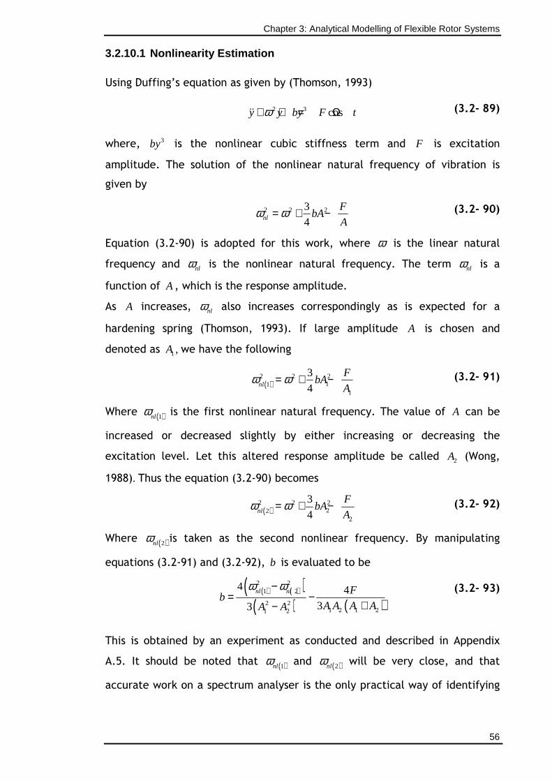
Chapter 3: Analytical Modelling of Flexible Rotor Systems
56
3.2.10.1 Nonlinearity Estimation
Using Duffing’s equation as given by (Thomson, 1993)
2 3 cosy y by F tω+ + = Ωɺɺ (3.2- 89)
where, 3by is the nonlinear cubic stiffness term and F is excitation
amplitude. The solution of the nonlinear natural frequency of vibration is
given by
2 2 23
4nl
FbA
Aω ω= + − (3.2- 90)
Equation (3.2-90) is adopted for this work, where ω is the linear natural
frequency and nlω is the nonlinear natural frequency. The term nlω is a
function of A , which is the response amplitude.
As A increases, nlω also increases correspondingly as is expected for a
hardening spring (Thomson, 1993). If large amplitude A is chosen and
denoted as 1A , we have the following
( )
2 2 211
1
3
4nl
FbA
Aω ω= + − (3.2- 91)
Where ( )1nlω is the first nonlinear natural frequency. The value of A can be
increased or decreased slightly by either increasing or decreasing the
excitation level. Let this altered response amplitude be called 2A (Wong,
1988). Thus the equation (3.2-90) becomes
( )
2 2 222
2
3
4nl
FbA
Aω ω= + − (3.2- 92)
Where ( )2nlω is taken as the second nonlinear frequency. By manipulating
equations (3.2-91) and (3.2-92), b is evaluated to be
( ) ( )( )
( ) ( )
2 21 2
2 21 2 1 21 2
4 4
33
nl nl Fb
A A A AA A
ω ω−= −
+−
(3.2- 93)
This is obtained by an experiment as conducted and described in Appendix
A.5. It should be noted that ( )1nlω and ( )2nlω will be very close, and that
accurate work on a spectrum analyser is the only practical way of identifying
Chapter 3: Analytical Modelling of Flexible Rotor Systems
57
this shift as the response amplitude itself shifts from 1A to 2A during the small
change introduced by shifting the excitation amplitude level.
3.2.11 Discussions
A rotor system can be considered a vibrating system in the classical sense. It
is represented by a system of equations which relates excitations and
responses, where responses of interest are motions of the geometric centre of
the shaft. Excitations can be due to rotating mass unbalance. A resonance
condition exists when the frequency of excitation due to mass unbalance
coincides with the natural frequency. The rotating system has several unique
features compared to other vibrating systems due to its rotation. Mass
unbalance provides excitation which is present whenever the rotor spins; for
this reason mass unbalance is considered an integral part of the analysis as
opposed to an excitation term. The tendency of a rotor disk’s angular
momentum or the momentum of the rotor itself, to couple with rotations
about the bearing is called the “gyroscopic effect” and causes the natural
frequencies to vary with rotor speed. Equations of the rotor system are
obtained systematically in the following way. First the expressions of the disk
kinetic, shaft kinetic, mass unbalance kinetic and strain energies of the rotor
elements are constructed. Then the virtual work of external forces, including,
bearing and axial force terms are formed. The axial force term enables one to
include or apply an external force axially into the rotor system. A numerical
method, Rayleigh-Ritz method which gives simple models that are useful to
understanding of the basic phenomena, has been used to simplify the model.
Lagrange’s equations are applied to the expressions, firstly by accommodating
large deflections to obtain the model A equations, and secondly, by making
small angle approximations to obtain the model B and C equations.
Chapter 4: Approximate Analytical and Numerical Solutions to the Equations of Motion
58
CHAPTER 4
APPROXIMATE ANALYTICAL AND NUMERICAL SOLUTIONS TO THE EQUATIONS OF MOTION
__________________________________________
4.1 Introduction
In this chapter nonlinear vibrations of the flexible rotor while passing through
primary resonance and the associated stability behaviour are analysed, with and
without an axial parametric excitation. Solutions are developed based on an
appropriate Jeffcott rotor model, which consists of a single unbalanced disk
attached to an elastic shaft at mid-span. The classical perturbation Method of
Multiple Scales (MMS) has been chosen for the analysis of the equations of
motion because the solution is a function of multiple independent time-scales,
so the fast scale can be used for capturing motions at frequencies comparable to
the linear frequency of the system, whilst the slow scale accounts for slow
modulations of amplitudes and phases. This method is well discussed in the
books of Nayfeh and Mook (1979), Cartmell (1990), and Murdock (1999). Cartmell
et.al. (2003) reviewed the Multiple Scales Method as applied to the weakly
nonlinear dynamics of mechanical systems. The MMS is one of several tools used
to study the nonlinear equations of motion and is sometimes suitable for solving
stability problems. The principal difference between this and other perturbation
methods is that the time (independent variable) is represented by independent
time scales. Its chief advantage over other perturbation techniques, such as the
Lindstedt-Poincaré method, is that it is easily applicable to damped systems. It
also generates all possible resonance conditions and allows the user great
control over the overall accuracy of the solution (Cartmell,1984). The underlying
idea of this method is to consider an expansion of the dependent variables as a
function of multiple independent variables, or scales, instead of a single
independent variable. Extended expansions based on “slow” and “fast” time
scales are applied to obtain uniform expansions for the amplitudes of the
motion. Expressions for the amplitude and phase modulation functions are
explicitly obtained, and manipulated to yield steady-state solutions. Frequency-
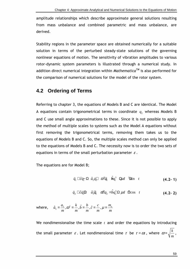
Chapter 4: Approximate Analytical and Numerical Solutions to the Equations of Motion
59
amplitude relationships which describe approximate general solutions resulting
from mass unbalance and combined parametric and mass unbalance, are
derived.
Stability regions in the parameter space are obtained numerically for a suitable
solution in terms of the perturbed steady-state solutions of the governing
nonlinear equations of motion. The sensitivity of vibration amplitudes to various
rotor-dynamic system parameters is illustrated through a numerical study. In
addition direct numerical integration within MathematicaTM is also performed for
the comparison of numerical solutions for the model of the rotor system.
4.2 Ordering of Terms
Referring to chapter 3, the equations of Models B and C are identical. The Model
A equations contain trigonometrical terms in coordinate 2q whereas Models B
and C use small angle approximations to these. Since it is not possible to apply
the method of multiple scales to systems such as the Model A equations without
first removing the trigonometrical terms, removing them takes us to the
equations of Models B and C. So, the multiple scales method can only be applied
to the equations of Models B and C. The necessity now is to order the two sets of
equations in terms of the small perturbation parameter ε .
The equations are for Model B;
2 3 21 1 5 2 1 1
ˆˆ ˆ sinq cq a q q bq d tω µ+ − Ω + + = Ω Ωɺɺ ɺ ɺ (4.2- 1)
2 3 22 2 5 1 2 2
ˆˆ ˆ cosq cq a q q bq d tω µ+ + Ω + + = Ω Ωɺɺ ɺ ɺ (4.2- 2)
where, 255
ˆˆ ˆ, , , , ua mk b ca b c
m m m m mω µ= = = = =
We nondimensionalise the time scale t and order the equations by introducing
the small parameter ε . Let nondimensional time τ be tτ ω= , where k
mω = ,
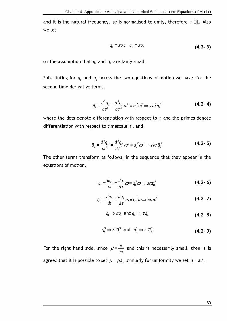
Chapter 4: Approximate Analytical and Numerical Solutions to the Equations of Motion
60
and it is the natural frequency. ω is normalised to unity, therefore 1τ ≅ . Also
we let
1 1 2 2;q q q qε ε= = (4.2- 3)
on the assumption that 1q and 2q are fairly small.
Substituting for 1q and 2q across the two equations of motion we have, for the
second time derivative terms,
2 22 2 21 1
1 1 12 2
d q d qq q q
dt dω ω εω
τ′′ ′′= = ≡ ⇒ɺɺ (4.2- 4)
where the dots denote differentiation with respect to t and the primes denote
differentiation with respect to timescale τ , and
2 22 2 22 2
2 2 22 2
d q d qq q q
dt dω ω εω
τ′′ ′′= = ≡ ⇒ɺɺ (4.2- 5)
The other terms transform as follows, in the sequence that they appear in the
equations of motion,
1 11 1 1
dq dqq q q
dt dω ω εω
τ′ ′= = ≡ ⇒ɺ (4.2- 6)
2 22 2 2
dq dqq q q
dt dω ω εω
τ′ ′= = ≡ ⇒ɺ (4.2- 7)
1 1q qε⇒ and 2 2q qε⇒ (4.2- 8)
3 3 31 1q qε⇒ and 3 3 3
2 2q qε⇒ (4.2- 9)
For the right hand side, since um
mµ = and this is necessarily small, then it is
agreed that it is possible to set µ µε= ; similarly for uniformity we set d dε= .
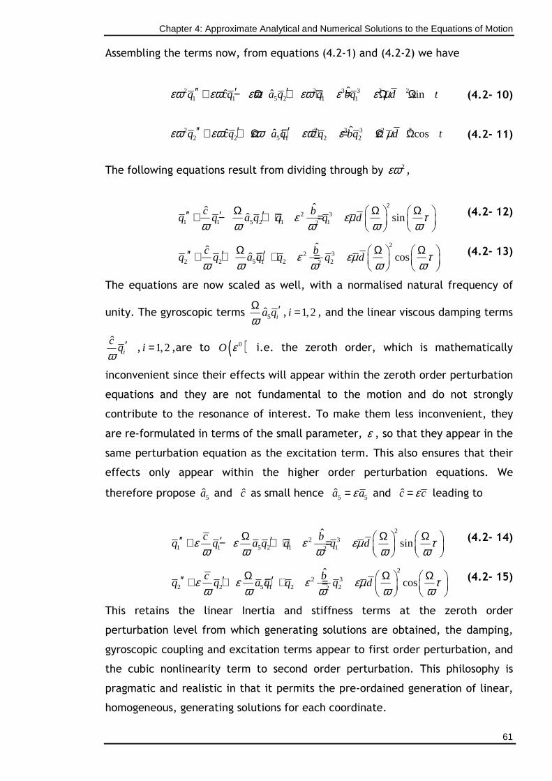
Chapter 4: Approximate Analytical and Numerical Solutions to the Equations of Motion
61
Assembling the terms now, from equations (4.2-1) and (4.2-2) we have
2 2 3 3 2 21 1 5 2 1 1
ˆˆ ˆ sinq cq a q q bq d tεω εω εω εω ε ε µ′′ ′ ′+ − Ω + + = Ω Ω (4.2- 10)
2 2 3 3 2 22 2 5 1 2 2
ˆˆ ˆ cosq cq a q q bq d tεω εω εω εω ε ε µ′′ ′ ′+ + Ω + + = Ω Ω (4.2- 11)
The following equations result from dividing through by 2εω ,
22 3
1 1 5 2 1 12
ˆˆˆ sin
c bq q a q q q dε εµ τ
ω ω ω ω ωΩ Ω Ω ′′ ′ ′+ − + + =
(4.2- 12)
22 3
2 2 5 1 2 22
ˆˆˆ cos
c bq q a q q q dε εµ τ
ω ω ω ω ωΩ Ω Ω ′′ ′ ′+ + + + =
(4.2- 13)
The equations are now scaled as well, with a normalised natural frequency of
unity. The gyroscopic terms 5ˆ ia qωΩ ′ , 1,2i = , and the linear viscous damping terms
ˆi
cq
ω′ , 1,2i = ,are to ( )0O ε i.e. the zeroth order, which is mathematically
inconvenient since their effects will appear within the zeroth order perturbation
equations and they are not fundamental to the motion and do not strongly
contribute to the resonance of interest. To make them less inconvenient, they
are re-formulated in terms of the small parameter, ε , so that they appear in the
same perturbation equation as the excitation term. This also ensures that their
effects only appear within the higher order perturbation equations. We
therefore propose 5a and c as small hence 5 5a aε= and c cε= leading to
22 3
1 1 5 2 1 12
ˆsin
c bq q a q q q dε ε ε εµ τ
ω ω ω ω ωΩ Ω Ω ′′ ′ ′+ − + + =
(4.2- 14)
22 3
2 2 5 1 2 22
ˆcos
c bq q a q q q dε ε ε εµ τ
ω ω ω ω ωΩ Ω Ω ′′ ′ ′+ + + + =
(4.2- 15)
This retains the linear Inertia and stiffness terms at the zeroth order
perturbation level from which generating solutions are obtained, the damping,
gyroscopic coupling and excitation terms appear to first order perturbation, and
the cubic nonlinearity term to second order perturbation. This philosophy is
pragmatic and realistic in that it permits the pre-ordained generation of linear,
homogeneous, generating solutions for each coordinate.
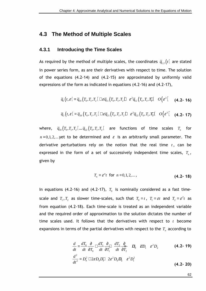
Chapter 4: Approximate Analytical and Numerical Solutions to the Equations of Motion
62
4.3 The Method of Multiple Scales
4.3.1 Introducing the Time Scales
As required by the method of multiple scales, the coordinates ( )1,2q t are stated
in power series form, as are their derivatives with respect to time. The solution
of the equations (4.2-14) and (4.2-15) are approximated by uniformly valid
expressions of the form as indicated in equations (4.2-16) and (4.2-17),
( ) ( ) ( ) ( ) ( )2 31 10 0 1 2 11 0 1 2 12 0 1 2, , , , , , ,q t q T T T q T T T q T T T Oε ε ε ε= + + + (4.2- 16)
( ) ( ) ( ) ( ) ( )2 32 20 0 1 2 21 0 1 2 22 0 1 2, , , , , , ,q t q T T T q T T T q T T T Oε ε ε ε= + + + (4.2- 17)
where, ( )10 0 1 2, ,q T T T … ( )22 0 1 2, ,q T T T are functions of time scales nT for
0,1,2,...n = yet to be determined and ε is an arbitrarily small parameter. The
derivative perturbations rely on the notion that the real time t , can be
expressed in the form of a set of successively independent time scales, nT ,
given by
nnT tε= for 0,1,2,...n = , (4.2- 18)
In equations (4.2-16) and (4.2-17), 0T is nominally considered as a fast time-
scale and 1T , 2T as slower time-scales, such that 0T t= , 1T tε= and 22T tε= as
from equation (4.2-18). Each time-scale is treated as an independent variable
and the required order of approximation to the solution dictates the number of
time scales used. It follows that the derivatives with respect to t become
expansions in terms of the partial derivatives with respect to the nT according to
20 1 20 1 2
0 1 2
22 2 2 20 0 1 0 2 12
2 2
dT dT dTdD D D
dt dt T dt T dt T
dD D D D D D
dt
ε ε
ε ε ε
∂ ∂ ∂= + + = + +∂ ∂ ∂
= + + +
(4.2- 19)
(4.2- 20)
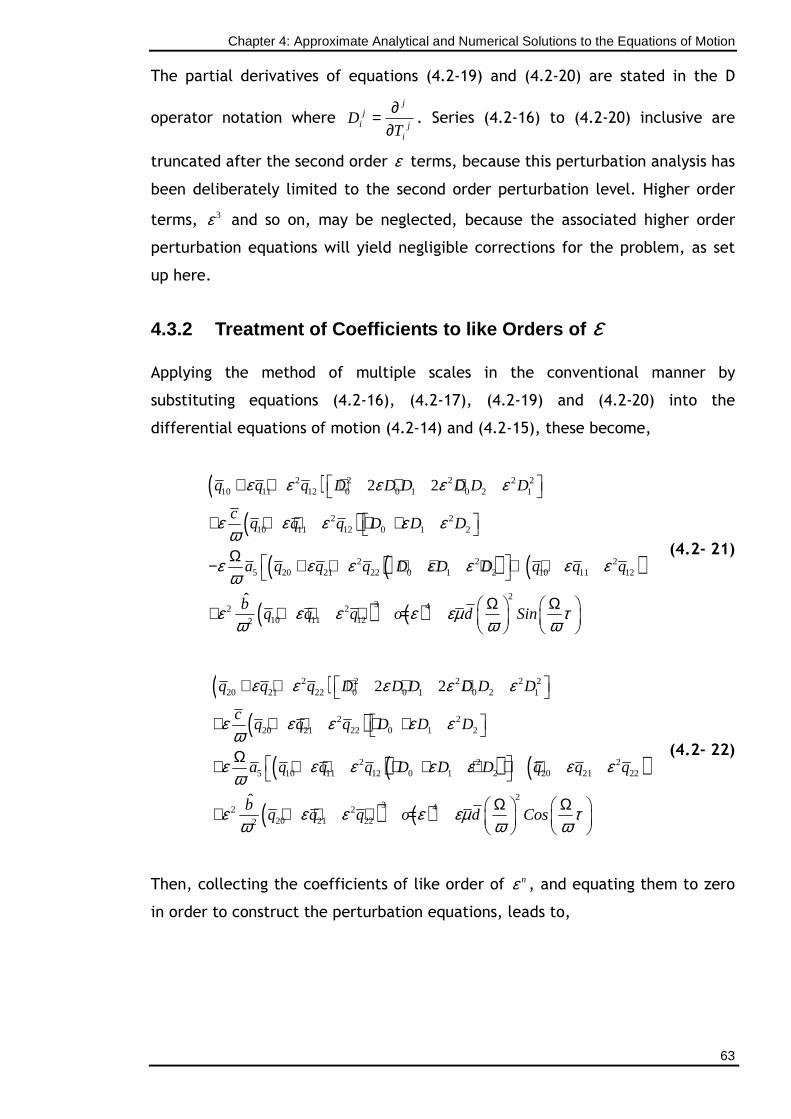
Chapter 4: Approximate Analytical and Numerical Solutions to the Equations of Motion
63
The partial derivatives of equations (4.2-19) and (4.2-20) are stated in the D
operator notation where j
i
jj
iT
D∂∂= . Series (4.2-16) to (4.2-20) inclusive are
truncated after the second order ε terms, because this perturbation analysis has
been deliberately limited to the second order perturbation level. Higher order
terms, 3ε and so on, may be neglected, because the associated higher order
perturbation equations will yield negligible corrections for the problem, as set
up here.
4.3.2 Treatment of Coefficients to like Orders of ε
Applying the method of multiple scales in the conventional manner by
substituting equations (4.2-16), (4.2-17), (4.2-19) and (4.2-20) into the
differential equations of motion (4.2-14) and (4.2-15), these become,
( )( )
( ) ( ) ( )
( ) ( )
2 2 2 2 210 11 12 0 0 1 0 2 1
2 210 11 12 0 1 2
2 2 25 20 21 22 0 1 2 10 11 12
23 42 2
10 11 122
2 2
ˆ
q q q D D D D D D
cq q q D D D
a q q q D D D q q q
bq q q o d Sin
ε ε ε ε ε
ε ε ε ε εω
ε ε ε ε ε ε εω
ε ε ε ε εµ τω ω ω
+ + + + +
+ + + + +
Ω − + + + + + + +
Ω Ω + + + + =
(4.2- 21)
( )( )
( ) ( ) ( )
( ) ( )
2 2 2 2 220 21 22 0 0 1 0 2 1
2 220 21 22 0 1 2
2 2 25 10 11 12 0 1 2 20 21 22
23 42 2
20 21 222
2 2
ˆ
q q q D D D D D D
cq q q D D D
a q q q D D D q q q
bq q q o d Cos
ε ε ε ε ε
ε ε ε ε εω
ε ε ε ε ε ε εω
ε ε ε ε εµ τω ω ω
+ + + + +
+ + + + +
Ω + + + + + + + +
Ω Ω + + + + =
(4.2- 22)
Then, collecting the coefficients of like order of nε , and equating them to zero
in order to construct the perturbation equations, leads to,
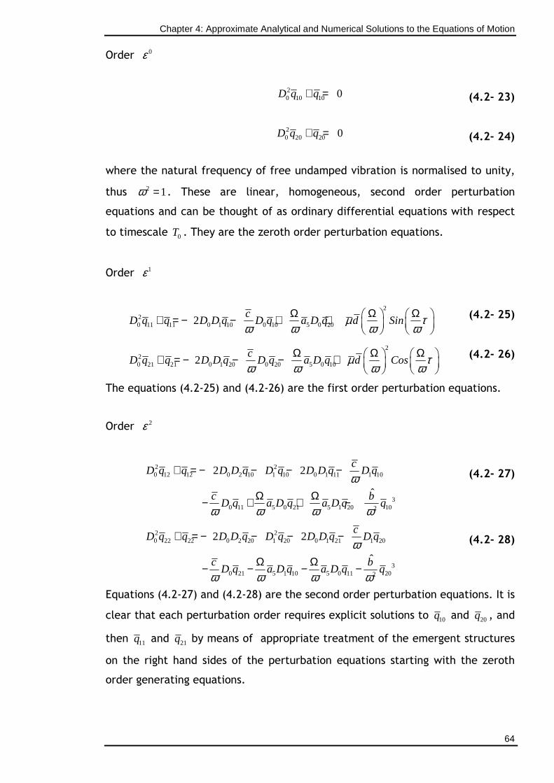
Chapter 4: Approximate Analytical and Numerical Solutions to the Equations of Motion
64
Order 0ε
20 10 10 0D q q+ = (4.2- 23)
20 20 20 0D q q+ = (4.2- 24)
where the natural frequency of free undamped vibration is normalised to unity,
thus 2 1ω = . These are linear, homogeneous, second order perturbation
equations and can be thought of as ordinary differential equations with respect
to timescale 0T . They are the zeroth order perturbation equations.
Order 1ε
220 11 11 0 1 10 0 10 5 0 202
cD q q D D q D q a D q d Sinµ τ
ω ω ω ωΩ Ω Ω + = − − + +
(4.2- 25)
220 21 21 0 1 20 0 20 5 0 102
cD q q D D q D q a D q d Cosµ τ
ω ω ω ωΩ Ω Ω + = − − − +
(4.2- 26)
The equations (4.2-25) and (4.2-26) are the first order perturbation equations.
Order 2ε
2 20 12 12 0 2 10 1 10 0 1 11 1 10
30 11 5 0 21 5 1 20 102
2 2
ˆ
cD q q D D q D q D D q D q
c bD q a D q a D q q
ω
ω ω ω ω
+ = − − − −
Ω Ω− + + −
(4.2- 27)
2 20 22 22 0 2 20 1 20 0 1 21 1 20
30 21 5 1 10 5 0 11 202
2 2
ˆ
cD q q D D q D q D D q D q
c bD q a D q a D q q
ω
ω ω ω ω
+ = − − − −
Ω Ω− − − −
(4.2- 28)
Equations (4.2-27) and (4.2-28) are the second order perturbation equations. It is
clear that each perturbation order requires explicit solutions to 10q and 20q , and
then 11q and 21q by means of appropriate treatment of the emergent structures
on the right hand sides of the perturbation equations starting with the zeroth
order generating equations.
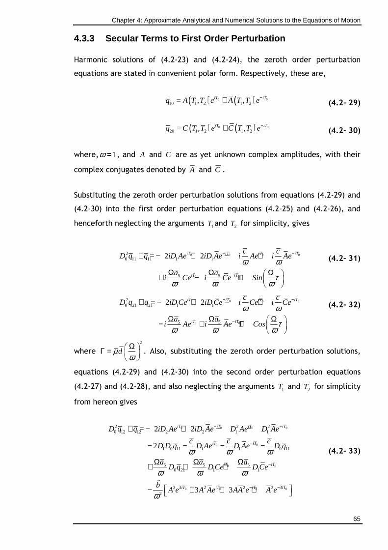
Chapter 4: Approximate Analytical and Numerical Solutions to the Equations of Motion
65
4.3.3 Secular Terms to First Order Perturbation
Harmonic solutions of (4.2-23) and (4.2-24), the zeroth order perturbation
equations are stated in convenient polar form. Respectively, these are,
( ) ( )0 010 1 2 1 2, ,iT iTq A T T e A T T e−= + (4.2- 29)
( ) ( )0 020 1 2 1 2, ,iT iTq C T T e C T T e−= + (4.2- 30)
where, 1ω = , and A and C are as yet unknown complex amplitudes, with their
complex conjugates denoted by A and C .
Substituting the zeroth order perturbation solutions from equations (4.2-29) and
(4.2-30) into the first order perturbation equations (4.2-25) and (4.2-26), and
henceforth neglecting the arguments 1T and 2T for simplicity, gives
0 0 0 0
0 0
20 11 11 1 1
5 5
2 2iT iT iT iT
iT iT
c cD q q iD Ae iD Ae i Ae i Ae
a ai Ce i Ce Sin
ω ω
τω ω ω
− −
−
+ = − + − +
Ω Ω Ω + − + Γ
(4.2- 31)
0 0 0 0
0 0
20 21 21 1 1
5 5
2 2iT iT iT iT
iT iT
c cD q q iD Ce iD Ce i Ce i Ce
a ai Ae i Ae Cos
ω ω
τω ω ω
− −
−
+ = − + − +
Ω Ω Ω − + + Γ
(4.2- 32)
where 2
dµωΩ Γ =
. Also, substituting the zeroth order perturbation solutions,
equations (4.2-29) and (4.2-30) into the second order perturbation equations
(4.2-27) and (4.2-28), and also neglecting the arguments 1T and 2T for simplicity
from hereon gives
0 0 0 0
0 0
0 0
0 0 0 0
2 2 20 12 12 2 2 1 1
1 0 11 1 1 0 11
5 5 50 21 1 1
3 33 2 2 32
2 2
2
ˆ3 3
iT iT iT iT
iT iT
iT iT
iT iT iT iT
D q q iD Ae iD Ae D Ae D Ae
c c cD D q D Ae D Ae D q
a a aD q D Ce D Ce
bA e A Ae AA e A e
ω ω ω
ω ω ω
ω
− −
−
−
− −
+ = − + − −
− − − −
Ω Ω Ω+ + +
− + + +
(4.2- 33)
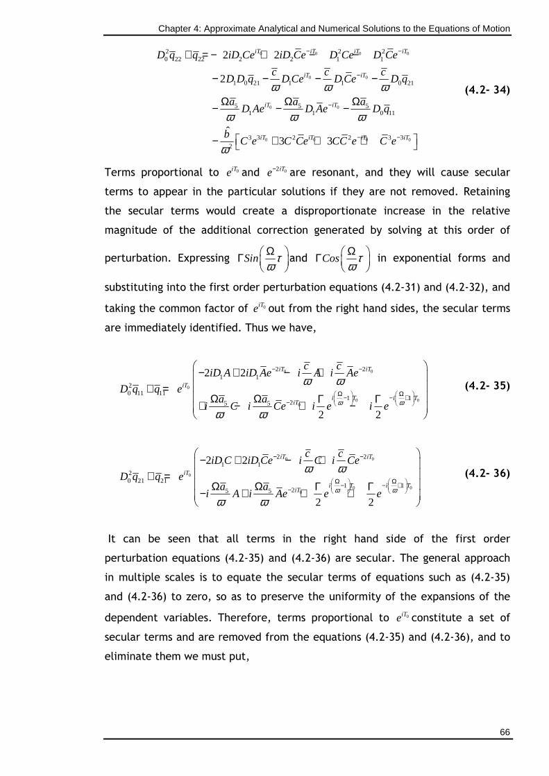
Chapter 4: Approximate Analytical and Numerical Solutions to the Equations of Motion
66
0 0 0 0
0 0
0 0
0 0 0 0
2 2 20 22 22 2 2 1 1
1 0 21 1 1 0 21
5 5 51 1 0 11
3 33 2 2 32
2 2
2
ˆ3 3
iT iT iT iT
iT iT
iT iT
iT iT iT iT
D q q iD Ce iD Ce D Ce D Ce
c c cD D q D Ce D Ce D q
a a aD Ae D Ae D q
bC e C Ce CC e C e
ω ω ω
ω ω ω
ω
− −
−
−
− −
+ = − + − −
− − − −
Ω Ω Ω− − −
− + + +
(4.2- 34)
Terms proportional to 0iTe and 02iTe− are resonant, and they will cause secular
terms to appear in the particular solutions if they are not removed. Retaining
the secular terms would create a disproportionate increase in the relative
magnitude of the additional correction generated by solving at this order of
perturbation. Expressing Sin τωΩ Γ
and Cos τωΩ Γ
in exponential forms and
substituting into the first order perturbation equations (4.2-31) and (4.2-32), and
taking the common factor of 0iTe out from the right hand sides, the secular terms
are immediately identified. Thus we have,
0 0
0
0 00
2 21 1
20 11 11
1 125 5
2 2
2 2
iT iT
iT
i T i TiT
c ciD A iD Ae i A i Ae
D q q ea a
i C i Ce i e i eω ω
ω ω
ω ω
− −
Ω Ω − − + −
− + − + + = Ω Ω Γ Γ+ − + −
(4.2- 35)
0 0
0
0 00
2 21 1
20 21 21
1 125 5
2 2
2 2
iT iT
iT
i T i TiT
c ciD C iD Ce i C i Ce
D q q ea a
i A i Ae e eω ω
ω ω
ω ω
− −
Ω Ω − − + −
− + − + + = Ω Ω Γ Γ− + + +
(4.2- 36)
It can be seen that all terms in the right hand side of the first order
perturbation equations (4.2-35) and (4.2-36) are secular. The general approach
in multiple scales is to equate the secular terms of equations such as (4.2-35)
and (4.2-36) to zero, so as to preserve the uniformity of the expansions of the
dependent variables. Therefore, terms proportional to 0iTe constitute a set of
secular terms and are removed from the equations (4.2-35) and (4.2-36), and to
eliminate them we must put,
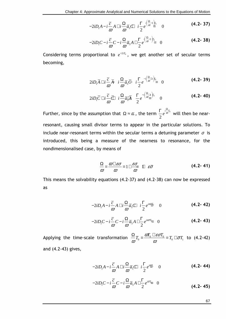
Chapter 4: Approximate Analytical and Numerical Solutions to the Equations of Motion
67
01
1 52 02
i TciD A i A i a C i e ω
ω ω
Ω − Ω Γ− − + + = (4.2- 37)
01
1 52 02
i TciD C i C i a A e ω
ω ω
Ω − Ω Γ− − − + = (4.2- 38)
Considering terms proportional to 02iTe− , we get another set of secular terms
becoming,
01
1 52 02
i TciD A i A i a C i e ω
ω ω
Ω − + Ω Γ+ − − = (4.2- 39)
01
1 52 02
i TciD C i C i a A e ω
ω ω
Ω − + Ω Γ+ + + = (4.2- 40)
Further, since by the assumption that ω≈Ω , the term 0
2
i Te ω
ΩΓ will then be near-
resonant, causing small divisor terms to appear in the particular solutions. To
include near-resonant terms within the secular terms a detuning parameter σ is
introduced, this being a measure of the nearness to resonance, for the
nondimensionalised case, by means of
1 1
ω εσ εσ εσω ω ωΩ += = + = + (4.2- 41)
This means the solvability equations (4.2-37) and (4.2-38) can now be expressed
as
0
1 52 02
i TciD A i A i a C i e εσ
ω ωΩ Γ− − + + = (4.2- 42)
0
1 52 02
i TciD C i C i a A e εσ
ω ωΩ Γ− − − + = (4.2- 43)
Applying the time-scale transformation 0 00 0 1
T TT T T
ω εσ σω ω
+Ω = = + to (4.2-42)
and (4.2-43) gives,
1
1 52 02
i TciD A i A i a C i e σ
ω ωΩ Γ− − + + = (4.2- 44)
1
1 52 02
i TciD C i C i a A e σ
ω ωΩ Γ− − − + =
(4.2- 45)
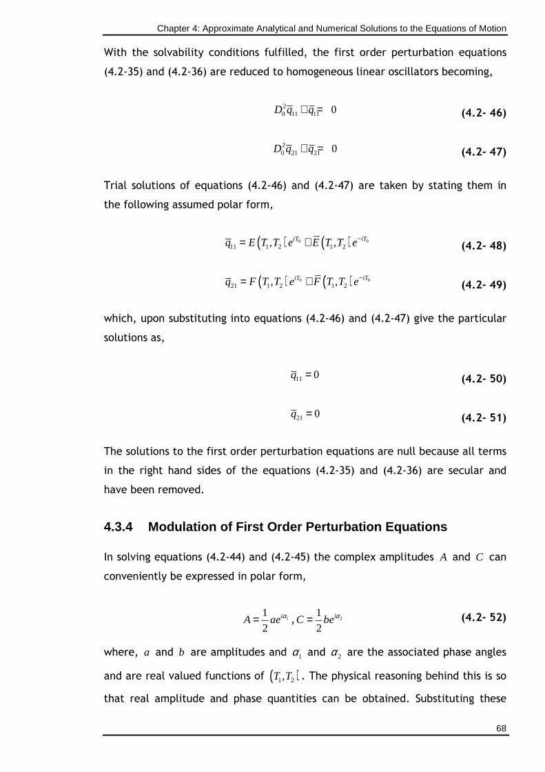
Chapter 4: Approximate Analytical and Numerical Solutions to the Equations of Motion
68
With the solvability conditions fulfilled, the first order perturbation equations
(4.2-35) and (4.2-36) are reduced to homogeneous linear oscillators becoming,
20 11 11 0D q q+ = (4.2- 46)
2
0 21 21 0D q q+ = (4.2- 47)
Trial solutions of equations (4.2-46) and (4.2-47) are taken by stating them in
the following assumed polar form,
( ) ( )0 011 1 2 1 2, , −= +iT iTq E T T e E T T e (4.2- 48)
( ) ( )0 0
21 1 2 1 2, , −= +iT iTq F T T e F T T e (4.2- 49)
which, upon substituting into equations (4.2-46) and (4.2-47) give the particular
solutions as,
11 0q = (4.2- 50)
21 0q = (4.2- 51)
The solutions to the first order perturbation equations are null because all terms
in the right hand sides of the equations (4.2-35) and (4.2-36) are secular and
have been removed.
4.3.4 Modulation of First Order Perturbation Equati ons
In solving equations (4.2-44) and (4.2-45) the complex amplitudes A and C can
conveniently be expressed in polar form,
1
1
2iA ae α= , 2
1
2iC be α= (4.2- 52)
where, a and b are amplitudes and 1α and 2α are the associated phase angles
and are real valued functions of ( )1 2,T T . The physical reasoning behind this is so
that real amplitude and phase quantities can be obtained. Substituting these
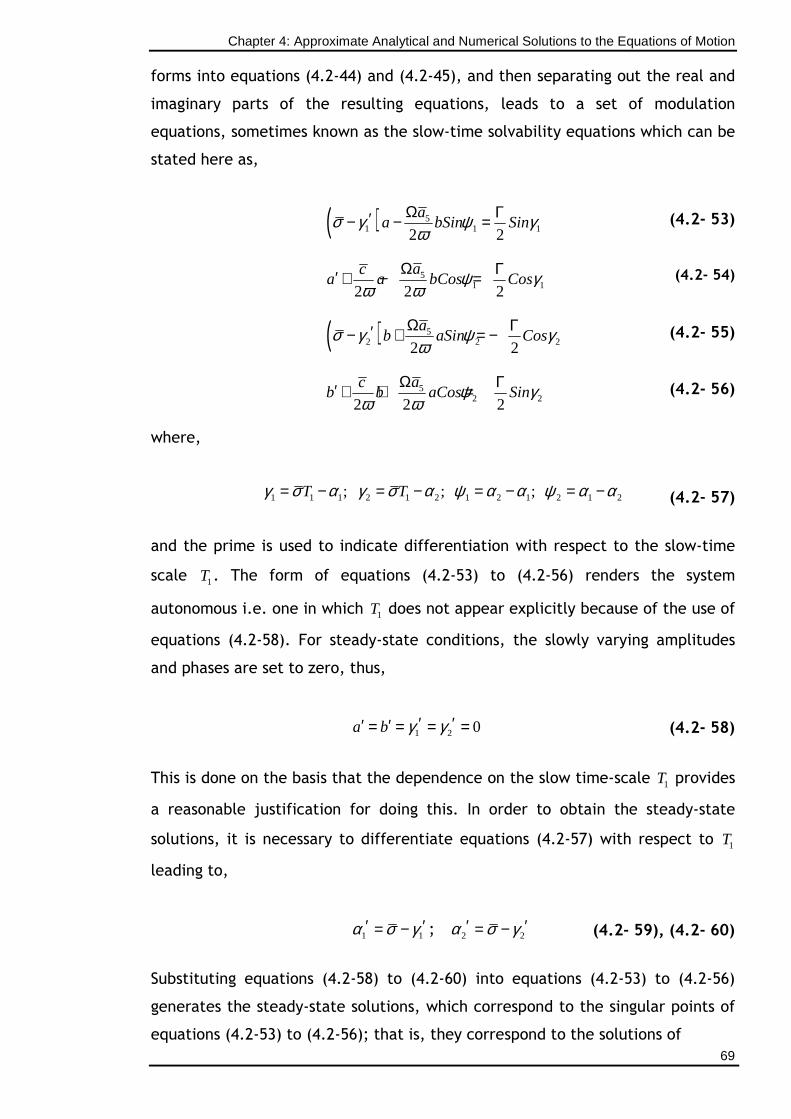
Chapter 4: Approximate Analytical and Numerical Solutions to the Equations of Motion
69
forms into equations (4.2-44) and (4.2-45), and then separating out the real and
imaginary parts of the resulting equations, leads to a set of modulation
equations, sometimes known as the slow-time solvability equations which can be
stated here as,
( ) 51 1 12 2
σ γ ψ γω
Ω Γ′− − =aa bSin Sin (4.2- 53)
51 12 2 2
ψ γω ω
Ω Γ′ + − =aca a bCos Cos (4.2- 54)
( ) 52 2 22 2
σ γ ψ γω
Ω Γ′− + = −ab aSin Cos (4.2- 55)
52 22 2 2
ψ γω ω
Ω Γ′ + + =acb b aCos Sin (4.2- 56)
where,
1 1 1 2 1 2 1 2 1 2 1 2; ; ;γ σ α γ σ α ψ α α ψ α α= − = − = − = −T T (4.2- 57)
and the prime is used to indicate differentiation with respect to the slow-time
scale 1T . The form of equations (4.2-53) to (4.2-56) renders the system
autonomous i.e. one in which 1T does not appear explicitly because of the use of
equations (4.2-58). For steady-state conditions, the slowly varying amplitudes
and phases are set to zero, thus,
1 2 0a b γ γ′ ′′ ′= = = = (4.2- 58)
This is done on the basis that the dependence on the slow time-scale 1T provides
a reasonable justification for doing this. In order to obtain the steady-state
solutions, it is necessary to differentiate equations (4.2-57) with respect to 1T
leading to,
1 1α σ γ′ ′= − ; 2 2α σ γ′ ′= − (4.2- 59), (4.2- 60)
Substituting equations (4.2-58) to (4.2-60) into equations (4.2-53) to (4.2-56)
generates the steady-state solutions, which correspond to the singular points of
equations (4.2-53) to (4.2-56); that is, they correspond to the solutions of
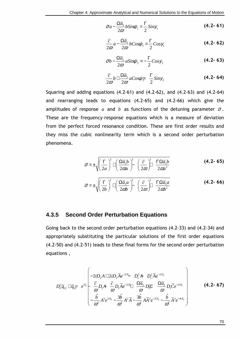
Chapter 4: Approximate Analytical and Numerical Solutions to the Equations of Motion
70
51 12 2
aa bSin Sinσ ψ γ
ωΩ Γ− = (4.2- 61)
51 12 2 2
aca bCos Cosψ γ
ω ωΩ Γ− = (4.2- 62)
52 22 2
ab aSin Cosσ ψ γ
ωΩ Γ− = − (4.2- 63)
52 22 2 2
acb aCos Sinψ γ
ω ωΩ Γ+ = (4.2- 64)
Squaring and adding equations (4.2-61) and (4.2-62), and (4.2-63) and (4.2-64)
and rearranging leads to equations (4.2-65) and (4.2-66) which give the
amplitudes of response a and b as functions of the detuning parameter σ .
These are the frequency–response equations which is a measure of deviation
from the perfect forced resonance condition. These are first order results and
they miss the cubic nonlinearity term which is a second order perturbation
phenomena.
22 2
5 522 2 2 2
a b a bc
a a aσ
ω ω ωΩ ΓΩΓ = ± + − +
(4.2- 65)
22 2
5 522 2 2 2
a a a ac
b b bσ
ω ω ωΩ ΓΩΓ = ± + − +
(4.2- 66)
4.3.5 Second Order Perturbation Equations
Going back to the second order perturbation equations (4.2-33) and (4.2-34) and
appropriately substituting the particular solutions of the first order equations
(4.2-50) and (4.2-51) leads to these final forms for the second order perturbation
equations ,
0 0
0 0 0
0 0 0
2 22 22 2 1 1
2 22 5 50 12 12 1 1 1 1
2 2 43 2 2 32 2 2 2
2 2
ˆ ˆ ˆ ˆ3 3
iT iT
iT iT iT
iT iT iT
iD A iD Ae D A D Ae
a ac cD q q e D A D Ae D C D Ce
b b b bA e A A AA e A e
ω ω ω ω
ω ω ω ω
− −
− −
− −
− + − −
Ω Ω + = − − + + − − − −
(4.2- 67)
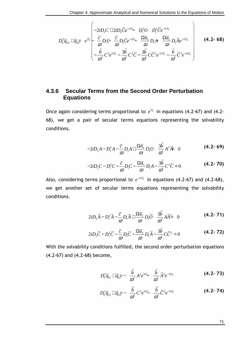
Chapter 4: Approximate Analytical and Numerical Solutions to the Equations of Motion
71
0 0
0 0 0
0 0 0
2 22 22 2 1 1
2 22 5 50 22 22 1 1 1 1
2 2 43 2 2 32 2 2 2
2 2
ˆ ˆ ˆ ˆ3 3
iT iT
iT iT iT
iT iT iT
iD C iD Ce D C D Ce
a ac cD q q e D C D Ce D A D Ae
b b b bC e C C CC e C e
ω ω ω ω
ω ω ω ω
− −
− −
− −
− + − −
Ω Ω + = − − − − − − − −
(4.2- 68)
4.3.6 Secular Terms from the Second Order Perturbat ion Equations
Once again considering terms proportional to 0iTe in equations (4.2-67) and (4.2-
68), we get a pair of secular terms equations representing the solvability
conditions.
2 25
2 1 1 1 2
ˆ32 0
ac biD A D A D A D C A A
ω ω ωΩ− − − + − = (4.2- 69)
2 25
2 1 1 1 2
ˆ32 0
ac biD C D C D C D A C C
ω ω ωΩ− − − − − = (4.2- 70)
Also, considering terms proportional to 02iTe− in equations (4.2-67) and (4.2-68),
we get another set of secular terms equations representing the solvability
conditions.
2 25
2 1 1 1 2
ˆ32 0
ac biD A D A D A D C AA
ω ω ωΩ− − + − = (4.2- 71)
2 25
2 1 1 1 2
ˆ32 0
ac biD C D C D C D A CC
ω ω ωΩ− − − − = (4.2- 72)
With the solvability conditions fulfilled, the second order perturbation equations
(4.2-67) and (4.2-68) become,
0 03 32 3 3
0 12 12 2 2
ˆ ˆiT iTb b
D q q A e A eω ω
−+ = − − (4.2- 73)
0 03 32 3 3
0 22 22 2 2
ˆ ˆiT iTb b
D q q C e C eω ω
−+ = − − (4.2- 74)
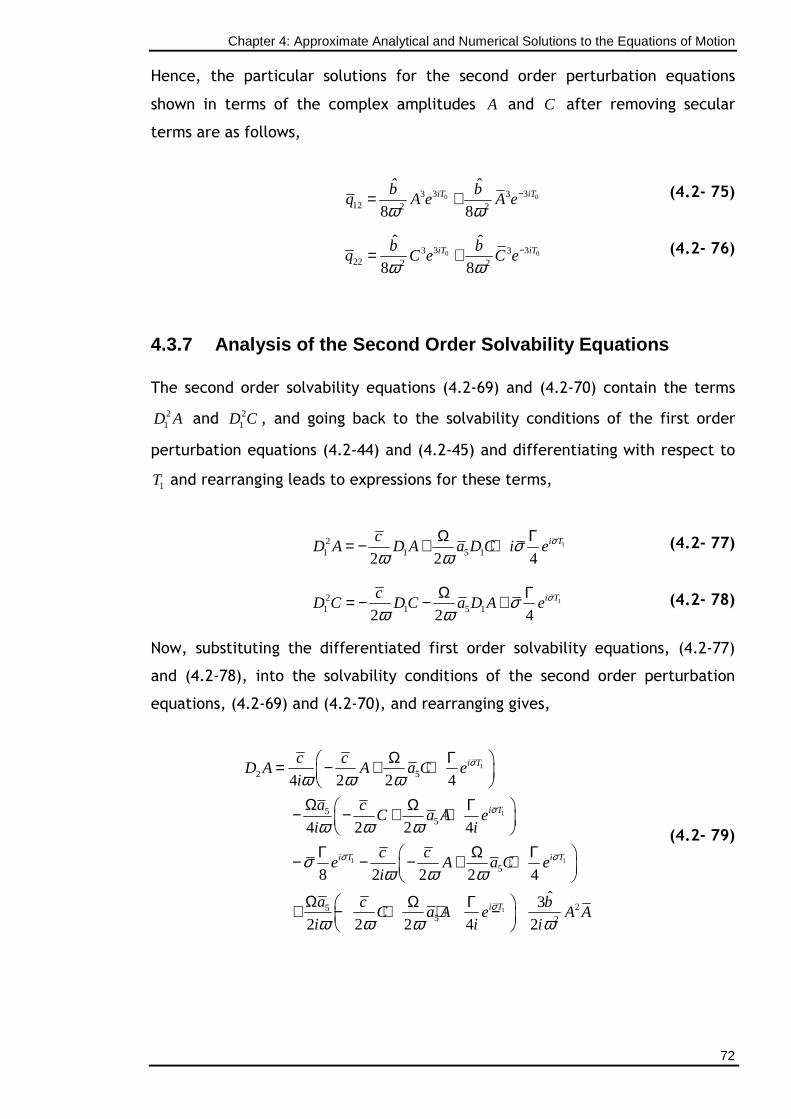
Chapter 4: Approximate Analytical and Numerical Solutions to the Equations of Motion
72
Hence, the particular solutions for the second order perturbation equations
shown in terms of the complex amplitudes A and C after removing secular
terms are as follows,
0 03 33 3
12 2 2
ˆ ˆ
8 8iT iTb b
q A e A eω ω
−= + (4.2- 75)
0 03 33 3
22 2 2
ˆ ˆ
8 8iT iTb b
q C e C eω ω
−= + (4.2- 76)
4.3.7 Analysis of the Second Order Solvability Equa tions
The second order solvability equations (4.2-69) and (4.2-70) contain the terms
21D A and 2
1D C , and going back to the solvability conditions of the first order
perturbation equations (4.2-44) and (4.2-45) and differentiating with respect to
1T and rearranging leads to expressions for these terms,
12
1 1 5 12 2 4i Tc
D A D A a D C i e σσω ω
Ω Γ= − + + (4.2- 77)
12
1 1 5 12 2 4i Tc
D C D C a D A e σσω ω
Ω Γ= − − + (4.2- 78)
Now, substituting the differentiated first order solvability equations, (4.2-77)
and (4.2-78), into the solvability conditions of the second order perturbation
equations, (4.2-69) and (4.2-70), and rearranging gives,
1
1
1 1
1
2 5
55
5
255 2
4 2 2 4
4 2 2 4
8 2 2 2 4
ˆ3
2 2 2 4 2
i T
i T
i T i T
i T
c cD A A a C e
i
a cC a A e
i i
c ce A a C e
i
a c bC a A e A A
i i i
σ
σ
σ σ
σ
ω ω ω
ω ω ω
σω ω ω
ω ω ω ω
Ω Γ = − + +
Ω Ω Γ − − + +
Γ Ω Γ − − − + +
Ω Ω Γ + − + + −
(4.2- 79)
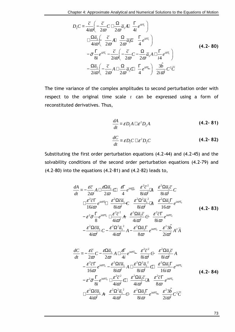
Chapter 4: Approximate Analytical and Numerical Solutions to the Equations of Motion
73
1
1
1 1
1
2 5
55
5
255 2
4 2 2 4
4 2 2 4
8 2 2 2 4
ˆ3
2 2 2 4 2
i T
i T
i T i T
i T
c cD C C a A e
i i
a cA a C e
i
c ce C a A e
i i i
a c bA a C e C C
i i
σ
σ
σ σ
σ
ω ω ω
ω ω ω
σω ω ω
ω ω ω ω
Ω Γ = − + +
Ω Ω Γ + − + +
Γ Ω Γ − − − − +
Ω Ω Γ − − + + −
(4.2- 80)
The time variance of the complex amplitudes to second perturbation order with
respect to the original time scale t can be expressed using a form of
reconstituted derivatives. Thus,
21 2
dAD A D A
dtε ε= + (4.2- 81)
21 2
dCD C D C
dtε ε= + (4.2- 82)
Substituting the first order perturbation equations (4.2-44) and (4.2-45) and the
solvability conditions of the second order perturbation equations (4.2-79) and
(4.2-80) into the equations (4.2-81) and (4.2-82) leads to,
0
0 0
0 0
0
22 25 5
2 2
2 2 2 2 225 5 5
2 2
22 2 22 5
2 2
2 2 2 2 2 25 5 5
2 2
2 2 4 8 8
16 8 8 16
8 4 4 8ˆ3
4 4 8
i T
i T i T
i T i T
i T
a a cdA c cA C e A C
dt i i
ca a ace C A e
i i i
a cc ce A C e
i i i
ca a aC A e
i i
εσ
εσ εσ
εσ εσ
εσ
ε εε ε εω ω ω ω
ε ε εεω ω ω ω
εε εε σω ω ω
ε ε ε εω ω ω
Ω ΩΓ= − + + − +
Ω Ω Ω ΓΓ+ + − +
ΩΓ Γ− + − −
Ω Ω Ω Γ− − − − 222
bA A
iω
(4.2- 83)
0
0 0
0 0
0
22 25 5
2 2
2 2 2 2 225 5 5
2 2
22 2 22 5
2 2
2 2 2 2 2 25 5 5
2 2
2 2 4 8 8
16 8 8 16
8 4 4 8
4 4 8
i T
i T i T
i T i T
i T
a a cdC c cC A e C A
dt i i i
ca a ace A C e
i i i
a cc ce C A e
i i i
ca a aA C e
i i i
εσ
εσ εσ
εσ εσ
εσ
ε εε ε εω ω ω ω
ε ε εεω ω ω ω
εε εε σω ω ω
ε ε ε εω ω ω
Ω ΩΓ= − − + − −
Ω Ω Ω ΓΓ− − + +
ΩΓ Γ− + + +
Ω Ω Ω Γ+ − − − 22
ˆ3
2
bC C
iω
(4.2- 84)
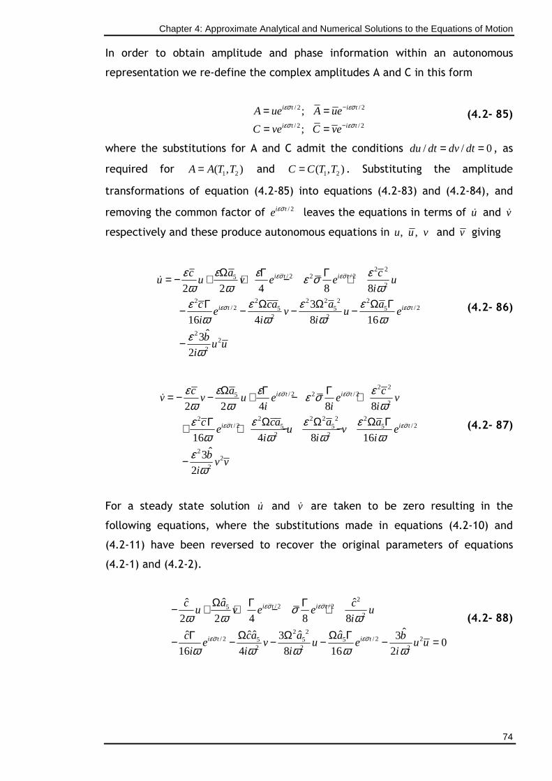
Chapter 4: Approximate Analytical and Numerical Solutions to the Equations of Motion
74
In order to obtain amplitude and phase information within an autonomous
representation we re-define the complex amplitudes A and C in this form
/ 2 / 2
/ 2 / 2
;
;
εσ εσ
εσ εσ
−
−
= == =
i t i t
i t i t
A ue A ue
C ve C ve (4.2- 85)
where the substitutions for A and C admit the conditions / / 0du dt dv dt= = , as
required for 1 2( , )A A T T= and 1 2( , )C C T T= . Substituting the amplitude
transformations of equation (4.2-85) into equations (4.2-83) and (4.2-84), and
removing the common factor of / 2εσi te leaves the equations in terms of uɺ and vɺ
respectively and these produce autonomous equations in , ,u u v and v giving
2 2/ 2 2 / 25
2
2 2 2 2 22/ 2 / 25 5 5
2 2
22
2
2 2 4 8 8
3
16 4 8 16ˆ3
2
εσ εσ
εσ εσ
εε ε εε σω ω ω
ε ε εεω ω ω ω
εω
Ω Γ Γ= − + + − +
Ω Ω Ω ΓΓ− − − −
−
ɺi t i t
i t i t
ac cu u v e e u
i
ca a ace v u e
i i i
bu u
i
(4.2- 86)
2 2/ 2 2 / 25
2
2 2 2 2 22/ 2 / 25 5 5
2 2
22
2
2 2 4 8 8
16 4 8 16ˆ3
2
εσ εσ
εσ εσ
εε ε εε σω ω ω
ε ε εεω ω ω ω
εω
Ω Γ Γ= − − + − +
Ω Ω Ω ΓΓ+ + − −
−
ɺi t i t
i t i t
ac cv v u e e v
i i i
ca a ace u v e
i i i
bv v
i
(4.2- 87)
For a steady state solution uɺ and vɺ are taken to be zero resulting in the
following equations, where the substitutions made in equations (4.2-10) and
(4.2-11) have been reversed to recover the original parameters of equations
(4.2-1) and (4.2-2).
2/ 2 / 25
2
2 2/ 2 / 2 25 5 5
2 2 2
ˆˆ ˆ
2 2 4 8 8ˆˆ ˆ ˆ ˆˆ 3 3
016 4 8 16 2
i t i t
i t i t
ac cu v e e u
i
ca a ac be v u e u u
i i i i
εσ εσ
εσ εσ
σω ω ω
ω ω ω ω ω
Ω Γ Γ− + + − +
Ω Ω Ω ΓΓ− − − − − =
(4.2- 88)
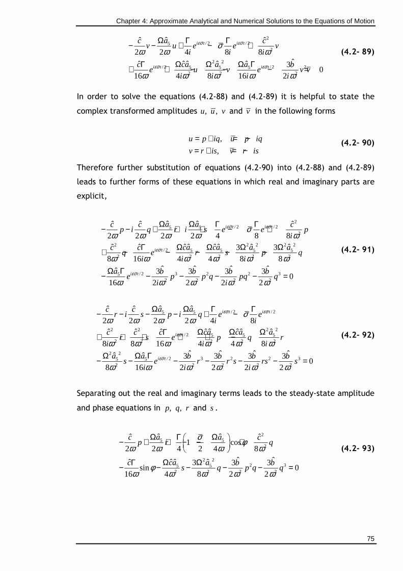
Chapter 4: Approximate Analytical and Numerical Solutions to the Equations of Motion
75
2/ 2 / 25
2
2 2/ 2 / 2 25 5 5
2 2 2
ˆˆ ˆ
2 2 4 8 8ˆˆ ˆ ˆ ˆˆ 3
016 4 8 16 2
i t i t
i t i t
ac cv u e e v
i i i
ca a ac be u v e v v
i i i i
εσ εσ
εσ εσ
σω ω ω
ω ω ω ω ω
Ω Γ Γ− − + − +
Ω Ω Ω ΓΓ+ + − − − =
(4.2- 89)
In order to solve the equations (4.2-88) and (4.2-89) it is helpful to state the
complex transformed amplitudes , ,u u v and v in the following forms
,
,
= + = −= + = −
u p iq u p iq
v r is v r is (4.2- 90)
Therefore further substitution of equations (4.2-90) into (4.2-88) and (4.2-89)
leads to further forms of these equations in which real and imaginary parts are
explicit,
2/ 2 / 25 5
2
2 2 2 22/ 2 5 5 5 5
2 2 2 2 2
/ 2 3 2 2 352 2 2 2
ˆ ˆˆ ˆ ˆ
2 2 2 2 4 8 8ˆ ˆ ˆ ˆ ˆ ˆˆ ˆ 3 3
8 16 4 4 8 8ˆ ˆ ˆ ˆˆ 3 3 3 3
016 2 2 2 2
i t i t
i t
i t
a ac c cp i q r i s e e p
i
ca ca a ac cq e r s p q
i i i
a b b b be p p q pq q
i i
εσ εσ
εσ
εσ
σω ω ω ω ω
ω ω ω ω ω ω
ω ω ω ω ω
Ω Ω Γ Γ− − + + + − +
Ω Ω Ω ΩΓ+ − − − − −
Ω Γ− − − − − =
(4.2- 91)
/ 2 / 25 5
2 22 2/ 2 5 5 5
2 2 2 2 2
2 2/ 2 3 2 2 35 5
2 2 2 2 2
ˆ ˆˆ ˆ
2 2 2 2 4 8ˆ ˆ ˆ ˆ ˆˆ ˆ ˆ
8 8 16 4 4 8ˆ ˆ ˆ ˆˆ ˆ 3 3 3 3
08 16 2 2 2 2
i t i t
i t
i t
a ac cr i s p i q e e
i i
ca ca ac c cr s e p q r
i i i
a a b b b bs e r r s rs s
i i i
εσ εσ
εσ
εσ
σω ω ω ω
ω ω ω ω ω ω
ω ω ω ω ω ω
Ω Ω Γ Γ− − − − + −
Ω Ω ΩΓ+ + + + + −
Ω Ω Γ− − − − − − =
(4.2- 92)
Separating out the real and imaginary terms leads to the steady-state amplitude
and phase equations in , ,p q r and s .
25 5
2
2 22 35 5
2 2 2 2
ˆ ˆˆ ˆ1 cos
2 2 4 2 4 8
ˆ ˆˆ ˆ ˆˆ 3 3 3sin 0
16 4 8 2 2
a ac cp r q
ca ac b bs q p q q
σ φω ω ω ω
φω ω ω ω ω
Ω ΩΓ − + + − − +
Ω ΩΓ− − − − − =
(4.2- 93)
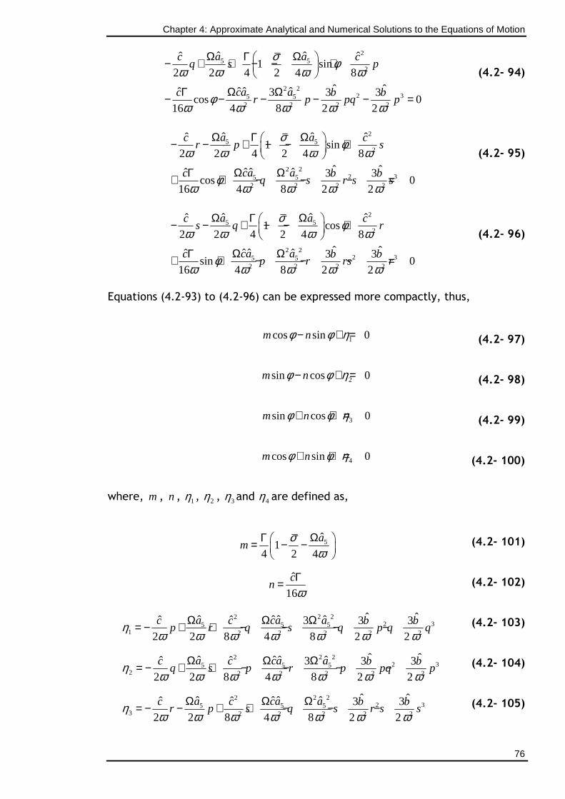
Chapter 4: Approximate Analytical and Numerical Solutions to the Equations of Motion
76
25 5
2
2 22 35 5
2 2 2 2
ˆ ˆˆ ˆ1 sin
2 2 4 2 4 8
ˆ ˆˆ ˆ ˆˆ 3 3 3cos 0
16 4 8 2 2
a ac cq s p
ca ac b br p pq p
σ φω ω ω ω
φω ω ω ω ω
Ω ΩΓ − + + − − +
Ω ΩΓ− − − − − =
(4.2- 94)
25 5
2
2 22 35 5
2 2 2 2
ˆ ˆˆ ˆ1 sin
2 2 4 2 4 8
ˆ ˆˆ ˆ ˆˆ 3 3cos 0
16 4 8 2 2
a ac cr p s
ca ac b bq s r s s
σ φω ω ω ω
φω ω ω ω ω
Ω ΩΓ − − + − − +
Ω ΩΓ+ + − − − =
(4.2- 95)
25 5
2
2 22 35 5
2 2 2 2
ˆ ˆˆ ˆ1 cos
2 2 4 2 4 8
ˆ ˆˆ ˆ ˆˆ 3 3sin 0
16 4 8 2 2
a ac cs q r
ca ac b bp r rs r
σ φω ω ω ω
φω ω ω ω ω
Ω ΩΓ − − + − − +
Ω ΩΓ+ + − − − =
(4.2- 96)
Equations (4.2-93) to (4.2-96) can be expressed more compactly, thus,
1cos sin 0m nφ φ η− + = (4.2- 97)
2sin cos 0m nφ φ η− + = (4.2- 98)
3sin cos 0m nφ φ η+ + = (4.2- 99)
4cos sin 0m nφ φ η+ + = (4.2- 100)
where, m , n , 1η , 2η , 3η and 4η are defined as,
5ˆ1
4 2 4
am
σω
ΩΓ = − −
(4.2- 101)
ˆ
16
cn
ωΓ= (4.2- 102)
2 222 35 5 5
1 2 2 2 2 2
ˆ ˆˆ ˆ ˆ ˆˆ ˆ 3 3 3
2 2 8 4 8 2 2
a ca ac c b bp r q s q p q qη
ω ω ω ω ω ω ωΩ Ω Ω= − + + − − − − (4.2- 103)
2 222 35 5 5
2 2 2 2 2 2
ˆ ˆˆ ˆ ˆ ˆˆ ˆ 3 3 3
2 2 8 4 8 2 2
a ca ac c b bq s p r p pq pη
ω ω ω ω ω ω ωΩ Ω Ω= − + + − − − − (4.2- 104)
2 222 35 5 5
3 2 2 2 2 2
ˆ ˆˆ ˆ ˆ ˆˆ ˆ 3 3
2 2 8 4 8 2 2
a ca ac c b br p s q s r s sη
ω ω ω ω ω ω ωΩ Ω Ω= − − + + − − − (4.2- 105)
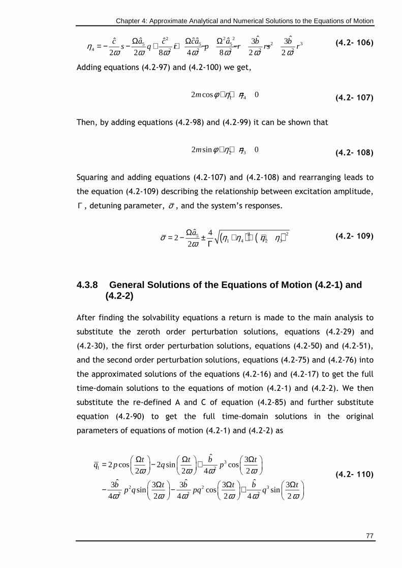
Chapter 4: Approximate Analytical and Numerical Solutions to the Equations of Motion
77
2 222 35 5 5
4 2 2 2 2 2
ˆ ˆˆ ˆ ˆ ˆˆ ˆ 3 3
2 2 8 4 8 2 2
a ca ac c b bs q r p r rs rη
ω ω ω ω ω ω ωΩ Ω Ω= − − + + − − − (4.2- 106)
Adding equations (4.2-97) and (4.2-100) we get,
1 42 cos 0m φ η η+ + = (4.2- 107)
Then, by adding equations (4.2-98) and (4.2-99) it can be shown that
2 32 sin 0m φ η η+ + = (4.2- 108)
Squaring and adding equations (4.2-107) and (4.2-108) and rearranging leads to
the equation (4.2-109) describing the relationship between excitation amplitude,
Γ , detuning parameter, σ , and the system’s responses.
( ) ( )2 251 4 2 3
ˆ 42
2
aσ η η η ηω
Ω= − ± + + +Γ
(4.2- 109)
4.3.8 General Solutions of the Equations of Motion (4.2-1) and (4.2-2)
After finding the solvability equations a return is made to the main analysis to
substitute the zeroth order perturbation solutions, equations (4.2-29) and
(4.2-30), the first order perturbation solutions, equations (4.2-50) and (4.2-51),
and the second order perturbation solutions, equations (4.2-75) and (4.2-76) into
the approximated solutions of the equations (4.2-16) and (4.2-17) to get the full
time-domain solutions to the equations of motion (4.2-1) and (4.2-2). We then
substitute the re-defined A and C of equation (4.2-85) and further substitute
equation (4.2-90) to get the full time-domain solutions in the original
parameters of equations of motion (4.2-1) and (4.2-2) as
3
1 2
2 2 32 2 2
ˆ 32 cos 2 sin cos
2 2 4 2
ˆ ˆ ˆ3 3 3 3 3sin cos sin
4 2 4 2 4 2
t t b tq p q p
b t b t b tp q pq q
ω ω ω ω
ω ω ω ω ω ω
Ω Ω Ω = − +
Ω Ω Ω − − +
(4.2- 110)
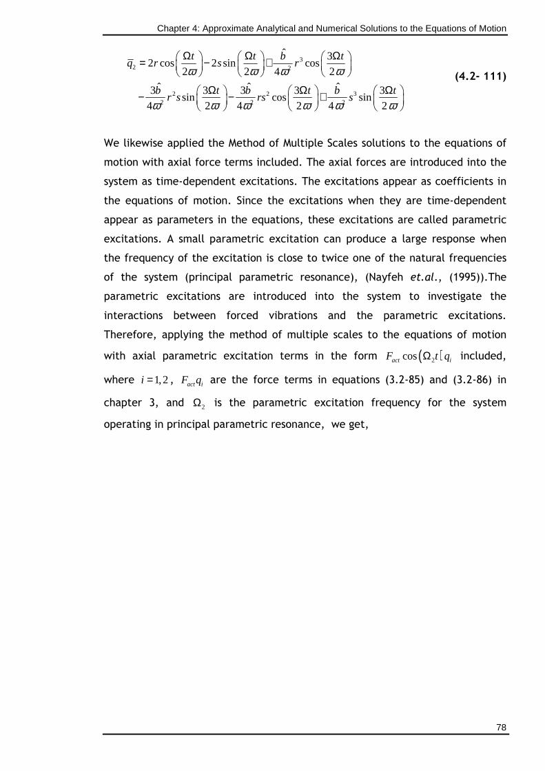
Chapter 4: Approximate Analytical and Numerical Solutions to the Equations of Motion
78
3
2 2
2 2 32 2 2
ˆ 32 cos 2 sin cos
2 2 4 2
ˆ ˆ ˆ3 3 3 3 3sin cos sin
4 2 4 2 4 2
t t b tq r s r
b t b t b tr s rs s
ω ω ω ω
ω ω ω ω ω ω
Ω Ω Ω = − +
Ω Ω Ω − − +
(4.2- 111)
We likewise applied the Method of Multiple Scales solutions to the equations of
motion with axial force terms included. The axial forces are introduced into the
system as time-dependent excitations. The excitations appear as coefficients in
the equations of motion. Since the excitations when they are time-dependent
appear as parameters in the equations, these excitations are called parametric
excitations. A small parametric excitation can produce a large response when
the frequency of the excitation is close to twice one of the natural frequencies
of the system (principal parametric resonance), (Nayfeh et.al., (1995)).The
parametric excitations are introduced into the system to investigate the
interactions between forced vibrations and the parametric excitations.
Therefore, applying the method of multiple scales to the equations of motion
with axial parametric excitation terms in the form ( )2cos Ωact iF t q included,
where 1,2i = , act iF q are the force terms in equations (3.2-85) and (3.2-86) in
chapter 3, and 2Ω is the parametric excitation frequency for the system
operating in principal parametric resonance, we get,
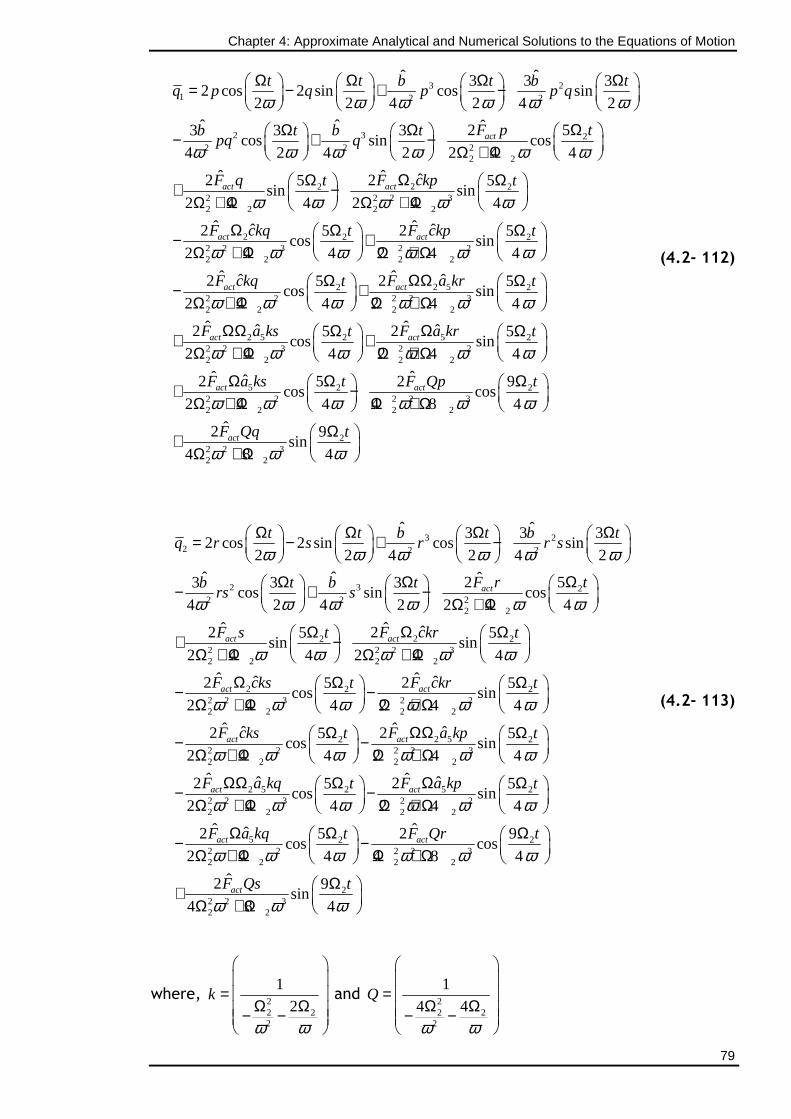
Chapter 4: Approximate Analytical and Numerical Solutions to the Equations of Motion
79
3 2
1 2 2
2 3 22 2 2
2 2
2222 2
ˆ ˆ3 3 32 cos 2 sin cos sin
2 2 4 2 4 2
ˆ ˆ ˆ2 53 3 3cos sin cos
4 2 4 2 2 4 4
ˆ ˆ ˆ2 25sin
2 4 4
ω ω ω ω ω ω
ω ω ω ω ω ω
ω ω
Ω Ω Ω Ω = − + −
ΩΩ Ω − + − Ω + Ω
ΩΩ + − Ω + Ω
act
act act
t t b t b tq p q p p q
F p tb t b tpq q
F q Ft 22 2 32 2
2 2 22 2 3 2 22 2 2 2
2 52 22 2 2 2 32 2 2 2
2 5
5sin
2 4 4
ˆ ˆˆ ˆ2 25 5cos sin
2 4 4 2 4 4
ˆ ˆˆ ˆ2 25 5cos sin
2 4 4 2 4 4
ˆ ˆ2
ω ω ω
ω ω ω ω ω ω
ω ω ω ω ω ω
Ω Ω + Ω
Ω Ω Ω − + Ω + Ω Ω + Ω
ΩΩΩ Ω − + Ω + Ω Ω + Ω
ΩΩ+
act act
act act
act
ckp t
F ckq F ckpt t
F ckq F a krt t
F a k 52 22 2 3 2 22 2 2 2
5 2 22 2 2 2 32 2 2 2
22 2 32 2
ˆ ˆ25 5cos sin
2 4 4 2 4 4
ˆ ˆˆ2 25 9cos cos
2 4 4 4 8 4
ˆ2 9sin
4 8 4
ω ω ω ω ω ω
ω ω ω ω ω ω
ω ω ω
ΩΩ Ω + Ω + Ω Ω + Ω
Ω Ω Ω + − Ω + Ω Ω + Ω
Ω + Ω + Ω
act
act act
act
s F a krt t
F a ks F Qpt t
F Qq t
(4.2- 112)
3 2
2 2 2
2 3 22 2 2
2 2
2222 2
ˆ ˆ3 3 32 cos 2 sin cos sin
2 2 4 2 4 2
ˆ ˆ ˆ2 53 3 3cos sin cos
4 2 4 2 2 4 4
ˆ ˆ ˆ2 25sin
2 4 4
ω ω ω ω ω ω
ω ω ω ω ω ω
ω ω
Ω Ω Ω Ω = − + −
ΩΩ Ω − + − Ω + Ω
ΩΩ + − Ω + Ω
act
act act
t t b t b tq r s r r s
F r tb t b trs s
F s Ft 22 2 32 2
2 2 22 2 3 2 22 2 2 2
2 52 22 2 2 2 32 2 2 2
2 5
5sin
2 4 4
ˆ ˆˆ ˆ2 25 5cos sin
2 4 4 2 4 4
ˆ ˆˆ ˆ2 25 5cos sin
2 4 4 2 4 4
ˆ ˆ2
ω ω ω
ω ω ω ω ω ω
ω ω ω ω ω ω
Ω Ω + Ω
Ω Ω Ω − − Ω + Ω Ω + Ω
ΩΩΩ Ω − − Ω + Ω Ω + Ω
ΩΩ−
act act
act act
act
ckr t
F cks F ckrt t
F cks F a kpt t
F a k 52 22 2 3 2 22 2 2 2
5 2 22 2 2 2 32 2 2 2
22 2 32 2
ˆ ˆ25 5cos sin
2 4 4 2 4 4
ˆ ˆˆ2 25 9cos cos
2 4 4 4 8 4
ˆ2 9sin
4 8 4
ω ω ω ω ω ω
ω ω ω ω ω ω
ω ω ω
ΩΩ Ω − Ω + Ω Ω + Ω
Ω Ω Ω − − Ω + Ω Ω + Ω
Ω + Ω + Ω
act
act act
act
q F a kpt t
F a kq F Qrt t
F Qs t
(4.2- 113)
where, 22 22
12
k
ω ω
= Ω Ω − −
and 22 2
2
14 4
Q
ω ω
= Ω Ω − −
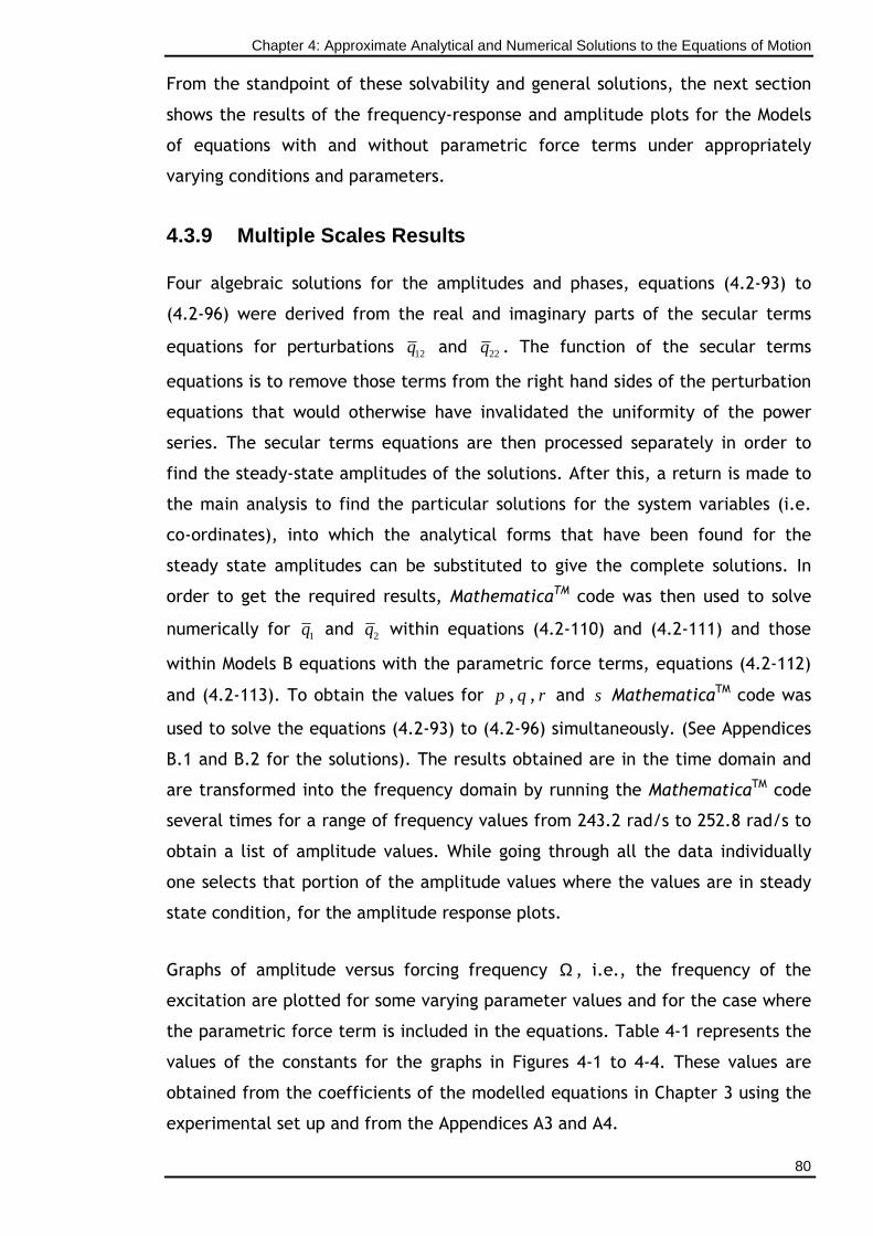
Chapter 4: Approximate Analytical and Numerical Solutions to the Equations of Motion
80
From the standpoint of these solvability and general solutions, the next section
shows the results of the frequency-response and amplitude plots for the Models
of equations with and without parametric force terms under appropriately
varying conditions and parameters.
4.3.9 Multiple Scales Results
Four algebraic solutions for the amplitudes and phases, equations (4.2-93) to
(4.2-96) were derived from the real and imaginary parts of the secular terms
equations for perturbations 12q and 22q . The function of the secular terms
equations is to remove those terms from the right hand sides of the perturbation
equations that would otherwise have invalidated the uniformity of the power
series. The secular terms equations are then processed separately in order to
find the steady-state amplitudes of the solutions. After this, a return is made to
the main analysis to find the particular solutions for the system variables (i.e.
co-ordinates), into which the analytical forms that have been found for the
steady state amplitudes can be substituted to give the complete solutions. In
order to get the required results, MathematicaTM code was then used to solve
numerically for 1q and 2q within equations (4.2-110) and (4.2-111) and those
within Models B equations with the parametric force terms, equations (4.2-112)
and (4.2-113). To obtain the values for p ,q , r and s MathematicaTM code was
used to solve the equations (4.2-93) to (4.2-96) simultaneously. (See Appendices
B.1 and B.2 for the solutions). The results obtained are in the time domain and
are transformed into the frequency domain by running the MathematicaTM code
several times for a range of frequency values from 243.2 rad/s to 252.8 rad/s to
obtain a list of amplitude values. While going through all the data individually
one selects that portion of the amplitude values where the values are in steady
state condition, for the amplitude response plots.
Graphs of amplitude versus forcing frequency Ω , i.e., the frequency of the
excitation are plotted for some varying parameter values and for the case where
the parametric force term is included in the equations. Table 4-1 represents the
values of the constants for the graphs in Figures 4-1 to 4-4. These values are
obtained from the coefficients of the modelled equations in Chapter 3 using the
experimental set up and from the Appendices A3 and A4.
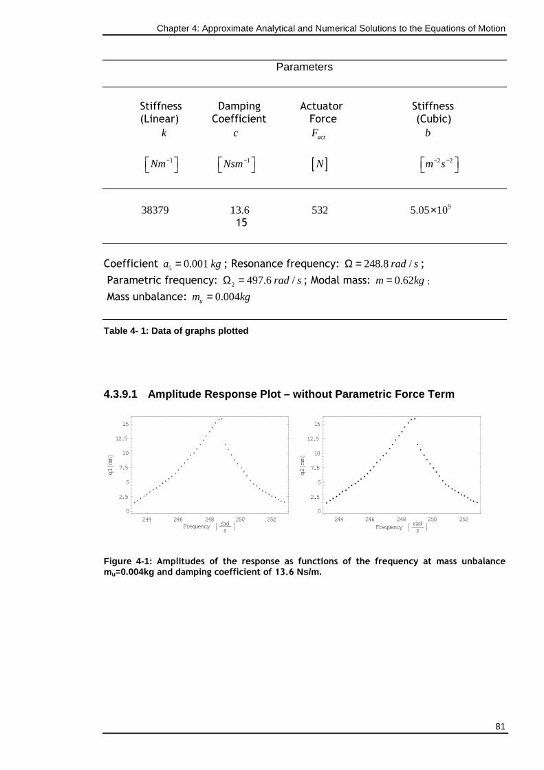
Chapter 4: Approximate Analytical and Numerical Solutions to the Equations of Motion
81
Parameters
Stiffness Damping Actuator Stiffness (Linear) Coefficient Force (Cubic) k c actF b
1Nm− 1Nsm− [ ]N 2 2m s− −
38379 13.6 532 95.05 10× 15 Coefficient 5 0.001a = kg ; Resonance frequency: 248.8 /rad sΩ = ;
Parametric frequency: 2 497.6 /rad sΩ = ; Modal mass: 0.62m kg= ;
Mass unbalance: 0.004um kg=
Table 4- 1: Data of graphs plotted
4.3.9.1 Amplitude Response Plot – without Parametri c Force Term
244 246 248 250 252Frequency A rad
sE
0
2.5
5
7.5
10
12.5
15
1q@mmD
244 246 248 250 252
Frequency A rads
E
0
2.5
5
7.5
10
12.5
15
2q@mmD
Figure 4-1: Amplitudes of the response as functions of the frequency at mass unbalance mu=0.004kg and damping coefficient of 13.6 Ns/m.
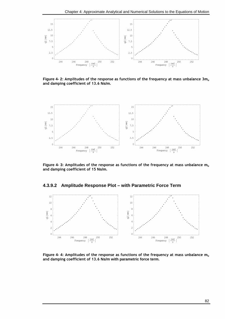
Chapter 4: Approximate Analytical and Numerical Solutions to the Equations of Motion
82
244 246 248 250 252Frequency A rad
sE
0
2.5
5
7.5
10
12.5
15
1q@mmD
244 246 248 250 252
Frequency A rads
E
0
2.5
5
7.5
10
12.5
15
2q@mm
D
Figure 4- 2: Amplitudes of the response as functions of the frequency at mass unbalance 3mu
and damping coefficient of 13.6 Ns/m.
244 246 248 250 252Frequency A rad
sE
0
2.5
5
7.5
10
12.5
15
1q
@mm
D
244 246 248 250 252
Frequency A rads
E
0
2.5
5
7.5
10
12.5
15
2q@mmD
Figure 4- 3: Amplitudes of the response as functions of the frequency at mass unbalance mu
and damping coefficient of 15 Ns/m.
4.3.9.2 Amplitude Response Plot – with Parametric F orce Term
244 246 248 250 252Frequency A rad
sE
0
2
4
6
8
10
12
1q
@mm
D
244 246 248 250 252
Frequency A rads
E
0
2
4
6
8
10
12
2q
@mmD
Figure 4- 4: Amplitudes of the response as functions of the frequency at mass unbalance mu
and damping coefficient of 13.6 Ns/m with parametric force term.
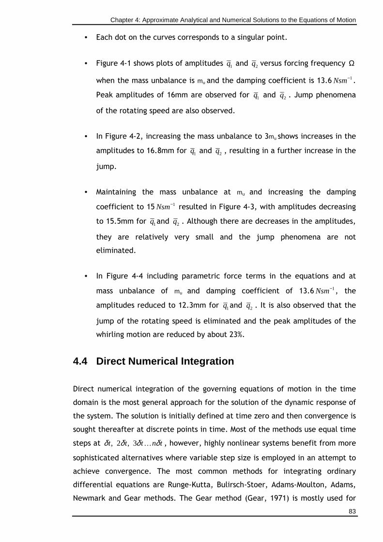
Chapter 4: Approximate Analytical and Numerical Solutions to the Equations of Motion
83
• Each dot on the curves corresponds to a singular point.
• Figure 4-1 shows plots of amplitudes 1q and 2q versus forcing frequency Ω
when the mass unbalance is mu and the damping coefficient is 13.6 1Nsm− .
Peak amplitudes of 16mm are observed for 1q and 2q . Jump phenomena
of the rotating speed are also observed.
• In Figure 4-2, increasing the mass unbalance to 3mu shows increases in the
amplitudes to 16.8mm for 1q and 2q , resulting in a further increase in the
jump.
• Maintaining the mass unbalance at mu and increasing the damping
coefficient to 15 1Nsm− resulted in Figure 4-3, with amplitudes decreasing
to 15.5mm for 1q and 2q . Although there are decreases in the amplitudes,
they are relatively very small and the jump phenomena are not
eliminated.
• In Figure 4-4 including parametric force terms in the equations and at
mass unbalance of mu and damping coefficient of 13.6 1Nsm− , the
amplitudes reduced to 12.3mm for 1q and 2q . It is also observed that the
jump of the rotating speed is eliminated and the peak amplitudes of the
whirling motion are reduced by about 23%.
4.4 Direct Numerical Integration
Direct numerical integration of the governing equations of motion in the time
domain is the most general approach for the solution of the dynamic response of
the system. The solution is initially defined at time zero and then convergence is
sought thereafter at discrete points in time. Most of the methods use equal time
steps at , 2 , 3t t t n tδ δ δ δ… , however, highly nonlinear systems benefit from more
sophisticated alternatives where variable step size is employed in an attempt to
achieve convergence. The most common methods for integrating ordinary
differential equations are Runge-Kutta, Bulirsch-Stoer, Adams-Moulton, Adams,
Newmark and Gear methods. The Gear method (Gear, 1971) is mostly used for
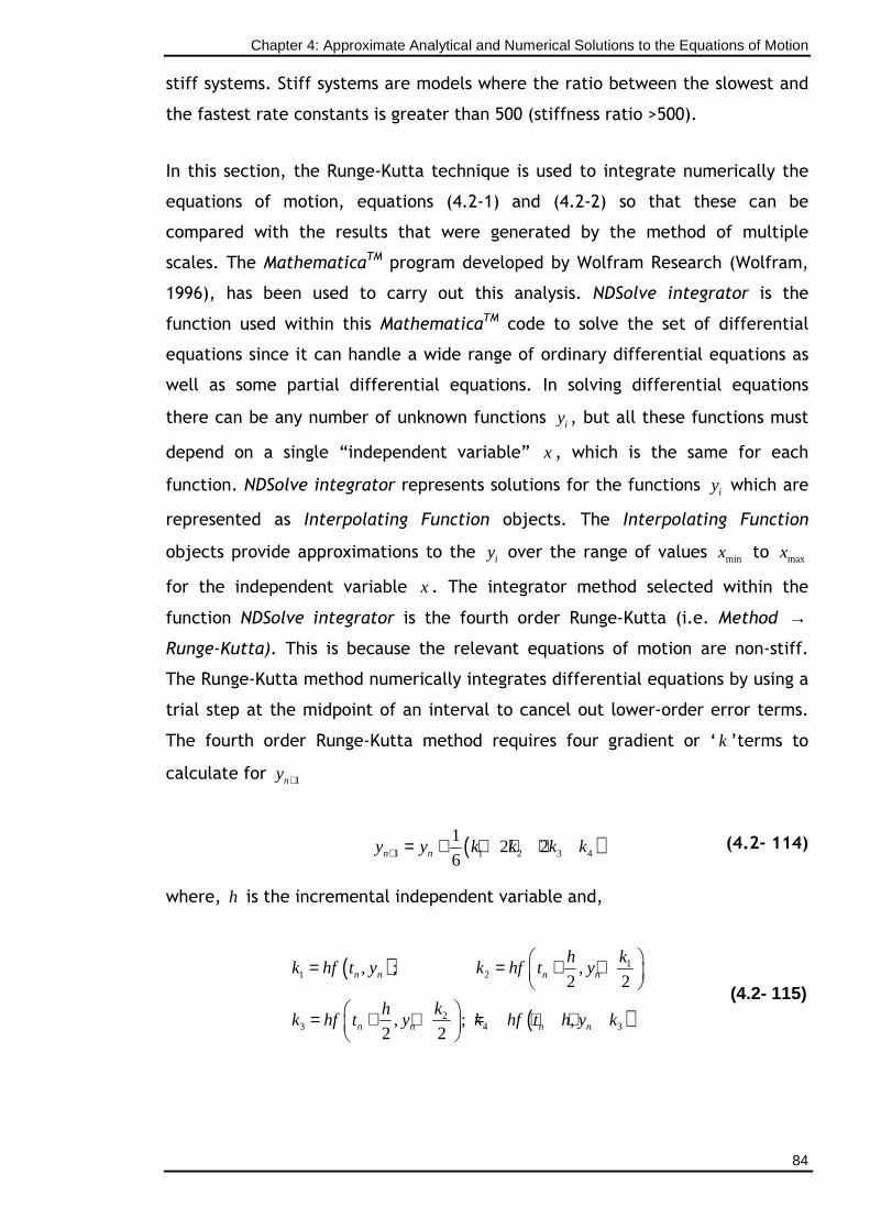
Chapter 4: Approximate Analytical and Numerical Solutions to the Equations of Motion
84
stiff systems. Stiff systems are models where the ratio between the slowest and
the fastest rate constants is greater than 500 (stiffness ratio >500).
In this section, the Runge-Kutta technique is used to integrate numerically the
equations of motion, equations (4.2-1) and (4.2-2) so that these can be
compared with the results that were generated by the method of multiple
scales. The MathematicaTM program developed by Wolfram Research (Wolfram,
1996), has been used to carry out this analysis. NDSolve integrator is the
function used within this MathematicaTM code to solve the set of differential
equations since it can handle a wide range of ordinary differential equations as
well as some partial differential equations. In solving differential equations
there can be any number of unknown functions iy , but all these functions must
depend on a single “independent variable” x , which is the same for each
function. NDSolve integrator represents solutions for the functions iy which are
represented as Interpolating Function objects. The Interpolating Function
objects provide approximations to the iy over the range of values minx to maxx
for the independent variable x . The integrator method selected within the
function NDSolve integrator is the fourth order Runge-Kutta (i.e. Method →
Runge-Kutta). This is because the relevant equations of motion are non-stiff.
The Runge-Kutta method numerically integrates differential equations by using a
trial step at the midpoint of an interval to cancel out lower-order error terms.
The fourth order Runge-Kutta method requires four gradient or ‘ k ’terms to
calculate for 1ny +
( )1 1 2 3 4
12 2
6n ny y k k k k+ = + + + + (4.2- 114)
where, h is the incremental independent variable and,
( )
( )
11 2
23 4 3
, ; ,2 2
, ; ,2 2
n n n n
n n n n
khk hf t y k hf t y
khk hf t y k hf t h y k
= = + +
= + + = + +
(4.2- 115)
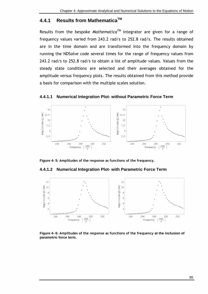
Chapter 4: Approximate Analytical and Numerical Solutions to the Equations of Motion
85
4.4.1 Results from MathematicaTM
Results from the bespoke MathematicaTM integrator are given for a range of
frequency values varied from 243.2 rad/s to 252.8 rad/s. The results obtained
are in the time domain and are transformed into the frequency domain by
running the NDSolve code several times for the range of frequency values from
243.2 rad/s to 252.8 rad/s to obtain a list of amplitude values. Values from the
steady state conditions are selected and their averages obtained for the
amplitude versus frequency plots. The results obtained from this method provide
a basis for comparison with the multiple scales solution.
4.4.1.1 Numerical Integration Plot- without Paramet ric Force Term
244 246 248 250 252Frequency A rad
sE
2.5
5
7.5
10
12.5
15
edutilpmA
1q@mmD
244 246 248 250 252
Frequency A rads
E
2.5
5
7.5
10
12.5
15
edutilpmA
2q@mmD
Figure 4- 5: Amplitudes of the response as functions of the frequency.
4.4.1.2 Numerical Integration Plot- with Parametric Force Term
244 246 248 250 252Frequency A rad
sE
2
4
6
8
10
12
edutilpmA
1q@mmD
244 246 248 250 252
Frequency A rads
E
2
4
6
8
10
12
edutilpmA
2q@mmD
Figure 4- 6: Amplitudes of the response as functions of the frequency at the inclusion of parametric force term.
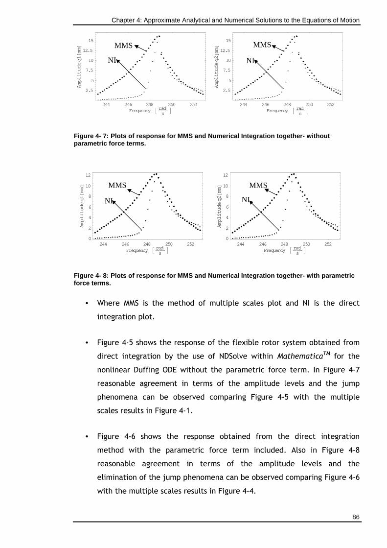
Chapter 4: Approximate Analytical and Numerical Solutions to the Equations of Motion
86
244 246 248 250 252Frequency A rad
sE
2.5
5
7.5
10
12.5
15
edutilpmA
1q@mmD
244 246 248 250 252
Frequency A rads
E
2.5
5
7.5
10
12.5
15
edutilpmA
2q@mmD
Figure 4- 7: Plots of response for MMS and Numerica l Integration together- without parametric force terms.
244 246 248 250 252Frequency A rad
sE
0
2
4
6
8
10
12
edutilpmA
1q@mmD
244 246 248 250 252
Frequency A rads
E
0
2
4
6
8
10
12
edutilpmA
2q@mmD
Figure 4- 8: Plots of response for MMS and Numerica l Integration together- with parametric force terms.
• Where MMS is the method of multiple scales plot and NI is the direct
integration plot.
• Figure 4-5 shows the response of the flexible rotor system obtained from
direct integration by the use of NDSolve within MathematicaTM for the
nonlinear Duffing ODE without the parametric force term. In Figure 4-7
reasonable agreement in terms of the amplitude levels and the jump
phenomena can be observed comparing Figure 4-5 with the multiple
scales results in Figure 4-1.
• Figure 4-6 shows the response obtained from the direct integration
method with the parametric force term included. Also in Figure 4-8
reasonable agreement in terms of the amplitude levels and the
elimination of the jump phenomena can be observed comparing Figure 4-6
with the multiple scales results in Figure 4-4.
MMS MMS
MMS MMS
NI NI
NI NI
Chapter 4: Approximate Analytical and Numerical Solutions to the Equations of Motion
87
4.5 Discussion of Results
Comparison between the results from the multiple scales analysis and the
numerical integration benchmark summarised here shows evidence of a
consistent phenomenon whereby both the responses in the first mode of 1q and
2q show hardening characteristics, jump phenomena and both stable and
unstable solutions when the equations of motion contain no parametric force
term. Including the parametric force terms, the two solutions show decreases in
amplitude values, elimination of the jump phenomena and stable solutions.
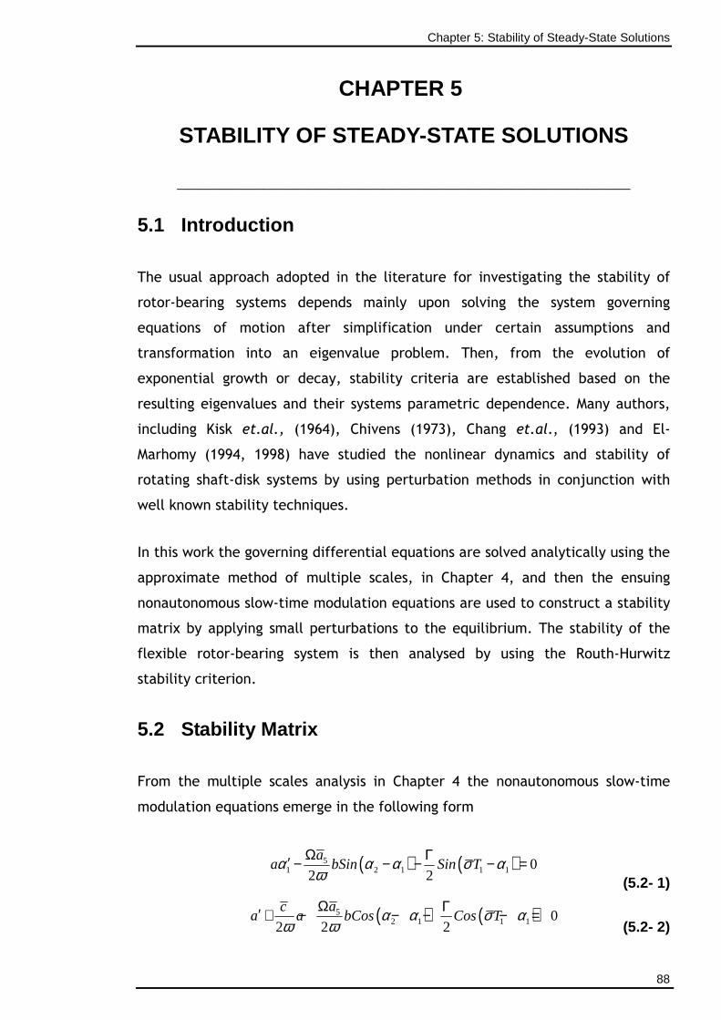
Chapter 5: Stability of Steady-State Solutions
88
CHAPTER 5
STABILITY OF STEADY-STATE SOLUTIONS
__________________________________________
5.1 Introduction
The usual approach adopted in the literature for investigating the stability of
rotor-bearing systems depends mainly upon solving the system governing
equations of motion after simplification under certain assumptions and
transformation into an eigenvalue problem. Then, from the evolution of
exponential growth or decay, stability criteria are established based on the
resulting eigenvalues and their systems parametric dependence. Many authors,
including Kisk et.al., (1964), Chivens (1973), Chang et.al., (1993) and El-
Marhomy (1994, 1998) have studied the nonlinear dynamics and stability of
rotating shaft-disk systems by using perturbation methods in conjunction with
well known stability techniques.
In this work the governing differential equations are solved analytically using the
approximate method of multiple scales, in Chapter 4, and then the ensuing
nonautonomous slow-time modulation equations are used to construct a stability
matrix by applying small perturbations to the equilibrium. The stability of the
flexible rotor-bearing system is then analysed by using the Routh-Hurwitz
stability criterion.
5.2 Stability Matrix
From the multiple scales analysis in Chapter 4 the nonautonomous slow-time
modulation equations emerge in the following form
( ) ( )51 2 1 1 1 0
2 2
aa bSin Sin Tα α α σ α
ωΩ Γ′ − − − − =
(5.2- 1) ( ) ( )5
2 1 1 1 02 2 2
aca a bCos Cos Tα α σ α
ω ωΩ Γ′ + − − − − =
(5.2- 2)
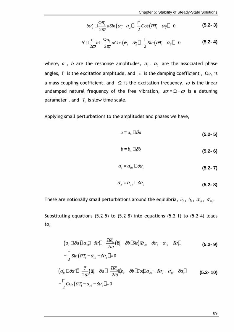
Chapter 5: Stability of Steady-State Solutions
89
( ) ( )52 1 2 1 2 0
2 2
ab aSin Cos Tα α α σ α
ωΩ Γ′ + − + − = (5.2- 3)
( ) ( )51 2 1 2 0
2 2 2
acb b aCos Sin Tα α σ α
ω ωΩ Γ′ + + − − − = (5.2- 4)
where, a , b are the response amplitudes, 1α , 2α are the associated phase
angles, Γ is the excitation amplitude, and c is the damping coefficient , 5aΩ is
a mass coupling coefficient, and Ω is the excitation frequency, ω is the linear
undamped natural frequency of the free vibration, εσ ω= Ω − is a detuning
parameter , and 1T is slow time scale.
Applying small perturbations to the amplitudes and phases we have,
0a a aδ= + (5.2- 5)
0b b bδ= + (5.2- 6)
1 10 1α α δα= + (5.2- 7)
2 20 2α α δα= + (5.2- 8)
These are notionally small perturbations around the equilibria, 0a , 0b , 10α , 20α .
Substituting equations (5.2-5) to (5.2-8) into equations (5.2-1) to (5.2-4) leads
to,
( ) ( ) ( ) ( )
( )
50 10 1 0 20 2 10 1
1 10 1
2
02
aa a b b Sin
Sin T
δ α δα δ α δα α δαω
σ α δα
Ω′ ′+ + − + + − −
Γ− − − =
(5.2- 9)
( ) ( ) ( ) ( )
( )
50 0 0 20 2 10 1
1 10 1
2 2
02
aca a b b Cos
Cos T
α δα δ δ α δα α δαω ω
σ α δα
Ω′ ′+ + + − + + − −
Γ− − − =
(5.2- 10)
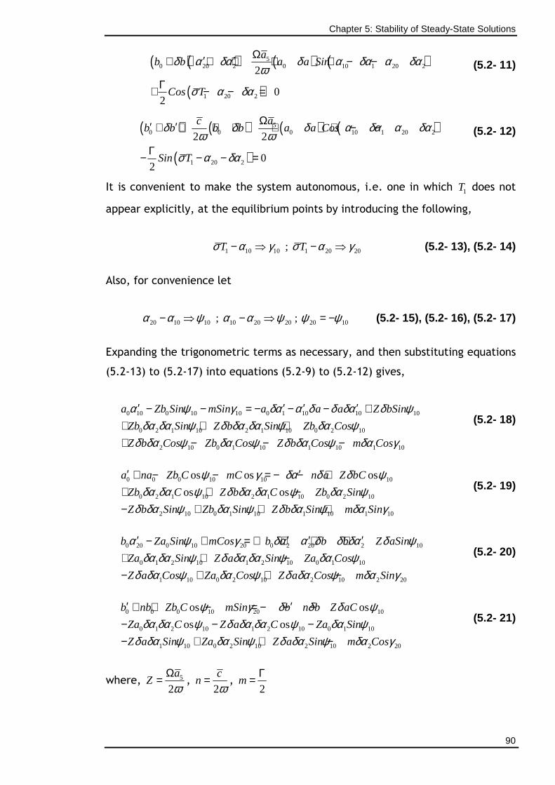
Chapter 5: Stability of Steady-State Solutions
90
( )( ) ( ) ( )
( )
50 20 2 0 10 1 20 2
1 20 2
2
02
ab b a a Sin
Cos T
δ α δα δ α δα α δαω
σ α δα
Ω′ ′+ + + + + − −
Γ+ − − =
(5.2- 11)
( ) ( ) ( ) ( )
( )
50 0 0 10 1 20 2
1 20 2
2 2
02
acb b b b a a Cos
Sin T
δ δ δ α δα α δαω ω
σ α δα
Ω′ ′+ + + + + + − −
Γ− − − =
(5.2- 12)
It is convenient to make the system autonomous, i.e. one in which 1T does not
appear explicitly, at the equilibrium points by introducing the following,
1 10 10 1 20 20;T Tσ α γ σ α γ− ⇒ − ⇒ (5.2- 13), (5.2- 14)
Also, for convenience let
20 10 10 10 20 20 20 10; ;α α ψ α α ψ ψ ψ− ⇒ − ⇒ = − (5.2- 15), (5.2- 16), (5.2- 17)
Expanding the trigonometric terms as necessary, and then substituting equations
(5.2-13) to (5.2-17) into equations (5.2-9) to (5.2-12) gives,
0 10 0 10 10 0 1 10 10 10
0 2 1 10 2 1 10 0 2 10
2 10 0 1 10 1 10 1 10
a Zb Sin mSin a a a Z bSin
Zb Sin Z b Sin Zb Cos
Z b Cos Zb Cos Z b Cos m Cos
α ψ γ δα α δ δ δα δ ψδα δα ψ δ δα δα ψ δα ψ
δ δα ψ δα ψ δ δα ψ δα γ
′ ′ ′ ′− − = − − − ++ + ++ − − −
(5.2- 18)
0 0 0 10 10 10
0 2 1 10 2 1 10 0 2 10
2 10 0 1 10 1 10 1 10
os os os
os os
a na Zb C mC n a Z bC
Zb C Z b C Zb Sin
Z b Sin Zb Sin Z b Sin m Sin
ψ γ δα δ δ ψδα δα ψ δ δα δα ψ δα ψ
δ δα ψ δα ψ δ δα ψ δα γ
′ ′+ − − = − − ++ + −− + + +
(5.2- 19)
0 20 0 10 20 0 2 20 2 10
0 1 2 10 1 2 10 0 1 10
1 10 0 2 10 2 10 2 20
b Za Sin mCos b b b Z aSin
Za Sin Z a Sin Za Cos
Z a Cos Za Cos Z a Cos m Sin
α ψ γ δα α δ δ δα δ ψδα δα ψ δ δα δα ψ δα ψ
δ δα ψ δα ψ δ δα ψ δα γ
′ ′ ′ ′− + = + + + ++ + −− + + −
(5.2- 20)
0 0 0 10 20 10
0 1 2 10 1 2 10 0 1 10
1 10 0 2 10 2 10 2 20
os os
os os
b nb Zb C mSin b n b Z aC
Za C Z a C Za Sin
Z a Sin Za Sin Z a Sin m Cos
ψ γ δ δ δ ψδα δα ψ δ δα δα ψ δα ψ
δ δα ψ δα ψ δ δα ψ δα γ
′ ′+ + − = − − −− − −− + + −
(5.2- 21)
where, 5
2
aZ
ωΩ= ,
2
cn
ω= ,
2m
Γ=
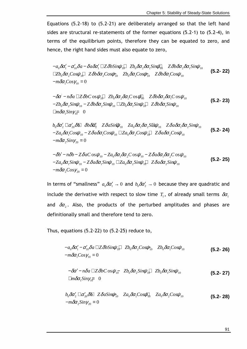
Chapter 5: Stability of Steady-State Solutions
91
Equations (5.2-18) to (5.2-21) are deliberately arranged so that the left hand
sides are structural re-statements of the former equations (5.2-1) to (5.2-4), in
terms of the equilibrium points, therefore they can be equated to zero, and
hence, the right hand sides must also equate to zero,
0 1 10 1 10 0 2 1 10 2 1 10
0 2 10 2 10 0 1 10 1 10
1 10 0
a a a Z bSin Zb Sin Z b Sin
Zb Cos Z b Cos Zb Cos Z b Cos
m Cos
δα α δ δ δα δ ψ δα δα ψ δ δα δα ψδα ψ δ δα ψ δα ψ δ δα ψ
δα γ
′ ′ ′− − − + + ++ + − −− =
(5.2- 22)
'10 0 2 1 10 2 1 10
0 2 10 2 10 0 1 10 1 10
1 10
os os os
0
n a Z bC Zb C Z b C
Zb Sin Z b Sin Zb Sin Z b Sin
m Sin
δα δ δ ψ δα δα ψ δ δα δα ψδα ψ δ δα ψ δα ψ δ δα ψ
δα γ
− − + + +− − + ++ =
(5.2- 23)
0 2 20 2 10 0 1 2 10 1 2 10
0 1 10 1 10 0 2 10 2 10
2 20 0
b b b Z aSin Za Sin Z a Sin
Za Cos Z a Cos Za Cos Z a Cos
m Sin
δα α δ δ δα δ ψ δα δα ψ δ δα δα ψδα ψ δ δα ψ δα ψ δ δα ψ
δα γ
′ ′ ′+ + + + +− − + +− =
(5.2- 24)
10 0 1 2 10 1 2 10
0 1 10 1 10 0 2 10 2 10
2 20
os os os
0
b n b Z aC Za C Z a C
Za Sin Z a Sin Za Sin Z a Sin
m Cos
δ δ δ ψ δα δα ψ δ δα δα ψδα ψ δ δα ψ δα ψ δ δα ψ
δα γ
′− − − − −− − + +− =
(5.2- 25)
In terms of “smallness” 0 1 0a δα ′ → and 0 2 0b δα ′ → because they are quadratic and
include the derivative with respect to slow time 1T , of already small terms 1δα
and 2δα . Also, the products of the perturbed amplitudes and phases are
definitionally small and therefore tend to zero.
Thus, equations (5.2-22) to (5.2-25) reduce to,
0 1 10 10 0 2 10 0 1 10
1 10 0
a a Z bSin Zb Cos Zb Cos
m Cos
δα α δ δ ψ δα ψ δα ψδα γ
′ ′− − + + −− =
(5.2- 26)
10 0 2 10 0 1 10
1 10
os
0
n a Z bC Zb Sin Zb Sin
m Sin
δα δ δ ψ δα ψ δα ψδα γ′− − + − +
+ = (5.2- 27)
0 2 20 10 0 1 10 0 2 10
2 20 0
b b Z aSin Za Cos Za Cos
m Sin
δα α δ δ ψ δα ψ δα ψδα γ
′ ′+ + − +− =
(5.2- 28)
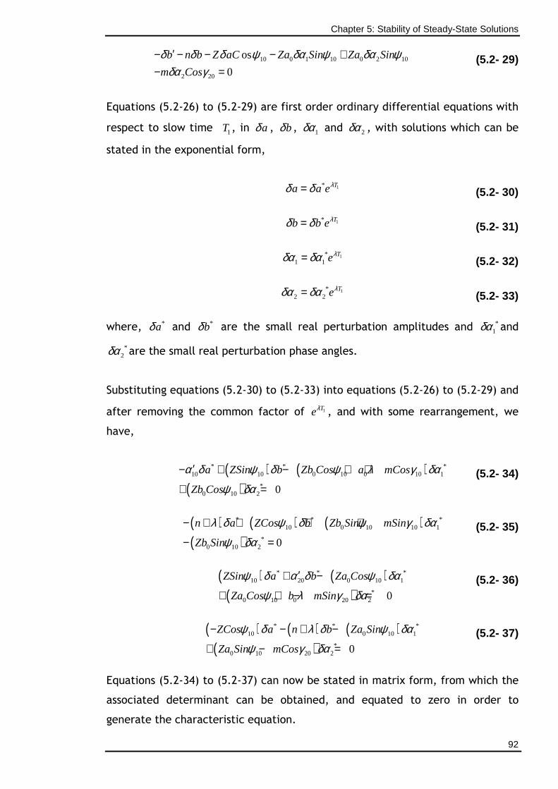
Chapter 5: Stability of Steady-State Solutions
92
10 0 1 10 0 2 10
2 20
os
0
b n b Z aC Za Sin Za Sin
m Cos
δ δ δ ψ δα ψ δα ψδα γ′− − − − +
− = (5.2- 29)
Equations (5.2-26) to (5.2-29) are first order ordinary differential equations with
respect to slow time 1T , in aδ , bδ , 1δα and 2δα , with solutions which can be
stated in the exponential form,
1* Ta a eλδ δ= (5.2- 30)
1* Tb b eλδ δ= (5.2- 31)
1*1 1
Teλδα δα= (5.2- 32)
1*2 2
Teλδα δα= (5.2- 33)
where, *aδ and *bδ are the small real perturbation amplitudes and *1δα and
*2δα are the small real perturbation phase angles.
Substituting equations (5.2-30) to (5.2-33) into equations (5.2-26) to (5.2-29) and
after removing the common factor of 1Teλ , and with some rearrangement, we
have,
( ) ( )( )
* * *10 10 0 10 0 10 1
*0 10 2 0
a ZSin b Zb Cos a mCos
Zb Cos
α δ ψ δ ψ λ γ δα
ψ δα
′− + − + +
+ = (5.2- 34)
( ) ( ) ( )( )
* * *10 0 10 10 1
*0 10 2 0
n a ZCos b Zb Sin mSin
Zb Sin
λ δ ψ δ ψ γ δα
ψ δα
− + + + +
− = (5.2- 35)
( ) ( )( )
* * *10 20 0 10 1
*0 10 0 20 2 0
ZSin a b Za Cos
Za Cos b mSin
ψ δ α δ ψ δα
ψ λ γ δα
′+ −
+ + − = (5.2- 36)
( ) ( ) ( )( )
* * *10 0 10 1
*0 10 20 2 0
ZCos a n b Za Sin
Za Sin mCos
ψ δ λ δ ψ δα
ψ γ δα
− − + −
+ − = (5.2- 37)
Equations (5.2-34) to (5.2-37) can now be stated in matrix form, from which the
associated determinant can be obtained, and equated to zero in order to
generate the characteristic equation.
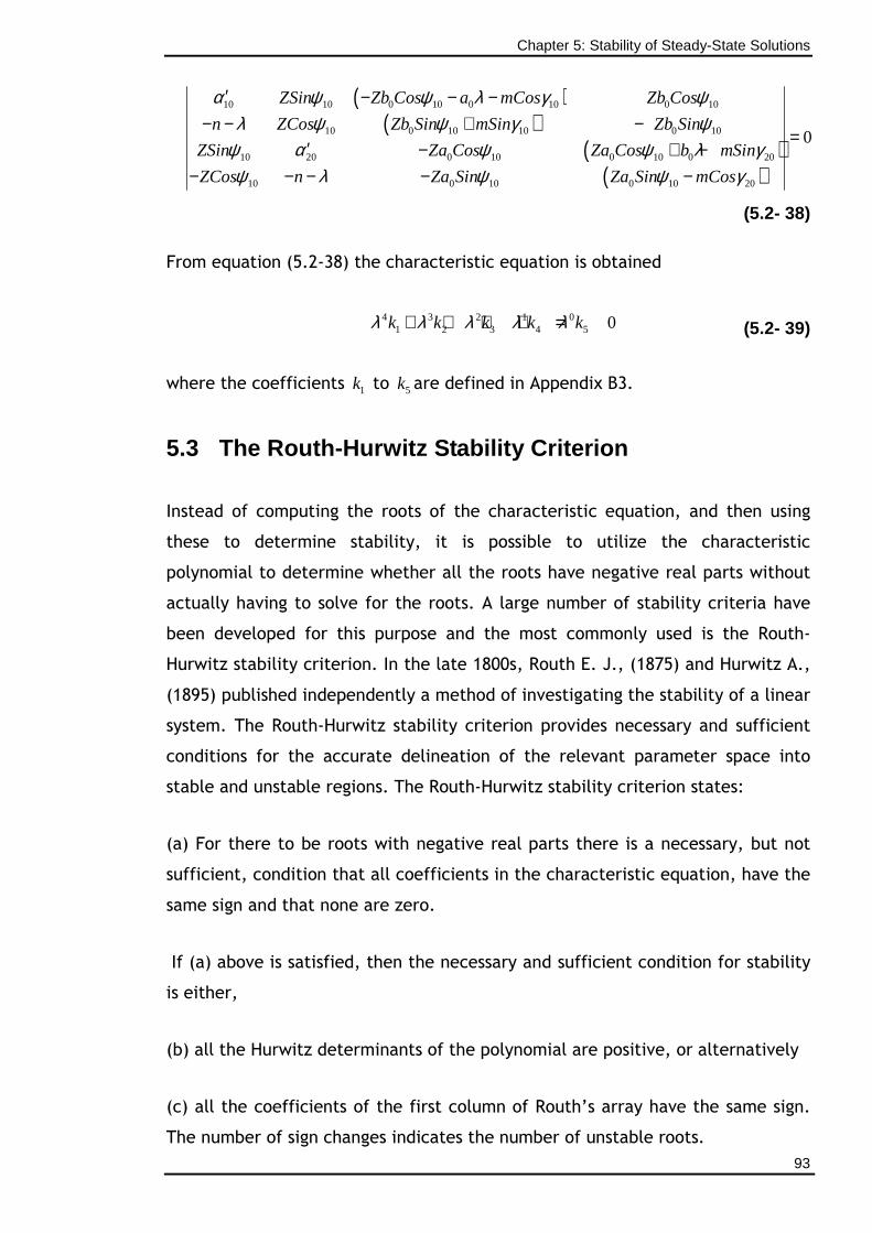
Chapter 5: Stability of Steady-State Solutions
93
( )( )
( )( )
10 10 0 10 0 10 0 10
10 0 10 10 0 10
10 20 0 10 0 10 0 20
10 0 10 0 10 20
0
ZSin Zb Cos a mCos Zb Cos
n ZCos Zb Sin mSin Zb Sin
ZSin Za Cos Za Cos b mSin
ZCos n Za Sin Za Sin mCos
α ψ ψ λ γ ψλ ψ ψ γ ψ
ψ α ψ ψ λ γψ λ ψ ψ γ
′ − − −− − + −
=′ − + −
− − − − −
(5.2- 38)
From equation (5.2-38) the characteristic equation is obtained
4 3 2 1 01 2 3 4 5 0k k k k kλ λ λ λ λ+ + + + = (5.2- 39)
where the coefficients 1k to 5k are defined in Appendix B3.
5.3 The Routh-Hurwitz Stability Criterion
Instead of computing the roots of the characteristic equation, and then using
these to determine stability, it is possible to utilize the characteristic
polynomial to determine whether all the roots have negative real parts without
actually having to solve for the roots. A large number of stability criteria have
been developed for this purpose and the most commonly used is the Routh-
Hurwitz stability criterion. In the late 1800s, Routh E. J., (1875) and Hurwitz A.,
(1895) published independently a method of investigating the stability of a linear
system. The Routh-Hurwitz stability criterion provides necessary and sufficient
conditions for the accurate delineation of the relevant parameter space into
stable and unstable regions. The Routh-Hurwitz stability criterion states:
(a) For there to be roots with negative real parts there is a necessary, but not
sufficient, condition that all coefficients in the characteristic equation, have the
same sign and that none are zero.
If (a) above is satisfied, then the necessary and sufficient condition for stability
is either,
(b) all the Hurwitz determinants of the polynomial are positive, or alternatively
(c) all the coefficients of the first column of Routh’s array have the same sign.
The number of sign changes indicates the number of unstable roots.
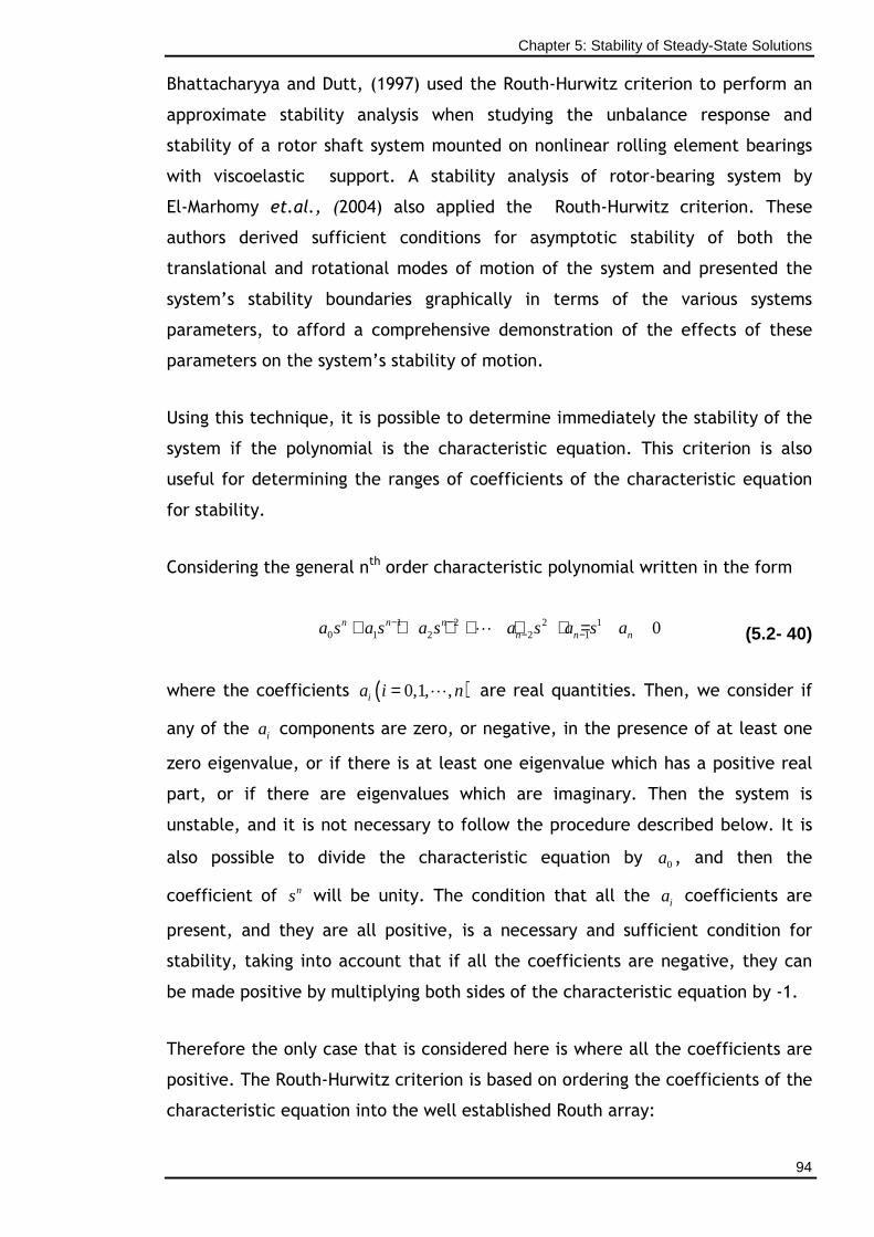
Chapter 5: Stability of Steady-State Solutions
94
Bhattacharyya and Dutt, (1997) used the Routh-Hurwitz criterion to perform an
approximate stability analysis when studying the unbalance response and
stability of a rotor shaft system mounted on nonlinear rolling element bearings
with viscoelastic support. A stability analysis of rotor-bearing system by
El-Marhomy et.al., (2004) also applied the Routh-Hurwitz criterion. These
authors derived sufficient conditions for asymptotic stability of both the
translational and rotational modes of motion of the system and presented the
system’s stability boundaries graphically in terms of the various systems
parameters, to afford a comprehensive demonstration of the effects of these
parameters on the system’s stability of motion.
Using this technique, it is possible to determine immediately the stability of the
system if the polynomial is the characteristic equation. This criterion is also
useful for determining the ranges of coefficients of the characteristic equation
for stability.
Considering the general nth order characteristic polynomial written in the form
1 2 2 10 1 2 2 1 0n n n
n n na s a s a s a s a s a− −− −+ + + + + + =⋯ (5.2- 40)
where the coefficients ( )0,1, ,ia i n= ⋯ are real quantities. Then, we consider if
any of the ia components are zero, or negative, in the presence of at least one
zero eigenvalue, or if there is at least one eigenvalue which has a positive real
part, or if there are eigenvalues which are imaginary. Then the system is
unstable, and it is not necessary to follow the procedure described below. It is
also possible to divide the characteristic equation by 0a , and then the
coefficient of ns will be unity. The condition that all the ia coefficients are
present, and they are all positive, is a necessary and sufficient condition for
stability, taking into account that if all the coefficients are negative, they can
be made positive by multiplying both sides of the characteristic equation by -1.
Therefore the only case that is considered here is where all the coefficients are
positive. The Routh-Hurwitz criterion is based on ordering the coefficients of the
characteristic equation into the well established Routh array:
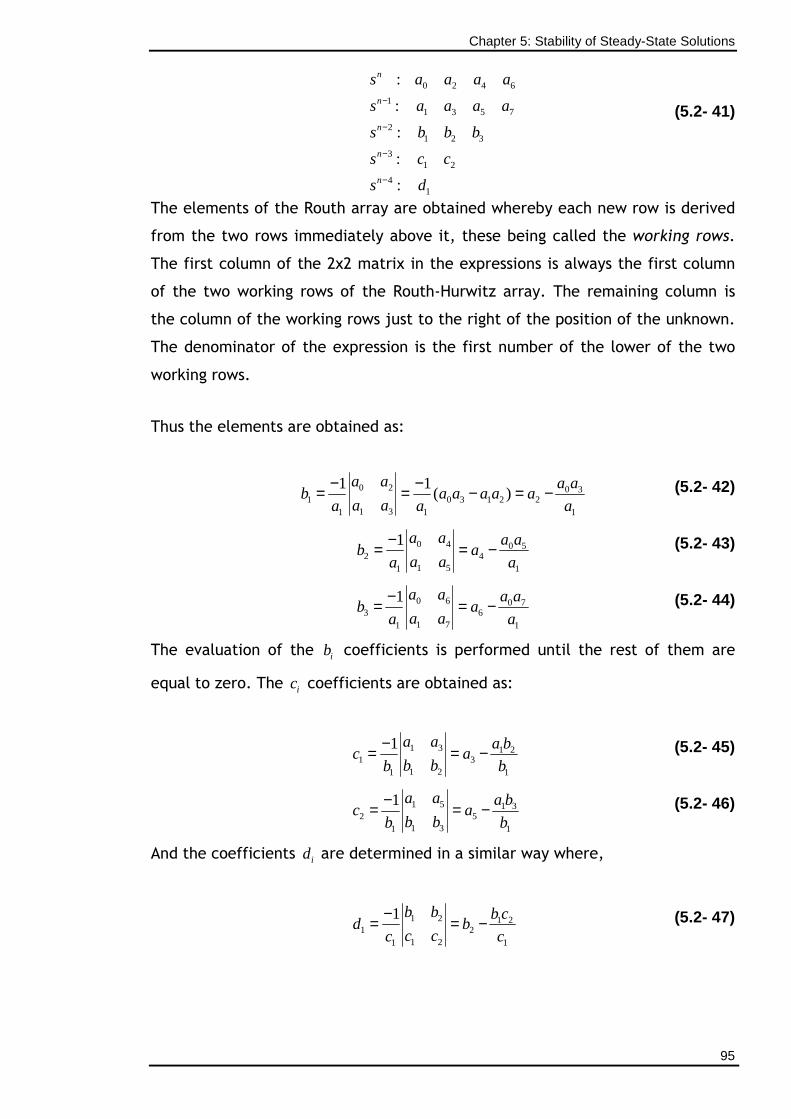
Chapter 5: Stability of Steady-State Solutions
95
0 2 4 6
11 3 5 7
21 2 3
31 2
41
:
:
:
:
:
n
n
n
n
n
s a a a a
s a a a a
s b b b
s c c
s d
−
−
−
−
(5.2- 41)
The elements of the Routh array are obtained whereby each new row is derived
from the two rows immediately above it, these being called the working rows.
The first column of the 2x2 matrix in the expressions is always the first column
of the two working rows of the Routh-Hurwitz array. The remaining column is
the column of the working rows just to the right of the position of the unknown.
The denominator of the expression is the first number of the lower of the two
working rows.
Thus the elements are obtained as:
0 2 0 3
1 0 3 1 2 21 31 1 1
1 1( )
a a a ab a a a a a
a aa a a
− −= = − = − (5.2- 42)
0 4 0 5
2 41 51 1
1 a a a ab a
a aa a
−= = − (5.2- 43)
0 6 0 7
3 61 71 1
1 a a a ab a
a aa a
−= = − (5.2- 44)
The evaluation of the ib coefficients is performed until the rest of them are
equal to zero. The ic coefficients are obtained as:
1 3 1 2
1 31 21 1
1 a a a bc a
b bb b
−= = − (5.2- 45)
1 5 1 3
2 51 31 1
1 a a a bc a
b bb b
−= = − (5.2- 46)
And the coefficients id are determined in a similar way where,
1 2 1 2
1 21 21 1
1 b b b cd b
c cc c
−= = − (5.2- 47)
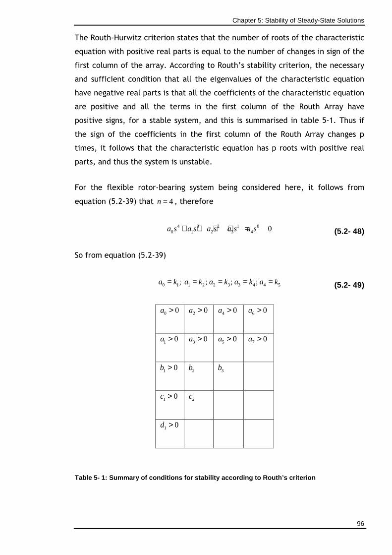
Chapter 5: Stability of Steady-State Solutions
96
The Routh-Hurwitz criterion states that the number of roots of the characteristic
equation with positive real parts is equal to the number of changes in sign of the
first column of the array. According to Routh’s stability criterion, the necessary
and sufficient condition that all the eigenvalues of the characteristic equation
have negative real parts is that all the coefficients of the characteristic equation
are positive and all the terms in the first column of the Routh Array have
positive signs, for a stable system, and this is summarised in table 5-1. Thus if
the sign of the coefficients in the first column of the Routh Array changes p
times, it follows that the characteristic equation has p roots with positive real
parts, and thus the system is unstable.
For the flexible rotor-bearing system being considered here, it follows from
equation (5.2-39) that 4n = , therefore
4 3 2 1 00 1 2 3 4 0a s a s a s a s a s+ + + + = (5.2- 48)
So from equation (5.2-39)
0 1 1 2 2 3 3 4 4 5; ; ; ;a k a k a k a k a k= = = = = (5.2- 49)
0 0a > 2 0a > 4 0a > 6 0a >
1 0a > 3 0a > 5 0a > 7 0a >
1 0b > 2b 3b
1 0c > 2c
1 0d >
Table 5- 1: Summary of conditions for stability acc ording to Routh’s criterion
Chapter 5: Stability of Steady-State Solutions
97
Hence, equations (5.2-42) to (5.2-47) can be re-stated as,
1 41 3
2
k kb k
k= − (5.2- 50)
( )12 5 5
2
0kb k k
k= − = (5.2- 51)
3 0 0 0b = − = (5.2- 52)
2 51 4
1
k kc k
b= − (5.2- 53)
( )22
1
00 0
kc
b= − = (5.2- 54)
( )11 2 2
1
0bd b b
c= − = (5.2- 55)
Therefore the elements of the first column of the Routh Array are
0 1a k= , 1 2a k= , 1 41 3
2
k kb k
k= − , 2 5
1 4
1 43
2
k kc k
k kk
k
= −
−
,and 1 5d k= .
The Routh-Hurwitz criterion requires that all the first column elements are
positive and all 0ia > , i.e. 1 0k > , 2 0k > , 3 0k > , 4 0k > , 5 0k > , 1 43
2
0k k
kk
− > , and
2 54
1 43
2
0k k
kk k
kk
− >
−
for stability.
5.3.1 Stability Results
The results of the stability of the steady-state solutions at various mass
unbalance values of the flexible rotor-bearing system are presented in Table 5-2
and Figures 5-1 and 5-2. The results show that there are values of mass
unbalance for which the system can be stable or unstable. Table 5-2 shows
discrete mass unbalance values with their coefficient values and eigenvalues.
Chapter 5: Stability of Steady-State Solutions
98
For a mass unbalance of 0.004um kg= , all first column elements are greater than
zero, and all 0ia > , i.e. 1 0.000256k = , 2 0.077k = , 3 1.5k = , 4 7.84k = , 5 0.16k = ,
1 1.47b = , 1 7.839c = , 1 0.16d = . Also the eigenvalues have negative real parts
indicating stable motion.
At mass unbalances of 3 um , 4 um and 5 um all the first column elements and ia
are greater than zero, except 5k and 1d which are less than zero, and since
1 5d k= , and with eigenvalues 4λ being real but positive, the motion is unstable.
A further increase in mass unbalance to 6 um and 7 um shows their respective
5k and 1d values to be greater than zero, and all eigenvalues as real and negative
indicating stability at these values.
Figures 5-1 and 5-2 show stability graphs of coefficients and mass unbalance,
and eigenvalues and mass unbalance, with Figures 5-1(b) and 5-2(b) showing
enlarged views of coefficients 5k and mass unbalance, and eigenvalues 4λ and
mass unbalance plots respectively, and they show the transitions between
stability and instability.
From Figures 5-1 and 5-2, at mass unbalance values between zero and 0.006kg,
all the coefficients 1k to 5k values are greater than zero and there are no sign
changes in the first columns of the Routh arrays. Also all the eigenvalues 1λ to
4λ are negative indicating stable motions.
At mass unbalance values from 0.006kg to 0.022kg, the system is unstable. The
coefficients 1k to 4k values are greater than zero, but 5k values are negative,
also negative numbers are found in the first columns of the Routh arrays,
meaning there are sign changes in the first column. The eigenvalues 4λ are either
zero or positive.
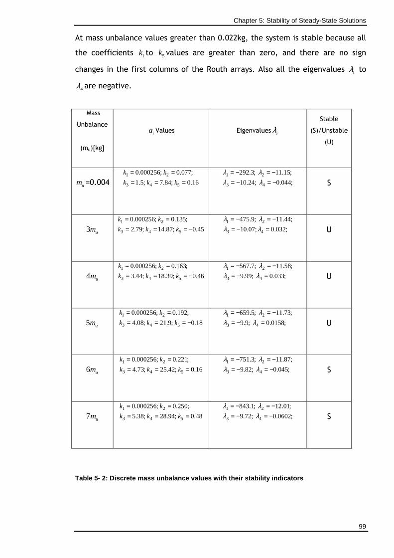
Chapter 5: Stability of Steady-State Solutions
99
At mass unbalance values greater than 0.022kg, the system is stable because all
the coefficients 1k to 5k values are greater than zero, and there are no sign
changes in the first columns of the Routh arrays. Also all the eigenvalues 1λ to
4λ are negative.
Mass
Unbalance
(mu)[kg]
ia Values Eigenvalues iλ
Stable
(S)/Unstable
(U)
um =0.004 1 2
3 4 5
0.000256; 0.077;
1.5; 7.84; 0.16
k k
k k k
= == = =
1 2
3 4
292.3; 11.15;
10.24; 0.044;
λ λλ λ
= − = −= − = − S
3 um 1 2
3 4 5
0.000256; 0.135;
2.79; 14.87; 0.45
k k
k k k
= == = = −
1 2
3 4
475.9; 11.44;
10.07; 0.032;
λ λλ λ
= − = −= − = U
4 um 1 2
3 4 5
0.000256; 0.163;
3.44; 18.39; 0.46
k k
k k k
= == = = −
1 2
3 4
567.7; 11.58;
9.99; 0.033;
λ λλ λ
= − = −= − = U
5 um 1 2
3 4 5
0.000256; 0.192;
4.08; 21.9; 0.18
k k
k k k
= == = = −
1 2
3 4
659.5; 11.73;
9.9; 0.0158;
λ λλ λ
= − = −= − = U
6 um 1 2
3 4 5
0.000256; 0.221;
4.73; 25.42; 0.16
k k
k k k
= == = =
1 2
3 4
751.3; 11.87;
9.82; 0.045;
λ λλ λ
= − = −= − = − S
7 um 1 2
3 4 5
0.000256; 0.250;
5.38; 28.94; 0.48
k k
k k k
= == = =
1 2
3 4
843.1; 12.01;
9.72; 0.0602;
λ λλ λ
= − = −= − = − S
Table 5- 2: Discrete mass unbalance values with the ir stability indicators

Chapter 5: Stability of Steady-State Solutions
100
-5
0
5
10
15
20
25
30
0 0.005 0.01 0.015 0.02 0.025 0.03
Mass Unbalance
Coe
ffici
ents
K1
K2
K3
K4
K5
(a)Combined plots for k values
K5
-0.6
-0.5
-0.4
-0.3
-0.2
-0.1
0
0.1
0.2
0 0.005 0.01 0.015 0.02 0.025 0.03
Mass Unbalance
Coe
ffici
ents
K5
(b) Enlarged view of k5 values
Figure 5- 1: Stability plots for k values
Unstable
Stable Stable
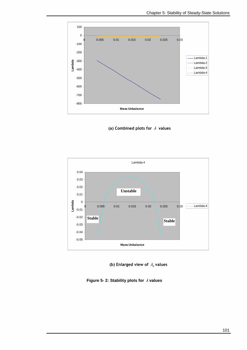
Chapter 5: Stability of Steady-State Solutions
101
-800
-700
-600
-500
-400
-300
-200
-100
0
100
0 0.005 0.01 0.015 0.02 0.025 0.03
Mass Unbalance
Lam
bda
Lambda-1
Lambda-2
Lambda-3
Lambda-4
(a) Combined plots for λ values
Lambda-4
-0.05
-0.04
-0.03
-0.02
-0.01
0
0.01
0.02
0.03
0.04
0 0.005 0.01 0.015 0.02 0.025 0.03
Mass Unbalance
Lam
bda
Lambda-4
(b) Enlarged view of 4λ values
Figure 5- 2: Stability plots for λ values
Unstable
Stable Stable
Chapter 6: Investigations of Systems Dynamics
102
CHAPTER 6
INVESTIGATION OF SYSTEMS DYNAMICS
_________________________________________________
6.1 Introduction
In nonlinear dynamical systems analysis, exact solutions are hard, if not
impossible to find. In addition to relying on analytical solutions for the flexible
rotor, emphasis can also be placed on its qualitative behaviour. The analysis
methods employed in this study are inclusive of the dynamic trajectories of the
rotor, displacement-time plots, Poincaré maps, and bifurcation diagrams.
Maximum Lyapunov exponent analysis is also used, together with the above
mentioned feature properties to determine the onset conditions for chaotic
motion. If a system falls into a chaotic regime, its behaviour is difficult to
predict and control. Hence identifying chaotic motion and preferably taking
steps to avoid generating the conditions which induce it are both highly
important. Therefore, understanding the dynamics of an analytically modelled
system can be extended further by recourse to techniques based on specialized
numerical investigations. Over the years, numerous software namely, Dynamics
Solver, XPPAUT and AUTO among others have been specifically designed for the
analysis of dynamical systems. These softwares packages can be employed to
generate plots of equilibria, limit cycles, bifurcation diagrams and Lyapunov
exponents. The primary function of these system dynamics software packages is
to perform numerical integrations and numerical continuation. The numerical
integration technique is iterative and is applied for the majority of nonlinear
systems that are not analytically solvable, and the trajectory is approximated by
calculating a sequence of solutions at a given period of time. On the other hand,
the numerical continuation technique is employed to trace the path of solutions
to a given system as one or more parameter values varies, allowing one to find
the bifurcations, and the tracing of stable and unstable solutions. Nusse and
Yorke (1994) have developed numerical analysis software, Dynamics, for
computational numerical investigations of system dynamics. Nusse et. al., (1994,
1995) and Chin et.al., (1994) have used this software for calculating bifurcation
diagrams, basins of attraction, and Lyapunov exponents for a range of physically
Chapter 6: Investigations of Systems Dynamics
103
interesting systems. A newer edition, Dynamics 2, also developed by Nusse and
York in 1998 has since been in use. In this study, the Dynamics 2 and
Mathematica TM softwares are being employed here as computational basis for
the qualitative assessments of bifurcation and to acquire the bifurcation set that
expresses the boundary of the stable and unstable motions, with and without the
introduction of parametric force terms into the governing equations developed
in Chapter 3.
6.2 Program Code
6.2.1 Dynamics 2 Code
The Dynamics 2 programming environment has numerous examples of maps and
differential equations built in. Examples of built-in maps are the Henon map,
Ikeda map, Kaplan/Yorke map, Logistic map, Quasiperiodicity map, Tinkerbell
map, Tent map, and the Piecewise linear map amongst others. The differential
equations include Chua’s circuit, Goodwin’s equation, examples of Hamiltonian
systems, the Lorenz systems, the Lotka/Volterra equations, forced-damped
pendulum equation, a parametrically excited Duffing equation, the Rossler
equation, and the forced Van der Pol equation. Some of the defined equations
from the program are as follows,
Henon map:
( ) ( )21, ,H x y x C xρ= − +
Logistic map:
( ) ( )1L x x xρ= −
Forced-damped pendulum:
[ ]( )1 2 3sin cosx C x C x C tρ′′ ′+ + = + Ω
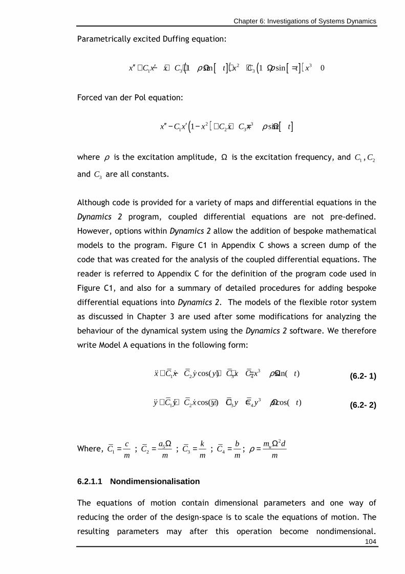
Chapter 6: Investigations of Systems Dynamics
104
Parametrically excited Duffing equation:
[ ]( ) [ ]( )2 31 3 31 sin 1 sin 0x C x x C t x C t xρ ρ′′ ′+ − + + Ω + + Ω =
Forced van der Pol equation:
( ) [ ]2 31 2 31 sinx C x x C x C x tρ′′ ′− − + + = Ω
where ρ is the excitation amplitude, Ω is the excitation frequency, and 1C , 2C
and 3C are all constants.
Although code is provided for a variety of maps and differential equations in the
Dynamics 2 program, coupled differential equations are not pre-defined.
However, options within Dynamics 2 allow the addition of bespoke mathematical
models to the program. Figure C1 in Appendix C shows a screen dump of the
code that was created for the analysis of the coupled differential equations. The
reader is referred to Appendix C for the definition of the program code used in
Figure C1, and also for a summary of detailed procedures for adding bespoke
differential equations into Dynamics 2. The models of the flexible rotor system
as discussed in Chapter 3 are used after some modifications for analyzing the
behaviour of the dynamical system using the Dynamics 2 software. We therefore
write Model A equations in the following form:
31 2 3 4cos( ) sin( )x C x C y y C x C x tρ+ − + + = Ωɺɺ ɺ ɺ (6.2- 1)
31 2 3 4cos( ) cos( )y C y C x y C y C y tρ+ + + + = Ωɺɺ ɺ ɺ (6.2- 2)
Where, 1
cC
m= ; 5
2
aC
m
Ω= ; 3
kC
m= ; 4
bC
m= ;
2um d
mρ Ω=
6.2.1.1 Nondimensionalisation
The equations of motion contain dimensional parameters and one way of
reducing the order of the design-space is to scale the equations of motion. The
resulting parameters may after this operation become nondimensional.
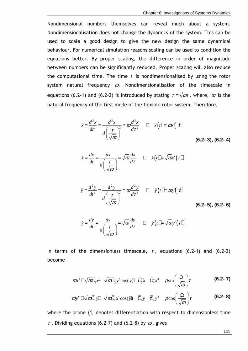
Chapter 6: Investigations of Systems Dynamics
105
Nondimensional numbers themselves can reveal much about a system.
Nondimensionalisation does not change the dynamics of the system. This can be
used to scale a good design to give the new design the same dynamical
behaviour. For numerical simulation reasons scaling can be used to condition the
equations better. By proper scaling, the difference in order of magnitude
between numbers can be significantly reduced. Proper scaling will also reduce
the computational time. The time t is nondimensionalised by using the rotor
system natural frequency ω . Nondimensionalisation of the timescale in
equations (6.2-1) and (6.2-2) is introduced by stating tτ ω= , where, ω is the
natural frequency of the first mode of the flexible rotor system. Therefore,
( ) ( )
2 2 2
22 2
d x d x d xx x t x
dt dd
ω ω τττ
ω
′′= = = ∴ =
ɺɺ ɺɺ
( ) ( )dx dx dxx x t x
dt dd
ω ω τττ
ω
′= = = ∴ =
ɺ ɺ
(6.2- 3), (6.2- 4)
( ) ( )
2 2 2
22 2
d y d y d yy y t y
dt dd
ω ω τττ
ω
′′= = = ∴ =
ɺɺ ɺɺ
( ) ( )dy dy dyy y t y
dt dd
ω ω τττ
ω
′= = = ∴ =
ɺ ɺ
(6.2- 5), (6.2- 6)
In terms of the dimensionless timescale, τ , equations (6.2-1) and (6.2-2)
become
3
1 2 3 4cos( ) sinx C x C y y C x C xω ω ω ρ τω
Ω ′′ ′ ′+ − + + =
(6.2- 7)
3
1 2 3 4cos( ) cosy C y C x y C y C yω ω ω ρ τω
Ω ′′ ′ ′+ + + + =
(6.2- 8)
where the prime ( )' denotes differentiation with respect to dimensionless time
τ . Dividing equations (6.2-7) and (6.2-8) by ω , gives
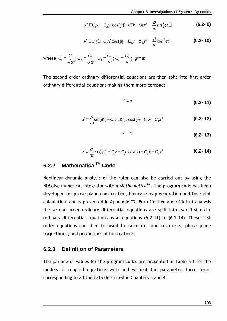
Chapter 6: Investigations of Systems Dynamics
106
( )31 2 3 4cos( ) sinx C x C y y C x C x t
ρ φω
′′ ′ ′+ − + + = (6.2- 9)
( )31 2 3 4cos( ) cosy C y C x y C y C y t
ρ φω
′′ ′ ′+ + + + = (6.2- 10)
where, 11
CC
ω= ; 2
2
CC
ω= ; 3
3
CC
ω= ; 4
4
CC
ω= ; φ ω=
The second order ordinary differential equations are then split into first order
ordinary differential equations making them more compact.
x u′ = (6.2- 11)
31 2 3 4sin( ) cos( )u t C u C v y C x C x
ρ φω
′ = − + − − (6.2- 12)
y v′ = (6.2- 13)
31 2 3 4cos( ) cos( )v t C v C u y C x C x
ρ φω
′ = − − − − (6.2- 14)
6.2.2 Mathematica TM Code
Nonlinear dynamic analysis of the rotor can also be carried out by using the
NDSolve numerical integrator within MathematicaTM. The program code has been
developed for phase plane construction, Poincaré map generation and time plot
calculation, and is presented in Appendix C2. For effective and efficient analysis
the second order ordinary differential equations are split into two first order
ordinary differential equations as at equations (6.2-11) to (6.2-14). These first
order equations can then be used to calculate time responses, phase plane
trajectories, and predictions of bifurcations.
6.2.3 Definition of Parameters
The parameter values for the program codes are presented in Table 6-1 for the
models of coupled equations with and without the parametric force term,
corresponding to all the data described in Chapters 3 and 4.
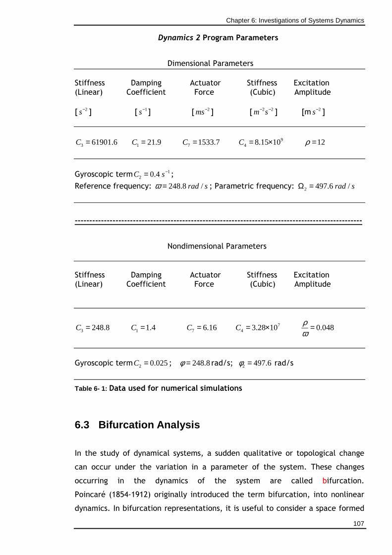
Chapter 6: Investigations of Systems Dynamics
107
Dynamics 2 Program Parameters
Dimensional Parameters Stiffness Damping Actuator Stiffness Excitation (Linear) Coefficient Force (Cubic) Amplitude [ 2s− ] [ 1s− ] [ 2ms− ] [ 2 2m s− − ] [m 2s− ]
3 61901.6C = 1 21.9C = 7 1533.7C = 94 8.15 10C = × 12ρ =
Gyroscopic term 1
2 0.4C s−= ;
Reference frequency: 248.8 /rad sω = ; Parametric frequency: 2 497.6 /rad sΩ =
---------------------------------------------------------------------------------------------------
Nondimensional Parameters Stiffness Damping Actuator Stiffness Excitation (Linear) Coefficient Force (Cubic) Amplitude
3 248.8C = 1 1.4C = 7 6.16C = 74 3.28 10C = × 0.048
ρω
=
Gyroscopic term 2 0.025C = ; 248.8φ = rad/s; 2 497.6φ = rad/s
Table 6- 1: Data used for numerical simulations
6.3 Bifurcation Analysis
In the study of dynamical systems, a sudden qualitative or topological change
can occur under the variation in a parameter of the system. These changes
occurring in the dynamics of the system are called bifurcation.
Poincaré (1854-1912) originally introduced the term bifurcation, into nonlinear
dynamics. In bifurcation representations, it is useful to consider a space formed
Chapter 6: Investigations of Systems Dynamics
108
by using the state variable(s) and chosen control parameter(s), called the state-
control space. Locations at which bifurcations occur in this space are called
bifurcation points. It is often desirable to know where in the parameter space
nonperiodic motion exists. Bifurcation diagrams can be used to indicate such
domains. A bifurcation diagram provides a summary of the essential dynamics of
systems and is therefore a useful way of observing nonlinear dynamic behaviour
(Chang-Jian et.al., 2007).
A periodic motion may become unstable if the control parameters are allowed to
vary, a scenario signifying dynamic deterioration of stability that could lead to
eventual chaos. In literature, there are various types of bifurcations, however,
in the present analysis a period doubling bifurcation can mostly be observed and
is analysed in the following sections in detail. It is a bifurcation in which the
system’s behaviour changes at integer multiples of the periodicity of the original
response. If the control parameter is further varied, the motion may become
chaotic. Appearance of multi-periodic motion indicates the set-in of dynamic
instability. Bifurcation helps in identifying instabilities in dynamical systems and
provides theoretical and practical ideas for controlling these systems and
optimizing their operation.
In understanding the dynamics within the models in Chapter 3, the Dynamics 2
software was used to plot the bifurcatory behaviour of the amplitude responses
as a function of normalised excitation acceleration and the Lyapunov exponent,
and these are illustrated in Figures 6-2 to 6-4. All data used for these plots are
system parameters taken from the experimental rig and graphs are plotted using
nondimensionalised parameters tabulated in Table 6-1. All the figures are
plotted using certain necessary Dynamics 2 commands and are summarised in
Table 6-2.
For a full understanding of these commands, the reader is referred to the
definitions of these commands in Appendix C and the text entitled “Numerical
Explorations” by Nusse and Yorke (1998).
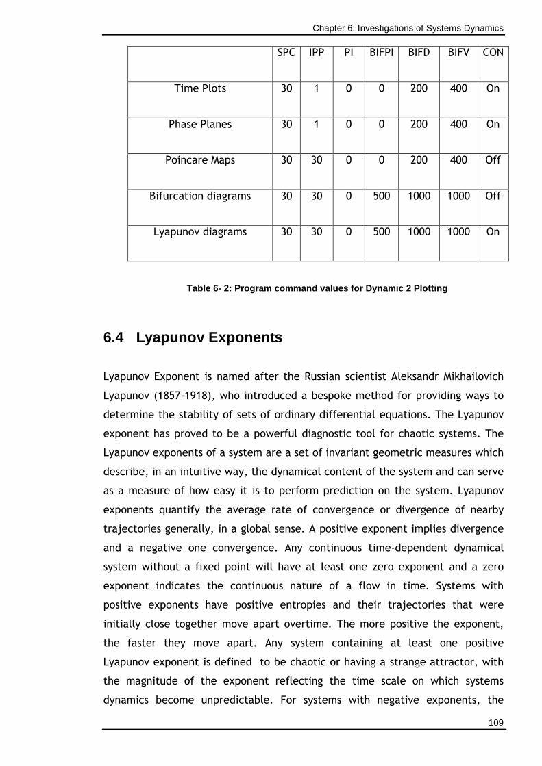
Chapter 6: Investigations of Systems Dynamics
109
SPC IPP PI BIFPI BIFD BIFV CON
Time Plots 30 1 0 0 200 400 On
Phase Planes 30 1 0 0 200 400 On
Poincare Maps 30 30 0 0 200 400 Off
Bifurcation diagrams 30 30 0 500 1000 1000 Off
Lyapunov diagrams 30 30 0 500 1000 1000 On
Table 6- 2: Progra m command values for Dynamic 2 Plotting
6.4 Lyapunov Exponents
Lyapunov Exponent is named after the Russian scientist Aleksandr Mikhailovich
Lyapunov (1857-1918), who introduced a bespoke method for providing ways to
determine the stability of sets of ordinary differential equations. The Lyapunov
exponent has proved to be a powerful diagnostic tool for chaotic systems. The
Lyapunov exponents of a system are a set of invariant geometric measures which
describe, in an intuitive way, the dynamical content of the system and can serve
as a measure of how easy it is to perform prediction on the system. Lyapunov
exponents quantify the average rate of convergence or divergence of nearby
trajectories generally, in a global sense. A positive exponent implies divergence
and a negative one convergence. Any continuous time-dependent dynamical
system without a fixed point will have at least one zero exponent and a zero
exponent indicates the continuous nature of a flow in time. Systems with
positive exponents have positive entropies and their trajectories that were
initially close together move apart overtime. The more positive the exponent,
the faster they move apart. Any system containing at least one positive
Lyapunov exponent is defined to be chaotic or having a strange attractor, with
the magnitude of the exponent reflecting the time scale on which systems
dynamics become unpredictable. For systems with negative exponents, the
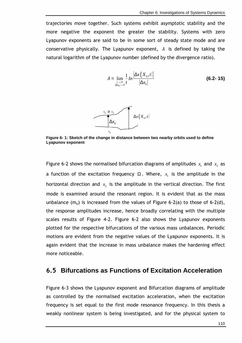
Chapter 6: Investigations of Systems Dynamics
110
trajectories move together. Such systems exhibit asymptotic stability and the
more negative the exponent the greater the stability. Systems with zero
Lyapunov exponents are said to be in some sort of steady state mode and are
conservative physically. The Lyapunov exponent, λ is defined by taking the
natural logarithm of the Lyapunov number (defined by the divergence ratio).
( )
0
0
00
,1limtx
x X tIn
t xλ
→∞∆ →
∆=
∆ (6.2- 15)
Figure 6- 1: Sketch of the change in distance betwe en two nearby orbits used to define Lyapunov exponent
Figure 6-2 shows the normalised bifurcation diagrams of amplitudes 1x and 2x as
a function of the excitation frequency Ω . Where, 1x is the amplitude in the
horizontal direction and 2x is the amplitude in the vertical direction. The first
mode is examined around the resonant region. It is evident that as the mass
unbalance (mu) is increased from the values of Figure 6-2(a) to those of 6-2(d),
the response amplitudes increase, hence broadly correlating with the multiple
scales results of Figure 4-2. Figure 6-2 also shows the Lyapunov exponents
plotted for the respective bifurcations of the various mass unbalances. Periodic
motions are evident from the negative values of the Lyapunov exponents. It is
again evident that the increase in mass unbalance makes the hardening effect
more noticeable.
6.5 Bifurcations as Functions of Excitation Accelerati on
Figure 6-3 shows the Lyapunov exponent and Bifurcation diagrams of amplitude
as controlled by the normalised excitation acceleration, when the excitation
frequency is set equal to the first mode resonance frequency. In this thesis a
weakly nonlinear system is being investigated, and for the physical system to
0 0x x+ ∆
0x
( )0,x X t∆ 0x∆
Chapter 6: Investigations of Systems Dynamics
111
become more intrinsically nonlinear the excitation acceleration and the
nonlinear cubic coefficient values have to be increased either by increasing the
mass unbalance or by making the shaft more flexible, or both. Therefore in
order to obtain and investigate the situation when the system is more strongly
nonlinear the mass unbalance value is artificially increased to various multiples
of the actual value. This manipulation increases the excitation value to a high
level driving the weakly nonlinear system into more nonlinear reaches of the
response range making the effect of the nonlinear terms proportionally greater
than they would otherwise be. This effect causes the system to show possible
bifurcations to chaos. The periodic response for the case based on the smallest
mass unbalance in Figure 6-3(a) (i.e. the most weakly nonlinear response in
Chapters 4 to 6), bifurcates to chaos as the mass unbalance increases. Positive
Lyapunov exponents for figures 6-3(a)-(d) respectively show clear indication of
chaos, while the negative Lyapunov exponents show stable motion. Also from
these graphs, as the response become chaotic, less excitation acceleration is
required in each of the four cases successively. One finds that five kinds of
system motion exits over the range of excitation acceleration values. These are
stable single period motion, stable period two motion, stable period four
motion, stable quasi-periodic or multiperiod motion, and chaotic motion.
Figure 6-3(a) shows the bifurcation in the horizontal direction as controlled by
the normalised excitation acceleration at a mass unbalance of 0.004um kg= ,
using the first mode resonance frequency value Ω from Table 6-1. It appears
that for normalised excitation acceleration values from 200 to 730, the iterates
settle down onto a fixed point. This is considered to be period one motion. At
the value of 730 the fixed point becomes unstable and the period doubles, i.e.
the iterates visit two different values in turn. At this value the period one
motion becomes unstable in favour of a stable period two motion. Figure 6-3(b)
and (c) show the bifurcation in the horizontal direction as controlled by
excitation acceleration for the mass unbalance values 3 um and 4 um respectively.
By increasing the mass unbalance values the periodic response bifurcates to
period doubling and finally to chaos. Negative Lyapunov exponents show stable
motion, while the positive Lyapunov exponents show clear indication of chaos.
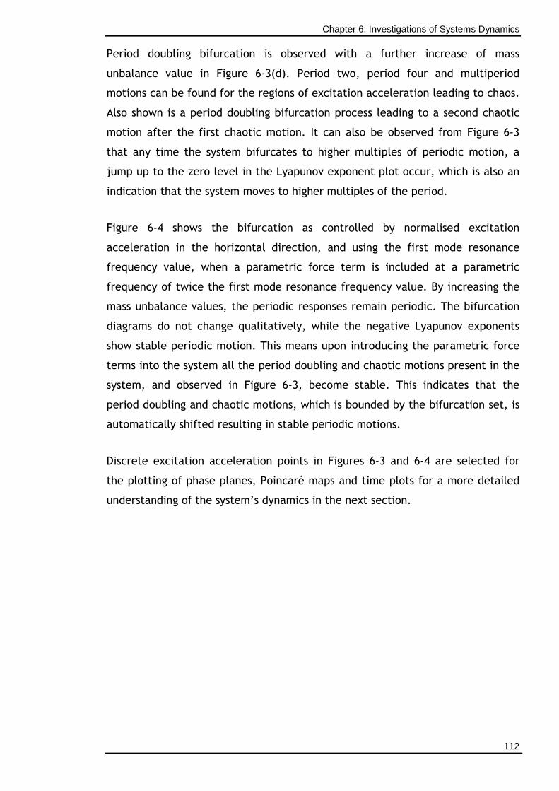
Chapter 6: Investigations of Systems Dynamics
112
Period doubling bifurcation is observed with a further increase of mass
unbalance value in Figure 6-3(d). Period two, period four and multiperiod
motions can be found for the regions of excitation acceleration leading to chaos.
Also shown is a period doubling bifurcation process leading to a second chaotic
motion after the first chaotic motion. It can also be observed from Figure 6-3
that any time the system bifurcates to higher multiples of periodic motion, a
jump up to the zero level in the Lyapunov exponent plot occur, which is also an
indication that the system moves to higher multiples of the period.
Figure 6-4 shows the bifurcation as controlled by normalised excitation
acceleration in the horizontal direction, and using the first mode resonance
frequency value, when a parametric force term is included at a parametric
frequency of twice the first mode resonance frequency value. By increasing the
mass unbalance values, the periodic responses remain periodic. The bifurcation
diagrams do not change qualitatively, while the negative Lyapunov exponents
show stable periodic motion. This means upon introducing the parametric force
terms into the system all the period doubling and chaotic motions present in the
system, and observed in Figure 6-3, become stable. This indicates that the
period doubling and chaotic motions, which is bounded by the bifurcation set, is
automatically shifted resulting in stable periodic motions.
Discrete excitation acceleration points in Figures 6-3 and 6-4 are selected for
the plotting of phase planes, Poincaré maps and time plots for a more detailed
understanding of the system’s dynamics in the next section.
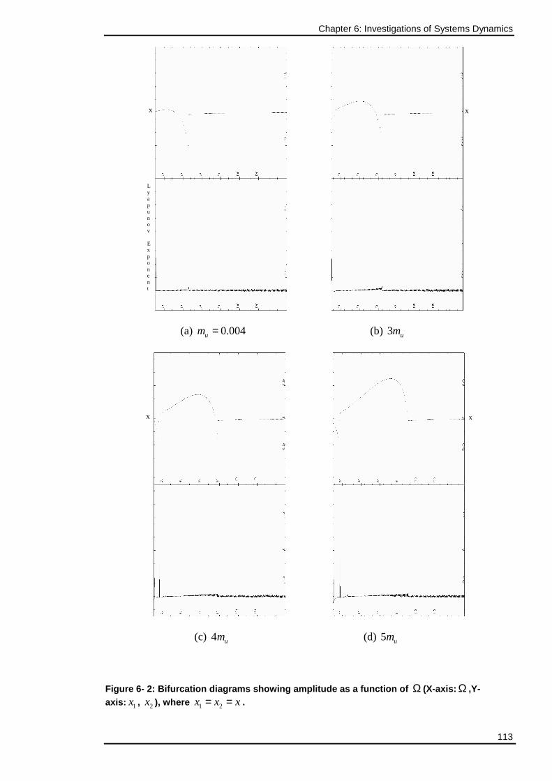
Chapter 6: Investigations of Systems Dynamics
113
(a) 0.004um = (b) 3 um
(c) 4 um (d) 5 um
Figure 6- 2: Bifurcation diagrams showing amplitude as a function of Ω (X-axis: Ω ,Y-axis: 1x , 2x ), where 1 2x x x= = .
L y a p u n o v E x p o n e n t
x x
x x
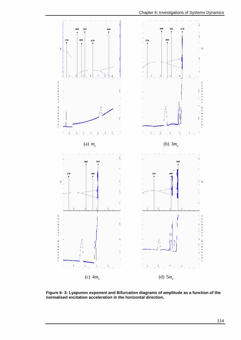
Chapter 6: Investigations of Systems Dynamics
114
(a) um (b) 3 um
(c) 4 um (d) 5 um
Figure 6- 3: Lyapunov exponent and Bifurcation diag rams of amplitude as a function of the normalised excitation acceleration in the horizonta l direction.
L y a p u n o v E x p o n e n t
L y a p u n o v E x p o n e n t
L y a p u n o v E x p o n e n t
L y a p u n o v E x p o n e n t
x
x x
x
250
400
460
505
250 618
840 400
460
505 618
250
400
460
505
250 400
460
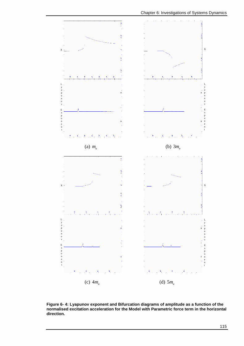
Chapter 6: Investigations of Systems Dynamics
115
(a) um (b) 3 um
(c) 4 um (d) 5 um
Figure 6- 4: Lyapunov exponent and Bifurcation diag rams of amplitude as a function of the normalised excitation acceleration for the Model wi th Parametric force term in the horizontal direction.
L y a p u n o v
E x p o n e n t
L y a p u n o v E x p o n e n t
L y a p u n o v E x p o n e n t
L y a p u n o v
E x p o n e n t
x
x x
x
Chapter 6: Investigations of Systems Dynamics
116
6.6 Phase Planes, Poincaré Maps and Time Plots
The response of a dynamic system in general could be a fixed point, a periodic
solution, or a non-periodic solution. By studying the geometric characteristics
and flow paths of the solution trajectory in the state space, the stability near
the trajectory can be determined using phase portraits. For a trajectory that
follows a close orbit in the phase portrait and returns precisely to where it first
started after a period T, the motion is periodic and the closed orbit is called a
limit cycle. Chaotic motions, on the other hand, have orbits that never close or
repeat. Thus, the trajectory of the orbits in the phase plane will tend to fill up a
section of the phase space. Although wandering of orbits is a clue to chaos,
continuous phase plots provide very little information and one must use a
modified phase plane technique called Poincaré mapping.
Poincaré map is a qualitative topological approach widely applied to the
predictions of chaos and the study of stability in the phase space through
exploring the geometric features of the sequence of points on a Poincaré
section. A Poincaré section is a hypersurface in the state phase transverse to the
flow of a system. In non-autonomous systems, points on the Poincaré sections
represent the return points of the time series at a constant interval T, where T
is the driving period of the existing force. The projection of all points in a
Poincaré section to their image points by following trajectories until they first
return to the Poincaré section is referred to as Poincaré map of the dynamic
system. For a periodically forced, second-order nonlinear oscillator, a Poincaré
map can be obtained by stroboscopically observing the position and velocity at a
particular phase of the forcing functions. For quasi-periodic motion, the returns
points in the Poincaré map form a closed curve. For a system undergoing chaotic
motion, its associated Poincaré map shows specific shapes or many irregular
points and features indicating the state and extent of bifurcation. For nT-
periodic motion, the return points in the Poincaré map are n discrete points.
Chapter 6: Investigations of Systems Dynamics
117
6.6.1 Analysis of Phase Planes, Poincaré Maps and T ime Plots
More detailed analysis of Figures 6-3 and 6-4 are extended to phase planes,
Poincaré maps and time plots (i.e. Figures 6-5 to 6-11) at discrete excitation
acceleration points. The phase plane and time plots are plotted at assumed
steady-state conditions, taken to be during the interval t=995-1000 seconds.
However, the Poincaré maps are plotted from the transient time (i.e. t=0 to
1000 seconds) as most of them converge to a period one motion with just a
point, therefore richer diagrams are preferred and so these maps converge to
darker areas and finally to a point attractor. Those that are not in period one
motion show irregular structures, or strange attractors, or a number of irregular
points. A break-down of the observations for the sets of coupled equations with
and without parametric terms is as follows.
6.6.1.1 At Normalised Excitation Acceleration of 25 0 (Figure 6-5):
• All the bifurcation diagrams for the different values of mass unbalance
show periodic and stable motions with negative Lyapunov exponents as
depicted in Figures 6-3 (a) to (d).
• The phase planes show a single closed orbit, showing only stationary,
post-transient motion. The orbit is single and periodic, corresponding with
the bifurcation diagrams. It indicates a period one motion. The solutions
show regular patterns in the steady-state region of time t=995-1000
seconds and are indicative of stable periodic solutions.
• All the Poincaré maps converge into a single point (circled). As the maps
consist of one point, which implies periodic motion, it indicates a period
one motion with a stable attractor.
• All the time plots show evidence of a periodic response.
Chapter 6: Investigations of Systems Dynamics
118
6.6.1.2 At Normalised Excitation Acceleration of 40 0 (Figure 6-6):
• The bifurcation diagrams in Figure 6-3(a) and (b) show period one motion
whereas Figure 6-3 (c) and (d) show period two and period four motions,
respectively. All the motions are stable, with negative Lyapunov
exponents.
• Their corresponding phase planes indicate the period doubling
phenomena. Figures 6-6(a) and (b) show single closed orbits indicating a
period one motion and 6-6(c) show a closed orbit crossing itself, and
depicts a period two motion as in their bifurcation diagrams. Figure 6-6(d)
show a period four motion as in their bifurcation diagrams. The orbits
show regular pattern indicating stable solutions.
• The Poincaré maps consist of a finite number of points, implying periodic
motions. In Figures 6-6(a),(b),(c) and (d), the maps converge to one, two
and four distinct points indicating stable period one, period two and
period four motions, respectively.
• All the time plots show evidence of periodic motions.
6.6.1.3 At Normalised Excitation Acceleration of 46 0 (Figure 6-7):
• The bifurcation diagrams for 5 um , in Figure 6-3(d), show chaotic motion
with positive Lyapunov exponents, whereas that for 4 um , in Figure 6-3(c)
shows period two motion with a negative Lyapunov exponent. All the
others are in period one motion.
• The phase planes underpin the above. For the chaotic motions densely
filled phase planes are obtained. The plots have overlaid, complicated
and repeated orbit cross-overs. Had the simulation been allowed to
continue, the plane would be even more overlaid by repeated orbit cross-
overs. A complicated phase plot is one indicator of chaotic motion;
however, motion that rides on a complicated looking orbit may very well
be fully-predictable, and thus non-chaotic, because a phase plot with very
Chapter 6: Investigations of Systems Dynamics
119
large numbers of degrees-of-freedom may look similarly complicated,
even if the system is in fact linear and thus certainly non-chaotic.
• In Figures 6-7(a) and (b) the Poincaré maps show one distinct point
indicating stable period one motion, and in Figures 6-7(c), 2 distinct
points are shown indicating stable period two motion, whereas in Figures
6-7(d) the Poincaré map shows irregular shape and is that of chaotic
motion, where more and more points are added to the map as the
simulation time marches on, filling out the details of the strange attractor
on which the chaotic motion rides, and therefore indicative of chaotic
motion.
• The time plots are in periodic motion, except for one in Figure 6-7(d)
where the oscillations never repeat. This is another qualitative visual
indicator of chaotic motions.
6.6.1.4 At Normalised Excitation Acceleration of 50 5 (Figure 6-8):
• Bifurcation diagrams in Figures 6-3(a) and (b) show period one and period
two motions respectively with negative Lyapunov exponents, whereas
Figure 6-3(c) show chaotic motions with positive Lyapunov exponents.
• The phase planes underpin the above. For the chaotic motions densely
filled phase planes are obtained. The plots have overlaid, complicated
and repeated orbit cross-overs. Figures 6-8(a) and (b) show closed orbits
indicating period one and period two motions respectively.
• In Figures 6-8(a) and (b) the Poincaré maps show one and two distinct
points respectively indicating stable period one and period two motions
respectively, and in Figures 6-8(c) the Poincaré map shows an irregular
shape and is that of chaotic motion.
• The time plots in Figures 6-8(a) and (b) show stable motions, but the plot
in Figure 6-8(c) is non-periodic, the oscillations do not repeat, indicating
chaotic motion.
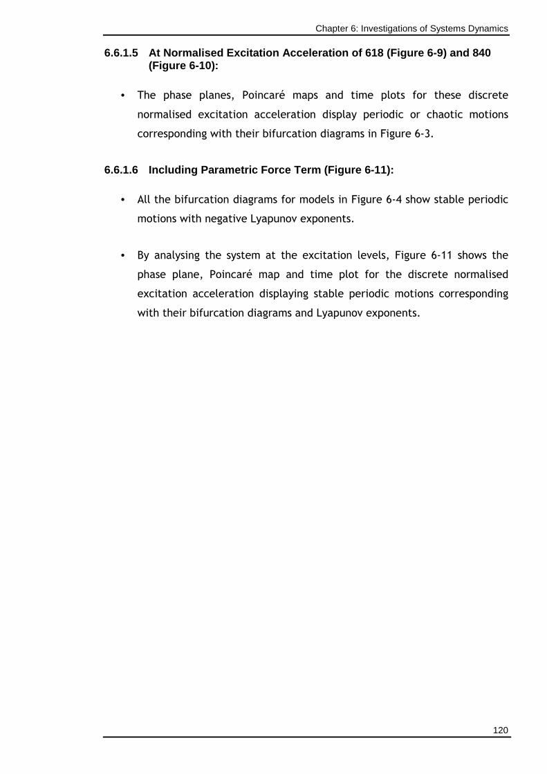
Chapter 6: Investigations of Systems Dynamics
120
6.6.1.5 At Normalised Excitation Acceleration of 61 8 (Figure 6-9) and 840 (Figure 6-10):
• The phase planes, Poincaré maps and time plots for these discrete
normalised excitation acceleration display periodic or chaotic motions
corresponding with their bifurcation diagrams in Figure 6-3.
6.6.1.6 Including Parametric Force Term (Figure 6-1 1):
• All the bifurcation diagrams for models in Figure 6-4 show stable periodic
motions with negative Lyapunov exponents.
• By analysing the system at the excitation levels, Figure 6-11 shows the
phase plane, Poincaré map and time plot for the discrete normalised
excitation acceleration displaying stable periodic motions corresponding
with their bifurcation diagrams and Lyapunov exponents.
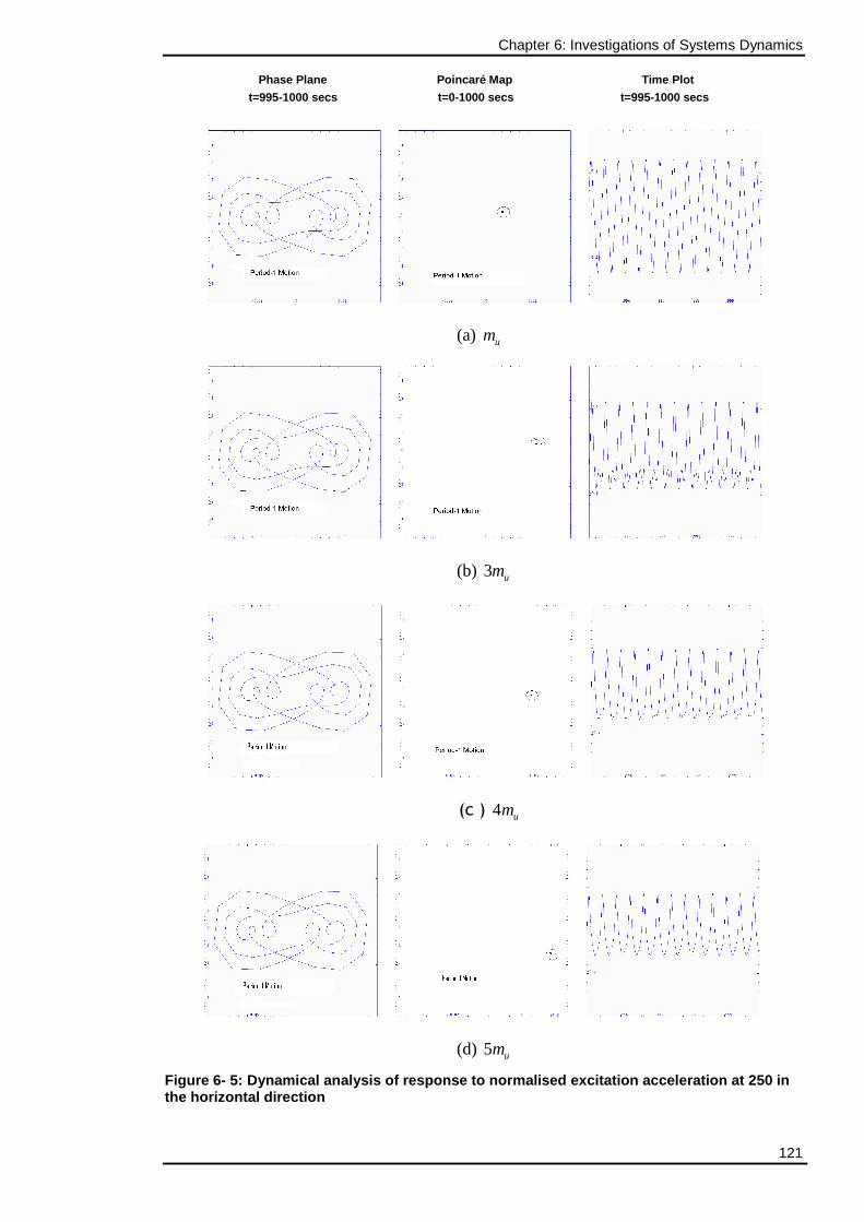
Chapter 6: Investigations of Systems Dynamics
121
Phase Plane Poincaré Map Time Plot
t=995-1000 secs t=0-1 000 secs t=995-1000 secs
(a) um
(b) 3 um
(c ) 4 um
(d) 5 um
Figure 6- 5: Dynamical analysis of response to norm alised excitation acceleration at 250 in the horizontal direction
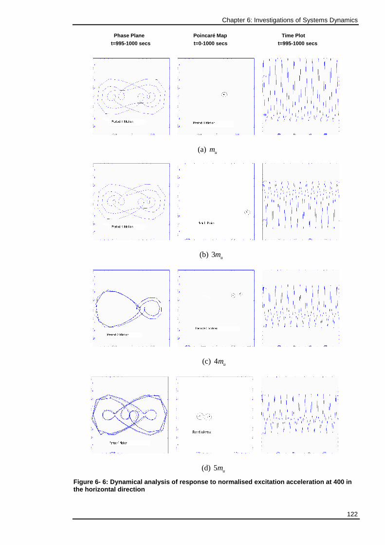
Chapter 6: Investigations of Systems Dynamics
122
Phase Plane Poinca ré Map Time Pl ot
t=995-1000 secs t=0-1000 secs t=995-1000 secs
(a) um
(b) 3 um
(c) 4 um
(d) 5 um
Figure 6- 6: Dynamical analysis of response to norm alised excitation acceleration at 400 in the horizontal direction
Chapter 6: Investigations of Systems Dynamics
123
Phase Plane Poi ncaré Map T ime Plot
t=995-1000 secs t=0 -1000 secs t=9 95-1000 secs
(a) um
(b) 3 um
(c) 4 um
(d) 5 um
Figure 6- 7: Dynamical analysis of response to norm alised excitation acceleration at 460 in the horizontal direction
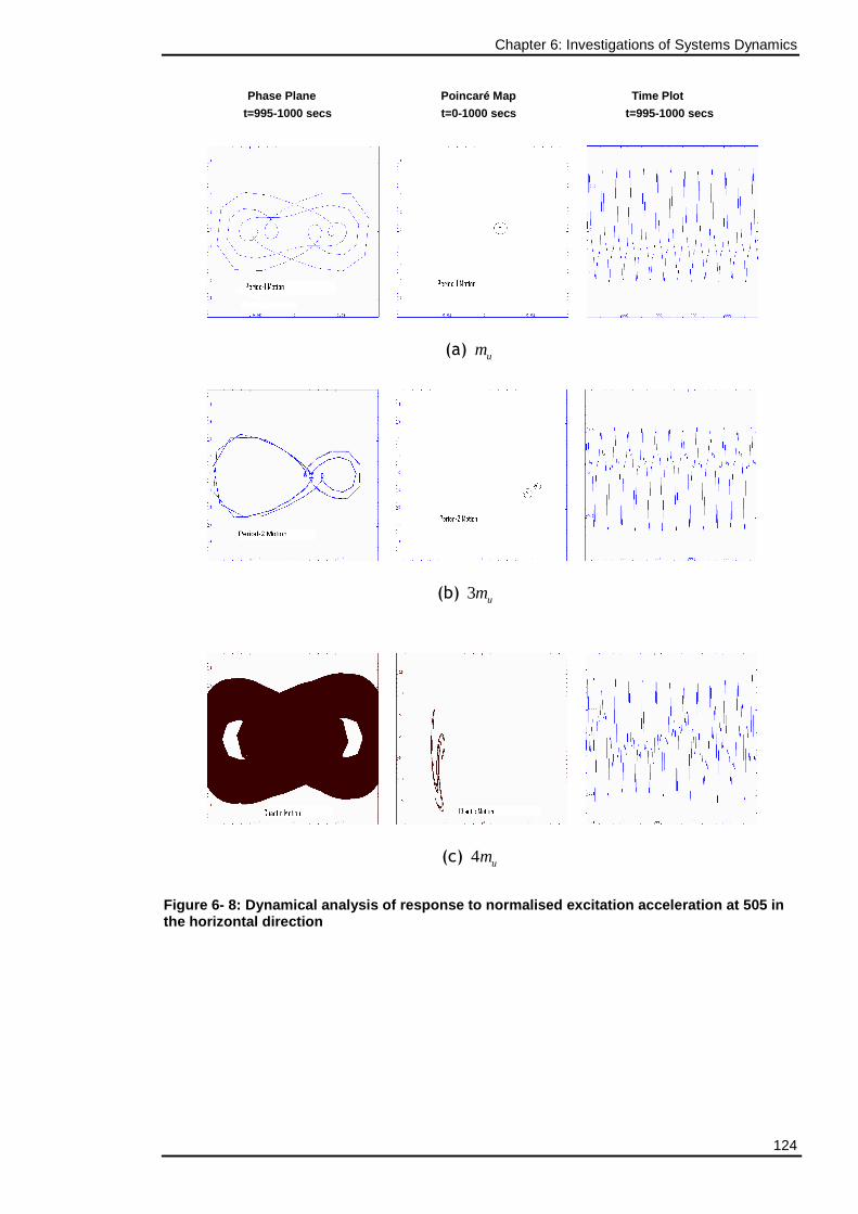
Chapter 6: Investigations of Systems Dynamics
124
Phase Plane P oincaré Map Time Plot
t=995-1000 secs t= 0-1000 secs t=995- 1000 secs
(a) um
(b) 3 um
(c) 4 um
Figure 6- 8: Dynamical analysis of response to norm alised excitation acceleration at 505 in the horizontal direction
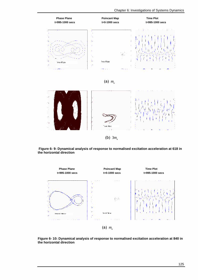
Chapter 6: Investigations of Systems Dynamics
125
Phase Plane Poincaré Map Ti me Plot
t=995-1000 secs t=0-1000 secs t= 995-1000 secs
(a) um
(b) 3 um
Figure 6- 9: Dynamical analysis of response to nor malised excitation acceleration at 618 in the horizontal direction
Phase Plane P oincaré Map Time Pl ot
t=995-1000 secs t=0-1000 secs t=995-1000 secs
(a) um
Figure 6- 10: Dynamical analysis of response to nor malised excitation acceleration at 840 in the horizontal direction
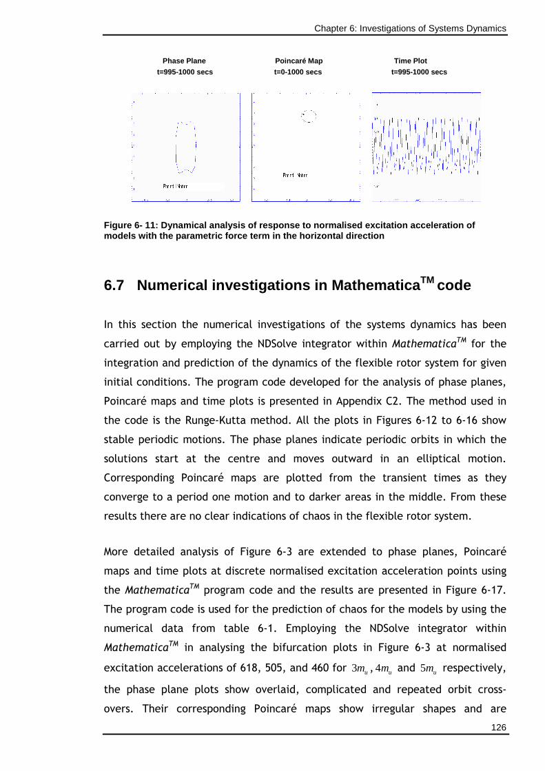
Chapter 6: Investigations of Systems Dynamics
126
Phase Plane Poinca ré Map Time Plot
t=995-1000 secs t=0-1000 secs t=995-1000 secs
Figure 6- 11: Dynamical analysis of response to nor malised excitation acceleration of models with the parametric force term in the horizo ntal direction
6.7 Numerical investigations in MathematicaTM code
In this section the numerical investigations of the systems dynamics has been
carried out by employing the NDSolve integrator within MathematicaTM for the
integration and prediction of the dynamics of the flexible rotor system for given
initial conditions. The program code developed for the analysis of phase planes,
Poincaré maps and time plots is presented in Appendix C2. The method used in
the code is the Runge-Kutta method. All the plots in Figures 6-12 to 6-16 show
stable periodic motions. The phase planes indicate periodic orbits in which the
solutions start at the centre and moves outward in an elliptical motion.
Corresponding Poincaré maps are plotted from the transient times as they
converge to a period one motion and to darker areas in the middle. From these
results there are no clear indications of chaos in the flexible rotor system.
More detailed analysis of Figure 6-3 are extended to phase planes, Poincaré
maps and time plots at discrete normalised excitation acceleration points using
the MathematicaTM program code and the results are presented in Figure 6-17.
The program code is used for the prediction of chaos for the models by using the
numerical data from table 6-1. Employing the NDSolve integrator within
MathematicaTM in analysing the bifurcation plots in Figure 6-3 at normalised
excitation accelerations of 618, 505, and 460 for 3 um ,4 um and 5 um respectively,
the phase plane plots show overlaid, complicated and repeated orbit cross-
overs. Their corresponding Poincaré maps show irregular shapes and are
Chapter 6: Investigations of Systems Dynamics
127
indicative of chaotic motion. The time plots are non-periodic, the oscillations do
not repeat and all the results mirror those in Figures 6-7(d) and 6-8 (c) and 6-9
(b) respectively.
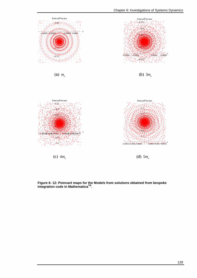
Chapter 6: Investigations of Systems Dynamics
128
-0.0001-0.00005 0.000050.0001x
-0.13
-0.12
-0.11
-0.09
x'Poincare Section
-0.0004 -0.0002 0.0002 0.0004x
-0.525
-0.475
-0.45
-0.425
-0.4
-0.375
x'Poincare Section
(a) um (b) 3 um
-0.00075-0.0005-0.00025 0.000250.00050.00075x
-1.1
-1.05
-0.95
-0.9
-0.85
-0.8
-0.75
x'Poincare Section
-0.0015-0.001-0.0005 0.00050.0010.0015x
-1.7
-1.6
-1.5
-1.4
-1.3
-1.2
x'Poincare Section
(c) 4 um (d) 5 um
Figure 6- 12: Poincaré maps for the Models from sol utions obtained from bespoke integration code in MathematicaTM.

Chapter 6: Investigations of Systems Dynamics
129
Phase Plane Time Plot
-0.0015 -0.001 -0.0005 0 0.0005 0.001 0.0015x@tD
-0.3
-0.2
-0.1
0
0.1
0.2
0.3
x′ @tD
0 0.1 0.2 0.3 0.4 0.5
Time @sD
-0.0015
-0.001
-0.0005
0
0.0005
0.001
0.0015
x@tD
t= (0-0.5) seconds
-0.0015 -0.001 -0.0005 0 0.0005 0.001 0.0015x@tD
-0.3
-0.2
-0.1
0
0.1
0.2
0.3
x′ @tD
0 0.2 0.4 0.6 0.8 1
Time @sD
-0.0015
-0.001
-0.0005
0
0.0005
0.001
0.0015
x@tD
t= (0-1) seconds
-0.0015 -0.001 -0.0005 0 0.0005 0.001 0.0015x@tD
-0.3
-0.2
-0.1
0
0.1
0.2
0.3
x′ @tD
0 2 4 6 8 10
Time @sD
-0.0015
-0.001
-0.0005
0
0.0005
0.001
0.0015
x@tD
t= (0-10) seconds
-0.0015 -0.001 -0.0005 0 0.0005 0.001 0.0015x@tD
-0.3
-0.2
-0.1
0
0.1
0.2
0.3
x′ @tD
0 10 20 30 40 50
Time @sD
-0.0015
-0.001
-0.0005
0
0.0005
0.001
0.0015
x@tD
t= (0-50) seconds
Figure 6- 13: Phase planes and Time plots for m u from solutions obtained from bespoke integration code in MathematicaTM.
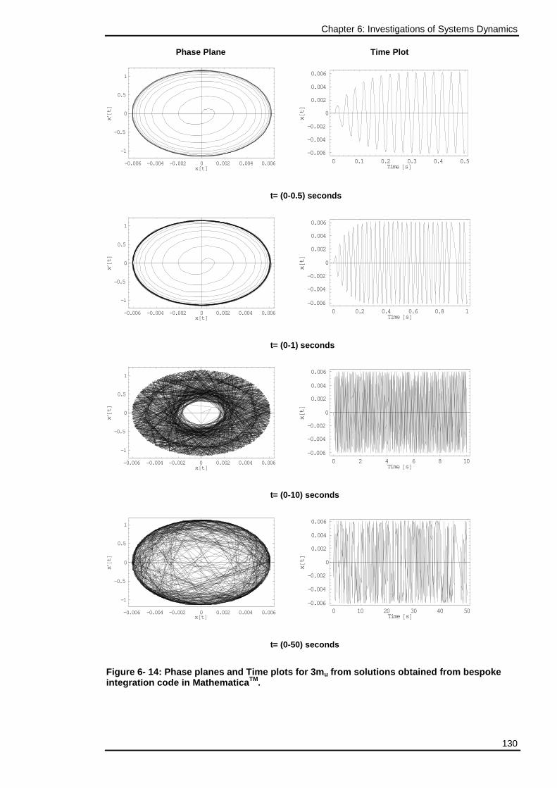
Chapter 6: Investigations of Systems Dynamics
130
Phase Plane Time Plot
-0.006 -0.004 -0.002 0 0.002 0.004 0.006x@tD
-1
-0.5
0
0.5
1
x′ @tD
0 0.1 0.2 0.3 0.4 0.5
Time @sD
-0.006
-0.004
-0.002
0
0.002
0.004
0.006
x@tD
t= (0-0.5) seconds
-0.006 -0.004 -0.002 0 0.002 0.004 0.006x@tD
-1
-0.5
0
0.5
1
x′ @tD
0 0.2 0.4 0.6 0.8 1
Time @sD
-0.006
-0.004
-0.002
0
0.002
0.004
0.006
x@tD
t= (0-1) seconds
-0.006 -0.004 -0.002 0 0.002 0.004 0.006x@tD
-1
-0.5
0
0.5
1
x′ @tD
0 2 4 6 8 10
Time @sD
-0.006
-0.004
-0.002
0
0.002
0.004
0.006
x@tD
t= (0-10) seconds
-0.006 -0.004 -0.002 0 0.002 0.004 0.006x@tD
-1
-0.5
0
0.5
1
x′@t
D
0 10 20 30 40 50
Time @sD
-0.006
-0.004
-0.002
0
0.002
0.004
0.006
x@tD
t= (0-50) seconds
Figure 6- 14: Phase planes and Time plots for 3m u from solutions obtained from bespoke integration code in MathematicaTM.
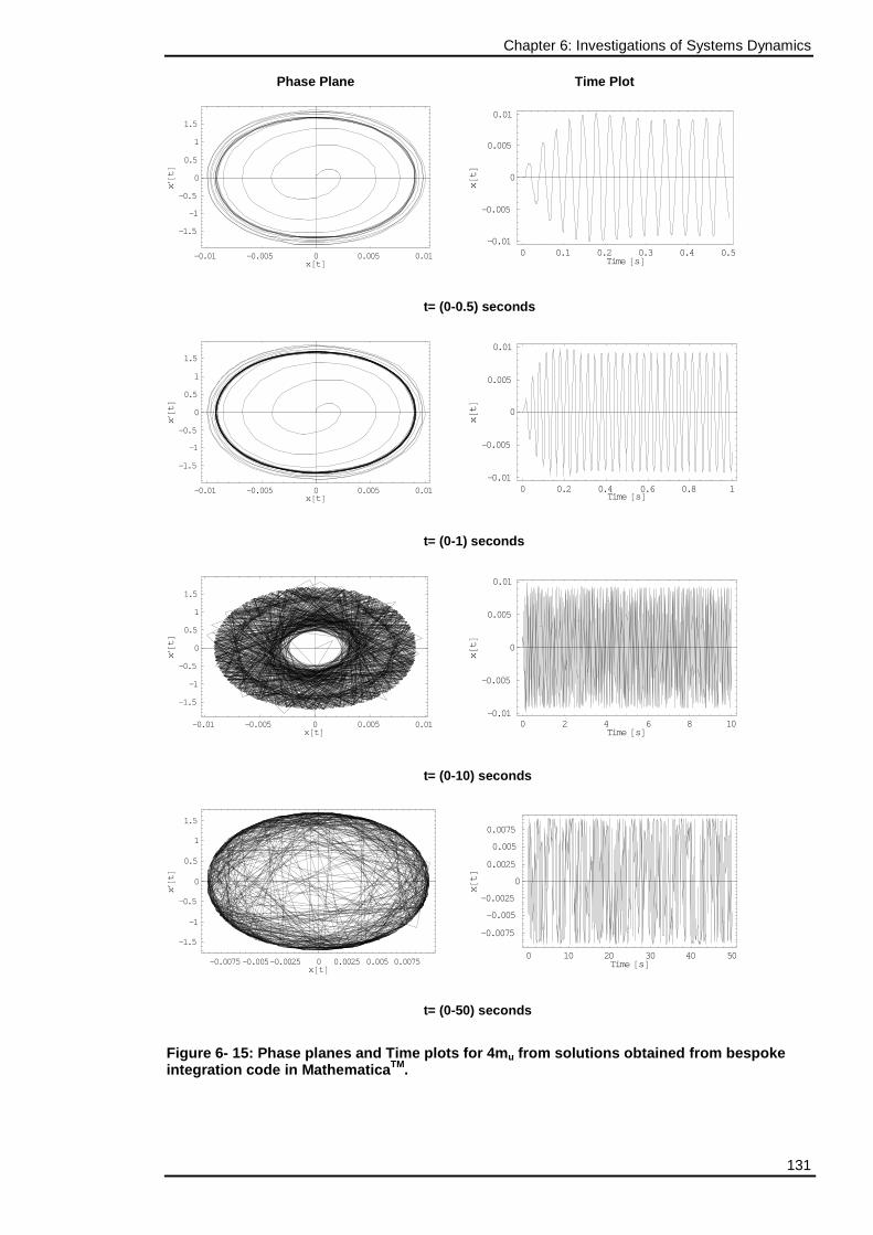
Chapter 6: Investigations of Systems Dynamics
131
Phase Plane Time Plot
-0.01 -0.005 0 0.005 0.01x@tD
-1.5
-1
-0.5
0
0.5
1
1.5
x′ @tD
0 0.1 0.2 0.3 0.4 0.5
Time @sD
-0.01
-0.005
0
0.005
0.01
x@tD
t= (0-0.5) seconds
-0.01 -0.005 0 0.005 0.01x@tD
-1.5
-1
-0.5
0
0.5
1
1.5
x′ @tD
0 0.2 0.4 0.6 0.8 1
Time @sD
-0.01
-0.005
0
0.005
0.01
x@tD
t= (0-1) seconds
-0.01 -0.005 0 0.005 0.01x@tD
-1.5
-1
-0.5
0
0.5
1
1.5
x′ @tD
0 2 4 6 8 10
Time @sD
-0.01
-0.005
0
0.005
0.01
x@tD
t= (0-10) seconds
-0.0075-0.005-0.0025 0 0.0025 0.005 0.0075x@tD
-1.5
-1
-0.5
0
0.5
1
1.5
x′@t
D
0 10 20 30 40 50
Time @sD
-0.0075
-0.005
-0.0025
0
0.0025
0.005
0.0075
x@tD
t= (0-50) seconds
Figure 6- 15: Phase planes and Time plots for 4m u from solutions obtained from bespoke integration code in MathematicaTM.
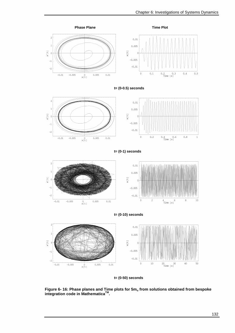
Chapter 6: Investigations of Systems Dynamics
132
Phase Plane Time Plot
-0.01 -0.005 0 0.005 0.01x@tD
-2
-1
0
1
2
x′ @tD
0 0.1 0.2 0.3 0.4 0.5
Time @sD
-0.01
-0.005
0
0.005
0.01
x@tD
t= (0-0.5) seconds
-0.01 -0.005 0 0.005 0.01x@tD
-2
-1
0
1
2
x′ @tD
0 0.2 0.4 0.6 0.8 1
Time @sD
-0.01
-0.005
0
0.005
0.01
x@tD
t= (0-1) seconds
-0.01 -0.005 0 0.005 0.01x@tD
-2
-1
0
1
2
x′ @tD
0 2 4 6 8 10
Time @sD
-0.01
-0.005
0
0.005
0.01
x@tD
t= (0-10) seconds
-0.01 -0.005 0 0.005 0.01x@tD
-2
-1
0
1
2
x′ @tD
0 10 20 30 40 50
Time @sD
-0.01
-0.005
0
0.005
0.01
x@tD
t= (0-50) seconds
Figure 6- 16: Phase planes and Time plots for 5m u from solutions obtained from bespoke integration code in MathematicaTM.
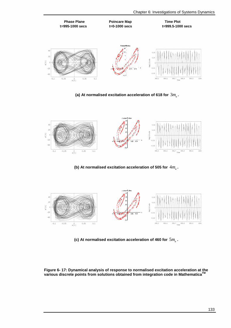
Chapter 6: Investigations of Systems Dynamics
133
Phase Plane Poincare Map Time Plot t=995-1000 secs t=0-1000 secs t=999.5-1000 secs
-0.1 -0.05 0 0.05 0.1x@tD
-40
-20
0
20
40
x′@t
D
999.5 999.6 999.7 999.8 999.9 1000
Time
-0.02
-0.01
0
0.01
0.02
edutil
pmA
(a) At normalised excitation acceleration of 618 fo r 3 um .
-0.1 -0.05 0 0.05 0.1x@tD
-40
-20
0
20
40
x′@t
D
999.5 999.6 999.7 999.8 999.9 1000
Time
-0.02
-0.01
0
0.01
0.02
edutil
pmA
(b) At normalised excitation acceleration of 505 fo r 4 um .
-0.1 -0.05 0 0.05 0.1x@tD
-40
-20
0
20
40
x′@t
D
999.5 999.6 999.7 999.8 999.9 1000
Time
-0.02
-0.01
0
0.01
0.02
edutil
pmA
(c) At normalised excitation acceleration of 460 fo r 5 um .
Figure 6- 17: Dynamical analysis of response to nor malised excitation acceleration at the various discrete points from solutions obtained fro m integration code in MathematicaTM
Chapter 7: Experimental Investigations
134
CHAPTER 7
EXPERIMENTAL INVESTIGATIONS
_________________________________________________
7.1 Controlling Flexible Rotor Vibration by means o f an
Antagonistic SMA/Composite Smart Bearing.
7.1.1 Introduction
The main themes of the research discussed in this chapter are the analysis and
the testing of systems of integrated structural components and active actuators.
In particular, systems are investigated comprising strategically designed and
applied SMA and piezoelectric elements, i.e. SMA strips within glass/epoxy
composites and piezoelectric stack actuators. Extensive recent research by śak
et.al., (2003) and Inman et.al., 2006 on the application of shape memory alloy
(SMA) elements integrated within glass epoxy composite plates and shells has led
to the design of a novel smart bearing based on the principle of antagonistic
action. In a previous work by śak et.al., (2003), a sleeve ring composite host
housing designed showed that a single SMA/composite active bearing could be
very effective at both altering the natural frequency of the fundamental whirl
mode as well as modifying the modal amplitude. The drawback of the single
ended SMA/composite active bearing design is the disparity in the time constant
between the relatively fast heating phase and the much slower cooling phase
which is entirely reliant on externally supplied forced air cooling. This is
principally because SMA can do no work when it is relaxing to its low
temperature state, and so this was a significant limitation for the work as
reported in the work of śak et.al., (2003). This has led to the antagonistic
design in this thesis, in which each half of the new bearing has its separate
heating as well as its own independent forced-air cooling system. The
antagonistic design results in virtually equalising the time constants and giving
faster responding push-pull loads on the centrally located bearing. This has the
consequent knock-on effect of making the system generally more conducive to
the control of resonant vibration.
Chapter 7: Experimental Investigations
135
It can often be useful to modify the frequencies of a rotor-shaft system. The
main motivation in such cases is to avoid critical speeds whilst running up and
running down rotors. The technique to be developed here is to use
SMA/composite technology within bearing housings in rotating machinery in
order to achieve optimal run-up and run-down of the rotor so that the effects of
all significant resonances are modified. There are a number of ways in which
variable pedestal properties may be devised to control the vibration levels and
rotor stresses in a rotating machine. One option is to vary pedestal and/or
bearing properties in such a way as to minimise the time a rotor spends at, or
near, a critical speed. During operation, vibration levels may be substantially
reduced by appropriate changes to support stiffness, causing changes to critical
speeds.
The solution proposed here is to use the SMA effect to control the stiffness of a
rotor bearing housing and hence manipulate the frequencies of the rotor system.
The work proposed is an outgrowth of the previous work of śak et.al., (2003)
and Segalman et. al., (1993) to use an SMA composite to actively change the
stiffness of the rotor system. This concept, attempted numerically in Segalman
et.al, (1993) with basic models, is to avoid critical speeds during run up and was
addressed by śak et.al., (2003) with improved modelling and experimental
implementation. śak et. al., (2003), showed that for a laboratory rotor system
supported on two bearings, one of which is an active component comprising a
cylindrical sleeve with specially configured and integrated SMA strips, the
critical speeds can be usefully shifted about their nominal values. The work
shows how such an active bearing installation can be designed and discusses the
many trade-offs required to optimise the performance in a useful way. It is
shown that the principal trade-offs relate to stress in the composite host, the
physical size and shape of this component, the quantity and distribution of SMA,
and the local operating dynamics. The basic SMA effect is up to an 8% change in
strain as the material’s temperature is changed from the low temperature
martensitic state to the high temperature austenitic state (Funakubo,1987).
Usually, the SMA’s temperature can be controlled either by direct or resistive
heating. Here use is made of resistive heating by passing a controlled current of
up to 35 A (at 12 V DC) through the SMA strips bonded to the bearing housing.
Chapter 7: Experimental Investigations
136
In the previous work of śak et. al., (2003) a simple flexible rotor system has
been investigated. Different types of boundary conditions for the rotor have
been examined theoretically: simply supported at both ends, one end simply
supported, one end clamped, and then finally clamped at both ends. The
dynamic behaviour of the rotor in terms of its modes of natural vibration,
resonant frequencies and forced vibration amplitudes due to imbalance, have all
been studied. The study showed conclusively that the dynamic response of a
flexible rotor system could be substantially changed by adjusting the conditions
at the shaft’s boundary. With any rotor system operating above its first critical
speed there are a number of issues to be addressed, the first, and perhaps most
important, is the vibration level at the operating speed. The second issue to
consider is the peak amplitude occurring during transient operation, such as run-
up or run-down. A significant contribution to alleviating problems can be gained
by varying the pedestal stiffness by the use of Shape Memory Alloys. A third area
in which SMA technology can play an important role is in equalising the vertical
and horizontal stiffness terms of a bearing support. This is particularly relevant
in machines where gyroscopic terms are important, and this implies, almost
invariably, high speed, overhung rotors.
7.1.2 Overview of the Experimental Rig
The rotor is supported by a heavy frame in order to be sure that all the
vibrations, that are present and are to be detected by other devices, are due to
the rotor itself and not to support structure effects. The mechanical core of the
rig is an unbalanced rotor such that a force at the excitation frequency is
generated during rotation. The rotor is supported by a frame as shown in Figure
7-3. The rotor-shaft is fixed on the left hand side by a normal ball bearing,
whilst on the opposite side there is a special bearing comprising a composite
tube fitted with axially equal-spaced SMA strips (Figure 7-2(a)). The shaft is
located within a small ball bearing whose outer race is very tight press-fit into
the composite tube. The electric motor (Figure 7-2(b)) is directly located within
the lower part of the rig framework, and without the use of a special vibration
damper to absorb vibration. The motion is transferred from the bottom of the rig
to the top by a pulley-belt system (Figure 7-2 (c)) with a transmission ratio of
one, so that shaft spin speed is equal to the electric motor speed. For
monitoring the vibration produced, a laser vibrometer is used in connection with
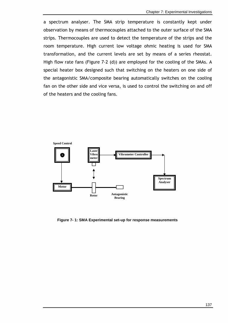
Chapter 7: Experimental Investigations
137
a spectrum analyser. The SMA strip temperature is constantly kept under
observation by means of thermocouples attached to the outer surface of the SMA
strips. Thermocouples are used to detect the temperature of the strips and the
room temperature. High current low voltage ohmic heating is used for SMA
transformation, and the current levels are set by means of a series rheostat.
High flow rate fans (Figure 7-2 (d)) are employed for the cooling of the SMAs. A
special heater box designed such that switching on the heaters on one side of
the antagonistic SMA/composite bearing automatically switches on the cooling
fan on the other side and vice versa, is used to control the switching on and off
of the heaters and the cooling fans.
Figure 7- 1: SMA Experimental set-up f or response measurements
Motor
Laser Vibrometer
Vibrometer Controller
Spectrum Analyser
Rotor
Speed Control
Antagonistic Bearing
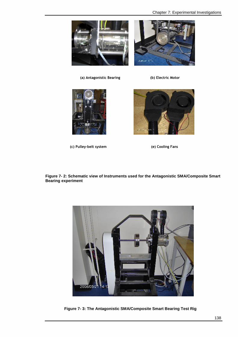
Chapter 7: Experimental Investigations
138
(a) Antagonistic Bearing (b) Electric Motor
(c) Pulley-belt system (e) Cooling Fans
Figure 7- 2: Schematic view of Instruments used for the Antagonistic SMA/Composite Smart Bearing experiment
Figure 7- 3: The Antagonistic SMA/ Composite Smart Bearing Test Rig
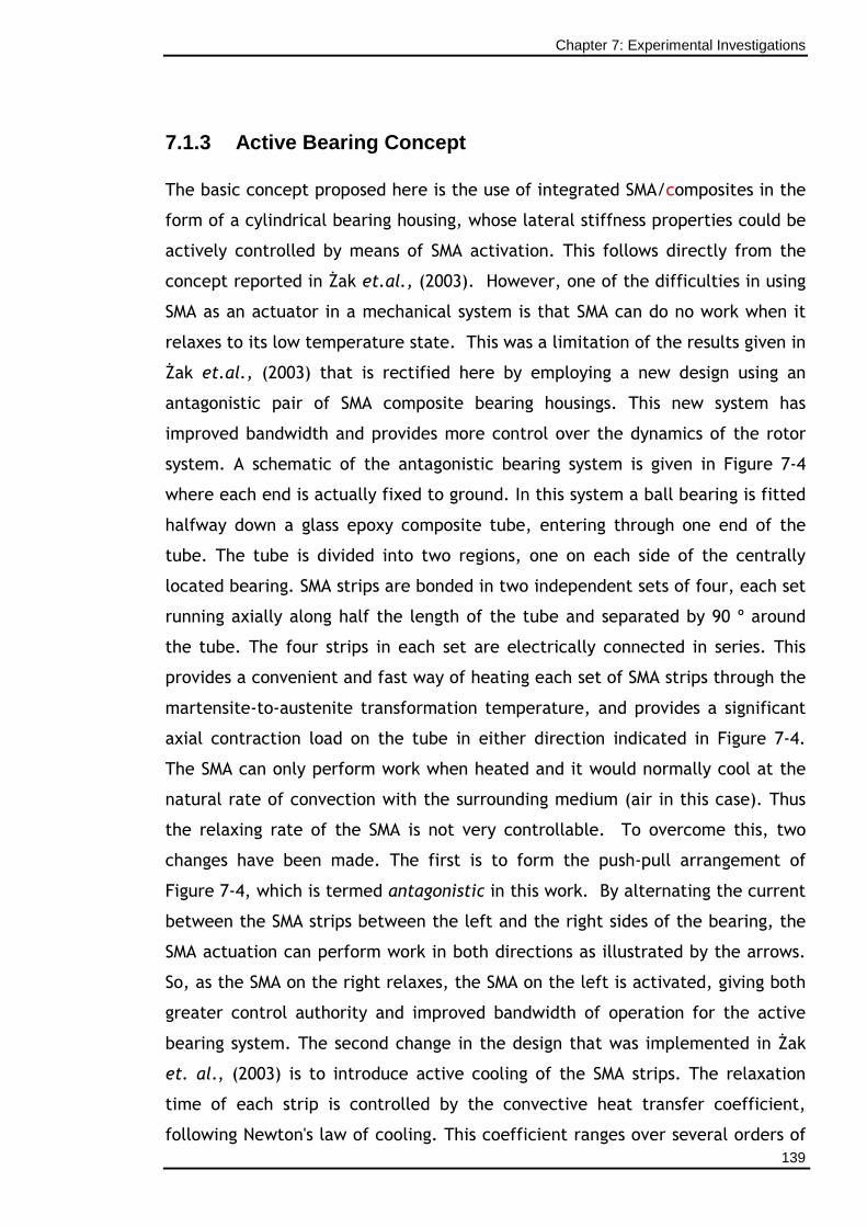
Chapter 7: Experimental Investigations
139
7.1.3 Active Bearing Concept
The basic concept proposed here is the use of integrated SMA/composites in the
form of a cylindrical bearing housing, whose lateral stiffness properties could be
actively controlled by means of SMA activation. This follows directly from the
concept reported in śak et.al., (2003). However, one of the difficulties in using
SMA as an actuator in a mechanical system is that SMA can do no work when it
relaxes to its low temperature state. This was a limitation of the results given in
śak et.al., (2003) that is rectified here by employing a new design using an
antagonistic pair of SMA composite bearing housings. This new system has
improved bandwidth and provides more control over the dynamics of the rotor
system. A schematic of the antagonistic bearing system is given in Figure 7-4
where each end is actually fixed to ground. In this system a ball bearing is fitted
halfway down a glass epoxy composite tube, entering through one end of the
tube. The tube is divided into two regions, one on each side of the centrally
located bearing. SMA strips are bonded in two independent sets of four, each set
running axially along half the length of the tube and separated by 90 º around
the tube. The four strips in each set are electrically connected in series. This
provides a convenient and fast way of heating each set of SMA strips through the
martensite-to-austenite transformation temperature, and provides a significant
axial contraction load on the tube in either direction indicated in Figure 7-4.
The SMA can only perform work when heated and it would normally cool at the
natural rate of convection with the surrounding medium (air in this case). Thus
the relaxing rate of the SMA is not very controllable. To overcome this, two
changes have been made. The first is to form the push-pull arrangement of
Figure 7-4, which is termed antagonistic in this work. By alternating the current
between the SMA strips between the left and the right sides of the bearing, the
SMA actuation can perform work in both directions as illustrated by the arrows.
So, as the SMA on the right relaxes, the SMA on the left is activated, giving both
greater control authority and improved bandwidth of operation for the active
bearing system. The second change in the design that was implemented in śak
et. al., (2003) is to introduce active cooling of the SMA strips. The relaxation
time of each strip is controlled by the convective heat transfer coefficient,
following Newton's law of cooling. This coefficient ranges over several orders of
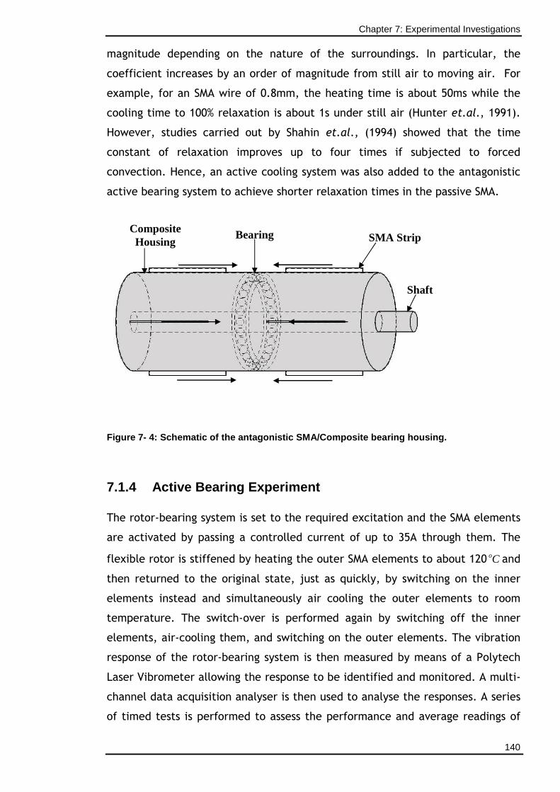
Chapter 7: Experimental Investigations
140
magnitude depending on the nature of the surroundings. In particular, the
coefficient increases by an order of magnitude from still air to moving air. For
example, for an SMA wire of 0.8mm, the heating time is about 50ms while the
cooling time to 100% relaxation is about 1s under still air (Hunter et.al., 1991).
However, studies carried out by Shahin et.al., (1994) showed that the time
constant of relaxation improves up to four times if subjected to forced
convection. Hence, an active cooling system was also added to the antagonistic
active bearing system to achieve shorter relaxation times in the passive SMA.
Figure 7- 4: Schematic of the antagonistic SMA/Comp osite bearing housing.
7.1.4 Active Bearing Experiment
The rotor-bearing system is set to the required excitation and the SMA elements
are activated by passing a controlled current of up to 35A through them. The
flexible rotor is stiffened by heating the outer SMA elements to about 120 oC and
then returned to the original state, just as quickly, by switching on the inner
elements instead and simultaneously air cooling the outer elements to room
temperature. The switch-over is performed again by switching off the inner
elements, air-cooling them, and switching on the outer elements. The vibration
response of the rotor-bearing system is then measured by means of a Polytech
Laser Vibrometer allowing the response to be identified and monitored. A multi-
channel data acquisition analyser is then used to analyse the responses. A series
of timed tests is performed to assess the performance and average readings of
Composite Housing
Shaft
Bearing SMA Strip
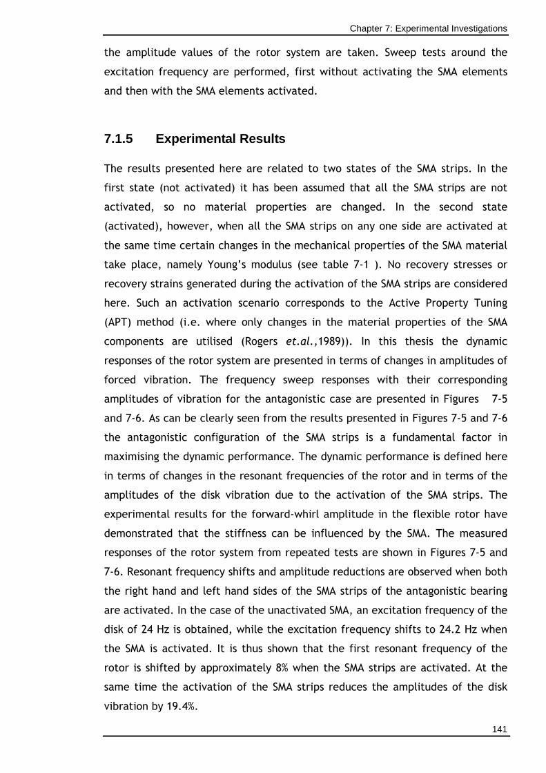
Chapter 7: Experimental Investigations
141
the amplitude values of the rotor system are taken. Sweep tests around the
excitation frequency are performed, first without activating the SMA elements
and then with the SMA elements activated.
7.1.5 Experimental Results
The results presented here are related to two states of the SMA strips. In the
first state (not activated) it has been assumed that all the SMA strips are not
activated, so no material properties are changed. In the second state
(activated), however, when all the SMA strips on any one side are activated at
the same time certain changes in the mechanical properties of the SMA material
take place, namely Young’s modulus (see table 7-1 ). No recovery stresses or
recovery strains generated during the activation of the SMA strips are considered
here. Such an activation scenario corresponds to the Active Property Tuning
(APT) method (i.e. where only changes in the material properties of the SMA
components are utilised (Rogers et.al.,1989)). In this thesis the dynamic
responses of the rotor system are presented in terms of changes in amplitudes of
forced vibration. The frequency sweep responses with their corresponding
amplitudes of vibration for the antagonistic case are presented in Figures 7-5
and 7-6. As can be clearly seen from the results presented in Figures 7-5 and 7-6
the antagonistic configuration of the SMA strips is a fundamental factor in
maximising the dynamic performance. The dynamic performance is defined here
in terms of changes in the resonant frequencies of the rotor and in terms of the
amplitudes of the disk vibration due to the activation of the SMA strips. The
experimental results for the forward-whirl amplitude in the flexible rotor have
demonstrated that the stiffness can be influenced by the SMA. The measured
responses of the rotor system from repeated tests are shown in Figures 7-5 and
7-6. Resonant frequency shifts and amplitude reductions are observed when both
the right hand and left hand sides of the SMA strips of the antagonistic bearing
are activated. In the case of the unactivated SMA, an excitation frequency of the
disk of 24 Hz is obtained, while the excitation frequency shifts to 24.2 Hz when
the SMA is activated. It is thus shown that the first resonant frequency of the
rotor is shifted by approximately 8% when the SMA strips are activated. At the
same time the activation of the SMA strips reduces the amplitudes of the disk
vibration by 19.4%.
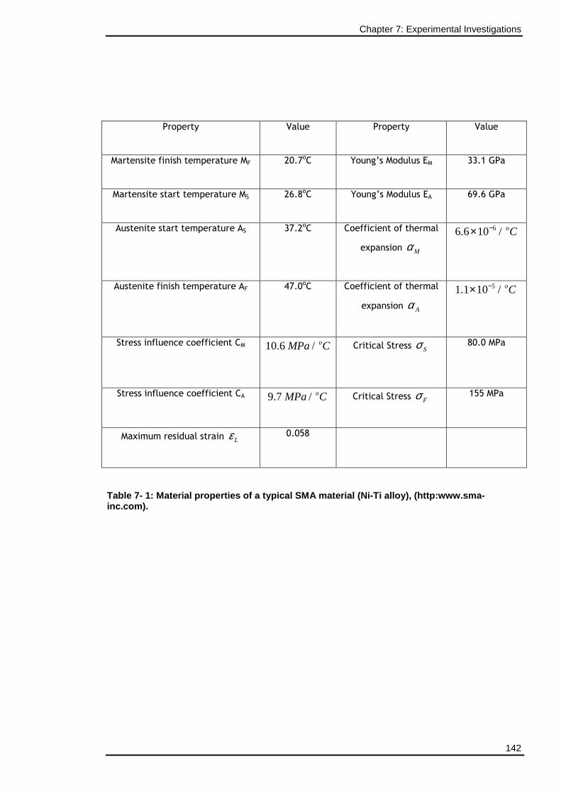
Chapter 7: Experimental Investigations
142
Property Value Property Value
Martensite finish temperature MF 20.7oC Young’s Modulus EM 33.1 GPa
Martensite start temperature MS 26.8oC Young’s Modulus EA 69.6 GPa
Austenite start temperature AS 37.2oC Coefficient of thermal
expansion Mα
66.6 10 / oC−×
Austenite finish temperature AF 47.0oC Coefficient of thermal
expansion Aα
51.1 10 / oC−×
Stress influence coefficient CM 10.6 / oMPa C
Critical Stress Sσ 80.0 MPa
Stress influence coefficient CA 9.7 / oMPa C Critical Stress Fσ 155 MPa
Maximum residual strain Lε 0.058
Table 7- 1: Material properties of a typical SMA ma terial (Ni-Ti alloy), (http:www.sma-inc.com).
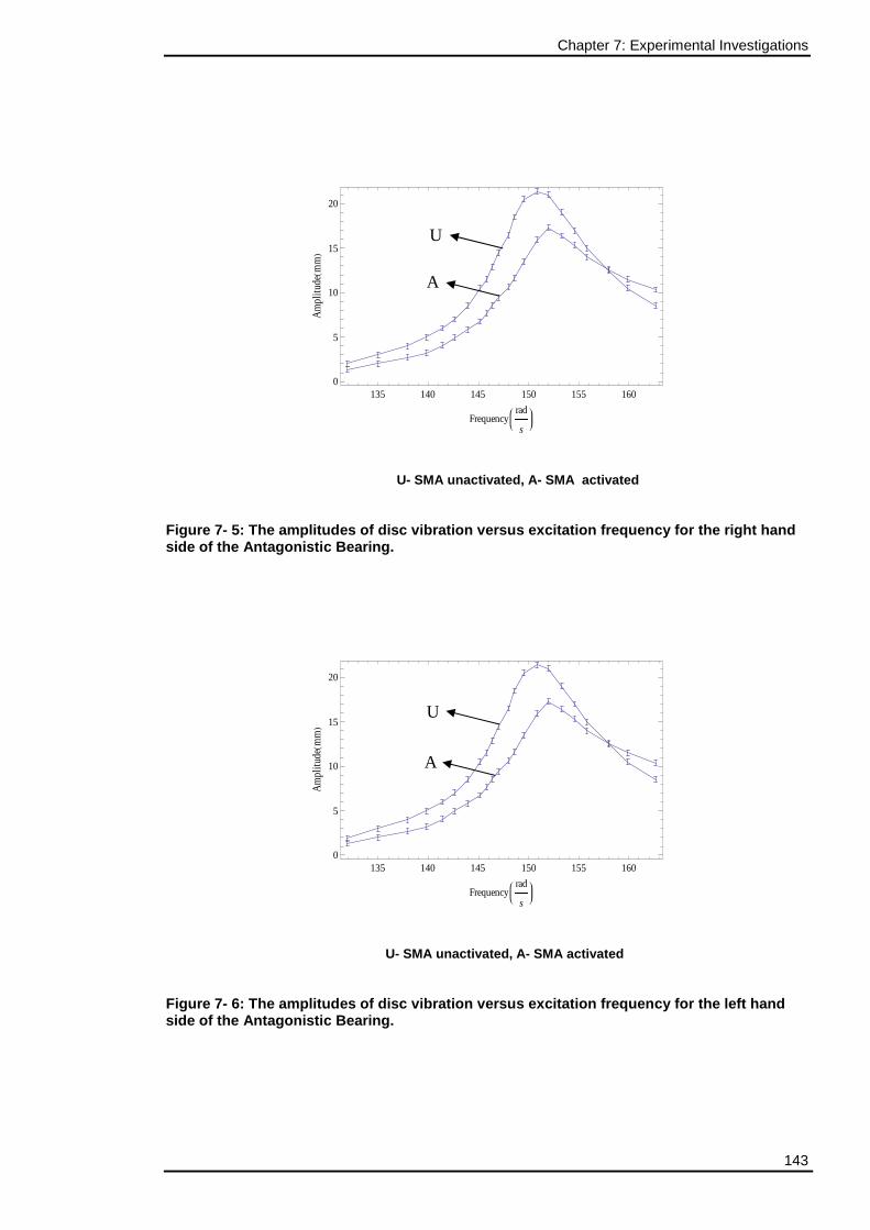
Chapter 7: Experimental Investigations
143
135 140 145 150 155 1600
5
10
15
20
Frequencyrad
s
Ampl
itudeHm
mL
U- SMA unactivated, A- SMA activated
Figure 7- 5: The amplitudes of disc vibration versu s excitation frequency for the right hand side of the Antagonistic Bearing.
135 140 145 150 155 1600
5
10
15
20
Frequencyrad
s
Ampl
itudeHm
mL
U- SMA unactivated, A- SMA activated
Figure 7- 6: The amplitudes of disc vibration versu s excitation frequency for the left hand side of the Antagonistic Bearing.
A
U
U
A
Chapter 7: Experimental Investigations
144
7.2 Controlling Flexible Rotor Vibration by means of a
Piezoelectric Stack Exciter.
7.2.1 Introduction
Unbalance forces are the main source of vibration in rotating machines, but
perfect balance is almost impossible to achieve. Moreover the distribution of
unbalance can change in time because of wear or depositions all machines are
subjected to. Reduction of rotor vibration is very important for safe and
efficient functioning of all rotating machines. This section proposes an active
vibration control scheme for controlling transverse vibration of a rotor shaft due
to mass unbalance and presents an experimental study. The use of piezoelectric
actuators in active vibration control has been considered in the past by
Palazzolo et.al., (1993) and Barret et.al., (1993). Yabuno et.al.,(2001) used a
piezoelectric actuator to stabilize the parametric resonance induced in a
cantilever beam and to control bifurcation resulting in the shift of the
bifurcation set and the expansion of the stable region. Carmignani et.al.,(2001)
developed an adaptive hydrodynamic bearing made up of a mobile housing
mounted on piezoelectric actuators. In their work they showed that imposing a
harmonic displacement on the mobile bearing, in two orthogonal directions, a
rotating force, and a correcting moment can be produced on the shaft of a rotor
system to reduce the bending caused by the unbalance. Das et.al.,(2007)
proposed an active vibration control scheme for controlling transverse vibration
of a rotor shaft due to unbalance. These authors worked on the vibration control
of rotors due to unbalance by placing electromagnetic exciters, at convenient
locations on the span of the rotor away from the bearings. They showed that,
locations distant from discs are in general convenient for exciters as they do not
interfering in any way with the rotor operation. The technique looks good
economically, as no change in the choice or design of the existing bearing or
support system of the shaft is needed. Similar electromagnetic exciters were
conceptualised by Janik et.al., (1998) and were used to excite a rotor-shaft
system for extracting the modal information by Janik et.al., (2000) and Irretier
et.al., (2002).
There are many natural phenomena in which excited parametric and self-excited
vibrations interact with one another. Examples are flow-induced vibrations and
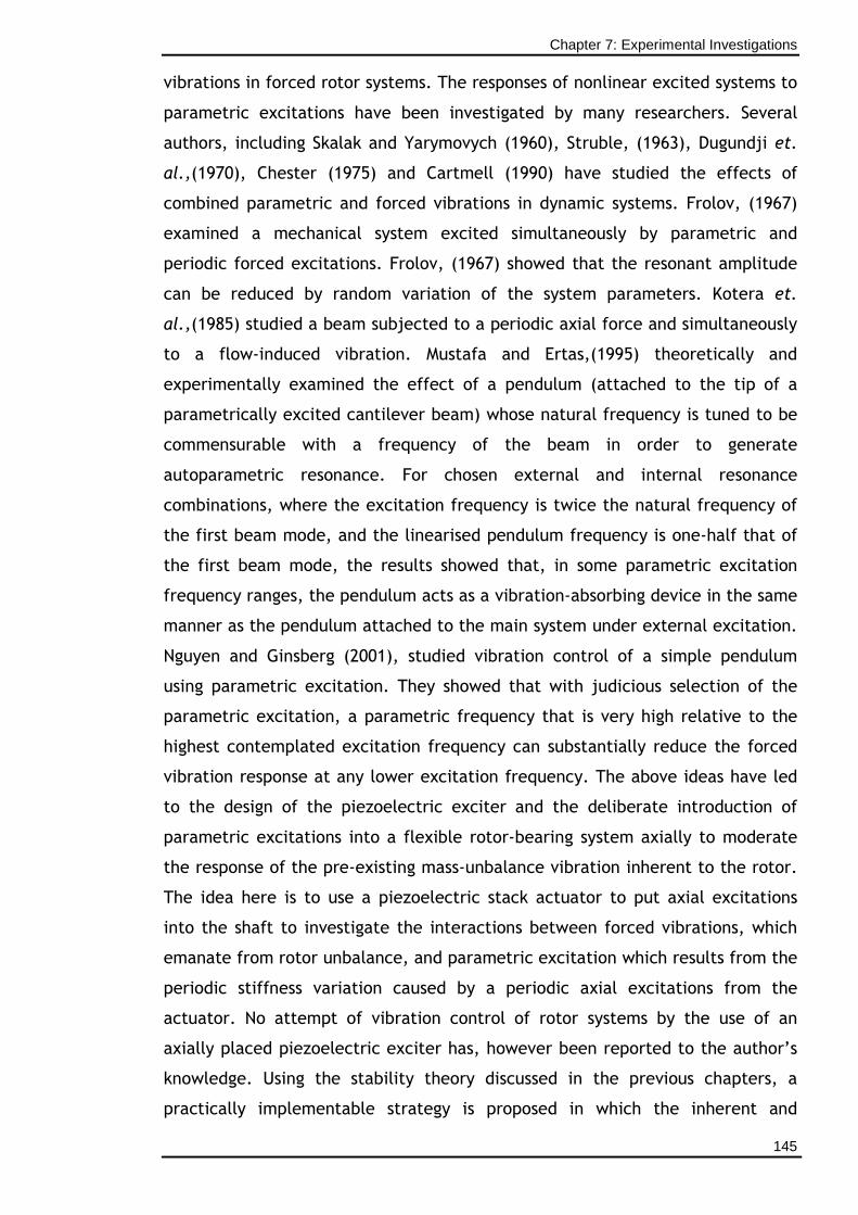
Chapter 7: Experimental Investigations
145
vibrations in forced rotor systems. The responses of nonlinear excited systems to
parametric excitations have been investigated by many researchers. Several
authors, including Skalak and Yarymovych (1960), Struble, (1963), Dugundji et.
al.,(1970), Chester (1975) and Cartmell (1990) have studied the effects of
combined parametric and forced vibrations in dynamic systems. Frolov, (1967)
examined a mechanical system excited simultaneously by parametric and
periodic forced excitations. Frolov, (1967) showed that the resonant amplitude
can be reduced by random variation of the system parameters. Kotera et.
al.,(1985) studied a beam subjected to a periodic axial force and simultaneously
to a flow-induced vibration. Mustafa and Ertas,(1995) theoretically and
experimentally examined the effect of a pendulum (attached to the tip of a
parametrically excited cantilever beam) whose natural frequency is tuned to be
commensurable with a frequency of the beam in order to generate
autoparametric resonance. For chosen external and internal resonance
combinations, where the excitation frequency is twice the natural frequency of
the first beam mode, and the linearised pendulum frequency is one-half that of
the first beam mode, the results showed that, in some parametric excitation
frequency ranges, the pendulum acts as a vibration-absorbing device in the same
manner as the pendulum attached to the main system under external excitation.
Nguyen and Ginsberg (2001), studied vibration control of a simple pendulum
using parametric excitation. They showed that with judicious selection of the
parametric excitation, a parametric frequency that is very high relative to the
highest contemplated excitation frequency can substantially reduce the forced
vibration response at any lower excitation frequency. The above ideas have led
to the design of the piezoelectric exciter and the deliberate introduction of
parametric excitations into a flexible rotor-bearing system axially to moderate
the response of the pre-existing mass-unbalance vibration inherent to the rotor.
The idea here is to use a piezoelectric stack actuator to put axial excitations
into the shaft to investigate the interactions between forced vibrations, which
emanate from rotor unbalance, and parametric excitation which results from the
periodic stiffness variation caused by a periodic axial excitations from the
actuator. No attempt of vibration control of rotor systems by the use of an
axially placed piezoelectric exciter has, however been reported to the author’s
knowledge. Using the stability theory discussed in the previous chapters, a
practically implementable strategy is proposed in which the inherent and
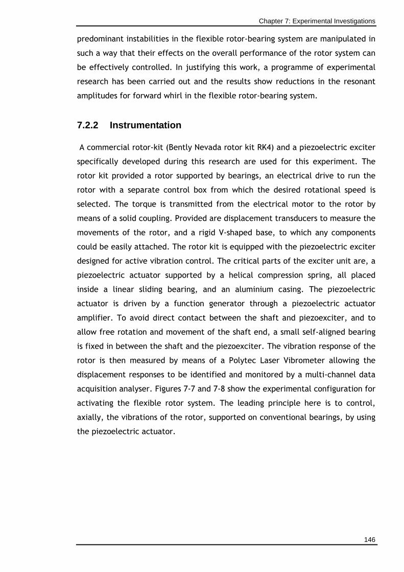
Chapter 7: Experimental Investigations
146
predominant instabilities in the flexible rotor-bearing system are manipulated in
such a way that their effects on the overall performance of the rotor system can
be effectively controlled. In justifying this work, a programme of experimental
research has been carried out and the results show reductions in the resonant
amplitudes for forward whirl in the flexible rotor-bearing system.
7.2.2 Instrumentation
A commercial rotor-kit (Bently Nevada rotor kit RK4) and a piezoelectric exciter
specifically developed during this research are used for this experiment. The
rotor kit provided a rotor supported by bearings, an electrical drive to run the
rotor with a separate control box from which the desired rotational speed is
selected. The torque is transmitted from the electrical motor to the rotor by
means of a solid coupling. Provided are displacement transducers to measure the
movements of the rotor, and a rigid V-shaped base, to which any components
could be easily attached. The rotor kit is equipped with the piezoelectric exciter
designed for active vibration control. The critical parts of the exciter unit are, a
piezoelectric actuator supported by a helical compression spring, all placed
inside a linear sliding bearing, and an aluminium casing. The piezoelectric
actuator is driven by a function generator through a piezoelectric actuator
amplifier. To avoid direct contact between the shaft and piezoexciter, and to
allow free rotation and movement of the shaft end, a small self-aligned bearing
is fixed in between the shaft and the piezoexciter. The vibration response of the
rotor is then measured by means of a Polytec Laser Vibrometer allowing the
displacement responses to be identified and monitored by a multi-channel data
acquisition analyser. Figures 7-7 and 7-8 show the experimental configuration for
activating the flexible rotor system. The leading principle here is to control,
axially, the vibrations of the rotor, supported on conventional bearings, by using
the piezoelectric actuator.
Chapter 7: Experimental Investigations
147
Figure 7- 7 : Close -up of the Piezoelectric Exciter
Figure 7- 8: Asse mbly of the Piezoexciter Test Rig
7.2.3 Design and Selection of Piezoexciter Componen t
To select a suitable piezoelectric actuator there is the need to determine the
likely force levels needed to excite the rotor parametrically, and suitable
exciters which can provide this, at appropriate levels of displacement. As the
rotor whirls there will be millimetre level axial contraction of the shaft leaving a
gap which will have to be taken up in one way or another. Use was made of the
mathematical model including the axial excitation force term developed in
Chapter 3 to find the parametric excitation force that is actually needed for the
Chapter 7: Experimental Investigations
148
rig, in order to get parametric resonances and the displacement due to the axial
contraction of the shaft. The NDSolve integrator within MathematicaTM code was
employed to solve the set of differential equations. All other parameters were
completely fixed and the parametric excitation force value was varied until a
parametric plot was obtained and the value at which the response is predicted
was taken as a threshold value for the parametric excitation force. The reader is
referred to Appendix D.1 for the obtained parametric plot. The actuator only
displaces by micrometres so there will be a potential gap between the actuator
and the shaft-end when the rotor is whirling. The actuator will therefore have to
follow the end of the shaft as it contracts, but because the other end of the
actuator has to react against something, a spring is needed to provide sufficient
reaction, and to take up the space left as the shaft contracts. Figure 7-9(a)
shows the system when the rotor is either stationary or spinning without whirl.
The design work shown in Figure 7-9 was initiated by the supervisor of this
research, with the candidate completing it and then doing the numerical
calculations. The shaft-end is fully to the right because the shaft has not
contracted due to whirl. Therefore the spring is fully compressed and exerting
its maximum force onto the shaft-end (through the actuator which is merely a
solid object transmitting that force from one side to the other (right to left)).
The maximum force available is given in equation (7.2-1),
max 2S SF k δ= (7.2- 1)
where maxSF is the maximum spring force, Sk is the spring constant, and 2δ is the
maximum spring compression.
Figure 7-9(b) shows the shaft-end having displaced to the left as a consequence
of whirl. The spring has extended to fill the gap, ∆ , and the remaining spring
compression is 1δ . This is a pre-compression and is set up via equation (7.2-2)
such that it satisfies the need for the minimum spring force ( minSF ) offered by
the spring to equal at least the maximum force which the actuator is capable of
( (max)actF ), meaning
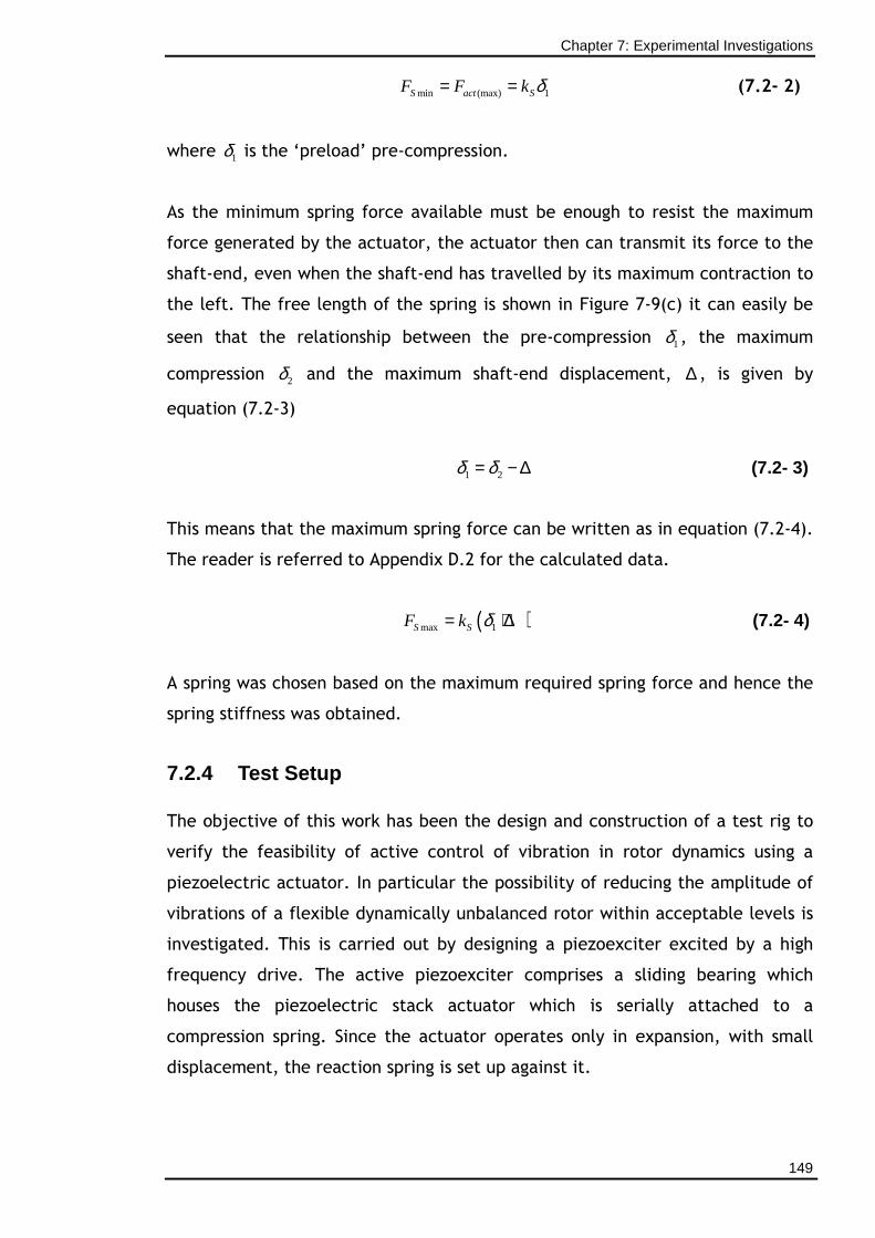
Chapter 7: Experimental Investigations
149
min (max) 1δ= =S act SF F k (7.2- 2)
where 1δ is the ‘preload’ pre-compression.
As the minimum spring force available must be enough to resist the maximum
force generated by the actuator, the actuator then can transmit its force to the
shaft-end, even when the shaft-end has travelled by its maximum contraction to
the left. The free length of the spring is shown in Figure 7-9(c) it can easily be
seen that the relationship between the pre-compression 1δ , the maximum
compression 2δ and the maximum shaft-end displacement, ∆ , is given by
equation (7.2-3)
1 2δ δ= − ∆ (7.2- 3)
This means that the maximum spring force can be written as in equation (7.2-4).
The reader is referred to Appendix D.2 for the calculated data.
( )max 1S SF k δ= + ∆ (7.2- 4)
A spring was chosen based on the maximum required spring force and hence the
spring stiffness was obtained.
7.2.4 Test Setup
The objective of this work has been the design and construction of a test rig to
verify the feasibility of active control of vibration in rotor dynamics using a
piezoelectric actuator. In particular the possibility of reducing the amplitude of
vibrations of a flexible dynamically unbalanced rotor within acceptable levels is
investigated. This is carried out by designing a piezoexciter excited by a high
frequency drive. The active piezoexciter comprises a sliding bearing which
houses the piezoelectric stack actuator which is serially attached to a
compression spring. Since the actuator operates only in expansion, with small
displacement, the reaction spring is set up against it.
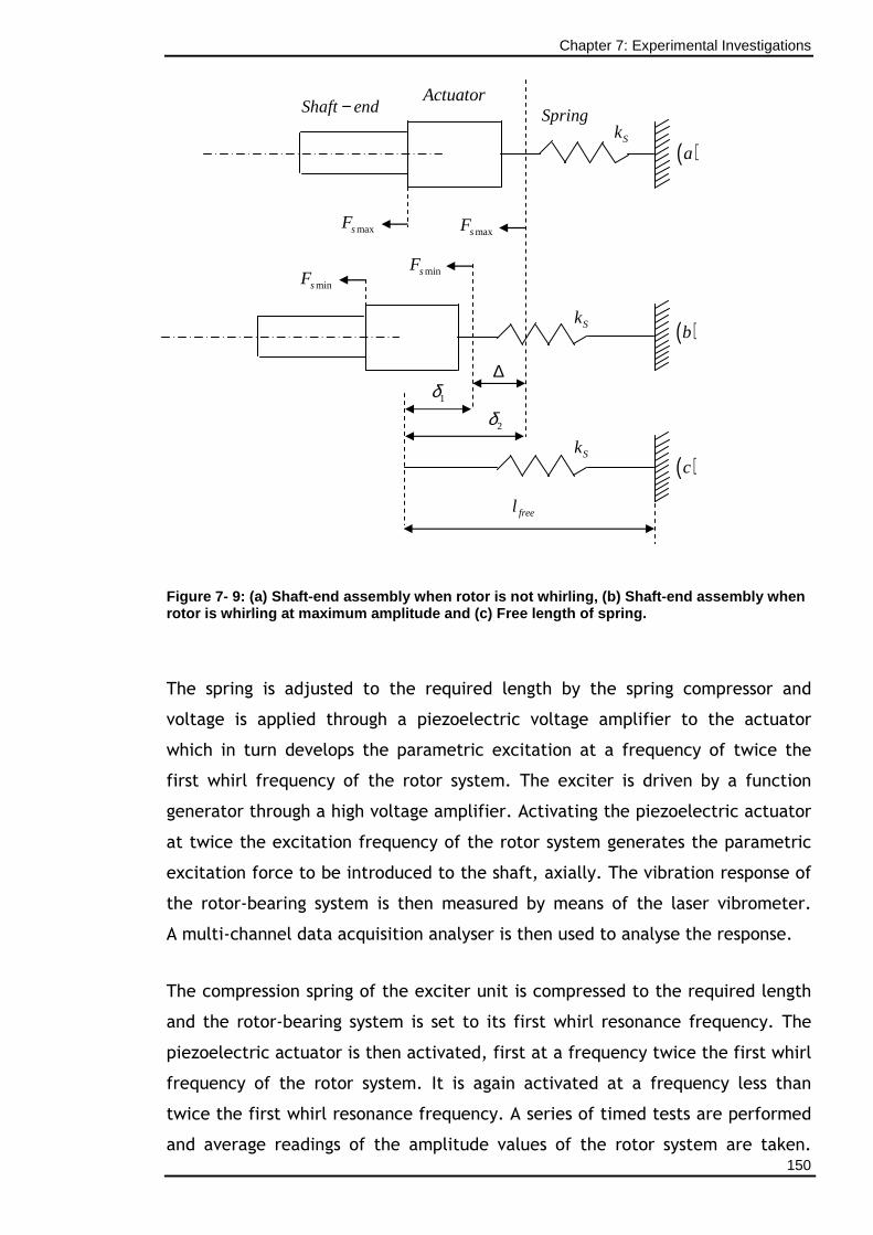
Chapter 7: Experimental Investigations
150
Figure 7- 9: (a) Shaft-end assembly when rotor is n ot whirling, (b) Shaft-end assembly when rotor is whirling at maximum amplitude and (c) Free length of spring.
The spring is adjusted to the required length by the spring compressor and
voltage is applied through a piezoelectric voltage amplifier to the actuator
which in turn develops the parametric excitation at a frequency of twice the
first whirl frequency of the rotor system. The exciter is driven by a function
generator through a high voltage amplifier. Activating the piezoelectric actuator
at twice the excitation frequency of the rotor system generates the parametric
excitation force to be introduced to the shaft, axially. The vibration response of
the rotor-bearing system is then measured by means of the laser vibrometer.
A multi-channel data acquisition analyser is then used to analyse the response.
The compression spring of the exciter unit is compressed to the required length
and the rotor-bearing system is set to its first whirl resonance frequency. The
piezoelectric actuator is then activated, first at a frequency twice the first whirl
frequency of the rotor system. It is again activated at a frequency less than
twice the first whirl resonance frequency. A series of timed tests are performed
and average readings of the amplitude values of the rotor system are taken.
Sk
minsF
maxsF maxsF
minsF
Sk
Sk
∆ 1δ
2δ
freel
Shaft end− Actuator
Spring
( )a
( )b
( )c
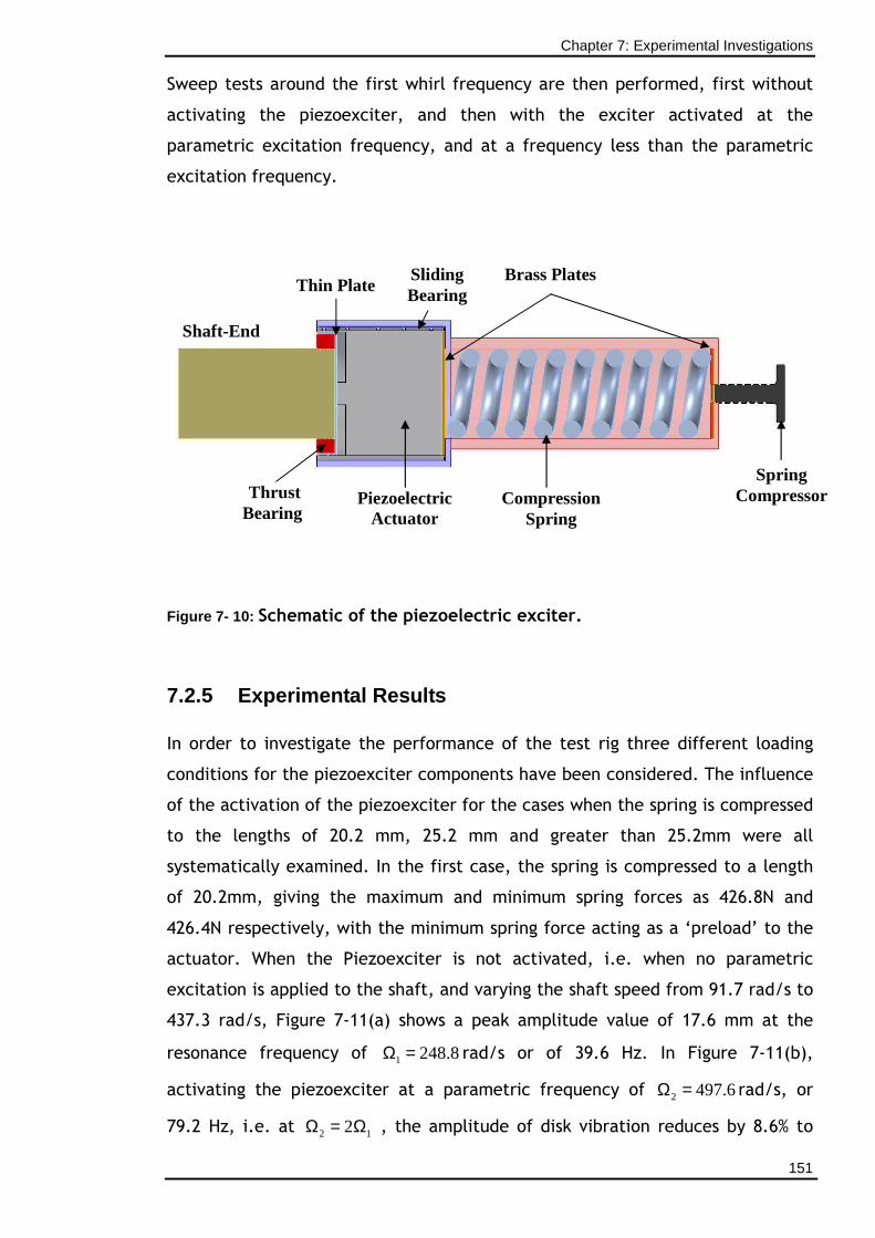
Chapter 7: Experimental Investigations
151
Sweep tests around the first whirl frequency are then performed, first without
activating the piezoexciter, and then with the exciter activated at the
parametric excitation frequency, and at a frequency less than the parametric
excitation frequency.
Figure 7- 10: Schematic of the piezoelectric exciter.
7.2.5 Experimental Results
In order to investigate the performance of the test rig three different loading
conditions for the piezoexciter components have been considered. The influence
of the activation of the piezoexciter for the cases when the spring is compressed
to the lengths of 20.2 mm, 25.2 mm and greater than 25.2mm were all
systematically examined. In the first case, the spring is compressed to a length
of 20.2mm, giving the maximum and minimum spring forces as 426.8N and
426.4N respectively, with the minimum spring force acting as a ‘preload’ to the
actuator. When the Piezoexciter is not activated, i.e. when no parametric
excitation is applied to the shaft, and varying the shaft speed from 91.7 rad/s to
437.3 rad/s, Figure 7-11(a) shows a peak amplitude value of 17.6 mm at the
resonance frequency of 1 248.8Ω = rad/s or of 39.6 Hz. In Figure 7-11(b),
activating the piezoexciter at a parametric frequency of 2 497.6Ω = rad/s, or
79.2 Hz, i.e. at 2 12Ω = Ω , the amplitude of disk vibration reduces by 8.6% to
Shaft-End
Thrust Bearing
Thin Plate Sliding Bearing
Brass Plates
Piezoelectric Actuator
Compression Spring
Spring Compressor
Chapter 7: Experimental Investigations
152
16mm. However, in Figure 7-11(c) activating the piezoexciter at an arbitrarily
chosen parametric frequency of 450 rad/s i.e. at 2 12Ω < Ω increases the
amplitude of the disk vibration by 10.4% to 19.3mm.
In the second case, the spring is compressed to a length of 25.2mm, giving the
maximum and minimum spring forces as 532.5N and 532N respectively,
Figure 7-12(a) shows the peak amplitude of the disk vibration to be 15mm at the
resonance frequency of 1 248.8Ω = rad/s, or 39.6 Hz. Activating the piezoexciter
at the parametric frequency of 2 497.6Ω = rad/s, or 79.2 Hz, i.e. at 2 12Ω = Ω ,
Figure 7-12(b) shows that the amplitude of disk vibration reduces by 13% to
13mm, which is a 4.4% increase in comparison with the previous case. Also
activating the piezoexciter at an arbitrarily chosen parametric frequency of 450
rad/s, i.e. at 2 12Ω < Ω , Figure 7-12(c) shows an increase in the amplitude of the
disk by 10% to 16.5mm.
In the third case when spring is compressed at lengths greater than 25.2 mm,
activating the piezoexciter showed no visible changes in the amplitudes of
vibrations.
The experimental investigations show the same trend as explained in earlier
chapters that the introduction of axial parametric excitation to a flexible rotor,
which is also susceptible to mass unbalance, influences the amplitude of
vibration of the disk. The greatest dynamic performance is obtained for the case
when the spring is compressed to a length of 25.2mm, and on activating the
piezoexciter, there was seen to be a reduction of 13% in the amplitude value at
principal parametric resonance. On the other hand, an increase in amplitude
value was observed when the exciter was activated at a parametric excitation
frequency of less than twice the first whirl resonance frequency of the shaft.
However, at a spring compression of 20.2mm, on activating the exciter, there
was a reduction of 8.6% in amplitude at a parametric resonance of twice the
resonance frequency of the shaft. Also, a higher increase in amplitude was
observed when the exciter was activated at a parametric frequency less than
twice the first whirl resonance frequency of the shaft at the spring length of
20.2mm. Making the compression length more than 25.2mm had no visible effect
on the amplitude of vibration.
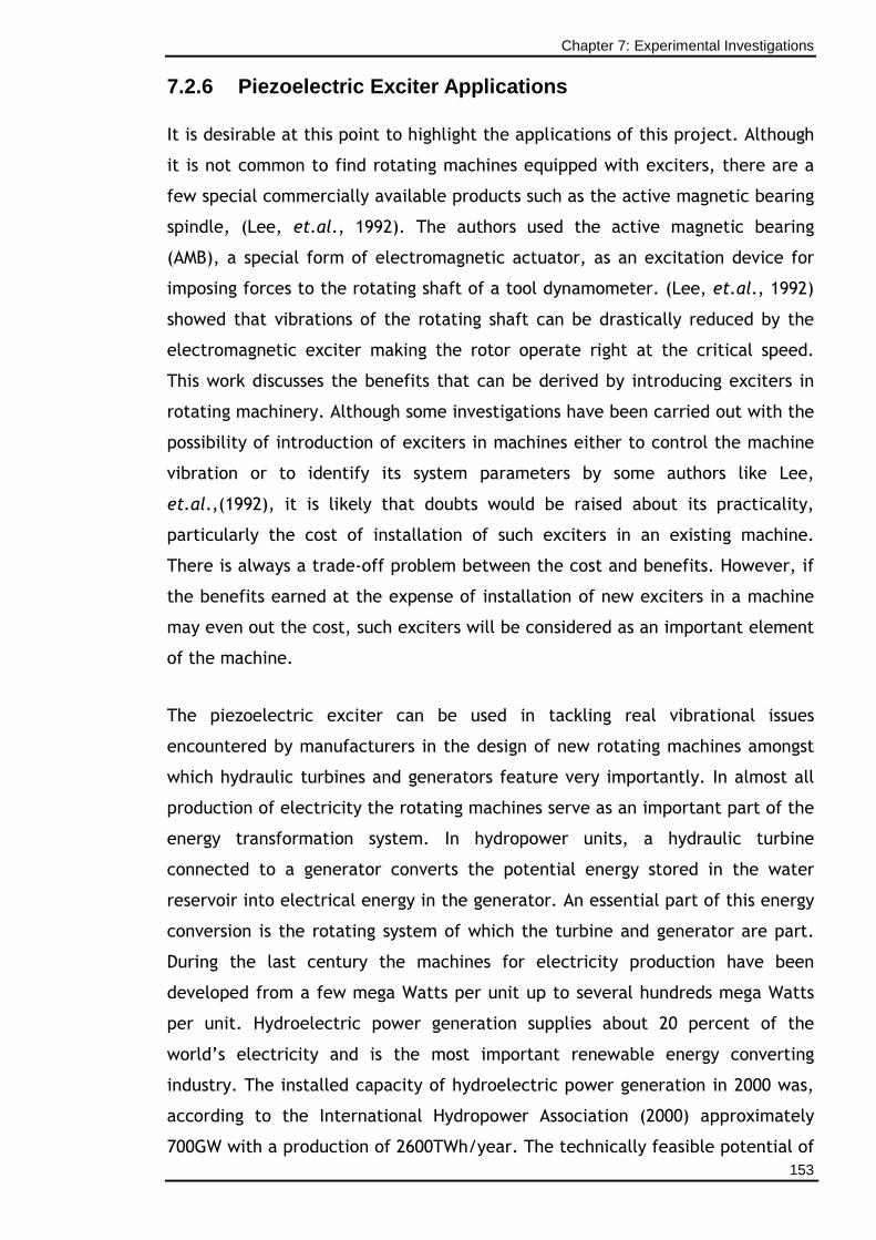
Chapter 7: Experimental Investigations
153
7.2.6 Piezoelectric Exciter Applications
It is desirable at this point to highlight the applications of this project. Although
it is not common to find rotating machines equipped with exciters, there are a
few special commercially available products such as the active magnetic bearing
spindle, (Lee, et.al., 1992). The authors used the active magnetic bearing
(AMB), a special form of electromagnetic actuator, as an excitation device for
imposing forces to the rotating shaft of a tool dynamometer. (Lee, et.al., 1992)
showed that vibrations of the rotating shaft can be drastically reduced by the
electromagnetic exciter making the rotor operate right at the critical speed.
This work discusses the benefits that can be derived by introducing exciters in
rotating machinery. Although some investigations have been carried out with the
possibility of introduction of exciters in machines either to control the machine
vibration or to identify its system parameters by some authors like Lee,
et.al.,(1992), it is likely that doubts would be raised about its practicality,
particularly the cost of installation of such exciters in an existing machine.
There is always a trade-off problem between the cost and benefits. However, if
the benefits earned at the expense of installation of new exciters in a machine
may even out the cost, such exciters will be considered as an important element
of the machine.
The piezoelectric exciter can be used in tackling real vibrational issues
encountered by manufacturers in the design of new rotating machines amongst
which hydraulic turbines and generators feature very importantly. In almost all
production of electricity the rotating machines serve as an important part of the
energy transformation system. In hydropower units, a hydraulic turbine
connected to a generator converts the potential energy stored in the water
reservoir into electrical energy in the generator. An essential part of this energy
conversion is the rotating system of which the turbine and generator are part.
During the last century the machines for electricity production have been
developed from a few mega Watts per unit up to several hundreds mega Watts
per unit. Hydroelectric power generation supplies about 20 percent of the
world’s electricity and is the most important renewable energy converting
industry. The installed capacity of hydroelectric power generation in 2000 was,
according to the International Hydropower Association (2000) approximately
700GW with a production of 2600TWh/year. The technically feasible potential of
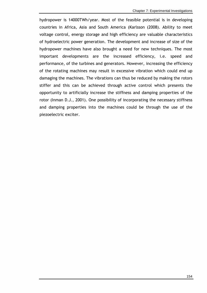
Chapter 7: Experimental Investigations
154
hydropower is 14000TWh/year. Most of the feasible potential is in developing
countries in Africa, Asia and South America (Karlsson (2008). Ability to meet
voltage control, energy storage and high efficiency are valuable characteristics
of hydroelectric power generation. The development and increase of size of the
hydropower machines have also brought a need for new techniques. The most
important developments are the increased efficiency, i.e. speed and
performance, of the turbines and generators. However, increasing the efficiency
of the rotating machines may result in excessive vibration which could end up
damaging the machines. The vibrations can thus be reduced by making the rotors
stiffer and this can be achieved through active control which presents the
opportunity to artificially increase the stiffness and damping properties of the
rotor (Inman D.J., 2001). One possibility of incorporating the necessary stiffness
and damping properties into the machines could be through the use of the
piezoelectric exciter.
Chapter 7: Experimental Investigations
155
100 150 200 250 300 350 40013
14
15
16
17
Frequencyrad
sAm
plitu
deHm
mL
(a) Piezoexciter Unactivated
100 150 200 250 300 350 40012
13
14
15
16
Frequencyrad
s
Ampl
itudeHm
mL
(b) Piezoexciter activated at 2 12Ω = Ω
100 150 200 250 300 350 40015
16
17
18
19
Frequencyrad
s
Ampl
itudeHm
mL
(c) Piezoexciter activated at 2 12Ω < Ω
Figure 7- 11: The amplitudes of disc vibration vers us frequency with a spring compression length of 20.2mm.
Chapter 7: Experimental Investigations
156
100 150 200 250 300 350 40011.5
12.0
12.5
13.0
13.5
14.0
14.5
15.0
Frequencyrad
sAm
plitu
deHm
mL
(a) Piezoexciter Unactivated
100 150 200 250 300 350 40010.0
10.5
11.0
11.5
12.0
12.5
13.0
Frequencyrad
s
Ampl
itudeHm
mL
(b) Piezoexciter activated at 2 12Ω = Ω
100 150 200 250 300 350 40012
13
14
15
16
Frequencyrad
s
Ampl
itudeHm
mL
(c) Piezoexciter activated at 2 12Ω < Ω
Figure 7- 12: The amplitudes of disc vibration vers us frequency with a spring compression length of 25.2mm.
Chapter 8: Discussions of Results
157
CHAPTER 8
DISCUSSIONS OF RESULTS
_________________________________________________
8.1 Introduction
The theoretical and experimental analyses for the flexible rotor system have
been presented in Chapters 3 to 7. The derivation of the mathematical models
for the rotor system was discussed in Chapter 3. The analytical and numerical
techniques, including the method of multiple scales and direct numerical
integration by the use of MathematicaTM, for the prediction of the response of
the presented models as shown in Figures 3-1 to 3-5 were presented in Chapter
4. Chapter 5 presents a steady-state stability analysis of the rotor system via the
Routh-Hurwitz stability criterion using the nonautonomous equations obtained
from the multiple scales analysis in Chapter 4. A numerical study into the
system’s dynamics was extended in Chapter 6, where a study of the bifurcations
and stability of the solutions via phase planes, Poincaré maps, time plots,
bifurcation diagrams and the Lyapunov exponent were summarised. Chapter 7
summarised the novel methods of an antagonistic SMA/Composite bearing and a
piezoelectric exciter for the control and reduction of vibration amplitudes in the
flexible rotor system. The purpose of this chapter is to examine and extend the
discussions where appropriate, the results from Chapters 3 to 7, allowing
conclusions to be derived from the respective results.
8.2 Analytical Results
Mathematical models for the rotor system are proposed for vibration analysis
and control. In the following are summarised points from the studies:
• Initially, the particular structure under investigation was a Jeffcott like
flexible rotor system for which the systems kinematics are presented. The
system equations were derived by first constructing the kinetic and strain
energies of the rotor elements, followed by the formation of the virtual
Chapter 8: Discussions of Results
158
work of external forces, including, bearing and axial forces.
Rayleigh-Ritz method and Lagrange’s equations were then applied to the
obtained expressions resulting in coupled differential equations.
• The axial force terms included in the equations of motion provide a means
for axially directed harmonic force to be introduced into the system,
noting that this is not a follower force and that it maintains the line of
the undisturbed equilibrium axis.
The analytical developments involved using the methods of multiple scales and
direct numerical integration. In the following are summarised points which
emerge from these studies:
The results from the method of multiple scales in Figures 4-1 to 4-4 showed good
conclusive results for the cases of not including parametric force terms but
increasing the mass unbalance and the damping coefficient, and including
parametric force terms. The effect of increasing the mass unbalance of the rotor
system does indeed have a global effect on the nonlinear response of the overall
system. The response amplitudes increase as the mass unbalance increases.
Increasing the damping coefficient results in decreases in the amplitudes, but
the decreases are very small and do not cause the elimination of the jump
phenomena.
Including parametric force terms in the equations tend to reduce the peak whirl
amplitudes of the whirling motion by approximately 23% and eliminate the jump
in the rotating speed.
Numerically integrating the governing equations of motion (3.2-85) and (3.2-86)
within MathematicaTM has produced results that corroborate those of the
method of multiple scales. There is evidence of consistent phenomenon whereby
both the responses in the first mode for 1q and 2q show a characteristic
hardening effect and a jump phenomena, and reduction in the peak amplitudes
when parametric excitation terms are introduced into the system.
Chapter 8: Discussions of Results
159
The numerical integration results give the response for the first mode only
whereas the method of multiple scales generates results related to the chosen
resonance condition and around the region of perfect external tuning, by means
of the detuning parameter, εσ (equation 4.2-41).
8.3 Stability Analysis Results
In performing the stability analysis, the governing differential equations were
solved analytically using the method of multiple scales and the ensuing
nonautonomous slow-time modulation equations were used to construct a
stability matrix and the stability of the system was then analysed using the
Routh-Hurwitz stability criterion. The results show that there are values of mass
unbalance for which the system can be stable or unstable.
Figures 5-1 and 5-2 and Table 5-1 give a summary of the stability of the steady-
state solutions as the mass unbalance is varied. The results show that at mass
unbalances of 0.004=um kg the system’s motion is stable and increasing the mass
unbalances to 3 um , 4 um and 5 um the motion becomes unstable. Also, further
increase of the mass unbalance values to 6 um and 7 um makes the motion stable
again.
From Figures 5-1 and 5-2, at mass unbalance values between zero and 0.006kg,
the system shows stable motions. At mass unbalance values from 0.006 to
0.022kg, the system is unstable and at mass unbalances greater than 0.022kg the
system’s motion again becomes stable.
The above results emphasize the intuitive expectation that mass unbalance
affects the rotor system’s stability under certain conditions.
8.4 Numerical Results
The subsequent numerical analyses were undertaken by generating problem-
specific code within the public-domain software Dynamics 2.
Chapter 8: Discussions of Results
160
Figure 6-2 gives plot of nondimensionalised bifurcatory behaviour of amplitude
response as a function of the excitation frequency Ω . For the first response
mode, it can be deduced that increase in the mass unbalance causes increase in
the amplitude of vibration and shifts the amplitude peak more to the right
mirroring the effects noticeable in the results of the multiple scales.
The calculated Lyapunov exponent supports the notion that nonlinearities can
generate undesirable responses like chaos, but only in cases of very a high
excitation level. However, no route to chaos is indicated in the plots of Figure 6-
2.
Figure 6-3 shows the bifurcatory behaviour of the amplitude response in the x-
direction as a function of nondimensionalised excitation acceleration,
accompanied by its respective Lyapunov exponent. For the linear response from
chapters 4 to 7, ( 0.004um kg= ), a periodic response for a wide range of
excitation values is achieved. As the mass unbalance is increased, evidence of
chaos surfaces.
The results in Figures 6-3(b), 6-3(c) and 6-3(d) show period doubling bifurcations
as mass unbalance increases. In addition, a jump up to the zero level in the
Lyapunov exponent plots occur, and indicates that the system has moved to
higher period multiples.
Figure 6-4 shows the bifurcatory behaviour of the amplitude response in the x-
direction as a function of normalised excitation acceleration accompanied by its
respective Lyapunov exponent for the case of the introduced parametric
excitation term. The results show stable periodic motions, indicating that all the
period doubling and unstable motions observed in Figure 6-3 have become stable
motions with the introduction of the parametric excitation term at the principal
parametric resonance.
At discrete nondimensionalised excitation acceleration points of the
bifurcations in Figures 6-3 and 6-4, phase planes, Poincaré maps and time plots
are given in Figures 6-5 to 6-11. The following are general observations of the
flexible rotor system as the mass unbalance is increased from um to 5 um :
Chapter 8: Discussions of Results
161
• The periodic orbits in the phase planes move away from each other as the
effect of the predominant systems nonlinearity is increased by
manipulation of the mass unbalance, thus by the excitation acceleration.
And therefore, the phenomena behind this behaviour, as shown on the
phase planes, could represent a bifurcation to chaos.
• Complicated phase plots are obtained for higher values of mass
unbalance, indicating likely chaotic motions as the system effectively
becomes more nonlinear.
• In Figures 6-7(d), 6-8(c) and 6-9(b) strange attractors are obtained for the
Poincaré maps for higher values of mass unbalance, again indicating likely
chaotic motions.
• With the introduction of parametric excitation terms, the phase planes,
Poincaré maps and time plots at the discrete nondimensionalised
excitation acceleration points display periodic motions indicating stability
or stable motions.
Figures 6-12 to 6-17 show the nonlinear dynamic system analyses by the use of
specialised code written in MathematicaTM as the mass unbalance increases from
um to 5 um :
• For all the discrete mass unbalance values, the motion is stable and
periodic in the flexible rotor system.
• The Poincaré map converges to darker areas towards a point indicating a
period one motion.
• Using the NDSolve integrator within MathematicaTM in analysing the
bifurcation plots in Figure 6-3 at nondimensionalised excitation
accelerations of 618, 505 and 460 for mass unbalance values of 3 um , 4 um
and 5 um respectively, (i.e. for higher values of mass unbalance)
complicated phase plots are obtained, and strange attractors are also
obtained for the Poincaré maps (Figure 6-17), all indicating likely chaotic
motions.
Chapter 8: Discussions of Results
162
8.5 Experimental Results
The following results were obtained from two experimental programmes carried
out on different flexible rotor systems. Vibrations in industrial rotating
machines, can, for certain rotational speed, be so violent that they can cause
significant damage, and the following are the resultant effects of introducing
excitations axially into the shaft of such rotating machines using two types of
smart material technologies, namely Shape Memory Alloys and Piezoactuators, in
the forms of antagonistic SMA/Composite active bearing and Piezoelectric
exciters respectively.
• The antagonistic SMA effect was successfully applied to control stiffness
of a rotor bearing housing, and to manipulate the natural frequencies of
the rotor system. The experimental results for the forward-whirl
amplitude in the rotor system have demonstrated that the stiffness can be
usefully affected by the SMA, with around a 19.4% reduction in the critical
whirl amplitude.
• The piezoelectric exciter was successfully used to introduce parametric
excitations into a second rotor system. The combined effects due to the
existing forced vibration due to mass unbalance and also an additional
parametric excitation in principal parametric resonance provided by the
piezoexciter resulted in a more linear response than that provided by the
rotor system alone. This has led to the moderation of the responses of the
pre-existing mass unbalance vibration inherent to the rotor, with an
approximately 13% reduction in the critical whirl amplitude.
8.6 Conclusions
The first three methods of investigating and identifying the response behaviour
of rotor systems have all shown similar trends with regards to the effects of
increasing the mass unbalance and introducing parametric force terms.
Numerical studies have also indicated that chaos is evident as the system
becomes more nonlinear due to the increase in mass unbalance and that with
the introduction of parametric excitation terms the system’s motion becomes
Chapter 8: Discussions of Results
163
periodic. Prototypical experimental results from tests on rotor systems conclude
that the novel antagonistic bearing and piezoelectric exciter concepts could be
successfully applied to industrial applications, particularly installations where
axial loading on the rotor shaft is also an inherent part of the control actuation.
Chapter 9: Conclusions and Recommendations for Further Work
164
CHAPTER 9
CONCLUSIONS AND RECOMMENDATIONS FOR FURTHER WORK
_________________________________________________
9.1 Summary
The research described in this thesis has been concerned with the issue of
dynamic response modifications within flexible rotor systems by the use of Smart
Materials in the form of shape memory alloys and piezoelectric actuators. The
techniques that have been developed are based on the exploitation of the
mitigating effects of a SMA/composite antagonistic bearing and piezoelectric
exciters on the over all system response. It has been shown theoretically that
certain nonlinear effects can be advantageously neutralised with the novel
methodologies of introducing axial forces parametrically and through an active
bearing component. It has been demonstrated in two different experiments,
using different flexible rotor systems that the stiffness of the shaft can be
usefully influenced by SMA and piezoelectric actuators. For a laboratory rotor
system supported on two bearings, one of which was a two sided active
component comprising a composite tube with specially configured and
integrated SMA strips termed “antagonistic” in this work, the critical speed was
usefully shifted about its normal value and the whirling amplitude reduced
drastically. The antagonistic SMA effect was successfully applied to control the
stiffness of a rotor bearing housing, and hence to manipulate the natural
frequency of the rotor system. It has also been demonstrated that fitting a
piezoexciter for axial excitation of the rotor, has greatly influenced the overall
nonlinear response of the rotor system. There are some limited references to
such systems in the literature but there have not been many reported
phenomena relating to the design and application of bespoke antagonistic
SMA/composite active bearings and axial piezoelectric exciter for the control of
vibration in flexible rotors.
Chapter 9: Conclusions and Recommendations for Further Work
165
In order to gain an understanding of the behaviour of the flexible rotor system
subjected to excitations due to rotating mass unbalance, it was decided firstly
to develop an analytical model of which axial forces could be introduced into
the system through an axial force term, and the equations were derived in the
form of the well known Duffing equation. This can be used to determine the
critical whirling amplitude in the rotor system with and without the introduction
of the axial forces. These equations were solved analytically, to second order
approximation, and the nonlinear vibration solutions were investigated when it
was subjected to transverse vibration, using the method of multiple scales, and
they were also numerically integrated by the use of NDSolve within
MathematicaTM. Interesting nonlinear and interactive behaviour was observed for
the primary resonance condition, 1 εσωΩ = + , and for the parametric resonance
condition, 2 2 εσωΩ = + when parametric excitations were deliberately
introduced into the rotor system, where, Ω is the primary resonance frequency,
2Ω is the parametric excitation frequency and εσ is the internal detuning
parameter. In this research it has been shown conclusively by using a second
order multiple scales approximation that the nonlinear characteristics of the
steady-state responses to the nonautonomous modulation equations can be
manipulated by altering the mass unbalance and also by the introduction of a
parametric force term. In particular it was shown that the effect of increasing
the mass unbalance increases the amplitude of vibration. Further more, it was
found that increasing the damping coefficient gives a very small decrease in the
whirl amplitude of vibration. In addition to this, including a parametric force
term results in the decrease in the amplitudes of vibration, effectively
linearising the sub-system response amplitudes (Figure 4-4), notwithstanding the
fact that such numerical relationships are necessarily system-data specific.
Stability of steady-state solutions analysis was performed for the rotor system.
Nonautonomous equations taken from the multiple scales analysis were used for
the analysis. Characteristics equation formed from the determinant of the
equations was analysed using Routh-Hurwitz criterion for stability analysis. From
the analysis a variety of stability information was extracted. Stability table and
plots were obtained for various mass unbalance values and it was observed that
Chapter 9: Conclusions and Recommendations for Further Work
166
for certain increased values of mass unbalance the system becomes unstable and
as it increases further the system becomes stable.
The effects were corroborated numerically and a further study of the
bifurcations and stability of the solutions via phase planes, Poincaré maps, time
plots, bifurcation diagrams and Lyapunov exponents showed that additional, and
highly complex, dynamics could be observed, particularly in more strongly
excited systems. A range of numerical results were obtained for both the second
order analytical approximation and numerical integrations for the model of a
rotor system in the physical co-ordinate space, and these underpinned the
general finding that response amplitude characteristics could be effectively
linearised and controlled for different combinations of data. This suggests that
the useful mitigating effect might also be realisable in the more complex rotor
system and so parallel programmes of experimental tests were carried out.
The response characteristics of physical industrial applications were thus
determined. A rotor system is considered a vibrating system in the classical
sense, and its excitations can be due to rotating mass unbalance. A resonance
condition exists when the frequency of excitation due to the mass unbalance
coincides with the natural frequency, which tends to increase the amplitude of
vibration of the system. To find a practical design solution to the effects of
nonlinear responses, it was first necessary to change the frequencies of the shaft
rotor system, to avoid critical speeds whilst running up and running down rotors,
and to control the vibration levels or rotor stresses in a rotating machine. The
effect of this response of building one of two bearings of the rotor system into
an active SMA/Composite antagonistic bearing and also deliberately introducing
parametric resonance axially into the shaft of a second rotor system were also
assessed. It was found that in the case of the antagonistic bearing, the fact that
the bearing was fitted within the tube, half-way along, introduced the local
dynamics of the tube into the dynamic end conditions of the rotor, and these
dynamics were controlled by means of the embedded SMA strips. The SMA effect
was thus applied to control the stiffness of the rotor bearing housing, and hence
to manipulate the natural frequencies of the rotor system, and used to reduce
the critical whirl amplitude. In the case of introducing parametric excitations
into a flexible rotor system by means of a piezoexciter, it was found that the
Chapter 9: Conclusions and Recommendations for Further Work
167
responses of the pre-existed mass unbalance vibration got moderated and
resulted in the reduction of the critical whirl amplitude when the exciter was
excited parametrically at the principal parametric resonance.
This research provides some basic theory and understanding of how nonlinear
and unstable rotor systems can be made more efficient and stable. The practical
goal had been to try to control vibration, by reducing the whirl amplitude of the
vibrating system. This was tackled by means of using (a) integrated
SMA/composites in the form of a cylindrical antagonistic bearing housing
component, who’s radial and stiffness properties could be actively controlled by
means of SMA actuation, and together with an additional axial force component
as a result of SMA action on the rotor, (b) piezoelectric exciter fitted to the
shaft of the rotor for parametric axial excitation of the rotor whose effects may
be used to moderate the responses of the pre-existing mass unbalance vibration
inherent to the rotor.
Engineers and scientists are encouraged to use these new approaches with prior
understanding of the behaviour of rotating machines under the influence of mass
unbalance. By obtaining a good basic understanding of each individual
component, an ideal and robust overall linear and stable system can ultimately
be configured and hence more reliable and efficient industrial systems can be
designed.
9.2 Recommendations for Further Work
It would be good to develop a binary control strategy for the antagonistic active
bearing and to check the performance for the flexible rotor at the first critical
and possibly higher whirl speeds.
Then to investigate how such binary control can be integrated within a model-
based controller (noting that the two-state behaviour is a fundamental feature
of SMAs) so that the versatility of control is maximised both at critical speeds
and above. This will require a minimised time constant for the antagonistic
active bearing, which will, in turn, need maximised heating and cooling rates.
This could introduce problems of thermal fatigue in the composite and
Chapter 9: Conclusions and Recommendations for Further Work
168
particularly in the epoxy adhesive used to secure the SMA strips, and these will
have to be investigated.
The experimental test rig could be modified to an overhung configuration, in
which gyroscopic forces will be highly significant, and then to see how backward
travelling whirl can be mitigated at the first, and possibly higher, critical
speeds, with attendant implications for the reduction of cyclic stress effects.
The experimental test rig for the piezoexciter case could also be modified and
parametric excitations introduced axially at both ends of the shaft into the
system to examine the combination effects on the system.
References
169
REFERENCES
_________________________________________________
Abduljabbar Z., ELMadany M.M., and AlAbdulwahab A.A.,(1996), Computers and
Structures,58(3),pp.499-511,Active Vibration Control of a Flexible Rotor.
Active Materials Laboratory, MIT, USA. http://aml.seas.ucla.edu
AdaptaMat, Finland (MSM actuators).
Adiletta G., Guido A., and Rossi R. C., (1996), Nonlinear Dynamics, 10, pp. 251-
269, Chaotic motions of a rigid rotor in short journal bearings.
Adiletta G., Guido A., and Rossi R. C., (1997a), Nonlinear Dynamics, 14, pp. 57-
87, Nonlinear dynamics of a rigid unbalanced rotor in short bearings, Part I:
Theoretical analysis.
Adiletta G., Guido A., and Rossi R. C., (1997b), Nonlinear Dynamics, 14, pp. 157-
189, Nonlinear dynamics of a rigid unbalanced rotor in short bearings, Part II:
Experimental analysis.
Adiletta G., Guido A.R., and Rossi C., (1996), Nonlinear Dynamics, 11, pp.251-
269, Non-periodic motions of a Jeffcott rotor with non-linear elastic restoring
forces.
Al-Bender F., Symens W., Swevers J., and Van Brussel H., (2004), International
Journal of Non-linear Mechanics, 39, pp. 1721-1735, Theoretical analysis of
the dynamic behaviour of hysteresis elements in mechanical systems.
Allaire P.E., Humphris R.R., and Kelm R.D., (1986), Rotordynamic instability
problems in high-performance turbomachinery, NASA CP-2443, pp. 419-430,
Dynamics of a flexible rotor in magnetic bearings.
References
170
Amabili M., and Paidoussis M., (2003), Applied Mechanics Reviews, 56, pp. 349-
381, Review of studies on geometrically nonlinear vibrations and dynamics of
circular cylindrical shells and panels, with and without fluid-structure.
Amer Y. A., and Banomy H.S., (2007), Communications in Nonlinear Science and
Numerical Simulation, Vibration reduction in a 2DOF twin tail system to
parametric excitations.
An-Chen L., Yuan K., and Shin-Li L., (1993), Int.J.Mech.Sci. 35(6), pp. 479-490,
Steady- state analysis of a rotor mounted on nonlinear bearings by the
transfer matrix method.
Anderson T.J., Nayfeh A.N., and Balachandran B., (1996a), Nonlinear Dynamics,
11, pp.17-36, Coupling between high-frequency modes and a low-frequency
mode: Theory and experiment.
Anderson T.J., Nayfeh A.N., and Balachandran B., (1996b), Journal of vibration
and Acoustics, 118, pp. 21-27, Experimental verification of the importance
of the nonlinear curvature in the response of a cantilever beam.
Andronov A. A., and Pontryagin L., (1937), Doklad Academia Nauk. SSSR. 14,
pp.247-251(1937), Systems grossiers.
Andronov A. A., Vitt E.A., and Khaiken, S. E., (1966), Theory of oscillators,
(trans. F. Immirzi), Pergamon Press: Oxford.
Arnold V. I., (1977), Functional Anal. Appl., 11, pp.85-92, Loss of stability of
self-oscillations close to resonance and universal deformations of equivalent
vector fields.
Arnold V. I., (1983), Springer-Verlag: New York, Geometrical methods in the
theory of ordinary differential equations.
Asfar K.R., (1992), International Journal of Nonlinear Mechanics, 27(6), pp.947-
954, Effect of non-linearities in elastometric materials dampers on torsional
vibrational control.
References
171
Asfar K. R., and Masoud K. K., (1994), International Journal of Nonlinear
Mechanics, 29, pp.421-428, Damping of parametrically excited single-degree-
of-freedom systems.
Atluri S., (1973), Journal of Applied Mechanics, 40, pp. 121-126, Nonlinear
vibrations of a hinged beam including nonlinear inertia effects.
Azeez M. A. F., and Vakakis A. F., (1999), International Journal of Non-linear
Mechanics, 34, pp. 415-435, Numerical and experimental analysis of a
continuously overhung rotor undergoing vibro-impacts.
Aziz A., and Na T. Y., (1984). Perturbation methods in heat transfer, Hemisphere
Publication Corporation, New York.
Bailey T. and Hubbard J. E., (1985), Journal of Guidance, Control, and
Dynamics, 8(5), pp. 605-611, Distributed piezoelectric-polymer active
vibration control of a cantilever beam.
Balckwood G. H., and Ealey M. A., (1993), Material properties, Smart Materials
and Structures, 2(2), pp. 124-133, Electrostrictive behaviour in lead
magnesium Niobate (PMN) actuators.
Barret T. S., Palazzolo A.B., Kascak A. F., (1993), Trans.ASME , J. Eng. Gas
Turbine Power 117 pp.176-187, Active vibration control of rotating
machinery using piezoelectric actuators incorporating flexible casing effects.
Barsoum R.G.S., (1997), Smart Materials and Structures, 6, pp. 117-122, Active
materials and adaptive structures.
Baz A. and Poh S., (1988), Journal of Sound and Vibration, 126(2), pp. 327-343,
Performance of an active control system with piezoelectric actuators.
Baz A. and Poh S., (1990), Journal of Sound and Vibration, 139(2), pp. 133-149,
Experimental implementation of the modified independent modal space
control method.
References
172
Baz A., and Ro L., (1994), Composites Engineering, 4(6), pp. 567- 576, Optimal
vibration control of Nitinol-reinforced composites.
Baz A., Ro J., and Gilheany J., (1995), Journal of Sound and Vibration, 185(1),
pp. 171-185, Control of the natural frequencies of Nitinol-reinforced
composite beams.
Bender C. M., and Orszag S. A., (1978), Advanced mathematical methods for
scientists and engineers, McGraw-Hill, New York.
Bert C. W., (1982), Journal of materials and science letters, 1, pp. 247-248,
Simple method to determine nonlinear compressive and tensile stress-strain
curves using sandwich beam.
Bhattacharyya K., and Dutt J.K., (1997), ASME Journal of Vibration and
Acoustic, 119, pp. 539-544, Unbalance Response and Stability Analysis of
Horizontal Rotor Systems Mounted on Nonlinear Rolling Element Bearings with
Viscoelastic Supports.
Bideaux J.-E., Bernet N., Sarwa C., Manson J.-A.E., and Gotthardt R., (1995),
Journal de Physique 1V, Coll.8, 5, pp. 1177-1182, Vibration frequency
control of a polymer beam using embedded shape-memory-alloy fibres.
Birkhoff G. D., (1927), American mathematical society: Providence, RI,
Dynamical Systems.
Bolotin V. V., (1964), The dynamic stability of Elastic systems, Holden-day, San
Francisco, California.
Brown R. D., Addison P. and Chan A. H. C., (1994), Nonlinear Dynamics, 5, pp.
421-432, Chaos in the unbalance response of journal bearings.
Buehler W.J., and Wiley C.R., (1965), Nickel-based Alloys, US Patent 3, pp.174,
851.
References
173
Carlson J. D., and Spronston J.L., (2000), Actuator2000. 7th International
Conference on New Actuators and Drive Systems, Messe Bremen GMBH pp.
126-130, Bremen, Controllable fluids in 2000- Status of ER and MR fluid
technology. In: Borgamnn, H. (ed.).
Carlson J. D., Catanzarite D.N. and St. Clair K. A., (1995), Proceedings of 5th
International Conference on ER Fluids, MR suspensions and Associated
Technology, World Scientific, pp.1-9, Sheffield, Commercial magneto-
rheological fluid devices. In: Bullough, W. (ed.).
Carmignani C., Forte P., and Rustighi E., (2001), ASME Design Engineering
Technical Conference and Computers and Information in Engineering
Conference, Pittsburgh, September 9-12, 2001, Active control of rotor
vibrations by means of piezoelectric actuators.
Cartmell M.P., (1984), Combination Instabilities and Non-Linear Vibratory
Interactions in Beam Systems, Ph.D. Thesis, University of Edinburgh.
Cartmell M.P., (1990), Introduction to linear, parametric and nonlinear
vibrations, Chapman and Hall, London.
Cartmell M.P., Ziegler S.W., Khanin R., and Forehand D.I.M., (2003),
Transactions of the American Society of Engineers Applied Mechanics
Reviews,56(5),pp.455-492, Multiple Scales Analyses of the Dynamics of
Weakly Nonlinear Mechanical Systems.
Caughey T. K., and Vijayaraghavan A., (1970), International Journal of Non-
linear Mechanics, 5, pp. 533-555, Free and forced oscillations of a dynamic
system with linear hysteric damping .
Chang C.O., and Cheng J.W., (1993), Journal of Sound and Vibrations, 160(3),
pp.433-454, Nonlinear dynamics and stability of a rotating shaft-disk system.
Chang-Jian, Cai-Wan and Chen Chao-Kuang, (2007), Chaos, Solutions and
Fractals, 34, pp. 1160-1179, Bifurcation and chaos analysis of a flexible rotor
supported by turbulent long journal bearings.
References
174
Chen C.-L., Yau H.-T., (1998), Nonlinear Dynamics, 16, pp.71-90, Chaos in the
Imbalance Response of a Flexible Rotor Supported by Oil Film Bearings with
Non-Linear Suspension.
Chen L., and Hansen C. H., (2003), Proceedings of the 42nd IEEE Conference on
Decision and Control, Hawaii USA, Nonlinear control of a parametrically
excited system subjected to actuator saturation.
Chenm J.H., and Lee A.C., (1997), ASME Journal of vibration and Acoustics,119,
pp. 60-69, Identification of Linearised dynamic characteristics of rolling
element bearings.
Cheung L. Y., Dunn R.W., Daniels A. R. and Berry T.,( 1994), Control ’94. IEEE.
pp. 1157-1163, Active vibration control of rotor systems.
Chester W., (1975), Journal of Inst. Math. Applications, 15, pp. 289-306, The
forced oscillations of a simple pendulum.
Childs D., (1992), Turbomachinery rotordynamics. New York: Wiley and Sons.
Childs D.W., (1982), Journal of Engineering for Power, 104, pp. 533 – 541,
Fractional- frequency rotor motion due to non-symmetric clearance effects.
Chin W., Ott E., Nusse H.E., and Grebogi C., (1994), Physical Review, E50(6),
pp. 4427-4444, Grazing bifurcations in impact oscillations.
Chivens D.R., (1973), The Natural Frequencies and Critical Speeds of a Rotating
Flexible Shaft-Disk System. Ph.D. Thesis, Arizona State University, Tempe,
Arizona.
Choi S. K., and Libchaber A., (1994), Journal of Applied Mechanics, 61, pp.131-
137, Mode-locking and chaos in a Jeffcott rotor with bearing clearances.
Choi S.-B., and Cheong C.-C., (1996), Journal of Guidance, Control, and
Dynamics, 19(5), pp. 1178-1180, Vibration control of a flexible beam using
shape memory alloy actuators.
References
175
Chopra I., (2002), American Institute of Aeronautics and Astronautics, Inc.,
(AIAA) Journal, 40(11), pp. 2145-2187, Review of state of art of smart
structure and integrated systems.
Chow P.L., and Maestrello L., (2001), International Journal of Nonlinear
Mechanics, 36, pp.709-718, Vibrational control of a non-linear elastic panel.
Choy F. K., Padovan J. and Li W. H.,(1987), Mechanical systems and signal
processing, 2, pp.133-133, Rub in high performance turbomachinery,
modelling, solution methodology and signature analysis.
Chu F. and Zhang Z., (1997), International Journal of engineering science,
35,pp. 963-973, Periodic, Quasiperiodic and chaotic vibrations of a rub-
impact rotor system supported on oil film bearings.
Clark H. M., and Wayman C.M., (1970), Phase transformation, American Society
for Metals, eds., Chapman& Hall Ltd., London, pp.59-114, Surface relief
effects in solid states phase transformation.
Cole J. D., (1968), Perturbation methods in applied mathematics, Blaisdell,
Waltham, Mass.
Cole J.D., and Kevorkian J., (1963), Proceedings of International Symposium on
Nonlinear Differential Equations and Nonlinear Mechanics, pp. 113-120,
Uniformly valid asymptotic approximations for certain non-linear differential
equations.
Crawley E. F., and de Luis J., (1987), AIAA Journal, 25(10), pp. 1373-1385, Use
of piezoelectric actuators as elements of intelligent structures.
Crespo Da Silva M. R. M. and Hodges D. H., (1986a), I: Formulation, Vertica, 10,
pp.151-169, Nonlinear flexure and torsion of rotating beams, with helicopter
rotor blades.
References
176
Crespo Da Silva, M. R. M. and Hodges D. H., (1986b), II: Response and stability
results, Vertica, 10, pp.171-186, Nonlinear flexure and torsion of rotating
beams, with helicopter rotor blades.
Cunningham R.E.,(1978), ASME J. Mech. Des.100,pp.563-573,Steady-state
unbalance response of a three-disk flexible rotor on flexible, damped
supports.
Das A.S., Nighil M.C., Dutt J.K., and Irretier H., (2007), Journal of Mechanism
and Machine Theory, Vibration control and stability analysis of rotor-shaft
system with electromagnetic exciters.
De Santiago O., and San Andrés L., (2003), , ASME Paper GT 2003-38585, ASME
Turbo-Expo 2003 Conference, Atlanta, GA., Field Methods for Identification
of bearing support parameters, Part II- Identification from rotordynamic
response due to Imbalances .
Den Hartog J .P., (1956), Mechanical Vibrations, Dover, New York.
Der Hagopian J., Gaudiller L., Alauze C., and Voinis P.,(1999), Proceedings of
Eurodynamics’99, Ulm, Germany, pp. 37-43, Synchronous control of large
shafts lines by active balancing.
DesRoches R.,(2002), Application of Shape Memory Alloys in Seismic
Rehabilitation of Bridges, Technical Report NCHRP-IDEA project 65.
Dimarogonas A.D., (1983), Analytical Methods in Rotor Dynamics, Applied
Science Publishers, London and New York.
Dimarogonas A.D., (1990), Journal of Sound and Vibration, 140(2), pp.181-189,
The origins of Vibration Theory.
Dimarogonas A.D., (1992), Springer-Keynote Paper Session, A Brief History of
Rotor Dynamics.
References
177
Dimitriadis E. K., Fuller C. R. and Rogers C. A., (1991), Journal of Vibration and
Acoustics, 113, pp. 100-107, Piezoelectric actuators for distributed vibration
excitation of thin plates.
Ditcher A.K. and Webber J.P.H., (1982), Aeronautical Quarterly. 33, pp.1-24,
Non-linear stress-strain effects in the flexural wrinkling of carbon fibre
honey-comb sandwich beams.
Dowell E. H., Traybar J., and Hodges D.H., (1977), Journal of sound and
vibration, 50, pp.533-544, An experimental-theoretical correlation study of
non-linear bending and torsion deformations of a cantilever beam.
Duchemin M., Berlioz A., and Ferraris G., (2006), Transactions of the ASME, 128,
pp. 576-585, Dynamic behaviour and stability of a rotor under base
excitation.
Dugundji J., and Chhatpar C.K., (1970), Rev. Sci. Tech., Ser. Mech. Appl., 15(4),
pp. 741-763, Dynamic stability of a pendulum under parametric excitation.
Edwards S., Lees A. W. and Friswell M. I., (1999), Journal of Sound and
Vibration, 225, pp. 767 – 778, The influence of torsion on rotor/stator
contact in rotating machinery.
Ehmann C., Alizadeh A., and Nordmann R., (Feb. 2003), Schwingungsdampfung
aktiv gelagerter rotoren mit robuster Regelung, in Schwingungen in
rotierenden Maschinen, Darmstadt
Ehrich F. F., (1993), Handbook of rotordynamics. New York: McGraw Hill.
Ehrich F.F., (1988),Journal of Vibration, Acoustics, Stress and Reliability in
Design, 110, pp. 9–16, High order subharmonic response of high speed rotors
in bearing clearance.
Ehrich, E. F., (1991), Journal of vibration and Acoustics, 113, pp. 50-57, Some
observations of chaotic vibration phenomena in high-speed rotordynamics.
References
178
El-Bassiouny A. F., and Abdelhafez H.M.,(2001), Mathematics and Computers in
Simulation, 57, pp. 61-80, Prediction of bifurcations for external and
parametric excited one-degree-of–freedom system with quadratic ,cubic and
quartic non-linearities.
El-Bassiouny, A. F., (2005), Mechanics Research Communications, 32, pp. 337-
350, Principal parametric resonances of nonlinear mechanical system with
two-frequency and self-excitations.
El-Marhomy A., (1994), Journal of International Mathematics and Composite
Science, 7(1), pp.73-84, On the translational whirling motion of rotor-bearing
systems.
El-Marhomy A., (1998), ASME Journal of Modelling, Measurement and Control,
66(2), pp. 7-18, On dynamic response of disk-shaft-bearing system.
El-Marhomy A., and Abdel-Sattar N.E., (2004), Applied Energy, 77, pp. 287-308,
Stability Analysis of Rotor-Bearing Systems Via Routh-Hurwitz Criterion.
Fansen J. L. and Chen J.C., (1986), Proceedings of NASA/DOD Control-Structures
Interaction Conference, NASA CP 2447, Part II, Structural control by the use
of piezoelectric active members.
Feigenbaum M. J., (1978), Journal of Stats. Phys., 19, pp. 25-52, Quantitative
universality for a class of nonlinear transformation.
Feigenbaum M. J., (1983), Physica., 7D, pp. 16-39, Universal behaviour in
nonlinear Systems.
Foeppl A., (1895),Der Civilingenieur, 6, pp.333-342, Das Problem der
Delaval’schen Turbinenvelle.
Frieman E.A., (1963), Journal of Mathematical Physics, 4, pp.410-418, On a new
method in the theory of irreversible processes.
Friswell M. I., (2001), Journal of Sound and Vibration, 245(5), pp.960 – 967,
Damping ratio and natural frequency bifurcations in rotating systems.
References
179
Fritz R.J., (1970a), ASME Journal of Basic Engineering, pp.923-929, The effects
of an annular fluid on the vibrations of a long rotor, part 1-theory.
Fritz R.J., (1970b), ASME Journal of Basic Engineering, pp.930-937, The effects
of an annular fluid on the vibrations of a long rotor, part 2-test.
Frolov K.V.,(1967), Proceedings of the 4th Conference on Nonlinear Oscillations,
pp. 327-336, Parametric and autoparametric oscillations of some nonlinear
mechanical systems.
Fukuchi N. and Okahata G., (2005), Thin- Walled Structures, 43, pp. 225-236,
Non-oscillatory behaviour and dynamic stability of a thin shell subjected to
follower forces with small disturbances.
Funakubo H., (1987), Shape Memory Alloys, Gordon Breach Science Publications,
NY.
Ganesan R., (1996), Mechanical Machine Theory,31, pp.781 – 798, Dynamic
response and stability of a rotor-support system with non-symmetric bearing
clearance.
Genta G., (1999), Vibration of structures and machines, 3rd Ed. Springer, New
York.
Giglio M., Musazzi S., and Perini U., (1982), Phys.Rev.Lett, 47, pp.245-248,
Transition to chaotic behaviour via a reproducible sequence of period-
doubling bifurcations.
Goldman P. and Muszynska A., (1995), Chaos, Solutions and Fractal, 5, pp. 1579-
1601, Rotor-to-Stator, rub-related, thermal/mechanical effects in rotating
machinery.
Goldman P., and Muszynska A., (1994a), ASME, Journal of Vibration and
Acoustics, 116(4), pp. 541-547, Dynamic effects in mechanical structures
with gap and impacting: order and chaos.
References
180
Goldman P., and Muszynska A., (1994b), ASME, J Eng Gas Turbines Power,
116(3), pp. 692-701, Chaotic behaviour of rotor-stator systems with rubs.
Goldman P., and Muszynska A., (1995), Chaos, Solitons and Fractals, 5(9),
pp.1683-1704, Chaotic responses of unbalanced rotor/bearing/ stator systems
with looseness or rubs.
Gonsalves D. H., Neilson R. D., and Barr A. D. S., (1995), Nonlinear Dynamics, 7,
pp. 451-470, A study of response of a discontinuously nonlinear rotor system.
Grebogi C., Ott E., and Yorke J. A., (1982), Phys. Rev. Lett., 48, pp. 1507-1510,
Chaotic attractors in crisis.
Grebogi C., Ott E., and Yorke J. A., (1983a), Phys. Rev. Lett., 50, pp. 935-938,
Fractal basin boundaries, long lived chaotic transients, and unstable-unstable
pair bifurcation,.
Grebogi C., Ott E., and Yorke J. A., (1983b), Physica., 7D, pp.181-200, Crisis,
sudden changes in chaotic attractors, and transient chaos.
Green R., (1948), Journal of Applied Mechanics, 15, pp.369–376, Gyroscopic
effects of the critical speeds of flexible rotors.
Groll G. and Ewins D.J., (2001), Journal of Sound and Vibration, 241; 233–233,
The harmonic balance method with are-length continuation in rotor/stator
contact problems.
Gustavsson R., (2005), Modelling and Analysis of Hydropower Generator Rotors,
Licentiate Thesis, Luleå University of Technology.
Hamdan M. N., Al-Qaisia A. A., and Al-Bedoor B.O., (2001), International Journal
of Mechanical Sciences, 43, pp. 1521-1542, Comparison of analytical
techniques for nonlinear vibrations of a parametrically excited cantilever.
Haxton, R. S., and Barr, A. D. S., (1972), Journal of Engineering Industry, 94,
pp. 119-125,The autoparametric vibration absorber..
References
181
He Yong-Yong, Oi Satoko, Chu Fu-Lei, Li Han-Xiong, (2007), Smart Materials and
Structures, 16, pp.114-121, Vibration control of a rotor-bearing system using
shape memory alloy: I. theory.
Hietanen S., (2000-2002), VTT Industrial Systems Espoo, Finland.
Hinch E. J., (1991), Perturbation methods, Cambridge University Press, New
York.
Hodges D.H. and Dowell E. H., (1974), NASA Technical Note D-7818, Nonlinear
equations of motion for the elastic bending and torsion of twisted nonuniform
rotor blades.
Hodgson D.E., and Brown J.W.,(2000), Using Nitinol Alloys, Report of Shape
Memory Applications Inc.
Holmes A. G., Ettles C. M., and Mayes L. W., (1978), International Journal for
Numerical methods in Engineering, 12, pp. 695-702, Aperiodic behaviour of a
rigid shaft in short journal bearings.
Holmes P.J., (1977), Appl. Math. Mod., 1, pp. 362-366, Strange phenomena in
dynamical systems and their physical implications.
Holmes P.J., (1979), Phil.Trans.R.Soc.Lond, A; 292, pp. 419-448, A nonlinear
oscillator with a strange attractor.
Holt C., and San Andrés L., (2001), Turbomachinery laboratory, Texas A&M
University, MATHCAD Code for Identification of bearing support coefficients
in flexible rotor-bearing systems.
Horst H.G., and Wolfel H.P., (2004), J. Int. Mat. Systems and Structures, 15, pp.
721-728, Active vibration control of a high speed rotor using PZT patches on
shaft surface.
Houlston P.R., (2007), Active Vibration Control of Rotating Machines, Ph.D.
Thesis, University of Nottingham.
References
182
Huang T.C., (1961), Journal of Applied Mechanics, 28, pp.579-584, The effect of
rotatory inertia and of shear deformation on the frequency and normal mode
equations of uniform beams with simple end conditions.
Hunter I.W., Lafontaine S., Hollerbach J.M., and Hunter P.J., (1991), In the
Proceedings of the 1991 IEEE International Conference on MEMS, pp.166-170,
Fast Reversible NiTi Fibres for use in Microrobotics.
Ikegami R., Wilson D.G., Anderson J.R., and Julien G.J.,(1990), Journal of Intell.
Mater. Syst. and Struct., 1, pp. 189-206, Active vibration control using
Nitinol and Piezoelectric ceramics.
Inman D.J., (2001), Philosophical Transactions of the Royal Society of London
Series A-Mathematical Physical and Engineering Sciences, 359(1778), pp.205-
219, Active Modal Control for Smart Structures.
Inman D.J., Cartmell M.P., Lees A.W., Leize Th., and Atepor L., (2006), Applied
Mechanics and Materials,5-6, pp.29-36, Proposals for Controlling Flexible
Rotor Vibrations by means of an Antagonistic SMA/Composite Smart Bearing.
Inoue K. and Hikihara T., (1998), T.IEE Japan D118 (11), pp. 1266-1271,
Bifurcation phenomena of hunting in revolution speed of a rotor system with
elastic shaft caused by whirling motion.
Inoue K. and Ushio T., (2000), International Journal of Bifurcation and Chaos, 9,
pp.1675-1684, Bifurcation and Hunting phenomena of rotating speed in a
flexible rotor system caused by whirling motion.
Inoue T., Ishida Y., and Isogai S., (2001), Electromagnetics Symposium
Proceedings, Japan, 13, pp.131-136, Vibration Control of Rotor Systems using
Electro-magnetic Mass Damper. Expansion to a Nonlinear System.
International hydropower Association, International Commission on Large Dams,
Implementing Agreement on hydropower and Canadian hydropower
Association, (2000), Hydropower and World’s Energy Future; The role of
References
183
hydropower in bringing clean, renewable, energy to the world. Downloaded
from http://www.ieahydro.org/Bur-Recl-web/Hydrofut.pdf .
Ioannou P. A. and Sun J., (1996), Robust adaptive control. Prentice-hall, Inc.
USA. 825 p. ISBN 0-13-439100-4.
Irretier H., and Lindemann S., (2002), Proceedings of the 6th International
Conference on Rotor Dynamics, Sydney, Australia, pp.388-395, Improvement
of damping parameters of flexible rotors by experimental modal analysis and
modal updating.
Ishida Y., (1994), JSME International Journal C37 (2), pp. 237-245,Nonlinear
vibrations and chaos in rotordynamics.
Ishida Y., and Inoue T., (2007), Journal of vibration and Control, 13(8), pp.
1127-1143, Vibration suppression of nonlinear rotor systems using a dynamic
damper.
Ishida Y., Ikeda T., and Yamamoto T., (1990), ASME Journal of vibration and
Acoustics, 112, pp. 288-297, Nonlinear forced oscillations caused by quartic
nonlinearity in a rotating shaft system.
Ishida Y., Nagasaki I., Inoue T., and Seongwoo L., (1996), Nonlinear Dynamics
11(2), pp. 107-120, Forced oscillations of a vertical continuous rotor with
geometrical nonlinearity.
Ishii Hiroaki, Fujisaka H., and Inoue M., (1986), Phys. Lett., 116A, pp. 257-263,
Breakdown of chaos symmetry and intermittency in the double-well potential
system.
Ishimatsu T., Shimomachi T. and Taguchi N., (1991), International Conference
on Industrial Electronics, Control and Instrumentation IEEE. Pp 437- 441,
Active vibration control of flexible rotor using electromagnetic damper.
References
184
Iwata Y., and Nonami N., (1983), Trans. Japan. Soc.Mech.Eng. (JSME) C49
pp.897-903,Vibration control of rotating shaft with Self-optimizing support
system.
Janik T.K., and Irretier H., (1998), Proceedings of the IFTOMM Conference on
Rotordynamics, Darmstadt, pp. 695-708, New excitation and response
measurement techniques for modal testing of flexible rotors.
Janik T.K., and Irretier H., (2000), International Journal of Rotating
Machinery,6(1),pp.11-18, Experimental modal analysis-a tool for unbalance
identification of rotating machines.
Jeffcott H. H., (1919), Philosophical magazine, 37, pp.304-315, The lateral
vibration of loaded shafts in the neighbourhood of the whirling speed, The
effect of want of balance.
Ji Z., and Zu J.W., (1998), Journal of Sound and Vibration, 218(2), pp.293-305,
Method of Multiple Scales for Vibration Analysis of Rotor-Shaft Systems With
Non-Linear Bearing Pedestal Model.
Ju D.-Y., and Shimamoto, (1999), Journal of Intelligent Material Systems and
Structures, 10, pp. 514-520, Damping property of epoxy matrix composite
beams with embedded shape memory fibres.
Karlsson M., (2008), Modelling and Analysis of Multiphysical Interactions in
Hydropower Rotor Systems, Doctoral Thesis, Luleå University of Technology.
Karpenko E. V., Wiercigroch M., and Cartmell M. P., (2002), Chaos, Solitons and
Fractals, 13, pp.1231-1242, Regular and chaotic dynamics of a
discontinuously nonlinear rotor system.
Keith F. J., and Allaire P., (1990), Tribology transactions, 33, Digital control of
magnetic bearings supporting a multimass flexible rotor.
Kevorkian J., and Cole J.D., (1981), Springer-Verlag, 34, Perturbation Methods
in Applied Mathematics,
References
185
Kim J. L., and Noah S. T., (1990), Nonlinear Dynamics, 1 , pp. 221-241,
Bifurcation analysis for a modified Jeffcott rotor with bearing clearances.
Kisk R.G., and Gunter E.J., (1964), Journal Eng. for Industry pp. 682-693,
Transient Response of Rotor-Bearing Systems.
Kunitoh T., Yabuno H., and Aoshima N., (2004), The 30th Annual Conference of
the IEEE Industrial Electronics Society, November 2-6, Busan, Korea, Design
of a Nonlinear Oscillator Using a Nonlinear Feedback.
Lahmar M., Haddad A., and Nicolas D., (2000), Eur J Mech A- Solids, 19, pp. 151-
177, An optimized short bearing theory for nonlinear dynamic analysis of
turbulent journal bearings.
Lalanne M., and Ferraris G., (1990), Rotordynamics Prediction in Engineering,
John Wiley, Chichester.
Lau S.L., Cheung Y.K., and Wu S.Y., (1982), Journal of Applied Mechanics-
Transactions of the American Society of Mechanical Engineers, 49(4), pp.
849-853, A variable parameter incrementation method for dynamic instability
of linear and nonlinear elastic system.
Lawen J. L. and Flowers G. T., (1996), EUROMECH-2nd European Nonlinear
Oscillation Conference, Prague, pp. 249-252, Influence of bearing housing
dynamics on the response characteristics of a flexible rotor system with an
auxillary clearance bearing .
Lee A., Kang Y., and Liu S., (1993), Int. J. Mech. Sci., 35(6), pp. 479-490,
Steady-state analysis of a rotor mounted on nonlinear bearings by the
transfer matrix method.
Lee C. W., and Kim J. S., (1992), ASME Journal of Dynamic Systems,
Measurement, and Control, 114, pp. 244-252, Modal testing and suboptimal
vibration control of flexible rotor bearing system by using a magnetic
bearing.
References
186
Lee C. L., and Lee C. T., (1997), Journal of sound and vibration, 202(2), pp.
284-287, A higher order method of multiple scales.
Lee C.-W.,(1993), Vibration Analysis of Rotors, Kluwer Academic Publishing,
Dordrecht, The Netherlands.
Lee S.U., Leontopoulos C. and Besant C., (1999), Proceedings of the
International Modal Analysis Conferences, 2, pp. 1692 – 1698, Backward whirl
investigations in isotropic and anisotropic systems with gyroscopic effects.
Lee W.K., and Park H.D., (1999), International Journal of Non-Linear
Mechanics,34, pp.749-757, Second-order approximation for chaotic responses
of a harmonically excited spring-pendulum system.
Lewis D. W., Moore J.W., Bradley P.L., and Allaire P.G., (1982), NASA CP-2250,
pp. 434-436, Vibration limiting of rotors by feedback control, Rotordynamic
instability problems in high-performance turbomachinery.
Liang C., and Rogers C.A., (1993), Journal of Vibration and Acoustics, 115,
pp.129-136, Design of Shape Memory Alloy Springs With Applications in
Vibration Control.
Libchaber A., Laroche C., and Fauve S., (1982), Phys.Rev.Lett, 43, pp. L211-
L216, Period doubling cascade in mercury: a quantitative measurement.
Lichtenberg A. J., and Lieberman M. A., (1982), Regular and stochastic motion,
Springer-Verlag: New York, Heidelberg, and Berlin.
Liebowitz H., (1983), NASA-CR-174495, Vibration response of geometrically
nonlinear elastic beams to pulse and impact loading.
Lim F.C.N., (2003), A Preliminary Investigation into the Effects of Nonlinear
Response Modification within Coupled Oscillators, Ph.D. Thesis, University of
Glasgow.
References
187
Lin C. C., and Segel L. A., (1988), Society for Industrial and Applied
Mathematics, Philadelphia, Mathematics applied to deterministic problems in
the natural sciences.
Linsay P., (1982), Phys.Rev.Lett, 47, pp.1349-1352, Period doubling and chaotic
behaviour in a driven anharmonic oscillator.
Lorenz E. N., (1964), Tellous, 16, pp.1-11, The problem of deducing the comate
from the governing equations.
Lorenz, E. N., ,(1963), J. Atmos. Sci., 20, pp.130-141, Deterministic nonperiodic
flow.
Lyapunov A. M., (1949), Probleme General de la stabilitee duMouvement (Annals
of mathematical studies, 17) Princeton University Press: Princeton, NJ.
Malatkar p., (2003), Nonlinear Vibrations of Cantilever Beams and Plates, Ph.D.
Thesis, Virginia Polytechnic Institute and State University.
Marke K., Lahtinen R., and Koskinen J., (2002), VTT Reseach Programme, VTT
Symposium 225, Smart Materials and Structures.
Meirovitch L., (1970), Methods of Analytical Dynamics, McGraw-Hill Book
Company, New York.
Meirovitch L., (1990), Dynamics and Control of Structures, John Wiley, New
York.
Mitropolsky Y.A., (1967), International Journal of Non-linear mechanics, 2, pp.
69-96, Averaging method in nonlinear Mechanics.
Mockensturm E. M., Perkins N. C., and Galip Ulsoy A., (1996), Journal of
Vibration and Acoustics, 118, pp. 346-351, Stability and limit cycles of
parametrically excited, axially moving strings.
Moon F. C., (1987), Chaotic Vibrations- An Introduction for Applied Scientists and
Engineers, Wiley, New York.
References
188
Moore J.W., Lewis D. W., and Heinzman J., (1980), Rotordynamic instability
problems in high-performance turbomachinery, NASA CP-2133, pp. 467-476,
Flexibility of active feedback control of Rotordynamic instability.
Moyer Jr. and Thomas E., (1984),Computers and structures ,19, pp. 339-344,
Energy conservation in the transient response of nonlinear beam vibration
problems subjected to pulse loading –A numerical approach.
Murdock J.A.,(1999),Perturbations: Theory and Methods. SIAM: Philadelphia.
Mustafa G., and Ertas A., (1994), Journal of Sound and Vibration , 182(3), pp.
393-413, Dynamics and bifurcations of a coupled column-pendulum oscillator.
Muszynska A., (1996), Journal of sound and vibration, 192(1), pp.207 – 222,
Forward and backward precession of a vertical anisotropically supported
rotor.
Muszynska A., and Goldman P., (1995), Chaos, Solutions and Fractal,5, pp.1983 –
1704 Chaotic responses of unbalanced rotor/bearing/stator systems with
looseness or rubs.
Nagata K., and Takeda S., (1987), Journal of Sound and Vibration.113, pp.307-
315, Active control method for passing through critical speeds of rotating
shafts by changing stiffness of the supports.
Nagaya K., Takeda S., Tsukui Y., and Knmaido Y., (1987), Journal of Sound and
Vibration, 113(2), pp.307-315,Active control method for passing through
critical speeds of rotating shafts by changing stiffness of the supports with
use of Memory metals.
Nayfeh A .H., (1973), Perturbation Methods, Wiley-Interscience, New-York.
Nayfeh A. H., and Mook D. T., (1979), Nonlinear Oscillations, Wiley, New York.
Nayfeh A.H., (1965a), Journal of Mathematical Physics, 44, pp.368-374, A
perturbation method for treating nonlinear oscillation problems.
References
189
Nayfeh A.H., (1965b), Physics of Fluids, 8, pp.1896-1898, Nonlinear oscillations
in a hot electron plasma.
Nayfeh A.H., (1968), IEEE Trans. Circuit Theory, 15(3), pp. 192-200, Forced
oscillations of the Van der Pol oscillator with delayed amplitude limiting.
Nayfeh A.H., (1981), Introduction to Perturbation Techniques. John Wiley, New
York.
Nayfeh A.H., (1985), Tropical course on Nonlinear Dynamics, Societa Italiana di
Fisica, Santa Margherita di Pula, Sardina. Perturbation methods in nonlinear
dynamics.
Nayfeh A. H., and Mook D. T., (1995), Nonlinear Oscillations, Wiley, New York.
Nayfeh, A. H., and Pai P. F., (2004), Linear and Nonlinear Structural Mechanics,
Wiley-Interscience, New York.
Neilson R. D., and Barr A. D. S., (1988), Proc. Inst. Mech. Eng Part C, 202(5),
pp. 369-376, Dynamics of a rigid rotor mounted discontinuously nonlinear
elastic supports.
Nelson H.D., (1980), ASME Journal of Mechanical Design, 102, pp.793-803, A
finite rotating shaft element using Timoshenko beam theory.
Nelson H.D., and McVaugh J.M., (1976), ASME Journal of Engineering for
Industry, 98, pp. 593-600,The dynamics of rotor-bearing systems using finite
elements .
Nguyen P.H., and Ginsberg J.H., (2001), Journal of Vibration and Acoustics,
123, pp.359-364, Vibration control using parametric excitation.
Nikolajsen J.L., Holmes R., and Gondholekar V., (1979), Proc. Inst. Mech. Engnr
(London), 193, pp. 331-336 , Investigation of an electromagnetic damper
for vibration control of a transmission shaft.
References
190
Nonami K., and Flexming D.P., (1985), Int. Conf. on Rotordynamics, Tokyo,
pp.429-436, Quasi-model vibration control by means of active control
bearings.
Nonami K., Kawamata S., and Hotote M., (1986), Trans. JSME 54, pp. 1073-1078,
Active vibration control of flexible rotor supported by active control
bearings, part 2.
Nusse H.E., and York J.A., (1994), Dynamics: Numerical Explorations, Springer-
Verlag: New York.
Nusse H.E., and York J.A., (1998), Dynamics: Numerical Explorations (2nd
Edition). Springer-Verlag: New York.
Nusse H.E., Ott E., and York J.A., (1994), Physical Review, E49 (2), pp. 1073-
1076, Border-collision bifurcations: An explanation for observed bifurcation
phenomena.
Nusse H.E., Ott E., and York J.A., (1995), Physical Review Letters, 75 (13), pp.
2482-2485, Saddle-node bifurcations on fractal basin boundaries.
Otsuka K. and Ren X., (1999), Intermetallics, 7, pp.511- 528, Recent
developments in the research of shape memory alloys.
Ott E., Grebogi C., and Yorke J.K., (1990), Physical Review Letters, 64(11),
1196-1199. Controlling Chaos.
Pai P. F. and Nayfeh A.H., (1990a), Nonlinear Dynamics, 1, pp.477-502, Three-
dimensional nonlinear vibrations of composite beams. I: equations of motion.
Pai P. F. and Nayfeh A.H., (1990b), International Journal of Non-linear
Mechanics, 25, pp.455-474, Nonlinear non-polar oscillation of a cantilever
beam under lateral base excitations.
Pakdemirli M., (2003), Journal of sound and vibration262, pp. 989-998,
Comparison of higher order versions of the method of multiple scales for an
odd non-linearity problem.
References
191
Palazzolo A. B., Kascak A. F., Montague G.T., and Kiraly L.J., (1989), Trans.
ASME, 111, pp.298-305,Piezoelectric pusher for active vibration control of
rotating machinery.
Palazzolo A. B., Lin R.R., Alexander R.M., Kascak A.F., and Montague, J., (1989),
Journal of Vibration , Acoustics, Stress, and Reliability in Design, 111, pp.
298-305, Piezoelectric pushers for active vibration control of rotating
machinery.
Palazzolo A.B., Jogannathan S., Kascak A. F., Montague G.T., and Kiraly L.J.,
(1993), Journal of vibration and Acoustics, 115, pp. 111-119, Hybrid active
vibration control of rotor bearing systems using piezoelectric actuators.
Papirno R., (1982), ASTM Journal of testing and evaluation, 10, pp.263-268,
Goodness-of-fit of the Ramberg-Osgood analytic stress-strain curve to tensile
test data.
Perkins J., Shape memory effects in Alloys, Plenum Press, (1975).
Pierre C., and Dowell E. H.,(1985), Journal of Applied Mechanics-Transactions of
the American Society of Mechanical Engineers, 52(3), pp. 693-697, A study of
dynamic instability of plates by an extended incremental harmonic balance
method .
Poincaré H. Les Methods Nouvelle de la Mécanique Céleste, I, II, III, Gauthier-
Villars, paris : pp. 1893-1899.English translation edited by Goroff D.,
(American Institute of Physics, NY).
Poisson D.,(1829), Mem. de l’ Academie des Sciences, 8 , Me’moire sur l’
equilibre et le mouvement des corps élastiques.
Polk S.R., .(1974), M.S.E Engineering Report, Arizona State University, Tempe,
AZ, Finite element formulation and solution of flexible rotor-rigid disc
systems for natural frequencies and critical whirl speeds.
References
192
Prohl M.A., (1945), ASME Journal of Applied Mechanics, 67, A-142, A general
Method for Calculating Critical speeds of Flexible Rotors.
Queini S. S., and Nayfeh A. H., (1999), Journal of sound and Vibration, 224, pp.
33-47, Single-mode control of a cantilever beam under principal parametric
excitation.
Rahman Z., and Burton T. D., (1989), Journal of sound and vibration, 133(3),
pp. 369-379, On higher order methods of multiple scales in non-linear
oscillations-periodic steady state response.
Rankine W.J.M.,(1869), Engineer (London),27,pp.249, On the Centrifugal Force
of Rotating Shaft.
Rao J.S.,(1991), Rotor Dynamics, 2nd Edition, John Wiley, New York.
Ray J.D., and Bert C.W., (1969), Journal of Engineering for Industry, 91, pp.
997-1004, Nonlinear vibrations of a beam with pinned ends.
Rhee S.W.,(1992), Robust Control of Smart Materials, Ph.D. Thesis, University of
Missouri, USA.
Richards C. M., and Singh R., (2001), Journal of sound and Vibration, 247, pp,
907-834, Characterization of rubber isolator nonlinearities in the context of
single-and multi-degree-of –freedom experimental systems.
Ritz W., (1909), Crelle’s Journal,85.
Rogers C.A, Fuller C.R., and Liang C., (1989), Journal of sound and Vibration,
136(1), pp. 164-170, Active control of sound radiation from panels using
embedded shape memory alloy fibres.
Rogers C.A, Liang C., and Jia J., (1991), Computers and Structures, 38(5/6), pp.
569-580, Structural modification of simply-supported laminated plates using
embedded shape memory alloy fibres.
References
193
Rogers C.A., (1988), Proceedings of the American Society for Composites 3rd
Technical Conference on Composite Materials, Seattle ,Novel design
concepts utilizing shape memory alloy reinforced composites.
Rosen A. and Friedmann P., (1979), Journal of Applied Mechanics, 46, pp. 161-
168, The nonlinear behaviour of elastic slender straight beams undergoing
small strains and moderate rotations.
Ruelle D., and Takens F., (1971), Commun. Math. Phys., 20, pp.167-192, On the
nature of turbulence.
Ruhl R.L., and Booker J.F., (1972), ASME Journal of Engineering for Industry,
68, pp.128-132, A finite element model for distributed parameter turbo rotor
systems.
San Andrés L., (2003), TRC-B&C-2-03, Research progress report to the
Turbomachinery research consortium, Texas A&M university ,A method for
Identification of force coefficients in flexible rotor-bearing systems.
Sandri G., (1965), In Nonlinear Partial Differential Equations: A Symposium on
Methods of Solutions (Edited by Ames W.F.), Academic: New York, pp. 259-
277. Uniformization of asymptotic expansions.
Sandri G., (1965), Nuovo Cimento, B36,pp. 67-93, A new method of expansion in
mathematical physics.
Santos I.F., (1993), Proceedings of the IUTAM Symposium on Active Control of
Vibration, Bath, UK, pp. 79-87, Design and evaluation of two types of active
tilting-pad bearings.
Sathyamoorthy M., (1982a), Shock and Vibration Digest, 14, pp.19-35, Nonlinear
analysis of beams. Part I: A survey of recent advances.
Sathyamoorthy M., (1982b), Shock and Vibration Digest, 14, pp.7-18, Nonlinear
analysis of beams. Part II: Finite element methods.
References
194
Sathyamoorthy M., (1997), Nonlinear analysis of structures. CRC Press, New
York.
Schultze J. F., Hemez F. M., Doebling S. W., and Sohn H., (2001), Shock and
Vibration, 8, pp.325-337, Application of non-linear system model updating
using feature extraction and parameter effect analysis.
Schweitzer G., Lange R., (1976), ImechE Conference on Vibrations in Rotating
Machinery, Cambridge, Paper no. C239/76, Characteristics of a magnetic
rotor bearing for active vibration control.
Segalman D.J., Parker G.G., and Inman D.J., (1993), ASME Journal of Intelligent
Structures, Materials and Vibration,58,pp.1-5, Vibration suppression by
modulation of elastic modulus using shape memory alloy.
Sethna P.R.,(1965), Journal of Applied Mechanics, 32, pp. 576-582, Vibration of
dynamical systems with quadratic nonlinearities.
Shabaneh N. and Zu J. W., (2003), Transactions of the ASME, 125, pp. 290-
298,Nonlinear dynamic analysis of a rotor shaft system with viscoelastically
supported bearings.
Shahin A.R., Meckl P.H., Jones J.D., and Thrasher M.A., (1994), Journal of
Intelligent Materials, Systems, and Structures, 5, pp. 95-104, Enhance
Cooling of Shape Memory Alloy Wires using Semiconductor ‘Heat Pump’
Modules.
Shahin A.R., Meckl P.H., and Jones J.D., (1997), Journal of Intelligent Materials,
Systems, and Structures., 8, pp. 51-70, Model of SMA tendons for active
control of structures.
Shakeri C., Noori M.N. and Hou Z., Smart materials and structures.
http:/me.wpi.edu/~cirrus/Publications/SmartMaterials/SmartMaterialsExtens
ion.htm
References
195
Shaw R., (1981), Z. Naturf., 36a, pp. 80-112, Strange attractors, chaotic
behaviour, and information flow.
Shaw S. W., (1988), Journal of sound and vibration and Acoustics, 124, pp.329-
343, Chaotic dynamics of a slender beam rotating about its longitudinal axis.
Sherif A. H., and Abu Omar T. M., (2004), Tribology International, 37, pp., 235-
244, Mechanism of energy dissipation in mechanical system with dry friction.
Simões R.C., Steffen Jr V., Der Hagoplan J., and Mahfoud J., (2007), Journal of
Vibration and Control, 13(1), pp.45-64 Modal active vibration control of a
rotor using piezoelectric stack actuators.
Simoyi R.H., Wolf A., and Swinney H. L., (1982), Physical Review Letters 49,
pp.245-248, One-dimensional dynamics in a multicomponent chemical
reaction.
Sims N.D., Stanway R. and Johnson A.R., (1999), The shock and Vibration Digest,
31(3), pp.195-203, Vibration control using smart fluids: a state of the art
review.
Singer J., Wang Y. Z., and Bau Haim H., (1991), Physical Review Letters, 66(9),
pp. 1123-1125, Controlling a chaotic system.
Singh R., Davies P., and Bajaj A. K., (2003), Nonlinear Dynamics, 34, pp. 319-
346, Identification of nonlinear and viscoelastic properties of flexible
polyurethane foam.
Skalak R., and Yarymovych M.I., (1960), Journal of Applied Mechanics, 27,
pp.159-164, Subharmonic oscillations of pendulum.
Solamone D. J., (1980), Journal of Engineering for power 102, PP.749-755,
Synchronous unbalance response of an overhung rotor with disk screw.
Stanway R., and Burrows C.R., (1981), ASME Journal of Dynamical Systems,
Measurement and control 103, pp. 383-388, Active vibration control of
flexible rotor on flexible-mounted journal bearings.
References
196
Steinkopff T and Wolff A., (2000), Functional Materials, EUROMAT, Wiley,
Germany, 13, pp.381-390, (Siemens AG), Modelling of piezoelectric
actuators.
Stodola A.,(1918), , Gesante Tubinenwes,15, PP.269–275, Neve Kristische
Drehzahlen als folye der kreisel wirkuag der laufrader.
Strogatz S. H., (1994), Nonlinear dynamics and chaos, with applications to
physics, biology, chemistry, and engineering, Addison-Wesley publishing
company, Reading, UK.
Struble R.A., (1963), ASME Journal of Applied Mechanics, 30, pp. 301-303, On
the subharmonic oscillations of a pendulum.
Sturrock P.A., (1957), Proc, Roy, Soc. London, A242, pp.277-299, Nonlinear
effects in electron plasmas.
Sturrock P.A., (1963), Stanford University Microwave laboratory Rept., No.1004.
Nonlinear theory of electromagnetic waves in plasmas.
Subbiah R., and Rieger N., (1988), ASME Journal of Vibration, Acoustics, Stress
and Reliability in Design, vol. 110, On the transient analysis of rotor bearing
systems.
Sun J.C., Wang X.G. and Xi F.J., (2000), International Conferences on Control
Application, IEEE, pp.953-958, Sliding mode active vibration control of
circular saws.
Sun L., and Krodkiewski J.M., (1998), Journal of Sound and Vibration, 213, pp.
1-14, Self-tuning adaptive control of forced vibration in rotor systems using
an active journal bearing.
Sun L., Krodkiewski J.M. and Cen Y., (1998), Journal of sound and vibration, 213
(1), pp. 1- 14, Self-turning adaptive control of forced vibration in rotor
systems using an active journal bearing.
References
197
Tammi K., (2003), VTT Publications 498, Active vibration control of rotor in desk
top test environment.
Testa J., Perez J ., and Jeffries C., (1982), ), Physical Review Letters, ,48,
pp.714-717, Evidence of universal chaotic behaviour of a driven nonlinear
oscillator.
Thomson W. T., (1993), Theory of Vibration with Applications, Nelson Thornes
ltd. U.K.
Timoshenko S.P., and Goodier J.N., (1970), Theory of Elasticity, McGraw-Hill,
New York.
Timoshenko, S.P., (1921), Philosophical Magazine and Journal of Science, 41,
pp.744-747, On the correction for shear of the differential equation for
transverse vibrations of prismatic bars.
Timoshenko, S.P., (1922), Philosophical Magazine and Journal of Science, 43,
pp.125-131, On the transverse vibrations of bars of uniform cross-section.
Timoshenko, S.P., (1983), History of Strength of Materials, Dover, New York.
Timoshenko, S.P., and Young, D.H., (1968), Elements of Strength of Materials,
Litton Educational Publishing, New York.
Tomlinson G. R., and Hibbert J.H., (1979), Journal of Sound and vibration, 64,
pp., 233-242, Identification of the dynamic characteristics of a structure with
Coulomb friction.
Tondl A., (1965), Some problems of rotor dynamics, Publishing House,
Czechoslovak Academy of Science, Prague.
Uchino K., (1986), Ceramic Bulletin, 65, pp. 647-652, Electrostrictive actuators.
Ueda, Y., (1979), Journal of Statistics and Physics, 20, pp.181-196, Randomly
transitional phenomena in the system governed by Duffing’s equation.
References
198
Ueda, Y., (1991), Journal of Chaos, Solutions and Fractals, 1(3), pp. 199-231,
Survey of regular and chaotic phenomena in forced Duffing Oscillator.
Ueda, Y., (2001), The road to chaos-II, Aerial Press, Inc. Santa Cruz. USA.
Ueda, Y.,(1958), International Journal of Nonlinear Mechanics,20, pp. 481-
491,Random phenomena resulting from nonlinearity in the system described
by Duffing’s equation.
Van de Vorst E.L.B., (1996), Long Term Dynamics and Stabilization of Nonlinear
Mechanical Systems, Ph.D. Thesis, Eindhoven University of Technology.
Van de Vorst E.L.B., Fey R.H.B., De Kraker A., and Van Campen D.H., (1994),In
Proceedings of the WAM of the ASME, Symposium on Nonlinear and
Stochastic Dynamics, New York, USA, 192, pp.107-114.
Van de Vrande B.L., (2001), Nonlinear Dynamics of Elementary Rotor Systems
with Compliant Plain Journal Bearings. Ph.D. Thesis, Eindhoven University of
technology.
Van der Pol, B., (1972 Philosophical Magazine and Journal of Science,7(3),
pp.65-80, Forced oscillations in a circuit with nonlinear resistance (reception
with reactive triode).
Van Dyke, M., (1964), Perturbation methods in fluid mechanics, Academic Press,
New York.
Vance J M., (1988), Rotordynamics of turbomachinery. John Wiley & Sons, Inc.
New York .
Vassilopoulos L., and Ghosh P.K., (1983), VIII Congress, Pan-American Institute
of naval engineering, Washington, DC, Simplified techniques for studying
nonlinear shaft vibration problems.
Viderman Z., and Porat I., (1987), ASME journal of dynamics systems,
measurement and control, vol. 109, An optimal control method for passage
of a flexible rotor through resonances.
References
199
Wang J., and Meng G., (2002), Sixth International Conferences on Rotor
Dynamics, 2, pp .615-620, Instability of a cantilever rotor supported on MR
fluid damper and sliding bearing.
White S.W., Kim S. K., Bajaj A. K., Davies P., Showers D. K., and Liedtke P. E.,
(2000), Nonlinear Dynamics,22,pp. 281-313, Experimental techniques and
identification of nonlinear and viscoelastic properties of flexible
polyurethane foam.
Wickert J. A., (1992), International Journal of Non-Linear Mechanics, 27, pp.
503-517, Nonlinear vibration of a travelling tensioned beam.
Woafo P., Fotsin H.B., and Chedjou J.C., (1998), Physica script 57, pp. 195-200,
Dynamics of two nonlinearly coupled oscillators.
Wolf A., Swift J. B., Swinney H. L., and Vastano J. A., (1985), Physica, 16D, pp.
285-317, Determining Lyapunov exponents from a time series.
Wolfram S., (1996), The Mathematica Book, 3rd Edition, Wolfram Media and
Cambridge University Press.
Wong S.B.,(1988),The Identification of Non-Linear Stabilisation Parameter on a
Simple parametric oscillator, BSc. Thesis, University of Aberdeen, UK.
Yabuno H., (1997), Nonlinear Dynamics, 12, pp. 263-274, Bifurcation control of
parametrically excited Duffing system by a combined linear plus-nonlinear
feedback control.
Yabuno H., Saigusa S., and Aoshima N., (2001), Nonlinear Dynamics, 26, pp. 143-
161, Stabilization of the parametric resonance of a cantilever beam by
bifurcation control with a piezoelectric actuator.
Yalcintas M. and Dai H., (1999), Smart Materials and Structures, 8, pp.560-573,
Magnetorheological and electrorheological materials in adaptive structures
and their performance comparison.

References
200
Yamamoto T., and Ishida Y., (2001), Linear and Nonlinear Rotordynamics, Wiley,
NY.
Yamamoto T., Ishida I., and Kawasumi J., (1975), Bulletin of the JSME 18(123),
pp.965-975, Oscillations of a rotating shaft with symmetrical nonlinear spring
Characteristics.
Yamamoto T., Ishida Y., Ikeda T., and Yamada M., (1981), Bulletin of the JSME,
24, pp.192, Subharmonic and summed-and- differential harmonic oscillations
of an unsymmetrical rotor.
Yamamoto T., Yasuada K., and Nagasaka I., (1976), Bulletin of the JSME,
19(138), pp.1442-1447, Ultra-Subharmonic oscillations in a nonlinear
vibratory system (1976).
Yan X., Nie J., Sun C., (2000), Journal of Aerospace Power, 15, pp.63-66,
Intelligent support system for passing through critical speed of high-speed
rotor by changing stiffness.
Yang T., and Chaung W.C., (2000), ASME paper 2000 GT-400, Identification of
bearing coefficients of flexible rotor- bearing systems.
Yao G.Z., Qiu Y., Meng G., and Fang T., (1999), Journal of Sound and Vibration,
219, pp. 175-188, Vibration control of a rotor system by disk type
electrorheological damper.
Yeh J.Y., Chen L. W., and Wang C. C., (2004), Composite Structures, 64(1), pp.
47-54, Dynamic instability of a sandwich beam with a constraining layer and
electrorheological fluid core.
Yeh Z., and Shih Y., (2005), Composite Structures, 40(15), pp.1333-1359,
Dynamic characteristics and dynamic instability of Magnetorheological
material-based adaptive beams.
References
201
Yi K. A., Veillette R. J., (2005), IEEE Transactions on Control Systems
Technology, 13, pp. 517-526, A charge Controller for linear operation of a
Piezoelectric stack actuator.
Young L. S., (1984), Physica, 124A, pp. 639-646, Dimension entropy, and
Lyapunov exponents in differentiable dynamical systems.
śak A.J., Cartmell M.P., and Ostachowicz W.M., (2003), Dynamics and control of
a rotor using an Integrated SMA/Composite active bearing actuator, Glasgow
University.
Zhao C., (2001), Advanced materials and processes, Shape memory stainless
steels.
Zheng T., and Hasebe N., (2000), Journal of Applied Mechanics, 67, pp. 485-
495, Nonlinear dynamic behaviours of a complex rotor-bearing system.
Zorzi E.S., and Nelson H.D., (1977), ASME Journal of Engineering for Power, 99,
pp.71-76, Finite element simulation of Rotor-bearing systems with internal
damping.
Note: Total number of references in this dissertation is 328.
Publications
202
PUBLICATIONS
___________________________________________
Inman D.J., Cartmell M.P., Lees A.W., Leize Th., and Atepor L., “Proposals
for Controlling Flexible Rotor Vibrations by means of an Antagonistic
SMA/Composite Smart Bearing”, Applied Mechanics and Materials Vols.5-6
(2006), pp.29-36.
Cartmell M.P., Inman D.J., Lees A.W., Ganilova O.A., and Atepor L., “Smart
Material Applications to Structural Dynamics and Rotating Machines”,
Proceedings of the Euromech 498 Colloquium on the Nonlinear Dynamics of
Composite and Smart Structures, pp. 19-28, 21-24 May 2008, Kazimierz
Dolny, Poland.
Contents of Appendices
A-1
CONTENTS OF APPENDICES
___________________________________________
APPENDIX A......................................... ............................................................. A-2
A.1 Smart Material Force using Lagrange’s Equation..... ............................. A-2
A.2 Mathematica Validation of Equations (3.2-75) and (3 .2-76) ................... A-8
A.3 Linear Viscous Damping Factor. ..................... ........................................ A-9
A.4 Damping Coefficient Estimation..................... ....................................... A-11
A.5 Experimental Determination of the Value b for the Nonlinear Cubic
Stiffness Term..................................... .................................................... A-12
APPENDIX B......................................... ............................................................. B-1
B.1 Simultaneous Solution of Amplitudes p, q, r, s- wit hout Parametric
Force Term......................................... ....................................................... B-1
B.2 Simultaneous Solution of Amplitudes p, q, r, s- wit h Parametric Force
Term............................................... ............................................................ B-2
B.3 Coefficients of the Characteristic Equation ........ ................................... B-4
APPENDIX C...................................................................................................... C-1
C.1 Screen Dump of the Code for the Analysis of the Cou pled Differential
Equations .......................................... ........................................................ C-1
C.2 Specialized Code written in MathematicaTM ........................................... C-2
C.3 Dynamics 2 Commands ................................ ........................................... C-4
APPENDIX D...................................................................................................... D-1
D.1 Parametric Plots ................................... .................................................... D-1
D.2 Calculation of Maximum Spring Force................ .................................... D-1
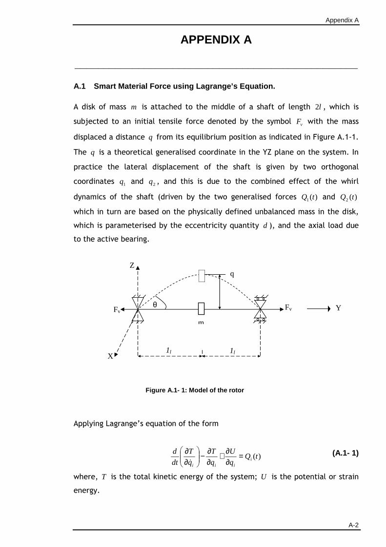
Appendix A
A-2
APPENDIX A
_________________________________________________
A.1 Smart Material Force using Lagrange’s Equation.
A disk of mass m is attached to the middle of a shaft of length l2 , which is
subjected to an initial tensile force denoted by the symbol vF with the mass
displaced a distance q from its equilibrium position as indicated in Figure A.1-1.
The q is a theoretical generalised coordinate in the YZ plane on the system. In
practice the lateral displacement of the shaft is given by two orthogonal
coordinates 1q and 2q , and this is due to the combined effect of the whirl
dynamics of the shaft (driven by the two generalised forces )(1 tQ and )(2 tQ
which in turn are based on the physically defined unbalanced mass in the disk,
which is parameterised by the eccentricity quantity d ), and the axial load due
to the active bearing.
Figure A.1- 1: Model of the rotor
Applying Lagrange’s equation of the form
)(tQ
q
U
q
T
q
T
dt
di
iii
=∂∂+
∂∂−
∂∂ɺ
(A.1- 1)
where, T is the total kinetic energy of the system; U is the potential or strain
energy.
1l 1l
Fv
m
q
θ Fv
Z
Y
X
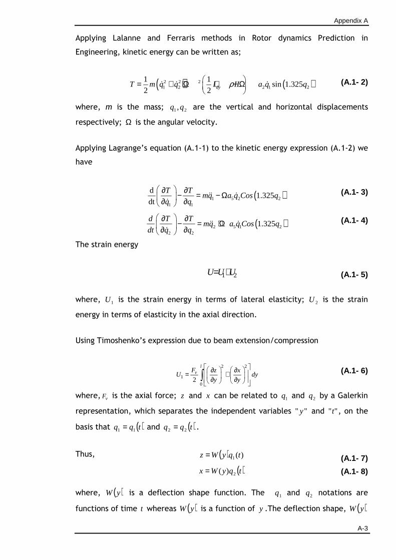
Appendix A
A-3
Applying Lalanne and Ferraris methods in Rotor dynamics Prediction in
Engineering, kinetic energy can be written as;
( ) ( )2 2 21 2 2 1 2
1 1sin 1.325
2 2 dyT m q q I IL a q qρ = + + Ω + − Ω
ɺ ɺ ɺ (A.1- 2)
where, m is the mass; 21,qq are the vertical and horizontal displacements
respectively; Ω is the angular velocity.
Applying Lagrange’s equation (A.1-1) to the kinetic energy expression (A.1-2) we
have
( )1 5 2 2
1 1
d1.325
dt
T Tmq a q Cos q
q q
∂ ∂− = − Ω ∂ ∂ ɺɺ ɺ
ɺ (A.1- 3)
( )2 5 1 2
2 2
1.325d T T
mq a q Cos qdt q q
∂ ∂− = + Ω ∂ ∂ ɺɺ ɺ
ɺ (A.1- 4)
The strain energy
1 2U U U= + (A.1- 5)
where, 1U is the strain energy in terms of lateral elasticity; 2U is the strain
energy in terms of elasticity in the axial direction.
Using Timoshenko’s expression due to beam extension/compression
2 2
1
02
lvF z x
U dyy y
∂ ∂ = + ∂ ∂ ∫ (A.1- 6)
where, vF is the axial force; z and x can be related to 1q and 2q by a Galerkin
representation, which separates the independent variables " "y and "" t , on the
basis that ( )tqq 11 = and ( )tqq 22 = .
Thus, ( ) )(1 tqyWz =
( )tqyWx 2)(=
(A.1- 7)
(A.1- 8)
where, ( )yW is a deflection shape function. The 1q and 2q notations are
functions of time t whereas ( )yW is a function of y .The deflection shape, ( )yW
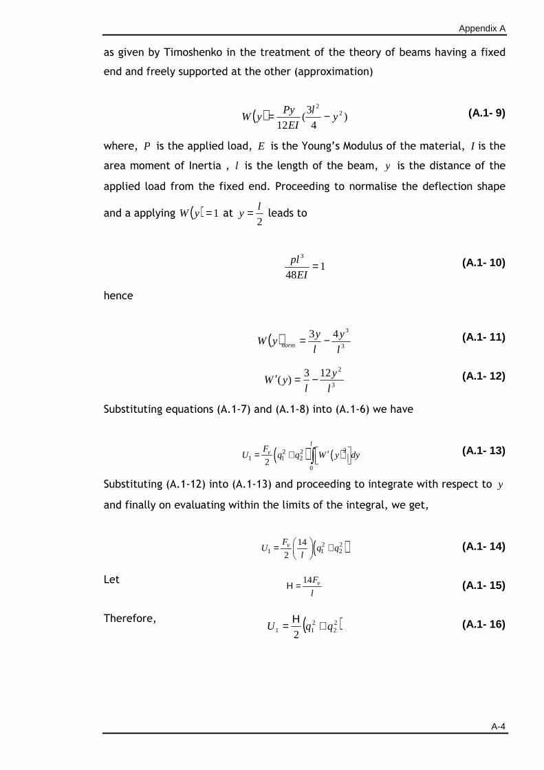
Appendix A
A-4
as given by Timoshenko in the treatment of the theory of beams having a fixed
end and freely supported at the other (approximation)
( ) )4
3(
122
2
yl
EI
PyyW −= (A.1- 9)
where, P is the applied load, E is the Young’s Modulus of the material, I is the
area moment of Inertia , l is the length of the beam, y is the distance of the
applied load from the fixed end. Proceeding to normalise the deflection shape
and a applying ( ) 1=yW at 2
ly = leads to
1
48
3
=EI
pl (A.1- 10)
hence
( )3
343
l
y
l
yyW norm −= (A.1- 11)
3
2123)(
l
y
lyW −=′ (A.1- 12)
Substituting equations (A.1-7) and (A.1-8) into (A.1-6) we have
( ) ( )22 2
1 1 2
02
lvF
U q q W y dy ′= + ∫ (A.1- 13)
Substituting (A.1-12) into (A.1-13) and proceeding to integrate with respect to y
and finally on evaluating within the limits of the integral, we get,
( )2 21 1 2
14
2vF
U q ql
= +
(A.1- 14)
Let 14 vF
lΗ = (A.1- 15)
Therefore,
( )22
211 2
qqU +Η= (A.1- 16)
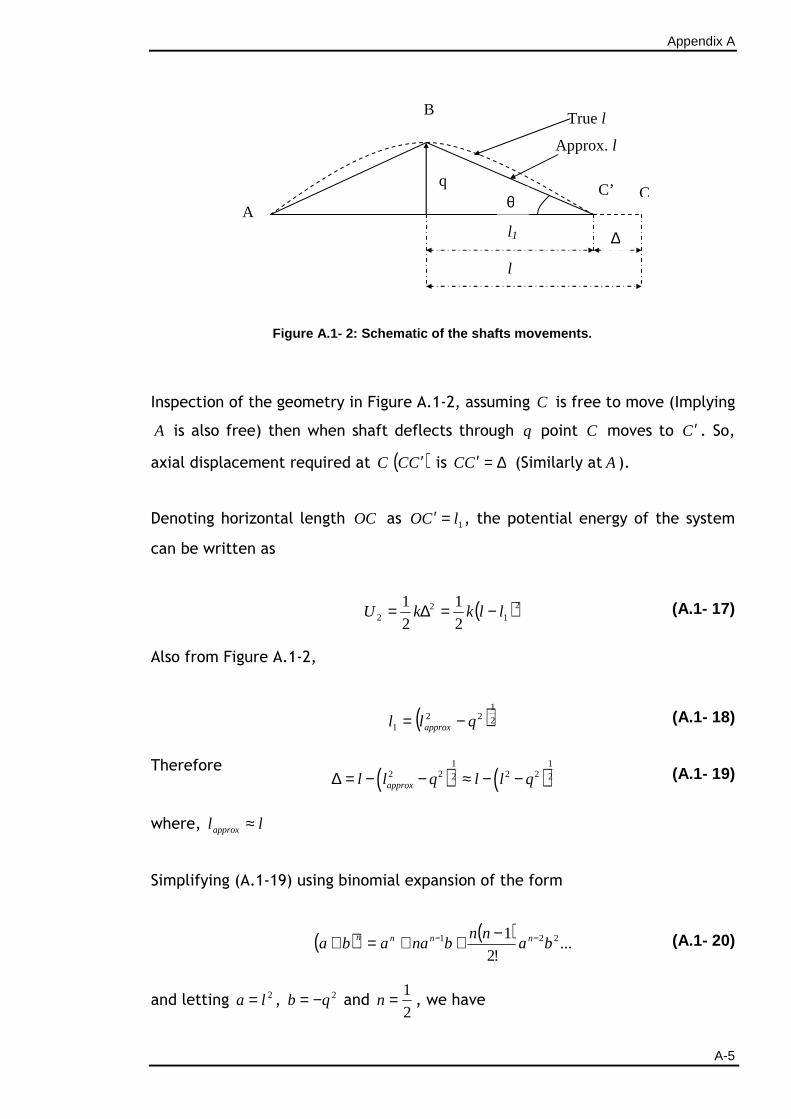
Appendix A
A-5
Figure A.1- 2: Sch ematic of the shafts movements.
Inspection of the geometry in Figure A.1-2, assuming C is free to move (Implying
A is also free) then when shaft deflects through q point C moves to C ′ . So,
axial displacement required at C ( )CC ′ is ∆=′CC (Similarly at A ).
Denoting horizontal length OC as 1lCO =′ , the potential energy of the system
can be written as
( )21
22 2
1
2
1llkkU −=∆= (A.1- 17)
Also from Figure A.1-2,
( )2
122
1 qll approx −= (A.1- 18)
Therefore ( ) ( )1 1
2 2 2 22 2approxl l q l l q∆ = − − ≈ − − (A.1- 19)
where, llapprox ≈
Simplifying (A.1-19) using binomial expansion of the form
( ) ( )...
!2
1 221 bann
bnaaba nnnn −− −++=+ (A.1- 20)
and letting 2la = , 2qb −= and 2
1=n , we have
A
C’
B
C
∆ l1
l
q θ
True l
Approx. l
Appendix A
A-6
( ) ( ) ( ) ( ) ( ) ( ) ...1*2
2
1
2
1
2
1 222
3222
122
1
2
122 2
+−
−
+−+=− −−qlqllql
l
ql
2
2
−≈
(A.1- 21)
Therefore ( )l
q
l
qllqll
22
22
2
122 ≈+−≈−− (A.1- 22)
Thus from equation (A.1-22) equation (A.1-19) may be replaced with a simpler
(but less accurate) equation by using the approximate relationship
l
q
2
2
≈∆ (A.1- 23)
Substituting equation(A.1-23) back into equation(A.1-17) we have,
22
2 22
1
=
l
qkU
(A.1- 24)
For a shaft of length l , axial force vF produces an extension ∆ . Force acts over
cross-sectional area A , producing normal stress
vF
Aσ = (A.1- 25)
The compression produces normal strain
l
∆=ε (A.1- 26)
Combining equations (A.1-25) and (A.1-26) yields relationship between force and
extension:
v
EAF k
l= ∆ = ∆ (A.1- 27)
where k is the shaft stiffness and l
EAk = . Substituting for k and considering
vertical and horizontal displacements (A.1-24) becomes
Appendix A
A-7
( )42
4132 8
qql
AEU += (A.1- 28)
Substituting equations (A.1-16) and (A.1-28) into equation (A.1-5) we get
( ) ( )42
413
22
21 82
qql
AEqqU +++Η= (A.1- 29)
Therefore,
3131
1 2q
l
AEq
q
U +Η=∂∂
(A.1- 30)
And
3232
2 2q
l
AEq
q
U +Η=∂∂
(A.1- 31)
Substituting equations (A.1-30), (A.1-31), (A.1-3) and (A.1-4) into equation
(A.1-1) we have
( ) ( )31 5 2 2 1 1 13
1.3252
AEmq a q Cos q q q Q t
l− Ω + Η + =ɺɺ ɺ (A.1- 32)
( ) ( )32 5 1 2 2 2 23
1.3252
AEmq a q Cos q q q Q t
l+ Ω + Η + =ɺɺ ɺ (A.1- 33)
Substituting equation (A.1-15) into equations (A.1-32) and (A.1-33) gives
( ) ( )31 5 2 2 1 1 13
141.325
2vF AE
mq a q Cos q q q Q tl l
− Ω + + =ɺɺ ɺ (A.1- 34)
( ) ( )32 5 1 2 2 2 23
141.325
2vF AE
mq a q Cos q q q Q tl l
+ Ω + + =ɺɺ ɺ (A.1- 35)
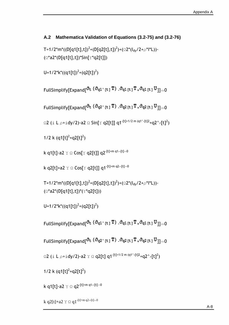
Appendix A
A-8
A.2 Mathematica Validation of Equations (3.2-75) an d (3.2-76)
T=1/2*m*((D[q1[t],t])2+(D[q2[t],t])2)+(Ω2*(Idy/2+ρ*I*L))-
(Ω*a2*(D[q1[t],t])*Sin[Υ*q2[t]])
U=1/2*k*((q1[t])2+(q2[t])2)
FullSimplify[Expand[∂t H∂q1' @t DTL-∂q1@t DT+∂q1@t DU]]0
FullSimplify[Expand[∂t H∂q2' @t DTL-∂q2@t DT+∂q2@t DU]]0
Ω2 ( L ρ+dy/2)-a2 Ω Sin[Υ q2[t]] q1′[t]+1/2 m (q1^′[t]2+q2^′[t]2)
1/2 k (q1[t]2+q2[t]2)
k q1[t]-a2 Υ Ω Cos[Υ q2[t]] q2′[t]+m q1′′[t]0
k q2[t]+a2 Υ Ω Cos[Υ q2[t]] q1′[t]+m q2′′[t]0
T=1/2*m*((D[q1[t],t])2+(D[q2[t],t])2)+(Ω2*(Idy/2+ρ*I*L))-
(Ω*a2*(D[q1[t],t])*(Υ*q2[t]))
U=1/2*k*((q1[t])2+(q2[t])2)
FullSimplify[Expand[∂t H∂q1' @t DTL-∂q1@t DT+∂q1@t DU]]0
FullSimplify[Expand[∂t H∂q2' @t DTL-∂q2@t DT+∂q2@t DU]]0
Ω2 ( L ρ+dy/2)-a2 Υ Ω q2[t] q1′[t]+1/2 m (q1^′[t]2+q2^′[t]2)
1/2 k (q1[t]2+q2[t]2)
k q1[t]-a2 Υ Ω q2′[t]+m q1′′[t]0
k q2[t]+a2 Υ Ω q1′[t]+m q2′′[t]0
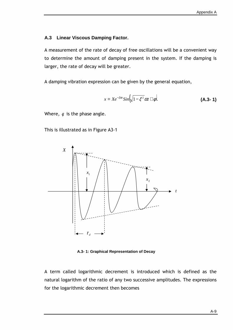
Appendix A
A-9
A.3 Linear Viscous Damping Factor.
A measurement of the rate of decay of free oscillations will be a convenient way
to determine the amount of damping present in the system. If the damping is
larger, the rate of decay will be greater.
A damping vibration expression can be given by the general equation,
( )φωξξω +−= − tSinXex t 21 (A.3- 1)
Where, φ is the phase angle.
This is illustrated as in Figure A3-1
A.3- 1: Graphical Rep resentation of Decay
A term called logarithmic decrement is introduced which is defined as the
natural logarithm of the ratio of any two successive amplitudes. The expressions
for the logarithmic decrement then becomes
X
t
1x
2x
dτ
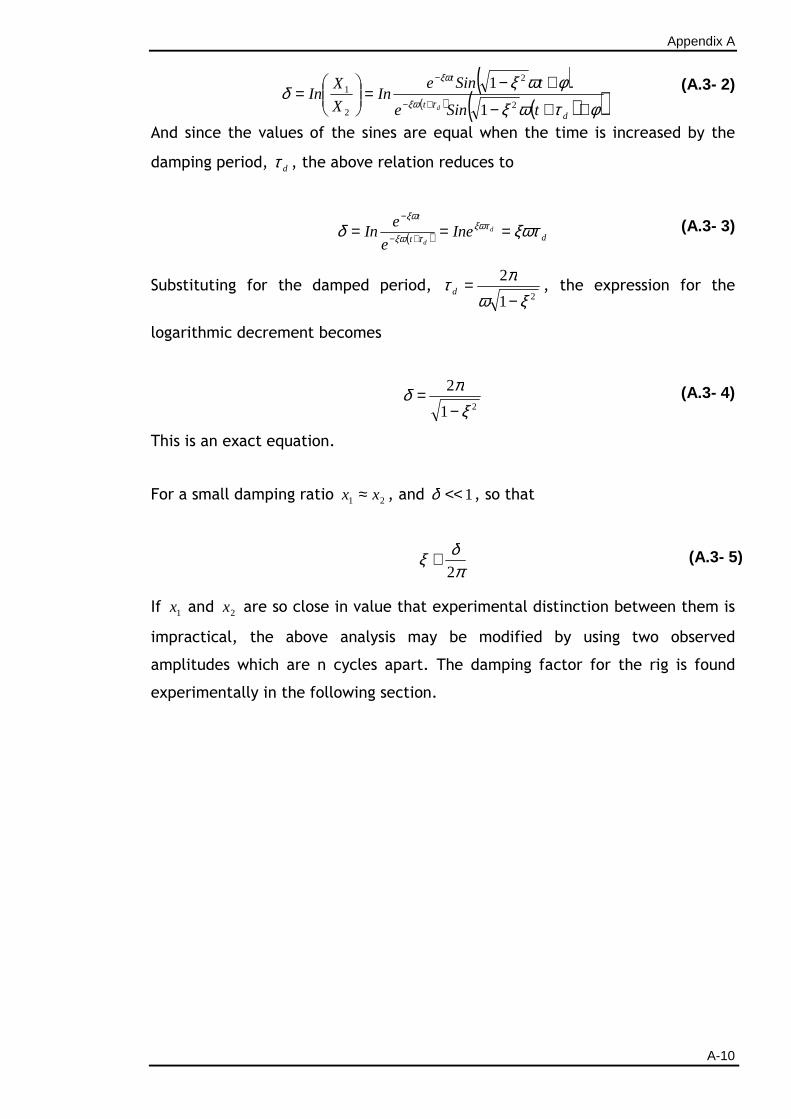
Appendix A
A-10
( )( ) ( )( )φτωξ
φωξδ
τξω
ξω
++−
+−=
=
+−
−
dt
t
tSine
tSineIn
X
XIn
d 2
2
2
1
1
1
(A.3- 2)
And since the values of the sines are equal when the time is increased by the
damping period, dτ , the above relation reduces to
( ) dt
td
dIne
e
eIn ξωτδ ξωτ
τξω
ξω
=== +−
−
(A.3- 3)
Substituting for the damped period, 21
2
ξωπτ−
=d , the expression for the
logarithmic decrement becomes
21
2
ξπδ−
= (A.3- 4)
This is an exact equation.
For a small damping ratio 21 xx ≈ , and 1<<δ , so that
πδξ2
≅ (A.3- 5)
If 1x and 2x are so close in value that experimental distinction between them is
impractical, the above analysis may be modified by using two observed
amplitudes which are n cycles apart. The damping factor for the rig is found
experimentally in the following section.
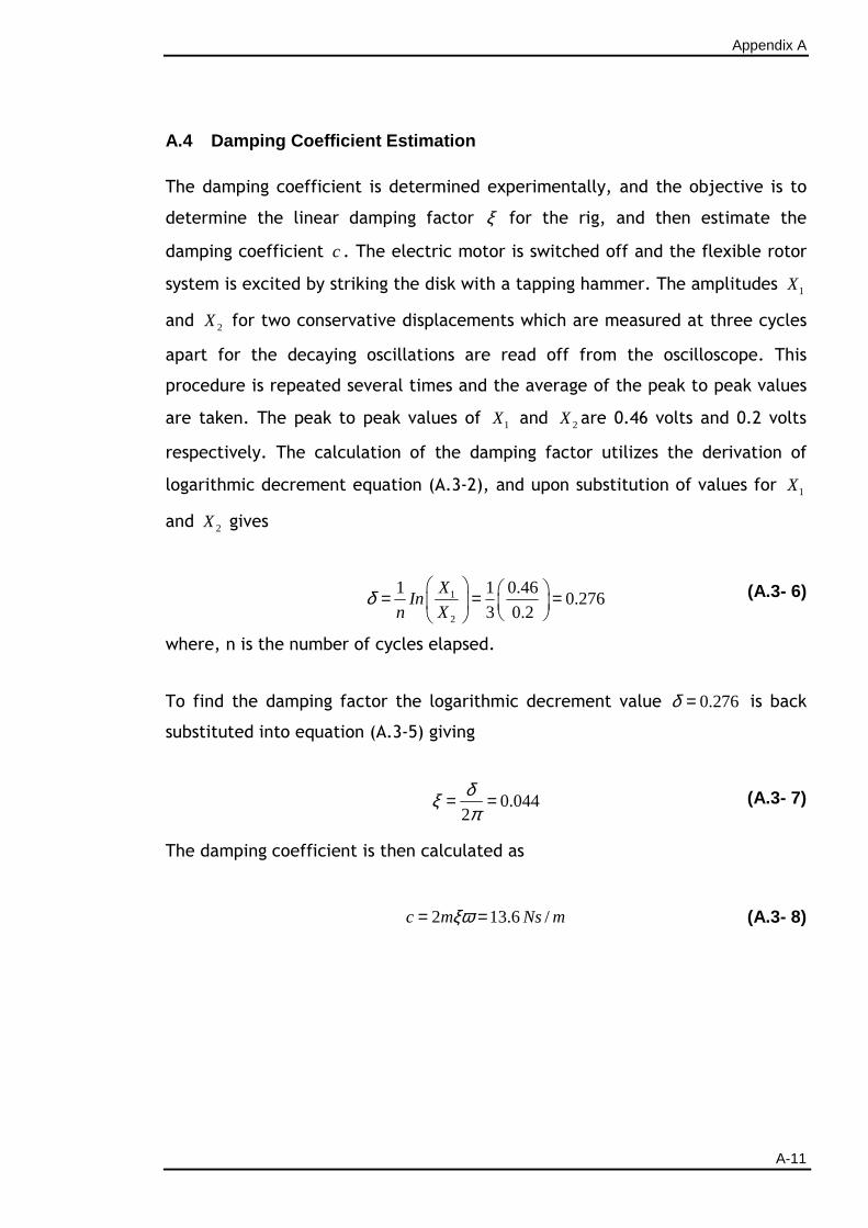
Appendix A
A-11
A.4 Damping Coefficient Estimation
The damping coefficient is determined experimentally, and the objective is to
determine the linear damping factor ξ for the rig, and then estimate the
damping coefficient c . The electric motor is switched off and the flexible rotor
system is excited by striking the disk with a tapping hammer. The amplitudes 1X
and 2X for two conservative displacements which are measured at three cycles
apart for the decaying oscillations are read off from the oscilloscope. This
procedure is repeated several times and the average of the peak to peak values
are taken. The peak to peak values of 1X and 2X are 0.46 volts and 0.2 volts
respectively. The calculation of the damping factor utilizes the derivation of
logarithmic decrement equation (A.3-2), and upon substitution of values for 1X
and 2X gives
1
2
1 1 0.460.276
3 0.2
XIn
n Xδ
= = =
(A.3- 6)
where, n is the number of cycles elapsed.
To find the damping factor the logarithmic decrement value 0.276δ = is back
substituted into equation (A.3-5) giving
0.044
2
δξπ
= = (A.3- 7)
The damping coefficient is then calculated as
2 13.6 /c m Ns mξω= = (A.3- 8)
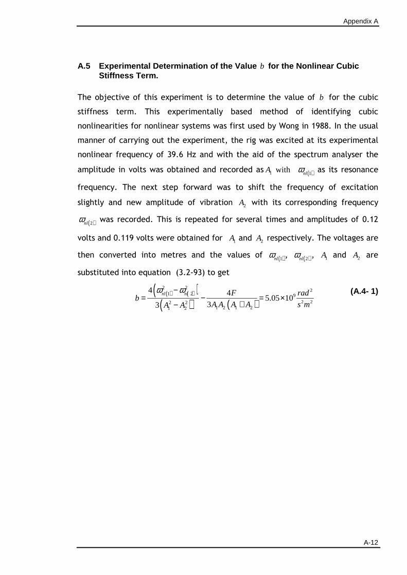
Appendix A
A-12
A.5 Experimental Determination of the Value b for the Nonlinear Cubic Stiffness Term.
The objective of this experiment is to determine the value of b for the cubic
stiffness term. This experimentally based method of identifying cubic
nonlinearities for nonlinear systems was first used by Wong in 1988. In the usual
manner of carrying out the experiment, the rig was excited at its experimental
nonlinear frequency of 39.6 Hz and with the aid of the spectrum analyser the
amplitude in volts was obtained and recorded as 1A with ( )1nlω as its resonance
frequency. The next step forward was to shift the frequency of excitation
slightly and new amplitude of vibration 2A with its corresponding frequency
( )2nlω was recorded. This is repeated for several times and amplitudes of 0.12
volts and 0.119 volts were obtained for 1A and 2A respectively. The voltages are
then converted into metres and the values of ( )1nlω , ( )2nlω , 1A and 2A are
substituted into equation (3.2-93) to get
( ) ( )( )
( ) ( )
2 22
1 2 92 22 2
1 2 1 21 2
4 45.05 10
33
nl nl F radb
A A A A s mA A
ω ω−= − = ×
+−
(A.4- 1)
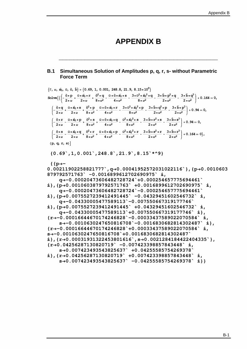
Appendix B
B-1
APPENDIX B
___________________________________________
B.1 Simultaneous Solution of Amplitudes p, q, r, s- without Parametric Force Term
9Γ, ω, a 5ˆ , Ω, cˆ, b
ˆ= = 90.69, 1, 0.001, 248.8, 21.9, 8.15 ∗109=
Solve A9i
k
jjjj−cˆ∗p
2∗ ω+
Ω∗a5ˆ∗r
2∗ω+
cˆ2∗q
8∗ω2−
Ω ∗cˆ∗a5ˆ∗s
4∗ω2−
3∗Ω2∗a5ˆ 2∗q
8∗ω2−
3∗bˆ∗p2∗q
2∗ω2−
3∗bˆ∗q3
2∗ω2
y
zzzz+0.164 0,
i
k
jjjj−cˆ∗q
2∗ω+
Ω∗a5ˆ∗s
2∗ω+
cˆ2∗ p
8∗ ω2−
Ω ∗cˆ∗a5ˆ∗r
4∗ω2−
3∗Ω2∗a5ˆ 2∗p
8∗ω2−
3∗bˆ∗q2∗p
2∗ω2−
3∗bˆ∗p3
2∗ω2
y
zzzz+0.94 0,
i
k
jjjj−cˆ∗r
2∗ω−
Ω∗a5ˆ∗p
2∗ ω+
cˆ2∗ s
8∗ω2+
Ω ∗cˆ∗a5ˆ∗q
4∗ω2−
Ω2∗a5ˆ 2∗ s
8∗ω2−
3∗bˆ∗r 2∗s
2∗ω2−
3∗bˆ∗s3
2∗ω2
y
zzzz +0.94 0,
i
k
jjjj−cˆ∗s
2∗ω−
Ω∗a5ˆ∗q
2∗ω+
cˆ2∗ r
8∗ω2+
Ω ∗cˆ∗a5ˆ∗p
4∗ω2−
Ω2∗a5ˆ 2∗ r
8∗ω2−
3∗bˆ∗s2∗r
2∗ω2−
3∗bˆ∗r 3
2∗ω2
y
zzzz +0.164 0=,
8p, q, r, s <E 0.69`,1,0.001`,248.8`,21.9`,8.15`*^9 p →-0.00211902258821777`,q →0.00041952572031022116`,p →0.0010603879792571763` -0.0016899612702690975` , q →-0.00020473606482728724`+0.000254657775694461` ,p →0.0010603879792571763` +0.0016899612702690975` , q →-0.00020473606482728724`-0.000254657775694461` ,p →0.0075527239412491445` -0.04329451602546732` , q →-0.04330005477589113`-0.007550667319177746` ,p →0.0075527239412491445` +0.04329451602546732` , q →-0.04330005477589113`+0.007550667319177746` , r →-0.00016644670174246828`-0.00033437589022070584` , s →-0.0010630247650816708`-0.0016830682814302487` , r →-0.00016644670174246828`+0.00033437589022070584` , s→-0.0010630247650816708`+0.0016830682814302487` ,r →0.00031931322453801616`,s →0.0021284184422404335`, r →0.04256287130820719` -0.007423398857843448` , s →0.007423493543825637` +0.04255585754269378` ,r →0.04256287130820719` +0.007423398857843448` , s →0.007423493543825637` -0.04255585754269378`
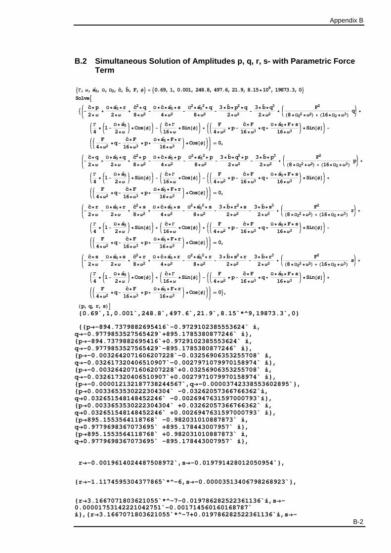
Appendix B
B-2
B.2 Simultaneous Solution of Amplitudes p, q, r, s- with Parametric Force Term
9Γ, ω, a 5ˆ , Ω, Ω2, cˆ, b
ˆ, F, φ= =90.69, 1, 0.001, 248.8, 497.6, 21.9, 8.15 ∗109, 19873.3, 0 =
Solve A
9i
k
jjjj−cˆ∗ p
2∗ ω+
Ω∗a5ˆ∗r
2∗ω+
cˆ2∗q
8∗ω2−
Ω∗cˆ∗a5ˆ∗s
4∗ω2−
Ω2∗a5ˆ 2∗q
8∗ω2−
3∗bˆ∗p2∗q
2∗ω2−
3∗ bˆ∗q3
2∗ω2+ikjj F2
H8∗Ω22∗ω2L +H16∗Ω2∗ω3L qyzz +
ikjjΓ
4∗ikjj1−
Ω∗a5ˆ
2∗ωyzz∗Cos@φDy
zz −
ikjj
cˆ∗Γ
16∗ω∗Sin @φDy
zz +
ikjjikjj
F
4∗ω2∗p−
cˆ∗F
16 ∗ω3∗q+
Ω∗a5ˆ∗F∗ s
16∗ω3
yzz∗Sin @φDy
zz −
ikjjikjj
F
4∗ω2∗q−
cˆ∗F
16∗ω3∗p+
Ω∗a5ˆ∗F∗ r
16∗ω3
yzz∗Cos@φDy
zzy
zzzz 0,
i
k
jjjj−cˆ∗q
2∗ω+
Ω∗a5ˆ∗q
2∗ω+
cˆ2∗ p
8∗ω2−
Ω∗cˆ∗a5ˆ∗ p
4∗ω2−
Ω2∗a5ˆ 2∗ p
8∗ω2−
3∗bˆ∗q2∗p
2∗ω2−
3∗bˆ∗p3
2∗ω2+ikjj F2
H8∗Ω22∗ω2L +H16∗Ω2∗ω3L pyzz +
ikjjΓ
4∗ikjj1−
Ω∗a5ˆ
2∗ωyzz∗Sin @φDy
zz −
ikjj
cˆ∗Γ
16∗ω∗Cos@φDy
zz −
ikjjikjj
F
4∗ω2∗p−
cˆ∗F
16 ∗ω3∗q+
Ω∗a5ˆ∗F∗ s
16∗ω3
yzz∗Sin @φDy
zz +
ikjjikjj
F
4∗ω2∗q−
cˆ∗F
16∗ω3∗p+
Ω∗a5ˆ∗F∗ r
16∗ω3
yzz∗Cos@φDy
zzy
zzzz 0,
i
k
jjjj−cˆ∗ r
2∗ω−
Ω∗a5ˆ∗r
2∗ω+
cˆ2∗ s
8∗ω2+
Ω∗cˆ∗a5ˆ∗s
4∗ω2−
Ω2∗a5ˆ 2∗ s
8∗ω2−
3∗bˆ∗r 2∗s
2∗ω2−
3∗ bˆ∗s3
2∗ω2+ikjj F2
H8∗Ω22∗ω2L +H16∗Ω2∗ω3L ryzz +
ikjjΓ
4∗ikjj1−
Ω∗a5ˆ
2∗ωyzz∗Sin @φDy
zz +
ikjj
cˆ∗Γ
16∗ω∗Cos@φDy
zz +
ikjjikjj
F
4∗ω2∗p−
cˆ∗F
16 ∗ω3∗q+
Ω∗a5ˆ∗F∗ s
16∗ω3
yzz∗Sin @φDy
zz −
ikjjikjj
F
4∗ω2∗q−
cˆ∗F
16∗ω3∗p+
Ω∗a5ˆ∗F∗ r
16∗ω3
yzz∗Cos@φDy
zzy
zzzz 0,
i
k
jjjj−cˆ∗s
2∗ω−
Ω∗a5ˆ∗s
2∗ω+
cˆ2∗ r
8∗ω2+
Ω∗cˆ∗a5ˆ∗ r
4∗ω2−
Ω2∗a5ˆ 2∗ r
8∗ω2−
3∗bˆ∗s2∗r
2∗ω2−
3∗ bˆ∗r 3
2∗ω2+ikjj F2
H8∗Ω22∗ω2L +H16∗Ω2∗ω3L syzz +
ikjjΓ
4∗ikjj1−
Ω∗a5ˆ
2∗ωyzz∗Cos@φDy
zz +
ikjj
cˆ∗Γ
16∗ω∗Sin @φDy
zz −
ikjjikjj
F
4∗ω2∗p−
cˆ∗F
16 ∗ω3∗q+
Ω∗a5ˆ∗F∗ s
16∗ω3
yzz∗Sin @φDy
zz +
ikjjikjj
F
4∗ω2∗q−
cˆ∗F
16∗ω3∗p+
Ω∗a5ˆ∗F∗ r
16∗ω3
yzz∗Cos@φDy
zzy
zzzz 0=,
8p, q, r, s <E 0.69`,1,0.001`,248.8`,497.6`,21.9`,8.15`*^9,19873 .3`,0 p →-894.7379882695416`-0.9729102385553624` , q→-0.9779853527565429`+895.1785380877246` , p →-894.7379882695416`+0.9729102385553624` , q→-0.9779853527565429`-895.1785380877246` , p →-0.0032642071606207228`-0.03256906353255708` , q→-0.032617320406510907`-0.0027971079970158974` , p →-0.0032642071606207228`+0.03256906353255708` , q→-0.032617320406510907`+0.0027971079970158974` , p →-0.000012132187738244567`,q →-0.00003742338553602895`, p →0.0033653530222304304` -0.03262057366766362` , q→0.032651548148452246` -0.0026947631597000793` , p →0.0033653530222304304` +0.03262057366766362` , q→0.032651548148452246` +0.0026947631597000793` , p →895.1553564118768` -0.982031010887873` , q→0.9779698367073695` +895.178443007957` , p →895.1553564118768` +0.982031010887873` , q→0.9779698367073695` -895.178443007957` ,
r →-0.0019614024487508972`,s →-0.019791428012050954`,
r →-1.1174595304377865`*^-6,s →-0.00003513406798268923`,
r →3.1667071803621055`*^-7-0.019786282522361136` ,s →-0.00001753142221042751`-0.001714560160168787` ,r →3.1667071803621055`*^-7+0.019786282522361136` ,s →-
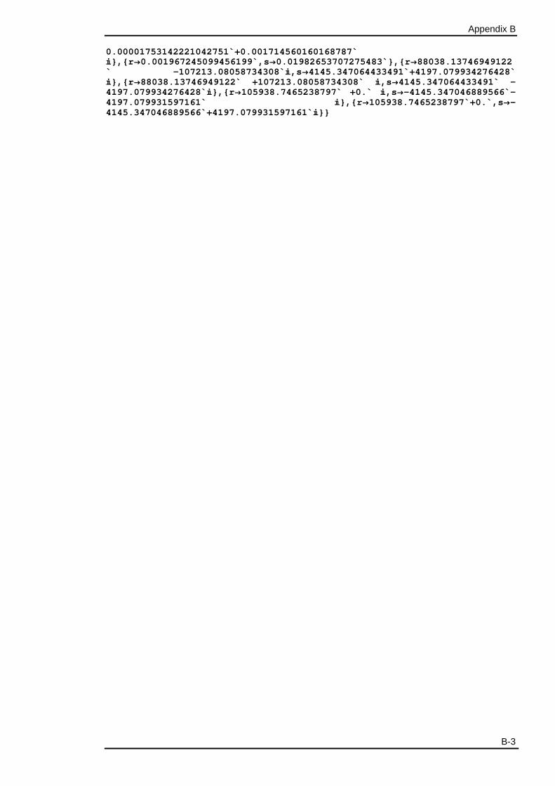
Appendix B
B-3
0.00001753142221042751`+0.001714560160168787` ,r →0.001967245099456199`,s →0.01982653707275483`,r →88038.13746949122` -107213.08058734308` ,s →4145.347064433491`+4197.079934276428` ,r →88038.13746949122` +107213.08058734308` ,s →4145.347064433491` -4197.079934276428` ,r →105938.7465238797` +0.` ,s →-4145.347046889566`-4197.079931597161` ,r →105938.7465238797`+0.`,s →-4145.347046889566`+4197.079931597161`
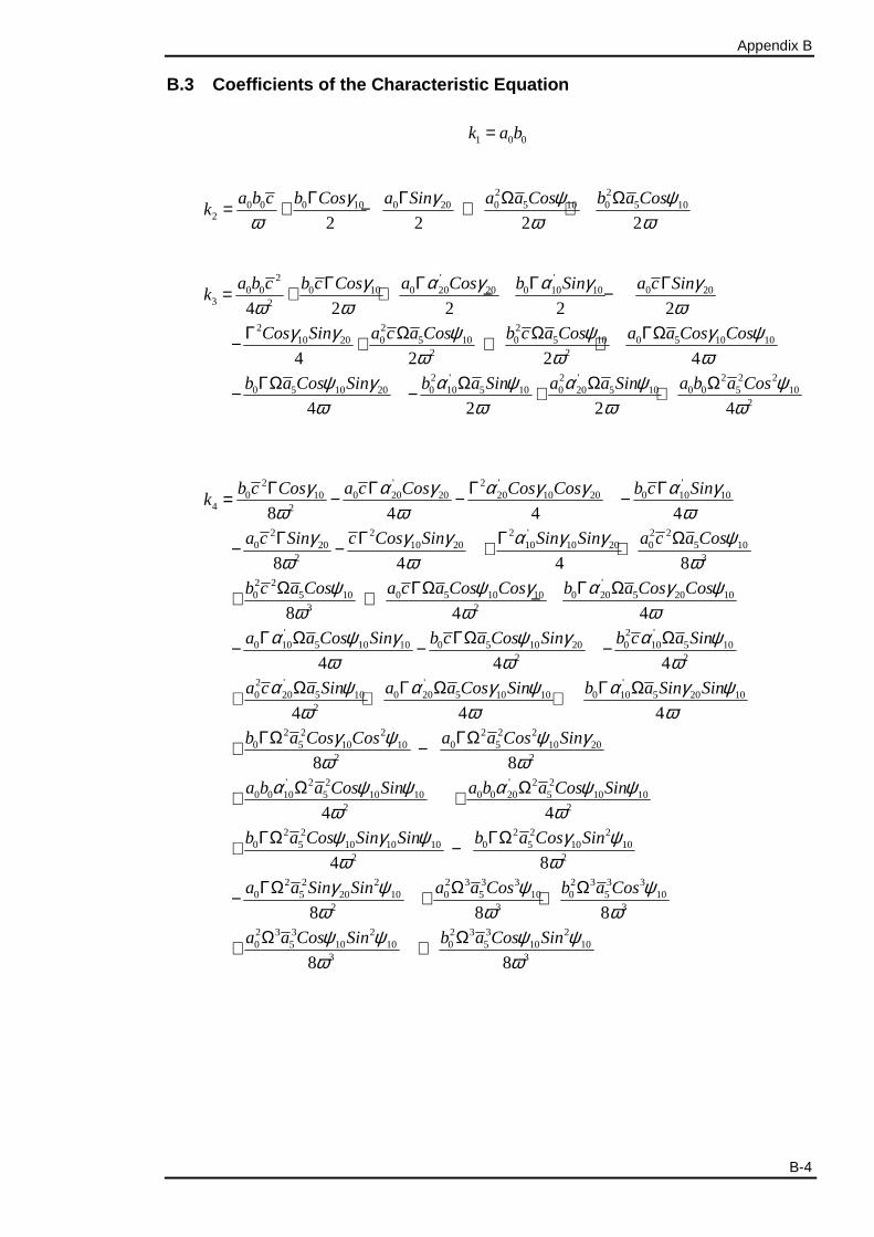
Appendix B
B-4
B.3 Coefficients of the Characteristic Equation
1 0 0k a b=
2 20 0 0 10 0 20 0 5 10 0 5 10
2 2 2 2 2
a b c b Cos a Sin a a Cos b a Cosk
γ γ ψ ψω ω ω
Γ Γ Ω Ω= + − + +
2 ' '0 0 0 10 0 20 20 0 10 10 0 20
3 2
2 2 210 20 0 5 10 0 5 10 0 5 10 10
2 2
2 ' 2 '0 5 10 20 0 10 5 10 0 20 5 10
4 2 2 2 2
4 2 2 4
4 2 2
a b c b c Cos a Cos b Sin a c Sink
Cos Sin a c a Cos b c a Cos a a Cos Cos
b a Cos Sin b a Sin a a Sin a
γ α γ α γ γω ω ω
γ γ ψ ψ γ ψω ω ω
ψ γ α ψ α ψω ω ω
Γ Γ Γ Γ= + + − −
Γ Ω Ω ΓΩ− + + +
ΓΩ Ω Ω− − + +2 2 2
0 0 5 1024
b a Cos ψω
Ω
2 ' 2 ' '0 10 0 20 20 20 10 20 0 10 10
4 2
2 2 2 ' 2 20 20 10 20 10 10 20 0 5 10
2 3
2 2 '0 5 10 0 5 10 10 0 20 5 20
3 2
8 4 4 4
8 4 4 8
8 4
b c Cos a c Cos Cos Cos b c Sink
a c Sin c Cos Sin Sin Sin a c a Cos
b c a Cos a c a Cos Cos b a Cos
γ α γ α γ γ α γω ω ω
γ γ γ α γ γ ψω ω ω
ψ ψ γ α γω ω
Γ Γ Γ Γ= − − −
Γ Γ Γ Ω− − + +
Ω ΓΩ Γ Ω+ + − 10
' 2 '0 10 5 10 10 0 5 10 20 0 10 5 10
2 2
2 ' ' '0 20 5 10 0 20 5 10 10 0 10 5 20 10
2
2 2 2 2 2 20 5 10 10 0 5 10 20
2 2
4
4 4 4
4 4 4
8 8
Cos
a a Cos Sin b c a Cos Sin b c a Sin
a c a Sin a a Cos Sin b a Sin Sin
b a Cos Cos a a Cos Sin
a
ψω
α ψ γ ψ γ α ψω ω ω
α ψ α γ ψ α γ ψω ω ω
γ ψ ψ γω ω
Γ Ω ΓΩ Ω− − −
Ω Γ Ω Γ Ω+ + +
ΓΩ ΓΩ+ −
+' 2 2 ' 2 2
0 0 10 5 10 10 0 0 20 5 10 102 2
2 2 2 2 20 5 10 10 10 0 5 10 10
2 2
2 2 2 2 3 3 3 2 3 3 30 5 20 10 0 5 10 0 5 10
2 3 3
2 3 3 20 5 10 10
3
4 4
4 8
8 8 8
8
b a Cos Sin a b a Cos Sin
b a Cos Sin Sin b a Cos Sin
a a Sin Sin a a Cos b a Cos
a a Cos Sin
α ψ ψ α ψ ψω ωψ γ ψ γ ψω ω
γ ψ ψ ψω ω ωψ ψ
ω
Ω Ω+
ΓΩ ΓΩ+ −
ΓΩ Ω Ω− + +
Ω+ +2 3 3 20 5 10 10
38
b a Cos Sinψ ψω
Ω
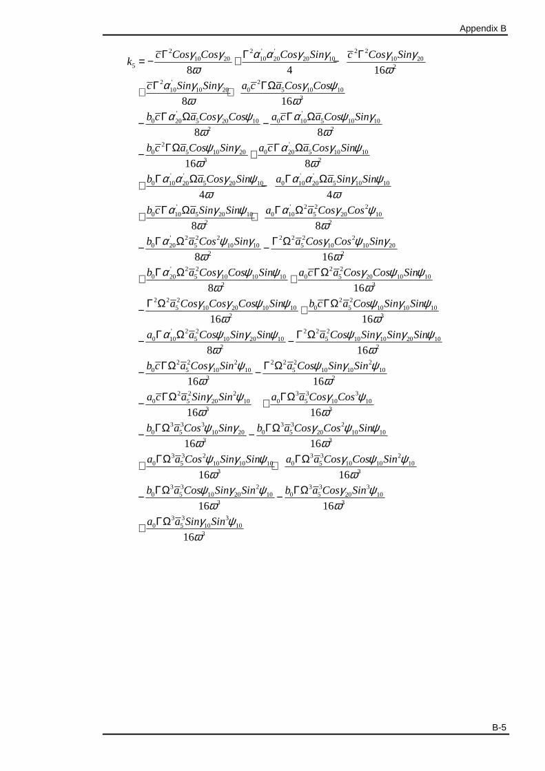
Appendix B
B-5
2 2 ' ' 2 210 20 10 20 20 10 10 20
5 2
2 ' 210 10 20 0 5 10 10
3
' '0 20 5 20 10 0 10 5 10 10
2 2
20 5 10 20 0 20
3
8 4 16
8 16
8 8
16
c Cos Cos Cos Sin c Cos Sink
c Sin Sin a c a Cos Cos
b c a Cos Cos a c a Cos Sin
b c a Cos Sin a c
γ γ α α γ γ γ γω ω
α γ γ γ ψω ω
α γ ψ α ψ γω ωψ γ α
ω
Γ Γ Γ= − + −
Γ ΓΩ+ +
Γ Ω Γ Ω− −
ΓΩ Γ− +'
5 10 102
' ' ' '0 10 20 5 20 10 0 10 20 5 10 10
' ' 2 2 20 10 5 20 10 0 10 5 20 10
2 2
' 2 2 2 2 2 2 20 20 5 10 10 5 10 10 20
2 2
0 20
8
4 4
8 8
8 16
a Cos Sin
b a Cos Sin a a Sin Sin
b c a Sin Sin a a Cos Cos
b a Cos Sin a Cos Cos Sin
b
γ ψω
α α γ ψ α α γ ψω ω
α γ ψ α γ ψω ω
α ψ γ γ ψ γω ω
α
Ω
Γ Ω Γ Ω+ −
Γ Ω Γ Ω+ +
Γ Ω Γ Ω− −
Γ+' 2 2 2 2
5 10 10 10 0 5 20 10 102 3
2 2 2 2 25 10 20 10 10 0 5 10 10 10
2 3
' 2 2 2 2 20 10 5 10 20 10 5 10 10 20 10
2 2
0
8 16
16 16
8 16
a Cos Cos Sin a c a Cos Cos Sin
a Cos Cos Cos Sin b c a Cos Sin Sin
a a Cos Sin Sin a Cos Sin Sin Sin
b
γ ψ ψ γ ψ ψω ω
γ γ ψ ψ ψ γ ψω ω
α ψ γ ψ ψ γ γ ψω ω
Ω ΓΩ+
Γ Ω ΓΩ− +
Γ Ω Γ Ω− −
−2 2 2 2 2 2 2
5 10 10 5 10 10 103 2
2 2 2 3 3 30 5 20 10 0 5 10 10
3 3
3 3 3 3 3 20 5 10 20 0 5 20 10 10
3 3
3 3 20 5 10 10 10
3
16 16
16 16
16 16
16
c a Cos Sin a Cos Sin Sin
a c a Sin Sin a a Cos Cos
b a Cos Sin b a Cos Cos Sin
a a Cos Sin Sin a
γ ψ ψ γ ψω ω
γ ψ γ ψω ω
ψ γ γ ψ ψω ω
ψ γ ψω
ΓΩ Γ Ω−
ΓΩ ΓΩ− +
ΓΩ ΓΩ− −
ΓΩ+ +3 3 2
0 5 10 10 103
3 3 2 3 3 30 5 10 20 10 0 5 20 10
3 3
3 3 30 5 10 10
3
16
16 16
16
a Cos Cos Sin
b a Cos Sin Sin b a Cos Sin
a a Sin Sin
γ ψ ψω
ψ γ ψ γ ψω ω
γ ψω
ΓΩ
ΓΩ ΓΩ− −
ΓΩ+
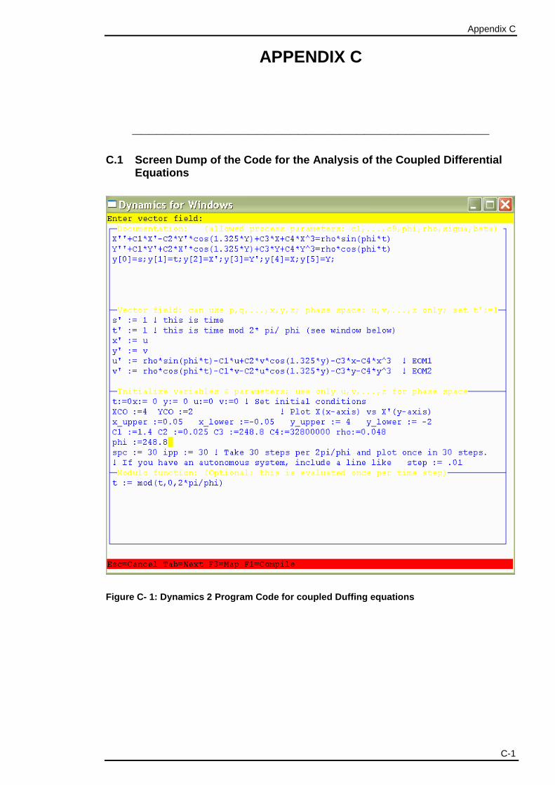
Appendix C
C-1
APPENDIX C
___________________________________________
C.1 Screen Dump of the Code for the Analysis of the Coupled Differential Equations
Figure C- 1: Dynamics 2 Program Code for coupled Du ffing equations

Appendix C
C-2
C.2 Specialized Code written in MathematicaTM
C.2.1 Numerical Integration
( )321 1 5 2 2 1 1
2
ˆˆ ˆ[ ] * [ ] * * [ ]*cos[ * [ ]] * [ ] * [ ]
* * *sin[ * ]
eqns q t c q t a q t q t q t b q t
d t
γ ω
µ
′′ ′ ′= + − Ω + +
− Ω Ω
( )322 2 5 1 2 2 2
2
ˆˆ ˆ[ ] * [ ] * * [ ]*cos[ * [ ]] * [ ] * [ ]
* * *cos[ * ]
eqnt q t c q t a q t q t q t b q t
d t
γ ω
µ
′′ ′ ′= + − Ω + +
− Ω Ω
system= NDSolve[eqns==0,eqnt==0, 1[0] 0q == , 2[0] 0q == , 1[0] 0q′ == ,
2[0] 0q′ == , 1q , 2q ,t,0,50,MaxSteps→ Infinity,AccuracyGoal→Automatic,
PrecisionGoal →Automatic, WorkingPrecision →20]
Plot[Evaluate[ 1q [t]/.system], t,0,50, Frame →True, FrameTicks→Automatic,
GridLines→Automatic, FrameLabel→ Time, 1q [t]]
Plot[Evaluate[ 1q′ [t]/.system], t,0,50, Frame →True, FrameTicks→Automatic,
GridLines→Automatic, FrameLabel→ Time, 1q′ [t]]
C.2.2 Plotting of Poincaré Map system=NDSolve[eqns==0,eqnt==0, [0] 0x == , [0] 0u == , [0] 0v == , x ,t,0,T,
Method→Runge-Kutta,
MaxSteps→ Infinity,AccuracyGoal→Automatic,PrecisionGoal→Automatic,
WorkingPrecision →20]
ParametricPlot[Evaluate[ x [t],u [t]/.system],t,0,T,PlotRange→All,
Frame →True, FrameLabel→ x [t], u [t]] Texternal=2 /π ω∗
ParametricPlot[Evaluate[ x [t], v [t]/.system],t,0,T,PlotRange→All,
Frame →True, FrameLabel→ x [t], v [t]] Texternal=2 /π ω∗
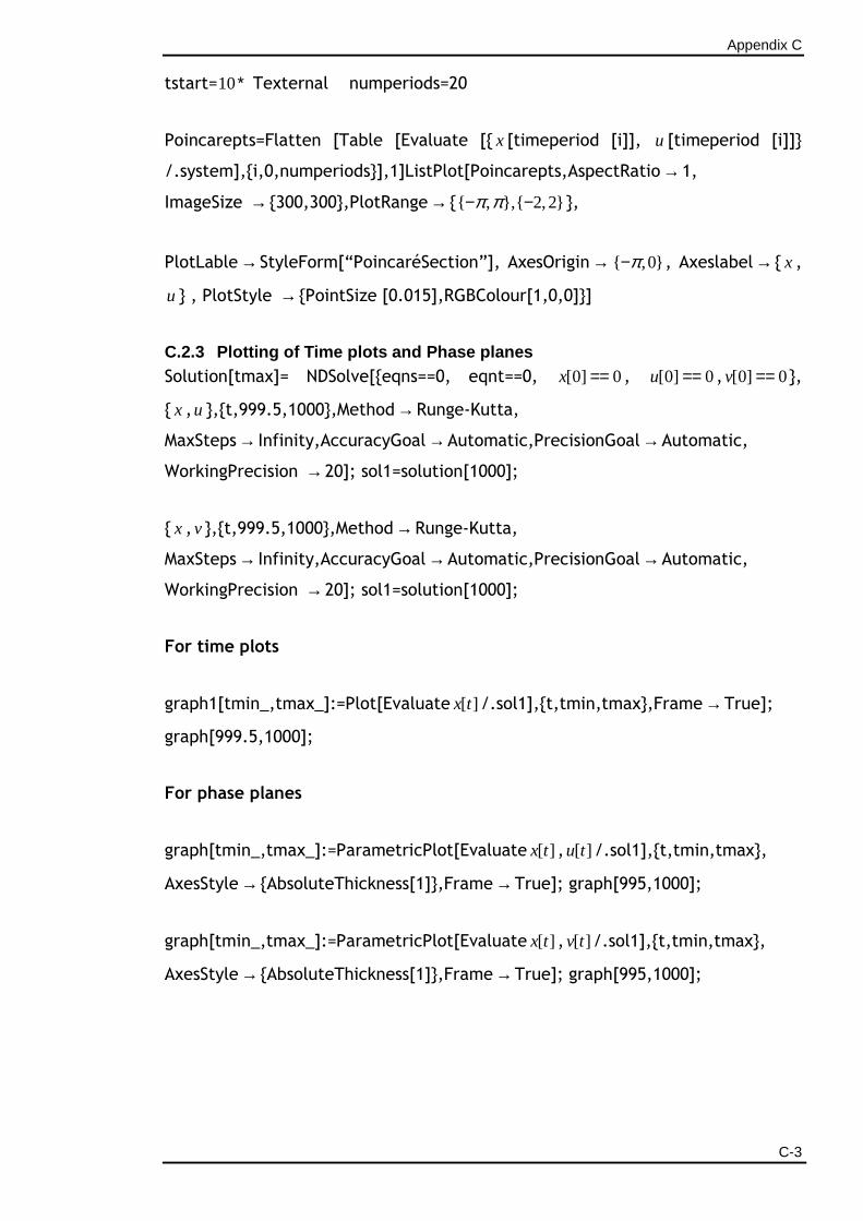
Appendix C
C-3
tstart=10∗ Texternal numperiods=20
Poincarepts=Flatten [Table [Evaluate [ x [timeperiod [i]], u [timeperiod [i]]
/.system],i,0,numperiods],1]ListPlot[Poincarepts,AspectRatio→1,
ImageSize → 300,300,PlotRange→ , , 2,2π π− − ,
PlotLable→StyleForm[“PoincaréSection”], AxesOrigin→ ,0π− , Axeslabel→ x ,
u , PlotStyle → PointSize [0.015],RGBColour[1,0,0]]
C.2.3 Plotting of Time plots and Phase planes Solution[tmax]= NDSolve[eqns==0, eqnt==0, [0] 0x == , [0] 0u == , [0] 0v == ,
x ,u ,t,999.5,1000,Method→Runge-Kutta,
MaxSteps→ Infinity,AccuracyGoal→Automatic,PrecisionGoal→Automatic,
WorkingPrecision →20]; sol1=solution[1000];
x ,v ,t,999.5,1000,Method→Runge-Kutta,
MaxSteps→ Infinity,AccuracyGoal→Automatic,PrecisionGoal→Automatic,
WorkingPrecision →20]; sol1=solution[1000];
For time plots
graph1[tmin_,tmax_]:=Plot[Evaluate [ ]x t /.sol1],t,tmin,tmax,Frame→True];
graph[999.5,1000];
For phase planes
graph[tmin_,tmax_]:=ParametricPlot[Evaluate [ ]x t , [ ]u t /.sol1],t,tmin,tmax,
AxesStyle→ AbsoluteThickness[1],Frame→True]; graph[995,1000];
graph[tmin_,tmax_]:=ParametricPlot[Evaluate [ ]x t , [ ]v t /.sol1],t,tmin,tmax,
AxesStyle→ AbsoluteThickness[1],Frame→True]; graph[995,1000];
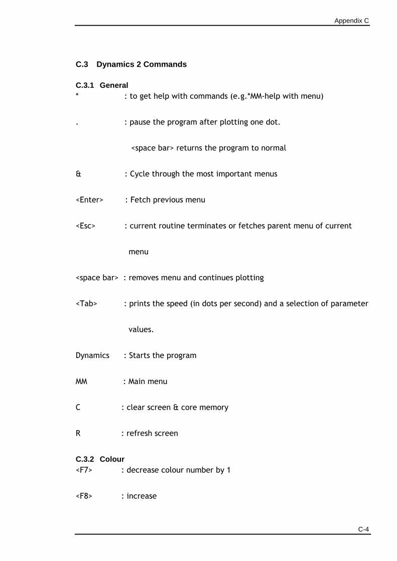
Appendix C
C-4
C.3 Dynamics 2 Commands
C.3.1 General * : to get help with commands (e.g.*MM-help with menu)
. : pause the program after plotting one dot.
<space bar> returns the program to normal
& : Cycle through the most important menus
<Enter> : Fetch previous menu
<Esc> : current routine terminates or fetches parent menu of current
menu
<space bar> : removes menu and continues plotting
<Tab> : prints the speed (in dots per second) and a selection of parameter
values.
Dynamics : Starts the program
MM : Main menu
C : clear screen & core memory
R : refresh screen
C.3.2 Colour <F7> : decrease colour number by 1
<F8> : increase
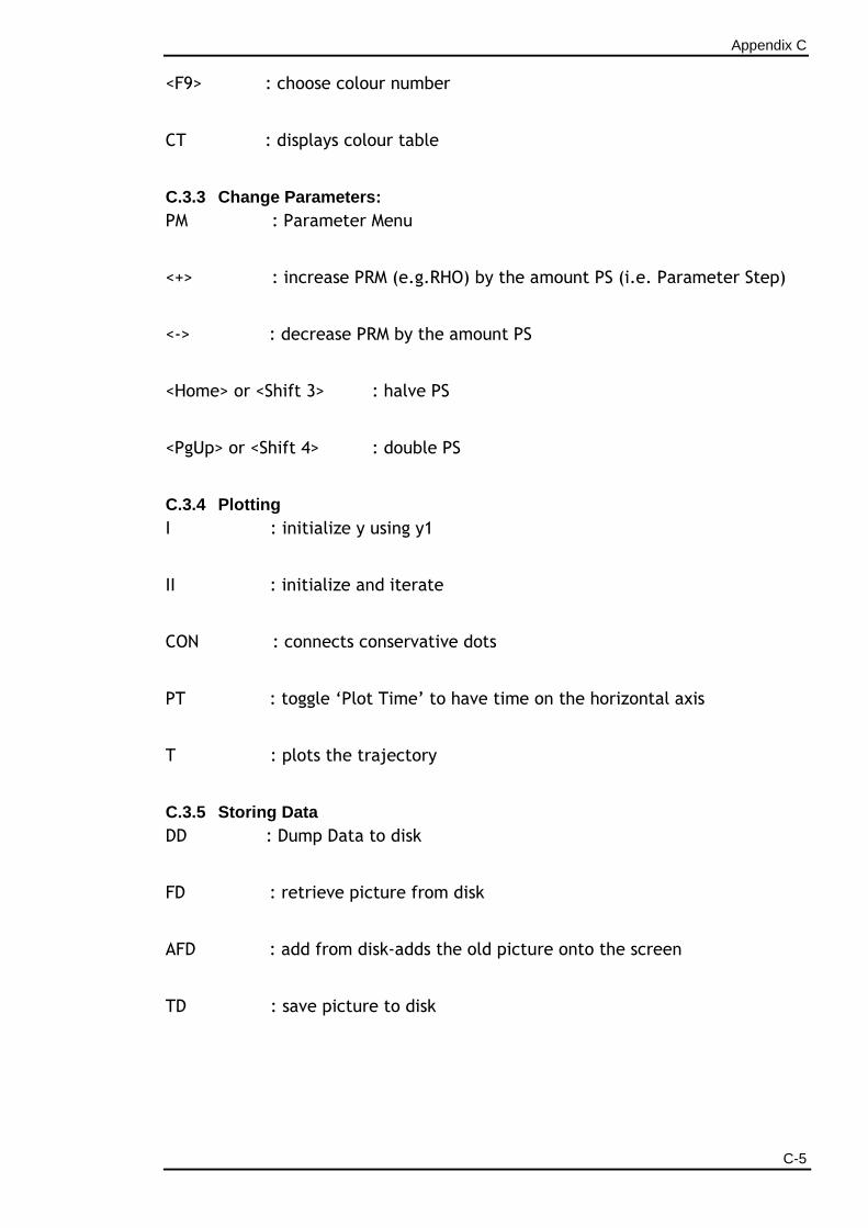
Appendix C
C-5
<F9> : choose colour number
CT : displays colour table
C.3.3 Change Parameters: PM : Parameter Menu
<+> : increase PRM (e.g.RHO) by the amount PS (i.e. Parameter Step)
<-> : decrease PRM by the amount PS
<Home> or <Shift 3> : halve PS
<PgUp> or <Shift 4> : double PS
C.3.4 Plotting I : initialize y using y1
II : initialize and iterate
CON : connects conservative dots
PT : toggle ‘Plot Time’ to have time on the horizontal axis
T : plots the trajectory
C.3.5 Storing Data DD : Dump Data to disk
FD : retrieve picture from disk
AFD : add from disk-adds the old picture onto the screen
TD : save picture to disk
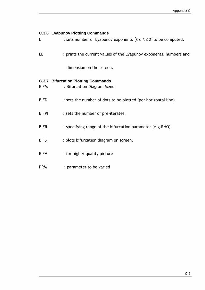
Appendix C
C-6
C.3.6 Lyapunov Plotting Commands
L : sets number of Lyapunov exponents ( )0 2L≤ ≤ to be computed.
LL : prints the current values of the Lyapunov exponents, numbers and
dimension on the screen.
C.3.7 Bifurcation Plotting Commands BIFM : Bifurcation Diagram Menu
BIFD : sets the number of dots to be plotted (per horizontal line).
BIFPI : sets the number of pre-iterates.
BIFR : specifying range of the bifurcation parameter (e.g.RHO).
BIFS : plots bifurcation diagram on screen.
BIFV : for higher quality picture
PRM : parameter to be varied
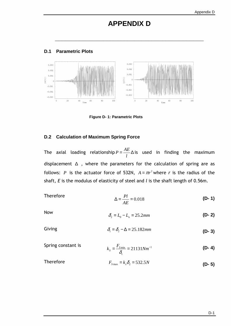
Appendix D
D-1
APPENDIX D
___________________________________________
D.1 Parametric Plots
0 20 40 60 80 100Time
-0.003
-0.002
-0.001
0
0.001
0.002
0.003
8x@t
D<
0 20 40 60 80 100
Time
-0.003
-0.002
-0.001
0
0.001
0.002
0.003
8y@t
D<
Figure D- 1: Parametric Plots
D.2 Calculation of Maximum Spring Force
The axial loading relationshipAE
Pl
= ∆ is used in finding the maximum
displacement ∆ , where the parameters for the calculation of spring are as
follows: P is the actuator force of 532N, 2A rπ= where r is the radius of the
shaft, E is the modulus of elasticity of steel and l is the shaft length of 0.56m.
Therefore 0.018
Pl
AE∆ = = (D- 1)
Now 2 0 25.2nL L mmδ = − =
(D- 2)
Giving 1 2 25.182mmδ δ= − ∆ = (D- 3)
Spring constant is 1min
1
21131SS
Fk Nm
δ−= = (D- 4)
Therefore max 2 532.5S sF k Nδ= = (D- 5)