Embed Size (px)
Citation preview
VIBRATION-BASED DAMAGE DETECTION ON A
MULTI-GIRDER BRIDGE SUPERSTRUCTURE
A Thesis
Submitted to the College of Graduate Studies and Research
in Partial Fulfillment of the Requirements
for the
Degree of Doctor of Philosophy
in the
Department of Civil and Geological Engineering
University of Saskatchewan
Saskatoon
By
Yufeng Wang
2011
© Copyright Yufeng Wang, September 2011. All rights reserved.

ii
PERMISSION TO USE
In presenting the thesis in partial fulfillment of the requirements for a postgraduate
degree from the University of Saskatchewan, I agree that the libraries of this University
may make it freely available for inspection. I further agree that permission for copying
of this thesis in any manner, in whole or in part, for scholarly purposes may be granted
by the professor who supervised my thesis work or, in his absence, by the Head of the
Department or the Dean of the College in which my thesis work was done. It is
understood that any copying or publication or use of this thesis or parts thereof for
financial gain shall not be allowed without my written permission. It is also understood
that due recognition shall be given to me and to the University of Saskatchewan in any
scholarly use which may be made of any material in my thesis.
Requests for permission to copy or to make other use of material in this thesis in whole
or part shall be addressed to:
Head of the Department of Civil and Geological Engineering
University of Saskatchewan
Saskatoon, Saskatchewan, S7N 5A9, Canada

iii
ABSTRACT
Vibration-based damage detection (VBDD) techniques have been proposed as a
potential form of structural health monitoring with which an entire structure can be
evaluated simultaneously using relatively few sensors. Since these methods rely on the
identification of small changes in dynamic properties (notably natural frequencies and
mode shapes) to infer the existence and the location of damage, reliable estimates of
these properties are essential for the successful implementation of VBDD schemes.
The research described in this thesis was primarily focused on an experimental
investigation of the application of VBDD on a multi-girder bridge superstructure, with
the objectives of identifying the most reliable test procedures, developing VBDD
techniques that could be used for identifying the presence of damage, and evaluating the
performance of VBDD techniques for such structures. The experimental investigation
was supplemented by theoretical analyses and numerical verifications. The structure
used for this investigation was a one-third scale model of a slab-on-girder composite
bridge superstructure featuring four steel girders supporting a steel-free concrete deck,
based on the North Perimeter Red River Bridge in Winnipeg, Manitoba.
The experimental tests were conducted in a well-controlled laboratory environment.
Forced dynamic excitation was supplied by means of a feedback-controlled hydraulic
shaker. Instrumentation used to measure the dynamic response included a closely-
spaced grid of accelerometers mounted on the surface of the deck along the girder lines,
as well as electrical-resistance foil strain gauges bonded to the girder webs. Damage
cases investigated included damage to the steel girders, to the diaphragm members, to
the lateral steel straps, and to the concrete deck.
A damage detection indicator was developed based on mode shapes that had been
normalized to enclose an area of unity. The resulting area under the plot of the
difference between two independently measured mode shapes was then used as the
damage indicator. To demonstrate the features and verify the capability of the newly
developed damage indicator in the absence of experimental uncertainties, a finite

iv
element model of the bridge superstructure was developed and used to generate
theoretical data for the modal properties.
A database of pairs of independently measured mode shapes, in which both mode
shapes in the pair were obtained with the structure in an identical condition, was used to
ascertain the variability of the area of mode shape change indicator when different test
procedures were followed. This allowed the definition of threshold values of the
damage indicator for each set of test procedures, corresponding to the 90th or 95th
percentile of the probability distribution of the damage indicator. When the damage
indicator exceeds this value, the presence of damage can be inferred with a high level of
confidence. A total of 28 different test protocols were investigated, which included two
different excitation methods (resonant harmonic and white noise random), four different
instrumentation schemes (accelerometers and strain gauges at various locations), and
five different vibration modes (the lowest five).
Five commonly available VBDD indicators were also selected to identify the location of
damage after its presence had been detected. The performance of the VBDD indicators
were examined and evaluated while two different normalization schemes were adopted.
The newly developed damage indicator, the area of mode shape change, was shown to
be capable of successfully identifying the presence of damage with a high confidence
level using both numerical and experimental data.
Of the 28 test protocols investigated, those that used forced harmonic excitation in
combination with the fundamental vibration mode consistently resulted in the lowest
threshold values for the area of mode shape change, and therefore resulted in the highest
sensitivity to the presence of damage.
The presence of most single damage scenarios could be identified with a relatively high
confidence level (at least 90%) when harmonic excitation was used, regardless of the
instrumentation scheme used to measure the mode shape (except for the scheme that
used data from strain gauges near the top flanges of the girders), since the area changes
in the fundamental mode shape due to damage exceeded the corresponding threshold

v
values. Among the instrumentation schemes investigated, both acceleration
measurements and measurements of flexural strains near the bottom flanges of the
girders were able to identify the presence of damage with a high level of confidence.
In general, all VBDD methods selected could localize the damage investigated with
varying degrees of accuracy when the fundamental mode was used, as long as the
presence of damage had previously been detected with a high confidence level.

vi
ACKNOWLEDGEMENTS
I wish to express sincerely my appreciation to my supervisors, Dr. Bruce Sparling and
Dr. Leon Wegner for their invaluable guidance, suggestions, encouragement, and
continuous assistance throughout the present study.
I also want to appreciate the advice from other members of my advisory committee: Dr.
Moh Boulfiza, Dr. Lisa Feldman, Dr. Allan Dolovich, and Dr. Amin Elshorbagy.
The help from the laboratory technicians in the Structures and Materials Laboratory, Mr.
Dale Pavier and Mr. Brennan Pokoyoway, is deeply appreciated. I also would like to
extend my gratitude to those staff in the university and friends who helped me during
this research.
Also, I would like to express my deepest and sincerest gratitude to my family, especially
my parents and my wife, Ying Chen, for their support and encouragement throughout
my life. This thesis is dedicated to our lovely little boy Luke to compensate a little bit
for the time spent on this thesis rather than him.

vii
TABLE OF CONTENTS
PERMISSION TO USE .................................................................................................... ii
ABSTRACT ............................................................................................................ iii
ACKNOWLEDGEMENTS ............................................................................................. vi
TABLE OF CONTENTS ................................................................................................ vii
LIST OF TABLES .......................................................................................................... xv
LIST OF FIGURES ..................................................................................................... xxvi
LIST OF SYMBOLS ....................................................................................................... lii
LIST OF ABBREVIATIONS .......................................................................................... lv
CHAPTER 1. INTRODUCTION ............................................................................... 1
1.1 Background ........................................................................................................ 1
1.2 Objectives ........................................................................................................... 3
1.3 Contributions to Original Knowledge ................................................................ 4
1.4 Scope and Methodology ..................................................................................... 5
1.5 Layout of the Thesis ........................................................................................... 7
CHAPTER 2. LITERATURE REVIEW .................................................................... 9
2.1 Overview ............................................................................................................ 9
2.2 Damage Detection ............................................................................................ 11
2.3 Dynamic Tests .................................................................................................. 13

viii
2.3.1 Overview ................................................................................................... 13
2.3.2 Dynamic excitation ................................................................................... 14
2.3.3 Sensors ...................................................................................................... 14
2.3.4 Noise and uncertainty in dynamic tests..................................................... 15
2.4 Signal Processing and Modal Analysis ............................................................ 17
2.4.1 Overview ................................................................................................... 17
2.4.2 Frequency domain modal analysis methods ............................................. 18
2.4.3 Time domain modal analysis methods ...................................................... 21
2.5 VBDD Methods ................................................................................................ 23
2.5.1 Overview ................................................................................................... 23
2.5.2 Change in mode shape method ................................................................. 25
2.5.3 Damage index method .............................................................................. 26
2.5.4 Change in flexibility method .................................................................... 27
2.5.5 Change in uniform flexibility curvature method....................................... 27
2.5.6 Change in mode shape curvature method ................................................. 28
2.6 Application of VBDD Methods to Bridges ...................................................... 29
2.7 VBDD Research Conducted at the University of Saskatchewan ..................... 33
2.8 Summary .......................................................................................................... 35
CHAPTER 3. EXPERIMENTAL PROGRAM ........................................................ 38
3.1 Description of Bridge Model ............................................................................ 38
ix
3.2 Measurement of Dynamic Properties ............................................................... 40
3.2.1 Overview ................................................................................................... 40
3.2.2 Instrumentation ......................................................................................... 43
3.2.2.1 Overview ................................................................................................ 43
3.2.2.2 Accelerometers ...................................................................................... 43
3.2.2.3 Strain gauges ......................................................................................... 47
3.2.3 Excitation force ......................................................................................... 50
3.2.4 Data acquisition ........................................................................................ 53
3.3 Data Processing ................................................................................................ 56
3.4 Description of Damage Cases .......................................................................... 60
3.5 Test Protocols Investigated .............................................................................. 65
CHAPTER 4. EXPERIMENTAL RESULTS .......................................................... 68
4.1 Overview .......................................................................................................... 68
4.2 Dynamic Properties of the Bridge Model......................................................... 69
4.2.1 Recorded vibration data and the corresponding modal identification ...... 69
4.2.2 Measured natural frequencies ................................................................... 76
4.2.3 Measured mode shapes ............................................................................. 83
4.2.4 Comparison of the measured mode shapes in different health states ....... 88
4.3 Influence of Test Parameters on Dynamic Properties ...................................... 88
4.3.1 Overview ................................................................................................... 88
x
4.3.2 Influence of sensor type and vertical location of strain gauges ................ 91
4.3.3 Influence of excitation type ...................................................................... 93
4.3.4 Influence of recording period and modal analysis method ....................... 94
4.3.5 Influence of sampling rate and data smoothing ...................................... 103
4.4 Influence of Normalization on Mode Shape Definition and Change in Mode
Shape Due to Damage .................................................................................... 106
4.4.1 Overview ................................................................................................. 106
4.4.2 Unit-norm normalization ........................................................................ 107
4.4.2.1 Definition of unit-norm normalization ................................................ 107
4.4.2.2 Application of the unit-norm normalization ........................................ 108
4.4.3 Unit-area normalization .......................................................................... 112
4.4.3.1 Definition of the unit-area normalization ........................................... 112
4.4.3.2 Application of unit-area normalization ............................................... 113
4.4.4 Different normalization schemes ............................................................ 118
CHAPTER 5. LEVEL 1 VBDD INDICATOR DEVELOPED: THE AREA OF
MODE SHAPE CHANGE .............................................................. 121
5.1 Overview ........................................................................................................ 121
5.2 Development of the Damage Indicator .......................................................... 122
5.2.1 Description of the damage indicator ....................................................... 122
5.2.2 Features of the new damage indicator .................................................... 123
xi
5.2.3 Differences between the area of mode shape change and “mode shape area
index” ............................................................................................................
................................................................................................................. 123
5.3 Verification of the Damage Indicator Using Numerical Data ........................ 124
5.3.1 Description of the finite element model .................................................. 124
5.3.2 Description of simulated health states and damage cases ....................... 127
5.3.3 Results and discussion ............................................................................ 129
5.3.3.1 Simulated model properties ................................................................. 129
5.3.3.2 Change in modal properties due to damage ....................................... 134
5.3.3.3 The area of mode shape change due to simulated damage cases ....... 137
CHAPTER 6. APPLICATION OF VBDD METHODS TO THE MULTI-GIRDER
BRIDGE SUPERSTRUCTURE ...................................................... 145
6.1 Overview ........................................................................................................ 145
6.2 Detection of the Presence of Damage Using the Area of Mode Shape Change
Damage Indicator ........................................................................................... 146
6.2.1 Overview ................................................................................................. 146
6.2.2 Distribution of the area of mode shape change when there is no change in
condition ................................................................................................. 146
6.2.3 Definition of the resolution of a specific test protocol............................ 158
6.2.4 Threshold values for different test procedures ........................................ 159
6.2.5 Detection of the presence of damage using the area of mode shape change
method based on the calculated probability values ................................. 163
xii
6.2.6 Detection of the presence of damage using the area of mode shape change
method based on the threshold values of test protocols .......................... 171
6.2.7 Influence of sensor scheme on the performance of the damage indicator ....
................................................................................................................. 175
6.2.8 Conclusions ............................................................................................. 181
6.3 Damage Localization Using Commonly Available VBDD Indicators .......... 183
6.3.1 Overview ................................................................................................. 183
6.3.2 Change in mode shape method ............................................................... 185
6.3.3 Damage index method ............................................................................ 187
6.3.4 Change in uniform flexibility curvature method..................................... 188
6.3.5 Change in flexibility method .................................................................. 191
6.3.6 Change in mode shape curvature method ............................................... 193
CHAPTER 7. SUMMARY AND CONCLUSIONS .............................................. 195
7.1 Summary ........................................................................................................ 195
7.2 Conclusions .................................................................................................... 197
7.3 Recommendations for Future Research ......................................................... 202
REFERENCES ......................................................................................................... 203
APPENDIX A. A PRELIMINARY FIELD TEST ON THE PROTOTYPE BRIDGE ..
......................................................................................................... 216
A.1 Overview ........................................................................................................ 216
A.2 Measurement of Dynamic Properties ............................................................. 217
xiii
APPENDIX B. PRELIMINARY NUMERICAL STUDIES .................................... 221
B.1 Introduction .................................................................................................... 221
B.2 Scaling Model with Gravitational Force Neglected ....................................... 221
B.3 Finite Element Verification for the Feasibility of the Scaling Model Method ....
........................................................................................................................ 223
B.4 Conclusions .................................................................................................... 224
APPENDIX C. FABRICATION OF EXPERIMENTAL MODEL ......................... 225
APPENDIX D. ADDITIONAL INFORMATION FOR INFLUENCE OF TEST
PARAMETERS ON DYNAMIC PROPERTIES ........................... 228
APPENDIX E. EVALUATION OF EXTRACTED DYNAMIC PROPERTIES .... 230
APPENDIX F. ADDITIONAL INFORMATION FOR THE FE MODEL ............. 268
APPENDIX G. ADDITIONAL INFORMATION FOR DISTRIBUTION OF THE
AREA OF MODE SHAPE CHANGE ............................................ 270
APPENDIX H. ADDITIONAL INFORMATION FOR DETECTION OF THE
PRESENCE OF DAMAGE ............................................................. 286
APPENDIX I. DETECTION OF DAMAGE CASE 1 USING COMMONLY
AVAILABLE VBDD INDICATORS BASED ON THE FIRST
MODE SHAPE ................................................................................ 388
APPENDIX J. DETECTION OF DAMAGE CASE 1 USING HIGHER
VIBRATION MODES WHEN ACCELEROMETER DATA AND
WHITE NOISE RANDOM EXCITATION WERE USED ............ 400
APPENDIX K. DAMAGE DETECTION USING CHANGE IN THE FIRST MODE
SHAPE FOR DAMAGE CASES 2 TO 16 WHEN
xiv
ACCELEROMETER DATA AND HARMONIC EXCITATION
WERE USED .................................................................................. 412
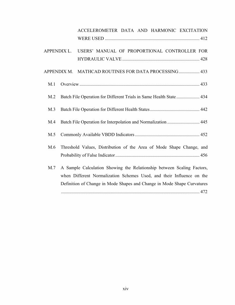
APPENDIX L. USERS’ MANUAL OF PROPORTIONAL CONTROLLER FOR
HYDRAULIC VALVE ................................................................... 428
APPENDIX M. MATHCAD ROUTINES FOR DATA PROCESSING .................. 433
M.1 Overview ........................................................................................................ 433
M.2 Batch File Operation for Different Trials in Same Health State .................... 434
M.3 Batch File Operation for Different Health States ........................................... 442
M.4 Batch File Operation for Interpolation and Normalization ............................ 445
M.5 Commonly Available VBDD Indicators ........................................................ 452
M.6 Threshold Values, Distribution of the Area of Mode Shape Change, and
Probability of False Indicator ......................................................................... 456
M.7 A Sample Calculation Showing the Relationship between Scaling Factors,
when Different Normalization Schemes Used, and their Influence on the
Definition of Change in Mode Shapes and Change in Mode Shape Curvatures
........................................................................................................................ 472

xv
LIST OF TABLES
Table 3.1. The summary of the test program. ................................................................... 42
Table 3.2. The summary of accelerometer calibration factors from 20 trials. .................. 45
Table 3.3. The summary of setups of accelerometers with a common reference channel.47
Table 3.4. The health states investigated on the bridge model. ........................................ 63
Table 3.5. The summary of damage cases considered for the bridge model. ................... 66
Table 3.6. The summary of test protocols investigated. ................................................... 67
Table 4.1. Measured natural frequencies using accelerometers for Health State 1. ......... 79
Table 4.2. Measured natural frequencies using strain gauges for Health State 1. ............ 80
Table 4.3. Comparison of measured frequencies in different health states based on
accelerometer and strain gauge data. ................................................................................ 81
Table 4.4. Influence of sensor group on mode shape reliability based on averaged MAC
values from five repeated trials with white noise random excitation. .............................. 92
Table 4.5. Influence of excitation type on mode shape reliability based on averaged
MAC values using accelerometer data from five replicate trials. ..................................... 93
Table 4.6. Influence of recording period on the repeatability of the fundamental mode
shape based on averaged MAC values from five repeated trials with harmonic excitation
and sampling rate of 200 Hz. ............................................................................................ 96
Table 4.7. Influence of recording period on the repeatability of the fundamental mode
shape based on averaged MAC values from five repeated trials with white noise random
excitation and sampling rate of 200 Hz. ........................................................................... 99
xvi
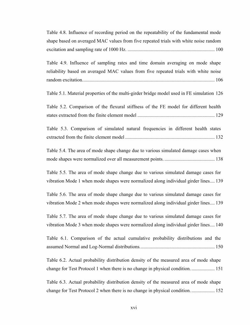
Table 4.8. Influence of recording period on the repeatability of the fundamental mode
shape based on averaged MAC values from five repeated trials with white noise random
excitation and sampling rate of 1000 Hz. ....................................................................... 100
Table 4.9. Influence of sampling rates and time domain averaging on mode shape
reliability based on averaged MAC values from five repeated trials with white noise
random excitation. ........................................................................................................... 106
Table 5.1. Material properties of the multi-girder bridge model used in FE simulation 126
Table 5.2. Comparison of the flexural stiffness of the FE model for different health
states extracted from the finite element model ............................................................... 129
Table 5.3. Comparison of simulated natural frequencies in different health states
extracted from the finite element model ......................................................................... 132
Table 5.4. The area of mode shape change due to various simulated damage cases when
mode shapes were normalized over all measurement points. ......................................... 138
Table 5.5. The area of mode shape change due to various simulated damage cases for
vibration Mode 1 when mode shapes were normalized along individual girder lines. ... 139
Table 5.6. The area of mode shape change due to various simulated damage cases for
vibration Mode 2 when mode shapes were normalized along individual girder lines. ... 139
Table 5.7. The area of mode shape change due to various simulated damage cases for
vibration Mode 3 when mode shapes were normalized along individual girder lines. ... 140
Table 6.1. Comparison of the actual cumulative probability distributions and the
assumed Normal and Log-Normal distributions. ............................................................ 150
Table 6.2. Actual probability distribution density of the measured area of mode shape
change for Test Protocol 1 when there is no change in physical condition. ................... 151
Table 6.3. Actual probability distribution density of the measured area of mode shape
change for Test Protocol 2 when there is no change in physical condition. ................... 152
xvii
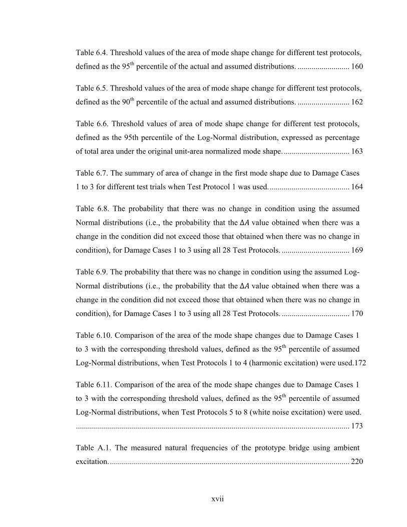
Table 6.4. Threshold values of the area of mode shape change for different test protocols,
defined as the 95th percentile of the actual and assumed distributions. .......................... 160
Table 6.5. Threshold values of the area of mode shape change for different test protocols,
defined as the 90th percentile of the actual and assumed distributions. .......................... 162
Table 6.6. Threshold values of area of mode shape change for different test protocols,
defined as the 95th percentile of the Log-Normal distribution, expressed as percentage
of total area under the original unit-area normalized mode shape. ................................. 163
Table 6.7. The summary of area of change in the first mode shape due to Damage Cases
1 to 3 for different test trials when Test Protocol 1 was used. ........................................ 164
Table 6.8. The probability that there was no change in condition using the assumed
Normal distributions (i.e., the probability that the Δ value obtained when there was a
change in the condition did not exceed those that obtained when there was no change in
condition), for Damage Cases 1 to 3 using all 28 Test Protocols. .................................. 169
Table 6.9. The probability that there was no change in condition using the assumed Log-
Normal distributions (i.e., the probability that the Δ value obtained when there was a
change in the condition did not exceed those that obtained when there was no change in
condition), for Damage Cases 1 to 3 using all 28 Test Protocols. .................................. 170
Table 6.10. Comparison of the area of the mode shape changes due to Damage Cases 1
to 3 with the corresponding threshold values, defined as the 95th percentile of assumed
Log-Normal distributions, when Test Protocols 1 to 4 (harmonic excitation) were used.172
Table 6.11. Comparison of the area of the mode shape changes due to Damage Cases 1
to 3 with the corresponding threshold values, defined as the 95th percentile of assumed
Log-Normal distributions, when Test Protocols 5 to 8 (white noise excitation) were used.
......................................................................................................................................... 173
Table A.1. The measured natural frequencies of the prototype bridge using ambient
excitation. ........................................................................................................................ 220

xviii
Table B.1. Similitude requirements for the scale bridge model. .................................... 222
Table B.2. The natural frequencies (Hz) of the undamaged 4-girder steel free bridge
deck. ................................................................................................................................ 224
Table B.3. The natural frequencies (Hz) for a single-damage case on the 4-girder steel
free bridge deck. .............................................................................................................. 224
Table C.1. The measured compressive strength of concrete samples used for the bridge
deck. ................................................................................................................................ 225
Table D.1. Influence of excitation type on mode shape reliability based on averaged
MAC values using bottom strain gauge data from five replicate trials. ......................... 228
Table D.2. Influence of excitation type on mode shape reliability based on averaged
MAC values using middle strain gauge data from five replicate trials. .......................... 229
Table D.3. Influence of excitation type on mode shape reliability based on averaged
MAC values using top strain gauge data from five replicate trials. ................................ 229
Table E.1. Measured natural frequencies using accelerometers for Health State 2. ....... 231
Table E.2. Measured natural frequencies using accelerometers for Health State 3. ....... 232
Table E.3. Measured natural frequencies using accelerometers for Health State 4. ....... 233
Table E.4. Measured natural frequencies using accelerometers for Health State 5. ....... 234
Table E.5. Measured natural frequencies using accelerometers for Health State 6. ....... 235
Table E.6. Measured natural frequencies using accelerometers for Health State 7. ....... 236
Table E.7. Measured natural frequencies using accelerometers for Health State 8. ....... 237
Table E.8. Measured natural frequencies using accelerometers for Health State 9. ....... 238
Table E.9. Measured natural frequencies using accelerometers for Health State 10. ..... 239

xix
Table E.10. Measured natural frequencies using accelerometers for Health State 11. ... 240
Table E.11. Measured natural frequencies using accelerometers for Health State 12. ... 241
Table E.12. Measured natural frequencies using accelerometers for Health State 13. ... 242
Table E.13. Measured natural frequencies using accelerometers for Health State 14. ... 243
Table E.14. Measured natural frequencies using accelerometers for Health State 15. ... 244
Table E.15. Measured natural frequencies using accelerometers for Health State 16. ... 245
Table E.16. Measured natural frequencies using accelerometers for Health State 17. ... 246
Table E.17. Measured natural frequencies using strain gauges for Health State 2. ........ 247
Table E.18. Measured natural frequencies using strain gauges for Health State 3. ........ 247
Table E.19. Measured natural frequencies using strain gauges for Health State 4. ........ 248
Table E.20. Measured natural frequencies using strain gauges for Health State 5. ........ 248
Table E.21. Measured natural frequencies using strain gauges for Health State 6. ........ 249
Table E.22. Measured natural frequencies using strain gauges for Health State 7. ........ 249
Table E.23. Measured natural frequencies using strain gauges for Health State 8. ........ 250
Table E.24. Measured natural frequencies using strain gauges for Health State 9. ........ 250
Table E.25. Measured natural frequencies using strain gauges for Health State 10. ...... 251
Table E.26. Measured natural frequencies using strain gauges for Health State 11. ...... 251
Table E.27. Measured natural frequencies using strain gauges for Health State 12. ...... 252
Table E.28. Measured natural frequencies using strain gauges for Health State 13. ...... 252
Table E.29. Measured natural frequencies using strain gauges for Health State 14. ...... 253
xx
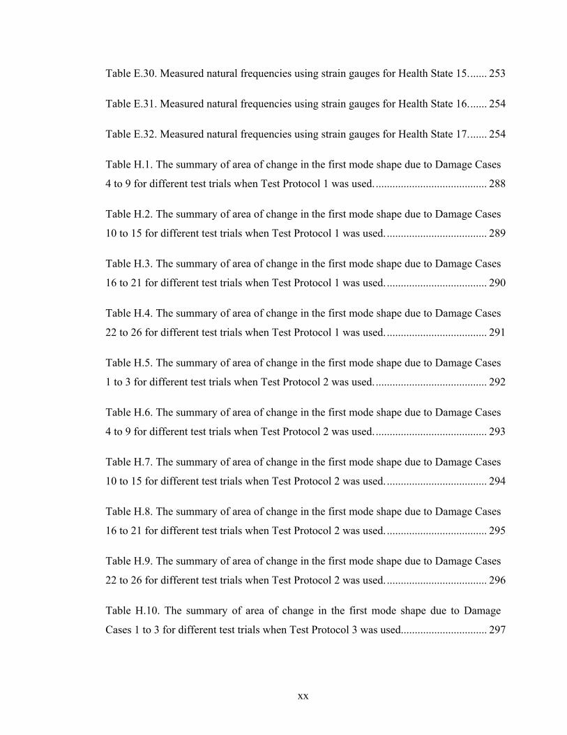
Table E.30. Measured natural frequencies using strain gauges for Health State 15. ...... 253
Table E.31. Measured natural frequencies using strain gauges for Health State 16. ...... 254
Table E.32. Measured natural frequencies using strain gauges for Health State 17. ...... 254
Table H.1. The summary of area of change in the first mode shape due to Damage Cases
4 to 9 for different test trials when Test Protocol 1 was used. ........................................ 288
Table H.2. The summary of area of change in the first mode shape due to Damage Cases
10 to 15 for different test trials when Test Protocol 1 was used. .................................... 289
Table H.3. The summary of area of change in the first mode shape due to Damage Cases
16 to 21 for different test trials when Test Protocol 1 was used. .................................... 290
Table H.4. The summary of area of change in the first mode shape due to Damage Cases
22 to 26 for different test trials when Test Protocol 1 was used. .................................... 291
Table H.5. The summary of area of change in the first mode shape due to Damage Cases
1 to 3 for different test trials when Test Protocol 2 was used. ........................................ 292
Table H.6. The summary of area of change in the first mode shape due to Damage Cases
4 to 9 for different test trials when Test Protocol 2 was used. ........................................ 293
Table H.7. The summary of area of change in the first mode shape due to Damage Cases
10 to 15 for different test trials when Test Protocol 2 was used. .................................... 294
Table H.8. The summary of area of change in the first mode shape due to Damage Cases
16 to 21 for different test trials when Test Protocol 2 was used. .................................... 295
Table H.9. The summary of area of change in the first mode shape due to Damage Cases
22 to 26 for different test trials when Test Protocol 2 was used. .................................... 296
Table H.10. The summary of area of change in the first mode shape due to Damage
Cases 1 to 3 for different test trials when Test Protocol 3 was used............................... 297
xxi
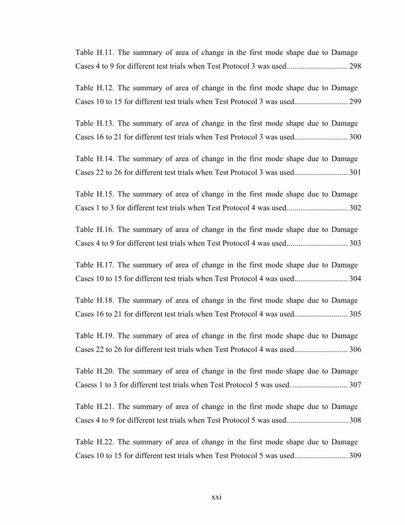
Table H.11. The summary of area of change in the first mode shape due to Damage
Cases 4 to 9 for different test trials when Test Protocol 3 was used............................... 298
Table H.12. The summary of area of change in the first mode shape due to Damage
Cases 10 to 15 for different test trials when Test Protocol 3 was used........................... 299
Table H.13. The summary of area of change in the first mode shape due to Damage
Cases 16 to 21 for different test trials when Test Protocol 3 was used........................... 300
Table H.14. The summary of area of change in the first mode shape due to Damage
Cases 22 to 26 for different test trials when Test Protocol 3 was used........................... 301
Table H.15. The summary of area of change in the first mode shape due to Damage
Cases 1 to 3 for different test trials when Test Protocol 4 was used............................... 302
Table H.16. The summary of area of change in the first mode shape due to Damage
Cases 4 to 9 for different test trials when Test Protocol 4 was used............................... 303
Table H.17. The summary of area of change in the first mode shape due to Damage
Cases 10 to 15 for different test trials when Test Protocol 4 was used........................... 304
Table H.18. The summary of area of change in the first mode shape due to Damage
Cases 16 to 21 for different test trials when Test Protocol 4 was used........................... 305
Table H.19. The summary of area of change in the first mode shape due to Damage
Cases 22 to 26 for different test trials when Test Protocol 4 was used........................... 306
Table H.20. The summary of area of change in the first mode shape due to Damage
Casess 1 to 3 for different test trials when Test Protocol 5 was used. ............................ 307
Table H.21. The summary of area of change in the first mode shape due to Damage
Cases 4 to 9 for different test trials when Test Protocol 5 was used............................... 308
Table H.22. The summary of area of change in the first mode shape due to Damage
Cases 10 to 15 for different test trials when Test Protocol 5 was used........................... 309

xxii
Table H.23. The summary of area of change in the first mode shape due to Damage
Cases 16 to 21 for different test trials when Test Protocol 5 was used........................... 310
Table H.24. The summary of area of change in the first mode shape due to Damage
Cases 22 to 26 for different test trials when Test Protocol 5 was used........................... 311
Table H.25. The summary of area of change in the first mode shape due to Damage
Cases 1 to 3 for different test trials when Test Protocol 6 was used............................... 312
Table H.26. The summary of area of change in the first mode shape due to Damage
Cases 4 to 9 for different test trials when Test Protocol 6 was used............................... 313
Table H.27. The summary of area of change in the first mode shape due to Damage
Cases 10 to 15 for different test trials when Test Protocol 6 was used........................... 314
Table H.28. The summary of area of change in the first mode shape due to Damage
Cases 16 to 21 for different test trials when Test Protocol 6 was used........................... 315
Table H.29. The summary of area of change in the first mode shape due to Damage
Cases 22 to 26 for different test trials when Test Protocol 6 was used........................... 316
Table H.30. The summary of area of change in the first mode shape due to Damage
Cases 1 to 3 for different test trials when Test Protocol 7 was used............................... 317
Table H.31. The summary of area of change in the first mode shape due to Damage
Cases 4 to 9 for different test trials when Test Protocol 7 was used............................... 318
Table H.32. The summary of area of change in the first mode shape due to Damage
Cases 10 to 15 for different test trials when Test Protocol 7 was used........................... 319
Table H.33. The summary of area of change in the first mode shape due to Damage
Cases 16 to 21 for different test trials when Test Protocol 7 was used........................... 320
Table H.34. The summary of area of change in the first mode shape due to Damage
Cases 22 to 26 for different test trials when Test Protocol 7 was used........................... 321
xxiii
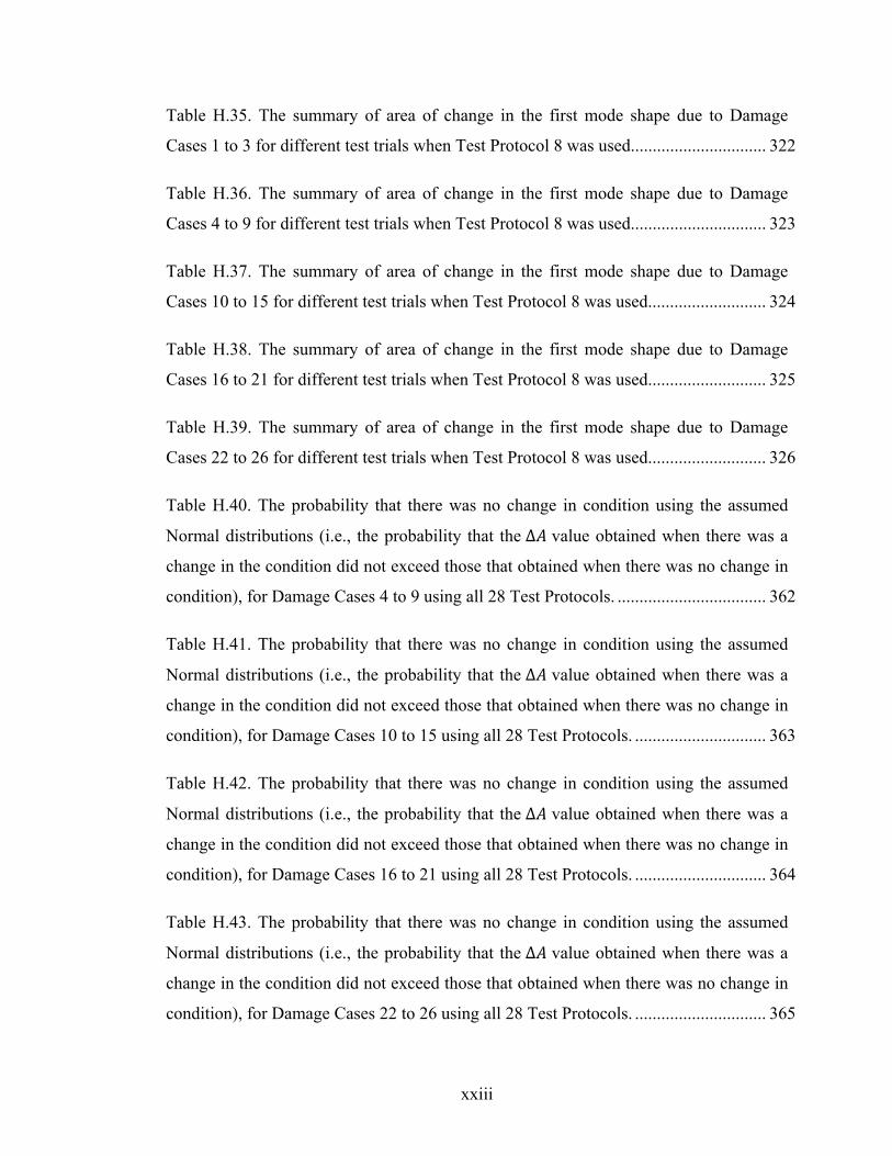
Table H.35. The summary of area of change in the first mode shape due to Damage
Cases 1 to 3 for different test trials when Test Protocol 8 was used............................... 322
Table H.36. The summary of area of change in the first mode shape due to Damage
Cases 4 to 9 for different test trials when Test Protocol 8 was used............................... 323
Table H.37. The summary of area of change in the first mode shape due to Damage
Cases 10 to 15 for different test trials when Test Protocol 8 was used........................... 324
Table H.38. The summary of area of change in the first mode shape due to Damage
Cases 16 to 21 for different test trials when Test Protocol 8 was used........................... 325
Table H.39. The summary of area of change in the first mode shape due to Damage
Cases 22 to 26 for different test trials when Test Protocol 8 was used........................... 326
Table H.40. The probability that there was no change in condition using the assumed
Normal distributions (i.e., the probability that the Δ value obtained when there was a
change in the condition did not exceed those that obtained when there was no change in
condition), for Damage Cases 4 to 9 using all 28 Test Protocols. .................................. 362
Table H.41. The probability that there was no change in condition using the assumed
Normal distributions (i.e., the probability that the Δ value obtained when there was a
change in the condition did not exceed those that obtained when there was no change in
condition), for Damage Cases 10 to 15 using all 28 Test Protocols. .............................. 363
Table H.42. The probability that there was no change in condition using the assumed
Normal distributions (i.e., the probability that the Δ value obtained when there was a
change in the condition did not exceed those that obtained when there was no change in
condition), for Damage Cases 16 to 21 using all 28 Test Protocols. .............................. 364
Table H.43. The probability that there was no change in condition using the assumed
Normal distributions (i.e., the probability that the Δ value obtained when there was a
change in the condition did not exceed those that obtained when there was no change in
condition), for Damage Cases 22 to 26 using all 28 Test Protocols. .............................. 365
xxiv
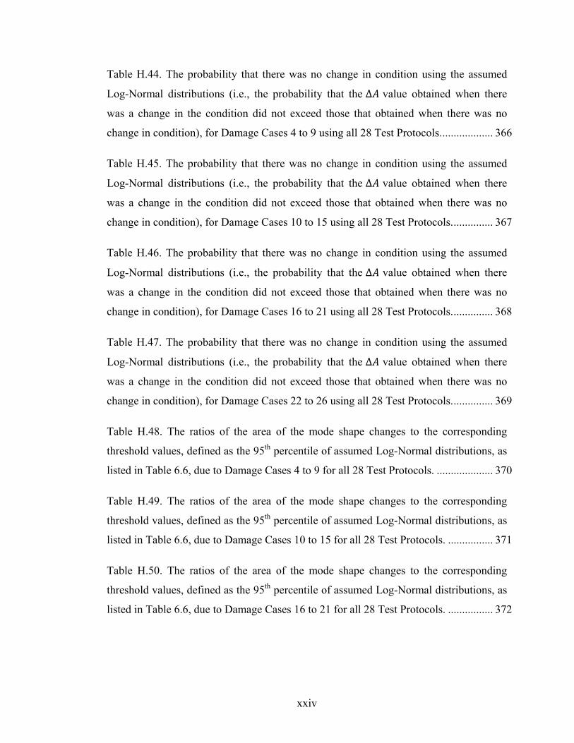
Table H.44. The probability that there was no change in condition using the assumed
Log-Normal distributions (i.e., the probability that the Δ value obtained when there
was a change in the condition did not exceed those that obtained when there was no
change in condition), for Damage Cases 4 to 9 using all 28 Test Protocols. .................. 366
Table H.45. The probability that there was no change in condition using the assumed
Log-Normal distributions (i.e., the probability that the Δ value obtained when there
was a change in the condition did not exceed those that obtained when there was no
change in condition), for Damage Cases 10 to 15 using all 28 Test Protocols. .............. 367
Table H.46. The probability that there was no change in condition using the assumed
Log-Normal distributions (i.e., the probability that the Δ value obtained when there
was a change in the condition did not exceed those that obtained when there was no
change in condition), for Damage Cases 16 to 21 using all 28 Test Protocols. .............. 368
Table H.47. The probability that there was no change in condition using the assumed
Log-Normal distributions (i.e., the probability that the Δ value obtained when there
was a change in the condition did not exceed those that obtained when there was no
change in condition), for Damage Cases 22 to 26 using all 28 Test Protocols. .............. 369
Table H.48. The ratios of the area of the mode shape changes to the corresponding
threshold values, defined as the 95th percentile of assumed Log-Normal distributions, as
listed in Table 6.6, due to Damage Cases 4 to 9 for all 28 Test Protocols. .................... 370
Table H.49. The ratios of the area of the mode shape changes to the corresponding
threshold values, defined as the 95th percentile of assumed Log-Normal distributions, as
listed in Table 6.6, due to Damage Cases 10 to 15 for all 28 Test Protocols. ................ 371
Table H.50. The ratios of the area of the mode shape changes to the corresponding
threshold values, defined as the 95th percentile of assumed Log-Normal distributions, as
listed in Table 6.6, due to Damage Cases 16 to 21 for all 28 Test Protocols. ................ 372

xxv
Table H.51. The ratios of the area of the mode shape changes to the corresponding
threshold values, defined as the 95th percentile of assumed Log-Normal distributions, as
listed in Table 6.6, due to Damage Cases 22 to 26 for all 28 Test Protocols. ................ 373

xxvi
LIST OF FIGURES
Figure 2.1. Variation of the dynamic amplification factor with the frequency ratio
( / 0). ............................................................................................................................. 20
Figure 3.1. Slab on girder bridge superstructure built at 1/3rd scale (with inset showing
the girder splice). .............................................................................................................. 38
Figure 3.2. Plan and cross-section view of the composite bridge deck showing the
structural components and general layout (dimensions in mm). ...................................... 39
Figure 3.3. Plan view of the structural steel superstructure of the model showing splice,
steel strap, and diaphragm locations (dimension in mm). ................................................ 40
Figure 3.4. EpiSensor FBA ES-U accelerometer. ............................................................. 44
Figure 3.5. Calibration of the EpiSensor FBA ES-U accelerometers for mode shape
measurement. .................................................................................................................... 44
Figure 3.6. The locations of acceleration measurement points (dimensions in mm)........ 46
Figure 3.7. Plan view of bridge deck, showing the locations of strain gauge clusters
(dimensions in mm). ......................................................................................................... 48
Figure 3.8. KYOWA KFG-6-120-C1-11L3M3R electronic strain gauges bonded on the
girder web of the bridge deck. .......................................................................................... 49
Figure 3.9. Setup of the strain gauge sets on the girder web (19 typical, dimensions in
mm). .................................................................................................................................. 49
Figure 3.10. The hydraulic frame-mounted shaker used for preliminary tests. ................ 51
Figure 3.11. The hydraulic shaker used to excite both resonant harmonic and white noise
random vibration in the experiments. ............................................................................... 52
Figure 3.12. Data acquisition system. ............................................................................... 55
xxvii
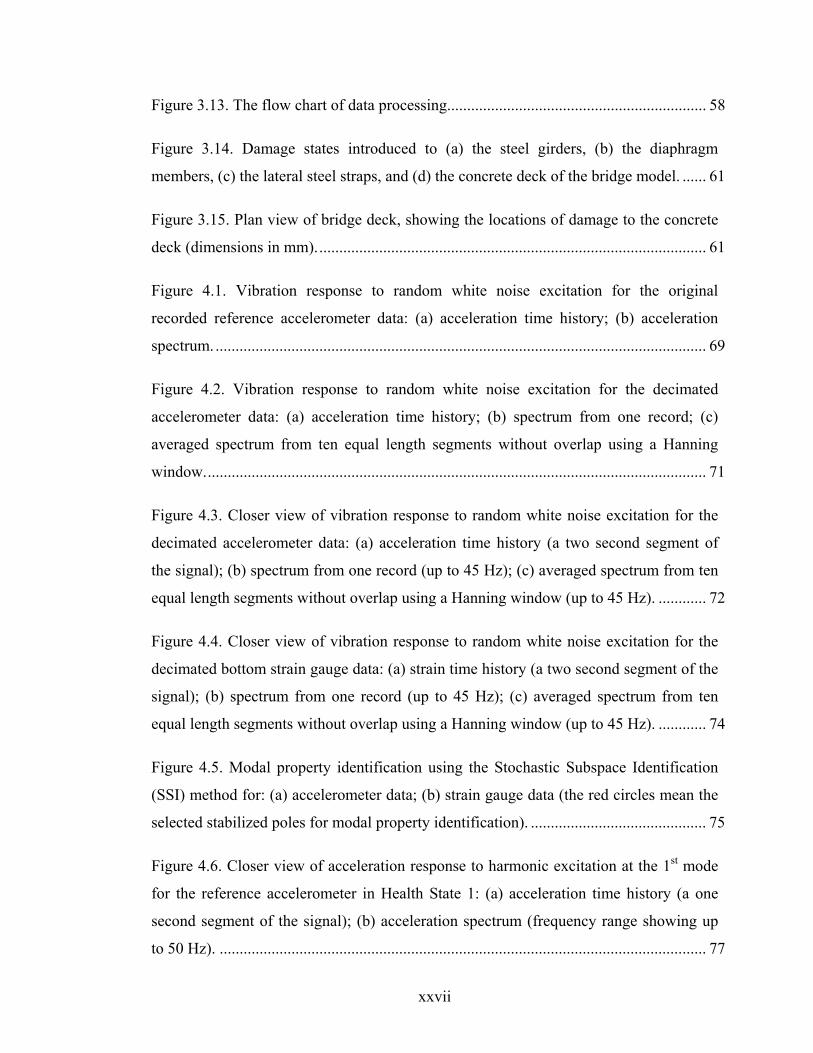
Figure 3.13. The flow chart of data processing................................................................. 58
Figure 3.14. Damage states introduced to (a) the steel girders, (b) the diaphragm
members, (c) the lateral steel straps, and (d) the concrete deck of the bridge model. ...... 61
Figure 3.15. Plan view of bridge deck, showing the locations of damage to the concrete
deck (dimensions in mm). ................................................................................................. 61
Figure 4.1. Vibration response to random white noise excitation for the original
recorded reference accelerometer data: (a) acceleration time history; (b) acceleration
spectrum. ........................................................................................................................... 69
Figure 4.2. Vibration response to random white noise excitation for the decimated
accelerometer data: (a) acceleration time history; (b) spectrum from one record; (c)
averaged spectrum from ten equal length segments without overlap using a Hanning
window. ............................................................................................................................. 71
Figure 4.3. Closer view of vibration response to random white noise excitation for the
decimated accelerometer data: (a) acceleration time history (a two second segment of
the signal); (b) spectrum from one record (up to 45 Hz); (c) averaged spectrum from ten
equal length segments without overlap using a Hanning window (up to 45 Hz). ............ 72
Figure 4.4. Closer view of vibration response to random white noise excitation for the
decimated bottom strain gauge data: (a) strain time history (a two second segment of the
signal); (b) spectrum from one record (up to 45 Hz); (c) averaged spectrum from ten
equal length segments without overlap using a Hanning window (up to 45 Hz). ............ 74
Figure 4.5. Modal property identification using the Stochastic Subspace Identification
(SSI) method for: (a) accelerometer data; (b) strain gauge data (the red circles mean the
selected stabilized poles for modal property identification). ............................................ 75
Figure 4.6. Closer view of acceleration response to harmonic excitation at the 1st mode
for the reference accelerometer in Health State 1: (a) acceleration time history (a one
second segment of the signal); (b) acceleration spectrum (frequency range showing up
to 50 Hz). .......................................................................................................................... 77

xxviii
Figure 4.7. Closer view of vibration response to harmonic excitation at the 1st mode for
a bottom strain gauge near mid-span for Health State 1: (a) strain time history (a one
second segment of the signal); (b) strain spectrum (frequency range showing up to 50
Hz). .................................................................................................................................... 78
Figure 4.8. The lowest five vibration mode shapes for Health State 1 based on
accelerometer data: (a) Mode 1, (b) Mode 2, (c) Mode 3, (d) Mode 4, and (e) Mode 5. . 84
Figure 4.9. The lowest five vibration mode shapes for Health State 1 based on bottom
strain gauge data: (a) Mode 1, (b) Mode 2, (c) Mode 3, (d) Mode 4, and (e) Mode 5. ... 85
Figure 4.10. The lowest five vibration mode shapes for Health State 1 based on
accelerometer data with white noise random excitation: (a) Mode 1, (b) Mode 2, (c)
Mode 3, (d) Mode 4, and (e) Mode 5. ............................................................................... 87
Figure 4.11. Comparison of the first mode shape for different health states using
accelerometer data with harmonic excitation.................................................................... 89
Figure 4.12. Comparison of the second mode shape for different health states using
accelerometer data with harmonic excitation.................................................................... 90
Figure 4.13. Influence of recording period on mode shape definition for resonant
harmonic excitation when both (a) SSI and (b) PP methods were used to extract modal
properties. .......................................................................................................................... 95
Figure 4.14. Influence of recording period on mode shape definition for white noise
random excitation with sampling rate of 200 Hz when the SSI method was used to
extract modal properties. ................................................................................................... 97
Figure 4.15. Influence of recording period on mode shape definition for white noise
random excitation with sampling rate of 200 Hz when the PP method was used to
extract modal properties. ................................................................................................... 98
xxix
Figure 4.16. Influence of recording period on mode shape definition for white noise
random excitation with sampling rate of 1000 Hz when SSI method was used to extract
modal properties. ............................................................................................................. 101
Figure 4.17. Influence of recording period on mode shape definition for white noise
random excitation with sampling rate of 1000 Hz when PP method was used to extract
modal properties. ............................................................................................................. 102
Figure 4.18. Influence of sampling rate on mode shape definition of: (a) Mode 1; (b)
Mode 2 for white noise random excitation with recording period of 80 seconds, when
the SSI method was used to extract modal properties. ................................................... 104
Figure 4.19. Influence of sampling rate on mode shape definition of: (a) Mode 3; (b)
Mode 4; (c) Mode 5 for white noise random excitation with recording period of 80
seconds, when the SSI method was used to extract modal properties. ........................... 105
Figure 4.20. Influence of unit-norm normalization on: (a) Mode 1 in Health State 1, (b)
Mode 1 in Health State 2, and (c) Change in mode shape for Damage Case 1, when
different number of measurement points is used. ........................................................... 109
Figure 4.21. Influence of unit-norm normalization on: (a) Mode 1 in Health State 1, (b)
Mode 1 in Health State 2, and (c) Change in mode shape in Damage Case 1, when
different measurement locations are used. ...................................................................... 110
Figure 4.22. Definition of unit-area normalization method: (a) the original unit-norm
normalized mode shape; (b) the individual mode shapes in (a) are strung end to end to
create a single mode shape vector, with the resulting length adjusted to be equal to one;
and (c) the mode shape in (b) is scaled to make the enclosed area equal to unity. ......... 114
Figure 4.23. Influence of unit-area normalization on: (a) Mode 1 in Health State 1, (b)
Mode 1 in Health State 2, and (c) Change in mode shape for Damage Case 1, when
different numbers of measurement points is used. .......................................................... 116

xxx
Figure 4.24. Influence of unit-area normalization on: (a) Mode 1 in Health State 1, (b)
Mode 1 in Health State 2, and (c) Change in mode shape for Damage Case 1, when
different measurement locations are used. ...................................................................... 117
Figure 4.25. Influence of the different normalization schemes on the definition of mode
shapes and changes in mode shapes due to Damage Case 1 for the fundamental mode
shape using the unit-area normalization: (a) over all measurement points; and (b) along
individual girder lines; (c) the change in fundamental mode shape due to Damage Case
1 using the unit-area normalization over all measurement points; and (d) along
individual girder lines. .................................................................................................... 120
Figure 5.1. The finite element model of the experimental bridge model showing: (a) the
whole finished model; and (b) the structural steel superstructure including the splice,
steel straps, diaphragms, and shear studs. ....................................................................... 125
Figure 5.2. The simulated damage states incrementally introduced to steel Girder 4 at
the splice connection: (a) Health State 1 (the intact condition), (b) Health State 2 (or
Damage Case 1), (c) Health State 11 (or Damage Case 10), and (d) Health State 12 (or
Damage Case 11). ........................................................................................................... 128
Figure 5.3. The simulated damage states incrementally introduced to the concrete deck
at a location near mid-span of Girders 3 and 4 for Health States 3 to 10, respectively,
with: (a) one, (b) two, (c) three, (d) four, (e) five, (f) six, (g) seven, and (f) eight
elements (100 X 100 X 25 mm) removed from the surface of the simulated concrete
deck. ................................................................................................................................ 130
Figure 5.4. The finite element model of the experimental bridge model: (a) the whole
meshed model; and (b) the physical model (before meshing), showing dimensions in
mm; with an inset showing the order of the removed elements in Health States 3 to 10.131
Figure 5.5. The lowest five vibration mode shapes for Health State 1 (the undamaged
condition) extracted from the finite element model: (a) Mode 1, (b) Mode 2, (c) Mode 3,
(d) Mode 4, and (e) Mode 5. ........................................................................................... 133

xxxi
Figure 5.6. The normalized mode shape of Mode 1 using the normalization scheme over
all measurement points for: (a) simulated Health State 1 and (b) simulated Health State
2. ...................................................................................................................................... 134
Figure 5.7. The normalized mode shape of Mode 1 using the normalization scheme
along individual girder lines for: (a) simulated Health State 1 and (b) simulated Health
State 2. ............................................................................................................................. 135
Figure 5.8. Change in mode shape due to the simulated Damage Case 1 using the
normalization schemes: (a) over all measurement points and (b) along the individual
girder lines. ..................................................................................................................... 137
Figure 5.9. Relationship between the area of mode shape change and the relative
flexural stiffness change due to damage for: (a) Mode 1, (b) Mode 2, and (c) Mode 3
when mode shapes were normalized over all measurement points. ............................... 143
Figure 5.10. Relationship between the area of mode shape change and the relative
flexural stiffness change due to damage for: (a) Mode 1, (b) Mode 2, and (c) Mode 3
when mode shapes were normalized along individual girder lines. ............................... 144
Figure 6.1. Comparison of the actual cumulative probability distributions and the
assumed Normal and Log-Normal distributions of Δ , for Test Protocols: (a) 1, (b) 2,
(c) 3, and (d) 4. ................................................................................................................ 148
Figure 6.2. Comparison of the actual cumulative probability distributions and the
assumed Normal and Log-Normal distributions of Δ , for Test Protocols: (a) 5, (b) 6,
(c) 7, and (d) 8. ................................................................................................................ 149
Figure 6.3. Comparison of the probability density between the actual distribution and
the assumed Normal and Log-Normal distributions of Δ , for Test Protocols: (a) 1 and
(b) 2. ................................................................................................................................ 154
xxxii
Figure 6.4. Comparison of the probability density between the actual distribution and
the assumed Normal and Log-Normal distributions of Δ , for Test Protocols: (a) 3 and
(b) 4. ................................................................................................................................ 155
Figure 6.5. Comparison of the probability density between the actual distribution and
the assumed Normal and Log-Normal distributions of Δ , for Test Protocols: (a) 5 and
(b) 6. ................................................................................................................................ 156
Figure 6.6. Comparison of the probability density between the actual distribution and
the assumed Normal and Log-Normal distributions of Δ , for Test Protocols: (a) 7 and
(b) 8. ................................................................................................................................ 157
Figure 6.7. Comparison of Normal distributions of the area of mode shape change for
the undamaged group of 170 pairs and the damaged group of 25 data pairs for Damage
Case: (a) 1, (b) 2, and (c) 3, when the Test Protocol 1 was used. ................................... 166
Figure 6.8. Comparison of Log-Normal distributions of the area of mode shape change
for the undamaged group of 170 pairs and the damaged group of 25 data pairs for
Damage Case: (a) 1, (b) 2, and (c) 3, when the Test Protocol 1 was used. ..................... 167
Figure 6.9. Comparison of mean Δ values from 25 data pairs for all single damage
cases to the 90% and 95% threshold values, when the first mode, harmonic excitation,
and accelerometer data were used (Test Protocol 1). ...................................................... 174
Figure 6.10. Ratios of area of mode shape change (the average of 25 values) to the 95%
threshold values for all sensor schemes and damage cases, when the first mode and
harmonic excitation were used (Test Protocols 1 to 4). .................................................. 176
Figure 6.11. Ratios of area of mode shape change (the average of 25 values) to the 95%
threshold values for all sensor schemes and damage cases, when the first mode and
white noise random excitation were used (Test Protocols 5 to 8). ................................. 177

xxxiii
Figure 6.12. Ratios of area of mode shape change (the average of 25 values) to the 95%
threshold values for all sensor schemes and damage cases, when the second mode and
harmonic excitation were used (Test Protocols 9 to 12). ................................................ 178
Figure 6.13. Ratios of area of mode shape change (the average of 25 values) to the 95%
threshold values for all sensor schemes and damage cases, when the second mode and
white noise random excitation were used (Test Protocols 13 to 16). ............................. 179
Figure 6.14. Ratios of area of mode shape change (the average of 25 values) to the 95%
threshold values for all sensor schemes and damage cases, when the third mode and
white noise random excitation were used (Test Protocols 17 to 20). ............................. 180
Figure 6.15. Ratios of area of mode shape change (the average of 25 values) to the 95%
threshold values for all sensor schemes and damage cases, when the fourth mode and
white noise random excitation were used (Test Protocols 21 to 24). ............................. 181
Figure 6.16. Ratios of area of mode shape change (the average of 25 values) to the 95%
threshold values for all sensor schemes and damage cases, when the fifth mode and
white noise random excitation were used (Test Protocols 25 to 28). ............................. 182
Figure 6.17. Distribution of the change in the first mode shape due to Damage Case 1
using accelerometer data with harmonic excitation: (a) 3D figure with unit area
normalization over all measurement points; (b) 2D figure with unit area normalization
over all measurement points; and (c) 2D figure with unit area normalization along
individual girder lines. .................................................................................................... 186
Figure 6.18. Distribution of the damage index for the first mode due to Damage Case 1
using accelerometer data with harmonic excitation: (a) 3D figure with unit area
normalization over all measurement points; (b) 2D figure with unit area normalization
over all measurement points; and (c) 2D figure with unit area normalization along
individual girder lines. .................................................................................................... 189
Figure 6.19. Distribution of the change in uniform flexibility curvature for the first mode
due to Damage Case 1 using accelerometer data with harmonic excitation: (a) 3D figure

xxxiv
with unit area normalization over all measurement points; (b) 2D figure with unit area
normalization over all measurement points; and (c) 2D figure with unit area
normalization along individual girder lines. ................................................................... 190
Figure 6.20. Distribution of the change in flexibility for the first mode due to Damage
Case 1 using accelerometer data with harmonic excitation: (a) 3D figure with unit area
normalization over all measurement points; (b) 2D figure with unit area normalization
over all measurement points; and (c) 2D figure with unit area normalization along
individual girder lines. .................................................................................................... 192
Figure 6.21. Distribution of the change in mode shape curvature for the first mode due
to Damage Case 1 using accelerometer data with harmonic excitation: (a) 3D figure with
unit area normalization over all measurement points; (b) 2D figure with unit area
normalization over all measurement points; and (c) 2D figure with unit area
normalization along individual girder lines. ................................................................... 194
Figure A.1. The North Perimeter Red River Bridge (a) the whole bridge view and (b) the
west end span (steel-free concrete deck)......................................................................... 216
Figure A.2. Installation of accelerometers. ..................................................................... 217
Figure A.3. Ambient excitation by automobile traffic loads. ......................................... 217
Figure A.4. Vibration response to ambient traffic excitation for the original recorded
accelerometion time history using four accelerometers. ................................................. 218
Figure A.5. The acceleration spectrum for the recorded time history data using four
accelerometers. ................................................................................................................ 218
Figure A.6. Modal property extraction using Peak Picking (PP) method. ..................... 219
Figure A.7. Modal property extraction using Stochastic Subspace Identification (SSI)
method. ............................................................................................................................ 220

xxxv
Figure C.1. Fabrication of steel superstructure of the bridge model: (a) bolt connected
girder splice, (b) cross bracing diaphragm, (c) shear studs, (d) bolt connected steel strap
splice, (e) extra channel member with shear studs at the end of the girders, and (f) the
fabricated whole steel superstructure. ............................................................................. 226
Figure C.2. Construction of the concrete deck of the bridge model: (a) formwork, (b)
FRP rebars, (c) pouring concrete, (d) curing concrete, (e) testing a concrete cylinder, and
(f) the finished composite bridge model. ........................................................................ 227
Figure E.1. The lowest five vibration mode shapes for Health State 1 based on
accelerometer data with white noise random excitation: (a) Mode 1, (b) Mode 2, (c)
Mode 3, (d) Mode 4, and (e) Mode 5. ............................................................................. 255
Figure E.2. Comparison of the first mode shape averaged from five repeated tests for
different health states using accelerometer data with white noise random excitation. ... 256
Figure E.3. Comparison of the second mode shape averaged from five repeated tests for
different health states using accelerometer data with white noise random excitation. ... 257
Figure E.4. Comparison of the third mode shape averaged from five repeated tests for
different health states using accelerometer data with white noise random excitation. ... 258
Figure E.5. Comparison of the fourth mode shape averaged from five repeated tests for
different health states using accelerometer data with white noise random excitation. ... 259
Figure E.6. Comparison of the fifth mode shape averaged from five repeated tests for
different health states using accelerometer data with white noise random excitation. ... 260
Figure E.7. Comparison of the first mode shape averaged from five repeated tests for
different health states using bottom strain gauge data with harmonic excitation. .......... 261
Figure E.8. Comparison of the second mode shape averaged from five repeated tests for
different health states using bottom strain gauge data with harmonic excitation. .......... 262

xxxvi
Figure E.9. Comparison of the first mode shape averaged from five repeated tests for
different health states using bottom strain gauge data with white noise random
excitation. ........................................................................................................................ 263
Figure E.10. Comparison of the second mode shape averaged from five repeated tests
for different health states using bottom strain gauge data with white noise random
excitation. ........................................................................................................................ 264
Figure E.11. Comparison of the third mode shape averaged from five repeated tests for
different health states using bottom strain gauge data with white noise random
excitation. ........................................................................................................................ 265
Figure E.12. Comparison of the fourth mode shape averaged from five repeated tests for
different health states using bottom strain gauge data with white noise random
excitation. ........................................................................................................................ 266
Figure E.13. Comparison of the fifth mode shape averaged from five repeated tests for
different health states using bottom strain gauge data with white noise random
excitation. ........................................................................................................................ 267
Figure F.1. Relationship between the area of mode shape change and the relative
flexural stiffness change due to damages for: (a) Mode 1, (b) Mode 2, and (c) Mode 3
when mode shapes were normalized along individual girder lines. ............................... 269
Figure G.1. Comparison of the actual cumulative probability distributions and the
assumed Normal and Log-Normal distributions of Δ , for Test Protocols: (a) 9, (b) 10,
(c) 11, and (d) 12. ............................................................................................................ 271
Figure G.2. Comparison of the actual cumulative probability distributions and the
assumed Normal and Log-Normal distributions of Δ , for Test Protocols: (a) 13, (b) 14,
(c) 15, and (d) 16. ............................................................................................................ 272
xxxvii
Figure G.3. Comparison of the actual cumulative probability distributions and the
assumed Normal and Log-Normal distributions of Δ , for Test Protocols: (a) 17, (b) 18,
(c) 19, and (d) 20. ............................................................................................................ 273
Figure G.4. Comparison of the actual cumulative probability distributions and the
assumed Normal and Log-Normal distributions of Δ , for Test Protocols: (a) 21, (b) 22,
(c) 23, and (d) 24. ............................................................................................................ 274
Figure G.5. Comparison of the actual cumulative probability distributions and the
assumed Normal and Log-Normal distributions of Δ , for Test Protocols: (a) 25, (b) 26,
(c) 27, and (d) 28. ............................................................................................................ 275
Figure G.6. Comparison of the probability density between the actual distribution and
the assumed Normal and Log-Normal distributions of Δ , for Test Protocols: (a) 9 and
(b) 10. .............................................................................................................................. 276
Figure G.7. Comparison of the probability density between the actual distribution and
the assumed Normal and Log-Normal distributions of Δ , for Test Protocols: (a) 11 and
(b) 12. .............................................................................................................................. 277
Figure G.8. Comparison of the probability density between the actual distribution and
the assumed Normal and Log-Normal distributions of Δ , for Test Protocols: (a) 13 and
(b) 14. .............................................................................................................................. 278
Figure G.9. Comparison of the probability density between the actual distribution and
the assumed Normal and Log-Normal distributions of Δ , for Test Protocols: (a) 15 and
(b) 16. .............................................................................................................................. 279
Figure G.10. Comparison of the probability density between the actual distribution and
the assumed Normal and Log-Normal distributions of Δ , for Test Protocols: (a) 17 and
(b) 18. .............................................................................................................................. 280
xxxviii
Figure G.11. Comparison of the probability density between the actual distribution and
the assumed Normal and Log-Normal distributions of Δ , for Test Protocols: (a) 19 and
(b) 20. .............................................................................................................................. 281
Figure G.12. Comparison of the probability density between the actual distribution and
the assumed Normal and Log-Normal distributions of Δ , for Test Protocols: (a) 21 and
(b) 22. .............................................................................................................................. 282
Figure G.13. Comparison of the probability density between the actual distribution and
the assumed Normal and Log-Normal distributions of Δ , for Test Protocols: (a) 23 and
(b) 24. .............................................................................................................................. 283
Figure G.14. Comparison of the probability density between the actual distribution and
the assumed Normal and Log-Normal distributions of Δ , for Test Protocols: (a) 25 and
(b) 26. .............................................................................................................................. 284
Figure G.15. Comparison of the probability density between the actual distribution and
the assumed Normal and Log-Normal distributions of Δ , for Test Protocols: (a) 27 and
(b) 28. .............................................................................................................................. 285
Figure H.1. Comparison of Normal distributions of the area of mode shape change for
the undamaged group of 170 pairs and the damaged group of 25 data pairs for Damage
Case: (a) 4, (b) 5, and (c) 6, when the Test Protocol 1 was used. ................................... 327
Figure H.2. Comparison of Normal distributions of the area of mode shape change for
the undamaged group of 170 pairs and the damaged group of 25 data pairs for Damage
Case: (a) 7, (b) 8, and (c) 9, when the Test Protocol 1 was used. ................................... 328
Figure H.3. Comparison of Normal distributions of the area of mode shape change for
the undamaged group of 170 pairs and the damaged group of 25 data pairs for Damage
Case: (a) 10, (b) 11, and (c) 12, when the Test Protocol 1 was used. ............................. 329
xxxix
Figure H.4. Comparison of Normal distributions of the area of mode shape change for
the undamaged group of 170 pairs and the damaged group of 25 data pairs for Damage
Case: (a) 13, (b) 14, and (c) 15, when the Test Protocol 1 was used. ............................. 330
Figure H.5. Comparison of Normal distributions of the area of mode shape change for
the undamaged group of 170 pairs and the damaged group of 25 data pairs for Damage
Case: (a) 16, (b) 17, and (c) 18, when the Test Protocol 1 was used. ............................. 331
Figure H.6. Comparison of Normal distributions of the area of mode shape change for
the undamaged group of 170 pairs and the damaged group of 25 data pairs for Damage
Case: (a) 19, (b) 20, and (c) 21, when the Test Protocol 1 was used. ............................. 332
Figure H.7. Comparison of Normal distributions of the area of mode shape change for
the undamaged group of 170 pairs and the damaged group of 25 data pairs for Damage
Case: (a) 22, (b) 23, and (c) 24, when the Test Protocol 1 was used. ............................. 333
Figure H.8. Comparison of Normal distributions of the area of mode shape change for
the undamaged group of 170 pairs and the damaged group of 25 data pairs for Damage
Case: (a) 25 and (b) 26, when the Test Protocol 1 was used. ......................................... 334
Figure H.9. Comparison of Normal distributions of the area of mode shape change for
the undamaged group of 170 pairs and the damaged group of 25 data pairs for Damage
Case: (a) 1, (b) 2, and (c) 3, when the Test Protocol 2 was used. ................................... 335
Figure H.10. Comparison of Normal distributions of the area of mode shape change for
the undamaged group of 170 pairs and the damaged group of 25 data pairs for Damage
Case: (a) 4, (b) 5, and (c) 6, when the Test Protocol 2 was used. ................................... 336
Figure H.11. Comparison of Normal distributions of the area of mode shape change for
the undamaged group of 170 pairs and the damaged group of 25 data pairs for Damage
Case: (a) 7, (b) 8, and (c) 9, when the Test Protocol 2 was used. ................................... 337
Figure H.12. Comparison of Normal distributions of the area of mode shape change for
the undamaged group of 170 pairs and the damaged group of 25 data pairs for Damage
Case: (a) 10, (b) 11, and (c) 12, when the Test Protocol 2 was used. ............................. 338

xl
Figure H.13. Comparison of Normal distributions of the area of mode shape change for
the undamaged group of 170 pairs and the damaged group of 25 data pairs for Damage
Case: (a) 13, (b) 14, and (c) 15, when the Test Protocol 2 was used. ............................. 339
Figure H.14. Comparison of Normal distributions of the area of mode shape change for
the undamaged group of 170 pairs and the damaged group of 25 data pairs for Damage
Case: (a) 16, (b) 17, and (c) 18, when the Test Protocol 2 was used. ............................. 340
Figure H.15. Comparison of Normal distributions of the area of mode shape change for
the undamaged group of 170 pairs and the damaged group of 25 data pairs for Damage
Case: (a) 19, (b) 20, and (c) 21, when the Test Protocol 2 was used. ............................. 341
Figure H.16. Comparison of Normal distributions of the area of mode shape change for
the undamaged group of 170 pairs and the damaged group of 25 data pairs for Damage
Case: (a) 22, (b) 23, and (c) 24, when the Test Protocol 2 was used. ............................. 342
Figure H.17. Comparison of Normal distributions of the area of mode shape change for
the undamaged group of 170 pairs and the damaged group of 25 data pairs for Damage
Case: (a) 25 and (b) 26, when the Test Protocol 2 was used. ......................................... 343
Figure H.18. Comparison of Normal distributions of the area of mode shape change for
the undamaged group of 170 pairs and the damaged group of 25 data pairs for Damage
Case: (a) 1, (b) 2, and (c) 3, when the Test Protocol 3 was used. ................................... 344
Figure H.19. Comparison of Normal distributions of the area of mode shape change for
the undamaged group of 170 pairs and the damaged group of 25 data pairs for Damage
Case: (a) 4, (b) 5, and (c) 6, when the Test Protocol 3 was used. ................................... 345
Figure H.20. Comparison of Normal distributions of the area of mode shape change for
the undamaged group of 170 pairs and the damaged group of 25 data pairs for Damage
Case: (a) 7, (b) 8, and (c) 9, when the Test Protocol 3 was used. ................................... 346
Figure H.21. Comparison of Normal distributions of the area of mode shape change for
the undamaged group of 170 pairs and the damaged group of 25 data pairs for Damage
Case: (a) 10, (b) 11, and (c) 12, when the Test Protocol 3 was used. ............................. 347

xli
Figure H.22. Comparison of Normal distributions of the area of mode shape change for
the undamaged group of 170 pairs and the damaged group of 25 data pairs for Damage
Case: (a) 13, (b) 14, and (c) 15, when the Test Protocol 3 was used. ............................. 348
Figure H.23. Comparison of Normal distributions of the area of mode shape change for
the undamaged group of 170 pairs and the damaged group of 25 data pairs for Damage
Case: (a) 16, (b) 17, and (c) 18, when the Test Protocol 3 was used. ............................. 349
Figure H.24. Comparison of Normal distributions of the area of mode shape change for
the undamaged group of 170 pairs and the damaged group of 25 data pairs for Damage
Case: (a) 19, (b) 20, and (c) 21, when the Test Protocol 3 was used. ............................. 350
Figure H.25. Comparison of Normal distributions of the area of mode shape change for
the undamaged group of 170 pairs and the damaged group of 25 data pairs for Damage
Case: (a) 22, (b) 23, and (c) 24, when the Test Protocol 3 was used. ............................. 351
Figure H.26. Comparison of Normal distributions of the area of mode shape change for
the undamaged group of 170 pairs and the damaged group of 25 data pairs for Damage
Case: (a) 25 and (b) 26, when the Test Protocol 3 was used. ......................................... 352
Figure H.27. Comparison of Normal distributions of the area of mode shape change for
the undamaged group of 170 pairs and the damaged group of 25 data pairs for Damage
Case: (a) 1, (b) 2, and (c) 3, when the Test Protocol 4 was used. ................................... 353
Figure H.28. Comparison of Normal distributions of the area of mode shape change for
the undamaged group of 170 pairs and the damaged group of 25 data pairs for Damage
Case: (a) 4, (b) 5, and (c) 6, when the Test Protocol 4 was used. ................................... 354
Figure H.29. Comparison of Normal distributions of the area of mode shape change for
the undamaged group of 170 pairs and the damaged group of 25 data pairs for Damage
Case: (a) 7, (b) 8, and (c) 9, when the Test Protocol 4 was used. ................................... 355
Figure H.30. Comparison of Normal distributions of the area of mode shape change for
the undamaged group of 170 pairs and the damaged group of 25 data pairs for Damage
Case: (a) 10, (b) 11, and (c) 12, when the Test Protocol 4 was used. ............................. 356
xlii
Figure H.31. Comparison of Normal distributions of the area of mode shape change for
the undamaged group of 170 pairs and the damaged group of 25 data pairs for Damage
Case: (a) 13, (b) 14, and (c) 15, when the Test Protocol 4 was used. ............................. 357
Figure H.32. Comparison of Normal distributions of the area of mode shape change for
the undamaged group of 170 pairs and the damaged group of 25 data pairs for Damage
Case: (a) 16, (b) 17, and (c) 18, when the Test Protocol 4 was used. ............................. 358
Figure H.33. Comparison of Normal distributions of the area of mode shape change for
the undamaged group of 170 pairs and the damaged group of 25 data pairs for Damage
Case: (a) 19, (b) 20, and (c) 21, when the Test Protocol 4 was used. ............................. 359
Figure H.34. Comparison of Normal distributions of the area of mode shape change for
the undamaged group of 170 pairs and the damaged group of 25 data pairs for Damage
Case: (a) 22, (b) 23, and (c) 24, when the Test Protocol 4 was used. ............................. 360
Figure H.35. Comparison of Normal distributions of the area of mode shape change for
the undamaged group of 170 pairs and the damaged group of 25 data pairs for Damage
Case: (a) 25 and (b) 26, when the Test Protocol 4 was used. ......................................... 361
Figure H.36. Comparison of mean Δ values from 25 data pairs for all single damage
cases to the 90% and 95% threshold values, when the first mode, harmonic excitation,
and bottom strain gauge data were used (Test Protocol 2). ............................................ 374
Figure H.37. Comparison of mean Δ values from 25 data pairs for all single damage
cases to the 90% and 95% threshold values, when the first mode, harmonic excitation,
and middle strain gauge data were used (Test Protocol 3). ............................................ 375
Figure H.38. Comparison of mean Δ values from 25 data pairs for all single damage
cases to the 90% and 95% threshold values, when the first mode, harmonic excitation,
and top strain gauge data were used (Test Protocol 4). .................................................. 376
xliii
Figure H.39. Comparison of mean Δ values from 25 data pairs for all single damage
cases to the 90% and 95% threshold values, when the first mode, white noise random
excitation, and acclerometer data were used (Test Protocol 5). ...................................... 377
Figure H.40. Comparison of mean Δ values from 25 data pairs for all single damage
cases to the 90% and 95% threshold values, when the first mode, white noise random
excitation, and bottom strain gauge data were used (Test Protocol 6). .......................... 378
Figure H.41. Comparison of mean Δ values from 25 data pairs for all single damage
cases to the 90% and 95% threshold values, when the first mode, white noise random
excitation, and middle strain gauge data were used (Test Protocol 7). ........................... 379
Figure H.42. Comparison of mean Δ values from 25 data pairs for all single damage
cases to the 90% and 95% threshold values, when the first mode, white noise random
excitation, and top strain gauge data were used (Test Protocol 8). ................................. 380
Figure H.43. Ratios of area of mode shape change (the average of 25 values) to the 90%
threshold values for all sensor schemes and damage cases, when the first mode and
harmonic excitation were used (Test Protocols 1 to 4). .................................................. 381
Figure H.44. Ratios of area of mode shape change (the average of 25 values) to the 90%
threshold values for all sensor schemes and damage cases, when the first mode and
white noise random excitation were used (Test Protocols 5 to 8). ................................. 382
Figure H.45. Ratios of area of mode shape change (the average of 25 values) to the 90%
threshold values for all sensor schemes and damage cases, when the second mode and
harmonic excitation were used (Test Protocols 9 to 12). ................................................ 383
Figure H.46. Ratios of area of mode shape change (the average of 25 values) to the 90%
threshold values for all sensor schemes and damage cases, when the second mode and
white noise random excitation were used (Test Protocols 13 to 16). ............................. 384
xliv
Figure H.47. Ratios of area of mode shape change (the average of 25 values) to the 90%
threshold values for all sensor schemes and damage cases, when the third mode and
white noise random excitation were used (Test Protocols 17 to 20). ............................. 385
Figure H.48. Ratios of area of mode shape change (the average of 25 values) to the 90%
threshold values for all sensor schemes and damage cases, when the fourth mode and
white noise random excitation were used (Test Protocols 21 to 24). ............................. 386
Figure H.49. Ratios of area of mode shape change (the average of 25 values) to the 90%
threshold values for all sensor schemes and damage cases, when the fifth mode and
white noise random excitation were used (Test Protocols 25 to 28). ............................. 387
Figure I.1. Distribution of the change in the first mode shape due to Damage Case 1
using bottom strain gauge data with harmonic excitation: (a) 3D figure with unit area
normalization over all measurement points; (b) 2D figure with unit area normalization
over all measurement points; and (c) 2D figure with unit area normalization along
individual girder lines. .................................................................................................... 389
Figure I.2. Distribution of the damage index for the first mode due to Damage Case 1
using bottom strain gauge data with harmonic excitation: (a) 3D figure with unit area
normalization over all measurement points; (b) 2D figure with unit area normalization
over all measurement points; and (c) 2D figure with unit area normalization along
individual girder lines. .................................................................................................... 390
Figure I.3. Distribution of the change in the first mode shape due to Damage Case 1
using middle strain gauge data with harmonic excitation: (a) 3D figure with unit area
normalization over all measurement points; (b) 2D figure with unit area normalization
over all measurement points; and (c) 2D figure with unit area normalization along
individual girder lines. .................................................................................................... 391
Figure I.4. Distribution of the damage index for the first mode due to Damage Case 1
using middle strain gauge data with harmonic excitation: (a) 3D figure with unit area
normalization over all measurement points; (b) 2D figure with unit area normalization
xlv
over all measurement points; and (c) 2D figure with unit area normalization along
individual girder lines. .................................................................................................... 392
Figure I.5. Distribution of the change in mode shape curvature for the first mode due to
Damage Case 1 using middle strain gauge data with harmonic excitation: (a) 3D figure
with unit area normalization over all measurement points; (b) 2D figure with unit area
normalization over all measurement points; and (c) 2D figure with unit area
normalization along individual girder lines. ................................................................... 393
Figure I.6. Distribution of the change in the first mode shape due to Damage Case 1
using top strain gauge data with harmonic excitation: (a) 3D figure with unit area
normalization over all measurement points; (b) 2D figure with unit area normalization
over all measurement points; and (c) 2D figure with unit area normalization along
individual girder lines. .................................................................................................... 394
Figure I.7. Distribution of the damage index for the first mode due to Damage Case 1
using top strain gauge data with harmonic excitation: (a) 3D figure with unit area
normalization over all measurement points; (b) 2D figure with unit area normalization
over all measurement points; and (c) 2D figure with unit area normalization along
individual girder lines. .................................................................................................... 395
Figure I.8. Distribution of the change in mode shape curvature for the first mode due to
Damage Case 1 using top strain gauge data with harmonic excitation: (a) 3D figure with
unit area normalization over all measurement points; (b) 2D figure with unit area
normalization over all measurement points; and (c) 2D figure with unit area
normalization along individual girder lines. ................................................................... 396
Figure I.9. Distribution of the change in the first mode shape due to Damage Case 1
using accelerometer data with white noise random excitation: (a) 3D figure with unit
area normalization over all measurement points; (b) 2D figure with unit area
normalization over all measurement points; and (c) 2D figure with unit area
normalization along individual girder lines. ................................................................... 397
xlvi
Figure I.10. Distribution of the damage index for the first mode due to Damage Case 1
using accelerometer data with white noise random excitation: (a) 3D figure with unit
area normalization over all measurement points; (b) 2D figure with unit area
normalization over all measurement points; and (c) 2D figure with unit area
normalization along individual girder lines. ................................................................... 398
Figure I.11. Distribution of the change in mode shape curvature for the first mode due to
Damage Case 1 using accelerometer data with white noise random excitation: (a) 3D
figure with unit area normalization over all measurement points; (b) 2D figure with unit
area normalization over all measurement points; and (c) 2D figure with unit area
normalization along individual girder lines. ................................................................... 399
Figure J.1. Distribution of the change in the second mode shape due to Damage Case 1
using accelerometer data with white noise random excitation: (a) 3D figure with unit
area normalization over all measurement points; (b) 2D figure with unit area
normalization over all measurement points; and (c) 2D figure with unit area
normalization along individual girder lines. ................................................................... 401
Figure J.2. Distribution of the change in the third mode shape due to Damage Case 1
using accelerometer data with white noise random excitation: (a) 3D figure with unit
area normalization over all measurement points; (b) 2D figure with unit area
normalization over all measurement points; and (c) 2D figure with unit area
normalization along individual girder lines. ................................................................... 402
Figure J.3. Distribution of the change in the fourth mode shape due to Damage Case 1
using accelerometer data with white noise random excitation: (a) 3D figure with unit
area normalization over all measurement points; (b) 2D figure with unit area
normalization over all measurement points; and (c) 2D figure with unit area
normalization along individual girder lines. ................................................................... 403
Figure J.4. Distribution of the change in the fifth mode shape due to Damage Case 1
using accelerometer data with white noise random excitation: (a) 3D figure with unit
area normalization over all measurement points; (b) 2D figure with unit area

xlvii
normalization over all measurement points; and (c) 2D figure with unit area
normalization along individual girder lines. ................................................................... 404
Figure J.5. Distribution of the damage index for the second mode due to Damage Case 1
using accelerometer data with white noise random excitation: (a) 3D figure with unit
area normalization over all measurement points; (b) 2D figure with unit area
normalization over all measurement points; and (c) 2D figure with unit area
normalization along individual girder lines. ................................................................... 405
Figure J.6. Distribution of the damage index for the third mode due to Damage Case 1
using accelerometer data with white noise random excitation: (a) 3D figure with unit
area normalization over all measurement points; (b) 2D figure with unit area
normalization over all measurement points; and (c) 2D figure with unit area
normalization along individual girder lines. ................................................................... 406
Figure J.7. Distribution of the damage index for the fourth mode due to Damage Case 1
using accelerometer data with white noise random excitation: (a) 3D figure with unit
area normalization over all measurement points; (b) 2D figure with unit area
normalization over all measurement points; and (c) 2D figure with unit area
normalization along individual girder lines. ................................................................... 407
Figure J.8. Distribution of the damage index for the fifth mode due to Damage Case 1
using accelerometer data with white noise random excitation: (a) 3D figure with unit
area normalization over all measurement points; (b) 2D figure with unit area
normalization over all measurement points; and (c) 2D figure with unit area
normalization along individual girder lines. ................................................................... 408
Figure J.9. Distribution of the change in mode shape curvature for the third mode due to
Damage Case 1 using accelerometer data with white noise random excitation: (a) 3D
figure with unit area normalization over all measurement points; (b) 2D figure with unit
area normalization over all measurement points; and (c) 2D figure with unit area
normalization along individual girder lines. ................................................................... 409

xlviii
Figure J.10. Distribution of the change in mode shape curvature for the fourth mode due
to Damage Case 1 using accelerometer data with white noise random excitation: (a) 3D
figure with unit area normalization over all measurement points; (b) 2D figure with unit
area normalization over all measurement points; and (c) 2D figure with unit area
normalization along individual girder lines. ................................................................... 410
Figure J.11. Distribution of the change in mode shape curvature for the fifth mode due
to Damage Case 1 using accelerometer data with white noise random excitation: (a) 3D
figure with unit area normalization over all measurement points; (b) 2D figure with unit
area normalization over all measurement points; and (c) 2D figure with unit area
normalization along individual girder lines. ................................................................... 411
Figure K.1. Distribution of the change in the first mode shape due to Damage Case 2
using accelerometer data with harmonic excitation: (a) 3D figure with unit area
normalization over all measurement points; (b) 2D figure with unit area normalization
over all measurement points; and (c) 2D figure with unit area normalization along
individual girder lines. .................................................................................................... 413
Figure K.2. Distribution of the change in the first mode shape due to Damage Case 3
using accelerometer data with harmonic excitation: (a) 3D figure with unit area
normalization over all measurement points; (b) 2D figure with unit area normalization
over all measurement points; and (c) 2D figure with unit area normalization along
individual girder lines. .................................................................................................... 414
Figure K.3. Distribution of the change in the first mode shape due to Damage Case 4
using accelerometer data with harmonic excitation: (a) 3D figure with unit area
normalization over all measurement points; (b) 2D figure with unit area normalization
over all measurement points; and (c) 2D figure with unit area normalization along
individual girder lines. .................................................................................................... 415
Figure K.4. Distribution of the change in the first mode shape due to Damage Case 5
using accelerometer data with harmonic excitation: (a) 3D figure with unit area
normalization over all measurement points; (b) 2D figure with unit area normalization

xlix
over all measurement points; and (c) 2D figure with unit area normalization along
individual girder lines. .................................................................................................... 416
Figure K.5. Distribution of the change in the first mode shape due to Damage Case 6
using accelerometer data with harmonic excitation: (a) 3D figure with unit area
normalization over all measurement points; (b) 2D figure with unit area normalization
over all measurement points; and (c) 2D figure with unit area normalization along
individual girder lines. .................................................................................................... 417
Figure K.6. Distribution of the change in the first mode shape due to Damage Case 7
using accelerometer data with harmonic excitation: (a) 3D figure with unit area
normalization over all measurement points; (b) 2D figure with unit area normalization
over all measurement points; and (c) 2D figure with unit area normalization along
individual girder lines. .................................................................................................... 418
Figure K.7. Distribution of the change in the first mode shape due to Damage Case 8
using accelerometer data with harmonic excitation: (a) 3D figure with unit area
normalization over all measurement points; (b) 2D figure with unit area normalization
over all measurement points; and (c) 2D figure with unit area normalization along
individual girder lines. .................................................................................................... 419
Figure K.8. Distribution of the change in the first mode shape due to Damage Case 9
using accelerometer data with harmonic excitation: (a) 3D figure with unit area
normalization over all measurement points; (b) 2D figure with unit area normalization
over all measurement points; and (c) 2D figure with unit area normalization along
individual girder lines. .................................................................................................... 420
Figure K.9. Distribution of the change in the first mode shape due to Damage Case 10
using accelerometer data with harmonic excitation: (a) 3D figure with unit area
normalization over all measurement points; (b) 2D figure with unit area normalization
over all measurement points; and (c) 2D figure with unit area normalization along
individual girder lines. .................................................................................................... 421
l
Figure K.10. Distribution of the change in the first mode shape due to Damage Case 11
using accelerometer data with harmonic excitation: (a) 3D figure with unit area
normalization over all measurement points; (b) 2D figure with unit area normalization
over all measurement points; and (c) 2D figure with unit area normalization along
individual girder lines. .................................................................................................... 422
Figure K.11. Distribution of the change in the first mode shape due to Damage Case 12
using accelerometer data with harmonic excitation: (a) 3D figure with unit area
normalization over all measurement points; (b) 2D figure with unit area normalization
over all measurement points; and (c) 2D figure with unit area normalization along
individual girder lines. .................................................................................................... 423
Figure K.12. Distribution of the change in the first mode shape due to Damage Case 13
using accelerometer data with harmonic excitation: (a) 3D figure with unit area
normalization over all measurement points; (b) 2D figure with unit area normalization
over all measurement points; and (c) 2D figure with unit area normalization along
individual girder lines. .................................................................................................... 424
Figure K.13. Distribution of the change in the first mode shape due to Damage Case 14
using accelerometer data with harmonic excitation: (a) 3D figure with unit area
normalization over all measurement points; (b) 2D figure with unit area normalization
over all measurement points; and (c) 2D figure with unit area normalization along
individual girder lines. .................................................................................................... 425
Figure K.14. Distribution of the change in the first mode shape due to Damage Case 15
using accelerometer data with harmonic excitation: (a) 3D figure with unit area
normalization over all measurement points; (b) 2D figure with unit area normalization
over all measurement points; and (c) 2D figure with unit area normalization along
individual girder lines. .................................................................................................... 426
Figure K.15. Distribution of the change in the first mode shape due to Damage Case 16
using accelerometer data with harmonic excitation: (a) 3D figure with unit area
normalization over all measurement points; (b) 2D figure with unit area normalization

li
over all measurement points; and (c) 2D figure with unit area normalization along
individual girder lines. .................................................................................................... 427

lii
LIST OF SYMBOLS
Lower limit of the segment of the beam over which damage is being evaluated
State matrix which represents the dynamic properties of the system
Area enclosed by the plot of the absolute value of the mode shape
Upper limits of the segment of the beam over which damage is being evaluated
Output matrix which refers to how system states are transformed to the output (response) of the system
Damping matrix
" Uniform flexibility curvature vectors before damage
"∗ Uniform flexibility curvature vectors after damage
Flexibility matrix before damage
∗ Flexibility matrix after damage
Excitation force vector
Distance between measurement points
Complex dynamic amplification factor of the system
Identity matrix
, , Inverse cumulative distribution function which returns a threshold value in the population of ∆ for the given value of , defined as percentile
Number of measurement points
Stiffness matrix
Length of the beam
Mass matrix
Mass matrix of the system
Constant scalar
Number of locations where modal curvature is calculated along the beam

liii
Statistical probability or confidence limit
Fourier transform (ft) of the excitation force
Continuous time
, ∆ Threshold value for δ
Displacement vector
First derivative of the displacement with respect to continuous time
Second derivative of the displacement with respect to continuous time
Measurement noise due to the inaccuracy of the data acquisition system
Process noise due to disturbances of input data
Distance along the beam; the relative flexural stiffness change
State vector with elements that independently describe the state of the system
Displacement response spectrum of the system
Area of mode shape change due to damage
Output vector at discrete time interval
Normalized damage indicator
Damage index for the mode at location
Absolute maximum value of elements in column of the matrix ∆
Δ Normalized area of the mode shape change
" Absolute value of the change in uniform flexibility curvature
∆ Change in flexibility of the structure considered
∆ Elements of the matrix ∆
∆ Change in mode shape vector
∆ " Absolute difference between the mode shape curvature before and after damage
Change in mode shape from two independently obtained unit-area normalized mode shapes
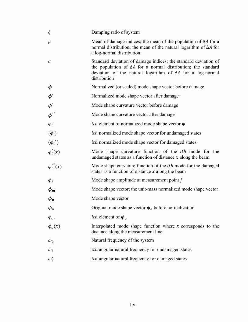
liv
Damping ratio of system
Mean of damage indices; the mean of the population of ∆ for a normal distribution; the mean of the natural logarithm of ∆ for a log-normal distribution
Standard deviation of damage indices; the standard deviation of the population of ∆ for a normal distribution; the standard deviation of the natural logarithm of ∆ for a log-normal distribution
Normalized (or scaled) mode shape vector before damage
∗ Normalized mode shape vector after damage
" Mode shape curvature vector before damage
"∗ Mode shape curvature vector after damage
element of normalized mode shape vector
normalized mode shape vector for undamaged states
∗ normalized mode shape vector for damaged states
" Mode shape curvature function of the mode for the undamaged states as a function of distance along the beam
"∗ Mode shape curvature function of the mode for the damaged states as a function of distance along the beam
Mode shape amplitude at measurement point
Mode shape vector; the unit-mass normalized mode shape vector
Mode shape vector
Original mode shape vector before normalization
element of
Interpolated mode shape function where corresponds to the distance along the measurement line
Natural frequency of the system
angular natural frequency for undamaged states
∗ angular natural frequency for damaged states

lv
LIST OF ABBREVIATIONS
2D Two Dimensional
3D Three Dimensional
ADC Analogue-to-Digital Converter
ANPSD Averaged Normalized Power Spectral Densities
ASTM American Standards for Testing and Materials
Avg. Average
C.O.V. Coefficient of Variation
CFRP Carbon Fibre Reinforced Polymer
CMIF Complex Mode Identification Function
COMAC Coordinate Modal Assurance Criterion
CPS Cross Power Spectrum
DAQ Data Acquisition
DC Direct Current
DFT Discrete Fourier Transform
DOF Degree of Freedom
ERA Eigen Realisation Algorithm
FE Finite Element
FFT Fast Fourier Transform
FRF Frequency Response Function
FRFs Frequency Response Functions
FT Fourier Transform
LabView Laboratory Virtual Instrumentation Engineering Workbench
LDT Linear Displacement Transducers
MAC Modal Assurance Criterion
MACEC A Matlab Toolbox for Experimental and Operational Modal Analysis
NDE Non-Destructive Evaluation

lvi
NExT Natural Excitation Technique
NI National Instruments
PCMCIA Peripheral Component Micro-Channel Interconnect Architecture
PP Peak Picking Method
R.R.S.D. Regular Residual Standard Deviation
S.S.R. Sum of Square of the Residuals
SHM Structural Health Monitoring
SPICE A Matlab Toolbox for Experimental and Operational Modal Analysis
SSH Simultaneous Sample and Hold
SSI Stochastic Subspace Identification
STDEV Standard Deviation
VBDD Vibration-Based Damage Detection
VBDI Vibration-Based Damage Identification
W.R.S.D. Weighted Residual Standard Deviation

1
CHAPTER 1. INTRODUCTION
1.1 Background
Due to the aging of materials, environment-related corrosion, overuse, overloading, and
an absence of sufficient maintenance, the existing inventory of bridges world-wide
continues to experience structural degradation. There are numerous reports about the
rapid deterioration of bridges. The majority of highway bridges in Japan are close to the
end of their design lives since most were built directly after World War II (Shrive 2005,
based on the work of Rahman 2000). Around 40% of all bridges in the United States
urgently need to be strengthened, rehabilitated, or replaced to remain in service, and this
number increases by about 5000 bridges a year (Shrive 2005, based on the work of
Aktan and Farhey 1996). More than 40% of the bridges in service in Canada were built
over 30 years ago. Many of these bridges need extensive works of maintenance,
rehabilitation or reconstruction to remain in good condition (or health) (Mufti 2001,
ISIS Canada 2001). To manage the resulting requirements for maintenance,
rehabilitation or reconstruction in a rational manner, there is an increasing need for
effective structural health monitoring (SHM) of bridges.
However, bridges are generally inspected at intervals of two or more years, mainly
relying on visual inspection (Biswas et al. 1990). Thus, there is the possibility that the
bridges may deteriorate to unsafe conditions as a result of experiencing damage between
inspection intervals. Also, visual inspections alone have been proven to be highly
unreliable due to the fact that the inspections rely heavily on the inspector’s experience
and knowledge (FHWA 2001). As a result, additional health monitoring, or condition
assessment, techniques need to be investigated for further application.
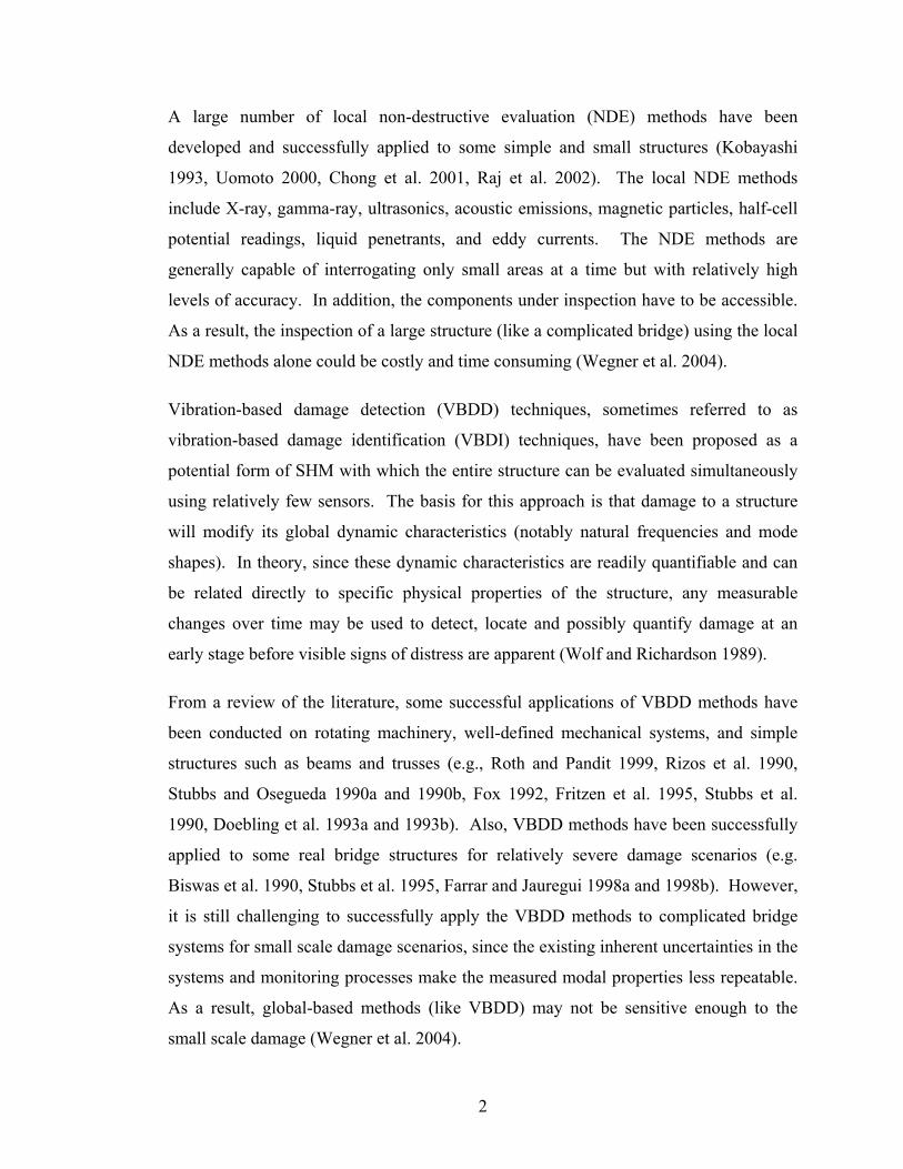
2
A large number of local non-destructive evaluation (NDE) methods have been
developed and successfully applied to some simple and small structures (Kobayashi
1993, Uomoto 2000, Chong et al. 2001, Raj et al. 2002). The local NDE methods
include X-ray, gamma-ray, ultrasonics, acoustic emissions, magnetic particles, half-cell
potential readings, liquid penetrants, and eddy currents. The NDE methods are
generally capable of interrogating only small areas at a time but with relatively high
levels of accuracy. In addition, the components under inspection have to be accessible.
As a result, the inspection of a large structure (like a complicated bridge) using the local
NDE methods alone could be costly and time consuming (Wegner et al. 2004).
Vibration-based damage detection (VBDD) techniques, sometimes referred to as
vibration-based damage identification (VBDI) techniques, have been proposed as a
potential form of SHM with which the entire structure can be evaluated simultaneously
using relatively few sensors. The basis for this approach is that damage to a structure
will modify its global dynamic characteristics (notably natural frequencies and mode
shapes). In theory, since these dynamic characteristics are readily quantifiable and can
be related directly to specific physical properties of the structure, any measurable
changes over time may be used to detect, locate and possibly quantify damage at an
early stage before visible signs of distress are apparent (Wolf and Richardson 1989).
From a review of the literature, some successful applications of VBDD methods have
been conducted on rotating machinery, well-defined mechanical systems, and simple
structures such as beams and trusses (e.g., Roth and Pandit 1999, Rizos et al. 1990,
Stubbs and Osegueda 1990a and 1990b, Fox 1992, Fritzen et al. 1995, Stubbs et al.
1990, Doebling et al. 1993a and 1993b). Also, VBDD methods have been successfully
applied to some real bridge structures for relatively severe damage scenarios (e.g.
Biswas et al. 1990, Stubbs et al. 1995, Farrar and Jauregui 1998a and 1998b). However,
it is still challenging to successfully apply the VBDD methods to complicated bridge
systems for small scale damage scenarios, since the existing inherent uncertainties in the
systems and monitoring processes make the measured modal properties less repeatable.
As a result, global-based methods (like VBDD) may not be sensitive enough to the
small scale damage (Wegner et al. 2004).
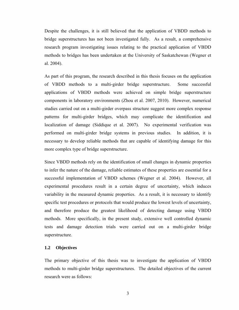
3
Despite the challenges, it is still believed that the application of VBDD methods to
bridge superstructures has not been investigated fully. As a result, a comprehensive
research program investigating issues relating to the practical application of VBDD
methods to bridges has been undertaken at the University of Saskatchewan (Wegner et
al. 2004).
As part of this program, the research described in this thesis focuses on the application
of VBDD methods to a multi-girder bridge superstructure. Some successful
applications of VBDD methods were achieved on simple bridge superstructure
components in laboratory environments (Zhou et al. 2007, 2010). However, numerical
studies carried out on a multi-girder overpass structure suggest more complex response
patterns for multi-girder bridges, which may complicate the identification and
localization of damage (Siddique et al. 2007). No experimental verification was
performed on multi-girder bridge systems in previous studies. In addition, it is
necessary to develop reliable methods that are capable of identifying damage for this
more complex type of bridge superstructure.
Since VBDD methods rely on the identification of small changes in dynamic properties
to infer the nature of the damage, reliable estimates of these properties are essential for a
successful implementation of VBDD schemes (Wegner et al. 2004). However, all
experimental procedures result in a certain degree of uncertainty, which induces
variability in the measured dynamic properties. As a result, it is necessary to identify
specific test procedures or protocols that would produce the lowest levels of uncertainty,
and therefore produce the greatest likelihood of detecting damage using VBDD
methods. More specifically, in the present study, extensive well controlled dynamic
tests and damage detection trials were carried out on a multi-girder bridge
superstructure.
1.2 Objectives
The primary objective of this thesis was to investigate the application of VBDD
methods to multi-girder bridge superstructures. The detailed objectives of the current
research were as follows:

4
to investigate the influence of various test parameters on the reliability and
repeatability of the measured dynamic properties (i.e., frequencies and mode
shapes) of a multi-girder bridge superstructure. Specifically, the issues
investigated included:
the influence of sensor types and locations, excitation types, sampling rates,
recording periods, and modal analysis methods on mode shape definition;
the influence of normalization methods on mode shape definition and
changes in mode shapes due to damage;
to develop appropriate damage detection techniques to identify the presence of
damage;
to define the damage detection resolutions of different test protocols based on
the statistical variability of the resulting damage indicator, and to use these to
identify the most appropriate test protocols;
to investigate the performance of the newly developed VBDD method on the
multi-girder bridge superstructure; and
to investigate patterns of damage induced changes across a spatially distributed
complex system (like a multi-girder bridge superstructure) using commonly
available VBDD indicators.
1.3 Contributions to Original Knowledge
A new Level 1 VBDD damage indicator was developed in this study. The resolutions of
different test protocols were defined based on the statistical characteristics of the new
damage indicator, as calculated both when there was no change in the condition of the
structure and when damage was present. The VBDD method, in combination with the
protocols identified as being most sensitive to damage, can be used effectively as the
initial component of a comprehensive SHM package for bridges by permitting a
relatively quick identification of the presence or absence of damage on the structure
with a high level of confidence.

5
It should be acknowledged that a VBDD damage indicator, called mode shape area
index, very similar to the one developed as part of this thesis work was found in the
literature during the later stages of preparation of this thesis (Huth et al. 2005).
However, the work presented in this thesis was developed independently and was
defined and applied in a different manner on a different application. In addition, the
application of the VBDD technique using a statistical approach is believed to be original.
A detailed comparison between two indicators is presented in Section 5.2.3.
The performance of the newly developed damage indictor was investigated on a multi-
girder bridge superstructure under well-controlled testing environments.
Also, five commonly used VBDD methods were applied on the complex, spatially
distributed multi-girder bridge superstructure system using well-controlled experimental
data.
1.4 Scope and Methodology
The current research focused primarily on the experimental application of vibration-
based damage detection on a multi-girder bridge superstructure. The structure used for
this investigation was a one-third scale model of a slab-on-girder composite bridge
superstructure featuring four steel girders supporting a steel-free concrete deck.
Constructed in the Structural Laboratory, University of Saskatchewan, the model was
based on a prototype superstructure forming part of the North Perimeter Red River
Bridge located in Winnipeg, Manitoba.
To facilitate the design and construction of the scaled bridge model, a preliminary field
test was conducted on the prototype bridge. Dimensions were measured and compared
with the as-built drawings. The dynamic properties (primarily the natural frequencies)
were measured using four accelerometers as the bridge was subjected to traffic
excitation forces.
Prior to carrying out the laboratory-based experimental test, a preliminary numerical
study was conducted to investigate the influence of several factors on the performance
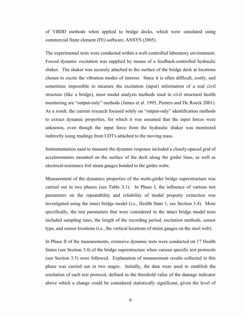
6
of VBDD methods when applied to bridge decks, which were simulated using
commercial finite element (FE) software, ANSYS (2005).
The experimental tests were conducted within a well-controlled laboratory environment.
Forced dynamic excitation was supplied by means of a feedback-controlled hydraulic
shaker. The shaker was securely attached to the surface of the bridge deck at locations
chosen to excite the vibration modes of interest. Since it is often difficult, costly, and
sometimes impossible to measure the excitation (input) information of a real civil
structure (like a bridge), most modal analysis methods used in civil structural health
monitoring are “output-only” methods (James et al. 1995, Peeters and De Roeck 2001).
As a result, the current research focused solely on “output-only” identification methods
to extract dynamic properties, for which it was assumed that the input forces were
unknown, even though the input force from the hydraulic shaker was monitored
indirectly using readings from LDT's attached to the moving mass.
Instrumentation used to measure the dynamic response included a closely-spaced grid of
accelerometers mounted on the surface of the deck along the girder lines, as well as
electrical-resistance foil strain gauges bonded to the girder webs.
Measurement of the dynamics properties of the multi-girder bridge superstructure was
carried out in two phases (see Table 3.1). In Phase I, the influence of various test
parameters on the repeatability and reliability of modal property extraction was
investigated using the intact bridge model (i.e., Health State 1, see Section 3.4). More
specifically, the test parameters that were considered in the intact bridge model tests
included sampling rates, the length of the recording period, excitation methods, sensor
type, and sensor locations (i.e., the vertical locations of strain gauges on the steel web).
In Phase II of the measurements, extensive dynamic tests were conducted on 17 Health
States (see Section 3.4) of the bridge superstructure when various specific test protocols
(see Section 3.5) were followed. Explanation of measurement results collected in this
phase was carried out in two stages. Initially, the data were used to establish the
resolution of each test protocol, defined as the threshold value of the damage indicator
above which a change could be considered statistically significant, given the level of

7
uncertainty. Subsequently, the performance of selected VBDD indicators was
investigated on the bridge superstructure under the 17 Health States.
1.5 Layout of the Thesis
The thesis is organized in seven chapters, with additional information provided in the
appendices. An overview of each chapter is described below.
Chapter 1 presents an overview of the research background, showing the need for
structural health monitoring and VBDD. The objectives, scope, and methodology are
also presented in the chapter. In addition, contributions to original knowledge are
identified.
In Chapter 2, a literature review, including an overview of the theoretical background of
SHM and VBDD, dynamic testing methods, and signal processing methods, is
presented.
The experimental program is described in Chapter 3, including descriptions of the
bridge model, the measurement of dynamic properties, data processing, and damage
cases considered.
Chapter 4 focuses on the evaluation of extracted dynamic properties and the influence of
test parameters on dynamic properties.
In Chapter 5, a new Level 1 VBDD indicator is presented. The development of the
damage indicator is described, and verification of the indicator using data from a FE
model is presented.
Chapter 6 presents the application of the newly developed damage indicator to the
model bridge superstructure. Specifically, a procedure used to define the resolution of a
specific test protocol is described. The results of threshold values for different test
procedures are presented. Detailed results of the application of the damage indicator to
the bridge are presented for the various damage cases considered. Also discussed in this
chapter is the performance of five commonly used VBDD methods when applied to the
multi-girder bridge for the damage cases considered.

8
Chapter 7 presents a summary and conclusions, as well as recommendations for future
research.
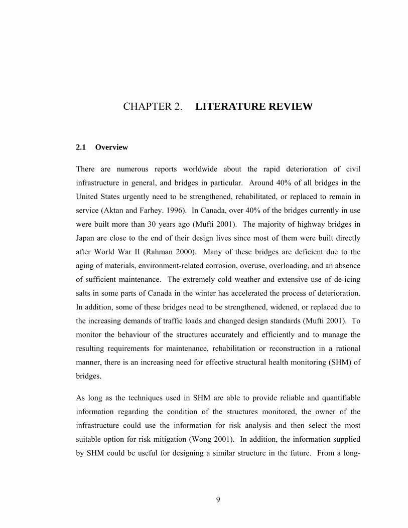
9
CHAPTER 2. LITERATURE REVIEW
2.1 Overview
There are numerous reports worldwide about the rapid deterioration of civil
infrastructure in general, and bridges in particular. Around 40% of all bridges in the
United States urgently need to be strengthened, rehabilitated, or replaced to remain in
service (Aktan and Farhey. 1996). In Canada, over 40% of the bridges currently in use
were built more than 30 years ago (Mufti 2001). The majority of highway bridges in
Japan are close to the end of their design lives since most of them were built directly
after World War II (Rahman 2000). Many of these bridges are deficient due to the
aging of materials, environment-related corrosion, overuse, overloading, and an absence
of sufficient maintenance. The extremely cold weather and extensive use of de-icing
salts in some parts of Canada in the winter has accelerated the process of deterioration.
In addition, some of these bridges need to be strengthened, widened, or replaced due to
the increasing demands of traffic loads and changed design standards (Mufti 2001). To
monitor the behaviour of the structures accurately and efficiently and to manage the
resulting requirements for maintenance, rehabilitation or reconstruction in a rational
manner, there is an increasing need for effective structural health monitoring (SHM) of
bridges.
As long as the techniques used in SHM are able to provide reliable and quantifiable
information regarding the condition of the structures monitored, the owner of the
infrastructure could use the information for risk analysis and then select the most
suitable option for risk mitigation (Wong 2001). In addition, the information supplied
by SHM could be useful for designing a similar structure in the future. From a long-

10
term point of view, it could reduce the life cycle costs of the infrastructure by providing
either a continuous or periodic indication of structural health (Mufti et al. 2005).
There are a large number of SHM techniques available, which include visual
inspections, local non-destructive evaluation (NDE) techniques such as X-ray, gamma-
ray, ultrasonics, acoustic emissions, magnetic particles, half-cell potential readings,
liquid penetrants, and eddy currents (e.g., Kobayashi 1993, Uomoto 2000, Chong et al.
2001, Raj et al. 2002), and global-based methods which use changes in the global
response of a structure to evaluate the health or condition of the structure (e.g., Pandey
et al. 1991, Fox 1992, Srinivasan and Kot 1992, Salawu and Williams 1994, and Zhang
and Aktan 1995). Although the local NDE methods are generally capable of
characterizing damage on a structure with relatively higher accuracy compared with
other methods, the inspection of a large structure (like a complicated bridge) using NDE
methods alone could be costly and time consuming (Wegner et al. 2004). This
observation has led to further investigation of effective global-based SHM methods.
Vibration-based damage detection (VBDD) techniques, a set of global SHM techniques,
have the potential to evaluate an entire structure simultaneously using relatively few
sensors. The basis for this approach is that damage to a structure will modify its global
dynamic characteristics (notably natural frequencies and mode shapes). In theory, since
these dynamic characteristics are readily quantifiable and can be related directly to
specific physical properties of the structure, any measurable changes over time may be
used to detect, locate and possibly quantify damage at an early stage before visible signs
of distress are apparent (Wolf and Richardson 1989). Although it is simple in concept,
extensive research is still required before VBDD methods can be applied reliably to
complex structures like bridges with multiple girders and spans. While quite a large
number of VBDD methods have been developed and successfully applied on some
simple structures, it is still a significant challenge to successfully apply VBDD methods
to real, large civil engineering structures (Wegner et al. 2004).
As a result, the primary objective of the current research is to investigate the application
of VBDD methods to multi-girder bridge superstructures. Specifically, in this chapter,
11
several of the main aspects of VBDD-related issues are reviewed and discussed. Firstly,
a broad overview of damage detection related issues are provided. To effectively
evaluate the condition of a structure based on its dynamic properties, it is important to
estimate or measure the modal properties of the structure with a high level of reliability
and confidence. It is therefore necessary to find a set of dynamic test procedures and
data processing methods which are suitable for the purpose of VBDD. As a result,
dynamic testing related issues and modal analysis methods are reviewed and discussed
based on the literature. Some commonly used VBDD methods are also reviewed in this
chapter, followed by a review of the application of VBDD methods to bridges. In the
final section of this chapter, a brief review of the VBDD related research conducted at
the University of Saskatchewan is provided.
2.2 Damage Detection
Damage (or fault) detection refers to the identification of a change in the performance of
a system compared with a previous, desired level of performance of the system using a
structural health monitoring process (Doebling et al. 1996). The previously existing,
desired level of performance serves as a reference point to define the state of health (or
damage) at some future time. Damage to a structure could include any of the following,
acting either individually or in combination: deteriorated material properties, changes in
physical and boundary conditions, lack of integrity in connections, and large
deformations in geometry. The damage can occur due to the aging of materials,
environment-related corrosion, overuse, overload, and an absence of sufficient
maintenance. Also, damage can occur suddenly due to unusual natural forces (like an
earthquake) and unexpected activities (like an impact force from a collision) (Farrar and
Doebling 1997).
Current damage detection methods applied to large civil engineering structures, like
bridges, are either visual or local non-destructive evaluation (NDE) methods (Biswas et
al. 1990). Visual inspections rely heavily on the inspector’s experience and knowledge,
which have been shown to be highly unreliable (FHWA 2001). The local NDE methods
can be applied to only small areas at a time. In practice, for assessing a larger system,

12
the local techniques require that the vicinity of the possible damage is known ahead of
time and that the components under inspection are accessible. Subjected to these
limitations, use of the local methods alone usually can only detect damage on or near the
surface of a large structure and the inspection could be costly and time consuming
(Wegner et al. 2004). Although the local NDE methods are generally capable of
detecting damage with higher accuracy compared with other methods, and are capable
of quantifying the extent of damage, no detailed review and discussion will be provided
here due to the limitations of the methods stated above. This research focused on the
global damage detection approach, specifically vibration-based damage detection
(VBDD) methods.
VBDD methods have received considerable attention in the literature. The basic idea
for these methods is that damage to a structure will modify its global dynamic
characteristics (notably natural frequencies and mode shapes). In theory, since these
dynamic characteristics are readily quantifiable and can be related directly to specific
physical properties of the structure, any measurable changes over time may be used to
detect, locate and possibly quantify damage at an early stage before visible signs of
distress are apparent. There are numerous VBDD methods proposed in the literature
which will be reviewed in detail in Section 2.5.
Rytter (1993) classified the damage detection methods into the following four
categories:
Level 1: Determination of the presence of damage in a structure;
Level 2: Determination of the location of damage in the structure, in addition to
Level 1;
Level 3: Quantification of the severity of the damage, in addition to Level 1 and
2; and
Level 4: Prediction of the remaining service life of the structure, in addition to
Level 1, 2, and 3.

13
The ultimate goal of structural health monitoring is that a set of damage detection
procedures is developed that is able to detect the presence of damage at a very early
stage, locate the damage within acceptable resolution, estimate the severity of the
damage, and predict the remaining useful life of the structure (Doebling et al. 1996).
However, only Level 1 and Level 2 methods (i.e., determination of the presence and
location of damage) will be investigated in this research.
The application of VBDD methods is very broad and has experienced a degree of
success in some areas, such as when applied to simple structural members (e.g Rizos et
al. 1990, Stubbs and Osegueda 1990b, Fox 1992, Fritzen et al. 1995, Stubbs et al. 1990,
Doebling et al. 1993a and 1993b), to shells and frames (e.g. Friswell et al. 1994, Nwosu
et al. 1995, Saitoh and Takei 1996), to aerospace structures (e.g., Hunt et al. 1990,
Grygier 1994, Doebling 1995), to offshore platforms (e.g., Yang, et al. 1984, Swamidas
and Chen 1992), to rotating machinery (e.g., Roth and Pandit 1999), to bridges (e.g.
Biswas et al. 1990, Stubbs et al. 1995, Farrar and Jauregui 1998a and 1998b), and to
other civil engineering structures (e.g. Salawu 1994, Skjaerbaek et al. 1996). However,
this research only focused on the application VBDD methods to bridges. A summary of
the literature on this application is provided in Section 2.6.
2.3 Dynamic Tests
2.3.1 Overview
One of the major topics of this research is vibration-based damage detection. The
success of the application of VBDD methods depends strongly on the quality of the
measured dynamic properties of the structure investigated. A set of proper dynamic
testing procedures is essential for the reliable estimation of the properties of the system.
To make a system vibrate with a certain energy level, and to keep it vibrating, the
system must be excited using external forces, which may include random environmental
excitation and forced excitation. To effectively collect and record the vibration response
in order to infer the modal properties of the system, a set of sensors is necessary for the
dynamic tests. In addition, uncertainties inherent in the test procedures lead to
14
variability, to some extent, in the measured modal properties between different test
trials. As a result, issues related to dynamic testing are addressed in this section.
2.3.2 Dynamic excitation
Excitation methods include the two general categories of ambient excitation (such as
traffic loading and wind loading) and forced excitation. Forced excitation may be
achieved by using a shaker (Biswas et al. 1990, Peeters and de Roeck 2000), impact
hammer (Samman and Biswas 1994), and drop weights (Peeters and de Roeck 2000).
From the literature review, it was found that random excitation appeared to be less
reliable for VBDD than harmonic loading (Zhou et al. 2005). Also, one advantage of
the forced vibration test is that the input force is typically strong enough to dominate
other noise disturbances, resulting in a strong signal to noise ratio, so that more reliable
measurements can be expected (Sohn et al. 2003). However, for online, real-time SHM,
the use of ambient excitation provides an attractive means of exciting field bridges since
the ambient traffic excitation is the most readily available source in field bridge
vibration tests. As a result, ambient excitation must be explored fully, as well as forced
excitation. Furthermore, it was found that the ambient vibration data provided adequate
estimates of the modal frequencies and modal damping ratios (Farrar and Cone 1995).
Similar conclusions were presented by Peeters and de Roeck (2000), who also found
that ambient excitation gave comparable results with much less cost. As a result, both
white noise random excitation and forced harmonic excitation were adopted and
investigated in this research.
2.3.3 Sensors
Accelerometers, strain gauges, anemometers, temperature sensors, and displacement
transducers were among the types of instrumentation cited in the literature.
Anemometers and temperature sensors were used to quantify the environmental
conditions, which is important for distinguishing the environmental influence on
structural dynamic properties. Strain gauges were employed in cable-supported bridges
15
to monitor the vertical bending, horizontal bending, torsion, vertical shear force, and
longitudinal compression forces (Ko et al. 1999).
In the laboratory, both accelerometers and strain gauges have been found to be capable
of generating data that can be used for VBDD purposes, although higher amplitude
forced vibrations are required to generate strain signals with sufficient magnitudes. In
addition, the bending curvature, which can be used for damage identification, can be
directly collected by bonding strain gauges to girder webs in vertically aligned groups
(Zhou et al. 2003). As a result, the more economically attractive strain gauges should be
investigated fully, as well as accelerometers (Wegner et al. 2004). Also, it has been
found that the number and configuration of sensors significantly influence the accuracy
of damage detection (Siddique et al. 2005).
2.3.4 Noise and uncertainty in dynamic tests
Ideally, two independent measurements of modal properties for a structure in the same
health state (or condition) would result in identical measured results. However,
practically, the measured modal properties obtained from different data sets in the same
health state always experienced variability due to the uncertainties inherent in the test
procedures. The uncertainties may be due to random noise, errors in sensor readings,
and disturbances of the input data during the data processing. Therefore, it is necessary
to investigate the influence of uncertainties on the performance of VBDD methods and
to evaluate the reliability of the measured modal properties in a statistical manner.
There were some investigations and statements related to the uncertainty issue available
in the literature.
Kim and Stubbs (1995) investigated the influence of uncertainties in measured modal
properties on the performance of vibration-based damage detection applied to a plate
girder model. The uncertainties considered in this research included different FE
models used to approximate the response of the plate girder, different estimation
methods used to calculate the stiffness parameters, and different methods used in the
definition of mode shapes. It was concluded that the uncertainties in measured modal
16
properties, especially the uncertainty in mode shape definition, had a great influence on
the accuracy of damage detection.
Alampalli et al. (1997) investigated the feasibility of using measured modal properties to
detect damage on a one-sixth scale steel-girder bridge model, as well as on a field
bridge. This research evaluated the influence of the uncertainty in the measured modal
properties on damage detection based on the calculated statistical parameters of the
modal properties. The damage detection methods used in this research included change
in natural frequencies, change in modal amplitudes, and change in Modal Assurance
Criterion (MAC) and Coordinate Modal Assurance Criterion (COMAC) values. It was
concluded that the damage indicators were not sensitive enough to detect the damage
when uncertainties (or random variation) were considered in the process.
Farrar and Doebling (1997), and Kirkegaard and Andersen (1998), stated in their
literature reviews that using statistical information of the measured modal properties is a
key issue for successful application of VBDD methods to civil engineering structures;
however, at that time, there was very little research investigating the application of
VBDD methods in a statistical manner.
Doebling et al. (1997) investigated the influence of the uncertainty of measured modal
properties on the performance of damage detection on a bridge structure excited by
impact forces. Monte Carlo simulations applied to the Frequency Response Function
(FRF) were used to calculate the uncertainties of the measured natural frequencies,
modes shapes and mode shape curvatures. It was concluded that, to detect the damage
using the VBDD methods, the measured modal properties had to experience some
changes, and the changes had to be statistically significant.
Doebling and Farrar (1998) investigated the application of VBDD methods on the I-40
Bridge, located in New Mexico, in a statistical manner. The researchers assumed that
the calculated modal properties of the FRF data followed a normal probability
distribution. In this manner, the statistical significance of changes in damage detection
indicators was evaluated. It was concluded that the changes in both modal properties
17
and damage indicators were statistically significant, which means that the damage could
be detected with a certain statistical confidence level.
2.4 Signal Processing and Modal Analysis
2.4.1 Overview
The performance of VBDD methods directly depends on the accuracy of measured
modal properties of structures investigated. It is essential to obtain reliable modal
properties since small-scale damage has been found to cause very small changes to
mode shapes and natural frequencies (Zhou et al. 2005, 2007). There are two general
steps required to reach this goal. The first step is to accurately acquire the dynamic
response through suitable vibration test protocols, as discussed in Section 2.3. The
second step is to process the collected vibration data to extract reliable modal properties
through suitable signal pre-processing techniques and post-processing modal analysis
methods.
Due to the imperfections inherent in practical dynamic testing systems, there are
unavoidable linear trends and/or noise combined into the actual response data. Also, it
is impossible to record data with absolute continuity in an infinitely long sampling
period, no matter how advanced the system is. To minimize the influence of these
factors on the measured modal properties, it is necessary to perform pre-processing on
the recorded data. Pre-processing techniques include functions to remove the initial
average baseline and linear trends, low-pass filters to reduce random noise, and window
functions to minimize the “leakage” of signals (Maia and Silva 1997).
Modal analysis is a post-processing method that extracts the modal properties of a
structure (i.e., natural frequencies, mode shapes, and damping ratios) through processing
of the recorded dynamic response of the structure (Ewins 2000). Traditional modal
analysis methods require both input (excitation forces) and output (vibration response)
information to estimate the modal properties of a structure; however, it is often difficult,
costly, and sometimes impossible to measure the excitation (input) information of a real
structure (like a bridge). As a result, most modal analysis methods used in civil
18
structural health monitoring are “output-only” methods, which assume the excitation
force to be white noise with a uniform spectrum in the frequency range of interest
(James et al. 1995, Peeters and De Roeck 2001). Generally, modal analysis methods
can be classified as frequency domain methods and time domain methods, depending on
whether frequency transform functions are used for the analysis (Maia and Silva 1997).
2.4.2 Frequency domain modal analysis methods
Frequency domain methods are modal analysis methods which extract the modal
properties based on the frequency response spectra obtained by transforming the signals
measured in the time domain. The most commonly used transform function is the Fast
Fourier Transform (FFT), which is an algorithm for computing the Discrete Fourier
Transform (DFT), a special Fourier Transform (FT) for discrete signals recorded
through a data acquisition system. The FFT is able to quickly transform data from the
time domain to the frequency domain using the periodicities of sinusoidal functions. In
this way, the FFT can analyze large amounts of waveform samples in much less time,
compared with the traditional Fourier transform process (Ramirez 1985).
Some commonly cited frequency domain methods in the literature included the Peak
Picking (PP) Method (Bendat and Piersol 1993), the Cross-Power Spectrum (CPS)
(James et al. 1995, Herman and Van Der Auweraer 1999, Farrar et al. 2000), Averaged
Normalized Power Spectral Densities (ANPSD) (Felber 1993), and Complex Mode
Indication Function (CMIF) methods (Shih et al. 1988, Brickner et al. 2000). Among
the methods, the Pick Picking (PP) method is the most widely used modal analysis
method in civil engineering, due mainly to the fact that it is the most simple and
straightforward method in both concept and practice. The PP method can be used to
identify the natural frequencies of a structure by picking the peaks in the response
spectra of the structure investigated. A detailed discussion of this method is presented
in the following paragraphs.
The dynamic response of a structure to an excitation force depends on both the
characteristics of the excitation force (mainly its amplitudes and frequency content) and
the inherent properties of the structure (mainly the distribution of its mass and stiffness).
19
For a single degree of freedom system, the displacement response spectrum of the
system, , can be defined as (Clough and Penzien 1975, 2003)
∙ [2.1]
where ω is the frequency of the excitation force, is the complex dynamic
amplification factor of the system, and is the Fourier transform (FT) of the
excitation force. The well-known magnitude of the amplification factor is defined as
| | [2.2]
where , , and are the frequency of the excitation force, the natural frequency of
the system, and the damping ratio of system (i.e., the ratio of damping coefficient to the
critical damping of the system; a dimensionless measure describing how oscillations in a
system decay after a disturbance), respectively. The dynamic amplification factor
for different damping ratios is plotted in the Figure 2.1. It can be seen from this figure
that the amplification factor reaches a peak when the frequency of the excitation force is
close to the natural frequency of the system, which is referred to as resonance; the
amplification factor becomes especially large for lower damping cases. For structures in
civil engineering, damping ratios usually vary from 0.5% to 2%, depending on the
material and connection types used in the system. As a result, at the peak in the
magnification function, the difference between the natural frequency and the excitation
frequency is less than 1%. In this manner, the frequency at the peak location in the plot
of the displacement response spectrum of the system, , can be referred to as the
damped natural frequency (very close to the un-damped natural frequency for civil
engineering structures), as long as the excitation force approximates white noise with a
flat spectrum (i.e., a force with equal energy content at all frequencies in the frequency
range of interest).
A similar situation exists for multiple degree of freedom systems, for which there are
multiple peaks in the Frequency Response Function (FRF) (one peak for each degree of
freedom (DOF); i.e., there is one possible mode for each DOF). As a result, the PP
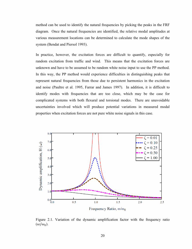
20
method can be used to identify the natural frequencies by picking the peaks in the FRF
diagram. Once the natural frequencies are identified, the relative modal amplitudes at
various measurement locations can be determined to calculate the mode shapes of the
system (Bendat and Piersol 1993).
In practice, however, the excitation forces are difficult to quantify, especially for
random excitation from traffic and wind. This means that the excitation forces are
unknown and have to be assumed to be random white noise input to use the PP method.
In this way, the PP method would experience difficulties in distinguishing peaks that
represent natural frequencies from those due to persistent harmonics in the excitation
and noise (Paultre et al. 1995, Farrar and James 1997). In addition, it is difficult to
identify modes with frequencies that are too close, which may be the case for
complicated systems with both flexural and torsional modes. There are unavoidable
uncertainties involved which will produce potential variations in measured modal
properties when excitation forces are not pure white noise signals in this case.
Figure 2.1. Variation of the dynamic amplification factor with the frequency ratio ( / ).

21
2.4.3 Time domain modal analysis methods
Time domain methods are modal analysis methods which can extract the modal
properties directly from the recorded data in the time domain (i.e., no Fourier transform
is required). Less commonly, time domain methods may use time history data which
have been transformed from the measured (or recorded) frequency spectra using inverse
Fourier transforms (Maia and Silva 1997).
Some commonly cited time domain methods in the literature include the Eigen
Realisation Algorithm (ERA) method (Juang and Papa 1985), the Natural Excitation
Technique (NExT) (James et al. 1992, 1995), the Stochastic Subspace Identification
(SSI) method (Van Overschee and De Moor 1996, Peeters and De Roeck 2001), and
some other methods based on the SSI method.
The Eigen Realisation Algorithm (ERA) method can be used to identify the modal
properties of a structure through realizing the state-space system which is built based on
the recorded vibration data. The state-space system is the representation of a physical
system through a set of first-order differential equations with variables including input
(measured or assumed excitation forces) and output (recorded displacement or
acceleration response) information. The modal properties (eigenvalues and
eigenvectors) are extracted from the realized state-space matrices by processing the
equations in the time domain.
Stochastic Subspace Identification (SSI) is a time domain method which can extract the
modal properties of a system by identifying a stochastic state-space model from a
system with unknown ambient input excitation forces, and only available output
measurements. The state model deals with linear vibration systems excited by a
stochastic process (white noise), which makes the SSI method much faster and more
robust than some nonlinear system-based methods like the Prediction Error Method
(Ljung 1987), even though it is somewhat slower than the frequency domain-based PP
method (Peeters and De Roeck 2001).

22
The dynamic behaviour of a structure with discrete masses connected through springs
and dampers can be defined by the following second-order differential matrix equation:
[2.3]
where , , and are the mass, damping and stiffness matrices, respectively; is
the displacement vector; is the excitation force vector; and and are the
second and first derivatives, respectively, of the displacement with respect to continuous
time. For a system with distributed or continuous mass, finite element methods can be
used to discretize the system first, so that the same equation applies. Practically, to
describe structures in civil engineering (like bridges), Equation 2.3 needs to be
converted to a more suitable form to represent the discrete-time stochastic state model,
which is based on the practical situation that only a few measurement points are usually
selected (instead of measurements of all degrees of freedom), that the data are sampled
at discrete time intervals, that no excitation forces are usually measured, and that there
are measurement and process noise involved in the data.
Peeters and De Roeck (1998) converted Equation 2.3 into the following simplified
forms:
[2.4a]
[2.4b]
where is the state matrix which represents the dynamic properties of the system; is
the output matrix which refers to how system states are transformed to the output
(response) of the system; is the state vector with elements that independently
describe the state of the system; is the output vector at discrete time interval ;
and are the process noise due to disturbances of input data and the measurement
noise due to the inaccuracy of the data acquisition system, respectively. After the state-
space model of the structure is established, the model properties of the system can be
identified through an eigenvalue analysis.
23
2.5 VBDD Methods
2.5.1 Overview
Structural health monitoring (SHM) or condition assessments on structures (like
bridges) are generally carried out by visual inspection at intervals of two or more years
(Biswas et al. 1990). The visual inspections are highly subjective and rely heavily on
the inspector’s experience and knowledge, which makes the method unreliable if no
other methods are used in combination at the same time (FHWA 2001). As a result, a
large number of local non-destructive evaluation (NDE) methods have been developed
and applied successfully to some simple and small structures (Kobayashi 1993, Uomoto
2000, Chong et al. 2001, Raj et al. 2002). The NDE methods are generally capable of
assessing the condition of structures with relatively higher accuracy. However, the local
NDE methods can only examine a small area at a time. In addition, the components to
be inspected have to be accessible. As a result, the inspection of a large structure (like a
complicated bridge) using the NDE methods alone could be costly and time consuming
(Wegner et al. 2004). It is still important to look for other potential methods, like global
methods.
Numerous VBDD methods, a set of global methods, have been proposed as potential
forms of SHM, all related in some manner to changes in modal parameters (notably
natural frequencies, damping, and mode shapes). The methods are able to evaluate the
entire structure simultaneously using relatively few sensors. The basis for this approach
is that damage to a structure will modify its global dynamic characteristics. In theory,
since these dynamic characteristics are readily quantifiable and can be related directly to
specific physical properties of the structure, any measurable changes over time may be
used to detect, locate and possibly quantify damage at an early stage before visible signs
of distress are apparent (Wolf and Richardson 1989). Detailed literature reviews of
VBDD methods had been provided by Doebling et al. (1996, 1998) and Sohn et al.
(2003). A summary of the reviews is presented in the following paragraphs.
Changes in natural frequency have been investigated and cited by many researchers
(Loland and Dodds 1976, Cawley and Adams 1979, Doebling et at. 1996, Salawu 1997).
24
This method uses the changes in natural frequencies between two health states (or
conditions) of a structure to infer the presence of possible damage on the structure.
Theoretically, the stiffness of a structure decreases after damage occurs, which will
induce some decrease in the measured natural frequencies. In this manner, the changes
in the natural frequencies can be used to infer the presence of damage. Practically,
however, changes in frequency have been proven not to be sensitive enough to detect
small scale damage when considering the influence of temperature changes and other
environmental conditions (Doebling et al. 1996).
There is some research reported in the literature related to the use of damping for
damage assessment (Adams et al. 1975, Casas and Aparicio 1994, Salawu and Williams
1995, Kong et al. 1996, and Farrar and Jauregui 1998a), even though the amount of
damping-related literature is much more limited than that related to frequencies and
mode shapes. In general, it was found that the damage detection methods based on
damping are unreliable and not sensitive to small-scale damage due to the fact that the
accuracy of the measured damping from vibration tests is usually poor and there has not
been a consistent relationship observed between the measured damping and the damage
induced.
On the other hand, the VBDD methods based on mode shapes and their derivatives has
received considerable attention. Some of these methods have been successfully applied
to simple structures in the field, as well as some complex structures in simulation
(Pandey et al. 1991, Fox 1992, Srinivasan and Kot 1992, Salawu and Williams 1994,
and Zhang and Aktan 1995). There are several commonly cited VBDD methods based
on mode shapes and their derivatives, including changes in mode shape, changes in
mode shape curvature, changes in flexibility, changes in uniform flexibility curvature,
and the damage index method. These five VBDD methods will be discussed in detail in
the following sections. Also, the performance of the five VBDD methods on the multi-
girder bridge superstructure addressed in this research was investigated in Chapter 6.

25
2.5.2 Change in mode shape method
The change in mode shape method, as an indicator of damage, simply uses the
difference between the undamaged and damaged mode shapes. Due to its simplicity, the
change in mode shape method has received a large amount attention and has been cited
by many researchers (e.g., Mazurek and DeWolf 1990, Srinivasan and Kot 1992).
The method is defined as:
∆ ∗ [2.5]
in which, for each individual vibration mode, represents a normalized (or scaled)
mode shape vector before damage; ∗ is a normalized mode shape vector after damage;
therefore, ∆ represents the calculated change in mode shape vector.
The mode shapes, ∗ and , must be normalized (or scaled) to a common basis to allow
for meaningful comparisons due to the fact that the scale of mode shape amplitudes is
arbitrary. Siddique et al. (2007) found that near optimal normalization for VBDD was
achieved when mode shape vectors were scaled to have a unit norm, i.e., 1.
Various mode shape normalization schemes, and their effect on calculated mode shape
changes, are discussed in Chapter 4.
Since damage to a structure is expected to cause a localized decrease in stiffness, the
greatest change in the mode shape amplitude is expected to occur at the location of
damage. It should be mentioned that the change in mode shape method is able to detect
and localize the damage on the structure. Practically, however, the method alone has
difficulty in determining quantitatively whether or not damage is present. As a result, a
new Level 1 damage indicator (i.e., one capable of identifying the presence, but not
location, of damage) was developed based on the change in mode shape method. The
detailed information about this is presented in Chapter 5.

26
2.5.3 Damage index method
Stubbs et al. (1995) derived the damage index method to detect damage on a structure.
It is based on the change in the strain energy stored in a beam-like structure when it
deforms in one of its mode shapes. The damage index for the mode at location
on the beam can be defined in continuous form as
"∗ "∗
" "
"
"∗ [2.6]
in which " and "∗ are the mode shape curvature functions of the mode for
the undamaged and damaged states, respectively, as a function of distance along the
beam; represents the length of the beam; and and represent the limits of the
segment of the beam over which damage is being evaluated.
In discrete form, assuming that the spacing between measurement points in the mode
shape vectors is uniform, the damage index can be rewritten as:
" ∗ ∑ " ∗
" ∑ "
∑ "
∑ " ∗ [2.7]
in which is the number of locations where modal curvature is calculated along the
beam. Assuming that the set of damage indices for the beam forms a sample of a
normally distributed population, a normalized damage indicator then can be defined as:
/ 2.0 [2.8]
in which represents the normalized damage indicator; and represent the mean and
standard deviation of damage indices, respectively, for all locations considered.
Normalized damage indices falling two or more standard deviations from the mean are
expected to be indicative of the presence of damage and a possible damage location.
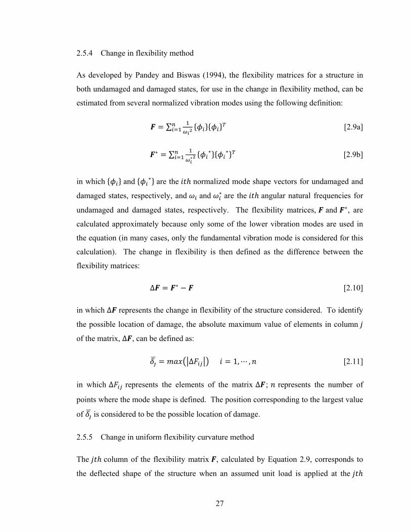
27
2.5.4 Change in flexibility method
As developed by Pandey and Biswas (1994), the flexibility matrices for a structure in
both undamaged and damaged states, for use in the change in flexibility method, can be
estimated from several normalized vibration modes using the following definition:
∑ [2.9a]
∗ ∑∗
∗ ∗ [2.9b]
in which and ∗ are the normalized mode shape vectors for undamaged and
damaged states, respectively, and and ∗ are the angular natural frequencies for
undamaged and damaged states, respectively. The flexibility matrices, and ∗, are
calculated approximately because only some of the lower vibration modes are used in
the equation (in many cases, only the fundamental vibration mode is considered for this
calculation). The change in flexibility is then defined as the difference between the
flexibility matrices:
∆ ∗ [2.10]
in which ∆ represents the change in flexibility of the structure considered. To identify
the possible location of damage, the absolute maximum value of elements in column
of the matrix, ∆ , can be defined as:
∆ 1,⋯ , [2.11]
in which ∆ represents the elements of the matrix ∆ ; represents the number of
points where the mode shape is defined. The position corresponding to the largest value
of is considered to be the possible location of damage.
2.5.5 Change in uniform flexibility curvature method
The column of the flexibility matrix , calculated by Equation 2.9, corresponds to
the deflected shape of the structure when an assumed unit load is applied at the
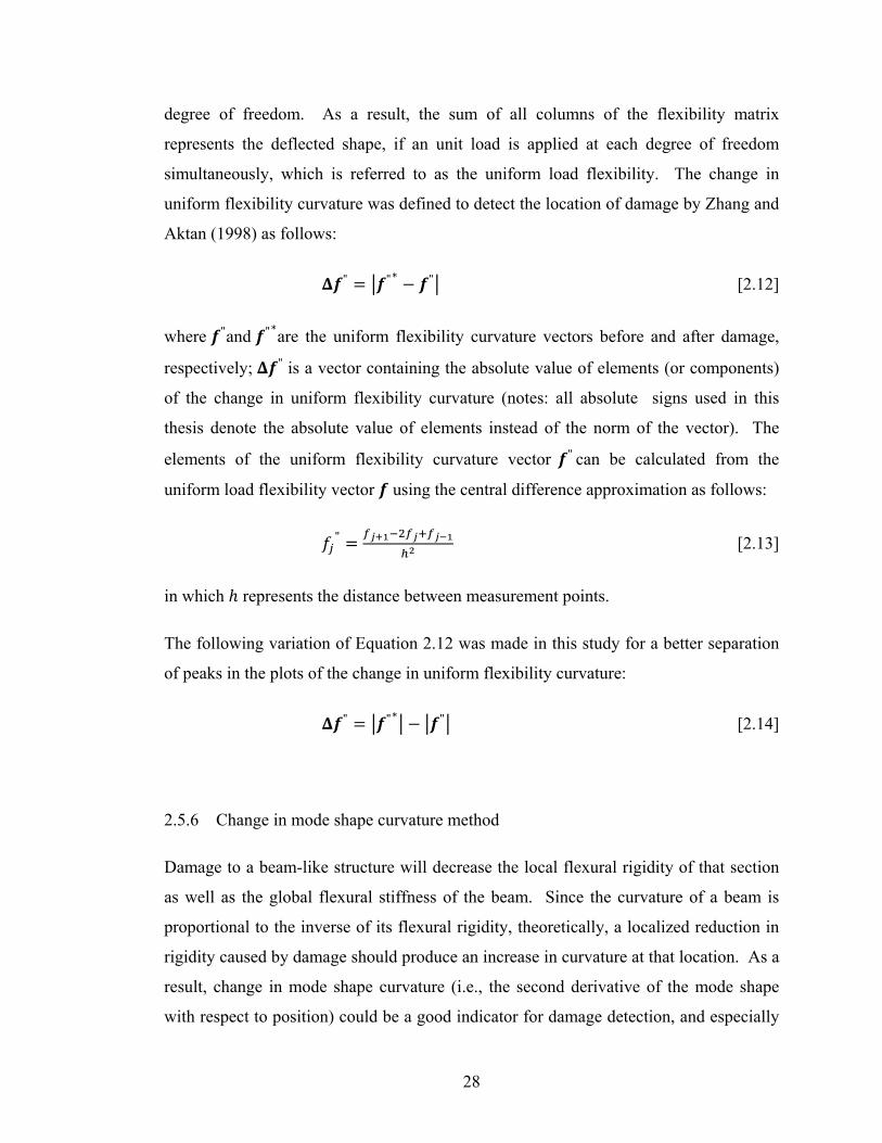
28
degree of freedom. As a result, the sum of all columns of the flexibility matrix
represents the deflected shape, if an unit load is applied at each degree of freedom
simultaneously, which is referred to as the uniform load flexibility. The change in
uniform flexibility curvature was defined to detect the location of damage by Zhang and
Aktan (1998) as follows:
" "∗ " [2.12]
where "and "∗are the uniform flexibility curvature vectors before and after damage,
respectively; " is a vector containing the absolute value of elements (or components)
of the change in uniform flexibility curvature (notes: all absolute signs used in this
thesis denote the absolute value of elements instead of the norm of the vector). The
elements of the uniform flexibility curvature vector " can be calculated from the
uniform load flexibility vector using the central difference approximation as follows:
" [2.13]
in which represents the distance between measurement points.
The following variation of Equation 2.12 was made in this study for a better separation
of peaks in the plots of the change in uniform flexibility curvature:
" "∗ " [2.14]
2.5.6 Change in mode shape curvature method
Damage to a beam-like structure will decrease the local flexural rigidity of that section
as well as the global flexural stiffness of the beam. Since the curvature of a beam is
proportional to the inverse of its flexural rigidity, theoretically, a localized reduction in
rigidity caused by damage should produce an increase in curvature at that location. As a
result, change in mode shape curvature (i.e., the second derivative of the mode shape
with respect to position) could be a good indicator for damage detection, and especially
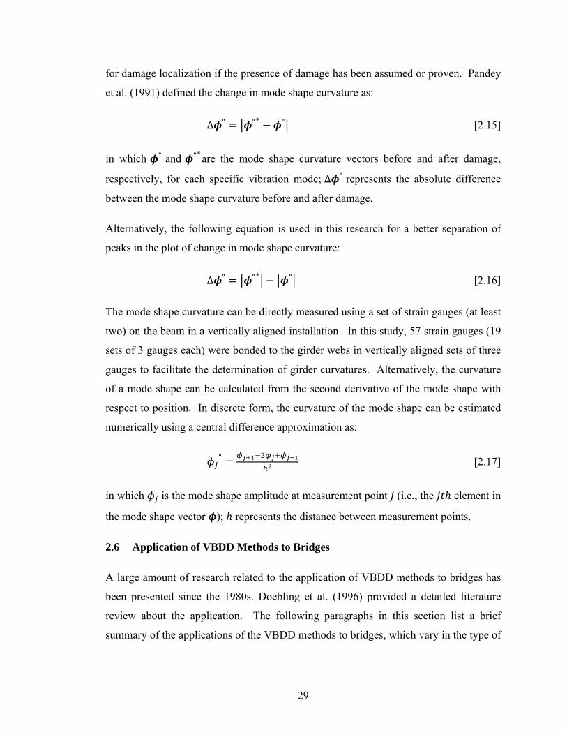
29
for damage localization if the presence of damage has been assumed or proven. Pandey
et al. (1991) defined the change in mode shape curvature as:
∆ " "∗ " [2.15]
in which " and "∗are the mode shape curvature vectors before and after damage,
respectively, for each specific vibration mode; ∆ " represents the absolute difference
between the mode shape curvature before and after damage.
Alternatively, the following equation is used in this research for a better separation of
peaks in the plot of change in mode shape curvature:
∆ " "∗ " [2.16]
The mode shape curvature can be directly measured using a set of strain gauges (at least
two) on the beam in a vertically aligned installation. In this study, 57 strain gauges (19
sets of 3 gauges each) were bonded to the girder webs in vertically aligned sets of three
gauges to facilitate the determination of girder curvatures. Alternatively, the curvature
of a mode shape can be calculated from the second derivative of the mode shape with
respect to position. In discrete form, the curvature of the mode shape can be estimated
numerically using a central difference approximation as:
" [2.17]
in which is the mode shape amplitude at measurement point (i.e., the element in
the mode shape vector ); represents the distance between measurement points.
2.6 Application of VBDD Methods to Bridges
A large amount of research related to the application of VBDD methods to bridges has
been presented since the 1980s. Doebling et al. (1996) provided a detailed literature
review about the application. The following paragraphs in this section list a brief
summary of the applications of the VBDD methods to bridges, which vary in the type of

30
bridge tested, excitation forces used, damage considered, and the VBDD methods
implemented.
Salane et al. (1981) investigated vibration-based damage detection on a three-span
highway bridge. The stiffness (directly related to the dynamic properties) of the bridge
was extracted from the experimental test data collected during a fatigue test. Excitation
forces were provided by an electro-hydraulic actuator. It was found that changes in
bridge stiffness and mechanical impedance plots could be used as a good indicator of
damage resulting from fatigue cracks.
Biswas et al. (1990) performed an investigation of VBDD on a two-span composite
highway bridge. Excitation forces were supplied by a shaker. Damage was simulated
by unfastening a set of bolts at a steel girder splice connection. Changes in frequency
response functions (FRFs) were found to be detectable and quantifiable. The natural
frequencies decreased consistently due to the incremental increase in damage, even
though the reduction was small.
Mazurek and DeWolf (1990) performed laboratory vibration tests on a two-span
aluminum plate-girder bridge model. Excitation was provided by a small scale vehicle
model. Damage was simulated by support failure and progressive cracking of the bridge
girder at mid-span. It was found that major structural deterioration can cause significant
changes to both natural frequencies and mode shapes. It was also shown that changes in
mode shapes can be used to locate the damage as long as the presence of the damage
had been identified.
Farrar et al. (1994) conducted vibration tests on the I-40 bridge over the Rio Grande,
located in Albuquerque, NM, to investigate the performance of several VBDD methods.
The bridge consisted of a concrete deck supported by two steel plate girders (a so-called
“fracture critical” design based on the fact that failure of either of the main girders is
assumed to produce catastrophic failure of the bridge). Damage was introduced to the
bridge by incrementally cutting through one of the main girders. The bridge was excited
using both ambient excitation (automobile traffic on the adjacent bridge) and a hydraulic
shaker. Accelerometers were used to measure the vibration response. In general, the

31
results indicated that natural frequency was not a sensitive indicator of damage.
However, the mode shape-related damage indicators, including the damage index, the
mode shape curvature, and change in flexibility, change in uniform flexibility curvature,
were shown to be more sensitive to the damage induced.
Farrar and Cone (1995) presented further analysis of the I-40 bridge damage detection
data described by Farrar et al. (1994). It was concluded that ambient excitation
provided a good estimate for the extracted natural frequencies for SHM while the
measured changes due to the damage in both natural frequencies and mode shapes were
not large enough to detect the damage at an early stage.
Stubbs et al. (1995) applied the damage index method to the I-40 bridge data (the same
bridge that was studied by Farrar and Cone 1995). The data was interpolated at 160
locations using a spline function before the application of the damage index method. It
was concluded that the method could locate the damage with an error (or the difference
between the actual and predicted damage location) of 2.5% of the span.
Wang et al. (1997) conducted an investigation of the damage index method on a scaled
simple span bridge model supported by plate girders. Excitation for the dynamic tests
was provided by an impact hammer applied at a fixed point. Damage was induced on
the girder flanges. The lowest six mode shapes were extracted from the measured
acceleration data. The normalized damage index was found to be sensitive to damage
for severe damage cases.
Farrar and Jauregui (1998a, 1998b) investigated the performance of five damage
detection methods on a three-span bridge, which consisted of a concrete deck supported
by two steel plate girders, using both experimental and numerical data. The VBDD
methods considered in this study included the damage index method, mode shape
curvature method, change in flexibility method, change in uniform load surface
curvature method, and change in stiffness method. Different severity levels of damage
were introduced to the bridge to investigate the performance of the selected VBDD
indicators. It was concluded that all methods could locate severe damage cases while
32
the performance of the methods varied for small scale damage cases. In general, the
damage index method performed best in most cases.
Using dynamic tests, Stubbs et al. (1999) investigated the performance of the damage
index method on a four lane highway bridge that crossed I-40. Both the natural
frequencies and mode shapes for the five lowest modes were extracted through the data
collected from the bridge in an already damaged state. A finite element (FE) model was
developed, which was based on the information from as-built drawings of the bridge, to
serve as a baseline (or pristine condition) reference. It was concluded that damage can
be detected by comparing the mode shapes of the real structure and the FE model. The
estimated damage locations using the damage index method showed a good correlation
with the observed cracking patterns.
Pearson et al. (2001) conducted experimental dynamic tests on a quarter-scale simply
supported concrete bridge deck supported by Tee beams. Accelerometers were used to
collect the vibration data while excitation was provided by an instrumented hammer.
Different severity levels of damage were considered on the bridge once the baseline
dynamic properties of the model had been established in the intact condition. Cracks
were induced by applying four point bending loads. It was found that changes in
dynamic properties for higher modes (mode 3 and above) were more sensitive to
damage than those for lower modes. It was also found that induced damage either
produced an entirely new vibration mode or changed the order of vibration modes.
Huth et al. (2005) performed large scale dynamic tests on a prestressed concrete
highway bridge to investigate the sensitivity of several damage detection methods using
measured modal properties. Output-only modal identification methods were used in this
research to extract modal properties. From the results of this research, it was found that
a change in natural frequencies may not be a sensitive indicator since the changes of
natural frequencies were minor even when severe cracks were introduced. A novel
damage indictor, called the mode shape area index was developed and found to be a
sensitive damage detection approach (it should be acknowledged that a similar VBDD
damage indicator, called the area of mode shape change, has been developed in this
33
thesis prior to finding this reference. However, the work presented in this thesis was
developed independently and was defined and applied in a different manner on a
different application. A detailed comparison between two indicators is presented in
Section 5.2.3).
Galvín and Domínguez (2007) conducted dynamic tests on the Barqueta Bridge, a cable
stayed bridge deck over the Guadalquivir River in Seville, Spain. The bridge was
excited using ambient traffic, and dynamic measurements were collected by
accelerometers. There was no significant change observed for damage indices between
two tests separated by an interval of one year; therefore, it was claimed that the structure
had no damage induced during the period. Vibration tests on a simpler laboratory model
showed that the damage index method could locate damage with an error of less than
3% of the span.
2.7 VBDD Research Conducted at the University of Saskatchewan
The research described in this thesis is part of a comprehensive program undertaken at
the University of Saskatchewan to investigate issues relating to the practical application
of VBDD methods to bridges. This comprehensive research program includes both
well-controlled experimental studies and field tests with various environmental
conditions, while both actual testing methods and numerical simulations were
considered (Wegner et al. 2004). The topics investigated in this comprehensive
program include the influence of sensor type and configuration on the performance of
VBDD, the influence of excitation sources on the structural health monitoring, a
comparison between different VBDD methods based on both experimental and
simulated vibration data, the influence of temperature on the measured modal properties,
and the influence of data processing (including normalization methods and interpolation
methods) on the performance of VBDD on the specific structures investigated (Wegner
et al. 2004). The following paragraphs list detailed descriptions and findings for the
specific topics.
Zhou et al. (2004 and 2010) investigated the performance of five VBDD techniques on
the damage detection of a full-scale pre-stressed concrete girder. The tests were

34
conducted under well-controlled laboratory environments. Damage cases considered
included the removal of small blocks of concrete from the surface of the concrete girder.
Both accelerometers and strain gauges were used to collect vibration response data. It
was found that as few as six accelerometers located along the span of the girder were
sufficient to detect and locate the damage, while only the fundamental mode shape was
used for this purpose. The accuracy of the damage detection depended on the spacing of
the sensors, the distance between sensors and the induced damage, and the location of
the damage relative to the supports. It was also found that the change in mode shape
method was the most reliable method to detect the damage.
Zhou et al. (2007) performed both numerical and experimental investigations on VBDD
of a scaled bridge deck model featuring two steel girders supporting a steel-free concrete
bridge deck, while the structure was simply supported. The performance of five
selected VBDD methods was investigated to detect and localize small-scale damage on
the deck. A small number of sensors including both accelerometers and strain gauges
were adopted in the well controlled experimental tests. The fundamental mode shape
alone was found to be sufficient to detect and locate the damage in this case, while
higher modes tended to be less reliable. It was found that damage could be detected and
localized using as few as five measurement points in the longitudinal direction of the
bridge with reasonable accuracy. The paper also stated that it was difficult to detect the
damage located near the supports.
Siddique et al. (2005, 2006, and 2007) performed both field tests and numerical studies
on the application of VBDD methods to a two-span, multi-girder, integral abutment
bridge in Saskatoon, Canada. From the field tests, it was found that the ambient
temperature significantly influenced the measured natural frequencies. A calibrated FE
model was used to evaluate the effect of sensor spacing, mode shape normalization, and
uncertainty on the performance of several selected VBDD methods. It was stated that
small-scale damage on the bridge deck could be detected and/or located if measurement
points were located close enough to the location of the damage. It was also concluded
that the reliability of the measured mode shapes could be improved by averaging the
repeated trials.
35
Pham et al. (2007) performed both field vibration tests and numerical studies on a two-
span integral abutment overpass, which was the same bridge investigated by Siddique et
al. (2007), located in Saskatoon, Canada. This study focused on the influence of
temperature variation on the dynamic properties of the overpass and the ability of
VBDD methods to detect and localize simulated damage. It was concluded that the
variation of ambient temperature affected the stiffness of the structure and therefore
changed the measured natural frequencies and mode shapes significantly. It was shown
that the natural frequencies for the three lowest modes increased when the temperature
decreased. It was also found that the patterns of mode shape changes caused by small-
scale damage were different from those due to temperature effects when a sufficient
number of measurement points was used and the measurement points were located close
to the simulated damage.
Alwash et al. (2005, 2006, and 2009) investigated several issues related to application of
VBDD in the structural health monitoring of bridges, but primarily focused on the
influence of the excitation sources on the performance of VBDD methods through both
experimental and numerical studies. The research was conducted on a three span
reinforced concrete bridge strengthened by the addition of external steel reinforcement
in regions of high positive moment. It was found that the characteristics of the
excitation sources had significant effects on the quality of modal properties extracted
from the dynamic response of the bridge. From the calibrated numerical model, it was
concluded that harmonic excitation, impact excitation, and free vibration after random
excitation was discontinued were consistent enough to be used to detect the simulated
damage. In the field tests, free vibration after the vehicle left the bridge generated the
most reliable modal properties. It was also stated that noise had a significant influence
on the performance of VBDD on bridges.
2.8 Summary
Numerous VBDD methods, a set of global methods, have been proposed as a potential
form of SHM, all related in some manner to changes in modal parameters (notably
natural frequencies, damping, and mode shapes). The methods are able to evaluate the

36
entire structure simultaneously using relatively few sensors. Although there were some
successful applications of the proposed VBDD methods, great challenges are still
apparent in the practical application of the methods to complicated structural systems
like bridges. As a result, the primary objective of the current research was to investigate
the application of VBDD methods to multi-girder bridge superstructures.
The performance of VBDD methods directly depends on the accuracy of measured
modal properties of structures investigated. It is essential to obtain reliable modal
properties since small-scale damage has been found to cause very small changes to
mode shapes and natural frequencies. As a result, a part of this research was designed to
investigate and quantify the influence of various test procedures on the reliability and
repeatability of the measured dynamic properties of the multi-girder bridge
superstructure through extensive dynamic tests.
From the literature review, it was found that the changes in natural frequencies have
proven not to be sensitive enough to detect small scale damage practically, especially
considering the experimental uncertainties like the influence of temperature changes and
other environmental conditions. In general, the damage detection methods based on
change in damping were found to be unreliable and not sensitive to small-scale damage
due to the fact that the accuracy of the measured damping from vibration tests is usually
poor and there is no consistent relationship between the measured damping and the
damage induced. The methods based on mode shapes and their derivatives, on the other
hand, appear to be a good source to seek a sensitive and effective damage indicator.
However, most of the proposed methods based on mode shapes have not really
answered the questions related to determining the presence of damage with a specific,
statistically-based level of confidence, which is generally acknowledged to be the most
effective approach for practical problems involving great uncertainties. This limitation
may be partially due to the fact that the definition of the mode shape, as it is commonly
performed, is not unique, making investigation of mode shapes in a statistical manner
more difficult. As a result, a new Level 1 VBDD indicator (i.e., one capable of
identifying the presence, but not location, of damage) was proposed in this research to
fill this gap.
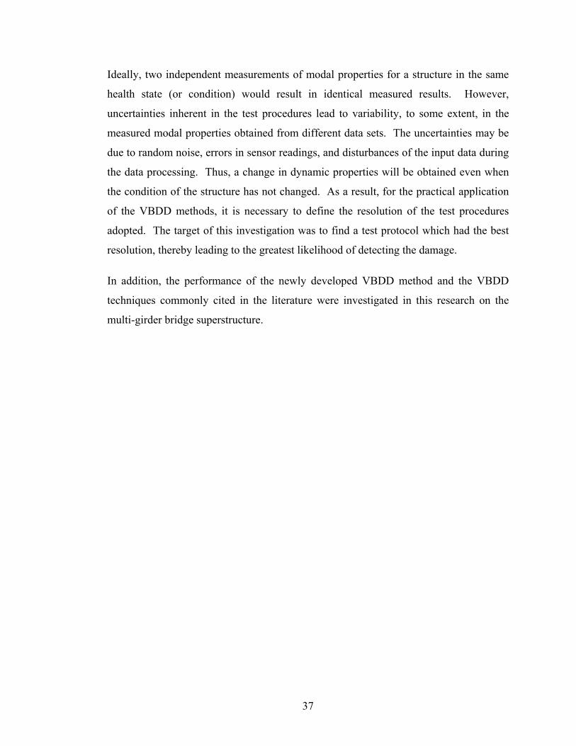
37
Ideally, two independent measurements of modal properties for a structure in the same
health state (or condition) would result in identical measured results. However,
uncertainties inherent in the test procedures lead to variability, to some extent, in the
measured modal properties obtained from different data sets. The uncertainties may be
due to random noise, errors in sensor readings, and disturbances of the input data during
the data processing. Thus, a change in dynamic properties will be obtained even when
the condition of the structure has not changed. As a result, for the practical application
of the VBDD methods, it is necessary to define the resolution of the test procedures
adopted. The target of this investigation was to find a test protocol which had the best
resolution, thereby leading to the greatest likelihood of detecting the damage.
In addition, the performance of the newly developed VBDD method and the VBDD
techniques commonly cited in the literature were investigated in this research on the
multi-girder bridge superstructure.
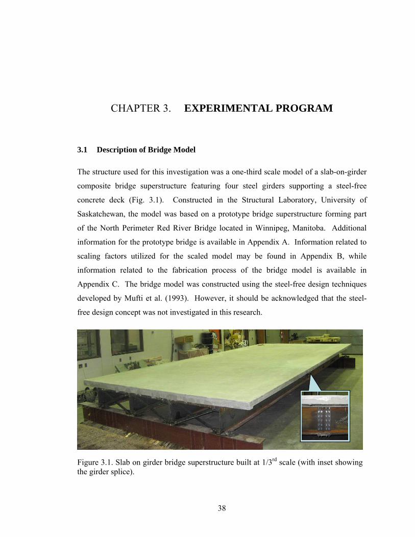
38
CHAPTER 3. EXPERIMENTAL PROGRAM
3.1 Description of Bridge Model
The structure used for this investigation was a one-third scale model of a slab-on-girder
composite bridge superstructure featuring four steel girders supporting a steel-free
concrete deck (Fig. 3.1). Constructed in the Structural Laboratory, University of
Saskatchewan, the model was based on a prototype bridge superstructure forming part
of the North Perimeter Red River Bridge located in Winnipeg, Manitoba. Additional
information for the prototype bridge is available in Appendix A. Information related to
scaling factors utilized for the scaled model may be found in Appendix B, while
information related to the fabrication process of the bridge model is available in
Appendix C. The bridge model was constructed using the steel-free design techniques
developed by Mufti et al. (1993). However, it should be acknowledged that the steel-
free design concept was not investigated in this research.
Figure 3.1. Slab on girder bridge superstructure built at 1/3rd scale (with inset showingthe girder splice).
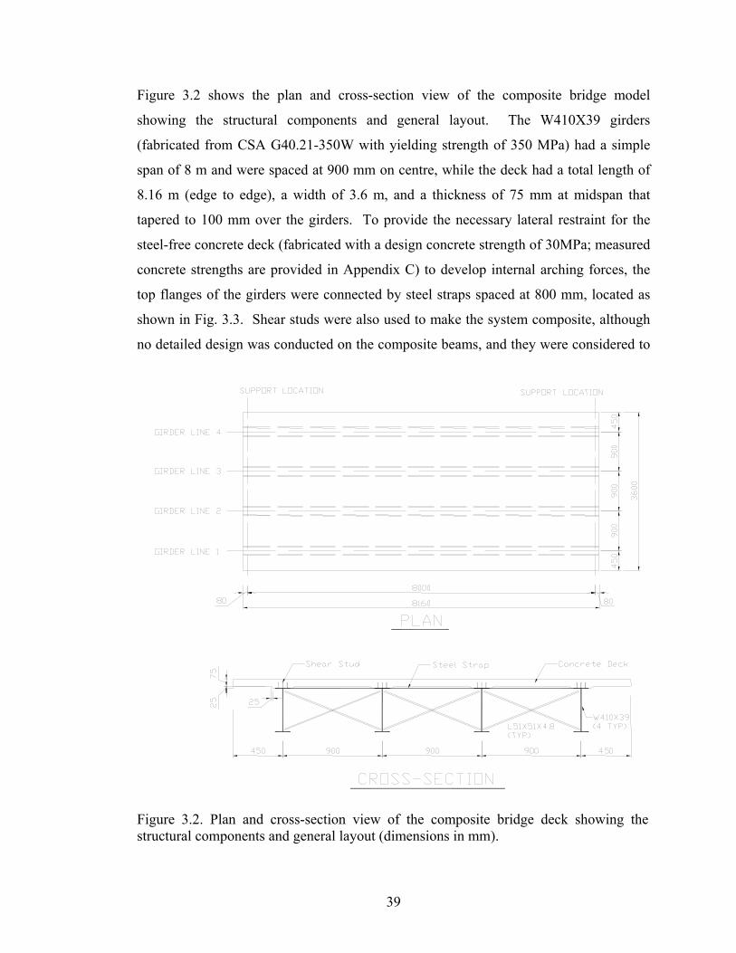
39
Figure 3.2 shows the plan and cross-section view of the composite bridge model
showing the structural components and general layout. The W410X39 girders
(fabricated from CSA G40.21-350W with yielding strength of 350 MPa) had a simple
span of 8 m and were spaced at 900 mm on centre, while the deck had a total length of
8.16 m (edge to edge), a width of 3.6 m, and a thickness of 75 mm at midspan that
tapered to 100 mm over the girders. To provide the necessary lateral restraint for the
steel-free concrete deck (fabricated with a design concrete strength of 30MPa; measured
concrete strengths are provided in Appendix C) to develop internal arching forces, the
top flanges of the girders were connected by steel straps spaced at 800 mm, located as
shown in Fig. 3.3. Shear studs were also used to make the system composite, although
no detailed design was conducted on the composite beams, and they were considered to
Figure 3.2. Plan and cross-section view of the composite bridge deck showing thestructural components and general layout (dimensions in mm).
40
be partially rather than fully composite. Diaphragms composed of cross-braced
structural angles were placed at 12 locations to enhance load sharing between girders
and provide lateral stability (denoted as D-Xx.xYy.y on Fig. 3.3, where x.x and y.y refer
to their longitudinal and transverse locations, in meters, relative to the origin shown).
To facilitate the subsequent introduction of well-defined and controlled damage states, a
number of bolted member splices and end connections were incorporated into the
model. First, a splice joint was introduced at the mid-span of Girder 4 (see the inset in
Fig. 3.1) at the location shown in Fig. 3.3 (denoted as SP-X4.0Y2.7). Splice joints were
also included at five locations on the steel straps (denoted as ST-Xx.xYy.y on Fig. 3.3,
where x.x and y.y refer to their longitudinal and transverse locations, in meters, relative
to the origin shown). Finally, all diaphragm angle members featured bolted end
connections so that any one or combination of these members could be easily
disconnected.
3.2 Measurement of Dynamic Properties
3.2.1 Overview
The basic principle of VBDD methods is that changes in dynamic properties over time
allow one to infer the nature of damage in a structure. However, the changes tend to be
Figure 3.3. Plan view of the structural steel superstructure of the model showingsplice, steel strap, and diaphragm locations (dimension in mm).
41
relatively small when the damage is minor. Furthermore, the inherent uncertainties
associated with the testing system reduce the repeatability of measured modal
properties. As a result, reliable estimates of these dynamic properties are essential for a
successful implementation of VBDD schemes.
Measurement of the modal properties of the multi-girder bridge superstructure was
carried out in two phases (see Table 3.1). In Phase I, the influence of various test
parameters on the repeatability and reliability of modal property extraction was
investigated using the intact bridge model (i.e., Health State 1, see Section 3.4). More
specifically, the test parameters that were considered in the intact bridge model tests
included sampling rates, the length of the recording period, excitation methods, sensor
type, and sensor locations (i.e., the vertical locations of strain gauges on the steel web).
Four different sampling rates were used in this investigation: 200, 500, 800, and 1000
Hz (or samples per second). To study the benefits of averaging on the reliability of the
extracted modal parameters, data recording periods of 10, 20, 40, 80, and 160 seconds
were considered. Two different forms of excitation, provided by a hydraulic shaker,
were employed: harmonic and random (white noise) forcing. For the tests conducted in
this phase, only seven accelerometer and 15 strain gauges locations (5 sets of 3 gauges
each) along Girder Line 1 were monitored to measure vertical vibration. A detailed
discussion of the results of this study is presented in Chapter 4.
In Phase II of the measurement, extensive dynamic tests were conducted on 17 Health
States (see Section 3.4) of the bridge superstructure when various specific test protocols
(see Section 3.5) were followed. The purposes of the tests were to define the damage
detection resolution of 28 different test protocols and to investigate the application of
VBDD techniques on the multi-girder bridge superstructure under various health
conditions. For the tests conducted in this phase, 28 accelerometer locations and 57
strain gauges (19 sets of 3 gauges each) over the four girder lines were used to record
the vibration signals (see Section 3.2.2). Analyses of measurement results collected in
this phase were carried out in two stages. Initially, the data were used to establish the
resolution of each test protocol, defined as the threshold value of the damage indicator
above which a change could be considered statistically significant, given the level of

42
Table 3.1. The summary of the test program.
Phase Description
Purpose:
To investigate the influence of various test parameters on the measurement reliability of the dynamic properties.
Pha
se I
Test parameters investigated: Sampling rate; Length of the recording period; Excitation method; Sensor type; Vertical location of strain gauge on the steel web.
Instrumentation and measurement points used: Seven accelerometer locations using one setup along Girder line 1; 15 strain gauges (5 sets of 3 gauges each) installed on Girder 1.
Excitation: A set of preliminary vibration tests was excited by a hydraulic frame
shaker;
Both white noise random and harmonic excitation were applied by another hydraulic shaker.
Health condition investigated: Only the intact bridge model (Health State 1, see Section 3.4).
Pha
se I
I
Purpose: To define the damage detection resolutions of different test protocols; To investigate the application of VBDD techniques on the multi-girder
bridge superstructure.
Test protocols investigated (28 in total, see Section 3.5):
Four instrumentation schemes;
Two forced excitation methods; and
Five different modes.
Instrumentation and measurement points used:
28 accelerometer locations using 5 setups
57 strain gauges (19 sets of 3 gauges each)
Excitation:
Both white noise random and harmonic excitation were applied by the hydraulic shaker.
Health condition investigated:
17 Health States (see Section 3.4).
43
uncertainty associated with that protocol. Subsequently, the performance of selected
VBDD indicators was investigated on the bridge superstructure under the 17 Health
States. A detailed discussion of the results for this phase is presented in Chapter 6.
3.2.2 Instrumentation
3.2.2.1 Overview
Instrumentation used to measure the dynamic response included a closely-spaced grid of
accelerometers mounted on the surface of the deck along the girder lines, as well as
electrical-resistance foil strain gauges bonded to the girder webs.
3.2.2.2 Accelerometers
In this study, seven accelerometers (EpiSensor FBA ES-U, manufactured by
Kinemetrics Inc., California, USA) were used. With a maximum measurement range of
0-4 g and response bandwidth from DC to 200 Hz, the low-noise force-balance uniaxial
accelerometers are ideal for civil engineering applications, where the structural response
is generally of small magnitude and whose natural frequencies are usually below 50 Hz
(Ward 1984, Levi 1997). For the vibration tests of this research, the accelerometers
were configured for a maximum range of ±0.5g with a precision of 0.00025g. A typical
accelerometer is shown in Fig. 3.4.
Different accelerometers may exhibit different levels of vibration response for a given
input excitation. As a result, a set of preliminary tests was carried out to quantify the
differences between the seven accelerometers and to find their corresponding calibration
factors relative to each other. This was done by stacking the seven accelerometers one
on top of the other into a channel-like device, and then attaching the device onto the
bridge deck (see Fig. 3.5 for the setup).
To have efficient calibration measurements, the bridge system and the attached
accelerometers were excited by the hydraulic shaker using harmonic loads with different
frequencies. For example, the input frequencies of 12.70 and 34.56 Hz (the 1st and 3rd
natural frequencies of the system, respectively, see Section 4.2.2 for the natural

44
Figure 3.5. Calibration of the EpiSensor FBA ES-U accelerometers for mode shapemeasurement.
Figure 3.4. EpiSensor FBA ES-U accelerometer.

45
frequencies of the system) were selected to excite the bridge to produce a resonant
response. The measured mode shape amplitudes and resulting calibration factors for
Mode 1 and Mode 3 are listed in Table 3.2, in which the values were averaged from
results of 20 trials after the mode shape amplitudes were normalized to the reference
channel (or Ch 2).
From the results shown in Table 3.2, it can seen that the mode shape amplitudes varied
from 0.9955 to 1.0046 for Mode 1, and from 0.9998 to 1.0127 for Mode 3. Thus, the
maximum relative differences in mode shape amplitude measurement between the seven
channels were 0.93% and 1.27% for Mode 1 and Mode 3, respectively; these relatively
small differences suggest that measurements from each accelerometer were close to
identical.
To improve the repeatability of mode shape measurements, it may be useful to apply the
corresponding calibration factors shown in Table 3.2 to the measurements of each
channel. However, the calibration factors are different for different mode shapes, as
shown in Table 3.2. For example, the calibration factors of Channel 7 were 1.0018 for
Mode 1 and 0.9875 for Mode 3, which means that the readings of this channel need to
be increased by 1.0018 for Mode 1, while needing to be decreased by 0.9875 for Mode
3. As result, not only the values, but also the trends for the calibration are different for
different modes.
Table 3.2. The summary of accelerometer calibration factors from 20 trials.
Mode 1 Mode 3 Channels Averaged mode Calibration factor Averaged mode Calibration factor
Ch 1 0.9955 1.0046 1.0017 0.9983 Ch 2* 1.0000 1.0000 1.0000 1.0000 Ch 3 1.0048 0.9952 1.0028 0.9972 Ch 4 1.0020 0.9980 1.0034 0.9967 Ch 5 0.9976 1.0024 0.9998 1.0002 Ch 6 0.9984 1.0016 1.0034 0.9967 Ch 7 0.9982 1.0018 1.0127 0.9875
*: Reference channel.
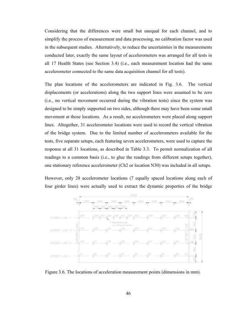
46
Considering that the differences were small but unequal for each channel, and to
simplify the process of measurement and data processing, no calibration factor was used
in the subsequent studies. Alternatively, to reduce the uncertainties in the measurements
conducted later, exactly the same layout of accelerometers was arranged for all tests in
all 17 Health States (see Section 3.4) (i.e., each measurement location had the same
accelerometer connected to the same data acquisition channel for all tests).
The plan locations of the accelerometers are indicated in Fig. 3.6. The vertical
displacements (or accelerations) along the two support lines were assumed to be zero
(i.e., no vertical movement occurred during the vibration tests) since the system was
designed to be simply supported on two sides, although there may have been some small
movement at those locations. As a result, no accelerometers were placed along support
lines. Altogether, 31 accelerometer locations were used to record the vertical vibration
of the bridge system. Due to the limited number of accelerometers available for the
tests, five separate setups, each featuring seven accelerometers, were used to capture the
response at all 31 locations, as described in Table 3.3. To permit normalization of all
readings to a common basis (i.e., to glue the readings from different setups together),
one stationary reference accelerometer (Ch2 or location N30) was included in all setups.
However, only 28 accelerometer locations (7 equally spaced locations along each of
four girder lines) were actually used to extract the dynamic properties of the bridge
Figure 3.6. The locations of acceleration measurement points (dimensions in mm).
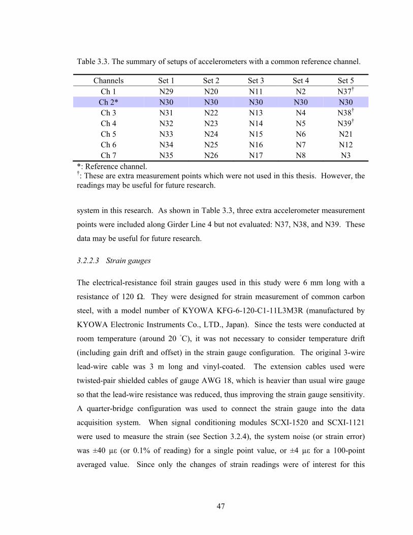
47
system in this research. As shown in Table 3.3, three extra accelerometer measurement
points were included along Girder Line 4 but not evaluated: N37, N38, and N39. These
data may be useful for future research.
3.2.2.3 Strain gauges
The electrical-resistance foil strain gauges used in this study were 6 mm long with a
resistance of 120 Ω. They were designed for strain measurement of common carbon
steel, with a model number of KYOWA KFG-6-120-C1-11L3M3R (manufactured by
KYOWA Electronic Instruments Co., LTD., Japan). Since the tests were conducted at
room temperature (around 20 C), it was not necessary to consider temperature drift
(including gain drift and offset) in the strain gauge configuration. The original 3-wire
lead-wire cable was 3 m long and vinyl-coated. The extension cables used were
twisted-pair shielded cables of gauge AWG 18, which is heavier than usual wire gauge
so that the lead-wire resistance was reduced, thus improving the strain gauge sensitivity.
A quarter-bridge configuration was used to connect the strain gauge into the data
acquisition system. When signal conditioning modules SCXI-1520 and SCXI-1121
were used to measure the strain (see Section 3.2.4), the system noise (or strain error)
was ±40 µε (or 0.1% of reading) for a single point value, or ±4 µε for a 100-point
averaged value. Since only the changes of strain readings were of interest for this
Table 3.3. The summary of setups of accelerometers with a common reference channel.
Channels Set 1 Set 2 Set 3 Set 4 Set 5 Ch 1 N29 N20 N11 N2 N37† Ch 2* N30 N30 N30 N30 N30 Ch 3 N31 N22 N13 N4 N38† Ch 4 N32 N23 N14 N5 N39† Ch 5 N33 N24 N15 N6 N21 Ch 6 N34 N25 N16 N7 N12 Ch 7 N35 N26 N17 N8 N3
*: Reference channel. †: These are extra measurement points which were not used in this thesis. However, the readings may be useful for future research.

48
research, the small initial offset and drift of the strain readings were compensated for
during the digital data processing (see Section 3.3).
In total, 57 strain gauges (19 sets of 3 gauges each) were bonded to the girder webs in
vertically aligned sets of three gauges to facilitate the determination of girder curvatures.
The plan locations of the groups of strain gauges are indicated in Fig. 3.7. There were
no strain gauges installed at the mid-span of Girder 4 due to the fact that a splice was
present at that location. Figure 3.8 shows a typical installation. In subsequent
discussions, the three strain gauges at each instrumented girder web location are
designated as the bottom, middle, and top strain gauges, which were located,
respectively, at 65, 170, and 275 mm above the bottom of the bottom flange of the
girders. This corresponds to distances of 313, 208, and 103 mm, respectively, below the
estimated neutral axis, where the averaged neutral axis location was calculated from the
strain gauge sets at all 19 locations, and extracted from dynamic test data. Figure 3.9
shows the typical setup of the strain gauges on the girder web (see Section 3.2.4 for data
acquisition and Section 3.3 for data processing of strain data in detail).
Figure 3.7. Plan view of bridge deck, showing the locations of strain gauge clusters(dimensions in mm).

49
Figure 3.9. Setup of the strain gauge sets on the girder web (19 typical, dimensionsin mm).
Steel girder
Initial plane
Estimated neutral axis
Top strain gauge
Middle strain gauge
Bottom strain gauge
Assumed deformed planeConcrete deck
105
105
65
100
399
Figure 3.8. KYOWA KFG-6-120-C1-11L3M3R electronic strain gauges bonded on thegirder web of the bridge deck.

50
3.2.3 Excitation force
To accurately measure the dynamic properties of a bridge, the structure has to be excited
to a certain level (depending on the sensitivity of sensors used). Although readily
accessible for field vibration tests, traffic and other ambient loads, which are random in
nature and difficult to quantify, introduce considerable uncertainty into the extracted
modal properties of a bridge. Ambient environmental excitations in a laboratory have
also proven to be unreliable sources for dynamic tests. Controlled excitations, on the
other hand, appear to be more reliable for the extraction of modal properties, especially
for VBDD applications (Wegner et al. 2004). As a result, controlled excitation forces
were used in this research to excite the bridge model for dynamic tests.
Initially, a set of preliminary test was performed. For the preliminary tests, a hydraulic
frame-mounted shaker was applied on the surface of the concrete deck to excite the
bridge (see Fig. 3.10). The shaker consisted of a hydraulic cylinder mounted vertically
on the frame, which was bolted down to the laboratory strong floor. The shaker was
capable of exciting the bridge model to measure the dynamic properties with relatively
high level of repeatability. However, the measured mode shapes were somewhat
different from the expected results, which may have been due to the extra restraints
applied at the contact points on the deck surface from the fixed frame. To accurately
measure the modal properties of the system, the frame-mounted hydraulic shaker was
abandoned for subsequent tests.
To fit the purpose of the dynamic tests, another hydraulic shaker was built based on a
shaker available in the Mechanical Laboratory, University of Saskatchewan. The new
shaker consisted of a hydraulic cylinder mounted vertically in the centre of a steel
frame, with a steel plate of a selected mass (75 lb or 34.02 kg) supported at the bottom
end of the cylinder (Fig. 3.11). The shaker was securely attached to the surface of the
bridge deck using a bracket that was bolted to threaded inserts embedded in the concrete
deck. The location of the shaker, along Girder Line 2 at a distance of 2.5 m from the
left support, was chosen to permit excitation of the vibration modes of interest (the
lowest five modes) after several preliminary tests were conducted at other locations.

51
Excitation forces applied in the experimental tests included both harmonic and white
noise random vibration loads applied by the hydraulic shaker.
A hardware feedback-controlled signal for the shaker plate motion was generated using
LabViewTM 8.0 software installed on a laptop computer and monitored using a linear
displacement transducer (LDT). The input signal for the shaker plate was controlled by
a separate data acquisition system (or, more specifically for this application, a system
controller), and consisting of a data acquisition PCMCIA card (model NI DAQ Card-
6036E), SCXI-1000 data acquisition chassis, and several other modules from National
InstrumentsTM. This system was independent of the data acquisition system used for
recording the accelerometer, strain gauge, and LDT readings (see details in Section
3.2.4). The reason for using two separate data acquisition systems (or, rather, a system
controller and a data acquisition system) was that when only one system was used, the
software feedback controller failed to control the shaker effectively and record the data
simultaneously. As a result, a hardware feedback controller was developed to control
Figure 3.10. The hydraulic frame-mounted shaker used for preliminary tests.

52
the fluid flow in a proportional directional valve, with a model number of KBSDG4V-5,
(manufactured by Vickers, Incorporated, USA); the user’s manual for the developed
hardware controller is available in Appendix L. Thus, two separate data acquisition
systems, one for input and another for output, were adopted in the tests.
To identify the natural frequencies of the system for each condition tested, white noise
random signals were initially used to excite the bridge deck. In fact, the corresponding
mode shapes were also extracted in this manner, but with relatively lower accuracy than
the procedure described below. White noise random forces, a special random process,
were adopted to excite the bridge partially due to their characteristic feature of having
an approximately constant amplitude for all frequencies in the power spectrum density
function. Based on random vibration theory, the displacement response power spectrum
of a linear system is defined as the product of the power spectrum density function of
the input and the frequency response function. Since the power spectrum density
function of a white noise random signal is theoretically constant, the shape of the
Figure 3.11. The hydraulic shaker used to excite both resonant harmonic and white noisenoise random vibration in the experiments.

53
displacement or acceleration response spectrum is the same as that of the system’s
frequency response function, with only the amplitude being different. In this manner,
the natural frequencies of the system can be identified with a high degree of accuracy
through measuring the displacement (or acceleration) response spectrum, with less
influence of the excitation forces on the measured modal properties. This is especially
important for the output-only identification method adopted in this research, for which it
was assumed that the input forces were unknown, even though the input signals were
recorded through the LDT readings. The LDT readings may be useful for future
research.
After the natural frequencies had been identified, further testing using harmonic (or
purely sinusoidal) excitation applied at each individual natural frequency was
undertaken to accurately measure the corresponding mode shapes. Higher measurement
accuracy was possible using this method because a resonant response, with a large
constant amplitude vibration, occurred when the frequency of the harmonic excitation
force coincided with one of the natural frequencies of the system.
3.2.4 Data acquisition
Data were acquired using a data acquisition system consisting of a 12-bit NI PCI-6024E
data acquisition card and a model SCXI-1001 data acquisition chassis from National
InstrumentsTM, along with 12 signal conditioning modules (one SCXI-1120, four SCXI-
1520, and seven SCXI-1121) used to acquire and modulate the sensor signals from both
accelerometers and strain gauges (see Fig. 3.12 for the setup of the data acquisition
system).
The 12-bit resolution means that the range of the measured signal could be divided into
212 segments, for a resolution of 1 in 4096. The data acquisition card had built-in 16
channels (in a single-ended configuration) or 8 channels (in the differential
configuration). However, actually, no built-in internal channels of the card were used to
collect any data. The NI PCI-6024E card was only treated as an analog-to-digital
converter (ADC), which converted the analog signals from the twelve signal
conditioning modules installed in the Chassis SCXI-1001. The ADC still had 12-bit
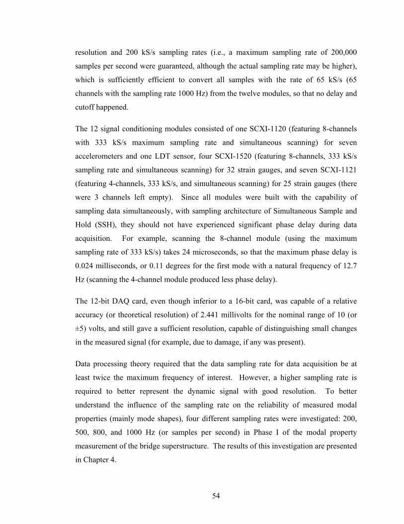
54
resolution and 200 kS/s sampling rates (i.e., a maximum sampling rate of 200,000
samples per second were guaranteed, although the actual sampling rate may be higher),
which is sufficiently efficient to convert all samples with the rate of 65 kS/s (65
channels with the sampling rate 1000 Hz) from the twelve modules, so that no delay and
cutoff happened.
The 12 signal conditioning modules consisted of one SCXI-1120 (featuring 8-channels
with 333 kS/s maximum sampling rate and simultaneous scanning) for seven
accelerometers and one LDT sensor, four SCXI-1520 (featuring 8-channels, 333 kS/s
sampling rate and simultaneous scanning) for 32 strain gauges, and seven SCXI-1121
(featuring 4-channels, 333 kS/s, and simultaneous scanning) for 25 strain gauges (there
were 3 channels left empty). Since all modules were built with the capability of
sampling data simultaneously, with sampling architecture of Simultaneous Sample and
Hold (SSH), they should not have experienced significant phase delay during data
acquisition. For example, scanning the 8-channel module (using the maximum
sampling rate of 333 kS/s) takes 24 microseconds, so that the maximum phase delay is
0.024 milliseconds, or 0.11 degrees for the first mode with a natural frequency of 12.7
Hz (scanning the 4-channel module produced less phase delay).
The 12-bit DAQ card, even though inferior to a 16-bit card, was capable of a relative
accuracy (or theoretical resolution) of 2.441 millivolts for the nominal range of 10 (or
±5) volts, and still gave a sufficient resolution, capable of distinguishing small changes
in the measured signal (for example, due to damage, if any was present).
Data processing theory required that the data sampling rate for data acquisition be at
least twice the maximum frequency of interest. However, a higher sampling rate is
required to better represent the dynamic signal with good resolution. To better
understand the influence of the sampling rate on the reliability of measured modal
properties (mainly mode shapes), four different sampling rates were investigated: 200,
500, 800, and 1000 Hz (or samples per second) in Phase I of the modal property
measurement of the bridge superstructure. The results of this investigation are presented
in Chapter 4.
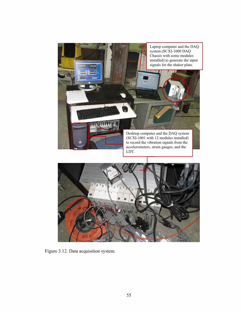
55
Laptop computer and the DAQ system (SCXI-1000 DAQ Chassis with some modules installed) to generate the input signals for the shaker plate.
Desktop computer and the DAQ system (SCXI-1001 with 12 modules installed) to record the vibration signals from the accelerometers, strain gauges, and the LDT.
Figure 3.12. Data acquisition system.
56
The data acquisition system was controlled by LabViewTM software installed on a
personal computer. To identify the natural frequencies of the system for each condition
tested, white noise random signals were initially used to excite the bridge deck, while
data were acquired at 1000 samples per second. In this manner, the natural frequencies
for the first five vibration modes of the undamaged model were found to be 12.70,
13.89, 34.56, 35.89, and 38.83 Hz. After the natural frequencies had been identified,
further testing using harmonic excitation applied at each individual natural frequency
was undertaken to accurately measure the corresponding mode shapes. For these tests,
data were acquired at 500 samples per second. The lower sampling rate was used due to
the lower uncertainty associated with harmonic excitation compared with white noise
random excitation. A detailed explanation is available in Chapter 4.
For each health state investigated (as described in Section 3.4), the data for all 65
channels were continuously recorded in one file and instantaneously saved on the hard
drive of the personal computer. A sampling period of 800 seconds of data was saved for
each white noise excitation input, while 400 seconds of data were saved for each
harmonic excitation input. In this manner, for each health state, five files were
generated when white noise excitation was used, one file for each of the five separate
setups for the accelerometers, as described in Section 3.2. Each file contained data for
all vibration modes and was 580 Mega-bytes in size. Ten files were generated for each
health state when harmonic excitation was used, five for the first mode (one per
accelerometer setup), and five for the second mode. Each of these files was 145 Mega-
bytes in size.
3.3 Data Processing
Data processing consisted of two steps, referred to here as data pre-processing and post-
processing. Figure 3.13 shows a flow chart for data processing. Data were
preprocessed by applying filtering, averaging, and windowing before the post
processing to obtain modal properties.
In the first step, the data were separated into individual files for each sensor type (i.e.,
accelerometers, strain gauges, and LDT) and each 80 s segment of data. In this manner,
57
for each health state, twenty-five files for each of the three different sensor types were
generated when harmonic excitation was used (five segments of 80 seconds for each of
five accelerometer setups), while fifty files were generated when white noise excitation
was used (ten segments of 80 seconds for each of five setups). Any combination of five
files (one from each one of the five accelerometer setups) for acceleration was able to
define one vibration mode (for harmonic excitation) or one set of multiple vibration
modes (i.e., the 1st to the 5th mode, for white noise excitation). As a result, this process
could produce 3125 (or 55) possible trials for vibration modes with harmonic excitation;
while 105 possible trials were available for vibration modes with white noise excitation
(these trials are only partially independent from each other). However, only five trials
(i.e., the combinations of T11111, T22222, T33333, T44444, and T55555, where s in Tsssss denotes
the sequence of segments), which are totally independent from each other, were
generated and used in the subsequent sections of this thesis for both harmonic (the 1st
and 2nd mode) and white noise excitations (the 1st to the 5th mode ). On the other hand,
each file for strain gauges was able to define the vibration mode (or modes) of the whole
bridge model by itself. Therefore, twenty-five trials were available for definition of
mode shapes when harmonic inputs were used, while fifty trials were available to define
the mode shapes when white noise excitation was used. It should be noted that the
process of file separation experienced some challenges due to the extremely large size
files (up to 580 Mega-bytes per file). A LabView subroutine was finally developed to
perform the separation process by dynamically reading the original files, processing, and
writing to separate files. This is similar to the way that LabView records data to files.
After the data were separated into individual files according to sensor types, a “detrend”
subroutine available in Matlab (2004) was used to remove any average baseline offset
(DC components) and linear trends from the recorded data by means of a linear
regression process. A moving average low-pass filter, decimating the data by an order
of 5, was adopted to filter the signals, resulting in a smoothed signal at a lower sampling
rate. In this way, the inherent random noise was reduced through the moving average
technique, which could increase the accuracy of the measured dynamic properties. The
resulting effective sampling rates were 100 Hz for harmonic excitation and 200 Hz for
random white noise excitation.
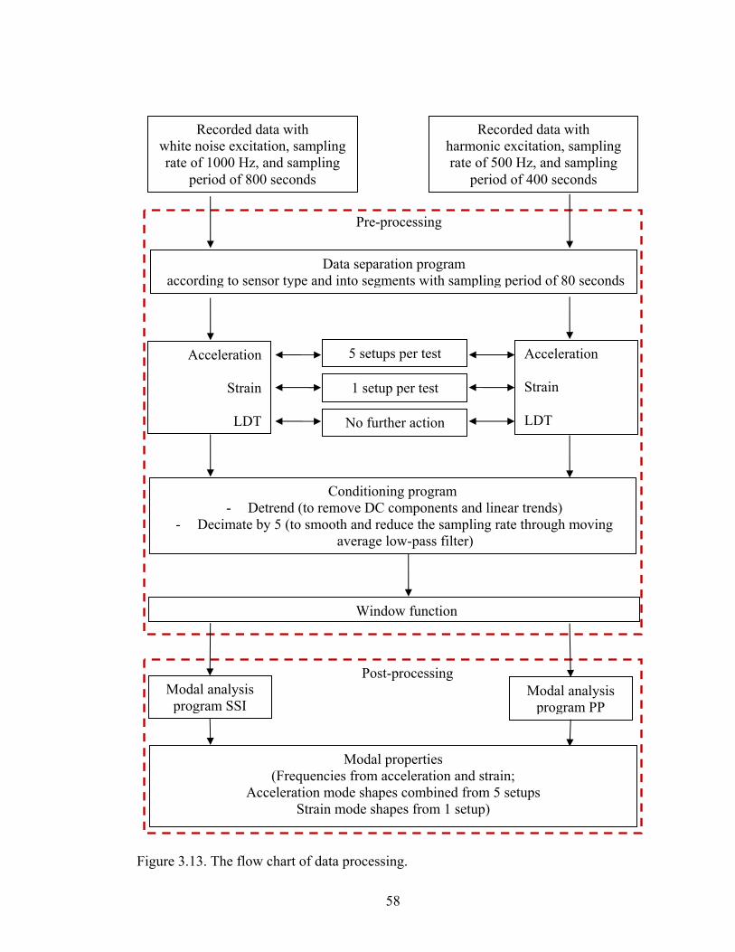
58
Post-processing
Pre-processing
Figure 3.13. The flow chart of data processing.
Recorded data with white noise excitation, sampling rate of 1000 Hz, and sampling
period of 800 seconds
Data separation program according to sensor type and into segments with sampling period of 80 seconds
Recorded data with harmonic excitation, sampling rate of 500 Hz, and sampling
period of 400 seconds
Acceleration
Strain
LDT
Acceleration Strain LDT
Conditioning program - Detrend (to remove DC components and linear trends)
- Decimate by 5 (to smooth and reduce the sampling rate through moving average low-pass filter)
Window function
Modal analysis program SSI
Modal analysis program PP
Modal properties (Frequencies from acceleration and strain;
Acceleration mode shapes combined from 5 setups Strain mode shapes from 1 setup)
No further action
1 setup per test
5 setups per test
59
A Hanning window (Mathworks 2006, Ramirez 1985) was used to reduce “leakage” in
the resulting spectrum. Leakage occurs when signals are truncated at either their
beginning or end, so that the spectral energy appears to spread to neighboring
frequencies (Maia and Silva 1997). However, it was found in the current tests that the
window function had little influence on the accuracy of measured modal properties. In
fact, there was no noticeable difference between measured modal properties no matter
which window function was used or whether or not a window function was used at all.
This may be partially due to the fact that a relatively long sampling period of 80 seconds
was used, compared with the fundamental period of 0.079 seconds (i.e., the sampling
period was 1016 times the fundamental period), and that well-controlled excitation
forces were adopted to excite the bridge model. Controlled excitation appears to
produce more periodic data than environmental or traffic excitations. As a result, no
further study was conducted on the performance of window functions, even though
window functions are usually considered to be important for processing dynamic test
data.
In the post-processing phase, the modal properties of the bridge model were extracted
from the pre-processed sensor data, using both the Pick Picking method (PP) (Section
2.4.2), and the Stochastic Subspace Identification method (SSI) (Section 2.4.3), as
implemented in the commercially available software package SPICE (or MACEC) (Van
den Branden et al. 1999, Van Overschee and De Moor 1996). For the purposes of
modal parameter estimation, it was assumed that the exciting force was not known or
measured, so that “output-only” modal extraction techniques were required. A
comparison between the PP and SSI methods is presented in Chapter 4 in terms of their
influence on the reliability of extracted modal properties. The results in Chapter 4 show
that the SSI method provided more reliable modal properties than the PP method when
white noise excitation was used. For subsequent investigations, therefore, the SSI
method was used for modal analysis of the data with white noise excitation, while the
PP method was adopted for the processing of data with harmonic excitation to take
advantage of faster processing, the more straightforward procedure, and comparable
reliability of measured modal properties.
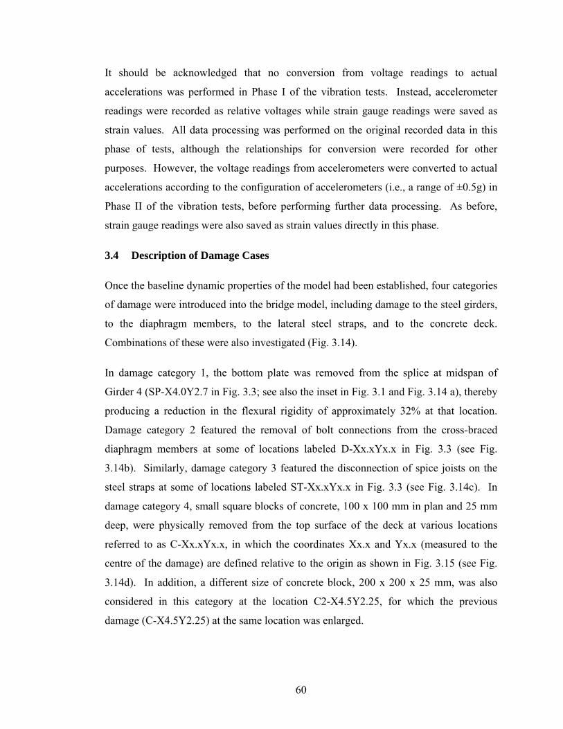
60
It should be acknowledged that no conversion from voltage readings to actual
accelerations was performed in Phase I of the vibration tests. Instead, accelerometer
readings were recorded as relative voltages while strain gauge readings were saved as
strain values. All data processing was performed on the original recorded data in this
phase of tests, although the relationships for conversion were recorded for other
purposes. However, the voltage readings from accelerometers were converted to actual
accelerations according to the configuration of accelerometers (i.e., a range of ±0.5g) in
Phase II of the vibration tests, before performing further data processing. As before,
strain gauge readings were also saved as strain values directly in this phase.
3.4 Description of Damage Cases
Once the baseline dynamic properties of the model had been established, four categories
of damage were introduced into the bridge model, including damage to the steel girders,
to the diaphragm members, to the lateral steel straps, and to the concrete deck.
Combinations of these were also investigated (Fig. 3.14).
In damage category 1, the bottom plate was removed from the splice at midspan of
Girder 4 (SP-X4.0Y2.7 in Fig. 3.3; see also the inset in Fig. 3.1 and Fig. 3.14 a), thereby
producing a reduction in the flexural rigidity of approximately 32% at that location.
Damage category 2 featured the removal of bolt connections from the cross-braced
diaphragm members at some of locations labeled D-Xx.xYx.x in Fig. 3.3 (see Fig.
3.14b). Similarly, damage category 3 featured the disconnection of spice joists on the
steel straps at some of locations labeled ST-Xx.xYx.x in Fig. 3.3 (see Fig. 3.14c). In
damage category 4, small square blocks of concrete, 100 x 100 mm in plan and 25 mm
deep, were physically removed from the top surface of the deck at various locations
referred to as C-Xx.xYx.x, in which the coordinates Xx.x and Yx.x (measured to the
centre of the damage) are defined relative to the origin as shown in Fig. 3.15 (see Fig.
3.14d). In addition, a different size of concrete block, 200 x 200 x 25 mm, was also
considered in this category at the location C2-X4.5Y2.25, for which the previous
damage (C-X4.5Y2.25) at the same location was enlarged.
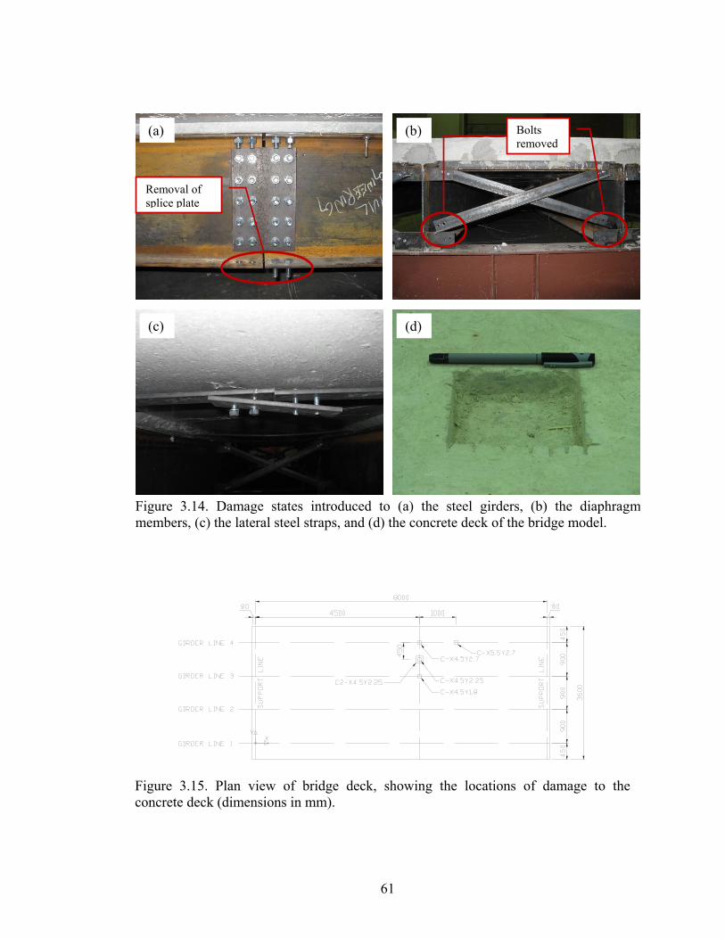
61
Figure 3.15. Plan view of bridge deck, showing the locations of damage to theconcrete deck (dimensions in mm).
Figure 3.14. Damage states introduced to (a) the steel girders, (b) the diaphragmmembers, (c) the lateral steel straps, and (d) the concrete deck of the bridge model.
(a) (b)
(c) (d)
Removal of splice plate
Bolts removed

62
Vibration tests were conducted on the bridge model in seventeen different health states
(or physical conditions), while the other test parameters, including excitation forces,
sensors, and data processing methods, remained the same. Table 3.4 lists the 17 health
states, as well as the descriptions for each health state. Health State 1 was the intact
condition, which means that no physical damage had been introduced since the bridge
model was constructed. Extensive dynamic tests were performed with the model in this
health state. Some initial tests were conducted first to establish consistent and reliable
test procedures through checking and calibrating various factors, including the
connection of cables, sensors, data acquisition system, LabView programs, suitable
excitation forces and locations, and efficient data processing procedures. Then, Phase I
tests were conducted to investigate the influence of several testing parameters on the
variability of measured modal properties, as described in Section 3.2.1. In this phase,
only the data from Girder Line 1 were used for this purpose, and results are presented in
Chapter 4.
After the testing parameters were quantified in Phase I, the vibration tests carried out in
Phase II were conducted with selected values of some testing parameters to measure
both the natural frequencies and mode shapes of the whole superstructure bridge model
over all girder lines. For example, a combination of sampling rate of 1000 Hz and
sampling period of 800 seconds was used to record the vibration data for white noise
excitation cases. The measured modal properties are evaluated in Chapter 4. The modal
properties in Health State 1 were also used as a baseline for some of the other health
states for damage detection. A detailed discussion of damage detection is available in
Chapter 6.
For Health States 2 to 5, a new state of damage was incrementally introduced in the
model without repairing previous damage. The individual damage states and
combinations of these states included damage to the steel girder splice and the cross
bracing diaphragms at different locations (SP-X4.0Y2.7, D-X5.2Y2.25, D-X8.0Y1.35,
and D-X0.0Y2.25).

63
For Health States 6 to 10, a new state of damage was introduced into the model after all
previous damage had been repaired, except for the damage to the steel girder splice (SP-
X4.0Y2.7). The new damage states considered included damage to the diaphragms and
the steel straps at various locations. The purpose of these damage states was an attempt
to investigate the influence of damage location on the performance of VBDD methods
Table 3.4. The health states investigated on the bridge model.
Health States
Description of Health States
State 1 Intact condition State 2 SP-X4.0Y2.7 State 3 SP-X4.0Y2.7 and D-X5.2Y2.25 State 4 SP-X4.0Y2.7, D-X5.2Y2.25, and D-X8.0Y1.35 State 5 SP-X4.0Y2.7, D-X5.2Y2.25, D-X8.0Y1.35, and D-X0.0Y2.25 State 6 SP-X4.0Y2.7 and D-X8.0Y1.35 State 7 SP-X4.0Y2.7 and D-X0.0Y0.45 State 8 SP-X4.0Y2.7 and D-X2.8Y1.35 State 9 SP-X4.0Y2.7 and ST-X6.8Y0.45 State 10 SP-X4.0Y2.7 and ST-X4.4Y0.45 State 11 SP-X4.0Y2.7, ST-X4.4Y0.45, and ST-X4.4Y1.35 State 12 SP-X4.0Y2.7, ST-X4.4Y0.45, ST-X4.4Y1.35, and ST-X4.4Y2.25 State 13 C-X4.5Y2.7 State 14 C-X4.5Y2.7 and C-X4.5Y1.8 State 15 C-X4.5Y2.7, C-X4.5Y1.8, and C-X5.5Y2.7 State 16 C-X4.5Y2.7, C-X4.5Y1.8, C-X5.5Y2.7, and C-X4.5Y2.25 State 17 C-X4.5Y2.7, C-X4.5Y1.8, C-X5.5Y2.7, C-X4.5Y2.25, and C2-X4.5Y2.25
X4.0Y2.7 indicates that the damage was located at x and y coordinates of 4.0 m and 2.7 m, respectively, as defined in Fig. 3.3; SP = The splice joint in Girder 4 was disconnected at location Xx.xYy.y; D = Diaphragms were disconnected at location Xx.xYy.y; ST = Splice joints on the steel straps were disconnected at location Xx.xYy.y; C = Concrete block with dimension of 100*100*25 mm was removed from the surface of the concrete deck at location Xx.xYy.y; C2 = Concrete block with dimension of 200*200*25 mm, on the base of the previous case C-X4.5Y2.25 at the same location, was removed from the surface of the concrete deck at location X4.5Y2.25.

64
while the severity of damage remained the same. Health States 11 and 12 considered
incremental damage to the steel straps.
Before inducing Health State 13, all previous damage was repaired by reconnecting the
members using bolts. It should be noted that the repairs could not restore the bridge
system to the original condition exactly, due to the fact that the repairs were conducted
after the model had been loaded multiple times, even though the differences may not
have been significant. A detailed discussion based on testing results is available in
Chapter 6.
For Health States 13 to 16, a new state of damage was introduced incrementally by
physically removing small square blocks of concrete (100 x 100 x 25 mm) from the top
surface of the deck at various locations. In Health State 17, a larger size of concrete
block, 200 x 200 x 25 mm, was removed, enlarging the previous damage at the same
location (i.e., the effective change in physical condition from Health State 16 to Health
State 17 was 200 x 200 x 25 mm minus 100 x 100 x 25 mm).
Damage states (to be distinguished from health states) were defined as the change in
physical properties between two health states (or conditions): the initial (or undamaged)
state and the new (or damaged) state. In this manner, a health state previously defined
as “damaged” could be reconsidered to be an “undamaged” state for subsequent health
states investigated later on. By comparing two health states listed in Table 3.4, and
treating the earlier state as the “undamaged state” and the later state as the “damaged
state”, 26 damage cases were generated and investigated in this research. For example,
to generate Damage Case 1, Health State 1 was considered as “undamaged” and Health
State 2 was considered as “damaged”. Table 3.5 lists all 26 damage cases considered,
defining the corresponding “undamaged” and “damaged” states, and describing the
damage for each damage case. The results for the application of VBDD methods to the
damage cases are discussed in Chapter 6.

65
3.5 Test Protocols Investigated
For each health state considered, 28 different test protocols were investigated, as listed
in Table 3.6, which included combinations of four different instrumentation schemes
(use of accelerometer data, use of data from only the bottom strain gauge in each cluster,
use of data from only the middle strain gauge in each cluster, and use of data from only
the top strain gauge in each cluster), two different forced excitation methods (resonant
harmonic and random white noise), and five different modes. It should be
acknowledged that the modes are not really a “test protocol”. They were simply a result
of post-processing. However, the use of different modes was actually treated as a
component of a test protocol, since there were different uncertainties involved in the
measurement of different vibration modes (see Chapter 4 and 6 for details). The lowest
five vibration modes were extracted when using random excitation, while only the
lowest two modes were investigated when using harmonic excitation. The resulting
detailed mode shape definitions and comparisons are available in Chapter 4. The
resolutions of different test protocols and the results for application of VBDD methods
under specific test protocols are presented in Chapter 6.
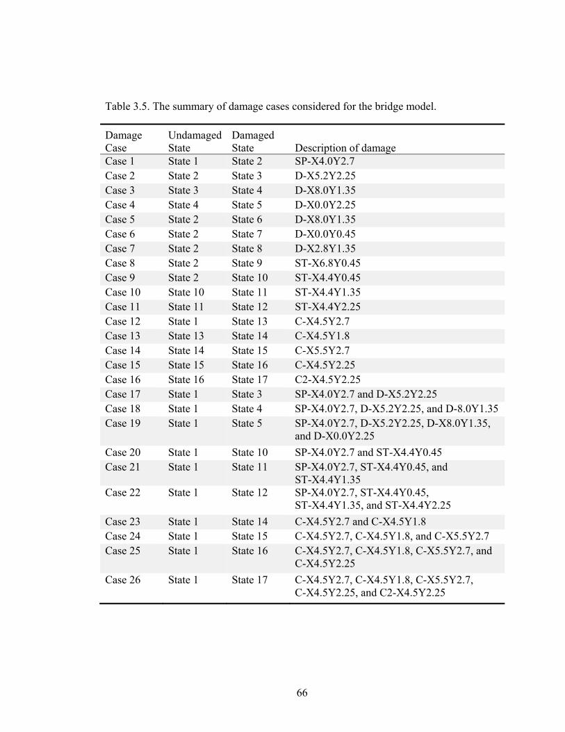
66
Table 3.5. The summary of damage cases considered for the bridge model.
Damage Case
Undamaged State
Damaged State Description of damage
Case 1 State 1 State 2 SP-X4.0Y2.7 Case 2 State 2 State 3 D-X5.2Y2.25 Case 3 State 3 State 4 D-X8.0Y1.35 Case 4 State 4 State 5 D-X0.0Y2.25 Case 5 State 2 State 6 D-X8.0Y1.35 Case 6 State 2 State 7 D-X0.0Y0.45 Case 7 State 2 State 8 D-X2.8Y1.35 Case 8 State 2 State 9 ST-X6.8Y0.45 Case 9 State 2 State 10 ST-X4.4Y0.45 Case 10 State 10 State 11 ST-X4.4Y1.35 Case 11 State 11 State 12 ST-X4.4Y2.25 Case 12 State 1 State 13 C-X4.5Y2.7 Case 13 State 13 State 14 C-X4.5Y1.8 Case 14 State 14 State 15 C-X5.5Y2.7 Case 15 State 15 State 16 C-X4.5Y2.25 Case 16 State 16 State 17 C2-X4.5Y2.25 Case 17 State 1 State 3 SP-X4.0Y2.7 and D-X5.2Y2.25 Case 18 State 1 State 4 SP-X4.0Y2.7, D-X5.2Y2.25, and D-8.0Y1.35 Case 19 State 1 State 5 SP-X4.0Y2.7, D-X5.2Y2.25, D-X8.0Y1.35,
and D-X0.0Y2.25
Case 20 State 1 State 10 SP-X4.0Y2.7 and ST-X4.4Y0.45 Case 21 State 1 State 11 SP-X4.0Y2.7, ST-X4.4Y0.45, and
ST-X4.4Y1.35 Case 22 State 1 State 12 SP-X4.0Y2.7, ST-X4.4Y0.45,
ST-X4.4Y1.35, and ST-X4.4Y2.25
Case 23 State 1 State 14 C-X4.5Y2.7 and C-X4.5Y1.8 Case 24 State 1 State 15 C-X4.5Y2.7, C-X4.5Y1.8, and C-X5.5Y2.7 Case 25 State 1 State 16 C-X4.5Y2.7, C-X4.5Y1.8, C-X5.5Y2.7, and
C-X4.5Y2.25
Case 26 State 1 State 17 C-X4.5Y2.7, C-X4.5Y1.8, C-X5.5Y2.7, C-X4.5Y2.25, and C2-X4.5Y2.25

67
Table 3.6. The summary of test protocols investigated.
Test Protocol Vibration Mode Excitation Instrumentation 1 Mode 1 Harmonic Accelerometer 2 Mode 1 Harmonic Bottom strain gauge 3 Mode 1 Harmonic Middle strain gauge 4 Mode 1 Harmonic Top strain gauge 5 Mode 1 White noise random Accelerometer 6 Mode 1 White noise random Bottom strain gauge 7 Mode 1 White noise random Middle strain gauge 8 Mode 1 White noise random Top strain gauge 9 Mode 2 Harmonic Accelerometer 10 Mode 2 Harmonic Bottom strain gauge 11 Mode 2 Harmonic Middle strain gauge 12 Mode 2 Harmonic Top strain gauge 13 Mode 2 White noise random Accelerometer 14 Mode 2 White noise random Bottom strain gauge 15 Mode 2 White noise random Middle strain gauge 16 Mode 2 White noise random Top strain gauge 17 Mode 3 White noise random Accelerometer 18 Mode 3 White noise random Bottom strain gauge 19 Mode 3 White noise random Middle strain gauge 20 Mode 3 White noise random Top strain gauge 21 Mode 4 White noise random Accelerometer 22 Mode 4 White noise random Bottom strain gauge 23 Mode 4 White noise random Middle strain gauge 24 Mode 4 White noise random Top strain gauge 25 Mode 5 White noise random Accelerometer 26 Mode 5 White noise random Bottom strain gauge 27 Mode 5 White noise random Middle strain gauge 28 Mode 5 White noise random Top strain gauge
68
CHAPTER 4. EXPERIMENTAL RESULTS
4.1 Overview
As explained in Chapter 3, the vibration tests were conducted in two phases, with Phase
I undertaken to investigate the influence of various testing parameters on the
repeatability and reliability of modal property extraction, and Phase II focussing on
damage detection and the sensitivity of various approaches to damage. To give a
general idea of the testing results for better understanding the whole process of testing,
some of the results for the Phase II tests are presented in this chapter first. The results of
the Phase II vibration tests presented here include the recorded vibration time history
data, the filtered time history series accompanied by the corresponding spectra, the
extracted natural frequencies using both accelerometers and strain gauges in various
health states, the lowest five mode shapes defined using both accelerometer and strain
gauge data, and a general comparison of mode shapes in various health states.
Following this, the results of the Phase I tests are presented. In particular, the influence
of sensor type and location, data sampling rate, data sampling period, and excitation
method on the repeatability and reliability of modal property extraction are presented.
Since the amplitude of mode shapes is indeterminate in most cases, it is necessary to
normalize (or scale) the mode shapes to a common base in order to identify the changes
in mode shapes caused by damage. An investigation of the influence of normalization
methods and schemes on the definition of mode shapes and changes in mode shapes was
conducted, with results presented in this chapter. To clarify, the term “normalization
method” is used to refer to the method used to scale the mode shape, while
“normalization scheme” refers to whether the entire structure is considered as a unit
during the normalization process, or different subsets of the structure are normalized

69
separately. A new normalization method was developed as part of this work.
Comparisons among various normalization methods and two different schemes were
preformed. The results of the comparison are presented in this chapter.
4.2 Dynamic Properties of the Bridge Model
4.2.1 Recorded vibration data and the corresponding modal identification
Figure 4.1 (a) shows a typical acceleration time history of the original recorded data
Figure 4.1. Vibration response to random white noise excitation for the originalrecorded reference accelerometer data: (a) acceleration time history; (b) accelerationspectrum.
(a)
(b)
70
induced by the random white noise excitation, while Figure 4.1 (b) presents the
corresponding acceleration frequency spectrum of the same signal. The signal shown in
Fig. 4.1 was recorded by the reference accelerometer (see Table 3.3) for the Health State
1 (i.e., the intact condition). The signals for other channels in other health states were
similar to those shown in Fig. 4.1, except that they exhibited different amplitudes and
small shifts in frequencies. From Fig. 4.1 (b), it can be seen that the maximum
frequency (usually called the Nyquist frequency) in the frequency spectrum plot is 500
Hz, which is one-half of the sampling rate of 1000 Hz, based on Nyquist–Shannon
sampling theorem (Marks 1991). This sampling theorem supplied a sufficient condition,
under which bandlimited signals (i.e., signals which have a maximum frequency) can be
reconstructed perfectly from their sampled data, if the sampling rate is more than twice
the maximum frequency. As a result, the frequency equal to one-half of the sampling
rate is the highest frequency that can be unambiguously represented by the sampled
signal. The relatively high sampling rate was adopted to take advantage of the benefit
of oversampling and then, using low-pass digital filter techniques, to allow for the
decimation of the digitized data. In this manner, the inherent random noise could be
reduced, potentially increasing the accuracy of measured dynamic properties.
The frequencies of interest for civil engineering structures are usually below 50 Hz.
Specifically, in this case, the signals were decimated to a lower sampling rate of 200 Hz,
which resulted in a maximum frequency of 100 Hz in the frequency spectrum. Figure
4.2 (a) shows the decimated results for the same signal, while Fig. 4.2 (b) presents the
corresponding spectrum of the decimated signal from the 80 second record (16000
sampling points), in which the maximum frequency is 100 Hz. Figure 4.2 (c) presents
the averaged spectrum from ten equal length segments of the record, which did not
feature any overlap but were modified by a Hanning window (see Section 3.3). To
clarify, the 80 second record was divided into ten segments of equal length, with 1600
sampling points each. As a result, the spectrum shown in Fig. 4.2 (c) features much less
noise. To more clearly show the decimated signal and the corresponding frequency
spectrum, Fig. 4.3 presents a two second segment of the signal and frequency spectra up
to 45 Hz (a closer view of Fig. 4.2).

71
Figure 4.2. Vibration response to random white noise excitation for the decimatedaccelerometer data: (a) acceleration time history; (b) spectrum from one record; (c)averaged spectrum from ten equal length segments without overlap using a Hanningwindow.
(a)
(b)
(c)

72
Figure 4.3. Closer view of vibration response to random white noise excitation for thedecimated accelerometer data: (a) acceleration time history (a two second segment ofthe signal); (b) spectrum from one record (up to 45 Hz); (c) averaged spectrum from tenequal length segments without overlap using a Hanning window (up to 45 Hz).
(a)
(b)
(c)

73
In the same manner, Fig. 4.4 presents a closer view of a typical strain response to
random white noise excitation, in this case for a bottom strain gauge. The signal shown
in Fig. 4.4 (a) came from a bottom strain gauge channel located at the mid-span of
Girder 1 during the same test that produced the signal shown in Fig. 4.3 (a). The
amplitude of the frequency spectrum in the region of 35 Hz was much smaller in Fig.
4.4 (b) and (c) than that present in Fig. 4.3 (b) and (c), which may due to the fact that the
strain gauges used in the tests are generally not as sensitive to higher frequency
vibration as the accelerometers that were used. This means that the accelerometers may
generate more accurate higher frequency data than the strain gauges.
The many peaks observed in both Fig. 4.3 (b) and Fig. 4.4 (b) demonstrate that it was
difficult to reliably identify the natural frequencies of the system using the PP method,
especially in the vicinity of 35 Hz. As a result, the SSI method, a time domain modal
analysis method, as implemented in the commercially available software SPICE (or
MACEC) (Van den Branden et al. 1999, Van Overschee and De Moor 1996) was
adopted to identify the natural frequencies and the corresponding mode shapes of the
system. Figure 4.5 shows the stabilization plots (implemented in the software SPICE)
to identify the modal properties of the bridge superstructure, where Fig. 4.5 (a)
corresponds to the accelerometer signal shown in Fig. 4.3 (a) and Fig. 4.5 (b)
corresponds to the bottom strain gauge signal shown in Fig. 4.4 (a). Stabilization plots
show the stability of the poles (using symbols of “+” in the plots) as a function of
increasing model order (plotted in the vertical axis, and denoting the order of the sub-
space) under certain pre-set stabilization criteria (here this was set at 0.5% for
frequencies, 5% for damping ratios, and 1% for mode shape vectors). The stricter these
criteria are, the better the quality of the resulting data (i.e., the more stable the
estimation). The averaged power spectrum density (APSD) plot of all channels in the
current file is also plotted in the background. Stabilized eigenfrequencies calculated
using the SSI method often coincide with the peaks in the APSD spectrum shown in the
background (Peeters et al. 1998). From these plots, it can be seen that the second mode,
around 13.9 Hz, was the least stable mode, especially for strain gauge data (Fig. 4.5b).
This implies that the second mode extracted in this manner could be the least reliable

74
Figure 4.4. Closer view of vibration response to random white noise excitation for thedecimated bottom strain gauge data: (a) strain time history (a two second segment of thesignal); (b) spectrum from one record (up to 45 Hz); (c) averaged spectrum from tenequal length segments without overlap using a Hanning window (up to 45 Hz).
(a)
(b)
(c)
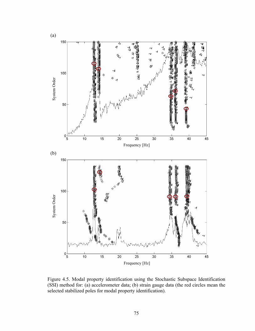
75
Figure 4.5. Modal property identification using the Stochastic Subspace Identification(SSI) method for: (a) accelerometer data; (b) strain gauge data (the red circles mean theselected stabilized poles for modal property identification).
(a)
(b)
Frequency [Hz]
Frequency [Hz]
Sys
tem
Ord
er
Sys
tem
Ord
er
76
vibration mode. Detailed comparisons of extracted mode shapes are presented in
Section 4.2.3.
By using the SSI method on the vibration response data from the white noise random
excitation tests, the lowest five vibration modes were extracted. The measured natural
frequencies of the system for various health states are presented and compared in
Section 4.2.3, while the corresponding mode shapes are described in Section 4.2.4.
After the natural frequencies had been identified, harmonic excitation was applied at
each individual natural frequency to permit accurate measurement of the corresponding
mode shapes. Figure 4.6 shows a typical vibration response to harmonic excitation for
the data from the reference accelerometer, where Fig. 4.6 (a) shows the acceleration
time history and Fig. 4.6 (b) presents the corresponding frequency spectrum. The signal
shown in Fig. 4.6 (a) came from the reference accelerometer channel during the tests for
Health State 1 (i.e., the intact condition) when the model was excited by harmonic
loading at the first natural frequency, as identified during the white noise random
excitation tests. Figure 4.7 presents a typical vibration response to harmonic excitation
for the data from a bottom strain gauge under identical testing conditions. Both Fig. 4.6
(b) and Fig. 4.7 (b) show only one apparent and dominant peak, which implies that
using the simple PP method can produce a highly repeatable mode shape definition. As
a result, the PP method was adopted to process the data with harmonic excitation. The
measured first and second mode shapes using harmonic excitation for various health
states are presented and compared in Section 4.2.4.
4.2.2 Measured natural frequencies
The lowest five natural frequencies of the bridge model in Health State 1, extracted from
both the accelerometer and strain gauge data in five trials, as obtained using the white
noise random excitation, are listed in Table 4.1 and Table 4.2, respectively. To define
one vibration mode, each trial requires five setups for accelerometer data while only one
setup was required for strain gauge data. One set of data could generate one natural
frequency value for each mode using the SSI modal analysis method (i.e., for each
individual vibration mode, one common natural frequency could be generated from each

77
set of data recorded by either seven accelerometers or 57 strain gauges). As a result,
Table 4.1 shows 25 different natural frequencies for each vibration mode from 25 sets of
data (five trials of five setups). The averaged frequencies from the five different setups
are also listed in Table 4.1 for each individual trial and each individual mode. The
averaged frequency, the standard deviation, and the corresponding coefficient of
variation, of all measured frequencies from the 25 sets of data, are also presented in
Table 4.1 for each individual mode. In a similar manner, Table 4.2 lists the results of
Figure 4.6. Closer view of acceleration response to harmonic excitation at the 1st modefor the reference accelerometer in Health State 1: (a) acceleration time history (a onesecond segment of the signal); (b) acceleration spectrum (frequency range showing upto 50 Hz).
(a)
(b)
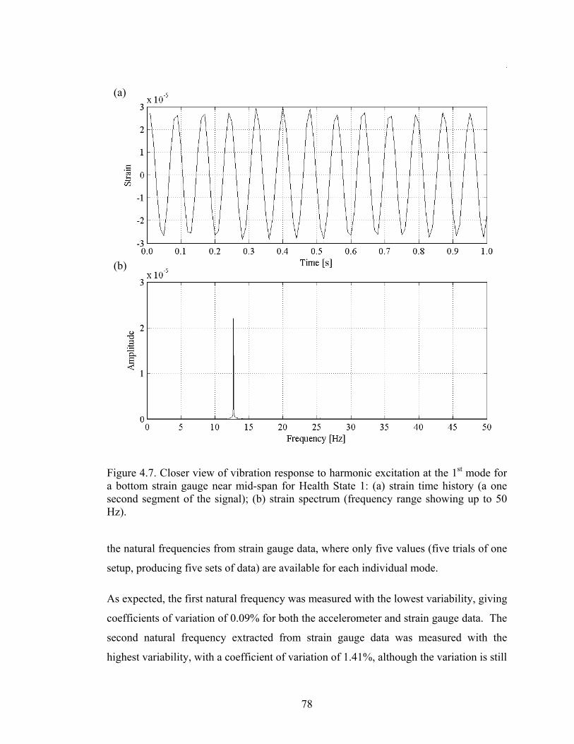
78
the natural frequencies from strain gauge data, where only five values (five trials of one
setup, producing five sets of data) are available for each individual mode.
As expected, the first natural frequency was measured with the lowest variability, giving
coefficients of variation of 0.09% for both the accelerometer and strain gauge data. The
second natural frequency extracted from strain gauge data was measured with the
highest variability, with a coefficient of variation of 1.41%, although the variation is still
Figure 4.7. Closer view of vibration response to harmonic excitation at the 1st mode fora bottom strain gauge near mid-span for Health State 1: (a) strain time history (a onesecond segment of the signal); (b) strain spectrum (frequency range showing up to 50Hz).
(a)
(b)

79
Table 4.1. Measured natural frequencies using accelerometers for Health State 1.
Trials Setups
Measured natural frequency (Hz)
Mode 1 Mode 2 Mode 3 Mode 4 Mode 5
Trial 1
Set 1_1 12.700 13.871 34.656 36.043 39.133 Set 2_1 12.689 13.884 34.557 35.973 38.841 Set 3_1 12.693 13.901 34.445 35.879 38.829 Set 4_1 12.693 13.892 34.537 35.845 38.719 Set 5_1 12.680 13.858 34.580 35.804 38.830
Average (Hz) 12.691 13.881 34.555 35.909 38.871
Trial 2
Set 1_2 12.719 13.876 34.679 35.945 39.147 Set 2_2 12.708 13.891 34.582 35.881 38.799 Set 3_2 12.696 13.914 34.486 35.908 38.722 Set 4_2 12.705 13.885 34.555 35.874 38.717 Set 5_2 12.679 13.871 34.523 35.815 38.730
Average (Hz) 12.701 13.888 34.565 35.885 38.823
Trial 3
Set 1_3 12.711 13.876 34.664 35.958 39.051 Set 2_3 12.706 13.895 34.588 36.035 38.798 Set 3_3 12.701 13.893 34.485 35.788 38.625 Set 4_3 12.697 13.867 34.503 35.805 38.787 Set 5_3 12.682 13.861 34.539 35.822 38.735
Average (Hz) 12.699 13.878 34.556 35.882 38.799
Trial 4
Set 1_4 12.712 13.918 34.701 35.957 39.122 Set 2_4 12.697 13.892 34.548 35.926 38.798 Set 3_4 12.706 13.906 34.534 35.790 38.771 Set 4_4 12.699 13.903 34.561 35.884 38.763 Set 5_4 12.688 13.858 34.486 35.795 38.742
Average (Hz) 12.700 13.896 34.566 35.870 38.839
Trial 5
Set 1_5 12.701 13.879 34.636 35.990 39.157 Set 2_5 12.694 13.895 34.554 35.926 38.737 Set 3_5 12.718 13.915 34.464 35.940 38.825 Set 4_5 12.686 13.889 34.530 35.886 38.709 Set 5_5 12.683 13.864 34.509 35.819 38.688
Average (Hz) 12.696 13.888 34.539 35.912 38.823
All Data Average (Hz) 12.698 13.886 34.556 35.892 38.831 STDEV (Hz) 0.011 0.018 0.068 0.077 0.157
C.O.V. 0.09% 0.13% 0.20% 0.21% 0.41% STDEV = Standard deviation; C.O.V. = Coefficient of variation.
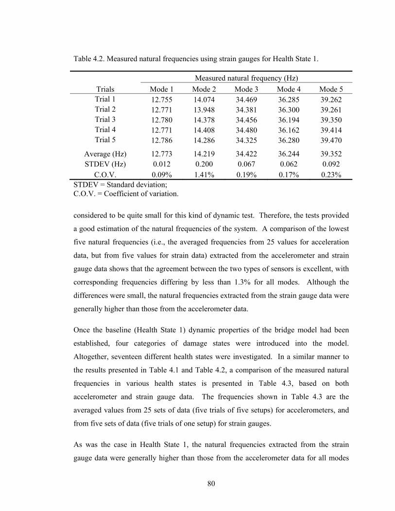
80
considered to be quite small for this kind of dynamic test. Therefore, the tests provided
a good estimation of the natural frequencies of the system. A comparison of the lowest
five natural frequencies (i.e., the averaged frequencies from 25 values for acceleration
data, but from five values for strain data) extracted from the accelerometer and strain
gauge data shows that the agreement between the two types of sensors is excellent, with
corresponding frequencies differing by less than 1.3% for all modes. Although the
differences were small, the natural frequencies extracted from the strain gauge data were
generally higher than those from the accelerometer data.
Once the baseline (Health State 1) dynamic properties of the bridge model had been
established, four categories of damage states were introduced into the model.
Altogether, seventeen different health states were investigated. In a similar manner to
the results presented in Table 4.1 and Table 4.2, a comparison of the measured natural
frequencies in various health states is presented in Table 4.3, based on both
accelerometer and strain gauge data. The frequencies shown in Table 4.3 are the
averaged values from 25 sets of data (five trials of five setups) for accelerometers, and
from five sets of data (five trials of one setup) for strain gauges.
As was the case in Health State 1, the natural frequencies extracted from the strain
gauge data were generally higher than those from the accelerometer data for all modes
Table 4.2. Measured natural frequencies using strain gauges for Health State 1.
Trials
Measured natural frequency (Hz)
Mode 1 Mode 2 Mode 3 Mode 4 Mode 5 Trial 1 12.755 14.074 34.469 36.285 39.262 Trial 2 12.771 13.948 34.381 36.300 39.261 Trial 3 12.780 14.378 34.456 36.194 39.350 Trial 4 12.771 14.408 34.480 36.162 39.414 Trial 5 12.786 14.286 34.325 36.280 39.470
Average (Hz) 12.773 14.219 34.422 36.244 39.352 STDEV (Hz) 0.012 0.200 0.067 0.062 0.092
C.O.V. 0.09% 1.41% 0.19% 0.17% 0.23% STDEV = Standard deviation; C.O.V. = Coefficient of variation.
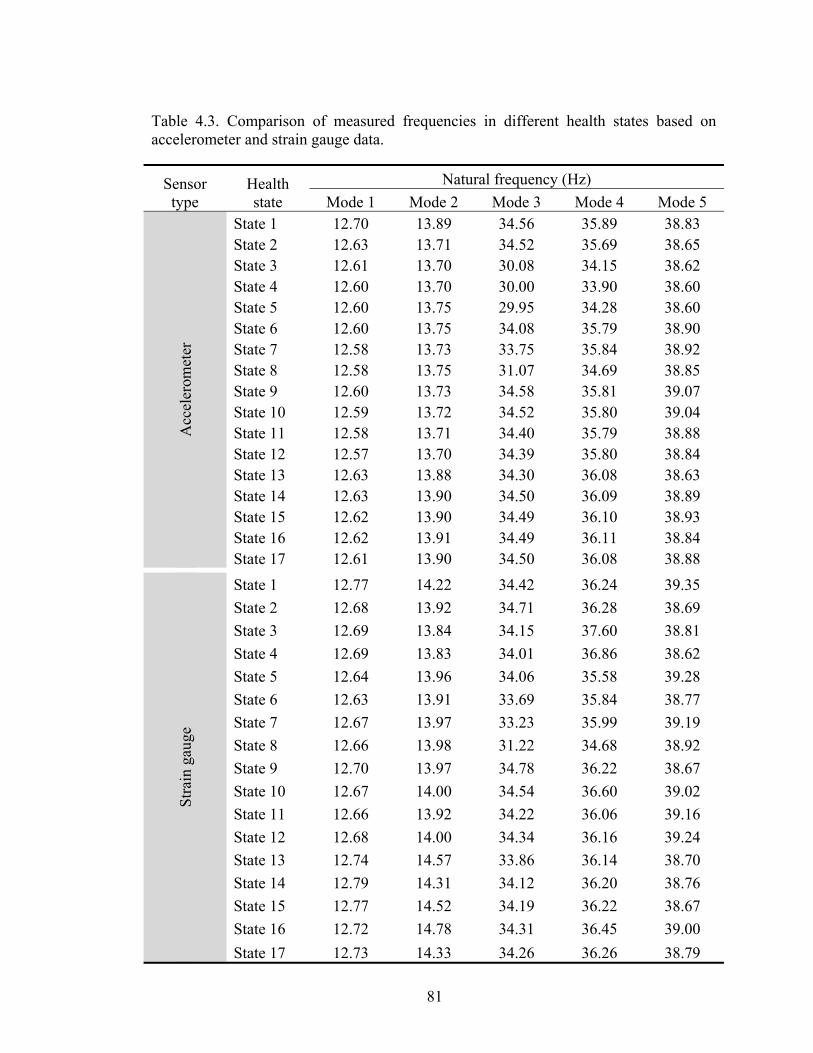
81
Table 4.3. Comparison of measured frequencies in different health states based on accelerometer and strain gauge data.
Sensor type
Health state
Natural frequency (Hz)
Mode 1 Mode 2 Mode 3 Mode 4 Mode 5 A
ccel
erom
eter
State 1 12.70 13.89 34.56 35.89 38.83 State 2 12.63 13.71 34.52 35.69 38.65 State 3 12.61 13.70 30.08 34.15 38.62 State 4 12.60 13.70 30.00 33.90 38.60 State 5 12.60 13.75 29.95 34.28 38.60 State 6 12.60 13.75 34.08 35.79 38.90 State 7 12.58 13.73 33.75 35.84 38.92 State 8 12.58 13.75 31.07 34.69 38.85 State 9 12.60 13.73 34.58 35.81 39.07 State 10 12.59 13.72 34.52 35.80 39.04 State 11 12.58 13.71 34.40 35.79 38.88 State 12 12.57 13.70 34.39 35.80 38.84 State 13 12.63 13.88 34.30 36.08 38.63 State 14 12.63 13.90 34.50 36.09 38.89 State 15 12.62 13.90 34.49 36.10 38.93 State 16 12.62 13.91 34.49 36.11 38.84 State 17 12.61 13.90 34.50 36.08 38.88
Str
ain
gaug
e
State 1 12.77 14.22 34.42 36.24 39.35
State 2 12.68 13.92 34.71 36.28 38.69
State 3 12.69 13.84 34.15 37.60 38.81
State 4 12.69 13.83 34.01 36.86 38.62
State 5 12.64 13.96 34.06 35.58 39.28
State 6 12.63 13.91 33.69 35.84 38.77
State 7 12.67 13.97 33.23 35.99 39.19
State 8 12.66 13.98 31.22 34.68 38.92
State 9 12.70 13.97 34.78 36.22 38.67
State 10 12.67 14.00 34.54 36.60 39.02
State 11 12.66 13.92 34.22 36.06 39.16
State 12 12.68 14.00 34.34 36.16 39.24
State 13 12.74 14.57 33.86 36.14 38.70
State 14 12.79 14.31 34.12 36.20 38.76
State 15 12.77 14.52 34.19 36.22 38.67
State 16 12.72 14.78 34.31 36.45 39.00
State 17 12.73 14.33 34.26 36.26 38.79

82
in all health states. The maximum change in the fundamental natural frequency among
various health states was relatively small, 0.98% and 1.26% for the frequencies
extracted from accelerometer and strain gauge data, respectively. The small changes
imply that the change in fundamental natural frequency may not be a sensitive damage
indicator, particularly when considering environmental effects experienced by a real
structure. The maximum change in the frequency of Mode 5 (the second flexural mode
shape, as seen in the next section) among various health states was also relatively small,
at 1.20% and 1.86% for the frequency extracted from accelerometer and strain gauge
data, respectively.
On the other hand, the maximum change in the frequency of Mode 3 among various
health states was relatively large, at 13.37% and 10.23% for the frequency extracted
from accelerometer and strain gauge data, respectively. In fact, for accelerometer data,
the frequency of Mode 3 (around 30 Hz) in several health states, including Health States
3, 4, 5, and 8, was significantly different from the corresponding frequency in other
health states (around 34 Hz). The common feature of the Health States 3, 4, 5, and 8
(see Table 3.4) was that one cross-bracing diaphragm located around the mid-span of
the bridge (i.e., D-X5.2Y2.25 or D-X2.8Y1.35, see Fig. 3.3) was disconnected, which
could reduce the lateral and torsional stiffness of the structure significantly.
The largest changes in frequency were found to result from shifts in modes (i.e., the
mode shifts to another different mode due to the presence of damage, which means that
the two modes compared may be treated as two different modes) instead of changes in
the same mode. In other words, a completely different new mode shape (i.e., Mode 3
with a frequency around 30 Hz) was introduced for the Health States 3, 4, 5, and 8, due
to the disconnection of the cross-bracing diaphragms around mid-span of the bridge.
Mode 4 in these health states is most likely similar to Mode 3 in other health states,
while the vibration mode around 35.8 Hz (similar to Mode 4 in other health states)
either disappeared or was inadvertently not extracted since the modes were so close to
each other and five other modes had already been detected. For strain gauge data, there
are similar results for Health State 8 (with frequency of 31.22 Hz). However, the lower
frequency mode (around 30 Hz) in Health States 3, 4, and 5 was not extracted, which

83
may be due to the fact that the strain gauges were not sensitive to the higher frequency
signals; also, the vibration mode around 30 Hz did not appear to be as dominant in these
health states.
Although comparison of two different modes may be meaningless in one sense, from
another perspective, it could be very useful because the large shifting in modes could be
a good indicator for global damage. For example, in the current study, the
disconnection of cross-bracing diaphragms changed the load sharing between different
girders, hence the global stiffness, and ultimately the resulting torsional modes.
4.2.3 Measured mode shapes
Mode shapes for the lowest five vibration modes of the intact (i.e., Health State 1)
bridge model, as derived from accelerometer and strain gauge data, are presented in
Figures 4.8 and 4.9, respectively. In both cases, the mode shapes were averaged from
five unit-area normalized mode shapes (see Section 4.4.3), which were extracted from
data recorded in five repeated tests, each with a recorded period of 80 seconds, using
white noise random excitation. The strain-based mode shapes represent the relative
magnitudes of modal strain responses measured at the lowest of the three strain gauges
at each instrumented location.
It should be acknowledged that the strain-based mode shapes are somewhat different
from the traditional definition of mode shape using deflection. Actually, the strain-
based mode shape is directly related to the curvature of the deflection mode shape,
based on the assumption that the location of the neutral axis remains constant both in
tension and compression under small deflections and that the structure remains in a
linear elastic state. However, the change in strain-based mode shapes can still be used
in structural health monitoring, whether or not this assumption is correct. This is
because the strain gauges were permanently installed, and therefore the locations and
conditions of sensors were consistent between various tests. As a result, any change in
the physical condition of the structure (reflecting its stiffness and load capacity) should
be reflected in the strain gauge measurements.
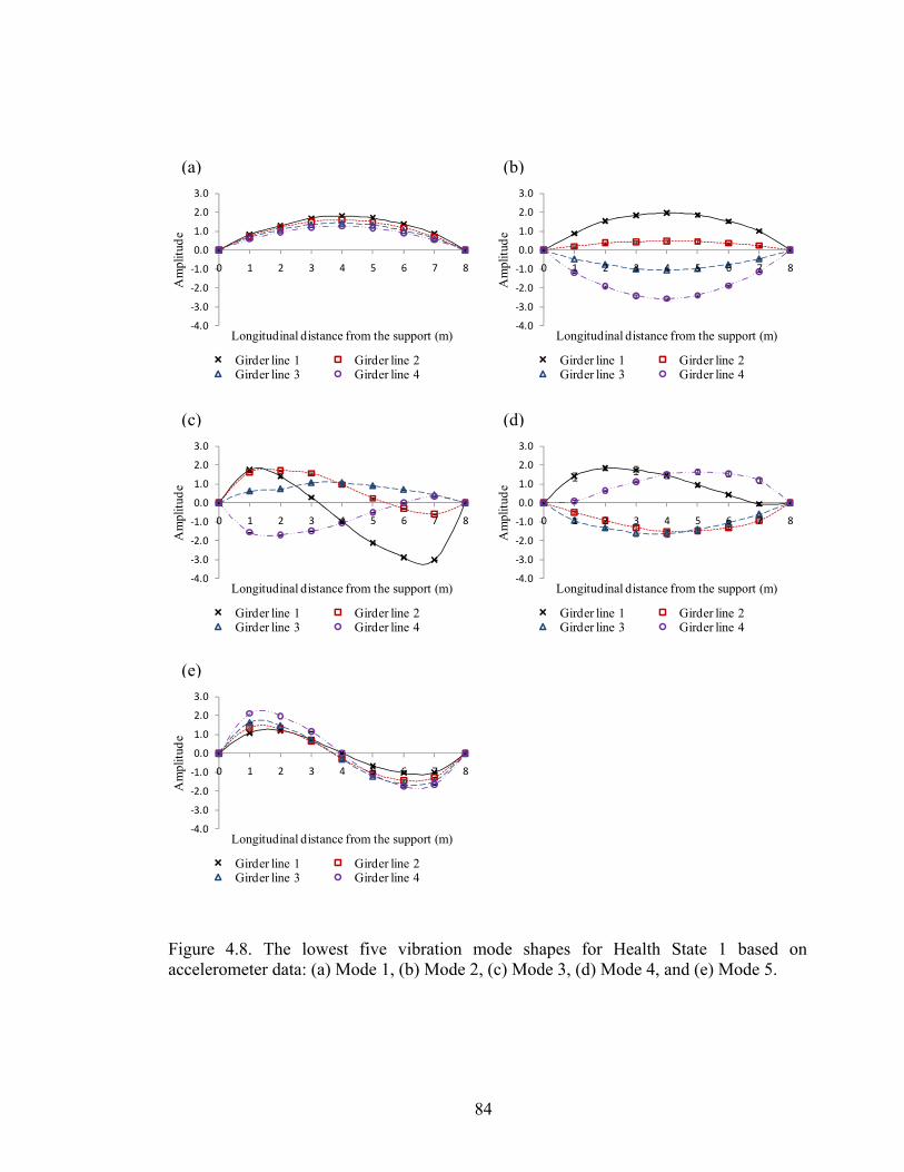
84
Figure 4.8. The lowest five vibration mode shapes for Health State 1 based onaccelerometer data: (a) Mode 1, (b) Mode 2, (c) Mode 3, (d) Mode 4, and (e) Mode 5.
(a) (b)
(c) (d)
(e)
‐4.0
‐3.0
‐2.0
‐1.0
0.0
1.0
2.0
3.0
0 1 2 3 4 5 6 7 8
Am
plit
ude
Longitudinal distance from the support (m)
Girder line 1 Girder line 2Girder line 3 Girder line 4
‐4.0
‐3.0
‐2.0
‐1.0
0.0
1.0
2.0
3.0
0 1 2 3 4 5 6 7 8
Am
plit
ude
Longitudinal distance from the support (m)
Girder line 1 Girder line 2Girder line 3 Girder line 4
‐4.0
‐3.0
‐2.0
‐1.0
0.0
1.0
2.0
3.0
0 1 2 3 4 5 6 7 8
Am
plit
ude
Longitudinal distance from the support (m)
Girder line 1 Girder line 2Girder line 3 Girder line 4
‐4.0
‐3.0
‐2.0
‐1.0
0.0
1.0
2.0
3.0
0 1 2 3 4 5 6 7 8
Am
plit
ude
Longitudinal distance from the support (m)
Girder line 1 Girder line 2Girder line 3 Girder line 4
‐4.0
‐3.0
‐2.0
‐1.0
0.0
1.0
2.0
3.0
0 1 2 3 4 5 6 7 8
Am
plit
ude
Longitudinal distance from the support (m)
Girder line 1 Girder line 2Girder line 3 Girder line 4

85
Figure 4.9. The lowest five vibration mode shapes for Health State 1 based on bottomstrain gauge data: (a) Mode 1, (b) Mode 2, (c) Mode 3, (d) Mode 4, and (e) Mode 5.
(b)
(d)
‐4.0
‐3.0
‐2.0
‐1.0
0.0
1.0
2.0
3.0
0 1 2 3 4 5 6 7 8
Am
plit
ude
Longitudinal distance from the support (m)
Girder line 1 Girder line 2Girder line 3 Girder line 4
‐4.0
‐3.0
‐2.0
‐1.0
0.0
1.0
2.0
3.0
0 1 2 3 4 5 6 7 8
Am
plit
ude
Longitudinal distance from the support (m)
Girder line 1 Girder line 2Girder line 3 Girder line 4
‐4.0
‐3.0
‐2.0
‐1.0
0.0
1.0
2.0
3.0
0 1 2 3 4 5 6 7 8
Am
plit
ude
Longitudinal distance from the support (m)
Girder line 1 Girder line 2Girder line 3 Girder line 4
‐4.0
‐3.0
‐2.0
‐1.0
0.0
1.0
2.0
3.0
4.0
0 1 2 3 4 5 6 7 8Am
plit
ude
Longitudinal distance from the support (m)
Girder line 1 Girder line 2Girder line 3 Girder line 4
‐4.0
‐3.0
‐2.0
‐1.0
0.0
1.0
2.0
3.0
0 1 2 3 4 5 6 7 8
Am
plit
ude
Longitudinal distance from the support (m)
Girder line 1 Girder line 2Girder line 3 Girder line 4
(c)
(a)
(e)
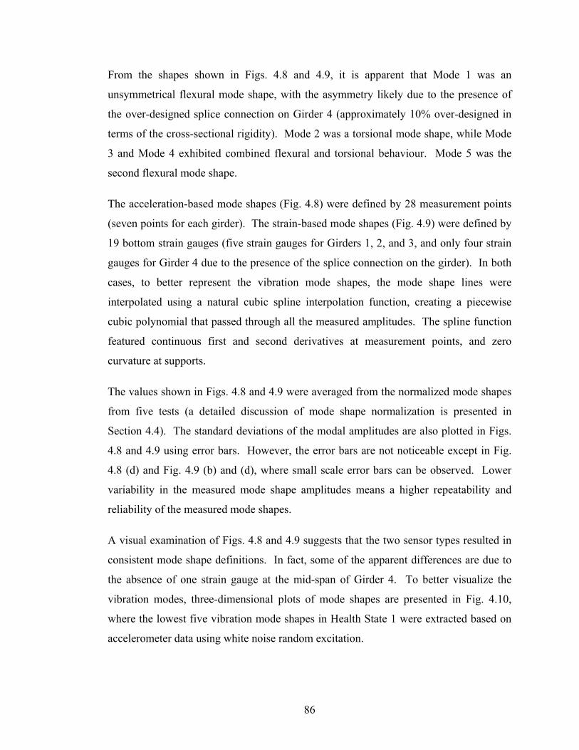
86
From the shapes shown in Figs. 4.8 and 4.9, it is apparent that Mode 1 was an
unsymmetrical flexural mode shape, with the asymmetry likely due to the presence of
the over-designed splice connection on Girder 4 (approximately 10% over-designed in
terms of the cross-sectional rigidity). Mode 2 was a torsional mode shape, while Mode
3 and Mode 4 exhibited combined flexural and torsional behaviour. Mode 5 was the
second flexural mode shape.
The acceleration-based mode shapes (Fig. 4.8) were defined by 28 measurement points
(seven points for each girder). The strain-based mode shapes (Fig. 4.9) were defined by
19 bottom strain gauges (five strain gauges for Girders 1, 2, and 3, and only four strain
gauges for Girder 4 due to the presence of the splice connection on the girder). In both
cases, to better represent the vibration mode shapes, the mode shape lines were
interpolated using a natural cubic spline interpolation function, creating a piecewise
cubic polynomial that passed through all the measured amplitudes. The spline function
featured continuous first and second derivatives at measurement points, and zero
curvature at supports.
The values shown in Figs. 4.8 and 4.9 were averaged from the normalized mode shapes
from five tests (a detailed discussion of mode shape normalization is presented in
Section 4.4). The standard deviations of the modal amplitudes are also plotted in Figs.
4.8 and 4.9 using error bars. However, the error bars are not noticeable except in Fig.
4.8 (d) and Fig. 4.9 (b) and (d), where small scale error bars can be observed. Lower
variability in the measured mode shape amplitudes means a higher repeatability and
reliability of the measured mode shapes.
A visual examination of Figs. 4.8 and 4.9 suggests that the two sensor types resulted in
consistent mode shape definitions. In fact, some of the apparent differences are due to
the absence of one strain gauge at the mid-span of Girder 4. To better visualize the
vibration modes, three-dimensional plots of mode shapes are presented in Fig. 4.10,
where the lowest five vibration mode shapes in Health State 1 were extracted based on
accelerometer data using white noise random excitation.

87
00.9
1.82.7
‐0.5
0.0
0.5
1.0
1.5
2.0
01
23
45
67
8
Figure 4.10. The lowest five vibration mode shapes for Health State 1 based onaccelerometer data with white noise random excitation: (a) Mode 1, (b) Mode 2, (c)Mode 3, (d) Mode 4, and (e) Mode 5.
(a) (b)
(c) (d)
(e)
00.9
1.82.7
‐4.0
‐2.0
0.0
2.00
12
34
56
78
00.9
1.82.7
‐4.0
‐2.0
0.0
2.00
12
34
56
78
00.9
1.82.7
‐2.0
‐1.0
0.0
1.0
2.0
01
23
45
67
8
00.9
1.82.7
‐2.0
0.0
2.0
4.0
01
23
45
67
8

88
4.2.4 Comparison of the measured mode shapes in different health states
A comparison of the first and second mode shapes measured for different health states is
presented in Figs. 4.11 and 4.12. In all cases, the vibration mode shapes shown were
averaged from the normalized modal amplitudes using a unit-area normalization method
(see Section 4.4.3), extracted from the accelerometer data of five repeated tests, using
harmonic excitation. These are slightly different from the mode shapes defined in Fig.
4.8, where white noise excitation was used. To better compare the results, the mode
shapes corresponding to different health states have been divided into four groups and
presented in four plots, with the mode shape for Health State 1 appearing in each plot as
a common reference. Also, to improve the clarity in each plot, the mode shapes along
individual girder lines have been separated and strung end to end.
A visual examination of Figs. 4.11 and 4.12 demonstrates that the mode shapes in
different health states were very similar, although some differences in mode shape
amplitudes are noticeable for some health states. The major noticeable differences were
due to the disconnection (Health State 2) or re-connection (Health State 13) of the splice
on Girder 4. Quantitative comparisons of mode shapes are available in Chapter 6.
Additional information about the definition of other mode shapes is available in
Appendix E.
4.3 Influence of Test Parameters on Dynamic Properties
4.3.1 Overview
Since VBDD methods rely on the identification of small changes in dynamic properties
to infer the nature of the damage, reliable estimates of these properties are essential for a
successful implementation of VBDD schemes. As a result, the influence of various
testing parameters on the repeatability and reliability of modal property extraction was
investigated on the intact bridge model (i.e., Health State 1, see Section 3.4) in Phase I
of the dynamic tests (see Table 3.1). To simplify the process, only the sensors located
on Girder 1 were used for this investigation. More specifically, the testing parameters
investigated in this study included sensor type and vertical location of strain gauges,
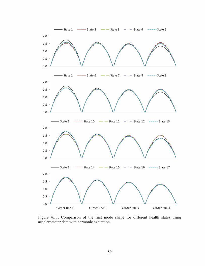
89
0.0
0.5
1.0
1.5
2.0
State 1 State 14 State 15 State 16 State 17
Figure 4.11. Comparison of the first mode shape for different health states usingaccelerometer data with harmonic excitation.
Girder line 1 Girder line 2 Girder line 3 Girder line 4
0.0
0.5
1.0
1.5
2.0
State 1 State 2 State 3 State 4 State 5
0.0
0.5
1.0
1.5
2.0
State 1 State 6 State 7 State 8 State 9
0.0
0.5
1.0
1.5
2.0
State 1 State 10 State 11 State 12 State 13
90
‐4.0
‐2.0
0.0
2.0
4.0
State 1 State 14 State 15 State 16 State 17
Figure 4.12. Comparison of the second mode shape for different health states usingaccelerometer data with harmonic excitation.
Girder line 1 Girder line 2 Girder line 3 Girder line 4
‐4.0
‐2.0
0.0
2.0
4.0
State 1 State 2 State 3 State 4 State 5
‐4.0
‐2.0
0.0
2.0
4.0
State 1 State 6 State 7 State 8 State 9
‐4.0
‐2.0
0.0
2.0
4.0
State 1 State 10 State 11 State 12 State 13

91
excitation methods, data sampling period (the length in time of recorded signal), modal
analysis method, and data sampling rates.
4.3.2 Influence of sensor type and vertical location of strain gauges
The lowest five vibration mode shapes along Girder 1 of the intact bridge model were
extracted using the SSI method from accelerometer and strain gauge data, where data
from three separate groups of strain gauges were considered as individual cases,
corresponding to data from only the bottom, middle, or top strain gauges at all locations.
The data were recorded for a period of 80 seconds with a sampling rate of 1000 Hz,
under white noise random excitation. Before using the SSI method to identify the modal
properties, the recorded signals were decimated to a lower sampling rate of 200 Hz
using low-pass digital filter techniques. A quantitative comparison of the mode shapes
is summarized in Table 4.4 according to the four groups of sensors used to define the
mode shapes. Here, the mode shapes are compared based on the Modal Assurance
Criteria (MAC) (Ewins 2000), defined as:
∑ ∙
∑ ∙ ∑ [4.1]
where and are two mode shape vectors being compared, the subscript indicates
an element in the vectors (corresponding to a particular sensor location), and
represents the number of measurement points. The MAC value represents the degree of
correlation between two mode shapes and varies from zero to unity. A MAC value of
unity denotes perfectly correlated mode shapes, while a MAC value of zero would
suggest a complete lack of correlation (i.e., orthogonal shapes).
As suggested above, in addition to mode shapes based on accelerometer readings,
results in Table 4.4 are also provided for mode shapes defined by the three groups of
strain gauges considered (the bottom, middle and top strain gauges at each instrumented
location). For all of these, MAC values provided in Table 4.4 represent averaged
comparisons between unit-norm normalized mode shapes (see Section 4.4.2), extracted
from individual trials and the averaged normalized mode shape generated from all five

92
trials for a given group of sensors. To clarify, first, the individual mode shapes were
extracted from the sensor data for five repeated trials. Then, the averaged mode shape
was calculated from the five extracted, individually unit-norm normalized mode shapes.
Next, the averaged mode shape was normalized again using unit-norm normalization.
Next, MAC values were calculated for each individual mode shape by comparing the
individual normalized mode shape and the averaged normalized mode shape using Eq.
4.1. Finally, the averaged MAC values were calculated from the five individual MAC
values for each sensor group and each vibration mode.
Overall, the accelerometer data produced the most reliable mode shape estimates, with
averaged MAC values exceeding 0.995 for all of the lowest five modes, and an averaged
MAC value exceeding 0.99999 for the fundamental mode, together with the lowest
coefficient of variation of 0.00032%. As expected, the bottom gauges provided the
most reliable results among the strain gauge groups, with averaged MAC values
(exceeding 0.9998 for the fundamental mode with coefficient of variation of 0.00662%)
only slightly lower than those based on accelerometer readings. The consistent trend of
deteriorating reliability as the gauges moved up toward the neutral axis illustrates the
role of the signal-to-noise ratio in the resulting uncertainty in measured mode shapes.
The comparable quality of the bottom strain gauge and accelerometer results, though,
suggests that the less expensive strain gauges may be a viable option for dynamic
Table 4.4. Influence of sensor group on mode shape reliability based on averaged MAC values from five repeated trials with white noise random excitation.
Instrumentation Mode 1 Mode 2 Mode 3 Mode 4 Mode 5
Acceleration Avg. 0.9999968 0.9995244 0.9998721 0.9958494 0.9997260C.O.V. 0.00032% 0.04091% 0.01181% 0.46720% 0.02529%
Bottom Strain Avg. 0.9998726 0.9977945 0.9991574 0.9940285 0.9982590C.O.V. 0.00662% 0.13401% 0.03676% 0.32077% 0.13412%
Middle Strain Avg. 0.9994881 0.9939806 0.9991072 0.9936696 0.9977089C.O.V. 0.04697% 0.50404% 0.04621% 0.34150% 0.15767%
Top Strain Avg. 0.9992558 0.9850748 0.9987266 0.9899599 0.9956863
C.O.V. 0.04638% 1.11304% 0.07789% 0.65779% 0.18205%
Avg. = Average; C.O.V. = Coefficient of variation.

93
system identification as long as the reliability of the measured signal can be maintained
at a sufficiently high level. However, mode shapes discussed in subsequent sub-sections
in Section 4.3 were based exclusively on accelerometer data.
4.3.3 Influence of excitation type
As described previously, both resonant harmonic and white noise random inputs were
used to excite the bridge model. A comparison of the mode shape reliability for the two
types of excitation is provided in Table 4.5. As described in the previous sub-section,
MAC results presented here represent averaged comparisons between unit-norm
normalized mode shapes extracted from individual trials and the averaged normalized
mode shape generated from all five trials using accelerometer data. Results using strain
gauge data are presented in Appendix E. The data were recorded for a period of 80
seconds for both white noise random and harmonic excitations. The data sampling rate
was 1000 Hz for white noise random excitation, then decimated to a lower sampling rate
of 200 Hz before using the SSI method to identify the modal properties. However, a
lower sampling rate of 500 Hz was used to record the data for harmonic excitation (due
to less uncertainty), which was then decimated to 100 Hz for modal identification using
the SSI method. For the harmonic loading trials, preliminary tests using random
excitation were required to identify system natural frequencies; for the random loading
trials, on the other hand, all modal parameters were extracted simultaneously from the
same data sets.
Table 4.5. Influence of excitation type on mode shape reliability based on averaged MAC values using accelerometer data from five replicate trials.
Excitation Mode 1 Mode 2 Mode 3 Mode 4 Mode 5
White Noise Avg. 0.9999968 0.9995244 0.9998721 0.9958494 0.9997260C.O.V. 0.00032% 0.04091% 0.01181% 0.46720% 0.02529%
Harmonic Avg. 1.0000000 0.9999997 0.9999861 0.9999935 0.9999588
C.O.V. 0.00000% 0.00004% 0.00110% 0.00049% 0.00488%
Avg. = Average; C.O.V. = Coefficient of variation.

94
As demonstrated in Table 4.5, resonant harmonic loading produced mode shapes with
exceptionally high repeatability (i.e., a MAC value greater than 0.99999999 for the
fundamental mode and greater than 0.9999 for all of the lowest five modes, with a
coefficient of variation less than 0.005% for all of the five modes). Results using white
noise random excitation were decidedly more uncertain, with MAC values as low as
0.995 for some modes, and a coefficient of variation as high as 0.467%.
4.3.4 Influence of recording period and modal analysis method
Based on random process theory, it may be expected that the detrimental effects of
random measurement and signal processing errors may be attenuated by making use of
longer measurement records in the estimation of modal properties. To help quantify the
extent of such benefits, a series of trials was carried out featuring five different sampling
periods ranging from 10 s to 160 s in length (i.e., from 128 to 2044 times the
fundamental period). First, five trials were carried out for each sampling period, using a
sampling frequency of 200 Hz when both harmonic and white noise random excitations
were used. Then, the same process was carried out using a sampling rate of 1000 Hz for
white noise random excitation only.
For resonant harmonic excitation using a sampling rate of 200 Hz (then decimated to
100 Hz in data pre-processing), the measured fundamental mode shapes for various
sampling periods (from 10 s to 160 s) are presented in Figure 4.13, where both the SSI
and PP methods were used to extract modal properties. As before, the mode shapes
presented in Fig. 4.13 were averaged from five unit-norm normalized mode shapes. The
standard deviations of the amplitudes of mode shapes from five trials are also plotted in
the figure using error bars. However, the error bars are not noticeable visually for any
of the sampling periods no matter which modal analysis method was adopted (i.e., SSI
or PP method), which suggests that the measured mode shapes are highly repeatable
with little variation even for a recording period as short as ten seconds. Also, it can be
seen from the results that the PP method resulted in a comparable accuracy of mode
shape definition compared with the SSI method. As a result, it was considered suitable
to use the simple and time-saving PP modal analysis method to extract modal properties

95
for Phase II vibration tests conducted later on (see Table 3.1) when using resonant
harmonic excitation.
A quantitative comparison of the fundamental mode shape repeatability for various
sampling periods, using the same mode shapes shown in Fig. 4.13, is presented in Table
4.6. As before, the averaged MAC values in Table 4.6 were calculated from five
individual MAC values that represent a comparison between the normalized mode shape
extracted from a single trial under a specific set of conditions (i.e., excitation type and
sampling period) and the averaged normalized mode shape computed for all five trials
0.0
0.1
0.2
0.3
0.4
0.5
0.6
0.7
0 1 2 3 4 5 6 7 8Nor
mal
ized
Mod
al A
mpl
itud
e
Longitudinal distance from the left support (m)
10s_PP
20s_PP
40s_PP
80s_PP
160s_PP
0.0
0.1
0.2
0.3
0.4
0.5
0.6
0.7
0 1 2 3 4 5 6 7 8Nor
mal
ized
Mod
al A
mpl
itud
e
Longitudinal distance from the left support (m)
10s_SSI
20s_SSI
40s_SSI
80s_SSI
160s_SSI
Figure 4.13. Influence of recording period on mode shape definition for resonantharmonic excitation when both (a) SSI and (b) PP methods were used to extract modalproperties.
(a)
(b)
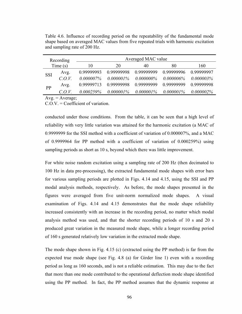
96
conducted under those conditions. From the table, it can be seen that a high level of
reliability with very little variation was attained for the harmonic excitation (a MAC of
0.9999999 for the SSI method with a coefficient of variation of 0.000007%, and a MAC
of 0.9999964 for PP method with a coefficient of variation of 0.000259%) using
sampling periods as short as 10 s, beyond which there was little improvement.
For white noise random excitation using a sampling rate of 200 Hz (then decimated to
100 Hz in data pre-processing), the extracted fundamental mode shapes with error bars
for various sampling periods are plotted in Figs. 4.14 and 4.15, using the SSI and PP
modal analysis methods, respectively. As before, the mode shapes presented in the
figures were averaged from five unit-norm normalized mode shapes. A visual
examination of Figs. 4.14 and 4.15 demonstrates that the mode shape reliability
increased consistently with an increase in the recording period, no matter which modal
analysis method was used, and that the shorter recording periods of 10 s and 20 s
produced great variation in the measured mode shape, while a longer recording period
of 160 s generated relatively low variation in the extracted mode shape.
The mode shape shown in Fig. 4.15 (c) (extracted using the PP method) is far from the
expected true mode shape (see Fig. 4.8 (a) for Girder line 1) even with a recording
period as long as 160 seconds, and is not a reliable estimation. This may due to the fact
that more than one mode contributed to the operational deflection mode shape identified
using the PP method. In fact, the PP method assumes that the dynamic response at
Table 4.6. Influence of recording period on the repeatability of the fundamental mode shape based on averaged MAC values from five repeated trials with harmonic excitation and sampling rate of 200 Hz.
Recording Time (s)
Averaged MAC value
10 20 40 80 160
SSI Avg. 0.99999993 0.99999998 0.99999999 0.99999996 0.99999997
C.O.V. 0.000007% 0.000001% 0.000000% 0.000006% 0.000003%
PP Avg. 0.99999713 0.99999998 0.99999999 0.99999999 0.99999998
C.O.V. 0.000259% 0.000001% 0.000001% 0.000001% 0.000002% Avg. = Average; C.O.V. = Coefficient of variation.

97
0.0
0.1
0.2
0.3
0.4
0.5
0.6
0.7
0 1 2 3 4 5 6 7 8Nor
mal
ized
Mod
al A
mpl
itud
e
Longitudinal distance from the left support (m)
160s_SSI
0.0
0.1
0.2
0.3
0.4
0.5
0.6
0.7
0 1 2 3 4 5 6 7 8Nor
mal
ized
Mod
al A
mpl
itud
e
Longitudinal distance from the left support (m)
40s_SSI
80s_SSI
0.0
0.1
0.2
0.3
0.4
0.5
0.6
0.7
0 1 2 3 4 5 6 7 8Nor
mal
ized
Mod
al A
mpl
itud
e
Longitudinal distance from the left support (m)
10s_SSI
20s_SSI
Figure 4.14. Influence of recording period on mode shape definition for white noiserandom excitation with sampling rate of 200 Hz when the SSI method was used toextract modal properties.
(a)
(b)
(c)

98
0.0
0.1
0.2
0.3
0.4
0.5
0.6
0.7
0 1 2 3 4 5 6 7 8Nor
mal
ized
Mod
al A
mpl
itud
e
Longitudinal distance from the left support (m)
160s_PP
0.0
0.1
0.2
0.3
0.4
0.5
0.6
0.7
0 1 2 3 4 5 6 7 8Nor
mal
ized
Mod
al A
mpl
itud
e
Longitudinal distance from the left support (m)
40s_PP
80s_PP
0.0
0.1
0.2
0.3
0.4
0.5
0.6
0.7
0 1 2 3 4 5 6 7 8Nor
mal
ized
Mod
al A
mpl
itud
e
Longitudinal distance from the left support (m)
10s_PP
20s_PP
Figure 4.15. Influence of recording period on mode shape definition for white noiserandom excitation with sampling rate of 200 Hz when the PP method was used to extractmodal properties.
(a)
(b)
(c)
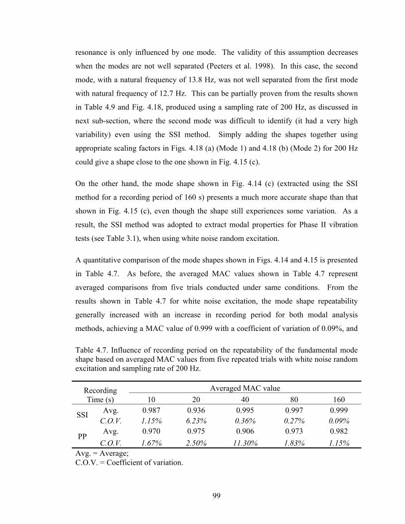
99
resonance is only influenced by one mode. The validity of this assumption decreases
when the modes are not well separated (Peeters et al. 1998). In this case, the second
mode, with a natural frequency of 13.8 Hz, was not well separated from the first mode
with natural frequency of 12.7 Hz. This can be partially proven from the results shown
in Table 4.9 and Fig. 4.18, produced using a sampling rate of 200 Hz, as discussed in
next sub-section, where the second mode was difficult to identify (it had a very high
variability) even using the SSI method. Simply adding the shapes together using
appropriate scaling factors in Figs. 4.18 (a) (Mode 1) and 4.18 (b) (Mode 2) for 200 Hz
could give a shape close to the one shown in Fig. 4.15 (c).
On the other hand, the mode shape shown in Fig. 4.14 (c) (extracted using the SSI
method for a recording period of 160 s) presents a much more accurate shape than that
shown in Fig. 4.15 (c), even though the shape still experiences some variation. As a
result, the SSI method was adopted to extract modal properties for Phase II vibration
tests (see Table 3.1), when using white noise random excitation.
A quantitative comparison of the mode shapes shown in Figs. 4.14 and 4.15 is presented
in Table 4.7. As before, the averaged MAC values shown in Table 4.7 represent
averaged comparisons from five trials conducted under same conditions. From the
results shown in Table 4.7 for white noise excitation, the mode shape repeatability
generally increased with an increase in recording period for both modal analysis
methods, achieving a MAC value of 0.999 with a coefficient of variation of 0.09%, and
Table 4.7. Influence of recording period on the repeatability of the fundamental mode shape based on averaged MAC values from five repeated trials with white noise random excitation and sampling rate of 200 Hz.
Recording Time (s)
Averaged MAC value
10 20 40 80 160
SSI Avg. 0.987 0.936 0.995 0.997 0.999
C.O.V. 1.15% 6.23% 0.36% 0.27% 0.09%
PP Avg. 0.970 0.975 0.906 0.973 0.982
C.O.V. 1.67% 2.50% 11.30% 1.83% 1.15% Avg. = Average; C.O.V. = Coefficient of variation.
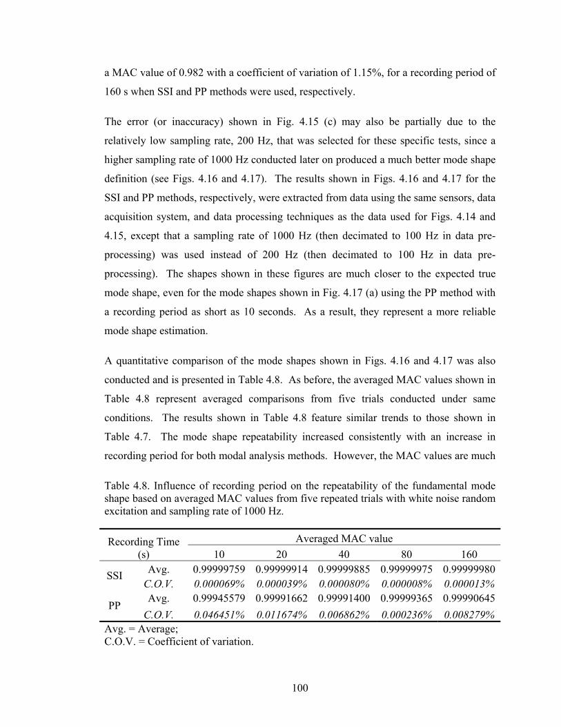
100
a MAC value of 0.982 with a coefficient of variation of 1.15%, for a recording period of
160 s when SSI and PP methods were used, respectively.
The error (or inaccuracy) shown in Fig. 4.15 (c) may also be partially due to the
relatively low sampling rate, 200 Hz, that was selected for these specific tests, since a
higher sampling rate of 1000 Hz conducted later on produced a much better mode shape
definition (see Figs. 4.16 and 4.17). The results shown in Figs. 4.16 and 4.17 for the
SSI and PP methods, respectively, were extracted from data using the same sensors, data
acquisition system, and data processing techniques as the data used for Figs. 4.14 and
4.15, except that a sampling rate of 1000 Hz (then decimated to 100 Hz in data pre-
processing) was used instead of 200 Hz (then decimated to 100 Hz in data pre-
processing). The shapes shown in these figures are much closer to the expected true
mode shape, even for the mode shapes shown in Fig. 4.17 (a) using the PP method with
a recording period as short as 10 seconds. As a result, they represent a more reliable
mode shape estimation.
A quantitative comparison of the mode shapes shown in Figs. 4.16 and 4.17 was also
conducted and is presented in Table 4.8. As before, the averaged MAC values shown in
Table 4.8 represent averaged comparisons from five trials conducted under same
conditions. The results shown in Table 4.8 feature similar trends to those shown in
Table 4.7. The mode shape repeatability increased consistently with an increase in
recording period for both modal analysis methods. However, the MAC values are much
Table 4.8. Influence of recording period on the repeatability of the fundamental mode shape based on averaged MAC values from five repeated trials with white noise random excitation and sampling rate of 1000 Hz.
Recording Time (s)
Averaged MAC value
10 20 40 80 160
SSI Avg. 0.99999759 0.99999914 0.99999885 0.99999975 0.99999980
C.O.V. 0.000069% 0.000039% 0.000080% 0.000008% 0.000013%
PP Avg. 0.99945579 0.99991662 0.99991400 0.99999365 0.99990645
C.O.V. 0.046451% 0.011674% 0.006862% 0.000236% 0.008279% Avg. = Average; C.O.V. = Coefficient of variation.

101
0.0
0.1
0.2
0.3
0.4
0.5
0.6
0.7
0 1 2 3 4 5 6 7 8Nor
mal
ized
Mod
al A
mpl
itud
e
Longitudinal distance from the left support (m)
160s_SSI
0.0
0.1
0.2
0.3
0.4
0.5
0.6
0.7
0 1 2 3 4 5 6 7 8Nor
mal
ized
Mod
al A
mpl
itud
e
Longitudinal distance from the left support (m)
40s_SSI
80s_SSI
0.0
0.1
0.2
0.3
0.4
0.5
0.6
0.7
0 1 2 3 4 5 6 7 8Nor
mal
ized
Mod
al A
mpl
itud
e
Longitudinal distance from the left support (m)
10s_SSI
20s_SSI
Figure 4.16. Influence of recording period on mode shape definition for white noiserandom excitation with sampling rate of 1000 Hz when SSI method was used to extractmodal properties.
(a)
(b)
(c)
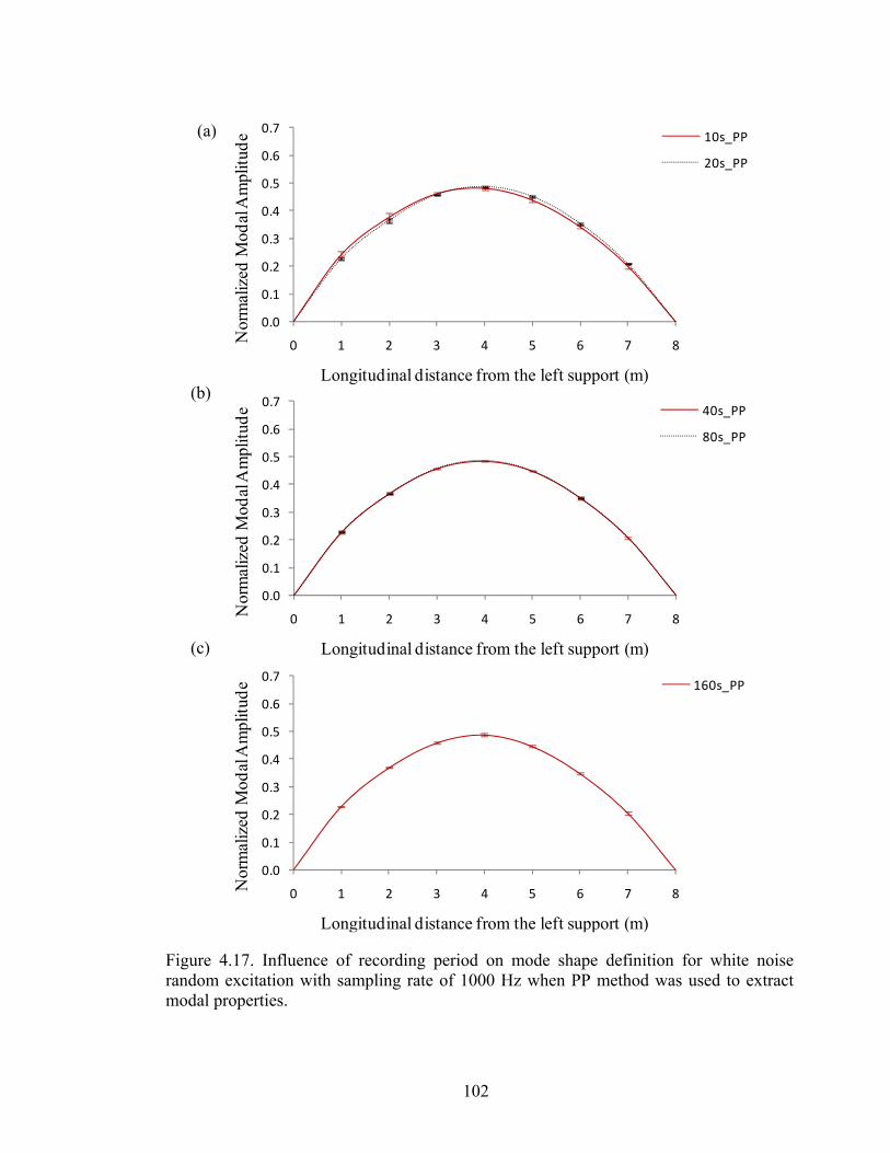
102
0.0
0.1
0.2
0.3
0.4
0.5
0.6
0.7
0 1 2 3 4 5 6 7 8Nor
mal
ized
Mod
al A
mpl
itud
e
Longitudinal distance from the left support (m)
160s_PP
0.0
0.1
0.2
0.3
0.4
0.5
0.6
0.7
0 1 2 3 4 5 6 7 8Nor
mal
ized
Mod
al A
mpl
itud
e
Longitudinal distance from the left support (m)
40s_PP
80s_PP
0.0
0.1
0.2
0.3
0.4
0.5
0.6
0.7
0 1 2 3 4 5 6 7 8Nor
mal
ized
Mod
al A
mpl
itud
e
Longitudinal distance from the left support (m)
10s_PP
20s_PP
Figure 4.17. Influence of recording period on mode shape definition for white noiserandom excitation with sampling rate of 1000 Hz when PP method was used to extractmodal properties.
(a)
(b)
(c)
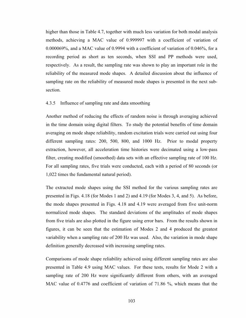
103
higher than those in Table 4.7, together with much less variation for both modal analysis
methods, achieving a MAC value of 0.999997 with a coefficient of variation of
0.000069%, and a MAC value of 0.9994 with a coefficient of variation of 0.046%, for a
recording period as short as ten seconds, when SSI and PP methods were used,
respectively. As a result, the sampling rate was shown to play an important role in the
reliability of the measured mode shapes. A detailed discussion about the influence of
sampling rate on the reliability of measured mode shapes is presented in the next sub-
section.
4.3.5 Influence of sampling rate and data smoothing
Another method of reducing the effects of random noise is through averaging achieved
in the time domain using digital filters. To study the potential benefits of time domain
averaging on mode shape reliability, random excitation trials were carried out using four
different sampling rates: 200, 500, 800, and 1000 Hz. Prior to modal property
extraction, however, all acceleration time histories were decimated using a low-pass
filter, creating modified (smoothed) data sets with an effective sampling rate of 100 Hz.
For all sampling rates, five trials were conducted, each with a period of 80 seconds (or
1,022 times the fundamental natural period).
The extracted mode shapes using the SSI method for the various sampling rates are
presented in Figs. 4.18 (for Modes 1 and 2) and 4.19 (for Modes 3, 4, and 5). As before,
the mode shapes presented in Figs. 4.18 and 4.19 were averaged from five unit-norm
normalized mode shapes. The standard deviations of the amplitudes of mode shapes
from five trials are also plotted in the figure using error bars. From the results shown in
figures, it can be seen that the estimation of Modes 2 and 4 produced the greatest
variability when a sampling rate of 200 Hz was used. Also, the variation in mode shape
definition generally decreased with increasing sampling rates.
Comparisons of mode shape reliability achieved using different sampling rates are also
presented in Table 4.9 using MAC values. For these tests, results for Mode 2 with a
sampling rate of 200 Hz were significantly different from others, with an averaged
MAC value of 0.4776 and coefficient of variation of 71.86 %, which means that the

104
mode shape estimation was highly unreliable. Actually, there were no stable poles
available for this mode in the stabilization plots using the SSI modal identification
method; in fact, this mode was inadvertently overlooked in previously published results
(Wang et al. 2008). From the results listed in Table 4.7, it can be seen that the reliability
of the fundamental mode shape continued to improve with increasing sampling rates up
to 1000 Hz. As the mode number increased, however, the benefits of the time domain
averaging made possible by higher sampling rates appeared to diminish until, for Mode
5, there is no apparent improvement in mode shape reliability associated with increased
sampling rates.
‐0.7
‐0.5
‐0.3
‐0.1
0.1
0.3
0.5
0.7
0 1 2 3 4 5 6 7 8
Nor
mal
ized
Mod
al A
mpl
itud
e
Longitudinal distance from the left support (m)
200 Hz
500 Hz
800 Hz
1000 Hz
‐0.7
‐0.5
‐0.3
‐0.1
0.1
0.3
0.5
0.7
0 1 2 3 4 5 6 7 8N
orm
aliz
ed M
odal
Am
plit
ude
Longitudinal distance from the left support (m)
200 Hz
500 Hz
800 Hz
1000 Hz
Figure 4.18. Influence of sampling rate on mode shape definition of: (a) Mode 1; (b)Mode 2 for white noise random excitation with recording period of 80 seconds, whenthe SSI method was used to extract modal properties.
(a)
(b)
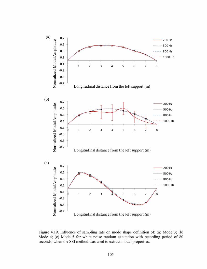
105
‐0.7
‐0.5
‐0.3
‐0.1
0.1
0.3
0.5
0.7
0 1 2 3 4 5 6 7 8
Nor
mal
ized
Mod
al A
mpl
itud
e
Longitudinal distance from the left support (m)
200 Hz
500 Hz
800 Hz
1000 Hz
‐0.7
‐0.5
‐0.3
‐0.1
0.1
0.3
0.5
0.7
0 1 2 3 4 5 6 7 8
Nor
mal
ized
Mod
al A
mpl
itud
e
Longitudinal distance from the left support (m)
200 Hz
500 Hz
800 Hz
1000 Hz
‐0.7
‐0.5
‐0.3
‐0.1
0.1
0.3
0.5
0.7
0 1 2 3 4 5 6 7 8
Nor
mal
ized
Mod
al A
mpl
itud
e
Longitudinal distance from the left support (m)
200 Hz
500 Hz
800 Hz
1000 Hz
Figure 4.19. Influence of sampling rate on mode shape definition of: (a) Mode 3; (b)Mode 4; (c) Mode 5 for white noise random excitation with recording period of 80seconds, when the SSI method was used to extract modal properties.
(a)
(b)
(c)

106
4.4 Influence of Normalization on Mode Shape Definition and Change in Mode
Shape Due to Damage
4.4.1 Overview
Although the shape of vibration modes (i.e., the ratio of modal amplitudes at different
measurement points) is determinate, the amplitude of mode shapes is indeterminate in
most cases, especially for dynamic tests of civil engineering structures, where the input
excitation forces are typically not quantified. As a result, it is necessary to normalize (or
scale) the mode shapes with respect to a common base in order to investigate the relative
changes in mode shapes caused by damage. There are many different ways to normalize
the mode shapes.
One normalization method commonly used in eigenvector analysis is to select one
element as a benchmark point (usually the element with maximum relative amplitude)
and scale it to a constant value (for example, unity); the remaining elements are then
Table 4.9. Influence of sampling rates and time domain averaging on mode shape reliability based on averaged MAC values from five repeated trials with white noise random excitation.
Sampling rate (Hz) Averaged MAC value
200 500 800 1000
Mode 1 Avg. 0.99640644 0.99996793 0.99999927 0.99999975
C.O.V. 0.42458% 0.00371% 0.00003% 0.00001%
Mode 2 Avg. 0.47760945 0.99773264 0.99995200 0.99998641
C.O.V. 71.85969% 0.26686% 0.00573% 0.00116%
Mode 3 Avg. 0.99816765 0.99976419 0.99995609 0.99993072
C.O.V. 0.13198% 0.01505% 0.00592% 0.00823%
Mode 4 Avg. 0.84915608 0.99981073 0.99992883 0.99903376
C.O.V. 29.69770% 0.01003% 0.01152% 0.11394%
Mode 5 Avg. 0.99945380 0.99842765 0.99864071 0.99547048
C.O.V. 0.03571% 0.11925% 0.08802% 0.72215% Avg. = Average; C.O.V. = Coefficient of variation.
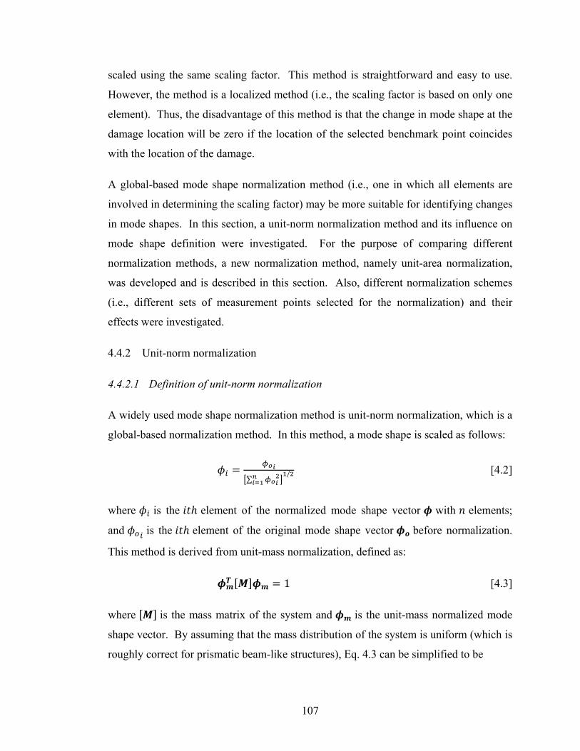
107
scaled using the same scaling factor. This method is straightforward and easy to use.
However, the method is a localized method (i.e., the scaling factor is based on only one
element). Thus, the disadvantage of this method is that the change in mode shape at the
damage location will be zero if the location of the selected benchmark point coincides
with the location of the damage.
A global-based mode shape normalization method (i.e., one in which all elements are
involved in determining the scaling factor) may be more suitable for identifying changes
in mode shapes. In this section, a unit-norm normalization method and its influence on
mode shape definition were investigated. For the purpose of comparing different
normalization methods, a new normalization method, namely unit-area normalization,
was developed and is described in this section. Also, different normalization schemes
(i.e., different sets of measurement points selected for the normalization) and their
effects were investigated.
4.4.2 Unit-norm normalization
4.4.2.1 Definition of unit-norm normalization
A widely used mode shape normalization method is unit-norm normalization, which is a
global-based normalization method. In this method, a mode shape is scaled as follows:
∑/ [4.2]
where is the element of the normalized mode shape vector with elements;
and is the element of the original mode shape vector before normalization.
This method is derived from unit-mass normalization, defined as:
1 [4.3]
where is the mass matrix of the system and is the unit-mass normalized mode
shape vector. By assuming that the mass distribution of the system is uniform (which is
roughly correct for prismatic beam-like structures), Eq. 4.3 can be simplified to be
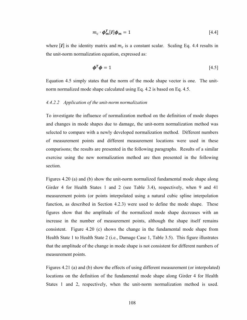
108
∙ 1 [4.4]
where is the identity matrix and is a constant scalar. Scaling Eq. 4.4 results in
the unit-norm normalization equation, expressed as:
1 [4.5]
Equation 4.5 simply states that the norm of the mode shape vector is one. The unit-
norm normalized mode shape calculated using Eq. 4.2 is based on Eq. 4.5.
4.4.2.2 Application of the unit-norm normalization
To investigate the influence of normalization method on the definition of mode shapes
and changes in mode shapes due to damage, the unit-norm normalization method was
selected to compare with a newly developed normalization method. Different numbers
of measurement points and different measurement locations were used in these
comparisons; the results are presented in the following paragraphs. Results of a similar
exercise using the new normalization method are then presented in the following
section.
Figures 4.20 (a) and (b) show the unit-norm normalized fundamental mode shape along
Girder 4 for Health States 1 and 2 (see Table 3.4), respectively, when 9 and 41
measurement points (or points interpolated using a natural cubic spline interpolation
function, as described in Section 4.2.3) were used to define the mode shape. These
figures show that the amplitude of the normalized mode shape decreases with an
increase in the number of measurement points, although the shape itself remains
consistent. Figure 4.20 (c) shows the change in the fundamental mode shape from
Health State 1 to Health State 2 (i.e., Damage Case 1, Table 3.5). This figure illustrates
that the amplitude of the change in mode shape is not consistent for different numbers of
measurement points.
Figures 4.21 (a) and (b) show the effects of using different measurement (or interpolated)
locations on the definition of the fundamental mode shape along Girder 4 for Health
States 1 and 2, respectively, when the unit-norm normalization method is used.

109
-0.008
-0.006
-0.004
-0.002
0.000
0.002
0.004
0.006
0.008
0 1 2 3 4 5 6 7 8Am
plitu
de
Longitudinal distance from the support (m)
9 points 41 points
0.00
0.10
0.20
0.30
0.40
0.50
0.60
0 1 2 3 4 5 6 7 8
Am
plitu
de
Longitudinal distance from the support (m)
9 points 41 points
0.00
0.10
0.20
0.30
0.40
0.50
0.60
0 1 2 3 4 5 6 7 8
Am
plitu
de
Longitudinal distance from the support (m)
9 points 41 points
Figure 4.20. Influence of unit-norm normalization on: (a) Mode 1 in Health State 1, (b)Mode 1 in Health State 2, and (c) Change in mode shape for Damage Case 1, when adifferent number of measurement points was used.
(a)
(b)
(c)

110
-0.008
-0.006
-0.004
-0.002
0.000
0.002
0.004
0.006
0.008
0 1 2 3 4 5 6 7 8Am
plitu
de
Longitudinal distance from the support (m)
9 points 9 points with different locations
0.00
0.10
0.20
0.30
0.40
0.50
0.60
0 1 2 3 4 5 6 7 8
Am
plitu
de
Longitudinal distance from the support (m)
9 points 9 points with different locations
0.00
0.10
0.20
0.30
0.40
0.50
0.60
0 1 2 3 4 5 6 7 8
Am
plitu
de
Longitudinal distance from the support (m)
9 points 9 points with different locations
Figure 4.21. Influence of unit-norm normalization on: (a) Mode 1 in Health State 1, (b)Mode 1 in Health State 2, and (c) Change in mode shape in Damage Case 1, whendifferent measurement locations were used.
(a)
(b)
(c)

111
Figure 4.21 (c) shows the influence of using different measurement locations on the
change in the fundamental mode shape due to Damage Case 1 when unit-norm
normalization was used. From these figures, it can be seen that both the amplitude of
the mode shape and the amplitude of the change in mode shape due to damage vary
when different measurement locations are used.
In summary, it can be concluded that both the amplitude of mode shapes and the
amplitude of changes in mode shapes due to damage depend on the number and
locations of measurement points selected, when the unit-norm normalization method is
adopted to normalize the mode shapes. Thus, the mode shape definition and change in
mode shape are not unique, which makes it inconvenient to analyze the results in a
statistical manner, since the statistical values depends on the number and locations of
measurement points selected. It is still possible to use unit-norm normalization to
calculate changes in mode shapes, and characterize the results in terms of statistical
distributions. However, statistical evaluations of unit-norm mode shapes are usually
based on the statistical values (for example, standard deviation and coefficient of
variation) of components of mode shapes (i.e., the statistical values of mode shape
amplitudes at certain measurement points) or their combinations (i.e., using the mode
shape amplitudes at multiple measurement points together), instead of the mode shapes
themselves, which usually have no clear physical meaning.
More importantly, it is not easy to determine whether or not damage is present only
from examining peaks in the plots of change in mode shape, even though peaks often
coincide with locations of damage and may also indicate the presence of damage. This
is because the peaks may be due to either damage or random variability in the
measurements, while the amplitude of mode shapes, as well as the changes in mode
shapes, decrease with an increasing number of measurement points. In other words, it is
not easy to claim the presence of damage by only checking the amplitude of changes in
mode shapes, no matter how big or small they are. The amplitudes of the changes in
mode shapes using unit-norm normalization are usually very small, with numbers of the
order of 10-5, 10-6, or 10-7, depending on the number of measurement (or interpolation)
points used and the severity of damage experienced. For example, the different numbers

112
of measurement (or interpolation) points used in this research included 19 strain gauge
points (five gauges along the first three girders, four gauges along the fourth girder), 28
accelerometer points (seven points along each girder line), 41 interpolated points for
both strain gauges and accelerometers, and an infinite number points expressed as a
continuous function for both sensors.
However, uncertainties inherent in the practical dynamic tests led to variability in the
measured mode shapes from separate data sets. Thus, there are some peaks present in
the plots of changes in mode shapes resulting from the comparison of those separate
data sets even when the condition of the structure has not changed during the tests. If
the mode shapes are normalized using unit-norm normalization, it is not easy to
determine whether these peaks are caused by random variability or other uncertainties
by observing the amplitude of changes, no matter how small the amplitudes are, because
amplitudes caused by some severe damage case could be small if the number of
measurement (or interpolation) points is large enough. On the other hand, it is not easy
to claim that there is damage present no matter how big the amplitude of change in
mode shape is.
As a result, it is necessary to identify a normalization method by which the normalized
mode shapes would be uniquely defined no matter how many measurement points are
used and where the sensors are located. Furthermore, it is necessary to look for a
statistically-based Level 1 damage indicator for the practical application of VBDD.
4.4.3 Unit-area normalization
4.4.3.1 Definition of the unit-area normalization
A global-based normalization method, referred to as the unit-area method, was
developed in this research, providing a unique definition of mode shape, in part, so that
the normalization process would depend to a lesser extent on the number and location of
measurement points used. This method was also well-suited for use as a Level 1
damage identification method. It should be acknowledged that a very similar

113
normalization method was found in the literature, but only after it had been
independently developed as part of this thesis work (Huth et al. 2005).
The method is defined as follows:
[4.6]
where is the element of the normalized mode shape vector with elements;
and represents the element of the original mode shape vector before
normalization. In addition, represents the area enclosed by the plot of the
absolute value of the mode shape, defined as:
| | [4.7]
where represents the interpolated mode shape function and corresponds to the
distance along the measurement line ( in this case, the girder lines). The mode shape
function was found by first fitting a natural cubic spline interpolation function to
the modal amplitudes at sensor locations along each girder, creating a piecewise cubic
polynomial that passed through all the measured amplitudes. The spline function
featured continuous first and second derivatives at measurement points, and zero
curvature at supports. The range of integration is expressed here from 0 to 1 because the
length of the measurement line is first scaled to be equal to one. For the case of multiple
measurement lines, the individual mode shapes for all measurement lines are strung end
to end to create a single mode shape vector for the entire structure, with the resulting
length adjusted to be equal to one (see Fig. 4.22). It should be acknowledged that other
schemes, including different interpolation and numerical integration methods, are also
acceptable to calculate the area enclosed by the mode shapes.
4.4.3.2 Application of unit-area normalization
To compare the different effects of the unit-norm and unit-area normalization methods
on the definition of mode shapes and changes in mode shapes due to damage, the unit-
area normalization method, given in Eq. 4.6, was adopted to normalize the same mode
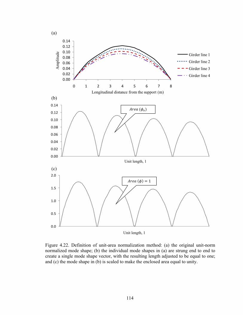
114
0.0
0.5
1.0
1.5
2.0
0.00
0.02
0.04
0.06
0.08
0.10
0.12
0.14
0.00
0.02
0.04
0.06
0.08
0.10
0.12
0.14
0 1 2 3 4 5 6 7 8
Am
plit
ude
Longitudinal distance from the support (m)
Girder line 1
Girder line 2
Girder line 3
Girder line 4
Figure 4.22. Definition of unit-area normalization method: (a) the original unit-normnormalized mode shape; (b) the individual mode shapes in (a) are strung end to end tocreate a single mode shape vector, with the resulting length adjusted to be equal to one;and (c) the mode shape in (b) is scaled to make the enclosed area equal to unity.
(a)
(b)
Unit length, 1
Unit length, 1
1
(c)

115
shapes used in Figs. 4.20 and 4.21, where different numbers of measurement points and
different measurement locations were considered. The resulting normalized mode
shapes and changes in mode shapes are presented in Figs. 4.23 and 4.24.
Figure 4.23 shows the influence of using different numbers of measurement (or
interpolation) points (9 and 41 points) on the mode shape definitions and the change in
mode shape for Damage Case 1, when unit-area normalization is used. It is evident that
unit-area normalization generated the same mode shape definition (Figs. 4.23 (a) and
(b)) and the same definition of the corresponding change in mode shape (Fig. 4.23 (c)),
when different numbers of measurement points were used.
Figures 4.24 (a) and (b) show the influence of using different measurement (or
interpolation) locations on the definition of the fundamental mode shape along Girder 4
for Health States 1 and 2, respectively, while Figure 4.24 (c) presents the effects on the
change in the fundamental mode shape due to Damage Case 1, when the unit-area
method was adopted to normalize the mode shapes. It can be seen that the mode shape
definition and the corresponding changes in mode shapes were consistent and coincided
with each other no matter where the sensors were located.
In summary, it can be concluded that the unit-area normalization process produced a
more consistent mode shape definition and corresponding change in mode shape than
the widely used unit-norm method, when considering different numbers and locations of
measurement points. As a result, the unit-area normalization method was adopted in
this research, in part, so that the normalization process would be less sensitive to the
number and location of sensors used. More importantly, the feature of a unique mode
shape definition makes it convenient to analyze the change in mode shape for damage
detection in a statistical manner. Based on the unit-area method, a scalar damage
indicator was developed in Chapter 5 and the sensitivities of the various test procedures
were investigated in Chapter 6.

116
-0.02
-0.01
0.00
0.01
0.02
0.03
0 1 2 3 4 5 6 7 8
Am
plitu
de
Longitudinal distance from the support (m)
9 points 41 points
0.000.200.400.600.801.001.201.401.601.80
0 1 2 3 4 5 6 7 8
Am
plitu
de
Longitudinal distance from the support (m)
9 points 41 points
0.000.200.400.600.801.001.201.401.601.80
0 1 2 3 4 5 6 7 8
Am
plitu
de
Longitudinal distance from the support (m)
9 points 41 points
Figure 4.23. Influence of unit-area normalization on: (a) Mode 1 in Health State 1, (b)Mode 1 in Health State 2, and (c) Change in mode shape for Damage Case 1, whendifferent numbers of measurement points were used.
(a)
(b)
(c)
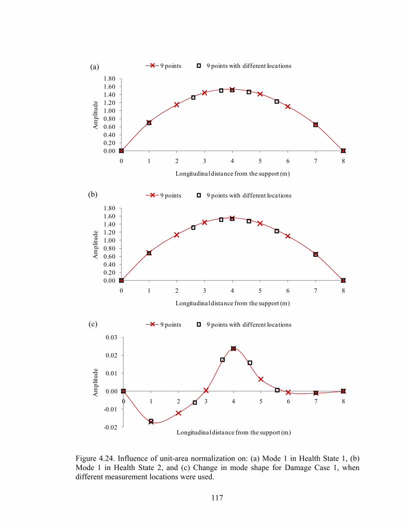
117
-0.02
-0.01
0.00
0.01
0.02
0.03
0 1 2 3 4 5 6 7 8
Am
plitu
de
Longitudinal distance from the support (m)
9 points 9 points with different locations
0.000.200.400.600.801.001.201.401.601.80
0 1 2 3 4 5 6 7 8
Am
plitu
de
Longitudinal distance from the support (m)
9 points 9 points with different locations
0.000.200.400.600.801.001.201.401.601.80
0 1 2 3 4 5 6 7 8
Am
plitu
de
Longitudinal distance from the support (m)
9 points 9 points with different locations
Figure 4.24. Influence of unit-area normalization on: (a) Mode 1 in Health State 1, (b)Mode 1 in Health State 2, and (c) Change in mode shape for Damage Case 1, whendifferent measurement locations were used.
(a)
(b)
(c)
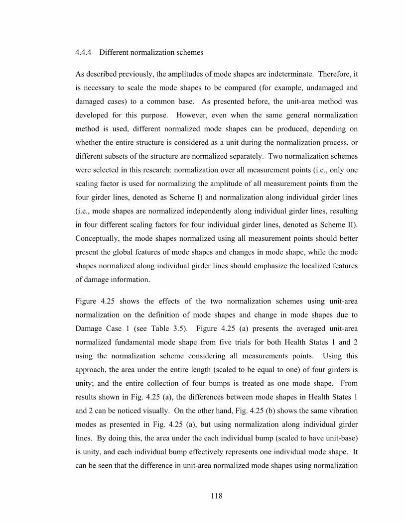
118
4.4.4 Different normalization schemes
As described previously, the amplitudes of mode shapes are indeterminate. Therefore, it
is necessary to scale the mode shapes to be compared (for example, undamaged and
damaged cases) to a common base. As presented before, the unit-area method was
developed for this purpose. However, even when the same general normalization
method is used, different normalized mode shapes can be produced, depending on
whether the entire structure is considered as a unit during the normalization process, or
different subsets of the structure are normalized separately. Two normalization schemes
were selected in this research: normalization over all measurement points (i.e., only one
scaling factor is used for normalizing the amplitude of all measurement points from the
four girder lines, denoted as Scheme I) and normalization along individual girder lines
(i.e., mode shapes are normalized independently along individual girder lines, resulting
in four different scaling factors for four individual girder lines, denoted as Scheme II).
Conceptually, the mode shapes normalized using all measurement points should better
present the global features of mode shapes and changes in mode shape, while the mode
shapes normalized along individual girder lines should emphasize the localized features
of damage information.
Figure 4.25 shows the effects of the two normalization schemes using unit-area
normalization on the definition of mode shapes and change in mode shapes due to
Damage Case 1 (see Table 3.5). Figure 4.25 (a) presents the averaged unit-area
normalized fundamental mode shape from five trials for both Health States 1 and 2
using the normalization scheme considering all measurements points. Using this
approach, the area under the entire length (scaled to be equal to one) of four girders is
unity; and the entire collection of four bumps is treated as one mode shape. From
results shown in Fig. 4.25 (a), the differences between mode shapes in Health States 1
and 2 can be noticed visually. On the other hand, Fig. 4.25 (b) shows the same vibration
modes as presented in Fig. 4.25 (a), but using normalization along individual girder
lines. By doing this, the area under the each individual bump (scaled to have unit-base)
is unity, and each individual bump effectively represents one individual mode shape. It
can be seen that the difference in unit-area normalized mode shapes using normalization

119
Scheme II shown in Fig. 4.25(b) between Health States 1 and 2 is not noticeable
visually, although the difference may still be significant.
Figures 4.25 (c) and (d) represent the changes in fundamental mode shape due to
Damage Case 1 (a comparison of Health States 1 and 2) using the unit-area
normalization over all measurements points and along individual girder lines,
respectively. It can be concluded that the normalization over all measurement points
reflects the global changes in mode shape, which may locate the possible damage in
both the longitudinal and transverse directions. For example, in Fig. 4.25 (c), the
maximum change in mode shape is located at the mid-span of Girder 4, coinciding with
the damage location for Damage Case 1. It can be also concluded that normalization
along individual girder lines can magnify the changes locally, narrowing the range of
possible damage locations and thereby benefitting the damage localization in another
way. As a result, in practice, the two different normalization schemes should be used
simultaneously to reflect both global and magnified local information regarding changes
in mode shapes. The application of the two normalization schemes is presented in
Chapter 6.
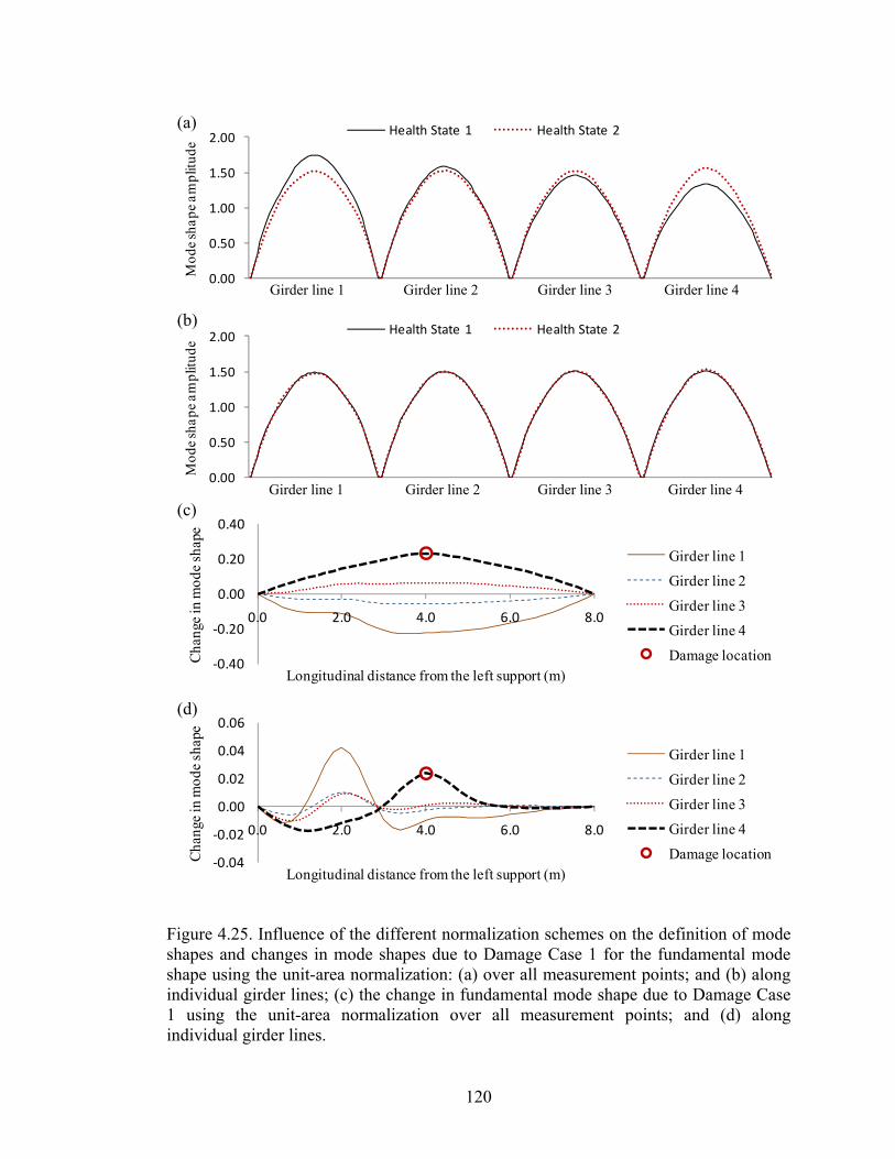
120
‐0.04
‐0.02
0.00
0.02
0.04
0.06
0.0 2.0 4.0 6.0 8.0
Cha
nge
in m
ode
shap
e
Longitudinal distance from the left support (m)
Girder line 1
Girder line 2
Girder line 3
Girder line 4
Damage location
‐0.40
‐0.20
0.00
0.20
0.40
0.0 2.0 4.0 6.0 8.0
Cha
nge
in m
ode
shap
e
Longitudinal distance from the left support (m)
Girder line 1
Girder line 2
Girder line 3
Girder line 4
Damage location
0.00
0.50
1.00
1.50
2.00
Mod
e sh
ape
ampl
itude
Health State 1 Health State 2
0.00
0.50
1.00
1.50
2.00
Mod
e sh
ape
ampl
itude
Health State 1 Health State 2
Figure 4.25. Influence of the different normalization schemes on the definition of modeshapes and changes in mode shapes due to Damage Case 1 for the fundamental modeshape using the unit-area normalization: (a) over all measurement points; and (b) alongindividual girder lines; (c) the change in fundamental mode shape due to Damage Case1 using the unit-area normalization over all measurement points; and (d) alongindividual girder lines.
Girder line 1 Girder line 2 Girder line 3 Girder line 4
Girder line 1 Girder line 2 Girder line 3 Girder line 4
(a)
(b)
(c)
(d)

121
CHAPTER 5. LEVEL 1 VBDD INDICATOR
DEVELOPED: THE AREA OF MODE SHAPE CHANGE
5.1 Overview
Numerous VBDD methods which are related in some manner to changes in modal
parameters (notably natural frequencies, damping, and mode shapes) have been
proposed as a potential techniques for structural health monitoring (Wolf and
Richardson 1989, Wegner et al. 2004). Although there have been some successful
applications of the proposed VBDD methods, there are still great challenges associated
with practically applying the methods to complicated structural systems like bridges.
Changes in natural frequencies have proven not to be sensitive enough to detect small
scale damage in practical situations, especially considering the experimental
uncertainties associated with temperature and other environmental conditions (Doebling
et at. 1996). The damage detection methods based on changes in damping have been
found to be unreliable and also not sensitive to small scale damage (Casas and Aparicio
1994, Salawu and Williams 1995, and Farrar and Jauregui 1998a). On the other hand,
methods based on mode shapes and their derivatives have been found to be effective
damage indicators (Pandey et al. 1991, Fox 1992, Srinivasan and Kot 1992, Salawu and
Williams 1994, and Zhang and Aktan 1995 and 1998). However, most of the proposed
methods based on mode shapes have not really addressed the problem of identifying the
presence of damage considering statistically reliable levels of confidence, which is
considered to be the most appropriate approach for practical problems with high levels
of uncertainty. This limitation may be partially due to the fact that the definition of a
mode shape is not unique, which makes the investigation of mode shapes in a statistical
manner difficult.
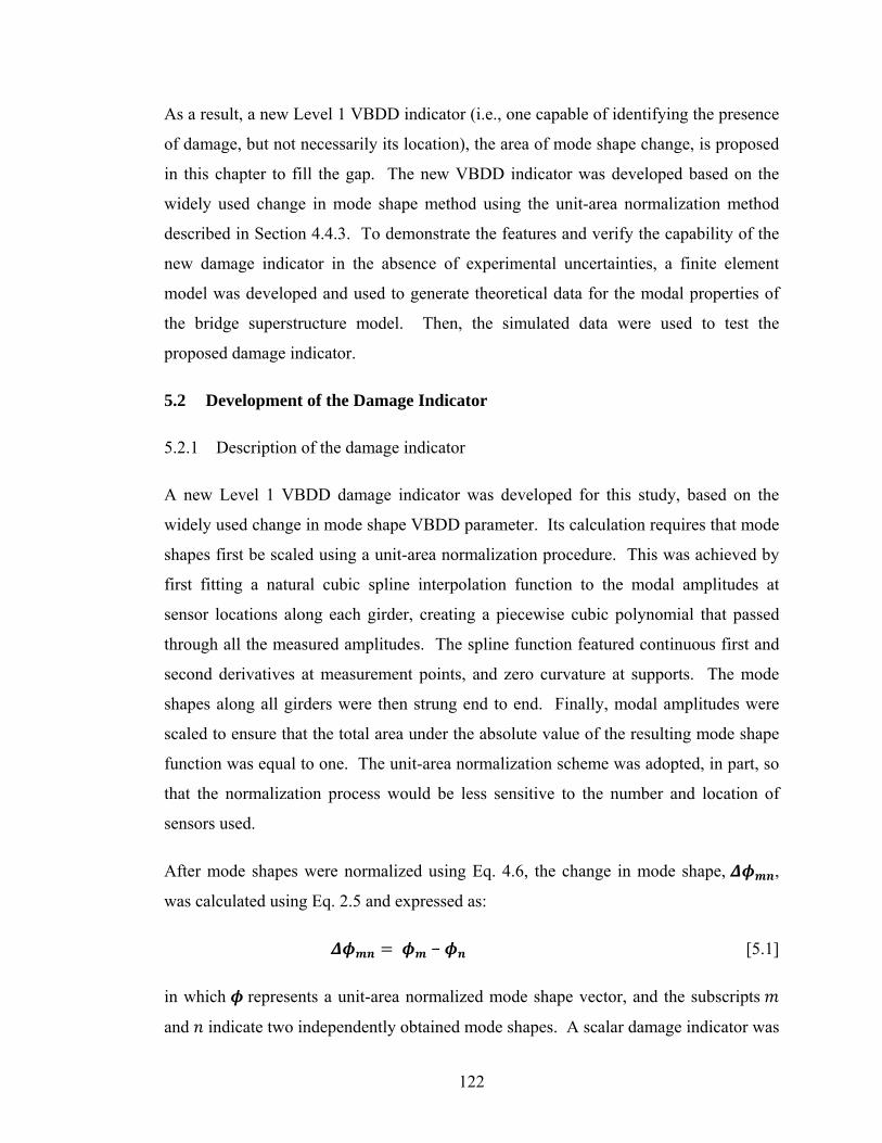
122
As a result, a new Level 1 VBDD indicator (i.e., one capable of identifying the presence
of damage, but not necessarily its location), the area of mode shape change, is proposed
in this chapter to fill the gap. The new VBDD indicator was developed based on the
widely used change in mode shape method using the unit-area normalization method
described in Section 4.4.3. To demonstrate the features and verify the capability of the
new damage indicator in the absence of experimental uncertainties, a finite element
model was developed and used to generate theoretical data for the modal properties of
the bridge superstructure model. Then, the simulated data were used to test the
proposed damage indicator.
5.2 Development of the Damage Indicator
5.2.1 Description of the damage indicator
A new Level 1 VBDD damage indicator was developed for this study, based on the
widely used change in mode shape VBDD parameter. Its calculation requires that mode
shapes first be scaled using a unit-area normalization procedure. This was achieved by
first fitting a natural cubic spline interpolation function to the modal amplitudes at
sensor locations along each girder, creating a piecewise cubic polynomial that passed
through all the measured amplitudes. The spline function featured continuous first and
second derivatives at measurement points, and zero curvature at supports. The mode
shapes along all girders were then strung end to end. Finally, modal amplitudes were
scaled to ensure that the total area under the absolute value of the resulting mode shape
function was equal to one. The unit-area normalization scheme was adopted, in part, so
that the normalization process would be less sensitive to the number and location of
sensors used.
After mode shapes were normalized using Eq. 4.6, the change in mode shape, ,
was calculated using Eq. 2.5 and expressed as:
− [5.1]
in which represents a unit-area normalized mode shape vector, and the subscripts
and indicate two independently obtained mode shapes. A scalar damage indicator was

123
derived from the change in mode shape vector by calculating the absolute value of the
area under :
Δ |Δ | [5.2]
where corresponds to the distance along girders (with all four girders included).
While the areas under the two mode shape vectors, and , are identical by virtue
of the unit-area normalization procedure, the distribution of the area over the length of
the structure will differ, producing a non-zero area under the difference function. The
area of the mode shape change, Δ , can therefore be used as an indicator of the presence
of damage. The Δ parameter can be expected to increase as damage becomes more
severe, leading to an increase in the likelihood of detecting the damage.
5.2.2 Features of the new damage indicator
One of the primary features of the new area of mode shape change damage indicator is
that its variability can be defined in terms of statistical parameters such that the presence
of damage can be established by comparison with certain levels of confidence. Specific
features of the indicator are as follows:
It was developed based on the widely used change in mode shape method;
The mode shapes used for a comparison must first be scaled to a common basis
using unit-area normalization;
The values calculated by the indicator are well-suited to statistical analysis; and
It is relatively insensitive to the number and location of measurement points
used.
5.2.3 Differences between the area of mode shape change and “mode shape area index”
It should be acknowledged that a VBDD damage indicator, called mode shape area
index, very similar to the one developed as part of this thesis work was found in the
literature during the later stages of preparation of this thesis (Huth et al. 2005).
However, the work presented in this thesis was developed independently and was
124
defined and applied in a different manner on a different application. Some differences
between two damage indicators are as follows:
They are somewhat different at the normalization stage. For the area of mode
shape indicator developed in this study, the length of the measurement line is
first scaled to be equal to one before calculating the area enclosed by mode
shapes. For the case of multiple measurement lines, the individual mode shapes
for all measurement lines are strung end to end to create a single mode shape
vector for the entire structure, with the resulting length adjusted to be equal to
one (see Section 4.4.3). This normalization method results in a unique mode
shape definition no matter how many measurement lines are used and what the
span of a particular bridge is; this makes the method convenient to apply the
change in mode shape for damage detection in statistical manner. There is no
such process for the “mode shape area index” indicator.
The “mode shape area index” indicator was evaluated by calculating ratios of the
area of one health state to that of the reference state. Since the longitudinal axis
of the tested bridge was divided into several parts, different ratios were
calculated for different parts of the bridge. These ratios are either larger or
smaller than one if the condition of the bridge changed. However, in the area of
mode shape indicator, the resulting area under the plot of the difference between
two independently measured mode shapes was calculated to evaluate the
changes of health conditions. In this way, only one value (from 0 to 1) was
generated for the mode shapes compared (see Section 5.2.1).
The application of the area of mode shape change indicator using a statistical
approach is believed to be original, and was not found in Huth et al. (2005).
5.3 Verification of the Damage Indicator Using Numerical Data
5.3.1 Description of the finite element model
Figure 5.1 shows the finite element model used for this verification, which was created
using the commercial finite element analysis software ANSYS (2005) based on the
experimental bridge model. The model featured four steel girders supporting a
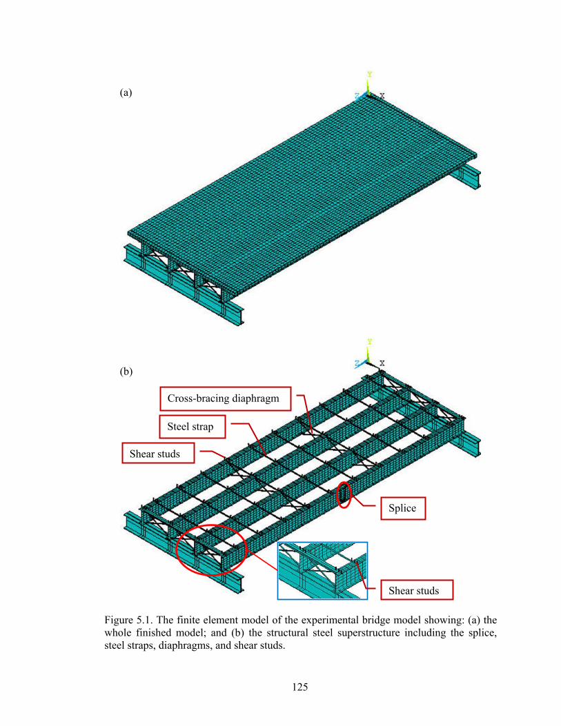
125
Figure 5.1. The finite element model of the experimental bridge model showing: (a) thewhole finished model; and (b) the structural steel superstructure including the splice,steel straps, diaphragms, and shear studs.
(a)
(b)
Splice
Shear studs
Cross-bracing diaphragm
Steel strap
Shear studs
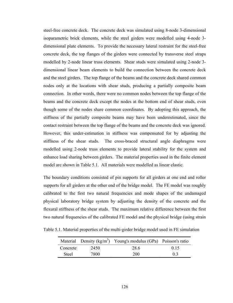
126
steel-free concrete deck. The concrete deck was simulated using 8-node 3-dimensional
isoparametric brick elements, while the steel girders were modelled using 4-node 3-
dimensional plate elements. To provide the necessary lateral restraint for the steel-free
concrete deck, the top flanges of the girders were connected by transverse steel straps
modelled by 2-node linear truss elements. Shear studs were simulated using 2-node 3-
dimensional linear beam elements to build the connection between the concrete deck
and the steel girders. The top flange of the beams and the concrete deck shared common
nodes only at the locations with shear studs, producing a partially composite beam
connection. In other words, there were no common nodes between the top flange of the
beams and the concrete deck except the nodes at the bottom end of shear studs, even
though some of the nodes share common coordinates. By adopting this approach, the
stiffness of the partially composite beams may have been underestimated, since the
contact restraint between the top flange of the beams and the concrete deck was ignored.
However, this under-estimation in stiffness was compensated for by adjusting the
stiffness of the shear studs. The cross-braced structural angle diaphragms were
modelled using 2-node truss elements to provide lateral stability for the system and
enhance load sharing between girders. The material properties used in the finite element
model are shown in Table 5.1. All materials were modelled as linear elastic.
The boundary conditions consisted of pin supports for all girders at one end and roller
supports for all girders at the other end of the bridge model. The FE model was roughly
calibrated to the first two natural frequencies and mode shapes of the undamaged
physical laboratory bridge system by adjusting the density of the concrete and the
flexural stiffness of the shear studs. The maximum relative difference between the first
two natural frequencies of the calibrated FE model and the physical bridge (using strain
Table 5.1. Material properties of the multi-girder bridge model used in FE simulation
Material Density (kg/m3) Young's modulus (GPa) Poisson's ratio
Concrete 2450 28.6 0.15 Steel 7800 200 0.3

127
gauge data) was 2.73%. It should be acknowledged that the FE model could have been
calibrated to a better representation of the physical system if more parameters and
adjustments had been made. However, the calibrated model described was considered
to be sufficiently accurate to fulfill the purpose of this verification. The FE model was
treated as an independent model to generate some theoretical data of modal properties in
the absence of experimental uncertainties. No comparison between the FE model and
the physical model were made.
5.3.2 Description of simulated health states and damage cases
Once the FE model had been calibrated and the baseline dynamic properties of the
model had been established, two categories of damage states were introduced into the
simulated model, consisting of damage to the steel girders and damage to the concrete
deck. Altogether, twelve different health states were investigated in this simulation, as
described in the following paragraphs.
For damage category 1 (Fig. 5.2), simulated damage states were incrementally
introduced into the steel Girder 4 at mid-span. Figure 5.2 (a) shows the intact condition
of the splice at mid-span of Girder 4 before any damage was introduced; this was
considered as simulated Health State 1. Figure 5.2 (b) represents the damage case in
which the bottom plate was removed from the splice. This was similar to Damage Case
1 for the physical model, as shown in Table 3.5; it is referred to here as simulated Health
State 2 or simulated Damage Case 1 since Health State 1 was treated as the baseline
condition. Figure 5.2 (c) and d show the incrementally increasing level of damage
induced at the splice by eliminating some plate elements in the web splice connection;
these are described as simulated Damage Cases 10 and 11, respectively. The
incrementally increasing damage conditions shown in Figs. 5.2 (b), (c), and (d)
produced reductions in the vertical flexural stiffness at that location of 7.76%, 9.17%,
and 19.02%, respectively (see Table 5.2). The flexural stiffness for each health state
was calculated by applying a concentrated vertical force at the splice location and
observing the corresponding displacement at the same location. For example, a
localized flexural stiffness of 88 kN/mm was calculated for Health State 1 by applying a

128
vertical load of 1 kN and using the corresponding vertical displacement of 0.0114 mm at
that location.
For damage category 2 (Fig. 5.3), small square blocks of concrete, 100 X 100 mm in
plan and 25 mm deep, were incrementally removed from the top surface of the concrete
deck by eliminating one element at a time at a location near mid-span of Girders 3 and
4. Figure 5.3 shows Health States 3 to 10, with one to eight elements removed from the
surface of the simulated concrete deck, while Fig. 5.4 shows the general locations of the
removed elements. It should be noted that the previous damage (i.e., the damage case in
Health State 2, for which the bottom plate was removed from the splice) was not
repaired for the Health States 3 to 10. Thus Health State 2, instead of Health State 1,
was treated as the baseline condition for Damage Cases 2 to 9, as shown in Table 5.2.
Figure 5.2. The simulated damage states incrementally introduced to steel Girder 4 atthe splice connection: (a) Health State 1 (the intact condition), (b) Health State 2 (orDamage Case 1), (c) Health State 11 (or Damage Case 10), and (d) Health State 12 (orDamage Case 11).
(a) (b)
(c) (d)

129
These damage states produced reductions in the vertical flexural stiffness at the mid-
span of Girder 4 of 0.05% to 0.30 %, following a roughly linear relationship (see Table
5.2).
5.3.3 Results and discussion
5.3.3.1 Simulated model properties
The lowest five vibration modes of the FE model for various health states were
extracted using a modal analysis method, the Block Lanczos eigenvalue extraction
method, available in the finite element software ANSYS. This method is suitable for
large symmetric eigenvalue problems. Typically, the Block Lanczos method is
applicable to the type of problems solved using the Subspace eigenvalue method,
however, at a faster convergence rate. A comparison of the extracted natural
frequencies in various health states is presented in Table 5.3. Generally, the first two
natural frequencies decreased with increasing damage conditions. For damage category
1, the first natural frequency decreased by a maximum of 2.44 %, while the second
natural frequency decreased by 4.82 % (Health State 12). However, in Damage
Category 2, including Health States 3 through 10, the changes in natural frequencies
Table 5.2. Comparison of the flexural stiffness of the FE model for different health states extracted from the finite element model
Damage Case
Undamaged State
Damaged State
Type of damage
Relative change in vertical flexural stiffness
Case 1 State 1 State 2 To steel girder splice 7.76% Case 2 State 2 State 3 To concrete deck 0.05% Case 3 State 2 State 4 To concrete deck 0.09% Case 4 State 2 State 5 To concrete deck 0.12% Case 5 State 2 State 6 To concrete deck 0.15% Case 6 State 2 State 7 To concrete deck 0.21% Case 7 State 2 State 8 To concrete deck 0.24% Case 8 State 2 State 9 To concrete deck 0.26% Case 9 State 2 State 10 To concrete deck 0.30% Case 10 State 1 State 11 To steel girder splice 9.17% Case 11 State 1 State 12 To steel girder splice 19.02%
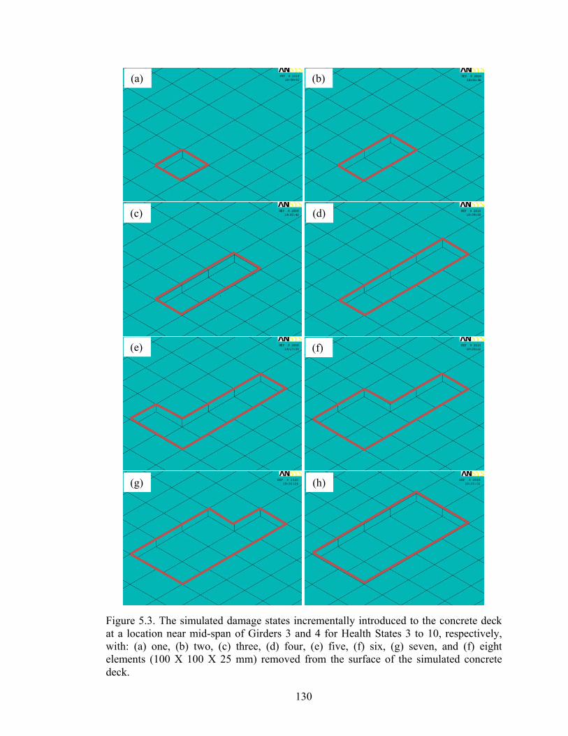
130
Figure 5.3. The simulated damage states incrementally introduced to the concrete deckat a location near mid-span of Girders 3 and 4 for Health States 3 to 10, respectively,with: (a) one, (b) two, (c) three, (d) four, (e) five, (f) six, (g) seven, and (f) eightelements (100 X 100 X 25 mm) removed from the surface of the simulated concretedeck.
(a) (b)
(c) (d)
(e) (f)
(g) (h)

131
Figure 5.4. The finite element model of the experimental bridge model: (a) the wholemeshed model; and (b) the physical model (before meshing), showing dimensions inmm; with an inset showing the order of the removed elements in Health States 3 to 10.
(a)
(b)
State 3
45
78
6910
4000
4000
Girder 3
Girder 4
450 450

132
were very small for all cases and were unnoticeable in some cases, with maximum
changes of 0.02%, considering all modes and all damage cases. This implies that
change in natural frequencies may not be a sensitive damage indicator for such small
scale damage cases.
The lowest five vibration mode shapes extracted for Health State 1 are presented in Fig.
5.5. The mode shapes are similar to those of the physical model (see Figs. 4.8, 4.9, and
4.10) except for Mode 5. Mode 1 is an unsymmetrical flexural mode shape; the
asymmetry is likely due to the presence of the over-designed splice connection on
Girder 4. Mode 2 is a torsional mode shape, while Mode 3 and Mode 4 exhibit
combined flexural and torsional behaviour. Mode 5 also presents a combination of
flexural and torsional behaviour, which is different from the physical model case, where
Mode 5 was the second flexural mode shape. No further calibration or investigation was
conducted regarding this difference.
Table 5.3. Comparison of simulated natural frequencies in different health states extracted from the finite element model
Mode The simulated natural frequencies (Hz)
State 1 State 2 State 3 State 4 State 5 State 6 1 13.119 13.049 13.049 13.050 13.050 13.051 2 14.298 13.977 13.978 13.979 13.979 13.980 3 29.408 29.294 29.294 29.295 29.295 29.295 4 32.242 32.175 32.176 32.176 32.177 32.177 5 36.148 32.999 32.999 32.999 32.998 32.998
Mode The simulated natural frequencies (Hz)
State 7 State 8 State 9 State 10 State 11 State 12 1 13.050 13.051 13.051 13.051 13.031 12.799 2 13.980 13.981 13.981 13.982 13.926 13.609 3 29.295 29.296 29.296 29.296 29.318 29.332 4 32.178 32.179 32.179 32.180 32.176 32.111 5 32.998 32.997 32.997 32.997 33.426 33.684

133
(a) (b)
(c) (d)
(e)
Figure 5.5. The lowest five vibration mode shapes for Health State 1 (the undamagedcondition) extracted from the finite element model: (a) Mode 1, (b) Mode 2, (c) Mode3, (d) Mode 4, and (e) Mode 5.
Girder 4 with splice

134
5.3.3.2 Change in modal properties due to damage
To calculate the area of mode shape change described in Eq. 5.2, the mode shapes to be
compared had to be normalized to a common basis using the unit-area normalization
method. Figures 5.6 and 5.7 give examples of the normalized mode shapes of the FE
model using the two different normalization schemes described in Section 4.4.4. Figure
5.6 presents the unit-area normalized first mode shape using the normalization scheme
0.0
0.5
1.0
1.5
2.0
2.5
0 1 2 3 4 5 6 7 8
Am
plitu
de
Longitudinal distance from the support (m)
Girder line 1 Girder line 2
Girder line 3 Girder line 4
0.0
0.5
1.0
1.5
2.0
2.5
0 1 2 3 4 5 6 7 8
Am
plitu
de
Longitudinal distance from the support (m)
Girder line 1 Girder line 2
Girder line 3 Girder line 4
Figure 5.6. The normalized mode shape of Mode 1 using the normalization scheme overall measurement points for: (a) simulated Health State 1 and (b) simulated Health State2.
(a)
(b)

135
over all measurement points (or selected nodes) for Health States 1 and 2, where the
global features of the mode shape can be noticed; in other words, the different girders
had different vibration amplitudes while the scaling ratio between girders remained
constant. Comparing Figs. 5.6(a) and (b), the difference in the distribution of modal
amplitudes due to damage can be visually noticed. Figures 5.7(a) and (b) show the unit-
area normalized first mode shape using the normalization scheme along individual
girder lines for simulated Health States 1 and 2, respectively. In this case, no
0.0
0.5
1.0
1.5
2.0
0 1 2 3 4 5 6 7 8
Am
plitu
de
Longitudinal distance from the support (m)
Girder line 1 Girder line 2
Girder line 3 Girder line 4
0.0
0.5
1.0
1.5
2.0
0 1 2 3 4 5 6 7 8
Am
plitu
de
Longitudinal distance from the support (m)
Girder line 1 Girder line 2
Girder line 3 Girder line 4
Figure 5.7. The normalized mode shape of Mode 1 using the normalization schemealong individual girder lines for: (a) simulated Health State 1 and (b) simulated HealthState 2.
(a)
(b)
136
pronounced differences can be noticed between mode shapes along different girder
lines.
After the mode shapes were normalized using unit-area normalization, Eq. 5.2 was used
to calculate the change in the mode shapes investigated. Using the same mode shapes
presented in Figs. 5.6 and 5.7, the change in mode shape due to the simulated damage
(Damage Case 1) is presented in Fig. 5.8, where Fig. 5.8(a) corresponds to
normalization over all measurement points and Fig. 5.8(b) corresponds to normalization
along the individual girder lines. Figure 5.8(a) shows global changes in mode shapes
due to the simulated Damage Case 1, featuring relatively large changes in modal
amplitudes for all girders. The maximum modal amplitude change (or increase due to
the presence of the simulated damage) occurred at the mid-span of Girder 4, with a
value of 0.324, which was 33.2 % of the mode shape amplitude at that location (0.977),
for this normalization scheme at the same location (see Fig. 5.6(a)). On the other hand,
Fig. 5.8(b) shows maximized local changes in mode shapes due to the same simulated
damage case, featuring relatively small, but localized, mode shape changes for all
girders. The maximum amplitude increase shown in Fig. 5.8(b) also occurred at the
mid-span of Girder 4, but with a much smaller value of 0.022, or 1.4 % of the mode
shape amplitude at the same location (see Fig. 5.7(a)). However, the shapes in Fig.
5.8(b) feature a much more prominent peak along Girder Line 4 than those shown in
Fig. 5.8(a). The ranges with positive amplitudes (i.e., indicating mode shape amplitude
increases due to damage) shown in Fig. 5.8(b) are much narrower (or more localized)
than those shown in Fig. 5.8(a); for example, for Girder Line 4, the range with positive
amplitudes in plots is from 2.8 to 5.2 m (longitudinal distance from the left support) in
Fig. 5.8(b), while in Fig. 5.8(a) the range is from 0 to 8.0 m.
Both normalization schemes were selected for further application to take advantage of
the combination of their benefits, reflecting both global changes (with relatively larger
amplitudes and perhaps less sensitivity to potential noise), which may be good for
determining the presence of damage globally, and maximized local changes in mode
shapes due to the damage, which may be useful to narrow the localized position of
damage. In this manner, the changes in mode shape for various simulated damage cases

137
were calculated, which was required for the calculation of the area of mode shape
change described in the next section.
5.3.3.3 The area of mode shape change due to simulated damage cases
To demonstrate the features and to verify the capabilities of the new damage indicator to
detect the presence of damage, the FE model described above was used to generate the
-0.015
-0.010
-0.005
0.000
0.005
0.010
0.015
0.020
0.025
0 1 2 3 4 5 6 7 8
Am
plit
ude
Longitudinal distance from the support (m)
Girder line 1 Girder line 2 Girder line 3
Girder line 4 Damage location
-0.40
-0.30
-0.20
-0.10
0.00
0.10
0.20
0.30
0.40
0 1 2 3 4 5 6 7 8Am
plitu
de
Longitudinal distance from the support (m)
Girder line 1 Girder line 2 Girder line 3
Girder line 4 Damage location
Figure 5.8. Change in mode shape due to the simulated Damage Case 1 using thenormalization schemes: (a) over all measurement points and (b) along the individualgirder lines.
(a)
(b)
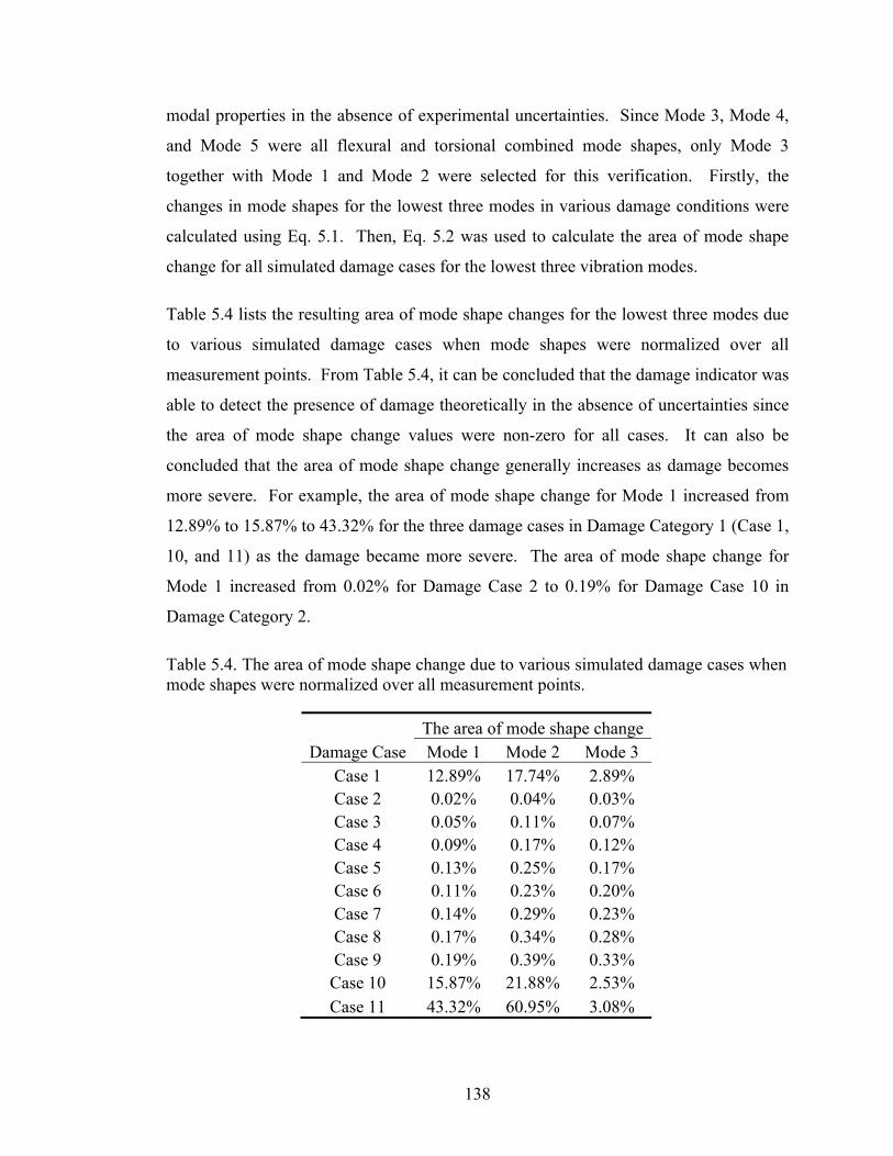
138
modal properties in the absence of experimental uncertainties. Since Mode 3, Mode 4,
and Mode 5 were all flexural and torsional combined mode shapes, only Mode 3
together with Mode 1 and Mode 2 were selected for this verification. Firstly, the
changes in mode shapes for the lowest three modes in various damage conditions were
calculated using Eq. 5.1. Then, Eq. 5.2 was used to calculate the area of mode shape
change for all simulated damage cases for the lowest three vibration modes.
Table 5.4 lists the resulting area of mode shape changes for the lowest three modes due
to various simulated damage cases when mode shapes were normalized over all
measurement points. From Table 5.4, it can be concluded that the damage indicator was
able to detect the presence of damage theoretically in the absence of uncertainties since
the area of mode shape change values were non-zero for all cases. It can also be
concluded that the area of mode shape change generally increases as damage becomes
more severe. For example, the area of mode shape change for Mode 1 increased from
12.89% to 15.87% to 43.32% for the three damage cases in Damage Category 1 (Case 1,
10, and 11) as the damage became more severe. The area of mode shape change for
Mode 1 increased from 0.02% for Damage Case 2 to 0.19% for Damage Case 10 in
Damage Category 2.
Table 5.4. The area of mode shape change due to various simulated damage cases when mode shapes were normalized over all measurement points.
The area of mode shape change Damage Case Mode 1 Mode 2 Mode 3
Case 1 12.89% 17.74% 2.89% Case 2 0.02% 0.04% 0.03% Case 3 0.05% 0.11% 0.07% Case 4 0.09% 0.17% 0.12% Case 5 0.13% 0.25% 0.17% Case 6 0.11% 0.23% 0.20% Case 7 0.14% 0.29% 0.23% Case 8 0.17% 0.34% 0.28% Case 9 0.19% 0.39% 0.33% Case 10 15.87% 21.88% 2.53% Case 11 43.32% 60.95% 3.08%
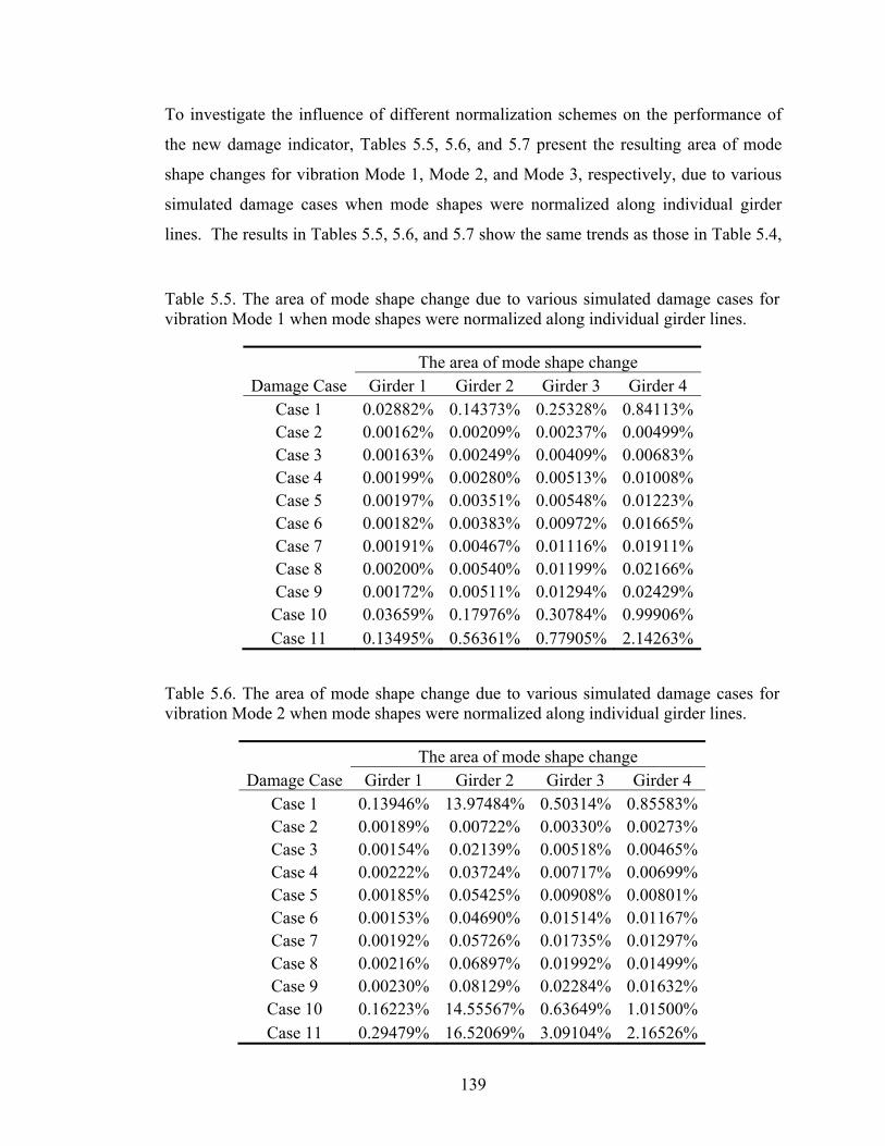
139
To investigate the influence of different normalization schemes on the performance of
the new damage indicator, Tables 5.5, 5.6, and 5.7 present the resulting area of mode
shape changes for vibration Mode 1, Mode 2, and Mode 3, respectively, due to various
simulated damage cases when mode shapes were normalized along individual girder
lines. The results in Tables 5.5, 5.6, and 5.7 show the same trends as those in Table 5.4,
Table 5.6. The area of mode shape change due to various simulated damage cases for vibration Mode 2 when mode shapes were normalized along individual girder lines.
The area of mode shape change Damage Case Girder 1 Girder 2 Girder 3 Girder 4
Case 1 0.13946% 13.97484% 0.50314% 0.85583% Case 2 0.00189% 0.00722% 0.00330% 0.00273% Case 3 0.00154% 0.02139% 0.00518% 0.00465% Case 4 0.00222% 0.03724% 0.00717% 0.00699% Case 5 0.00185% 0.05425% 0.00908% 0.00801% Case 6 0.00153% 0.04690% 0.01514% 0.01167% Case 7 0.00192% 0.05726% 0.01735% 0.01297% Case 8 0.00216% 0.06897% 0.01992% 0.01499% Case 9 0.00230% 0.08129% 0.02284% 0.01632% Case 10 0.16223% 14.55567% 0.63649% 1.01500% Case 11 0.29479% 16.52069% 3.09104% 2.16526%
Table 5.5. The area of mode shape change due to various simulated damage cases for vibration Mode 1 when mode shapes were normalized along individual girder lines.
The area of mode shape change Damage Case Girder 1 Girder 2 Girder 3 Girder 4
Case 1 0.02882% 0.14373% 0.25328% 0.84113% Case 2 0.00162% 0.00209% 0.00237% 0.00499% Case 3 0.00163% 0.00249% 0.00409% 0.00683% Case 4 0.00199% 0.00280% 0.00513% 0.01008% Case 5 0.00197% 0.00351% 0.00548% 0.01223% Case 6 0.00182% 0.00383% 0.00972% 0.01665% Case 7 0.00191% 0.00467% 0.01116% 0.01911% Case 8 0.00200% 0.00540% 0.01199% 0.02166% Case 9 0.00172% 0.00511% 0.01294% 0.02429% Case 10 0.03659% 0.17976% 0.30784% 0.99906% Case 11 0.13495% 0.56361% 0.77905% 2.14263%
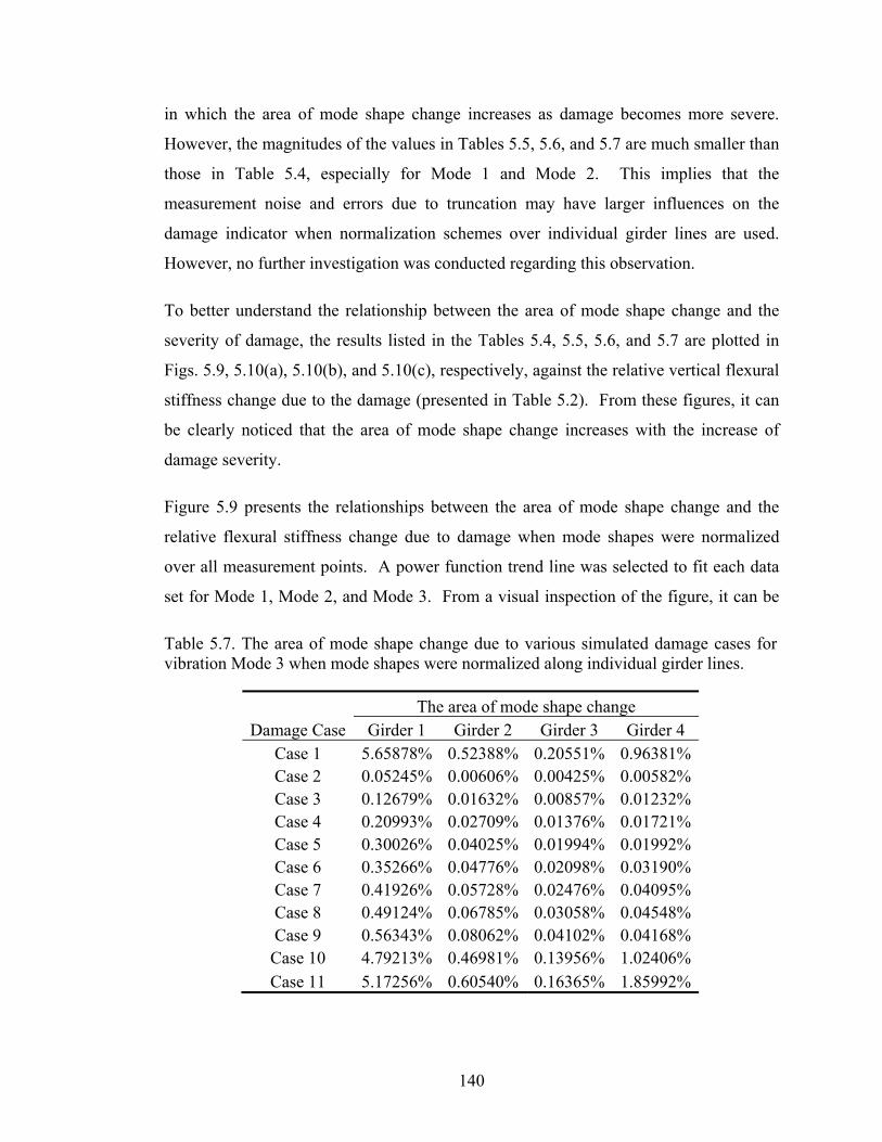
140
in which the area of mode shape change increases as damage becomes more severe.
However, the magnitudes of the values in Tables 5.5, 5.6, and 5.7 are much smaller than
those in Table 5.4, especially for Mode 1 and Mode 2. This implies that the
measurement noise and errors due to truncation may have larger influences on the
damage indicator when normalization schemes over individual girder lines are used.
However, no further investigation was conducted regarding this observation.
To better understand the relationship between the area of mode shape change and the
severity of damage, the results listed in the Tables 5.4, 5.5, 5.6, and 5.7 are plotted in
Figs. 5.9, 5.10(a), 5.10(b), and 5.10(c), respectively, against the relative vertical flexural
stiffness change due to the damage (presented in Table 5.2). From these figures, it can
be clearly noticed that the area of mode shape change increases with the increase of
damage severity.
Figure 5.9 presents the relationships between the area of mode shape change and the
relative flexural stiffness change due to damage when mode shapes were normalized
over all measurement points. A power function trend line was selected to fit each data
set for Mode 1, Mode 2, and Mode 3. From a visual inspection of the figure, it can be
Table 5.7. The area of mode shape change due to various simulated damage cases for vibration Mode 3 when mode shapes were normalized along individual girder lines.
The area of mode shape change Damage Case Girder 1 Girder 2 Girder 3 Girder 4
Case 1 5.65878% 0.52388% 0.20551% 0.96381% Case 2 0.05245% 0.00606% 0.00425% 0.00582% Case 3 0.12679% 0.01632% 0.00857% 0.01232% Case 4 0.20993% 0.02709% 0.01376% 0.01721% Case 5 0.30026% 0.04025% 0.01994% 0.01992% Case 6 0.35266% 0.04776% 0.02098% 0.03190% Case 7 0.41926% 0.05728% 0.02476% 0.04095% Case 8 0.49124% 0.06785% 0.03058% 0.04548% Case 9 0.56343% 0.08062% 0.04102% 0.04168% Case 10 4.79213% 0.46981% 0.13956% 1.02406% Case 11 5.17256% 0.60540% 0.16365% 1.85992%
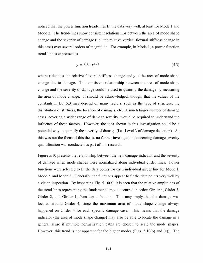
141
noticed that the power function tread-lines fit the data very well, at least for Mode 1 and
Mode 2. The trend-lines show consistent relationships between the area of mode shape
change and the severity of damage (i.e., the relative vertical flexural stiffness change in
this case) over several orders of magnitude. For example, in Mode 1, a power function
trend-line is expressed as
3.3 ∙ . [5.3]
where denotes the relative flexural stiffness change and is the area of mode shape
change due to damage. This consistent relationship between the area of mode shape
change and the severity of damage could be used to quantify the damage by measuring
the area of mode change. It should be acknowledged, though, that the values of the
constants in Eq. 5.3 may depend on many factors, such as the type of structure, the
distribution of stiffness, the location of damages, etc. A much larger number of damage
cases, covering a wider range of damage severity, would be required to understand the
influence of these factors. However, the idea shown in this investigation could be a
potential way to quantify the severity of damage (i.e., Level 3 of damage detection). As
this was not the focus of this thesis, no further investigation concerning damage severity
quantification was conducted as part of this research.
Figure 5.10 presents the relationship between the new damage indicator and the severity
of damage when mode shapes were normalized along individual girder lines. Power
functions were selected to fit the data points for each individual girder line for Mode 1,
Mode 2, and Mode 3. Generally, the functions appear to fit the data points very well by
a vision inspection. By inspecting Fig. 5.10(a), it is seen that the relative amplitudes of
the trend-lines representing the fundamental mode occurred in order: Girder 4, Girder 3,
Girder 2, and Girder 1, from top to bottom. This may imply that the damage was
located around Girder 4, since the maximum area of mode shape change always
happened on Girder 4 for each specific damage case. This means that the damage
indicator (the area of mode shape change) may also be able to locate the damage in a
general sense if multiple normalization paths are chosen to scale the mode shapes.
However, this trend is not apparent for the higher modes (Figs. 5.10(b) and (c)). The

142
main contribution of this new damage indicator is to detect the presence of damage,
especially for cases where large experimental uncertainties are involved. This is
discussed in the next chapter, where the resolutions of the various test procedures are
defined in a statistical manner.

143
y = 0.1573x0.7331
R² = 0.9481
0.01%
0.10%
1.00%
10.00%
100.00%
0.01% 0.10% 1.00% 10.00% 100.00%
Are
a of
mod
e sh
ape
chan
ge d
ue to
da
mag
e
Relative flexural stiffness change due to damage
Area change vs. Stiffness change
Trendline
y = 3.8321x1.1749
R² = 0.9962
0.01%
0.10%
1.00%
10.00%
100.00%
0.01% 0.10% 1.00% 10.00% 100.00%
Are
a of
mod
e sh
ape
chan
ge d
ue to
da
mag
e
Relative flexural stiffness change due to damage
Area change vs. Stiffness change
Trendline
y = 3.2995x1.2617
R² = 0.9945
0.01%
0.10%
1.00%
10.00%
100.00%
0.01% 0.10% 1.00% 10.00% 100.00%
Are
a of
mod
e sh
ape
chan
ge d
ue to
da
mag
e
Relative flexural stiffness change due to damage
Area change vs. Stiffness change
Trendline
Figure 5.9. Relationship between the area of mode shape change and the relative flexuralstiffness change due to damage for: (a) Mode 1, (b) Mode 2, and (c) Mode 3 when modeshapes were normalized over all measurement points.
(b)
(c)
(a)
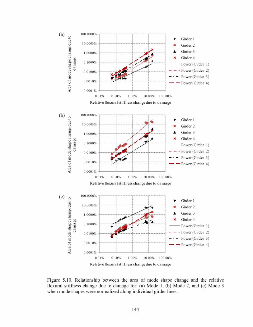
144
0.0001%
0.0010%
0.0100%
0.1000%
1.0000%
10.0000%
100.0000%
0.01% 0.10% 1.00% 10.00% 100.00%
Are
a of
mod
e sh
ape
chan
ge d
ue to
da
mag
e
Relative flexural stiffness change due to damage
Girder 1
Girder 2
Girder 3
Girder 4
Power (Girder 1)
Power (Girder 2)
Power (Girder 3)
Power (Girder 4)
0.0001%
0.0010%
0.0100%
0.1000%
1.0000%
10.0000%
100.0000%
0.01% 0.10% 1.00% 10.00% 100.00%
Are
a of
mod
e sh
ape
chan
ge d
ue to
da
mag
e
Relative flexural stiffness change due to damage
Girder 1
Girder 2
Girder 3
Girder 4
Power (Girder 1)
Power (Girder 2)
Power (Girder 3)
Power (Girder 4)
0.0001%
0.0010%
0.0100%
0.1000%
1.0000%
10.0000%
100.0000%
0.01% 0.10% 1.00% 10.00% 100.00%
Are
a of
mod
e sh
ape
chan
ge d
ue to
da
mag
e
Relative flexural stiffness change due to damage
Girder 1
Girder 2
Girder 3
Girder 4
Power (Girder 1)
Power (Girder 2)
Power (Girder 3)
Power (Girder 4)
Figure 5.10. Relationship between the area of mode shape change and the relativeflexural stiffness change due to damage for: (a) Mode 1, (b) Mode 2, and (c) Mode 3when mode shapes were normalized along individual girder lines.
(b)
(c)
(a)

145
CHAPTER 6. APPLICATION OF VBDD METHODS TO
THE MULTI-GIRDER BRIDGE SUPERSTRUCTURE
6.1 Overview
This chapter presents the application of various VBDD methods to the multi-girder
bridge model using the experimental data collected from both accelerometers and strain
gauges with both harmonic and white noise random excitation.
First, the distribution of the area of mode shape change is investigated when there is no
change in condition. Next, the resolution of various test protocols is defined and
calculated based on the statistical distribution of the area change in mode shape damage
indicator, expressed as threshold values which correspond to certain statistical
confidence levels. Then, detection of the presence of damage using the area of mode
shape change method is investigated in a statistical manner, based on the calculated
probability that there is no change in condition. Next, the detection of the presence of
damage using the area of mode shape change damage indicator is investigated based on
an alternative and simplified procedure by comparing the mean of the measurements
with the corresponding threshold values of the test protocols.
In the last part of this chapter, five commonly available VBDD indicators are used to
identify the location of damage after the presence of damage had been detected. The
performance of the VBDD indicators was investigated and compared while two
different normalization schemes were adopted.

146
6.2 Detection of the Presence of Damage Using the Area of Mode Shape Change
Damage Indicator
6.2.1 Overview
Ideally, two independent measurements of a particular mode shape for a structure in the
same condition would result in identical unit-area normalized mode shapes. However,
uncertainties inherent in the test procedures lead to variability in the measured mode
shapes obtained from separate data sets. Thus, a non-zero area of mode shape change
will be obtained even when the condition of the structure has not changed. As a result,
for the practical application of the VBDD methods, it is necessary to define the
resolutions of test procedures adopted. In other words, how large does the value of the
area of mode shape change have to be before one can say with confidence that damage
has occurred? The target of this investigation was to find a test protocol which has the
best resolution, therefore leading to the greatest likelihood of detecting the damage.
6.2.2 Distribution of the area of mode shape change when there is no change in
condition
Uncertainties inherent in the test protocols lead to a non-zero area of mode shape change
even when there is no change in the bridge’s physical condition. Also, the value of the
area of mode shape change, Δ , varies between different test samples. To quantify the
level of variation, it is necessary to investigate the statistical distribution of the area of
mode shape change.
For the current study, a total of 170 independent pairs of mode shapes from 85
independent mode shape measurements (i.e., five independent measurement sets for
each of 17 health states), were used to obtain the statistical variation of Δ , in which
each mode shape in the pair was obtained from the structure in an identical condition.
For each pair of mode shapes, and , the change in mode shape was first obtained
using Eq. 5.1, and the area of mode shape change, Δ , was then calculated using Eq.
5.2. In this manner, a total of 170 values of Δ were obtained to generate the mean and
the standard deviation of the area of mode shape change for an assumed normal
147
distribution, as well as to calculate the mean and standard deviation of the natural
logarithm of Δ for an assumed Log-Normal distribution.
To better understand the statistical characteristics of the population represented by the
tested sample group, Figs. 6.1 and 6.2 present comparisons of the actual cumulative
probability distributions and the assumed Normal and Log-Normal distributions of Δ
for the first mode with harmonic (Test Protocols 1 to 4, see Table 3.6) and white noise
excitation (Test Protocols 5 to 8), respectively. The actual cumulative distributions
were defined using the 170 calculated values, assuming that each value had an identical
probability of occurring. From a visual inspection of Figs. 6.1 and 6.2, it can be noticed
that both the Normal and Log-Normal distributions fit the actual distributions very well
for Test Protocols 2, 3, and 5 to 8. However, for Test Protocol 1 (Fig. 6.1(a)), the
Normal distribution fits the actual distribution better than the Log-Normal distribution,
where the Log-Normal distribution underestimated the cumulative probability for
specific Δ values in the higher probability region above 0.8. For Test Protocol 4 (Fig.
6.1(d)), the Log-Normal distribution looks somewhat better than the Normal distribution
to fit the actual distribution, where the Normal distribution underestimated the
cumulative probability for specific Δ in the middle probability region from 0.5 to 0.9.
More information about comparisons of the actual cumulative probability distribution
and assumed Normal and Log-Normal distributions is available in Appendix G for other
test protocols.
A quantitative comparison of the actual cumulative probability distributions and the
assumed Normal and Log-Normal distributions are listed in Table 6.1. In this table, the
sum of squares of the residuals (S.S.R.), regular residual standard deviation (or standard
error of estimate), and weighted residual standard deviation were used to quantify how
well the assumed Normal and Log-Normal distributions fit the actual cumulative
probability distributions. The best-fit curve is often assumed to be that which minimizes
the sum of squares of the residuals (i.e., the difference between observed and predicted
values). To reach a better physical understanding that is straightforward to compare to
the reading in the plots, the regular residual standard deviation (i.e., non-weighted) was
also used to compare the assumed and actual distributions. However, in cases where the

148
Figure 6.1. Comparison of the actual cumulative probability distributions and theassumed Normal and Log-Normal distributions of Δ , for Test Protocols: (a) 1, (b) 2,(c) 3, and (d) 4.
(a) (b)
(c) (d)
0.0
0.2
0.4
0.6
0.8
1.0
0.000 0.001 0.002 0.003 0.004 0.005
Cum
ulat
ive
prob
abili
ty
The area of mode shape change
Actual distribution
Normal distribution
Log-Normal distribution
0.0
0.2
0.4
0.6
0.8
1.0
0.000 0.001 0.002 0.003 0.004 0.005
Cum
ulat
ive
prob
abili
ty
The area of mode shape change
Actual distribution
Normal distribution
Log-Normal distribution
0.0
0.2
0.4
0.6
0.8
1.0
0.000 0.002 0.004 0.006 0.008 0.010
Cum
ulat
ive
prob
abili
ty
The area of mode shape change
Actual distribution
Normal distribution
Log-Normal distribution
0.0
0.2
0.4
0.6
0.8
1.0
0.000 0.010 0.020 0.030 0.040
Cum
ulat
ive
prob
abili
ty
The area of mode shape change
Actual distribution
Normal distribution
Log-Normal distribution

149
0.0
0.2
0.4
0.6
0.8
1.0
0.000 0.010 0.020 0.030 0.040 0.050
Cum
ulat
ive
prob
abili
ty
The area of mode shape change
Actual distribution
Normal distribution
Log-Normal distribution
0.0
0.2
0.4
0.6
0.8
1.0
0.000 0.005 0.010 0.015
Cum
ulat
ive
prob
abili
ty
The area of mode shape change
Actual distribution
Normal distribution
Log-Normal distribution
Figure 6.2. Comparison of the actual cumulative probability distributions and theassumed Normal and Log-Normal distributions of Δ , for Test Protocols: (a) 5, (b) 6,(c) 7, and (d) 8.
(a) (b)
(c) (d)
0.0
0.2
0.4
0.6
0.8
1.0
0.000 0.020 0.040 0.060 0.080
Cum
ulat
ive
prob
abili
ty
The area of mode shape change
Actual distribution
Normal distribution
Log-Normal distribution
0.0
0.2
0.4
0.6
0.8
1.0
0.000 0.050 0.100 0.150
Cum
ulat
ive
prob
abili
ty
The area of mode shape change
Actual distribution
Normal distribution
Log-Normal distribution

150
Table 6.1. Comparison of the actual cumulative probability distributions and the assumed Normal and Log-Normal distributions.
Test protocol
Normal distribution Log-Normal distribution S.S.R. R.R.S.D. W.R.S.D S.S.R. R.R.S.D. W.R.S.D
1 0.415 0.050 1.508 1.048 0.079 0.277 2 2.856 0.130 4.168 10.739 0.253 6.878 3 11.837 0.265 6.566 19.715 0.343 9.568 4 48.016 0.535 12.365 37.324 0.471 12.787 5 48.700 0.538 9.896 39.729 0.486 11.559 6 56.168 0.578 16.474 55.684 0.576 16.187 7 56.168 0.578 16.474 56.040 0.578 16.438 8 56.168 0.578 16.474 56.148 0.578 16.466 9 29.938 0.422 3.097 30.839 0.428 4.114 10 48.657 0.538 12.049 40.455 0.491 12.660 11 55.522 0.575 15.537 47.740 0.533 14.260 12 56.167 0.578 16.473 53.401 0.564 15.654 13 56.167 0.578 16.473 55.520 0.575 15.737 14 56.168 0.578 16.474 56.165 0.578 16.472 15 56.168 0.578 16.474 56.167 0.578 16.474 16 56.168 0.578 16.474 56.168 0.578 16.474 17 56.168 0.578 16.474 55.288 0.574 16.086 18 56.168 0.578 16.474 56.141 0.578 16.463 19 56.168 0.578 16.474 56.158 0.578 16.470 20 56.168 0.578 16.474 56.166 0.578 16.473 21 56.141 0.578 16.332 55.662 0.576 15.341 22 56.168 0.578 16.474 56.163 0.578 16.469 23 56.168 0.578 16.474 56.166 0.578 16.474 24 56.168 0.578 16.474 56.167 0.578 16.474 25 56.168 0.578 16.474 55.866 0.577 16.340 26 56.168 0.578 16.474 56.130 0.578 16.455 27 56.168 0.578 16.474 56.158 0.578 16.469 28 56.168 0.578 16.474 56.166 0.578 16.474
S.S.R. = Sum of square of the residuals; Residuals = differences between observed and predicted values; R.R.S.D. = Regular residual standard deviation (or standard error of estimate); W.R.S.D. = Weighted residual standard deviation (or weighted standard error of estimate).
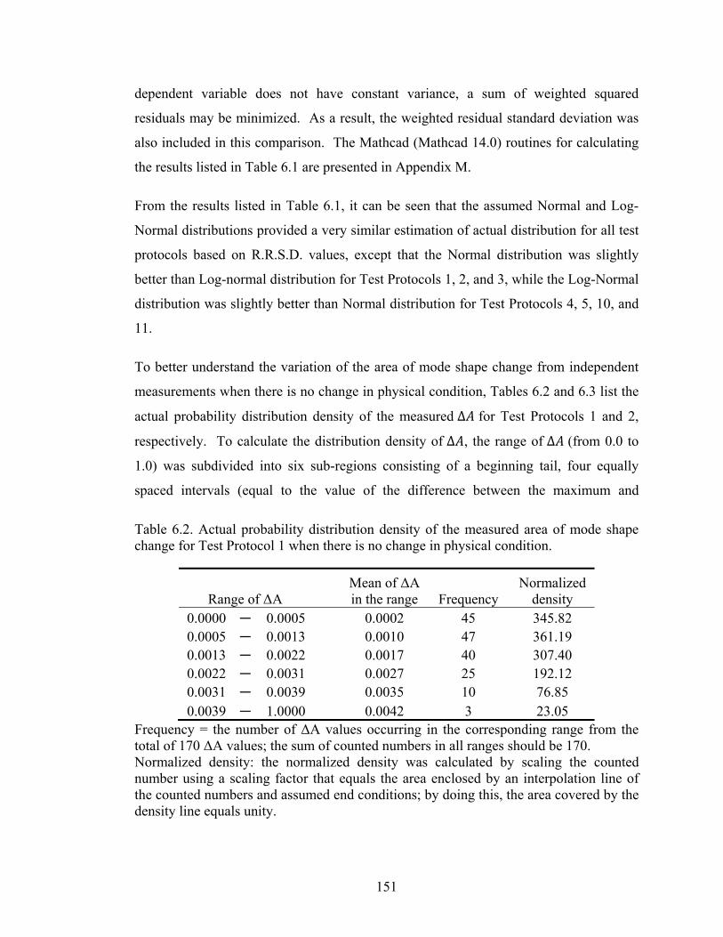
151
dependent variable does not have constant variance, a sum of weighted squared
residuals may be minimized. As a result, the weighted residual standard deviation was
also included in this comparison. The Mathcad (Mathcad 14.0) routines for calculating
the results listed in Table 6.1 are presented in Appendix M.
From the results listed in Table 6.1, it can be seen that the assumed Normal and Log-
Normal distributions provided a very similar estimation of actual distribution for all test
protocols based on R.R.S.D. values, except that the Normal distribution was slightly
better than Log-normal distribution for Test Protocols 1, 2, and 3, while the Log-Normal
distribution was slightly better than Normal distribution for Test Protocols 4, 5, 10, and
11.
To better understand the variation of the area of mode shape change from independent
measurements when there is no change in physical condition, Tables 6.2 and 6.3 list the
actual probability distribution density of the measured Δ for Test Protocols 1 and 2,
respectively. To calculate the distribution density of Δ , the range of Δ (from 0.0 to
1.0) was subdivided into six sub-regions consisting of a beginning tail, four equally
spaced intervals (equal to the value of the difference between the maximum and
Table 6.2. Actual probability distribution density of the measured area of mode shape change for Test Protocol 1 when there is no change in physical condition.
Range of ΔA Mean of ΔA in the range Frequency
Normalized density
0.0000 ― 0.0005 0.0002 45 345.82 0.0005 ― 0.0013 0.0010 47 361.19 0.0013 ― 0.0022 0.0017 40 307.40 0.0022 ― 0.0031 0.0027 25 192.12 0.0031 ― 0.0039 0.0035 10 76.85 0.0039 ― 1.0000 0.0042 3 23.05
Frequency = the number of ΔA values occurring in the corresponding range from the total of 170 ΔA values; the sum of counted numbers in all ranges should be 170. Normalized density: the normalized density was calculated by scaling the counted number using a scaling factor that equals the area enclosed by an interpolation line of the counted numbers and assumed end conditions; by doing this, the area covered by the density line equals unity.

152
minimum values of readings, divided by five), and an ending tail. The six sub-ranges
were selected in this case to balance the variation requirements for both Δ and
probability density of each specific Δ . For example, at one extreme, if no subdivision
and only one range is used, only one averaged Δ value (with a counted number of 170)
can be produced to generate the density function, which has no variation in Δ , and is
therefore meaningless. At the other extreme, if too many sub-ranges are used (at least
170 sub-ranges), only one sample may be available in each sub-range, which then has
no variation in the probability density (i.e., each sub-range has only one Δ included
and frequency is one for this sub-range). The number of Δ values in each range was
counted, a value which was defined as the frequency of Δ , and recorded together with
the mean value of Δ that occurred in the corresponding range. The sum of frequency
in all ranges should equal to the total number of Δ values of 170. To define the
probability density function, the counted number (or frequency) had to be normalized in
order that the area covered by the probability density function was equal to unity. As a
result, the counted numbers (or frequency) were scaled using a scaling factor equal to
the area covered by a line interpolated from the data points and based on assumed end
conditions. In this case, to simplify the process, the frequency was assumed to be zero
Table 6.3. Actual probability distribution density of the measured area of mode shape change for Test Protocol 2 when there is no change in physical condition.
Range of ΔA Mean of ΔA in the range Frequency
Normalized density
0.0000 ― 0.0011 0.0009 29 240.77 0.0011 ― 0.0018 0.0014 87 722.30 0.0018 ― 0.0026 0.0022 38 315.49 0.0026 ― 0.0033 0.0030 8 66.42 0.0033 ― 0.0041 0.0037 5 41.51 0.0041 ― 1.0000 0.0043 3 24.91
Frequency = the number of ΔA values occurring in the corresponding range from the total of 170 ΔA values; the sum of counted numbers in all ranges should be 170. Normalized density: the normalized density was calculated by scaling the counted number using a scaling factor that equals the area enclosed by an interpolation line of the counted numbers and assumed end conditions; by doing this, the area covered by the density line equals unity.

153
at the Δ value of zero, which means that the probability of producing two mode shapes
that are exactly the same from two independent measurements under practical testing
conditions is negligible. Another boundary condition that was assumed was that the
probability of producing a large value of Δ (i.e., significantly large changes in
condition) is exceedingly small. In this case, the frequency was assumed to be 0.1 (i.e.,
one tenth of one count) for a Δ value equal to twice the maximum of the 170 Δ
values. The detailed Mathcad (Mathcad 14.0) calculations are presented in Appendix M.
The probability density results listed in Tables 6.2 and 6.3 are also plotted in Fig. 6.3,
together with the assumed Normal and Log-Normal distributions, where the mean and
standard deviation of the assumed distributions were calculated from the 170 Δ values,
as described in previous paragraphs for Figs. 6.1 and 6.2. Also, the 95th percentile of the
assumed Normal and Log-Normal distribution are plotted in Figs. 6.3. In a similar way,
Figs. 6.4, 6.5, and 6.6 present comparisons of the probability density between the actual
distribution and the assumed Normal and Log-Normal distributions of Δ for Test
Protocols 3 to 8. The comparisons of probability density for all other test protocols are
presented in Appendix G.
From a visual inspection of the results shown in Figs. 6.3 to 6.6, it can be seen that
Normal distribution fits the actual distribution slightly better than Log-Normal
distribution for Test Protocols 1 and 6, while the Log-Normal distribution fits slightly
better than Normal distribution for Test Protocols 2, 4, and 5. Generally, the actual
distributions were located between the assumed Normal and Log-Normal distributions.
Considering the 95th percentile values, the values for Log-Normal distribution were
generally larger than those for Normal distribution, except for Test Protocols 3 and 4.
This suggests that using the 95th percentile from Log-Normal distribution as the
threshold value, as described in the next section, may be more suitable for damage
detection from a conservative point of view. Detailed discussion on this is available in
Section 6.2.3 and 6.2.4.

154
Figure 6.3. Comparison of the probability density between the actual distribution andthe assumed Normal and Log-Normal distributions of Δ , for Test Protocols: (a) 1 and(b) 2.
(a)
(b)
0 0.002 0.004 0.006 0.0080
200
400
600
800
Assumed Normal distributionAssumed Log-Normal distribution95th percentile of Normal distribution95th percentile of Log-Normal distributionActual distribution
The area of mode shape change
Dis
trib
utio
n de
nsit
y
0 0.002 0.004 0.006 0.0080
200
400
600
800
The area of mode shape change
Dis
trib
utio
n de
nsit
y
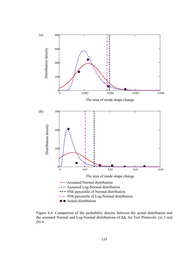
155
Figure 6.4. Comparison of the probability density between the actual distribution andthe assumed Normal and Log-Normal distributions of Δ , for Test Protocols: (a) 3 and(b) 4.
(a)
(b)
0 0.01 0.02 0.03 0.040
100
200
300
Assumed Normal distributionAssumed Log-Normal distribution95th percentile of Normal distribution95th percentile of Log-Normal distributionActual distribution
The area of mode shape change
Dis
trib
utio
n de
nsit
y
0 0.002 0.004 0.006 0.0080
200
400
600
800
The area of mode shape change
Dis
trib
utio
n de
nsit
y

156
Figure 6.5. Comparison of the probability density between the actual distribution andthe assumed Normal and Log-Normal distributions of Δ , for Test Protocols: (a) 5 and(b) 6.
(a)
(b)
0 0.005 0.01 0.015 0.020
100
200
300
The area of mode shape change
Dis
trib
utio
n de
nsit
y
0 0.02 0.04 0.06 0.080
20
40
60
80
100
Assumed Normal distributionAssumed Log-Normal distribution95th percentile of Normal distribution95th percentile of Log-Normal distributionActual distribution
The area of mode shape change
Dis
trib
utio
n de
nsit
y
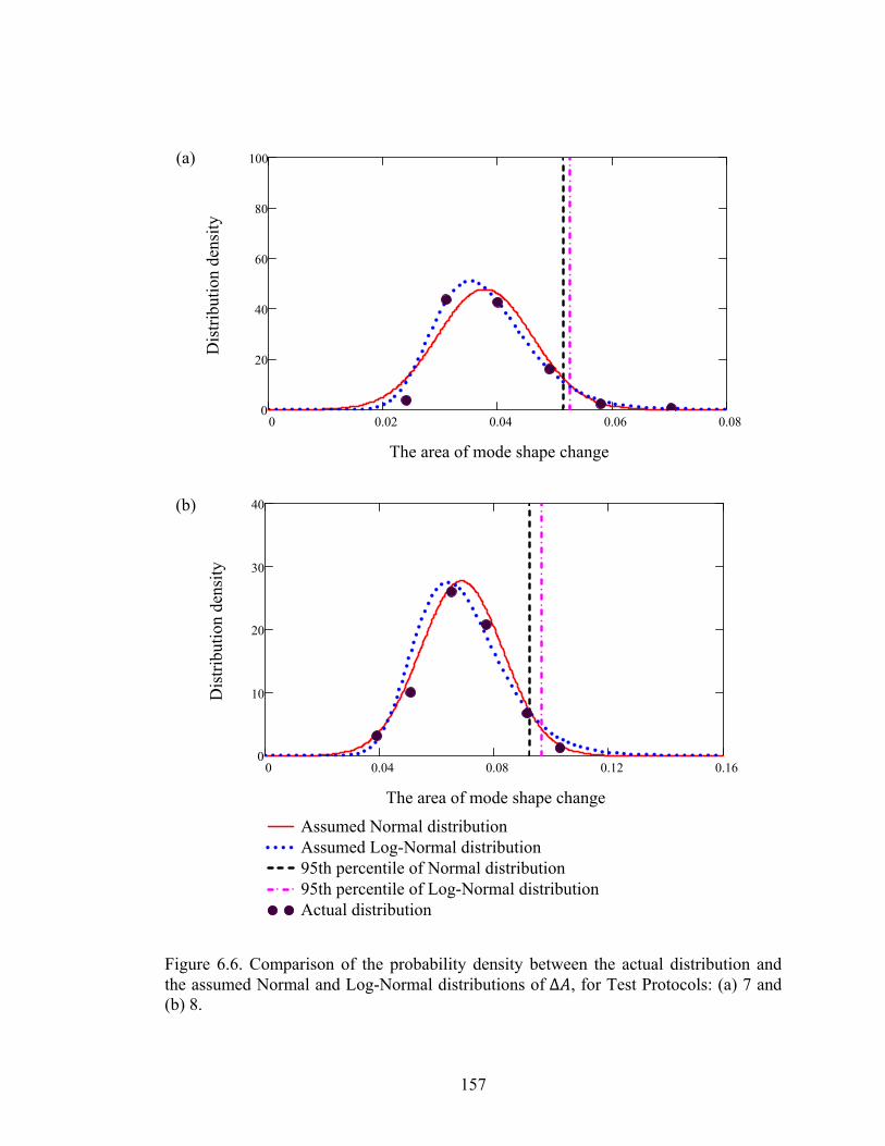
157
Figure 6.6. Comparison of the probability density between the actual distribution andthe assumed Normal and Log-Normal distributions of Δ , for Test Protocols: (a) 7 and(b) 8.
(a)
(b)
0 0.02 0.04 0.06 0.080
20
40
60
80
100
The area of mode shape change
Dis
trib
utio
n de
nsit
y
0 0.04 0.08 0.12 0.160
10
20
30
40
Assumed Normal distributionAssumed Log-Normal distribution95th percentile of Normal distribution95th percentile of Log-Normal distributionActual distribution
The area of mode shape change
Dis
trib
utio
n de
nsit
y
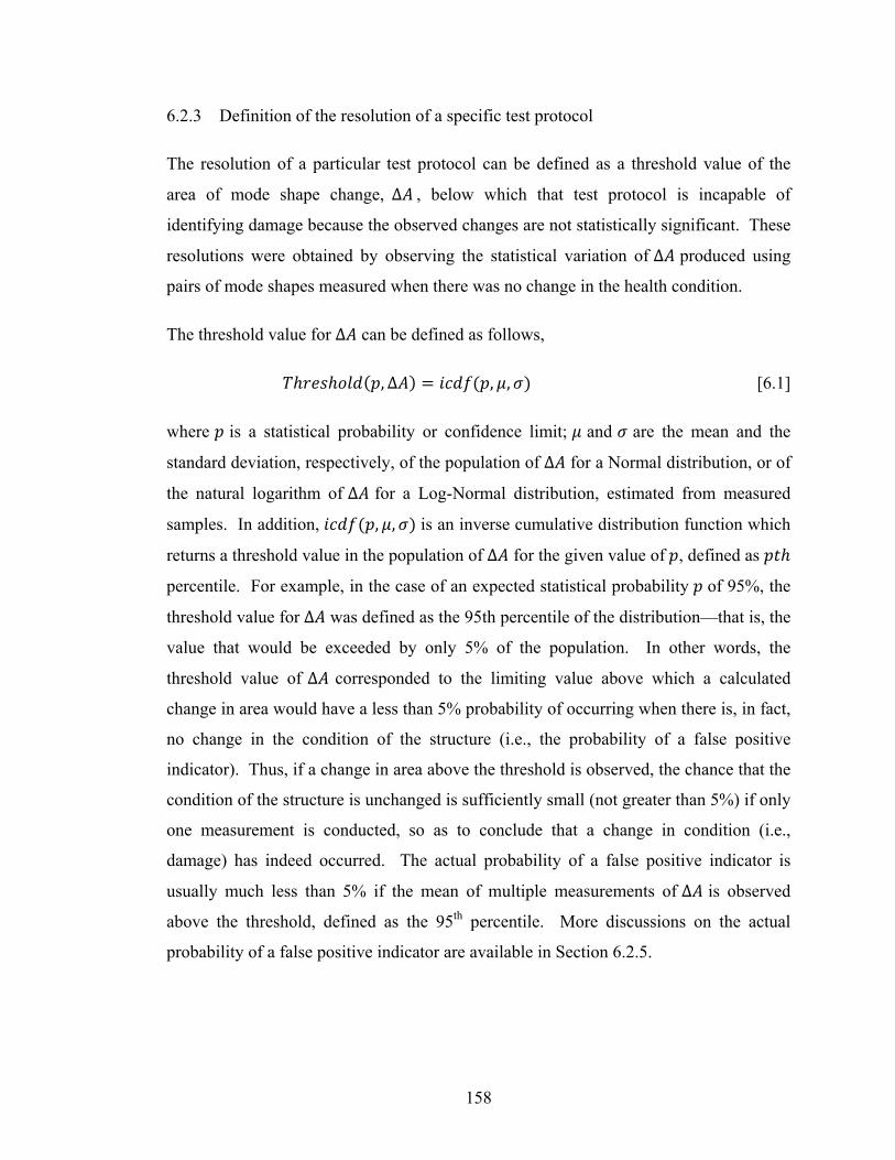
158
6.2.3 Definition of the resolution of a specific test protocol
The resolution of a particular test protocol can be defined as a threshold value of the
area of mode shape change, Δ , below which that test protocol is incapable of
identifying damage because the observed changes are not statistically significant. These
resolutions were obtained by observing the statistical variation of Δ produced using
pairs of mode shapes measured when there was no change in the health condition.
The threshold value for Δ can be defined as follows,
, ∆ , , [6.1]
where is a statistical probability or confidence limit; and are the mean and the
standard deviation, respectively, of the population of ∆ for a Normal distribution, or of
the natural logarithm of ∆ for a Log-Normal distribution, estimated from measured
samples. In addition, , , is an inverse cumulative distribution function which
returns a threshold value in the population of ∆ for the given value of , defined as
percentile. For example, in the case of an expected statistical probability of 95%, the
threshold value for ∆ was defined as the 95th percentile of the distribution—that is, the
value that would be exceeded by only 5% of the population. In other words, the
threshold value of Δ corresponded to the limiting value above which a calculated
change in area would have a less than 5% probability of occurring when there is, in fact,
no change in the condition of the structure (i.e., the probability of a false positive
indicator). Thus, if a change in area above the threshold is observed, the chance that the
condition of the structure is unchanged is sufficiently small (not greater than 5%) if only
one measurement is conducted, so as to conclude that a change in condition (i.e.,
damage) has indeed occurred. The actual probability of a false positive indicator is
usually much less than 5% if the mean of multiple measurements of Δ is observed
above the threshold, defined as the 95th percentile. More discussions on the actual
probability of a false positive indicator are available in Section 6.2.5.
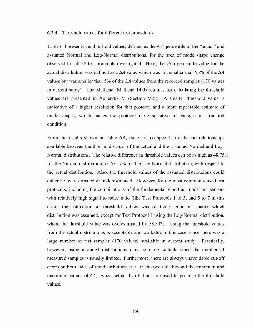
159
6.2.4 Threshold values for different test procedures
Table 6.4 presents the threshold values, defined as the 95th percentile of the “actual” and
assumed Normal and Log-Normal distributions, for the area of mode shape change
observed for all 28 test protocols investigated. Here, the 95th percentile value for the
actual distribution was defined as a Δ value which was not smaller than 95% of the Δ
values but was smaller than 5% of the Δ values from the recorded samples (170 values
in current study). The Mathcad (Mathcad 14.0) routines for calculating the threshold
values are presented in Appendix M (Section M.5). A smaller threshold value is
indicative of a higher resolution for that protocol and a more repeatable estimate of
mode shapes, which makes the protocol more sensitive to changes in structural
condition.
From the results shown in Table 6.4, there are no specific trends and relationships
available between the threshold values of the actual and the assumed Normal and Log-
Normal distributions. The relative difference in threshold values can be as high as 48.75%
for the Normal distribution, or 67.17% for the Log-Normal distribution, with respect to
the actual distribution. Also, the threshold values of the assumed distributions could
either be overestimated or underestimated. However, for the most commonly used test
protocols, including the combinations of the fundamental vibration mode and sensors
with relatively high signal to noise ratio (like Test Protocols 1 to 3, and 5 to 7 in this
case), the estimation of threshold values was relatively good no matter which
distribution was assumed, except for Test Protocol 1 using the Log-Normal distribution,
where the threshold value was overestimated by 58.39%. Using the threshold values
from the actual distributions is acceptable and workable in this case, since there was a
large number of test samples (170 values) available in current study. Practically,
however, using assumed distributions may be more suitable since the number of
measured samples is usually limited. Furthermore, there are always unavoidable cut-off
errors on both sides of the distributions (i.e., in the two tails beyond the minimum and
maximum values of Δ ), when actual distributions are used to produce the threshold
values.

160
Table 6.4. Threshold values of the area of mode shape change for different test protocols, defined as the 95th percentile of the actual and assumed distributions.
Test protocol Actual Normal
Relative Difference
Log-Normal
Relative Difference
1 0.0036 0.0032 -11.51% 0.0057 58.39% 2 0.0033 0.0029 -11.04% 0.0029 -9.46% 3 0.0043 0.0040 -6.81% 0.0038 -11.48% 4 0.0179 0.0139 -22.69% 0.0104 -42.21% 5 0.0097 0.0089 -8.21% 0.0096 -0.88% 6 0.0362 0.0353 -2.30% 0.0372 2.99% 7 0.0518 0.0515 -0.51% 0.0527 1.85% 8 0.0930 0.0924 -0.67% 0.0966 3.86% 9 0.0509 0.0451 -11.52% 0.0852 67.17% 10 0.0203 0.0195 -3.72% 0.0210 3.32% 11 0.0291 0.0251 -13.63% 0.0264 -9.21% 12 0.0484 0.0448 -7.39% 0.0485 0.30% 13 0.1074 0.1597 48.75% 0.1130 5.23% 14 0.5867 0.4777 -18.58% 0.5290 -9.83% 15 0.5113 0.4757 -6.96% 0.5221 2.11% 16 0.6775 0.6542 -3.43% 0.7149 5.52% 17 0.0462 0.0455 -1.63% 0.0478 3.47% 18 0.1370 0.1317 -3.89% 0.1323 -3.41% 19 0.1857 0.1728 -6.96% 0.1801 -3.01% 20 0.2700 0.2595 -3.86% 0.2694 -0.21% 21 0.2480 0.2300 -7.25% 0.3212 29.53% 22 0.5039 0.4096 -18.71% 0.4024 -20.13% 23 0.6035 0.4369 -27.61% 0.4160 -31.07% 24 0.5865 0.5150 -12.19% 0.5335 -9.05% 25 0.0516 0.0501 -2.89% 0.0531 2.94% 26 0.1967 0.1824 -7.27% 0.1893 -3.77% 27 0.2536 0.2182 -13.96% 0.2228 -12.14% 28 0.3601 0.3325 -7.67% 0.3485 -3.22%
Relative Difference = Relative difference in the threshold values between the assumed distribution and actual distribution, calculated using (assumed-actual)/actual;

161
To better understand the trends of threshold values and the influence of the level of
confidence on the threshold values, the 90th percentile of the actual and assumed Normal
and Log-Normal distributions for the area of mode shape change observed for all 28 test
protocols were calculated and are listed in Table 6.5. As expected, all values in Table
6.5 are smaller than the corresponding ones in Table 6.4 since the confidence level was
decreased from 95% to 90%. However, the general trends for different sensor schemes
and excitation types remained similar to those found in Table 6.4.
To simplify the concepts involved, only the threshold values from the assumed Log-
Normal distribution are discussed in detail in the following paragraphs in this sub-
section. To clarify the influence of excitation and sensor types on the threshold values,
the threshold values listed in Table 6.4 for the Log-Normal distribution are reorganized
and presented in Table 6.6 along with an explicit name of components for the various
test protocols.
The results presented in Table 6.6 show that when white noise excitation was used, the
use of the fundamental vibration mode obtained by acceleration measurements (or Test
Protocol 5) was clearly superior to all other protocols (or Test Protocols 6 to 8).
Measurement of the fundamental mode using the bottom strain gauges (or Test Protocol
6) resulted in the next most reliable results, although the threshold value was around
four times that obtained using acceleration measurements. The use of acceleration
measurements to obtain higher modes, also produced better resolutions than those
obtained by strain measurements, with bottom strain measurements producing the next
best results. However, with the possible exception of measurements of modes 3 and 5
using accelerometers, threshold values achieved for higher modes were high enough that
the protocols would likely be insensitive to all but the most severe of damage cases.
The use of harmonic excitation to measure the fundamental vibration mode resulted in
the lowest threshold values of all protocols considered, with all four instrumentation
schemes producing similar results (the threshold value was only slightly higher for the
top strain gauges, which were found to produce much lower signal-to-noise ratios than
other sensor schemes). These protocols can therefore be considered to be the most

162
Table 6.5. Threshold values of the area of mode shape change for different test protocols, defined as the 90th percentile of the actual and assumed distributions.
Test protocol Actual Normal
Relative Difference
Log-Normal
Relative Difference
1 0.0029 0.0028 -3.24% 0.0038 31.61% 2 0.0025 0.0026 6.41% 0.0026 3.77% 3 0.0035 0.0036 4.22% 0.0033 -3.63% 4 0.0065 0.0120 85.34% 0.0085 32.23% 5 0.0082 0.0081 -0.88% 0.0083 1.26% 6 0.0321 0.0331 3.16% 0.0340 5.82% 7 0.0488 0.0485 -0.74% 0.0487 -0.22% 8 0.0876 0.0871 -0.51% 0.0891 1.75% 9 0.0390 0.0390 0.03% 0.0518 32.78% 10 0.0175 0.0171 -2.28% 0.0162 -7.59% 11 0.0229 0.0221 -3.45% 0.0209 -8.77% 12 0.0462 0.0394 -14.65% 0.0381 -17.48% 13 0.0744 0.1354 82.06% 0.0878 18.04% 14 0.4559 0.4232 -7.18% 0.4221 -7.42% 15 0.4308 0.4257 -1.18% 0.4296 -0.28% 16 0.6020 0.5931 -1.48% 0.6073 0.89% 17 0.0371 0.0411 10.88% 0.0409 10.26% 18 0.1141 0.1194 4.64% 0.1151 0.88% 19 0.1600 0.1574 -1.67% 0.1565 -2.19% 20 0.2305 0.2379 3.22% 0.2374 3.00% 21 0.2082 0.2022 -2.89% 0.2338 12.29% 22 0.3419 0.3593 5.09% 0.3230 -5.53% 23 0.3599 0.3853 7.05% 0.3424 -4.86% 24 0.4612 0.4604 -0.18% 0.4452 -3.48% 25 0.0464 0.0463 -0.16% 0.0472 1.84% 26 0.1737 0.1618 -6.83% 0.1546 -11.00% 27 0.2018 0.1956 -3.07% 0.1879 -6.88% 28 0.3037 0.3013 -0.79% 0.2993 -1.46%
Relative Difference = Relative difference in the threshold values between the assumed distribution and actual distribution, calculated using (assumed-actual)/actual;

163
sensitive to changes in structural condition, and therefore the most likely to identify the
presence of damage. Interestingly, the protocols making use of strain gauge
measurements (especially from the bottom and middle gauges) typically resulted in
lower threshold values than those using accelerometer measurements when harmonic
excitation was used, despite the fact that mode shapes generated from accelerometer
data have previously been shown to be more repeatable than those produced using the
strain gauge data (see the results in Chapter 4). This might be explained in part by the
fact that multiple independent setups were required for acceleration measurements due
to the limited number of accelerometers available, whereas the permanently installed
strain gauges required only a single setup.
6.2.5 Detection of the presence of damage using the area of mode shape change
method based on the calculated probability values
As described in Section 3.4, sixteen single damage cases were induced in the bridge
model after the undamaged dynamic properties had been established (see Table 3.5).
For each damage case, the area of mode shape change was calculated for all five
vibration modes using Eqs. 5.1 and 5.2, in which five separate tests were conducted to
measure each of the damaged and undamaged unit-area normalized mode shape vectors,
and , respectively. As a result, a total of 25 values of area of mode shape change
were generated by the 25 independent pairs of damaged and undamaged mode shape
vectors for each vibration mode and each damage case. Table 6.7 presents a sample of
Table 6.6. Threshold values of area of mode shape change for different test protocols, defined as the 95th percentile of the Log-Normal distribution, expressed as percentage of total area under the original unit-area normalized mode shape.
White noise excitation Harmonic excitationInstrumentation Mode 1 Mode 2 Mode 3 Mode 4 Mode 5 Mode 1 Mode 2 Acceleration 0.96% 11.30% 4.78% 32.12% 5.31% 0.57% 8.52% Bottom strain 3.72% 52.90% 13.23% 40.24% 18.93% 0.29% 2.10% Middle strain 5.27% 52.21% 18.01% 41.60% 22.28% 0.38% 2.64% Top strain 9.66% 71.49% 26.94% 53.35% 34.85% 1.04% 4.85%
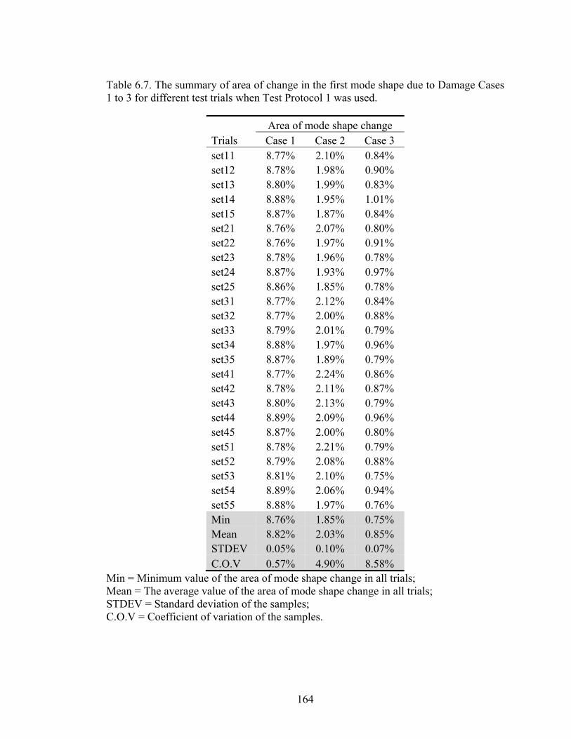
164
Table 6.7. The summary of area of change in the first mode shape due to Damage Cases 1 to 3 for different test trials when Test Protocol 1 was used.
Area of mode shape change Trials Case 1 Case 2 Case 3 set11 8.77% 2.10% 0.84% set12 8.78% 1.98% 0.90% set13 8.80% 1.99% 0.83% set14 8.88% 1.95% 1.01% set15 8.87% 1.87% 0.84% set21 8.76% 2.07% 0.80% set22 8.76% 1.97% 0.91% set23 8.78% 1.96% 0.78% set24 8.87% 1.93% 0.97% set25 8.86% 1.85% 0.78% set31 8.77% 2.12% 0.84% set32 8.77% 2.00% 0.88% set33 8.79% 2.01% 0.79% set34 8.88% 1.97% 0.96% set35 8.87% 1.89% 0.79% set41 8.77% 2.24% 0.86% set42 8.78% 2.11% 0.87% set43 8.80% 2.13% 0.79% set44 8.89% 2.09% 0.96% set45 8.87% 2.00% 0.80% set51 8.78% 2.21% 0.79% set52 8.79% 2.08% 0.88% set53 8.81% 2.10% 0.75% set54 8.89% 2.06% 0.94% set55 8.88% 1.97% 0.76% Min 8.76% 1.85% 0.75% Mean 8.82% 2.03% 0.85% STDEV 0.05% 0.10% 0.07% C.O.V 0.57% 4.90% 8.58%
Min = Minimum value of the area of mode shape change in all trials; Mean = The average value of the area of mode shape change in all trials; STDEV = Standard deviation of the samples; C.O.V = Coefficient of variation of the samples.

165
the calculated results for Damage Case 1, Case 2, and Case 3, in which only
accelerometer data with harmonic excitation were used to generate the results (i.e., Test
Protocol 1). The statistical values, including the minimum, mean, standard deviation,
and coefficient of variation of the Δ values are also listed in Table 6.7. It can be seen
that all values listed in Table 6.7 exceed the 95th percentile value shown in Table 6.6
(0.57%) for this test protocol, meaning that all three damage cases could be detected at
least a confidence level of 95%. The results for all damage cases and Test Protocols 1
to 8 are included in Appendix H.
It was assumed that the set of 25 values of Δ also formed a sample from a population
with a Normal or Log-Normal distribution, in a similar manner to that defined for the set
of 170 values of Δ when there was no change in physical condition, as described
previously. Now, two distributions were defined. One distribution was estimated using
170 values of Δ when there was no change in condition, and the other was estimated
using 25 values of Δ when there was (or may have been) a change in condition.
Figures 6.7 and 6.8 present the two distributions with the assumed Normal and Log-
Normal distributions, respectively, for Damage Cases 1 to 3, when Test Protocol 1 was
used. Both figures show similar results. The two groups shown in the two figures (one
for the undamaged group and the other for the damaged group) are well separated from
each other for Damage Cases 1 and 2; in addition, the distance between the mean values
of two groups is relatively large for Damage Cases 1 and 2. For Damage Case 3, there
is only a small region of intersection between the distribution density lines of the two
groups. As a result, one can confidently say that the two groups are from different
populations. This means that there has been a change in condition with a relatively high
confidence. Similar figures for other damage cases are presented in Appendix H.
Using the two distributions, it is possible to calculate the probability that the second
value (from damaged group) exceeds the first one (from undamaged group) (i.e., the
probability that there has been a change in condition). Conversely, one could calculate
the probability that the second value does not exceed the first (i.e., the probability that
there is no change in condition). The Mathcad (Mathcad 14.0) routines for calculating
the probabilities are presented in Appendix M (Section M.5).

166
Figure 6.7. Comparison of Normal distributions of the area of mode shape change forthe undamaged group of 170 pairs and the damaged group of 25 data pairs for DamageCase: (a) 1, (b) 2, and (c) 3, when the Test Protocol 1 was used.
(a)
(b)
(c)
0.01 0 0.01 0.02 0.03 0.04 0.05 0.06 0.07 0.08 0.09 0.10
200
400
600
800
The area of mode shape change
Dis
trib
utio
n de
nsit
y
0.01 0 0.01 0.02 0.03 0.04 0.05 0.06 0.07 0.08 0.09 0.10
200
400
600
800
The area of mode shape change
Dis
trib
utio
n de
nsit
y
0.01 0 0.01 0.02 0.03 0.04 0.05 0.06 0.07 0.08 0.09 0.10
200
400
600
800
Distribution of undamaged groupDistribution of damaged group90th percentile of undamaged group95th percentile of undamaged group
The area of mode shape change
Dis
trib
utio
n de
nsit
y
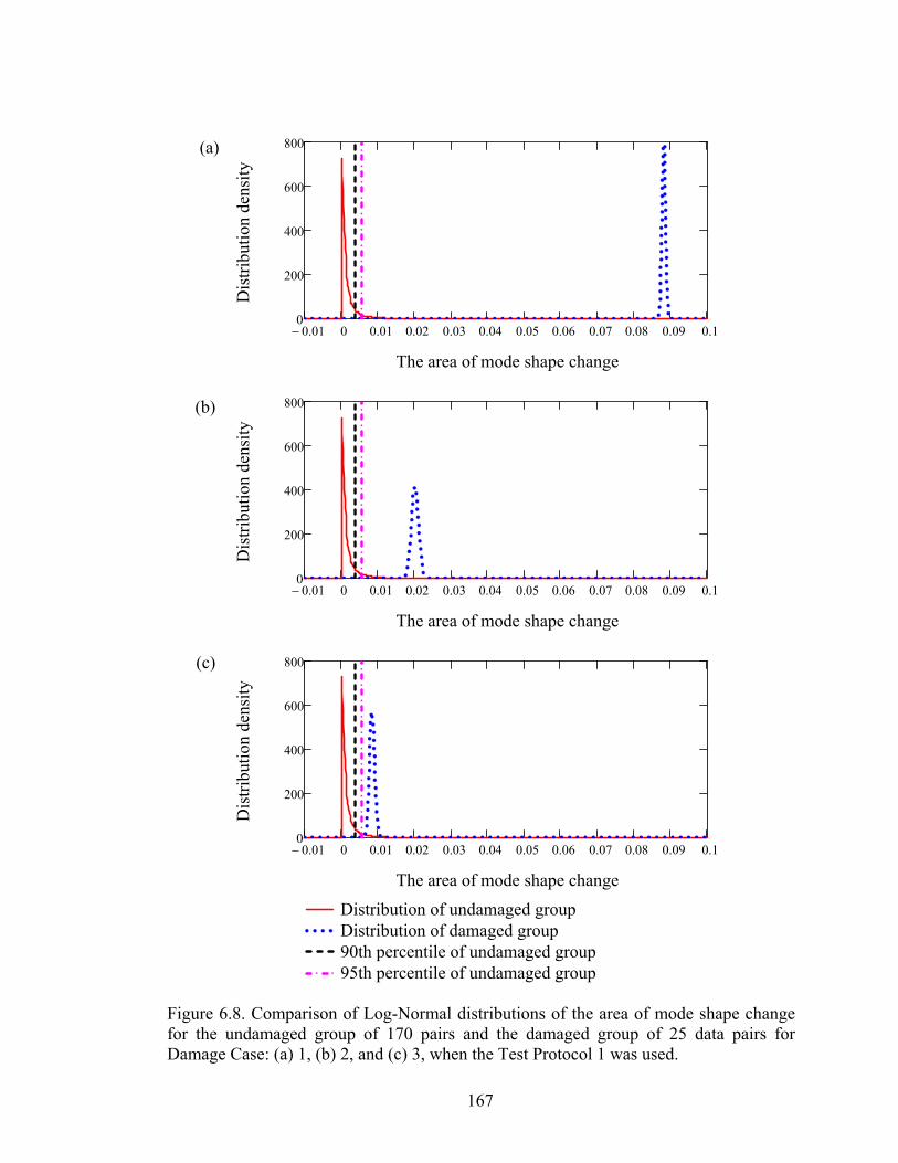
167
Figure 6.8. Comparison of Log-Normal distributions of the area of mode shape changefor the undamaged group of 170 pairs and the damaged group of 25 data pairs forDamage Case: (a) 1, (b) 2, and (c) 3, when the Test Protocol 1 was used.
(a)
(b)
(c)
0.01 0 0.01 0.02 0.03 0.04 0.05 0.06 0.07 0.08 0.09 0.10
200
400
600
800
The area of mode shape change
Dis
trib
utio
n de
nsit
y
0.01 0 0.01 0.02 0.03 0.04 0.05 0.06 0.07 0.08 0.09 0.10
200
400
600
800
The area of mode shape change
Dis
trib
utio
n de
nsit
y
0.01 0 0.01 0.02 0.03 0.04 0.05 0.06 0.07 0.08 0.09 0.10
200
400
600
800
Distribution of undamaged groupDistribution of damaged group90th percentile of undamaged group95th percentile of undamaged group
The area of mode shape change
Dis
trib
utio
n de
nsit
y
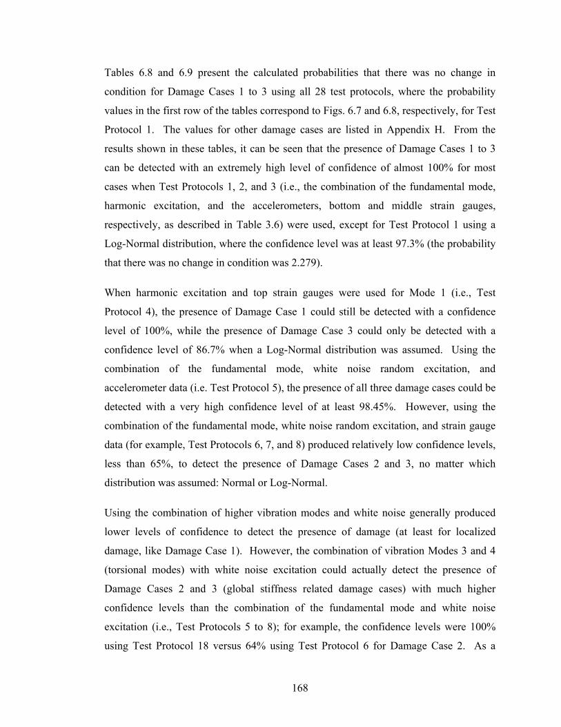
168
Tables 6.8 and 6.9 present the calculated probabilities that there was no change in
condition for Damage Cases 1 to 3 using all 28 test protocols, where the probability
values in the first row of the tables correspond to Figs. 6.7 and 6.8, respectively, for Test
Protocol 1. The values for other damage cases are listed in Appendix H. From the
results shown in these tables, it can be seen that the presence of Damage Cases 1 to 3
can be detected with an extremely high level of confidence of almost 100% for most
cases when Test Protocols 1, 2, and 3 (i.e., the combination of the fundamental mode,
harmonic excitation, and the accelerometers, bottom and middle strain gauges,
respectively, as described in Table 3.6) were used, except for Test Protocol 1 using a
Log-Normal distribution, where the confidence level was at least 97.3% (the probability
that there was no change in condition was 2.279).
When harmonic excitation and top strain gauges were used for Mode 1 (i.e., Test
Protocol 4), the presence of Damage Case 1 could still be detected with a confidence
level of 100%, while the presence of Damage Case 3 could only be detected with a
confidence level of 86.7% when a Log-Normal distribution was assumed. Using the
combination of the fundamental mode, white noise random excitation, and
accelerometer data (i.e. Test Protocol 5), the presence of all three damage cases could be
detected with a very high confidence level of at least 98.45%. However, using the
combination of the fundamental mode, white noise random excitation, and strain gauge
data (for example, Test Protocols 6, 7, and 8) produced relatively low confidence levels,
less than 65%, to detect the presence of Damage Cases 2 and 3, no matter which
distribution was assumed: Normal or Log-Normal.
Using the combination of higher vibration modes and white noise generally produced
lower levels of confidence to detect the presence of damage (at least for localized
damage, like Damage Case 1). However, the combination of vibration Modes 3 and 4
(torsional modes) with white noise excitation could actually detect the presence of
Damage Cases 2 and 3 (global stiffness related damage cases) with much higher
confidence levels than the combination of the fundamental mode and white noise
excitation (i.e., Test Protocols 5 to 8); for example, the confidence levels were 100%
using Test Protocol 18 versus 64% using Test Protocol 6 for Damage Case 2. As a

169
Table 6.8. The probability that there was no change in condition using the assumed Normal distributions (i.e., the probability that the Δ value obtained when there was a change in the condition did not exceed those that obtained when there was no change in condition), for Damage Cases 1 to 3 using all 28 Test Protocols.
Test Protocol
Damage Case
Case 1 Case 2 Case 3 1 0.000% 0.000% 0.000% 2 0.000% 0.000% 0.000% 3 0.000% 0.000% 0.000% 4 0.000% 4.412% 0.001% 5 0.000% 1.269% 0.292% 6 0.012% 35.924% 45.264% 7 4.616% 57.933% 48.554% 8 20.766% 49.092% 61.447% 9 0.000% 0.000% 4.084% 10 0.000% 0.000% 2.612% 11 0.000% 0.000% 4.303% 12 0.000% 0.000% 18.636% 13 25.462% 64.898% 62.606% 14 49.884% 75.615% 76.095% 15 47.427% 77.188% 77.093% 16 62.880% 85.769% 82.425% 17 0.001% 0.000% 1.556% 18 2.437% 0.000% 0.005% 19 11.748% 0.000% 0.320% 20 29.171% 0.000% 23.045% 21 14.696% 0.000% 3.534% 22 13.143% 0.170% 1.826% 23 14.823% 0.206% 3.209% 24 18.462% 0.544% 8.157% 25 16.268% 3.276% 0.007% 26 45.442% 49.606% 28.135% 27 42.437% 47.934% 35.181% 28 52.922% 52.050% 61.713%

170
Table 6.9. The probability that there was no change in condition using the assumed Log-Normal distributions (i.e., the probability that the Δ value obtained when there was a change in the condition did not exceed those that obtained when there was no change in condition), for Damage Cases 1 to 3 using all 28 Test Protocols.
Test Protocol
Damage Case
Case 1 Case 2 Case 3 1 0.002% 0.272% 2.279% 2 0.000% 0.000% 0.000% 3 0.000% 0.000% 0.000% 4 0.000% 0.844% 13.286% 5 0.000% 1.551% 0.423% 6 0.012% 34.887% 45.912% 7 4.398% 57.789% 49.105% 8 20.808% 48.806% 60.087% 9 0.285% 0.580% 9.498% 10 0.000% 0.000% 3.632% 11 0.000% 0.000% 5.022% 12 0.000% 0.000% 13.901% 13 9.981% 73.389% 65.342% 14 43.082% 75.660% 77.649% 15 40.025% 77.658% 79.352% 16 58.256% 88.621% 83.858% 17 0.053% 0.000% 2.823% 18 2.112% 0.000% 0.178% 19 10.475% 0.001% 1.421% 20 25.520% 0.029% 19.687% 21 15.433% 0.806% 9.266% 22 8.900% 0.579% 2.219% 23 9.617% 0.543% 3.095% 24 14.373% 1.465% 7.932% 25 15.564% 2.301% 0.013% 26 38.148% 51.069% 19.882% 27 35.276% 44.935% 26.534% 28 48.676% 49.615% 59.400%

171
result, higher vibration modes, especially torsional-related modes, should also be fully
investigated in vibration-based damage detection, especially for damage cases which
may change the global stiffness.
Practically, it may be necessary to assume more than one distribution to estimate the
properties of a population, since the assumed Normal and Log-Normal distributions
don’t always produce consistent results. Also, it is difficult to say which distribution is
always the most representative of the actual situation. As a result, the use of both the
Normal and Log-Normal distributions may be a good choice to determine the presence
of damage with a certain confidence level based on the current research.
6.2.6 Detection of the presence of damage using the area of mode shape change
method based on the threshold values of test protocols
An alternative simplified and conservative damage detection procedure is defined by
simply comparing the mean of Δ from multiple measurements with the threshold
values of the corresponding test protocols. Thus, if a mean value above the threshold is
observed, the chance that the condition of the structure is unchanged is sufficiently
small (less than 5%), so as to conclude that a change in condition (i.e., damage) has
indeed occurred. This comparison is somewhat inconsistent from a statistical point of
view, since the mean of a group is compared with an individual percentile value of a
distribution. However, this procedure is still acceptable logically by comparing the
average value with a preset standard (or threshold). Furthermore, the concepts of this
procedure are straightforward and easy to use since there is no integration involved to
calculate the corresponding probability. As a result, in subsequent discussions on
damage detection using the area of mode shape change, only the mean values were
selected to compare with the threshold values of the corresponding test protocols to
evaluate the performance of the damage indicator under the selected test protocols.
For demonstration purposes, only Damage Case 1, Case 2, and Case 3 were selected to
show the detailed damage detection results using the area of mode shape change for the
various test protocols. Results for other damage cases and other test protocols are
included in Appendix H (see Tables H.48 to H.51, where only the ratios of the area of
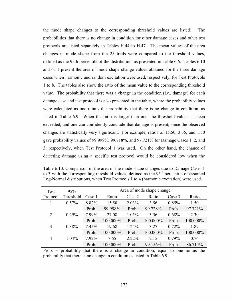
172
the mode shape changes to the corresponding threshold values are listed). The
probabilities that there is no change in condition for other damage cases and other test
protocols are listed separately in Tables H.44 to H.47. The mean values of the area
changes in mode shape from the 25 trials were compared to the threshold values,
defined as the 95th percentile of the distribution, as presented in Table 6.6. Tables 6.10
and 6.11 present the area of mode shape change values obtained for the three damage
cases when harmonic and random excitation were used, respectively, for Test Protocols
1 to 8. The tables also show the ratio of the mean value to the corresponding threshold
value. The probability that there was a change in the condition (i.e., damage) for each
damage case and test protocol is also presented in the table, where the probability values
were calculated as one minus the probability that there is no change in condition, as
listed in Table 6.9. When the ratio is larger than one, the threshold value has been
exceeded, and one can confidently conclude that damage is present, since the observed
changes are statistically very significant. For example, ratios of 15.50, 3.35, and 1.50
gave probability values of 99.998%, 99.718%, and 97.721% for Damage Cases 1, 2, and
3, respectively, when Test Protocol 1 was used. On the other hand, the chance of
detecting damage using a specific test protocol would be considered low when the
Table 6.10. Comparison of the area of the mode shape changes due to Damage Cases 1 to 3 with the corresponding threshold values, defined as the 95th percentile of assumed Log-Normal distributions, when Test Protocols 1 to 4 (harmonic excitation) were used.
Test Protocol
95% Threshold
Area of mode shape change
Case 1 Ratio Case 2 Ratio Case 3 Ratio 1 0.57% 8.82% 15.50 2.03% 3.56 0.85% 1.50
Prob. 99.998% Prob. 99.728% Prob. 97.721% 2 0.29% 7.99% 27.08 1.05% 3.56 0.68% 2.30
Prob. 100.000% Prob. 100.000% Prob. 100.000% 3 0.38% 7.45% 19.68 1.24% 3.27 0.72% 1.89
Prob. 100.000% Prob. 100.000% Prob. 100.000% 4 1.04% 7.92% 7.65 2.22% 2.15 0.79% 0.76 Prob. 100.000% Prob. 99.156% Prob. 86.714%
Prob. = probability that there is a change in condition, equal to one minus the probability that there is no change in condition as listed in Table 6.9.
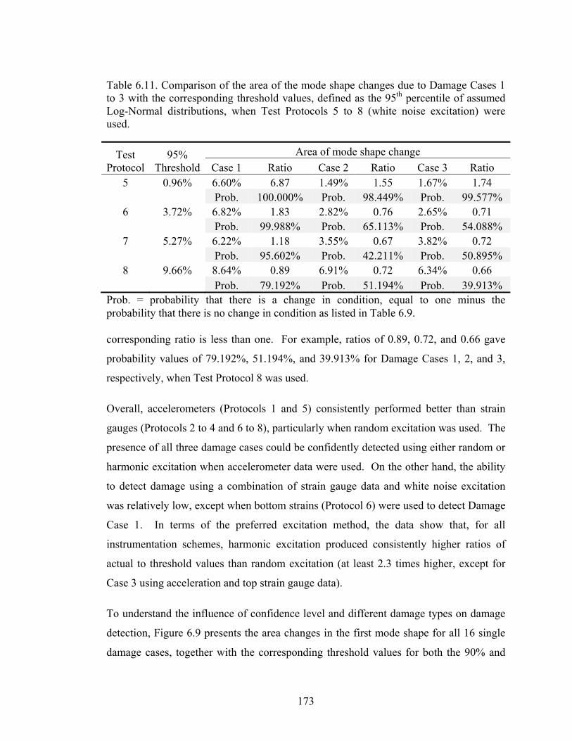
173
corresponding ratio is less than one. For example, ratios of 0.89, 0.72, and 0.66 gave
probability values of 79.192%, 51.194%, and 39.913% for Damage Cases 1, 2, and 3,
respectively, when Test Protocol 8 was used.
Overall, accelerometers (Protocols 1 and 5) consistently performed better than strain
gauges (Protocols 2 to 4 and 6 to 8), particularly when random excitation was used. The
presence of all three damage cases could be confidently detected using either random or
harmonic excitation when accelerometer data were used. On the other hand, the ability
to detect damage using a combination of strain gauge data and white noise excitation
was relatively low, except when bottom strains (Protocol 6) were used to detect Damage
Case 1. In terms of the preferred excitation method, the data show that, for all
instrumentation schemes, harmonic excitation produced consistently higher ratios of
actual to threshold values than random excitation (at least 2.3 times higher, except for
Case 3 using acceleration and top strain gauge data).
To understand the influence of confidence level and different damage types on damage
detection, Figure 6.9 presents the area changes in the first mode shape for all 16 single
damage cases, together with the corresponding threshold values for both the 90% and
Table 6.11. Comparison of the area of the mode shape changes due to Damage Cases 1 to 3 with the corresponding threshold values, defined as the 95th percentile of assumed Log-Normal distributions, when Test Protocols 5 to 8 (white noise excitation) were used.
Test Protocol
95% Threshold
Area of mode shape change
Case 1 Ratio Case 2 Ratio Case 3 Ratio 5 0.96% 6.60% 6.87 1.49% 1.55 1.67% 1.74
Prob. 100.000% Prob. 98.449% Prob. 99.577% 6 3.72% 6.82% 1.83 2.82% 0.76 2.65% 0.71
Prob. 99.988% Prob. 65.113% Prob. 54.088% 7 5.27% 6.22% 1.18 3.55% 0.67 3.82% 0.72
Prob. 95.602% Prob. 42.211% Prob. 50.895% 8 9.66% 8.64% 0.89 6.91% 0.72 6.34% 0.66 Prob. 79.192% Prob. 51.194% Prob. 39.913%
Prob. = probability that there is a change in condition, equal to one minus the probability that there is no change in condition as listed in Table 6.9.
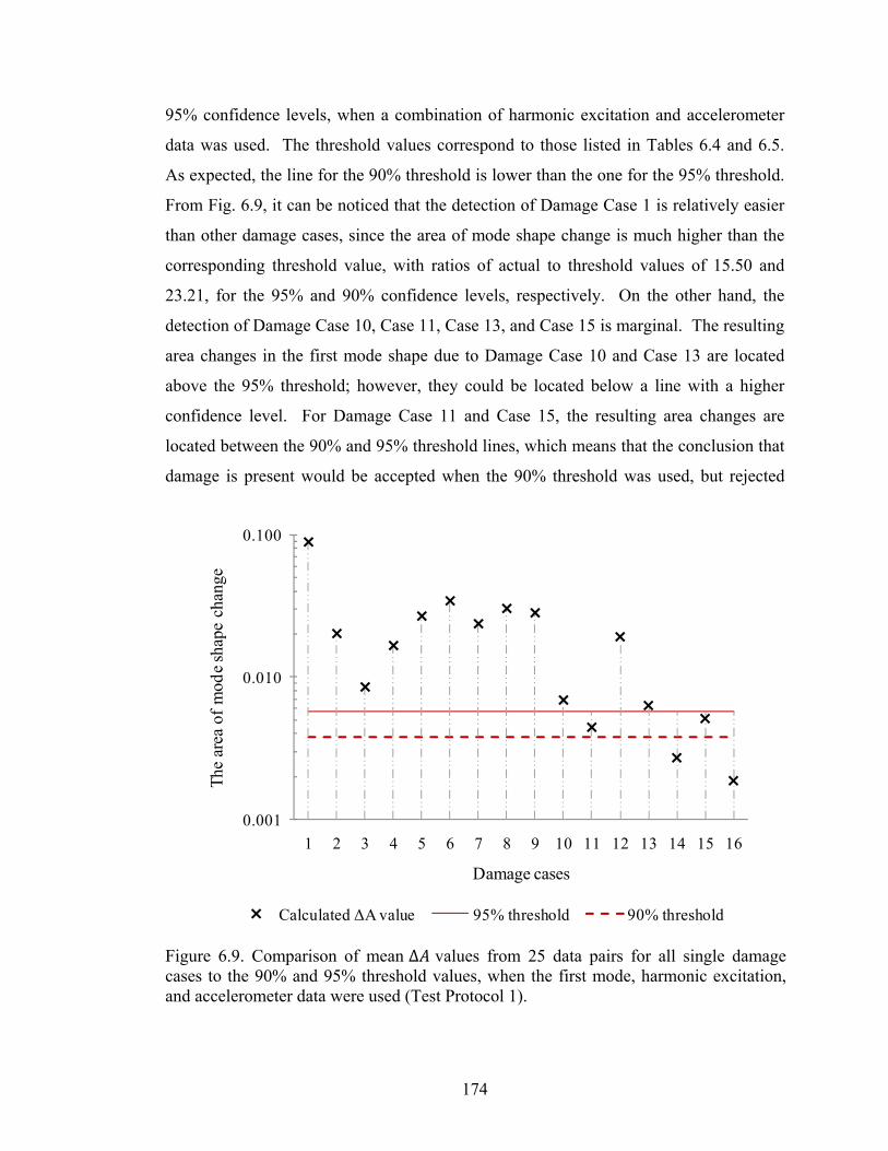
174
95% confidence levels, when a combination of harmonic excitation and accelerometer
data was used. The threshold values correspond to those listed in Tables 6.4 and 6.5.
As expected, the line for the 90% threshold is lower than the one for the 95% threshold.
From Fig. 6.9, it can be noticed that the detection of Damage Case 1 is relatively easier
than other damage cases, since the area of mode shape change is much higher than the
corresponding threshold value, with ratios of actual to threshold values of 15.50 and
23.21, for the 95% and 90% confidence levels, respectively. On the other hand, the
detection of Damage Case 10, Case 11, Case 13, and Case 15 is marginal. The resulting
area changes in the first mode shape due to Damage Case 10 and Case 13 are located
above the 95% threshold; however, they could be located below a line with a higher
confidence level. For Damage Case 11 and Case 15, the resulting area changes are
located between the 90% and 95% threshold lines, which means that the conclusion that
damage is present would be accepted when the 90% threshold was used, but rejected
Figure 6.9. Comparison of mean Δ values from 25 data pairs for all single damagecases to the 90% and 95% threshold values, when the first mode, harmonic excitation,and accelerometer data were used (Test Protocol 1).
0.001
0.010
0.100
1 2 3 4 5 6 7 8 9 10 11 12 13 14 15 16
The
are
a of
mod
e sh
ape
chan
ge
Damage cases
Calculated ΔA value 95% threshold 90% threshold

175
when the 95% threshold was used. For Damage Case 14 and Case 16, there would be
little chance of detecting damage since the resulting area changes are located
considerably below both threshold lines. Results for other sensor schemes and
excitation types are available in Appendix H.
6.2.7 Influence of sensor scheme on the performance of the damage indicator
To ascertain the influence of the sensor scheme on the performance of the area of mode
shape change damage indicator, the ratios of Δ values (using the average values of 25
trials) to the 95% threshold values were calculated for all damage cases and all sensor
schemes. The resulting ratios were then plotted, with all sensor schemes and damage
cases shown on a single plot. Since ratios are used, the threshold values (or relative
threshold value) are equal to one for all test protocols.
Figure 6.10 presents the results for the first mode when harmonic excitation was used
(Test Protocols 1 to 4). As previously described, the likelihood that the condition of the
bridge has not changed is considered too high to conclude the presence of the damage
when the values of area change fall below the threshold line. On the other hand, if a
change in area above the threshold line is observed, the chance that the condition of the
structure is unchanged is sufficiently small (less than 5%) so as to conclude that a
change in health condition (i.e., damage) has indeed occurred, since the area change is
statistically significant. From Fig. 6.10, it can be clearly noticed that all sensor schemes,
except for the one that used the top strain gauges, showed similar performance for
damage detection when the fundamental mode shape and harmonic excitation were
used. This means that the low cost strain gauges are capable of generating mode shapes
of sufficient quality for damage detection, as long as they are properly positioned and
the excitation forces are strong enough to produce strain readings with high signal to
noise ratios. Generally, the presence of damage for damage cases involving the steel
girder (Case 1), the diaphragms (Cases 2 through 7), and the steel straps (Cases 8
through 11) could be detected using all sensor schemes, except for several cases when
the top strain gauges were used in conjunction with Damage Case 11. The chance of
detecting the presence of the damage to the concrete deck (Cases 12-16) was relatively

176
small no matter which sensor scheme was selected, which is similar to the results found
for simulated damage to the concrete deck, as described in Chapter 5.
When white noise excitation was used in combination with the first mode, as presented
in Fig. 6.11, the use of accelerometers was clearly superior to all other sensor schemes.
The use of accelerometer data allowed the detection of all damage cases to the steel
girder, diaphragms, and steel straps except for Damage Case 7 (D-X2.8Y1.35) and Case
10 (ST-X4.4Y1.35). None of the strain gauge schemes were capable of detecting the
presence of any of the damage cases, except for Damage Case 1, since the area changes
were not statistically significant. For damage category 4 (i.e., damage to the concrete
Figure 6.10. Ratios of area of mode shape change (the average of 25 values) to the 95%threshold values for all sensor schemes and damage cases, when the first mode andharmonic excitation were used (Test Protocols 1 to 4).
0.1
1
10
100
1 2 3 4 5 6 7 8 9 10 11 12 13 14 15 16
Rat
ios
of a
rea
of m
ode
shap
e ch
ange
Damage cases
Accelerometer Bottom strain Middle strain
Top strain 95% threshold
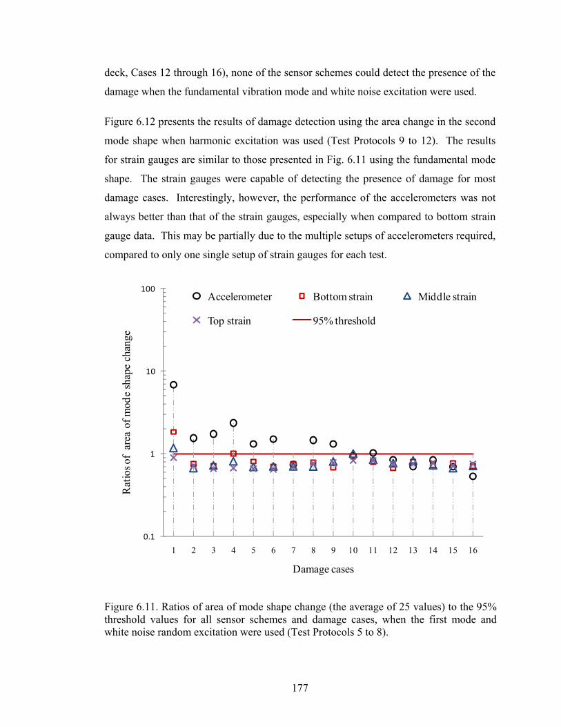
177
deck, Cases 12 through 16), none of the sensor schemes could detect the presence of the
damage when the fundamental vibration mode and white noise excitation were used.
Figure 6.12 presents the results of damage detection using the area change in the second
mode shape when harmonic excitation was used (Test Protocols 9 to 12). The results
for strain gauges are similar to those presented in Fig. 6.11 using the fundamental mode
shape. The strain gauges were capable of detecting the presence of damage for most
damage cases. Interestingly, however, the performance of the accelerometers was not
always better than that of the strain gauges, especially when compared to bottom strain
gauge data. This may be partially due to the multiple setups of accelerometers required,
compared to only one single setup of strain gauges for each test.
Figure 6.11. Ratios of area of mode shape change (the average of 25 values) to the 95%threshold values for all sensor schemes and damage cases, when the first mode andwhite noise random excitation were used (Test Protocols 5 to 8).
0.1
1
10
100
1 2 3 4 5 6 7 8 9 10 11 12 13 14 15 16
Rat
ios
of a
rea
of m
ode
shap
e ch
ange
Damage cases
Accelerometer Bottom strain Middle strain
Top strain 95% threshold
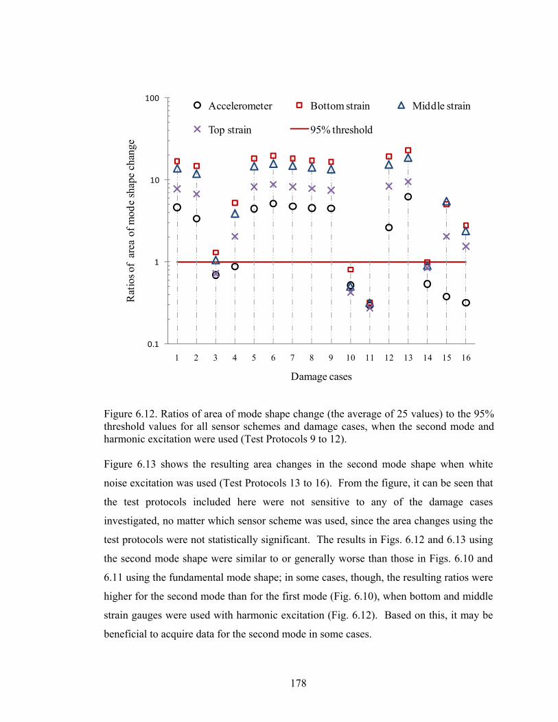
178
Figure 6.13 shows the resulting area changes in the second mode shape when white
noise excitation was used (Test Protocols 13 to 16). From the figure, it can be seen that
the test protocols included here were not sensitive to any of the damage cases
investigated, no matter which sensor scheme was used, since the area changes using the
test protocols were not statistically significant. The results in Figs. 6.12 and 6.13 using
the second mode shape were similar to or generally worse than those in Figs. 6.10 and
6.11 using the fundamental mode shape; in some cases, though, the resulting ratios were
higher for the second mode than for the first mode (Fig. 6.10), when bottom and middle
strain gauges were used with harmonic excitation (Fig. 6.12). Based on this, it may be
beneficial to acquire data for the second mode in some cases.
Figure 6.12. Ratios of area of mode shape change (the average of 25 values) to the 95%threshold values for all sensor schemes and damage cases, when the second mode andharmonic excitation were used (Test Protocols 9 to 12).
0.1
1
10
100
1 2 3 4 5 6 7 8 9 10 11 12 13 14 15 16
Rat
ios
of a
rea
of m
ode
shap
e ch
ange
Damage cases
Accelerometer Bottom strain Middle strain
Top strain 95% threshold
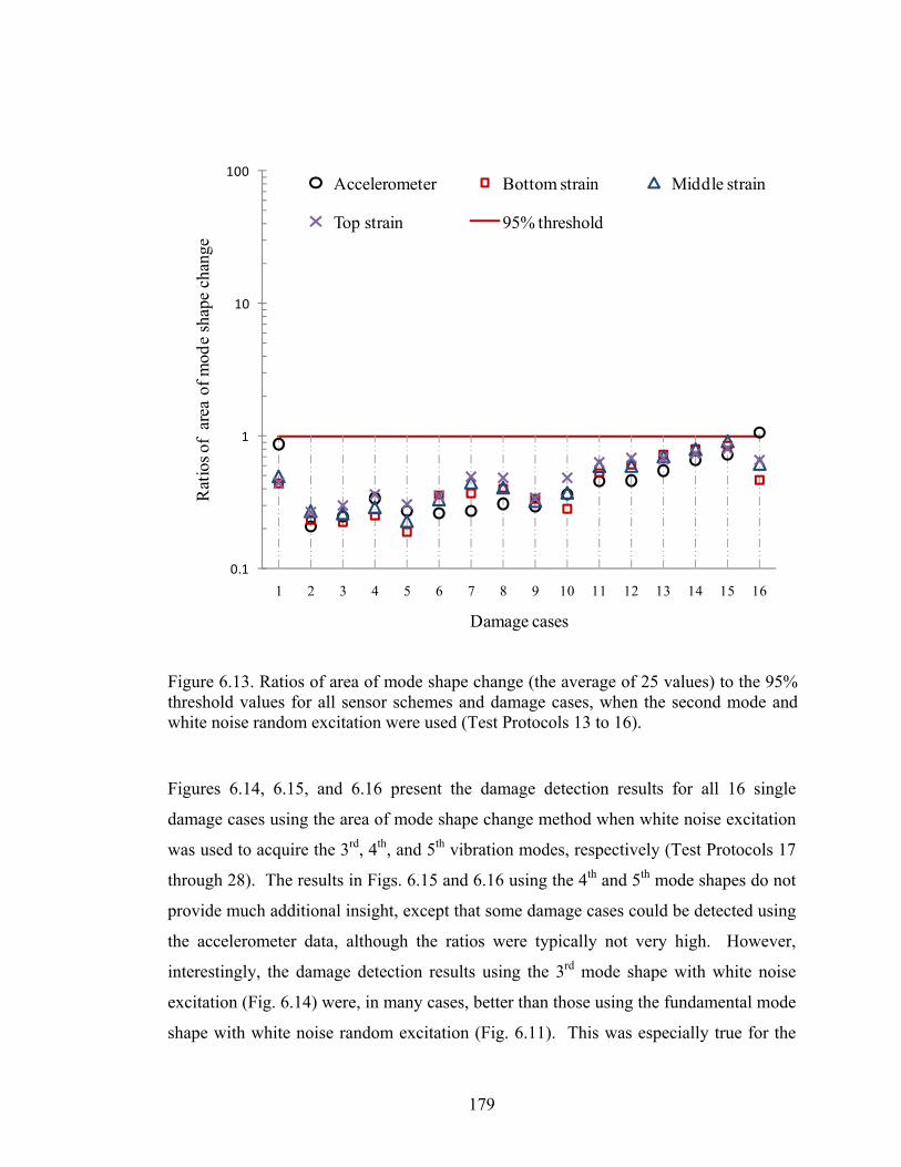
179
Figures 6.14, 6.15, and 6.16 present the damage detection results for all 16 single
damage cases using the area of mode shape change method when white noise excitation
was used to acquire the 3rd, 4th, and 5th vibration modes, respectively (Test Protocols 17
through 28). The results in Figs. 6.15 and 6.16 using the 4th and 5th mode shapes do not
provide much additional insight, except that some damage cases could be detected using
the accelerometer data, although the ratios were typically not very high. However,
interestingly, the damage detection results using the 3rd mode shape with white noise
excitation (Fig. 6.14) were, in many cases, better than those using the fundamental mode
shape with white noise random excitation (Fig. 6.11). This was especially true for the
Figure 6.13. Ratios of area of mode shape change (the average of 25 values) to the 95%threshold values for all sensor schemes and damage cases, when the second mode andwhite noise random excitation were used (Test Protocols 13 to 16).
0.1
1
10
100
1 2 3 4 5 6 7 8 9 10 11 12 13 14 15 16
Rat
ios
of a
rea
of m
ode
shap
e ch
ange
Damage cases
Accelerometer Bottom strain Middle strain
Top strain 95% threshold

180
damage cases which could produce the greatest changes in global load sharing (i.e., the
damage to diaphragms and steel straps, which included Cases 2 through 11), even
though the threshold values for all sensor schemes using the 3rd mode were much higher
than those using the fundamental mode. In fact, the threshold values for the 3rd mode
were at least 2.79 times higher, which means that the test protocols using the 3rd mode
should be much less sensitive to damage than those using the fundamental mode. The
reason for this may be explained by the fact that the combined flexural and torsional 3rd
mode shape transformed to a new mode (or a mode which was very different from the
one before the damage was introduced) due to the introduction of damage that changed
the global stiffness distribution of the structure (for example, see Fig. E.4 in Appendix E,
for a comparison of the third mode shape before and after Damage Case 2 or Health
Figure 6.14. Ratios of area of mode shape change (the average of 25 values) to the 95%threshold values for all sensor schemes and damage cases, when the third mode andwhite noise random excitation were used (Test Protocols 17 to 20).
0.1
1
10
100
1 2 3 4 5 6 7 8 9 10 11 12 13 14 15 16
Rat
ios
of a
rea
of m
ode
shap
e ch
ange
Damage cases
Accelerometer Bottom strain Middle strain
Top strain 95% threshold
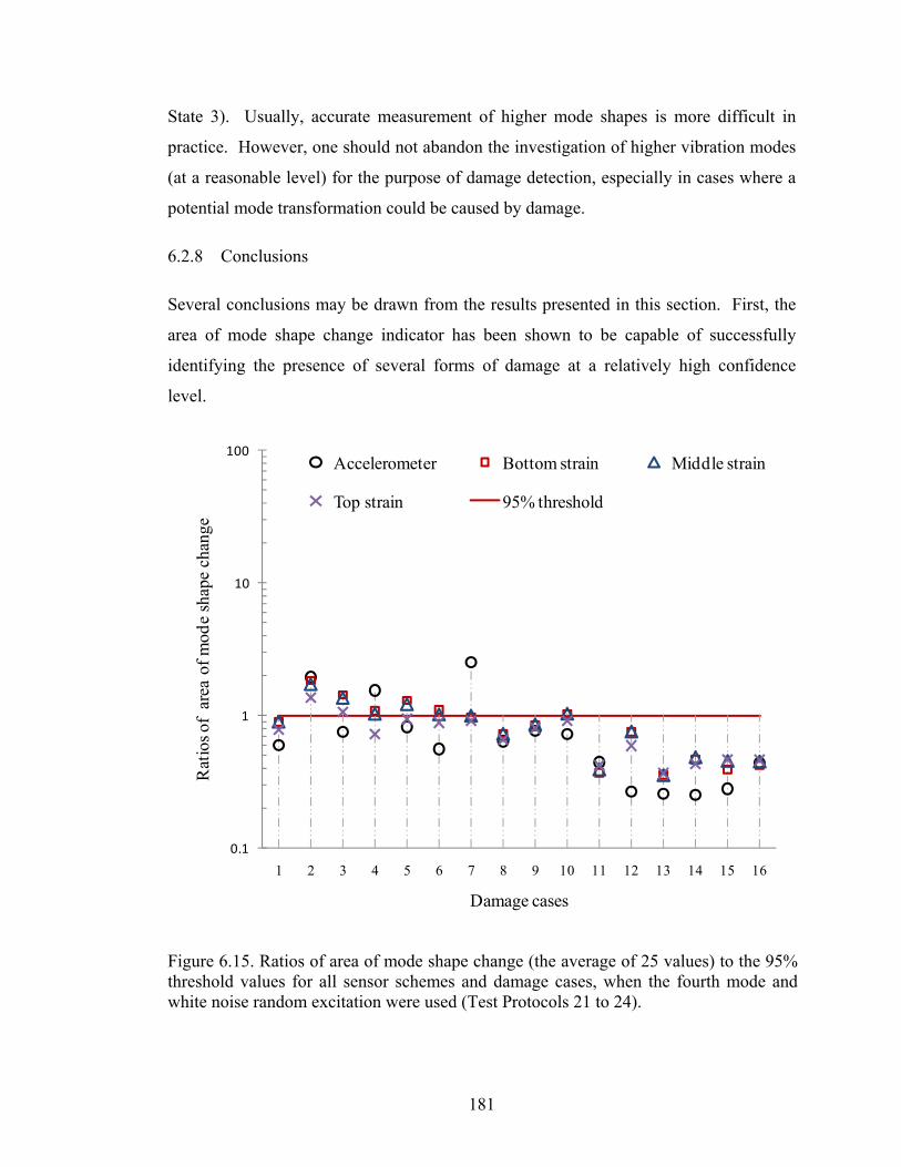
181
State 3). Usually, accurate measurement of higher mode shapes is more difficult in
practice. However, one should not abandon the investigation of higher vibration modes
(at a reasonable level) for the purpose of damage detection, especially in cases where a
potential mode transformation could be caused by damage.
6.2.8 Conclusions
Several conclusions may be drawn from the results presented in this section. First, the
area of mode shape change indicator has been shown to be capable of successfully
identifying the presence of several forms of damage at a relatively high confidence
level.
Figure 6.15. Ratios of area of mode shape change (the average of 25 values) to the 95%threshold values for all sensor schemes and damage cases, when the fourth mode andwhite noise random excitation were used (Test Protocols 21 to 24).
0.1
1
10
100
1 2 3 4 5 6 7 8 9 10 11 12 13 14 15 16
Rat
ios
of a
rea
of m
ode
shap
e ch
ange
Damage cases
Accelerometer Bottom strain Middle strain
Top strain 95% threshold
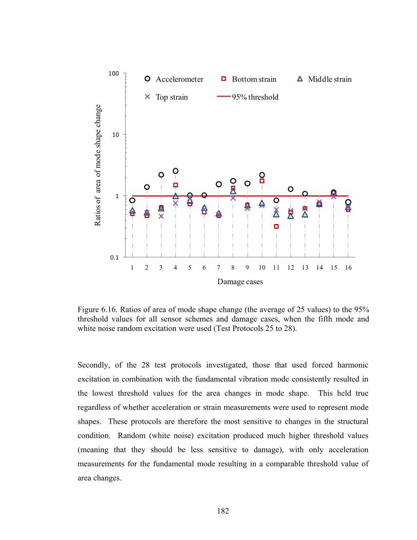
182
Secondly, of the 28 test protocols investigated, those that used forced harmonic
excitation in combination with the fundamental vibration mode consistently resulted in
the lowest threshold values for the area changes in mode shape. This held true
regardless of whether acceleration or strain measurements were used to represent mode
shapes. These protocols are therefore the most sensitive to changes in the structural
condition. Random (white noise) excitation produced much higher threshold values
(meaning that they should be less sensitive to damage), with only acceleration
measurements for the fundamental mode resulting in a comparable threshold value of
area changes.
Figure 6.16. Ratios of area of mode shape change (the average of 25 values) to the 95%threshold values for all sensor schemes and damage cases, when the fifth mode andwhite noise random excitation were used (Test Protocols 25 to 28).
0.1
1
10
100
1 2 3 4 5 6 7 8 9 10 11 12 13 14 15 16
Rat
ios
of a
rea
of m
ode
shap
e ch
ange
Damage cases
Accelerometer Bottom strain Middle strain
Top strain 95% threshold
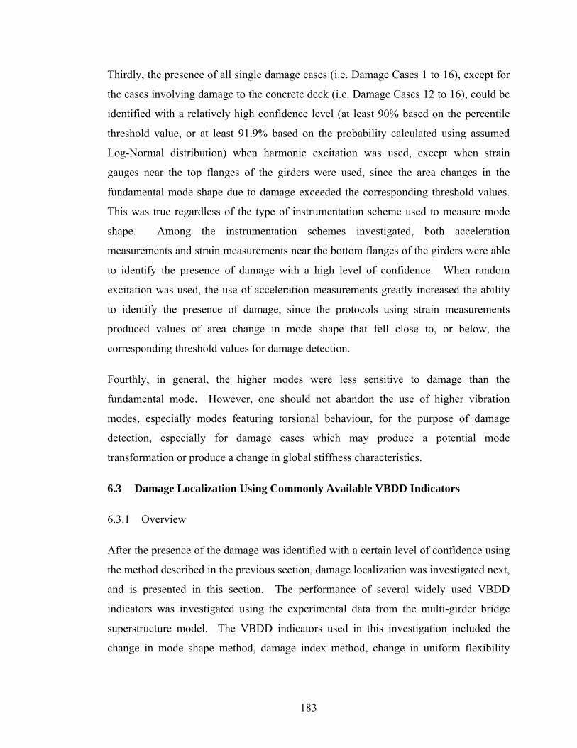
183
Thirdly, the presence of all single damage cases (i.e. Damage Cases 1 to 16), except for
the cases involving damage to the concrete deck (i.e. Damage Cases 12 to 16), could be
identified with a relatively high confidence level (at least 90% based on the percentile
threshold value, or at least 91.9% based on the probability calculated using assumed
Log-Normal distribution) when harmonic excitation was used, except when strain
gauges near the top flanges of the girders were used, since the area changes in the
fundamental mode shape due to damage exceeded the corresponding threshold values.
This was true regardless of the type of instrumentation scheme used to measure mode
shape. Among the instrumentation schemes investigated, both acceleration
measurements and strain measurements near the bottom flanges of the girders were able
to identify the presence of damage with a high level of confidence. When random
excitation was used, the use of acceleration measurements greatly increased the ability
to identify the presence of damage, since the protocols using strain measurements
produced values of area change in mode shape that fell close to, or below, the
corresponding threshold values for damage detection.
Fourthly, in general, the higher modes were less sensitive to damage than the
fundamental mode. However, one should not abandon the use of higher vibration
modes, especially modes featuring torsional behaviour, for the purpose of damage
detection, especially for damage cases which may produce a potential mode
transformation or produce a change in global stiffness characteristics.
6.3 Damage Localization Using Commonly Available VBDD Indicators
6.3.1 Overview
After the presence of the damage was identified with a certain level of confidence using
the method described in the previous section, damage localization was investigated next,
and is presented in this section. The performance of several widely used VBDD
indicators was investigated using the experimental data from the multi-girder bridge
superstructure model. The VBDD indicators used in this investigation included the
change in mode shape method, damage index method, change in uniform flexibility

184
curvature method, change in flexibility method, and change in mode shape curvature
method. These methods are described in Section 2.5.
To ensure that mode shapes were scaled to a common basis, the mode shapes used in
this investigation were first normalized by the unit-area normalization method as
described in Section 4.4.3. Prior to normalization, modal amplitudes between the
measurement points were interpolated using the natural cubic spline interpolation
method (see Section 4.4.3) to produce mode shapes that were defined at 49 points along
each girder line. For each individual health (or damage) condition, five repeated trials
were conducted for each vibration mode. Then, the average mode shapes calculated
from the five trials for both undamaged and damaged conditions were used to apply the
damage detection equations described in Section 2.5.
Of the 28 test protocols included in this research, only the most sensitive one -- the
fundamental mode shape extracted using the accelerometer data with the harmonic
excitation -- was selected and investigated in this section. To demonstrate the method,
only Damage Case 1, for which the bottom plate was removed from the splice at mid-
span of Girder 4 (see Table 3.5), was investigated in detail. Results related to damage
localization for other damage cases using other test protocols are available in Appendix
I, Appendix J, and Appendix K.
Figure 6.17 to Figure 6.21 show the distributions of the selected VBDD indicators for
this damage case. The circle in the figures indicates the actual location of damage. In
these distributions, the highest peak(s) in the graph corresponds to the likely
longitudinal location(s) of damage. It can be seen from the figures that, in general, all
methods produced a peak at the damage location, although in most cases it was the
second highest peak. Therefore, as long as one was able to establish the presence of
damage with a certain level of confidence, these results would limit the possible
locations of damage to a relatively small number. A detailed discussion of the results
for each VBDD indictor is available in the following sections.

185
6.3.2 Change in mode shape method
Changes in the fundamental mode shape due to Damage Case 1 are illustrated in Fig.
6.17, both in 2D form showing plots along individual girder lines and in 3D form
showing the entire deck surface. In parts (a) and (b) of this figure, the mode shapes
have been normalized using all measurement and interpolated points; thus, a total of 196
points were used for the normalization, 49 points for each girder. These figures
therefore show the global shape of the change in mode. In part (c), on the other hand,
the mode shapes have been normalized separately along each individual girder line (see
Section 4.4.4), resulting in a different mode shape scaling factor for each girder line; this
approach shows the localized shape of the changes along each girder.
Considering the normalization scheme over all measurement points (Figs. 6.17(a) and
(b)), mode shape changes were found to be broadly distributed, producing smooth mode
shape change plots along all girder lines. Also, the mode shape change patterns for this
damage case are nearly symmetric about the longitudinal centreline of the deck. Since
the largest positive peak in the change in mode shape plots coincides with the actual
location of damage at mid-span of Girder 4, damage localization may be deemed to be
successful in this case, in both the longitudinal and transverse directions. However,
further investigations need to be conducted to draw concrete conclusions about the
damage localization ability in the transverse direction. Furthermore, the presence of
damage could be detected using measurements at any location on the deck due to the
wide dispersion of the mode shape change.
When the mode shapes were normalized separately along individual girder lines (Fig.
6.17(c)), the change in mode shape patterns was altered significantly. In this case, the
positive peak at the damage location along Girder Line 4 is more clearly defined,
making damage localization more precise. However, a larger positive peak also exists
along Girder Line 1, introducing the possibility of a spurious diagnosis of damage at
that location. This spurious diagnosis is common for multiple girder systems, even in
numerical studies (Siddique 2008). In addition, the amplitudes of mode shape changes
along Girder lines 2 and 3 were relatively small, suggesting that damage detection using

186
-0.03
-0.02
-0.01
0.00
0.01
0.02
0.03
0.04
0.05
0 1 2 3 4 5 6 7 8
Cha
nge
in m
ode
shap
e
Longitudinal distance from the left support (m)
Girder line 1 Girder line 2
Girder line 3 Girder line 4
Actual damage location
-0.30
-0.20
-0.10
0.00
0.10
0.20
0.30
0 1 2 3 4 5 6 7 8
Cha
nge
in m
ode
shap
e
Longitudinal distance from the left support (m)
00.9
1.82.7
-0.3
-0.2
-0.1
0
0.1
0.2
0.3
0 1 2 3 4 5 6 7 8
Cha
nge
in m
ode
shap
e
Figure 6.17. Distribution of the change in the first mode shape due to Damage Case 1using accelerometer data with harmonic excitation: (a) 3D figure with unit areanormalization over all measurement points; (b) 2D figure with unit area normalizationover all measurement points; and (c) 2D figure with unit area normalization alongindividual girder lines.
(a)
(c)
(b)
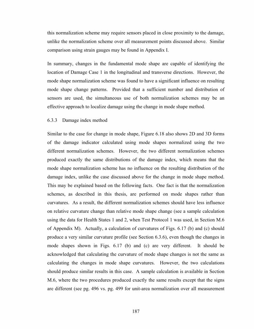
187
this normalization scheme may require sensors placed in close proximity to the damage,
unlike the normalization scheme over all measurement points discussed above. Similar
comparison using strain gauges may be found in Appendix I.
In summary, changes in the fundamental mode shape are capable of identifying the
location of Damage Case 1 in the longitudinal and transverse directions. However, the
mode shape normalization scheme was found to have a significant influence on resulting
mode shape change patterns. Provided that a sufficient number and distribution of
sensors are used, the simultaneous use of both normalization schemes may be an
effective approach to localize damage using the change in mode shape method.
6.3.3 Damage index method
Similar to the case for change in mode shape, Figure 6.18 also shows 2D and 3D forms
of the damage indicator calculated using mode shapes normalized using the two
different normalization schemes. However, the two different normalization schemes
produced exactly the same distributions of the damage index, which means that the
mode shape normalization scheme has no influence on the resulting distribution of the
damage index, unlike the case discussed above for the change in mode shape method.
This may be explained based on the following facts. One fact is that the normalization
schemes, as described in this thesis, are performed on mode shapes rather than
curvatures. As a result, the different normalization schemes should have less influence
on relative curvature change than relative mode shape change (see a sample calculation
using the data for Health States 1 and 2, when Test Protocol 1 was used, in Section M.6
of Appendix M). Actually, a calculation of curvatures of Figs. 6.17 (b) and (c) should
produce a very similar curvature profile (see Section 6.3.6), even though the changes in
mode shapes shown in Figs. 6.17 (b) and (c) are very different. It should be
acknowledged that calculating the curvature of mode shape changes is not the same as
calculating the changes in mode shape curvatures. However, the two calculations
should produce similar results in this case. A sample calculation is available in Section
M.6, where the two procedures produced exactly the same results except that the signs
are different (see pg. 496 vs. pg. 499 for unit-area normalization over all measurement

188
points and pg. 497 vs. pg. 500 for unit-area normalization along individual girder lines).
The sign difference is due to the fact that the changes in mode shape curvatures were
calculated using absolute values, as described in Section 2.5.6. Since the damage index
is a function of mode shape curvature, the normalization schemes should have less
influence on the values of damage index. Furthermore, the damage index used in this
calculation was normalized (or scaled) to a standard normal distribution (see Eq. 2.8),
which produced exactly the same amplitudes and shape of the damage index for the two
different normalization schemes. As a result, the two different mode shape
normalization schemes produced exactly the same damage index profile. Similar results
were found in numerical studies on a multiple girder system (see Fig. 7.6 in Siddique
2008).
Since the largest positive peak in the damage index plots coincides with the actual
location of damage at mid-span of Girder 4, one can conclude that the damage location
could be successfully located. In addition, the narrow range of the positive peak at the
damage location gives a clear indication of the location of damage, which makes
damage localization relatively precise. However, the relatively large peak in the
damage index at the quarter span of the other three girders may lead to some ambiguity
regarding where the damage might actually be located.
6.3.4 Change in uniform flexibility curvature method
Figure 6.19 presents the distribution of change in uniform flexibility curvature for the
first mode shape due to Damage Case 1 using accelerometer data with harmonic
excitation. Once again, parts (a) and (b) of this figure show the results when the mode
shapes were normalized using all measurement points, while part (c) represents the
results when mode shapes were normalized separately along individual girder lines.
Comparing parts (b) and (c), it can seen that the two normalization schemes produced
similar results, except that normalization along individual girder lines (part c) generated
relatively flatter curves near the supports. As described above, since the normalization
is performed on mode shapes rather than curvatures, the relative curvature relationship
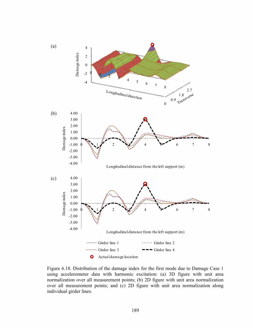
189
-4.00
-3.00
-2.00
-1.00
0.00
1.00
2.00
3.00
4.00
0 1 2 3 4 5 6 7 8
Dam
age
inde
x
Longitudinal distance from the left support (m)
Girder line 1 Girder line 2
Girder line 3 Girder line 4
Actual damage location
-4.00
-3.00
-2.00
-1.00
0.00
1.00
2.00
3.00
4.00
0 1 2 3 4 5 6 7 8
Dam
age
inde
x
Longitudinal distance from the left support (m)
00.9
1.82.7
-4
-2
0
2
4
0 1 2 3 4 5 6 7 8
Dam
age
inde
x
Figure 6.18. Distribution of the damage index for the first mode due to Damage Case 1using accelerometer data with harmonic excitation: (a) 3D figure with unit areanormalization over all measurement points; (b) 2D figure with unit area normalizationover all measurement points; and (c) 2D figure with unit area normalization alongindividual girder lines.
(a)
(c)
(b)

190
-400.00-300.00-200.00-100.00
0.00100.00200.00300.00400.00500.00600.00
0 2 4 6 8
Cha
nge
in u
nifo
rm fl
exib
ility
curv
atur
e
Longitudinal distance from the left support (m)
Girder line 1 Girder line 2
Girder line 3 Girder line 4
Actual damage location
-800.00
-600.00
-400.00
-200.00
0.00
200.00
400.00
600.00
0 1 2 3 4 5 6 7 8
Cha
nge
in u
nifo
rm
flex
ibili
ty c
urva
ture
Longitudinal distance from the left support (m)
0
1.8
-800-600-400-200
0200400600
0 1 2 3 4 5 6 7 8
Cha
nge
in u
nifo
rm fl
exib
ility
cu
rvat
ure
Figure 6.19. Distribution of the change in uniform flexibility curvature for the first modedue to Damage Case 1 using accelerometer data with harmonic excitation: (a) 3D figurewith unit area normalization over all measurement points; (b) 2D figure with unit areanormalization over all measurement points; and (c) 2D figure with unit areanormalization along individual girder lines.
(a)
(c)
(b)

191
between compared pairs is not changed significantly. As a result, the normalization
schemes should have less influence on relative curvature change.
For both normalization schemes, the second largest peak coincided with the actual
damage location, implying that this method is capable of locating the damage, or at least
limiting the possible location of damage to two locations. The largest peak corresponds
to a false indicator, as stated above.
6.3.5 Change in flexibility method
Figure 6.20 presents the results using the change in flexibility method, which is similar
to those of the change in mode shape method (Fig. 6.17).
When normalization over all measurement points was used (Figs. 6.20(a) and (b)), the
change in flexibility was found to be broadly distributed, producing smooth plots along
all girder lines. Similar to the previous description for change in mode shape, the
change in flexibility patterns for this damage case are nearly symmetric about the
longitudinal centreline of the deck. Unlike the case for the change in mode shape
method, the largest positive peak in the change in flexibility plots occurred close to the
mid-span of Girder 1, which would be a false positive indicator. However, the second
highest peak coincided with the actual location of the damage; this can be deemed to be
a successful damage localization in the sense that the possible location of damage was
limited to two locations.
For the case using normalization along individual girder lines, as shown in Fig. 6.20(c),
the results were very similar to those of the change in mode shape method. The second
highest positive peak coincided with the actual damage location, while the highest
positive peak may correspond to a false indicator. As a result, one can claim that the
damage indicator is capable of identifying the location of damage although not without
some possible ambiguity.

192
0.00
0.02
0.04
0.06
0.08
0.10
0 1 2 3 4 5 6 7 8
Cha
nge
in fl
exib
ility
Longitudinal distance from the left support (m)
Girder line 1 Girder line 2
Girder line 3 Girder line 4
Actual damage location
0.00
0.20
0.40
0.60
0.80
0 1 2 3 4 5 6 7 8
Cha
nge
in fl
exib
ility
Longitudinal distance from the left support (m)
00.9
1.82.7
0
0.2
0.4
0.6
0.8
0 1 2 3 4 5 6 7 8
Cha
nge
in fl
exib
ility
Figure 6.20. Distribution of the change in flexibility for the first mode due to DamageCase 1 using accelerometer data with harmonic excitation: (a) 3D figure with unit areanormalization over all measurement points; (b) 2D figure with unit area normalizationover all measurement points; and (c) 2D figure with unit area normalization alongindividual girder lines.
(a)
(c)
(b)

193
6.3.6 Change in mode shape curvature method
The damage localization results for Damage Case 1 using the change in mode shape
curvature method are presented in Fig. 6.21. The results shown in this figure are very
similar to those in Fig. 6.19, except for the differences in the amplitude of changes. As
a result, the description and conclusions for change in uniform flexibility curvature
method (Section 6.3.4) also apply to the change in mode shape curvature.
The change in mode shape curvature method investigated is capable of identifying the
location of damage after the presence of damage has been established, as described in
Section 6.2. In addition, the normalization schemes appear to have little influence on
the damage localization results when this VBDD method is used, as described in Section
6.3.3.

194
-15.00
-10.00
-5.00
0.00
5.00
10.00
15.00
0 1 2 3 4 5 6 7 8
Cha
nge
in m
ode
shap
e cu
rvat
ure
Longitudinal distance from the left support (m)
00.9
1.82.7
-15
-10
-5
0
5
10
15
0 1 2 3 4 5 6 7 8
Cha
nge
in m
ode
shap
ecu
rvat
ure
-10.00
-5.00
0.00
5.00
10.00
15.00
0 1 2 3 4 5 6 7 8
Cha
nge
in m
ode
shap
e cu
rvat
ure
Longitudinal distance from the left support (m)
Girder line 1 Girder line 2
Girder line 3 Girder line 4
Actual damage location
Figure 6.21. Distribution of the change in mode shape curvature for the first mode dueto Damage Case 1 using accelerometer data with harmonic excitation: (a) 3D figure withunit area normalization over all measurement points; (b) 2D figure with unit areanormalization over all measurement points; and (c) 2D figure with unit areanormalization along individual girder lines.
(a)
(c)
(b)
195
CHAPTER 7. SUMMARY AND CONCLUSIONS
7.1 Summary
This thesis investigated a number of issues related to the potential use of vibration-based
damage detection (VBDD) methods for the structural health monitoring (SHM) of
bridge superstructures using both experimental and numerical studies. The primary
objective of this research was to investigate the application of VBDD methods to multi-
girder bridge superstructures.
The research focused primarily on an experimental investigation of VBDD on a multi-
girder bridge superstructure, while theoretical analyses and numerical verifications were
also included. The structure used for this investigation was a one-third scale model of a
slab-on-girder composite bridge superstructure featuring four steel girders supporting a
steel-free concrete deck.
The experimental tests were conducted under well-controlled environments. Forced
dynamic excitation was supplied by means of a feedback-controlled hydraulic shaker.
Instrumentation used to measure the dynamic response included a closely-spaced grid of
accelerometers mounted on the surface of the deck along the girder lines, as well as
electrical-resistance foil strain gauges bonded to the girder webs.
Measurement of the modal properties of the multi-girder bridge superstructure was
carried out in two phases. In Phase I, the influence of various test parameters on the
repeatability and reliability of modal property extraction was investigated using the
intact bridge model. More specifically, the test parameters that were considered in the
intact bridge model tests included sampling rates, the length of the recording period,
excitation methods, sensor type, and sensor locations (i.e., the vertical locations of strain
196
gauges on the steel web). For the tests conducted in this phase, only seven
accelerometer and 15 strain gauges locations (5 sets of 3 gauges each) along one girder
line were monitored to measure vertical vibration.
In Phase II of the measurements, extensive dynamic tests were conducted on 17 health
states (i.e., states with varying levels and types of damage) of the bridge superstructure
when various specific test protocols were followed. The purposes of the tests were to
define the damage detection resolution of 28 different test protocols and to investigate
the application of VBDD techniques on the multi-girder bridge superstructure under
various health conditions. For the tests conducted in this phase, 28 accelerometer
locations and 57 strain gauges (19 sets of 3 gauges each) over the four girder lines were
used to record the vibration signals. Analyses of measurement results collected in this
phase were carried out in two stages. Initially, the data were used to establish the
resolution of each test protocol, defined as the threshold value of the damage indicator
above which a change could be considered statistically significant, given the level of
uncertainty. These threshold values corresponded to the 95th percentile upper exclusion
confidence limits for each test protocol. Subsequently, the performance of selected
VBDD indicators was investigated on the bridge superstructure under the 17 health
states.
An investigation of the influence of normalization methods and schemes on the
definition of mode shape and changes in mode shapes was conducted in this research. A
new normalization method, unit-area normalization, was developed. A comparison
between two normalization methods and two different normalization schemes (i.e.,
whether one or more scaling factors were applied to different portions of the bridge) was
performed.
A Level 1 VBDD indicator (i.e., one capable of identifying the presence, but not
necessarily the location, of damage), the area of mode shape change, was proposed in
this research. The VBDD indicator was developed based on the widely used change in
mode shape method using the unit-area normalization method. To demonstrate the
features and verify the capability of the damage indicator in the absence of experimental
197
uncertainties, a finite element (FE) model was developed to generate theoretical data for
the modal properties. The simulated data were used to test the damage detection
performance of the proposed damage indicator.
The resolutions of various test protocols were defined and calculated based on the
probability distributions of the area changes in mode shape, estimated using
experimental data gathered during a large number of repeated tests when the bridge
condition had not changed. The resolutions were expressed as the threshold values at a
certain statistical confidence level. For selected damage cases, detection of the presence
of damage was investigated in statistical manner by comparing mean values of the area
of mode shape change with the threshold values of the test protocols. In addition, the
probability of successful damage identification was calculated based on the distributions
of area changes in mode shape obtained when there was no change in condition and
when there was a change in the condition of the bridge superstructure.
Finally, five commonly available VBDD indicators were selected to identify the
location of damage after the presence of damage had been established. The
performance of the VBDD indicators was examined and evaluated while two different
normalization schemes were adopted.
7.2 Conclusions
Several conclusions may be drawn from this research. A summary of main
experimental, analytical, and numerical results and conclusions are presented in the
following paragraphs.
A comparison of the lowest five natural frequencies extracted from the accelerometer
and strain gauge experimental data showed that the agreement between the two types of
sensors was excellent, with corresponding frequencies differing by less than 1.3% for all
modes. Although the differences were small, the natural frequencies extracted from the
strain gauge data were generally higher than those from the accelerometer data.
While natural frequencies derived from accelerometer and strain gauge experimental
data were nearly identical, mode shapes generated from the accelerometer data were

198
slightly more reliable (i.e., they had higher Modal Assurance Criteria (MAC) values,
higher resolutions, or lower threshold values, as defined in this thesis). Also, the
uncertainty in the strain gauge-based mode shapes increased as the signal-to noise ratio
decreased, which occurred as the location of the strain gauges used to define the mode
shapes moved closer to the estimated neutral axis of the composite girder.
Considering the influence of the type of excitation force on the repeatability of mode
shape definition, harmonic excitation applied at the system’s natural frequencies
produced mode shapes with excellent repeatability using as few as five replicate trials.
A similar number of trials using white noise random excitation resulted in significantly
more mode shape uncertainty, particularly for higher modes.
In general, mode shape repeatability was found to increase with an increasing sampling
period (i.e., data recording length), along with an increasing sampling rate, particularly
where white noise excitation was used.
Natural frequencies of the system decreased steadily as damage states were introduced
incrementally to various structural elements. However, the changes in the fundamental
natural frequencies were very small. The maximum relative changes of the fundamental
natural frequency in all 17 health states, including one damage case that decreased the
flexural rigidity of one of the girders by approximately 34% (producing reductions in
the vertical flexural stiffness at that location of 7.76% based on FE results), were only
0.09% and 1.27% for the frequency extracted from accelerometer and strain gauge data,
respectively. The small changes implied that the change in fundamental natural
frequency may not be a sensitive damage indicator, considering that potential changes
due to environmental effects are known to be larger.
On the other hand, the maximum change in the frequency of Mode 3 (a torsional mode)
among various health states was relatively large, at 13.37% and 10.23% for the
frequency extracted from accelerometer and strain gauge data, respectively. In fact, for
accelerometer data, the frequency of Mode 3 (around 30 Hz) in several health states,
was significantly different from the corresponding frequency in other health states
(around 34 Hz). The largest change in frequency was found to result from shifts in

199
modes instead of changes in the same mode. In this case, the mode changed to a
completely different mode due to the presence of damage, which means that the two
modes compared may be treated as two different modes. In other words, a completely
different new mode shape (i.e., Mode 3 with the frequency around 30 Hz) was
introduced for these health states, due to the disconnection of a cross-bracing
diaphragms around the mid-span of the bridge. Mode 4 in these health states was most
likely similar to Mode 3 in other health states, while the vibration mode around 35.8 Hz
(similar to Mode 4 in other health states) either disappeared or was inadvertently not
extracted since the modes were so close to each other, and five other modes had already
been detected.
Although comparison of two different modes may be meaningless in one sense, from
another perspective, it could be very useful because the large shifting in modes could be
a good indicator for global damage. For example, in the current study, the
disconnection of cross-bracing diaphragms changed the load sharing between different
girders, hence the global stiffness, and ultimately the resulting torsional modes.
The newly developed damage indicator, the area of mode shape change, was found to be
capable of successfully identifying the presence of damage with a relatively high
confidence level using both numerical and experimental data.
From the numerical analysis using the FE model, a constant relationship was found
between the area of mode shape change and the severity of damage (i.e., the extent of
the relative flexural stiffness change due to damage) for given specific conditions. The
relationship was found to be a power function with two constants. For example, in
Mode 1, the function was expressed as 3.3 ∙ . , where denotes the relative
flexural stiffness change and is the area of mode shape change due to damage. The
constant relationship could be used to quantify the severity of damage (i.e., Level 3
damage detection) by measuring the area of mode shape change due to damage. It
should be acknowledged, though, that the constants in the power function may depend
on many factors, such as the type of structure, the distribution of stiffness, and the
location of damage, which were not investigated as part of this research. However, the

200
concept demonstrated by this investigation could be a potential way to quantify the
severity of damage in the practical implementation of VBDD methods.
Of the 28 test protocols investigated, those that used forced harmonic excitation in
combination with the fundamental vibration mode consistently resulted in the lowest
threshold values, and therefore the lowest levels of uncertainty for the area changes in
mode shape. This held true regardless of whether acceleration or strain measurements
were used to represent mode shapes. These protocols are therefore the most sensitive to
changes in the structural condition. Random excitations produced much higher
threshold values, and were therefore less sensitive to damage, with only acceleration
measurements for the fundamental mode resulting in a comparable threshold value of
area changes.
The presence of all single damage scenarios, except for damage cases affecting the
surface of the concrete deck, could be identified with a relatively high confidence level
(at least 90% based on percentile threshold value, or at least 91.9% based on the
probability calculated using an assumed Log-Normal distribution) when harmonic
excitation was used, since the area changes in the fundamental mode shape due to
damage exceeded the corresponding threshold values; therefore, the changes were
considered statistically significant. This was true for all instrumentation schemes except
when the strain gauges near the top flanges of the girders nearest the estimated neutral
axis were used to measure mode shapes. Among the instrumentation schemes
investigated, both acceleration measurements and strain measurements near the bottom
flanges of the girders were able to identify the presence of damage with a high level of
confidence. When random excitation was used, the use of acceleration measurements
greatly increased the ability to identify the presence of damage, since the protocols
using strain measurements produced values of area change in mode shape that fell close
to, or below, the corresponding threshold values for damage detection.
In general, higher modes produced less sensitive mode shapes for damage detection as
compared to the fundamental mode. However, it is believed that there is still merit in
investigating the use of higher vibration modes for the purpose of damage detection,
201
especially for cases which may involve mode switching (i.e., when mode shapes change
to an entirely new mode, or to a mode with a large difference compared to the one
before the damage was introduced). More specifically, this is probably true for modes
featuring torsional behaviour and damage that affects the torsional stiffness.
Regarding the performance of the VBDD methods examined and evaluated for damage
localization in this research, in general, all methods could localize the damage to within
two or three possible locations when the fundamental mode was used, as long as the
presence of damage could be established with a certain confidence level. However, it
should be acknowledged that there were several false positive indicators (i.e., a damage
location was indicated where there was no damage). As a result, it is recommended that
more than one VBDD technique be applied simultaneously in the practical
implementation of damage detection, as different methods showed different features in
damage localization. In general, the change in mode shape method and the damage
index method performed slightly better than other methods for the specific damage
cases and test protocols investigated in this research. It was also found that the manner
in which the measured mode shapes were normalized had a significant influence on the
precision of the damage characterization, as well as on the sensitivity of a given sensor,
depending on the location of that sensor relative to the damage. In practice, it is
recommended that more than one normalization scheme be used to reflect both global
and localized features of mode shapes and changes due to damage.
It is believed that the VBDD method developed as part of this research, the area of mode
shape change, in combination with the protocols identified as being most sensitive to
damage, can be used effectively as the initial component of a comprehensive SHM
package for bridges by permitting a relatively quick identification of the presence of
damage on the structure. An initial assessment using the proposed procedures could
then be followed up with a more extensive investigation to locate and quantify the
damage, if required.
202
7.3 Recommendations for Future Research
The experimental results and conclusions presented in this research were based on
laboratory tests conducted under well-controlled environments. As a result, it is
recommended that this research be extended to field bridge vibration tests. The
resolutions of various test protocols in field conditions should be quantified and
evaluated both with and without temperature effects (i.e., based on the assumption that
the temperature effects may be separated through further research). It is expected that
ambient traffic excitation could generate poorer resolutions (i.e., higher threshold
values) of area change in mode shape, which may make the method insensitive to small-
scale damage. However, one should not abandon the use of the test protocols, in
combination with the more sensitive sensor schemes (e.g., accelerometers and low-noise
strain gauges installed in higher strain regions) and traffic excitation, since traffic
excitation is readily available and well-suited for continuous monitoring of bridges.
It is recommended that damage localization methods, like those described in this
research, should also be applied using a statistical approach, in order that the location of
damage may be identified with a certain confidence level.
The constant relationship between the area of mode shape change and the severity of
damage found in the numerical study in this research should be extended to and
evaluated in more general cases, so that the conclusions for this research can be
generalized. This approach could be useful for Level 3 damage detection in the
practical application of VBDD methods.

203
REFERENCES
Adams, R.D., Walton, D., Flitcroft, J.E., and Short, D. 1975. Vibration testing as a
nondestructive test tool for composite materials. Composite Reliability, ASTM STP
580, pp.159-175 (American Society For Testing and Materials).
Aktan, A.E. and Farhey, D. 1996. Condition and Reliability Assessment of Constructed
Facilities. ACI SP, 162, pp: 73-92, August, 1996.
Alampalli, S., Fu, G., and Dillon, W. 1997. Signal versus noise in damage detection by
experimental modal analysis. ASCE Journal of Structural Engineering, 123(2): 237-245.
Alwash, M., Sparling, B.F., and Wegner, L.D. 2005. Excitation sources for vibration-
based damage detection on the Red Deer River Bridge. Proceedings of 1st Canadian
Society of Civil Engineering (CSCE) Specialty Conference on Infrastructure
Technologies, Management and Policy. Toronto, Ontario, paper FR-124.
Alwash, M., Sparling, B.F., and Wegner, L.D. 2006. Influence of the excitation source
on modal parameter estimation for the Red Deer River Bridge. Proceedings of the 1st
Canadian Society of Civil Engineering (CSCE) International Structural Specialty
Conference, Calgary, Alberta, Paper No. ST-028.
Alwash, M., Sparling, B.F., and Wegner, L.D. 2009. Influence of Excitation Dynamic
System Identification for a Multi-span Reinforced Concrete Bridge. Advances in Civil
Engineering, Volume 2009, Article ID 859217, 18 pages.
ANSYS user’s manual (Version 8.1), ANSYS Inc., Canonsburg, PA.
Bendat, J.S. and Piersol, A.G. 1993. Engineering Applications of Correlation and
Spectral Analysis. 2nd edition, John Wiley & Sons, New York, NY.
Biswas, M., Pandey, A.K., and Samman, M.M. 1990. Diagnostic Experimental Spectral/
Modal Analysis of a Highway Bridge. Modal Analysis: The International Journal of
Analytical and Experimental Modal Analysis, 5: 33–42.

204
Cawley, P. and Adams, R.D. 1979. The location of defects in structures from
measurements of natural frequencies. Journal of Strain Analysis, 14(2): 49-57.
Casas, J.R. and Aparicio, A.C. 1994. Structural damage identification from dynamic-test
data. Journal of Structural Engineering, ASCE, 120(8): 2437-2450.
Chong, K.P., Carino, N.J., and Washer, G. 2001. Health monitoring of civil
infrastructures. Health Monitoring and Management of Civil Infrastructure
Systems,Proceedings of SPIE’s International Symposium on NDE and Health
Monitoring Diagnostics, Vol. 4337, S.B. Chase and A.E. Aktan, eds., SPIE, Bellingham,
WA, pp. 1-16.
Clough, R.W. and Penzien, J. 1975. Dynamics of Structures. 2nd Edition, McGraw-Hill.
Clough, R.W., and Penzien, J. 2003. Dynamics of Structures, 3rd Edition. Computers
and Structures Inc., Berkeley, CA, USA.
Doebling, S.W., 1995. Measurement of Structural Flexibility Matrices for Experiments
with Incomplete Reciprocity. Ph. D. Dissertation, University of Colorado, Boulder, CO,
Department of Aerospace Engineering Sciences, CU-CAS-95-10.
Doebling, S.W. and Farrar, C.R. 1998. Statistical damage identification techniques
applied to the I-40 Bridge over the Rio Grande River. Proceedings of the 16th
International Modal Analysis Conference (IMAC), Santa Barbara, Calif. pp. 1717-1724.
Doebling, S.W., Farrar, C.R., and Cornwell, P.J. 1997. A Computer Toolbox for
Damage Identification Based on Changes in Vibration Characteristics. Structural Health
Monitoring, Current Status and Perspectives, Stanford University, Palo Alto, California,
pp. 241–254.
Doebling, S.W., Farrar, C.R., and Prime, M.B. 1998. A summary review of vibration-
based damage identification methods. Shock Vibration Digest, 30(2): 91-105.
Doebling, S.W., Farrar, C.R., Prime, M.B., and Shevitz, D.W. 1996. Damage
identification and health monitoring of structural and mechanical systems from changes

205
in their vibration characteristics: A literature review. Report No. LA-13070-MS, Los
Alamos National Laboratory.
Doebling, S.W., Hemez, F.M., Barlow, M.S., Peterson, L.D., and Farhat, C. 1993a.
Damage Detection in a Suspended Scale Model Truss Via Model Update. Proceedings
of the 11th International Modal Analysis Conf., 1083–1094.
Doebling, S.W., Hemez, F.M., Barlow, M.S., Peterson, L.D., and Farhat, C. 1993b.
Selection of Experimental Modal Data Sets for Damage Detection Via Model Update.
Proceedings of 34th AIAA/ASME/ASCE/AHS/ASC Structures, Structural Dynamics,
and Materials Conference, 1506–1517, AIAA-93-1481-CP.
Ewins, D.J. 2000. Modal testing: theory, practice and application. 2nd Ed. Research
Studies Press Ltd., Baldock, Hertfordshire, England.
Farrar, C.R., Baker, W.E., Bell, T.M., Cone, K.M., Darling, T.W., Duffey, T.A.,
Eklund, A., and Migliori, A. 1994. Dynamic Characterization and Damage Detection in
the I-40 Bridge Over the Rio Grande. Los Alamos National Laboratory report LA-
12767-MS.
Farrar, C.R. and Cone, K.M. 1995. Vibration Testing of the I-40 Bridge Before and
After the Introduction of Damage. Proceedings of 13th International Modal Analysis
Conference, pp. 203–209.
Farrar, C. R., Cornwell, P. J., Doebling, S.W. and Prime, M. B. 2000. Structural health
monitoring studies of the Alamosa Canyon and I-40 Bridge. Los Alamos National
Laboratory Report LA-13635-MS, New Mexico, U.S.A.
Farrar, C.R. and Doebling, S.W. 1997. An overview of modal-based damage
identification methods. EUROMECH 365 International Workshop: DAMAS 97,
Structural Damage Assessment Using Advanced Signal Processing Procedures,
Sheffield, UK.
Farrar, C.R. and James, G.H. 1997. System identification from ambient vibration
measurements on a bridge. Journal of Sound and Vibration, 205(1): 1-18.

206
Farrar, C.R. and Jauregui, D.A. 1998a. Comparative study of damage identification
algorithms applied to a bridge: I. Experiment. Smart Materials and Structures, 7: 704-
719.
Farrar, C.R. and Jauregui, D.A. 1998b. Comparative study of damage identification
algorithms applied to a bridge: II. Numerical study. Smart Materials and Structures, 7:
720-731.
Felber, A. J. 1993. Development of a hybrid bridge evaluation system. Ph. D. Thesis,
Department of Civil Engineering, University of British Columbia, B.C., Canada.
FHWA 2001. Reliability of visual inspection. Federal Highway Administration, Report.
Nos. FHWA-RD-01-020 and FHWA-RD-01-021, Washington, DC.
Fox, C.H.J. 1992. The location of defects in structures: a comparison of the use of
natural frequency and mode shape data. Proceedings of the10th International Modal
Analysis Conference, San Diego, California, pp. 522-528.
Friswell, M.I., Penny, J.E.T., and Wilson, D.A.L. 1994. Using Vibration data and
Statistical Measures to Locate Damage in Structures. Modal Analysis: The International
Journal of Analytical and Experimental Modal Analysis, 9(4), 239–254.
Fritzen, C.P., Seibold, S., and Buchen, D. 1995. Application of Filter Techniques for
Damage Identification in Linear and Nonlinear Mechanical Structures. Proceedings of
the 13th International Modal Analysis Conference, 1874–1881.
Galvín, P., and Domínguez, J. 2007. Dynamic analysis of a cable-stayed deck steel arch
bridge. Journal of Constructional Steel Research, 63:1024-1035.
Grygier, M.S. 1994. Modal Test Technology as Non-Destructive Evaluation of Space
Shuttle Structures. NASA Conference Publication 3263.
Hunt, D.L., Weiss, S.P., West, W.M., Dunlap, T.A., and Freesmeyer, S.R. 1990.
Development and Implementation of a Shuttle Modal Inspection System. Sound and
Vibration, 24(9), 34–42.

207
Huth, O., Maeck, J., Kilic, N., and Motavalli, M. 2005. Damage identification using
modal data: Experiences on a prestressed concrete bridge. Journal of Structural
Engineering, 131 (12): 1898-1910.
ISIS Canada. 2001. Reinforcing Concrete Structures with Fibre Reinforced Polymers.
Design Manual No. 3, ISIS Canada, Winnipeg, Canada.
James, G.H., Crane, T.G., Lauffer, J.P., and Nord, A.R. 1992. Modal testing using
natural excitation. Proceedings of the 10th International Modal Analysis Conference
(IMAC), San Diego, USA, pp. 1209-1216.
James, G.H., Carne, T.G., and Lauffer, J.P. 1995. The natural excitation technique
(NExT) for modal parameter extraction from operating structures. The International
Journal of Analytical and Experimental Modal Analysis 10(4): 260-277.
Juang, J.N., Papa, R.S. 1985. An eigensystem realization algorithm for modal parameter
identification and model reduction. Journal of Guidance, Control and Dynamics, 8(5):
620-627.
Kim, J.T. and Stubbs, N. 1995. Model-uncertainty impact and damage-detection
accuracy in plate girder. ASCE, Journals of Structural Engineering, 121(10): 1409-1417.
Kirkegaard, P.H. and Andersen, P. 1998. Use of statistical information for damage
assessment of civil engineering structures. Proceedings of the 16th International Modal
Analysis Conference (IMAC) Santa Barbara, CA. pp. 363-368.
Ko, J., Ni, Y., and Chan, T. 1999. Dynamic Monitoring of Structural Health in Cable-
Supported Bridges. Smart Structures and Materials 1999: Smart Systems for Bridges,
Structures, and Highways, Proceedings of SPIE, Vol. 3,671, pp. 161–172.
Kobayashi, A. S. 1993. Non-destructive evaluation. Hand book on Experimental
Mechanics, VCH, New York, N.Y., and SEM, Bethel, CT, USA.

208
Kong, F., Liang, Z., and Lee, G.C. 1996. Bridge Damage Identification Through
Ambient Vibration Signature. Proceedings of 14th International Modal Analysis
Conference, pp. 717–724.
LabVIEW 7.1 (2003), National Instruments Corporation, Austin, Texas.
LabVIEW 8.0 (2008), National Instruments Corporation, Austin, Texas.
Levi, A. 1997. Instrumented monitoring and diagnostic load testing for condition
assessment and evaluation of bridges. Ph.D. Dissertation, College of Engineering,
University of Cincinnati, Cincinnati, Ohio, USA.
Loland, O. and Dodds, J.C. 1976. Experience in developing and operating integrity
monitoring system in North Sea. Proceedings of the 8th Annual Offshore Technology
Conference, pp. 313-319.
Ljung, L. 1987. System identification: theory for the user, Prentice Hall, Englewood
Cliffs, New Jersey, USA.
MACEC / SPICE (v 2.0), Departement Burgerlijke Bouwkunde, Katholieke Universiteit
Leuven.
Maia, N. and Silva, J. Eds. 1997. Theoretical and experimental modal analysis. Research
Studies Press Ltd., Somerset, England.
Marks, R.J. II. 1991. Introduction to Shannon Sampling and Interpolation Theory.
Springer-Verlag, New York.
Matlab (v7.0). 2004. The Mathworks, Inc.
Mathcad 14.0 User’s Guide. Parametric Technology Corporation, Needham, MA, USA
Mathworks, Inc. 2006. MATLAB users manual. Massachusetts, USA.
Mazurek, D.F. and DeWolf, J.T. 1990. Experimental Study of Bridge Monitoring
Technique. ASCE Journal of Structural Engineering, 116, 2532–2549.

209
Mufti, A.A. 2001. Guidelines for structural health monitoring. ISIS Canada (The
Canadian Network of Centres on Intelligent Sensing for Innovative Structures), Design
Manual No.2, Winnipeg, Manitoba.
Mufti A.A., Bakht, B., Tadros, G., Horosko, A.T. and Sparks, G. 2005. Are civil
structural engineers “risk averse”? Can civionics help? Sensing issues in civil structural
health monitoring. F. Ansari, ed. Springer, Netherlands, pp. 3-12.
Mufti, A.A., Jaeger, L.G., Bakht, B., and Wegner, L.D. 1993. Experimental
investigation of FRC deck slabs without internal steel reinforcement. Canadian Journal
of Civil Engineering, 20(3): 398-406.
Nwosu, D.I., Swamidas, A.S.J., Guigne, J.Y., and Olowokere, D.O. 1995. Studies on
Influence of Cracks on the Dynamic Response of Tubular T-Joints for Nondestructive
Evaluation. Proceeding of the 13th International Modal Analysis Conference, 1122–
1128.
Pandey, A.K. and Biswas, M. 1994. Damage detection in structures using changes in
flexibility. Journal of Sound Vibration, 169(1): 3-17.
Pandey, A.K., Biswas, M., and Samman, M.M. 1991. Damage detection from changes
in curvature mode shapes. Journal of Sound Vibration, 145(2): 321-332.
Paultre, P., Proulx, J. and Talbot, M. 1995. Dynamic testing procedures for highway
bridges using traffic loads. ASCE, Journals of Structural Engineering, 121(2): 362-376.
Pearson, S.R., Owen, J.S., and Choo, B.S. 2001. The use of vibration signatures to
detect flexural cracking in reinforced concrete bridge decks. Key Engineering Materials,
204-205, pp. 17-26.
Peeters, B., D Roeck, G., Hermans, L., Wauters, T., Kramer, C., and De Smet, C. 1998.
Comparison of system identification methods using operational data of a bridge test.
Proceedings of ISMA 23, K. U. Leuven, Belgium, pp. 923-930.

210
Peeters, B. and De Roeck, G. 1998. Stochastic subspace system identification of a steel
transmitter mast. Proceedings of IMAC 16, Santa Barbara, USA, pp. 130-136.
Peeters, B. and De Roeck, G. 2000. Damage Identification on the Z24-Bridge Using
Vibration Monitoring. European COST F3 Conference on System Identification and
Structural Health Monitoring, Madrid, Spain, pp. 233–242.
Peeters, B. and De Roeck, G. 2001. Stochastic system identification for operational
modal analysis: a review. ASME Journal of Dynamics Systems, Measurement and
Control, 123(4): 659-667.
Pham, A.T., Sparling, B.F., and Wegner, L.D. 2007. Temperature effects on structural
health monitoring of an integral abutment bridge. 2nd International Operational Modal
Analysis Conference. Copenhagen, Denmark, Paper No. 63.
Rahman, M.S. 2000. Damage Diagnosis by NNE and Development of Smart
Monitoring System for Aging Bridges. Ph.D. Dissertation, Faculty of Civil Engineering,
Kitami Institute of Technology, Japan.
Raj, B., Jayakumar, T., and Thavasimuthu, M. 2002. Practical non-destructive testing.
2nd ed., Narosa Publishing House, New Delhi, India.
Ramirez, R.W. 1985. The FFT: Fundamentals and Concepts. Prentice-Hall, Englewood
Cliffs, New Jersey, USA.
Rizos, P.F., Aspragathos, N., and Dimarogonas, A.D. 1990. Identification of Crack
Location and Magnitude in a Cantilever Beam from the Vibration Modes. Journal of
Sound and Vibration, 138(3): 381–388.
Roth, J.T. and Pandit, S.M. 1999. Condition monitoring and failure prediction for
various rotating equipment components. Proceedings of the 17th International Modal
Analysis Conference, Kissimee, Florida, pp. 1674-1680.

211
Rytter, A. 1993. Vibration based inspection of civil engineering structures. Ph.D.
Dissertation, Department of Building Technology and Structural Engineering, Aalborg
University, Denmark.
Saitoh, M. and Takei, B.T. 1996. Damage Estimation and Identification of Structural
Faults Using Modal Parameters. Proceeding of the 14th International Modal Analysis
Conference, 1159–1164.
Salane, H.J., Baldwin, J.W., and Duffield, R.C. 1981. Dynamics Approach for
Monitoring Bridge Deterioration. Transportation Research Record, 832: 21–28.
Salawu, O.S. 1994. Nondestructive Evaluation of Constructed Facilities Using Vibration
Testing. Insight, 36(8): 611–615.
Salawu, O.S. 1997. Detection of structural damage through changes in frequency: a
review. Engineering Structures, 19(9): 718-723.
Salawu, O.S. and Williams, C. 1994. Damage location using vibration mode shapes.
Proceedings of the 12th International Modal Analysis Conference, Honolulu, HI, pp.
933-939.
Salawu, O.S. and Williams, C. 1995. Bridge assessment using forced-vibration testing.
Journal of structural engineering, 121(2): 161-173.
Samman, M.M. and Biswas, M. 1994. Vibration Testing for Nondestructive Evaluation
of Bridges. Journal of Structural Engineering, 120(1): 290–306.
Shih, C.Y., Tsuei, Y.G., Allemang, R.J., and Brown, D.L. 1988. Complex mode
indication function and its application to spatial domain parameter estimation.
Mechanical Systems and Signal Processing, 2(4): 367-377.
Shrive, P.L. 2005. Evaluating GFRP and SHM in the Centre Street Bridge Project.
Ph.D. Thesis, University of Calgary, Calgary, Canada.

212
Siddique, A.B. 2008. Structural health monitoring of attridge drive overpass. M.Sc.
Thesis, Department of Civil and Geological Engineering, University of Saskatchewan,
Saskatoon.
Siddique, A B., Sparling, B.F., and Wegner, L.D. 2007. Assessment of vibration-based
damage detection for an integral abutment bridge. Canadian Journal of Civil
Engineering, 34(3): 438-452.
Siddique, A.B., Wegner, L.D., Sparling, B.F. 2005. Application of vibration-based
damage detection to an integral abutment bridge. Proceedings of SPIE - The
International Society for Optical Engineering, v 5767, pp 225-235, San Diego, CA
Siddique, A.B., Wegner, L.D., Sparling, B.F. 2006. Identifying damage on a bridge deck
using vibration-based damage indices derived from limited measurement. Proceedings
of SPIE, V 6176, Nondestructive Evaluation and Health Monitoring of Aerospace
Materials, Composites, and Civil Infrastructure V
Skjaerbaek, P.S., Nielsen, S.R.K., and Cakmak, A.S. 1996. Assessment of Damage in
Seismically Excited RC-Structures from a Single Measured Response. Proceeding of the
14th International Modal Analysis Conference, 133–139.
Sohn, H., Farrar, C.R., Hemez, F.M., Shunk, D.D., Stinemates, D.W., and Nadler, B.R.
2003. A Review of Structural Health Monitoring Literature: 1996–2001. Los Alamos
National Laboratory Report, LA-13976-MS
Srinivasan, M.G. and Kot, C.A. 1992. Effects of damage on the modal parameters of a
cylindrical shell. Proceedings of the 10th International Modal Analysis Conference, San
Diego, Calif., pp. 529-535.
Stubbs, N., Kim, J.T., and Farrar, C.R. 1995. Field Verification of a Nondestructive
Damage Localization and Severity Estimation Algorithm. Proceedings of 13th
International Modal Analysis Conference, pp. 210–218.

213
Stubbs, N. and Osegueda, R. 1990a. Global Non-Destructive Damage Evaluation in
Solids. Modal Analysis: The International Journal of Analytical and Experimental
Modal Analysis, 5(2): 67–79.
Stubbs, N. and Osegueda, R. 1990b. Global Damage Detection in Solids–Experimental
Verification. Modal Analysis: The International Journal of Analytical and Experimental
Modal Analysis, 5(2): 81–97.
Stubbs, N., Sikorsky, C., Park, S.C., and Bolton, R. 1999. Verification of a
Methodology to Nondestructively Evaluate the Structural Properties of Bridges.
Structural Health Monitoring 2000, Stanford University, Palo Alto, California, pp. 440–
449.
Stubbs, N., Broome, T.H., and Osegueda, R. 1990. Nondestructive Construction Error
Detection in Large Space Structures. AIAA Journal, 28(1): 146–152.
Swamidas, A.S.J. and Chen, Y. 1995. Monitoring crack Growth Through Change of
Modal Parameters. Journal of Sound and Vibration, 186(2): 325–343.
Uomoto, T.ed. 2000. Non-destructive testing in civil engineering 2000. Elsevier Science
Ltd., Amsterdam.
Van den, B., Peeters, B., and De Roeck, G. 1999. Introduction to MACEC 2, modal
analysis of civil engineering constructions, Dept. Civil Engineering, K. U. Leuvwen.
Van Overschee, P., and De Moor, B. 1996. Subspace identification for linear systems:
theory, implementation, applications. Kluwer Academic Publishers. Dordrecht, the
Netherlands.
Wang, M.L., Satpathi, D., and Heo, G. 1997. Damage Detection of a Model Bridge
Using Modal Testing. Structural Health Monitoring, Current Status and Perspectives,
Stanford University, Palo Alto, California, pp. 589–600.

214
Wang, Y., Sparling, B.F., and Wegner, L.D. 2008. Vibration-based damage detection on
a multi-girder bridge deck. Proceedings of the 37th Annual Conference of the Canadian
Society for Civil Engineering, Quebec City, Canada.
Ward, H.S. 1984. Traffic generated vibrations and bridge integrity. ASCE Journal of
Structural Engineering, 110(10): 2487-2498.
Wegner, L.D., Zhou, Z., Alwash, M., Siddique, A.B., and Sparling, B.F. 2004.
Vibration-based damage detection on bridge superstructures. Proceedings of the 2nd
International Workshop on Structural Health Monitoring of Innovative Civil
Engineering Structures, pp. 429-439;
Wolf, T. and Richardson, M. 1989. Fault detection in structures from changes in their
modal parameters. Proceedings of the 7th International Modal Analysis Conference, Las
Vegas, USA, pp. 87-94.
Wong, F.S. 2001. Health monitoring and structural reliability as a value chain.
Computer-Aided Civil and Structural Engineering, 16: 71-78.
Yang, J.C.S., Chen, J., and Dagalakis, N.G. 1984. Damage Detection in Offshore
Platforms by the Random Decrement Technique. ASME Journal of Energy Resources
Technology, 106: 38–42.
Zhang, Z. and Aktan, A.E. 1995. The damage indices for constructed facilities.
Proceedings of the 13th International Modal Analysis Conference, Nashville, TN, pp.
1520-1529.
Zhang, Z. and Aktan, A.E. 1998. Application of modal flexibility and its derivatives in
structural identification. Research of Non-destructive Evaluation, 10(1): 43-61.
Zhou, Z., Sparling, B.F., and Wegner, L.D. 2005. Damage detection on a steel-free
bridge deck using random vibration. Proceedings of SPIE - The International Society for
Optical Engineering, v 5767, Nondestructive Evaluation and Health Monitoring of
Aerospace Materials, Composites, and Civil Infrastructure IV, 2005, pp. 108-119.

215
Zhou, Z., Wegner, L.D., and Sparling, B.F. 2003. Vibration-based damage detection on
a steel-free bridge deck. Proceedings of the International Workshop on Structural Health
Monitoring, Kitami, Japan, September 2003 (Japan Society of Civil Engineers, Tokyo,
2003), pp.109-116.
Zhou, Z., Wegner, L.D., Sparling, B.F. 2004. Vibration-based damage detection on a
prestressed concrete girder. Proceedings of the 5th Structural Specialty Conference of
the Canadian Society for Civil Engineering, Saskatoon, Saskatchewan, Canada.
Zhou, Z., Wegner, L.D., Sparling, B.F. 2007. Vibration-based detection of small-scale
damage on a bridge deck. ASCE Journal of Structural Engineering 133(9): 1275-1267.
Zhou, Z., Wegner, L.D., Sparling, B.F. 2010. Structural Health Monitoring of Precast
Concrete Box Girders Using Selected Vibration-Based Damage Detection Methods.
Advances in Civil Engineering, Volume 2010 (2010), Article ID 280685.

216
APPENDIX A. A PRELIMINARY FIELD TEST ON THE
PROTOTYPE BRIDGE
A.1 Overview
The current research primarily focused on the experimental application of vibration-
based damage detection on a multi-girder bridge superstructure. The structure used for
this investigation was a one-third scale model of a slab-on-girder composite bridge
superstructure featuring four steel girders supporting a steel-free concrete deck.
Constructed in the Structural Laboratory, University of Saskatchewan, the model was
based on a prototype superstructure forming part of the North Perimeter Red River
Bridge located in Winnipeg, Manitoba.
To facilitate the design and construction of the scaled bridge model, a preliminary field
test was conducted on the prototype bridge on Oct. 19, 2005 (see Fig. A.1). Dimensions
Figure A.1. The North Perimeter Red River Bridge (a) the whole bridge view and (b) thethe west end span (steel-free concrete deck).
(a) (b)

217
were measured and compared with the as-built drawings. The dynamic properties
(primarily the natural frequencies) were measured using four accelerometers (Fig. A. 2)
as the bridge was subjected to traffic excitation forces (Fig. A.3).
A.2 Measurement of Dynamic Properties
Automobile traffic loads were used as a source of ambient excitation (see Fig. A.3).
The data acquisition system consisted of a SCXI-1000 chassis and a modular of SCXI-
1120, which was controlled by LabView 7.1 (2003) software. Data was acquired at 256
samples per second when big trucks were passing the bridge. Thirty-five sets of
vibration data were collected by LabView 7.1.
Figure A.3. Ambient excitation by automobile traffic loads.
Figure A.2. Installation of accelerometers.

218
Figure A.4 gives a sample of one data series. Fast Fourier Transform (FFT) analyses
were used to transfer the signal from the time domain to the frequency domain (see Fig.
A.5).
Since there was measurement noise and electrical interference in the signals, two filters
supplied within LabView 7.1 were used to process the signals. First, a Low-pass filter
(with a cutoff 50 Hz) was used to eliminate high frequency (primarily electrical) noise.
Figure A.5. The acceleration spectrum for the recorded time history data using fouraccelerometers.
Figure A.4. Vibration response to ambient traffic excitation for the original recordedaccelerometion time history using four accelerometers.
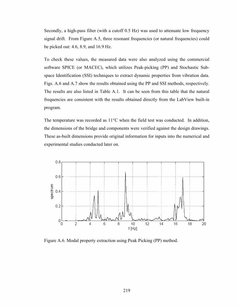
219
Secondly, a high-pass filter (with a cutoff 0.5 Hz) was used to attenuate low frequency
signal drift. From Figure A.5, three resonant frequencies (or natural frequencies) could
be picked out: 4.6, 8.9, and 16.9 Hz.
To check these values, the measured data were also analyzed using the commercial
software SPICE (or MACEC), which utilizes Peak-picking (PP) and Stochastic Sub-
space Identification (SSI) techniques to extract dynamic properties from vibration data.
Figs. A.6 and A.7 show the results obtained using the PP and SSI methods, respectively.
The results are also listed in Table A.1. It can be seen from this table that the natural
frequencies are consistent with the results obtained directly from the LabView built-in
program.
The temperature was recorded as 11°C when the field test was conducted. In addition,
the dimensions of the bridge and components were verified against the design drawings.
These as-built dimensions provide original information for inputs into the numerical and
experimental studies conducted later on.
Figure A.6. Modal property extraction using Peak Picking (PP) method.

220
Table A.1. The measured natural frequencies of the prototype bridge using ambient excitation.
Measured natural frequency (Hz) Modal Extraction Methods Mode 1 Mode 2 Mode 3 LabView built-in program 4.6 8.9 16.9 Peak Picking 4.66 8.96 16.99 SSI 4.68 9.03 16.93
Figure A.7. Modal property extraction using Stochastic Subspace Identification (SSI)method.
221
APPENDIX B. PRELIMINARY NUMERICAL STUDIES
B.1 Introduction
The structure used for this investigation was a one-third scale model of a slab-on-girder
composite bridge superstructure featuring four steel girders supporting a steel-free
concrete deck. The model was based on a prototype superstructure forming part of the
North Perimeter Red River Bridge located in Winnipeg, Manitoba.
Prior to constructing the laboratory model, a preliminary numerical study was carried
out to investigate the appropriate scaling model method to ensure that the dynamic
behaviour of the laboratory mode could reproduce that of the prototype. Therefore, it
was necessary to investigate a scaling model method to properly scale the laboratory
model from the prototype. Specifically, in this preliminary study, half scale and quarter
scale models were initially selected to verify the scaling model method, even though a
one-third scale model was built finally based on the available space in the structural
laboratory of the University of Saskatchewan.
B.2 Scaling Model with Gravitational Force Neglected
The dimensional homogeneity among the physical parameters of the length L, modulus
of elasticity E, gravitational acceleration g, and mass density cannot be satisfied
simultaneously when the bridge deck is scaled, because there are only three independent
basic quantities (fundamental dimensions) which can be chosen arbitrarily. In the
VBDD method, the primary variables are natural frequencies and mode shapes.
Gravitational force has little influence on the values of natural frequencies and mode
shapes, suggesting that the influence of the gravitational force can be neglected in the
scaling process. The length L, modulus of elasticity E, and mass density can then be

222
chosen as the independent basic quantities. In that case, there are the following
equations:
mlp LSL
mEp ESE
mp S
where subscripts p and m refer to prototype and model, respectively, and S denotes the
relevant scaling factor. For example, ES denotes the scaling factor for the modulus of
elasticity, relating the prototype and model values. The scaling factors for all other
quantities associated with the model can be calculated from ES , lS and S . Some
scaling relationships for important physical parameters are listed in Table B.1.
Table B.1. Similitude requirements for the scale bridge model.
Scaling Parameters Dimension Scaling Factors
Length L Displacement L Force F Time T Frequency T Velocity LT 1
Gravitational acceleration LT Neglected
Acceleration LT Mass density FL T 1
Strain -- 1
Stress FL 1
Modulus of Elasticity FL 1
Poisson’s ratio -- 1
lS
lS2lS
lS1 1
lS1
2
2 1lS
4 2
2
2
223
Modeling with gravitational force neglected is convenient because the same density and
strength values for concrete and structural steel could be used for the scaling model as
that of the prototype bridge. However, a full investigation was needed to determine
whether or not the gravitational force will seriously influence the values of natural
frequencies and mode shapes after the damage is introduced into the bridge deck.
B.3 Finite Element Verification for the Feasibility of the Scaling Model Method
Three sets of scaled 4-girder steel-free bridge deck models were generated using
ANSYS, a commercial finite element (FE) software, including a full scale model, a half
scale model, and a quarter scale model. Undamaged cases, single damage cases, and
multiple damage cases were studied to verify the feasibility of the scaling model method
with gravitational force neglected.
According to the theory of scaling with gravitational force neglected, the length L,
modulus of elasticity E, and mass density were chosen as the independent basic
quantities as discussed previously. For convenience, therefore, scaling factors of 1ES
, and 1ρS were selected. That is, the same elastic modulus and density were used for
the model and prototype. The only parameter which varied between models and
prototype was length, L, which was scaled according to the relationship mlp LSL . In
this study, 1lS , 2lS , and 4lS were selected for the full scale, half scale, and
quarter scale models, respectively.
For the undamaged cases, the values of the frequencies of the full scale, half scale, and
quarter scale models are listed in Table B.2. For single damage cases, the values of the
frequencies of the full scale, half scale, and quarter scale models are listed in Table B.3.
These results demonstrate that the natural frequencies scaled as expected in all cases
(i.e. properly scaled natural frequencies of the scale models matched full scale values).
Therefore, it was concluded that scaling by ignoring gravitational forces was valid for
dynamic testing.

224
B.4 Conclusions
For scaling model properties from prototype values, it was found that using the
approach in which gravitational forces were neglected produced the similitude relation
for natural frequency of 1 lf SS which was found to be satisfied very well before and
after damage introduced. Therefore, the scaling model with gravitational force
neglected was demonstrated to be an appropriate scaling method for the VBDD study.
Table B.3. The natural frequencies (Hz) for a single-damage case on the 4-girder steel free bridge deck.
Mode No. Full Scale
(Frequency f)
Half Scale ( 2lS ) Quarter Scale ( 4lS )
f 1 lSf f 1 lSf
1 3.3745 6.7491 3.37455 13.497 3.37425 2 4.8814 9.7628 4.8814 19.525 4.88125 3 9.2705 18.541 9.2705 37.090 9.2725 4 12.714 25.428 12.714 50.852 12.713 5 14.861 29.723 14.8615 59.443 14.86075
Table B.2. The natural frequencies (Hz) of the undamaged 4-girder steel free bridge deck.
Mode No. Full Scale
(Frequency f)
Half Scale ( 2lS ) Quarter Scale ( 4lS )
f 1 lSf f 1 lSf
1 3.3772 6.7545 3.37725 13.507 3.37675 2 4.8881 9.7762 4.8881 19.551 4.88775 3 9.3131 18.626 9.313 37.260 9.315 4 12.733 25.465 12.7325 50.926 12.7315 5 14.878 29.757 14.8785 59.511 14.87775

225
APPENDIX C. FABRICATION OF EXPERIMENTAL
MODEL
In this appendix, some information related to the fabrication of the experimental model,
including the measured compressive strength of concrete samples used for the bridge
deck, the fabrication of the steel superstructure of the bridge model, and the construction
process of the concrete deck, is presented.
Table C.1. The measured compressive strength of concrete samples used for the bridge deck.
Sample No. Beaking force (kN) Compressive strength (MPa) A1 266.88 34.00 A2 306.91 39.10 A3 244.64 31.16 B1 271.33 34.56 B2 275.78 35.13 B3 235.74 30.03 C1 266.88 34.00 C2 269.10 34.28 C3 240.19 30.60
Avg. 264.16 33.65 STDEV 21.84 2.78 C.O.V. 8.27% 8.27%
Avg. = Average; STDEV = Standard deviation; C.O.V. = Coefficient of variation. Notes:
a. The design strength of concrete is 30 MPa; b. Nine concrete cylinders, with a diameter of 100 mm and a height of 200 mm,
were cast on December 20, 2006; c. The samples were moist-cured for 28 days; d. The cylinders were tested on January 17, 2007.

226
Figure C.1. Fabrication of steel superstructure of the bridge model: (a) bolt connectedgirder splice, (b) cross bracing diaphragm, (c) shear studs, (d) bolt connected steel strapsplice, (e) extra channel member with shear studs at the end of the girders, and (f) thefabricated whole steel superstructure.
(a) (b)
(c) (d)
(e) (f)

227
Figure C.2. Construction of the concrete deck of the bridge model: (a) formwork, (b)FRP rebars, (c) pouring concrete, (d) curing concrete, (e) testing a concrete cylinder, and(f) the finished composite bridge model.
(a) (b)
(c) (d)
(e) (f)
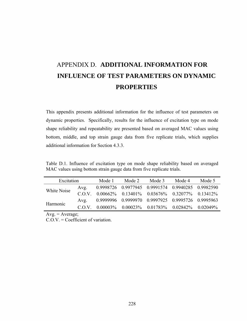
228
APPENDIX D. ADDITIONAL INFORMATION FOR
INFLUENCE OF TEST PARAMETERS ON DYNAMIC
PROPERTIES
This appendix presents additional information for the influence of test parameters on
dynamic properties. Specifically, results for the influence of excitation type on mode
shape reliability and repeatability are presented based on averaged MAC values using
bottom, middle, and top strain gauge data from five replicate trials, which supplies
additional information for Section 4.3.3.
Table D.1. Influence of excitation type on mode shape reliability based on averaged MAC values using bottom strain gauge data from five replicate trials.
Excitation Mode 1 Mode 2 Mode 3 Mode 4 Mode 5
White Noise Avg. 0.9998726 0.9977945 0.9991574 0.9940285 0.9982590C.O.V. 0.00662% 0.13401% 0.03676% 0.32077% 0.13412%
Harmonic Avg. 0.9999996 0.9999970 0.9997925 0.9995726 0.9995963
C.O.V. 0.00003% 0.00023% 0.01783% 0.02842% 0.02049%
Avg. = Average; C.O.V. = Coefficient of variation.

229
Table D.3. Influence of excitation type on mode shape reliability based on averaged MAC values using top strain gauge data from five replicate trials.
Excitation Mode 1 Mode 2 Mode 3 Mode 4 Mode 5
White Noise Avg. 0.9992558 0.9850748 0.9987266 0.9899599 0.9956863C.O.V. 0.04638% 1.11304% 0.07789% 0.65779% 0.18205%
Harmonic Avg. 0.9999984 0.9999757 0.9984081 0.9333263 0.9900844
C.O.V. 0.00010% 0.00087% 0.06939% 3.19241% 0.70144%
Avg. = Average; C.O.V. = Coefficient of variation.
Table D.2. Influence of excitation type on mode shape reliability based on averaged MAC values using middle strain gauge data from five replicate trials.
Excitation Mode 1 Mode 2 Mode 3 Mode 4 Mode 5
White Noise Avg. 0.9994881 0.9939806 0.9991072 0.9936696 0.9977089C.O.V. 0.04697% 0.50404% 0.04621% 0.34150% 0.15767%
Harmonic Avg. 0.9999989 0.9999921 0.9998106 0.9970549 0.9990439
C.O.V. 0.00004% 0.00038% 0.01404% 0.19892% 0.08378%
Avg. = Average; C.O.V. = Coefficient of variation.

230
APPENDIX E. EVALUATION OF EXTRACTED
DYNAMIC PROPERTIES
This appendix presents additional information for Chapter 4. Specifically, Tables E.1 to
E.16 present the lowest five natural frequencies of the bridge model in Health States 2 to
17, extracted from the accelerometer data in five trials, as obtained using the white noise
random excitation, which supplies additional information for Table 4.1.
Tables E.17 to E.32 present the lowest five natural frequencies of the bridge model in
Health States 2 to 17, extracted from the strain gauge data in five trials, as obtained
using the white noise random excitation, which supplies additional information for
Table 4.2.
Figure E.1 presents exactly the same mode shapes as presented in Fig. 4.10. However, a
different figure style was used for this figure to understand the mode shapes better.
Figures E.2 to E.13 present additional information for Section 4.2.4, including
comparisons of the measured mode shapes in different health states using white noise
random excitation, strain gauge data, and higher modes.

231
Table E.1. Measured natural frequencies using accelerometers for Health State 2.
Trials Setups
Measured natural frequency (Hz)
Mode 1 Mode 2 Mode 3 Mode 4 Mode 5
Trial 1
Set 1_1 12.628 13.718 34.450 35.677 38.701 Set 2_1 12.650 13.720 34.505 35.734 38.600 Set 3_1 12.634 13.699 34.470 35.616 38.598 Set 4_1 12.622 13.713 34.499 35.663 38.652 Set 5_1 12.630 13.708 34.603 35.793 38.681
Average (Hz) 12.633 13.712 34.506 35.697 38.646
Trial 2
Set 1_2 12.631 13.720 34.465 35.650 38.614 Set 2_2 12.628 13.712 34.543 35.616 38.672 Set 3_2 12.624 13.707 34.450 35.602 38.575 Set 4_2 12.623 13.709 34.491 35.621 38.727 Set 5_2 12.620 13.715 34.624 35.759 38.728
Average (Hz) 12.625 13.713 34.515 35.650 38.663
Trial 3
Set 1_3 12.629 13.720 34.522 35.750 38.656 Set 2_3 12.623 13.719 34.537 35.693 38.638 Set 3_3 12.633 13.696 34.482 35.610 38.577 Set 4_3 12.626 13.708 34.500 35.653 38.662 Set 5_3 12.625 13.709 34.581 35.769 38.663
Average (Hz) 12.627 13.710 34.524 35.695 38.639
Trial 4
Set 1_4 12.608 13.704 34.501 35.664 38.592 Set 2_4 12.629 13.710 34.506 35.705 38.620 Set 3_4 12.615 13.692 34.472 35.674 38.644 Set 4_4 12.616 13.692 34.518 35.653 38.615 Set 5_4 12.634 13.718 34.601 35.744 38.675
Average (Hz) 12.620 13.703 34.520 35.688 38.629
Trial 5
Set 1_5 12.629 13.710 34.504 35.708 38.700 Set 2_5 12.621 13.700 34.498 35.720 38.677 Set 3_5 12.626 13.694 34.507 35.690 38.654 Set 4_5 12.630 13.707 34.501 35.661 38.683 Set 5_5 12.623 13.712 34.594 35.700 38.603
Average (Hz) 12.626 13.704 34.521 35.696 38.664
All Data Average (Hz) 12.626 13.708 34.517 35.685 38.648 STDEV (Hz) 0.008 0.009 0.049 0.053 0.044
C.O.V. 0.06% 0.06% 0.14% 0.15% 0.11% STDEV = Standard deviation; C.O.V. = Coefficient of variation.

232
Table E.2. Measured natural frequencies using accelerometers for Health State 3.
Trials Setups
Measured natural frequency (Hz)
Mode 1 Mode 2 Mode 3 Mode 4 Mode 5
Trial 1
Set 1_1 12.602 13.700 30.027 34.176 38.681 Set 2_1 12.628 13.712 30.100 34.159 38.622 Set 3_1 12.605 13.687 30.082 34.102 38.569 Set 4_1 12.631 13.744 30.097 34.210 38.753 Set 5_1 12.612 13.677 30.067 34.080 38.581
Average (Hz) 12.615 13.704 30.075 34.146 38.641
Trial 2
Set 1_2 12.590 13.709 30.094 34.109 38.676 Set 2_2 12.607 13.696 30.096 34.143 38.690 Set 3_2 12.623 13.694 30.088 34.098 38.324 Set 4_2 12.624 13.730 30.152 34.222 38.711 Set 5_2 12.612 13.676 30.082 34.094 38.624
Average (Hz) 12.611 13.701 30.102 34.133 38.605
Trial 3
Set 1_3 12.624 13.705 30.064 34.168 38.732 Set 2_3 12.607 13.688 30.047 34.116 38.788 Set 3_3 12.608 13.690 30.066 34.125 38.606 Set 4_3 12.597 13.740 30.159 34.249 38.692 Set 5_3 12.595 13.683 30.055 34.133 38.553
Average (Hz) 12.606 13.701 30.078 34.158 38.674
Trial 4
Set 1_4 12.606 13.728 30.089 34.138 38.748 Set 2_4 12.603 13.697 30.085 34.156 38.631 Set 3_4 12.596 13.707 30.064 34.131 38.504 Set 4_4 12.625 13.737 30.135 34.199 38.636 Set 5_4 12.607 13.682 30.053 34.169 38.555
Average (Hz) 12.607 13.711 30.085 34.159 38.615
Trial 5
Set 1_5 12.615 13.702 30.104 34.165 38.514 Set 2_5 12.607 13.694 30.085 34.122 38.676 Set 3_5 12.600 13.695 30.042 34.137 38.512 Set 4_5 12.617 13.729 30.133 34.250 38.573 Set 5_5 12.601 13.680 30.036 34.141 38.592
Average (Hz) 12.608 13.700 30.080 34.163 38.573
All Data Average (Hz) 12.610 13.703 30.084 34.152 38.622 STDEV (Hz) 0.011 0.021 0.034 0.046 0.101
C.O.V. 0.09% 0.15% 0.11% 0.13% 0.26% STDEV = Standard deviation; C.O.V. = Coefficient of variation.

233
Table E.3. Measured natural frequencies using accelerometers for Health State 4.
Trials Setups
Measured natural frequency (Hz)
Mode 1 Mode 2 Mode 3 Mode 4 Mode 5
Trial 1
Set 1_1 12.604 13.699 29.977 33.863 34.717 Set 2_1 12.613 13.705 29.996 33.891 35.093 Set 3_1 12.587 13.686 30.025 33.853 34.951 Set 4_1 12.603 13.697 29.907 33.881 34.764 Set 5_1 12.616 13.697 30.013 33.889 34.808
Average (Hz) 12.605 13.697 29.983 33.875 34.867
Trial 2
Set 1_2 12.619 13.695 29.958 33.889 34.644 Set 2_2 12.612 13.682 30.019 33.888 35.139 Set 3_2 12.602 13.697 30.022 33.886 34.838 Set 4_2 12.585 13.711 29.994 33.863 34.766 Set 5_2 12.600 13.700 29.900 33.900 34.700
Average (Hz) 12.603 13.697 29.979 33.885 34.817
Trial 3
Set 1_3 12.605 13.711 29.911 33.838 34.899 Set 2_3 12.597 13.709 30.000 33.918 35.386 Set 3_3 12.604 13.695 29.997 33.867 34.861 Set 4_3 12.621 13.685 29.986 33.889 34.722 Set 5_3 12.600 13.700 30.100 33.800 34.800
Average (Hz) 12.605 13.700 29.999 33.863 34.934
Trial 4
Set 1_4 12.598 13.720 30.059 33.858 34.751 Set 2_4 12.613 13.686 30.007 33.789 35.149 Set 3_4 12.596 13.724 29.995 33.862 34.801 Set 4_4 12.610 13.683 30.015 33.798 34.757 Set 5_4 12.600 13.700 30.000 33.900 34.800
Average (Hz) 12.604 13.703 30.015 33.842 34.852
Trial 5
Set 1_5 12.606 13.688 30.013 33.954 34.997 Set 2_5 12.608 13.710 29.971 33.845 35.413 Set 3_5 12.594 13.699 30.023 33.829 34.933 Set 4_5 12.623 13.692 30.029 33.888 34.753 Set 5_5 12.600 13.700 30.000 33.800 34.800
Average (Hz) 12.606 13.698 30.007 33.863 34.979
All Data Average (Hz) 12.605 13.699 29.997 33.866 34.890 STDEV (Hz) 0.010 0.011 0.044 0.040 0.203
C.O.V. 0.08% 0.08% 0.15% 0.12% 0.58% STDEV = Standard deviation; C.O.V. = Coefficient of variation.

234
Table E.4. Measured natural frequencies using accelerometers for Health State 5.
Trials Setups
Measured natural frequency (Hz)
Mode 1 Mode 2 Mode 3 Mode 4 Mode 5
Trial 1
Set 1_1 12.584 13.713 29.953 34.267 38.611 Set 2_1 12.595 13.745 29.945 34.357 38.639 Set 3_1 12.598 13.754 29.931 34.227 38.498 Set 4_1 12.624 13.815 30.014 34.436 38.877 Set 5_1 12.604 13.715 29.885 34.224 38.250
Average (Hz) 12.601 13.749 29.946 34.302 38.575
Trial 2
Set 1_2 12.594 13.742 29.947 34.162 38.504 Set 2_2 12.607 13.731 29.950 34.321 38.759 Set 3_2 12.577 13.752 29.926 34.228 38.464 Set 4_2 12.628 13.802 29.987 34.430 38.934 Set 5_2 12.581 13.718 29.939 34.222 38.386
Average (Hz) 12.597 13.749 29.950 34.272 38.609
Trial 3
Set 1_3 12.576 13.747 29.975 34.174 38.597 Set 2_3 12.591 13.745 29.940 34.294 38.656 Set 3_3 12.586 13.750 30.009 34.338 38.464 Set 4_3 12.629 13.798 30.087 34.109 38.944 Set 5_3 12.582 13.730 29.931 34.145 38.498
Average (Hz) 12.593 13.754 29.988 34.212 38.632
Trial 4
Set 1_4 12.593 13.735 29.944 34.204 38.455 Set 2_4 12.605 13.748 29.964 34.244 38.660 Set 3_4 12.588 13.752 29.984 34.410 38.620 Set 4_4 12.636 13.798 29.954 34.359 38.735 Set 5_4 12.597 13.734 29.911 34.195 38.592
Average (Hz) 12.604 13.753 29.951 34.282 38.612
Trial 5
Set 1_5 12.610 13.747 29.926 34.167 38.534 Set 2_5 12.596 13.748 29.936 34.288 38.558 Set 3_5 12.585 13.745 29.950 34.417 38.488 Set 4_5 12.633 13.799 29.933 34.454 38.814 Set 5_5 12.573 13.736 29.945 34.217 38.586
Average (Hz) 12.599 13.755 29.938 34.309 38.596
All Data Average (Hz) 12.599 13.752 29.955 34.276 38.605 STDEV (Hz) 0.019 0.028 0.040 0.101 0.168
C.O.V. 0.15% 0.21% 0.13% 0.29% 0.44% STDEV = Standard deviation; C.O.V. = Coefficient of variation.

235
Table E.5. Measured natural frequencies using accelerometers for Health State 6.
Trials Setups
Measured natural frequency (Hz)
Mode 1 Mode 2 Mode 3 Mode 4 Mode 5
Trial 1
Set 1_1 12.568 13.733 34.022 35.677 38.824 Set 2_1 12.617 13.762 34.025 35.814 38.928 Set 3_1 12.590 13.725 34.042 35.711 38.891 Set 4_1 12.608 13.746 34.043 35.715 38.844 Set 5_1 12.608 13.789 34.239 35.926 39.074
Average (Hz) 12.598 13.751 34.074 35.768 38.912
Trial 2
Set 1_2 12.582 13.761 34.090 35.889 38.832 Set 2_2 12.609 13.749 33.984 35.755 38.941 Set 3_2 12.595 13.746 33.976 35.667 38.840 Set 4_2 12.582 13.745 34.097 35.807 38.970 Set 5_2 12.604 13.799 34.175 35.922 39.103
Average (Hz) 12.594 13.760 34.064 35.808 38.937
Trial 3
Set 1_3 12.594 13.752 33.959 35.809 38.885 Set 2_3 12.605 13.750 33.994 35.822 38.869 Set 3_3 12.600 13.743 33.986 35.782 38.770 Set 4_3 12.611 13.748 34.190 35.751 38.891 Set 5_3 12.596 13.779 34.282 35.983 39.030
Average (Hz) 12.601 13.754 34.082 35.829 38.889
Trial 4
Set 1_4 12.580 13.715 34.078 35.798 38.821 Set 2_4 12.592 13.741 33.974 35.809 38.869 Set 3_4 12.603 13.729 34.074 35.743 38.764 Set 4_4 12.607 13.745 34.119 35.696 38.967 Set 5_4 12.585 13.806 34.277 35.910 39.145
Average (Hz) 12.593 13.747 34.104 35.791 38.913
Trial 5
Set 1_5 12.590 13.754 34.016 35.835 38.785 Set 2_5 12.590 13.768 33.987 35.787 38.783 Set 3_5 12.588 13.736 34.057 35.750 38.816 Set 4_5 12.591 13.739 34.106 35.682 38.925 Set 5_5 12.602 13.794 34.174 35.781 38.966
Average (Hz) 12.592 13.758 34.068 35.767 38.855
All Data Average (Hz) 12.596 13.754 34.079 35.793 38.901 STDEV (Hz) 0.012 0.023 0.096 0.084 0.104
C.O.V. 0.09% 0.17% 0.28% 0.23% 0.27% STDEV = Standard deviation; C.O.V. = Coefficient of variation.

236
Table E.6. Measured natural frequencies using accelerometers for Health State 7.
Trials Setups
Measured natural frequency (Hz)
Mode 1 Mode 2 Mode 3 Mode 4 Mode 5
Trial 1
Set 1_1 12.555 13.718 33.572 35.749 38.863 Set 2_1 12.584 13.719 33.696 35.953 38.814 Set 3_1 12.580 13.729 33.767 35.870 38.812 Set 4_1 12.598 13.739 33.925 35.951 39.011 Set 5_1 12.605 13.746 33.662 35.777 38.885
Average (Hz) 12.584 13.730 33.724 35.860 38.877
Trial 2
Set 1_2 12.592 13.728 33.653 35.742 38.816 Set 2_2 12.585 13.737 33.773 35.951 38.943 Set 3_2 12.569 13.715 33.803 35.869 38.904 Set 4_2 12.593 13.746 33.994 35.880 39.059 Set 5_2 12.576 13.747 33.619 35.670 38.842
Average (Hz) 12.583 13.735 33.768 35.822 38.913
Trial 3
Set 1_3 12.600 13.723 33.633 35.709 38.888 Set 2_3 12.573 13.730 33.803 35.861 38.830 Set 3_3 12.553 13.726 33.803 35.896 38.920 Set 4_3 12.587 13.762 33.942 35.940 39.020 Set 5_3 12.587 13.744 33.664 35.802 38.983
Average (Hz) 12.580 13.737 33.769 35.841 38.928
Trial 4
Set 1_4 12.575 13.709 33.600 35.696 38.864 Set 2_4 12.584 13.740 33.757 35.860 38.848 Set 3_4 12.583 13.722 33.768 35.893 38.882 Set 4_4 12.582 13.742 33.957 35.933 39.105 Set 5_4 12.584 13.735 33.645 35.733 38.899
Average (Hz) 12.582 13.729 33.745 35.823 38.919
Trial 5
Set 1_5 12.590 13.718 33.615 35.697 38.899 Set 2_5 12.574 13.733 33.808 35.960 38.969 Set 3_5 12.588 13.723 33.734 35.892 38.905 Set 4_5 12.591 13.748 33.988 35.917 39.030 Set 5_5 12.586 13.732 33.694 35.866 38.990
Average (Hz) 12.586 13.731 33.768 35.866 38.958
All Data Average (Hz) 12.583 13.732 33.755 35.843 38.919 STDEV (Hz) 0.012 0.013 0.127 0.094 0.082
C.O.V. 0.10% 0.09% 0.37% 0.26% 0.21% STDEV = Standard deviation; C.O.V. = Coefficient of variation.

237
Table E.7. Measured natural frequencies using accelerometers for Health State 8.
Trials Setups
Measured natural frequency (Hz)
Mode 1 Mode 2 Mode 3 Mode 4 Mode 5
Trial 1
Set 1_1 12.565 13.738 31.071 34.496 38.916 Set 2_1 12.602 13.764 31.036 34.492 38.715 Set 3_1 12.573 13.752 31.117 34.666 38.762 Set 4_1 12.588 13.749 31.061 34.810 38.900 Set 5_1 12.608 13.761 31.095 34.694 38.899
Average (Hz) 12.587 13.752 31.076 34.632 38.838
Trial 2
Set 1_2 12.582 13.765 31.068 34.611 38.889 Set 2_2 12.591 13.755 31.010 34.698 38.765 Set 3_2 12.574 13.730 31.053 34.672 38.797 Set 4_2 12.591 13.758 31.064 34.868 38.990 Set 5_2 12.581 13.735 31.107 34.760 38.919
Average (Hz) 12.584 13.749 31.061 34.722 38.872
Trial 3
Set 1_3 12.574 13.718 31.108 34.666 38.817 Set 2_3 12.594 13.752 31.052 34.573 38.694 Set 3_3 12.597 13.762 30.992 34.759 38.729 Set 4_3 12.590 13.774 31.142 34.821 39.130 Set 5_3 12.593 13.767 31.051 34.656 38.881
Average (Hz) 12.590 13.754 31.069 34.695 38.850
Trial 4
Set 1_4 12.566 13.756 31.056 34.710 38.890 Set 2_4 12.585 13.751 31.093 34.695 38.707 Set 3_4 12.573 13.756 31.070 34.735 38.679 Set 4_4 12.567 13.773 31.014 34.837 38.992 Set 5_4 12.612 13.756 31.113 34.631 38.928
Average (Hz) 12.581 13.758 31.069 34.722 38.839
Trial 5
Set 1_5 12.585 13.737 31.095 34.606 38.855 Set 2_5 12.558 13.734 31.062 34.615 38.603 Set 3_5 12.571 13.753 31.059 34.655 38.692 Set 4_5 12.573 13.774 31.081 34.827 39.067 Set 5_5 12.581 13.746 31.090 34.708 38.951
Average (Hz) 12.574 13.749 31.077 34.682 38.834
All Data Average (Hz) 12.583 13.753 31.070 34.690 38.847 STDEV (Hz) 0.014 0.014 0.035 0.098 0.131
C.O.V. 0.11% 0.10% 0.11% 0.28% 0.34% STDEV = Standard deviation; C.O.V. = Coefficient of variation.

238
Table E.8. Measured natural frequencies using accelerometers for Health State 9.
Trials Setups
Measured natural frequency (Hz)
Mode 1 Mode 2 Mode 3 Mode 4 Mode 5
Trial 1
Set 1_1 12.580 13.703 34.511 35.805 39.006 Set 2_1 12.592 13.721 34.568 35.981 39.126 Set 3_1 12.569 13.723 34.620 35.903 39.028 Set 4_1 12.625 13.763 34.730 35.812 39.183 Set 5_1 12.585 13.737 34.602 35.845 39.044
Average (Hz) 12.590 13.729 34.606 35.869 39.077
Trial 2
Set 1_2 12.603 13.700 34.567 35.807 39.056 Set 2_2 12.604 13.736 34.563 35.795 39.010 Set 3_2 12.581 13.731 34.539 35.799 39.008 Set 4_2 12.621 13.754 34.632 35.857 39.218 Set 5_2 12.582 13.719 34.603 35.772 39.133
Average (Hz) 12.598 13.728 34.581 35.806 39.085
Trial 3
Set 1_3 12.577 13.702 34.541 35.756 39.057 Set 2_3 12.591 13.727 34.532 35.867 38.990 Set 3_3 12.609 13.732 34.527 35.824 38.917 Set 4_3 12.608 13.770 34.664 35.807 39.279 Set 5_3 12.616 13.725 34.617 35.686 39.040
Average (Hz) 12.600 13.731 34.576 35.788 39.057
Trial 4
Set 1_4 12.594 13.716 34.527 35.741 39.070 Set 2_4 12.582 13.747 34.536 35.896 39.077 Set 3_4 12.589 13.727 34.542 35.775 38.906 Set 4_4 12.612 13.735 34.625 35.742 39.281 Set 5_4 12.597 13.722 34.703 35.785 38.942
Average (Hz) 12.595 13.730 34.586 35.788 39.055
Trial 5
Set 1_5 12.579 13.711 34.478 35.829 38.984 Set 2_5 12.603 13.757 34.510 35.905 39.101 Set 3_5 12.567 13.735 34.494 35.830 39.022 Set 4_5 12.626 13.763 34.639 35.770 39.175 Set 5_5 12.589 13.747 34.544 35.756 39.077
Average (Hz) 12.593 13.743 34.533 35.818 39.072
All Data Average (Hz) 12.595 13.732 34.577 35.814 39.069 STDEV (Hz) 0.017 0.019 0.065 0.064 0.100
C.O.V. 0.13% 0.14% 0.19% 0.18% 0.26% STDEV = Standard deviation; C.O.V. = Coefficient of variation.

239
Table E.9. Measured natural frequencies using accelerometers for Health State 10.
Trials Setups
Measured natural frequency (Hz)
Mode 1 Mode 2 Mode 3 Mode 4 Mode 5
Trial 1
Set 1_1 12.594 13.715 34.538 35.792 39.074 Set 2_1 12.584 13.710 34.531 35.892 39.071 Set 3_1 12.583 13.735 34.528 35.834 39.097 Set 4_1 12.583 13.704 34.487 35.690 39.019 Set 5_1 12.593 13.720 34.539 35.767 39.019
Average (Hz) 12.587 13.717 34.525 35.795 39.056
Trial 2
Set 1_2 12.599 13.728 34.478 35.768 39.099 Set 2_2 12.579 13.712 34.483 35.804 39.051 Set 3_2 12.581 13.728 34.537 35.842 39.061 Set 4_2 12.595 13.733 34.554 35.804 39.101 Set 5_2 12.605 13.722 34.560 35.821 39.089
Average (Hz) 12.592 13.725 34.523 35.808 39.080
Trial 3
Set 1_3 12.597 13.714 34.504 35.794 38.964 Set 2_3 12.596 13.700 34.568 35.910 39.011 Set 3_3 12.594 13.742 34.583 35.974 39.088 Set 4_3 12.592 13.734 34.446 35.740 39.076 Set 5_3 12.587 13.726 34.562 35.804 38.993
Average (Hz) 12.593 13.723 34.532 35.844 39.027
Trial 4
Set 1_4 12.590 13.735 34.513 35.780 39.144 Set 2_4 12.609 13.725 34.487 35.881 39.086 Set 3_4 12.590 13.732 34.530 35.806 39.016 Set 4_4 12.575 13.734 34.462 35.811 39.046 Set 5_4 12.599 13.734 34.483 35.768 38.962
Average (Hz) 12.593 13.732 34.495 35.809 39.051
Trial 5
Set 1_5 12.593 13.700 34.559 35.770 39.051 Set 2_5 12.581 13.725 34.471 35.824 38.908 Set 3_5 12.583 13.729 34.471 35.780 38.967 Set 4_5 12.595 13.725 34.554 35.754 39.037 Set 5_5 12.587 13.736 34.532 35.686 39.016
Average (Hz) 12.588 13.723 34.517 35.763 38.996
All Data Average (Hz) 12.591 13.724 34.518 35.804 39.042 STDEV (Hz) 0.008 0.012 0.038 0.064 0.055
C.O.V. 0.07% 0.09% 0.11% 0.18% 0.14% STDEV = Standard deviation; C.O.V. = Coefficient of variation.
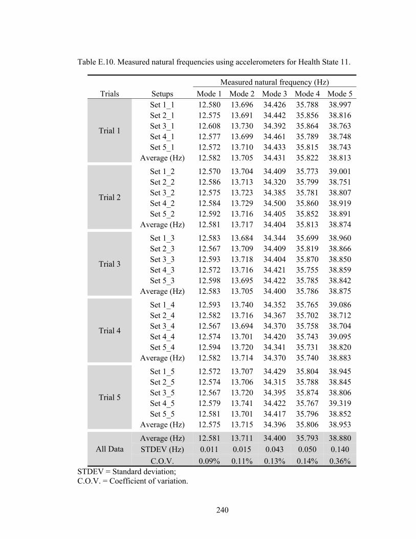
240
Table E.10. Measured natural frequencies using accelerometers for Health State 11.
Trials Setups
Measured natural frequency (Hz)
Mode 1 Mode 2 Mode 3 Mode 4 Mode 5
Trial 1
Set 1_1 12.580 13.696 34.426 35.788 38.997 Set 2_1 12.575 13.691 34.442 35.856 38.816 Set 3_1 12.608 13.730 34.392 35.864 38.763 Set 4_1 12.577 13.699 34.461 35.789 38.748 Set 5_1 12.572 13.710 34.433 35.815 38.743
Average (Hz) 12.582 13.705 34.431 35.822 38.813
Trial 2
Set 1_2 12.570 13.704 34.409 35.773 39.001 Set 2_2 12.586 13.713 34.320 35.799 38.751 Set 3_2 12.575 13.723 34.385 35.781 38.807 Set 4_2 12.584 13.729 34.500 35.860 38.919 Set 5_2 12.592 13.716 34.405 35.852 38.891
Average (Hz) 12.581 13.717 34.404 35.813 38.874
Trial 3
Set 1_3 12.583 13.684 34.344 35.699 38.960 Set 2_3 12.567 13.709 34.409 35.819 38.866 Set 3_3 12.593 13.718 34.404 35.870 38.850 Set 4_3 12.572 13.716 34.421 35.755 38.859 Set 5_3 12.598 13.695 34.422 35.785 38.842
Average (Hz) 12.583 13.705 34.400 35.786 38.875
Trial 4
Set 1_4 12.593 13.740 34.352 35.765 39.086 Set 2_4 12.582 13.716 34.367 35.702 38.712 Set 3_4 12.567 13.694 34.370 35.758 38.704 Set 4_4 12.574 13.701 34.420 35.743 39.095 Set 5_4 12.594 13.720 34.341 35.731 38.820
Average (Hz) 12.582 13.714 34.370 35.740 38.883
Trial 5
Set 1_5 12.572 13.707 34.429 35.804 38.945 Set 2_5 12.574 13.706 34.315 35.788 38.845 Set 3_5 12.567 13.720 34.395 35.874 38.806 Set 4_5 12.579 13.741 34.422 35.767 39.319 Set 5_5 12.581 13.701 34.417 35.796 38.852
Average (Hz) 12.575 13.715 34.396 35.806 38.953
All Data Average (Hz) 12.581 13.711 34.400 35.793 38.880 STDEV (Hz) 0.011 0.015 0.043 0.050 0.140
C.O.V. 0.09% 0.11% 0.13% 0.14% 0.36% STDEV = Standard deviation; C.O.V. = Coefficient of variation.
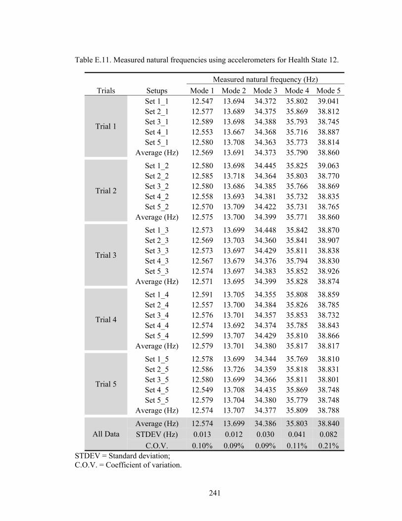
241
Table E.11. Measured natural frequencies using accelerometers for Health State 12.
Trials Setups
Measured natural frequency (Hz)
Mode 1 Mode 2 Mode 3 Mode 4 Mode 5
Trial 1
Set 1_1 12.547 13.694 34.372 35.802 39.041 Set 2_1 12.577 13.689 34.375 35.869 38.812 Set 3_1 12.589 13.698 34.388 35.793 38.745 Set 4_1 12.553 13.667 34.368 35.716 38.887 Set 5_1 12.580 13.708 34.363 35.773 38.814
Average (Hz) 12.569 13.691 34.373 35.790 38.860
Trial 2
Set 1_2 12.580 13.698 34.445 35.825 39.063 Set 2_2 12.585 13.718 34.364 35.803 38.770 Set 3_2 12.580 13.686 34.385 35.766 38.869 Set 4_2 12.558 13.693 34.381 35.732 38.835 Set 5_2 12.570 13.709 34.422 35.731 38.765
Average (Hz) 12.575 13.700 34.399 35.771 38.860
Trial 3
Set 1_3 12.573 13.699 34.448 35.842 38.870 Set 2_3 12.569 13.703 34.360 35.841 38.907 Set 3_3 12.573 13.697 34.429 35.811 38.838 Set 4_3 12.567 13.679 34.376 35.794 38.830 Set 5_3 12.574 13.697 34.383 35.852 38.926
Average (Hz) 12.571 13.695 34.399 35.828 38.874
Trial 4
Set 1_4 12.591 13.705 34.355 35.808 38.859 Set 2_4 12.557 13.700 34.384 35.826 38.785 Set 3_4 12.576 13.701 34.357 35.853 38.732 Set 4_4 12.574 13.692 34.374 35.785 38.843 Set 5_4 12.599 13.707 34.429 35.810 38.866
Average (Hz) 12.579 13.701 34.380 35.817 38.817
Trial 5
Set 1_5 12.578 13.699 34.344 35.769 38.810 Set 2_5 12.586 13.726 34.359 35.818 38.831 Set 3_5 12.580 13.699 34.366 35.811 38.801 Set 4_5 12.549 13.708 34.435 35.869 38.748 Set 5_5 12.579 13.704 34.380 35.779 38.748
Average (Hz) 12.574 13.707 34.377 35.809 38.788
All Data Average (Hz) 12.574 13.699 34.386 35.803 38.840 STDEV (Hz) 0.013 0.012 0.030 0.041 0.082
C.O.V. 0.10% 0.09% 0.09% 0.11% 0.21% STDEV = Standard deviation; C.O.V. = Coefficient of variation.

242
Table E.12. Measured natural frequencies using accelerometers for Health State 13.
Trials Setups
Measured natural frequency (Hz)
Mode 1 Mode 2 Mode 3 Mode 4 Mode 5
Trial 1
Set 1_1 12.631 13.890 34.252 36.056 38.679 Set 2_1 12.627 13.903 34.193 36.095 38.571 Set 3_1 12.628 13.892 34.334 36.131 38.586 Set 4_1 12.639 13.883 34.359 36.132 38.647 Set 5_1 12.616 13.863 34.273 36.064 38.547
Average (Hz) 12.628 13.886 34.282 36.096 38.606
Trial 2
Set 1_2 12.635 13.880 34.345 36.075 38.677 Set 2_2 12.625 13.880 34.321 36.042 38.563 Set 3_2 12.632 13.900 34.335 36.090 38.669 Set 4_2 12.630 13.882 34.312 36.107 38.625 Set 5_2 12.618 13.887 34.226 36.069 38.509
Average (Hz) 12.628 13.886 34.308 36.076 38.609
Trial 3
Set 1_3 12.620 13.854 34.342 36.025 38.609 Set 2_3 12.633 13.894 34.290 36.081 38.563 Set 3_3 12.628 13.882 34.335 36.111 38.676 Set 4_3 12.634 13.901 34.285 36.079 38.667 Set 5_3 12.637 13.872 34.281 36.087 38.640
Average (Hz) 12.630 13.880 34.307 36.077 38.631
Trial 4
Set 1_4 12.656 13.879 34.315 36.046 38.506 Set 2_4 12.630 13.896 34.285 36.085 38.604 Set 3_4 12.636 13.882 34.339 36.095 38.702 Set 4_4 12.633 13.890 34.331 36.115 38.696 Set 5_4 12.614 13.877 34.313 36.054 38.609
Average (Hz) 12.634 13.885 34.317 36.079 38.623
Trial 5
Set 1_5 12.629 13.876 34.291 36.068 38.514 Set 2_5 12.620 13.886 34.308 36.103 38.620 Set 3_5 12.651 13.888 34.346 36.103 38.678 Set 4_5 12.622 13.896 34.305 36.046 38.855 Set 5_5 12.622 13.885 34.284 36.041 38.600
Average (Hz) 12.629 13.886 34.307 36.072 38.653
All Data Average (Hz) 12.630 13.885 34.304 36.080 38.624 STDEV (Hz) 0.010 0.011 0.039 0.029 0.076
C.O.V. 0.08% 0.08% 0.12% 0.08% 0.20% STDEV = Standard deviation; C.O.V. = Coefficient of variation.

243
Table E.13. Measured natural frequencies using accelerometers for Health State 14.
Trials Setups
Measured natural frequency (Hz)
Mode 1 Mode 2 Mode 3 Mode 4 Mode 5
Trial 1
Set 1_1 12.633 13.896 34.549 36.018 38.897 Set 2_1 12.646 13.907 34.508 36.135 38.934 Set 3_1 12.629 13.917 34.512 36.113 38.837 Set 4_1 12.623 13.893 34.549 36.115 38.941 Set 5_1 12.639 13.901 34.491 36.122 38.892
Average (Hz) 12.634 13.903 34.522 36.101 38.900
Trial 2
Set 1_2 12.641 13.916 34.487 36.084 38.908 Set 2_2 12.629 13.928 34.486 36.141 38.997 Set 3_2 12.639 13.925 34.470 36.133 38.865 Set 4_2 12.632 13.894 34.533 36.095 38.939 Set 5_2 12.619 13.891 34.508 36.128 38.899
Average (Hz) 12.632 13.911 34.497 36.116 38.922
Trial 3
Set 1_3 12.640 13.890 34.529 36.090 38.971 Set 2_3 12.633 13.892 34.536 36.075 38.926 Set 3_3 12.623 13.901 34.507 36.090 38.849 Set 4_3 12.637 13.910 34.496 36.021 38.803 Set 5_3 12.624 13.896 34.447 36.053 38.830
Average (Hz) 12.631 13.898 34.503 36.066 38.876
Trial 4
Set 1_4 12.637 13.873 34.423 36.064 38.889 Set 2_4 12.637 13.914 34.476 36.081 38.832 Set 3_4 12.626 13.916 34.509 36.071 38.733 Set 4_4 12.625 13.914 34.542 36.101 38.919 Set 5_4 12.609 13.904 34.492 36.012 38.819
Average (Hz) 12.627 13.904 34.489 36.066 38.838
Trial 5
Set 1_5 12.652 13.887 34.457 36.127 38.858 Set 2_5 12.641 13.905 34.540 36.054 38.931 Set 3_5 12.627 13.884 34.486 36.146 38.980 Set 4_5 12.633 13.890 34.529 36.062 38.959 Set 5_5 12.635 13.889 34.511 36.109 38.910
Average (Hz) 12.638 13.891 34.505 36.100 38.928
All Data Average (Hz) 12.632 13.901 34.503 36.090 38.893 STDEV (Hz) 0.009 0.014 0.032 0.039 0.062
C.O.V. 0.07% 0.10% 0.09% 0.11% 0.16% STDEV = Standard deviation; C.O.V. = Coefficient of variation.

244
Table E.14. Measured natural frequencies using accelerometers for Health State 15.
Trials Setups
Measured natural frequency (Hz)
Mode 1 Mode 2 Mode 3 Mode 4 Mode 5
Trial 1
Set 1_1 12.632 13.910 34.561 36.059 38.994 Set 2_1 12.624 13.926 34.473 36.072 38.883 Set 3_1 12.636 13.903 34.478 36.060 38.880 Set 4_1 12.633 13.903 34.472 36.044 38.820 Set 5_1 12.613 13.909 34.450 36.104 38.893
Average (Hz) 12.628 13.910 34.487 36.068 38.894
Trial 2
Set 1_2 12.620 13.872 34.480 36.090 39.044 Set 2_2 12.625 13.914 34.479 36.073 38.850 Set 3_2 12.632 13.935 34.528 36.147 38.894 Set 4_2 12.614 13.880 34.498 36.115 39.018 Set 5_2 12.639 13.890 34.519 36.126 38.924
Average (Hz) 12.626 13.898 34.501 36.110 38.946
Trial 3
Set 1_3 12.624 13.946 34.452 36.093 38.959 Set 2_3 12.631 13.893 34.418 36.050 38.907 Set 3_3 12.632 13.935 34.528 36.147 38.894 Set 4_3 12.630 13.871 34.583 36.113 38.931 Set 5_3 12.616 13.897 34.534 36.132 38.922
Average (Hz) 12.627 13.908 34.503 36.107 38.923
Trial 4
Set 1_4 12.635 13.902 34.490 36.101 39.013 Set 2_4 12.635 13.910 34.450 36.080 38.892 Set 3_4 12.605 13.884 34.490 36.107 38.977 Set 4_4 12.628 13.896 34.485 36.080 38.891 Set 5_4 12.617 13.916 34.468 36.084 38.966
Average (Hz) 12.624 13.902 34.477 36.090 38.948
Trial 5
Set 1_5 12.618 13.864 34.472 36.106 38.981 Set 2_5 12.614 13.911 34.487 36.127 38.921 Set 3_5 12.620 13.901 34.437 36.119 38.983 Set 4_5 12.617 13.860 34.521 36.093 38.811 Set 5_5 12.618 13.905 34.451 36.129 38.945
Average (Hz) 12.617 13.888 34.474 36.115 38.928
All Data Average (Hz) 12.624 13.901 34.488 36.098 38.928 STDEV (Hz) 0.009 0.022 0.039 0.029 0.060
C.O.V. 0.07% 0.16% 0.11% 0.08% 0.15% STDEV = Standard deviation; C.O.V. = Coefficient of variation.

245
Table E.15. Measured natural frequencies using accelerometers for Health State 16.
Trials Setups
Measured natural frequency (Hz)
Mode 1 Mode 2 Mode 3 Mode 4 Mode 5
Trial 1
Set 1_1 12.620 13.878 34.543 36.193 38.862 Set 2_1 12.641 13.909 34.557 36.126 38.872 Set 3_1 12.601 13.924 34.377 36.106 38.701 Set 4_1 12.612 13.924 34.526 36.062 38.962 Set 5_1 12.607 13.898 34.357 36.028 38.635
Average (Hz) 12.616 13.907 34.472 36.103 38.806
Trial 2
Set 1_2 12.595 13.883 34.435 36.072 38.719 Set 2_2 12.610 13.928 34.495 36.167 38.912 Set 3_2 12.618 13.895 34.577 36.110 38.777 Set 4_2 12.617 13.918 34.484 36.068 38.885 Set 5_2 12.633 13.918 34.370 36.022 38.727
Average (Hz) 12.615 13.908 34.472 36.088 38.804
Trial 3
Set 1_3 12.608 13.920 34.580 36.096 39.021 Set 2_3 12.625 13.932 34.491 36.284 38.923 Set 3_3 12.610 13.905 34.424 36.121 38.766 Set 4_3 12.607 13.909 34.505 36.053 38.962 Set 5_3 12.623 13.900 34.448 36.122 38.696
Average (Hz) 12.615 13.913 34.490 36.135 38.874
Trial 4
Set 1_4 12.609 13.880 34.570 36.076 38.954 Set 2_4 12.626 13.898 34.504 36.183 38.963 Set 3_4 12.605 13.901 34.561 36.124 38.729 Set 4_4 12.623 13.914 34.435 36.053 38.943 Set 5_4 12.598 13.894 34.486 36.056 38.741
Average (Hz) 12.612 13.898 34.511 36.098 38.866
Trial 5
Set 1_5 12.635 13.902 34.556 36.188 39.019 Set 2_5 12.645 13.917 34.502 36.256 38.909 Set 3_5 12.607 13.916 34.460 36.155 38.747 Set 4_5 12.615 13.913 34.474 36.065 38.829 Set 5_5 12.623 13.905 34.417 36.080 38.662
Average (Hz) 12.625 13.911 34.482 36.149 38.833
All Data Average (Hz) 12.616 13.907 34.485 36.115 38.837 STDEV (Hz) 0.013 0.014 0.066 0.067 0.118
C.O.V. 0.10% 0.10% 0.19% 0.19% 0.30% STDEV = Standard deviation; C.O.V. = Coefficient of variation.

246
Table E.16. Measured natural frequencies using accelerometers for Health State 17.
Trials Setups
Measured natural frequency (Hz)
Mode 1 Mode 2 Mode 3 Mode 4 Mode 5
Trial 1
Set 1_1 12.602 13.924 34.457 36.055 38.968 Set 2_1 12.631 13.900 34.491 36.084 38.805 Set 3_1 12.594 13.895 34.555 36.093 38.896 Set 4_1 12.604 13.905 34.490 36.070 38.876 Set 5_1 12.605 13.897 34.498 36.102 38.980
Average (Hz) 12.607 13.904 34.498 36.081 38.905
Trial 2
Set 1_2 12.597 13.915 34.458 36.059 38.924 Set 2_2 12.620 13.911 34.486 36.032 38.825 Set 3_2 12.607 13.907 34.490 36.066 38.798 Set 4_2 12.602 13.901 34.496 36.058 38.953 Set 5_2 12.600 13.900 34.600 36.200 38.800
Average (Hz) 12.605 13.907 34.506 36.083 38.860
Trial 3
Set 1_3 12.632 13.921 34.554 35.974 39.001 Set 2_3 12.598 13.904 34.509 36.078 38.842 Set 3_3 12.614 13.906 34.491 36.099 38.866 Set 4_3 12.617 13.885 34.462 36.017 38.813 Set 5_3 12.613 13.917 34.495 36.068 38.909
Average (Hz) 12.615 13.907 34.502 36.047 38.886
Trial 4
Set 1_4 12.621 13.898 34.537 36.045 38.975 Set 2_4 12.620 13.896 34.433 36.134 38.853 Set 3_4 12.643 13.909 34.424 36.053 38.833 Set 4_4 12.607 13.899 34.485 36.137 38.845 Set 5_4 12.617 13.897 34.565 36.179 38.947
Average (Hz) 12.622 13.900 34.489 36.110 38.891
Trial 5
Set 1_5 12.617 13.868 34.565 35.967 39.031 Set 2_5 12.601 13.883 34.473 36.151 38.857 Set 3_5 12.628 13.911 34.498 36.095 38.757 Set 4_5 12.614 13.899 34.410 36.038 38.813 Set 5_5 12.622 13.896 34.534 36.127 38.862
Average (Hz) 12.617 13.891 34.496 36.076 38.864
All Data Average (Hz) 12.613 13.902 34.498 36.079 38.881 STDEV (Hz) 0.012 0.012 0.047 0.056 0.073
C.O.V. 0.10% 0.09% 0.13% 0.15% 0.19% STDEV = Standard deviation; C.O.V. = Coefficient of variation.
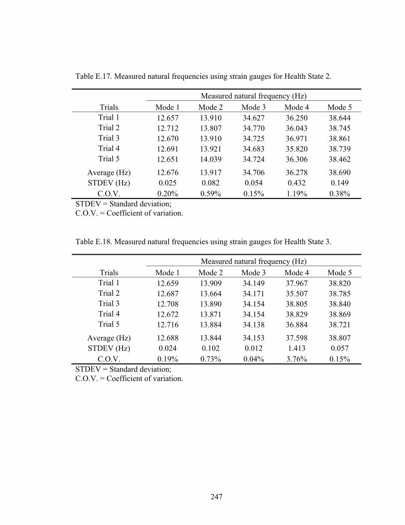
247
Table E.18. Measured natural frequencies using strain gauges for Health State 3.
Trials
Measured natural frequency (Hz)
Mode 1 Mode 2 Mode 3 Mode 4 Mode 5 Trial 1 12.659 13.909 34.149 37.967 38.820 Trial 2 12.687 13.664 34.171 35.507 38.785 Trial 3 12.708 13.890 34.154 38.805 38.840 Trial 4 12.672 13.871 34.154 38.829 38.869 Trial 5 12.716 13.884 34.138 36.884 38.721
Average (Hz) 12.688 13.844 34.153 37.598 38.807 STDEV (Hz) 0.024 0.102 0.012 1.413 0.057
C.O.V. 0.19% 0.73% 0.04% 3.76% 0.15% STDEV = Standard deviation; C.O.V. = Coefficient of variation.
Table E.17. Measured natural frequencies using strain gauges for Health State 2.
Trials
Measured natural frequency (Hz)
Mode 1 Mode 2 Mode 3 Mode 4 Mode 5 Trial 1 12.657 13.910 34.627 36.250 38.644 Trial 2 12.712 13.807 34.770 36.043 38.745 Trial 3 12.670 13.910 34.725 36.971 38.861 Trial 4 12.691 13.921 34.683 35.820 38.739 Trial 5 12.651 14.039 34.724 36.306 38.462
Average (Hz) 12.676 13.917 34.706 36.278 38.690 STDEV (Hz) 0.025 0.082 0.054 0.432 0.149
C.O.V. 0.20% 0.59% 0.15% 1.19% 0.38% STDEV = Standard deviation; C.O.V. = Coefficient of variation.
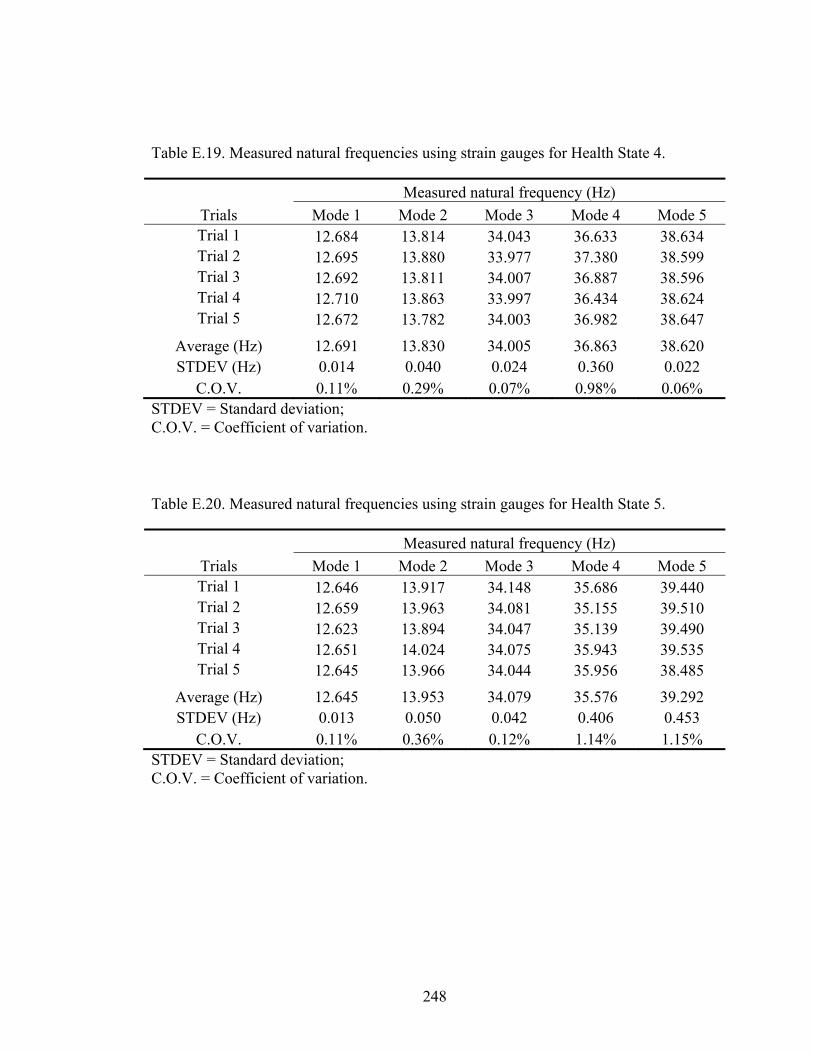
248
Table E.20. Measured natural frequencies using strain gauges for Health State 5.
Trials
Measured natural frequency (Hz)
Mode 1 Mode 2 Mode 3 Mode 4 Mode 5 Trial 1 12.646 13.917 34.148 35.686 39.440 Trial 2 12.659 13.963 34.081 35.155 39.510 Trial 3 12.623 13.894 34.047 35.139 39.490 Trial 4 12.651 14.024 34.075 35.943 39.535 Trial 5 12.645 13.966 34.044 35.956 38.485
Average (Hz) 12.645 13.953 34.079 35.576 39.292 STDEV (Hz) 0.013 0.050 0.042 0.406 0.453
C.O.V. 0.11% 0.36% 0.12% 1.14% 1.15% STDEV = Standard deviation; C.O.V. = Coefficient of variation.
Table E.19. Measured natural frequencies using strain gauges for Health State 4.
Trials
Measured natural frequency (Hz)
Mode 1 Mode 2 Mode 3 Mode 4 Mode 5 Trial 1 12.684 13.814 34.043 36.633 38.634 Trial 2 12.695 13.880 33.977 37.380 38.599 Trial 3 12.692 13.811 34.007 36.887 38.596 Trial 4 12.710 13.863 33.997 36.434 38.624 Trial 5 12.672 13.782 34.003 36.982 38.647
Average (Hz) 12.691 13.830 34.005 36.863 38.620 STDEV (Hz) 0.014 0.040 0.024 0.360 0.022
C.O.V. 0.11% 0.29% 0.07% 0.98% 0.06% STDEV = Standard deviation; C.O.V. = Coefficient of variation.
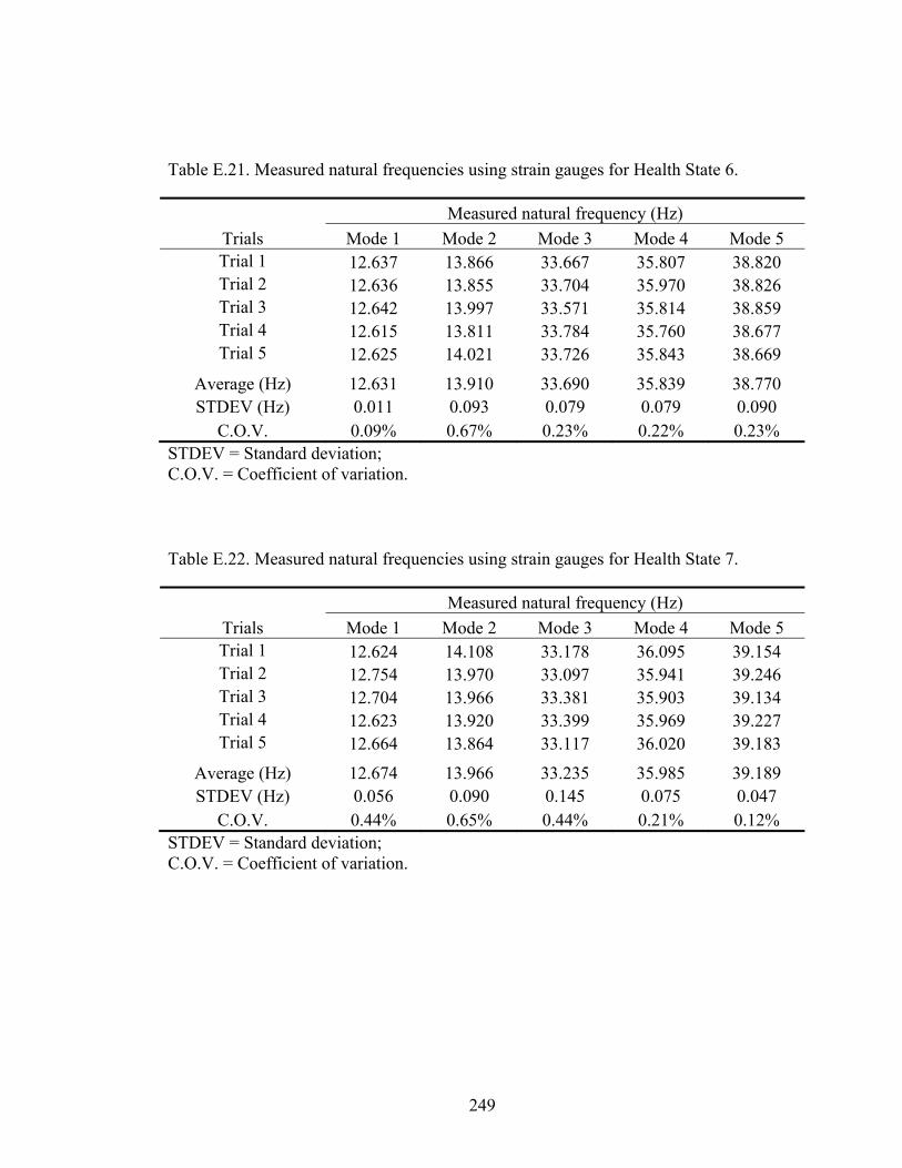
249
Table E.22. Measured natural frequencies using strain gauges for Health State 7.
Trials
Measured natural frequency (Hz)
Mode 1 Mode 2 Mode 3 Mode 4 Mode 5 Trial 1 12.624 14.108 33.178 36.095 39.154 Trial 2 12.754 13.970 33.097 35.941 39.246 Trial 3 12.704 13.966 33.381 35.903 39.134 Trial 4 12.623 13.920 33.399 35.969 39.227 Trial 5 12.664 13.864 33.117 36.020 39.183
Average (Hz) 12.674 13.966 33.235 35.985 39.189 STDEV (Hz) 0.056 0.090 0.145 0.075 0.047
C.O.V. 0.44% 0.65% 0.44% 0.21% 0.12% STDEV = Standard deviation; C.O.V. = Coefficient of variation.
Table E.21. Measured natural frequencies using strain gauges for Health State 6.
Trials
Measured natural frequency (Hz)
Mode 1 Mode 2 Mode 3 Mode 4 Mode 5 Trial 1 12.637 13.866 33.667 35.807 38.820 Trial 2 12.636 13.855 33.704 35.970 38.826 Trial 3 12.642 13.997 33.571 35.814 38.859 Trial 4 12.615 13.811 33.784 35.760 38.677 Trial 5 12.625 14.021 33.726 35.843 38.669
Average (Hz) 12.631 13.910 33.690 35.839 38.770 STDEV (Hz) 0.011 0.093 0.079 0.079 0.090
C.O.V. 0.09% 0.67% 0.23% 0.22% 0.23% STDEV = Standard deviation; C.O.V. = Coefficient of variation.
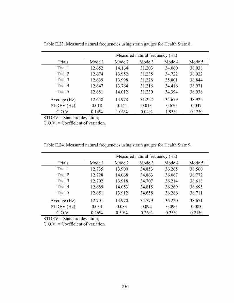
250
Table E.24. Measured natural frequencies using strain gauges for Health State 9.
Trials
Measured natural frequency (Hz)
Mode 1 Mode 2 Mode 3 Mode 4 Mode 5 Trial 1 12.735 13.900 34.853 36.265 38.560 Trial 2 12.728 14.068 34.863 36.067 38.772 Trial 3 12.702 13.918 34.707 36.214 38.618 Trial 4 12.689 14.053 34.815 36.269 38.695 Trial 5 12.651 13.912 34.658 36.286 38.711
Average (Hz) 12.701 13.970 34.779 36.220 38.671 STDEV (Hz) 0.034 0.083 0.092 0.090 0.083
C.O.V. 0.26% 0.59% 0.26% 0.25% 0.21% STDEV = Standard deviation; C.O.V. = Coefficient of variation.
Table E.23. Measured natural frequencies using strain gauges for Health State 8.
Trials
Measured natural frequency (Hz)
Mode 1 Mode 2 Mode 3 Mode 4 Mode 5 Trial 1 12.652 14.164 31.203 34.060 38.938 Trial 2 12.674 13.952 31.235 34.722 38.922 Trial 3 12.639 13.998 31.228 35.801 38.844 Trial 4 12.647 13.764 31.216 34.416 38.971 Trial 5 12.681 14.012 31.230 34.394 38.938
Average (Hz) 12.658 13.978 31.222 34.679 38.922 STDEV (Hz) 0.018 0.144 0.013 0.670 0.047
C.O.V. 0.14% 1.03% 0.04% 1.93% 0.12% STDEV = Standard deviation; C.O.V. = Coefficient of variation.

251
Table E.26. Measured natural frequencies using strain gauges for Health State 11.
Trials
Measured natural frequency (Hz)
Mode 1 Mode 2 Mode 3 Mode 4 Mode 5 Trial 1 12.628 13.863 34.269 35.974 39.103 Trial 2 12.671 14.089 34.177 36.041 39.173 Trial 3 12.645 13.846 34.266 36.074 39.215 Trial 4 12.659 13.805 34.123 35.996 39.207 Trial 5 12.731 13.985 34.248 36.206 39.122
Average (Hz) 12.667 13.917 34.216 36.058 39.164 STDEV (Hz) 0.040 0.117 0.064 0.091 0.050
C.O.V. 0.31% 0.84% 0.19% 0.25% 0.13% STDEV = Standard deviation; C.O.V. = Coefficient of variation.
Table E.25. Measured natural frequencies using strain gauges for Health State 10.
Trials
Measured natural frequency (Hz)
Mode 1 Mode 2 Mode 3 Mode 4 Mode 5 Trial 1 12.698 14.154 34.443 36.410 38.656 Trial 2 12.642 13.809 34.418 36.717 38.870 Trial 3 12.695 14.044 34.619 37.271 39.281 Trial 4 12.690 13.822 34.587 36.574 39.161 Trial 5 12.645 14.190 34.608 36.027 39.127
Average (Hz) 12.674 14.004 34.535 36.600 39.019 STDEV (Hz) 0.028 0.180 0.096 0.455 0.253
C.O.V. 0.22% 1.29% 0.28% 1.24% 0.65% STDEV = Standard deviation; C.O.V. = Coefficient of variation.

252
Table E.28. Measured natural frequencies using strain gauges for Health State 13.
Trials
Measured natural frequency (Hz)
Mode 1 Mode 2 Mode 3 Mode 4 Mode 5 Trial 1 12.722 14.749 33.983 36.053 38.711 Trial 2 12.725 14.569 33.845 36.203 38.905 Trial 3 12.757 14.302 33.805 36.114 38.635 Trial 4 12.773 14.919 34.032 36.192 38.685 Trial 5 12.721 14.334 33.644 36.163 38.541
Average (Hz) 12.740 14.575 33.862 36.145 38.695 STDEV (Hz) 0.024 0.265 0.154 0.062 0.134
C.O.V. 0.19% 1.82% 0.45% 0.17% 0.35% STDEV = Standard deviation; C.O.V. = Coefficient of variation.
Table E.27. Measured natural frequencies using strain gauges for Health State 12.
Trials
Measured natural frequency (Hz)
Mode 1 Mode 2 Mode 3 Mode 4 Mode 5 Trial 1 12.717 14.003 34.361 36.266 39.197 Trial 2 12.679 14.001 34.253 36.031 39.224 Trial 3 12.681 14.022 34.391 36.121 39.247 Trial 4 12.717 14.129 34.361 36.192 39.372 Trial 5 12.646 13.923 34.200 36.249 39.217
Average (Hz) 12.688 14.016 34.313 36.172 39.251 STDEV (Hz) 0.030 0.074 0.082 0.097 0.070
C.O.V. 0.24% 0.53% 0.24% 0.27% 0.18% STDEV = Standard deviation; C.O.V. = Coefficient of variation.

253
Table E.30. Measured natural frequencies using strain gauges for Health State 15.
Trials
Measured natural frequency (Hz)
Mode 1 Mode 2 Mode 3 Mode 4 Mode 5 Trial 1 12.815 13.970 34.220 36.229 38.705 Trial 2 12.756 15.158 34.327 36.199 38.730 Trial 3 12.756 14.426 34.202 36.147 38.545 Trial 4 12.762 14.739 34.232 36.419 38.639 Trial 5 12.761 14.292 33.976 36.098 38.720
Average (Hz) 12.770 14.517 34.191 36.218 38.668 STDEV (Hz) 0.025 0.452 0.130 0.123 0.077
C.O.V. 0.20% 3.11% 0.38% 0.34% 0.20% STDEV = Standard deviation; C.O.V. = Coefficient of variation.
Table E.29. Measured natural frequencies using strain gauges for Health State 14.
Trials
Measured natural frequency (Hz)
Mode 1 Mode 2 Mode 3 Mode 4 Mode 5 Trial 1 12.739 14.320 34.317 36.200 38.876 Trial 2 12.811 14.495 34.206 36.225 38.758 Trial 3 12.840 13.998 33.879 36.212 38.778 Trial 4 12.750 14.092 34.154 36.165 38.741 Trial 5 12.818 14.655 34.059 36.199 38.629
Average (Hz) 12.792 14.312 34.123 36.200 38.757 STDEV (Hz) 0.045 0.273 0.165 0.022 0.088
C.O.V. 0.35% 1.91% 0.48% 0.06% 0.23% STDEV = Standard deviation; C.O.V. = Coefficient of variation.

254
Table E.32. Measured natural frequencies using strain gauges for Health State 17.
Trials
Measured natural frequency (Hz)
Mode 1 Mode 2 Mode 3 Mode 4 Mode 5 Trial 1 12.731 14.353 34.463 36.267 38.881 Trial 2 12.719 14.044 34.091 36.180 38.567 Trial 3 12.710 14.229 34.072 36.179 38.827 Trial 4 12.734 14.470 34.505 36.336 38.755 Trial 5 12.769 14.578 34.174 36.336 38.937
Average (Hz) 12.733 14.335 34.261 36.260 38.793 STDEV (Hz) 0.022 0.208 0.208 0.079 0.143
C.O.V. 0.17% 1.45% 0.61% 0.22% 0.37% STDEV = Standard deviation; C.O.V. = Coefficient of variation.
Table E.31. Measured natural frequencies using strain gauges for Health State 16.
Trials
Measured natural frequency (Hz)
Mode 1 Mode 2 Mode 3 Mode 4 Mode 5 Trial 1 12.717 14.484 34.423 36.576 39.077 Trial 2 12.690 14.612 34.246 36.375 38.860 Trial 3 12.751 14.582 34.393 36.537 39.052 Trial 4 12.713 15.027 34.169 36.404 38.992 Trial 5 12.729 15.174 34.309 36.381 39.038
Average (Hz) 12.720 14.776 34.308 36.455 39.004 STDEV (Hz) 0.022 0.305 0.104 0.095 0.086
C.O.V. 0.18% 2.06% 0.30% 0.26% 0.22% STDEV = Standard deviation; C.O.V. = Coefficient of variation.
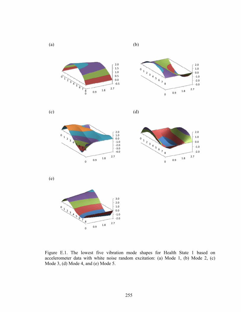
255
Figure E.1. The lowest five vibration mode shapes for Health State 1 based onaccelerometer data with white noise random excitation: (a) Mode 1, (b) Mode 2, (c)Mode 3, (d) Mode 4, and (e) Mode 5.
(a) (b)
(c) (d)
(e)
00.9
1.82.7
‐0.5
0.0
0.5
1.0
1.5
2.0
01
23
45
67
80
0.91.8
2.7
‐3.0
‐2.0
‐1.0
0.0
1.0
2.0
01
23
45
67
8
00.9
1.82.7
‐4.0‐3.0‐2.0‐1.00.01.02.0
01
23
45
67
8
00.9
1.82.7
‐2.0
‐1.0
0.0
1.0
2.0
01
23
45
67
8
00.9
1.82.7
‐2.0
‐1.0
0.0
1.0
2.0
3.0
01
23
45
67
8

256
0.0
0.5
1.0
1.5
2.0
State 1 State 14 State 15 State 16 State 17
Figure E.2. Comparison of the first mode shape averaged from five repeated tests fordifferent health states using accelerometer data with white noise random excitation.
Girder line 1 Girder line 2 Girder line 3 Girder line 4
0.0
0.5
1.0
1.5
2.0
State 1 State 2 State 3 State 4 State 5
0.0
0.5
1.0
1.5
2.0
State 1 State 6 State 7 State 8 State 9
0.0
0.5
1.0
1.5
2.0
State 1 State 10 State 11 State 12 State 13
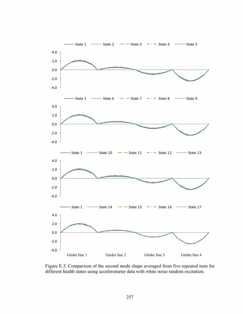
257
‐4.0
‐2.0
0.0
2.0
4.0
State 1 State 14 State 15 State 16 State 17
Figure E.3. Comparison of the second mode shape averaged from five repeated tests fordifferent health states using accelerometer data with white noise random excitation.
Girder line 1 Girder line 2 Girder line 3 Girder line 4
‐4.0
‐2.0
0.0
2.0
4.0
State 1 State 2 State 3 State 4 State 5
‐4.0
‐2.0
0.0
2.0
4.0
State 1 State 6 State 7 State 8 State 9
‐4.0
‐2.0
0.0
2.0
4.0
State 1 State 10 State 11 State 12 State 13

258
‐4.0
‐2.0
0.0
2.0
4.0
State 1 State 14 State 15 State 16 State 17
Figure E.4. Comparison of the third mode shape averaged from five repeated tests fordifferent health states using accelerometer data with white noise random excitation.
Girder line 1 Girder line 2 Girder line 3 Girder line 4
‐4.0
‐2.0
0.0
2.0
4.0
State 1 State 2 State 3 State 4 State 5
‐4.0
‐2.0
0.0
2.0
4.0
State 1 State 6 State 7 State 8 State 9
‐4.0
‐2.0
0.0
2.0
4.0
State 1 State 10 State 11 State 12 State 13
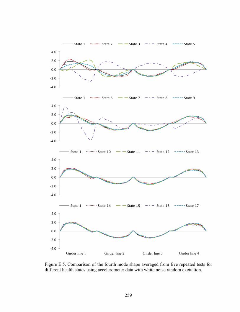
259
‐4.0
‐2.0
0.0
2.0
4.0
State 1 State 14 State 15 State 16 State 17
Figure E.5. Comparison of the fourth mode shape averaged from five repeated tests fordifferent health states using accelerometer data with white noise random excitation.
Girder line 1 Girder line 2 Girder line 3 Girder line 4
‐4.0
‐2.0
0.0
2.0
4.0
State 1 State 2 State 3 State 4 State 5
‐4.0
‐2.0
0.0
2.0
4.0
State 1 State 6 State 7 State 8 State 9
‐4.0
‐2.0
0.0
2.0
4.0
State 1 State 10 State 11 State 12 State 13
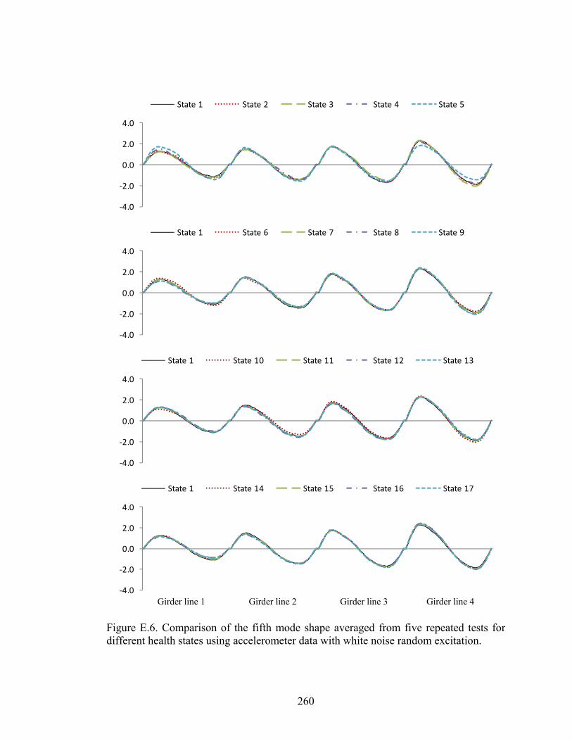
260
‐4.0
‐2.0
0.0
2.0
4.0
State 1 State 14 State 15 State 16 State 17
Figure E.6. Comparison of the fifth mode shape averaged from five repeated tests fordifferent health states using accelerometer data with white noise random excitation.
Girder line 1 Girder line 2 Girder line 3 Girder line 4
‐4.0
‐2.0
0.0
2.0
4.0
State 1 State 2 State 3 State 4 State 5
‐4.0
‐2.0
0.0
2.0
4.0
State 1 State 6 State 7 State 8 State 9
‐4.0
‐2.0
0.0
2.0
4.0
State 1 State 10 State 11 State 12 State 13
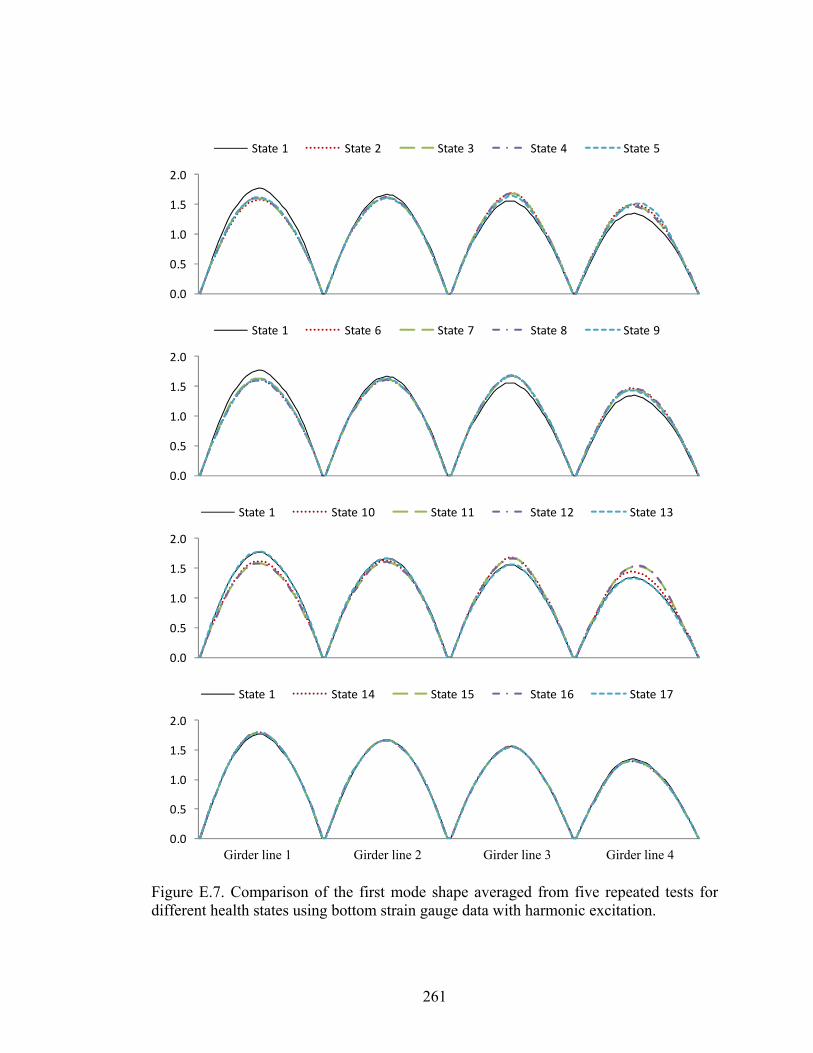
261
0.0
0.5
1.0
1.5
2.0
State 1 State 14 State 15 State 16 State 17
Figure E.7. Comparison of the first mode shape averaged from five repeated tests fordifferent health states using bottom strain gauge data with harmonic excitation.
Girder line 1 Girder line 2 Girder line 3 Girder line 4
0.0
0.5
1.0
1.5
2.0
State 1 State 2 State 3 State 4 State 5
0.0
0.5
1.0
1.5
2.0
State 1 State 6 State 7 State 8 State 9
0.0
0.5
1.0
1.5
2.0
State 1 State 10 State 11 State 12 State 13

262
‐4.0
‐2.0
0.0
2.0
4.0
State 1 State 14 State 15 State 16 State 17
Figure E.8. Comparison of the second mode shape averaged from five repeated tests fordifferent health states using bottom strain gauge data with harmonic excitation.
Girder line 1 Girder line 2 Girder line 3 Girder line 4
‐4.0
‐2.0
0.0
2.0
4.0
State 1 State 2 State 3 State 4 State 5
‐4.0
‐2.0
0.0
2.0
4.0
State 1 State 6 State 7 State 8 State 9
‐4.0
‐2.0
0.0
2.0
4.0
State 1 State 10 State 11 State 12 State 13

263
0.0
0.5
1.0
1.5
2.0
State 1 State 14 State 15 State 16 State 17
Figure E.9. Comparison of the first mode shape averaged from five repeated tests fordifferent health states using bottom strain gauge data with white noise randomexcitation.
Girder line 1 Girder line 2 Girder line 3 Girder line 4
0.0
0.5
1.0
1.5
2.0
State 1 State 2 State 3 State 4 State 5
0.0
0.5
1.0
1.5
2.0
State 1 State 6 State 7 State 8 State 9
0.0
0.5
1.0
1.5
2.0
State 1 State 10 State 11 State 12 State 13
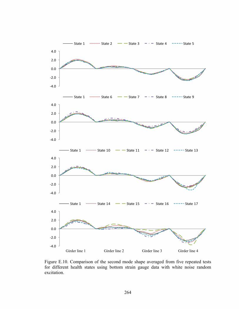
264
‐4.0
‐2.0
0.0
2.0
4.0
State 1 State 14 State 15 State 16 State 17
Figure E.10. Comparison of the second mode shape averaged from five repeated testsfor different health states using bottom strain gauge data with white noise randomexcitation.
Girder line 1 Girder line 2 Girder line 3 Girder line 4
‐4.0
‐2.0
0.0
2.0
4.0
State 1 State 2 State 3 State 4 State 5
‐4.0
‐2.0
0.0
2.0
4.0
State 1 State 6 State 7 State 8 State 9
‐4.0
‐2.0
0.0
2.0
4.0
State 1 State 10 State 11 State 12 State 13
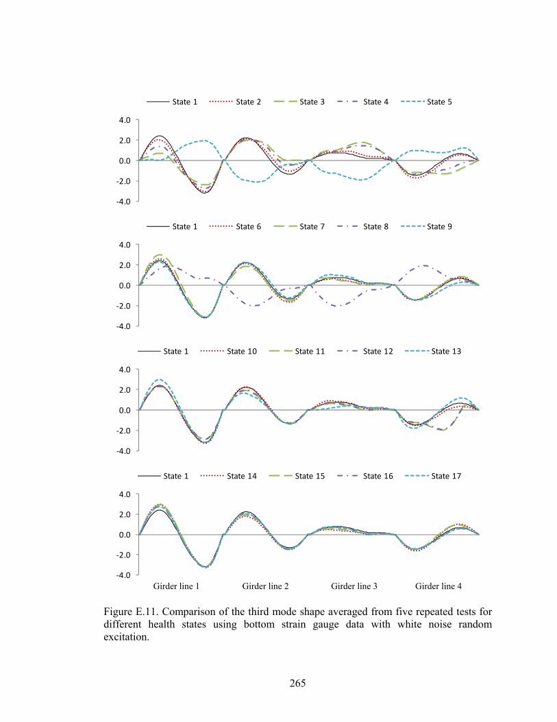
265
‐4.0
‐2.0
0.0
2.0
4.0
State 1 State 14 State 15 State 16 State 17
Figure E.11. Comparison of the third mode shape averaged from five repeated tests fordifferent health states using bottom strain gauge data with white noise randomexcitation.
Girder line 1 Girder line 2 Girder line 3 Girder line 4
‐4.0
‐2.0
0.0
2.0
4.0
State 1 State 2 State 3 State 4 State 5
‐4.0
‐2.0
0.0
2.0
4.0
State 1 State 6 State 7 State 8 State 9
‐4.0
‐2.0
0.0
2.0
4.0
State 1 State 10 State 11 State 12 State 13
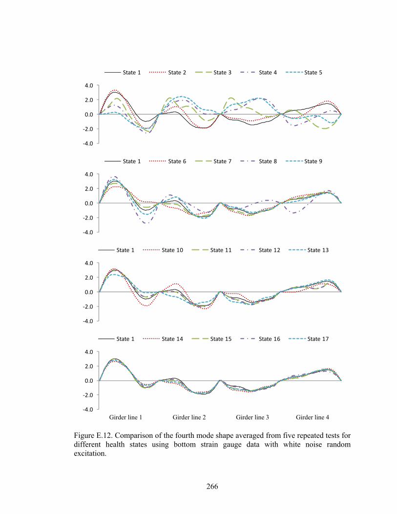
266
‐4.0
‐2.0
0.0
2.0
4.0
State 1 State 14 State 15 State 16 State 17
Figure E.12. Comparison of the fourth mode shape averaged from five repeated tests fordifferent health states using bottom strain gauge data with white noise randomexcitation.
Girder line 1 Girder line 2 Girder line 3 Girder line 4
‐4.0
‐2.0
0.0
2.0
4.0
State 1 State 2 State 3 State 4 State 5
‐4.0
‐2.0
0.0
2.0
4.0
State 1 State 6 State 7 State 8 State 9
‐4.0
‐2.0
0.0
2.0
4.0
State 1 State 10 State 11 State 12 State 13
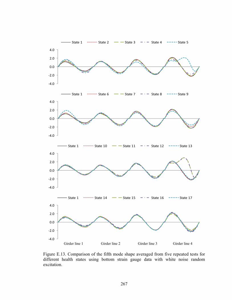
267
‐4.0
‐2.0
0.0
2.0
4.0
State 1 State 14 State 15 State 16 State 17
Figure E.13. Comparison of the fifth mode shape averaged from five repeated tests fordifferent health states using bottom strain gauge data with white noise randomexcitation.
Girder line 1 Girder line 2 Girder line 3 Girder line 4
‐4.0
‐2.0
0.0
2.0
4.0
State 1 State 2 State 3 State 4 State 5
‐4.0
‐2.0
0.0
2.0
4.0
State 1 State 6 State 7 State 8 State 9
‐4.0
‐2.0
0.0
2.0
4.0
State 1 State 10 State 11 State 12 State 13

268
APPENDIX F. ADDITIONAL INFORMATION FOR THE
FE MODEL
This Appendix presents additional explanation of results generated using the FE model,
as described in Chapter 5. Specifically, Figure F.1 presents exactly the same results as
shown in Fig. 5.10. To better understand the relationship between the area of mode
shape change and the relative flexural stiffness, however, a linear scale was used in this
figure while a logarithmic scale was used in Fig. 5.10.
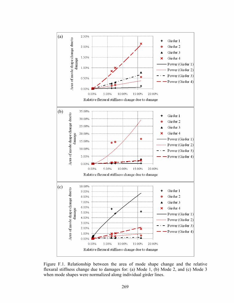
269
Figure F.1. Relationship between the area of mode shape change and the relativeflexural stiffness change due to damages for: (a) Mode 1, (b) Mode 2, and (c) Mode 3when mode shapes were normalized along individual girder lines.
(b)
(c)
(a)

270
APPENDIX G. ADDITIONAL INFORMATION FOR
DISTRIBUTION OF THE AREA OF MODE SHAPE
CHANGE
This appendix presents additional information for the distribution of the area of mode
shape change when there is no change in condition, as described in Section 6.2.2.
Figures G.1 to G.5 present comparisons of the actual cumulative probability
distributions and the assumed Normal and Log-Normal distributions of Δ for Test
Protocols 9 to 28, which are similar to results presented in Figs. 6.1 and 6.2.
Figures G.6 to G.15 present comparison of the probability density between the actual
distribution and the assumed Normal and Log-Normal distributions of Δ , for Test
Protocols 9 to 28, which supply additional information for Figs. 6.3 to 6.6.
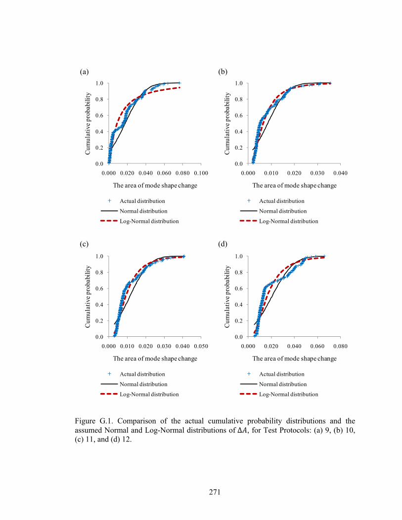
271
Figure G.1. Comparison of the actual cumulative probability distributions and theassumed Normal and Log-Normal distributions of Δ , for Test Protocols: (a) 9, (b) 10,(c) 11, and (d) 12.
(a) (b)
(c) (d)
0.0
0.2
0.4
0.6
0.8
1.0
0.000 0.020 0.040 0.060 0.080 0.100
Cum
ulat
ive
prob
abili
ty
The area of mode shape change
Actual distribution
Normal distribution
Log-Normal distribution
0.0
0.2
0.4
0.6
0.8
1.0
0.000 0.010 0.020 0.030 0.040
Cum
ulat
ive
prob
abili
ty
The area of mode shape change
Actual distribution
Normal distribution
Log-Normal distribution
0.0
0.2
0.4
0.6
0.8
1.0
0.000 0.010 0.020 0.030 0.040 0.050
Cum
ulat
ive
prob
abili
ty
The area of mode shape change
Actual distribution
Normal distribution
Log-Normal distribution
0.0
0.2
0.4
0.6
0.8
1.0
0.000 0.020 0.040 0.060 0.080
Cum
ulat
ive
prob
abili
ty
The area of mode shape change
Actual distribution
Normal distribution
Log-Normal distribution
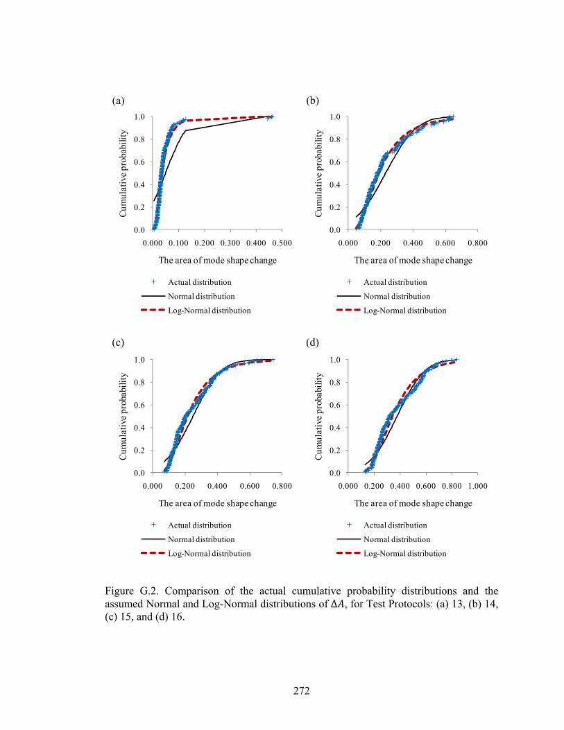
272
Figure G.2. Comparison of the actual cumulative probability distributions and theassumed Normal and Log-Normal distributions of Δ , for Test Protocols: (a) 13, (b) 14,(c) 15, and (d) 16.
(a) (b)
(c) (d)
0.0
0.2
0.4
0.6
0.8
1.0
0.000 0.100 0.200 0.300 0.400 0.500
Cum
ulat
ive
prob
abili
ty
The area of mode shape change
Actual distribution
Normal distribution
Log-Normal distribution
0.0
0.2
0.4
0.6
0.8
1.0
0.000 0.200 0.400 0.600 0.800
Cum
ulat
ive
prob
abili
ty
The area of mode shape change
Actual distribution
Normal distribution
Log-Normal distribution
0.0
0.2
0.4
0.6
0.8
1.0
0.000 0.200 0.400 0.600 0.800
Cum
ulat
ive
prob
abili
ty
The area of mode shape change
Actual distribution
Normal distribution
Log-Normal distribution
0.0
0.2
0.4
0.6
0.8
1.0
0.000 0.200 0.400 0.600 0.800 1.000
Cum
ulat
ive
prob
abili
ty
The area of mode shape change
Actual distribution
Normal distribution
Log-Normal distribution

273
Figure G.3. Comparison of the actual cumulative probability distributions and theassumed Normal and Log-Normal distributions of Δ , for Test Protocols: (a) 17, (b) 18,(c) 19, and (d) 20.
(a) (b)
(c) (d)
0.0
0.2
0.4
0.6
0.8
1.0
0.000 0.020 0.040 0.060 0.080 0.100
Cum
ulat
ive
prob
abili
ty
The area of mode shape change
Actual distribution
Normal distribution
Log-Normal distribution
0.0
0.2
0.4
0.6
0.8
1.0
0.000 0.100 0.200 0.300
Cum
ulat
ive
prob
abili
ty
The area of mode shape change
Actual distribution
Normal distribution
Log-Normal distribution
0.0
0.2
0.4
0.6
0.8
1.0
0.000 0.100 0.200 0.300
Cum
ulat
ive
prob
abili
ty
The area of mode shape change
Actual distribution
Normal distribution
Log-Normal distribution
0.0
0.2
0.4
0.6
0.8
1.0
0.000 0.100 0.200 0.300 0.400 0.500
Cum
ulat
ive
prob
abili
ty
The area of mode shape change
Actual distribution
Normal distribution
Log-Normal distribution
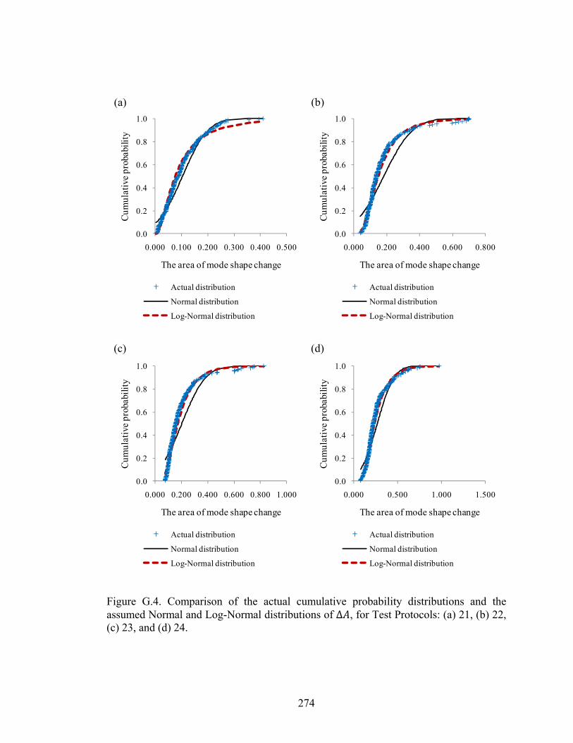
274
Figure G.4. Comparison of the actual cumulative probability distributions and theassumed Normal and Log-Normal distributions of Δ , for Test Protocols: (a) 21, (b) 22,(c) 23, and (d) 24.
(a) (b)
(c) (d)
0.0
0.2
0.4
0.6
0.8
1.0
0.000 0.100 0.200 0.300 0.400 0.500
Cum
ulat
ive
prob
abili
ty
The area of mode shape change
Actual distribution
Normal distribution
Log-Normal distribution
0.0
0.2
0.4
0.6
0.8
1.0
0.000 0.200 0.400 0.600 0.800
Cum
ulat
ive
prob
abili
ty
The area of mode shape change
Actual distribution
Normal distribution
Log-Normal distribution
0.0
0.2
0.4
0.6
0.8
1.0
0.000 0.200 0.400 0.600 0.800 1.000
Cum
ulat
ive
prob
abili
ty
The area of mode shape change
Actual distribution
Normal distribution
Log-Normal distribution
0.0
0.2
0.4
0.6
0.8
1.0
0.000 0.500 1.000 1.500
Cum
ulat
ive
prob
abili
ty
The area of mode shape change
Actual distribution
Normal distribution
Log-Normal distribution
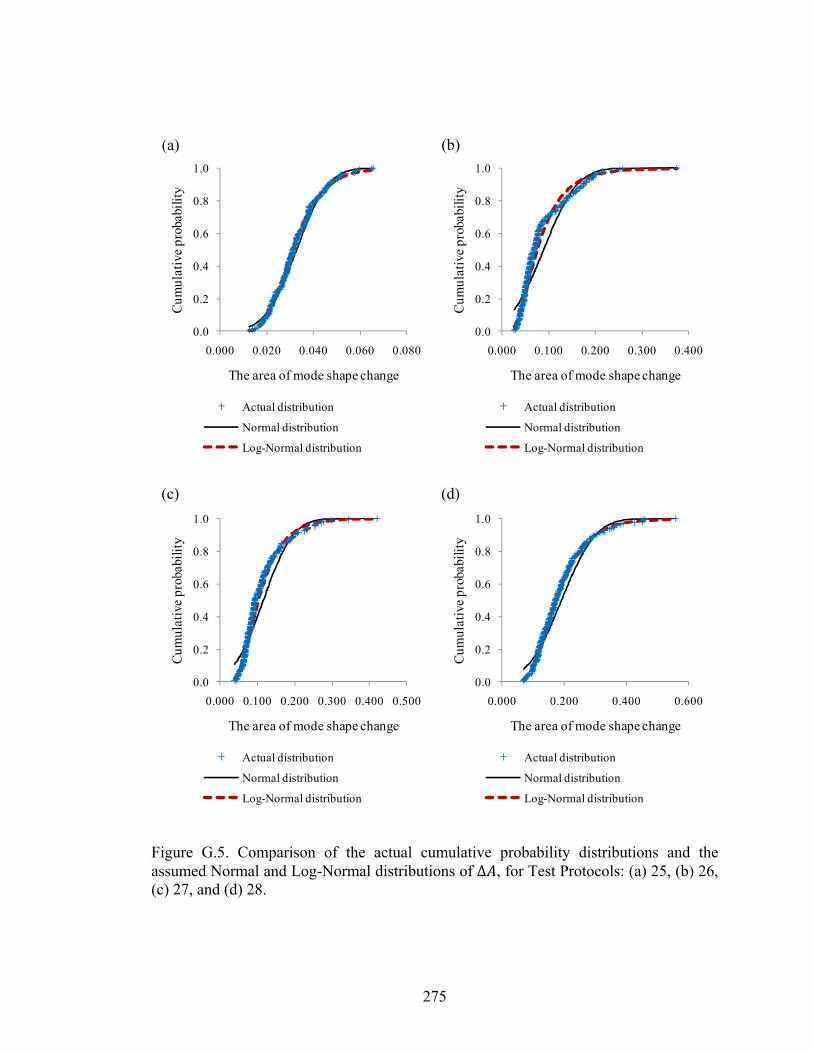
275
Figure G.5. Comparison of the actual cumulative probability distributions and theassumed Normal and Log-Normal distributions of Δ , for Test Protocols: (a) 25, (b) 26,(c) 27, and (d) 28.
(a) (b)
(c) (d)
0.0
0.2
0.4
0.6
0.8
1.0
0.000 0.020 0.040 0.060 0.080
Cum
ulat
ive
prob
abili
ty
The area of mode shape change
Actual distribution
Normal distribution
Log-Normal distribution
0.0
0.2
0.4
0.6
0.8
1.0
0.000 0.100 0.200 0.300 0.400
Cum
ulat
ive
prob
abili
ty
The area of mode shape change
Actual distribution
Normal distribution
Log-Normal distribution
0.0
0.2
0.4
0.6
0.8
1.0
0.000 0.100 0.200 0.300 0.400 0.500
Cum
ulat
ive
prob
abili
ty
The area of mode shape change
Actual distribution
Normal distribution
Log-Normal distribution
0.0
0.2
0.4
0.6
0.8
1.0
0.000 0.200 0.400 0.600
Cum
ulat
ive
prob
abili
ty
The area of mode shape change
Actual distribution
Normal distribution
Log-Normal distribution
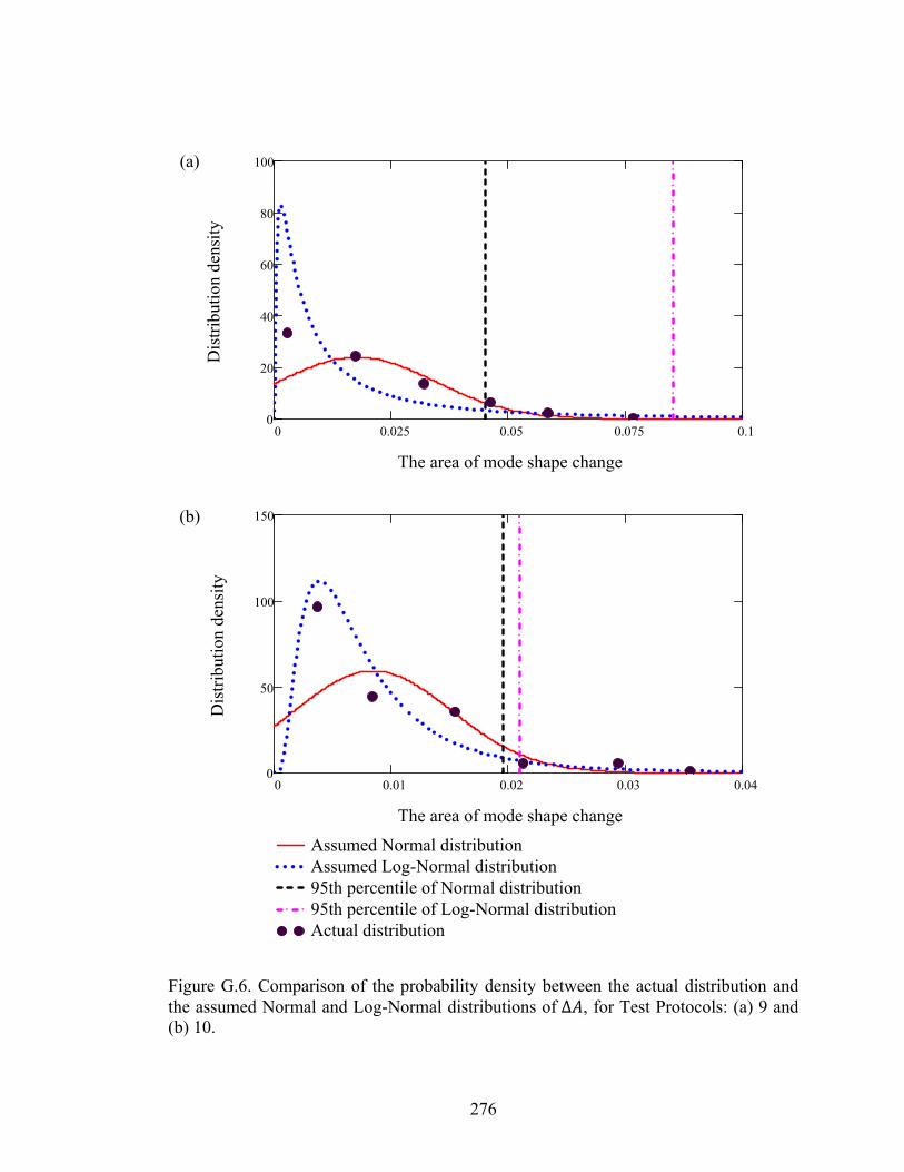
276
Figure G.6. Comparison of the probability density between the actual distribution andthe assumed Normal and Log-Normal distributions of Δ , for Test Protocols: (a) 9 and(b) 10.
(a)
(b)
0 0.025 0.05 0.075 0.10
20
40
60
80
100
The area of mode shape change
Dis
trib
utio
n de
nsit
y
0 0.01 0.02 0.03 0.040
50
100
150
Assumed Normal distributionAssumed Log-Normal distribution95th percentile of Normal distribution95th percentile of Log-Normal distributionActual distribution
The area of mode shape change
Dis
trib
utio
n de
nsit
y

277
Figure G.7. Comparison of the probability density between the actual distribution andthe assumed Normal and Log-Normal distributions of Δ , for Test Protocols: (a) 11 and(b) 12.
(a)
(b)
0 0.01 0.02 0.03 0.040
20
40
60
80
100
The area of mode shape change
Dis
trib
utio
n de
nsit
y
0 0.02 0.04 0.06 0.080
20
40
60
80
100
Assumed Normal distributionAssumed Log-Normal distribution95th percentile of Normal distribution95th percentile of Log-Normal distributionActual distribution
The area of mode shape change
Dis
trib
utio
n de
nsit
y

278
Figure G.8. Comparison of the probability density between the actual distribution andthe assumed Normal and Log-Normal distributions of Δ , for Test Protocols: (a) 13 and(b) 14.
(a)
(b)
0 0.2 0.4 0.6 0.80
2
4
6
Assumed Normal distributionAssumed Log-Normal distribution95th percentile of Normal distribution95th percentile of Log-Normal distributionActual distribution
The area of mode shape change
Dis
trib
utio
n de
nsit
y
0 0.125 0.25 0.375 0.50
10
20
30
The area of mode shape change
Dis
trib
utio
n de
nsit
y
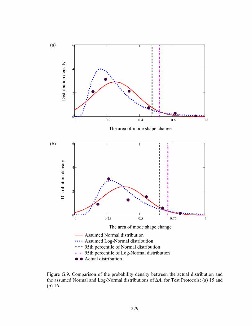
279
Figure G.9. Comparison of the probability density between the actual distribution andthe assumed Normal and Log-Normal distributions of Δ , for Test Protocols: (a) 15 and(b) 16.
(a)
(b)
0 0.2 0.4 0.6 0.80
2
4
6
The area of mode shape change
Dis
trib
utio
n de
nsit
y
0 0.25 0.5 0.75 10
2
4
6
Assumed Normal distributionAssumed Log-Normal distribution95th percentile of Normal distribution95th percentile of Log-Normal distributionActual distribution
The area of mode shape change
Dis
trib
utio
n de
nsit
y

280
Figure G.10. Comparison of the probability density between the actual distribution andthe assumed Normal and Log-Normal distributions of Δ , for Test Protocols: (a) 17 and(b) 18.
(a)
(b)
0 0.025 0.05 0.075 0.10
20
40
60
The area of mode shape change
Dis
trib
utio
n de
nsit
y
0 0.1 0.2 0.3 0.40
5
10
15
20
Assumed Normal distributionAssumed Log-Normal distribution95th percentile of Normal distribution95th percentile of Log-Normal distributionActual distribution
The area of mode shape change
Dis
trib
utio
n de
nsit
y
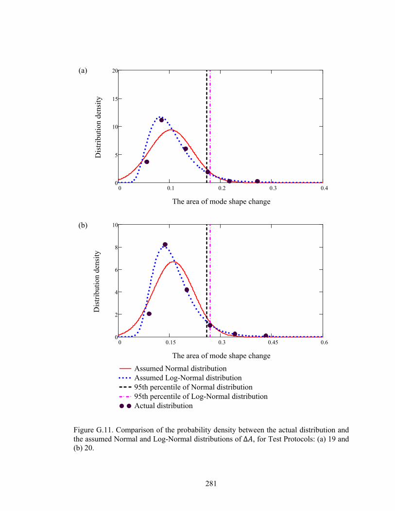
281
Figure G.11. Comparison of the probability density between the actual distribution andthe assumed Normal and Log-Normal distributions of Δ , for Test Protocols: (a) 19 and(b) 20.
(a)
(b)
0 0.1 0.2 0.3 0.40
5
10
15
20
The area of mode shape change
Dis
trib
utio
n de
nsit
y
0 0.15 0.3 0.45 0.60
2
4
6
8
10
Assumed Normal distributionAssumed Log-Normal distribution95th percentile of Normal distribution95th percentile of Log-Normal distributionActual distribution
The area of mode shape change
Dis
trib
utio
n de
nsit
y

282
Figure G.12. Comparison of the probability density between the actual distribution andthe assumed Normal and Log-Normal distributions of Δ , for Test Protocols: (a) 21 and(b) 22.
(a)
(b)
0 0.15 0.3 0.45 0.60
2
4
6
8
10
The area of mode shape change
Dis
trib
utio
n de
nsit
y
0 0.2 0.4 0.6 0.80
2
4
6
Assumed Normal distributionAssumed Log-Normal distribution95th percentile of Normal distribution95th percentile of Log-Normal distributionActual distribution
The area of mode shape change
Dis
trib
utio
n de
nsit
y
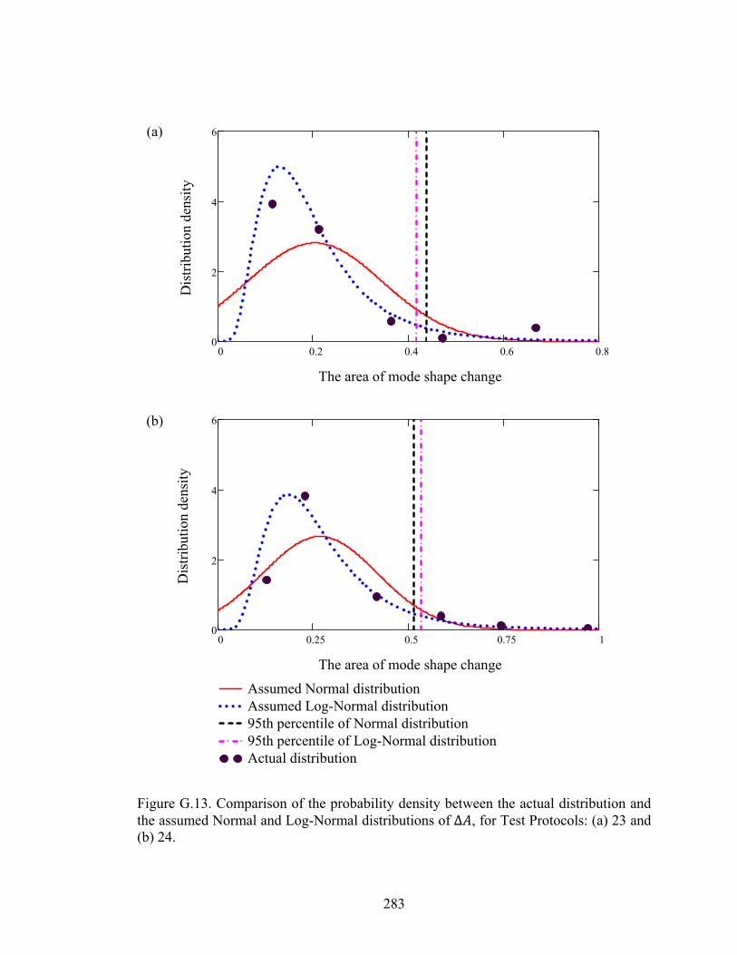
283
Figure G.13. Comparison of the probability density between the actual distribution andthe assumed Normal and Log-Normal distributions of Δ , for Test Protocols: (a) 23 and(b) 24.
(a)
(b)
0 0.2 0.4 0.6 0.80
2
4
6
The area of mode shape change
Dis
trib
utio
n de
nsit
y
0 0.25 0.5 0.75 10
2
4
6
Assumed Normal distributionAssumed Log-Normal distribution95th percentile of Normal distribution95th percentile of Log-Normal distributionActual distribution
The area of mode shape change
Dis
trib
utio
n de
nsit
y
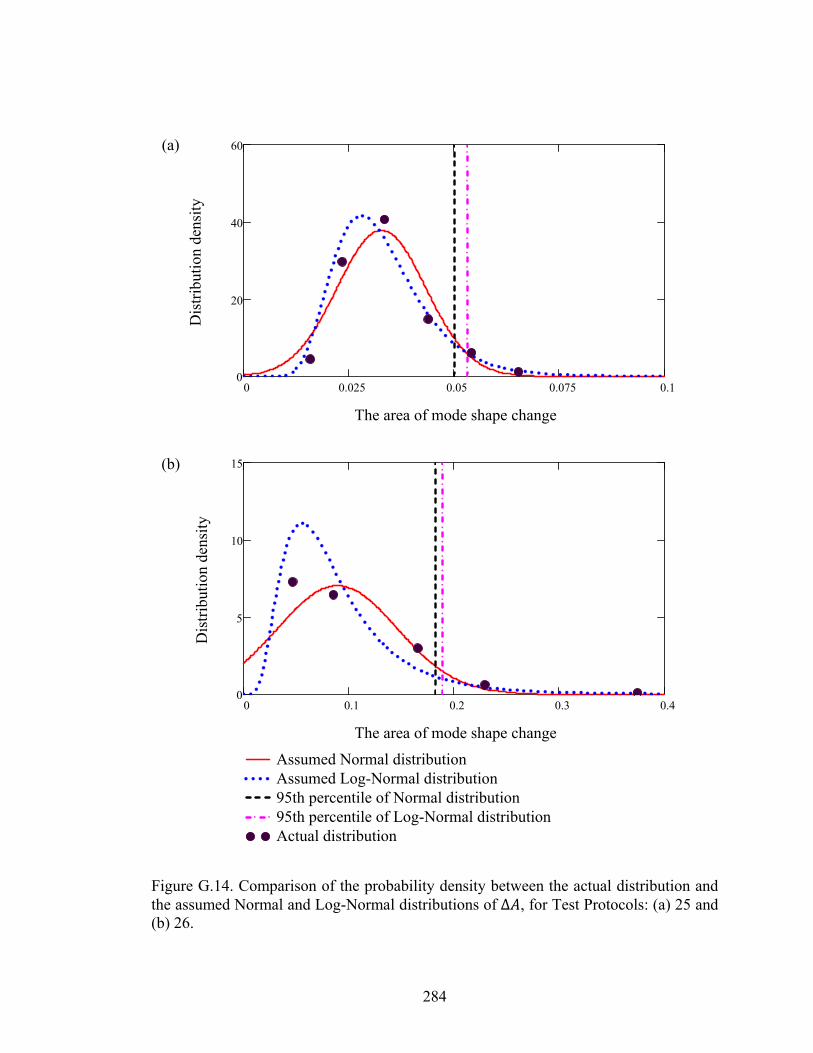
284
Figure G.14. Comparison of the probability density between the actual distribution andthe assumed Normal and Log-Normal distributions of Δ , for Test Protocols: (a) 25 and(b) 26.
(a)
(b)
0 0.025 0.05 0.075 0.10
20
40
60
The area of mode shape change
Dis
trib
utio
n de
nsit
y
0 0.1 0.2 0.3 0.40
5
10
15
Assumed Normal distributionAssumed Log-Normal distribution95th percentile of Normal distribution95th percentile of Log-Normal distributionActual distribution
The area of mode shape change
Dis
trib
utio
n de
nsit
y
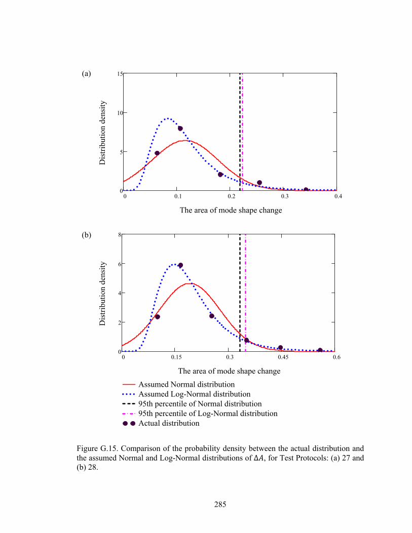
285
Figure G.15. Comparison of the probability density between the actual distribution andthe assumed Normal and Log-Normal distributions of Δ , for Test Protocols: (a) 27 and(b) 28.
(a)
(b)
0 0.1 0.2 0.3 0.40
5
10
15
The area of mode shape change
Dis
trib
utio
n de
nsit
y
0 0.15 0.3 0.45 0.60
2
4
6
8
Assumed Normal distributionAssumed Log-Normal distribution95th percentile of Normal distribution95th percentile of Log-Normal distributionActual distribution
The area of mode shape change
Dis
trib
utio
n de
nsit
y

286
APPENDIX H. ADDITIONAL INFORMATION FOR
DETECTION OF THE PRESENCE OF DAMAGE
This appendix presents additional information for detection of the presence of damage,
as described in Section 6.2.5, Section 6.2.6, and Section 6.2.7.
Tables H.1 to H.4 present the summary of area of change in the first mode shape due to
Damage Cases 4 to 26 for different test trials when Test Protocol 1 was used, which are
similar to the results listed in Table 6.7.
Tables H.5 to H.39 present the summary of area of change in the first mode shape due to
Damage Cases 1 to 26 for different test trials when Test Protocols 2 to 8 were used.
Figures H.1 to H.8 present comparisons of the assumed Normal distributions of the area
of mode shape change for the undamaged group of 170 pairs and the damaged group of
25 data pairs for Damage Cases 4 to 26, when Test Protocol 1 was used. The results in
these figures are similar to those presented in Fig. 6.7.
Figures H.9 to H.35 present the distribution with the assumed Normal distribution for
Damage Cases 1 to 26, when Test Protocols 2 to 4 were used.
Tables H.40 to H.43 present the probabilities that there was no change in condition
using the assumed Normal distributions (i.e., the probability that the Δ value obtained
when there was a change in the condition did not exceed those that obtained when there
was no change in condition), for Damage Cases 4 to 26 using all 28 Test Protocols,
which are similar to results listed in Table 6.8.
287
Tables H.44 to H.47 present the probabilities that there was no change in condition
using the assumed Log-Normal distributions (i.e., the probability that the Δ value
obtained when there was a change in the condition did not exceed those that obtained
when there was no change in condition), for Damage Cases 4 to 26 using all 28 Test
Protocols, which are similar to results listed in Table 6.9.
Tables H.48 to H.51 present the ratios of the area of the mode shape changes to the
corresponding threshold values, defined as the 95th percentile of assumed Log-Normal
distributions, as listed in Table 6.6, due to Damage Cases 4 to 26 for all 28 Test
Protocols, which supply additional information for Section 6.2.6.
Figures H.36 to H.42 present comparisons of mean Δ values from 25 data pairs for all
single damage cases to the 90% and 95% threshold values, when Test Protocols 2 to 8
were used, which are similar to the results presented in Fig. 6.9.
Figures H.43 to H.49 present ratios of area of mode shape change (the average of 25
values) to the 90% threshold values when Test Protocols 1 to 28 were used, which are
similar to results presented in Figs. 6.10 to 6.16 where the ratios were calculated using
95% threshold values.
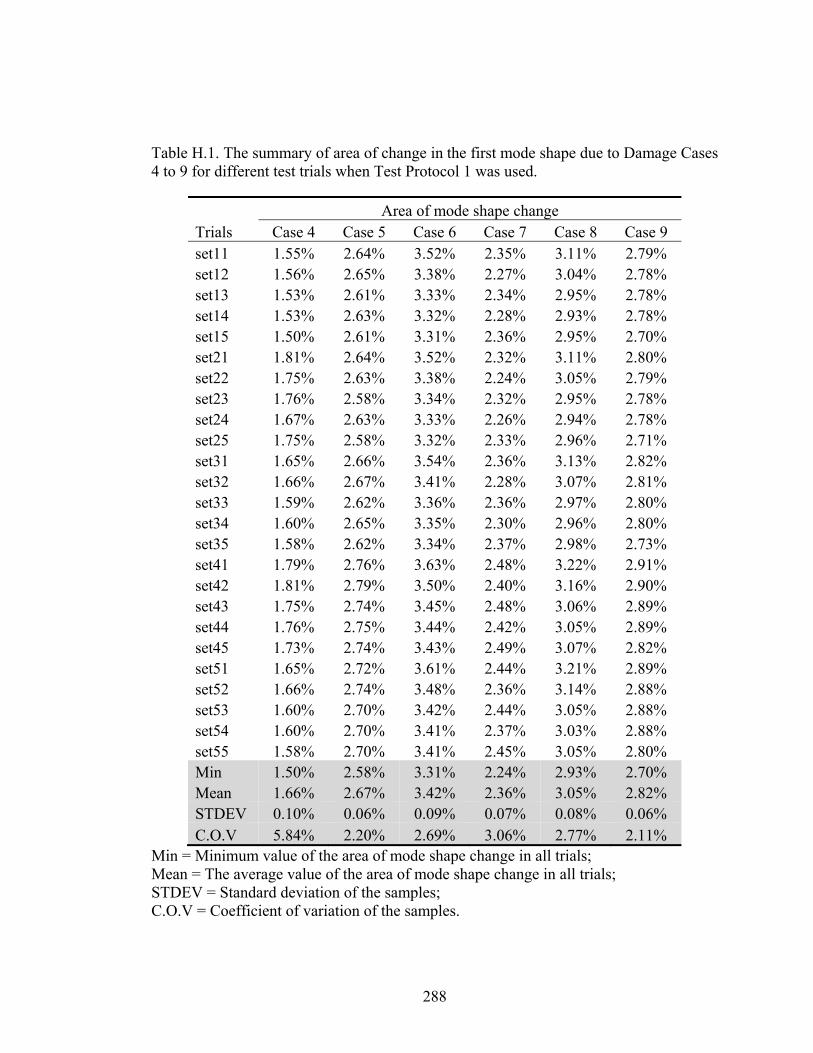
288
Table H.1. The summary of area of change in the first mode shape due to Damage Cases 4 to 9 for different test trials when Test Protocol 1 was used.
Area of mode shape change Trials Case 4 Case 5 Case 6 Case 7 Case 8 Case 9 set11 1.55% 2.64% 3.52% 2.35% 3.11% 2.79% set12 1.56% 2.65% 3.38% 2.27% 3.04% 2.78% set13 1.53% 2.61% 3.33% 2.34% 2.95% 2.78% set14 1.53% 2.63% 3.32% 2.28% 2.93% 2.78% set15 1.50% 2.61% 3.31% 2.36% 2.95% 2.70% set21 1.81% 2.64% 3.52% 2.32% 3.11% 2.80% set22 1.75% 2.63% 3.38% 2.24% 3.05% 2.79% set23 1.76% 2.58% 3.34% 2.32% 2.95% 2.78% set24 1.67% 2.63% 3.33% 2.26% 2.94% 2.78% set25 1.75% 2.58% 3.32% 2.33% 2.96% 2.71% set31 1.65% 2.66% 3.54% 2.36% 3.13% 2.82% set32 1.66% 2.67% 3.41% 2.28% 3.07% 2.81% set33 1.59% 2.62% 3.36% 2.36% 2.97% 2.80% set34 1.60% 2.65% 3.35% 2.30% 2.96% 2.80% set35 1.58% 2.62% 3.34% 2.37% 2.98% 2.73% set41 1.79% 2.76% 3.63% 2.48% 3.22% 2.91% set42 1.81% 2.79% 3.50% 2.40% 3.16% 2.90% set43 1.75% 2.74% 3.45% 2.48% 3.06% 2.89% set44 1.76% 2.75% 3.44% 2.42% 3.05% 2.89% set45 1.73% 2.74% 3.43% 2.49% 3.07% 2.82% set51 1.65% 2.72% 3.61% 2.44% 3.21% 2.89% set52 1.66% 2.74% 3.48% 2.36% 3.14% 2.88% set53 1.60% 2.70% 3.42% 2.44% 3.05% 2.88% set54 1.60% 2.70% 3.41% 2.37% 3.03% 2.88% set55 1.58% 2.70% 3.41% 2.45% 3.05% 2.80% Min 1.50% 2.58% 3.31% 2.24% 2.93% 2.70% Mean 1.66% 2.67% 3.42% 2.36% 3.05% 2.82% STDEV 0.10% 0.06% 0.09% 0.07% 0.08% 0.06% C.O.V 5.84% 2.20% 2.69% 3.06% 2.77% 2.11%
Min = Minimum value of the area of mode shape change in all trials; Mean = The average value of the area of mode shape change in all trials; STDEV = Standard deviation of the samples; C.O.V = Coefficient of variation of the samples.

289
Table H.2. The summary of area of change in the first mode shape due to Damage Cases 10 to 15 for different test trials when Test Protocol 1 was used.
Area of mode shape change Trials Case 10 Case 11 Case 12 Case 13 Case 14 Case 15 set11 0.65% 0.47% 1.97% 0.58% 0.21% 0.49% set12 0.67% 0.46% 1.93% 0.62% 0.22% 0.54% set13 0.70% 0.51% 1.93% 0.67% 0.22% 0.50% set14 0.81% 0.36% 1.89% 0.68% 0.29% 0.49% set15 0.68% 0.36% 1.89% 0.59% 0.23% 0.49% set21 0.64% 0.50% 1.98% 0.57% 0.27% 0.48% set22 0.66% 0.48% 1.94% 0.59% 0.28% 0.53% set23 0.69% 0.54% 1.94% 0.64% 0.28% 0.49% set24 0.80% 0.38% 1.91% 0.65% 0.35% 0.48% set25 0.67% 0.37% 1.90% 0.57% 0.29% 0.48% set31 0.64% 0.48% 1.97% 0.56% 0.28% 0.48% set32 0.65% 0.46% 1.94% 0.59% 0.28% 0.53% set33 0.69% 0.52% 1.93% 0.65% 0.28% 0.50% set34 0.79% 0.37% 1.90% 0.66% 0.35% 0.49% set35 0.66% 0.42% 1.89% 0.56% 0.28% 0.49% set41 0.64% 0.44% 1.97% 0.61% 0.28% 0.54% set42 0.65% 0.42% 1.93% 0.65% 0.28% 0.57% set43 0.69% 0.37% 1.92% 0.71% 0.28% 0.53% set44 0.79% 0.46% 1.89% 0.72% 0.36% 0.52% set45 0.66% 0.49% 1.89% 0.60% 0.28% 0.52% set51 0.62% 0.46% 1.96% 0.61% 0.22% 0.49% set52 0.65% 0.45% 1.92% 0.65% 0.22% 0.54% set53 0.65% 0.50% 1.92% 0.71% 0.22% 0.50% set54 0.75% 0.35% 1.88% 0.72% 0.29% 0.50% set55 0.63% 0.39% 1.88% 0.61% 0.23% 0.49% Min 0.62% 0.35% 1.88% 0.56% 0.21% 0.48% Mean 0.68% 0.44% 1.92% 0.63% 0.27% 0.51% STDEV 0.06% 0.06% 0.03% 0.05% 0.04% 0.02% C.O.V 8.23% 13.06% 1.57% 8.15% 15.21% 4.74%
Min = Minimum value of the area of mode shape change in all trials; Mean = The average value of the area of mode shape change in all trials; STDEV = Standard deviation of the samples; C.O.V = Coefficient of variation of the samples.

290
Table H.3. The summary of area of change in the first mode shape due to Damage Cases 16 to 21 for different test trials when Test Protocol 1 was used.
Area of mode shape change Trials Case 16 Case 17 Case 18 Case 19 Case 20 Case 21 set11 0.26% 6.98% 6.89% 5.45% 5.98% 6.60% set12 0.13% 6.85% 7.22% 5.54% 5.99% 6.61% set13 0.14% 7.07% 6.99% 5.54% 5.99% 6.66% set14 0.21% 7.10% 7.07% 5.62% 5.99% 6.78% set15 0.24% 6.96% 7.00% 5.51% 6.07% 6.63% set21 0.21% 6.97% 6.88% 5.44% 5.97% 6.59% set22 0.18% 6.83% 7.21% 5.53% 5.97% 6.60% set23 0.19% 7.06% 6.98% 5.53% 5.98% 6.65% set24 0.24% 7.09% 7.06% 5.61% 5.98% 6.77% set25 0.26% 6.95% 6.99% 5.50% 6.05% 6.62% set31 0.23% 6.97% 6.89% 5.44% 5.97% 6.60% set32 0.14% 6.84% 7.21% 5.54% 5.98% 6.61% set33 0.15% 7.06% 6.99% 5.54% 5.99% 6.66% set34 0.19% 7.10% 7.06% 5.62% 5.99% 6.78% set35 0.22% 6.96% 6.99% 5.50% 6.06% 6.63% set41 0.21% 6.98% 6.89% 5.45% 5.98% 6.60% set42 0.13% 6.85% 7.22% 5.55% 5.99% 6.62% set43 0.14% 7.07% 6.99% 5.54% 5.99% 6.66% set44 0.18% 7.11% 7.07% 5.63% 5.99% 6.78% set45 0.20% 6.96% 7.00% 5.51% 6.07% 6.63% set51 0.21% 6.99% 6.90% 5.46% 5.99% 6.61% set52 0.13% 6.86% 7.23% 5.55% 6.00% 6.62% set53 0.14% 7.08% 7.00% 5.55% 6.00% 6.67% set54 0.18% 7.11% 7.08% 5.64% 6.00% 6.79% set55 0.20% 6.97% 7.01% 5.52% 6.08% 6.64% Min 0.13% 6.83% 6.88% 5.44% 5.97% 6.59% Mean 0.19% 6.99% 7.03% 5.53% 6.00% 6.66% STDEV 0.04% 0.09% 0.11% 0.06% 0.03% 0.07% C.O.V 22.30% 1.32% 1.57% 1.08% 0.56% 1.00%
Min = Minimum value of the area of mode shape change in all trials; Mean = The average value of the area of mode shape change in all trials; STDEV = Standard deviation of the samples; C.O.V = Coefficient of variation of the samples.

291
Table H.4. The summary of area of change in the first mode shape due to Damage Cases 22 to 26 for different test trials when Test Protocol 1 was used.
Area of mode shape change Trials Case 22 Case 23 Case 24 Case 25 Case 26 set11 6.50% 2.42% 2.42% 2.05% 2.13% set12 6.52% 2.40% 2.40% 1.98% 2.15% set13 6.58% 2.47% 2.47% 2.02% 2.17% set14 6.45% 2.48% 2.48% 2.03% 2.20% set15 6.29% 2.37% 2.37% 2.03% 2.23% set21 6.49% 2.43% 2.43% 2.06% 2.14% set22 6.51% 2.41% 2.41% 1.99% 2.17% set23 6.57% 2.48% 2.48% 2.03% 2.18% set24 6.44% 2.49% 2.49% 2.04% 2.21% set25 6.27% 2.38% 2.38% 2.04% 2.24% set31 6.50% 2.42% 2.42% 2.05% 2.13% set32 6.52% 2.40% 2.40% 1.99% 2.16% set33 6.58% 2.48% 2.48% 2.02% 2.17% set34 6.45% 2.49% 2.49% 2.03% 2.20% set35 6.28% 2.38% 2.38% 2.03% 2.23% set41 6.51% 2.42% 2.42% 2.04% 2.13% set42 6.53% 2.40% 2.40% 1.98% 2.15% set43 6.58% 2.47% 2.47% 2.02% 2.17% set44 6.45% 2.48% 2.48% 2.02% 2.20% set45 6.29% 2.37% 2.37% 2.03% 2.22% set51 6.52% 2.41% 2.41% 2.04% 2.12% set52 6.53% 2.39% 2.39% 1.97% 2.14% set53 6.59% 2.46% 2.46% 2.01% 2.16% set54 6.46% 2.47% 2.47% 2.02% 2.19% set55 6.30% 2.36% 2.36% 2.02% 2.22% Min 6.27% 2.36% 2.36% 1.97% 2.12% Mean 6.47% 2.43% 2.43% 2.02% 2.18% STDEV 0.10% 0.04% 0.04% 0.02% 0.04% C.O.V 1.59% 1.79% 1.79% 1.13% 1.64%
Min = Minimum value of the area of mode shape change in all trials; Mean = The average value of the area of mode shape change in all trials; STDEV = Standard deviation of the samples; C.O.V = Coefficient of variation of the samples.
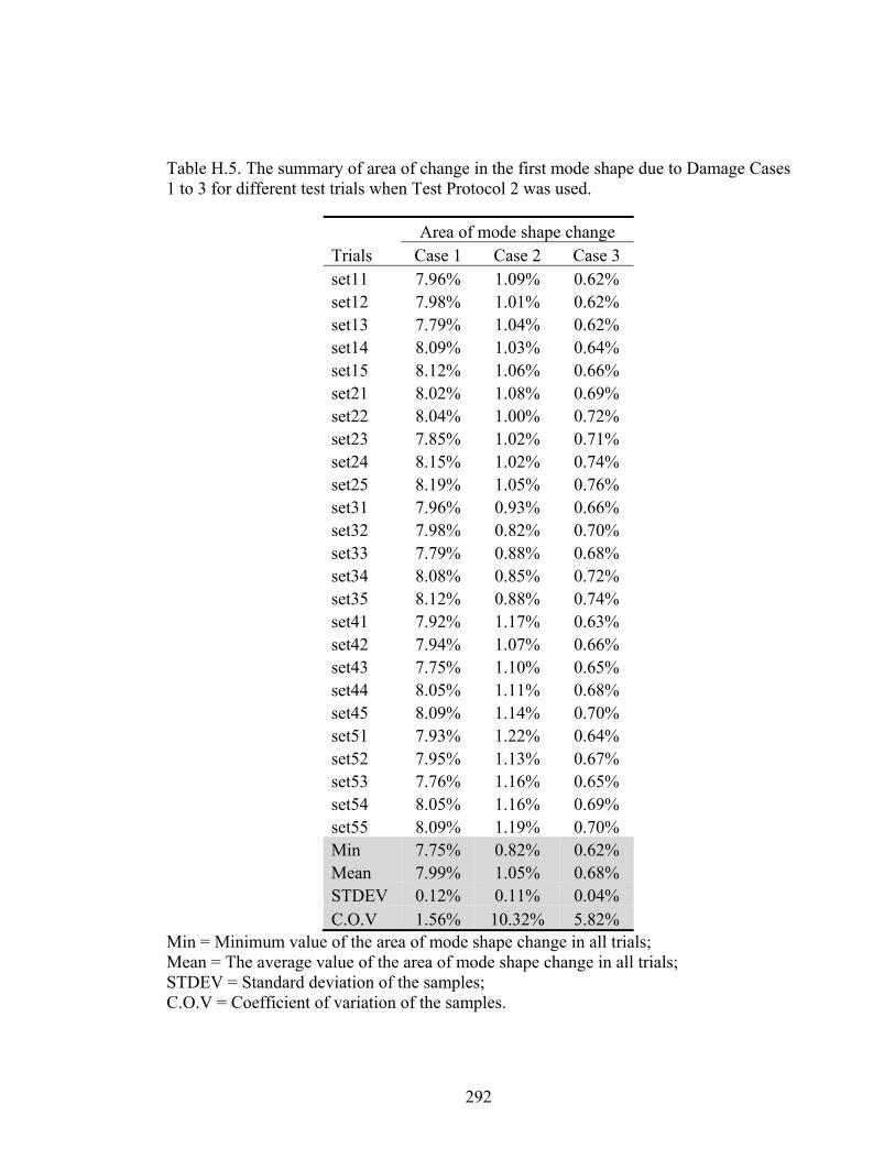
292
Table H.5. The summary of area of change in the first mode shape due to Damage Cases 1 to 3 for different test trials when Test Protocol 2 was used.
Area of mode shape change Trials Case 1 Case 2 Case 3 set11 7.96% 1.09% 0.62% set12 7.98% 1.01% 0.62% set13 7.79% 1.04% 0.62% set14 8.09% 1.03% 0.64% set15 8.12% 1.06% 0.66% set21 8.02% 1.08% 0.69% set22 8.04% 1.00% 0.72% set23 7.85% 1.02% 0.71% set24 8.15% 1.02% 0.74% set25 8.19% 1.05% 0.76% set31 7.96% 0.93% 0.66% set32 7.98% 0.82% 0.70% set33 7.79% 0.88% 0.68% set34 8.08% 0.85% 0.72% set35 8.12% 0.88% 0.74% set41 7.92% 1.17% 0.63% set42 7.94% 1.07% 0.66% set43 7.75% 1.10% 0.65% set44 8.05% 1.11% 0.68% set45 8.09% 1.14% 0.70% set51 7.93% 1.22% 0.64% set52 7.95% 1.13% 0.67% set53 7.76% 1.16% 0.65% set54 8.05% 1.16% 0.69% set55 8.09% 1.19% 0.70% Min 7.75% 0.82% 0.62% Mean 7.99% 1.05% 0.68% STDEV 0.12% 0.11% 0.04% C.O.V 1.56% 10.32% 5.82%
Min = Minimum value of the area of mode shape change in all trials; Mean = The average value of the area of mode shape change in all trials; STDEV = Standard deviation of the samples; C.O.V = Coefficient of variation of the samples.

293
Table H.6. The summary of area of change in the first mode shape due to Damage Cases 4 to 9 for different test trials when Test Protocol 2 was used.
Area of mode shape change Trials Case 4 Case 5 Case 6 Case 7 Case 8 Case 9 set11 1.69% 1.43% 2.18% 0.88% 2.19% 2.01% set12 1.73% 1.40% 2.15% 0.81% 2.14% 1.99% set13 1.75% 1.79% 2.19% 0.82% 2.11% 2.00% set14 1.74% 1.36% 2.17% 0.86% 1.94% 1.98% set15 1.68% 1.37% 2.14% 0.76% 1.99% 1.95% set21 1.71% 1.43% 2.17% 0.87% 2.21% 2.01% set22 1.75% 1.41% 2.14% 0.80% 2.15% 1.98% set23 1.77% 1.80% 2.19% 0.80% 2.10% 2.00% set24 1.75% 1.36% 2.16% 0.85% 1.95% 1.98% set25 1.70% 1.37% 2.13% 0.75% 1.99% 1.94% set31 1.72% 1.27% 1.99% 0.73% 2.04% 1.82% set32 1.76% 1.24% 1.95% 0.65% 1.98% 1.79% set33 1.78% 1.63% 2.01% 0.66% 1.94% 1.81% set34 1.76% 1.19% 1.98% 0.71% 1.77% 1.79% set35 1.71% 1.20% 1.95% 0.62% 1.81% 1.74% set41 1.77% 1.58% 2.29% 0.94% 2.33% 2.12% set42 1.82% 1.55% 2.24% 0.89% 2.27% 2.10% set43 1.84% 1.94% 2.29% 0.88% 2.24% 2.11% set44 1.83% 1.50% 2.27% 0.92% 2.08% 2.09% set45 1.76% 1.51% 2.24% 0.82% 2.11% 2.05% set51 1.73% 1.58% 2.29% 1.00% 2.36% 2.15% set52 1.77% 1.56% 2.24% 0.93% 2.29% 2.13% set53 1.80% 1.95% 2.32% 0.93% 2.25% 2.14% set54 1.78% 1.51% 2.27% 0.97% 2.10% 2.12% set55 1.72% 1.52% 2.24% 0.88% 2.14% 2.08% Min 1.68% 1.19% 1.95% 0.62% 1.77% 1.74% Mean 1.75% 1.50% 2.17% 0.83% 2.10% 1.99% STDEV 0.04% 0.21% 0.11% 0.10% 0.15% 0.12% C.O.V 2.40% 13.74% 5.18% 12.09% 7.34% 6.11%
Min = Minimum value of the area of mode shape change in all trials; Mean = The average value of the area of mode shape change in all trials; STDEV = Standard deviation of the samples; C.O.V = Coefficient of variation of the samples.

294
Table H.7. The summary of area of change in the first mode shape due to Damage Cases 10 to 15 for different test trials when Test Protocol 2 was used.
Area of mode shape change Trials Case 10 Case 11 Case 12 Case 13 Case 14 Case 15 set11 2.39% 0.23% 0.86% 0.81% 0.22% 0.51% set12 2.28% 0.23% 0.89% 0.83% 0.23% 0.56% set13 2.40% 0.20% 0.75% 0.70% 0.34% 0.58% set14 2.35% 0.22% 0.75% 0.61% 0.41% 0.57% set15 2.25% 0.20% 0.73% 0.70% 0.32% 0.50% set21 2.34% 0.30% 0.92% 0.80% 0.20% 0.50% set22 2.24% 0.32% 0.95% 0.83% 0.17% 0.54% set23 2.36% 0.29% 0.81% 0.69% 0.28% 0.57% set24 2.31% 0.29% 0.78% 0.60% 0.35% 0.57% set25 2.21% 0.30% 0.79% 0.70% 0.31% 0.51% set31 2.38% 0.22% 0.88% 0.93% 0.25% 0.34% set32 2.28% 0.22% 0.91% 0.95% 0.24% 0.40% set33 2.39% 0.20% 0.76% 0.80% 0.17% 0.41% set34 2.35% 0.20% 0.77% 0.69% 0.19% 0.42% set35 2.25% 0.20% 0.74% 0.81% 0.19% 0.36% set41 2.36% 0.32% 0.83% 1.00% 0.34% 0.35% set42 2.25% 0.31% 0.87% 1.03% 0.32% 0.38% set43 2.37% 0.29% 0.71% 0.88% 0.16% 0.39% set44 2.32% 0.31% 0.68% 0.77% 0.15% 0.40% set45 2.22% 0.28% 0.70% 0.89% 0.22% 0.33% set51 2.30% 0.32% 0.84% 0.93% 0.23% 0.41% set52 2.20% 0.32% 0.87% 0.95% 0.21% 0.46% set53 2.32% 0.27% 0.72% 0.80% 0.16% 0.47% set54 2.27% 0.30% 0.72% 0.69% 0.23% 0.48% set55 2.17% 0.30% 0.71% 0.81% 0.19% 0.42% Min 2.17% 0.20% 0.68% 0.60% 0.15% 0.33% Mean 2.30% 0.26% 0.80% 0.81% 0.24% 0.46% STDEV 0.07% 0.05% 0.08% 0.12% 0.07% 0.08% C.O.V 2.85% 17.81% 9.93% 14.54% 29.24% 17.47%
Min = Minimum value of the area of mode shape change in all trials; Mean = The average value of the area of mode shape change in all trials; STDEV = Standard deviation of the samples; C.O.V = Coefficient of variation of the samples.

295
Table H.8. The summary of area of change in the first mode shape due to Damage Cases 16 to 21 for different test trials when Test Protocol 2 was used.
Area of mode shape change Trials Case 16 Case 17 Case 18 Case 19 Case 20 Case 21 set11 0.21% 7.12% 6.53% 6.54% 5.98% 7.88% set12 0.19% 7.22% 6.50% 6.67% 6.02% 7.83% set13 0.22% 7.19% 6.52% 6.64% 6.02% 7.90% set14 0.18% 7.16% 6.48% 6.48% 6.02% 7.95% set15 0.17% 7.17% 6.46% 6.61% 6.09% 7.80% set21 0.25% 7.18% 6.60% 6.61% 6.05% 7.94% set22 0.24% 7.28% 6.57% 6.73% 6.08% 7.89% set23 0.21% 7.26% 6.59% 6.72% 6.08% 7.96% set24 0.17% 7.22% 6.55% 6.55% 6.09% 8.01% set25 0.16% 7.23% 6.53% 6.69% 6.15% 7.86% set31 0.20% 7.12% 6.53% 6.54% 5.98% 7.88% set32 0.18% 7.22% 6.50% 6.66% 6.02% 7.83% set33 0.22% 7.19% 6.52% 6.64% 6.01% 7.89% set34 0.18% 7.16% 6.48% 6.48% 6.02% 7.95% set35 0.20% 7.17% 6.46% 6.61% 6.08% 7.80% set41 0.23% 7.08% 6.49% 6.50% 5.95% 7.84% set42 0.22% 7.18% 6.47% 6.63% 5.98% 7.79% set43 0.25% 7.16% 6.48% 6.61% 5.98% 7.86% set44 0.20% 7.12% 6.45% 6.45% 5.99% 7.91% set45 0.21% 7.13% 6.43% 6.58% 6.05% 7.76% set51 0.28% 7.09% 6.50% 6.51% 5.95% 7.85% set52 0.24% 7.19% 6.47% 6.63% 5.99% 7.80% set53 0.21% 7.16% 6.49% 6.61% 5.99% 7.86% set54 0.20% 7.13% 6.45% 6.45% 5.99% 7.92% set55 0.19% 7.14% 6.43% 6.58% 6.05% 7.77% Min 0.16% 7.08% 6.43% 6.45% 5.95% 7.76% Mean 0.21% 7.17% 6.50% 6.59% 6.02% 7.87% STDEV 0.03% 0.05% 0.04% 0.08% 0.05% 0.06% C.O.V 14.01% 0.70% 0.68% 1.21% 0.83% 0.82%
Min = Minimum value of the area of mode shape change in all trials; Mean = The average value of the area of mode shape change in all trials; STDEV = Standard deviation of the samples; C.O.V = Coefficient of variation of the samples.

296
Table H.9. The summary of area of change in the first mode shape due to Damage Cases 22 to 26 for different test trials when Test Protocol 2 was used.
Area of mode shape change Trials Case 22 Case 23 Case 24 Case 25 Case 26 set11 7.77% 1.47% 1.40% 1.29% 1.17% set12 7.78% 1.45% 1.37% 1.30% 1.19% set13 7.78% 1.33% 1.25% 1.24% 1.17% set14 7.81% 1.23% 1.21% 1.33% 1.19% set15 7.81% 1.34% 1.23% 1.30% 1.27% set21 7.84% 1.54% 1.47% 1.37% 1.24% set22 7.84% 1.52% 1.44% 1.37% 1.26% set23 7.84% 1.40% 1.32% 1.32% 1.24% set24 7.87% 1.30% 1.28% 1.40% 1.26% set25 7.88% 1.41% 1.30% 1.37% 1.34% set31 7.77% 1.50% 1.43% 1.34% 1.21% set32 7.78% 1.48% 1.39% 1.35% 1.23% set33 7.78% 1.36% 1.28% 1.30% 1.22% set34 7.80% 1.26% 1.23% 1.37% 1.23% set35 7.81% 1.38% 1.25% 1.35% 1.31% set41 7.74% 1.44% 1.38% 1.27% 1.14% set42 7.74% 1.42% 1.34% 1.28% 1.17% set43 7.74% 1.31% 1.23% 1.22% 1.16% set44 7.77% 1.20% 1.19% 1.30% 1.16% set45 7.78% 1.32% 1.21% 1.28% 1.24% set51 7.74% 1.44% 1.37% 1.27% 1.15% set52 7.75% 1.42% 1.33% 1.28% 1.16% set53 7.75% 1.30% 1.22% 1.23% 1.15% set54 7.78% 1.20% 1.18% 1.31% 1.16% set55 7.78% 1.31% 1.20% 1.28% 1.24% Min 7.74% 1.20% 1.18% 1.22% 1.14% Mean 7.79% 1.37% 1.30% 1.31% 1.21% STDEV 0.04% 0.10% 0.09% 0.05% 0.05% C.O.V 0.52% 7.03% 6.83% 3.65% 4.35%
Min = Minimum value of the area of mode shape change in all trials; Mean = The average value of the area of mode shape change in all trials; STDEV = Standard deviation of the samples; C.O.V = Coefficient of variation of the samples.
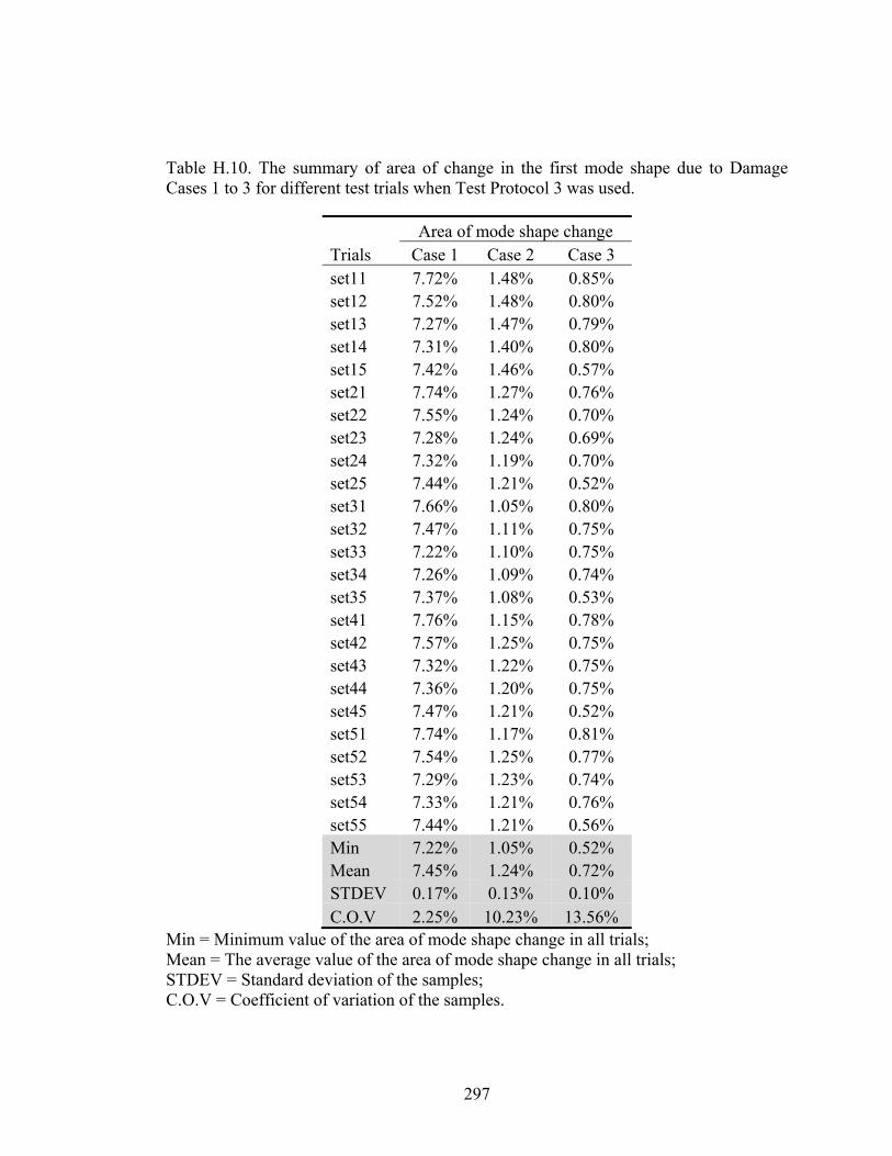
297
Table H.10. The summary of area of change in the first mode shape due to Damage Cases 1 to 3 for different test trials when Test Protocol 3 was used.
Area of mode shape change Trials Case 1 Case 2 Case 3 set11 7.72% 1.48% 0.85% set12 7.52% 1.48% 0.80% set13 7.27% 1.47% 0.79% set14 7.31% 1.40% 0.80% set15 7.42% 1.46% 0.57% set21 7.74% 1.27% 0.76% set22 7.55% 1.24% 0.70% set23 7.28% 1.24% 0.69% set24 7.32% 1.19% 0.70% set25 7.44% 1.21% 0.52% set31 7.66% 1.05% 0.80% set32 7.47% 1.11% 0.75% set33 7.22% 1.10% 0.75% set34 7.26% 1.09% 0.74% set35 7.37% 1.08% 0.53% set41 7.76% 1.15% 0.78% set42 7.57% 1.25% 0.75% set43 7.32% 1.22% 0.75% set44 7.36% 1.20% 0.75% set45 7.47% 1.21% 0.52% set51 7.74% 1.17% 0.81% set52 7.54% 1.25% 0.77% set53 7.29% 1.23% 0.74% set54 7.33% 1.21% 0.76% set55 7.44% 1.21% 0.56% Min 7.22% 1.05% 0.52% Mean 7.45% 1.24% 0.72% STDEV 0.17% 0.13% 0.10% C.O.V 2.25% 10.23% 13.56%
Min = Minimum value of the area of mode shape change in all trials; Mean = The average value of the area of mode shape change in all trials; STDEV = Standard deviation of the samples; C.O.V = Coefficient of variation of the samples.

298
Table H.11. The summary of area of change in the first mode shape due to Damage Cases 4 to 9 for different test trials when Test Protocol 3 was used.
Area of mode shape change Trials Case 4 Case 5 Case 6 Case 7 Case 8 Case 9 set11 0.94% 1.58% 2.43% 1.08% 2.28% 2.28% set12 0.95% 1.36% 2.56% 1.18% 2.27% 2.32% set13 0.83% 1.64% 2.53% 1.08% 2.24% 2.28% set14 1.00% 1.36% 2.58% 1.06% 2.25% 2.35% set15 0.83% 1.31% 2.46% 1.02% 2.22% 2.33% set21 0.99% 1.32% 2.23% 0.80% 2.11% 2.13% set22 1.00% 1.15% 2.34% 0.92% 2.11% 2.17% set23 0.89% 1.39% 2.30% 0.82% 2.06% 2.12% set24 1.05% 1.09% 2.36% 0.81% 2.10% 2.20% set25 0.89% 1.07% 2.28% 0.75% 2.06% 2.17% set31 1.02% 1.03% 2.12% 0.63% 1.97% 1.90% set32 1.02% 1.11% 2.21% 0.71% 1.92% 1.91% set33 0.90% 1.46% 2.21% 0.69% 1.88% 1.94% set34 1.07% 1.15% 2.19% 0.72% 1.94% 1.89% set35 0.90% 1.00% 2.13% 0.70% 1.91% 1.93% set41 0.92% 1.10% 2.15% 0.81% 2.05% 1.97% set42 0.93% 1.19% 2.27% 0.91% 2.00% 1.98% set43 0.86% 1.52% 2.25% 0.86% 1.95% 2.01% set44 1.01% 1.24% 2.23% 0.89% 2.00% 1.96% set45 0.86% 1.07% 2.17% 0.87% 1.96% 1.98% set51 1.16% 1.24% 2.22% 0.80% 2.11% 2.04% set52 1.17% 1.23% 2.33% 0.92% 2.07% 2.06% set53 1.07% 1.55% 2.32% 0.85% 2.02% 2.08% set54 1.24% 1.27% 2.30% 0.87% 2.06% 2.09% set55 1.07% 1.11% 2.25% 0.87% 2.03% 2.07% Min 0.83% 1.00% 2.12% 0.63% 1.88% 1.89% Mean 0.98% 1.26% 2.30% 0.87% 2.06% 2.09% STDEV 0.11% 0.18% 0.13% 0.14% 0.12% 0.14% C.O.V 11.12% 14.50% 5.63% 15.85% 5.63% 6.92%
Min = Minimum value of the area of mode shape change in all trials; Mean = The average value of the area of mode shape change in all trials; STDEV = Standard deviation of the samples; C.O.V = Coefficient of variation of the samples.

299
Table H.12. The summary of area of change in the first mode shape due to Damage Cases 10 to 15 for different test trials when Test Protocol 3 was used.
Area of mode shape change Trials Case 10 Case 11 Case 12 Case 13 Case 14 Case 15 set11 0.77% 0.33% 1.20% 1.08% 0.30% 0.92% set12 0.88% 0.34% 1.11% 1.05% 0.38% 1.01% set13 0.93% 0.28% 1.12% 1.11% 0.34% 1.02% set14 0.90% 0.29% 1.09% 1.04% 0.40% 1.01% set15 0.85% 0.26% 1.16% 1.09% 0.35% 1.10% set21 0.80% 0.35% 1.19% 1.16% 0.30% 0.88% set22 0.91% 0.39% 1.13% 1.13% 0.29% 0.96% set23 0.97% 0.34% 1.15% 1.18% 0.30% 0.98% set24 0.93% 0.30% 1.09% 1.11% 0.27% 0.97% set25 0.88% 0.29% 1.17% 1.16% 0.27% 1.05% set31 0.76% 0.31% 1.26% 1.14% 0.32% 0.88% set32 0.87% 0.29% 1.17% 1.11% 0.37% 0.97% set33 0.93% 0.30% 1.20% 1.16% 0.30% 0.99% set34 0.89% 0.28% 1.16% 1.10% 0.34% 0.98% set35 0.85% 0.28% 1.23% 1.12% 0.30% 1.05% set41 0.83% 0.31% 1.19% 1.21% 0.35% 0.80% set42 0.95% 0.29% 1.11% 1.16% 0.37% 0.90% set43 1.00% 0.25% 1.13% 1.22% 0.33% 0.90% set44 0.96% 0.25% 1.11% 1.15% 0.33% 0.89% set45 0.91% 0.27% 1.16% 1.17% 0.35% 0.99% set51 0.81% 0.35% 1.17% 1.08% 0.22% 0.94% set52 0.93% 0.37% 1.09% 1.05% 0.34% 1.01% set53 0.97% 0.29% 1.11% 1.11% 0.29% 1.04% set54 0.94% 0.29% 1.08% 1.04% 0.29% 1.02% set55 0.89% 0.30% 1.14% 1.07% 0.26% 1.10% Min 0.76% 0.25% 1.08% 1.04% 0.22% 0.80% Mean 0.89% 0.30% 1.15% 1.12% 0.32% 0.98% STDEV 0.06% 0.04% 0.05% 0.05% 0.04% 0.07% C.O.V 7.11% 11.81% 3.99% 4.66% 13.25% 7.47%
Min = Minimum value of the area of mode shape change in all trials; Mean = The average value of the area of mode shape change in all trials; STDEV = Standard deviation of the samples; C.O.V = Coefficient of variation of the samples.

300
Table H.13. The summary of area of change in the first mode shape due to Damage Cases 16 to 21 for different test trials when Test Protocol 3 was used.
Area of mode shape change Trials Case 16 Case 17 Case 18 Case 19 Case 20 Case 21 set11 0.38% 6.51% 5.79% 4.99% 5.46% 6.19% set12 0.45% 6.52% 5.86% 4.97% 5.42% 6.32% set13 0.51% 6.53% 5.87% 5.01% 5.46% 6.34% set14 0.43% 6.56% 5.83% 4.86% 5.41% 6.30% set15 0.41% 6.57% 6.05% 5.06% 5.39% 6.28% set21 0.30% 6.53% 5.82% 5.01% 5.48% 6.22% set22 0.38% 6.55% 5.88% 4.99% 5.44% 6.34% set23 0.46% 6.55% 5.90% 5.03% 5.48% 6.36% set24 0.36% 6.59% 5.86% 4.88% 5.43% 6.33% set25 0.38% 6.59% 6.07% 5.08% 5.41% 6.30% set31 0.23% 6.46% 5.73% 4.94% 5.40% 6.14% set32 0.35% 6.46% 5.80% 4.92% 5.37% 6.26% set33 0.37% 6.47% 5.82% 4.96% 5.40% 6.28% set34 0.25% 6.51% 5.77% 4.80% 5.36% 6.25% set35 0.34% 6.51% 5.99% 5.01% 5.34% 6.22% set41 0.30% 6.56% 5.83% 5.04% 5.50% 6.23% set42 0.44% 6.56% 5.90% 5.02% 5.47% 6.36% set43 0.35% 6.57% 5.91% 5.06% 5.50% 6.38% set44 0.37% 6.60% 5.87% 4.90% 5.46% 6.35% set45 0.36% 6.61% 6.09% 5.11% 5.43% 6.32% set51 0.24% 6.53% 5.81% 5.01% 5.48% 6.21% set52 0.34% 6.54% 5.88% 4.99% 5.44% 6.34% set53 0.36% 6.55% 5.89% 5.03% 5.48% 6.36% set54 0.26% 6.58% 5.85% 4.88% 5.43% 6.32% set55 0.33% 6.59% 6.07% 5.08% 5.41% 6.29% Min 0.23% 6.46% 5.73% 4.80% 5.34% 6.14% Mean 0.36% 6.54% 5.89% 4.99% 5.43% 6.29% STDEV 0.07% 0.04% 0.10% 0.08% 0.04% 0.06% C.O.V 19.46% 0.63% 1.64% 1.53% 0.79% 0.99%
Min = Minimum value of the area of mode shape change in all trials; Mean = The average value of the area of mode shape change in all trials; STDEV = Standard deviation of the samples; C.O.V = Coefficient of variation of the samples.

301
Table H.14. The summary of area of change in the first mode shape due to Damage Cases 22 to 26 for different test trials when Test Protocol 3 was used.
Area of mode shape change Trials Case 22 Case 23 Case 24 Case 25 Case 26 set11 6.07% 2.00% 2.12% 1.41% 1.38% set12 6.13% 2.03% 2.08% 1.39% 1.47% set13 6.13% 2.10% 2.08% 1.40% 1.39% set14 6.12% 2.02% 2.03% 1.35% 1.42% set15 6.18% 2.08% 2.13% 1.32% 1.39% set21 6.09% 2.07% 2.15% 1.48% 1.38% set22 6.16% 2.10% 2.10% 1.44% 1.45% set23 6.15% 2.17% 2.09% 1.45% 1.37% set24 6.15% 2.09% 2.07% 1.40% 1.41% set25 6.20% 2.13% 2.14% 1.36% 1.38% set31 6.01% 2.12% 2.22% 1.50% 1.43% set32 6.08% 2.15% 2.17% 1.46% 1.49% set33 6.07% 2.22% 2.17% 1.48% 1.42% set34 6.07% 2.14% 2.13% 1.43% 1.47% set35 6.12% 2.19% 2.22% 1.39% 1.43% set41 6.11% 2.00% 2.11% 1.36% 1.32% set42 6.18% 2.02% 2.06% 1.33% 1.43% set43 6.17% 2.08% 2.07% 1.32% 1.33% set44 6.16% 2.02% 2.01% 1.27% 1.36% set45 6.22% 2.06% 2.11% 1.25% 1.33% set51 6.09% 2.00% 2.12% 1.41% 1.37% set52 6.15% 2.03% 2.07% 1.39% 1.46% set53 6.15% 2.11% 2.08% 1.40% 1.38% set54 6.14% 2.02% 2.02% 1.35% 1.41% set55 6.20% 2.08% 2.12% 1.31% 1.38% Min 6.01% 2.00% 2.01% 1.25% 1.32% Mean 6.13% 2.08% 2.11% 1.39% 1.40% STDEV 0.05% 0.06% 0.05% 0.06% 0.04% C.O.V 0.81% 3.02% 2.59% 4.63% 3.17%
Min = Minimum value of the area of mode shape change in all trials; Mean = The average value of the area of mode shape change in all trials; STDEV = Standard deviation of the samples; C.O.V = Coefficient of variation of the samples.

302
Table H.15. The summary of area of change in the first mode shape due to Damage Cases 1 to 3 for different test trials when Test Protocol 4 was used.
Area of mode shape change Trials Case 1 Case 2 Case 3 set11 7.23% 1.49% 0.70% set12 9.10% 1.33% 0.75% set13 7.72% 1.29% 0.84% set14 7.13% 1.37% 0.70% set15 8.28% 1.40% 0.85% set21 7.13% 3.58% 0.73% set22 9.02% 3.48% 0.76% set23 7.63% 3.46% 0.82% set24 7.03% 3.55% 0.74% set25 8.20% 3.49% 0.82% set31 7.18% 2.33% 0.74% set32 9.21% 2.22% 0.81% set33 7.82% 2.18% 0.89% set34 7.08% 2.23% 0.78% set35 8.39% 2.26% 0.86% set41 7.32% 1.38% 0.69% set42 9.34% 1.29% 0.73% set43 7.95% 1.21% 0.75% set44 7.22% 1.34% 0.66% set45 8.53% 1.31% 0.77% set51 7.19% 2.75% 0.81% set52 9.13% 2.65% 0.86% set53 7.78% 2.61% 0.96% set54 7.07% 2.69% 0.85% set55 8.33% 2.71% 0.90% Min 7.03% 1.21% 0.66% Mean 7.92% 2.22% 0.79% STDEV 0.79% 0.85% 0.07% C.O.V 9.91% 38.05% 9.28%
Min = Minimum value of the area of mode shape change in all trials; Mean = The average value of the area of mode shape change in all trials; STDEV = Standard deviation of the samples; C.O.V = Coefficient of variation of the samples.
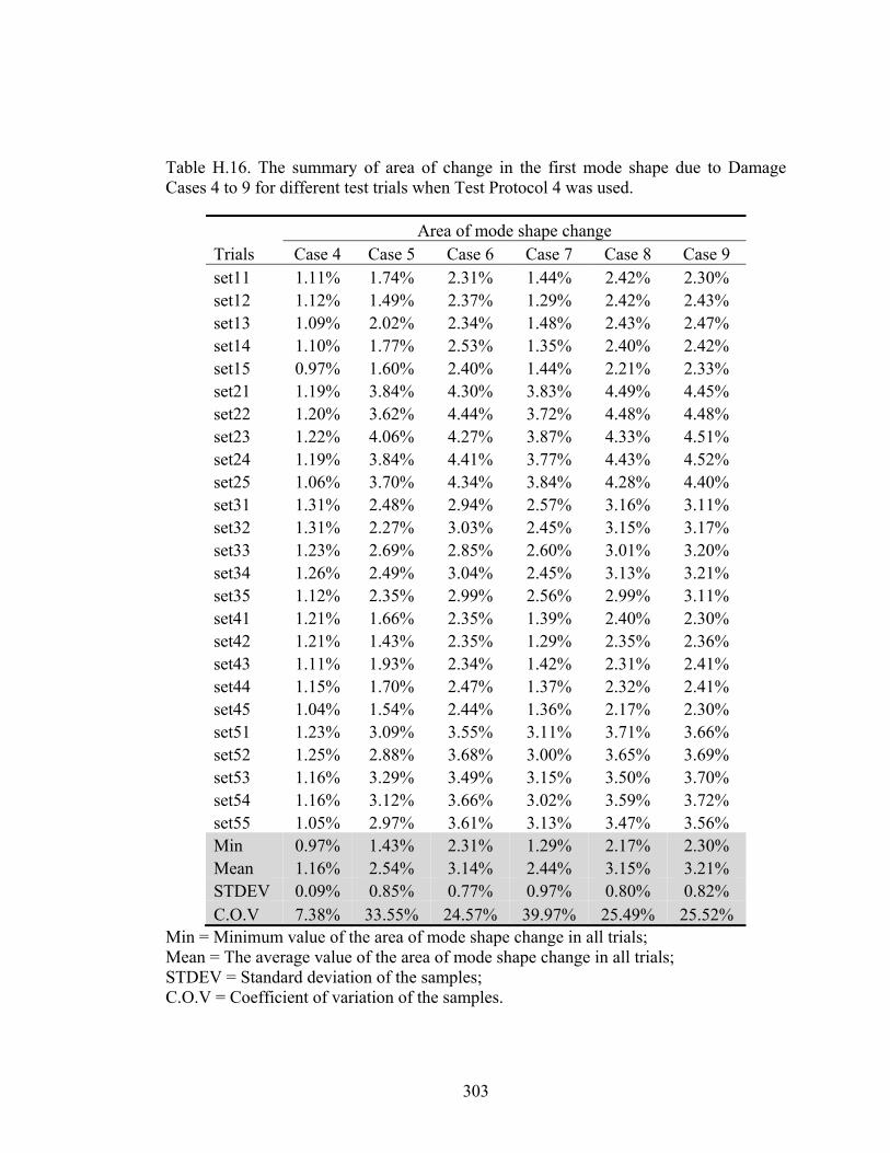
303
Table H.16. The summary of area of change in the first mode shape due to Damage Cases 4 to 9 for different test trials when Test Protocol 4 was used.
Area of mode shape change Trials Case 4 Case 5 Case 6 Case 7 Case 8 Case 9 set11 1.11% 1.74% 2.31% 1.44% 2.42% 2.30% set12 1.12% 1.49% 2.37% 1.29% 2.42% 2.43% set13 1.09% 2.02% 2.34% 1.48% 2.43% 2.47% set14 1.10% 1.77% 2.53% 1.35% 2.40% 2.42% set15 0.97% 1.60% 2.40% 1.44% 2.21% 2.33% set21 1.19% 3.84% 4.30% 3.83% 4.49% 4.45% set22 1.20% 3.62% 4.44% 3.72% 4.48% 4.48% set23 1.22% 4.06% 4.27% 3.87% 4.33% 4.51% set24 1.19% 3.84% 4.41% 3.77% 4.43% 4.52% set25 1.06% 3.70% 4.34% 3.84% 4.28% 4.40% set31 1.31% 2.48% 2.94% 2.57% 3.16% 3.11% set32 1.31% 2.27% 3.03% 2.45% 3.15% 3.17% set33 1.23% 2.69% 2.85% 2.60% 3.01% 3.20% set34 1.26% 2.49% 3.04% 2.45% 3.13% 3.21% set35 1.12% 2.35% 2.99% 2.56% 2.99% 3.11% set41 1.21% 1.66% 2.35% 1.39% 2.40% 2.30% set42 1.21% 1.43% 2.35% 1.29% 2.35% 2.36% set43 1.11% 1.93% 2.34% 1.42% 2.31% 2.41% set44 1.15% 1.70% 2.47% 1.37% 2.32% 2.41% set45 1.04% 1.54% 2.44% 1.36% 2.17% 2.30% set51 1.23% 3.09% 3.55% 3.11% 3.71% 3.66% set52 1.25% 2.88% 3.68% 3.00% 3.65% 3.69% set53 1.16% 3.29% 3.49% 3.15% 3.50% 3.70% set54 1.16% 3.12% 3.66% 3.02% 3.59% 3.72% set55 1.05% 2.97% 3.61% 3.13% 3.47% 3.56% Min 0.97% 1.43% 2.31% 1.29% 2.17% 2.30% Mean 1.16% 2.54% 3.14% 2.44% 3.15% 3.21% STDEV 0.09% 0.85% 0.77% 0.97% 0.80% 0.82% C.O.V 7.38% 33.55% 24.57% 39.97% 25.49% 25.52%
Min = Minimum value of the area of mode shape change in all trials; Mean = The average value of the area of mode shape change in all trials; STDEV = Standard deviation of the samples; C.O.V = Coefficient of variation of the samples.

304
Table H.17. The summary of area of change in the first mode shape due to Damage Cases 10 to 15 for different test trials when Test Protocol 4 was used.
Area of mode shape change Trials Case 10 Case 11 Case 12 Case 13 Case 14 Case 15 set11 1.08% 0.56% 3.21% 1.98% 0.98% 1.19% set12 0.97% 0.55% 2.36% 1.85% 0.81% 1.29% set13 1.03% 0.52% 2.47% 1.96% 0.67% 1.01% set14 0.90% 0.45% 2.41% 2.21% 1.01% 1.23% set15 1.13% 0.64% 2.36% 1.97% 2.02% 1.39% set21 1.08% 0.44% 3.12% 1.39% 1.09% 1.01% set22 1.02% 0.55% 2.29% 1.44% 0.88% 1.05% set23 1.02% 0.55% 2.34% 1.41% 0.75% 0.86% set24 0.94% 0.43% 2.33% 1.41% 1.06% 0.96% set25 1.16% 0.51% 2.30% 1.25% 2.14% 1.18% set31 1.18% 0.41% 2.97% 1.80% 1.00% 0.91% set32 1.06% 0.54% 2.29% 1.88% 0.84% 0.91% set33 1.08% 0.51% 2.43% 1.85% 0.64% 0.74% set34 1.00% 0.43% 2.37% 1.81% 0.98% 0.88% set35 1.23% 0.61% 2.31% 1.67% 2.02% 1.07% set41 1.07% 0.48% 2.94% 1.72% 0.90% 1.21% set42 0.89% 0.64% 2.22% 1.82% 0.84% 1.27% set43 0.95% 0.58% 2.44% 1.76% 0.71% 0.98% set44 0.84% 0.53% 2.35% 1.70% 0.94% 1.22% set45 1.05% 0.54% 2.23% 1.58% 1.89% 1.36% set51 1.08% 0.54% 2.98% 1.53% 0.79% 2.25% set52 0.94% 0.60% 2.30% 1.58% 0.63% 2.33% set53 0.98% 0.57% 2.46% 1.55% 0.51% 2.02% set54 0.87% 0.45% 2.40% 1.56% 0.83% 2.27% set55 1.09% 0.62% 2.30% 1.40% 1.89% 2.41% Min 0.84% 0.41% 2.22% 1.25% 0.51% 0.74% Mean 1.03% 0.53% 2.49% 1.68% 1.07% 1.32% STDEV 0.10% 0.07% 0.29% 0.23% 0.49% 0.51% C.O.V 9.61% 12.59% 11.83% 13.96% 45.65% 38.49%
Min = Minimum value of the area of mode shape change in all trials; Mean = The average value of the area of mode shape change in all trials; STDEV = Standard deviation of the samples; C.O.V = Coefficient of variation of the samples.

305
Table H.18. The summary of area of change in the first mode shape due to Damage Cases 16 to 21 for different test trials when Test Protocol 4 was used.
Area of mode shape change Trials Case 16 Case 17 Case 18 Case 19 Case 20 Case 21 set11 0.82% 6.23% 5.67% 4.70% 5.57% 5.85% set12 0.71% 6.33% 5.74% 4.76% 5.35% 5.86% set13 0.77% 6.33% 5.77% 4.63% 5.44% 5.69% set14 0.77% 6.25% 5.68% 4.66% 5.33% 5.84% set15 0.77% 6.32% 5.73% 4.76% 5.39% 5.91% set21 0.79% 6.13% 5.57% 4.60% 5.47% 5.75% set22 0.70% 6.23% 5.64% 4.67% 5.25% 5.77% set23 0.76% 6.23% 5.67% 4.57% 5.34% 5.59% set24 0.71% 6.15% 5.58% 4.56% 5.23% 5.74% set25 0.73% 6.22% 5.63% 4.67% 5.29% 5.81% set31 0.95% 6.20% 5.70% 4.69% 5.53% 5.80% set32 0.82% 6.30% 5.77% 4.72% 5.31% 5.82% set33 0.84% 6.28% 5.83% 4.67% 5.40% 5.66% set34 0.84% 6.22% 5.71% 4.68% 5.29% 5.80% set35 0.96% 6.28% 5.78% 4.81% 5.37% 5.86% set41 0.80% 6.34% 5.85% 4.83% 5.66% 5.94% set42 0.70% 6.44% 5.91% 4.86% 5.45% 5.96% set43 0.71% 6.43% 5.96% 4.79% 5.52% 5.80% set44 0.68% 6.35% 5.84% 4.82% 5.43% 5.94% set45 0.74% 6.43% 5.91% 4.95% 5.51% 6.00% set51 0.81% 6.15% 5.67% 4.64% 5.55% 5.77% set52 0.63% 6.26% 5.74% 4.70% 5.32% 5.79% set53 0.75% 6.27% 5.83% 4.65% 5.43% 5.62% set54 0.70% 6.21% 5.71% 4.65% 5.31% 5.77% set55 0.79% 6.25% 5.77% 4.78% 5.36% 5.83% Min 0.63% 6.13% 5.57% 4.56% 5.23% 5.59% Mean 0.77% 6.27% 5.75% 4.71% 5.40% 5.81% STDEV 0.08% 0.08% 0.10% 0.10% 0.11% 0.10% C.O.V 9.91% 1.33% 1.76% 2.03% 2.00% 1.75%
Min = Minimum value of the area of mode shape change in all trials; Mean = The average value of the area of mode shape change in all trials; STDEV = Standard deviation of the samples; C.O.V = Coefficient of variation of the samples.

306
Table H.19. The summary of area of change in the first mode shape due to Damage Cases 22 to 26 for different test trials when Test Protocol 4 was used.
Area of mode shape change Trials Case 22 Case 23 Case 24 Case 25 Case 26 set11 5.77% 2.39% 2.19% 2.92% 3.03% set12 5.60% 2.48% 2.31% 2.94% 2.84% set13 5.67% 2.37% 2.42% 2.67% 2.81% set14 5.63% 2.35% 2.11% 2.85% 2.84% set15 5.68% 2.33% 2.47% 2.96% 3.05% set21 5.67% 2.37% 2.11% 2.88% 2.98% set22 5.50% 2.44% 2.24% 2.91% 2.80% set23 5.57% 2.37% 2.38% 2.63% 2.76% set24 5.53% 2.34% 2.03% 2.81% 2.80% set25 5.58% 2.31% 2.36% 2.92% 3.01% set31 5.72% 2.43% 2.23% 2.95% 2.99% set32 5.55% 2.49% 2.32% 2.98% 2.84% set33 5.62% 2.43% 2.45% 2.71% 2.80% set34 5.59% 2.41% 2.11% 2.88% 2.85% set35 5.63% 2.38% 2.52% 2.99% 3.02% set41 5.87% 2.33% 2.21% 2.84% 2.86% set42 5.69% 2.42% 2.28% 2.87% 2.74% set43 5.76% 2.32% 2.38% 2.59% 2.69% set44 5.73% 2.27% 2.08% 2.78% 2.74% set45 5.77% 2.28% 2.57% 2.89% 2.91% set51 5.69% 2.44% 2.28% 3.01% 3.06% set52 5.52% 2.47% 2.38% 3.04% 2.83% set53 5.59% 2.43% 2.50% 2.76% 2.85% set54 5.56% 2.46% 2.17% 2.94% 2.87% set55 5.61% 2.41% 2.59% 3.02% 3.09% Min 5.50% 2.27% 2.03% 2.59% 2.69% Mean 5.64% 2.39% 2.31% 2.87% 2.88% STDEV 0.09% 0.06% 0.16% 0.12% 0.11% C.O.V 1.62% 2.57% 6.88% 4.26% 3.94%
Min = Minimum value of the area of mode shape change in all trials; Mean = The average value of the area of mode shape change in all trials; STDEV = Standard deviation of the samples; C.O.V = Coefficient of variation of the samples.

307
Table H.20. The summary of area of change in the first mode shape due to Damage Casess 1 to 3 for different test trials when Test Protocol 5 was used.
Area of mode shape changeTrials Case 1 Case 2 Case 3 set11 6.59% 1.82% 1.80% set12 6.43% 1.65% 2.32% set13 6.81% 0.96% 1.74% set14 6.35% 1.93% 1.68% set15 6.85% 1.45% 1.38% set21 6.64% 1.72% 1.92% set22 6.49% 1.67% 2.34% set23 6.86% 0.97% 1.79% set24 6.40% 1.81% 1.82% set25 6.91% 1.34% 1.44% set31 6.61% 1.82% 1.43% set32 6.46% 1.64% 1.84% set33 6.83% 0.96% 1.31% set34 6.37% 1.92% 1.34% set35 6.88% 1.44% 1.07% set41 6.50% 1.83% 1.73% set42 6.34% 1.75% 2.38% set43 6.71% 1.08% 1.77% set44 6.25% 1.96% 1.58% set45 6.76% 1.48% 1.39% set51 6.58% 1.45% 1.56% set52 6.43% 1.30% 2.04% set53 6.80% 0.62% 1.45% set54 6.34% 1.55% 1.45% set55 6.85% 1.07% 1.14% Min 6.25% 0.62% 1.07% Mean 6.60% 1.49% 1.67% STDEV 0.21% 0.37% 0.35% C.O.V 3.18% 24.72% 20.95%
Min = Minimum value of the area of mode shape change in all trials; Mean = The average value of the area of mode shape change in all trials; STDEV = Standard deviation of the samples; C.O.V = Coefficient of variation of the samples.

308
Table H.21. The summary of area of change in the first mode shape due to Damage Cases 4 to 9 for different test trials when Test Protocol 5 was used.
Area of mode shape change Trials Case 4 Case 5 Case 6 Case 7 Case 8 Case 9 set11 2.31% 1.16% 1.42% 0.60% 1.36% 1.31% set12 2.32% 1.43% 1.44% 0.55% 1.33% 1.38% set13 2.26% 1.21% 1.68% 0.50% 1.38% 1.11% set14 2.13% 1.11% 1.52% 0.99% 1.49% 1.52% set15 2.20% 1.34% 1.26% 0.85% 1.45% 1.23% set21 1.92% 1.04% 1.29% 0.62% 1.23% 1.18% set22 2.21% 1.37% 1.31% 0.45% 1.20% 1.24% set23 2.10% 1.13% 1.55% 0.66% 1.44% 0.98% set24 2.07% 1.03% 1.43% 0.95% 1.40% 1.44% set25 2.19% 1.22% 1.16% 0.77% 1.32% 1.06% set31 2.12% 1.38% 1.60% 0.89% 1.50% 1.39% set32 2.31% 1.65% 1.60% 0.59% 1.53% 1.54% set33 2.18% 1.43% 1.88% 0.52% 1.46% 1.24% set34 2.07% 1.21% 1.67% 1.20% 1.64% 1.75% set35 2.18% 1.53% 1.31% 0.77% 1.67% 1.30% set41 2.43% 0.92% 1.08% 0.54% 1.05% 0.89% set42 2.39% 1.22% 1.19% 0.56% 1.08% 0.96% set43 2.36% 0.99% 1.40% 0.60% 1.09% 0.76% set44 2.23% 0.84% 1.25% 0.73% 1.15% 1.19% set45 2.27% 1.06% 0.91% 0.53% 1.21% 0.86% set51 2.41% 1.42% 1.63% 0.86% 1.55% 1.43% set52 2.59% 1.69% 1.64% 0.47% 1.58% 1.57% set53 2.47% 1.48% 1.91% 0.68% 1.56% 1.28% set54 2.34% 1.26% 1.71% 1.24% 1.68% 1.80% set55 2.45% 1.57% 1.34% 0.76% 1.72% 1.34% Min 1.92% 0.84% 0.91% 0.45% 1.05% 0.76% Mean 2.26% 1.27% 1.45% 0.71% 1.40% 1.27% STDEV 0.15% 0.23% 0.24% 0.21% 0.20% 0.26% C.O.V 6.74% 17.88% 16.87% 29.96% 14.06% 20.70% Min = Minimum value of the area of mode shape change in all trials; Mean = The average value of the area of mode shape change in all trials; STDEV = Standard deviation of the samples; C.O.V = Coefficient of variation of the samples.

309
Table H.22. The summary of area of change in the first mode shape due to Damage Cases 10 to 15 for different test trials when Test Protocol 5 was used.
Area of mode shape change Trials Case 10 Case 11 Case 12 Case 13 Case 14 Case 15 set11 1.22% 0.90% 0.83% 0.90% 1.00% 0.68% set12 0.70% 1.38% 0.55% 0.57% 0.65% 0.70% set13 0.84% 1.36% 0.83% 0.37% 0.73% 0.60% set14 0.75% 0.91% 0.99% 0.98% 1.08% 0.56% set15 0.87% 1.67% 0.82% 0.56% 0.76% 0.72% set21 1.37% 0.55% 0.68% 0.90% 0.67% 0.49% set22 0.65% 1.06% 0.57% 0.59% 0.60% 0.74% set23 0.99% 0.79% 0.76% 0.65% 1.03% 0.52% set24 0.68% 0.47% 0.88% 1.04% 0.97% 0.54% set25 0.82% 1.29% 0.77% 0.83% 0.60% 0.63% set31 1.06% 0.44% 0.76% 0.72% 0.65% 0.68% set32 0.53% 0.93% 0.53% 0.61% 0.59% 0.85% set33 0.86% 0.84% 0.79% 0.49% 1.03% 0.72% set34 0.57% 0.60% 0.92% 0.86% 0.80% 0.97% set35 0.69% 1.13% 0.76% 0.61% 0.70% 0.67% set41 1.58% 0.64% 0.98% 0.73% 0.99% 0.65% set42 1.00% 1.18% 0.61% 0.58% 0.75% 0.91% set43 1.13% 0.90% 0.90% 0.44% 0.75% 0.77% set44 1.12% 0.44% 1.06% 0.78% 1.09% 0.60% set45 1.34% 1.38% 0.88% 0.49% 0.78% 0.79% set51 1.12% 0.82% 1.07% 0.68% 0.79% 0.61% set52 0.65% 1.38% 0.64% 0.51% 0.51% 0.70% set53 0.97% 1.15% 0.89% 0.62% 1.02% 0.49% set54 0.67% 0.63% 1.10% 0.77% 0.85% 0.58% set55 0.74% 1.64% 0.80% 0.68% 0.74% 0.70% Min 0.53% 0.44% 0.53% 0.37% 0.51% 0.49% Mean 0.92% 0.98% 0.81% 0.68% 0.81% 0.67% STDEV 0.27% 0.37% 0.16% 0.17% 0.17% 0.12% C.O.V 29.76% 37.55% 19.68% 25.39% 21.57% 18.04% Min = Minimum value of the area of mode shape change in all trials; Mean = The average value of the area of mode shape change in all trials; STDEV = Standard deviation of the samples; C.O.V = Coefficient of variation of the samples.
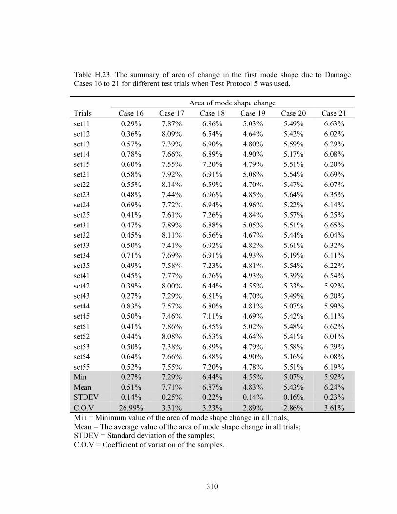
310
Table H.23. The summary of area of change in the first mode shape due to Damage Cases 16 to 21 for different test trials when Test Protocol 5 was used.
Area of mode shape change Trials Case 16 Case 17 Case 18 Case 19 Case 20 Case 21 set11 0.29% 7.87% 6.86% 5.03% 5.49% 6.63% set12 0.36% 8.09% 6.54% 4.64% 5.42% 6.02% set13 0.57% 7.39% 6.90% 4.80% 5.59% 6.29% set14 0.78% 7.66% 6.89% 4.90% 5.17% 6.08% set15 0.60% 7.55% 7.20% 4.79% 5.51% 6.20% set21 0.58% 7.92% 6.91% 5.08% 5.54% 6.69% set22 0.55% 8.14% 6.59% 4.70% 5.47% 6.07% set23 0.48% 7.44% 6.96% 4.85% 5.64% 6.35% set24 0.69% 7.72% 6.94% 4.96% 5.22% 6.14% set25 0.41% 7.61% 7.26% 4.84% 5.57% 6.25% set31 0.47% 7.89% 6.88% 5.05% 5.51% 6.65% set32 0.45% 8.11% 6.56% 4.67% 5.44% 6.04% set33 0.50% 7.41% 6.92% 4.82% 5.61% 6.32% set34 0.71% 7.69% 6.91% 4.93% 5.19% 6.11% set35 0.49% 7.58% 7.23% 4.81% 5.54% 6.22% set41 0.45% 7.77% 6.76% 4.93% 5.39% 6.54% set42 0.39% 8.00% 6.44% 4.55% 5.33% 5.92% set43 0.27% 7.29% 6.81% 4.70% 5.49% 6.20% set44 0.83% 7.57% 6.80% 4.81% 5.07% 5.99% set45 0.50% 7.46% 7.11% 4.69% 5.42% 6.11% set51 0.41% 7.86% 6.85% 5.02% 5.48% 6.62% set52 0.44% 8.08% 6.53% 4.64% 5.41% 6.01% set53 0.50% 7.38% 6.89% 4.79% 5.58% 6.29% set54 0.64% 7.66% 6.88% 4.90% 5.16% 6.08% set55 0.52% 7.55% 7.20% 4.78% 5.51% 6.19% Min 0.27% 7.29% 6.44% 4.55% 5.07% 5.92% Mean 0.51% 7.71% 6.87% 4.83% 5.43% 6.24% STDEV 0.14% 0.25% 0.22% 0.14% 0.16% 0.23% C.O.V 26.99% 3.31% 3.23% 2.89% 2.86% 3.61% Min = Minimum value of the area of mode shape change in all trials; Mean = The average value of the area of mode shape change in all trials; STDEV = Standard deviation of the samples; C.O.V = Coefficient of variation of the samples.

311
Table H.24. The summary of area of change in the first mode shape due to Damage Cases 22 to 26 for different test trials when Test Protocol 5 was used.
Area of mode shape change Trials Case 22 Case 23 Case 24 Case 25 Case 26 set11 5.87% 1.39% 1.20% 1.23% 1.36% set12 5.37% 1.03% 1.35% 0.81% 1.14% set13 5.47% 1.08% 1.60% 1.04% 0.89% set14 6.11% 1.52% 1.43% 1.07% 1.21% set15 5.19% 1.30% 1.26% 1.04% 0.78% set21 5.92% 1.36% 1.09% 1.16% 1.27% set22 5.42% 0.99% 1.25% 0.78% 1.04% set23 5.52% 0.97% 1.53% 0.99% 0.78% set24 6.17% 1.47% 1.32% 0.93% 1.14% set25 5.24% 1.18% 1.16% 0.98% 0.73% set31 5.89% 1.38% 1.08% 1.19% 1.31% set32 5.38% 0.98% 1.30% 0.79% 1.08% set33 5.49% 1.04% 1.57% 1.01% 0.82% set34 6.13% 1.49% 1.33% 1.01% 1.10% set35 5.21% 1.24% 1.20% 1.01% 0.70% set41 5.77% 1.48% 1.22% 1.32% 1.45% set42 5.27% 1.13% 1.46% 0.91% 1.24% set43 5.37% 1.21% 1.69% 1.13% 1.04% set44 6.02% 1.60% 1.47% 1.21% 1.11% set45 5.09% 1.41% 1.35% 1.14% 0.80% set51 5.86% 1.40% 1.19% 1.24% 1.39% set52 5.36% 1.12% 1.44% 0.87% 1.22% set53 5.46% 1.25% 1.63% 1.05% 1.10% set54 6.10% 1.53% 1.48% 1.28% 0.94% set55 5.18% 1.42% 1.33% 1.07% 0.80% Min 5.09% 0.97% 1.08% 0.78% 0.70% Mean 5.60% 1.28% 1.36% 1.05% 1.06% STDEV 0.35% 0.20% 0.17% 0.15% 0.22% C.O.V 6.25% 15.34% 12.32% 14.26% 21.09% Min = Minimum value of the area of mode shape change in all trials; Mean = The average value of the area of mode shape change in all trials; STDEV = Standard deviation of the samples; C.O.V = Coefficient of variation of the samples.

312
Table H.25. The summary of area of change in the first mode shape due to Damage Cases 1 to 3 for different test trials when Test Protocol 6 was used.
Area of mode shape change Trials Case 1 Case 2 Case 3 set11 7.13% 2.48% 3.74% set12 6.69% 2.60% 2.98% set13 8.21% 3.03% 2.78% set14 8.85% 2.55% 2.76% set15 7.25% 3.21% 3.74% set21 6.90% 2.22% 4.08% set22 6.69% 2.30% 3.12% set23 7.54% 3.10% 3.08% set24 8.34% 2.96% 3.39% set25 6.96% 3.81% 4.49% set31 5.32% 2.68% 1.80% set32 4.88% 2.98% 2.04% set33 6.56% 2.17% 2.04% set34 7.01% 2.29% 1.92% set35 5.56% 1.72% 2.69% set41 6.25% 3.55% 2.13% set42 5.88% 3.57% 1.75% set43 7.19% 3.07% 2.42% set44 7.95% 2.43% 2.45% set45 6.39% 3.53% 2.63% set51 6.28% 2.62% 2.35% set52 6.08% 2.97% 1.96% set53 6.81% 2.94% 2.02% set54 7.59% 2.59% 1.80% set55 6.27% 3.03% 2.07% Min 4.88% 1.72% 1.75% Mean 6.82% 2.82% 2.65% STDEV 0.95% 0.50% 0.77% C.O.V 13.85% 17.87% 28.92%
Min = Minimum value of the area of mode shape change in all trials; Mean = The average value of the area of mode shape change in all trials; STDEV = Standard deviation of the samples; C.O.V = Coefficient of variation of the samples.

313
Table H.26. The summary of area of change in the first mode shape due to Damage Cases 4 to 9 for different test trials when Test Protocol 6 was used.
Area of mode shape change Trials Case 4 Case 5 Case 6 Case 7 Case 8 Case 9 set11 3.87% 2.27% 2.56% 1.71% 2.66% 2.19% set12 4.28% 3.11% 2.21% 3.28% 3.68% 2.45% set13 4.03% 2.07% 2.49% 2.71% 3.37% 2.06% set14 3.11% 2.87% 3.02% 3.18% 2.92% 3.40% set15 3.71% 2.22% 2.85% 3.25% 2.40% 2.16% set21 3.57% 2.62% 1.67% 2.23% 3.17% 2.91% set22 3.72% 3.03% 2.81% 3.25% 3.21% 2.80% set23 3.61% 2.31% 1.78% 2.71% 3.03% 2.36% set24 2.99% 2.51% 2.20% 2.74% 2.64% 3.08% set25 3.58% 2.24% 2.17% 2.66% 2.10% 1.81% set31 3.64% 3.13% 3.00% 2.63% 3.75% 2.43% set32 3.52% 3.74% 2.40% 2.81% 3.09% 2.92% set33 3.55% 3.10% 2.19% 1.52% 2.55% 2.56% set34 3.43% 3.66% 3.34% 3.04% 2.96% 2.58% set35 3.58% 2.79% 2.83% 2.99% 2.21% 2.24% set41 4.42% 3.61% 3.14% 2.33% 2.27% 2.40% set42 3.93% 4.61% 2.32% 3.05% 3.98% 3.02% set43 4.24% 3.57% 3.02% 2.83% 2.82% 2.60% set44 3.52% 4.40% 3.66% 3.72% 3.40% 3.84% set45 3.55% 3.73% 3.20% 3.95% 3.16% 2.68% set51 3.78% 2.25% 2.63% 1.70% 2.67% 2.33% set52 4.16% 3.36% 2.21% 2.79% 3.37% 2.03% set53 4.34% 2.26% 2.35% 2.44% 2.83% 1.70% set54 3.51% 3.03% 2.81% 3.15% 2.76% 3.29% set55 3.92% 2.23% 2.62% 3.21% 2.42% 2.19% Min 2.99% 2.07% 1.67% 1.52% 2.10% 1.70% Mean 3.74% 2.99% 2.62% 2.80% 2.94% 2.56% STDEV 0.36% 0.71% 0.48% 0.58% 0.49% 0.51% C.O.V 9.57% 23.80% 18.39% 20.89% 16.71% 19.80%
Min = Minimum value of the area of mode shape change in all trials; Mean = The average value of the area of mode shape change in all trials; STDEV = Standard deviation of the samples; C.O.V = Coefficient of variation of the samples.

314
Table H.27. The summary of area of change in the first mode shape due to Damage Cases 10 to 15 for different test trials when Test Protocol 6 was used.
Area of mode shape change Trials Case 10 Case 11 Case 12 Case 13 Case 14 Case 15 set11 2.91% 2.53% 2.49% 2.30% 3.50% 3.31% set12 2.47% 2.95% 2.73% 2.50% 3.32% 2.93% set13 2.57% 2.61% 3.35% 3.41% 3.31% 4.12% set14 2.89% 2.31% 2.58% 2.58% 3.02% 3.32% set15 3.20% 2.85% 2.37% 2.55% 2.74% 2.95% set21 3.57% 3.17% 2.31% 3.05% 2.96% 2.70% set22 2.74% 1.97% 2.48% 2.67% 2.39% 3.48% set23 3.99% 2.79% 2.89% 3.82% 2.99% 3.56% set24 3.73% 4.19% 2.40% 3.52% 2.43% 3.64% set25 3.70% 2.40% 1.96% 3.11% 2.42% 2.97% set31 3.77% 4.14% 3.07% 4.13% 3.21% 2.50% set32 2.32% 3.27% 2.80% 4.01% 2.61% 2.69% set33 3.66% 3.74% 2.16% 3.84% 2.50% 3.40% set34 4.30% 3.76% 1.71% 3.06% 2.88% 2.99% set35 3.32% 3.15% 2.30% 3.11% 2.69% 2.22% set41 4.59% 2.76% 2.62% 3.15% 3.07% 1.56% set42 3.25% 3.44% 3.22% 2.61% 2.26% 2.35% set43 3.67% 2.85% 2.12% 3.31% 1.86% 2.49% set44 4.23% 2.08% 1.80% 2.43% 2.27% 2.68% set45 4.65% 2.28% 1.88% 2.63% 2.55% 2.22% set51 3.70% 3.15% 2.93% 3.13% 3.19% 2.17% set52 2.73% 2.45% 3.31% 2.37% 2.34% 2.84% set53 3.04% 3.15% 2.28% 2.54% 2.26% 3.04% set54 3.97% 3.42% 2.18% 2.82% 2.19% 3.06% set55 3.75% 2.51% 2.05% 2.15% 2.41% 2.97% Min 2.32% 1.97% 1.71% 2.15% 1.86% 1.56% Mean 3.47% 2.96% 2.48% 2.99% 2.69% 2.89% STDEV 0.65% 0.60% 0.47% 0.56% 0.43% 0.56% C.O.V 18.68% 20.31% 18.82% 18.68% 15.85% 19.34%
Min = Minimum value of the area of mode shape change in all trials; Mean = The average value of the area of mode shape change in all trials; STDEV = Standard deviation of the samples; C.O.V = Coefficient of variation of the samples.

315
Table H.28. The summary of area of change in the first mode shape due to Damage Cases 16 to 21 for different test trials when Test Protocol 6 was used.
Area of mode shape change Trials Case 16 Case 17 Case 18 Case 19 Case 20 Case 21 set11 2.18% 6.38% 9.55% 8.06% 8.06% 9.68% set12 3.11% 6.08% 8.57% 6.38% 7.06% 7.71% set13 2.63% 8.54% 7.92% 6.37% 6.64% 9.85% set14 1.65% 8.22% 8.54% 8.24% 7.60% 10.28% set15 2.41% 8.75% 9.60% 6.60% 7.32% 8.77% set21 2.06% 6.12% 8.87% 7.40% 7.69% 9.12% set22 3.59% 5.82% 7.93% 5.98% 6.68% 6.95% set23 3.12% 8.01% 6.94% 6.05% 6.20% 9.28% set24 1.79% 7.93% 7.69% 7.83% 6.86% 9.76% set25 2.50% 7.97% 8.79% 6.20% 6.90% 8.13% set31 3.34% 4.60% 7.56% 6.18% 6.14% 7.84% set32 2.40% 4.41% 6.62% 4.76% 5.39% 5.75% set33 3.08% 6.64% 5.94% 4.44% 5.08% 7.96% set34 2.81% 6.39% 6.68% 6.53% 5.69% 8.37% set35 2.06% 6.97% 7.51% 4.72% 5.40% 7.07% set41 1.80% 5.64% 8.53% 7.11% 7.38% 8.87% set42 3.77% 5.39% 7.60% 5.17% 5.98% 6.88% set43 3.66% 7.79% 6.84% 5.21% 5.80% 9.12% set44 1.98% 7.36% 7.46% 7.50% 6.46% 9.35% set45 2.43% 7.76% 8.50% 5.85% 6.62% 7.79% set51 2.19% 5.44% 8.11% 6.73% 6.99% 8.40% set52 3.92% 5.17% 7.26% 5.23% 5.68% 6.29% set53 2.32% 7.22% 6.37% 5.41% 5.75% 8.58% set54 2.37% 7.09% 6.98% 7.13% 6.14% 8.99% set55 2.86% 7.28% 8.12% 5.51% 6.20% 7.48% Min 1.65% 4.41% 5.94% 4.44% 5.08% 5.75% Mean 2.64% 6.76% 7.78% 6.26% 6.47% 8.33% STDEV 0.66% 1.23% 0.95% 1.07% 0.79% 1.16% C.O.V 24.88% 18.21% 12.27% 17.01% 12.19% 13.93%
Min = Minimum value of the area of mode shape change in all trials; Mean = The average value of the area of mode shape change in all trials; STDEV = Standard deviation of the samples; C.O.V = Coefficient of variation of the samples.

316
Table H.29. The summary of area of change in the first mode shape due to Damage Cases 22 to 26 for different test trials when Test Protocol 6 was used.
Area of mode shape change Trials Case 22 Case 23 Case 24 Case 25 Case 26 set11 9.53% 2.72% 2.19% 2.13% 2.77% set12 7.48% 2.45% 1.93% 2.26% 4.00% set13 9.44% 2.56% 1.88% 3.26% 2.78% set14 10.70% 1.91% 1.66% 3.26% 2.79% set15 8.79% 1.88% 2.47% 1.93% 3.39% set21 9.03% 2.19% 3.17% 1.70% 2.54% set22 7.20% 2.46% 2.47% 2.31% 3.45% set23 8.97% 2.03% 2.61% 2.23% 2.08% set24 10.15% 2.16% 1.89% 2.51% 2.04% set25 8.38% 1.57% 2.14% 1.75% 2.49% set31 7.53% 3.79% 3.67% 2.48% 3.23% set32 5.44% 2.87% 3.64% 3.10% 3.03% set33 7.68% 3.68% 3.46% 2.25% 3.23% set34 8.66% 3.35% 2.46% 2.76% 3.06% set35 6.91% 3.07% 2.27% 2.93% 2.82% set41 8.43% 3.40% 3.56% 1.80% 2.55% set42 6.74% 2.95% 2.77% 2.53% 3.04% set43 8.49% 3.13% 2.80% 2.28% 2.98% set44 9.60% 2.04% 1.60% 2.38% 2.45% set45 7.79% 1.71% 2.52% 2.10% 2.49% set51 8.26% 3.28% 3.65% 2.04% 2.30% set52 6.37% 3.15% 3.01% 2.54% 2.77% set53 8.34% 3.24% 3.23% 2.19% 2.75% set54 9.39% 2.46% 2.09% 2.13% 2.29% set55 7.54% 2.04% 2.77% 2.05% 2.24% Min 5.44% 1.57% 1.60% 1.70% 2.04% Mean 8.27% 2.64% 2.64% 2.36% 2.78% STDEV 1.23% 0.64% 0.65% 0.43% 0.46% C.O.V 14.85% 24.24% 24.61% 18.38% 16.64%
Min = Minimum value of the area of mode shape change in all trials; Mean = The average value of the area of mode shape change in all trials; STDEV = Standard deviation of the samples; C.O.V = Coefficient of variation of the samples.
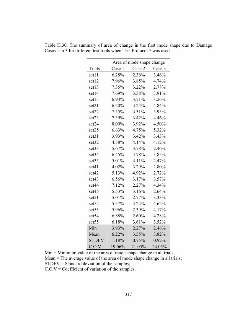
317
Table H.30. The summary of area of change in the first mode shape due to Damage Cases 1 to 3 for different test trials when Test Protocol 7 was used.
Area of mode shape change Trials Case 1 Case 2 Case 3 set11 6.28% 2.36% 3.46% set12 7.96% 3.85% 4.74% set13 7.35% 3.22% 2.78% set14 7.69% 3.38% 3.91% set15 6.94% 3.71% 3.26% set21 6.20% 3.24% 4.84% set22 7.55% 4.31% 5.95% set23 7.39% 3.42% 4.46% set24 8.00% 3.92% 4.50% set25 6.63% 4.75% 5.32% set31 3.93% 3.42% 3.43% set32 4.38% 4.14% 4.12% set33 5.67% 3.78% 2.46% set34 6.45% 4.78% 3.85% set35 5.01% 4.11% 2.47% set41 4.02% 3.29% 2.80% set42 5.13% 4.92% 2.72% set43 6.56% 3.17% 3.57% set44 7.12% 2.27% 4.34% set45 5.53% 3.16% 2.64% set51 5.01% 2.77% 3.33% set52 5.57% 4.24% 4.62% set53 5.96% 2.39% 4.17% set54 6.88% 2.60% 4.28% set55 6.18% 3.61% 3.52% Min 3.93% 2.27% 2.46% Mean 6.22% 3.55% 3.82% STDEV 1.18% 0.75% 0.92% C.O.V 19.06% 21.05% 24.05%
Min = Minimum value of the area of mode shape change in all trials; Mean = The average value of the area of mode shape change in all trials; STDEV = Standard deviation of the samples; C.O.V = Coefficient of variation of the samples.

318
Table H.31. The summary of area of change in the first mode shape due to Damage Cases 4 to 9 for different test trials when Test Protocol 7 was used.
Area of mode shape change Trials Case 4 Case 5 Case 6 Case 7 Case 8 Case 9 set11 5.76% 3.47% 2.64% 3.40% 4.54% 4.58% set12 4.15% 3.53% 3.87% 4.30% 4.26% 3.36% set13 4.42% 2.87% 3.35% 2.93% 4.76% 4.67% set14 3.28% 4.13% 3.42% 4.14% 4.24% 4.86% set15 4.14% 2.68% 2.98% 4.35% 3.25% 3.21% set21 6.06% 4.11% 3.00% 3.09% 3.61% 5.29% set22 4.84% 4.31% 4.71% 3.93% 3.70% 3.26% set23 5.12% 3.42% 4.51% 3.59% 5.14% 5.04% set24 3.94% 4.24% 4.37% 4.65% 3.89% 5.45% set25 5.28% 4.19% 4.00% 4.41% 3.55% 3.78% set31 4.43% 3.90% 3.84% 4.24% 3.84% 4.88% set32 3.53% 4.61% 3.49% 3.90% 2.69% 3.72% set33 3.87% 3.45% 4.68% 4.61% 4.47% 4.50% set34 3.36% 3.91% 4.78% 3.79% 3.71% 4.54% set35 3.55% 3.96% 4.97% 4.00% 4.02% 3.25% set41 4.87% 3.50% 3.18% 3.35% 3.45% 3.69% set42 5.11% 3.54% 3.75% 2.76% 2.97% 3.67% set43 4.42% 3.58% 3.37% 2.99% 3.83% 4.82% set44 3.53% 3.87% 4.42% 2.57% 3.08% 5.54% set45 4.25% 3.97% 3.10% 4.26% 2.05% 3.09% set51 5.13% 3.34% 2.82% 3.53% 3.87% 3.89% set52 3.49% 3.49% 3.78% 3.71% 3.13% 3.33% set53 4.42% 3.44% 3.28% 2.82% 3.92% 5.28% set54 2.47% 3.75% 3.89% 3.40% 4.14% 5.70% set55 4.07% 2.72% 2.97% 4.47% 2.77% 3.07% Min 2.47% 2.68% 2.64% 2.57% 2.05% 3.07% Mean 4.30% 3.68% 3.73% 3.73% 3.71% 4.26% STDEV 0.84% 0.48% 0.68% 0.62% 0.70% 0.87% C.O.V 19.55% 13.08% 18.30% 16.74% 18.78% 20.47%
Min = Minimum value of the area of mode shape change in all trials; Mean = The average value of the area of mode shape change in all trials; STDEV = Standard deviation of the samples; C.O.V = Coefficient of variation of the samples.

319
Table H.32. The summary of area of change in the first mode shape due to Damage Cases 10 to 15 for different test trials when Test Protocol 7 was used.
Area of mode shape change Trials Case 10 Case 11 Case 12 Case 13 Case 14 Case 15 set11 3.91% 4.25% 3.87% 3.87% 4.54% 3.95% set12 4.40% 3.96% 2.83% 2.65% 3.16% 3.80% set13 7.32% 3.45% 3.99% 3.95% 3.34% 5.23% set14 4.05% 5.60% 3.73% 5.27% 4.59% 4.77% set15 5.16% 2.93% 3.61% 3.63% 4.70% 3.69% set21 4.91% 5.06% 4.46% 4.35% 4.02% 3.69% set22 4.47% 3.66% 4.14% 2.92% 2.72% 5.41% set23 5.47% 4.18% 4.96% 4.25% 2.38% 4.26% set24 4.29% 5.35% 4.17% 5.54% 2.86% 4.05% set25 4.13% 4.91% 4.61% 3.27% 3.06% 3.17% set31 5.46% 5.53% 3.56% 5.42% 4.25% 2.16% set32 4.66% 7.43% 4.28% 4.50% 4.25% 3.28% set33 7.83% 5.75% 4.14% 4.58% 3.25% 4.01% set34 5.76% 4.48% 3.52% 5.12% 4.48% 2.71% set35 6.11% 4.67% 3.61% 3.96% 2.68% 2.68% set41 5.70% 3.28% 4.83% 4.97% 4.34% 2.48% set42 5.27% 4.39% 4.47% 4.66% 6.10% 3.65% set43 8.06% 3.03% 4.24% 5.41% 4.21% 2.88% set44 6.57% 4.44% 4.58% 4.18% 3.86% 3.17% set45 6.59% 3.29% 4.02% 4.31% 4.20% 3.30% set51 3.90% 4.64% 3.63% 5.11% 4.12% 2.25% set52 3.93% 5.86% 3.53% 4.39% 4.37% 2.69% set53 6.27% 4.28% 4.52% 4.75% 3.50% 4.31% set54 3.90% 3.51% 4.39% 5.41% 3.69% 3.70% set55 4.66% 4.03% 4.12% 3.13% 3.41% 3.33% Min 3.90% 2.93% 2.83% 2.65% 2.38% 2.16% Mean 5.31% 4.48% 4.07% 4.38% 3.84% 3.55% STDEV 1.25% 1.05% 0.49% 0.82% 0.82% 0.85% C.O.V 23.56% 23.53% 12.09% 18.73% 21.37% 24.08%
Min = Minimum value of the area of mode shape change in all trials; Mean = The average value of the area of mode shape change in all trials; STDEV = Standard deviation of the samples; C.O.V = Coefficient of variation of the samples.
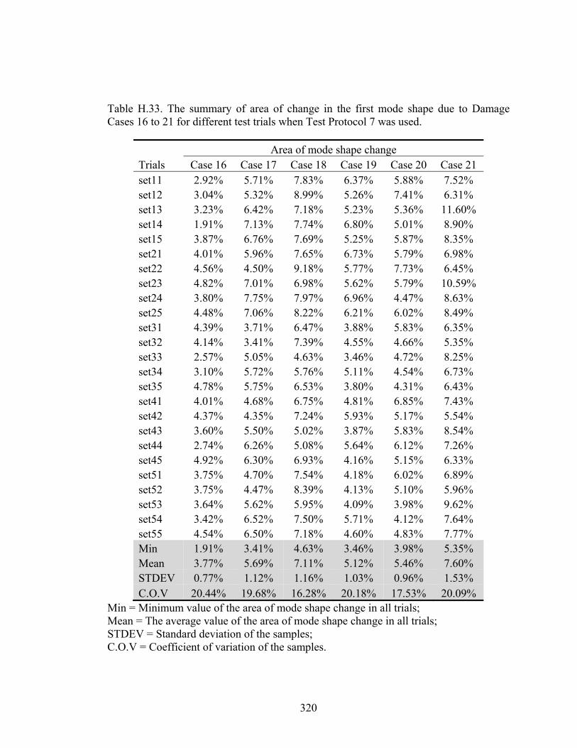
320
Table H.33. The summary of area of change in the first mode shape due to Damage Cases 16 to 21 for different test trials when Test Protocol 7 was used.
Area of mode shape change Trials Case 16 Case 17 Case 18 Case 19 Case 20 Case 21 set11 2.92% 5.71% 7.83% 6.37% 5.88% 7.52% set12 3.04% 5.32% 8.99% 5.26% 7.41% 6.31% set13 3.23% 6.42% 7.18% 5.23% 5.36% 11.60% set14 1.91% 7.13% 7.74% 6.80% 5.01% 8.90% set15 3.87% 6.76% 7.69% 5.25% 5.87% 8.35% set21 4.01% 5.96% 7.65% 6.73% 5.79% 6.98% set22 4.56% 4.50% 9.18% 5.77% 7.73% 6.45% set23 4.82% 7.01% 6.98% 5.62% 5.79% 10.59% set24 3.80% 7.75% 7.97% 6.96% 4.47% 8.63% set25 4.48% 7.06% 8.22% 6.21% 6.02% 8.49% set31 4.39% 3.71% 6.47% 3.88% 5.83% 6.35% set32 4.14% 3.41% 7.39% 4.55% 4.66% 5.35% set33 2.57% 5.05% 4.63% 3.46% 4.72% 8.25% set34 3.10% 5.72% 5.76% 5.11% 4.54% 6.73% set35 4.78% 5.75% 6.53% 3.80% 4.31% 6.43% set41 4.01% 4.68% 6.75% 4.81% 6.85% 7.43% set42 4.37% 4.35% 7.24% 5.93% 5.17% 5.54% set43 3.60% 5.50% 5.02% 3.87% 5.83% 8.54% set44 2.74% 6.26% 5.08% 5.64% 6.12% 7.26% set45 4.92% 6.30% 6.93% 4.16% 5.15% 6.33% set51 3.75% 4.70% 7.54% 4.18% 6.02% 6.89% set52 3.75% 4.47% 8.39% 4.13% 5.10% 5.96% set53 3.64% 5.62% 5.95% 4.09% 3.98% 9.62% set54 3.42% 6.52% 7.50% 5.71% 4.12% 7.64% set55 4.54% 6.50% 7.18% 4.60% 4.83% 7.77% Min 1.91% 3.41% 4.63% 3.46% 3.98% 5.35% Mean 3.77% 5.69% 7.11% 5.12% 5.46% 7.60% STDEV 0.77% 1.12% 1.16% 1.03% 0.96% 1.53% C.O.V 20.44% 19.68% 16.28% 20.18% 17.53% 20.09%
Min = Minimum value of the area of mode shape change in all trials; Mean = The average value of the area of mode shape change in all trials; STDEV = Standard deviation of the samples; C.O.V = Coefficient of variation of the samples.
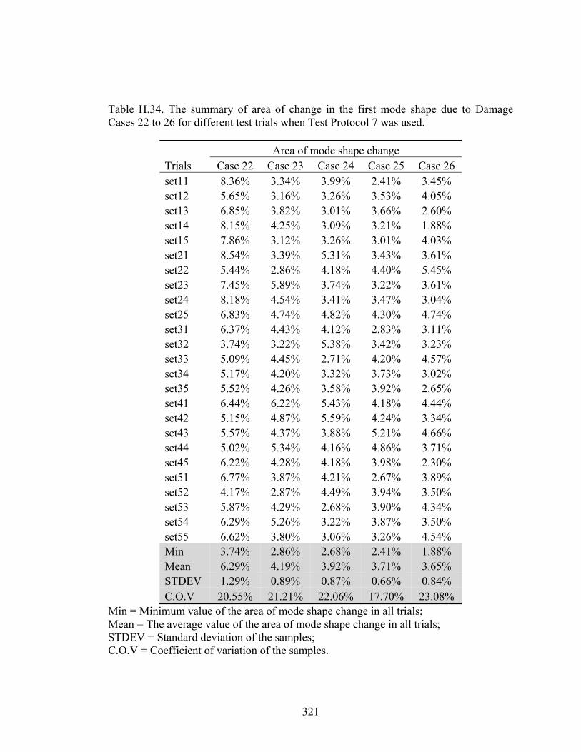
321
Table H.34. The summary of area of change in the first mode shape due to Damage Cases 22 to 26 for different test trials when Test Protocol 7 was used.
Area of mode shape change Trials Case 22 Case 23 Case 24 Case 25 Case 26 set11 8.36% 3.34% 3.99% 2.41% 3.45% set12 5.65% 3.16% 3.26% 3.53% 4.05% set13 6.85% 3.82% 3.01% 3.66% 2.60% set14 8.15% 4.25% 3.09% 3.21% 1.88% set15 7.86% 3.12% 3.26% 3.01% 4.03% set21 8.54% 3.39% 5.31% 3.43% 3.61% set22 5.44% 2.86% 4.18% 4.40% 5.45% set23 7.45% 5.89% 3.74% 3.22% 3.61% set24 8.18% 4.54% 3.41% 3.47% 3.04% set25 6.83% 4.74% 4.82% 4.30% 4.74% set31 6.37% 4.43% 4.12% 2.83% 3.11% set32 3.74% 3.22% 5.38% 3.42% 3.23% set33 5.09% 4.45% 2.71% 4.20% 4.57% set34 5.17% 4.20% 3.32% 3.73% 3.02% set35 5.52% 4.26% 3.58% 3.92% 2.65% set41 6.44% 6.22% 5.43% 4.18% 4.44% set42 5.15% 4.87% 5.59% 4.24% 3.34% set43 5.57% 4.37% 3.88% 5.21% 4.66% set44 5.02% 5.34% 4.16% 4.86% 3.71% set45 6.22% 4.28% 4.18% 3.98% 2.30% set51 6.77% 3.87% 4.21% 2.67% 3.89% set52 4.17% 2.87% 4.49% 3.94% 3.50% set53 5.87% 4.29% 2.68% 3.90% 4.34% set54 6.29% 5.26% 3.22% 3.87% 3.50% set55 6.62% 3.80% 3.06% 3.26% 4.54% Min 3.74% 2.86% 2.68% 2.41% 1.88% Mean 6.29% 4.19% 3.92% 3.71% 3.65% STDEV 1.29% 0.89% 0.87% 0.66% 0.84% C.O.V 20.55% 21.21% 22.06% 17.70% 23.08%
Min = Minimum value of the area of mode shape change in all trials; Mean = The average value of the area of mode shape change in all trials; STDEV = Standard deviation of the samples; C.O.V = Coefficient of variation of the samples.

322
Table H.35. The summary of area of change in the first mode shape due to Damage Cases 1 to 3 for different test trials when Test Protocol 8 was used.
Area of mode shape change Trials Case 1 Case 2 Case 3 set11 8.14% 4.13% 5.49% set12 7.80% 5.73% 3.96% set13 8.75% 7.03% 5.08% set14 10.98% 6.31% 5.98% set15 6.31% 6.75% 4.76% set21 10.39% 6.20% 6.39% set22 8.78% 8.18% 6.93% set23 10.05% 8.13% 6.87% set24 12.54% 7.18% 7.07% set25 7.31% 8.94% 8.81% set31 7.16% 4.38% 7.49% set32 7.58% 9.21% 5.26% set33 7.80% 7.91% 6.44% set34 9.86% 6.90% 5.97% set35 5.56% 8.22% 7.21% set41 9.16% 6.02% 5.86% set42 8.42% 7.67% 6.24% set43 9.30% 5.41% 6.16% set44 10.08% 7.62% 6.14% set45 6.53% 8.60% 5.45% set51 8.33% 5.84% 5.27% set52 8.79% 7.22% 7.31% set53 8.70% 8.14% 7.08% set54 10.74% 5.06% 8.58% set55 6.90% 5.99% 6.58% Min 5.56% 4.13% 3.96% Mean 8.64% 6.91% 6.34% STDEV 1.63% 1.38% 1.12% C.O.V 18.88% 19.97% 17.67%
Min = Minimum value of the area of mode shape change in all trials; Mean = The average value of the area of mode shape change in all trials; STDEV = Standard deviation of the samples; C.O.V = Coefficient of variation of the samples.

323
Table H.36. The summary of area of change in the first mode shape due to Damage Cases 4 to 9 for different test trials when Test Protocol 8 was used.
Area of mode shape change Trials Case 4 Case 5 Case 6 Case 7 Case 8 Case 9 set11 6.14% 5.64% 5.14% 7.04% 8.12% 6.72% set12 5.74% 7.25% 6.78% 5.49% 4.45% 6.13% set13 8.04% 4.89% 5.80% 5.24% 10.53% 5.85% set14 4.51% 5.88% 4.15% 7.25% 5.81% 9.29% set15 6.29% 5.37% 6.68% 5.77% 6.03% 6.36% set21 5.65% 7.30% 5.30% 7.37% 8.58% 8.35% set22 6.23% 7.01% 8.59% 7.21% 8.18% 6.46% set23 8.13% 6.11% 7.03% 5.83% 11.98% 6.58% set24 5.84% 6.80% 5.84% 7.86% 5.78% 10.33% set25 5.47% 6.43% 6.68% 7.43% 6.20% 6.35% set31 6.78% 6.37% 6.29% 9.26% 8.40% 8.86% set32 5.92% 8.42% 7.77% 5.64% 5.83% 7.55% set33 7.12% 6.17% 7.69% 6.92% 11.76% 7.04% set34 5.91% 6.45% 5.29% 7.12% 7.46% 11.90% set35 4.79% 6.16% 7.31% 8.12% 6.20% 7.33% set41 6.13% 8.00% 6.49% 6.71% 8.74% 8.48% set42 6.43% 6.75% 5.82% 7.01% 5.11% 4.68% set43 8.47% 6.39% 5.49% 5.12% 10.65% 7.51% set44 6.12% 8.55% 6.03% 8.27% 5.65% 11.36% set45 6.61% 6.02% 6.69% 8.34% 7.08% 8.00% set51 7.33% 5.37% 3.90% 6.42% 5.98% 7.11% set52 6.83% 5.64% 7.94% 5.07% 7.27% 6.67% set53 6.93% 5.23% 8.49% 6.52% 8.89% 5.57% set54 5.87% 5.40% 4.63% 5.89% 6.53% 8.61% set55 7.67% 4.60% 4.46% 6.02% 4.77% 3.98% Min 4.51% 4.60% 3.90% 5.07% 4.45% 3.98% Mean 6.44% 6.33% 6.25% 6.76% 7.44% 7.48% STDEV 0.98% 1.02% 1.30% 1.11% 2.11% 1.89% C.O.V 15.18% 16.17% 20.75% 16.47% 28.39% 25.21%
Min = Minimum value of the area of mode shape change in all trials; Mean = The average value of the area of mode shape change in all trials; STDEV = Standard deviation of the samples; C.O.V = Coefficient of variation of the samples.

324
Table H.37. The summary of area of change in the first mode shape due to Damage Cases 10 to 15 for different test trials when Test Protocol 8 was used.
Area of mode shape change Trials Case 10 Case 11 Case 12 Case 13 Case 14 Case 15 set11 7.41% 8.77% 5.56% 6.58% 6.57% 7.83% set12 6.94% 7.71% 6.38% 6.90% 7.71% 7.01% set13 6.30% 8.96% 6.76% 7.30% 8.14% 5.03% set14 7.55% 10.37% 8.80% 5.64% 9.33% 6.21% set15 7.80% 5.78% 8.71% 7.79% 8.95% 4.59% set21 9.41% 9.83% 5.29% 7.87% 6.19% 7.12% set22 8.30% 6.93% 5.95% 5.92% 8.19% 8.97% set23 7.06% 8.43% 6.44% 5.71% 7.19% 7.92% set24 6.27% 9.74% 6.81% 7.01% 7.41% 7.76% set25 7.81% 5.12% 7.52% 7.27% 8.01% 6.15% set31 7.96% 9.21% 6.74% 6.14% 6.57% 6.98% set32 6.80% 6.49% 5.08% 7.78% 7.02% 8.03% set33 6.82% 6.34% 8.05% 6.75% 6.55% 5.93% set34 8.75% 8.15% 7.81% 5.39% 7.07% 7.92% set35 9.08% 6.76% 7.52% 10.31% 8.79% 3.27% set41 10.04% 8.99% 6.17% 8.06% 5.91% 7.92% set42 9.78% 7.78% 7.75% 8.19% 6.69% 9.25% set43 10.00% 5.87% 8.01% 5.74% 6.53% 6.30% set44 9.58% 7.13% 9.08% 8.13% 7.55% 8.24% set45 10.88% 10.03% 6.97% 9.38% 8.94% 5.99% set51 5.99% 8.62% 6.83% 6.35% 8.00% 7.86% set52 5.14% 8.35% 7.36% 8.09% 8.59% 7.60% set53 6.11% 7.52% 8.39% 6.34% 9.06% 6.91% set54 8.73% 8.21% 8.32% 6.56% 8.41% 6.75% set55 8.45% 9.79% 8.56% 9.90% 4.44% 5.67% Min 5.14% 5.12% 5.08% 5.39% 4.44% 3.27% Mean 7.96% 8.04% 7.23% 7.24% 7.51% 6.93% STDEV 1.50% 1.45% 1.13% 1.32% 1.18% 1.38% C.O.V 18.79% 18.07% 15.63% 18.17% 15.72% 19.92%
Min = Minimum value of the area of mode shape change in all trials; Mean = The average value of the area of mode shape change in all trials; STDEV = Standard deviation of the samples; C.O.V = Coefficient of variation of the samples.

325
Table H.38. The summary of area of change in the first mode shape due to Damage Cases 16 to 21 for different test trials when Test Protocol 8 was used.
Area of mode shape change Trials Case 16 Case 17 Case 18 Case 19 Case 20 Case 21 set11 8.31% 7.81% 7.34% 7.86% 6.59% 7.13% set12 6.74% 7.58% 9.12% 7.45% 9.62% 5.69% set13 6.89% 10.71% 7.75% 5.08% 6.80% 8.12% set14 6.06% 7.15% 10.43% 6.81% 6.64% 9.43% set15 8.77% 7.68% 8.47% 6.09% 4.88% 9.96% set21 8.10% 9.79% 9.60% 8.82% 8.84% 9.04% set22 7.81% 9.59% 10.56% 10.13% 10.91% 7.46% set23 6.52% 12.26% 9.40% 5.99% 7.56% 10.40% set24 8.85% 9.44% 12.18% 9.38% 9.42% 11.87% set25 8.29% 8.58% 9.85% 7.41% 6.27% 11.50% set31 5.42% 7.78% 6.35% 7.24% 7.33% 6.00% set32 6.91% 7.00% 8.42% 7.47% 8.40% 5.32% set33 6.03% 10.65% 7.66% 5.15% 6.84% 7.66% set34 7.31% 7.39% 9.34% 7.06% 8.59% 10.32% set35 7.71% 6.47% 7.50% 6.09% 4.28% 9.08% set41 9.08% 9.00% 7.95% 9.98% 10.03% 9.38% set42 8.00% 9.67% 10.21% 9.80% 10.22% 8.40% set43 7.77% 11.48% 7.78% 6.59% 8.56% 10.55% set44 6.74% 9.37% 9.89% 9.24% 9.40% 10.59% set45 8.39% 9.61% 9.15% 7.32% 6.41% 9.77% set51 7.62% 7.07% 6.47% 7.31% 8.55% 7.45% set52 7.04% 9.02% 8.84% 9.17% 10.20% 5.80% set53 4.90% 9.88% 6.61% 5.51% 8.42% 9.02% set54 6.19% 7.28% 9.91% 7.90% 8.97% 10.37% set55 7.07% 7.11% 7.31% 7.64% 5.66% 9.92% Min 4.90% 6.47% 6.35% 5.08% 4.28% 5.32% Mean 7.30% 8.78% 8.72% 7.54% 7.98% 8.81% STDEV 1.08% 1.55% 1.45% 1.48% 1.75% 1.85% C.O.V 14.84% 17.62% 16.66% 19.69% 21.97% 20.95%
Min = Minimum value of the area of mode shape change in all trials; Mean = The average value of the area of mode shape change in all trials; STDEV = Standard deviation of the samples; C.O.V = Coefficient of variation of the samples.

326
Table H.39. The summary of area of change in the first mode shape due to Damage Cases 22 to 26 for different test trials when Test Protocol 8 was used.
Area of mode shape change Trials Case 22 Case 23 Case 24 Case 25 Case 26 set11 9.49% 5.84% 6.72% 6.12% 6.65% set12 7.84% 4.57% 7.82% 7.51% 6.18% set13 9.94% 6.10% 6.40% 4.74% 6.12% set14 9.81% 4.84% 7.39% 6.04% 5.36% set15 6.64% 7.39% 7.71% 5.59% 7.28% set21 11.85% 5.05% 7.26% 7.64% 6.33% set22 9.61% 5.79% 8.18% 6.84% 7.83% set23 10.22% 4.34% 6.69% 5.90% 6.66% set24 11.99% 5.79% 8.17% 7.08% 6.83% set25 8.86% 8.04% 8.69% 6.31% 7.64% set31 9.05% 7.16% 6.78% 6.76% 8.46% set32 7.40% 3.81% 7.17% 8.43% 7.01% set33 8.97% 5.80% 6.61% 5.78% 6.42% set34 10.16% 5.30% 7.66% 5.39% 6.08% set35 5.88% 5.69% 7.14% 5.25% 7.67% set41 9.78% 6.19% 6.00% 7.36% 8.76% set42 8.20% 5.81% 7.23% 9.07% 6.05% set43 8.88% 7.66% 7.23% 6.86% 6.33% set44 10.24% 4.36% 8.06% 7.18% 5.85% set45 8.15% 6.69% 8.00% 5.92% 9.09% set51 10.19% 8.44% 5.96% 7.15% 7.69% set52 8.35% 4.64% 8.66% 8.53% 8.29% set53 9.94% 6.03% 7.26% 6.25% 6.57% set54 10.07% 5.81% 7.36% 6.06% 5.16% set55 7.32% 7.93% 7.39% 6.47% 7.22% Min 5.88% 3.81% 5.96% 4.74% 5.16% Mean 9.15% 5.96% 7.34% 6.65% 6.94% STDEV 1.46% 1.25% 0.73% 1.06% 1.03% C.O.V 15.91% 20.98% 9.92% 15.97% 14.88%
Min = Minimum value of the area of mode shape change in all trials; Mean = The average value of the area of mode shape change in all trials; STDEV = Standard deviation of the samples; C.O.V = Coefficient of variation of the samples.

327
Figure H.1. Comparison of Normal distributions of the area of mode shape change forthe undamaged group of 170 pairs and the damaged group of 25 data pairs for DamageCase: (a) 4, (b) 5, and (c) 6, when the Test Protocol 1 was used.
(a)
(b)
(c)
0.01 0 0.01 0.02 0.03 0.04 0.05 0.06 0.07 0.08 0.09 0.10
200
400
600
800
The area of mode shape change
Dis
trib
utio
n de
nsit
y
0.01 0 0.01 0.02 0.03 0.04 0.05 0.06 0.07 0.08 0.09 0.10
200
400
600
800
The area of mode shape change
Dis
trib
utio
n de
nsit
y
0.01 0 0.01 0.02 0.03 0.04 0.05 0.06 0.07 0.08 0.09 0.10
200
400
600
800
Distribution of undamaged groupDistribution of damaged group90th percentile of undamaged group95th percentile of undamaged group
The area of mode shape change
Dis
trib
utio
n de
nsit
y
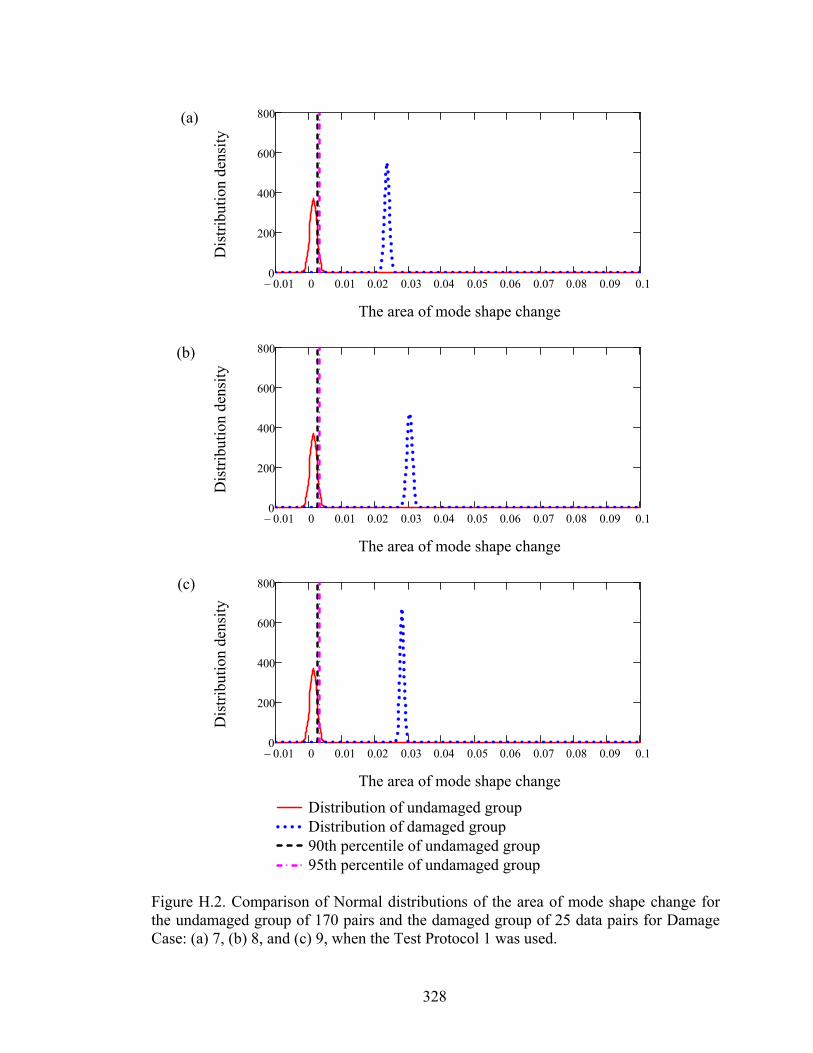
328
Figure H.2. Comparison of Normal distributions of the area of mode shape change forthe undamaged group of 170 pairs and the damaged group of 25 data pairs for DamageCase: (a) 7, (b) 8, and (c) 9, when the Test Protocol 1 was used.
(a)
(b)
(c)
0.01 0 0.01 0.02 0.03 0.04 0.05 0.06 0.07 0.08 0.09 0.10
200
400
600
800
The area of mode shape change
Dis
trib
utio
n de
nsit
y
0.01 0 0.01 0.02 0.03 0.04 0.05 0.06 0.07 0.08 0.09 0.10
200
400
600
800
The area of mode shape change
Dis
trib
utio
n de
nsit
y
0.01 0 0.01 0.02 0.03 0.04 0.05 0.06 0.07 0.08 0.09 0.10
200
400
600
800
Distribution of undamaged groupDistribution of damaged group90th percentile of undamaged group95th percentile of undamaged group
The area of mode shape change
Dis
trib
utio
n de
nsit
y

329
Figure H.3. Comparison of Normal distributions of the area of mode shape change forthe undamaged group of 170 pairs and the damaged group of 25 data pairs for DamageCase: (a) 10, (b) 11, and (c) 12, when the Test Protocol 1 was used.
(a)
(b)
(c)
0.01 0 0.01 0.02 0.03 0.04 0.05 0.06 0.07 0.08 0.09 0.10
200
400
600
800
The area of mode shape change
Dis
trib
utio
n de
nsit
y
0.01 0 0.01 0.02 0.03 0.04 0.05 0.06 0.07 0.08 0.09 0.10
200
400
600
800
The area of mode shape change
Dis
trib
utio
n de
nsit
y
0.01 0 0.01 0.02 0.03 0.04 0.05 0.06 0.07 0.08 0.09 0.10
200
400
600
800
Distribution of undamaged groupDistribution of damaged group90th percentile of undamaged group95th percentile of undamaged group
The area of mode shape change
Dis
trib
utio
n de
nsit
y

330
Figure H.4. Comparison of Normal distributions of the area of mode shape change forthe undamaged group of 170 pairs and the damaged group of 25 data pairs for DamageCase: (a) 13, (b) 14, and (c) 15, when the Test Protocol 1 was used.
(a)
(b)
(c)
0.01 0 0.01 0.02 0.03 0.04 0.05 0.06 0.07 0.08 0.09 0.10
200
400
600
800
The area of mode shape change
Dis
trib
utio
n de
nsit
y
0.01 0 0.01 0.02 0.03 0.04 0.05 0.06 0.07 0.08 0.09 0.10
200
400
600
800
The area of mode shape change
Dis
trib
utio
n de
nsit
y
0.01 0 0.01 0.02 0.03 0.04 0.05 0.06 0.07 0.08 0.09 0.10
200
400
600
800
Distribution of undamaged groupDistribution of damaged group90th percentile of undamaged group95th percentile of undamaged group
The area of mode shape change
Dis
trib
utio
n de
nsit
y
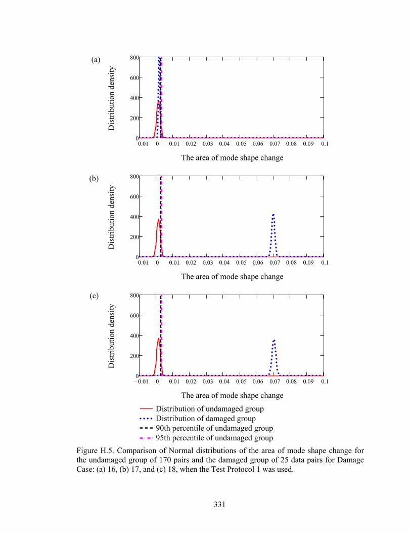
331
Figure H.5. Comparison of Normal distributions of the area of mode shape change forthe undamaged group of 170 pairs and the damaged group of 25 data pairs for DamageCase: (a) 16, (b) 17, and (c) 18, when the Test Protocol 1 was used.
(a)
(b)
(c)
0.01 0 0.01 0.02 0.03 0.04 0.05 0.06 0.07 0.08 0.09 0.10
200
400
600
800
The area of mode shape change
Dis
trib
utio
n de
nsit
y
0.01 0 0.01 0.02 0.03 0.04 0.05 0.06 0.07 0.08 0.09 0.10
200
400
600
800
The area of mode shape change
Dis
trib
utio
n de
nsit
y
0.01 0 0.01 0.02 0.03 0.04 0.05 0.06 0.07 0.08 0.09 0.10
200
400
600
800
Distribution of undamaged groupDistribution of damaged group90th percentile of undamaged group95th percentile of undamaged group
The area of mode shape change
Dis
trib
utio
n de
nsit
y

332
Figure H.6. Comparison of Normal distributions of the area of mode shape change forthe undamaged group of 170 pairs and the damaged group of 25 data pairs for DamageCase: (a) 19, (b) 20, and (c) 21, when the Test Protocol 1 was used.
(a)
(b)
(c)
0.01 0 0.01 0.02 0.03 0.04 0.05 0.06 0.07 0.08 0.09 0.10
200
400
600
800
The area of mode shape change
Dis
trib
utio
n de
nsit
y
0.01 0 0.01 0.02 0.03 0.04 0.05 0.06 0.07 0.08 0.09 0.10
200
400
600
800
The area of mode shape change
Dis
trib
utio
n de
nsit
y
0.01 0 0.01 0.02 0.03 0.04 0.05 0.06 0.07 0.08 0.09 0.10
200
400
600
800
Distribution of undamaged groupDistribution of damaged group90th percentile of undamaged group95th percentile of undamaged group
The area of mode shape change
Dis
trib
utio
n de
nsit
y
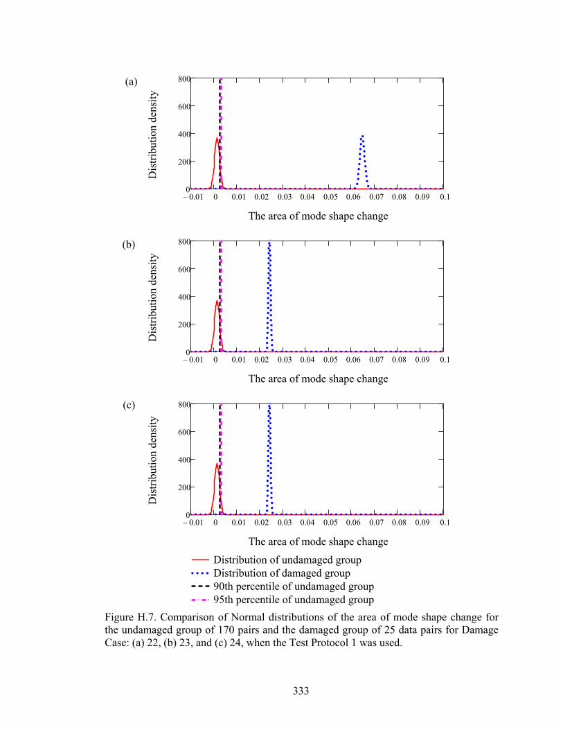
333
Figure H.7. Comparison of Normal distributions of the area of mode shape change forthe undamaged group of 170 pairs and the damaged group of 25 data pairs for DamageCase: (a) 22, (b) 23, and (c) 24, when the Test Protocol 1 was used.
(a)
(b)
(c)
0.01 0 0.01 0.02 0.03 0.04 0.05 0.06 0.07 0.08 0.09 0.10
200
400
600
800
The area of mode shape change
Dis
trib
utio
n de
nsit
y
0.01 0 0.01 0.02 0.03 0.04 0.05 0.06 0.07 0.08 0.09 0.10
200
400
600
800
The area of mode shape change
Dis
trib
utio
n de
nsit
y
0.01 0 0.01 0.02 0.03 0.04 0.05 0.06 0.07 0.08 0.09 0.10
200
400
600
800
Distribution of undamaged groupDistribution of damaged group90th percentile of undamaged group95th percentile of undamaged group
The area of mode shape change
Dis
trib
utio
n de
nsit
y

334
Figure H.8. Comparison of Normal distributions of the area of mode shape change forthe undamaged group of 170 pairs and the damaged group of 25 data pairs for DamageCase: (a) 25 and (b) 26, when the Test Protocol 1 was used.
(a)
(b)
0.01 0 0.01 0.02 0.03 0.04 0.05 0.06 0.07 0.08 0.09 0.10
200
400
600
800
The area of mode shape change
Dis
trib
utio
n de
nsit
y
0.01 0 0.01 0.02 0.03 0.04 0.05 0.06 0.07 0.08 0.09 0.10
200
400
600
800
Distribution of undamaged groupDistribution of damaged group90th percentile of undamaged group95th percentile of undamaged group
The area of mode shape change
Dis
trib
utio
n de
nsit
y

335
Figure H.9. Comparison of Normal distributions of the area of mode shape change forthe undamaged group of 170 pairs and the damaged group of 25 data pairs for DamageCase: (a) 1, (b) 2, and (c) 3, when the Test Protocol 2 was used.
(a)
(b)
(c)
0.01 0 0.01 0.02 0.03 0.04 0.05 0.06 0.07 0.08 0.09 0.10
200
400
600
800
The area of mode shape change
Dis
trib
utio
n de
nsit
y
0.01 0 0.01 0.02 0.03 0.04 0.05 0.06 0.07 0.08 0.09 0.10
200
400
600
800
The area of mode shape change
Dis
trib
utio
n de
nsit
y
0.01 0 0.01 0.02 0.03 0.04 0.05 0.06 0.07 0.08 0.09 0.10
200
400
600
800
Distribution of damaged groupDistribution of undamaged group90th percentile of undamaged group95th percentile of undamaged group
The area of mode shape change
Dis
trib
utio
n de
nsit
y

336
Figure H.10. Comparison of Normal distributions of the area of mode shape change forthe undamaged group of 170 pairs and the damaged group of 25 data pairs for DamageCase: (a) 4, (b) 5, and (c) 6, when the Test Protocol 2 was used.
(a)
(b)
(c)
0.01 0 0.01 0.02 0.03 0.04 0.05 0.06 0.07 0.08 0.09 0.10
200
400
600
800
The area of mode shape change
Dis
trib
utio
n de
nsit
y
0.01 0 0.01 0.02 0.03 0.04 0.05 0.06 0.07 0.08 0.09 0.10
200
400
600
800
The area of mode shape change
Dis
trib
utio
n de
nsit
y
0.01 0 0.01 0.02 0.03 0.04 0.05 0.06 0.07 0.08 0.09 0.10
200
400
600
800
Distribution of damaged groupDistribution of undamaged group90th percentile of undamaged group95th percentile of undamaged group
The area of mode shape change
Dis
trib
utio
n de
nsit
y

337
Figure H.11. Comparison of Normal distributions of the area of mode shape change forthe undamaged group of 170 pairs and the damaged group of 25 data pairs for DamageCase: (a) 7, (b) 8, and (c) 9, when the Test Protocol 2 was used.
(a)
(b)
(c)
0.01 0 0.01 0.02 0.03 0.04 0.05 0.06 0.07 0.08 0.09 0.10
200
400
600
800
The area of mode shape change
Dis
trib
utio
n de
nsit
y
0.01 0 0.01 0.02 0.03 0.04 0.05 0.06 0.07 0.08 0.09 0.10
200
400
600
800
The area of mode shape change
Dis
trib
utio
n de
nsit
y
0.01 0 0.01 0.02 0.03 0.04 0.05 0.06 0.07 0.08 0.09 0.10
200
400
600
800
Distribution of damaged groupDistribution of undamaged group90th percentile of undamaged group95th percentile of undamaged group
The area of mode shape change
Dis
trib
utio
n de
nsit
y
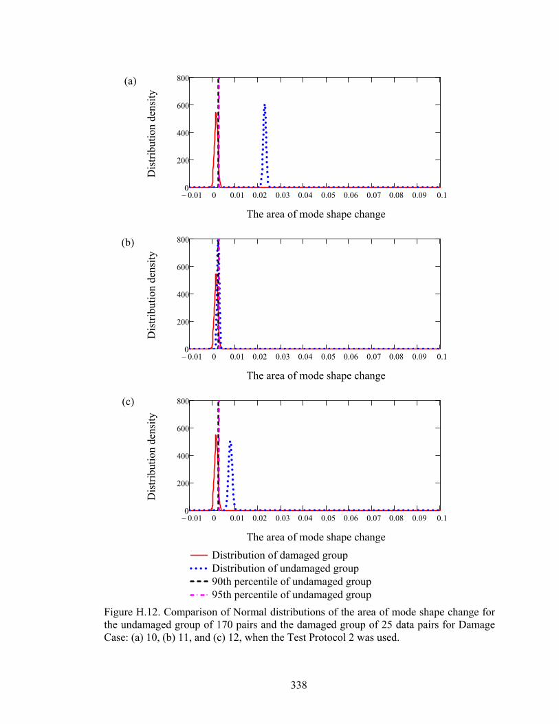
338
Figure H.12. Comparison of Normal distributions of the area of mode shape change forthe undamaged group of 170 pairs and the damaged group of 25 data pairs for DamageCase: (a) 10, (b) 11, and (c) 12, when the Test Protocol 2 was used.
(a)
(b)
(c)
0.01 0 0.01 0.02 0.03 0.04 0.05 0.06 0.07 0.08 0.09 0.10
200
400
600
800
The area of mode shape change
Dis
trib
utio
n de
nsit
y
0.01 0 0.01 0.02 0.03 0.04 0.05 0.06 0.07 0.08 0.09 0.10
200
400
600
800
The area of mode shape change
Dis
trib
utio
n de
nsit
y
0.01 0 0.01 0.02 0.03 0.04 0.05 0.06 0.07 0.08 0.09 0.10
200
400
600
800
Distribution of damaged groupDistribution of undamaged group90th percentile of undamaged group95th percentile of undamaged group
The area of mode shape change
Dis
trib
utio
n de
nsit
y

339
Figure H.13. Comparison of Normal distributions of the area of mode shape change forthe undamaged group of 170 pairs and the damaged group of 25 data pairs for DamageCase: (a) 13, (b) 14, and (c) 15, when the Test Protocol 2 was used.
(a)
(b)
(c)
0.01 0 0.01 0.02 0.03 0.04 0.05 0.06 0.07 0.08 0.09 0.10
200
400
600
800
The area of mode shape change
Dis
trib
utio
n de
nsit
y
0.01 0 0.01 0.02 0.03 0.04 0.05 0.06 0.07 0.08 0.09 0.10
200
400
600
800
The area of mode shape change
Dis
trib
utio
n de
nsit
y
0.01 0 0.01 0.02 0.03 0.04 0.05 0.06 0.07 0.08 0.09 0.10
200
400
600
800
Distribution of damaged groupDistribution of undamaged group90th percentile of undamaged group95th percentile of undamaged group
The area of mode shape change
Dis
trib
utio
n de
nsit
y
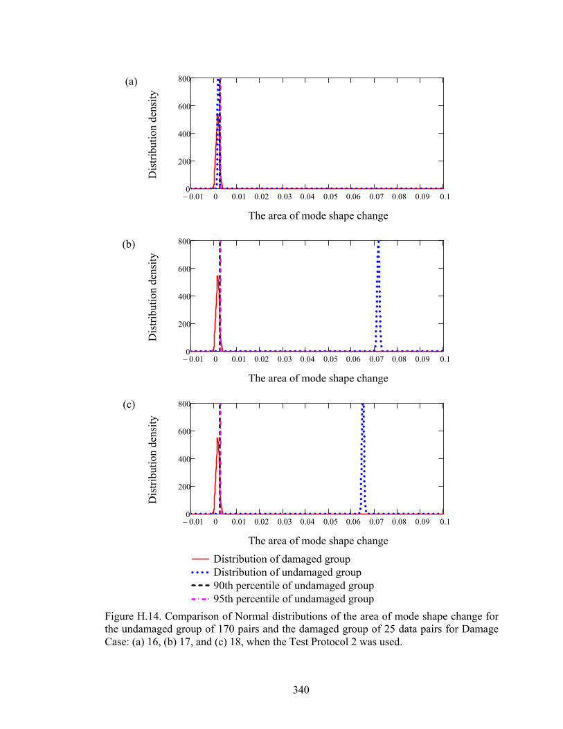
340
Figure H.14. Comparison of Normal distributions of the area of mode shape change forthe undamaged group of 170 pairs and the damaged group of 25 data pairs for DamageCase: (a) 16, (b) 17, and (c) 18, when the Test Protocol 2 was used.
(a)
(b)
(c)
0.01 0 0.01 0.02 0.03 0.04 0.05 0.06 0.07 0.08 0.09 0.10
200
400
600
800
The area of mode shape change
Dis
trib
utio
n de
nsit
y
0.01 0 0.01 0.02 0.03 0.04 0.05 0.06 0.07 0.08 0.09 0.10
200
400
600
800
The area of mode shape change
Dis
trib
utio
n de
nsit
y
0.01 0 0.01 0.02 0.03 0.04 0.05 0.06 0.07 0.08 0.09 0.10
200
400
600
800
Distribution of damaged groupDistribution of undamaged group90th percentile of undamaged group95th percentile of undamaged group
The area of mode shape change
Dis
trib
utio
n de
nsit
y
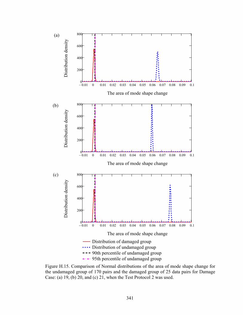
341
Figure H.15. Comparison of Normal distributions of the area of mode shape change forthe undamaged group of 170 pairs and the damaged group of 25 data pairs for DamageCase: (a) 19, (b) 20, and (c) 21, when the Test Protocol 2 was used.
(a)
(b)
(c)
0.01 0 0.01 0.02 0.03 0.04 0.05 0.06 0.07 0.08 0.09 0.10
200
400
600
800
The area of mode shape change
Dis
trib
utio
n de
nsit
y
0.01 0 0.01 0.02 0.03 0.04 0.05 0.06 0.07 0.08 0.09 0.10
200
400
600
800
The area of mode shape change
Dis
trib
utio
n de
nsit
y
0.01 0 0.01 0.02 0.03 0.04 0.05 0.06 0.07 0.08 0.09 0.10
200
400
600
800
Distribution of damaged groupDistribution of undamaged group90th percentile of undamaged group95th percentile of undamaged group
The area of mode shape change
Dis
trib
utio
n de
nsit
y
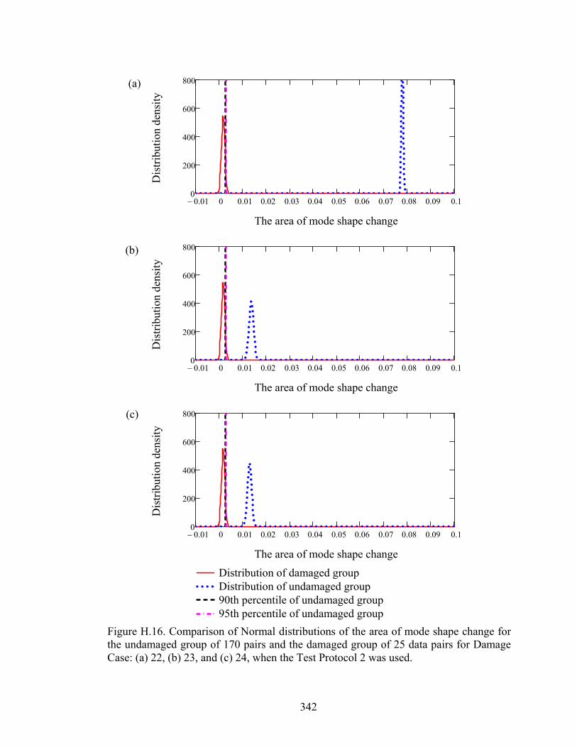
342
Figure H.16. Comparison of Normal distributions of the area of mode shape change forthe undamaged group of 170 pairs and the damaged group of 25 data pairs for DamageCase: (a) 22, (b) 23, and (c) 24, when the Test Protocol 2 was used.
(a)
(b)
(c)
0.01 0 0.01 0.02 0.03 0.04 0.05 0.06 0.07 0.08 0.09 0.10
200
400
600
800
The area of mode shape change
Dis
trib
utio
n de
nsit
y
0.01 0 0.01 0.02 0.03 0.04 0.05 0.06 0.07 0.08 0.09 0.10
200
400
600
800
The area of mode shape change
Dis
trib
utio
n de
nsit
y
0.01 0 0.01 0.02 0.03 0.04 0.05 0.06 0.07 0.08 0.09 0.10
200
400
600
800
Distribution of damaged groupDistribution of undamaged group90th percentile of undamaged group95th percentile of undamaged group
The area of mode shape change
Dis
trib
utio
n de
nsit
y

343
Figure H.17. Comparison of Normal distributions of the area of mode shape change forthe undamaged group of 170 pairs and the damaged group of 25 data pairs for DamageCase: (a) 25 and (b) 26, when the Test Protocol 2 was used.
(a)
(b)
0.01 0 0.01 0.02 0.03 0.04 0.05 0.06 0.07 0.08 0.09 0.10
200
400
600
800
The area of mode shape change
Dis
trib
utio
n de
nsit
y
0.01 0 0.01 0.02 0.03 0.04 0.05 0.06 0.07 0.08 0.09 0.10
200
400
600
800
Distribution of damaged groupDistribution of undamaged group90th percentile of undamaged group95th percentile of undamaged group
The area of mode shape change
Dis
trib
utio
n de
nsit
y
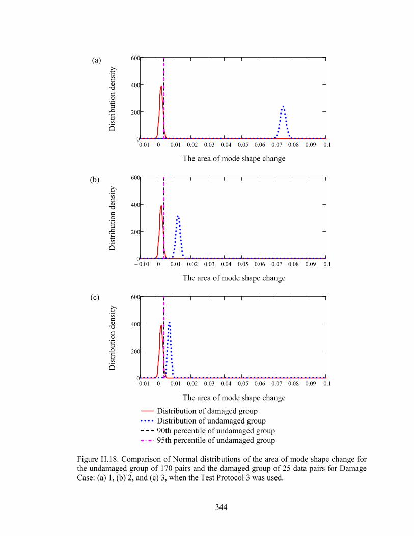
344
Figure H.18. Comparison of Normal distributions of the area of mode shape change forthe undamaged group of 170 pairs and the damaged group of 25 data pairs for DamageCase: (a) 1, (b) 2, and (c) 3, when the Test Protocol 3 was used.
(a)
(b)
(c)
0.01 0 0.01 0.02 0.03 0.04 0.05 0.06 0.07 0.08 0.09 0.10
200
400
600
The area of mode shape change
Dis
trib
utio
n de
nsit
y
0.01 0 0.01 0.02 0.03 0.04 0.05 0.06 0.07 0.08 0.09 0.10
200
400
600
The area of mode shape change
Dis
trib
utio
n de
nsit
y
0.01 0 0.01 0.02 0.03 0.04 0.05 0.06 0.07 0.08 0.09 0.10
200
400
600
Distribution of damaged groupDistribution of undamaged group90th percentile of undamaged group95th percentile of undamaged group
The area of mode shape change
Dis
trib
utio
n de
nsit
y
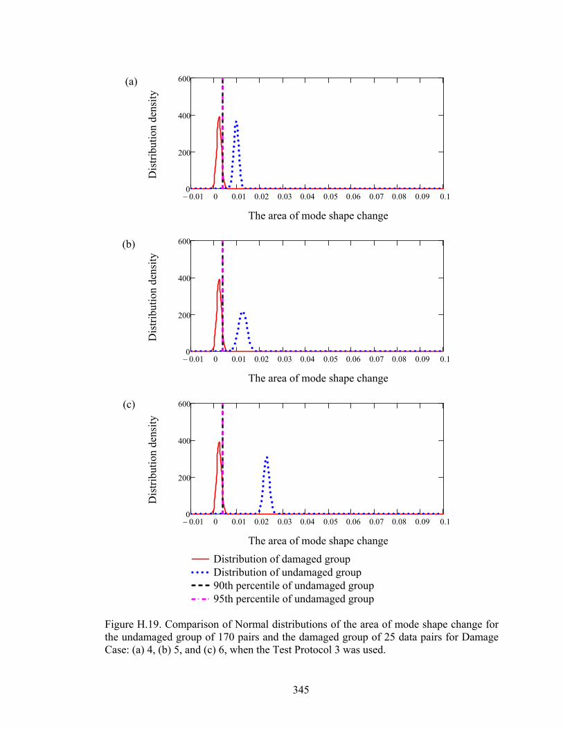
345
Figure H.19. Comparison of Normal distributions of the area of mode shape change forthe undamaged group of 170 pairs and the damaged group of 25 data pairs for DamageCase: (a) 4, (b) 5, and (c) 6, when the Test Protocol 3 was used.
(a)
(b)
(c)
0.01 0 0.01 0.02 0.03 0.04 0.05 0.06 0.07 0.08 0.09 0.10
200
400
600
The area of mode shape change
Dis
trib
utio
n de
nsit
y
0.01 0 0.01 0.02 0.03 0.04 0.05 0.06 0.07 0.08 0.09 0.10
200
400
600
The area of mode shape change
Dis
trib
utio
n de
nsit
y
0.01 0 0.01 0.02 0.03 0.04 0.05 0.06 0.07 0.08 0.09 0.10
200
400
600
Distribution of damaged groupDistribution of undamaged group90th percentile of undamaged group95th percentile of undamaged group
The area of mode shape change
Dis
trib
utio
n de
nsit
y

346
Figure H.20. Comparison of Normal distributions of the area of mode shape change forthe undamaged group of 170 pairs and the damaged group of 25 data pairs for DamageCase: (a) 7, (b) 8, and (c) 9, when the Test Protocol 3 was used.
(a)
(b)
(c)
0.01 0 0.01 0.02 0.03 0.04 0.05 0.06 0.07 0.08 0.09 0.10
200
400
600
The area of mode shape change
Dis
trib
utio
n de
nsit
y
0.01 0 0.01 0.02 0.03 0.04 0.05 0.06 0.07 0.08 0.09 0.10
200
400
600
The area of mode shape change
Dis
trib
utio
n de
nsit
y
0.01 0 0.01 0.02 0.03 0.04 0.05 0.06 0.07 0.08 0.09 0.10
200
400
600
Distribution of damaged groupDistribution of undamaged group90th percentile of undamaged group95th percentile of undamaged group
The area of mode shape change
Dis
trib
utio
n de
nsit
y

347
Figure H.21. Comparison of Normal distributions of the area of mode shape change forthe undamaged group of 170 pairs and the damaged group of 25 data pairs for DamageCase: (a) 10, (b) 11, and (c) 12, when the Test Protocol 3 was used.
(a)
(b)
(c)
0.01 0 0.01 0.02 0.03 0.04 0.05 0.06 0.07 0.08 0.09 0.10
200
400
600
The area of mode shape change
Dis
trib
utio
n de
nsit
y
0.01 0 0.01 0.02 0.03 0.04 0.05 0.06 0.07 0.08 0.09 0.10
200
400
600
The area of mode shape change
Dis
trib
utio
n de
nsit
y
0.01 0 0.01 0.02 0.03 0.04 0.05 0.06 0.07 0.08 0.09 0.10
200
400
600
Distribution of damaged groupDistribution of undamaged group90th percentile of undamaged group95th percentile of undamaged group
The area of mode shape change
Dis
trib
utio
n de
nsit
y

348
Figure H.22. Comparison of Normal distributions of the area of mode shape change forthe undamaged group of 170 pairs and the damaged group of 25 data pairs for DamageCase: (a) 13, (b) 14, and (c) 15, when the Test Protocol 3 was used.
(a)
(b)
(c)
0.01 0 0.01 0.02 0.03 0.04 0.05 0.06 0.07 0.08 0.09 0.10
200
400
600
The area of mode shape change
Dis
trib
utio
n de
nsit
y
0.01 0 0.01 0.02 0.03 0.04 0.05 0.06 0.07 0.08 0.09 0.10
200
400
600
The area of mode shape change
Dis
trib
utio
n de
nsit
y
0.01 0 0.01 0.02 0.03 0.04 0.05 0.06 0.07 0.08 0.09 0.10
200
400
600
Distribution of damaged groupDistribution of undamaged group90th percentile of undamaged group95th percentile of undamaged group
The area of mode shape change
Dis
trib
utio
n de
nsit
y

349
Figure H.23. Comparison of Normal distributions of the area of mode shape change forthe undamaged group of 170 pairs and the damaged group of 25 data pairs for DamageCase: (a) 16, (b) 17, and (c) 18, when the Test Protocol 3 was used.
(a)
(b)
(c)
0.01 0 0.01 0.02 0.03 0.04 0.05 0.06 0.07 0.08 0.09 0.10
200
400
600
The area of mode shape change
Dis
trib
utio
n de
nsit
y
0.01 0 0.01 0.02 0.03 0.04 0.05 0.06 0.07 0.08 0.09 0.10
200
400
600
The area of mode shape change
Dis
trib
utio
n de
nsit
y
0.01 0 0.01 0.02 0.03 0.04 0.05 0.06 0.07 0.08 0.09 0.10
200
400
600
Distribution of damaged groupDistribution of undamaged group90th percentile of undamaged group95th percentile of undamaged group
The area of mode shape change
Dis
trib
utio
n de
nsit
y
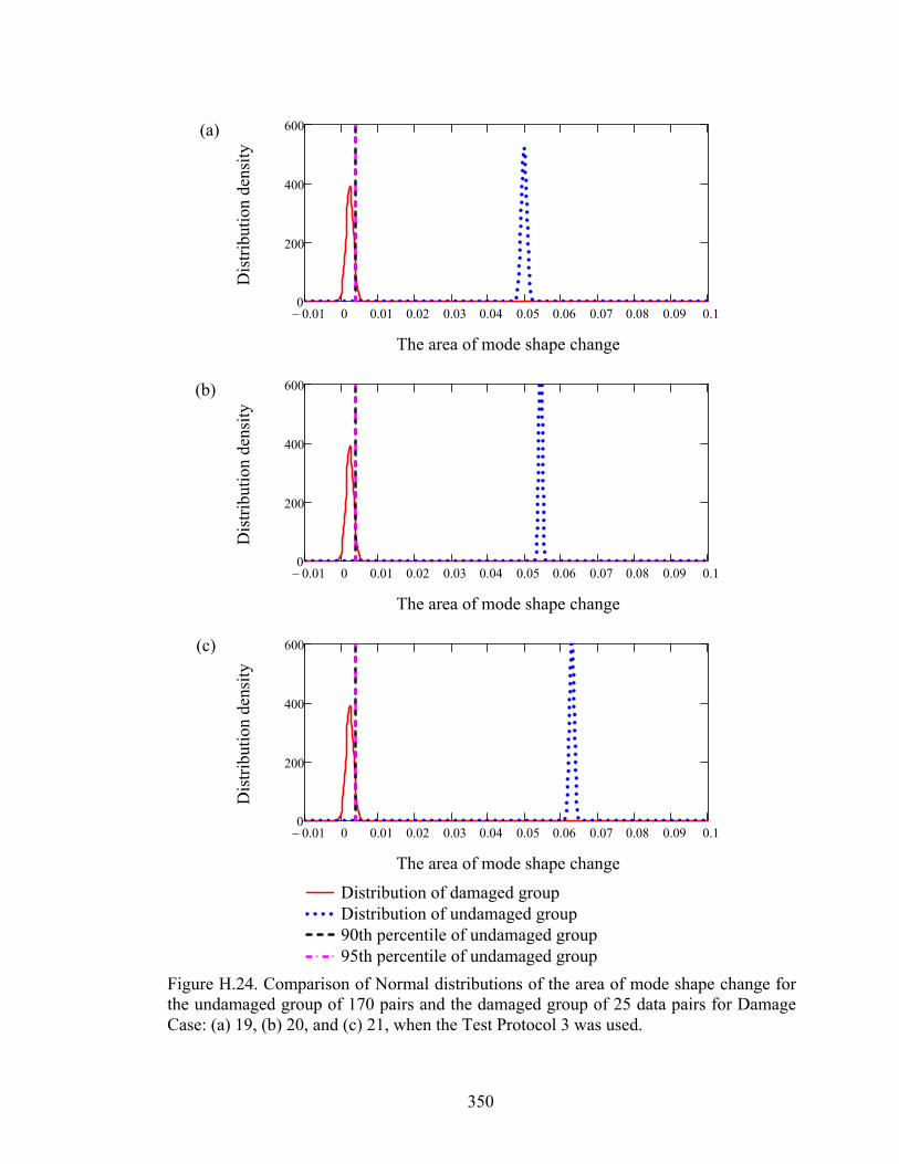
350
Figure H.24. Comparison of Normal distributions of the area of mode shape change forthe undamaged group of 170 pairs and the damaged group of 25 data pairs for DamageCase: (a) 19, (b) 20, and (c) 21, when the Test Protocol 3 was used.
(a)
(b)
(c)
0.01 0 0.01 0.02 0.03 0.04 0.05 0.06 0.07 0.08 0.09 0.10
200
400
600
The area of mode shape change
Dis
trib
utio
n de
nsit
y
0.01 0 0.01 0.02 0.03 0.04 0.05 0.06 0.07 0.08 0.09 0.10
200
400
600
The area of mode shape change
Dis
trib
utio
n de
nsit
y
0.01 0 0.01 0.02 0.03 0.04 0.05 0.06 0.07 0.08 0.09 0.10
200
400
600
Distribution of damaged groupDistribution of undamaged group90th percentile of undamaged group95th percentile of undamaged group
The area of mode shape change
Dis
trib
utio
n de
nsit
y

351
Figure H.25. Comparison of Normal distributions of the area of mode shape change forthe undamaged group of 170 pairs and the damaged group of 25 data pairs for DamageCase: (a) 22, (b) 23, and (c) 24, when the Test Protocol 3 was used.
(a)
(b)
(c)
0.01 0 0.01 0.02 0.03 0.04 0.05 0.06 0.07 0.08 0.09 0.10
200
400
600
The area of mode shape change
Dis
trib
utio
n de
nsit
y
0.01 0 0.01 0.02 0.03 0.04 0.05 0.06 0.07 0.08 0.09 0.10
200
400
600
The area of mode shape change
Dis
trib
utio
n de
nsit
y
0.01 0 0.01 0.02 0.03 0.04 0.05 0.06 0.07 0.08 0.09 0.10
200
400
600
Distribution of damaged groupDistribution of undamaged group90th percentile of undamaged group95th percentile of undamaged group
The area of mode shape change
Dis
trib
utio
n de
nsit
y

352
Figure H.26. Comparison of Normal distributions of the area of mode shape change forthe undamaged group of 170 pairs and the damaged group of 25 data pairs for DamageCase: (a) 25 and (b) 26, when the Test Protocol 3 was used.
(a)
(b)
0.01 0 0.01 0.02 0.03 0.04 0.05 0.06 0.07 0.08 0.09 0.10
200
400
600
The area of mode shape change
Dis
trib
utio
n de
nsit
y
0.01 0 0.01 0.02 0.03 0.04 0.05 0.06 0.07 0.08 0.09 0.10
200
400
600
Distribution of damaged groupDistribution of undamaged group90th percentile of undamaged group95th percentile of undamaged group
The area of mode shape change
Dis
trib
utio
n de
nsit
y
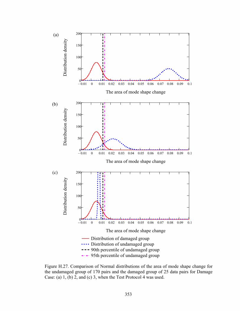
353
Figure H.27. Comparison of Normal distributions of the area of mode shape change forthe undamaged group of 170 pairs and the damaged group of 25 data pairs for DamageCase: (a) 1, (b) 2, and (c) 3, when the Test Protocol 4 was used.
(a)
(b)
(c)
0.01 0 0.01 0.02 0.03 0.04 0.05 0.06 0.07 0.08 0.09 0.10
50
100
150
200
The area of mode shape change
Dis
trib
utio
n de
nsit
y
0.01 0 0.01 0.02 0.03 0.04 0.05 0.06 0.07 0.08 0.09 0.10
50
100
150
200
The area of mode shape change
Dis
trib
utio
n de
nsit
y
0.01 0 0.01 0.02 0.03 0.04 0.05 0.06 0.07 0.08 0.09 0.10
50
100
150
200
Distribution of damaged groupDistribution of undamaged group90th percentile of undamaged group95th percentile of undamaged group
The area of mode shape change
Dis
trib
utio
n de
nsit
y
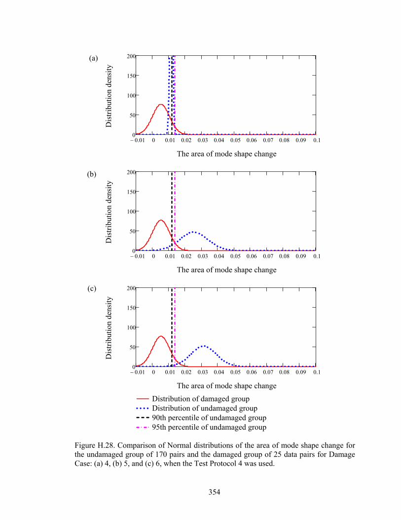
354
Figure H.28. Comparison of Normal distributions of the area of mode shape change forthe undamaged group of 170 pairs and the damaged group of 25 data pairs for DamageCase: (a) 4, (b) 5, and (c) 6, when the Test Protocol 4 was used.
(a)
(b)
(c)
0.01 0 0.01 0.02 0.03 0.04 0.05 0.06 0.07 0.08 0.09 0.10
50
100
150
200
The area of mode shape change
Dis
trib
utio
n de
nsit
y
0.01 0 0.01 0.02 0.03 0.04 0.05 0.06 0.07 0.08 0.09 0.10
50
100
150
200
The area of mode shape change
Dis
trib
utio
n de
nsit
y
0.01 0 0.01 0.02 0.03 0.04 0.05 0.06 0.07 0.08 0.09 0.10
50
100
150
200
Distribution of damaged groupDistribution of undamaged group90th percentile of undamaged group95th percentile of undamaged group
The area of mode shape change
Dis
trib
utio
n de
nsit
y

355
Figure H.29. Comparison of Normal distributions of the area of mode shape change forthe undamaged group of 170 pairs and the damaged group of 25 data pairs for DamageCase: (a) 7, (b) 8, and (c) 9, when the Test Protocol 4 was used.
(a)
(b)
(c)
0.01 0 0.01 0.02 0.03 0.04 0.05 0.06 0.07 0.08 0.09 0.10
50
100
150
200
The area of mode shape change
Dis
trib
utio
n de
nsit
y
0.01 0 0.01 0.02 0.03 0.04 0.05 0.06 0.07 0.08 0.09 0.10
50
100
150
200
The area of mode shape change
Dis
trib
utio
n de
nsit
y
0.01 0 0.01 0.02 0.03 0.04 0.05 0.06 0.07 0.08 0.09 0.10
50
100
150
200
Distribution of damaged groupDistribution of undamaged group90th percentile of undamaged group95th percentile of undamaged group
The area of mode shape change
Dis
trib
utio
n de
nsit
y
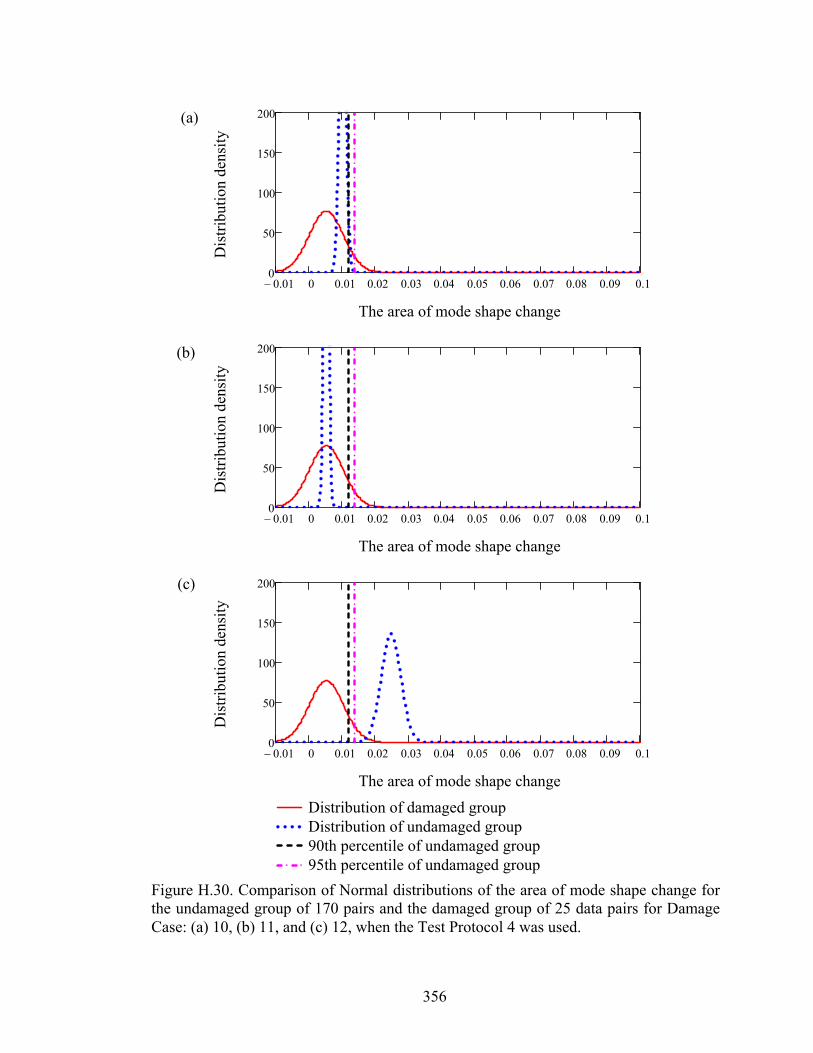
356
Figure H.30. Comparison of Normal distributions of the area of mode shape change forthe undamaged group of 170 pairs and the damaged group of 25 data pairs for DamageCase: (a) 10, (b) 11, and (c) 12, when the Test Protocol 4 was used.
(a)
(b)
(c)
0.01 0 0.01 0.02 0.03 0.04 0.05 0.06 0.07 0.08 0.09 0.10
50
100
150
200
The area of mode shape change
Dis
trib
utio
n de
nsit
y
0.01 0 0.01 0.02 0.03 0.04 0.05 0.06 0.07 0.08 0.09 0.10
50
100
150
200
The area of mode shape change
Dis
trib
utio
n de
nsit
y
0.01 0 0.01 0.02 0.03 0.04 0.05 0.06 0.07 0.08 0.09 0.10
50
100
150
200
Distribution of damaged groupDistribution of undamaged group90th percentile of undamaged group95th percentile of undamaged group
The area of mode shape change
Dis
trib
utio
n de
nsit
y
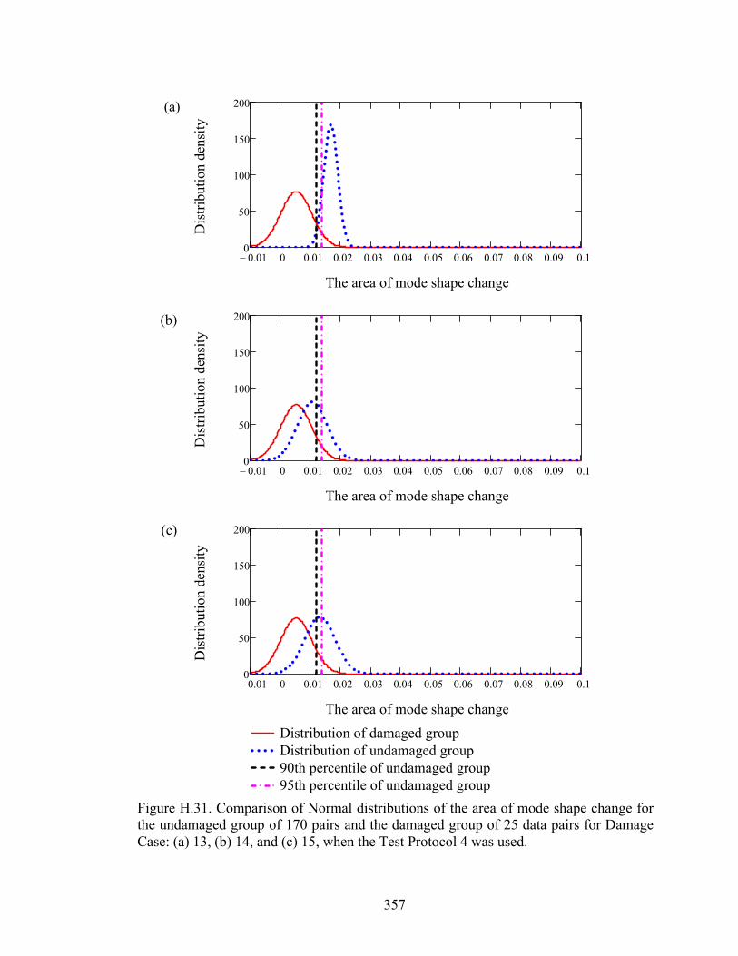
357
Figure H.31. Comparison of Normal distributions of the area of mode shape change forthe undamaged group of 170 pairs and the damaged group of 25 data pairs for DamageCase: (a) 13, (b) 14, and (c) 15, when the Test Protocol 4 was used.
(a)
(b)
(c)
0.01 0 0.01 0.02 0.03 0.04 0.05 0.06 0.07 0.08 0.09 0.10
50
100
150
200
The area of mode shape change
Dis
trib
utio
n de
nsit
y
0.01 0 0.01 0.02 0.03 0.04 0.05 0.06 0.07 0.08 0.09 0.10
50
100
150
200
The area of mode shape change
Dis
trib
utio
n de
nsit
y
0.01 0 0.01 0.02 0.03 0.04 0.05 0.06 0.07 0.08 0.09 0.10
50
100
150
200
Distribution of damaged groupDistribution of undamaged group90th percentile of undamaged group95th percentile of undamaged group
The area of mode shape change
Dis
trib
utio
n de
nsit
y
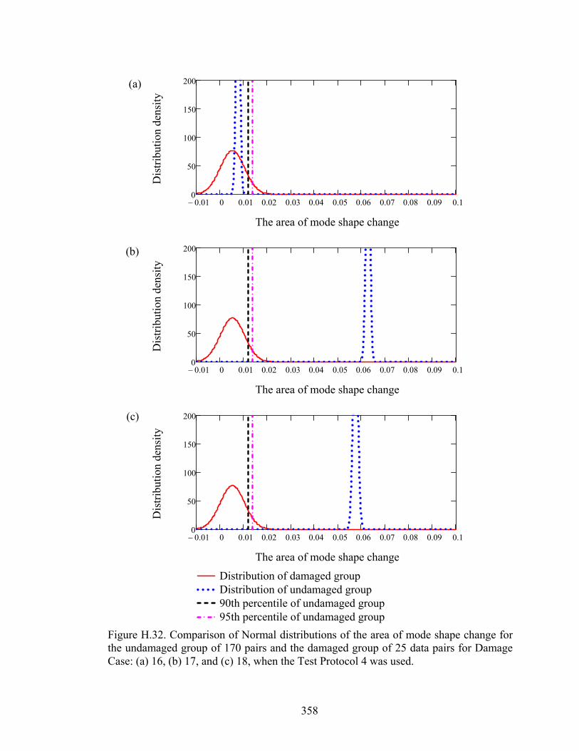
358
Figure H.32. Comparison of Normal distributions of the area of mode shape change forthe undamaged group of 170 pairs and the damaged group of 25 data pairs for DamageCase: (a) 16, (b) 17, and (c) 18, when the Test Protocol 4 was used.
(a)
(b)
(c)
0.01 0 0.01 0.02 0.03 0.04 0.05 0.06 0.07 0.08 0.09 0.10
50
100
150
200
The area of mode shape change
Dis
trib
utio
n de
nsit
y
0.01 0 0.01 0.02 0.03 0.04 0.05 0.06 0.07 0.08 0.09 0.10
50
100
150
200
The area of mode shape change
Dis
trib
utio
n de
nsit
y
0.01 0 0.01 0.02 0.03 0.04 0.05 0.06 0.07 0.08 0.09 0.10
50
100
150
200
Distribution of damaged groupDistribution of undamaged group90th percentile of undamaged group95th percentile of undamaged group
The area of mode shape change
Dis
trib
utio
n de
nsit
y

359
Figure H.33. Comparison of Normal distributions of the area of mode shape change forthe undamaged group of 170 pairs and the damaged group of 25 data pairs for DamageCase: (a) 19, (b) 20, and (c) 21, when the Test Protocol 4 was used.
(a)
(b)
(c)
0.01 0 0.01 0.02 0.03 0.04 0.05 0.06 0.07 0.08 0.09 0.10
50
100
150
200
The area of mode shape change
Dis
trib
utio
n de
nsit
y
0.01 0 0.01 0.02 0.03 0.04 0.05 0.06 0.07 0.08 0.09 0.10
50
100
150
200
The area of mode shape change
Dis
trib
utio
n de
nsit
y
0.01 0 0.01 0.02 0.03 0.04 0.05 0.06 0.07 0.08 0.09 0.10
50
100
150
200
Distribution of damaged groupDistribution of undamaged group90th percentile of undamaged group95th percentile of undamaged group
The area of mode shape change
Dis
trib
utio
n de
nsit
y
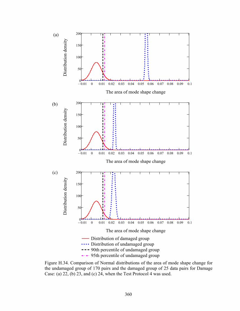
360
Figure H.34. Comparison of Normal distributions of the area of mode shape change forthe undamaged group of 170 pairs and the damaged group of 25 data pairs for DamageCase: (a) 22, (b) 23, and (c) 24, when the Test Protocol 4 was used.
(a)
(b)
(c)
0.01 0 0.01 0.02 0.03 0.04 0.05 0.06 0.07 0.08 0.09 0.10
50
100
150
200
The area of mode shape change
Dis
trib
utio
n de
nsit
y
0.01 0 0.01 0.02 0.03 0.04 0.05 0.06 0.07 0.08 0.09 0.10
50
100
150
200
The area of mode shape change
Dis
trib
utio
n de
nsit
y
0.01 0 0.01 0.02 0.03 0.04 0.05 0.06 0.07 0.08 0.09 0.10
50
100
150
200
Distribution of damaged groupDistribution of undamaged group90th percentile of undamaged group95th percentile of undamaged group
The area of mode shape change
Dis
trib
utio
n de
nsit
y
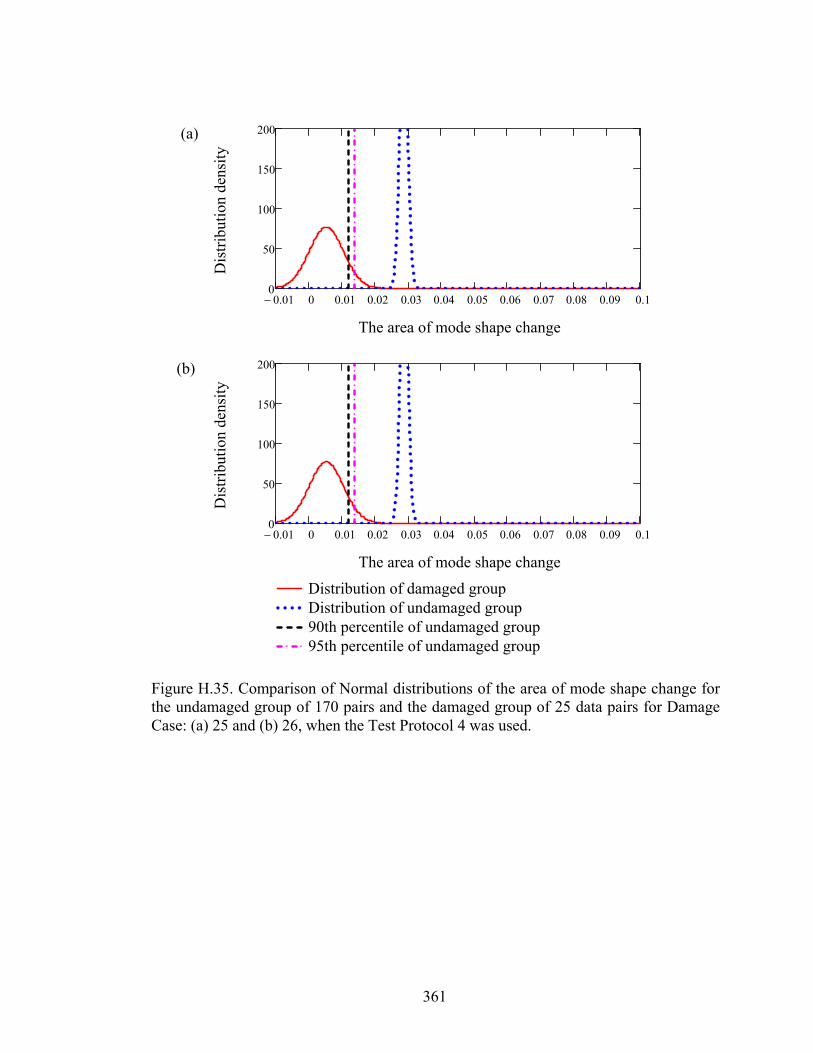
361
Figure H.35. Comparison of Normal distributions of the area of mode shape change forthe undamaged group of 170 pairs and the damaged group of 25 data pairs for DamageCase: (a) 25 and (b) 26, when the Test Protocol 4 was used.
(a)
(b)
0.01 0 0.01 0.02 0.03 0.04 0.05 0.06 0.07 0.08 0.09 0.10
50
100
150
200
The area of mode shape change
Dis
trib
utio
n de
nsit
y
0.01 0 0.01 0.02 0.03 0.04 0.05 0.06 0.07 0.08 0.09 0.10
50
100
150
200
Distribution of damaged groupDistribution of undamaged group90th percentile of undamaged group95th percentile of undamaged group
The area of mode shape change
Dis
trib
utio
n de
nsit
y

362
Table H.40. The probability that there was no change in condition using the assumed Normal distributions (i.e., the probability that the Δ value obtained when there was a change in the condition did not exceed those that obtained when there was no change in condition), for Damage Cases 4 to 9 using all 28 Test Protocols.
Test Protocol
Damage Case
Case 4 Case 5 Case 6 Case 7 Case 8 Case 9 1 0.000% 0.000% 0.000% 0.000% 0.000% 0.000% 2 0.000% 0.000% 0.000% 0.000% 0.000% 0.000% 3 0.000% 0.000% 0.000% 0.000% 0.000% 0.000% 4 10.555% 2.201% 0.252% 4.221% 0.308% 0.287% 5 0.000% 0.942% 0.019% 27.568% 0.001% 1.526% 6 4.310% 31.300% 45.539% 37.756% 30.230% 48.516% 7 32.955% 54.013% 51.868% 51.848% 52.266% 34.480% 8 59.710% 61.961% 62.422% 52.400% 41.114% 39.749% 9 0.818% 0.000% 0.000% 0.000% 0.000% 0.000% 10 0.000% 0.000% 0.000% 0.000% 0.000% 0.000% 11 0.000% 0.000% 0.000% 0.000% 0.000% 0.000% 12 0.000% 0.000% 0.000% 0.000% 0.000% 0.000% 13 56.485% 60.995% 61.519% 60.864% 58.543% 59.378% 14 73.429% 80.325% 59.350% 57.806% 53.954% 62.641% 15 75.329% 82.474% 69.273% 53.833% 59.627% 71.192% 16 74.891% 81.983% 75.312% 54.866% 56.258% 78.444% 17 5.340% 0.000% 0.000% 0.000% 0.000% 0.000% 18 0.000% 0.018% 0.001% 0.000% 5.650% 1.735% 19 0.000% 0.185% 0.085% 0.000% 29.472% 14.048% 20 0.251% 4.872% 0.912% 0.000% 50.494% 36.017% 21 0.000% 3.044% 17.970% 0.000% 14.795% 6.068% 22 3.587% 1.399% 4.629% 8.370% 24.246% 18.136% 23 6.053% 2.565% 8.332% 8.682% 28.424% 18.405% 24 22.432% 7.766% 10.663% 8.019% 31.407% 18.704% 25 0.000% 5.329% 5.261% 0.368% 0.003% 0.036% 26 0.020% 26.180% 42.211% 49.644% 7.113% 32.228% 27 5.905% 18.622% 35.610% 49.974% 8.736% 33.403% 28 24.617% 12.234% 42.786% 58.350% 15.760% 41.053%

363
Table H.41. The probability that there was no change in condition using the assumed Normal distributions (i.e., the probability that the Δ value obtained when there was a change in the condition did not exceed those that obtained when there was no change in condition), for Damage Cases 10 to 15 using all 28 Test Protocols.
Test Protocol
Damage Case
Case 10 Case 11 Case 12 Case 13 Case 14 Case 15 1 0.000% 0.000% 0.000% 0.000% 0.000% 0.000% 2 0.000% 0.000% 0.000% 0.000% 0.002% 0.000% 3 0.000% 0.000% 0.000% 0.000% 0.000% 0.000% 4 0.000% 0.000% 0.000% 2.161% 22.414% 13.883% 5 13.540% 14.797% 14.785% 30.002% 16.348% 28.483% 6 14.579% 30.965% 52.760% 28.864% 41.349% 33.375% 7 15.372% 30.068% 38.004% 30.191% 47.747% 57.679% 8 29.943% 28.377% 42.037% 42.331% 36.438% 48.751% 9 12.746% 35.969% 0.000% 0.000% 5.724% 20.601% 10 0.000% 49.879% 0.000% 0.000% 8.100% 0.000% 11 40.987% 63.141% 0.000% 0.000% 9.348% 0.000% 12 48.592% 60.374% 0.000% 0.000% 10.704% 0.000% 13 54.773% 48.966% 48.426% 42.874% 36.693% 32.919% 14 69.569% 40.072% 32.358% 22.042% 18.889% 13.446% 15 63.944% 37.367% 34.813% 24.886% 20.706% 9.490% 16 55.526% 36.739% 28.276% 29.766% 25.200% 17.713% 17 4.653% 37.327% 0.000% 0.000% 24.926% 23.250% 18 0.001% 52.695% 0.607% 9.178% 19.329% 5.078% 19 15.880% 44.056% 0.511% 17.926% 22.824% 7.842% 20 27.645% 55.553% 1.305% 14.540% 14.660% 16.706% 21 12.281% 35.385% 59.205% 60.827% 61.354% 57.318% 22 8.406% 58.772% 20.762% 59.852% 48.455% 56.504% 23 13.607% 60.925% 23.394% 64.536% 50.706% 54.233% 24 11.683% 60.885% 38.220% 67.579% 59.318% 54.679% 25 0.002% 21.562% 0.725% 4.527% 34.551% 5.019% 26 0.018% 68.693% 41.414% 34.264% 21.751% 4.911% 27 27.751% 52.118% 56.248% 52.431% 26.744% 5.964% 28 33.374% 44.587% 46.708% 39.905% 24.640% 13.131%
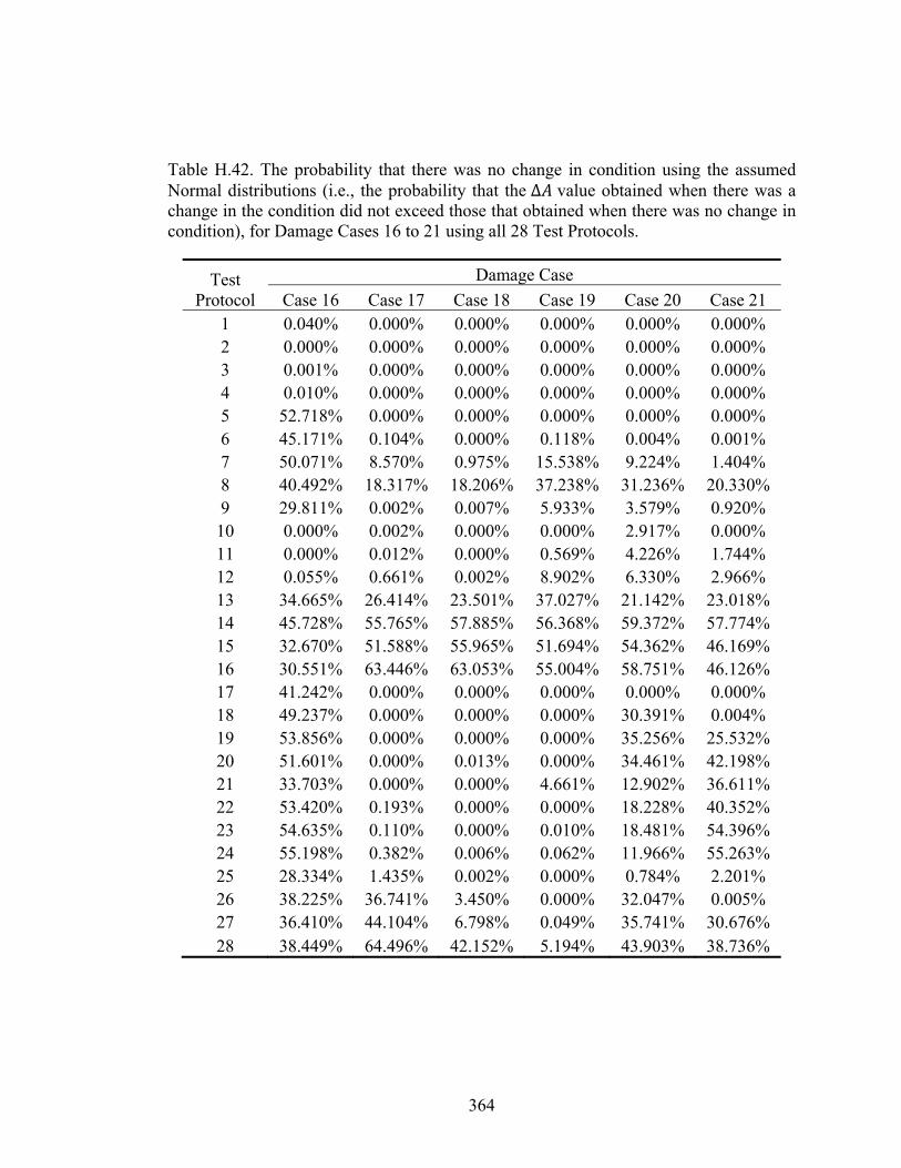
364
Table H.42. The probability that there was no change in condition using the assumed Normal distributions (i.e., the probability that the Δ value obtained when there was a change in the condition did not exceed those that obtained when there was no change in condition), for Damage Cases 16 to 21 using all 28 Test Protocols.
Test Protocol
Damage Case
Case 16 Case 17 Case 18 Case 19 Case 20 Case 21 1 0.040% 0.000% 0.000% 0.000% 0.000% 0.000% 2 0.000% 0.000% 0.000% 0.000% 0.000% 0.000% 3 0.001% 0.000% 0.000% 0.000% 0.000% 0.000% 4 0.010% 0.000% 0.000% 0.000% 0.000% 0.000% 5 52.718% 0.000% 0.000% 0.000% 0.000% 0.000% 6 45.171% 0.104% 0.000% 0.118% 0.004% 0.001% 7 50.071% 8.570% 0.975% 15.538% 9.224% 1.404% 8 40.492% 18.317% 18.206% 37.238% 31.236% 20.330% 9 29.811% 0.002% 0.007% 5.933% 3.579% 0.920% 10 0.000% 0.002% 0.000% 0.000% 2.917% 0.000% 11 0.000% 0.012% 0.000% 0.569% 4.226% 1.744% 12 0.055% 0.661% 0.002% 8.902% 6.330% 2.966% 13 34.665% 26.414% 23.501% 37.027% 21.142% 23.018% 14 45.728% 55.765% 57.885% 56.368% 59.372% 57.774% 15 32.670% 51.588% 55.965% 51.694% 54.362% 46.169% 16 30.551% 63.446% 63.053% 55.004% 58.751% 46.126% 17 41.242% 0.000% 0.000% 0.000% 0.000% 0.000% 18 49.237% 0.000% 0.000% 0.000% 30.391% 0.004% 19 53.856% 0.000% 0.000% 0.000% 35.256% 25.532% 20 51.601% 0.000% 0.013% 0.000% 34.461% 42.198% 21 33.703% 0.000% 0.000% 4.661% 12.902% 36.611% 22 53.420% 0.193% 0.000% 0.000% 18.228% 40.352% 23 54.635% 0.110% 0.000% 0.010% 18.481% 54.396% 24 55.198% 0.382% 0.006% 0.062% 11.966% 55.263% 25 28.334% 1.435% 0.002% 0.000% 0.784% 2.201% 26 38.225% 36.741% 3.450% 0.000% 32.047% 0.005% 27 36.410% 44.104% 6.798% 0.049% 35.741% 30.676% 28 38.449% 64.496% 42.152% 5.194% 43.903% 38.736%
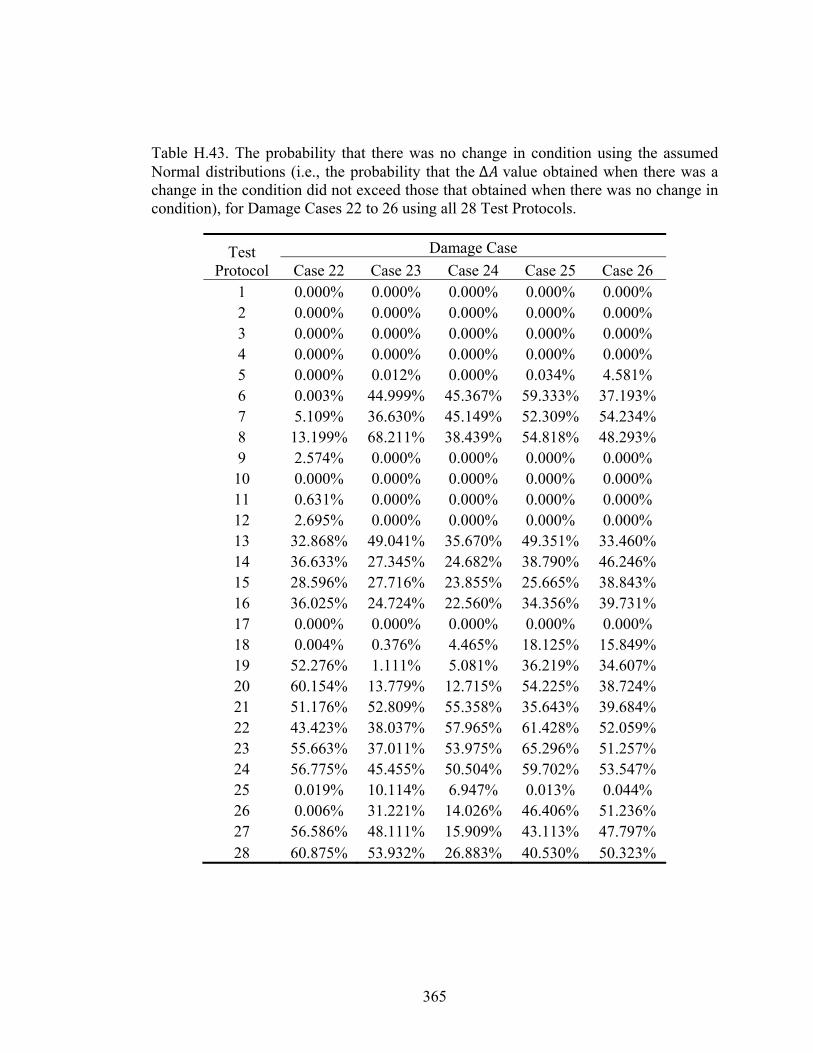
365
Table H.43. The probability that there was no change in condition using the assumed Normal distributions (i.e., the probability that the Δ value obtained when there was a change in the condition did not exceed those that obtained when there was no change in condition), for Damage Cases 22 to 26 using all 28 Test Protocols.
Test Protocol
Damage Case
Case 22 Case 23 Case 24 Case 25 Case 26 1 0.000% 0.000% 0.000% 0.000% 0.000% 2 0.000% 0.000% 0.000% 0.000% 0.000% 3 0.000% 0.000% 0.000% 0.000% 0.000% 4 0.000% 0.000% 0.000% 0.000% 0.000% 5 0.000% 0.012% 0.000% 0.034% 4.581% 6 0.003% 44.999% 45.367% 59.333% 37.193% 7 5.109% 36.630% 45.149% 52.309% 54.234% 8 13.199% 68.211% 38.439% 54.818% 48.293% 9 2.574% 0.000% 0.000% 0.000% 0.000% 10 0.000% 0.000% 0.000% 0.000% 0.000% 11 0.631% 0.000% 0.000% 0.000% 0.000% 12 2.695% 0.000% 0.000% 0.000% 0.000% 13 32.868% 49.041% 35.670% 49.351% 33.460% 14 36.633% 27.345% 24.682% 38.790% 46.246% 15 28.596% 27.716% 23.855% 25.665% 38.843% 16 36.025% 24.724% 22.560% 34.356% 39.731% 17 0.000% 0.000% 0.000% 0.000% 0.000% 18 0.004% 0.376% 4.465% 18.125% 15.849% 19 52.276% 1.111% 5.081% 36.219% 34.607% 20 60.154% 13.779% 12.715% 54.225% 38.724% 21 51.176% 52.809% 55.358% 35.643% 39.684% 22 43.423% 38.037% 57.965% 61.428% 52.059% 23 55.663% 37.011% 53.975% 65.296% 51.257% 24 56.775% 45.455% 50.504% 59.702% 53.547% 25 0.019% 10.114% 6.947% 0.013% 0.044% 26 0.006% 31.221% 14.026% 46.406% 51.236% 27 56.586% 48.111% 15.909% 43.113% 47.797% 28 60.875% 53.932% 26.883% 40.530% 50.323%

366
Table H.44. The probability that there was no change in condition using the assumed Log-Normal distributions (i.e., the probability that the Δ value obtained when there was a change in the condition did not exceed those that obtained when there was no change in condition), for Damage Cases 4 to 9 using all 28 Test Protocols.
Test Protocol
Damage Case
Case 4 Case 5 Case 6 Case 7 Case 8 Case 9 1 0.468% 0.120% 0.043% 0.175% 0.064% 0.064% 2 0.000% 0.000% 0.000% 0.000% 0.000% 0.000% 3 0.000% 0.000% 0.000% 0.000% 0.000% 0.000% 4 3.297% 0.312% 0.020% 0.745% 0.021% 0.020% 5 0.001% 1.829% 0.803% 24.769% 0.813% 2.174% 6 6.126% 30.897% 44.020% 37.888% 29.220% 47.043% 7 32.413% 51.741% 50.832% 50.505% 51.555% 33.934% 8 57.728% 60.266% 61.808% 50.837% 42.378% 40.578% 9 6.548% 0.310% 0.226% 0.272% 0.300% 0.311% 10 0.007% 0.000% 0.000% 0.000% 0.000% 0.000% 11 0.014% 0.000% 0.000% 0.000% 0.000% 0.000% 12 0.329% 0.000% 0.000% 0.000% 0.000% 0.000% 13 47.697% 61.242% 62.606% 61.812% 55.837% 58.263% 14 72.620% 84.009% 55.494% 54.771% 48.515% 57.291% 15 74.429% 86.051% 66.755% 50.835% 52.703% 67.763% 16 72.582% 82.878% 74.043% 51.669% 50.820% 77.457% 17 5.415% 0.000% 0.000% 0.000% 0.033% 0.021% 18 0.001% 0.078% 0.013% 0.000% 5.424% 2.108% 19 0.013% 0.548% 0.253% 0.000% 24.316% 12.612% 20 1.138% 5.213% 1.922% 0.005% 46.803% 32.432% 21 1.603% 8.254% 17.156% 0.357% 15.480% 10.047% 22 3.881% 2.167% 4.155% 6.375% 17.358% 13.328% 23 4.646% 2.589% 5.767% 6.035% 21.548% 12.392% 24 16.720% 7.248% 9.176% 7.612% 25.456% 14.601% 25 0.000% 6.316% 6.356% 0.458% 0.026% 0.246% 26 0.922% 21.016% 35.560% 42.846% 4.900% 29.557% 27 5.834% 14.632% 30.605% 42.207% 6.318% 30.437% 28 20.536% 11.358% 39.058% 54.099% 14.092% 38.523%
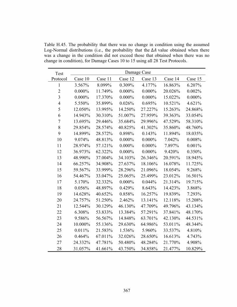
367
Table H.45. The probability that there was no change in condition using the assumed Log-Normal distributions (i.e., the probability that the Δ value obtained when there was a change in the condition did not exceed those that obtained when there was no change in condition), for Damage Cases 10 to 15 using all 28 Test Protocols.
Test Protocol
Damage Case
Case 10 Case 11 Case 12 Case 13 Case 14 Case 15 1 3.567% 8.099% 0.309% 4.177% 16.863% 6.207% 2 0.000% 11.749% 0.000% 0.000% 20.026% 0.002% 3 0.000% 17.370% 0.000% 0.000% 15.022% 0.000% 4 5.550% 35.899% 0.026% 0.695% 10.521% 4.621% 5 12.050% 13.995% 14.250% 27.227% 15.263% 24.868% 6 14.943% 30.310% 51.007% 27.959% 39.363% 33.054% 7 13.695% 29.446% 35.684% 29.996% 47.529% 58.310% 8 29.854% 28.574% 40.825% 41.302% 35.860% 48.760% 9 14.899% 28.572% 0.898% 0.143% 11.894% 18.035% 10 9.074% 48.813% 0.000% 0.000% 7.042% 0.008% 11 28.974% 57.121% 0.000% 0.000% 7.897% 0.001% 12 36.973% 62.322% 0.000% 0.000% 9.420% 0.350% 13 48.990% 37.004% 34.103% 26.346% 20.591% 18.945% 14 66.257% 34.908% 27.637% 18.106% 16.078% 11.725% 15 59.567% 33.999% 28.296% 21.096% 18.054% 9.268% 16 54.467% 33.047% 25.065% 25.499% 23.012% 16.501% 17 5.170% 32.332% 0.000% 0.044% 21.314% 19.715% 18 0.056% 48.897% 0.429% 8.643% 14.423% 3.868% 19 14.628% 40.652% 0.858% 16.257% 19.839% 7.293% 20 24.757% 51.250% 2.462% 13.141% 12.118% 15.208% 21 12.544% 30.129% 46.130% 47.709% 49.796% 43.134% 22 6.308% 53.833% 13.384% 57.291% 37.841% 48.170% 23 9.586% 56.567% 14.848% 63.701% 42.130% 44.531% 24 10.000% 55.136% 29.630% 64.986% 53.011% 48.344% 25 0.011% 21.583% 1.536% 5.960% 33.537% 4.810% 26 0.464% 67.011% 32.026% 28.650% 16.613% 4.743% 27 24.332% 47.781% 50.480% 48.284% 21.770% 4.908% 28 31.057% 41.661% 43.750% 34.858% 21.477% 10.829%
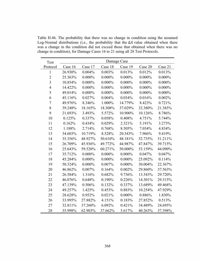
368
Table H.46. The probability that there was no change in condition using the assumed Log-Normal distributions (i.e., the probability that the Δ value obtained when there was a change in the condition did not exceed those that obtained when there was no change in condition), for Damage Cases 16 to 21 using all 28 Test Protocols.
Test Protocol
Damage Case
Case 16 Case 17 Case 18 Case 19 Case 20 Case 21 1 26.930% 0.004% 0.003% 0.013% 0.012% 0.013% 2 25.363% 0.000% 0.000% 0.000% 0.000% 0.000% 3 10.854% 0.000% 0.000% 0.000% 0.000% 0.000% 4 14.422% 0.000% 0.000% 0.000% 0.000% 0.000% 5 49.014% 0.000% 0.000% 0.000% 0.000% 0.000% 6 45.116% 0.027% 0.004% 0.034% 0.016% 0.002% 7 49.976% 8.346% 1.000% 14.779% 8.423% 0.721% 8 39.248% 18.165% 18.308% 37.029% 32.380% 21.385% 9 21.693% 3.493% 5.572% 10.900% 10.126% 8.786% 10 0.125% 0.337% 0.058% 0.408% 4.751% 5.744% 11 0.162% 0.434% 0.029% 2.321% 5.191% 3.273% 12 1.188% 2.714% 0.768% 8.505% 7.034% 4.834% 13 34.603% 10.719% 8.528% 20.543% 7.966% 9.419% 14 35.356% 48.927% 50.610% 48.181% 52.735% 51.211% 15 26.709% 45.936% 49.772% 44.987% 47.847% 39.715% 16 25.643% 59.520% 60.271% 50.000% 53.159% 44.090% 17 35.712% 0.000% 0.000% 0.000% 0.047% 0.047% 18 45.284% 0.000% 0.000% 0.000% 25.092% 0.114% 19 50.324% 0.000% 0.007% 0.000% 30.004% 22.367% 20 46.862% 0.007% 0.164% 0.002% 29.860% 37.563% 21 26.584% 1.316% 0.682% 9.736% 13.543% 29.720% 22 46.076% 0.648% 0.190% 0.226% 14.301% 29.315% 23 47.139% 0.506% 0.132% 0.337% 13.689% 49.468% 24 49.257% 1.425% 0.453% 0.883% 10.254% 47.929% 25 28.628% 0.952% 0.021% 0.000% 0.886% 1.830% 26 33.995% 27.882% 4.151% 0.183% 27.852% 0.513% 27 32.811% 37.260% 6.092% 0.421% 34.489% 24.695% 28 35.998% 62.903% 37.662% 5.617% 40.263% 37.398%
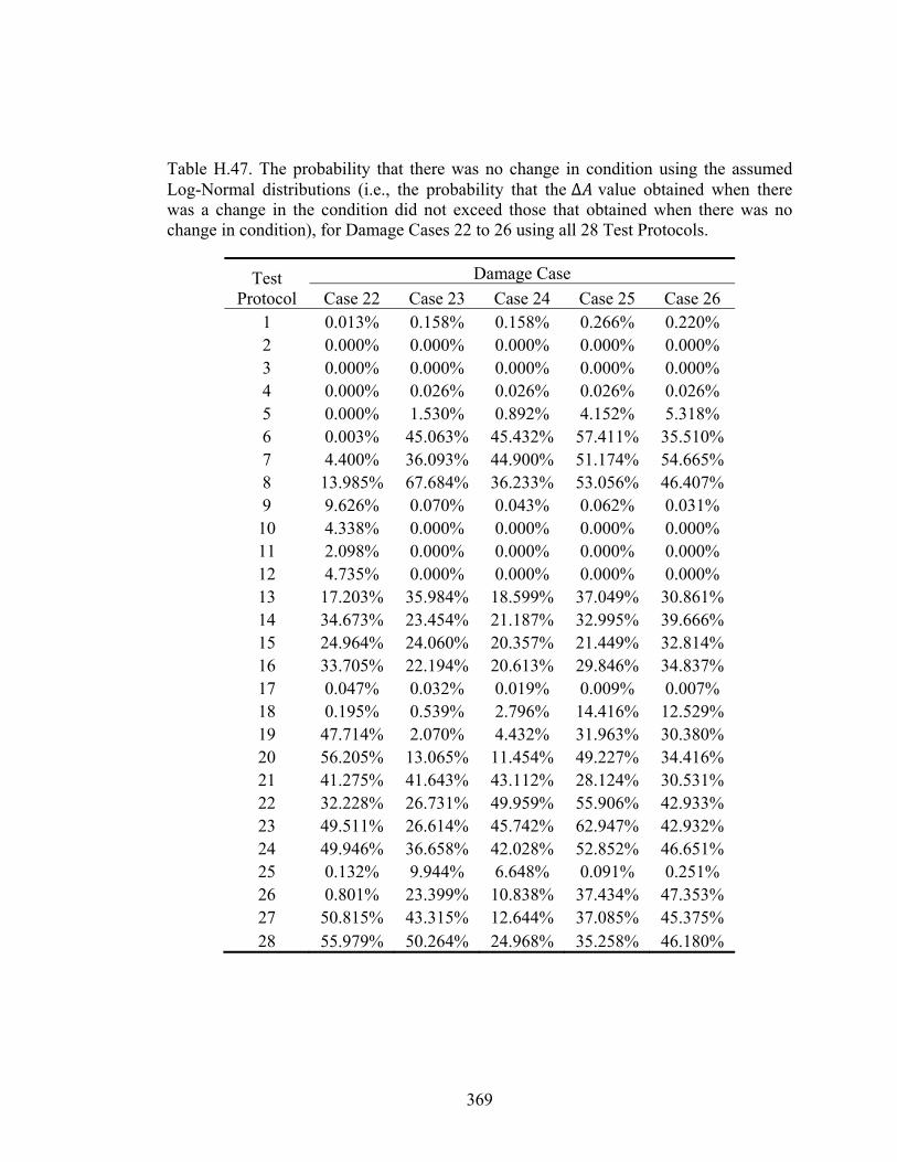
369
Table H.47. The probability that there was no change in condition using the assumed Log-Normal distributions (i.e., the probability that the Δ value obtained when there was a change in the condition did not exceed those that obtained when there was no change in condition), for Damage Cases 22 to 26 using all 28 Test Protocols.
Test Protocol
Damage Case
Case 22 Case 23 Case 24 Case 25 Case 26 1 0.013% 0.158% 0.158% 0.266% 0.220% 2 0.000% 0.000% 0.000% 0.000% 0.000% 3 0.000% 0.000% 0.000% 0.000% 0.000% 4 0.000% 0.026% 0.026% 0.026% 0.026% 5 0.000% 1.530% 0.892% 4.152% 5.318% 6 0.003% 45.063% 45.432% 57.411% 35.510% 7 4.400% 36.093% 44.900% 51.174% 54.665% 8 13.985% 67.684% 36.233% 53.056% 46.407% 9 9.626% 0.070% 0.043% 0.062% 0.031% 10 4.338% 0.000% 0.000% 0.000% 0.000% 11 2.098% 0.000% 0.000% 0.000% 0.000% 12 4.735% 0.000% 0.000% 0.000% 0.000% 13 17.203% 35.984% 18.599% 37.049% 30.861% 14 34.673% 23.454% 21.187% 32.995% 39.666% 15 24.964% 24.060% 20.357% 21.449% 32.814% 16 33.705% 22.194% 20.613% 29.846% 34.837% 17 0.047% 0.032% 0.019% 0.009% 0.007% 18 0.195% 0.539% 2.796% 14.416% 12.529% 19 47.714% 2.070% 4.432% 31.963% 30.380% 20 56.205% 13.065% 11.454% 49.227% 34.416% 21 41.275% 41.643% 43.112% 28.124% 30.531% 22 32.228% 26.731% 49.959% 55.906% 42.933% 23 49.511% 26.614% 45.742% 62.947% 42.932% 24 49.946% 36.658% 42.028% 52.852% 46.651% 25 0.132% 9.944% 6.648% 0.091% 0.251% 26 0.801% 23.399% 10.838% 37.434% 47.353% 27 50.815% 43.315% 12.644% 37.085% 45.375% 28 55.979% 50.264% 24.968% 35.258% 46.180%
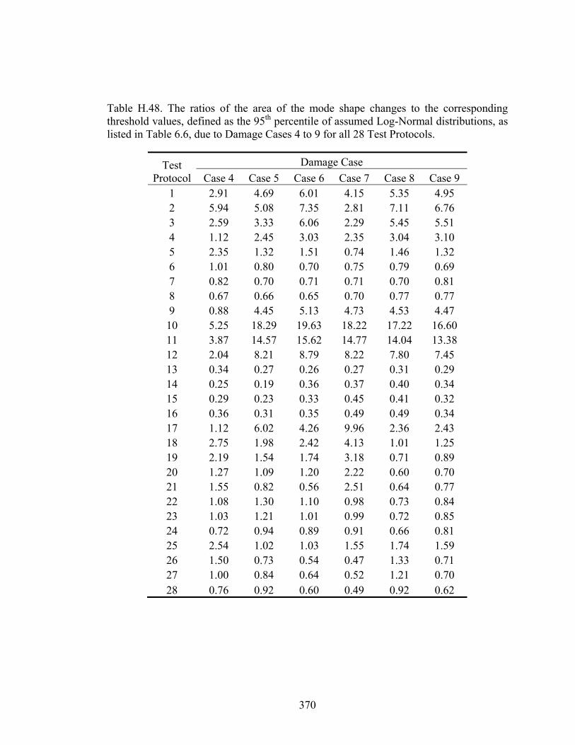
370
Table H.48. The ratios of the area of the mode shape changes to the corresponding threshold values, defined as the 95th percentile of assumed Log-Normal distributions, as listed in Table 6.6, due to Damage Cases 4 to 9 for all 28 Test Protocols.
Test Protocol
Damage Case
Case 4 Case 5 Case 6 Case 7 Case 8 Case 9 1 2.91 4.69 6.01 4.15 5.35 4.95 2 5.94 5.08 7.35 2.81 7.11 6.76 3 2.59 3.33 6.06 2.29 5.45 5.51 4 1.12 2.45 3.03 2.35 3.04 3.10 5 2.35 1.32 1.51 0.74 1.46 1.32 6 1.01 0.80 0.70 0.75 0.79 0.69 7 0.82 0.70 0.71 0.71 0.70 0.81 8 0.67 0.66 0.65 0.70 0.77 0.77 9 0.88 4.45 5.13 4.73 4.53 4.47 10 5.25 18.29 19.63 18.22 17.22 16.60 11 3.87 14.57 15.62 14.77 14.04 13.38 12 2.04 8.21 8.79 8.22 7.80 7.45 13 0.34 0.27 0.26 0.27 0.31 0.29 14 0.25 0.19 0.36 0.37 0.40 0.34 15 0.29 0.23 0.33 0.45 0.41 0.32 16 0.36 0.31 0.35 0.49 0.49 0.34 17 1.12 6.02 4.26 9.96 2.36 2.43 18 2.75 1.98 2.42 4.13 1.01 1.25 19 2.19 1.54 1.74 3.18 0.71 0.89 20 1.27 1.09 1.20 2.22 0.60 0.70 21 1.55 0.82 0.56 2.51 0.64 0.77 22 1.08 1.30 1.10 0.98 0.73 0.84 23 1.03 1.21 1.01 0.99 0.72 0.85 24 0.72 0.94 0.89 0.91 0.66 0.81 25 2.54 1.02 1.03 1.55 1.74 1.59 26 1.50 0.73 0.54 0.47 1.33 0.71 27 1.00 0.84 0.64 0.52 1.21 0.70 28 0.76 0.92 0.60 0.49 0.92 0.62
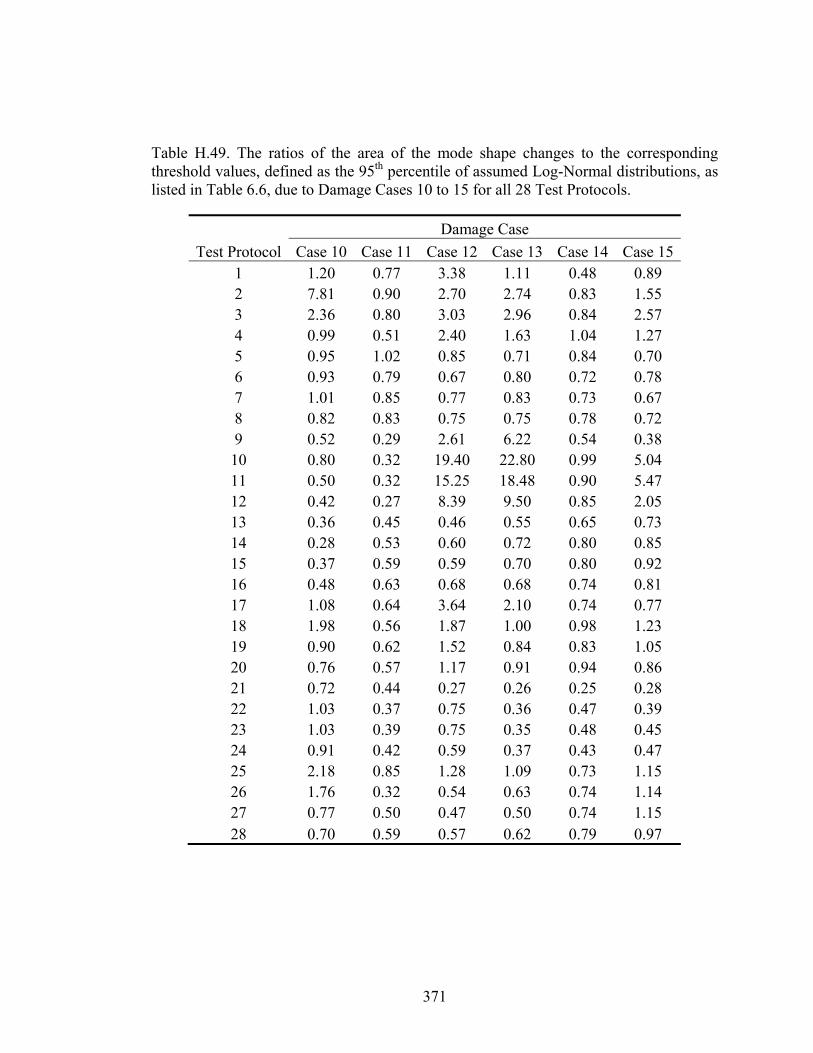
371
Table H.49. The ratios of the area of the mode shape changes to the corresponding threshold values, defined as the 95th percentile of assumed Log-Normal distributions, as listed in Table 6.6, due to Damage Cases 10 to 15 for all 28 Test Protocols.
Test Protocol
Damage Case
Case 10 Case 11 Case 12 Case 13 Case 14 Case 151 1.20 0.77 3.38 1.11 0.48 0.89 2 7.81 0.90 2.70 2.74 0.83 1.55 3 2.36 0.80 3.03 2.96 0.84 2.57 4 0.99 0.51 2.40 1.63 1.04 1.27 5 0.95 1.02 0.85 0.71 0.84 0.70 6 0.93 0.79 0.67 0.80 0.72 0.78 7 1.01 0.85 0.77 0.83 0.73 0.67 8 0.82 0.83 0.75 0.75 0.78 0.72 9 0.52 0.29 2.61 6.22 0.54 0.38 10 0.80 0.32 19.40 22.80 0.99 5.04 11 0.50 0.32 15.25 18.48 0.90 5.47 12 0.42 0.27 8.39 9.50 0.85 2.05 13 0.36 0.45 0.46 0.55 0.65 0.73 14 0.28 0.53 0.60 0.72 0.80 0.85 15 0.37 0.59 0.59 0.70 0.80 0.92 16 0.48 0.63 0.68 0.68 0.74 0.81 17 1.08 0.64 3.64 2.10 0.74 0.77 18 1.98 0.56 1.87 1.00 0.98 1.23 19 0.90 0.62 1.52 0.84 0.83 1.05 20 0.76 0.57 1.17 0.91 0.94 0.86 21 0.72 0.44 0.27 0.26 0.25 0.28 22 1.03 0.37 0.75 0.36 0.47 0.39 23 1.03 0.39 0.75 0.35 0.48 0.45 24 0.91 0.42 0.59 0.37 0.43 0.47 25 2.18 0.85 1.28 1.09 0.73 1.15 26 1.76 0.32 0.54 0.63 0.74 1.14 27 0.77 0.50 0.47 0.50 0.74 1.15 28 0.70 0.59 0.57 0.62 0.79 0.97
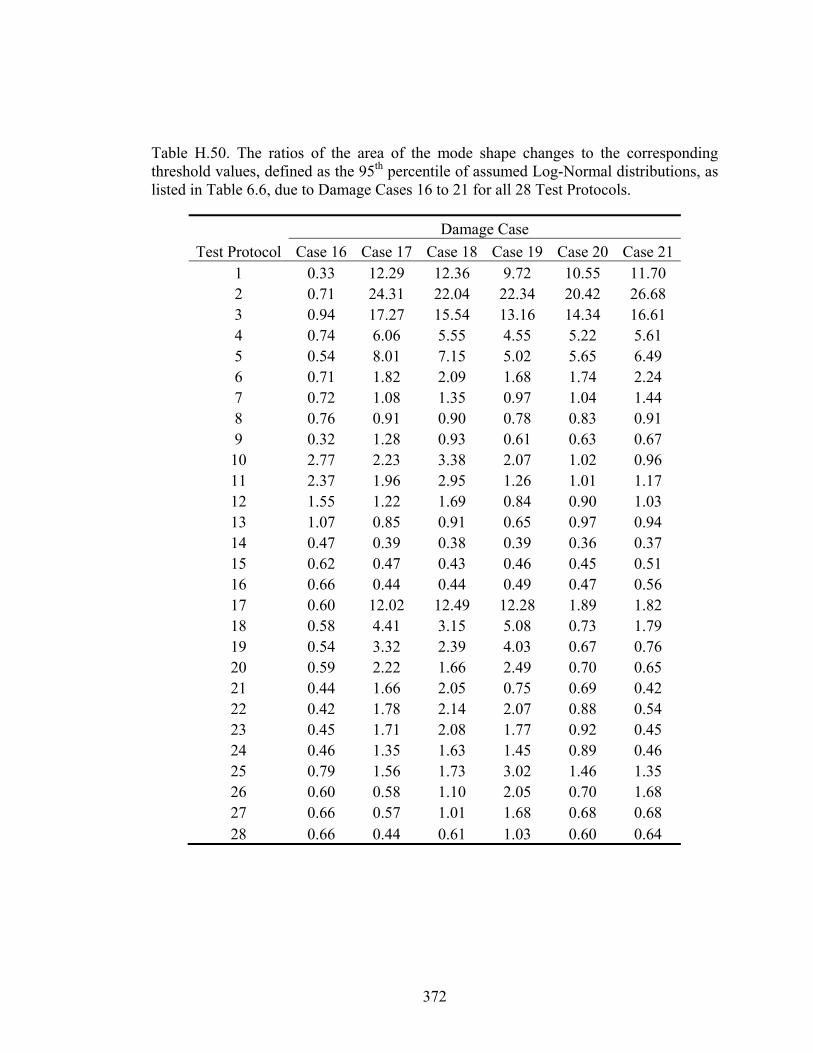
372
Table H.50. The ratios of the area of the mode shape changes to the corresponding threshold values, defined as the 95th percentile of assumed Log-Normal distributions, as listed in Table 6.6, due to Damage Cases 16 to 21 for all 28 Test Protocols.
Test Protocol
Damage Case
Case 16 Case 17 Case 18 Case 19 Case 20 Case 211 0.33 12.29 12.36 9.72 10.55 11.70 2 0.71 24.31 22.04 22.34 20.42 26.68 3 0.94 17.27 15.54 13.16 14.34 16.61 4 0.74 6.06 5.55 4.55 5.22 5.61 5 0.54 8.01 7.15 5.02 5.65 6.49 6 0.71 1.82 2.09 1.68 1.74 2.24 7 0.72 1.08 1.35 0.97 1.04 1.44 8 0.76 0.91 0.90 0.78 0.83 0.91 9 0.32 1.28 0.93 0.61 0.63 0.67 10 2.77 2.23 3.38 2.07 1.02 0.96 11 2.37 1.96 2.95 1.26 1.01 1.17 12 1.55 1.22 1.69 0.84 0.90 1.03 13 1.07 0.85 0.91 0.65 0.97 0.94 14 0.47 0.39 0.38 0.39 0.36 0.37 15 0.62 0.47 0.43 0.46 0.45 0.51 16 0.66 0.44 0.44 0.49 0.47 0.56 17 0.60 12.02 12.49 12.28 1.89 1.82 18 0.58 4.41 3.15 5.08 0.73 1.79 19 0.54 3.32 2.39 4.03 0.67 0.76 20 0.59 2.22 1.66 2.49 0.70 0.65 21 0.44 1.66 2.05 0.75 0.69 0.42 22 0.42 1.78 2.14 2.07 0.88 0.54 23 0.45 1.71 2.08 1.77 0.92 0.45 24 0.46 1.35 1.63 1.45 0.89 0.46 25 0.79 1.56 1.73 3.02 1.46 1.35 26 0.60 0.58 1.10 2.05 0.70 1.68 27 0.66 0.57 1.01 1.68 0.68 0.68 28 0.66 0.44 0.61 1.03 0.60 0.64

373
Table H.51. The ratios of the area of the mode shape changes to the corresponding threshold values, defined as the 95th percentile of assumed Log-Normal distributions, as listed in Table 6.6, due to Damage Cases 22 to 26 for all 28 Test Protocols.
Test Protocol
Damage Case
Case 22 Case 23 Case 24 Case 25 Case 26 1 11.37 4.27 4.43 3.55 3.82 2 26.41 4.66 4.41 4.44 4.11 3 16.19 5.49 5.56 3.66 3.70 4 5.45 2.31 2.23 2.77 2.78 5 5.82 1.33 1.41 1.09 1.10 6 2.22 0.71 0.71 0.63 0.75 7 1.19 0.80 0.74 0.70 0.69 8 0.95 0.62 0.76 0.69 0.72 9 0.64 7.81 8.27 8.08 8.38 10 1.05 35.53 35.34 37.02 36.13 11 1.33 27.13 26.98 29.15 28.39 12 1.03 15.37 15.43 15.74 15.82 13 0.73 0.45 0.67 0.45 1.12 14 0.57 0.69 0.72 0.54 0.47 15 0.67 0.70 0.73 0.69 0.57 16 0.64 0.72 0.78 0.64 0.60 17 2.14 2.34 2.45 2.52 2.55 18 1.64 1.59 1.44 0.85 0.87 19 0.56 1.25 1.18 0.67 0.68 20 0.54 0.92 0.95 0.57 0.67 21 0.32 0.31 0.29 0.42 0.39 22 0.51 0.56 0.38 0.35 0.43 23 0.44 0.61 0.45 0.35 0.48 24 0.45 0.54 0.50 0.43 0.47 25 1.74 1.00 1.09 1.78 1.60 26 1.54 0.64 0.87 0.50 0.46 27 0.47 0.53 0.89 0.57 0.54 28 0.48 0.52 0.76 0.62 0.55
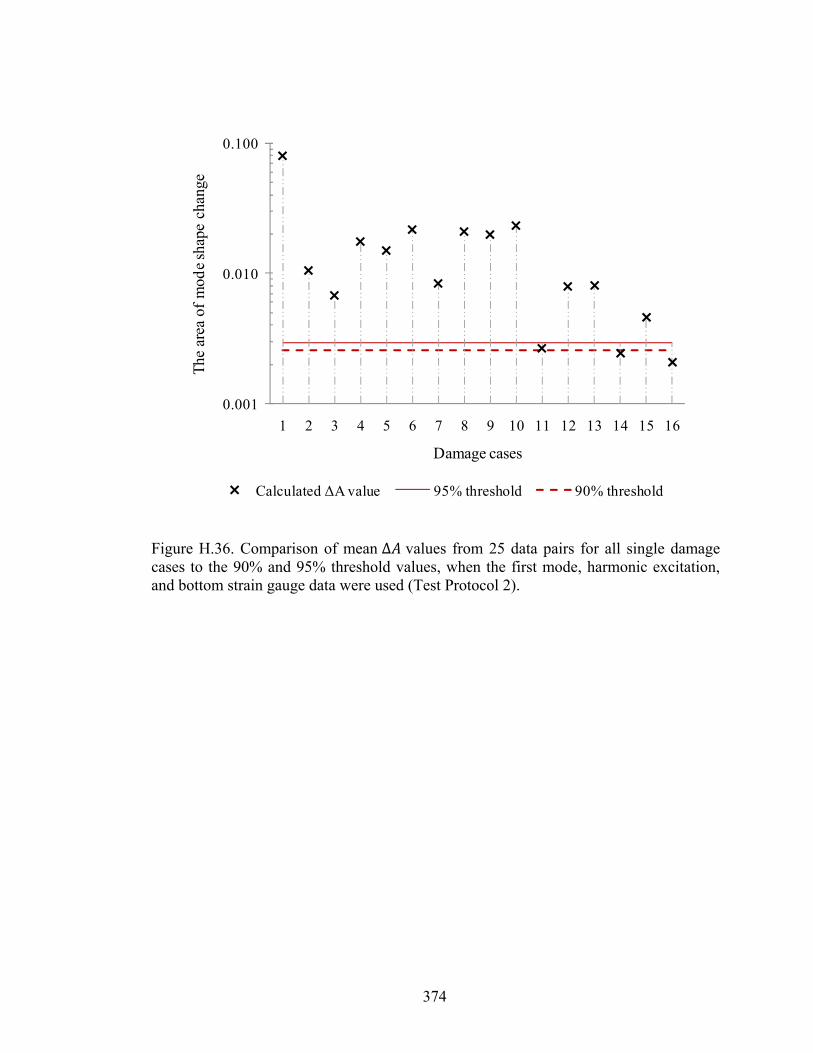
374
Figure H.36. Comparison of mean Δ values from 25 data pairs for all single damagecases to the 90% and 95% threshold values, when the first mode, harmonic excitation,and bottom strain gauge data were used (Test Protocol 2).
0.001
0.010
0.100
1 2 3 4 5 6 7 8 9 10 11 12 13 14 15 16
The
are
a of
mod
e sh
ape
chan
ge
Damage cases
Calculated ΔA value 95% threshold 90% threshold
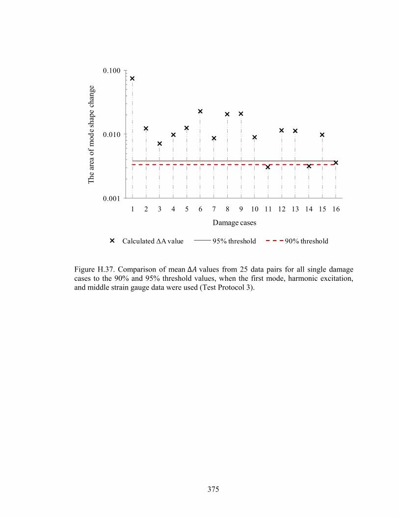
375
Figure H.37. Comparison of mean Δ values from 25 data pairs for all single damagecases to the 90% and 95% threshold values, when the first mode, harmonic excitation,and middle strain gauge data were used (Test Protocol 3).
0.001
0.010
0.100
1 2 3 4 5 6 7 8 9 10 11 12 13 14 15 16
The
are
a of
mod
e sh
ape
chan
ge
Damage cases
Calculated ΔA value 95% threshold 90% threshold

376
Figure H.38. Comparison of mean Δ values from 25 data pairs for all single damagecases to the 90% and 95% threshold values, when the first mode, harmonic excitation,and top strain gauge data were used (Test Protocol 4).
0.001
0.010
0.100
1 2 3 4 5 6 7 8 9 10 11 12 13 14 15 16
The
are
a of
mod
e sh
ape
chan
ge
Damage cases
Calculated ΔA value 95% threshold 90% threshold
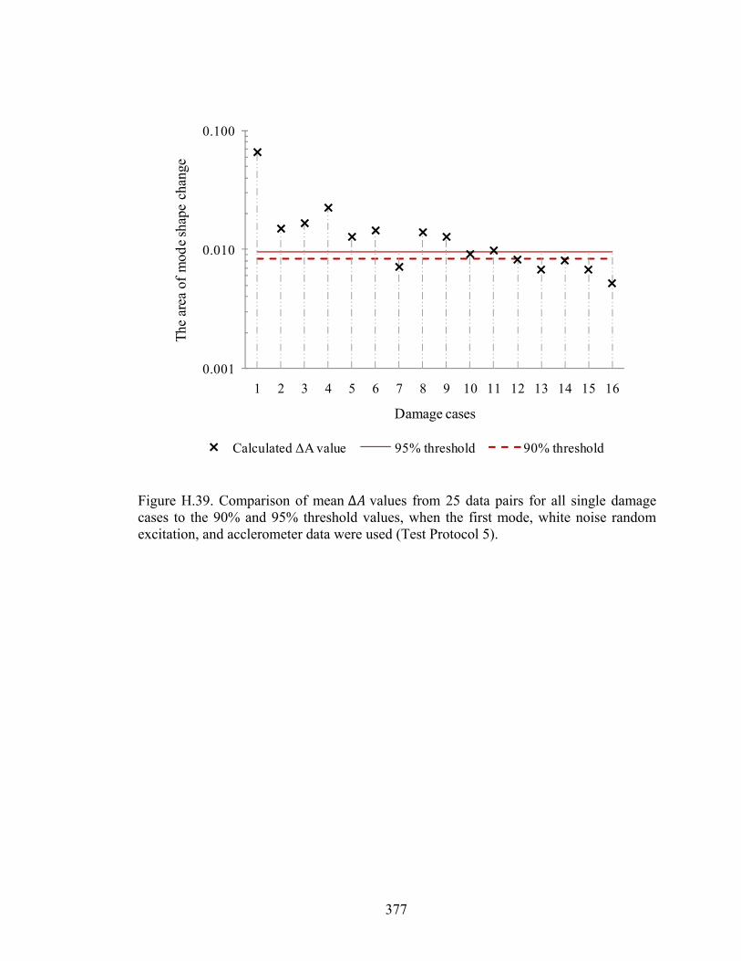
377
Figure H.39. Comparison of mean Δ values from 25 data pairs for all single damagecases to the 90% and 95% threshold values, when the first mode, white noise randomexcitation, and acclerometer data were used (Test Protocol 5).
0.001
0.010
0.100
1 2 3 4 5 6 7 8 9 10 11 12 13 14 15 16
The
are
a of
mod
e sh
ape
chan
ge
Damage cases
Calculated ΔA value 95% threshold 90% threshold
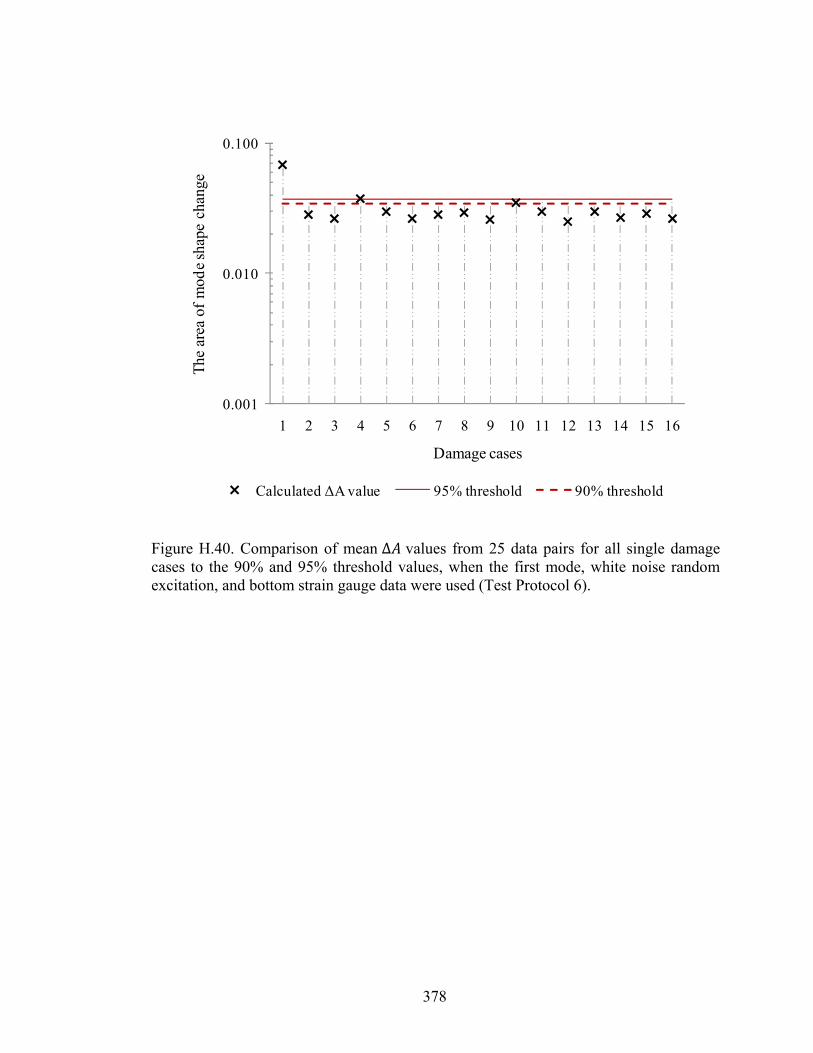
378
Figure H.40. Comparison of mean Δ values from 25 data pairs for all single damagecases to the 90% and 95% threshold values, when the first mode, white noise randomexcitation, and bottom strain gauge data were used (Test Protocol 6).
0.001
0.010
0.100
1 2 3 4 5 6 7 8 9 10 11 12 13 14 15 16
The
are
a of
mod
e sh
ape
chan
ge
Damage cases
Calculated ΔA value 95% threshold 90% threshold
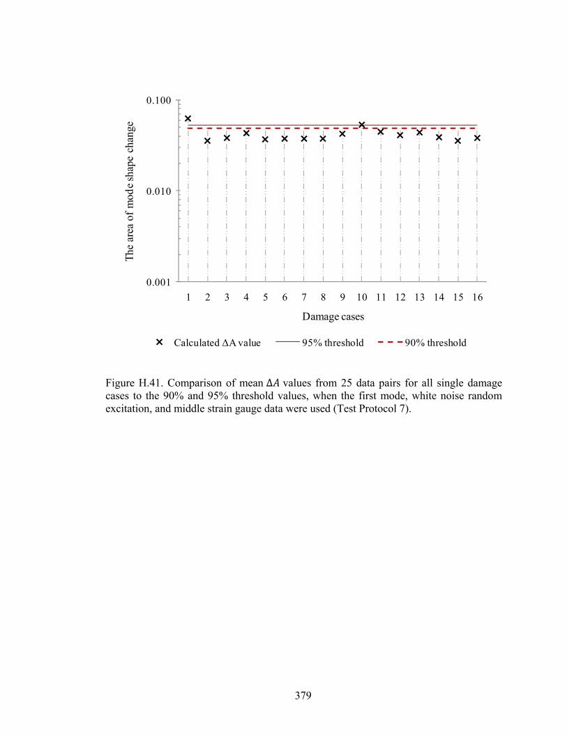
379
Figure H.41. Comparison of mean Δ values from 25 data pairs for all single damagecases to the 90% and 95% threshold values, when the first mode, white noise randomexcitation, and middle strain gauge data were used (Test Protocol 7).
0.001
0.010
0.100
1 2 3 4 5 6 7 8 9 10 11 12 13 14 15 16
The
are
a of
mod
e sh
ape
chan
ge
Damage cases
Calculated ΔA value 95% threshold 90% threshold

380
Figure H.42. Comparison of mean Δ values from 25 data pairs for all single damagecases to the 90% and 95% threshold values, when the first mode, white noise randomexcitation, and top strain gauge data were used (Test Protocol 8).
0.001
0.010
0.100
1 2 3 4 5 6 7 8 9 10 11 12 13 14 15 16
The
are
a of
mod
e sh
ape
chan
ge
Damage cases
Calculated ΔA value 95% threshold 90% threshold
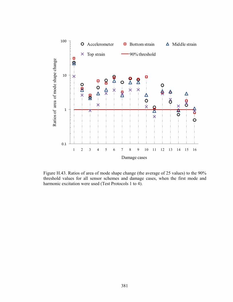
381
Figure H.43. Ratios of area of mode shape change (the average of 25 values) to the 90%threshold values for all sensor schemes and damage cases, when the first mode andharmonic excitation were used (Test Protocols 1 to 4).
0.1
1
10
100
1 2 3 4 5 6 7 8 9 10 11 12 13 14 15 16
Rat
ios
of a
rea
of m
ode
shap
e ch
ange
Damage cases
Accelerometer Bottom strain Middle strain
Top strain 90% threshold

382
Figure H.44. Ratios of area of mode shape change (the average of 25 values) to the 90%threshold values for all sensor schemes and damage cases, when the first mode andwhite noise random excitation were used (Test Protocols 5 to 8).
0.1
1
10
100
1 2 3 4 5 6 7 8 9 10 11 12 13 14 15 16
Rat
ios
of a
rea
of m
ode
shap
e ch
ange
Damage cases
Accelerometer Bottom strain Middle strain
Top strain 90% threshold
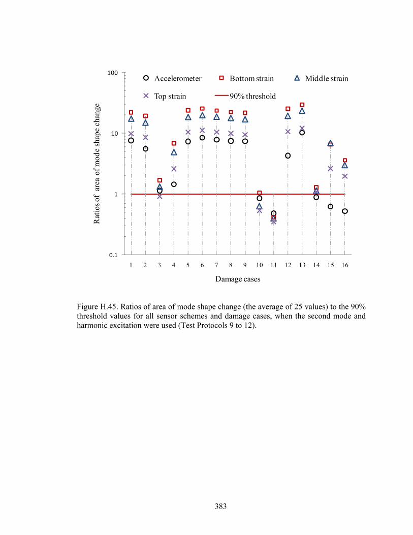
383
Figure H.45. Ratios of area of mode shape change (the average of 25 values) to the 90%threshold values for all sensor schemes and damage cases, when the second mode andharmonic excitation were used (Test Protocols 9 to 12).
0.1
1
10
100
1 2 3 4 5 6 7 8 9 10 11 12 13 14 15 16
Rat
ios
of a
rea
of m
ode
shap
e ch
ange
Damage cases
Accelerometer Bottom strain Middle strain
Top strain 90% threshold
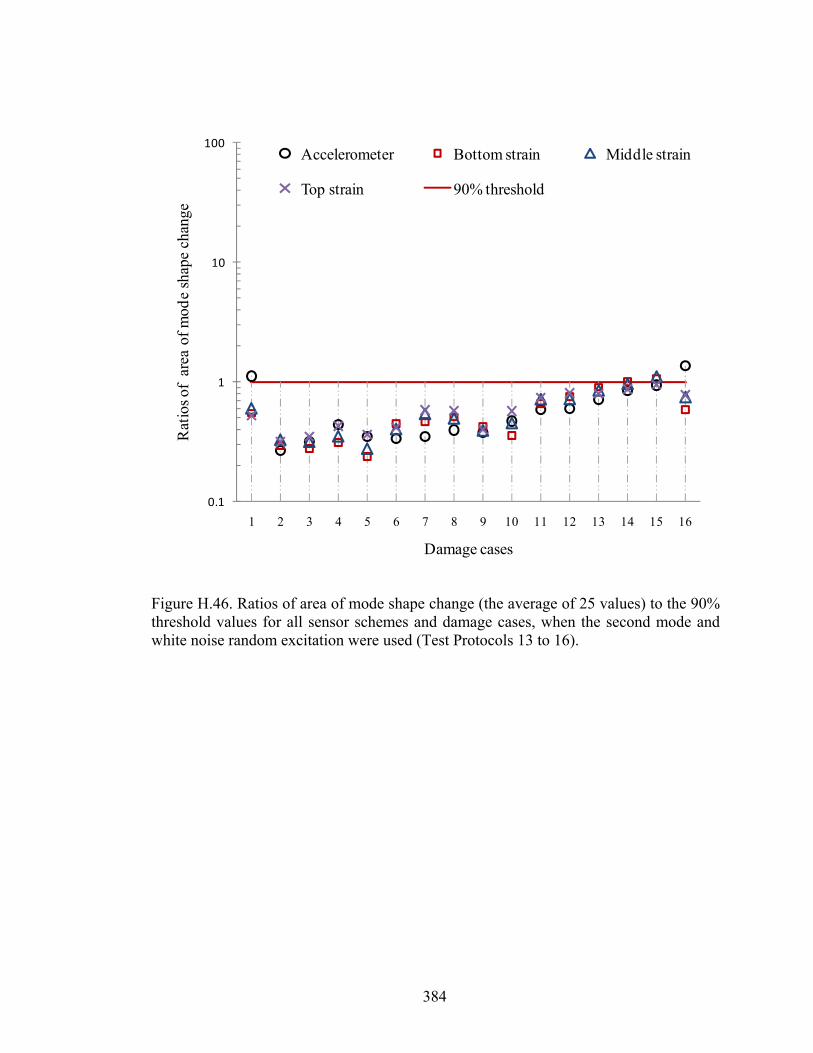
384
Figure H.46. Ratios of area of mode shape change (the average of 25 values) to the 90%threshold values for all sensor schemes and damage cases, when the second mode andwhite noise random excitation were used (Test Protocols 13 to 16).
0.1
1
10
100
1 2 3 4 5 6 7 8 9 10 11 12 13 14 15 16
Rat
ios
of a
rea
of m
ode
shap
e ch
ange
Damage cases
Accelerometer Bottom strain Middle strain
Top strain 90% threshold
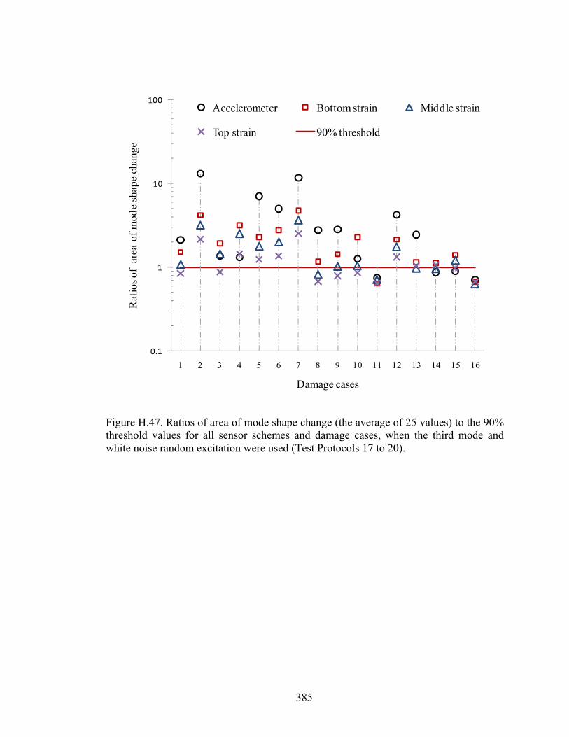
385
Figure H.47. Ratios of area of mode shape change (the average of 25 values) to the 90%threshold values for all sensor schemes and damage cases, when the third mode andwhite noise random excitation were used (Test Protocols 17 to 20).
0.1
1
10
100
1 2 3 4 5 6 7 8 9 10 11 12 13 14 15 16
Rat
ios
of a
rea
of m
ode
shap
e ch
ange
Damage cases
Accelerometer Bottom strain Middle strain
Top strain 90% threshold

386
Figure H.48. Ratios of area of mode shape change (the average of 25 values) to the 90%threshold values for all sensor schemes and damage cases, when the fourth mode andwhite noise random excitation were used (Test Protocols 21 to 24).
0.1
1
10
100
1 2 3 4 5 6 7 8 9 10 11 12 13 14 15 16
Rat
ios
of a
rea
of m
ode
shap
e ch
ange
Damage cases
Accelerometer Bottom strain Middle strain
Top strain 90% threshold

387
Figure H.49. Ratios of area of mode shape change (the average of 25 values) to the 90%threshold values for all sensor schemes and damage cases, when the fifth mode andwhite noise random excitation were used (Test Protocols 25 to 28).
0.1
1
10
100
1 2 3 4 5 6 7 8 9 10 11 12 13 14 15 16
Rat
ios
of a
rea
of m
ode
shap
e ch
ange
Damage cases
Accelerometer Bottom strain Middle strain
Top strain 90% threshold
388
APPENDIX I. DETECTION OF DAMAGE CASE 1 USING
COMMONLY AVAILABLE VBDD INDICATORS
BASED ON THE FIRST MODE SHAPE
This appendix present additional information for Section 6.3, providing damage
localization of Damage Case 1 using commonly available VBDD indicators based on
the first mode shape. The damage indicators used in this Appendix included change in
mode shape method, damage index method, and change in mode shape curvature
method.
Figures I.1 to I.3 present the results of damage localization using change in mode shape
method, damage index method, and change in mode shape curvature method,
respectively, when Test Protocol 2 was used.
Figures I.4 to I.6 present the results of damage localization using change in mode shape
method, damage index method, and change in mode shape curvature method,
respectively, when Test Protocol 3 was used.
Figures I.7 to I.9 present the results of damage localization using change in mode shape
method, damage index method, and change in mode shape curvature method,
respectively, when Test Protocol 4 was used.
Figures I.10 to I.12 present the results of damage localization using change in mode
shape method, damage index method, and change in mode shape curvature method,
respectively, when Test Protocol 5 was used.

389
-0.03
-0.02
-0.01
0.00
0.01
0.02
0.03
0 1 2 3 4 5 6 7 8
Cha
nge
in m
ode
shap
e
Longitudinal distance from the left support (m)
Girder line 1 Girder line 2
Girder line 3 Girder line 4
Actual damage location
-0.30
-0.20
-0.10
0.00
0.10
0.20
0 1 2 3 4 5 6 7 8
Cha
nge
in m
ode
shap
e
Longitudinal distance from the left support (m)
0
1.8
-0.2
-0.1
0
0.1
0.2
0 1 2 3 4 5 6 7 8
Cha
nge
in m
ode
shap
e
Figure I.1. Distribution of the change in the first mode shape due to Damage Case 1using bottom strain gauge data with harmonic excitation: (a) 3D figure with unit areanormalization over all measurement points; (b) 2D figure with unit area normalizationover all measurement points; and (c) 2D figure with unit area normalization alongindividual girder lines.
(a)
(c)
(b)
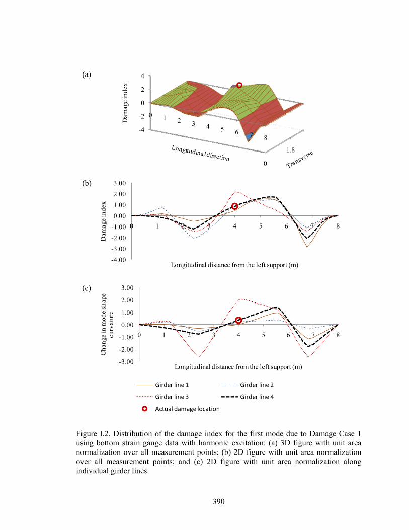
390
-3.00
-2.00
-1.00
0.00
1.00
2.00
3.00
0 1 2 3 4 5 6 7 8
Cha
nge
in m
ode
shap
e cu
rvat
ure
Longitudinal distance from the left support (m)
Girder line 1 Girder line 2
Girder line 3 Girder line 4
Actual damage location
-4.00
-3.00
-2.00
-1.00
0.00
1.00
2.00
3.00
0 1 2 3 4 5 6 7 8
Dam
age
inde
x
Longitudinal distance from the left support (m)
0
1.8
-4
-2
0
2
4
0 1 2 3 4 5 6 7 8
Dam
age
inde
x
Figure I.2. Distribution of the damage index for the first mode due to Damage Case 1using bottom strain gauge data with harmonic excitation: (a) 3D figure with unit areanormalization over all measurement points; (b) 2D figure with unit area normalizationover all measurement points; and (c) 2D figure with unit area normalization alongindividual girder lines.
(a)
(c)
(b)

391
-0.03
-0.02
-0.01
0.00
0.01
0.02
0.03
0 1 2 3 4 5 6 7 8
Cha
nge
in m
ode
shap
e
Longitudinal distance from the left support (m)
Girder line 1 Girder line 2
Girder line 3 Girder line 4
Actual damage location
-0.20
-0.15
-0.10
-0.05
0.00
0.05
0.10
0.15
0.20
0 1 2 3 4 5 6 7 8
Cha
nge
in m
ode
shap
e
Longitudinal distance from the left support (m)
0
1.8
-0.2
-0.1
0
0.1
0.2
0 1 2 3 4 5 6 7 8
Cha
nge
in m
ode
shap
e
Figure I.3. Distribution of the change in the first mode shape due to Damage Case 1using middle strain gauge data with harmonic excitation: (a) 3D figure with unit areanormalization over all measurement points; (b) 2D figure with unit area normalizationover all measurement points; and (c) 2D figure with unit area normalization alongindividual girder lines.
(a)
(c)
(b)
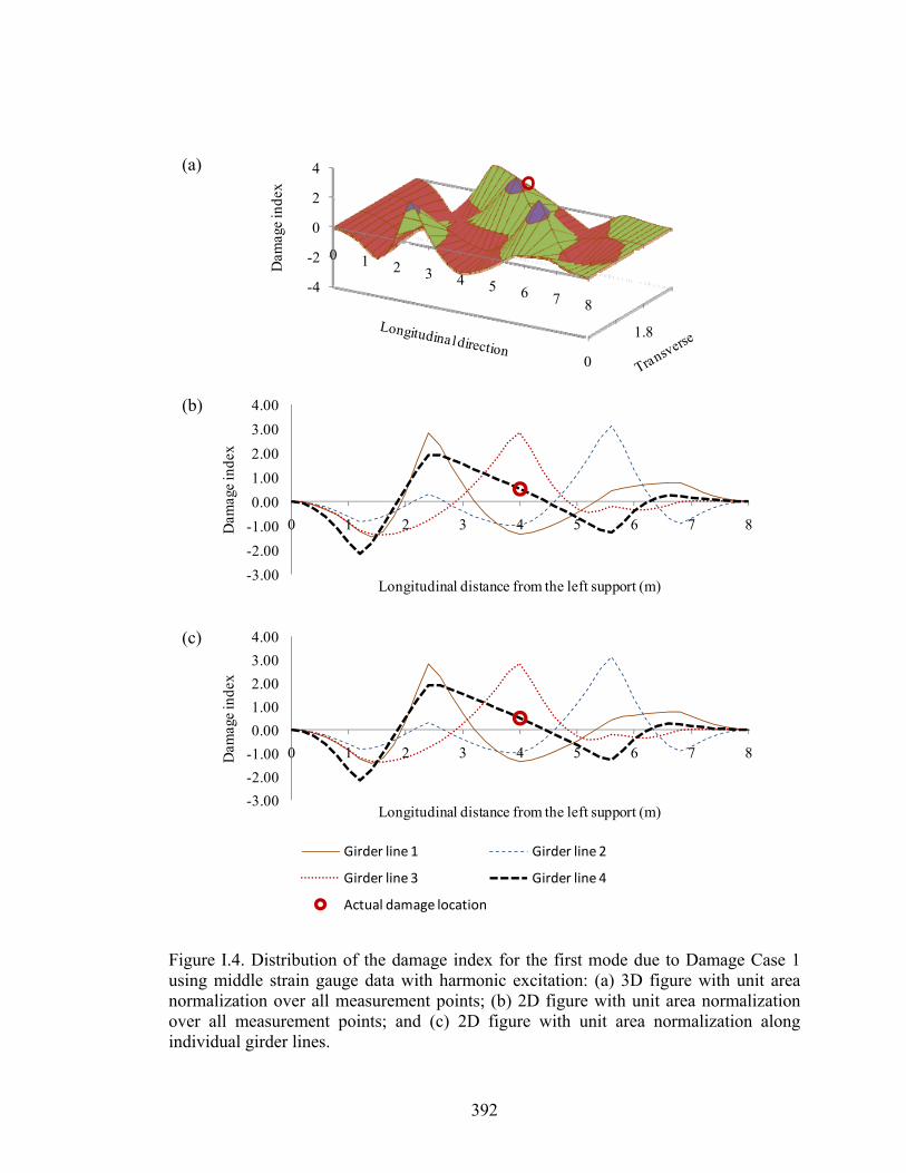
392
-3.00
-2.00
-1.00
0.00
1.00
2.00
3.00
4.00
0 1 2 3 4 5 6 7 8Dam
age
inde
x
Longitudinal distance from the left support (m)
Girder line 1 Girder line 2
Girder line 3 Girder line 4
Actual damage location
-3.00
-2.00
-1.00
0.00
1.00
2.00
3.00
4.00
0 1 2 3 4 5 6 7 8Dam
age
inde
x
Longitudinal distance from the left support (m)
0
1.8
-4
-2
0
2
4
0 1 2 3 4 5 6 7 8
Dam
age
inde
x
Figure I.4. Distribution of the damage index for the first mode due to Damage Case 1using middle strain gauge data with harmonic excitation: (a) 3D figure with unit areanormalization over all measurement points; (b) 2D figure with unit area normalizationover all measurement points; and (c) 2D figure with unit area normalization alongindividual girder lines.
(a)
(c)
(b)

393
-3.00
-2.00
-1.00
0.00
1.00
2.00
3.00
0 1 2 3 4 5 6 7 8
Cha
nge
in m
ode
shap
e cu
rvat
ure
Longitudinal distance from the left support (m)
Girder line 1 Girder line 2
Girder line 3 Girder line 4
Actual damage location
-3.00
-2.00
-1.00
0.00
1.00
2.00
3.00
4.00
0 1 2 3 4 5 6 7 8
Cha
nge
in m
ode
shap
e cu
rvat
ure
Longitudinal distance from the left support (m)
Figure I.5. Distribution of the change in mode shape curvature for the first mode due toDamage Case 1 using middle strain gauge data with harmonic excitation: (a) 3D figurewith unit area normalization over all measurement points; (b) 2D figure with unit areanormalization over all measurement points; and (c) 2D figure with unit areanormalization along individual girder lines.
(a)
(c)
(b)
0
1.8
-4
-2
0
2
4
0 1 2 3 4 5 6 7 8
Cha
nge
in m
ode
shap
ecu
rvat
ure

394
-0.20
-0.15
-0.10
-0.05
0.00
0.05
0.10
0.15
0 1 2 3 4 5 6 7 8
Cha
nge
in m
ode
shap
e
Longitudinal distance from the left support (m)
Girder line 1 Girder line 2
Girder line 3 Girder line 4
Actual damage location
-0.30
-0.20
-0.10
0.00
0.10
0.20
0.30
0 1 2 3 4 5 6 7 8
Cha
nge
in m
ode
shap
e
Longitudinal distance from the left support (m)
0
1.8
-0.2
-0.1
0
0.1
0.2
0 1 2 3 4 5 6 7 8
Cha
nge
in m
ode
shap
e
Figure I.6. Distribution of the change in the first mode shape due to Damage Case 1using top strain gauge data with harmonic excitation: (a) 3D figure with unit areanormalization over all measurement points; (b) 2D figure with unit area normalizationover all measurement points; and (c) 2D figure with unit area normalization alongindividual girder lines.
(a)
(c)
(b)

395
-4.00-3.00-2.00-1.000.001.002.003.004.00
0 1 2 3 4 5 6 7 8
Dam
age
inde
x
Longitudinal distance from the left support (m)
Girder line 1 Girder line 2
Girder line 3 Girder line 4
Actual damage location
-4.00
-3.00
-2.00
-1.00
0.00
1.00
2.00
3.00
4.00
0 1 2 3 4 5 6 7 8
Dam
age
inde
x
Longitudinal distance from the left support (m)
0
1.8
-4
-2
0
2
4
0 1 2 3 4 5 6 7 8
Dam
age
inde
x
Figure I.7. Distribution of the damage index for the first mode due to Damage Case 1using top strain gauge data with harmonic excitation: (a) 3D figure with unit areanormalization over all measurement points; (b) 2D figure with unit area normalizationover all measurement points; and (c) 2D figure with unit area normalization alongindividual girder lines.
(a)
(c)
(b)
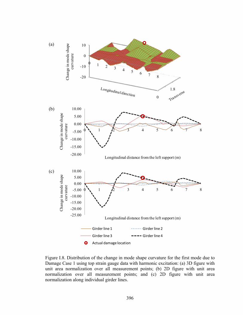
396
-25.00
-20.00
-15.00
-10.00
-5.00
0.00
5.00
10.00
0 1 2 3 4 5 6 7 8
Cha
nge
in m
ode
shap
e cu
rvat
ure
Longitudinal distance from the left support (m)
Girder line 1 Girder line 2
Girder line 3 Girder line 4
Actual damage location
-20.00
-15.00
-10.00
-5.00
0.00
5.00
10.00
0 1 2 3 4 5 6 7 8
Cha
nge
in m
ode
shap
e cu
rvat
ure
Longitudinal distance from the left support (m)
0
1.8
-20
-10
0
10
0 1 2 3 4 5 6 7 8
Cha
nge
in m
ode
shap
ecu
rvat
ure
Figure I.8. Distribution of the change in mode shape curvature for the first mode due toDamage Case 1 using top strain gauge data with harmonic excitation: (a) 3D figure withunit area normalization over all measurement points; (b) 2D figure with unit areanormalization over all measurement points; and (c) 2D figure with unit areanormalization along individual girder lines.
(a)
(c)
(b)
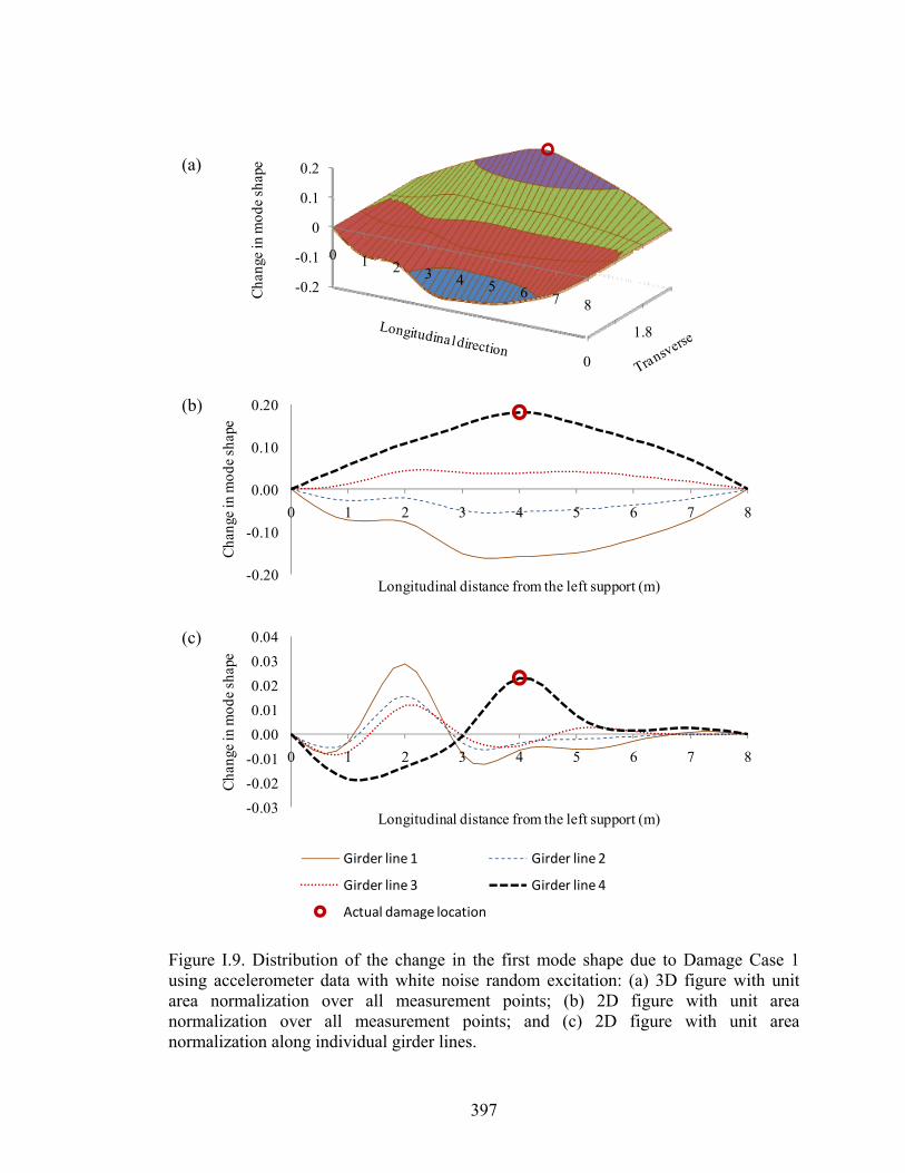
397
-0.20
-0.10
0.00
0.10
0.20
0 1 2 3 4 5 6 7 8
Cha
nge
in m
ode
shap
e
Longitudinal distance from the left support (m)
0
1.8
-0.2
-0.1
0
0.1
0.2
0 1 2 3 4 5 6 7 8
Cha
nge
in m
ode
shap
e
-0.03
-0.02
-0.01
0.00
0.01
0.02
0.03
0.04
0 1 2 3 4 5 6 7 8
Cha
nge
in m
ode
shap
e
Longitudinal distance from the left support (m)
Girder line 1 Girder line 2
Girder line 3 Girder line 4
Actual damage location
Figure I.9. Distribution of the change in the first mode shape due to Damage Case 1using accelerometer data with white noise random excitation: (a) 3D figure with unitarea normalization over all measurement points; (b) 2D figure with unit areanormalization over all measurement points; and (c) 2D figure with unit areanormalization along individual girder lines.
(a)
(c)
(b)
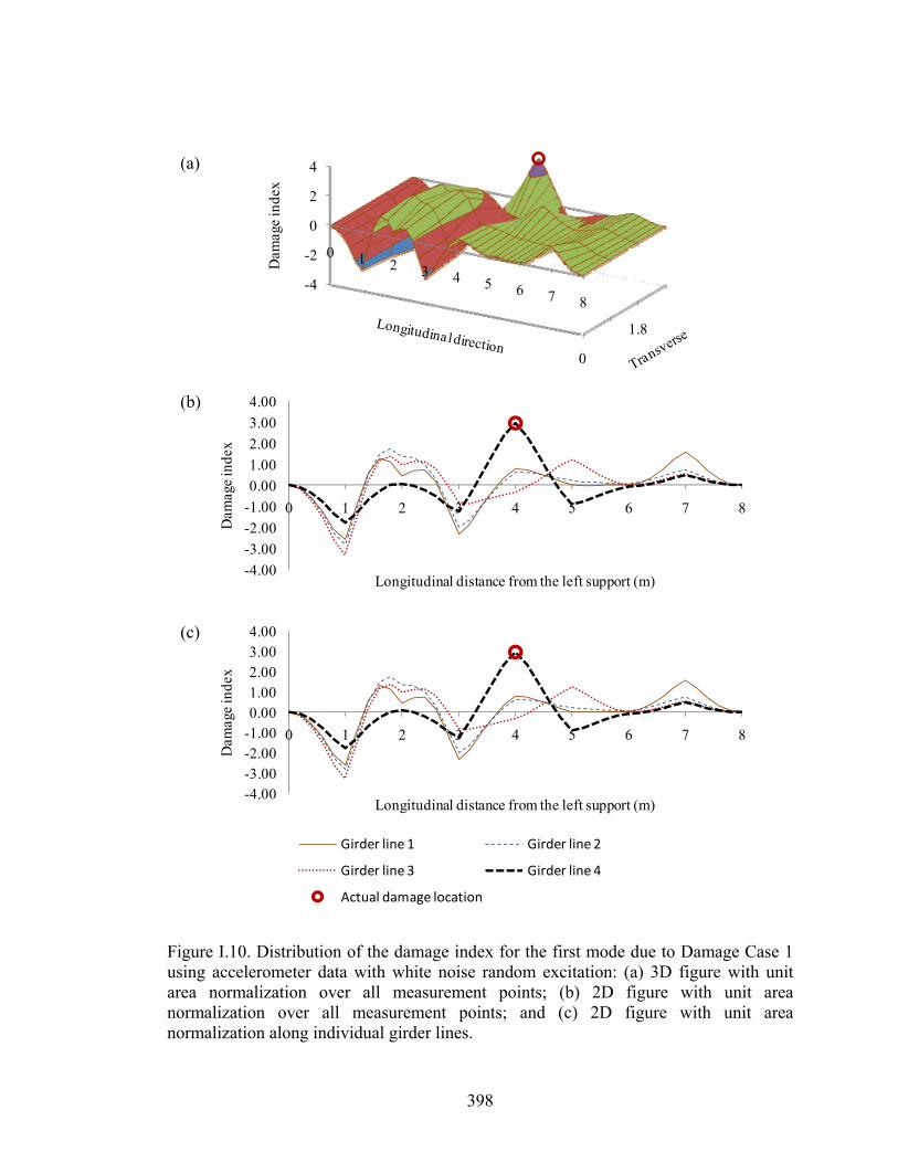
398
-4.00
-3.00
-2.00
-1.00
0.00
1.00
2.00
3.00
4.00
0 1 2 3 4 5 6 7 8
Dam
age
inde
x
Longitudinal distance from the left support (m)
-4.00-3.00-2.00-1.000.001.002.003.004.00
0 1 2 3 4 5 6 7 8
Dam
age
inde
x
Longitudinal distance from the left support (m)
Girder line 1 Girder line 2
Girder line 3 Girder line 4
Actual damage location
0
1.8
-4
-2
0
2
4
0 1 2 3 4 5 6 7 8
Dam
age
inde
x
Figure I.10. Distribution of the damage index for the first mode due to Damage Case 1using accelerometer data with white noise random excitation: (a) 3D figure with unitarea normalization over all measurement points; (b) 2D figure with unit areanormalization over all measurement points; and (c) 2D figure with unit areanormalization along individual girder lines.
(a)
(c)
(b)
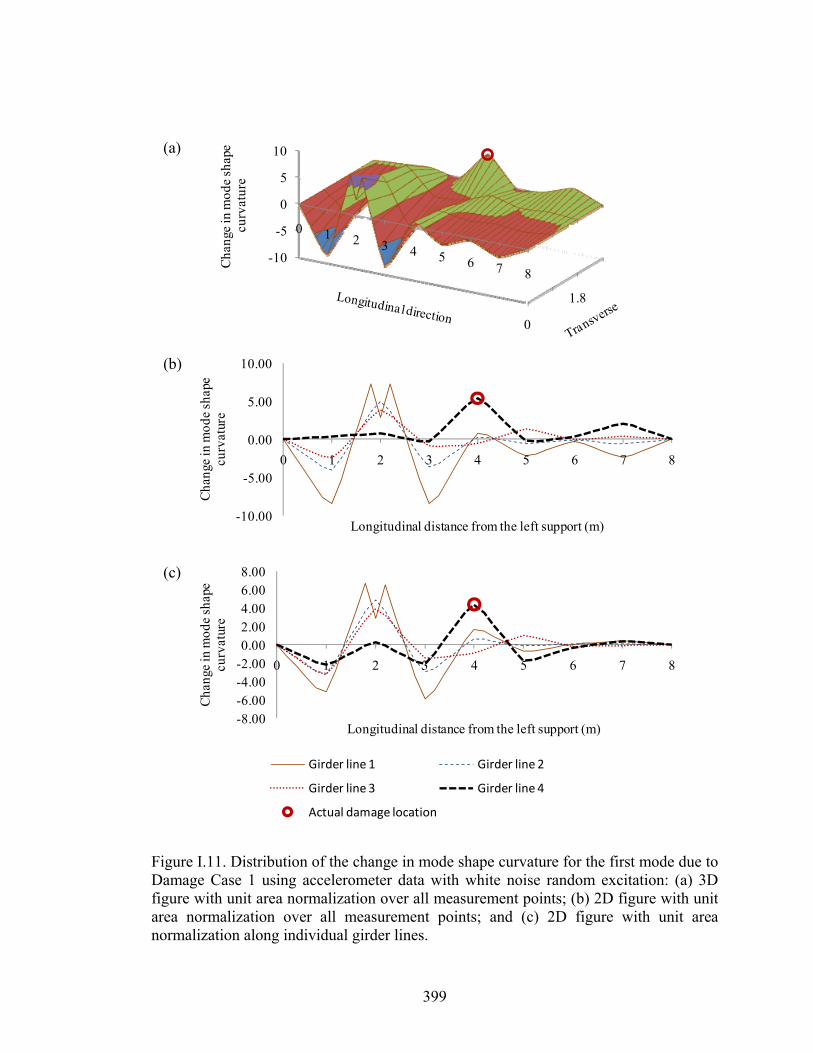
399
-10.00
-5.00
0.00
5.00
10.00
0 1 2 3 4 5 6 7 8
Cha
nge
in m
ode
shap
e cu
rvat
ure
Longitudinal distance from the left support (m)
0
1.8
-10
-5
0
5
10
0 1 2 3 4 5 6 7 8
Cha
nge
in m
ode
shap
ecu
rvat
ure
-8.00-6.00-4.00-2.000.002.004.006.008.00
0 1 2 3 4 5 6 7 8
Cha
nge
in m
ode
shap
e cu
rvat
ure
Longitudinal distance from the left support (m)
Girder line 1 Girder line 2
Girder line 3 Girder line 4
Actual damage location
Figure I.11. Distribution of the change in mode shape curvature for the first mode due toDamage Case 1 using accelerometer data with white noise random excitation: (a) 3Dfigure with unit area normalization over all measurement points; (b) 2D figure with unitarea normalization over all measurement points; and (c) 2D figure with unit areanormalization along individual girder lines.
(a)
(c)
(b)

400
APPENDIX J. DETECTION OF DAMAGE CASE 1 USING
HIGHER VIBRATION MODES WHEN
ACCELEROMETER DATA AND WHITE NOISE
RANDOM EXCITATION WERE USED
This appendix presents additional information for Section 6.3, providing damage
localization of Damage Case 1 using commonly available VBDD indicators, based on
the higher vibration modes extracted from accelerometer data (i.e., the 2nd, 3rd, 4th, and
5th modes), when white noise random excitation was used. The damage indicators used
in this Appendix included change in mode shape method, damage index method, and
change in mode shape curvature method.
Figures J.1 to J.4 present the results of damage localization using the change in mode
shape method, when Test Protocols 13, 17, 21, and 25 were used, respectively.
Figures J.5 to J.8 present the results of damage localization using the damage index
method, when Test Protocols 13, 17, 21, and 25 were used, respectively.
Figures J.9 to J.12 present the results of damage localization using the change in mode
shape curvature method, when Test Protocols 13, 17, 21, and 25 were used, respectively.
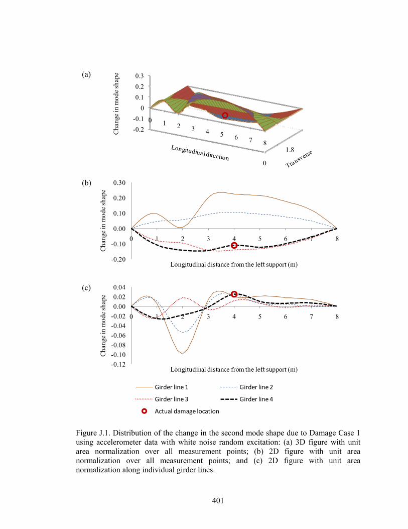
401
-0.12
-0.10
-0.08
-0.06
-0.04
-0.02
0.00
0.02
0.04
0 1 2 3 4 5 6 7 8
Cha
nge
in m
ode
shap
e
Longitudinal distance from the left support (m)
Girder line 1 Girder line 2
Girder line 3 Girder line 4
Actual damage location
-0.20
-0.10
0.00
0.10
0.20
0.30
0 1 2 3 4 5 6 7 8
Cha
nge
in m
ode
shap
e
Longitudinal distance from the left support (m)
0
1.8
-0.2
-0.1
0
0.1
0.2
0.3
0 1 2 3 4 5 6 7 8
Cha
nge
in m
ode
shap
e
Figure J.1. Distribution of the change in the second mode shape due to Damage Case 1using accelerometer data with white noise random excitation: (a) 3D figure with unitarea normalization over all measurement points; (b) 2D figure with unit areanormalization over all measurement points; and (c) 2D figure with unit areanormalization along individual girder lines.
(a)
(c)
(b)
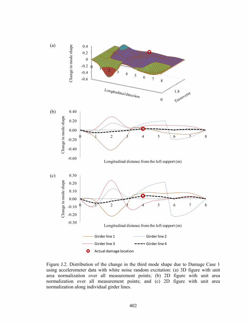
402
-0.30
-0.20
-0.10
0.00
0.10
0.20
0.30
0 1 2 3 4 5 6 7 8
Cha
nge
in m
ode
shap
e
Longitudinal distance from the left support (m)
Girder line 1 Girder line 2
Girder line 3 Girder line 4
Actual damage location
-0.60
-0.40
-0.20
0.00
0.20
0.40
0 1 2 3 4 5 6 7 8
Cha
nge
in m
ode
shap
e
Longitudinal distance from the left support (m)
0
1.8
-0.6
-0.4
-0.2
0
0.2
0.4
0 1 2 3 4 5 6 7 8Cha
nge
in m
ode
shap
e
Figure J.2. Distribution of the change in the third mode shape due to Damage Case 1using accelerometer data with white noise random excitation: (a) 3D figure with unitarea normalization over all measurement points; (b) 2D figure with unit areanormalization over all measurement points; and (c) 2D figure with unit areanormalization along individual girder lines.
(a)
(c)
(b)
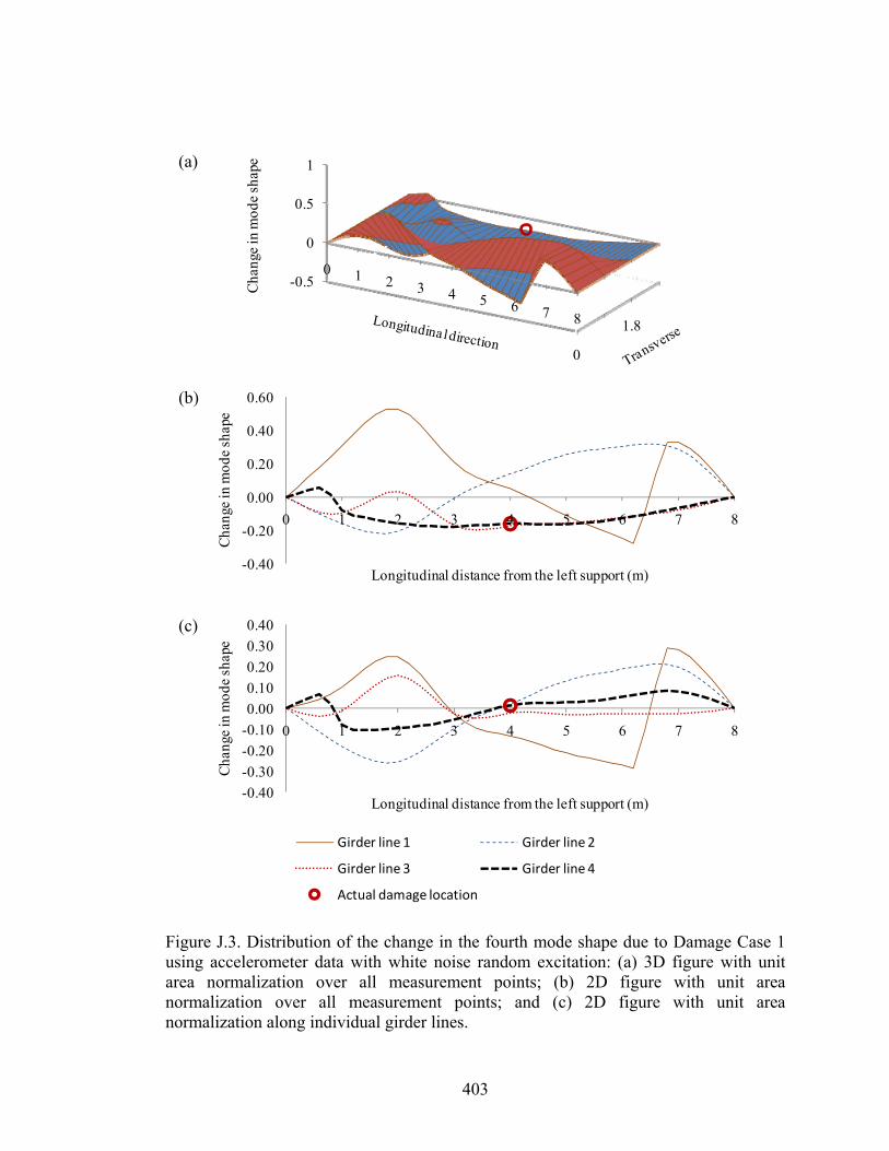
403
-0.40
-0.30
-0.20
-0.10
0.00
0.10
0.20
0.30
0.40
0 1 2 3 4 5 6 7 8
Cha
nge
in m
ode
shap
e
Longitudinal distance from the left support (m)
Girder line 1 Girder line 2
Girder line 3 Girder line 4
Actual damage location
-0.40
-0.20
0.00
0.20
0.40
0.60
0 1 2 3 4 5 6 7 8
Cha
nge
in m
ode
shap
e
Longitudinal distance from the left support (m)
0
1.8
-0.5
0
0.5
1
0 1 2 3 4 5 6 7 8
Cha
nge
in m
ode
shap
e
Figure J.3. Distribution of the change in the fourth mode shape due to Damage Case 1using accelerometer data with white noise random excitation: (a) 3D figure with unitarea normalization over all measurement points; (b) 2D figure with unit areanormalization over all measurement points; and (c) 2D figure with unit areanormalization along individual girder lines.
(a)
(c)
(b)
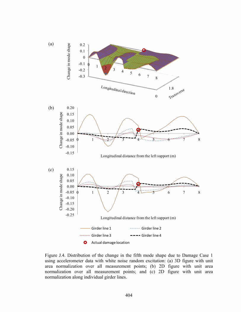
404
0
1.8
-0.3
-0.2
-0.1
0
0.1
0.2
0 1 2 3 4 5 6 7 8Cha
nge
in m
ode
shap
e
-0.25
-0.20
-0.15
-0.10
-0.05
0.00
0.05
0.10
0.15
0 1 2 3 4 5 6 7 8
Cha
nge
in m
ode
shap
e
Longitudinal distance from the left support (m)
Girder line 1 Girder line 2
Girder line 3 Girder line 4
Actual damage location
-0.15
-0.10
-0.05
0.00
0.05
0.10
0.15
0.20
0 1 2 3 4 5 6 7 8
Cha
nge
in m
ode
shap
e
Longitudinal distance from the left support (m)
Figure J.4. Distribution of the change in the fifth mode shape due to Damage Case 1using accelerometer data with white noise random excitation: (a) 3D figure with unitarea normalization over all measurement points; (b) 2D figure with unit areanormalization over all measurement points; and (c) 2D figure with unit areanormalization along individual girder lines.
(a)
(c)
(b)

405
-6.00
-4.00
-2.00
0.00
2.00
4.00
0 1 2 3 4 5 6 7 8
Dam
age
inde
x
Longitudinal distance from the left support (m)
Girder line 1 Girder line 2
Girder line 3 Girder line 4
Actual damage location
-6.00
-4.00
-2.00
0.00
2.00
4.00
0 1 2 3 4 5 6 7 8
Dam
age
inde
x
Longitudinal distance from the left support (m)
0
1.8
-4
-2
0
2
4
0 1 2 3 4 5 6 7 8
Dam
age
inde
x
Figure J.5. Distribution of the damage index for the second mode due to Damage Case 1using accelerometer data with white noise random excitation: (a) 3D figure with unitarea normalization over all measurement points; (b) 2D figure with unit areanormalization over all measurement points; and (c) 2D figure with unit areanormalization along individual girder lines.
(a)
(c)
(b)
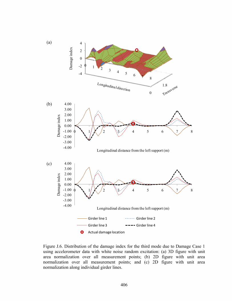
406
-4.00-3.00-2.00-1.000.001.002.003.004.00
0 1 2 3 4 5 6 7 8
Dam
age
inde
x
Longitudinal distance from the left support (m)
Girder line 1 Girder line 2
Girder line 3 Girder line 4
Actual damage location
-4.00
-3.00
-2.00
-1.00
0.00
1.00
2.00
3.00
4.00
0 1 2 3 4 5 6 7 8
Dam
age
inde
x
Longitudinal distance from the left support (m)
0
1.8
-4
-2
0
2
4
0 1 2 3 4 5 6 7 8
Dam
age
inde
x
Figure J.6. Distribution of the damage index for the third mode due to Damage Case 1using accelerometer data with white noise random excitation: (a) 3D figure with unitarea normalization over all measurement points; (b) 2D figure with unit areanormalization over all measurement points; and (c) 2D figure with unit areanormalization along individual girder lines.
(a)
(c)
(b)
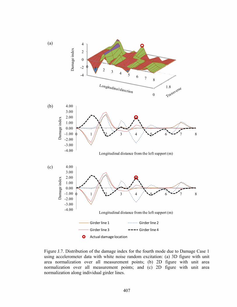
407
-4.00-3.00-2.00-1.000.001.002.003.004.00
0 1 2 3 4 5 6 7 8
Dam
age
inde
x
Longitudinal distance from the left support (m)
Girder line 1 Girder line 2
Girder line 3 Girder line 4
Actual damage location
-4.00
-3.00
-2.00
-1.00
0.00
1.00
2.00
3.00
4.00
0 1 2 3 4 5 6 7 8
Dam
age
inde
x
Longitudinal distance from the left support (m)
0
1.8
-4
-2
0
2
4
0 1 2 3 4 5 6 7 8
Dam
age
inde
x
Figure J.7. Distribution of the damage index for the fourth mode due to Damage Case 1using accelerometer data with white noise random excitation: (a) 3D figure with unitarea normalization over all measurement points; (b) 2D figure with unit areanormalization over all measurement points; and (c) 2D figure with unit areanormalization along individual girder lines.
(a)
(c)
(b)
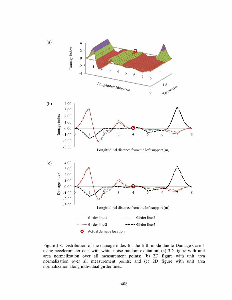
408
-3.00
-2.00
-1.00
0.00
1.00
2.00
3.00
4.00
0 1 2 3 4 5 6 7 8Dam
age
inde
x
Longitudinal distance from the left support (m)
Girder line 1 Girder line 2
Girder line 3 Girder line 4
Actual damage location
-3.00
-2.00
-1.00
0.00
1.00
2.00
3.00
4.00
0 1 2 3 4 5 6 7 8Dam
age
inde
x
Longitudinal distance from the left support (m)
0
1.8
-4
-2
0
2
4
0 1 2 3 4 5 6 7 8
Dam
age
inde
x
Figure J.8. Distribution of the damage index for the fifth mode due to Damage Case 1using accelerometer data with white noise random excitation: (a) 3D figure with unitarea normalization over all measurement points; (b) 2D figure with unit areanormalization over all measurement points; and (c) 2D figure with unit areanormalization along individual girder lines.
(a)
(c)
(b)
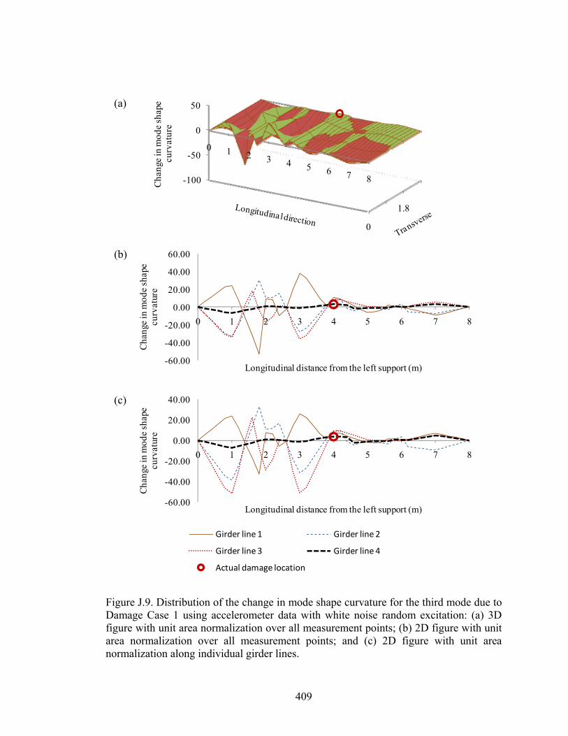
409
-60.00
-40.00
-20.00
0.00
20.00
40.00
0 1 2 3 4 5 6 7 8
Cha
nge
in m
ode
shap
e cu
rvat
ure
Longitudinal distance from the left support (m)
Girder line 1 Girder line 2
Girder line 3 Girder line 4
Actual damage location
-60.00
-40.00
-20.00
0.00
20.00
40.00
60.00
0 1 2 3 4 5 6 7 8
Cha
nge
in m
ode
shap
e cu
rvat
ure
Longitudinal distance from the left support (m)
0
1.8
-100
-50
0
50
0 1 2 3 4 5 6 7 8
Cha
nge
in m
ode
shap
ecu
rvat
ure
Figure J.9. Distribution of the change in mode shape curvature for the third mode due toDamage Case 1 using accelerometer data with white noise random excitation: (a) 3Dfigure with unit area normalization over all measurement points; (b) 2D figure with unitarea normalization over all measurement points; and (c) 2D figure with unit areanormalization along individual girder lines.
(a)
(c)
(b)
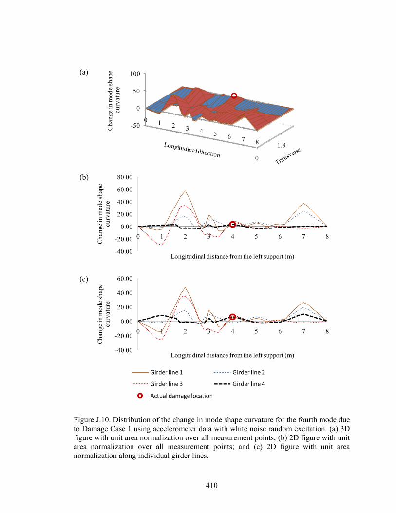
410
-40.00
-20.00
0.00
20.00
40.00
60.00
0 1 2 3 4 5 6 7 8
Cha
nge
in m
ode
shap
e cu
rvat
ure
Longitudinal distance from the left support (m)
Girder line 1 Girder line 2
Girder line 3 Girder line 4
Actual damage location
-40.00
-20.00
0.00
20.00
40.00
60.00
80.00
0 1 2 3 4 5 6 7 8
Cha
nge
in m
ode
shap
e cu
rvat
ure
Longitudinal distance from the left support (m)
0
1.8
-50
0
50
100
0 1 2 3 4 5 6 7 8
Cha
nge
in m
ode
shap
ecu
rvat
ure
Figure J.10. Distribution of the change in mode shape curvature for the fourth mode dueto Damage Case 1 using accelerometer data with white noise random excitation: (a) 3Dfigure with unit area normalization over all measurement points; (b) 2D figure with unitarea normalization over all measurement points; and (c) 2D figure with unit areanormalization along individual girder lines.
(a)
(c)
(b)

411
-80.00
-60.00
-40.00
-20.00
0.00
20.00
40.00
60.00
0 1 2 3 4 5 6 7 8
Cha
nge
in m
ode
shap
e cu
rvat
ure
Longitudinal distance from the left support (m)
Girder line 1 Girder line 2
Girder line 3 Girder line 4
Actual damage location
-60.00
-40.00
-20.00
0.00
20.00
40.00
60.00
0 1 2 3 4 5 6 7 8
Cha
nge
in m
ode
shap
e cu
rvat
ure
Longitudinal distance from the left support (m)
0
1.8
-50
0
50
0 1 2 3 4 5 6 7 8
Cha
nge
in m
ode
shap
ecu
rvat
ure
Figure J.11. Distribution of the change in mode shape curvature for the fifth mode dueto Damage Case 1 using accelerometer data with white noise random excitation: (a) 3Dfigure with unit area normalization over all measurement points; (b) 2D figure with unitarea normalization over all measurement points; and (c) 2D figure with unit areanormalization along individual girder lines.
(a)
(c)
(b)

412
APPENDIX K. DAMAGE DETECTION USING CHANGE
IN THE FIRST MODE SHAPE FOR DAMAGE CASES 2
TO 16 WHEN ACCELEROMETER DATA AND
HARMONIC EXCITATION WERE USED
This appendix presents additional information for Section 6.3, providing damage
localization of Damage Cases 2 to 16 using the change in mode shape method, when
Test Protocol 1 was used, which are similar to results presented in Fig. 6.17.

413
0
1.8
-0.05
0
0.05
0.1
0 1 2 3 4 5 6 7 8
Cha
nge
in m
ode
shap
e
Figure K.1. Distribution of the change in the first mode shape due to Damage Case 2using accelerometer data with harmonic excitation: (a) 3D figure with unit areanormalization over all measurement points; (b) 2D figure with unit area normalizationover all measurement points; and (c) 2D figure with unit area normalization alongindividual girder lines.
(a)
(c)
(b)
-0.06
-0.04
-0.02
0.00
0.02
0.04
0.06
0.08
0 1 2 3 4 5 6 7 8
Cha
nge
in m
ode
shap
e
Longitudinal distance from the left support (m)
-0.05
-0.04
-0.03
-0.02
-0.01
0.00
0.01
0.02
0 1 2 3 4 5 6 7 8
Cha
nge
in m
ode
shap
e
Longitudinal distance from the left support (m)
Girder line 1 Girder line 2
Girder line 3 Girder line 4
Actual damage location
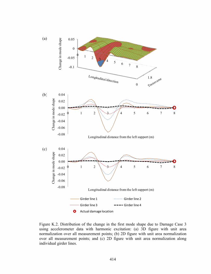
414
0
1.8
-0.1
-0.05
0
0.05
0 1 2 3 4 5 6 7 8
Cha
nge
in m
ode
shap
e
Figure K.2. Distribution of the change in the first mode shape due to Damage Case 3using accelerometer data with harmonic excitation: (a) 3D figure with unit areanormalization over all measurement points; (b) 2D figure with unit area normalizationover all measurement points; and (c) 2D figure with unit area normalization alongindividual girder lines.
(a)
(c)
(b)
-0.08
-0.06
-0.04
-0.02
0.00
0.02
0.04
0 1 2 3 4 5 6 7 8
Cha
nge
in m
ode
shap
e
Longitudinal distance from the left support (m)
-0.08
-0.06
-0.04
-0.02
0.00
0.02
0.04
0 1 2 3 4 5 6 7 8
Cha
nge
in m
ode
shap
e
Longitudinal distance from the left support (m)
Girder line 1 Girder line 2
Girder line 3 Girder line 4
Actual damage location

415
0
1.8
-0.05
0
0.05
0.1
0 1 2 3 4 5 6 7 8
Cha
nge
in m
ode
shap
e
Figure K.3. Distribution of the change in the first mode shape due to Damage Case 4using accelerometer data with harmonic excitation: (a) 3D figure with unit areanormalization over all measurement points; (b) 2D figure with unit area normalizationover all measurement points; and (c) 2D figure with unit area normalization alongindividual girder lines.
(a)
(c)
(b)
-0.05
0.00
0.05
0.10
0.15
0 1 2 3 4 5 6 7 8Cha
nge
in m
ode
shap
e
Longitudinal distance from the left support (m)
-0.04
-0.02
0.00
0.02
0.04
0.06
0.08
0 1 2 3 4 5 6 7 8
Cha
nge
in m
ode
shap
e
Longitudinal distance from the left support (m)
Girder line 1 Girder line 2
Girder line 3 Girder line 4
Actual damage location
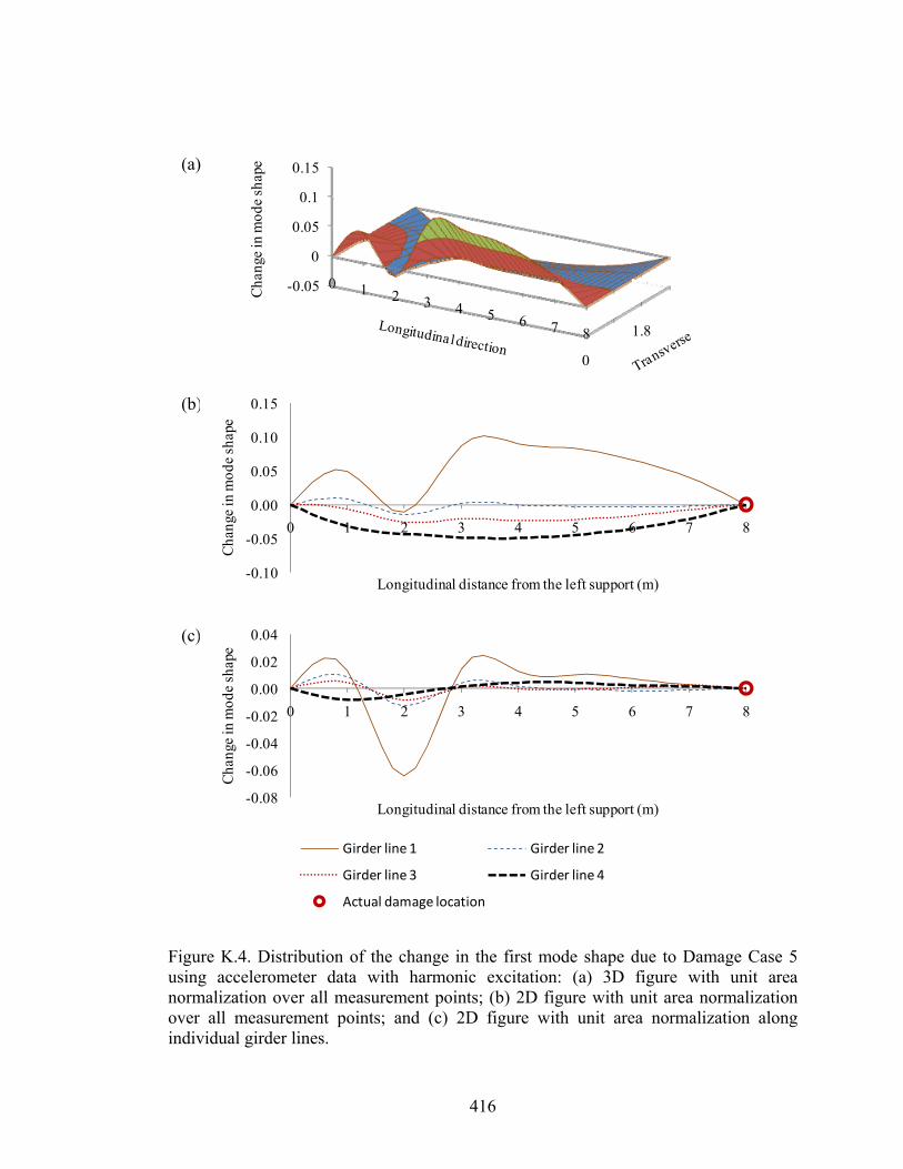
416
0
1.8
-0.05
0
0.05
0.1
0.15
0 1 2 3 4 5 6 7 8
Cha
nge
in m
ode
shap
e
Figure K.4. Distribution of the change in the first mode shape due to Damage Case 5using accelerometer data with harmonic excitation: (a) 3D figure with unit areanormalization over all measurement points; (b) 2D figure with unit area normalizationover all measurement points; and (c) 2D figure with unit area normalization alongindividual girder lines.
(a)
(c)
(b)
-0.10
-0.05
0.00
0.05
0.10
0.15
0 1 2 3 4 5 6 7 8
Cha
nge
in m
ode
shap
e
Longitudinal distance from the left support (m)
-0.08
-0.06
-0.04
-0.02
0.00
0.02
0.04
0 1 2 3 4 5 6 7 8
Cha
nge
in m
ode
shap
e
Longitudinal distance from the left support (m)
Girder line 1 Girder line 2
Girder line 3 Girder line 4
Actual damage location
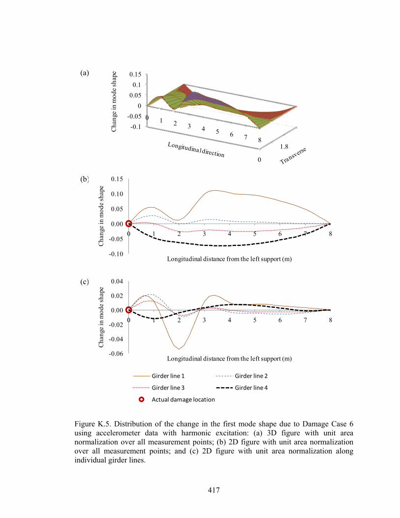
417
0
1.8
-0.1
-0.05
0
0.05
0.1
0.15
0 1 2 3 4 5 6 7 8
Cha
nge
in m
ode
shap
e
Figure K.5. Distribution of the change in the first mode shape due to Damage Case 6using accelerometer data with harmonic excitation: (a) 3D figure with unit areanormalization over all measurement points; (b) 2D figure with unit area normalizationover all measurement points; and (c) 2D figure with unit area normalization alongindividual girder lines.
(a)
(c)
(b)
-0.10
-0.05
0.00
0.05
0.10
0.15
0 1 2 3 4 5 6 7 8
Cha
nge
in m
ode
shap
e
Longitudinal distance from the left support (m)
-0.06
-0.04
-0.02
0.00
0.02
0.04
0 1 2 3 4 5 6 7 8
Cha
nge
in m
ode
shap
e
Longitudinal distance from the left support (m)
Girder line 1 Girder line 2
Girder line 3 Girder line 4
Actual damage location
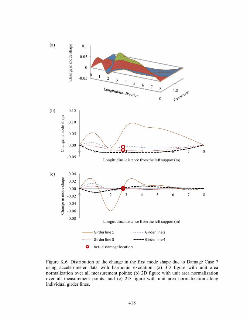
418
0
1.8
-0.05
0
0.05
0.1
0 1 2 3 4 5 6 7 8
Cha
nge
in m
ode
shap
e
Figure K.6. Distribution of the change in the first mode shape due to Damage Case 7using accelerometer data with harmonic excitation: (a) 3D figure with unit areanormalization over all measurement points; (b) 2D figure with unit area normalizationover all measurement points; and (c) 2D figure with unit area normalization alongindividual girder lines.
(a)
(c)
(b)
-0.05
0.00
0.05
0.10
0.15
0 1 2 3 4 5 6 7 8Cha
nge
in m
ode
shap
e
Longitudinal distance from the left support (m)
-0.08
-0.06
-0.04
-0.02
0.00
0.02
0.04
0 1 2 3 4 5 6 7 8
Cha
nge
in m
ode
shap
e
Longitudinal distance from the left support (m)
Girder line 1 Girder line 2
Girder line 3 Girder line 4
Actual damage location
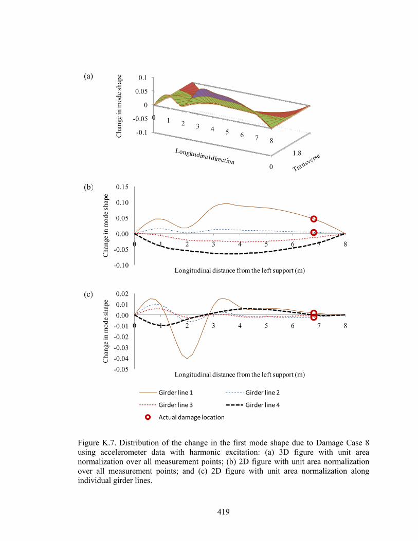
419
0
1.8
-0.1
-0.05
0
0.05
0.1
0 1 2 3 4 5 6 7 8
Cha
nge
in m
ode
shap
e
Figure K.7. Distribution of the change in the first mode shape due to Damage Case 8using accelerometer data with harmonic excitation: (a) 3D figure with unit areanormalization over all measurement points; (b) 2D figure with unit area normalizationover all measurement points; and (c) 2D figure with unit area normalization alongindividual girder lines.
(a)
(c)
(b)
-0.10
-0.05
0.00
0.05
0.10
0.15
0 1 2 3 4 5 6 7 8
Cha
nge
in m
ode
shap
e
Longitudinal distance from the left support (m)
-0.05
-0.04
-0.03
-0.02
-0.01
0.00
0.01
0.02
0 1 2 3 4 5 6 7 8
Cha
nge
in m
ode
shap
e
Longitudinal distance from the left support (m)
Girder line 1 Girder line 2
Girder line 3 Girder line 4
Actual damage location

420
0
1.8
-0.1
-0.05
0
0.05
0.1
0 1 2 3 4 5 6 7 8
Cha
nge
in m
ode
shap
e
Figure K.8. Distribution of the change in the first mode shape due to Damage Case 9using accelerometer data with harmonic excitation: (a) 3D figure with unit areanormalization over all measurement points; (b) 2D figure with unit area normalizationover all measurement points; and (c) 2D figure with unit area normalization alongindividual girder lines.
(a)
(c)
(b)
-0.10
-0.05
0.00
0.05
0.10
0 1 2 3 4 5 6 7 8
Cha
nge
in m
ode
shap
e
Longitudinal distance from the left support (m)
-0.04
-0.03
-0.02
-0.01
0.00
0.01
0.02
0 1 2 3 4 5 6 7 8
Cha
nge
in m
ode
shap
e
Longitudinal distance from the left support (m)
Girder line 1 Girder line 2
Girder line 3 Girder line 4
Actual damage location

421
0
1.8
-0.02
0
0.02
0.04
0 1 2 3 4 5 6 7 8
Cha
nge
in m
ode
shap
e
Figure K.9. Distribution of the change in the first mode shape due to Damage Case 10using accelerometer data with harmonic excitation: (a) 3D figure with unit areanormalization over all measurement points; (b) 2D figure with unit area normalizationover all measurement points; and (c) 2D figure with unit area normalization alongindividual girder lines.
(a)
(c)
(b)
-0.02
-0.01
0.00
0.01
0.02
0.03
0 1 2 3 4 5 6 7 8
Cha
nge
in m
ode
shap
e
Longitudinal distance from the left support (m)
0.00
0.00
0.00
0.00
0.00
0.01
0 1 2 3 4 5 6 7 8
Cha
nge
in m
ode
shap
e
Longitudinal distance from the left support (m)
Girder line 1 Girder line 2
Girder line 3 Girder line 4
Actual damage location

422
0
1.8
-0.02
-0.01
0
0.01
0.02
0 1 2 3 4 5 6 7 8
Cha
nge
in m
ode
shap
e
Figure K.10. Distribution of the change in the first mode shape due to Damage Case 11using accelerometer data with harmonic excitation: (a) 3D figure with unit areanormalization over all measurement points; (b) 2D figure with unit area normalizationover all measurement points; and (c) 2D figure with unit area normalization alongindividual girder lines.
(a)
(c)
(b)
-0.02
-0.01
-0.01
0.00
0.01
0.01
0.02
0 1 2 3 4 5 6 7 8
Cha
nge
in m
ode
shap
e
Longitudinal distance from the left support (m)
-0.02
-0.01
-0.01
0.00
0.01
0 1 2 3 4 5 6 7 8
Cha
nge
in m
ode
shap
e
Longitudinal distance from the left support (m)
Girder line 1 Girder line 2
Girder line 3 Girder line 4
Actual damage location
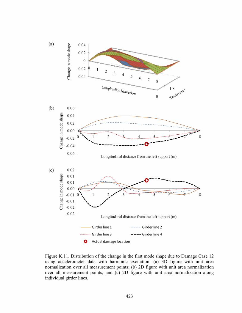
423
0
1.8
-0.04
-0.02
0
0.02
0.04
0 1 2 3 4 5 6 7 8
Cha
nge
in m
ode
shap
e
Figure K.11. Distribution of the change in the first mode shape due to Damage Case 12using accelerometer data with harmonic excitation: (a) 3D figure with unit areanormalization over all measurement points; (b) 2D figure with unit area normalizationover all measurement points; and (c) 2D figure with unit area normalization alongindividual girder lines.
(a)
(c)
(b)
-0.06
-0.04
-0.02
0.00
0.02
0.04
0.06
0 1 2 3 4 5 6 7 8
Cha
nge
in m
ode
shap
e
Longitudinal distance from the left support (m)
-0.02
-0.02
-0.01
-0.01
0.00
0.01
0.01
0.02
0 1 2 3 4 5 6 7 8
Cha
nge
in m
ode
shap
e
Longitudinal distance from the left support (m)
Girder line 1 Girder line 2
Girder line 3 Girder line 4
Actual damage location
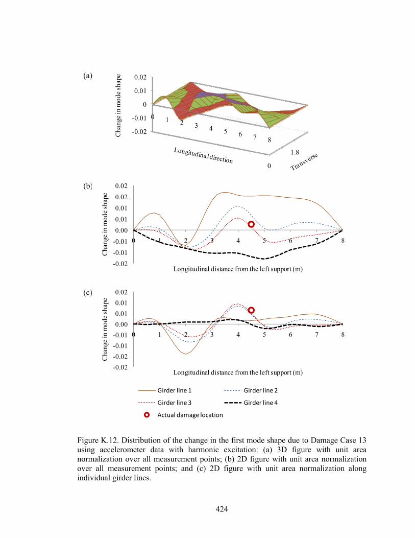
424
0
1.8
-0.02
-0.01
0
0.01
0.02
0 1 2 3 4 5 6 7 8
Cha
nge
in m
ode
shap
e
Figure K.12. Distribution of the change in the first mode shape due to Damage Case 13using accelerometer data with harmonic excitation: (a) 3D figure with unit areanormalization over all measurement points; (b) 2D figure with unit area normalizationover all measurement points; and (c) 2D figure with unit area normalization alongindividual girder lines.
(a)
(c)
(b)
-0.02
-0.01
-0.01
0.00
0.01
0.01
0.02
0.02
0 1 2 3 4 5 6 7 8
Cha
nge
in m
ode
shap
e
Longitudinal distance from the left support (m)
-0.02
-0.02
-0.01
-0.01
0.00
0.01
0.01
0.02
0 1 2 3 4 5 6 7 8
Cha
nge
in m
ode
shap
e
Longitudinal distance from the left support (m)
Girder line 1 Girder line 2
Girder line 3 Girder line 4
Actual damage location
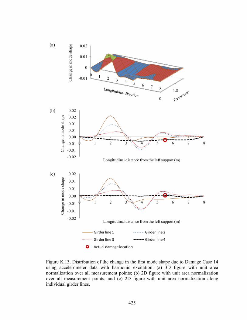
425
0
1.8
-0.01
0
0.01
0.02
0 1 2 3 4 5 6 7 8
Cha
nge
in m
ode
shap
e
Figure K.13. Distribution of the change in the first mode shape due to Damage Case 14using accelerometer data with harmonic excitation: (a) 3D figure with unit areanormalization over all measurement points; (b) 2D figure with unit area normalizationover all measurement points; and (c) 2D figure with unit area normalization alongindividual girder lines.
(a)
(c)
(b)
-0.02
-0.01
-0.01
0.00
0.01
0.01
0.02
0.02
0 1 2 3 4 5 6 7 8
Cha
nge
in m
ode
shap
e
Longitudinal distance from the left support (m)
-0.02
-0.01
-0.01
0.00
0.01
0.01
0.02
0 1 2 3 4 5 6 7 8
Cha
nge
in m
ode
shap
e
Longitudinal distance from the left support (m)
Girder line 1 Girder line 2
Girder line 3 Girder line 4
Actual damage location
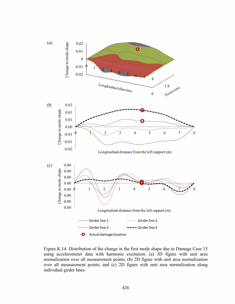
426
0
1.8
-0.02
-0.01
0
0.01
0.02
0 1 2 3 4 5 6 7 8
Cha
nge
in m
ode
shap
e
Figure K.14. Distribution of the change in the first mode shape due to Damage Case 15using accelerometer data with harmonic excitation: (a) 3D figure with unit areanormalization over all measurement points; (b) 2D figure with unit area normalizationover all measurement points; and (c) 2D figure with unit area normalization alongindividual girder lines.
(a)
(c)
(b)
-0.02
-0.01
-0.01
0.00
0.01
0.01
0.02
0 1 2 3 4 5 6 7 8
Cha
nge
in m
ode
shap
e
Longitudinal distance from the left support (m)
0.00
0.00
0.00
0.00
0.00
0.00
0.00
0.00
0 1 2 3 4 5 6 7 8
Cha
nge
in m
ode
shap
e
Longitudinal distance from the left support (m)
Girder line 1 Girder line 2
Girder line 3 Girder line 4
Actual damage location

427
0
1.8
-0.004-0.002
00.0020.0040.0060.008
0 1 2 3 4 5 6 7 8
Cha
nge
in m
ode
shap
e
Figure K.15. Distribution of the change in the first mode shape due to Damage Case 16using accelerometer data with harmonic excitation: (a) 3D figure with unit areanormalization over all measurement points; (b) 2D figure with unit area normalizationover all measurement points; and (c) 2D figure with unit area normalization alongindividual girder lines.
(a)
(c)
(b)
-0.01
0.00
0.00
0.00
0.00
0.00
0.01
0.01
0 1 2 3 4 5 6 7 8
Cha
nge
in m
ode
shap
e
Longitudinal distance from the left support (m)
0.00
0.00
0.00
0.00
0.00
0.00
0.00
0.01
0 1 2 3 4 5 6 7 8Cha
nge
in m
ode
shap
e
Longitudinal distance from the left support (m)
Girder line 1 Girder line 2
Girder line 3 Girder line 4
Actual damage location
428
APPENDIX L. USERS’ MANUAL OF PROPORTIONAL
CONTROLLER FOR HYDRAULIC VALVE
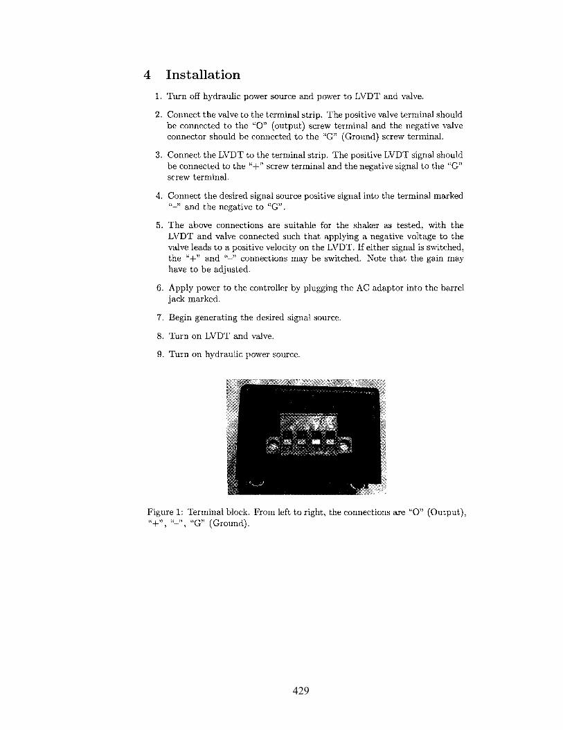
429

430

431
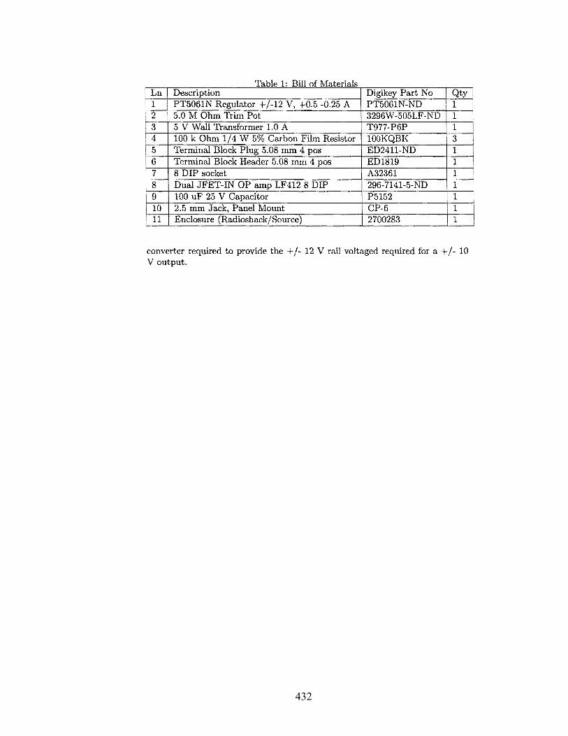
432

433
APPENDIX M. MATHCAD ROUTINES FOR DATA
PROCESSING
M.1 Overview
This appendix lists the Mathcad routines used in this study. These routines included
batch file operations for different trials in same health state, batch file operations for
different health states, file operations for interpolation and normalization, routines for
commonly available VBDD indicators, calculation of threshold values, distribution of
the area of mode shape change, calculation of the probabilities of false indicator, and a
sample calculation showing influence of different normalization schemes on the
definition of change in mode shapes and change in mode shape curvatures.

434
M.2 Batch File Operation for Different Trials in Same Health State
Notes: Define the data files and paths by specifing the dir1, dir2, dir3, and dataname, where dir2 anddataname are vectors. r is rows and c is columns to read in.
batch_read dir1 dir2 dir3 dataname r c dir21 dir2 rows dir2 0=if
dataname1 dataname rows dataname 0=if
filename concat dir1 dir2i dir3 datanamej
Mi j READFILE filename "delimited" r c
j 1 last dataname for
i 1 last dir2 for
M
Notes for summary function: 1. The purpose of this function is to summarize the results read from the batch_read function and batchwrite the summarized results to the output file which will be located in the same directory as the inputfiles;2. input files come from the batch_read function;3. dir2 and dir3 are same as the values used in batch_read function;4. output is a string value which give the filename of summarized results.
sets_summary input dir2 dir3 output summaryi inputi 1
summaryi augment summaryi inputi j
j 2 cols input for
filename concat dir2i dir3 output
WRITEPRN filename summaryi
i 1 rows input for
summary
Notes for dates_summary function:
1. input is the file read from batch_read including only mode shape information from all files;2. file1 is the first file including all information of that file;3. dir2 is testing dates.
dates_summary input file1 dir2 summary augment file1 2 file1 3 file1 4
sumi inputi 1
sumi sumi inputi j
j 2 cols input for cols input 2if
avgisumi
cols input
summary augment summary avgi
i 1 rows input for
title augment "Note" "X" "Y" dir2T
results stack title summary
results
Notes: average the results fromdifferent sets.
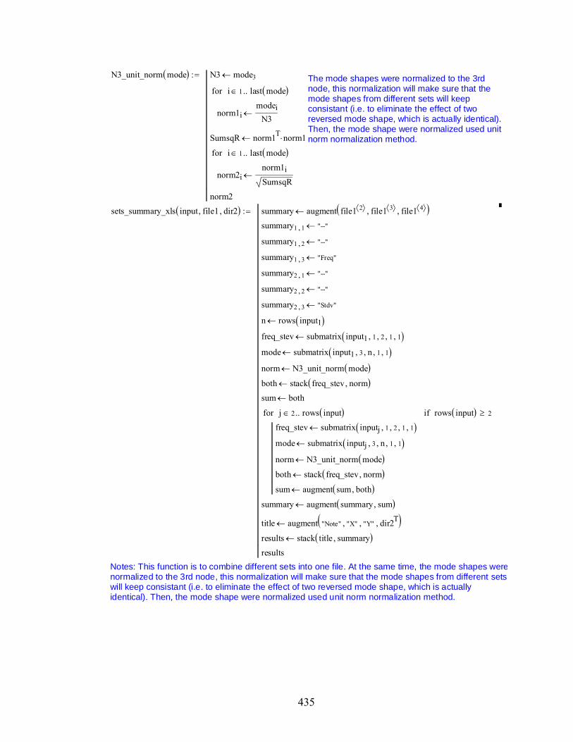
435
N3_unit_norm mode N3 mode3
norm1imodei
N3
i 1 last mode for
SumsqR norm1T norm1
norm2inorm1i
SumsqR
i 1 last mode for
norm2
The mode shapes were normalized to the 3rdnode, this normalization will make sure that themode shapes from different sets will keepconsistant (i.e. to eliminate the effect of tworeversed mode shape, which is actually identical).Then, the mode shape were normalized used unitnorm normalization method.
sets_summary_xls input file1 dir2 summary augment file1 2 file1 3 file1 4
summary1 1 "--"
summary1 2 "--"
summary1 3 "Freq"
summary2 1 "--"
summary2 2 "--"
summary2 3 "Stdv"
n rows input1
freq_stev submatrix input1 1 2 1 1
mode submatrix input1 3 n 1 1
norm N3_unit_norm mode
both stack freq_stev norm
sum both
freq_stev submatrix inputj 1 2 1 1
mode submatrix inputj 3 n 1 1
norm N3_unit_norm mode
both stack freq_stev norm
sum augment sum both
j 2 rows input for rows input 2if
summary augment summary sum
title augment "Note" "X" "Y" dir2T
results stack title summary
results
Notes: This function is to combine different sets into one file. At the same time, the mode shapes werenormalized to the 3rd node, this normalization will make sure that the mode shapes from different setswill keep consistant (i.e. to eliminate the effect of two reversed mode shape, which is actuallyidentical). Then, the mode shape were normalized used unit norm normalization method.

436
Acceleration Mode 1 with Harmonic input:
Input informations (need ajustment according different types):Testing dates, recorded sets and corresponding directories.
dir1 CWD sets1
12
3
4
5
"Set 11111_Acceleration.shp""Set 22222_Acceleration.shp"
"Set 33333_Acceleration.shp"
"Set 44444_Acceleration.shp"
"Set 55555_Acceleration.shp"
setfile1
12
3
4
5
"set1""set2"
"set3"
"set4"
"set5"
1
12
3
4
5
6
7
8
9
10
11
12
13
14
15
16
17
"Dec 03 07""Dec 11 07"
"Jan 18 08"
"Jan 21 08"
"Feb 25 08"
"Mar 03 08"
"Mar 07 08"
"Mar 08 08"
"Mar 10 08"
"Mar 11 08"
"Mar 14 08"
"Mar 15 08"
"May 26 08"
"July 04 08"
"July 05 08"
"July 18 08"
"July 19 08"
Date of sets summary to wirit out in sequency:
d 1
H_M1_Acc "\r500n500\I2.5A0.4F12.61\Acceleration\"dir2 date dir3 H_M1_Acc dataname sets
Output information:
Batch read-in mode shape files including only mode information:
Need ajusting in somecases
shps batch_read dir1 dir2 dir3 dataname 16
6
Read-in the first mode shape file including all information:
file1 batch_read dir1 dir21 dir3 dataname1 1 1 1
Summarizing the mode shapes over different sets and writing the data into a file in the same directory:
set_summary_mode sets_summary shps dir2 dir3 "mode 1_H_Acc.txt"
Summary of mode shape over different sets in one file. change the column number to control thedifferent test date to consideration.
input shpsT d
set_summary_model sets_summary_xls input file1 setfile
...\Mode 1_H_Acc.xls
set_summary_modelWrite the results into a Excel file.

437
Part of sample output:
set_summary_model
1 2 3 4 5 6
1
2
3
4
5
6
7
8
9
10
11
12
13
14
15
16
17
18
19
20
21
22
23
24
25
26
27
28
29
30
31
32
33
34
35
36
37
38
39
"Note" "X" "Y" "set1" "set2" "set3"
"--" "--" "Freq" 12.725 12.725 12.725
"--" "--" "Stdv" 0 0 0
1 0 0 0 0 0
2 1 0 0.125033 0.12498301 0.1249955
3 2 0 0.20060071 0.20055847 0.20055903
4 3 0 0.25634003 0.25629998 0.25633561
5 4 0 0.27461957 0.27458737 0.27461791
6 5 0 0.25762365 0.25759738 0.25762697
7 6 0 0.20789806 0.20786662 0.20790574
8 7 0 0.13295157 0.13292946 0.13296009
9 8 0 0 0 0
10 0 0.9 0 0 0
11 1 0.9 0.11619855 0.11619391 0.11618486
12 2 0.9 0.18539831 0.18538108 0.18535704
13 3 0.9 0.23464115 0.23462866 0.23463446
14 4 0.9 0.24968175 0.24968556 0.24969184
15 5 0.9 0.23191458 0.23192094 0.23192774
16 6 0.9 0.18365049 0.18364796 0.18366594
17 7 0.9 0.11165143 0.11166733 0.1116695
18 8 0.9 0 0 0
19 0 1.8 0 0 0
20 1 1.8 0.10826464 0.10823994 0.1082124
21 2 1.8 0.17191708 0.17192795 0.17192986
22 3 1.8 0.21679761 0.21679707 0.21672806
23 4 1.8 0.23001863 0.2300195 0.22995645
24 5 1.8 0.21237997 0.212401 0.21233503
25 6 1.8 0.16652914 0.16654707 0.16649775
26 7 1.8 0.09882467 0.09884379 0.0988194
27 8 1.8 0 0 0
28 0 2.7 0 0 0
29 1 2.7 0.09703627 0.09705452 0.09704683
30 2 2.7 0.15753141 0.15757022 0.15756825
31 3 2.7 0.19843522 0.19848383 0.1984921
32 4 2.7 0.21012026 0.21016565 0.21018592
33 5 2.7 0.19424537 0.1942969 0.19432026
34 6 2.7 0.15188324 0.15192196 0.15194437
35 7 2.7 0.09018471 0.09020037 0.09022695
36 8 2.7 0 0 ...

438
Acceleration Mode 2 with Harmonic input:
Input informations (need ajustment according different types):Testing dates, recorded sets and corresponding directories.
dir3 "\r500n500\I2.5A0.4F13.74\Acceleration\" Need to be ajusted
Output information:
Batch read-in mode shape files including only mode information:
shps batch_read dir1 dir2 dir3 dataname 16
6
Need ajusting in some cases
Read-in the first mode shape file including all information:
file1 batch_read dir1 dir21 dir3 dataname1 1 1 1
Summarizing the mode shapes over different sets and writing the data into a file in the same directory:
set_summary_mode sets_summary shps dir2 dir3 "mode 2_H_Acc.txt"
Summary of mode shape over different sets in one file. change the column number to control thedifferent test date to consideration.
input shpsT d
set_summary_model sets_summary_xls input file1 setfile
...\Mode 2_H_Acc.xls
set_summary_model

439
Acceleration Modes with White Noise input:
Input informations (need ajustment according different types):Testing dates, recorded sets and corresponding directories.
dir3 "\r1000n1000\I2.5S0.35\Acceleration\" Need to be ajusted
Output information:
Mode 1_WN
shps batch_read dir1 dir2 dir3 dataname 16
6
Need ajusting in some cases
Read-in the first mode shape file including all information:
file1 batch_read dir1 dir21 dir3 dataname1 1 1 1
Summarizing the mode shapes over different sets and writing the data into a file in the same directory:
set_summary_mode sets_summary shps dir2 dir3 "Mode 1_WN_Acc.txt" Pay attention to file name
Summary of mode shape over different sets in one file. change the column number to control thedifferent test date to consideration.
input shpsT d
set_summary_model sets_summary_xls input file1 setfile
...\Mode 1_WN_Acc.xls
set_summary_model
Mode 2_WN
Mode 3_WN
Mode 4_WN
Mode 5_WN

440
Strain Mode 1 with Harmonic input:
Input informations (need ajustment according different types):Testing dates, recorded sets and corresponding directories.
dir3 "\r500n500\I2.5A0.4F12.61\Strain\"sets
1
12
3
4
5
"set 1_1_strain.shp""set 1_2_strain.shp"
"set 1_3_strain.shp"
"set 1_4_strain.shp"
"set 1_5_strain.shp"
dataname sets
Output information:
Batch read-in mode shape files including only mode information:
shps batch_read dir1 dir2 dir3 dataname 16
6
Need ajusting in some cases
Read-in the first mode shape file including all information:
file1 batch_read dir1 dir21 dir3 dataname1 1 1 1
Summarizing the mode shapes over different sets and writing the data into a file in the same directory:
set_summary_mode sets_summary shps dir2 dir3 "mode 1_H_Str.txt"
Summary of mode shape over different sets in one file. change the column number to control thedifferent test date to consideration.
input shpsT d
set_summary_model sets_summary_xls input file1 setfile
...\Mode 1_H_Str.xls
set_summary_model

441
Strain Mode 2 with Harmonic input:
Strain Modes with White Noise input:Input informations (need ajustment according different types):Testing dates, recorded sets and corresponding directories.
dir3 "\r1000n1000\I2.5S0.35\Strain\" Need to be ajusted
Output information:
Mode 1_WN
shps batch_read dir1 dir2 dir3 dataname 16
6
Need ajusting in some cases
Read-in the first mode shape file including all information:
file1 batch_read dir1 dir21 dir3 dataname1 1 1 1
Summarizing the mode shapes over different sets and writing the data into a file in the same directory:
set_summary_mode sets_summary shps dir2 dir3 "Mode 1_WN_Str.txt" Pay attention to file name
Summary of mode shape over different sets in one file. change the column number to control thedifferent test date to consideration.
input shpsT d
set_summary_model sets_summary_xls input file1 setfile
...\Mode 1_WN_Str.xls
set_summary_model
Mode 2_WN
Mode 3_WN
Mode 4_WN
Mode 5_WN

442
M.3 Batch File Operation for Different Health States
Notes: Define the data files and paths by specifing the dir1, dir2, dir3, and dataname, where dir2 and dataname are vectors. r is rows and c is columns to read in.
batch_read dir1 dir2 dir3 dataname r c dir21 dir2 rows dir2 0=if
dataname1 dataname rows dataname 0=if
filename concat dir1 dir2i dir3 datanamej
Mi j READFILE filename "delimited" r c
j 1 last dataname for
i 1 last dir2 for
M
Notes for summary function: 1. The purpose of this function is to summarize the results read from the batch_read function and batchwrite the summarized results to the output file which will be located in the same directory as the inputfiles;2. input files come from the batch_read function;3. dir2 and dir3 are same as the values used in batch_read function;4. output is a string value which give the filename of summarized results.
sets_summary input dir2 dir3 output summaryi inputi 1
summaryi augment summaryi inputi j
j 2 cols input for
filename concat dir2i dir3 output
WRITEPRN filename summaryi
i 1 rows input for
summary
Batch read-in Excel files:
batch_read_excel dir1 dir2 dir3 dataname r c dir21 dir2 rows dir2 0=if
dataname1 dataname rows dataname 0=if
filename concat dir1 dir2i dir3 datanamej
Mi j READFILE filename "Excel" r c
j 1 last dataname for
i 1 last dir2 for
M

443
Notes for dates_summary function:
1. input is the file read from batch_read including only mode shape information from all files;2. file1 is the first file including all information of that file;3. dir2 is testing dates.
dates_summary input file1 dir2 title augment "Note" "X" "Y" dir2T
summaryj augment file11 j 1 file11 j 2 file11 j 3
sum inputi j 1
n cols inputi j
sum sum inputi j k
k 2 nfor
avgsum
n
summaryj augment summaryj avg
i 1 rows input for
resultsj stack title summaryj
j 1 cols input for
results
Acceleration Mode 1 with Harmonic input:
Input informations (need ajustment according different types):Testing dates, recorded sets and corresponding directories.
dir1 CWD
date1
12
3
4
5
6
7
8
9
10
11
12
13
14
15
16
17
"Dec 03 07""Dec 11 07"
"Jan 18 08"
"Jan 21 08"
"Feb 25 08"
"Mar 03 08"
"Mar 07 08"
"Mar 08 08"
"Mar 10 08"
"Mar 11 08"
"Mar 14 08"
"Mar 15 08"
"May 26 08"
"July 04 08"
"July 05 08"
"July 18 08"
"July 19 08"
dir2 date dir3 "\Summary\" dataname1
12
3
4
5
6
7
8
9
10
11
12
13
14
"Mode 1_H_Acc.xls""Mode 1_WN_Acc.xls"
"Mode 2_H_Acc.xls"
"Mode 2_WN_Acc.xls"
"Mode 3_WN_Acc.xls"
"Mode 4_WN_Acc.xls"
"Mode 5_WN_Acc.xls"
"Mode 1_H_Str.xls"
"Mode 1_WN_Str.xls"
"Mode 2_H_Str.xls"
"Mode 2_WN_Str.xls"
"Mode 3_WN_Str.xls"
"Mode 4_WN_Str.xls"
"Mode 5_WN_Str.xls"

444
Output information:
Batch read-in mode shape files:
shps batch_read_excel dir1 dir2 dir3 dataname 4 4 Need ajusting in some cases
Read-in the first mode shape file including all information:
file1 batch_read_excel dir1 dir21 dir3 dataname 41
3
Summary of the averaged mode shape over different testing dates:
date_summary_mode dates_summary shps file1 dir2
...\Mode 1_H_Acc_Dec 03 - July 19.xls
date_summary_mode1
...\Mode 1_WN_Acc_Dec 03 - July 19.xls
date_summary_mode2
...\Mode 2_H_Acc_Dec 03 - July 19.xls
date_summary_mode3
...\Mode 2_WN_Acc_Dec 03 - July 19.xls
date_summary_mode4
...\Mode 3_WN_Acc_Dec 03 - July 19.xls
date_summary_mode5
...\Mode 4_WN_Acc_Dec 03 - July 19.xls
date_summary_mode6
...\Mode 5_WN_Acc_Dec 03 - July 19.xls
date_summary_mode7
...\Mode 1_H_Str_Dec 03 - July 19.xls
date_summary_mode8
...\Mode 1_WN_Str_Dec 03 - July 19.xls
date_summary_mode9
...\Mode 2_H_Str_Dec 03 - July 19.xls
date_summary_mode10
...\Mode 2_WN_Str_Dec 03 - July 19.xls
date_summary_mode11
...\Mode 3_WN_Str_Dec 03 - July 19.xls
date_summary_mode12
...\Mode 4_WN_Str_Dec 03 - July 19.xls
date_summary_mode13
...\Mode 5_WN_Str_Dec 03 - July 19.xls
date_summary_mode14

445
M.4 Batch File Operation for Interpolation and Normalization
2D cubic spline interpolation:
Coordinate of sensors:
X_Strain1
12
3
4
5
6
7
01.2
2.4
4
5.6
6.8
8
X_GL41
12
3
4
5
6
01.2
2.4
5.6
6.8
8
X_Accl1
12
3
4
5
6
7
8
9
01
2
3
4
5
6
7
8
Y1
12
3
4
00.9
1.8
2.7
Interpolated locations for Y direction to make the number of rows equal to the number ofcolumns:
Y_Accl1
12
3
4
5
6
7
8
9
00.3
0.6
0.9
1.2
1.5
1.8
2.1
2.7
Y_Strain1
12
3
4
5
6
7
00.45
0.9
1.35
1.8
2.25
2.7

446
Note: Since 2D cubic spline interpolation function need a 2D array with equal rows and columns. As aresults, this function converts 1D mode shapes to 2D arrays with equal rows and columns by 1D cubicspline interpolation fit first. Also, the strain mode over Girderline 4 was interpolated to 5 sensors from 4ones by the cubic spline function.
M_2D Data Type
Mi j Datai j 1 9
i 1 9for
j 1 4for
Mode i interp lspline Y MT i Y MT i
Y_Accl
i 1 9for
Type "accl"=if
Mi j Datai j 1 7
i 1 7for
j 1 3for
GL4k Data21 k
k 1 6for
GL4_fit interp lspline X_GL4 GL4 X_GL4 GL4 X_Strain
M 4 GL4_fit
Mode i interp lspline Y MT i Y MT i
Y_Strain
i 1 7for
Type "strain"=if
ModeT
Specify X and Y n-vectors that determine the mesh for the matrix:
Mxy Type augment X_Accl Y_Accl Type "accl"=if
augment X_Strain Y_Strain Type "strain"=if
Computed spline coefficients:
coef Data Type lspline Mxy Type M_2D Data Type
Fitting function for surface:
fit Data Type x y interp coef Data Type Mxy Type M_2D Data Type x
y

447
Final fit function by supply flowing parameters:mode: orginal input mode shape data recorded in one columnsensor: "accl" or "strain"xgrid: expected number of gridlines in x direction for final interpolated mode shape (original input is9 for "accl" and 7 for "strain");ygrid: expected number of gridlines in y direction for final interpolated mode shape (original input is4 for "accl" and 4 for "strain");Fit_Mode_2D means the Fit mode shape was stored in a 2D array with xgrid rows and ygridcolumns;Fit_Mode_1D means the Fit mode shape was stacked in a 1D array with xgrid time ygrid elements;
Fit_Mode_2D mode sensor xgrid ygrid
X_interpi 8i 1
xgrid 1
i 1 xgridfor
Y_interpj 2.7j 1
ygrid 1
j 1 ygridfor
Mode_2Dt s fit mode sensor X_interpt Y_interps
s 1 rows Y_interp for
t 1 rows X_interp for
Mode_2D
Fit_Mode_1D mode sensor xgrid ygrid
X_interpi 8i 1
xgrid 1
i 1 xgridfor
Y_interpj 2.7j 1
ygrid 1
j 1 ygridfor
Mode_2Dt s fit mode sensor X_interpt Y_interps
s 1 rows Y_interp for
t 1 rows X_interp for
Mode_1Di j 1 rows X_interp Mode_2Di j
i 1 rows X_interp for
j 1 rows Y_interp for
Mode_1D
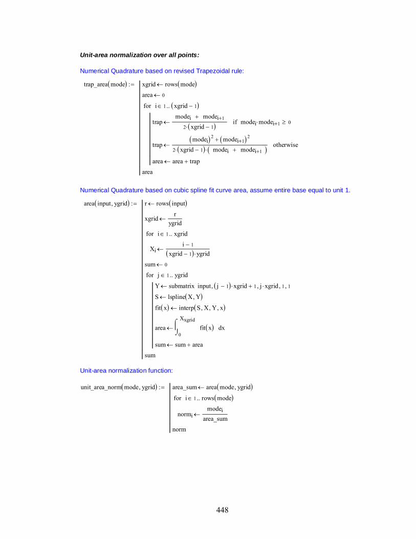
448
Unit-area normalization over all points:
Numerical Quadrature based on revised Trapezoidal rule:
trap_area mode xgrid rows mode
area 0
trapmodei modei 1
2 xgrid 1 modei modei 1 0if
trapmodei 2 modei 1 2
2 xgrid 1 modei modei 1 otherwise
area area trap
i 1 xgrid 1 for
area
Numerical Quadrature based on cubic spline fit curve area, assume entire base equal to unit 1.
area input ygrid r rows input
xgridr
ygrid
Xii 1
xgrid 1 ygrid
i 1 xgridfor
sum 0
Y submatrix input j 1 xgrid 1 j xgrid 1 1
S lspline X Y
fit x interp S X Y x
area0
Xxgrid
xfit x
d
sum sum area
j 1 ygridfor
sum
Unit-area normalization function:
unit_area_norm mode ygrid area_sum area mode ygrid
normimodei
area_sum
i 1 rows mode for
norm
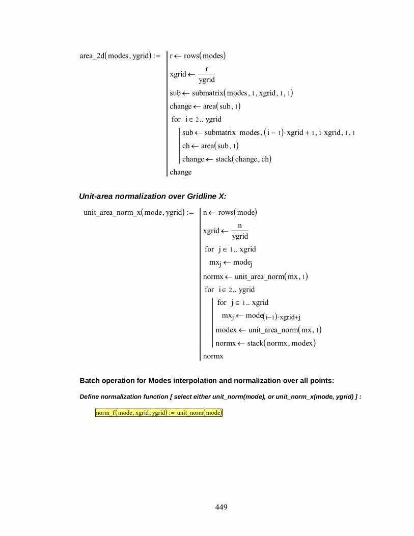
449
area_2d modes ygrid r rows modes
xgridr
ygrid
sub submatrix modes 1 xgrid 1 1
change area sub 1
sub submatrix modes i 1 xgrid 1 i xgrid 1 1
ch area sub 1
change stack change ch
i 2 ygridfor
change
Unit-area normalization over Gridline X:
unit_area_norm_x mode ygrid n rows mode
xgridn
ygrid
mxj modej
j 1 xgridfor
normx unit_area_norm mx 1
mxj mode i 1 xgrid j
j 1 xgridfor
modex unit_area_norm mx 1
normx stack normx modex
i 2 ygridfor
normx
Batch operation for Modes interpolation and normalization over all points:
Define normalization function [ select either unit_norm(mode), or unit_norm_x(mode, ygrid) ] :
norm_f mode xgrid ygrid unit_norm mode
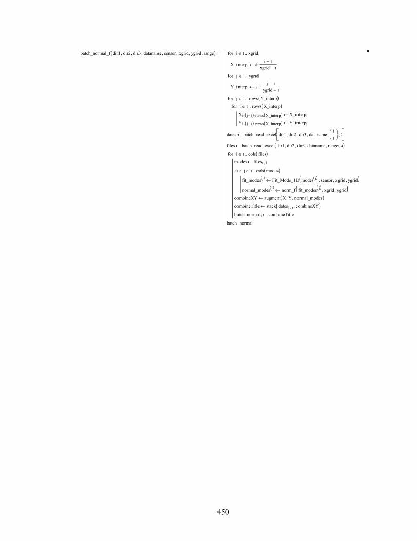
450
batch_normal_f dir1 dir2 dir3 dataname sensor xgrid ygrid range
X_interpi 8i 1
xgrid 1
i 1 xgridfor
Y_interpj 2.7j 1
ygrid 1
j 1 ygridfor
Xi j 1 rows X_interp X_interpi
Yi j 1 rows X_interp Y_interpj
i 1 rows X_interp for
j 1 rows Y_interp for
dates batch_read_excel dir1 dir2 dir3 dataname1
1
2
files batch_read_excel dir1 dir2 dir3 dataname range 4
modes files1 i
fit_modes j Fit_Mode_1D modes j sensor xgrid ygrid
normal_modes j norm_f fit_modes j xgrid ygrid
j 1 cols modes for
combineXY augment X Y normal_modes
combineTitle stack dates1 i combineXY
batch_normali combineTitle
i 1 cols files for
batch normal

451
Grid Points (Need ajusting according to requirements)
xgrid 41
ygrid 4
Acceleration Modes interpolation and normalization:
Input informations (need ajustment according different types):Testing dates, recorded sets and corresponding directories.
dir1 CWD
dir2 "Summary"
dir3 "\"
dataname1
12
3
4
5
6
7
"Mode 1_H_Acc_Dec 03 - July 19.xls""Mode 1_WN_Acc_Dec 03 - July 19.xls"
"Mode 2_H_Acc_Dec 03 - July 19.xls"
"Mode 2_WN_Acc_Dec 03 - July 19.xls"
"Mode 3_WN_Acc_Dec 03 - July 19.xls"
"Mode 4_WN_Acc_Dec 03 - July 19.xls"
"Mode 5_WN_Acc_Dec 03 - July 19.xls"
sensor "accl"
range 2 Notes: range equal to2 for accl(2, 28) for bottom strain(29, 55) for middle strain (56, 82) for top strain
Calculation and writing
batch_normal batch_normal_f dir1 dir2 dir3 dataname sensor xgrid ygrid range batch_normal_f
Notes for writing:Files have to be written one by one by changing file names and input matrix.
...\Mode 1_H.xls
batch_normal1
...\Mode 1_WN.xls
batch_normal2
...\Mode 2_H.xls
batch_normal3
...\Mode 2_WN.xls
batch_normal4
...\Mode 3_WN.xls
batch_normal5
...\Mode 4_WN.xls
batch_normal6
...\Mode 5_WN.xls
batch_normal7
Calculation and writing

452
M.5 Commonly Available VBDD Indicators
Change in Mode Shape
change_mode undamage damage damage undamage
change_mode_2d undamage damage change_mode undamage damage
Change in Mode Shape Curvature
Notes: using relative beam length 1, as a result, h=1/(n-1);using linear interpolation for end points at n=1 and n.
curvature modes n rows modes
curvi modesi 1 2 modesi modesi 1 n 1 2
i 2 n 1 for
curv1 0
curvn 0
curv
change_curvature undamage damage und curvature undamage
d curvature damage
d und
change_curvature_2d undamage damage r rows undamage
xgridr
ygrid
und submatrix undamage 1 xgrid 1 1
d submatrix damage 1 xgrid 1 1
change change_curvature und d
und submatrix undamage i 1 xgrid 1 i xgrid 1 1
d submatrix damage i 1 xgrid 1 i xgrid 1 1
ch change_curvature und d
change stack change ch
i 2 ygridfor
change

453
Change in Flexibility
Notes: assume w1 and w1d equal to 1, it could be to have positive influence on the result.
ω1 1 ω1d 1
change_flexibility undamage damage und1
ω12
undamage undamageT
d1
ω1d2
damage damageT
delta d und
n rows undamage
deli max delta i
i 1 nfor
del
ygrid 4 change this value if necessary
change_flexibility_2d undamage damage r rows undamage
xgridr
ygrid
und submatrix undamage 1 xgrid 1 1
d submatrix damage 1 xgrid 1 1
change change_flexibility und d
und submatrix undamage i 1 xgrid 1 i xgrid 1 1
d submatrix damage i 1 xgrid 1 i xgrid 1 1
ch change_flexibility und d
change stack change ch
i 2 ygridfor
change

454
Damage index mothod
Notes: assume the length of a segment from a to b equal to unit 1 for digital integration. Thisassumption has on influence on the results.
damage_index und d n rows und
sum1 0
sum2 0
sum1 sum1 undi 1 2 undi undi 1 2
sum2 sum2 di 1 2 di di 1 2
sub1i undi 1 2 undi undi 1 2
sub2i di 1 2 di di 1 2
i 2 n 1 for
cisub2i sum2 sum1
sub1i sum1 sum2
i 2 n 1 for
c1 0
b submatrix c 2 n 1 1 1
μ mean b
σ Stdev b
zibi μ
σ
i 1 n 2for
z stack 0 z 0
z
ygrid 4 change this value if necessary
damage_index_2d undamage damage r rows undamage
xgridr
ygrid
und submatrix undamage 1 xgrid 1 1
d submatrix damage 1 xgrid 1 1
change damage_index und d
und submatrix undamage i 1 xgrid 1 i xgrid 1 1
d submatrix damage i 1 xgrid 1 i xgrid 1 1
ch damage_index und d
change stack change ch
i 2 ygridfor
change
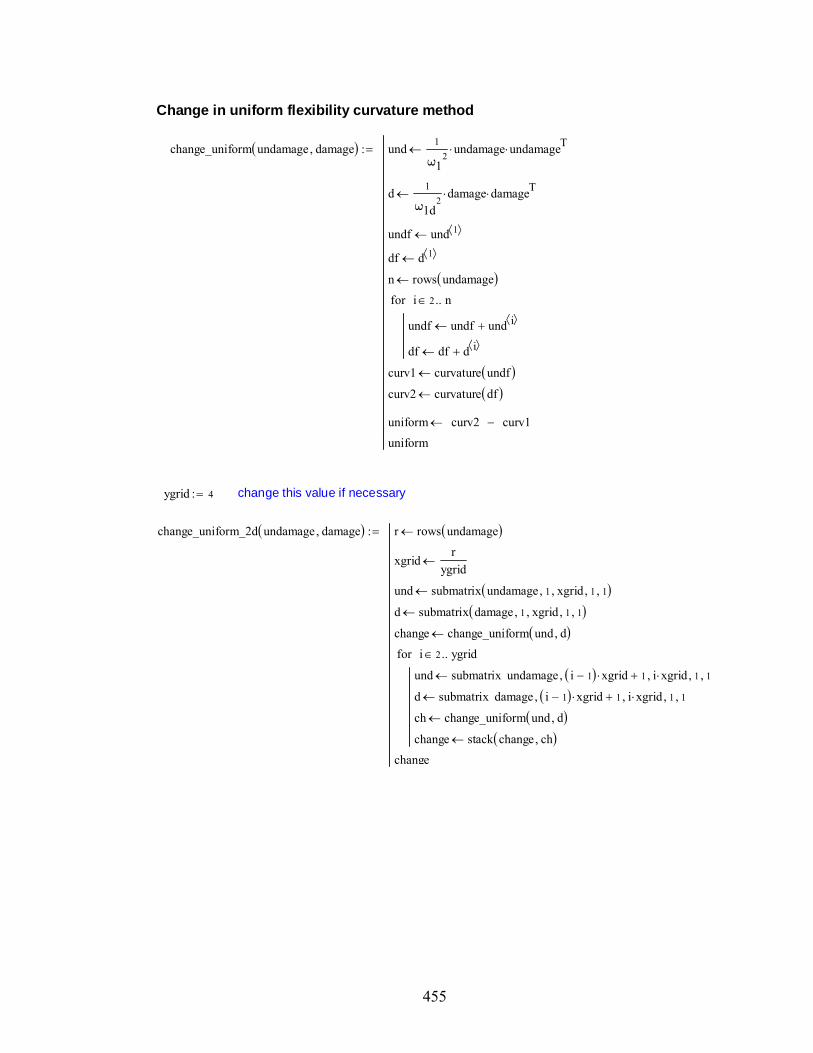
455
Change in uniform flexibility curvature method
change_uniform undamage damage und1
ω12
undamage undamageT
d1
ω1d2
damage damageT
undf und 1
df d 1
n rows undamage
undf undf und i
df df d i
i 2 nfor
curv1 curvature undf
curv2 curvature df
uniform curv2 curv1
uniform
ygrid 4 change this value if necessary
change_uniform_2d undamage damage r rows undamage
xgridr
ygrid
und submatrix undamage 1 xgrid 1 1
d submatrix damage 1 xgrid 1 1
change change_uniform und d
und submatrix undamage i 1 xgrid 1 i xgrid 1 1
d submatrix damage i 1 xgrid 1 i xgrid 1 1
ch change_uniform und d
change stack change ch
i 2 ygridfor
change
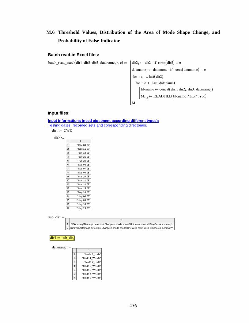
456
M.6 Threshold Values, Distribution of the Area of Mode Shape Change, and
Probability of False Indicator
Batch read-in Excel files:
batch_read_excel dir1 dir2 dir3 dataname r c dir21 dir2 rows dir2 0=if
dataname1 dataname rows dataname 0=if
filename concat dir1 dir2i dir3 datanamej
Mi j READFILE filename "Excel" r c
j 1 last dataname for
i 1 last dir2 for
M
Input files:
Input informations (need ajustment according different types):Testing dates, recorded sets and corresponding directories.
dir1 CWD
dir21
12
3
4
5
6
7
8
9
10
11
12
13
14
15
16
17
"Dec 03 07""Dec 11 07"
"Jan 18 08"
"Jan 21 08"
"Feb 25 08"
"Mar 03 08"
"Mar 07 08"
"Mar 08 08"
"Mar 10 08"
"Mar 11 08"
"Mar 14 08"
"Mar 15 08"
"May 26 08"
"July 04 08"
"July 05 08"
"July 18 08"
"July 19 08"
sub_dir1
12
"\Summary\Damage detection\Change in mode shape\Unit area norm all 9by4\area summary\"\Summary\Damage detection\Change in mode shape\Unit area norm xgrid 9by4\area summary\"
dir3 sub_dir1
dataname1
12
3
4
5
6
7
"Mode 1_H.xls""Mode 1_WN.xls"
"Mode 2_H.xls"
"Mode 2_WN.xls"
"Mode 3_WN.xls"
"Mode 4_WN.xls"
"Mode 5_WN.xls"
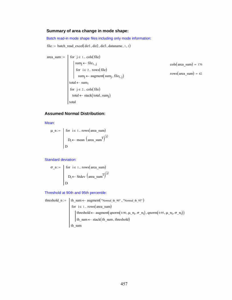
457
Summary of area change in mode shape:
Batch read-in mode shape files including only mode information:
file batch_read_excel dir1 dir2 dir3 dataname 1 1
area_sum
sumj file1 j
sumj augment sumj filei j
i 2 rows file for
j 1 cols file for
total sum1
total stack total sumj
j 2 cols file for
total
cols area_sum 170
rows area_sum 42
Assumed Normal Distribution:
Mean:
μ_n
Di mean area_sumT i
i 1 rows area_sum for
D
Standard deviation:
σ_n
Di Stdev area_sumT i
i 1 rows area_sum for
D
Threshold at 90th and 95th percentile:
threshold_n th_sum augment "Normal_th_90" "Normal_th_95"
threshold augment qnorm 0.90 μ_ni σ_ni qnorm 0.95 μ_ni σ_ni
th_sum stack th_sum threshold
i 1 rows area_sum for
th_sum

458
Assumed Log Normal Distribution:
Mean:
μ_Ln
Di mean ln area_sumT i
i 1 rows area_sum for
D
Standard deviation:
σ_Ln
Di Stdev ln area_sumT i
i 1 rows area_sum for
D
Threshold at 90th and 95th percentile:
threshold_Ln th_sum augment "Lognormal_th_90" "Lognormal_th_95"
threshold augment qlnorm 0.90 μ_Lni σ_Lni qlnorm 0.95 μ_Lni σ_Lni
th_sum stack th_sum threshold
i 1 rows area_sum for
th_sum
Actual distribution function:
cumulative distribution function:
cpdf input n rows input
sorted sort input
a 1
b 1
Xa sortedb
b b 1
Xa sortedb 1=while b nif
Yab
n
b b 1
a a 1
b nwhile
output augment X Y
output
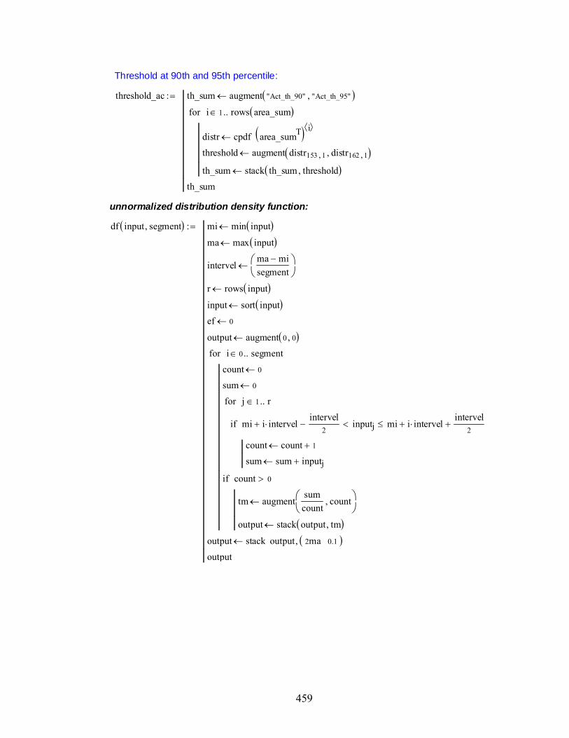
459
Threshold at 90th and 95th percentile:
threshold_ac th_sum augment "Act_th_90" "Act_th_95"
distr cpdf area_sumT i
threshold augment distr153 1 distr162 1
th_sum stack th_sum threshold
i 1 rows area_sum for
th_sum
unnormalized distribution density function:
df input segment mi min input
ma max input
intervelma misegment
r rows input
input sort input
ef 0
output augment 0 0
count 0
sum 0
count count 1
sum sum inputj
mi i intervelintervel
2 inputj mi i intervel
intervel2
if
j 1 rfor
tm augmentsum
countcount
output stack output tm
count 0if
i 0 segmentfor
output stack output 2ma 0.1
output

460
normalized distribution density function:
Area covered by the unnormalized density function:
density_area input X input 1
Y input 2
fit x linterp X Y x
armin X
max X xfit x
d
ar
Normalized density function:
normalized_df input segment output df input segment
n rows output
d_area density_area output
output 2 output 2
d_area
sub submatrix output 2 n 1 1 2
sub
Result summary:
result_sum input segment title1 augment "X" "Freq"
freq df input segment
title2 augment "Min" "Max"
min_max augment min input max input
title3 augment "X" "Density"
normalized normalized_df input segment
temp1 stack title1 freq
temp2 stack title2 min_max title3 normalized
output augment temp1 temp2
output
Result output:
tp 2 segment 5
...\tp_n5.xls
result_sum area_sumT tp segment

461
Testing procedures considered for plotting:
r 42
Area change and the corresponding probability:
th cpdf area_sumT r
90th Percentile: p90 153 actual_th95 thp90 1 0.26702273 actual_prob thp90 2 90 %
95th Percentile: p95 162 actual_th95 thp95 1 0.36631964 actual_prob thp95 2
x-axis of assumed distributions:
x th 1
Cumulative distribution function of Normal distribution:
norm t pnorm t μ_nr σ_nr
Cumulative distribution function of Lognormal distribution:
lgnorm t plnorm t μ_Lnr σ_Lnr
title augment "X" "Actual" "Normal" "Log-Norma
data augment x th 2 norm x lgnorm x
plot_data stack title data
...\cdp.xls
plot_data
0 0.2 0.4 0.6 0.8 10
0.2
0.4
0.6
0.8
1
Actual distributionNormal distribuitionLog-Normal distribuition
Cum
ulat
ive
prob
abil
ity
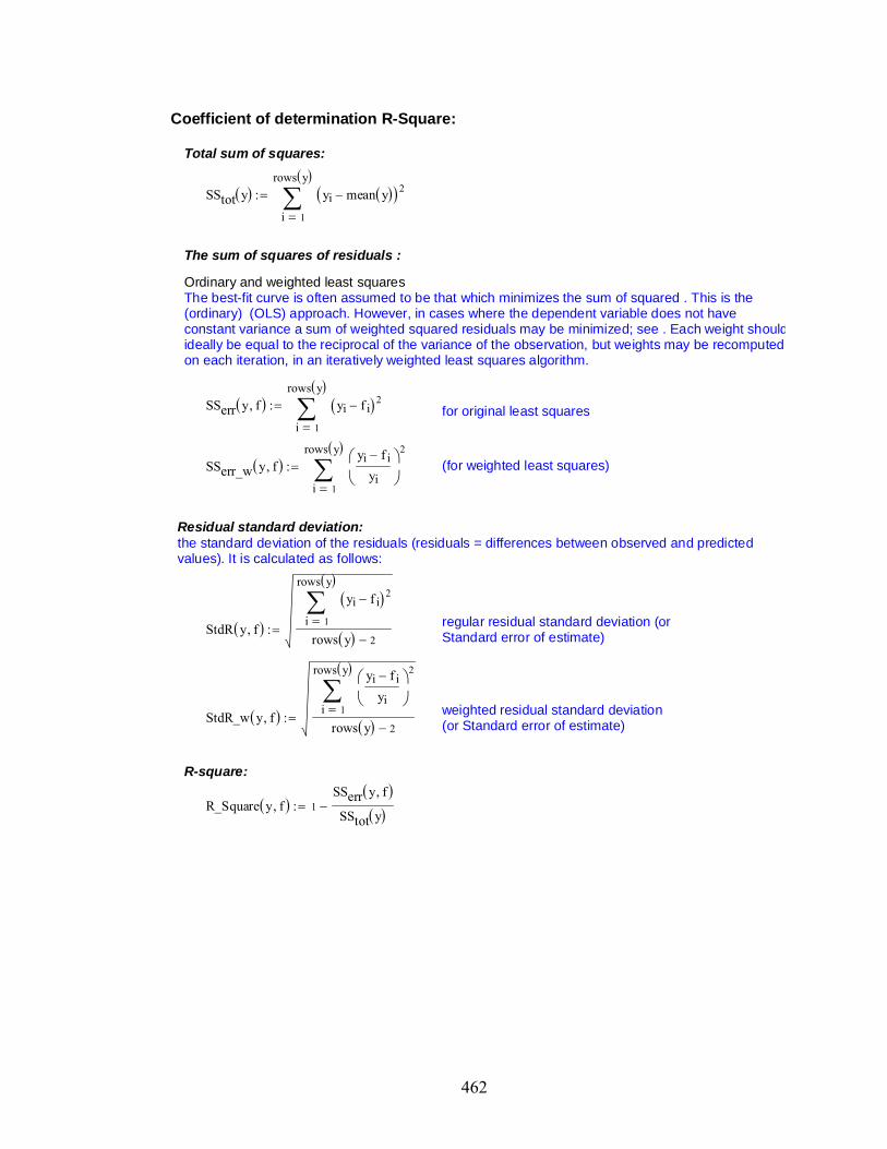
462
Coefficient of determination R-Square:
Total sum of squares:
SStot y 1
rows y
i
yi mean y 2
The sum of squares of residuals :
Ordinary and weighted least squaresThe best-fit curve is often assumed to be that which minimizes the sum of squared . This is the(ordinary) (OLS) approach. However, in cases where the dependent variable does not haveconstant variance a sum of weighted squared residuals may be minimized; see . Each weight shouldideally be equal to the reciprocal of the variance of the observation, but weights may be recomputedon each iteration, in an iteratively weighted least squares algorithm.
SSerr y f 1
rows y
i
yi f i 2
for original least squares
SSerr_w y f 1
rows y
i
yi f i
yi
2
(for weighted least squares)
Residual standard deviation: the standard deviation of the residuals (residuals = differences between observed and predictedvalues). It is calculated as follows:
regular residual standard deviation (orStandard error of estimate)
StdR y f 1
rows y
i
yi f i 2rows y 2
weighted residual standard deviation(or Standard error of estimate)
StdR_w y f 1
rows y
i
yi f i
yi
2
rows y 2
R-square:
R_Square y f 1SSerr y f SStot y

463
R-Square and standard errors based on Cumulative Dsitribution functions:
R_square_sum r_sum1 augment "R2_n" "SSerr_n" "StdR_n" "W_StdR_n"
r_sum2 augment "R2_lgn" "SSerr_lgn" "StdR_lgn" "W_StdR_lgn"
r_sum augment r_sum1 r_sum2
distr cpdf area_sumT r
X distr 1
Y distr 2
fnorm norm X
flgnorm lgnorm X
err1 SSerr Y fnorm
err2 SSerr Y flgnorm
stdr1 StdR Y fnorm
stdr2 StdR Y flgnorm
stdr1w StdR_w Y fnorm
stdr2w StdR_w Y flgnorm
R_sq1 R_Square Y fnorm
R_sq2 R_Square Y flgnorm
R_sq augment R_sq1 err1 stdr1 stdr1w R_sq2 err2 stdr2 stdr2w
r_sum stack r_sum R_sq
r 1 rows area_sum for
r sum

464
Results summary and output
title_mean stack "Normal Mean" μ_n title_std stack "Normal STD" σ_n
summary augment title_mean title_std threshold_ac threshold_Ln threshold_n R_square_sum
...\Threshold and standard errors.xls
summary
...\Area summary.xls
area_sum
Part of summary result:
summary
1 2 3 4 5
1
2
3
4
5
6
7
8
9
10
11
12
13
14
15
16
17
18
19
20
21
22
23
24
25
"Normal Mean" "Normal STD" "Act_th_90" "Act_th_95"gnormal_th_90"
0.00141697 0.00107138 0.0028835 0.0035926 0.00379488
0.00170129 0.0007275 0.00247491 0.00325764 0.0025683
0.00230243 0.00102508 0.00346954 0.00427984 0.00334363
0.00531793 0.00518958 0.00645764 0.01792083 0.00853913
0.00653018 0.00252703 0.00937213 0.01073326 0.00953098
0.00325612 0.00338555 0.00352712 0.01418534 0.00519156
0.00532558 0.00217632 0.00818653 0.00970211 0.00828951
0.02532351 0.00607721 0.0320982 0.0361508 0.03396546
0.03776464 0.0083548 0.04883533 0.0517702 0.04872723
0.06866162 0.01440428 0.0875684 0.09297759 0.08910203
0.09652527 0.02258459 0.12357489 0.13633643 0.12762836
0.04281005 0.01043486 0.05725089 0.06163811 0.05619855
0.01766498 0.01665966 0.03900192 0.05093513 0.05178742
0.00843858 0.00675301 0.01749179 0.02030148 0.0161647
0.01137913 0.00836968 0.02289542 0.02911297 0.0208864
0.02053768 0.01473792 0.04619171 0.04835126 0.0381196
0.02717711 0.0172801 0.05149765 0.05946237 0.04809481
0.02446662 0.03318087 0.05625041 0.0648315 0.04789721
0.04950986 0.0670098 0.07436397 0.10738581 0.08777878
0.2309657 0.14998371 0.45593362 0.58666981 0.42208666
0.24915725 0.13775665 0.43078865 0.51134156 0.42956772
0.377285 0.16838072 0.60196522 0.67746299 0.60732784
0.46083625 0.16860379 0.73404504 0.77510704 0.6983895
0.30174896 0.1297328 0.47399727 0.55040961 ...

465
Summary of area change in mode shape due to damage:
Input informations (need ajustment according different types):Testing dates, recorded sets and corresponding directories.
dir1 concat CWD "Summary\Damage detection\Area of mode shape change\"
dir21
1
2
3
4
5
6
"Accl"
"B Strain"
"M Strain"
"T Strain"
"B_M curvature Strain"
"Best fit curvature Strain"
dir3 "\"
dataname1
12
3
4
5
6
7
"Mode 1_H.xls""Mode 1_WN.xls"
"Mode 2_H.xls"
"Mode 2_WN.xls"
"Mode 3_WN.xls"
"Mode 4_WN.xls"
"Mode 5_WN.xls"
Batch read-in Mean and Standard Deviation of Normal distribution:
mean_file batch_read_excel dir1 dir2 dir3 dataname28
28
2
stdev_file batch_read_excel dir1 dir2 dir3 dataname29
29
2
stack_column file n cols file
output file 1
output stack output file i
i 2 nfor
output
Mean values for all damage cases and all test protocols
mean_d stack_column mean_file
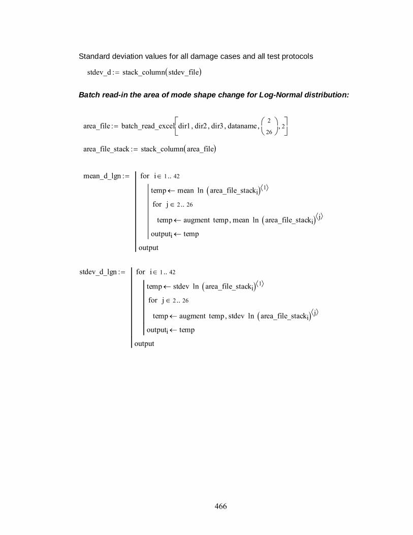
466
Standard deviation values for all damage cases and all test protocols
stdev_d stack_column stdev_file
Batch read-in the area of mode shape change for Log-Normal distribution:
area_file batch_read_excel dir1 dir2 dir3 dataname2
26
2
area_file_stack stack_column area_file
mean_d_lgn
temp mean ln area_file_stacki 1
temp augment temp mean ln area_file_stacki j
j 2 26for
outputi temp
i 1 42for
output
stdev_d_lgn
temp stdev ln area_file_stacki 1
temp augment temp stdev ln area_file_stacki j
j 2 26for
outputi temp
i 1 42for
output

467
Define probability that there has been a change in condition by comparing twogroups (undamaged and damaged groups):
Statistic values of undamaged group based on normal distribution:
mean_und μ_n
stdev_und σ_n
Plots of density function :
Original test protocols: tp 1
Damage case: dc 26
Segment of intervel for actual density function: segment 5
Plot axias range:
xL 0 xU 0.01
yL 0 yU 800 y 0 yU
Plots of the actual, Normal and Log-Normal density function of undamagedgroups:
Plots of normal density function of both undamaged and damaged samplegroups:
Plot axias range:
xL 0.01 xU 0.1
yL 0 yU 800 y 0 yU

468
Normal distribution:
0.01 0 0.01 0.02 0.03 0.04 0.05 0.06 0.07 0.08 0.09 0.10
200
400
600
800
Distribution of undamaged groupDistribution of damaged group90th percentile of undamaged group95th percentile of undamaged group
The area of mode shape change
Dis
trib
utio
n de
nsit
y
Log-Normal distribution:
0.01 0 0.01 0.02 0.03 0.04 0.05 0.06 0.07 0.08 0.09 0.10
200
400
600
800
Distribution of undamaged groupDistribution of damaged group90th percentile of undamaged group95th percentile of undamaged group
The area of mode shape change
Dis
trib
utio
n de
nsit
y

469
Probability that the value from the damaged group does not exceed that from undamagedgroup (i.e. the probability that there is no change in condition):
Normal distribution:
Pf m1 std1 m2 std2
∞
∞
xdnorm x m1 std1 ∞
x
tdnorm t m2 std2
d
d
prob_sum prob "TP"
prob augment prob j
j 1 26for
tp i
tp augment tp Pf mean_undi stdev_undi mean_di 1 j
stdev_di 1 j
j 1 26for
prob stack prob tp
i 1 42for
prob
Result output...\Probability summary.xls
prob_sum
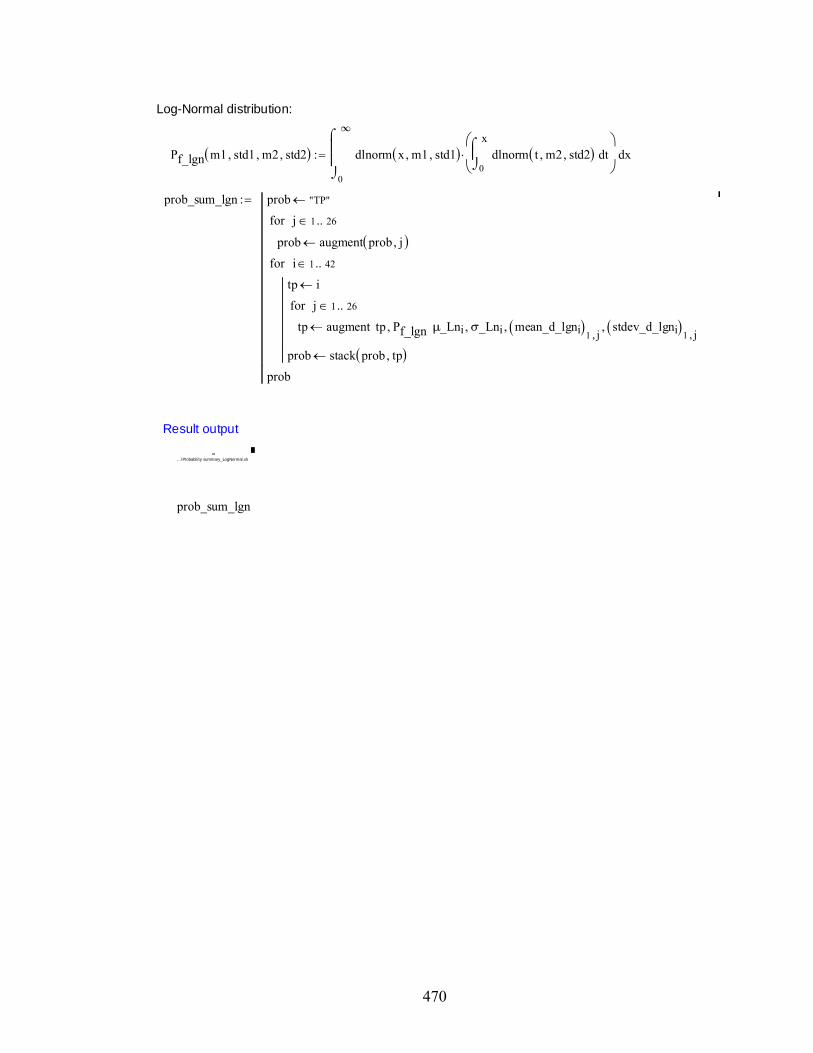
470
Log-Normal distribution:
Pf_lgn m1 std1 m2 std2 0
∞
xdlnorm x m1 std1 0
x
tdlnorm t m2 std2
d
d
prob_sum_lgn prob "TP"
prob augment prob j
j 1 26for
tp i
tp augment tp Pf_lgn μ_Lni σ_Lni mean_d_lgni 1 j
stdev_d_lgni 1 j
j 1 26for
prob stack prob tp
i 1 42for
prob
Result output
...\Probability summary_LogNormal.xls
prob_sum_lgn

471
R-Square and standard errors based on Probability Density functions:
R_square_sum_df r_sum1 augment "R2_n" "SSerr_n" "StdR_n" "W_StdR_n"
r_sum2 augment "R2_lgn" "SSerr_lgn" "StdR_lgn" "W_StdR_lgn"
r_sum augment r_sum1 r_sum2
distr normalized_df area_sumT r 5
X distr 1
Y distr 2
fnorm norm X
flgnorm lgnorm X
err1 SSerr Y fnorm
err2 SSerr Y flgnorm
stdr1 StdR Y fnorm
stdr2 StdR Y flgnorm
stdr1w StdR_w Y fnorm
stdr2w StdR_w Y flgnorm
R_sq1 R_Square Y fnorm
R_sq2 R_Square Y flgnorm
R_sq augment R_sq1 err1 stdr1 stdr1w R_sq2 err2 stdr2 stdr2w
r_sum stack r_sum R_sq
r 1 rows area_sum for
r_sum
summary_df augment title_mean title_std threshold_ac threshold_Ln threshold_n R_square_sum_df
...\Threshold and standard errors based on density function.xls
summary_df
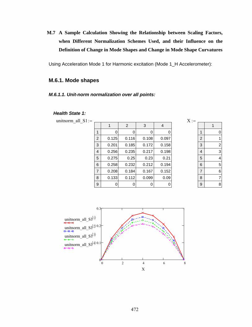
472
M.7 A Sample Calculation Showing the Relationship between Scaling Factors,
when Different Normalization Schemes Used, and their Influence on the
Definition of Change in Mode Shapes and Change in Mode Shape Curvatures
Using Acceleration Mode 1 for Harmonic excitation (Mode 1_H Accelerometer):
M.6.1. Mode shapes
M.6.1.1. Unit-norm normalization over all points:
Health State 1:
unitnorm_all_S11 2 3 4
1
2
3
4
5
6
7
8
9
0 0 0 0
0.125 0.116 0.108 0.097
0.201 0.185 0.172 0.158
0.256 0.235 0.217 0.198
0.275 0.25 0.23 0.21
0.258 0.232 0.212 0.194
0.208 0.184 0.167 0.152
0.133 0.112 0.099 0.09
0 0 0 0
X1
1
2
3
4
5
6
7
8
9
0
1
2
3
4
5
6
7
8
0 2 4 6 80
0.1
0.2
0.3
unitnorm_all_S1 1
unitnorm_all_S1 2
unitnorm_all_S1 3
unitnorm_all_S1 4
X
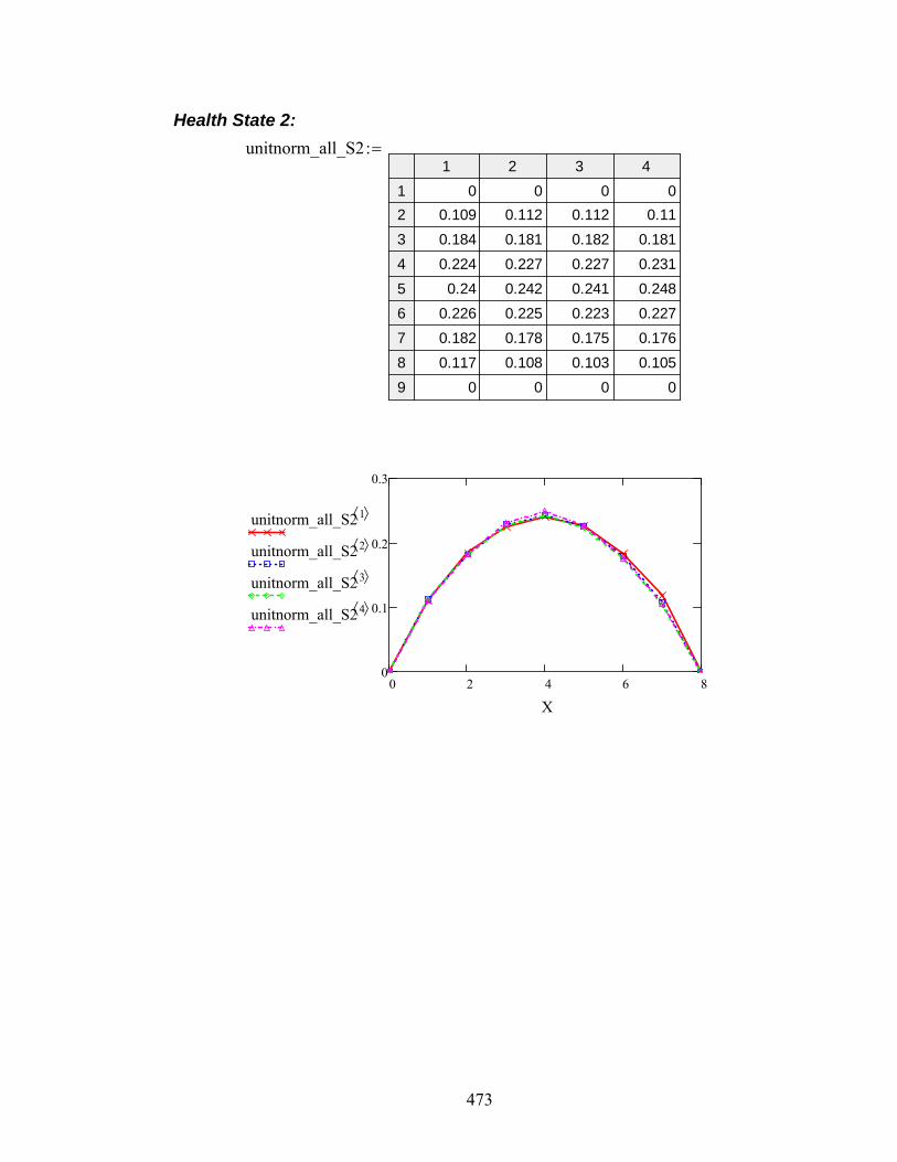
473
Health State 2:
unitnorm_all_S21 2 3 4
1
2
3
4
5
6
7
8
9
0 0 0 0
0.109 0.112 0.112 0.11
0.184 0.181 0.182 0.181
0.224 0.227 0.227 0.231
0.24 0.242 0.241 0.248
0.226 0.225 0.223 0.227
0.182 0.178 0.175 0.176
0.117 0.108 0.103 0.105
0 0 0 0
0 2 4 6 80
0.1
0.2
0.3
unitnorm_all_S21
unitnorm_all_S22
unitnorm_all_S23
unitnorm_all_S24
X
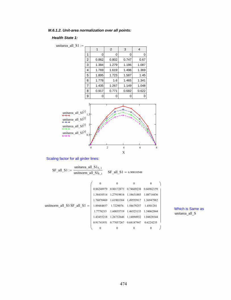
474
M.6.1.2. Unit-area normalization over all points:
Health State 1:
unitarea_all_S11 2 3 4
1
2
3
4
5
6
7
8
9
0 0 0 0
0.862 0.802 0.747 0.67
1.384 1.279 1.186 1.087
1.769 1.619 1.496 1.369
1.895 1.723 1.587 1.45
1.778 1.6 1.465 1.341
1.435 1.267 1.149 1.048
0.917 0.771 0.682 0.622
0 0 0 0
0 2 4 6 80
0.5
1
1.5
2
unitarea_all_S11
unitarea_all_S12
unitarea_all_S13
unitarea_all_S14
X
Scaling factor for all girder lines:
SF_all_S1unitarea_all_S15 1unitnorm_all_S15 1
SF_all_S1 6.90010548
unitnorm_all_S1 SF_all_S1
0
0.86248979
1.38410514
1.76870469
1.89484857
1.7776213
1.43455218
0.91741931
0
0
0.80172873
1.27919814
1.61903384
1.7229076
1.60035719
1.26732646
0.77057267
0
0
0.74669238
1.18631885
1.49555917
1.58679257
1.46523133
1.14894932
0.68187947
0
0
0.66962159
1.08714436
1.36947982
1.4501281
1.34062844
1.04828544
0.6224235
0
Which is Same asunitarea_all_S

475
Health State 2:
unitarea_all_S21 2 3 4
1
2
3
4
5
6
7
8
9
0 0 0 0
0.75 0.769 0.769 0.755
1.261 1.247 1.248 1.243
1.541 1.56 1.559 1.584
1.651 1.661 1.656 1.702
1.55 1.545 1.531 1.557
1.252 1.224 1.199 1.211
0.802 0.744 0.71 0.718
0 0 0 0
0 2 4 6 80
0.5
1
1.5
2
unitarea_all_S2 1
unitarea_all_S2 2
unitarea_all_S2 3
unitarea_all_S2 4
X
Scaling factor for all girder lines:
SF_all_S2unitarea_all_S25 1unitnorm_all_S25 1
SF_all_S2 6.86869647
unitnorm_all_S2 SF_all_S2
0
0.75042142
1.26112417
1.5407054
1.65112044
1.55013385
1.25181003
0.80246555
0
0
0.76887012
1.24650487
1.56017871
1.66089321
1.54464069
1.22446615
0.74431212
0
0
0.76868315
1.24752654
1.55866044
1.6564796
1.53073812
1.19881889
0.71043217
0
0
0.75536814
1.24330368
1.58356469
1.70229927
1.55706157
1.21111523
0.71830179
0
Which is same as unitarea_all_S2
Scaling factors are different for two damage cases:
SF_all_S1
SF_all_S21.00457278

476
M.6.1.3. Unit-area normalization along each girder line:
Health State 1:
unitarea_xgrid_S11 2 3 4
1
2
3
4
5
6
7
8
9
0 0 0 0
0.687 0.708 0.719 0.706
1.103 1.129 1.142 1.146
1.409 1.429 1.44 1.444
1.51 1.521 1.527 1.529
1.416 1.413 1.41 1.413
1.143 1.119 1.106 1.105
0.731 0.68 0.656 0.656
0 0 0 0
0 2 4 6 80
0.5
1
1.5
2
unitarea_xgrid_S11
unitarea_xgrid_S12
unitarea_xgrid_S13
unitarea_xgrid_S14
X
Scaling factors are different for each girder line:
Girder Line 1: SF_xgrid_G1_S1unitarea_xgrid_S15 1unitnorm_all_S15 1
SF_xgrid_G1_S1 5.49823387
Girder Line 2: SF_xgrid_G2_S1unitarea_xgrid_S15 2unitnorm_all_S15 2
SF_xgrid_G2_S1 6.09205214
Girder Line 3: SF_xgrid_G3_S1unitarea_xgrid_S15 3unitnorm_all_S15 3
SF_xgrid_G3_S1 6.64156345
Girder Line 4: SF_xgrid_G4_S1unitarea_xgrid_S15 4unitnorm_all_S15 4
SF_xgrid_G4_S1 7.27503222

477
Normalized mode shape:
G1 unitnorm_all_S1 1 SF_xgrid_G1_S1 G2 unitnorm_all_S1 2 SF_xgrid_G2_S1
G3 unitnorm_all_S1 3 SF_xgrid_G3_S1 G4 unitnorm_all_S1 4 SF_xgrid_G4_S1
Normalized_unitarea_xgrid_S1 augment G1 G2 G3 G4( )
Normalized_unitarea_xgrid_S1
0
0.68726059
1.10290107
1.4093628
1.50987845
1.41646786
1.14309896
0.73103026
0
0
0.70784038
1.12939459
1.42943301
1.52114239
1.41294354
1.11891317
0.68033292
0
0
0.71871434
1.14186833
1.43952164
1.52733658
1.41033015
1.10589901
0.65632993
0
0
0.7060064
1.14621585
1.44389239
1.52892281
1.41347334
1.10524548
0.65624374
0
Same as unitarea_xgrid_S1
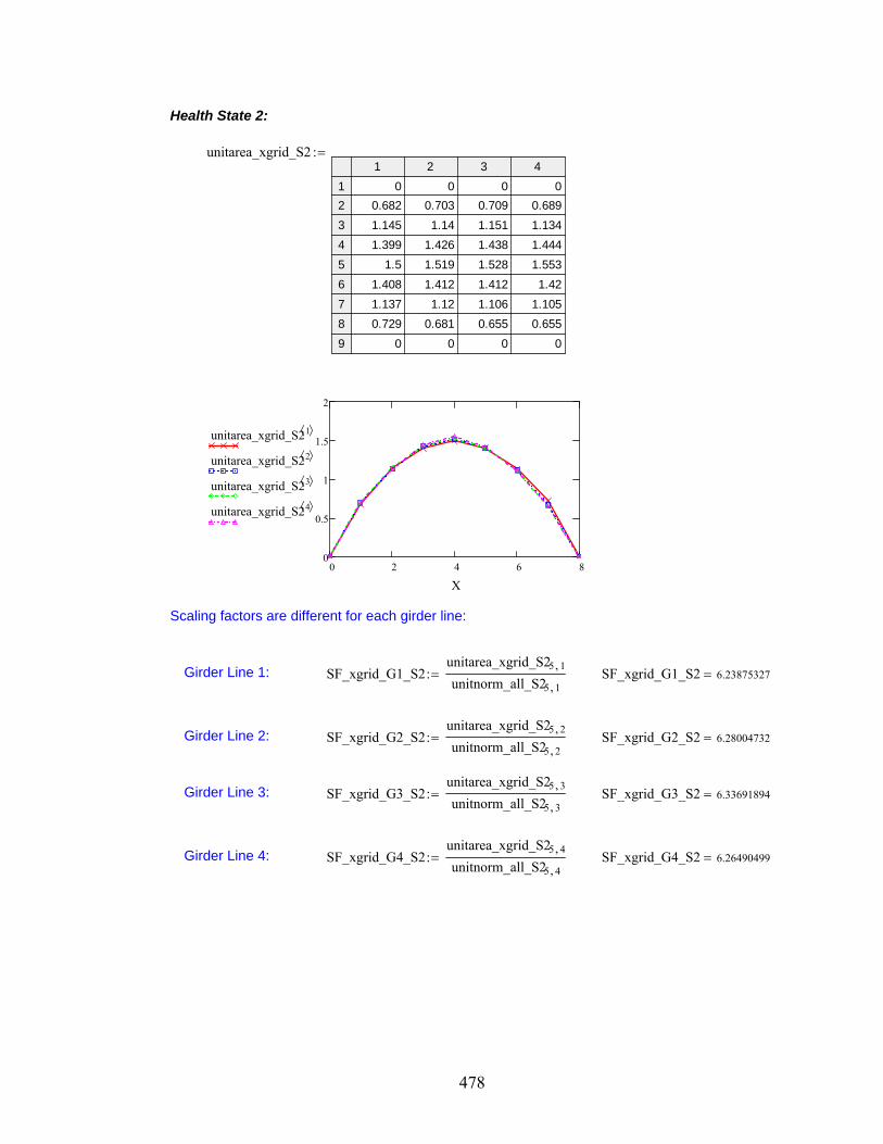
478
Health State 2:
unitarea_xgrid_S21 2 3 4
1
2
3
4
5
6
7
8
9
0 0 0 0
0.682 0.703 0.709 0.689
1.145 1.14 1.151 1.134
1.399 1.426 1.438 1.444
1.5 1.519 1.528 1.553
1.408 1.412 1.412 1.42
1.137 1.12 1.106 1.105
0.729 0.681 0.655 0.655
0 0 0 0
0 2 4 6 80
0.5
1
1.5
2
unitarea_xgrid_S21
unitarea_xgrid_S22
unitarea_xgrid_S23
unitarea_xgrid_S24
X
Scaling factors are different for each girder line:
Girder Line 1: SF_xgrid_G1_S2unitarea_xgrid_S25 1unitnorm_all_S25 1
SF_xgrid_G1_S2 6.23875327
Girder Line 2: SF_xgrid_G2_S2unitarea_xgrid_S25 2unitnorm_all_S25 2
SF_xgrid_G2_S2 6.28004732
Girder Line 3: SF_xgrid_G3_S2unitarea_xgrid_S25 3unitnorm_all_S25 3
SF_xgrid_G3_S2 6.33691894
Girder Line 4: SF_xgrid_G4_S2unitarea_xgrid_S25 4unitnorm_all_S25 4
SF_xgrid_G4_S2 6.26490499
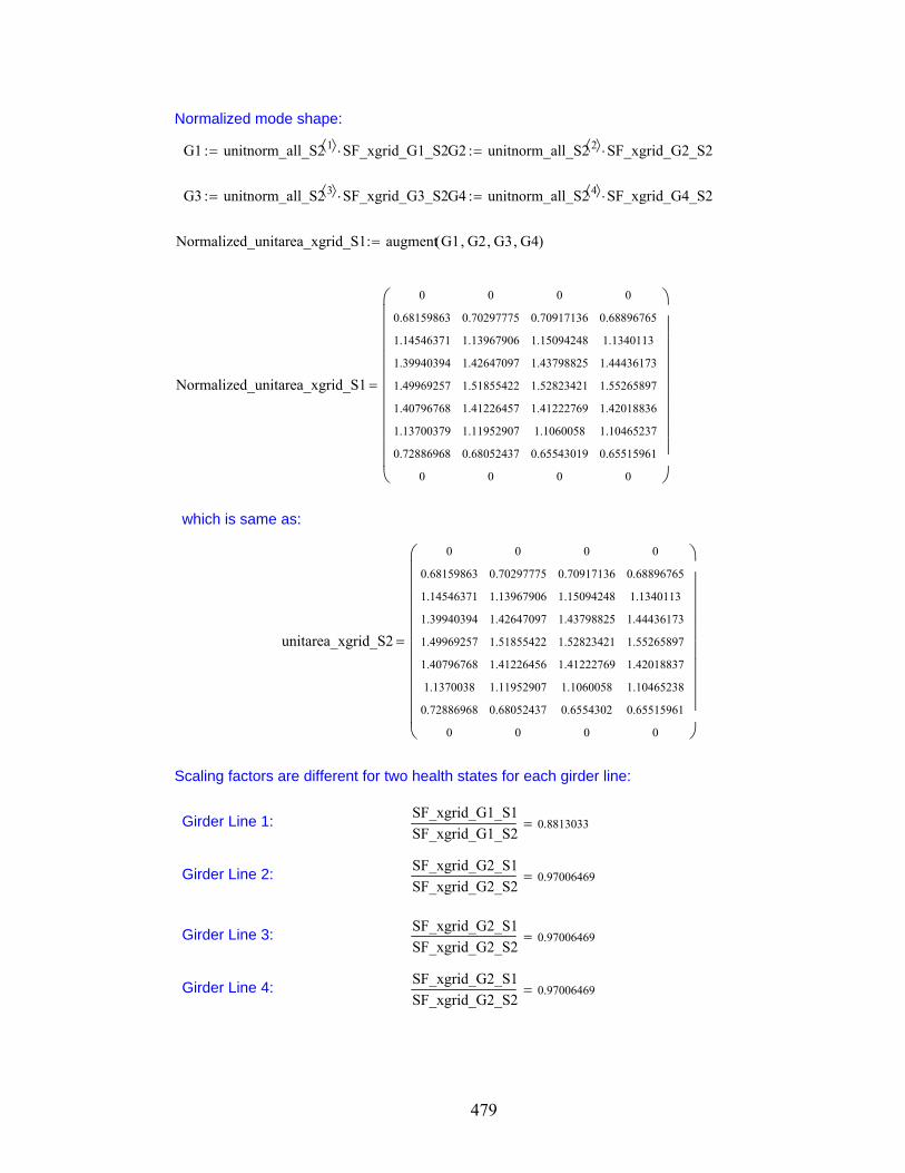
479
Normalized mode shape:
G1 unitnorm_all_S2 1 SF_xgrid_G1_S2 G2 unitnorm_all_S2 2 SF_xgrid_G2_S2
G3 unitnorm_all_S2 3 SF_xgrid_G3_S2 G4 unitnorm_all_S2 4 SF_xgrid_G4_S2
Normalized_unitarea_xgrid_S1 augment G1 G2 G3 G4( )
Normalized_unitarea_xgrid_S1
0
0.68159863
1.14546371
1.39940394
1.49969257
1.40796768
1.13700379
0.72886968
0
0
0.70297775
1.13967906
1.42647097
1.51855422
1.41226457
1.11952907
0.68052437
0
0
0.70917136
1.15094248
1.43798825
1.52823421
1.41222769
1.1060058
0.65543019
0
0
0.68896765
1.1340113
1.44436173
1.55265897
1.42018836
1.10465237
0.65515961
0
which is same as:
unitarea_xgrid_S2
0
0.68159863
1.14546371
1.39940394
1.49969257
1.40796768
1.1370038
0.72886968
0
0
0.70297775
1.13967906
1.42647097
1.51855422
1.41226456
1.11952907
0.68052437
0
0
0.70917136
1.15094248
1.43798825
1.52823421
1.41222769
1.1060058
0.6554302
0
0
0.68896765
1.1340113
1.44436173
1.55265897
1.42018837
1.10465238
0.65515961
0
Scaling factors are different for two health states for each girder line:
Girder Line 1:SF_xgrid_G1_S1
SF_xgrid_G1_S20.8813033
Girder Line 2:SF_xgrid_G2_S1
SF_xgrid_G2_S20.97006469
Girder Line 3:SF_xgrid_G2_S1
SF_xgrid_G2_S20.97006469
Girder Line 4:SF_xgrid_G2_S1
SF_xgrid_G2_S20.97006469

480
M.6.2 . Change in Mode Shape.
M.6.2.1. Unit-area normalization over all points:
ch_m_areanorm_all unitarea_all_S2 unitarea_all_S1
ch_m_areanorm_all
0
0.112068360.122980970.227999280.243728130.227487450.182742140.11495376
0
0
0.032858610.032693280.058855130.062014390.055716510.042860310.02626055
0
0
0.02199078
0.06120769
0.06310126
0.06968703
0.06550679
0.04986957
0.0285527
0
0
0.08574655
0.15615932
0.21408486
0.25217116
0.21643312
0.16282979
0.09587829
0
0 2 4 6 8
0.3
0.2
0.1
0.1
0.2
0.3
ch_m_areanorm_all 1
ch_m_areanorm_all 2
ch_m_areanorm_all 3
ch_m_areanorm_all 4
X

481
M.6.2.2. Unit-area normalization along each girder line:
ch_m_areanorm_xgrid unitarea_xgrid_S2 unitarea_xgrid_S1
ch_m_areanorm_xgrid
0
0.005661960.04256263
0.009958870.010185890.008500180.006095160.00216059
0
0
0.004862630.01028447
0.002962040.002588180.000678980.0006159
0.00019145
0
0
0.009542980.00907415
0.001533390.00089763
0.00189753
0.00010679
0.000899730
0
0.017038750.01220454
0.00046934
0.02373616
0.00671503
0.00059310.00108413
0
0 2 4 6 8
0.02
0.02
0.04
0.06
ch_m_areanorm_xgrid1
ch_m_areanorm_xgrid2
ch_m_areanorm_xgrid 3
ch_m_areanorm_xgrid4
X

482
M.6.3. Mode Shape Curvature and Change in Mode Shape Curvature
M.6.3.1. Mode shape curvature
M.6.3.1.1. Unit-norm normalization over all points:
Health State 1:
modeshape unitnorm_all_S1
curv1 curvature modeshape 1 curv2 curvature modeshape 2
curv3 curvature modeshape 3 curv4 curvature modeshape 4
curv augment curv1 curv2 curv3 curv4( )
curv
0
3.161685571.270851782.397233282.257321152.094732931.614479683.71274502
0
0
3.007576771.276583042.188598912.100134211.952251331.518567492.53973056
0
0
2.848103941.209360322.022062341.973717181.806078021.398590531.99240659
0
0
2.338272191.25389211.870693061.763664061.695912321.23841761.82315187
0
0 2 4 6 8
4
3
2
1curv 1
curv 2
curv 3
curv 4
X
curv_unitnorm_all_S1 curv
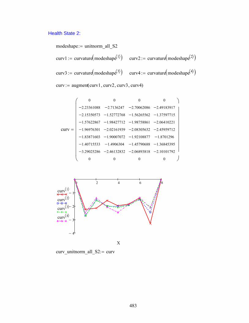
483
Health State 2:
modeshape unitnorm_all_S2
curv1 curvature modeshape 1 curv2 curvature modeshape 2
curv3 curvature modeshape 3 curv4 curvature modeshape 4
curv augment curv1 curv2 curv3 curv4( )
curv
0
2.233610882.153505731.576228671.969763011.838716031.407155333.29025286
0
0
2.71362471.527727681.984277122.021619391.900070721.4906304
2.461328320
0
2.700620861.562655621.987588612.083056321.921088771.457906882.06893818
0
0
2.491839171.375977152.064102212.459597121.8701296
1.368453952.10101792
0
0 2 4 6 8
4
3
2
1curv 1
curv 2
curv 3
curv 4
X
curv_unitnorm_all_S2 curv
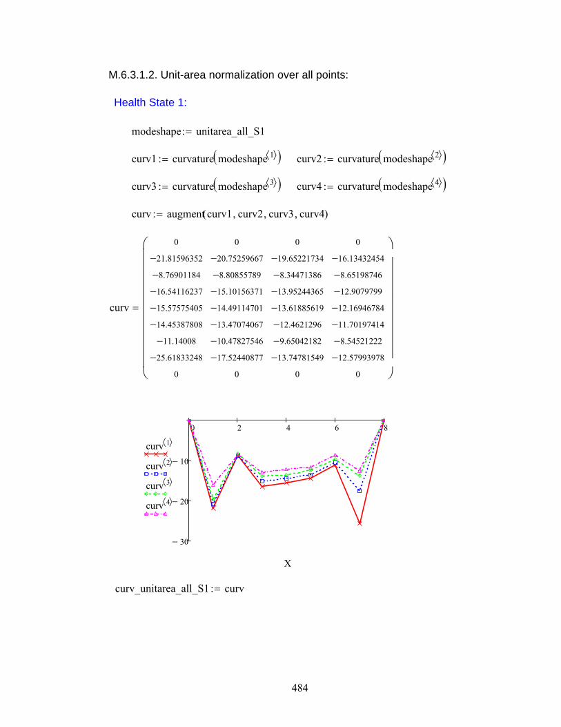
484
M.6.3.1.2. Unit-area normalization over all points:
Health State 1:
modeshape unitarea_all_S1
curv1 curvature modeshape 1 curv2 curvature modeshape 2
curv3 curvature modeshape 3 curv4 curvature modeshape 4
curv augment curv1 curv2 curv3 curv4( )
curv
0
21.815963528.76901184
16.5411623715.5757540514.45387808
11.1400825.61833248
0
0
20.752596678.80855789
15.1015637114.4911470113.4707406710.4782754617.52440877
0
0
19.652217348.34471386
13.9524436513.6188561912.46212969.65042182
13.747815490
0
16.134324548.6519874612.9079799
12.1694678411.701974148.54521222
12.579939780
0 2 4 6 8
30
20
10curv 1
curv 2
curv 3
curv 4
X
curv_unitarea_all_S1 curv

485
Health State 2:
modeshape unitarea_all_S2
curv1 curvature modeshape 1 curv2 curvature modeshape 2
curv3 curvature modeshape 3 curv4 curvature modeshape 4
curv augment curv1 curv2 curv3 curv4( )
curv
0
15.3419951414.791776910.8266367413.5297038712.62958246
9.665323222.59974778
0
0
18.6390649610.4934971513.629397713.8858899813.0510088310.2386873616.90611776
0
0
18.5497452810.733407313.6521425314.3078816613.1953757410.0139193614.21090886
0
0
17.115686539.4511700514.1776911416.8942259212.84535279.3994949114.4312544
0
which is same as
SF_all_S2 curv_unitnorm_all_S2
0
15.3419951614.7917771910.8266363113.5297042212.629582329.6653228322.59974823
0
0
18.6390644210.4934977213.6293972513.8858899813.0510090410.2386877616.90611714
0
0
18.5497449910.7334071113.6521428514.3078815913.1953756410.0139198414.21090834
0
0
17.115686899.4511694
14.1776915516.8942260512.845352589.39949483
14.431254370
0 2 4 6 8
30
20
10curv 1
curv 2
curv 3
curv 4
X
curv_unitarea_all_S2 curv

486
M.6.3.1.3. Unit-area normalization along individual girder lines:
Health State 1:
modeshape unitarea_xgrid_S1
curv1 curvature modeshape 1 curv2 curvature modeshape 2
curv3 curvature modeshape 3 curv4 curvature modeshape 4
curv augment curv1 curv2 curv3 curv4( )
curv
0
17.383686216.98744083
13.1805489912.4112796811.517331398.87678688
20.413540480
0
18.32231437.77701062
13.3330590112.7941266611.89321734
9.25119215.47217094
0
0
18.915862728.03204339
13.4296555513.1085673611.995182539.28882739
13.232694660
0
17.011005189.12210522
13.6093526412.8307127
12.337816969.00952813
13.263488060
0 2 4 6 8
30
20
10curv 1
curv 2
curv 3
curv 4
X

487
Verification:
c1 SF_xgrid_G1_S1 curv_unitnorm_all_S1 1
c2 SF_xgrid_G2_S1 curv_unitnorm_all_S1 2
c3 SF_xgrid_G3_S1 curv_unitnorm_all_S1 3
c4 SF_xgrid_G4_S1 curv_unitnorm_all_S1 4
curv_normalized augment c1 c2 c3 c4
curv_normalized
0
17.383686676.9874402713.1805492112.4112796111.517331538.8767868520.41354043
0
0
18.32231457.7770104413.3330586912.794127111.893216899.2511923215.472171
0
0
18.9158638.032043313.429655313.1085679111.995181749.2888277313.2326948
0
0
17.011005549.1221054
13.6093522612.830712912.337816789.0095279513.26348862
0
which is same as above matrix.
curv_unitarea_xgrid_S1 curv
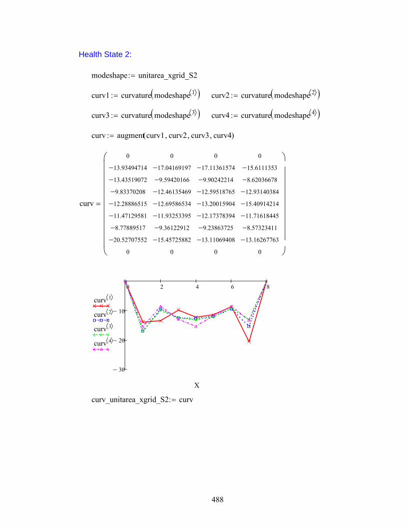
488
Health State 2:
modeshape unitarea_xgrid_S2
curv1 curvature modeshape 1 curv2 curvature modeshape 2
curv3 curvature modeshape 3 curv4 curvature modeshape 4
curv augment curv1 curv2 curv3 curv4( )
curv
0
13.9349471413.435190729.8337020812.2888651511.471295818.7788951720.52707552
0
0
17.041691979.5942016612.4613546912.6958653411.932533959.3612291215.45725882
0
0
17.113615749.9024221412.5951876513.2001590412.173783949.2386372513.11069408
0
0
15.61113538.6203667812.9314038415.4091421411.716184458.5732341113.16267763
0
0 2 4 6 8
30
20
10curv 1
curv 2
curv 3
curv 4
X
curv_unitarea_xgrid_S2 curv

489
Verification:
c1 SF_xgrid_G1_S2 curv_unitnorm_all_S21
c2 SF_xgrid_G2_S2 curv_unitnorm_all_S22
c3 SF_xgrid_G3_S2 curv_unitnorm_all_S23
c4 SF_xgrid_G4_S2 curv_unitnorm_all_S24
curv_normalized augment c1 c2 c3 c4( )
curv_normalized
0
13.9349471913.435190919.83370179
12.2888654211.471295678.77889491
20.527075830
0
17.041691569.59420213
12.4613542212.6958654511.932534049.36122945
15.457258330
0
17.113615499.90242196
12.5951878913.2001590412.173783799.2386377113.1106935
0
0
15.611135658.62036613
12.9314042315.4091422811.71618427
8.57323413.16267766
0
which is same as above matrix.
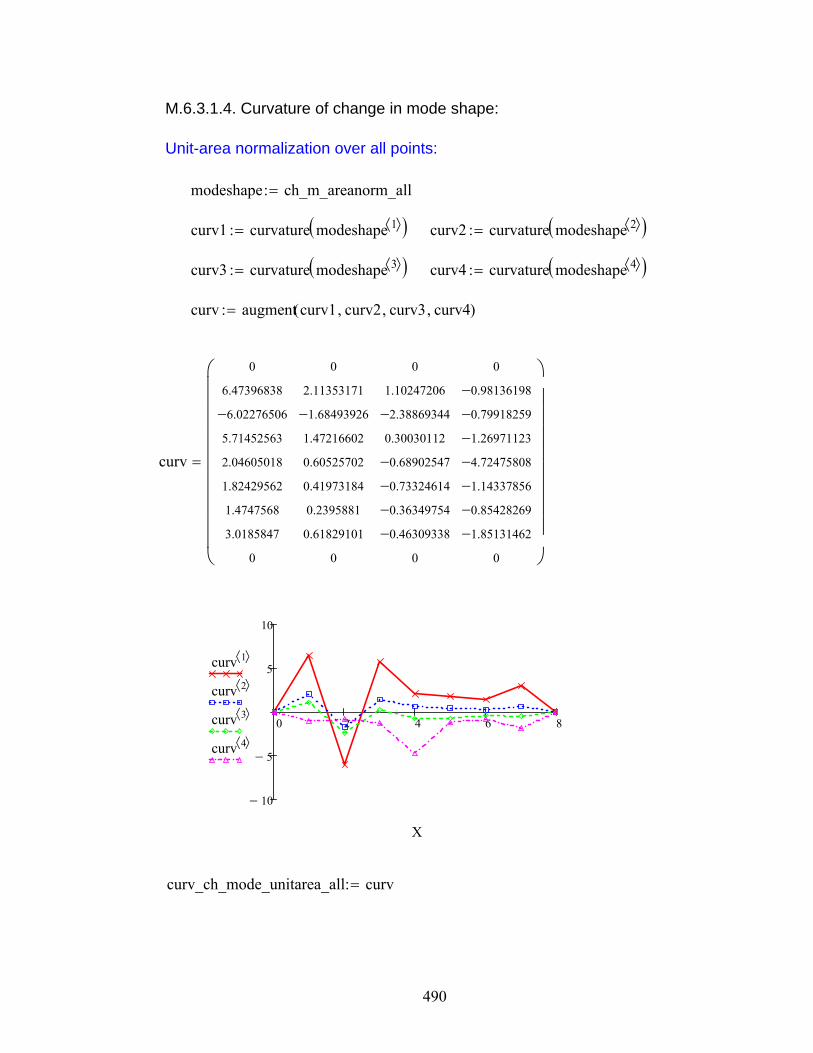
490
M.6.3.1.4. Curvature of change in mode shape:
Unit-area normalization over all points:
modeshape ch_m_areanorm_all
curv1 curvature modeshape 1 curv2 curvature modeshape 2
curv3 curvature modeshape 3 curv4 curvature modeshape 4
curv augment curv1 curv2 curv3 curv4( )
curv
0
6.47396838
6.022765065.71452563
2.04605018
1.82429562
1.4747568
3.0185847
0
0
2.11353171
1.684939261.47216602
0.60525702
0.41973184
0.2395881
0.61829101
0
0
1.10247206
2.388693440.30030112
0.689025470.733246140.363497540.46309338
0
0
0.981361980.799182591.269711234.724758081.143378560.854282691.85131462
0
0 2 4 6 8
10
5
5
10
curv 1
curv 2
curv 3
curv 4
X
curv_ch_mode_unitarea_all curv

491
Unit-area normalization along individual girder lines:
modeshape ch_m_areanorm_xgrid
curv1 curvature modeshape 1 curv2 curvature modeshape 2
curv3 curvature modeshape 3 curv4 curvature modeshape 4
curv augment curv1 curv2 curv3 curv4( )
curv
0
3.44873907
6.447749893.34684691
0.12241453
0.04603558
0.09789171
0.113535040
0
1.28062234
1.817191040.87170432
0.09826131
0.039316610.11003712
0.01491213
0
0
1.80224698
1.870378750.8344679
0.091591680.17860141
0.05019014
0.12200058
0
0
1.39986989
0.50173843
0.6779488
2.578429440.62163251
0.43629402
0.10081043
0
0 2 4 6 8
8
6
4
2
2
4
curv 1
curv 2
curv 3
curv 4
X
curv_ch_mode_unitarea_xgrid curv
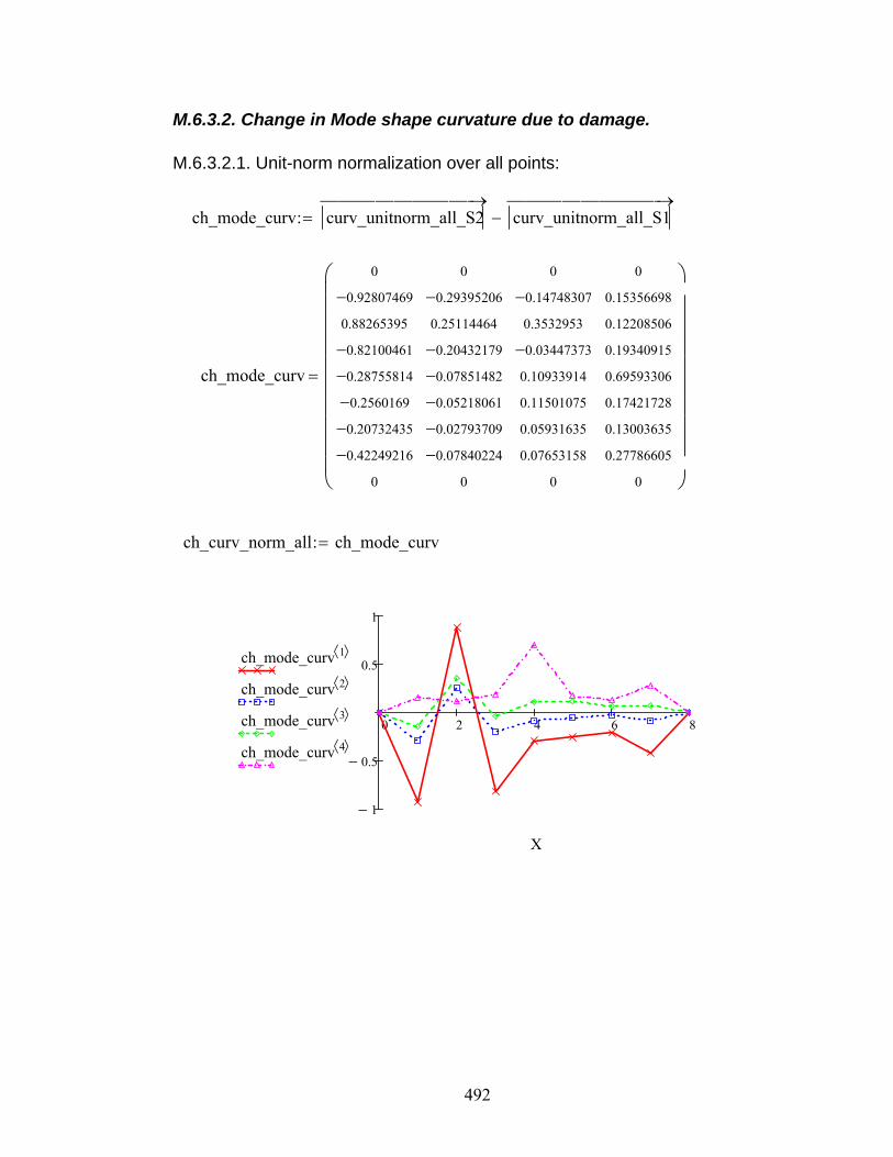
492
M.6.3.2. Change in Mode shape curvature due to damage.
M.6.3.2.1. Unit-norm normalization over all points:
ch_mode_curv curv_unitnorm_all_S2
curv_unitnorm_all_S1
ch_mode_curv
0
0.928074690.88265395
0.821004610.287558140.25601690.207324350.42249216
0
0
0.293952060.25114464
0.204321790.078514820.052180610.027937090.07840224
0
0
0.147483070.3532953
0.034473730.10933914
0.11501075
0.05931635
0.07653158
0
0
0.15356698
0.12208506
0.19340915
0.69593306
0.17421728
0.13003635
0.27786605
0
ch_curv_norm_all ch_mode_curv
0 2 4 6 8
1
0.5
0.5
1
ch_mode_curv 1
ch_mode_curv 2
ch_mode_curv 3
ch_mode_curv 4
X
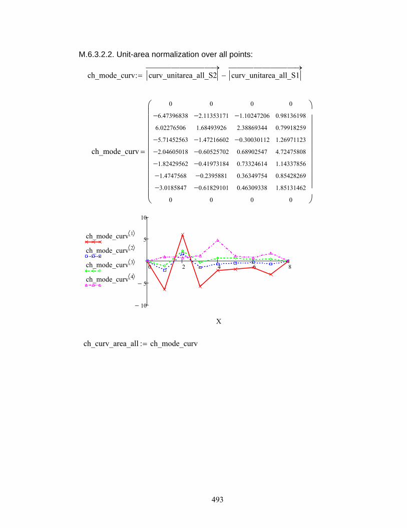
493
M.6.3.2.2. Unit-area normalization over all points:
ch_mode_curv curv_unitarea_all_S2
curv_unitarea_all_S1
ch_mode_curv
0
6.473968386.02276506
5.714525632.046050181.824295621.47475683.0185847
0
0
2.113531711.68493926
1.472166020.605257020.419731840.23958810.61829101
0
0
1.102472062.38869344
0.300301120.68902547
0.73324614
0.36349754
0.46309338
0
0
0.98136198
0.79918259
1.26971123
4.72475808
1.14337856
0.85428269
1.85131462
0
0 2 4 6 8
10
5
5
10
ch_mode_curv 1
ch_mode_curv 2
ch_mode_curv 3
ch_mode_curv 4
X
ch_curv_area_all ch_mode_curv

494
M.6.3.2.3. Unit-area normalization along individual girder lines:
ch_mode_curv curv_unitarea_xgrid_S2
curv_unitarea_xgrid_S1
ch_mode_curv
0
3.448739076.44774989
3.346846910.122414530.046035580.09789171
0.11353504
0
0
1.280622341.81719104
0.871704320.09826131
0.03931661
0.11003712
0.014912130
0
1.802246981.87037875
0.83446790.09159168
0.17860141
0.050190140.12200058
0
0
1.399869890.501738430.6779488
2.57842944
0.621632510.436294020.10081043
0
0 2 4 6 8
4
2
2
4
6
8
ch_mode_curv 1
ch_mode_curv 2
ch_mode_curv 3
ch_mode_curv 4
X
ch_curv_area_xgrid ch_mode_curv