Embed Size (px)
Citation preview

Vibration control by the use of apiezo actuator
V. van Geffen
DCT 2009.089
Traineeship report
Coach(es): ir. F. Huizinga
Supervisor: prof.dr.ir. M. Steinbuch
Technische Universiteit EindhovenDepartment Mechanical EngineeringDynamics and Control Technology Group
Eindhoven, September, 2009
Contents
1 Introduction 1
2 Modeling of a cantilever beam 3
2.1 Modeling . . . . . . . . . . . . . . . . . . . . . . . . . . . . . . . . . . . . . . . . 3
2.2 Model theory verification . . . . . . . . . . . . . . . . . . . . . . . . . . . . . . . 6
2.3 Model order reduction . . . . . . . . . . . . . . . . . . . . . . . . . . . . . . . . . 6
3 Simulation 9
3.1 Introduction . . . . . . . . . . . . . . . . . . . . . . . . . . . . . . . . . . . . . . 9
3.2 Normal modes . . . . . . . . . . . . . . . . . . . . . . . . . . . . . . . . . . . . . 9
3.3 Adding damping to the model . . . . . . . . . . . . . . . . . . . . . . . . . . . . . 10
4 Designing the study model 13
4.1 The basic parts . . . . . . . . . . . . . . . . . . . . . . . . . . . . . . . . . . . . . 13
4.1.1 The beam . . . . . . . . . . . . . . . . . . . . . . . . . . . . . . . . . . . . 13
4.1.2 The shaker . . . . . . . . . . . . . . . . . . . . . . . . . . . . . . . . . . . 14
4.1.3 The clamping structure . . . . . . . . . . . . . . . . . . . . . . . . . . . . 14
4.1.4 The sensor . . . . . . . . . . . . . . . . . . . . . . . . . . . . . . . . . . . 14
4.2 The actuator . . . . . . . . . . . . . . . . . . . . . . . . . . . . . . . . . . . . . . 15
4.2.1 Mounting the actuator . . . . . . . . . . . . . . . . . . . . . . . . . . . . . 15
4.3 Choosing the positions of the actuator, shaker and sensor . . . . . . . . . . . . . 16
i

ii CONTENTS
5 Test results 19
5.1 Linearity test . . . . . . . . . . . . . . . . . . . . . . . . . . . . . . . . . . . . . . 195.2 Frequency response measurements . . . . . . . . . . . . . . . . . . . . . . . . . . 20
Chapter 1
Introduction
The department CAE of the company PDE Automotive offers simulation and analysis services forautomobile parts. This work is mainly done to calculate the stiffness and strength of mechanicalparts. Modal analysis is applied as well to identify possible unwanted dynamics. Nowadays it iscommon to re-design parts when unwanted dynamics appear in simulations. A new area of inter-esse is to reduce or, when possible, totally remove this undesired behavior with vibration controltechnologies instead of re-designing. Possible benefits of this method are the savings of develop-ment and production costs, the interchangeability of car parts without an necessary pre-analysisand the possibility to cope with changing circumstances.To acquire the necessary acknowledge for vibration control a casestudy is performed. A beam isbeing clamped at one side and brought into vibration. An controller has to damp this vibrationwith the use of a piëzo-actuator. First this idea is simulated, later an demonstration model buildfor this study is used. Chapter 2 in this report treats the modeling of the beam. Since the com-pany works with finite elemental programs, it is logical to use these programs (with NASTRANspecifically in mind) for the production of the model. Since a great part of the experience andexpertise of the CAE lies within the use of these programs the importance to fully exploit thesefor further use is emphasized. A part of the study is used for investigating how this programexports the modeldata and how it has been manipulated. Chapter 3 reviews how this data canbe processed and used for simulations. Chapter 4 will show how the demonstration model isdesigned and how other decisions where made regarding the study model. And finally chapter 5will discuss the results.
1

2 CHAPTER 1. INTRODUCTION

Chapter 2
Modeling of a cantilever beam
2.1 Modeling
For modeling a beam that is clamped at one side and free at the other side (see figure 2.1) theEuler-Bernoulli beam theory is used. The Euler-Bernoulli beam model, for time-dependent load-ing, is governed by the partial differential equation
ρ∂2υ(x, t)
∂t2+
∂2
∂x2
(EI
∂2υ(x, t)∂x2
)= f(x, t) (2.1)
where υ(x, t) is the transverse displacement of the beam, ρ the mass density per volume, EI therigidity, f(x, t) the externally applied pressure loading and t and x indicate time and spatial axisalong the beam axis. The following assumptions are made
- There is an axis of the beam which undergoes no extension or contraction. The x-axis islocated along this neutral axis.
- Cross sections perpendicular to the neutral axis in the undeformed beam remain plane andremain perpendicular to the deformed neutral axis, that is, transverse shear deformation isneglected.
- The material is linearly elastic and the beam is homogeneous at any cross section.
- σy and σz are negligible compared to σx.
- The xy-plane is a principal plane.
The beam is divided into an infinite amount of smaller beam-elements. One short beam-element is being taken for further consideration (see figure 2.2). This element contains 2 nodes,each able to translate in the y-direction (υi) and rotate around the z-axis (ϕi). For continuity eachelement should have the same deflection and slope comparing to the neighboring elements.The Euler-Bernoulli beam equation is based on the assumption that the plane normal to theneutral axis before deformation remains normal to the neutral axis after deformation. This as-sumption yields ϕ = dυ/dx. The method of weighted residual, Galerkin’s method, is being
3
4 CHAPTER 2. MODELING OF A CANTILEVER BEAM
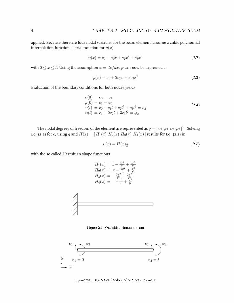
applied. Because there are four nodal variables for the beam element, assume a cubic polynomialinterpolation function as trial function for υ(x)
υ(x) = c0 + c1x + c2x2 + c3x
3 (2.2)
with 0 ≤ x ≤ l. Using the assumption ϕ = dυ/dx, ϕ can now be expressed as
ϕ(x) = c1 + 2c2x + 3c3x2 (2.3)
Evaluation of the boundary conditions for both nodes yields
υ(0) = c0 = υ1
ϕ(0) = c1 = ϕ1
υ(l) = c0 + c1l + c2l2 + c3l
3 = υ2
ϕ(l) = c1 + 2c2l + 3c3l2 = ϕ2
(2.4)
The nodal degrees of freedom of the element are represented as q = [ υ1 ϕ1 υ2 ϕ2 ]T . SolvingEq. (2.2) for ci using q and H(x) = [ H1(x) H2(x) H3(x) H4(x) ] results for Eq. (2.2) in
υ(x) = H(x)q (2.5)
with the so called Hermitian shape functions
H1(x) = 1− 3x2
l2+ 2x3
l3
H2(x) = x− 2x2
l + x3
l2
H3(x) = 3x2
l2− 2x3
l3
H4(x) = −x2
l + x3
l2
Figure 2.1: One-sided clamped beam
r r
6 6
υ1 ϕ1 υ2 ϕ2
-6 x
yx1 = 0 x2 = l
Figure 2.2: Degrees of freedom of one beam element

2.1. MODELING 5
Using this expression for υ and the Galerkin’s method (see [3] for further details) the second termof Eq. (2.1) results in the stiffness matrix of the beam element as follows
Ke =∫ l
0BT EIBdx (2.6)
whereB = H ′′ = [ H ′′
1 H ′′2 H ′′
3 H ′′4 ] (2.7)
Assuming a homogeneous beam, the element stiffness matrix becomes
Ke =2EI
l3
6 3l −6 3l3l 2l2 −3l l2
−6 −3l 6 −3l3l l2 −3l 2l2
(2.8)
Comparable with this last solution the first term of Eq. (2.1) results in the element mass matrixas follows
M e =∫ l
0ρAHT Hdx (2.9)
M e =ρlA
420
156 22l 54 −13l22l 4l2 13l −3l2
54 13l 156 −22l2
−13l −3l2 −22l2 4l2
(2.10)
known as the consistent mass matrix. Now damping can be added accordingly to the Rayleighdamping for example like
C = αM + βK (2.11)with the parameters α and β left to be determined. The element-forces acting on the nodalfreedoms can be expressed as ue(t) = [ Y1 M1 Y2 M2 ]T (see figure 2.3).
r r
6 6
Y1 M1 Y2 M2
-6 x
yx1 = 0 x2 = l
Figure 2.3: Forces acting on the element nodes
Instead of dividing the beam into an infinite amount of elements, it is customary to assumethat the displacements can be represented with good fidelity by an finite amount of elements. Thejustification for this assumption is that the bandwidths of actuators and sensors cannot sufficethe highest frequency modes. By choosing the amount of elements sufficiently large, the flexiblesystem is described adequately for the frequencies of interest. Adding the element matrixestogether, the beam dynamics can now be expressed as
Mq(t) + Cq(t) + Kq(t) = Fu(t) (2.12)with the force u(t) applied to the dof pointed out by the vector F.
6 CHAPTER 2. MODELING OF A CANTILEVER BEAM
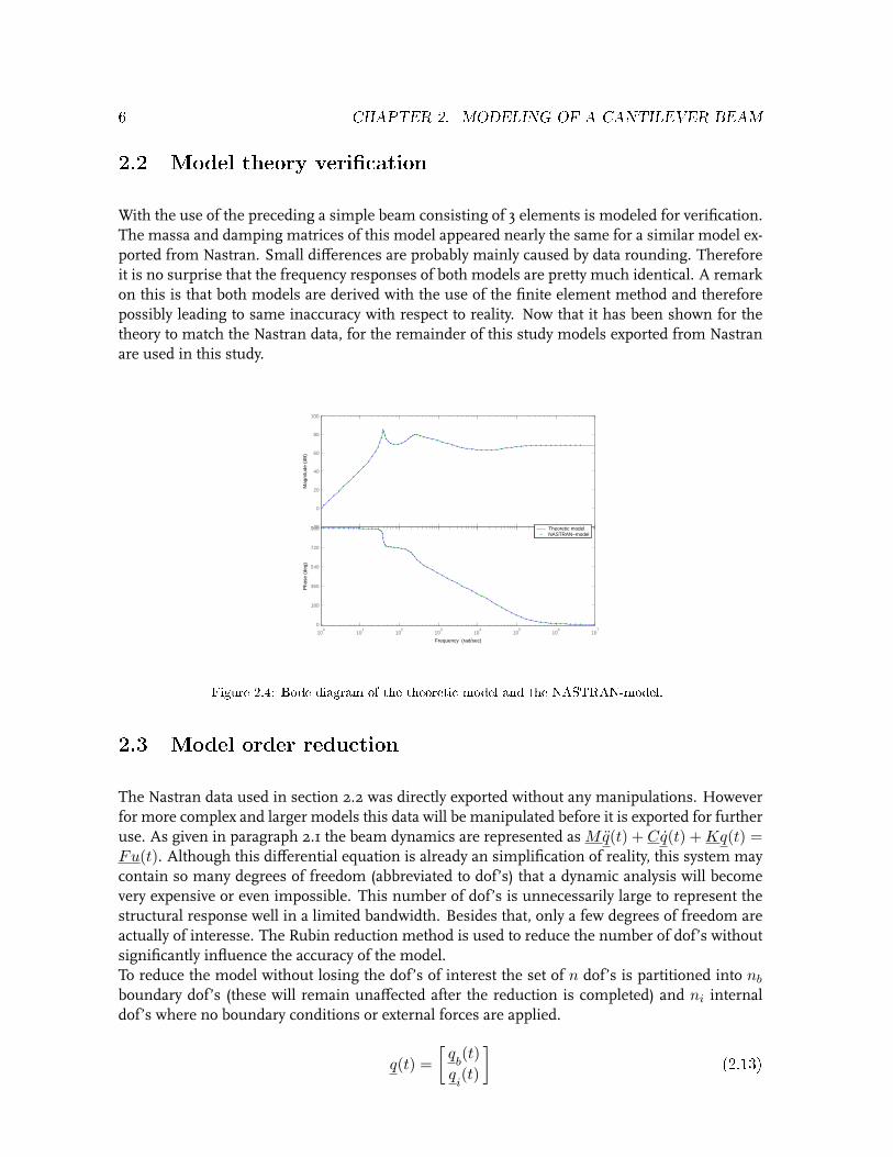
2.2 Model theory verication
With the use of the preceding a simple beam consisting of 3 elements is modeled for verification.The massa and damping matrices of this model appeared nearly the same for a similar model ex-ported from Nastran. Small differences are probably mainly caused by data rounding. Thereforeit is no surprise that the frequency responses of both models are pretty much identical. A remarkon this is that both models are derived with the use of the finite element method and thereforepossibly leading to same inaccuracy with respect to reality. Now that it has been shown for thetheory to match the Nastran data, for the remainder of this study models exported from Nastranare used in this study.
−20
0
20
40
60
80
100
Mag
nitu
de (
dB)
100
101
102
103
104
105
106
107
0
180
360
540
720
900
Pha
se (
deg)
Theoretic modelNASTRAN−model
Frequency (rad/sec)
Figure 2.4: Bode diagram of the theoretic model and the NASTRAN-model.
2.3 Model order reduction
The Nastran data used in section 2.2 was directly exported without any manipulations. Howeverfor more complex and larger models this data will be manipulated before it is exported for furtheruse. As given in paragraph 2.1 the beam dynamics are represented as Mq(t) + Cq(t) + Kq(t) =Fu(t). Although this differential equation is already an simplification of reality, this system maycontain so many degrees of freedom (abbreviated to dof’s) that a dynamic analysis will becomevery expensive or even impossible. This number of dof’s is unnecessarily large to represent thestructural response well in a limited bandwidth. Besides that, only a few degrees of freedom areactually of interesse. The Rubin reduction method is used to reduce the number of dof’s withoutsignificantly influence the accuracy of the model.To reduce the model without losing the dof’s of interest the set of n dof’s is partitioned into nb
boundary dof’s (these will remain unaffected after the reduction is completed) and ni internaldof’s where no boundary conditions or external forces are applied.
q(t) =[
qb(t)
qi(t)
](2.13)
2.3. MODEL ORDER REDUCTION 7
The system structure can be partitioned accordingly into[M bb M bi
M ib M ii
] [qb(t)
qi(t)
]+
[Kbb Kbi
Kib Kii
] [qb(t)
qi(t)
]=
[F b(t)Oi
](2.14)
Next an matrix B (which points out one boundary dof and the related data per column) is definedas
B =[
Ibb
Oib
](n∗nb)
(2.15)
Looking at the undamped system the following eigenvalue problem is associated
[K − λM ]u = 0 (2.16)
with n possible solutions for λ and u which are the eigenvalues and eigencolumns. Gatheringthe eigenvalues in the diagonal matrix Λ and the eigencolumns in the matrix U gives
Λ =
λ1
λ2
. . .λn
; U = [u1, u2, . . . , un] (2.17)
Assume that the eigenvalues are sorted as: λ1 ≤ λ2 ≤ . . . ≤ λn, so
MUΛ = KU ; UT MU = I; UT KU = Λ (2.18)
In case of a model with a large amount of dof’s, the frequencies corresponding to the highestmodes may exceed the frequency band of interest by far. For that reason the matrices Λ andU are partitioned as well into a part of kept-modes (indexed by k, k = 1, 2, . . . , nk) and a partof deleted-modes (indexed by d, d = nk + 1, nk + 2, . . . , n) which will be compensated. Thepartitioning leads to
Λ =[
Λkk Okd
Odk Λdd
]; U = [Uk, Ud] (2.19)
Assuming the model does not contain any rigid body mode, the residual flexibility modes can bestated as
Φ = UdΛ−1dd UT
d B = (K−1 − UkΛ−1kk UT
k )B = GresB (2.20)with Gres the residual flexibility matrix. Finally the transformation matrix R is
R = [Uk,Φ]n∗(nk+nb) (2.21)
so thatq(t) = Rp(t) (2.22)
Transformation reduces the model into
M redp(t) + Kredp(t) = F redu(t) (2.23)
whereM red = RT MR; Kred = RT KR; F red = RT F (t) (2.24)
8 CHAPTER 2. MODELING OF A CANTILEVER BEAM
The initial dof’s were the physical coordinates q(t) and are now changed to generalized dof’s p(t).For further use of the model the physical boundary dof’s are necessary and has to be recoveredwith an additional transformation (known as the coupling procedure of Martinez).[
qb(t)
qi(t)
]=
[U bb U bf
U ib U if
][p
b(t)
pf(t)
](2.25)
The partitioned column pf(t) contains the modal coordinates related to the free-interface modes.
The first subset of Eq. (2.25) is
qb(t) = U bbpb
(t) + U bfpf(t) (2.26)
which givesp
b(t) = U−1
bb qb(t)− U−1
bb U bfpf(t) (2.27)
This results in the following transformation
p(t) =
[p
b(t)
pf(t)
]=
[U−1
bb −U−1bb U bf
Ofb Iff
][qb(t)
pf(t)
]= Tp∗(t) (2.28)
which completes the reduction into
q(t) =[
qb(t)
qi(t)
]= RT
[qb(t)
pf(t)
]= Rtotp
∗(t) (2.29)
where qb(t) are the necessary physical dof’s and p
f(t) are the compensating residual dof’s.
Chapter 3
Simulation
3.1 Introduction
In the FEM program NASTRAN the beam is modeled and the system matrixes M , C and K areexported to MATLAB into equation
Mq(t) + Cq(t) + Kq(t) = Fu(t) (3.1)
For the simulation and further analysis of the beam dynamics, this equation has to be rewritteninto an first order state space formulation. The state vector is introduced as
x(t) =[
q(t)q(t)
](3.2)
Equation (3.1) can now be expressed like
x(t) =[
q(t)q(t)
]=
[0 I
−M−1K −M−1C
] [q(t)q(t)
]+
[0
M−1F
]u(t)
= Ax(t) + Bu(t)(3.3)
In this equation the inverse of M is taken. This calculation unfortunately lacks numerical accu-racy because of the ill-conditioned matrix M . This problem is solved using the normal modesdescribed next. The exported data from NASTRAN is reduced using the Rubin method describedbefore. The resulting added compensating residual dof’s are undamped which unfortunatelybrings another numerical problem with it. This will be discussed in section 3.3.
3.2 Normal modes
The Rubin reduction method, described in section 2.3, is similar for a part to the normal modes.Hereby the eigenvalue problem is addressed as well. A structure without rigid body modes isassumed without damping to begin with.
[K − λM ]u = 0 (3.4)
9

10 CHAPTER 3. SIMULATION
which lead to
Λ =
λ1
λ2
. . .λn
; U = [u1, u2, . . . , un] (3.5)
The normal mode matrix U can now be used as a coordinate transformation matrix as
q = Uη (3.6)
The normal mode vectors un are generalized orthogonal, which means that the mass, stiffnessand damping matrices can be diagonalized with an congruence transformation. A congruencetransformation is performed by pre-multiplying by the transpose of the coordinate transformationmatrix and then post-multiplying by same transformation matrix. This leads for the mass matrixto
UT MU =
. . .
dn
. . .
(3.7)
By orthonormalize the normal mode vectors un with respect to the mass, the corresponding dn
becomes equal to one. Pre-multiplying with UT and transformation of Eq. 3.1 now leads to thenew system equation
η(t) + Cnη(t) + Λη(t) = UT Fu(t) (3.8)with diagonal matrixes
UT MU = I; UT CU = Ω; UT KU = Λ (3.9)
whereΩ = diag(2ξnωn); Λ = diag(ω2
n) (3.10)ωn stands for the natural frequency of each mode, ξn for the viscous damping factor. The newsystem equations are completely uncoupled and the mass matrix is reduced to an identity matrixcontaining only ones so that a new first order state space can be formulated by
s(t) =[
η(t)η(t)
]=
[0 I−Λ −Ω
] [η(t)η(t)
]+
[0
UT F
]u(t)
= Ans(t) + Bnu(t)(3.11)
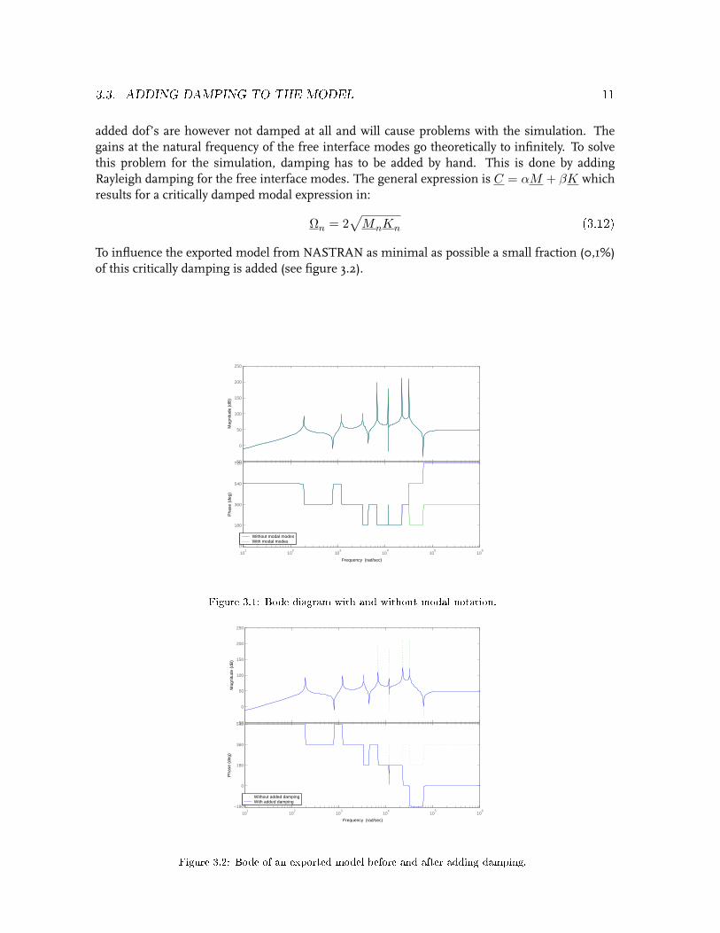
This formulation has the advantage that the inverse of M does not have to be calculated, makingthe result numerical more reliable. The resulting states of this equations are generalized. To re-sult in physical dof’s the generalized dof’s η(t) have to be transformed back into the original dof’sq(t). After this transformation the model represents the original model again without modifyingit, see figure 3.1.
3.3 Adding damping to the model
The system model exported from NASTRAN is reduced with the Rubin method to simplify thismodel without reducing the accuracy significantly. The exported model consist partially of phys-ical dof’s and for a part of compensating residual dof’s. The resonances that belong with these
3.3. ADDING DAMPING TO THE MODEL 11
added dof’s are however not damped at all and will cause problems with the simulation. Thegains at the natural frequency of the free interface modes go theoretically to infinitely. To solvethis problem for the simulation, damping has to be added by hand. This is done by addingRayleigh damping for the free interface modes. The general expression is C = αM + βK whichresults for a critically damped modal expression in:
Ωn = 2√
MnKn (3.12)
To influence the exported model from NASTRAN as minimal as possible a small fraction (0,1%)of this critically damping is added (see figure 3.2).
−50
0
50
100
150
200
250
Mag
nitu
de (
dB)
101
102
103
104
105
106
0
180
360
540
720
Pha
se (
deg)
Without modal modesWith modal modes
Frequency (rad/sec)
Figure 3.1: Bode diagram with and without modal notation.
−50
0
50
100
150
200
250
Mag
nitu
de (
dB)
101
102
103
104
105
106
−180
0
180
360
540
Pha
se (
deg)
Without added dampingWith added damping
Frequency (rad/sec)
Figure 3.2: Bode of an exported model before and after adding damping.

12 CHAPTER 3. SIMULATION
Chapter 4
Designing the study model
For the production of the study model a few parts had to be designed and produced, for examplethe beam and the structure that will hold the beam. Some other more standard parts could bepicked out of stock. The shaker, to bring the beam in vibration, and the sensor where alreadyavailable at PDE and could be used well for this research. The piezo actuator had been deliveredby a third party. In this chapter more details from these parts are being explained.
4.1 The basic parts
4.1.1 The beam
For designing the demonstration model, the cantilever beam, it’s obvious desired that the effectis taking place in a range of frequencies visible for the human eye. Therefore it has been chosenfor the beam to have its first resonance at around 30 Hz. Working with standard metal beamsavailable out of stock at PDE some dimensions and parameters are already determined with thelength of the beam still unknown.
E = Young’s modulusI = Area moment of inertia of beam cross sectionl = Length of beamρ = Mass density of beam materialA = Area of cross-section
fn =K
2π
√EI
ρAl4(4.1)
With K an coefficient, which is K = 3, 52 for a cantilever in its first eigenfrequency. Now itcan be calculated that the beam should have a length of 0,237 m in order to fulfill the desireddynamical behavior.
13
14 CHAPTER 4. DESIGNING THE STUDY MODEL
4.1.2 The shaker
The beam will be vibrated simply be the use of an electro-mechanic shaker connected to thebeam. The shaker will be used to create unwanted vibrations in the beam. The idea is of courseis to compensate for these unwanted vibrations with an actuator. The major drawback of using ashaker is that it needs to be connected to the beam somehow. In this case it is connected togetherwith a thin bar. Obviously this is going to influence the dynamic behavior of the beam making itmore difficult to model. In the case that its omitted in the model it will make it more difficult tocompare results from the model with the study model. As long as the amplitude of the vibrationof the beam is not extremely large, the influence of the connecting bar is not too much of aconcern. The intention is to stick to the elastic deformation of the beam anyway to prevent anydamage and keeping the dynamical behavior predictable.
4.1.3 The clamping structure
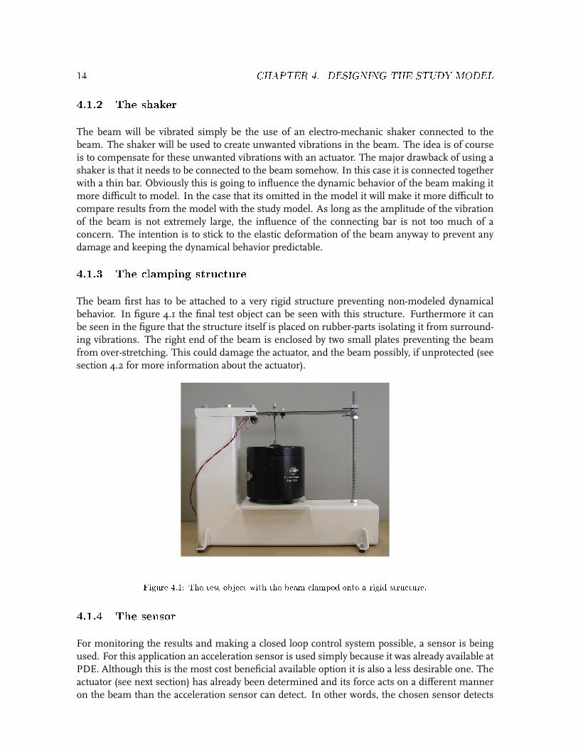
The beam first has to be attached to a very rigid structure preventing non-modeled dynamicalbehavior. In figure 4.1 the final test object can be seen with this structure. Furthermore it canbe seen in the figure that the structure itself is placed on rubber-parts isolating it from surround-ing vibrations. The right end of the beam is enclosed by two small plates preventing the beamfrom over-stretching. This could damage the actuator, and the beam possibly, if unprotected (seesection 4.2 for more information about the actuator).
Figure 4.1: The test object with the beam clamped onto a rigid structure.
4.1.4 The sensor
For monitoring the results and making a closed loop control system possible, a sensor is beingused. For this application an acceleration sensor is used simply because it was already available atPDE. Although this is the most cost beneficial available option it is also a less desirable one. Theactuator (see next section) has already been determined and its force acts on a different manneron the beam than the acceleration sensor can detect. In other words, the chosen sensor detects
4.2. THE ACTUATOR 15
the reaction of the actuator indirectly making this combination non-collocated. This will effectthe maximum possible bandwidth of the controlled system and its stability. A more favorableoption would be another piezo acting as a sensor. In that case the sensor could for example beplaced on the other side of the beam making it collocated.
4.2 The actuator
In this study a stacked ceramic multi-layer actuator (SCMA) is used for damping the beam. Theactuator has a cross section of 5 mm x 5 mm and a length of 8 mm. It has a maximum freedisplacement of 7 µm, an estimated blocking force of 1000 N and operates between 0 V and60 V . Mounting the actuator on the beam without any precaution would result in positive andnegative axial stress during the tests. But SCMA’s are sensitive to pulling forces so this has tobe prevented. Furthermore the displacement of the actuator would result in a force acting on thebeam in only one direction. A force acting in both direction is to be preferred for the best controleffectiveness and results. Therefore the actuator is being mounted on the beam under a pre-load.The amount of pre-load is taken half the maximum force the actuator can deliver. By taking anoffset voltage on the actuator the pre-load can be compensated for and the actuator is now ableto deliver a force on the beam in two directions. The static performances are influenced by theavailable stroke that is still left due to the offset, hysteresis, creep, stiffness and load capability.The maximum dynamic operating conditions are limited by the heating of the actuator causedby dielectric losses. Since the focus is mainly on the lower frequencies and by sticking to themaximum voltage, given by the manufacturer, this should not be of much influence.
4.2.1 Mounting the actuator
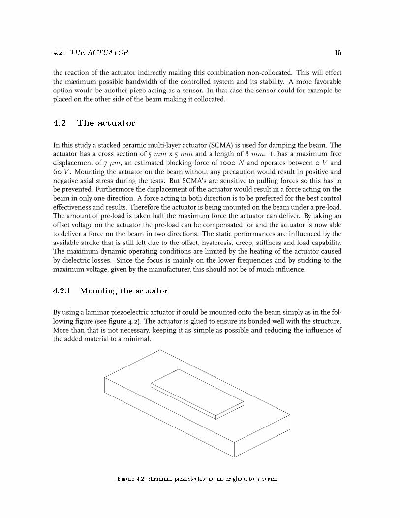
By using a laminar piezoelectric actuator it could be mounted onto the beam simply as in the fol-lowing figure (see figure 4.2). The actuator is glued to ensure its bonded well with the structure.More than that is not necessary, keeping it as simple as possible and reducing the influence ofthe added material to a minimal.
HHHHH
HHHHHH
HHHHHH
HHH
HHHHHH
HHHHHH
HHHHHH
HH
HHHH
HHHHHH
HHHHHH
HHHH
HHHH
HHHHHH
HHHHH
HHHHH
HHHH
HHHHHH
Figure 4.2: :Laminar piezoelectric actuator glued to a beam.
16 CHAPTER 4. DESIGNING THE STUDY MODEL
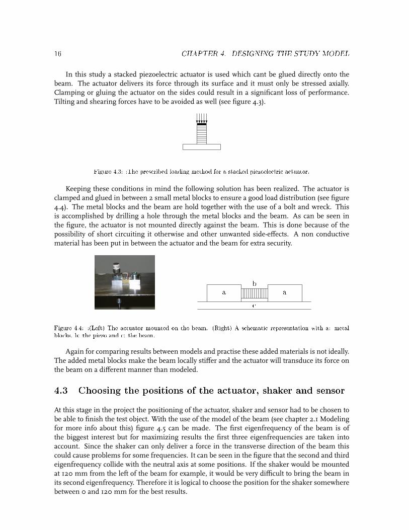
In this study a stacked piezoelectric actuator is used which cant be glued directly onto thebeam. The actuator delivers its force through its surface and it must only be stressed axially.Clamping or gluing the actuator on the sides could result in a significant loss of performance.Tilting and shearing forces have to be avoided as well (see figure 4.3).
?????
Figure 4.3: :The prescribed loading method for a stacked piezoelectric actuator.
Keeping these conditions in mind the following solution has been realized. The actuator isclamped and glued in between 2 small metal blocks to ensure a good load distribution (see figure4.4). The metal blocks and the beam are hold together with the use of a bolt and wreck. Thisis accomplished by drilling a hole through the metal blocks and the beam. As can be seen inthe figure, the actuator is not mounted directly against the beam. This is done because of thepossibility of short circuiting it otherwise and other unwanted side-effects. A non conductivematerial has been put in between the actuator and the beam for extra security.
a ab
c
Figure 4.4: :(Left) The actuator mounted on the beam. (Right) A schematic representation with a: metalblocks, b: the piezo and c: the beam.
Again for comparing results between models and practise these added materials is not ideally.The added metal blocks make the beam locally stiffer and the actuator will transduce its force onthe beam on a different manner than modeled.
4.3 Choosing the positions of the actuator, shaker and sensor
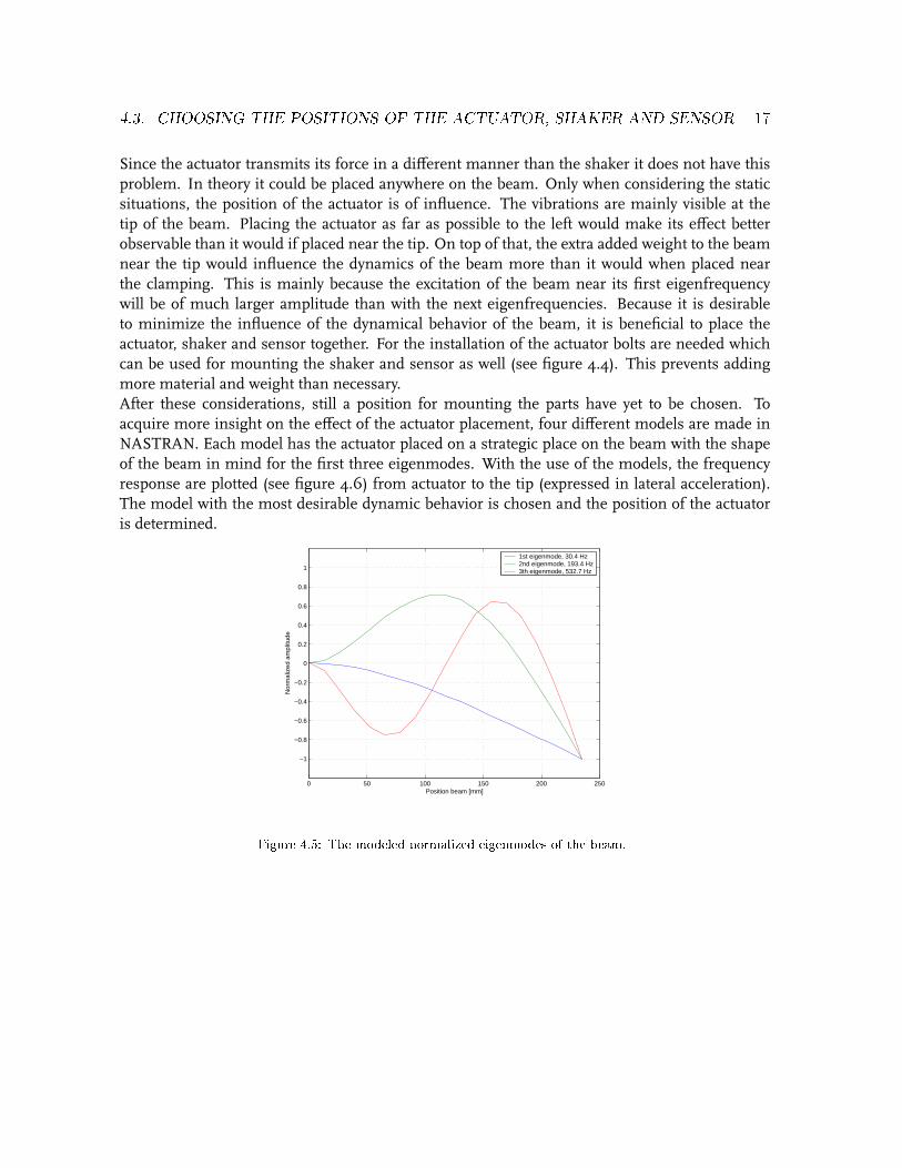
At this stage in the project the positioning of the actuator, shaker and sensor had to be chosen tobe able to finish the test object. With the use of the model of the beam (see chapter 2.1 Modelingfor more info about this) figure 4.5 can be made. The first eigenfrequency of the beam is ofthe biggest interest but for maximizing results the first three eigenfrequencies are taken intoaccount. Since the shaker can only deliver a force in the transverse direction of the beam thiscould cause problems for some frequencies. It can be seen in the figure that the second and thirdeigenfrequency collide with the neutral axis at some positions. If the shaker would be mountedat 120 mm from the left of the beam for example, it would be very difficult to bring the beam inits second eigenfrequency. Therefore it is logical to choose the position for the shaker somewherebetween 0 and 120 mm for the best results.
4.3. CHOOSING THE POSITIONS OF THE ACTUATOR, SHAKER AND SENSOR 17
Since the actuator transmits its force in a different manner than the shaker it does not have thisproblem. In theory it could be placed anywhere on the beam. Only when considering the staticsituations, the position of the actuator is of influence. The vibrations are mainly visible at thetip of the beam. Placing the actuator as far as possible to the left would make its effect betterobservable than it would if placed near the tip. On top of that, the extra added weight to the beamnear the tip would influence the dynamics of the beam more than it would when placed nearthe clamping. This is mainly because the excitation of the beam near its first eigenfrequencywill be of much larger amplitude than with the next eigenfrequencies. Because it is desirableto minimize the influence of the dynamical behavior of the beam, it is beneficial to place theactuator, shaker and sensor together. For the installation of the actuator bolts are needed whichcan be used for mounting the shaker and sensor as well (see figure 4.4). This prevents addingmore material and weight than necessary.After these considerations, still a position for mounting the parts have yet to be chosen. Toacquire more insight on the effect of the actuator placement, four different models are made inNASTRAN. Each model has the actuator placed on a strategic place on the beam with the shapeof the beam in mind for the first three eigenmodes. With the use of the models, the frequencyresponse are plotted (see figure 4.6) from actuator to the tip (expressed in lateral acceleration).The model with the most desirable dynamic behavior is chosen and the position of the actuatoris determined.
0 50 100 150 200 250
−1
−0.8
−0.6
−0.4
−0.2
0
0.2
0.4
0.6
0.8
1
Position beam [mm]
Nor
mal
ized
am
plitu
de
1st eigenmode, 30.4 Hz2nd eigenmode, 193.4 Hz3th eigenmode, 532.7 Hz
Figure 4.5: The modeled normalized eigenmodes of the beam.

18 CHAPTER 4. DESIGNING THE STUDY MODEL
102
103
104
0
20
40
60
80
100
120
Mag
nitu
de (
dB)
52.2 mm 65.3 mm104.4 mm117.5 mm
Frequency response from actuator to the tip (acceleration)
Frequency (rad/sec)
Figure 4.6: Frequency response from actuator to the tip-acceleration for dierent actuator placements.
Chapter 5
Test results
5.1 Linearity test
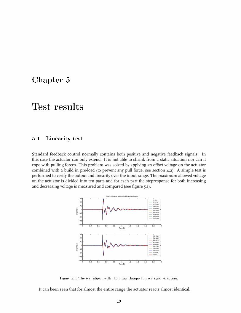
Standard feedback control normally contains both positive and negative feedback signals. Inthis case the actuator can only extend. It is not able to shrink from a static situation nor can itcope with pulling forces. This problem was solved by applying an offset voltage on the actuatorcombined with a build in pre-load (to prevent any pull force, see section 4.2). A simple test isperformed to verify the output and linearity over the input range. The maximum allowed voltageon the actuator is divided into ten parts and for each part the stepresponse for both increasingand decreasing voltage is measured and compared (see figure 5.1).
0 0.2 0.4 0.6 0.8 1 1.2 1.4 1.6 1.8 2−0.8
−0.6
−0.4
−0.2
0
0.2
0.4
0.6Stepresponse piezo at different voltages
Time [s]
Oup
ut [V
]
0−6 V6−12 V12−18 V18−24 V24−30 V30−36 V36−42 V42−48 V48−54 V54−60 V
0 0.2 0.4 0.6 0.8 1 1.2 1.4 1.6 1.8 2−0.8
−0.6
−0.4
−0.2
0
0.2
0.4
0.6
Time [s]
Oup
ut [V
]
60−54 V54−48 V48−42 V42−36 V36−30 V30−24 V24−18 V18−12 V12−6 V6−0 V
Figure 5.1: The test object with the beam clamped onto a rigid structure.
It can been seen that for almost the entire range the actuator reacts almost identical.
19

20 CHAPTER 5. TEST RESULTS
5.2 Frequency response measurements
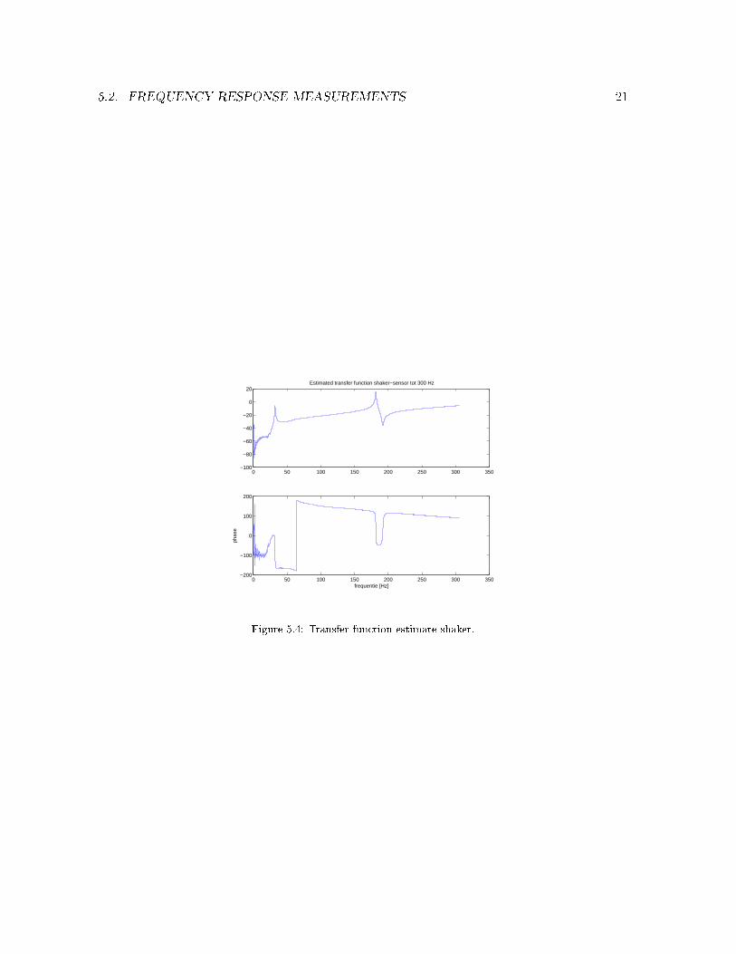
Frequency response measurements have been done for further analysis. As can be seen in thenext figures the coherence of the measurements from the shaker to the sensor are decent. Thecoherence from the piezo are not acceptable however. For further control applications and teststo be successful this has to be improved first.
0 50 100 150 200 2500.8
0.82
0.84
0.86
0.88
0.9
0.92
0.94
0.96
0.98
1coherence shaker
Frequency [Hz]
Figure 5.2: Coherence shaker.
0 10 20 30 40 50 60 70 80 90 1000
0.1
0.2
0.3
0.4
0.5
0.6
0.7
0.8
0.9
1Coherence piezo−sensor
Frequency [Hz]
Figure 5.3: Coherence piezo.
5.2. FREQUENCY RESPONSE MEASUREMENTS 21
0 50 100 150 200 250 300 350−100
−80
−60
−40
−20
0
20Estimated transfer function shaker−sensor tot 300 Hz
0 50 100 150 200 250 300 350−200
−100
0
100
200
frequentie [Hz]
phas
e
Figure 5.4: Transfer function estimate shaker.

22 CHAPTER 5. TEST RESULTS

Bibliography
[1] S. Hanagud, M.W. Obal and A.J. Calise, "Optimal vibration control by the use of piezoce-ramic sensors and actuators", Journal of Guidance, Control and Dynamics Volume 15, No. 5(1992)
[2] G.F. Franklin, J.D. Powell and A. Emami-Naeini, "Feedback control of dynamic systems"
[3] Y.W. Kwon and H. Bang, "The finite element method using MATLAB". Florida: CRC PressLLC, 1997.
[4] R.R. Craig, Jr., "Structural dynamics". Singapore: John Wiley & Sons, Inc., 1981.
[5] B. de Kraker, "A numerical experimental approach in structural dynamics". 2000.
[6] B. de Kraker and D.H. van Campen, "Mechanical vibrations". Maastricht: Shaker Publish-ing, 2001.
[7] A. Preumont, "Vibration control of active structures". Dordrecht: Kluwer Academic Pub-lishers, 2005.
23