Embed Size (px)
Citation preview
Shock and Vibration 10 (2003) 97–113 97IOS Press
Vibrational energy flow models of finiteorthotropic plates
Do-Hyun Parka, Suk-Yoon Honga,∗ and Hyun-Gwon KilbaDepartment of Naval Architecture and Ocean Engineering, Seoul National University, #56-1, Shinlim-dong,Kwanak-gu, Seoul 151-742, KoreabDepartment of Mechanical Engineering, The University of Suwon, Suwon 445-743, Korea
Abstract. In this paper energy flow models for the transverse vibration of finite orthotropic plates are developed. These modelsare expressed with time- and locally space-averaged far-field energy density, and show more general forms than the conventionalEFA models for isotropic plates. To verify the accuracy of the developed models, numerical analyses are performed for finiterectangular plates vibrating at a single frequency, and the calculated results expressed with the energy and intensity levels arecompared with those of classical models by changing the frequency and the damping.
1. Introduction
The Energy Flow Analysis (EFA) method has beendevelopedas a promising vibro-acousticprediction toolof medium-to-high frequency ranges. The EFA methodoffers an improved solution to the Statistical EnergyAnalysis (SEA) which does not give any informationon the energy variation in a subsystem and cannot con-sider the local power input and damping treatment. TheEFA model, analogous to the steady state heat flowmodel, was introduced by Belov et al. [13]. Nefskeand Sung [1] applied EFA to predict the flexural vi-bration of beams. Further studies for rods and beamswere performed by Wohlever and Bernhard [3,8,9].Bouthier and Bernhard [6–9] developed EFA modelsfor Kirchhoff-Love plates and membranes.
Many dynamic system structures such as ships andplanes include plate elements made of orthotropic ma-terials and stiffened or reinforced plates [5,10,11].These naturally and structurally orthotropic plates havedifferent bending stiffnesses in two perpendicular di-rections, on which the energy distribution and the pow-er transmission path depend greatly. Until now, thedevelopment of EFA models has been focused mainly
∗Corresponding author. Tel.: +82 2 880 8757; Fax: +82 2 8889298; E-mail: [email protected].
on isotropic structural elements, and more general en-ergy flow formulations are required to apply the EFAmethod properly to orthotropic structures.
The aim of this work is to develop approximate ener-gy flow models that predict the energy distribution andpower transmission path in a time- and locally space-averaged sense for the orthotropic plates vibrating inthe medium-to-high frequency ranges. Numerical anal-yses are performed for finite rectangular orthotropicplates which are simply supported along the edges andexcited by a transverse harmonic point force. The nu-merical results are compared between a classical modeland the derived EFA model for orthotropic plates, andthe effects of frequency and damping parameters areinvestigated.
2. Approximate energy flow models for thetransverse vibration of orthotropic plates
The equation of motion of thin orthotropic platesexcited by a harmonic point force located at (xo, yo) ofwhich the amplitude and the frequency areF andω,respectively, can be written as [5,11]:
Dxc∂4w
∂x4+ 2Hc
∂4w
∂x2∂y2
ISSN 1070-9622/03/$8.00 2003 – IOS Press. All rights reserved
98 D.-H. Park et al. / Vibrational energy flow models of finite orthotropic plates
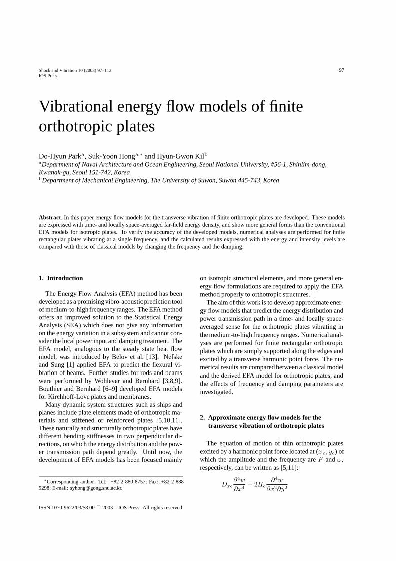
Fig. 1. The orthotropic plate response problem, displacement solution.
Fig. 2. The orthotropic plate response problem, energy solution.
+Dyc∂4w
∂y4+m
∂2w
∂t2(1)
= Fδ(x − xo)δ(y − yo)ejωt,
wherew is the transverse displacement andm is themass per unit area of the plate.Dxc andDyc are thecomplex bending stiffnesses in thex- andy-directions,respectively, and are written as
Dxc =Dx(1 + jη) and(2)
Dyc =Dy(1 + jη),
where η is the hysteretic damping loss factor.Hc
in Eq. (1) is the complex effective torsional stiffness.When the thickness of the plate is constant and its trans-verse displacement is relatively very small, its defor-mation being properly elastic, the effective torsionalstiffness,Hc, can be assumed to be the geometric meanof the bending stiffnessesDxc andDyc in the followingexpression [5]:
Hc =√DxcDyc. (3)
The effective torsional stiffness expressed by Eq. (3)makes it easy to mathematically handle the equation ofmotion given by Eq. (1). Despite of its preconditions,Cremer and Heckl [4] showed that Eq. (3) is a very goodapproximation for many practical orthotropic plates. Itcan be also seen in their work that the driving pointimpedance of an orthotropic plate is very nearly equal tothat of an homogeneous plate whose bending stiffness isequal to the geometric mean of the bending stiffnessesin the two coordinate direction. Substituting Eq. (3)into Eq. (1), the equation of motion is rewritten as
Dxc∂2w
∂x4+ 2√DxcDyc
∂4w
∂x2∂y2
+Dyc∂4w
∂y4+m
∂2w
∂t2(4)
= Fδ(x− xo)δ(y − yo)ejωt.
The authors of this paper investigate approximatepower flow models of the orthotropic plates withEq. (4).
D.-H. Park et al. / Vibrational energy flow models of finite orthotropic plates 99
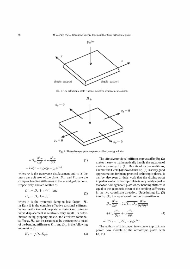
Fig. 3. The classical energy density distribution of the orthotropic plate whenf = 500 Hz andη = 0.02. The reference energy density is1 × 10−12 J/m2.
Fig. 4. The approximate energy density distribution of the orthotropic plate whenf = 500 Hz andη = 0.02. The reference energy density is1 × 10−12 J/m2.
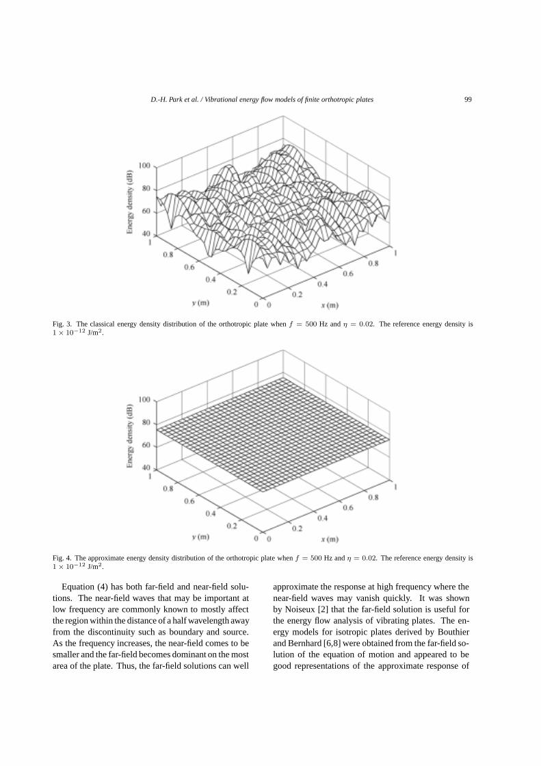
Equation (4) has both far-field and near-field solu-tions. The near-field waves that may be important atlow frequency are commonly known to mostly affectthe region within the distance of a half wavelength awayfrom the discontinuity such as boundary and source.As the frequency increases, the near-field comes to besmaller and the far-field becomes dominant on the mostarea of the plate. Thus, the far-field solutions can well
approximate the response at high frequency where thenear-field waves may vanish quickly. It was shownby Noiseux [2] that the far-field solution is useful forthe energy flow analysis of vibrating plates. The en-ergy models for isotropic plates derived by Bouthierand Bernhard [6,8] were obtained from the far-field so-lution of the equation of motion and appeared to begood representations of the approximate response of
100 D.-H. Park et al. / Vibrational energy flow models of finite orthotropic plates
Fig. 5. The classical intensity field in the orthotropic plate whenf = 500 Hz andη = 0.02.
the plates. Thus, in this work only the far-field solu-tions are utilized for relevant analyses. The generalfar-field solution can be expressed as the sum of theplane progressive wave components:
wff (x, y, t)
= (Ae−j(kxx+kyy) +Bej(kxx−kyy)
(5)+Ce−j(kxx−kyy) +Dej(kxx+kyy))ejωt,
wherekx andky are the complex wave numbers in thex- andy-directions, respectively.kxl andkyl are realparts ofkx andky, and then the dispersion relation isexpressed as(√
Dxk2xl +
√Dyk
2yl
)2
= ω2m. (6)
When the damping is small,kx andky are well ap-proximated by
kx = kxl
(1 − j η
4
)(7a)
and
ky = kyl
(1 − j η
4
). (7b)
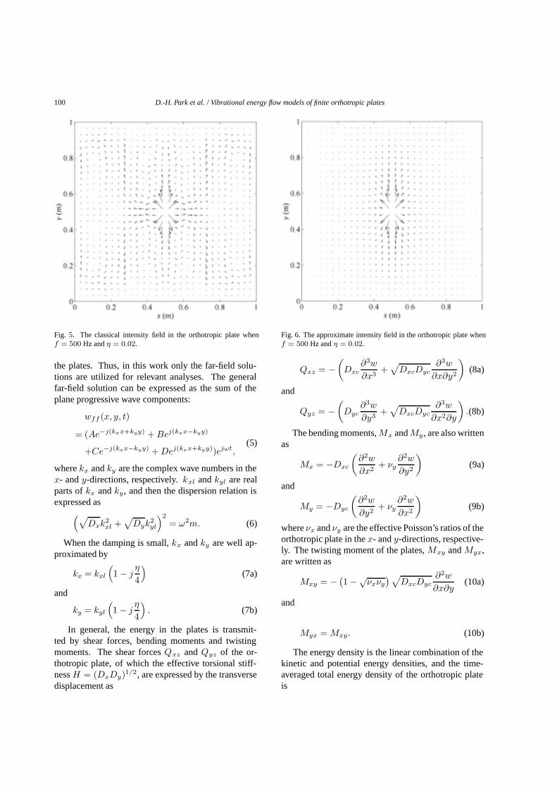
In general, the energy in the plates is transmit-ted by shear forces, bending moments and twistingmoments. The shear forcesQxz andQyz of the or-thotropic plate, of which the effective torsional stiff-nessH = (DxDy)1/2, are expressed by the transversedisplacement as
Fig. 6. The approximate intensity field in the orthotropic plate whenf = 500 Hz andη = 0.02.
Qxz = −(Dxc
∂3w
∂x3+√DxcDyc
∂3w
∂x∂y2
)(8a)
and
Qyz = −(Dyc
∂3w
∂y3+√DxcDyc
∂3w
∂x2∂y
).(8b)
The bending moments,Mx andMy, are also writtenas
Mx = −Dxc
(∂2w
∂x2+ νy
∂2w
∂y2
)(9a)
and
My = −Dyc
(∂2w
∂y2+ νy
∂2w
∂x2
)(9b)
whereνx andνy are the effective Poisson’s ratios of theorthotropic plate in thex- andy-directions, respective-ly. The twisting moment of the plates,Mxy andMyx,are written as
Mxy = − (1 −√νxνy
)√DxcDyc
∂2w
∂x∂y(10a)
and
Myx = Mxy. (10b)
The energy density is the linear combination of thekinetic and potential energy densities, and the time-averaged total energy density of the orthotropic plateis
D.-H. Park et al. / Vibrational energy flow models of finite orthotropic plates 101
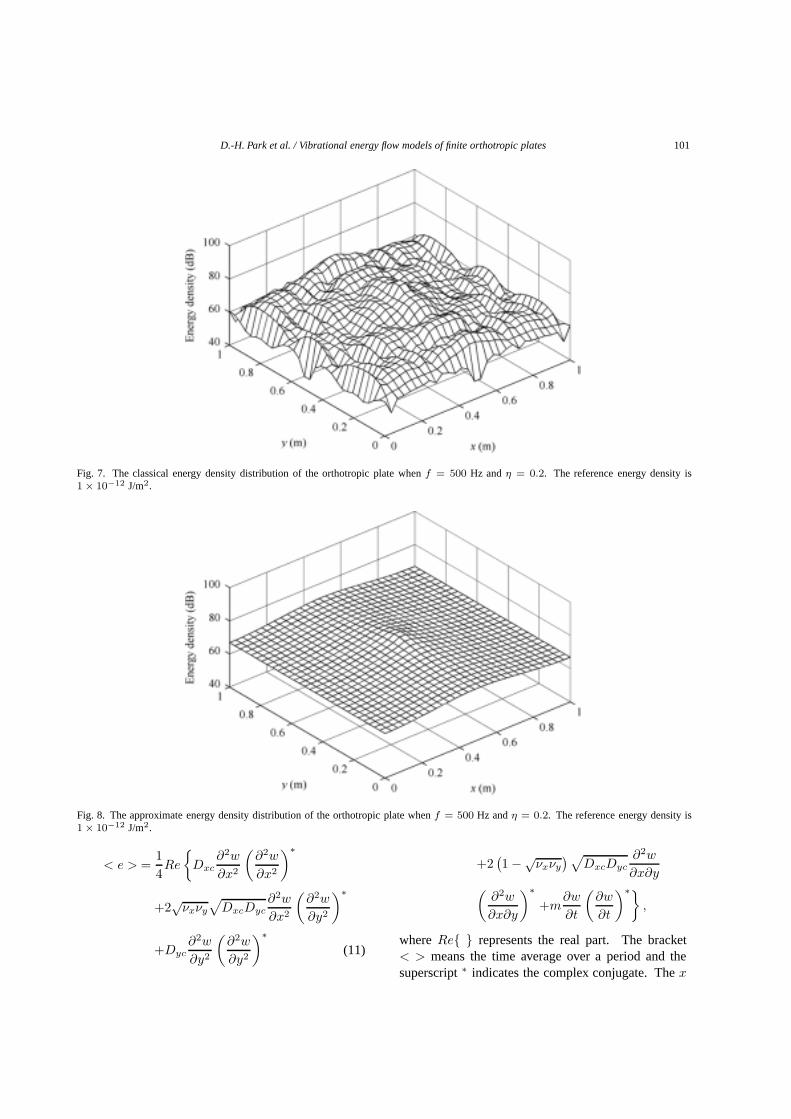
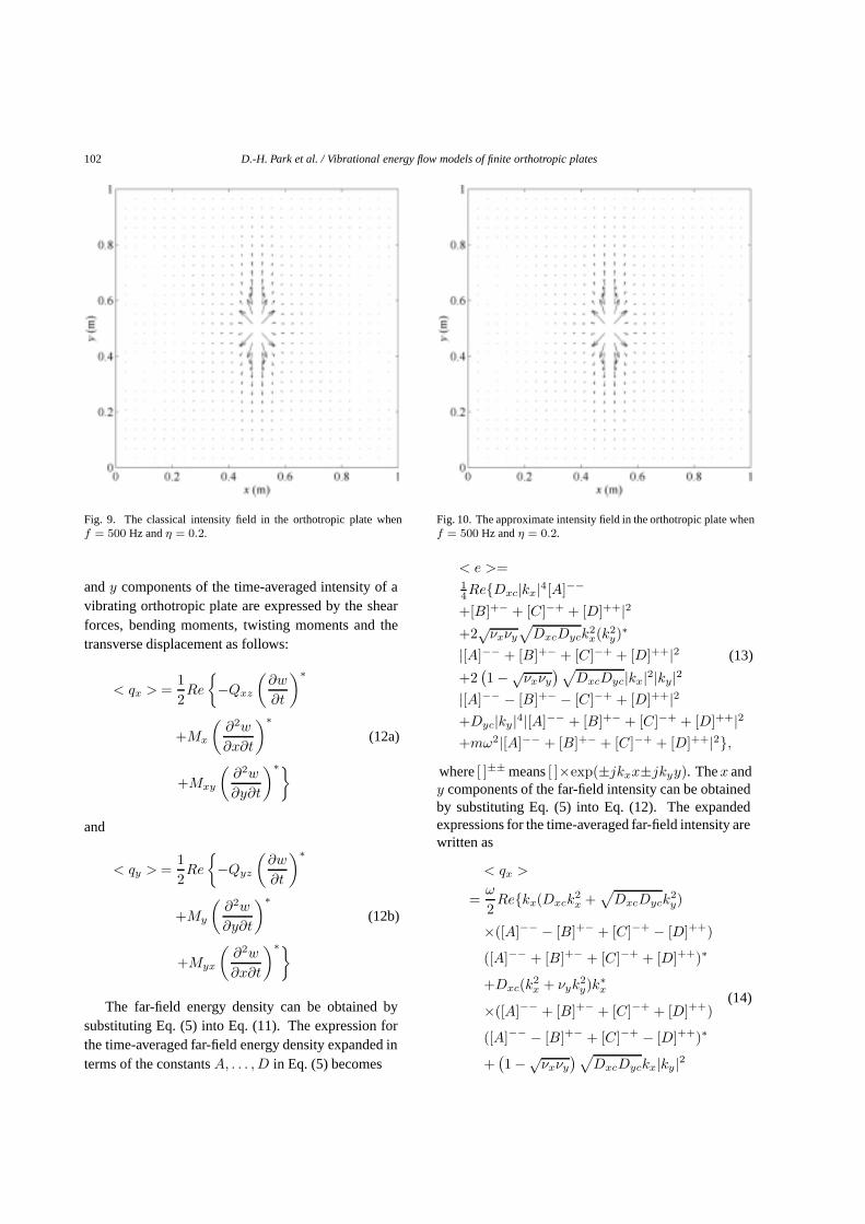
Fig. 7. The classical energy density distribution of the orthotropic plate whenf = 500 Hz andη = 0.2. The reference energy density is1 × 10−12 J/m2.
Fig. 8. The approximate energy density distribution of the orthotropic plate whenf = 500 Hz andη = 0.2. The reference energy density is1 × 10−12 J/m2.
< e > =14Re
{Dxc
∂2w
∂x2
(∂2w
∂x2
)∗
+2√νxνy
√DxcDyc
∂2w
∂x2
(∂2w
∂y2
)∗
+Dyc∂2w
∂y2
(∂2w
∂y2
)∗(11)
+2(1 −√
νxνy
)√DxcDyc
∂2w
∂x∂y(∂2w
∂x∂y
)∗+m
∂w
∂t
(∂w
∂t
)∗},
whereRe{ } represents the real part. The bracket< > means the time average over a period and thesuperscript∗ indicates the complex conjugate. Thex
102 D.-H. Park et al. / Vibrational energy flow models of finite orthotropic plates
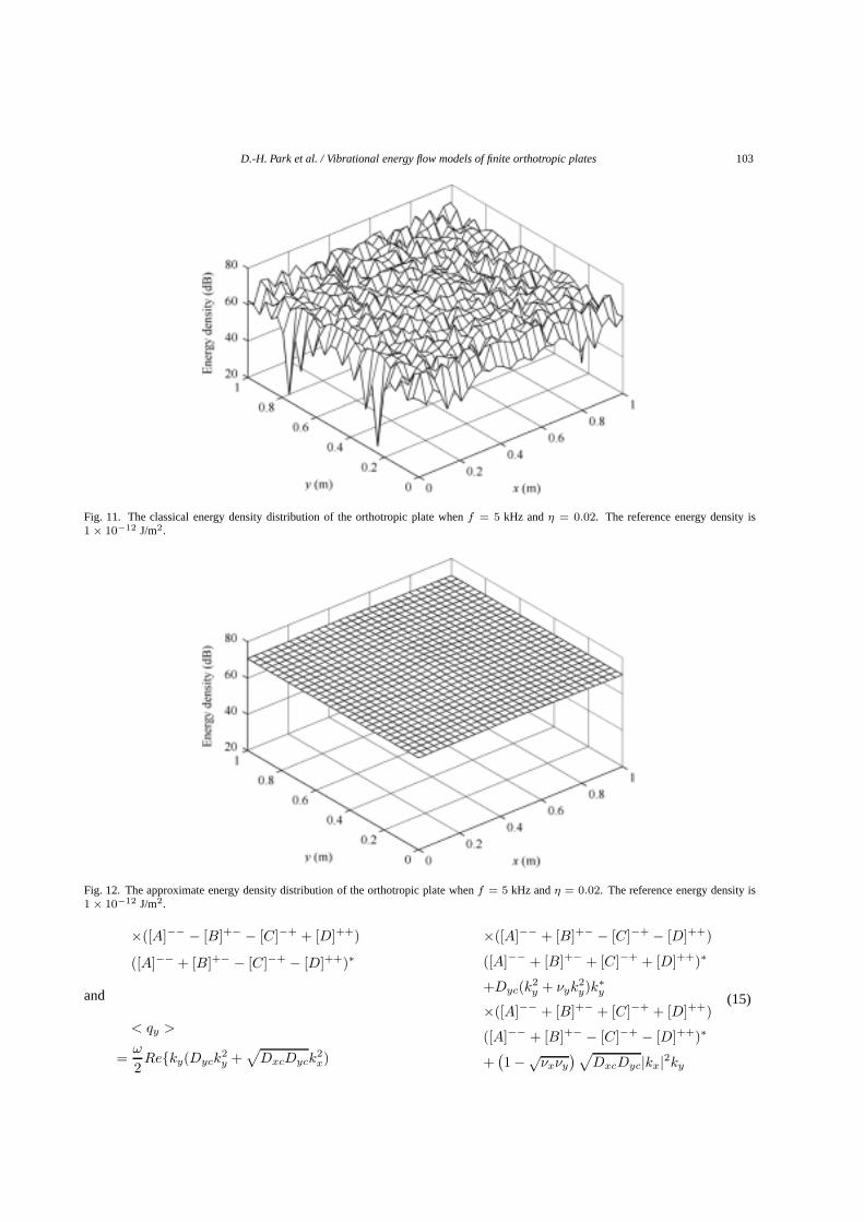
Fig. 9. The classical intensity field in the orthotropic plate whenf = 500 Hz andη = 0.2.
andy components of the time-averaged intensity of avibrating orthotropic plate are expressed by the shearforces, bending moments, twisting moments and thetransverse displacement as follows:
< qx > =12Re
{−Qxz
(∂w
∂t
)∗
+Mx
(∂2w
∂x∂t
)∗(12a)
+Mxy
(∂2w
∂y∂t
)∗}
and
< qy > =12Re
{−Qyz
(∂w
∂t
)∗
+My
(∂2w
∂y∂t
)∗(12b)
+Myx
(∂2w
∂x∂t
)∗}
The far-field energy density can be obtained bysubstituting Eq. (5) into Eq. (11). The expression forthe time-averaged far-field energy density expanded interms of the constantsA, . . . ,D in Eq. (5) becomes
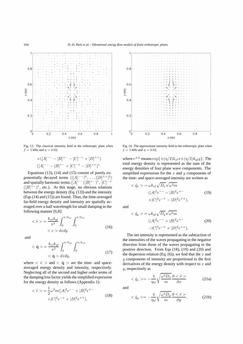
Fig. 10. The approximate intensity field in the orthotropic plate whenf = 500 Hz andη = 0.2.
< e >=14Re{Dxc|kx|4[A]−−
+[B]+− + [C]−+ + [D]++|2+2√νxνy
√DxcDyck
2x(k2
y)∗
|[A]−− + [B]+− + [C]−+ + [D]++|2+2(1 −√
νxνy
)√DxcDyc|kx|2|ky|2
|[A]−− − [B]+− − [C]−+ + [D]++|2+Dyc|ky|4|[A]−− + [B]+− + [C]−+ + [D]++|2+mω2|[A]−− + [B]+− + [C]−+ + [D]++|2},
(13)
where[ ]±± means[ ]×exp(±jkxx±jkyy). Thex andy components of the far-field intensity can be obtainedby substituting Eq. (5) into Eq. (12). The expandedexpressions for the time-averaged far-field intensity arewritten as
< qx >
=ω
2Re{kx(Dxck
2x +
√DxcDyck
2y)
×([A]−− − [B]+− + [C]−+ − [D]++)
([A]−− + [B]+− + [C]−+ + [D]++)∗
+Dxc(k2x + νyk
2y)k∗x
(14)×([A]−− + [B]+− + [C]−+ + [D]++)
([A]−− − [B]+− + [C]−+ − [D]++)∗
+(1 −√
νxνy
)√DxcDyckx|ky|2
D.-H. Park et al. / Vibrational energy flow models of finite orthotropic plates 103
Fig. 11. The classical energy density distribution of the orthotropic plate whenf = 5 kHz andη = 0.02. The reference energy density is1 × 10−12 J/m2.
Fig. 12. The approximate energy density distribution of the orthotropic plate whenf = 5 kHz andη = 0.02. The reference energy density is1 × 10−12 J/m2.
×([A]−− − [B]+− − [C]−+ + [D]++)
([A]−− + [B]+− − [C]−+ − [D]++)∗
and
< qy >
=ω
2Re{ky(Dyck
2y +
√DxcDyck
2x)
×([A]−− + [B]+− − [C]−+ − [D]++)
([A]−− + [B]+− + [C]−+ + [D]++)∗
+Dyc(k2y + νyk
2y)k∗y
(15)×([A]−− + [B]+− + [C]−+ + [D]++)
([A]−− + [B]+− − [C]−+ − [D]++)∗
+(1 −√
νxνy
)√DxcDyc|kx|2ky
104 D.-H. Park et al. / Vibrational energy flow models of finite orthotropic plates
Fig. 13. The classical intensity field in the orthotropic plate whenf = 5 kHz andη = 0.02.
×([A]−− − [B]+− − [C]−+ + [D]++)
([A]−− − [B]+− + [C]−+ − [D]++)∗
Equations (13), (14) and (15) consist of purely ex-ponentially decayed terms(|[A]−−|2, . . . , |[D]++|2)and spatially harmonic terms([A]−−([B]+−)∗, [C]−+
([B]+−)∗, etc.). At this stage, no obvious relationsbetween the energy density (Eq. (13)) and the intensity(Eqs (14) and (15)) are found. Thus, the time-averagedfar-field energy density and intensity are spatially av-eraged over a half wavelength for small damping in thefollowing manner [6,8]:
< e > =kxlkyl
π2
∫ π/kyl
0
∫ π/kxl
0 (16)< e > dxdy
and
< q > =kxlkyl
π2
∫ π/kyl
0
∫ π/kxl
0 (17)< q > dxdy,
where< e > and< q > are the time- and space-averaged energy density and intensity, respectively.Neglecting all of the second and higher order terms ofthe damping loss factor yields the simplified expressionfor the energy density as follows (Appendix 1):
< e > =12ω2m(|A|2e−− + |B|2e+−
(18)+|C|2e−+ + |D|2e++),
Fig. 14. The approximate intensity field in the orthotropic plate whenf = 5 kHz andη = 0.02.
wheree±± meansexp{±(η/2)kxlx±(η/2)kyly}. Thetotal energy density is represented as the sum of theenergy densities of four plane wave components. Thesimplified expressions for thex andy components ofthe time- and space-averaged intensity are written as
< qx > = ωkxl
√Dx
√ω2m
(|A|2e−− − |B|2e+− (19)
+|C|2e−+ − |D|2e++),
and
< qy > = ωkyl
√Dy
√ω2m
(|A|2e−− + |B|2e+− (20)
−|C|2e−+ + |D|2e++),
The net intensity is represented as the subtraction ofthe intensities of the waves propagating in the negativedirection from those of the waves propagating in thepositive direction. From Eqs (18), (19) and (20) andthe dispersion relation (Eq. (6)), we find that thex andy components of intensity are proportional to the firstderivatives of the energy density with respect tox andy, respectively as
< qx >= − 4ηω
√ω2Dx
m
∂ < e >
∂x(21a)
and
< qy >= − 4ηω
√ω2Dy
m
∂ < e >
∂y. (21b)
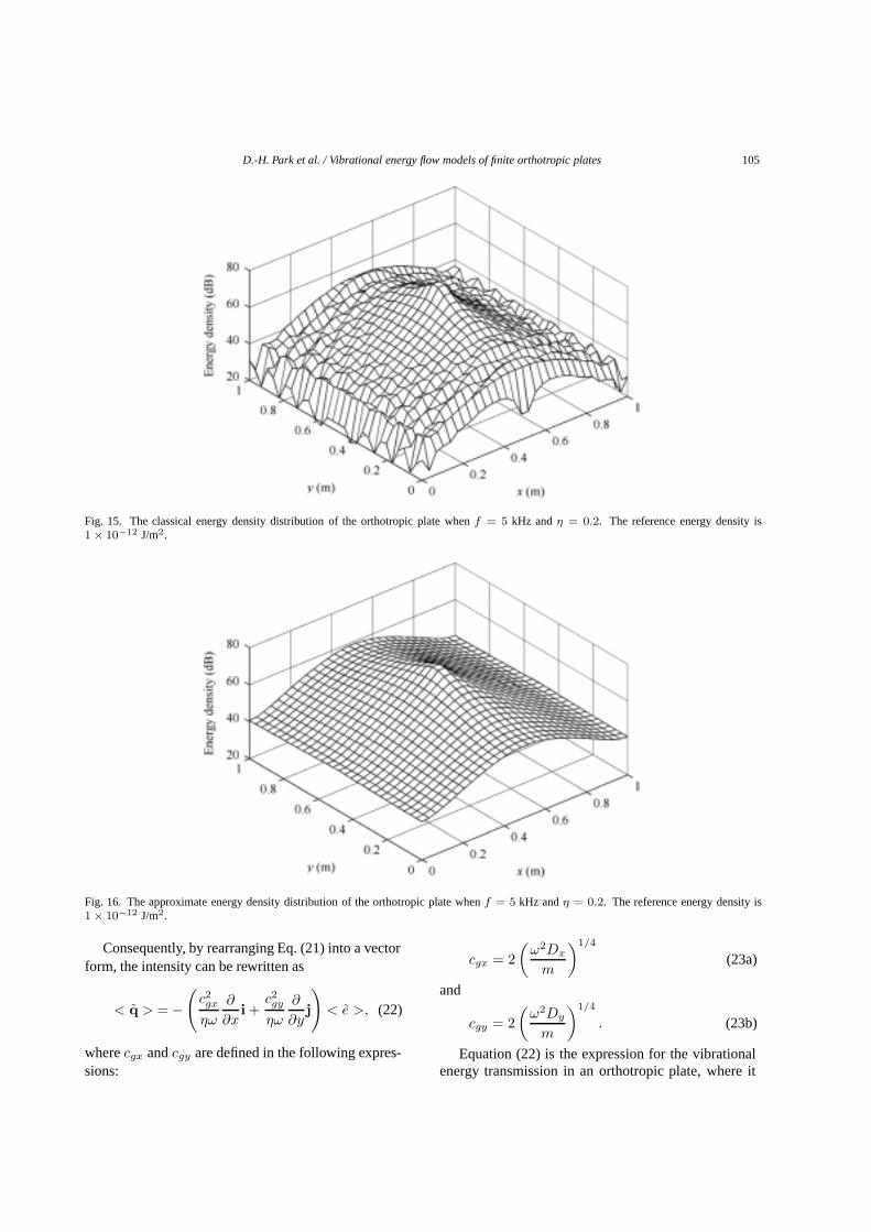
D.-H. Park et al. / Vibrational energy flow models of finite orthotropic plates 105
Fig. 15. The classical energy density distribution of the orthotropic plate whenf = 5 kHz andη = 0.2. The reference energy density is1 × 10−12 J/m2.
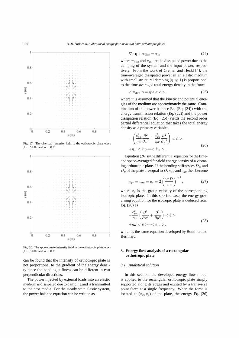
Fig. 16. The approximate energy density distribution of the orthotropic plate whenf = 5 kHz andη = 0.2. The reference energy density is1 × 10−12 J/m2.
Consequently, by rearranging Eq. (21) into a vectorform, the intensity can be rewritten as
< q > = −(c2gx
ηω
∂
∂xi +
c2gy
ηω
∂
∂yj
)< e >, (22)
wherecgx andcgy are defined in the following expres-sions:
cgx = 2(ω2Dx
m
)1/4
(23a)
and
cgy = 2(ω2Dy
m
)1/4
. (23b)
Equation (22) is the expression for the vibrationalenergy transmission in an orthotropic plate, where it
106 D.-H. Park et al. / Vibrational energy flow models of finite orthotropic plates
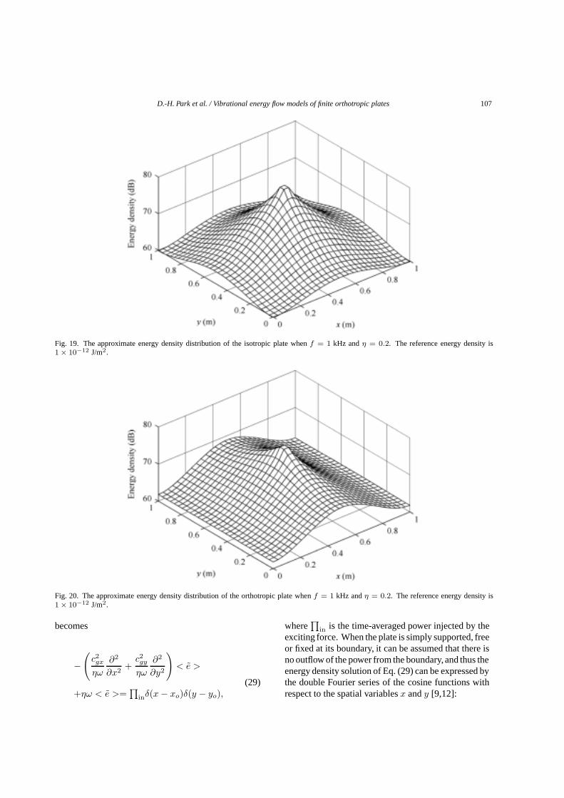
Fig. 17. The classical intensity field in the orthotropic plate whenf = 5 kHz andη = 0.2.
Fig. 18. The approximate intensity field in the orthotropic plate whenf = 5 kHz andη = 0.2.
can be found that the intensity of orthotropic plate isnot proportional to the gradient of the energy densi-ty since the bending stiffness can be different in twoperpendicular directions.
The power injected by external loads into an elasticmedium is dissipated due to damping and is transmittedto the next media. For the steady state elastic system,the power balance equation can be written as
∇ · q + πdiss = πin, (24)
whereπdiss andπin are the dissipated power due to thedamping of the system and the input power, respec-tively. From the work of Cremer and Heckl [4], thetime-averaged dissipated power in an elastic mediumwith small structural damping (η 1) is proportionalto the time-averaged total energy density in the form:
< πdiss >= ηω < e >, (25)
where it is assumed that the kinetic and potential ener-gies of the medium are approximately the same. Com-bination of the power balance Eq. (Eq. (24)) with theenergy transmission relation (Eq. (22)) and the powerdissipation relation (Eq. (25)) yields the second orderpartial differential equation that takes the total energydensity as a primary variable:
−(c2gx
ηω
∂2
∂x2+c2gy
ηω
∂2
∂y2
)< e >
(26)+ηω < e >=< πin > .
Equation (26) is the differential equation for the time-and space-averaged far-field energy density of a vibrat-ing orthotropic plate. If the bending stiffnessesDx andDy of the plate are equal toD, cgx andcgy then become
cgx = cgy = cg = 2(ω2D
m
)1/4
, (27)
wherecg is the group velocity of the correspondingisotropic plate. In this specific case, the energy gov-erning equation for the isotropic plate is deduced fromEq. (26) as
−c2gx
ηω
(∂2
∂x2+∂2
∂y2
)< e >
(28)+ηω < e >=< πin >,
which is the same equation developed by Bouthier andBernhard.
3. Energy flow analysis of a rectangularorthotropic plate
3.1. Analytical solution
In this section, the developed energy flow modelis applied to the rectangular orthotropic plate simplysupported along its edges and excited by a transversepoint force at a single frequency. When the force islocated at (xo, yo) of the plate, the energy Eq. (26)
D.-H. Park et al. / Vibrational energy flow models of finite orthotropic plates 107
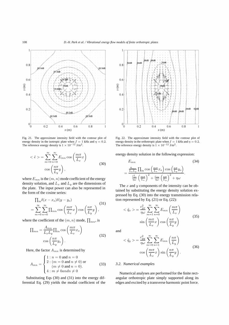
Fig. 19. The approximate energy density distribution of the isotropic plate whenf = 1 kHz andη = 0.2. The reference energy density is1 × 10−12 J/m2.
Fig. 20. The approximate energy density distribution of the orthotropic plate whenf = 1 kHz andη = 0.2. The reference energy density is1 × 10−12 J/m2.
becomes
−(c2gx
ηω
∂2
∂x2+c2gy
ηω
∂2
∂y2
)< e >
(29)+ηω < e >=
∏inδ(x− xo)δ(y − yo),
where∏
in is the time-averaged power injected by theexciting force. When the plate is simply supported, freeor fixed at its boundary, it can be assumed that there isno outflow of the power from the boundary,and thus theenergy density solution of Eq. (29) can be expressed bythe double Fourier series of the cosine functions withrespect to the spatial variablesx andy [9,12]:
108 D.-H. Park et al. / Vibrational energy flow models of finite orthotropic plates
Fig. 21. The approximate intensity field with the contour plot ofenergy density in the isotropic plate whenf = 1 kHz andη = 0.2.The reference energy density is1 × 10−12 J/m2.
< e > =∞∑
m=0
∞∑n=0
Emn cos(mπ
Lxx
)(30)
cos(nπ
Lyy
),
whereEmn is the(m,n) mode coefficient of the energydensity solution, andLx andLy are the dimensions ofthe plate. The input power can also be represented inthe form of the cosine series:∏
inδ(x − xo)δ(y − yo)(31)
=∞∑
m=0
∞∑n=0
∏mn cos
(mπ
Lxx
)cos(nπ
Lyy
),
where the coefficient of the(m,n) mode,∏
mn, is
∏mn =
Amn
LxLy
∏in cos
(mπ
Lxxo
)(32)
cos(nπ
Lyyo
).
Here, the factorAmn is determined by
Amn =
1 : n = 0 andn = 02 : (m = 0 andn �= 0) or
(m �= 0 andn = 0).4 : m �= 0andn �= 0
(33)
Substituting Eqs (30) and (31) into the energy dif-ferential Eq. (29) yields the modal coefficient of the
Fig. 22. The approximate intensity field with the contour plot ofenergy density in the orthotropic plate whenf = 1 kHz andη = 0.2.The reference energy density is1 × 10−12 J/m2.
energy density solution in the following expression:
Emn (34)
=Amn
LxLy
∏in cos
(mπLxxo
)cos(
nπLyyo
)c2
gx
ηω
(mπLx
)2
+ cgy
ηω
(nπLy
)2
+ ηω.
Thex andy components of the intensity can be ob-tained by substituting the energy density solution ex-pressed by Eq. (30) into the energy transmission rela-tion represented by Eq. (21) or Eq. (22):
< qx > =c2gx
ηω
∞∑m=1
∞∑n=0
Emn
(mπ
Lx
)(35)
sin(mπ
Lxx
)cos(nπ
Lyy
)
and
< qy > =c2gy
ηω
∞∑m=0
∞∑n=1
Emn
(nπ
Ly
)(36)
cos(mπ
Lxx
)sin(nπ
Lyy
).
3.2. Numerical examples
Numerical analyses are performed for the finite rect-angular orthotropic plate simply supported along itsedges and excited by a transverse harmonic point force.
D.-H. Park et al. / Vibrational energy flow models of finite orthotropic plates 109
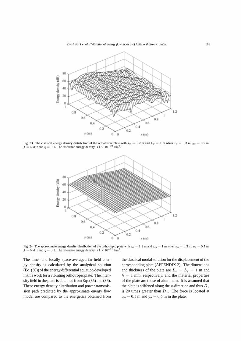
Fig. 23. The classical energy density distribution of the orthotropic plate withLx = 1.2 m andLy = 1 m whenxo = 0.3 m, yo = 0.7 m,f = 5 kHz andη = 0.1. The reference energy density is1 × 10−12 J/m2.
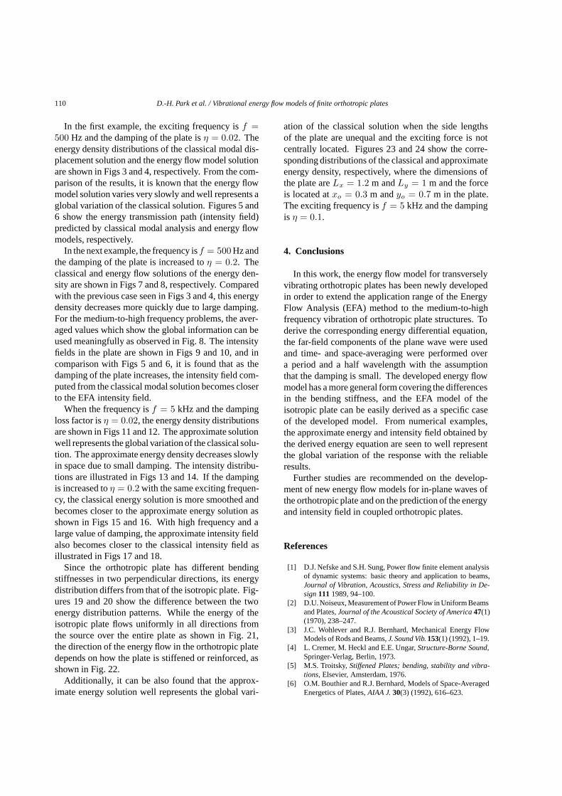
Fig. 24. The approximate energy density distribution of the orthotropic plate withLx = 1.2 m andLy = 1 m whenxo = 0.3 m, yo = 0.7 m,f = 5 kHz andη = 0.1. The reference energy density is1 × 10−12 J/m2.
The time- and locally space-averaged far-field ener-gy density is calculated by the analytical solution(Eq. (30)) of the energy differential equation developedin this work for a vibrating orthotropicplate. The inten-sity field in the plate is obtained from Eqs (35) and (36).These energy density distribution and power transmis-sion path predicted by the approximate energy flowmodel are compared to the energetics obtained from
the classical modal solution for the displacement of thecorresponding plate (APPENDIX 2). The dimensionsand thickness of the plate areLx = Ly = 1 m andh = 1 mm, respectively, and the material propertiesof the plate are those of aluminum. It is assumed thatthe plate is stiffened along they-direction and thusDy
is 20 times greater thanDx. The force is located atxo = 0.5 m andyo = 0.5 m in the plate.
110 D.-H. Park et al. / Vibrational energy flow models of finite orthotropic plates
In the first example, the exciting frequency isf =500 Hz and the damping of the plate isη = 0.02. Theenergy density distributions of the classical modal dis-placement solution and the energy flow model solutionare shown in Figs 3 and 4, respectively. From the com-parison of the results, it is known that the energy flowmodel solution varies very slowly and well represents aglobal variation of the classical solution. Figures 5 and6 show the energy transmission path (intensity field)predicted by classical modal analysis and energy flowmodels, respectively.
In the next example, the frequency isf = 500 Hz andthe damping of the plate is increased toη = 0.2. Theclassical and energy flow solutions of the energy den-sity are shown in Figs 7 and 8, respectively. Comparedwith the previous case seen in Figs 3 and 4, this energydensity decreases more quickly due to large damping.For the medium-to-high frequency problems, the aver-aged values which show the global information can beused meaningfully as observed in Fig. 8. The intensityfields in the plate are shown in Figs 9 and 10, and incomparison with Figs 5 and 6, it is found that as thedamping of the plate increases, the intensity field com-puted from the classical modal solution becomes closerto the EFA intensity field.
When the frequency isf = 5 kHz and the dampingloss factor isη = 0.02, the energy density distributionsare shown in Figs 11 and 12. The approximate solutionwell represents the global variation of the classical solu-tion. The approximate energy density decreases slowlyin space due to small damping. The intensity distribu-tions are illustrated in Figs 13 and 14. If the dampingis increased toη = 0.2 with the same exciting frequen-cy, the classical energy solution is more smoothed andbecomes closer to the approximate energy solution asshown in Figs 15 and 16. With high frequency and alarge value of damping, the approximate intensity fieldalso becomes closer to the classical intensity field asillustrated in Figs 17 and 18.
Since the orthotropic plate has different bendingstiffnesses in two perpendicular directions, its energydistribution differs from that of the isotropic plate. Fig-ures 19 and 20 show the difference between the twoenergy distribution patterns. While the energy of theisotropic plate flows uniformly in all directions fromthe source over the entire plate as shown in Fig. 21,the direction of the energy flow in the orthotropic platedepends on how the plate is stiffened or reinforced, asshown in Fig. 22.
Additionally, it can be also found that the approx-imate energy solution well represents the global vari-
ation of the classical solution when the side lengthsof the plate are unequal and the exciting force is notcentrally located. Figures 23 and 24 show the corre-sponding distributions of the classical and approximateenergy density, respectively, where the dimensions ofthe plate areLx = 1.2 m andLy = 1 m and the forceis located atxo = 0.3 m andyo = 0.7 m in the plate.The exciting frequency isf = 5 kHz and the dampingis η = 0.1.
4. Conclusions
In this work, the energy flow model for transverselyvibrating orthotropic plates has been newly developedin order to extend the application range of the EnergyFlow Analysis (EFA) method to the medium-to-highfrequency vibration of orthotropic plate structures. Toderive the corresponding energy differential equation,the far-field components of the plane wave were usedand time- and space-averaging were performed overa period and a half wavelength with the assumptionthat the damping is small. The developed energy flowmodel has a more general form covering the differencesin the bending stiffness, and the EFA model of theisotropic plate can be easily derived as a specific caseof the developed model. From numerical examples,the approximate energy and intensity field obtained bythe derived energy equation are seen to well representthe global variation of the response with the reliableresults.
Further studies are recommended on the develop-ment of new energy flow models for in-plane waves ofthe orthotropic plate and on the prediction of the energyand intensity field in coupled orthotropic plates.
References
[1] D.J. Nefske and S.H. Sung, Power flow finite element analysisof dynamic systems: basic theory and application to beams,Journal of Vibration, Acoustics, Stress and Reliability in De-sign 111 1989, 94–100.
[2] D.U. Noiseux, Measurement of Power Flow in Uniform Beamsand Plates,Journal of the Acoustical Society of America 47(1)(1970), 238–247.
[3] J.C. Wohlever and R.J. Bernhard, Mechanical Energy FlowModels of Rods and Beams,J. Sound Vib. 153(1) (1992), 1–19.
[4] L. Cremer, M. Heckl and E.E. Ungar,Structure-Borne Sound,Springer-Verlag, Berlin, 1973.
[5] M.S. Troitsky,Stiffened Plates; bending, stability and vibra-tions, Elsevier, Amsterdam, 1976.
[6] O.M. Bouthier and R.J. Bernhard, Models of Space-AveragedEnergetics of Plates,AIAA J. 30(3) (1992), 616–623.
D.-H. Park et al. / Vibrational energy flow models of finite orthotropic plates 111
[7] O.M. Bouthier and R.J. Bernhard, Simple Models of the En-ergetics of Transversely Vibrating Plates,J. Sound Vib. 182(1)(1995), 149–164.
[8] O.M. Bouthier, R.J. Bernhard and C. Wohlever, Energy andStructural Intensity Formulations of Beam and Plate Vibra-tions, 3rd International Congress on Intensity Techniques,1990, pp. 37–44.
[9] P.E. Cho, Energy Flow Analysis of Coupled Structures, Ph.D.Dissertation, Purdue University, 1993.
[10] R. Szilard,Theory and Analysis of Plates; classical and nu-merical methods, Prentice-Hall, Englewood Cliffs, 1974.
[11] S.A. Ambartsumyan,Theory of Anisotropic Plates; strength,stability and vibrations, Hemisphere Pub., New York, 1991.
[12] S. Timoshenko and W. Woinowski-Krieger,Theory of Platesand Shells, (2nd ed.), McGraw-Hill, New York, 1959.
[13] V.D. Belov, S.A. Rybak and B.D. Tartakovskii, Propagation ofVibrational Energy in Absorbing Structures,J. Soviet PhysicsAcoustics 23(2) (1977), 115–119.
Appendix 1. Space-average and omission of higherorder terms of damping loss factor
If Eq. (16) is expanded, the time-averaged total en-ergy density can be rewritten as
< e >=< e1 > + < e2 >,
where< e1 > and< e2 > are defined here by
< e1 > =14
Re{(Dxc|kx|4
+2√νxνy
√DxcDyck
2x(k2
y)∗
+2(1 −√
νxνy
)√DxcDyc|kx|2|ky|2
+Dyc|ky |4 +mω2)
× (|[A]−−|2 + |[B]+−|2
+|[C]−+|2 + |[D]|++|2)}and
< e2 >
=14
Re{(Dxc|kx|4
+2√νxνy
√DxcDyck
2x(k2
y)∗
+2(1 −√νxνy)
√DxcDyc|kx|2|ky|2
+Dyc|ky|4 +mω2) × ([A]−−([B]+−)∗
+[B]+−([A]−−)∗ + [A]−−([C]−+)∗
+[C]−+([A]−−)∗ + [A]−−([D]++)∗
+[D]++([A]−−)∗ + [B]+−([C]−+)∗
+[C]−+([B]+−)∗ + [B]+−([D]++)∗
+[D]++([B]+−)∗ + [C]−+([D]++)∗
+[D]++([C]−+)∗)
−2(1 −√νxνy)
√DxcDyc|kx|2|ky|2
([A]−−([B]+−)∗ + [B]+−([A]−−)∗
+[A]−−([C]−+)∗ + [C]−+([A]−−)∗
−[A]−−([D]++)∗ − [D]++([A]−−)∗
−[B]+−([C]−+)∗ − [C]−+([B]+−)∗
+[D]++([B]+−)∗ + [C]−+([D]++)∗
+[D]++([C]−+)∗).
Substituting the first above equation into Eq. (19)yields the time- and locally space-averaged total energydensity:
< e >=kxlkyl
π2
∫ π/kyl
0
∫ π/kxl
0
< e1 >
+ < e2 > dxdy
= < e1 > + < e2 > .
Then, if the damping of the plate is small, the expo-nential function in the right-hand side can be assumedto be nearly constant on the intervals of integration0 � x � (π/kxl) and0 � y � (π/kyl), the integralsfor the first unknown term|[A]−−|2 become:∫ π/kyl
0
∫ π/kxl
0
|A|2e−(η/2)kslx−(η/2)kylydxdy
≈ |A|2e−−∫ π/kyl
0
∫ π/kxl
0
dxdy
=π2
kxlkyl|A|2e−−.
Through the same process,< e1 > can be obtainedby
< e1 >=14
Re{Dxc|kx|4 + 2√νxνy
√DxcDyck
2x(k2
y)∗
+2(1 −√νxνy)
√DxcDyc|kx|2|ky|2
+Dyc|ky|4 +mω2}×(|A|2e−− + |B|2e+− + |C|2e−+ + |D|2e++).
The integrals for the unknown term[A]−−([B]+−)∗
can be obtained in the similar way:
112 D.-H. Park et al. / Vibrational energy flow models of finite orthotropic plates
∫ π/kyl
0
∫ π/kxl
0
[A]−−([B]+−)∗dxdy
= AB∗∫ π/kyl
0
e−(η/2)kyly
∫ π/kxl
0
e−2jkxlxdxdy
= AB∗∫ π/kyl
0
e−(η/2)kyly
e−2jkxlx
−2jkxl
∣∣∣∣x=π/kxl
x=0
dy
= 0.
As seen in the above equation,< e2 > is nullified,and the time- and locally space-averaged total energydensity< e > comes to be equal to< e1 >.
When the coefficient terms, Re{. . .}, are considered,they include high order terms of damping loss factorηas follows:
Re{Dxc|kx|4 + 2√νxνy
√DxcDyck
2x(k2
y)∗
+2(1 −√νxνy)
√DxcDyc|kx|2|ky|2
+Dyc|ky|4 +mω2}
=∣∣∣1 − j η
4
∣∣∣4 (Dxk4xl + 2
√νxνy
√DxDyk
2klk
2yl
+2(1 −√νxνy)
√DxDyk
2xlk
2yl
+Dyk4yl) +mω2
(1 +
η2
8+η4
256
)
(√Dxk
2xl +
√Dyk
2yl)
2 +mω2.
Neglecting all of the second and higher order termsof the damping loss factor with the dispersion relation(Eq. (6)), the time- and locally space-averaged totalenergy density< e > can be finally obtained as thesimplified Eq. (18).
Similarly, when spatially averaging the intensity(Eqs (14) and (15)) over a half wavelength, one canobtain the following expressions:
< qx >
=ω
2Re{kx(Dxck
2x +
√DxcDyck
2y)
+Dxc(k2x + νyk
2y)k∗x
+(1 −√νxνy)
√DxcDyckx|ky|2}
×(|A|2e−− − |B|2e+−
+|C|2e−+ − |D|2e++).
and
< qy >
=ω
2Re{ky(Dyck
2y +
√DxcDyck
2x)
+Dyc(k2y + νxk
2x)k∗y
+(1 −√νxνy)
√DxcDycky|kx|2}
×(|A|2e−− + |B|2e+−
−|C|2e−+ − |D|2e++).
The coefficient terms in the above equations havehigh order terms of damping loss factor that is assumedto be small:
Re{kx(Dxck2x +
√DxcDyck
2y)
+Dxc(k2x + νyk
2y)k∗x
+(1 −√νxνy)
√DxcDyckx|ky|2}
=(
1 − η2
16+η4
64
)kxl(Dxk
2xl +
√DxDyk
2yl)
+(
1 +716η2 − η4
64
)Dx(k2
xl + νyk2yl)kxl
+(
1 +516η2 +
η4
64
)kxl(1 −√
νxνy)
√DxDyk
2yl.
and
Re{ky(Dyck2y +
√DxcDyck
2x)
+Dyc(k2y + νxk
2x)k∗y
+(1 −√νxνy)
√DxcDycky|kx|2}
=(
1 − η2
16+η4
64
)kyl(Dyk
2yl +
√DxDyk
2xl)
+(
1 +716η2 − η4
64
)Dy(k2
yl + νxk2xl)kyl
+(
1 +516η2 +
η4
64
)kyl(1 −√
νxνy)
√DxDyk
2xl,
respectively. Here, neglecting all of the second andhigher order terms of the damping loss factor and usingthe dispersion relation (Eq. (6)) and Betti’s reciprocity
D.-H. Park et al. / Vibrational energy flow models of finite orthotropic plates 113
(νxDy = νyDx), the time- and locally space-averagedintensity components can be finally obtained as thesimplified Eqs (19) and (20).
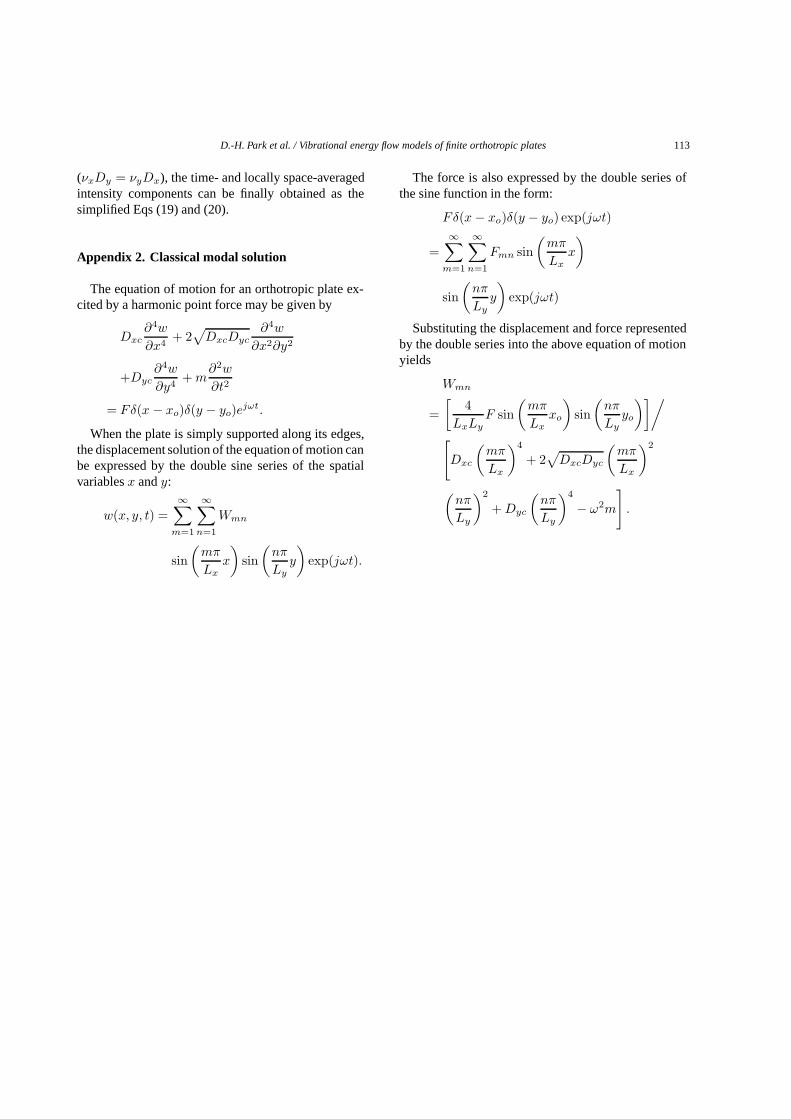
Appendix 2. Classical modal solution
The equation of motion for an orthotropic plate ex-cited by a harmonic point force may be given by
Dxc∂4w
∂x4+ 2√DxcDyc
∂4w
∂x2∂y2
+Dyc∂4w
∂y4+m
∂2w
∂t2
= Fδ(x − xo)δ(y − yo)ejωt.
When the plate is simply supported along its edges,the displacement solution of the equation of motion canbe expressed by the double sine series of the spatialvariablesx andy:
w(x, y, t) =∞∑
m=1
∞∑n=1
Wmn
sin(mπ
Lxx
)sin(nπ
Lyy
)exp(jωt).
The force is also expressed by the double series ofthe sine function in the form:
Fδ(x− xo)δ(y − yo) exp(jωt)
=∞∑
m=1
∞∑n=1
Fmn sin(mπ
Lxx
)
sin(nπ
Lyy
)exp(jωt)
Substituting the displacement and force representedby the double series into the above equation of motionyields
Wmn
=[
4LxLy
F sin(mπ
Lxxo
)sin(nπ
Lyyo
)]/[Dxc
(mπ
Lx
)4
+ 2√DxcDyc
(mπ
Lx
)2
(nπ
Ly
)2
+Dyc
(nπ
Ly
)4
− ω2m
].

International Journal of
AerospaceEngineeringHindawi Publishing Corporationhttp://www.hindawi.com Volume 2010
RoboticsJournal of
Hindawi Publishing Corporationhttp://www.hindawi.com Volume 2014
Hindawi Publishing Corporationhttp://www.hindawi.com Volume 2014
Active and Passive Electronic Components
Control Scienceand Engineering
Journal of
Hindawi Publishing Corporationhttp://www.hindawi.com Volume 2014
International Journal of
RotatingMachinery
Hindawi Publishing Corporationhttp://www.hindawi.com Volume 2014
Hindawi Publishing Corporation http://www.hindawi.com
Journal ofEngineeringVolume 2014
Submit your manuscripts athttp://www.hindawi.com
VLSI Design
Hindawi Publishing Corporationhttp://www.hindawi.com Volume 2014
Hindawi Publishing Corporationhttp://www.hindawi.com Volume 2014
Shock and Vibration
Hindawi Publishing Corporationhttp://www.hindawi.com Volume 2014
Civil EngineeringAdvances in
Acoustics and VibrationAdvances in
Hindawi Publishing Corporationhttp://www.hindawi.com Volume 2014
Hindawi Publishing Corporationhttp://www.hindawi.com Volume 2014
Electrical and Computer Engineering
Journal of
Advances inOptoElectronics
Hindawi Publishing Corporation http://www.hindawi.com
Volume 2014
The Scientific World JournalHindawi Publishing Corporation http://www.hindawi.com Volume 2014
SensorsJournal of
Hindawi Publishing Corporationhttp://www.hindawi.com Volume 2014
Modelling & Simulation in EngineeringHindawi Publishing Corporation http://www.hindawi.com Volume 2014
Hindawi Publishing Corporationhttp://www.hindawi.com Volume 2014
Chemical EngineeringInternational Journal of Antennas and
Propagation
International Journal of
Hindawi Publishing Corporationhttp://www.hindawi.com Volume 2014
Hindawi Publishing Corporationhttp://www.hindawi.com Volume 2014
Navigation and Observation
International Journal of
Hindawi Publishing Corporationhttp://www.hindawi.com Volume 2014
DistributedSensor Networks
International Journal of