Embed Size (px)
Citation preview

Quasinormal frequencies of self-dual black holes
Victor Santos,1, ∗ R. V. Maluf,1, † and C. A. S. Almeida1, ‡
1Universidade Federal do Ceará (UFC),
Departamento de Física, Campus do Pici,
Fortaleza - CE, C.P. 6030, 60455-760 - Brazil
(Dated: April 14, 2016)
AbstractOne simplified black hole model constructed from a semiclassical analysis of loop quantum gravity
(LQG) is called self-dual black hole. This black hole solution depends on a free dimensionless
parameter P known as the polymeric parameter and also on the a0 area related to the minimum
area gap of LQG. In the limit of P and a0 going to zero, the usual Schwarzschild-solution is
recovered. Here we investigate the quasinormal modes (QNMs) of massless scalar perturbations in
the self-dual black hole background. We compute the QN frequencies using the sixth order WKB
approximation method and compare them with numerical solutions of the Regge-Wheeler equation.
Our results show that as the parameter P grows, the real part of the QN frequencies suffers an
initial increase and then starts to decrease while the magnitude of the imaginary one decreases for
fixed area gap a0. This particular feature means that the damping of scalar perturbations in the
self-dual black hole spacetimes are slower, and their oscillations are faster or slower according to
the value of P .
PACS numbers: 04.70.Bw, 04.30.Nk, 04.60.Pp
∗ victor [email protected]† [email protected]‡ [email protected]
1
arX
iv:1
509.
0430
6v2
[gr
-qc]
12
Apr
201
6

I. INTRODUCTION
General relativity (GR) is an intrinsically nonlinear theory, where to derive useful quan-
tities from the field equations are difficult except for a few cases, for which usually there
are additional symmetries in the metric tensor. One fruitful approach is to consider the
weak-field approximation, leaving the field equations more treatable for many investigations
where the full equations are too difficult to solve. In particular, this approach led to the
prediction of Gravitational Waves (GWs).
The emission of gravitational waves can be associated with a variety of physical processes,
such as astrophysical phenomena involving the evolution of binary systems and stellar oscilla-
tions or cosmological processes that occurred in the very early universe [1]. Signals produced
by these processes have different intensities and characteristic frequencies. In general, their
spectral properties depend on the generating phenomenon [2].
Considerable progress has been made in the development of gravitational wave detectors.
Large ground-based gravitational wave interferometers, such as LIGO [3], GEO-600 [4],
TAMA-300 [5] and VIRGO [6] are increasing their detection rates, approaching then the
original design sensitivity [7]. These detections will provide useful information about the
composition of the astrophysical objects that generate them, like neutron stars. Moreover,
one of the most interesting aspects of the detection of gravitational waves is the connection
with black hole physics. The gravitational radiation emitted by an oscillating black hole
carry a fingerprint that may lead to a direct observation of its existence [8].
The investigation of the gravitational radiation from an oscillating star is usually done
by studying the perturbations of the stellar or black hole spacetimes. Such radiation ex-
hibits a certain set of characteristic frequencies, which are independent of the process that
generated it. These oscillation frequencies become complex due to the emission of gravita-
tional waves radiation, and the real and imaginary parts begin to represent the actual and
damping frequencies, respectively. Such characteristic oscillations are called quasinormal
modes (QNM). A striking feature of the QNM’s is that they are directly connected to the
parameters characterizing the black hole (mass, charge and angular momentum). The initial
studies on the black hole perturbations were carried out by Regge and Wheeler concerning
the stability of Schwarzschild black holes [9], followed by Zerilli [10, 11]. The QNM’s have
been found in perturbation calculations of particles falling into Schwarzschild and Kerr black
2
holes and in the collapse of a star to form a black hole [12, 13]. Numerical investigations of
the fully nonlinear equations of GR have provided results that agree with the perturbation
calculations [14–16].
The determination of QNM spectrum for real-world systems are very complicated once
that no analytical solutions are known for the relevant astrophysically systems, and, there-
fore, the investigation must proceed numerically. Additionally, the quasinormal frequencies
form a discrete set of points scattered on the complex plane, so that an exhaustive scan of
this plane is required to find the entire spectrum [17]. Furthermore, the QNM’s are known
to not form a complete set of functions, in the sense that a signal can not be written for all
times as a linear combination of these modes. A detailed account of quasinormal modes in
asymptotically flat spacetimes, their properties, and a discussion of its incompleteness can
be found in Refs. [18] and [15], and references therein.
In recent years, it has been suggested that the QNM’s of black holes might play a role
in quantum gravity, mainly in approaches like string theory and loop quantum gravity
(LQG). Indeed, it was proposed that the study of the black hole quasinormal modes in
anti-de Sitter spacetimes could be useful to determine properties of conformal field theories
in the context of the AdS-CFT correspondence [19]. However, such black hole solutions
can not describe astrophysical effects, since they are constructed in a negative cosmological
constant spacetime. In the context of loop quantum gravity, it was also suggested that the
large frequency limit for the QNM’s can be used to fix the Immirzi parameter, a parameter
measuring the quantum of area [20, 21]. Nevertheless, this is a fundamental issue that
remains open in this field. Inspired by these considerations, black hole quasinormal modes
have been computed in various background spacetimes, and in four or higher dimensions
[22, 23].
The semiclassical analysis of the full LQG black hole leads to an effective self-dual metric,
where the singularity is removed by replacing the singularity by an asymptotically flat region
[24]. As this effective metric recovers Schwarzschild metric as a limit, it is compelling
to investigate possible quantum modifications to already well-known effects discussed in
a classical Schwarzschild metric. For example, the study of the stability properties of the
Cauchy horizon in two different self-dual black hole solutions was carried out in Ref. [25]. In
Ref. [26] the authors studied the wave equation of a scalar field and calculated the particle
spectra of an evaporating self-dual black hole. Moreover, the thermodynamical properties
3

of self-dual black holes, using the Hamilton-Jacobi version of the tunneling formalism were
investigated in Refs. [27, 28].
The present work has as its main goal to examine the quasinormal mode frequencies of a
self-dual black hole, by taking a scalar field as a model of a gravitational wave. Although a
realistic scenario would require the computation of the frequencies for spin-2 perturbations,
scalar perturbations are a good starting point. They are simpler to study, and the grav-
itational field itself contains scalar degrees of freedom [9], providing a qualitative similar
analysis. We computed the frequencies employing a 3rd-order and 6th-order WKB approxi-
mation, comparing them with previous calculations in the classical limit. We also solved the
full Regge-Wheeler equation in the time domain, comparing the semianalytic frequencies as
a fit for the time profile. We found that the polymeric parameter P induces a more slowly
decay for the scalar field while its oscillation becomes higher or lower according to the value
of P .
The paper is structured as follows. We introduce self-dual black hole solution in section
II. In section III we compute the self-dual black hole quasinormal frequencies, exhibiting
the time-domain profile and finally we summarize the work and present our final remarks in
section IV.
II. SELF-DUAL BLACK HOLE
Loop Quantum Gravity [29–31] provided a description of the universe in its early stages.
One key feature is the resolution of initial singularity [32, 33], where the Big Bang singularity
is replaced by a quantum bounce. A black hole in this framework was constructed from a
modification of the holonomic version of the Hamiltonian constraint [24]. This kind of black
hole, called self-dual black hole, has a solution which depends on a parameter δ, called
polymeric parameter, which labels elements in a class of Hamiltonian constraints. These
constraints are compatible with spherical symmetry and homogeneity, and they can be
uniquely fixed from asymptotic boudary conditions, yielding the proper classical Hamiltonian
in the limit δ → 0.
Following the approach of Refs. [25, 26], the loop quantum corrected Schwarzschild black
4
hole can be described by the effective metric
ds2 = −F (r)dt2 +dr2
G(r)+H(r)dΩ2
2, (1)
where dΩ22 = dθ2 + sin2 θdφ2 and the metric functions are given by
F (r) =(r − r+)(r − r−)(r + r∗)
2
r4 + a20, (2)
G(r) =(r − r+)(r − r−)r4
(r + r∗)2(r4 + a20), (3)
H(r) =a20r2
+ r2, (4)
with r+ = 2m, r− = 2mP 2, r∗ = 2mP . The parameter m is related to the ADM mass M by
M = m(1 + P )2. Moreover, the function P is called polymeric function, and it is related to
the polymeric parameter δ by P (δ) = (√
1 + γ2δ2 − 1)/(√
1 + γ2δ2 + 1), where γ denotes
the Barbero-Immirzi parameter. The area gap a0 equals to Amin/8π, with Amin being the
minimum area of LQG, namely
Amin = 8π`2Pγ√jmin(jmin + 1), (5)
where `P is the Planck length and jmin is the smallest value of the representation on the
edge of the spin network crossing a surface. A common choice is to consider representations
of the SU(2) group, which leads to jmin = 1/2 and then a0 = γ√
3`2P/2. In this work we will
assume γ ∼ 1, so that we fix a0 =√
3/2 in Planck units.
The self-duality property can be expressed by saying that the metric (1) is invariant under
the transformations
r → a0/r, t→ tr2∗/a0, r± → a0/r∓. (6)
The minimal surface element is obtained when the dual coordinate r = a0/r takes the value
rdual = r =√a0. The property of self-duality removes the black hole singularity by replacing
it with another asymptotically flat region. For the dynamical aspects of this solution we
refer the reader to Ref. [26]. However, the polymerization of the Hamiltonian constraint
in the homogeneous region is inside the event horizon. Therefore, the physical meaning of
the solution when the metric is analytically continued to all spacetime persist as an open
problem [25]. Moreover, self-dual black holes have two horizons – an event horizon and a
Cauchy horizon. Cauchy horizons are unstable, and then it is not clear whether the solution
5

has a stable interior. Nevertheless, this solution can be useful as a first approximation to the
behavior of a system in a quantum gravitational framework. One advantage of this approach
is that although the full black hole solution can only be presented in a numerical form, this
solution has a closed form which makes our investigation easier.
Concerning the experimental bound of the polymerization parameter, a recent study
based on observation of solar gravitational deflection of radio waves leads to the constraint
[34]
δ . 0.1 (7)
for the polymerization parameter, which implies P ∼ 10−3. We stress that this estimate
has as asumption γ < 0.25, and since we did a different choice for the value of the Barbero-
Immirzi parameter we will therefore impose a less restrictive range of values P < 1.
III. QUASINORMAL FREQUENCIES
In this section we are interested in obtaining the solutions of wave equations in the
presence of a background spacetime described by (1), and thus to find the QNM frequencies.
In most cases it is not feasible to solve the wave equations and find frequencies exactly.
Among the analytical methods used in literature, the WKB method is one of the most
popular. The WKB method was first used by Iyer and Will [35, 36], and later improved to
sixth order by Konoplya [22].
Now, we consider the behavior of a scalar field in a self-dual black hole background. The
propagation of a massless scalar field is described by the Klein-Gordon equation in curved
space-time1√−g
∂µ(gµν√−g∂νΦ
)= 0, (8)
where the field is treated as an external perturbation. In other words, we ignore the backre-
action. Spherical symmetry allow us to decompose the field in terms of spherical harmonics,
Φ(t, r, θ, ϕ) =∞∑`=0
∑m=−`
1√H(r)
Ψ`,m(t, r)Y`,m(θ, ϕ), (9)
and substituting Eq. (9) into Eq. (8) one can find the radial coefficients which satisfy the
equation
− ∂2Ψ
∂t2+∂2Ψ
∂x2+ V (x)Ψ = 0, (10)
6

where we introduced the tortoise coordinate x, defined by
dxdr
=r4 + a20
r2(r − r−)(r − r+). (11)
After integrating, the tortoise coordinate assumes the explicit form
x = r − a20rr−r+
−(a20 + r4−
)log |r − r−|
r2− (r+ − r−)
+
(a20 + r4+
)log |r − r+|
r2+ (r+ − r−)+a20 (r− + r+) log(r)
r2−r2+
, (12)
such that x→ ±∞ for r → r∓. The function V (x) is called Regge-Wheeler potential, and it
encodes the information regarding the black hole geometry. To the present case it is given
by [25]
V (r(x)) =(r − r−)(r − r+)
(r4 + a20)4
[r2(a40(r( (K2 − 2
)r + r− + r+
)+ 2K2rr∗ +K2r2∗
)+ 2a20r
4( (K2 + 5
)r2 + 2K2rr∗ +K2r2∗ − 5r(r− + r+) + 5r−r+
)+ r8
(K2(r + r∗)
2 + r(r− + r+)− 2r−r+) )]
, (13)
with K2 = `(`+ 1). From this expression, we note that V (x) vanishes at r = r− and r = r+,
and as discussed in Ref. [25], the maximum of the potential occurs at r ≈ `P/3.
We will now look for stationary solutions in the form Ψ ∼ ψ(r)e−iωt. With this ansatz,
equation (10) takes the form of a Schrödinger equation given by
∂2ψ
∂x2−[ω2 − V (x)
]ψ = 0. (14)
Before solving Eq. (14), we must state the boundary conditions. Since we are dealing with
a black hole geometry, physically acceptable solutions are purely ingoing near the horizon
in the form
ψin(r) ∼
e−iωx (x→ −∞)
C(−)` (ω)e−iωx + C
(+)` (ω)eiωx (x→ +∞),
(15)
where C(−)` (ω) and C(+)
` (ω) are complex constants that depend on the variables ` and ω.
QNMs of black holes are in general defined as the set of frequencies ω`n such that
C(−)` (ω`n) = 0, i.e., which are associated with purely outgoing wave at the spatial infinity
and purely ingoing wave at the event horizon. Here the ` and n labels are integers, called
multipole and overtone numbers respectively. Since the spectrum of QNMs is in fact de-
termined by the eigenvalues of the equation (14), it is convenient to promote the analogy
7

with quantum mechanics and make use of semianalytical methods. Next, we will employ a
high-order WKB approach to calculating the QNM frequencies for some values of ` and n
indexes.
A. WKB analysis
The WKB approximation method to evaluate the QNMs was first implemented by Schutz
and Will in the calculation of the particles scattering around black holes [16]. An improve-
ment in the method up to sixth WKB order has been given by Konoplya [22, 23]. The
method can be applied if the potential has the form of a barrier, going to constant values
when x→ ±∞. At each limit, the frequencies are calculated by matching the power series
of the solution near the maximum of the potential through its turning points.
In the general case, Konoplya’s WKB formula to the QN frequencies can be written as
i(ω2n − V0)√−2V ′′0
−6∑i=2
Λi = n+1
2, (16)
where V ′′0 is the second derivative of the potential on the maximum r0 and Λi are constant
coefficients which depend on the effective potential and its derivatives (up to 12-th order)
at the maximum.
Table I. Quasinormal modes computed using 3rd-order WKB approximation, for different values of
the polymerization parameter. The multipole number is fixed to ` = 1.
P ω0 ω1 ω2
0.1 0.3031− 0.0981i 0.2704− 0.3079i 0.2249− 0.5293i
0.2 0.3174− 0.0971i 0.2887− 0.3030i 0.2487− 0.5195i
0.3 0.3291− 0.0944i 0.3047− 0.2928i 0.2706− 0.5006i
0.4 0.3376− 0.0900i 0.3176− 0.2775i 0.2891− 0.4730i
0.5 0.3421− 0.0839i 0.3260− 0.2573i 0.3028− 0.4374i
0.6 0.3417− 0.0763i 0.3288− 0.2330i 0.3095− 0.3950i
0.7 0.3355− 0.0677i 0.3246− 0.2058i 0.3071− 0.3483i
0.8 0.3227− 0.0587i 0.3121− 0.1783i 0.2940− 0.3016i
In tables I and II we present the tabulated quasinormal frequencies using respectively the
3-rd and 6-th order WKB method for a fixed multipole ` = 1. Some comments are in order.
8
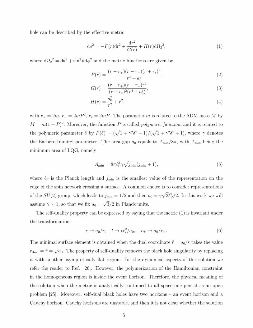
Table II. Quasinormal modes computed using 6th-order WKB approximation, for different values
of the polymerization parameter. The multipole number is fixed to ` = 1.
P ω0 ω1 ω2
0.1 0.3056− 0.0983i 0.2770− 0.3073i 0.2399− 0.5401i
0.2 0.3194− 0.0973i 0.2940− 0.3025i 0.2606− 0.5283i
0.3 0.3307− 0.0946i 0.3088− 0.2924i 0.2796− 0.5073i
0.4 0.3388− 0.0901i 0.3204− 0.2771i 0.2951− 0.4784i
0.5 0.3430− 0.0839i 0.3283− 0.2568i 0.3073− 0.4400i
0.6 0.3424− 0.0763i 0.3309− 0.2323i 0.3139− 0.3944i
0.7 0.3358− 0.0677i 0.3244− 0.2063i 0.3026− 0.3558i
0.8 0.3233− 0.0587i 0.3156− 0.1764i 0.3061− 0.2903i
First, the QN frequencies associated with the scalar field have a negative imaginary part;
this means that the QNMs decay exponentially in time, losing energy in the form of scalar
waves. This result was already expected and has also been found for scalar, electromagnetic
and gravitational perturbations in the Schwarzschild-like geometry [37]. They also have a
similar behavior to the usual case (P → 0 and a0 → 0) regarding the overtone number scale,
so that the real part decreases, whereas the magnitude of imaginary one grows for crescent
values of overtone number n. Our main result concerns the behavior of QN frequencies with
respect to the polymeric parameter P . We note that the real part of the QN frequencies
begins to grow and then decreases as P increases, while the magnitude of the imaginary
part decreases. This means that as the polymerization parameter gets larger the frequency
of the massless scalar wave shift higher or lower, and it has a slower damping.
It is interesting to plot the frequencies in the complex plane in contrast with the frequen-
cies of the Schwarzschild case. In figure 1 this is done considering three families of multipoles
` = 0, 1, 2 for the Schwarzschild case. We can notice the deviation from the classical case as
we increase the polymerization function. Looking at the right side of the figure, we conclude
that the frequency curves are moving counterclockwise as P grows, and this twisting effect
becomes more apparent for larger values of the angular quantum number `. Furthermore,
these results differ from the frequencies found in Ref. [38], where a quantum correction was
introduced as a deformation as introduced in Ref. [39].
9

Figure 1. Scalar field normal modes. The markers denote the multipole number as: ` = 0 (circle),
` = 1 (square), ` = 2 (triangle), while the colors denote the value of the polymerization parameter:
P = 0.1 (blue), P = 0.2 (green), P = 0.3 (orange), P = 0.6 (red). The black markers denote the
frequencies for the Schwarzschild black hole.
The 6th-order WKB formula usually provides a better approximation than the 3rd-order
formula. Since the WKB series converges only asymptotically, in general we can not guar-
antee the convergence only by increasing the WKB order. In Fig. 2 we present the real and
imaginary parts of the frequencies as a function of the WKB order for fixed multipole and
overtone, respectively ` = 0 and n = 0. From this we can observe that indeed both real
and imaginary parts converge as we increase the order, evidencing the effectiveness of the
method.
The presented results one show that the real part of the quasinormal frequencies first
increase and then start to decrease with the polymerization parameter, meaning a shift
from blue to red into the spectrum of the massless scalar wave function. The magnitude of
the imaginary part decreases with P , meaning a slower damping than of the classical result.
The conclusion is that loop quantum black holes decay slower than its classical analogue.
In this context, we expect that this is caused by the domination of curvature effects in the
10

Figure 2. Real (blue/top) and imaginary (red/bottom) parts of the quasinormal frequencies as
a function of the WKB order for the ` = 0, n = 0 mode, for some values of the polymerization
parameter P .
quantum regime.
B. Time-domain solution
Due to the complex form of the effective potential, in order to contemplate the role of the
QN spectrum in a time-dependent scattering we will investigate the scalar perturbations in
the time domain. For this we employ the characteristic integration method developed by
Gundlach and collaborators [14]. This method uses light-cone coordinates u = t − x and
v = t+ x, in a way the wave equation can be recasted as(4∂2
∂u∂v+ V (u, v)
)Ψ(u, v) = 0. (17)
Equation (17) can be integrated numerically by a simple finite-difference method, using
the discretization scheme
Ψ(N) = −Ψ(S) + Ψ(W ) + Ψ(E)− h2
8V (S)
[Ψ(W ) + Ψ(E)
]+ O(h4), (18)
11

where S = (u, v), W = (u+h, v), E = (u, v+h), N = (u+h, v+h) and h is an overall grid
scale factor.
The initial data are specified at null surfaces u = u0 and v = v0. We chose a Gaussian
profile centered at v = vc and width σ on u = u0,
Ψ(u = u0, v) = Ae−(v−v∗)2/(2σ2), Ψ(u, v0) = Ψ0, (19)
and at v = v0 we posed a constant initial condition: Ψ(u, v0) = Ψ0. We can choose without
loss of generality Ψ0 = 0. Once chosen the null data, integration proceeds at u = const.
lines in the direction of increasing v.
(a) ` = 0. (b) ` = 1.
(c) ` = 2.
Figure 3. Log-log plots of the time domain profiles for the scalar perturbations at x = 10M , for
several values of the polymerization parameter P .
We now report our results for the scalar test field. We setm = 1 without loss of generality,
and we chose as null data a Gaussian profile with width σ = 3.0 centered at u = 10 at the
12

surface u = 0, and Ψ0 = 0. The grid was chosen to be u ∈ [0, 1000] and v ∈ [0, 1000], with
points sampled in such a way we have the overall grid factor h = 0.1.
Figures 3(a), 3(b), and 3(c) show the typical evolution profiles, in comparison with that of
the classical Schwarzschild black hole. The classical result is visually indistinguishable from
the profile P = 0.001, which is consistent with the fact that P → 0 corresponds to a classical
profile. We can observe the domination of damped oscillations (quasinormal ringing) in the
region v ∼ 200, before a power-law tail takes over in later times. As we consider larger
multipole numbers, we observe a discrepancy between the quantum and classical results.
indeed, with ` = 2 the curve P = 0.001 (Fig. 3(c)) seems to have a larger oscillation even
during the tail, while the other curves started to be dominated by the power-law tail. This
is still consistent with the conclusion obtained from the analysis of the WKB spectrum
presented in Sec. III A, since althought we took a small value for P we should still consider
the fluctuations due to the area gap a0 in the scattering potential.
Figure 4. Numerical evolution of waveform (solid line) for ` = 0 and the fit from the 6-th-order
WKB frequencies, for several values of the polymerization parameter. For the fit we took the
fundamental mode and the first overtone.
In Figs. 4 and 5, we compared the time-domain solutions with a solution constructed
from a linear combination of plane waves whose frequencies are given by the WKB method
estimates. We considered a linear combination of the fundamental mode and the first over-
13
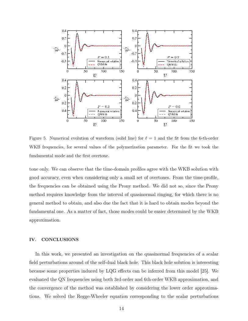
Figure 5. Numerical evolution of waveform (solid line) for ` = 1 and the fit from the 6-th-order
WKB frequencies, for several values of the polymerization parameter. For the fit we took the
fundamental mode and the first overtone.
tone only. We can observe that the time-domain profiles agree with the WKB solution with
good accuracy, even when considering only a small set of overtones. From the time-profile,
the frequencies can be obtained using the Prony method. We did not so, since the Prony
method requires knowledge from the interval of quasinormal ringing, for which there is no
general method to obtain, and also due the fact that it is hard to obtain modes beyond the
fundamental one. As a matter of fact, those modes could be easier determined by the WKB
approximation.
IV. CONCLUSIONS
In this work, we presented an investigation on the quasinormal frequencies of a scalar
field perturbations around of the self-dual black hole. This black hole solution is interesting
because some properties induced by LQG effects can be inferred from this model [25]. We
evaluated the QN frequencies using both 3rd-order and 6th-order WKB approximation, and
the convergence of the method was established by considering the lower order approxima-
tions. We solved the Regge-Wheeler equation corresponding to the scalar perturbations
14

around the black hole, verifying the agreement with the QNM frequencies from the WKB
method.
The computed frequencies implied a slower decaying rate for black holes in quantum
regime. This behaviour has been shown to be sensitive to the polymerization parameter
and to the area gap, converging to the classical behavior when these parameters vanishes.
We hope this could give clues about the evaporation process of quantum black holes at
qualitative level.
We emphasize that our analysis has the limitation that the metric used does not corre-
spond to the full LQG solution. Also, we considered only scalar perturbations. In a more
realistic scenario one should treat gravitational (tensorial) perturbations as well. However
QNMs from scalar perturbations of variations of non-charged, non-spinning black holes are
widely studied in the literature and the QNMs found here are able to be compared with
those arising in these other models. Furthermore, the qualitative relationship we have found
is expected to carry over to realistic, astrophysical black holes.
ACKNOWLEDGMENTS
This work was partially supported by the Brazilian agencies Coordenação de Aperfeiçoa-
mento de Pessoal de Nível Superior (CAPES) and Conselho Nacional de Desenvolvimento
Científico e Tecnológico (CNPq). Victor Santos would like to thank R. Konoplya for pro-
viding the WKB correction coefficients in electronic form. He also would like to thank Prof.
Abhay Ashtekar for the kind hospitality at Institute of Gravitation and Cosmos of The
Pennsylvania State University, where part of this work was done.
[1] B. Sathyaprakash and B. F. Schutz, Living Reviews in Relativity 12 (2009), 10.12942/lrr-2009-
2.
[2] K. Riles, Progress in Particle and Nuclear Physics 68, 1 (2013).
[3] A. Abramovici, W. E. Althouse, R. W. P. Drever, Y. Gürsel, S. Kawamura, F. J. Raab,
D. Shoemaker, L. Sievers, R. E. Spero, K. S. Thorne, R. E. Vogt, R. Weiss, S. E. Whitcomb,
and M. E. Zucker, Science 256, 325 (1992).
[4] H. Lück and the GEO600 Team, Classical and Quantum Gravity 14, 1471 (1997).
15

[5] E. Coccia, G. Pizzella, and F. Ronga, eds., Gravitational Wave Experiments, Proceedings of
the First Edoardo Amaldi Conference, Vol. 1 (1994).
[6] V. Fafone, “Advanced virgo: an update,” in The Thirteenth Marcel Grossmann Meeting (World
Scientific, 2015) Chap. 347, pp. 2025–2028.
[7] M. Evans, General Relativity and Gravitation 46, 1778 (2014).
[8] K. S. Thorne, arXiv:gr-qc/9706079 (1997), arXiv: gr-qc/9706079.
[9] T. Regge and J. A. Wheeler, Phys. Rev. 108, 1063 (1957).
[10] F. J. Zerilli, Phys. Rev. D 2, 2141 (1970).
[11] F. J. Zerilli, Phys. Rev. D 9, 860 (1974).
[12] L. Motl and A. Neitzke, Adv.Theor.Math.Phys. 7, 307 (2003).
[13] H.-P. Nollert and B. G. Schmidt, Phys. Rev. D 45, 2617 (1992).
[14] C. Gundlach, R. H. Price, and J. Pullin, Phys. Rev. D 49, 883 (1994), 00282.
[15] H.-P. Nollert, Classical and Quantum Gravity 16, R159 (1999).
[16] B. F. Schutz and C. M. Will, The Astrophysical Journal 291, L33 (1985), 00266.
[17] J. L. Blazquez-Salcedo, L. M. Gonzalez-Romero, and F. Navarro-Lerida, Phys. Rev. D87,
104042 (2013), arXiv:1207.4651 [gr-qc].
[18] K. D. Kokkotas and B. G. Schmidt, Living Reviews in Relativity (1999).
[19] G. T. Horowitz and V. E. Hubeny, Phys. Rev. D 62, 024027 (2000).
[20] O. Dreyer, Phys. Rev. Lett. 90, 081301 (2003).
[21] L. Motl, Adv.Theor.Math.Phys. 6, 1135 (2003).
[22] R. A. Konoplya, Journal of Physical Studies 8, 93 (2004).
[23] R. A. Konoplya, Physical Review D 68 (2003).
[24] L. Modesto and I. Prémont-Schwarz, Physical Review D 80 (2009).
[25] E. Brown, R. Mann, and L. Modesto, Physics Letters B 695, 376 (2011).
[26] S. Hossenfelder, L. Modesto, and I. Prémont-Schwarz, (2012), arXiv:1202.0412 [gr-qc].
[27] C. Silva and F. Brito, Physics Letters B 725, 456 (2013).
[28] M. Anacleto, F. Brito, and E. Passos, Physics Letters B 749, 181 (2015).
[29] A. Ashtekar and J. Lewandowski, Classical and Quantum Gravity 21, R53 (2004).
[30] M. Han, Y. Ma, and W. Huang, International Journal of Modern Physics D 16, 1397 (2007).
[31] T. Thiemann and H. Kastrup, Nucl.Phys. B399, 211 (1993).
[32] A. Ashtekar, Gen. Rel. Grav. 41, 707 (2009).
16

[33] M. Bojowald and H. A. Morales-Tecotl, Lect.Notes Phys. 646, 421 (2004).
[34] S. Sahu, K. Lochan, and D. Narasimha, Phys. Rev. D 91, 063001 (2015).
[35] S. Iyer and C. M. Will, Physical Review D 35, 3621 (1987), 00298.
[36] S. Iyer, Phys. Rev. D 35, 3632 (1987).
[37] R. A. Konoplya and A. Zhidenko, Rev. Mod. Phys. 83, 793 (2011), arXiv:1102.4014 [gr-qc].
[38] M. Saleh, B. B. Thomas, and T. C. Kofane, Astrophysics and Space Science 350, 721 (2014).
[39] D. Kazakov and S. Solodukhin, Nuclear Physics B 429, 153 (1994).
17