VictorLazzariniandJosephTimoney NewPerspectiveson ...eprints.maynoothuniversity.ie/4104/1/VL_New_perspectives.pdf · NewPerspectiveson DistortionSynthesisfor VirtualAnalogOscillators

New Perspectives onDistortion Synthesis forVirtual Analog Oscillators

Victor Lazzarini and Joseph TimoneyAn Grupa Theicneolaıocht Fuaime agusCeoil Dhigitigh(Sound and Digital Music TechnologyGroup)National University of Ireland, MaynoothMaynooth, Co. Kildare, [email protected]@cs.nuim.ie

The term “virtual analog” (VA) first appeared in the1990s with the commercial introduction of digitalsynthesizer instruments that were intended toemulate the earlier analog subtractive synthesizers,such as those produced by, among others, Moogor Sequential Circuits (Smith 2008). In creating a“virtual analog” digital model, two approaches arepossible: the first is to build an explicit digital modelderived from the various electrical components thatform the original analog circuit; the second is touse digital processing structures that will produceoutputs that mimic those of the analog system. Todate, the second approach has been used for theimplementation of the elements of virtual analogsubtractive synthesizers, as real-time computationalconstraints limit the efficacy of circuit models inusable software instruments (Civolani and Fontana2008). Among the features of a subtractive synthesissystem, one aspect that has received more attentionthan others is algorithms for real-time digitalgeneration of the periodic waveforms associatedwith voltage-controlled oscillators (VCO), such assawtooths, square waves, and triangle waves, alsoknown as the classic analog waveforms (Stilson2006).

Although the original analog waveforms theoreti-cally had an infinite bandwidth, the digital versionsmust be bandlimited to half the sampling frequency(Stilson 2006). If this is not the case, the audio outputcan exhibit excessive aliasing distortion, which canseverely corrupt the sound quality. This distortionis manifested as audio disturbances that includeinharmonicity, beating, and heterodyning. It can beparticularly severe when the ratio of the waveformfundamental frequency to the sampling frequency isnot an integer, as the aliased components will thenfall in between the signal harmonics (Valimaki and

Computer Music Journal, 34:1, pp. 28–40, Spring 2010c© 2010 Massachusetts Institute of Technology.

Huovilainen 2007). Furthermore, although a crudetechnique such as using oversampling with a trivialwaveform generator followed by downsampling tothe audio rate afterwards can help to amelioratesome of the distortion (Chamberlain 1987), thedrawback is that this adds significantly to the com-putational cost of the implementation. This thenimpacts on other synthesizer features such as thepermissible degree of polyphony. Therefore, for VAsubtractive synthesizers, a key goal currently is todevelop algorithms that can generate bandlimiteddigital versions of the classic periodic waveforms ata low computational cost.

To date, a number of algorithms have been pro-posed for the production of bandlimited digitalperiodic waveforms. However, even though thevariety of approaches appears diverse (Valimaki andHuovilainen 2007), in fact they can be unified inthat all can be shown to be connected to nonlineardistortion synthesis (Dodge and Jerse 1985). Perhapsone of the most important discoveries of early digitalsound synthesis, distortion-based methods domi-nated the research landscape of computer music inthe 1970s and 1980s. A framework for these tech-niques was developed through the pioneering workof John Chowning on frequency modulation (FM)synthesis (Chowning 1973); Godfrey Winham, KenSteiglitz, and Andy Moorer on discrete summationformulae (DSF; Winham and Steiglitz 1970; Moorer1976, 1977); and Daniel Arfib and Marc LeBrunon digital waveshaping (Arfib 1978; LeBrun 1979).These techniques were demonstrated to stem fromthe same principles and to have interchangeableinterpretations. Perhaps the key aspect that madethem so interesting in the early days of computermusic was their low computational cost. A num-ber of variants, especially of FM synthesis, werekeenly explored (e.g., Schottstaedt 1977; Palamin,Palamin, and Ronveaux 1988; Chowning 1989). Inthe 1990s, interest in these techniques diminished,

28 Computer Music Journal

even though some important novel methods werestill being proposed, such as that of Puckette (1995).More recently, distortion techniques have been usedin new synthesis algorithms (Lazzarini, Timoney,and Lysaght 2008b) and for audio effects (Lazzarini,Timoney, and Lysaght 2007, 2008a, 2008c).

The development of research into VA oscillatormodels has somewhat rekindled the interest intechniques that can be interpreted from a nonlineardistortion perspective. However, the literature hasso far been limited in terms of discussing these newmethods from that angle. In the following discus-sion, we hope to address this issue and propose newnonlinear distortion synthesis algorithms for classicanalog-waveform generation. Such signals are nor-mally represented by the sawtooth wave (containingall harmonics with 1/n weights, n being the har-monic number), the square wave (all odd harmonics,1/n), and the triangle (all odd harmonics, 1/n2).

Distortion Synthesis and Analog Waveform Models

We now present a brief survey of key methodsmethods for the digital generation of the classicperiodic waveforms of subtractive synthesis. Ouraim is to show how these fall within the frameworkof nonlinear distortion synthesis, demonstrating itspotential for further designs.

Lane’s Analog Model Oscillator

The technique of nonlinear waveshaping is thebasis for one of the early VA models of oscillators(Lane et al. 1997). The algorithm is based on theuse of the modulus and absolute-value functionsfollowed by filtering to suppress the aliased portionsof the spectrum and correct the spectral rolloff. Thewaveshaping expression is, with ω = 2π ft, given by

x(t) = f(sin

(ω

2

))= abs

(sin

(ω

2

))(1)

The spectrum of such a waveshaped signal is notbandlimited, but the most objectionable aliasedcomponents in the vicinity of half the samplingrate are reduced by a low-pass filter. Theoretically,the waveshaper output will contain all components

from ω upwards, in decreasing strength, plus acertain amount of DC energy (Lane et al. 1997):

x(t) = 2[

1π

− 2π

(cos(ω)

1.3+ cos(2ω)

3.5+ cos(3ω)

5.7+ · · ·

)]

(2)

By using an adaptive high-pass filter, the steeperrolloff can be corrected to yield an approximate saw-tooth spectrum. If we generate a second sawtooth-like wave at ω/2 and subtract it from the originalsignal, then square and triangle wave approxima-tions are obtained. This method seems to providean efficient algorithm for the digital generation ofsubtractive synthesis oscillator waveforms, but withsome aliasing penalty.

Differentiated Parabolic Wave

Differentiated parabolic wave (DPW) synthesis(Valimaki 2005; Valimaki and Huovilainen 2006,2007) can be described in terms of nonlinear distor-tion, as it is based on a parabolic waveshaping of anon-bandlimited sawtooth wave. Similarly to themethod in the previous section, the DPW methodis also a non-bandlimited but alias-suppressed algo-rithm. Instead of starting with a sinusoidal signal,the function mapping here uses a complex, alreadyaliased input generated by a modulo counter, whichis for all practical purposes a non-bandlimited saw-tooth wave. Following on from the waveshapingprocess, a high-pass filter (a first-order difference) isused to approximate a sawtooth shape. This methodseems to provide an efficient algorithm for VAoscillators, but with some aliasing penalty.

Band-Limited Impulse Train and DiscreteSummation Formulae

DSF and band-limited impulse train (BLIT; Stilsonand Smith 1996) are similar techniques. In fact,the sinc-based BLIT and the original Winham andSteiglitz DSF pulse are effectively two ways ofexpressing the same closed-form summation. Bothof these methods fall within the nonlinear distortionframework. Moorer’s DSF algorithm in particular

Lazzarini and Timoney 29

can have an interesting re-casting as a waveshapingprocess (LeBrun 1979), where one of its four originalformulae,

s(t) =∞∑

n=1

an cos(nω) = 1 − a cos(ω)1 + a2 − 2a cos(ω)

(3)

can be reinterpreted as a cosine wave mapped by atransfer function,

f (x) = 1 − ax1 + a2 − 2ax

(4)

This fact demonstrates some interesting points ofconnections between waveshaping and summation-formulae methods. DSF is also strongly connectedwith FM synthesis, as the latter can be seen as aclosed-form summation formula (Dodge and Jerse1985).

Phase Distortion or Phaseshaping

The technique of phase distortion (PD), imple-mented in the Casio CZ series of synthesizers(Massey, Noyes, and Shklair 1987; Roads 1996),has been somewhat ignored in the literature eventhough it has been shown to be a means of digitallygenerating the classic periodic waveforms of subtrac-tive synthesis (Ishibashi 1987). Because this methodhas escaped a more formal treatment, we will tryto sketch some of its main points in the followingdiscussion. In addition, we will propose some newalternative approaches to its implementation.

The main technical reference for it is a patent(Ishibashi 1987) where the basic method is described.PD is, effectively, complex frequency or phasemodulation in disguise. Using a sinusoidal oscillator,the output signal is produced by using a nonlinearphase increment,

spd(t) = − cos(φpd(t)) (5)

where φpd(t) is our distorted phase increment. (Here,we use –cos() to keep the original formulation asper Ishibashi (1987) in line with our convention ofunipolar 2π -modulo phase.) The phase is in factmade up of a linear increment φ(t) and a modulation

Figure 1. Phase-distortionsynthesis, original design(solid line). A 50-harmonicbandlimited sawtooth isplotted as comparison(dotted line).

function mdpd(t):

φpd(t) = φ(t) + mdpd(t) (6)

We can see in Figure 1 that the function shape is asmooth version of a trivial sawtooth wave, and thusit should have lower energy in its higher frequencieswith a consequent reduction in aliasing. One of theproblems is that, given the straight angles of themodulating function, we will not be able to producea strictly bandlimited output, and some aliasingmay occur. In practice, by limiting the amount ofdistortion, it is possible to reduce the foldover toacceptable levels.

Another solution is, of course, to try to producea roughly bandlimited phase distortion, either bypolynomial or Fourier-series approximation of themodulation function. In fact, we can see in Figure 1that the function shape is very close to that ofa bandlimited sawtooth. Because we know howto describe PD synthesis as complex FM (LeBrun1977), we can use that theory to estimate the outputspectrum, which can be made, for all practicalpurposes, bandlimited. We start with our basic PDexpression of Equation 5, but now, for simplicity,we normalize it:

spd(t) = − cos(2πφpd(t)) (7)


so that

φpd(t) = φ(t) + 0.5mdpd(t) with φ(t) = f0t (8)

Now we can define our modulating function tobe a raised, scaled, bandlimited (and phase-shifted)sawtooth, described by

mdpd(t) = 0.5 + 0.5MAX(N)

N∑n=1

1n

sin(2πnφ(t) − nπ

N + 1

)

(9)

where MAX(N) is a normalization factor the dependson the number of Fourier components N used todescribe the sawtooth. Now, we can just turn to thetheory of FM synthesis (Chowning 1973) to get thecorrect expansion for our bandlimited PD synthesis(with Jn(k) standing for the Bessel function of thefirst kind of order n):

spd(t) = − cos(

2π

[φ(t) + 0.25

+ 0.25MAX(N)

N∑n=1

1n

sin(

2πnφ(t) − nπ

N + 1

)])

= sin(

2πφ(t) + π

2MAX(N)

×N∑

n=1

1n

sin(

2πnφ(t) − nπ

N + 1

))

=∑mN

. . .∑m1

(N∏

n=1

Jmn

(π

2nMAX(N)

))sin

(2πφ(t)

+N∑

n=1

mn

[2πnφ(t) − nπ

N + 1

])(10)

A rough measure of bandwidth is given byCarson’s rule for FM signals (Van Der Pol 1930;Peiper 2001). The highest significant sideband mNwill be at k+ 1, where k = π (2nMAX(N))−1, with krounded to the nearest integer. We can estimate thatm1 and m2 will be two at most, and the maximumvalue of all other mn will be unity. Given that signalfrequencies are a sum of the carrier, which is also thefundamental f0, and modulator frequencies mnn f0,

Figure 2. Bandlimitedphase-distortion plots,showing the phasemodulation and PDfunctions mdpd(t) and

φ pd(t), as well as theoutput waveform s(t), withthe number of harmonicsin the modulationwaveform N = 10.

as indicated by Equation 10, the highest significantcomponent of our spectrum will then be at

fN =[

1 + 1 + 2 +N∑

n=1

n

]f0 =

[4 + N(N + 1)

2

]f0

(11)

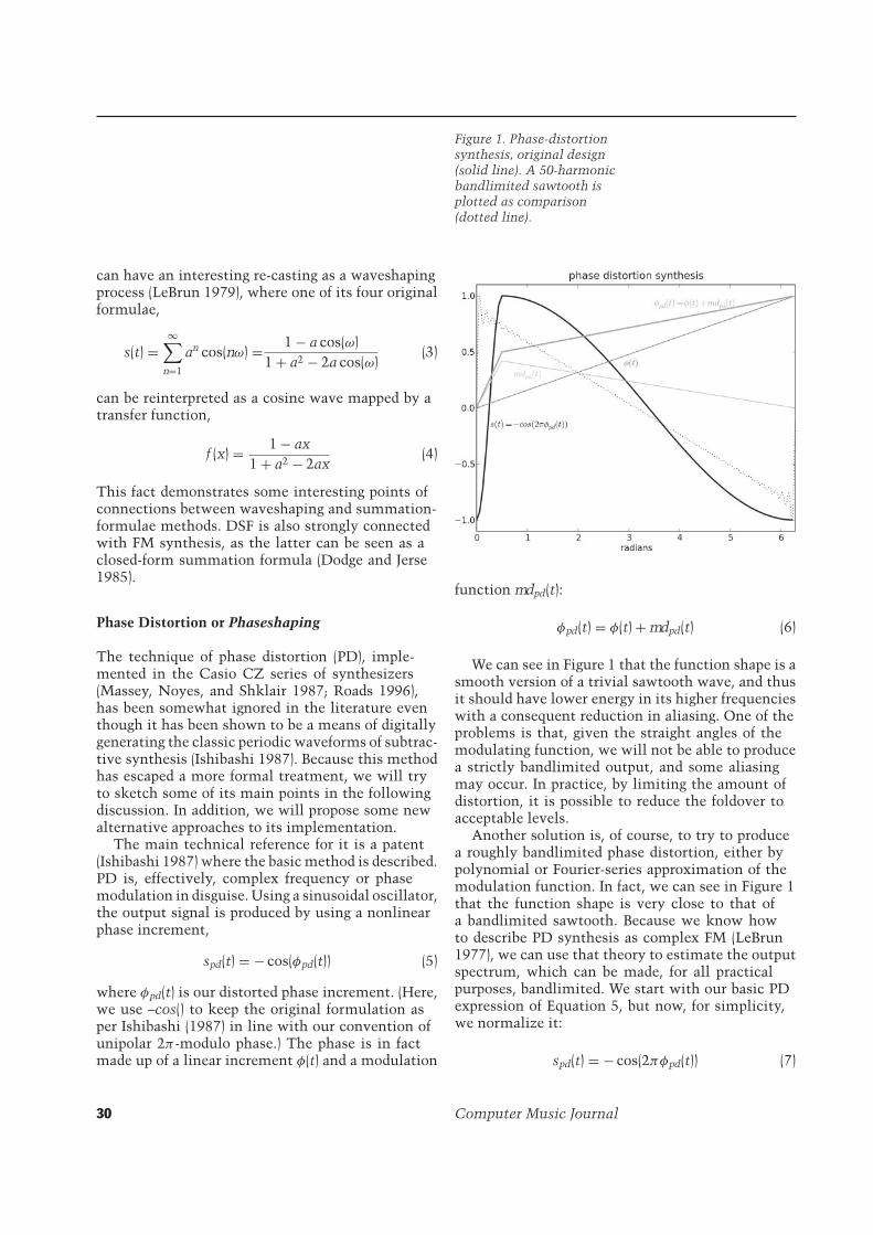
It is safe to assume that the highest componentswill be of very little amplitude, because the valueof J1(I) in those cases will be very close to 0. So,in fact, the bandwidth might be slightly less thanpredicted by the expression above. Figures 2 and3 show the result of this method in the time andfrequency domains.

In general, PD can be considered a special caseof FM synthesis in which the modulator functionfundamental frequency is an integral multiple of thecarrier frequency. For the sawtooth approximation,these are the same, whereas for a square-wavesimulation, we would want the modulator frequencyto be twice that of the carrier. In that case, fora bandlimited approach, we would model themodulator as a triangle wave.

From a complementary angle, if we understandPD to be a method of nonlinear phaseshaping, inanalogy to waveshaping, we can produce similar-sounding outputs by developing a much simpleralgorithm. One way of approximating the original“kinked” phase increment function of Figure 1 can


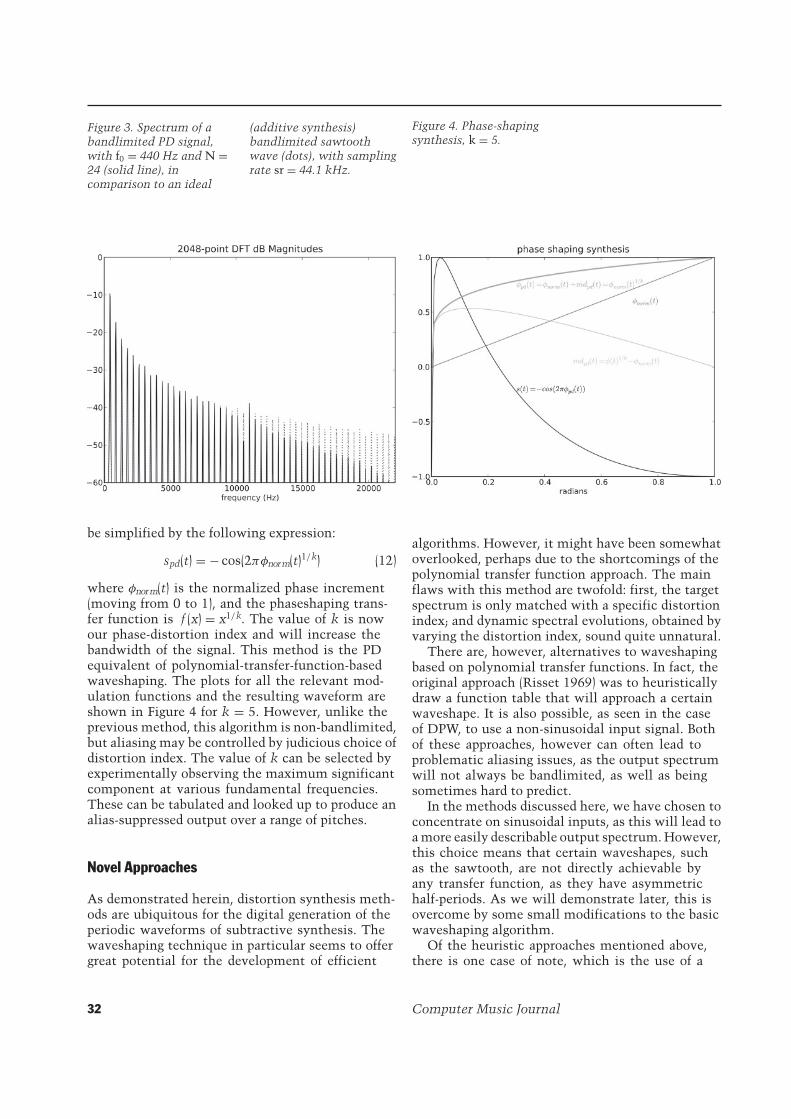
Figure 3. Spectrum of abandlimited PD signal,with f0 = 440 Hz and N =24 (solid line), incomparison to an ideal

(additive synthesis)bandlimited sawtoothwave (dots), with samplingrate sr = 44.1 kHz.

be simplified by the following expression:

spd(t) = − cos(2πφnorm(t)1/k) (12)

where φnorm(t) is the normalized phase increment(moving from 0 to 1), and the phaseshaping trans-fer function is f (x) = x1/k. The value of k is nowour phase-distortion index and will increase thebandwidth of the signal. This method is the PDequivalent of polynomial-transfer-function-basedwaveshaping. The plots for all the relevant mod-ulation functions and the resulting waveform areshown in Figure 4 for k = 5. However, unlike theprevious method, this algorithm is non-bandlimited,but aliasing may be controlled by judicious choice ofdistortion index. The value of k can be selected byexperimentally observing the maximum significantcomponent at various fundamental frequencies.These can be tabulated and looked up to produce analias-suppressed output over a range of pitches.

Novel Approaches

As demonstrated herein, distortion synthesis meth-ods are ubiquitous for the digital generation of theperiodic waveforms of subtractive synthesis. Thewaveshaping technique in particular seems to offergreat potential for the development of efficient

Figure 4. Phase-shapingsynthesis, k = 5.

algorithms. However, it might have been somewhatoverlooked, perhaps due to the shortcomings of thepolynomial transfer function approach. The mainflaws with this method are twofold: first, the targetspectrum is only matched with a specific distortionindex; and dynamic spectral evolutions, obtained byvarying the distortion index, sound quite unnatural.

There are, however, alternatives to waveshapingbased on polynomial transfer functions. In fact, theoriginal approach (Risset 1969) was to heuristicallydraw a function table that will approach a certainwaveshape. It is also possible, as seen in the caseof DPW, to use a non-sinusoidal input signal. Bothof these approaches, however can often lead toproblematic aliasing issues, as the output spectrumwill not always be bandlimited, as well as beingsometimes hard to predict.

In the methods discussed here, we have chosen toconcentrate on sinusoidal inputs, as this will lead toa more easily describable output spectrum. However,this choice means that certain waveshapes, suchas the sawtooth, are not directly achievable byany transfer function, as they have asymmetrichalf-periods. As we will demonstrate later, this isovercome by some small modifications to the basicwaveshaping algorithm.

Of the heuristic approaches mentioned above,there is one case of note, which is the use of a


hard-clipping signum function defined as

sgn(x) =

⎧⎪⎨⎪⎩

+1, x > 00, x = 0−1, x < 0

(13)

This function, when used in waveshaping, pro-duces a non-bandlimited square wave. By smoothingthe transition around the origin, it is possible toreduce the amount of aliasing that this transfer func-tion produces. The first of the methods proposed inthis section, based on hyperbolic tangent waveshap-ing, explores the implications of this principle.

In addition, there are alternative approaches fortransfer function design, based on functions withinfinite polynomial expansions (Taylor’s series),such as cos(), sin(), arccos(), arcsin(), and exp(). Theyallow for the synthesis of nearly bandlimited spectra,which is a very useful quality for VA algorithms.FM synthesis has also been demonstrated to usesuch an approach, as it can be put in terms of awaveshaping expression using sinusoidal transferfunctions (LeBrun 1979; Lazzarini, Timoney, andLysaght 2008b). However, the major problem in thiscase is that the resulting spectra will be weighted byBessel functions of the first kind. These will result inequally unnatural spectral evolutions, comparableto the results of polynomial waveshaping.

The exponential function, however, is an inter-esting case. The resulting spectrum in this caseis defined in terms of modified Bessel functionsof the first kind, which produces a more naturaltimbral evolution. The second method discussedsubsequently takes advantage of this fact to generatebandlimited pulse waveforms as the basis for classicanalog waveform synthesis.

Hyperbolic Tangent Waveshaping

The use of the hyperbolic tangent function, tanh(), inwaveshaping is quite widespread, especially in non-linear amplification modeling (Huovilainen 2005).This method has not been previously explored forthe design of VA oscillator algorithms, however. Inthis section, we present a method for generating clas-sic analog waveshapes based on this technique. The

main advantage of using sigmoids (i.e., functionsexhibiting an “s” shape), in general—and the tanh()function in particular—is the fact that their shape ap-proximates the signum shape, with a smoothed tran-sition. The hyperbolic tangent has a partial Taylor’sseries description, which can be useful for predictingthe output spectrum of waveshaping (Zucker 1965):

tanh(x) = x − x3

3+ 2x5

1.5− 17x7

315+ · · ·

=∞∑

n=1

22n(22n − 1)B2nx2n−1

(2n)!, |x| ≤ π

2(14)

where Bi represents the Bernoulli number i, definedas

B2n = (−1)n+1 2(2n)!

(2π )2n

[1 +

∞∑m=0

1m2n

](15)

If we derive this function with an input sinewave, we will obtain the following spectrum, whichis in practice bandlimited:

tanh(π

2sin(ω)

)

=∞∑

n=1

22n(22n − 1)B2n (π/2)2n−1

(2n)!sin2n−1(ω) =

=∞∑

n=1

22n(22n − 1)B2n (π/2)2n−1

(2n)!×

[2

22n−1

n−1∑k=0

(−1)n−k−1(

2n−1k

)sin([2n − 2k− 1]ω)

]=

=∞∑

n=1

n−1∑k=0

(−1)n−k−1 2B2n(22n − 1)(π/2)2n−1

n(k!)(2n − k− 1)!

× sin([2n − 2k− 1]ω) (16)

where ω = 2π ft.This will produce a signal with odd harmonics,

but with a very steep spectral rolloff (see Figure 5),which is not what we want when we are trying toproduce a digital version of an analog square-waveoscillator. However, if we consider that thehyperbolic tangent approximates a signum function


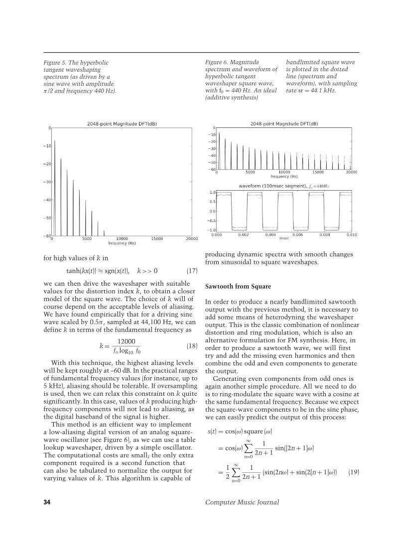
Figure 5. The hyperbolictangent waveshapingspectrum (as driven by asine wave with amplitudeπ/2 and frequency 440 Hz).

for high values of k in

tanh(kx(t)) ≈ sgn(x(t)), k >> 0 (17)

we can then drive the waveshaper with suitablevalues for the distortion index k, to obtain a closermodel of the square wave. The choice of k will ofcourse depend on the acceptable levels of aliasing.We have found empirically that for a driving sinewave scaled by 0.5π , sampled at 44,100 Hz, we candefine k in terms of the fundamental frequency as

k = 12000fo log10 f0

(18)

With this technique, the highest aliasing levelswill be kept roughly at –60 dB. In the practical rangesof fundamental frequency values (for instance, up to5 kHz), aliasing should be tolerable. If oversamplingis used, then we can relax this constraint on k quitesignificantly. In this case, values of k producing high-frequency components will not lead to aliasing, asthe digital baseband of the signal is higher.

This method is an efficient way to implementa low-aliasing digital version of an analog square-wave oscillator (see Figure 6), as we can use a tablelookup waveshaper, driven by a simple oscillator.The computational costs are small; the only extracomponent required is a second function thatcan also be tabulated to normalize the output forvarying values of k. This algorithm is capable of

Figure 6. Magnitudespectrum and waveform ofhyperbolic tangentwaveshaper square wave,with f0 = 440 Hz. An ideal(additive synthesis)

bandlimited square waveis plotted in the dottedline (spectrum andwaveform), with samplingrate sr = 44.1 kHz.

producing dynamic spectra with smooth changesfrom sinusoidal to square waveshapes.

Sawtooth from Square

In order to produce a nearly bandlimited sawtoothoutput with the previous method, it is necessary toadd some means of heterodyning the waveshaperoutput. This is the classic combination of nonlineardistortion and ring modulation, which is also analternative formulation for FM synthesis. Here, inorder to produce a sawtooth wave, we will firsttry and add the missing even harmonics and thencombine the odd and even components to generatethe output.

Generating even components from odd ones isagain another simple procedure. All we need to dois to ring-modulate the square wave with a cosine atthe same fundamental frequency. Because we expectthe square-wave components to be in the sine phase,we can easily predict the output of this process:

s(t) = cos(ω) square (ω)

= cos(ω)∞∑

n=0

12n + 1

sin([2n + 1]ω)

= 12

∞∑n=0

12n + 1

(sin(2nω) + sin(2[n + 1]ω)) (19)


Figure 7. Magnitudespectrum and waveform ofhyperbolic tangentwaveshaper sawtoothwave, with f0 = 440 Hz. Anideal (additive synthesis)

bandlimited sawtoothwave is plotted in thedotted line (spectrum andwaveform), with samplingrate sr = 44.1 kHz.

= 12

[(1 + 1

3

)cos(2ω) +

(13

+ 15

)cos(4ω) + ...

]

=∞∑

n=0

2n + 24n2 + 8n + 3

sin(2[n + 1]ω)

The resulting signal s(t) is itself made up of evenand odd harmonics of 2ω, twice the square wave’sfundamental frequency, and it is not too far from asawtooth shape. If we add together the odd and evencomponents, we will have a sawtooth-like wave atfo, defined by (excluding a normalizing factor of 0.5):

saw(t) = square (ω)(cos(ω) + 1)

=∞∑

n=0

12n + 1

sin([2n + 1]ω)

+ 2n + 24n2 + 8n + 3

sin(2[n + 2]ω) (20)

This models the sawtooth shape relatively well(see Figure 7). Remembering that in our notationthe expected amplitudes of the sawtooth’s evenharmonics are (2n + 2)−1, the approximation errorcan be calculated by

erreven harmonics(n) = 20 log10

(2n+2

4n2+8n+3

)( 1

2n+2

) (21)

Figure 8. Hyperbolictangent waveshaperoscillator flowchart.

The only significant difference is at the secondharmonic, where the error is 2.5 dB. From the fourthharmonic upward, the error is less than 0.5 dB.This is a general method that can be used with anybandlimited square-wave input. We can thereforeinsert our hyperbolic-tangent waveshaper squareinto it to produce a sawtooth. In addition, we canalso define a control m, 0 ≤ m ≤ 1, that will affectthe blend of even and odd harmonics. This, togetherwith the waveshaping modulation index, can beused to model the shape control customarily foundin analog oscillators (Moog 2002).

The complete expression for the algorithmbecomes

s(t) = A(k)(1 − m

2

)tanh

(πksin(ω)

2

)[1 + m cos(ω)]

(22)where A(k) is a scaling function used to normalizethe signal for different values of k. Smooth changesin the shape of the wave can be achieved by varyingthe value of m from 0 to 1 in Equation 22. As mapproaches 0, the expression becomes closer toEquation 17, thus producing only odd harmonics.The larger the value of m (within its correct range),the more prominent even harmonics become. Thesignal flowchart for this instrument is shown inFigure 8.


Modified FM Synthesis

Modified FM (ModFM; Timoney, Lazzarini, andLysaght 2008) is a technique derived from classicFM synthesis. The main difference between thetwo techniques is that its expansion is based onmodified Bessel functions, rather than the ordinaryBessels found in the expansion of FM equations. Therelationship between the two techniques is betterexplained first by manipulating the simple FMformulation (expressed in terms of cosines ratherthan sines):

sF M(t) = cos(ωc + kcos(ωm))

= cos(kcos(ωm)) cos(ωc) − sin(kcos(ωm)) sin(ωc)

= Jo(k) cos(ωc) +∞∑

n=1

(−1)int( n2 ) Jn(k)

× (cos(ωc − nωm) + (−1)n cos(ωc + nωm)) (23)

where Jn(k) is the Bessel function of order n, andint(n) is the integer part of the number n. Bearingin mind the expression above, ModFM is thenexpressed as

sModF M(t) = ekcos(ωm) cos(ωc)

= Io(k) cos(ωc) +∞∑

n=1

In(k) (cos(ωc − nωm)

+ cos(ωc + nωm)) (24)

with In(k) = i−nJn(ik), the modified Bessel functionof order n, which is a special case of that functionfor purely imaginary arguments (Watson 1944).

If FM synthesis can be seen as a combination ofsinusoids ring-modulated by sinusoidal-waveshapersignals, ModFM is then based on a sinusoid ring-modulated by an exponential-waveshaper signal.Other points of connection between the two ex-pressions above are discussed in Moorer (1976) andPalamin, Palamin, and Ronveaux (1988), wherevariations on a similar algorithm are explored. Themain advantage of ModFM when applied to the pro-duction of the waveforms of subtractive synthesisis that, unlike FM, ModFM exhibits a smootherand more natural-sounding spectral evolution for

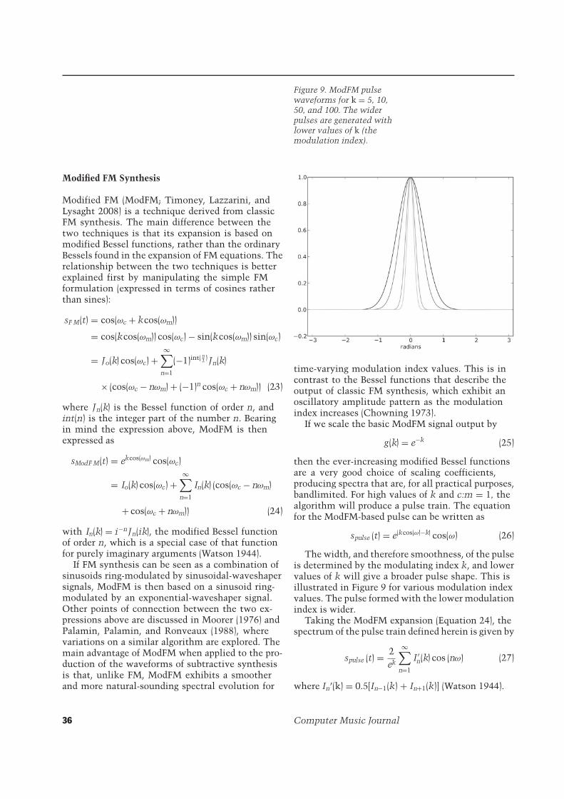
Figure 9. ModFM pulsewaveforms for k = 5, 10,50, and 100. The widerpulses are generated withlower values of k (themodulation index).

time-varying modulation index values. This is incontrast to the Bessel functions that describe theoutput of classic FM synthesis, which exhibit anoscillatory amplitude pattern as the modulationindex increases (Chowning 1973).

If we scale the basic ModFM signal output by

g(k) = e−k (25)

then the ever-increasing modified Bessel functionsare a very good choice of scaling coefficients,producing spectra that are, for all practical purposes,bandlimited. For high values of k and c:m = 1, thealgorithm will produce a pulse train. The equationfor the ModFM-based pulse can be written as

spulse (t) = e(kcos(ω)−k) cos(ω) (26)

The width, and therefore smoothness, of the pulseis determined by the modulating index k, and lowervalues of k will give a broader pulse shape. This isillustrated in Figure 9 for various modulation indexvalues. The pulse formed with the lower modulationindex is wider.

Taking the ModFM expansion (Equation 24), thespectrum of the pulse train defined herein is given by

spulse (t) = 2ek

∞∑n=1

I ′n(k) cos (nω) (27)

where In’(k) = 0.5[In−1(k) + In+1(k)] (Watson 1944).


Figure 10. Plot of thescaling functions 2e−kI′n(k)for n = 0 to 3, found in theModFM expression.

The spectrum of the modFM pulse has a low-pass characteristic. This roll-off pattern suggeststhat it should be possible to carefully chooseparameter values for the modulation index k in theequation above such that the pulse train waveformis effectively a bandlimited signal.

The rate of rolloff in the spectrum is determinedby the modulation index k and the scaled modifiedBessel functions of different orders. A plot of theamplitudes of the scaling functions in the ModFMpulse expansion (Equation 27) is shown in Figure 10.Notice that these curves are free of the characteristicwobble of classic FM Bessel functions.

Bandlimited Sawtooth Generation

If a bandlimited pulse train is available, it ispossible to generate a bandlimited sawtooth waveby integration, following the procedure given inStilson (2006, p. 214). The integration can be carriedout using a one-pole filter whose z-transform is

H (z) = 11 − z−1 (28)

An important factor in the procedure is to removethe mean of the pulse train so that the sawtooth willbe centered around a DC level of 0. For this effectin real-time implementations, we chose to use the

Figure 11. Magnitudespectrum and waveform ofModFM sawtooth wave(solid line), with f0 =440 Hz, compared to an

ideal bandlimitedsawtooth wave (dottedline), with sampling rate sr= 44.1 kHz.

linear-phase DC blocking filter given in Yates andLyons (2008) after the integration stage. A plot of theresulting signal in the time and frequency domainis shown in Figure 11. The bandlimited-sawtooth-generation system could thus be described by theblock diagram in Figure 12.

We must determine the best value for the modu-lation index k such that we achieve both our goalsof bandlimited output and sawtooth approximation.We demonstrated in the previous section that thehigher the modulation index k, the greater the mag-nitude of the higher-frequency spectral harmonics.However, from Equation 27, our output signal istheoretically not bandlimited, so high values of kcould introduce aliasing. It is clear a trade-off mustbe found between a sufficiently bright spectrumthat closely approximates a sawtooth and one free ofperceptible aliasing. By integrating Equation 27 withrespect to frequency, we will find an expression forour ModFM sawtooth wave:

ssaw(t) = 2ek (nω)

∞∑n=1

I ′n (k) sin (nω) (29)

We can now find a maximum value for themodulation index at any sawtooth frequency suchthat the harmonics that lie beyond half the samplingfrequency are less than a defined threshold. Inaddition, due to the low-pass characteristic of thesawtooth wave, we only need to know the magnitude


Figure 12. The ModFMsawtooth oscillatorflowchart.

of the first harmonic that appears above half thesampling frequency. Using a –90 dB threshold (withrespect to the fundamental frequency f0), we can findthe best values for k using the following expression:

maxk

{20 log10

I ′n+1(k)(n + 1)−1

I ′1(k)

}≤ −90dB, n =

⌊sr

2 f0

⌋

(30)

where sr is the sampling rate in Hz.Using Equation 30 to compute the maximum

value of modulation index, it was found thatits value decreases exponentially with respect tofrequency, or linearly with respect to the equivalentMIDI note number. A first-order polynomial wasfitted to the line, which then provides the expressionfor the maximum modulation index

k = e−0.1513N+15.927 (31)

where N is the MIDI note value of the desired pitchof the bandlimited sawtooth wave to be generated,defined as

N = 12 log2 ( f /440) + 69 (32)

with f in units of Hz. The modulation index is highfor low fundamentals, but smaller than unity at theother extreme of the range.

Generating Other Bandlimited Waveforms

Other waveforms can be produced following asimilar method, but using a bipolar pulse as thestarting point. This signal can easily be generated byusing a ModFM c:m ratio of 1:2:

sbipulse (t) = e(kcos(2ω)−k) cos(ω) (33)

The resulting bipolar bandlimited pulse wave isshown in Figure 13. Integrating this waveform usingthe first-order filter defined in Equation 28 thenproduces a bandlimited square wave. The resultingsquare wave is shown in Figure 14. As the methodis basically the same as for the sawtooth wave,changes to the oscillator waveshape are controlledby simple c:m ratio selection. The only limitationis that continuous smooth changes are not possible.This is because values for c:m that do not closelyapproximate ratios of small integers will result ininharmonic spectra.

In addition, if we start from a square wave,we can also produce a sawtooth wave using themethod outlined previously in Equations 19 and20. One advantage of such an algorithm is that theDC-blocking requirement is effectively removed,as the bipolar pulse in general has an insignificantDC component. In this case, the transition betweensawtooth and square can be made simpler and linear.

Finally, by further integrating the square wave, wewill also be able to produce a triangle waveform. Inthis case, we will again have to take care of removingthe signal mean, using the same DC-blocking filterof the previous section. Other ad hoc shapes can alsobe produced by the choice of various c:m ratios.


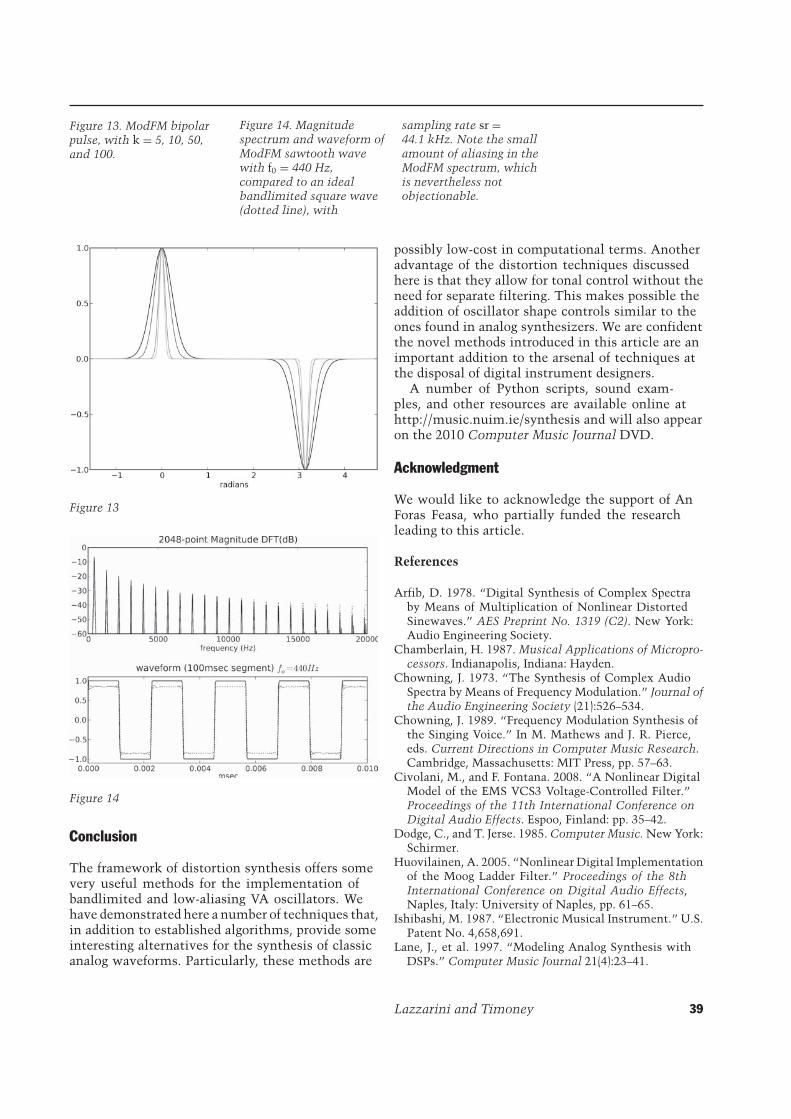
Figure 13. ModFM bipolarpulse, with k = 5, 10, 50,and 100.

Figure 13

Figure 14. Magnitudespectrum and waveform ofModFM sawtooth wavewith f0 = 440 Hz,compared to an idealbandlimited square wave(dotted line), with

sampling rate sr =44.1 kHz. Note the smallamount of aliasing in theModFM spectrum, whichis nevertheless notobjectionable.

Figure 14

Conclusion

The framework of distortion synthesis offers somevery useful methods for the implementation ofbandlimited and low-aliasing VA oscillators. Wehave demonstrated here a number of techniques that,in addition to established algorithms, provide someinteresting alternatives for the synthesis of classicanalog waveforms. Particularly, these methods are

possibly low-cost in computational terms. Anotheradvantage of the distortion techniques discussedhere is that they allow for tonal control without theneed for separate filtering. This makes possible theaddition of oscillator shape controls similar to theones found in analog synthesizers. We are confidentthe novel methods introduced in this article are animportant addition to the arsenal of techniques atthe disposal of digital instrument designers.

A number of Python scripts, sound exam-ples, and other resources are available online athttp://music.nuim.ie/synthesis and will also appearon the 2010 Computer Music Journal DVD.

Acknowledgment

We would like to acknowledge the support of AnForas Feasa, who partially funded the researchleading to this article.

References

Arfib, D. 1978. “Digital Synthesis of Complex Spectraby Means of Multiplication of Nonlinear DistortedSinewaves.” AES Preprint No. 1319 (C2). New York:Audio Engineering Society.

Chamberlain, H. 1987. Musical Applications of Micropro-cessors. Indianapolis, Indiana: Hayden.

Chowning, J. 1973. “The Synthesis of Complex AudioSpectra by Means of Frequency Modulation.” Journal ofthe Audio Engineering Society (21):526–534.

Chowning, J. 1989. “Frequency Modulation Synthesis ofthe Singing Voice.” In M. Mathews and J. R. Pierce,eds. Current Directions in Computer Music Research.Cambridge, Massachusetts: MIT Press, pp. 57–63.

Civolani, M., and F. Fontana. 2008. “A Nonlinear DigitalModel of the EMS VCS3 Voltage-Controlled Filter.”Proceedings of the 11th International Conference onDigital Audio Effects. Espoo, Finland: pp. 35–42.

Dodge, C., and T. Jerse. 1985. Computer Music. New York:Schirmer.

Huovilainen, A. 2005. “Nonlinear Digital Implementationof the Moog Ladder Filter.” Proceedings of the 8thInternational Conference on Digital Audio Effects,Naples, Italy: University of Naples, pp. 61–65.

Ishibashi, M. 1987. “Electronic Musical Instrument.” U.S.Patent No. 4,658,691.

Lane, J., et al. 1997. “Modeling Analog Synthesis withDSPs.” Computer Music Journal 21(4):23–41.


Lazzarini, V., J. Timoney, and T. Lysaght. 2007. “AdaptiveFM Synthesis.” Proceedings of the 10th Interna-tional Conference on Digital Audio Effects (DAFx07).Bordeaux: University of Bordeaux, pp. 21–26.

Lazzarini, V., J. Timoney, and T. Lysaght. 2008a. “TheGeneration of Natural-Synthetic Spectra by Means ofAdaptive Frequency Modulation.” Computer MusicJournal 32(2):12–22.

Lazzarini, V., J. Timoney, and T. Lysaght. 2008b. ”Split-Sideband Synthesis.” Proceedings of the 2008 Inter-national Computer Music Conference. San Francisco,California: International Computer Music Association,pp. 41–44.

Lazzarini, V., J. Timoney, and T. Lysaght. 2008c.“Asymmetric-Spectra Methods for Adaptive FMSynthesis.” Proceedings of the International Con-ference on Digital Audio Effects. Available online atwww.acoustics.hut.fi/dafx08/papers/dafx08 42.pdf.

Le Brun, M. 1977. “A Derivation of the Spectrum of FMwith a Complex Modulating Wave.” Computer MusicJournal 1(4):51–52.

Le Brun, M. 1979. “Digital Waveshaping Synthesis.”Journal of the Audio Engineering Society 27(4):250–266.

Massey, H., A. Noyes, and D. Shklair. 1987. A Synthesist’sGuide to Acoustic Instruments. New York: Amsco.

Moog, R. 2002. Minimoog Voyager User’s Manual.Asheville, North Carolina: Moog Music.

Moorer, J. A. 1976. “The Synthesis of Complex AudioSpectra by Means of Discrete Summation Formulas.”Journal of the Audio Engineering Society 24(9):717–727.

Moorer, J. A. 1977. “Signal Processing Aspects of Com-puter Music: A Survey.” Proceedings of the IEEE65(8):1108–1141.

Palamin, J. P., P. Palamin, and A. Ronveaux. 1988.“A Method of Generating and Controlling MusicalAsymmetric Spectra.” Journal of the Audio EngineeringSociety 36(9):671–685.

Peiper, R. 2001. “Laboratory and Computer Tests forCarson’s FM Bandwidth Rule.” IEEE 33rd SoutheasternSymposium on System Theory. Piscataway, NewJersey: Institute of Electrical and Electronics Engineers,pp. 145–150.

Puckette, M. 1995. “Formant-Based Audio SynthesisUsing Nonlinear Distortion.” Journal of the AudioEngineering Society 43(1):40–47.

Roads, C. 1996. Computer Music Tutorial. Cambridge,Massachusetts: MIT Press.

Risset, J. C. 1969. “Introductory Catalogue of Computer-Synthesized Sounds.” Reprinted in Computer Music

Currents 13 (1995). Mainz: Schott Wergo Music Media,109–254 (CD booklet).

Schottstaedt, W. 1977. “The Simulation of NaturalInstrument Tones using a Complex Modulating Wave.”Computer Music Journal 1(4):46–50.

Smith, J. O. 2008. “Physical Audio Signal Processingfor Virtual Musical Instruments and Audio Effects.”Available online at ccrma.stanford.edu/∼jos/pasp.

Stilson, T. 2006. “Efficiently-Variable Non-OversampledAlgorithms in Virtual-Analog Music Synthesis.” PhDdissertation, Department of Electrical Engineering,Stanford University. Available online at ccrma.stanford.edu/∼stilti/papers/TimStilsonPhDThesis2006.pdf.

Stilson, T., and J. Smith. 1996. “Alias-Free Digital Synthe-sis of Classic Analog Waveforms.” Proceedings of the1996 International Computer Music Conference. SanFrancisco: International Computer Music Association,pp. 332–335.

Timoney, J., V. Lazzarini, and T. Lysaght. 2008. “AModified FM Synthesis Approach to Bandlimited SignalGeneration.” Proceedings of the 11th InternationalConference on Digital Audio Effects. Espoo, Finland,pp. 27–33.

Valimaki, V. 2005. “Discrete-Time Synthesis of theSawtooth Waveform with Reduced Aliasing.” IEEESignal Processing Letters 12(3):214–217.

Valimaki, V., and A. Huovilainen. 2006. “Oscillatorand Filter Algorithms for Virtual Analog Synthesis.”Computer Music Journal 30(2):19–31.

Valimaki, V., and A. Huovilainen. 2007. “AntialiasingOscillators in Subtractive Synthesis.” IEEE SignalProcessing Magazine 24(2):116–125.

Van Der Pol, B. 1930. “Frequency Modulation.” Proceed-ings of the Institute of Radio Engineers 18(7):1194–1205.

Watson, G. N. 1944. A Treatise on the Theory of BesselFunctions, 2nd ed. Cambridge: Cambridge UniversityPress.

Winham, G., and K. Steiglitz. 1970. “Input Generatorsfor Digital Sound Synthesis.” Journal of the AcousticSociety of America 47(2):665–666.

Yates, R., and R. Lyons. 2008. “DSP Tips & Tricks [DCBlocker Algorithms].” IEEE Signal Processing Magazine25(2):132–134.

Zucker, R. 1965. “Elementary Transcendental Functions:Logarithmic, Exponential, Circular and HyperbolicFunctions.” In M. Abramowitz and I. Stegun, eds.Handbook of Mathematical Functions with Formulas,Graphs, and Mathematical Tables. New York: Dover,pp. 65–94.


Documents

VictorLazzariniandJosephTimoney NewPerspectiveson ...eprints.maynoothuniversity.ie/4104/1/VL_New_perspectives.pdf · NewPerspectiveson DistortionSynthesisfor VirtualAnalogOscillators