Pavlov and Mallama, JAAVSO Volume 43, 2015 1

1. Introduction

Analogue video cameras using CCDs with on-chip microlenses are widely used by amateurs to observe stellar occultations, meteors, planets, lunar impacts, asteroids, and comets (Mousis et al. 2014). The main advantage of video in those cases is the precise timestamps associated with each video field. Timing devices such as IOTA-VTI (VideoTimers 2011) have access to atomic time reference provided by satellites (GPS time, for example) and can timestamp each video field with a precision better than 1 millisecond (see Figure 1). The photometric data along with the precise timestamp can then be used to build light curves of the observed objects for the duration of the observation. Because of the nature of video there are no gaps in the light curves caused by dead time but there is more noise. The video observations conducted by amateurs are used in various projects driven by the professionals. An example of such a collaboration is the PHEMU09 campaign for observing

Video Technique for Observing Eclipsing Binary Stars

Hristo Pavlov9 Chad Place, St. Clair, NSW 2759, Australia; hristo_dpavlov@yahoo.com

Anthony Mallama 14012 Lancaster Lane, Bowie, MD 20715; anthony.mallama@gmail.com

Received February 9, 2015; revised March 10, 2015; accepted May 12, 2015

Abstract Video recording has been used for more than a decade to time astronomical events such as stellar occultations. We present a technique for using video to determine the time of minimum of eclipsing binary stars and we examine various aspects of using video. The free open source software packages occurec and tangra have been enhanced to offer better support for the recording and reduction of video observations of eclipsing binaries. We present our work in a style and detail that is appropriate for both video observers unfamiliar with variable stars and for variable star observers unfamiliar with video. We present the results of ten times of minima of southern eclipsing binary stars determined using the video technique.

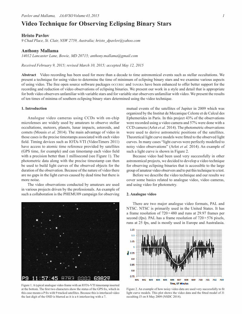
mutual events of the satellites of Jupiter in 2009 which was organized by the Institut de Mecanique Celeste et de Calcul des Ephemerides in Paris. In this project 43% of the observations were recorded using a video camera and 57% were done with a CCD camera (Arlot et al. 2014). The photometric observations were used to derive astrometric positions of the satellites. Theoretical light curve models were fitted to the observed light curves. In many cases “light curves were perfectly modelled to noisy video observations” (Arlot et al. 2014). An example of such a light curve is shown in Figure 2. Because video had been used very successfully in other astronomical projects, we decided to develop a video technique for observing eclipsing binaries that is accessible to the large group of amateur video observers and to put this technique to a test. Before we describe the video technique and our results we cover some basics related to analogue video, video cameras, and using video for photometry.

2. Analogue video

There are two major analogue video formats, PAL and NTSC. NTSC is primarily used in the United States. It has a frame resolution of 720 × 480 and runs at 29.97 frames per second (fps). PAL has a frame resolution of 720 × 576 pixels, runs at 25 fps, and is mostly used in Europe and Australasia.

Figure 1. A typical analogue video frame with an IOTA-VTI timestamp inserted at the bottom. The first two characters show the status of the GPS fix, which in this case means a P fix with 9 tracked satellites. Because this is interlaced video the last digit of the OSD is blurred as it is a 6 interleaving with a 7.

Figure 2. An example of how noisy video data are used very successfully to fit light curve models. This plot shows the video data and the fitted model of J1 occulting J3 on 8 May 2009 (NSDC 2014).

Pavlov and Mallama, JAAVSO Volume 43, 20152

According to the standard each video frame consists of two interleaving half-height video fields which are sent sequentially. Because of this the CCD chip of analogue video cameras is read differently—first the odd lines are read and sent as a video field and then the even lines are read and sent as another video field. In order to reconstruct the video frame the horizontal lines from each video field are alternated to build up the full-height image. As the analogue video standard has been developed for the images to be watched on a TV screen, a so-called Gamma correction can be applied to the produced video frames. This is an exponential per-pixel correction which will modify the image in such a way that when it is displayed by the TV screen, the brightness of the displayed objects will match closely that of the recorded objects because Gamma will reverse the non-linearity of the TV. In the old days Gamma was always applied unconditionally. In astronomy the analogue video frames will be recorded and displayed in a digital format; a Gamma of 1.00 should be applied when observations are to be used for photometry. Modern video cameras used in astronomy typically allow Gamma to be controlled and to be turned off completely by setting it to 1.00. This guarantees that the resulting system response due to off-sensor processing will not deviate from linearity. The sensor itself may still have a non-linear response, and should be tested, but modern video cameras use recently-developed CCD chips which are expected to have a largely linear response. The other important difference of analogue video is the bit depth of the pixels—8-bit, compared to the typical 16-bit depth produced by CCD cameras. While this may suggest that video offers significantly lower photometric resolution, in reality this is not exactly the case. This is because video observers adjust the linear Gain of the video camera until the stars appear bright enough but not saturated. This means that video records will usually use most or all of the 8 bits. In contrast, CCD cameras may use a lot less than the 16 bits they support, particularly with shorter exposures that do not lead to levels close to saturation. We can say that while CCD cameras will remain superior when it comes to pixel bit depths and small noise in the domain of shorter exposures, video can produce images with a dynamic range that is comparable to that of a CCD camera running in a short exposure regime.

3. Integrating video cameras

The typical video frame exposure is 40 ms for PAL and 33.37 ms for NTSC, which is insufficient for faint objects. Video cameras perform long exposures by integrating. While the exposure needs to be increased so more light is collected by the CCD chip, at the same time the camera must conform to the analogue video standard by sending video fields with the corresponding constant frame rate. Different models of video cameras may implement this slightly differently, but, generally speaking, all of them will use some sort of an internal buffer to copy the latest long exposure to and then will send this image with the required frame rate while taking another long exposure. Because there must be no dead time and all video frames are sent with the same frequency, the exposures of the video cameras, called integration rates, are a whole number of standard video

frame durations and they typically double; for example, × 2, × 4, × 8, ×16, × 32, × 64, ×128, and × 256. In PAL the × 4 integration rate will correspond to a 160 ms exposure. There are two issues to be dealt with as a result of the operation of integrating video cameras. The first issue is that the integrated image is sent after it has been taken and the timestamp associated with it, inserted during the transmission of the individual video fields, will be off by a constant amount that depends on the camera model and the integration rate which was used. Also, all individual video fields will be time stamped even though they are different fields representing the same long exposure. All this complicates the determination of the time of the exposure. This problem is solved, however, by experimentally determining the so-called Instrumental Delay of each video camera model and each supported exposure and then applying a correction to derive the exact time of the mid-exposure. Most popular video cameras used for astronomy have been tested and their Instrumental Delays are well known (Dangl 2008). This allows photometric data reduced from video to be timed with a precision of milliseconds from UTC. The second issue to be addressed is that the video produced by integrating cameras will still run at a constant high frame rate even though the exposure is longer. If a standard video recording software is used, a two-hour constant monitoring of a star could produce a file size of 100 to 200 gigabytes. This could create a storage problem as well as data reduction difficulty due to the file size. Also, there is a need to deal with the many repeated video frames of the same image during the data reduction. In order to address those issues we use the custom-built video recording software, occurec, which is described next.

4. Recording software

occurec (Pavlov 2014) is open source software for windows that allows multiple video frames to be stacked on the fly so the effective frame rate of the video is reduced by saving only one video frame from a physical exposure or combining multiple exposures into one single video frame (Pavlov 2014). This can significantly decrease the recorded file size, making it easier to record video for hours, and it also improves the signal-to-noise ratio (SNR) as a result of the stacking. A new Astro Analogue Video (AAV) open source and lossless file format is used to save the video. AAV is an extension of the Astronomical Digital Video (ADV) file format (Barry et al. 2013) customized for analogue video. Because multiple 8-bit video frames are stacked and saved as one, the resulting AAV video bit depth will be more than 8 bits—up to 12 bits with the typical number of frames being stacked. In our observations of eclipsing binary stars we use occurec as the video recording software. Apart from the convenience of scheduled recording and telescope and video camera control, it offers better SNR and bit depth with a much smaller file size. The stars that we observed were in the range from magnitude 9 to 12 . This was bright for the 14-inch telescope and the very sensitive WAT-910BD video camera so no video integration was required. Because of this occurec was run in a stacking mode

Pavlov and Mallama, JAAVSO Volume 43, 2015 3

in which it combines multiple exposures into a single video frame. A stacking of × 8, ×16, and × 32 was used with the PAL camera, which produced effective exposures of 320 ms, 640 ms, and 1,280 ms.

5. Reduction software

The data reduction has two distinct parts. The first is reducing photometric data from the video and producing a light curve, and the second is analyzing the light curve data to derive a time of minimum (TOM) for the observed star. To reduce photometric data from the video we use the tangra software package (Pavlov 2014). It works with AAV files and has been used previously for video data reduction by a number of researchers (Kitting et al. 2012; Sposetti et al. 2012; Lena et al. 2014). tangra offers a range of measurement options including aperture photometry, PSF photometry, and various ways to measure the background. For analogue video where the smaller bit depth may result in a lot fewer unique light levels for a pixel, we recommend using Aperture Photometry with Average Background. tangra offers an open add-in based integration which allowed us to build an add-in module that implements the standard analysis algorithm of Kwee and van Woerden (1956) to derive a time of minimum and an estimate of its uncertainty from the light curve data (Mallama and Pavlov 2015). The add-in automatically applies the correction for the Heliocentric Julian Day (HJD) from the determined JD of the minimum and reports the TOM in HJD. tangra and occurec have been traditionally used for occultations and to time shorter events with higher precision. During the development and testing of the video technique for observing eclipsing binaries, a number of improvements were made in both software packages to ensure the smooth operation and ease of processing of observations of those stars.

6. Observational guidelines

In order to determine the TOM from a single video observation the record has to be long enough to contain a large number of data points during both the descending and ascending branches of the light curve. If the star exhibits a total eclipse with a flat bottom in the light curve the record has to be even longer. Stars with periods less than one day are typically better suited for video observations as they usually show faster change in brightness. For them, a recording of one to two hours on each side of the minimum/flat bottom is sufficiently long. During such a long observation the light from the target and comparison stars will pass through varying air masses as their altitude changes. As a result, if there is a large difference in the color of the target and comparison stars there will be a systematic error during the normalization which could affect the determination of the TOM. While we recommend the use of a photometric filter, this is not strictly required. “Taking unfiltered images is usually OK when the target is more than 30 degrees above the horizon or when the variable and comparison stars are the same color. Trouble could happen with unfiltered images of stars close to the horizon.” (Samolyk 2015).

7. Observational results

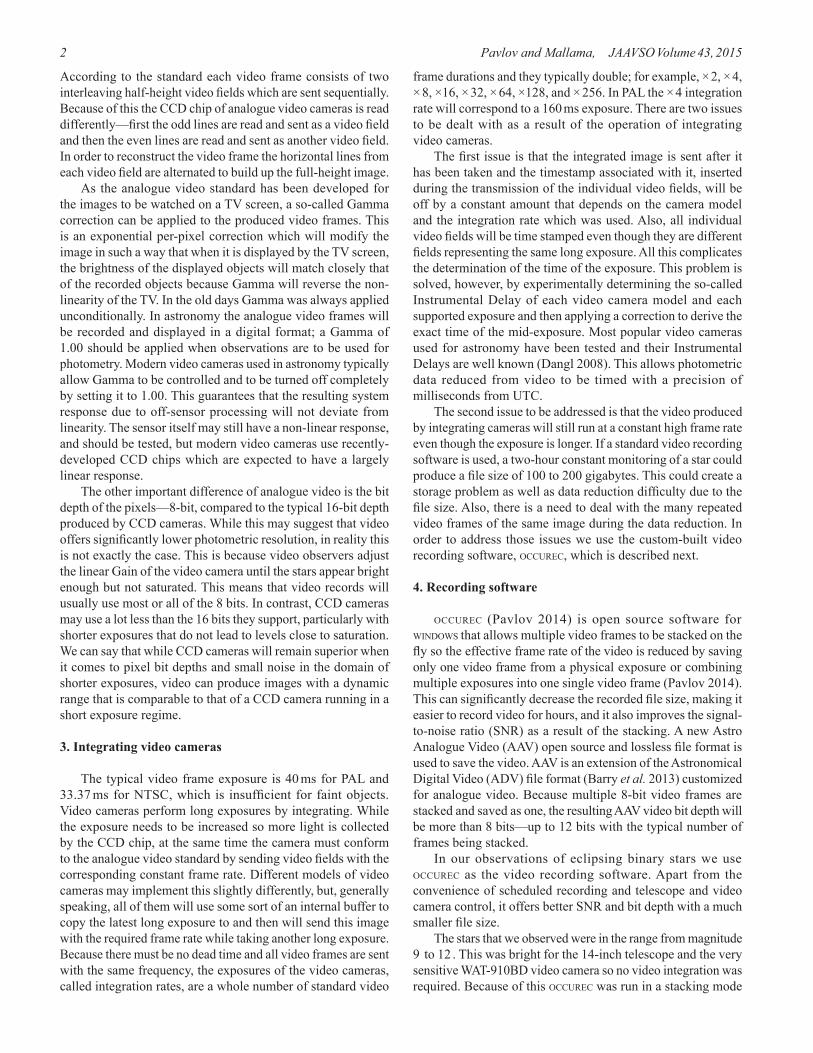
Video observations using the described technique were done at Tangra Observatory (IAU Code E24) by one of the authors (HP; AAVSO code PHRA) using a 14-inch LX-200 ACF and WAT-910BD TACOS video system (Gault 2014). Most observations were done with a Sloan r' filter. Ten times of minima of eight southern stars were determined and are given in Table 1. We used observations and O–C data from (Nelson 2014) and (Paschke 2015) to verify our measurements and to refine the ephemeris of one of the stars we observed. CG Pup is a semi-detached Algol-type binary that ranges from photographic magnitude 10.2 to 13.0 according to the AAVSO International Variable Star Index (VSX; Watson et al. 2014). The variability was discovered by Hoffmeister (1943) and TOMs prior to the present study were derived from photographic observations. One of the two video light curves for CG Pup is shown in Figure 3. The O–C values for the ephemeris in the General Catalogue of Variable Stars (GCVS; Kholopov et al. 1985) for the video TOMs were 0.38185 and 0.38171 day, which are more than one-third of the orbital period. The difference between the two O–C values, 0.00016 day, matches well with the reported TOM uncertainty of 0.0001.

Table 1. Times of minima of southern stars determined using the video technique in the period December 2014 to February 2015, in addition to one value derived from ASAS photometry.

Star Type Time of Minima Uncertainty Comment (HJD)

WZ Ant I 2457061.9718 0.0006 r' GW Car I 2457037.1644 0.0004 r' V576 Cen I 2457057.1027 0.0003 r' FT Lup I 2457061.1252 0.0002 r' ER Ori I 2457011.9964 0.0003 clear ER Ori I 2457025.9693 0.0002 r' CG Pup I 2457036.9680 0.0001 r' CG Pup I 2457039.0670 0.0001 r' CG Pup I 2453286.8054 ASAS data UX Ret I 2457009.9654 0.0003 clear DS Vel I 2457029.9710 0.0003 r'

Figure 3. A tangra light curve of the minimum of CG Pup that contains more than 12,000 data points. The observation is done with a SLOAN r' filter and the light curve is very symmetrical. The curved band represents the variable and the horizontal band the comparison star.

Pavlov and Mallama, JAAVSO Volume 43, 20154

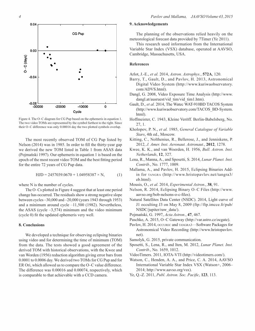
The most recently observed TOM of CG Pup listed by Nelson (2014) was in 1985. In order to fill the thirty-year gap we derived the new TOM listed in Table 1 from ASAS data (Pojmański 1997). Our ephemeris in equation 1 is based on the epoch of the most recent video TOM and the best fitting period for the entire 72 years of CG Pup data.

HJD = 2457039.0670 + 1.04958387 × N, (1)

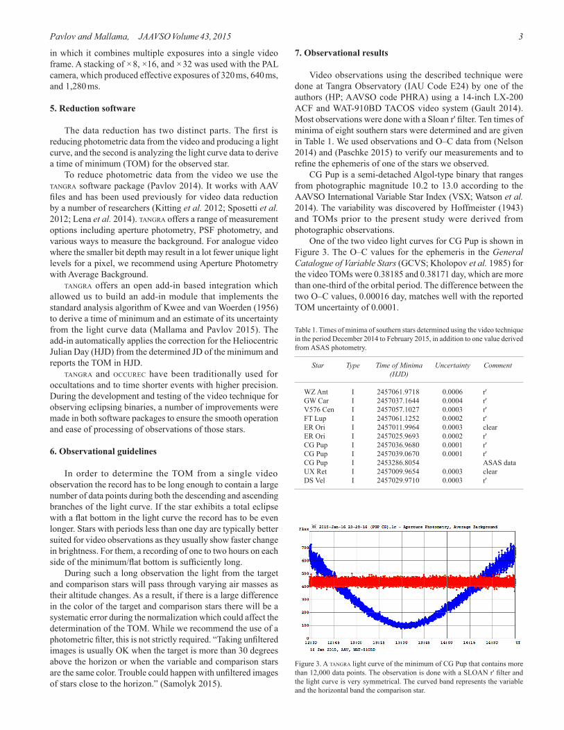
where N is the number of cycles. The O–Cs plotted in Figure 4 suggest that at least one period change has occurred. The residuals show a strong negative slope between cycles –30,000 and –20,000 (years 1943 through 1953) and a minimum around cycle –11,500 (1982). Nevertheless, the ASAS (cycle –3,574) minimum and the video minimum (cycle 0) fit the updated ephemeris very well.

8. Conclusions

We developed a technique for observing eclipsing binaries using video and for determining the time of minimum (TOM) from the data. The tests showed a good agreement of the derived TOM with historical observations, with the Kwee and van Worden (1956) reduction algorithm giving error bars from 0.0001 to 0.0006 day. We derived two TOMs for CG Pup and for ER Ori, which allowed us to compare the O–C value difference. The difference was 0.00016 and 0.00074, respectively, which is comparable to that achievable with a CCD camera.

Figure 4. The O–C diagram for CG Pup based on the ephemeris in equation 1. The two video TOMs are represented by the symbol furthest to the right. Since their O–C difference was only 0.00016 day the two plotted symbols overlap.

9. Acknowledgements

The planning of the observations relied heavily on the meteorological forecast data provided by 7Timer (Ye 2011). This research used information from the International Variable Star Index (VSX) database, operated at AAVSO, Cambridge, Massachusetts, USA.

References

Arlot, J.-E., et al. 2014, Astron. Astrophys., 572A, 120.Barry, T., Gault, D., and Pavlov, H. 2013, Astronomical

Digital Video System (http://www.kuriwaobservatory.com/ADVS.html).

Dangl, G. 2008, Video Exposure Time Analysis (http://www.dangl.at/ausruest/vid_tim/vid_tim1.htm).

Gault, D., et al. 2014, The Watec WAT-910BD TACOS System (http://www.kuriwaobservatory.com/TACOS_BD-System.html).

Hoffmeister, C. 1943, Kleine Veröff. Berlin-Babelsberg, No. 27, 1.

Kholopov, P. N., et al. 1985, General Catalogue of Variable Stars, 4th ed., Moscow.

Kitting, C., Nolthenius, R., Bellerose, J., and Jenniskens, P. 2012, J. Amer. Inst. Aeronaut. Astronaut., 2012, 1278.

Kwee, K. K., and van Woerden, H. 1956, Bull. Astron. Inst. Netherlands, 12, 327.

Lena, R., Manna, A., and Sposetti, S. 2014, Lunar Planet. Inst. Contrib., No. 1777, 1009.

Mallama, A., and Pavlov, H. 2015, Eclipsing Binaries Add-in for tangra (http://www.hristopavlov.net/tangra3/eb.html).

Mousis, O., et al. 2014, Experimental Astron., 38, 91.Nelson, R. 2014, Eclipsing Binary O–C Files (http://www.

aavso.org/bob-nelsons-o-c-files).Natural Satellites Data Center (NSDC). 2014, Light curve of

J1 occulting J3 on May 8, 2009 (ftp://ftp.imcce.fr/pub/NSDC/jupiter/raw_data/).

Pojmański, G. 1997, Acta Astron., 47, 467.Paschke, A. 2015, O–C Gateway (http://var.astro.cz/ocgate).Pavlov, H. 2014, occurec and tangra3—Software Packages for

Astronomical Video Recording (http://www.hristopavlov.net).

Samolyk, G. 2015, private communication.Sposetti, S., Lena, R., and Iten, M. 2012, Lunar Planet. Inst.

Contrib., No. 1659, 1012. VideoTimers. 2011, IOTA-VTI (http://videotimers.com/).Watson, C., Henden, A. A., and Price, C. A. 2014, AAVSO

International Variable Star Index VSX (Watson+, 2006–2014; http://www.aavso.org/vsx).

Ye, Q.-Z. 2011, Publ. Astron. Soc. Pacific, 123, 113.