· Web viewExplicit Modelling of Large Deflection Behaviour of Restrained Reinforced Concrete Beams in Fire Sherwan Albrifkani and Yong C Wang School of Mechanical, Aerospace and Civil

Explicit Modelling of Large Deflection Behaviour of Restrained Reinforced

Concrete Beams in FireSherwan Albrifkani and Yong C Wang

School of Mechanical, Aerospace and Civil Engineering, University of Manchester, UK

Abstract

This paper presents a dynamic explicit finite element (FE) simulation method to predict the highly

nonlinear response of axially and rotationally restrained reinforced concrete (RC) beams at

ambient temperature and in fire condition. Catenary action, developed during the large deflection

behaviour of RC beams, is an important mechanism of resisting progressive collapse. This paper

explains the numerical simulation challenges, including temporary instabilities, local failure of

materials, non-convergence and long simulation time, and proposes methods to resolve these

challenges. The effectiveness of the proposed simulation model is checked by comparison of the

simulation results against relevant test results of restrained RC beams at ambient temperature and

in fire. It has been found that using the explicit simulation method can follow the whole range

behaviour of restrained RC beams until complete structural failure. Either load factoring or mass

scaling may be used to speed up the simulation process. Damping can be applied to minimise

significant dynamic effects following beam bending failure. This paper will give guidance on how

to select the appropriate load factoring, mass scaling and damping values.

Keywords: restrained RC beam; explicit modelling; fire resistance; catenary action; load factoring; mass scaling; damping; concrete

1

1. Introduction

The prescriptive-based approach to fire resistance design of reinforced concrete (RC) structures

involves specifying the minimum concrete cover and the minimum size of member cross section

depending on the load ratio, in codes such as EN 1992-1-2[1], according to the required standard

fire resistance rating. This is being progressively replaced by the performance-based approach in

which the provisions for fire resistance are according to the performance requirements.

In performance-based evaluation of the fire resistance of structures, it is necessary to consider the

interactions between different structural members. Furthermore, large deflections are involved in

structural behaviour at the high temperatures experienced in fires. At large deflections, the

structural members can develop alternative load carrying mechanisms that would not normally be

considered in small deflection analysis. For axially restrained beams, the alternative load carrying

mechanism of catenary action can develop after the conventional flexural bending mechanism.

The development of catenary action can significantly enhance the beam survival time compared to

the fire resistance estimated based on bending resistance. Whilst there have been extensive

research studies on the behaviour of axially restrained steel beams in fire, for RC beams in fire [2-

22], the effect of axial restraint is rarely considered and even when axial restraint is present [2-4,

8, 11], the research did not address the development of catenary action at very large beam

deflections.

Using catenary action as an alternative load-carrying mechanism for beams is the basis of

mitigating progressive collapse under the column removal scenario at ambient temperature and

this mechanism has been investigated in recent years [23-33]. While the same philosophy is

applicable to the fire situation, there has been little research to assess the feasibility. In order to

exploit the potential of using catenary action as a means of controlling progressive collapse in RC

structures in fire, it is necessary to be able to reliably quantify this behaviour. This is the aim of

this research.

Since conducting physical fire tests on axially restrained RC beams to observe the development of

catenary action is expensive and technically demanding, development of a robust numerical

simulation model is needed and this is the specific objective of this paper.

Many numerical models have been developed to predict the structural behaviour of RC beams at

elevated temperatures. Most of these models were proposed for unrestrained beams [5, 6, 9, 13,

16-22]. The few developed models that can be applicable to restrained RC beams in fire [3, 8, 11,

12] were specifically intended to assess the behaviour of members at small deflections under the

2

combined effects of flexural bending and axial compressive forces generated by the restraint to

thermal expansion.

Faithful numerical simulation of the large deflection structural behaviour of axially restrained RC

beams presents serious challenges due to the material failures that can occur, including concrete

cracking, crushing and reinforcement fracture (which may cause temporary loss of equilibrium of

the structure and dynamic behaviour), and very severe geometrical nonlinearities. Coupled with

changing temperatures, it is not feasible to numerically model the structure using conventional

static techniques based on the implicit approach.

This paper explores the explicit modelling approach. Although the explicit approach has been

adopted by a number of researchers [30, 34-38], its applicability to elevated temperature

modelling of restrained RC beams has not been assessed. When using the explicit time integration

algorithm, the time increment has to be very small. This makes it problematic when applying this

modelling approach to fire conditions because fire exposure has long durations. Therefore, an

important task in implementing the explicit simulation approach is to resolve this challenge.

Two techniques may be considered, either separately or together, to achieve a computationally

economical solution without compromising accuracy of the simulation. These are (a) artificially

increasing the loading speed (load factoring) and (b) artificially increasing the mass of the

structure to increase the stable time step (mass scaling).

This paper will present details of the above mentioned two approaches and provide guidance on

their implementations for 3D restrained RC beams at ambient and elevated temperatures using the

ABAQUS/Explicit solver. To validate the developed explicit modelling approach, the simulation

results will be compared against relevant test results, including the ambient temperature tests on

axially restrained RC beams by Yu and Tan [28, 32], and the fire tests on axially restrained RC

beams by Dwaikat and Kodur [2]. Unfortunately, the fire tests by Dwaikat and Kodur [2] were

terminated before the onset of catenary action. Nevertheless, these tests represent the most

relevant cases to check accuracy of the proposed simulation model of this paper.

2. Development of the explicit modelling methodology

The ambient temperature tests of Yu and Tan [28, 32] on axially restrained RC beams will be used

to explain the development of the explicit modelling approach. These tests were selected owing to

their comprehensive reporting of the test arrangement and results.

3

2.1 Brief introduction to the tests by Yu and Tan [28, 32]

Fig. 1 shows the sub-assemblage test and the frame test arrangements. The three sub-assemblage

test specimens, denoted as S4, S5 and S7, comprised of two enlarged column stubs at the ends,

two single-bay beams and one middle joint. The experiments examined the effects of varying

reinforcement ratio and beam span-to-depth ratio. In the two frame specimens, detonated as F2

and F4, the column stubs were replaced by side columns and beam extensions. Each specimen was

designed with a special technique of reinforcement detailing, aimed at enhancing the ultimate load

carrying capacity in catenary action. All specimens were loaded by applying a displacement-

controlled pushdown force at a rate of 0.1mm/s at the top of the unsupported middle joint until

failure. In the frame tests, one of the side columns was subjected to an axial stress of 0.6f′c and the

other to 0.4f′c prior to load application on the middle joint and these column loads were kept

constant during the test. Table 1 lists the main specimen details and Table 2 gives the mechanical

properties of the steel reinforcing bars. The compressive cylinder strength of concrete (f′c) for

specimens S4, S5 and S7 was 38.2 MPa, and for specimens F2 and F4 was 29.69 MPa.

2.2 Boundary conditions and load application

Much attention was paid to the simulation of the boundary conditions of the beam-column sub-

assemblages and frames. This is because there were several interactions at the supports, as

illustrated in Fig 2, and the accuracy of FE simulation results critically depend on accurate

specification of these interactions. In the laboratory tests, one end of the specimen was restrained

by an A-Frame and the other end by a reaction wall through two horizontal pin-pin connections. In

the simulation model, in order to avoid any local stress concentration, the same assembly of steel

plates and steel rods as in the tests was created in the simulation model to anchor the beams to the

connections by using the ABAQUS “Tie constraint”. “Tie restraint” was also used to connect the

top and bottom column end plates to the concrete columns. In order to simulate the pin boundary

condition as in the actual tests and to make sure that each plate rotated around the pin during the

loading process, all the plates were modelled as rigid bodies using “Rigid body constraint” in

ABAQUS.

Yu [39] provided the linear elastic stiffness of the horizontal restraints, shown in Fig. 2, and the

gaps between the restraints and the specimens. These stiffness values and the gaps were used in

the authors’ ABAQUS model when using the “Axial connector elements”. The axial loads in the

side columns of the frame models were firstly applied in one step up to the same level as in the

tests before application of the monotonically increasing load at the top of the middle joint until

failure. To save computation time, only half of the sub-assemblage test specimen was modelled

4

based on geometrical and loading symmetry. For the frame tests, the whole frame specimen was

modelled because the two side columns had different applied loads.

2.3 Material constitutive models

2.3.1. Concrete

The concrete damaged plasticity CDP model in ABAQUS was used to define the inelastic

behaviour of concrete. Damage of concrete is associated with the two main failure mechanisms,

namely tensile cracking and compressive crushing, and evaluation of the yield surface is

controlled by the equivalent plastic strains in tension and compression, respectively [40]. Table 3

lists the default ABAQUS values of the five parameters used to define the damaged plasticity

model. Fig. 3 shows the uniaxial compressive stress-strain relationship according to CEB-FIP

mode code [41] up to the peak compressive stress. The softening branch was approximately

modelled by a straight line to a stress of 0.2 fcm and the rate of strength decline was controlled by

varying the limit of maximum concrete strain n ε c1 corresponding to 0.2 fcm. Values of n between 3

and 4 were chosen in this study because they gave consistent numerical results.

Many methods may be used to model cracked concrete. When the RC beam deflections are small,

satisfactory modelling results can be obtained by using any shape as long as the area underneath

the tension softening curve is kept constant based on the tensile fracture energy Gf value and the

crack band width. Furthermore, the influences associated with slippage and bond between the

reinforcement and the concrete can be macroscopically represented by introducing tension

stiffening effects in the cracked concrete model. However, for problems involving large

deflections and severe tension cracks as in the current study, careful consideration should be made

when modelling tension softening behaviour in order to minimise numerical simulation problems

associated with strain localisation, stability loss and spurious sensitivity of modelling results to

mesh size. In addition, to allow the ABAQUS option of embedding reinforcing bars in concrete, a

more realistic tension stiffening curve is necessary. This curve should implicitly consider the

interactions between reinforcement and concrete because explicit modelling of the reinforcement-

concrete bond is time consuming. In general, according to Okamura et al [42], a power form of

tensile stress-strain curve, as and shown in Fig. 4, can be used. In Fig. 4, ε cr is the cracking strain;

c is a coefficient that controls the rate at which the tension stress σ t decreases with increasing

strain ε t after cracking. In general, the main factors that influence the magnitude of coefficient c

are tensile concrete fracture energy, element mesh size and reinforcement ratio [43, 44]. The

influence of fracture energy, which depends on element mesh size, is important when dealing with

propagation of cracks in plain concrete or concrete with very little reinforcement, in which the

5

tensile strength of concrete quickly drops to zero. However, the influences of element size become

small and are usually ignored in reinforced concrete members because the concrete between

cracks can still carry tension stresses. Therefore, in this research, the mesh size effect was not

considered and a value of c=0.4 was adopted as recommended for deformed bars [42].

2.3.2 Steel reinforcement

The uniaxial stress-strain curve of the longitudinal steel reinforcement bars (ϕ 10 and ϕ 13) is

shown in Fig. 5 according to the experimental data Table 2. An elastic perfectly plastic model was

assumed for the transverse steel bars (ϕ 6). The classical metal plasticity model available in

ABAQUS was used to model steel materials.

2.4 Introduction to dynamic explicit modelling

The explicit solution procedure is simple to implement because no global tangent stiffness and

mass matrices need to be assembled and inverted and the internal forces are determined on the

element level. However, the explicit solver is only conditionally stable and the time increment has

to be very small so that the acceleration throughout an increment can be assumed to be constant.

The maximum time increment that may be used is denoted as the stability limit. It is initially

defined as the time required by a dilatational wave across the smallest elements in the mesh, and is

estimated [40] as:

∆ t ≤ min(Le√ ρλ̂+2 μ̂ ) (1)

where Le is the element characteristic length, ρ is the mass density of the material. λ̂ and μ̂ are

Lame’s constants defined in terms of the material modulus of elasticity E and Poisson’s ratio υ as:

λ̂= Eυ(1+ν ) (1−2 ν ) (2)μ̂=

E2(1+ν)

(3)

As the analysis proceeds, the stable time increment may be defined in terms of the highest

frequency of the entire model ωmax, satisfying the following condition:

∆ t ≤2

ωmax(√1+ξmax

2−ξmax) (4)

where ξmax is the damping ratio associated with ωmax.

Two techniques may be used to control the time increment in ABAQUS/Explicit: fixed time

increment and full automatic time increment. In the former technique, a constant time increment

size smaller than the stability limit may be used. In the latter technique, the integration scheme

uses the stable time increment as the time interval to establish the numerical solution. In this

6

research, the full automatic time increment strategy is employed because it can efficiently control

the solution procedure through updating the stability limit. This is important for problems that

experience very large deformations and high material nonlinearity that cause continual changes in

the highest system frequency, thereby changing the stability limit.

2.5 Reducing computational cost

The explicit solver is intended for high speed transient events in which the inertial effects play a

significant role in the solution. For simulating the response of RC structures under fire exposure,

because the fire duration is long, the explicit simulation becomes computationally very expensive.

This is also problematic for simulating static response of structures under monotonic loading at

ambient temperature until failure occurs and for applying the targeted constant vertical load before

thermal loading starts. Therefore, an efficient simulation strategy is necessary to drastically reduce

the cost of computation but still ensure the solution is quasi-static. This may be done by either

artificially increasing the loading/temperature increase rate (load factoring technique), or

increasing the material density (mass scaling). In the load factoring approach, loads, boundary

conditions and nodal temperatures imported from a heat transfer analysis can be applied over a

shorter period of time compared to the actual event time. The mass scaling option allows for the

use of the same actual event time through increasing the density of the material so that the

dilatational wave speed within the elements is reduced, leading to increased stable time step size

and so reducing the number of increments to complete the solution. In both approaches, it is most

important to determine how much a simulation can be accelerated before the inertial forces

dominate the solution. The inertia forces should be kept very small to the extent they can be

ignored to ensure that the solution is quasi-static.

To determine the appropriate quantities to be used, the simulation results will be compared against

the test results of Yu and Tan [28, 32].

In this paper, the correlation between loading duration (LD) and the lowest natural period (T n) of

the finite element model is taken as the basis for estimating the optimal loading rate. It is assumed

that the same ratio of the applied loading time to the period of the lowest natural mode for the

successful simulation of one structure can be similarly used for other structures. This paper will

establish the minimum time ratio that can be used. Determining this minimum ratio will also

involve minimising the kinetic energy of the structure.

2.5.1 Load factoring

To illustrate this procedure, the beam-column sub-assemblage test S4 is used. Fig. 6 compares the

applied load-middle joint displacement (MJD) and beam axial force-MJD relationships between

the test data and simulations, and displays the ratio of the kinetic energy to the internal energy

7

using loading durations (LD) of 2.25, 3.5 and 5s. Displacement controlled loading method was

used and the total applied displacement during the whole LD was 700mm.The selected LD values

correspond to loading rates of 3110, 2000 and 1400 times the test rates respectively as the test

specimen was loaded at a speed of 0.1mm/s. The vertical load and the horizontal axial force in the

simulation results are summation of the reaction forces at supports. It can be seen that numerical

results converge to identical peak loads and are in a close agreement with the test results. After

fracture of the bottom reinforcement bars, the results from LD = 2.25s exhibited vibration due to

dynamic effects before they disappeared due to increased stiffness. To obtain smooth results and, a

minimum loading time of 3.5s is acceptable.

The simulations in the above example were displacement controlled as adopted in the

experimental tests. Displacement control is suitable if there is a single point loading. In most

cases, load control based simulation is necessary. In a load-controlled system, if static equilibrium

cannot be sustained, the structure may physically undergo dynamic behaviour before returning to

static stability. Therefore, it is important that simulation of the subsequent static behaviour is not

affected by the temporary dynamic behaviour. Applying some artificial damping is often adopted

to minimise undesirable dynamic effects.

Fig. 7 compares the test and load-controlled simulation results and displays the ratio of the kinetic

energy to the internal energy using LD values of 3.5, 4.5 and 6s for the same sub-assemblage test

(S4) as. The total linear applied load was 110kN and the damping ratio was 35%. Although the

same maximum load carrying capacity at the same MJD was obtained as for longer loading

durations when the loading duration was 3s, numerical oscillation during the catenary action stage

continued. Therefore, a minimum loading duration of 4.5s would be more appropriate for load-

controlled simulation.

It is assumed that successful explicit simulations of different structures have similar minimum

LD/Tn ratios, i.e.:

LD1

Tn , 1=

LD2

T n ,2

(5)

The subscripts 1 and 2 denote two different structures. In the above examples, the lowest natural

frequency ωmin1 of the model was 89.5 rad/s, giving the corresponding T n ,1 of 0.070s. The value of

ωmin can be determined from a frequency analysis via “Static, linear perturbation” procedure in

ABAQUS. Based on this example, because the minimum LD for the displacement controlled

simulation was 3.5s and that for the load controlled simulation was 4.5s, they give minimum LD/

T n of 50for displacement controlled simulation and 64 for load-controlled simulation. To

demonstrate general applicability, these values will be used when comparing the simulation results

8

with the test results for the other structures tested by Yu and Tan [28, 32] in the validation section

of this paper.

2.5.2 Material damping

The temporary instability accompanying load-controlled simulation may lead to significant

increase in kinetic energy of the system. ABAQUS/Explicit introduces a small amount of damping

in the form of bulk viscosity. This damping helps to avoid numerical issues such as element

collapse in simulating extremely high-speed dynamic problems [40]. Generally, predicting the

exact value of structural damping ratio is difficult. In the present research, Rayleigh damping in

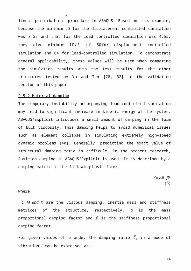
ABAQUS/Explicit is used. It is described by a damping matrix in the following basic form:

C=αM+ βK (6)

where

C, M and K are the viscous damping, inertia mass and stiffness matrices of the structure,

respectively. α is the mass proportional damping factor and β is the stiffness proportional

damping factor.

For given values of α andβ, the damping ratio ξ i in a mode of vibration i can be expressed as:

ξ i=α

2 ωi+

β ωi

2 (7)

where ωi is the natural frequency of mode i. The stiffness proportional damping factor β

dramatically reduces the stable time increment and this would influence the computational time

[40]. Thus, it is more preferable to use α to damp out undesirable modes of the structures.

Therefore, in this study, it is assumed that β=0. Eq. (7) can now be written as:

α=2ωiξ i (8)

To select an appropriate range of damping ratio, a series of models were run with different values

of ξ , introduced in the material model of both concrete and steel reinforcement. Fig. 8 compares

the vertical reaction force versus MJD of sub-assemblage test S4 for α values of 0, 27, 45, 63 and

98, which introduce 0, 15%, 25%, 35% and 55% of the structural damping ratio ξ in the lowest

mode based on ωmin =89.5 rad/s, respectively. It can be seen that the simulation model with no

damping was not able to limit numerical oscillations before final failure of the sub-assemblage is

reached. A model with low damping ratio (ξ=15%) regained stability in catenary action at larger

MJD. For models with high damping ratios (ξ ¿55%), although the simulation models were

stable, the high artificial damping dominated the structural response and prevented the structure

9

from further deformation (Fig. 8c). This result is spurious and indicates that such high level of

artificial damping is not desirable.

The above message is reinforced when the reaction force of the structure is compared between the

simulation and test results (Fig. 8d). For high damping ratios (ξ ¿55%), the simulation reaction

forces are lower than the test results. Therefore, it is recommended using damping ratio ξ in the

range between 25 %≤ ξ ≤ 35 %.

The acceptable damping factor (α ) is structure specific. However, on the assumption that

successful explicit dynamic simulations (numerical stability and minor influence of damping on

structural response) have similar damping ratios and from Eq. (8), the acceptable range of

Rayleigh mass proportional damping α for different structures may be taken as 0.5ωmin ≤ α ≤ 0.7

ωmin.

2.5.3 Mass scaling

An alternative method to improve the efficiency of explicit dynamic simulation is to adopt the

mass scaling technique. This technique is attractive if it is desirable to follow the real time

structural behaviour. Furthermore, mass scaling can be applied to some parts of structure where it

is necessary to use non-uniform finite element meshes for the structure. This is because the

smallest elements will govern the stable time for the whole system. In this case, selective mass

scaling to the regions of small elements can make the stable time increments more uniform.

From Eqs. (1) and (4), if the mass is scaled by a factor of say f, the stable time increment increases

by a factor of √ f . The number of time increments consequently decreases by a factor of √ f . This

would increase the dynamic side effects so the value of f should be controlled to avoid spurious

dynamic behaviour. It is necessary to conduct a convergence study as for increasing the loading

speed.

To investigate using adaptive mass scaling of structure, two analyses for the benchmark model S4

were performed, one using displacement control and one using load control. In the displacement

control analysis, the loading speed was 0.1 mm/s (test value) giving a loading duration of 7000s

when the total imposed displacement was 700mm. Replacing Tn in equation (5) by √ f gives:

LD1

√ f 1

=LD2

√ f 2 (9)

Therefore, if using mass scaling factor to achieve the same effect as shortening the loading

duration to LD1=5s, from Eqs. (9), a mass scaling factor of 1960000 (=(7000/5)2) would be

necessary. In the load control simulation, assuming that the actual loading duration was 3000s and

mass scaling is applied to achieve the same effect as shortening the loading duration to 6s but

10

retaining the actual duration, then the mass scaling factor would be 250000 (=(3000/6)2). Figure 9

compares the simulation results and Table 4 shows the stable time increment and CPU

computation time for displacement-controlled and load-controlled simulations. The closeness of

the two sets of simulation results and CPU time in each case confirms equivalence of the two

simulation methods (loading factoring and mass scaling). As stated before, adaptive mass scaling

is preferred for performing an analysis with the real process time. The results in Table 4 also show

direct proportional reduction in simulation time as the total loading duration is reduced (load

factoring) or the stable time step (mass factoring) is increased.

It should be pointed out that because the mass is scaled, the natural frequency of the model is

changed. Therefore, a new damping value α had to be calculated according to Eq. (8) for the load-

controlled simulation by keeping the damping ratio ξ constant. This gives a value of α=0.126 for

the analysis using mass scaling factor of 250000.

The real benefit of using mass scaling is to increase the stable time increment for the regions of

structure with very fine meshes. Fig. 10 shows a different mesh for test structure S4, with a patch

of elements whose smallest lengths is half that of the regular elements (shown in Fig. 2). The

stable time increment for the regular mesh was 6.997E-6s and that for the patch with small

elements was 4.202E-6s. By increasing the density of the small elements by a factor f=4 while

keeping the density of all other elements unaltered, a stable time increment ∆ t of that of the

regular elements can be applied over the entire structure. Figure 10(b) compares the simulation

results between with and without locally applying mass scaling. Because the region with mass

scaling is small, the two sets of results are very close. However, applying local mass scaling

reduced the simulation time considerably.

In summary, either load factoring or mass scaling may be used to reduce computation time. A

particular useful benefit of mass scaling is the possibility to apply this technique to the regions of

structural model with fine meshes. Furthermore, when simulating structure using load control,

material damping is necessary to overcome the temporary instability as a result of the restrained

beam transiting from flexural action to catenary action. How to select the appropriate load

factoring and mass scaling factors depends on the minimum nature period of structure.

2.6 Element type and mesh sensitivity

Before comparing the modelling results with test results, a mesh sensitivity study was conducted

to determine the type and size of finite elements that can be used to achieve converged solutions.

In this study, three-dimensional 8-node linear reduced-integration brick elements (C3D8R) in

11

ABAQUS were used for modelling concrete and two-node linear three-dimensional truss elements

(T3D2), as embedded regions in the host concrete elements, were used to model steel

reinforcement. Perfect bond between steel and concrete was assumed.

Fig. 11 compares the simulation results using different mesh sizes against the test results. It can be

found that mesh sizes between 25 to 35 mm give results in good agreement with the test results. In

the following simulations, the concrete mesh size is 30mm. For reinforcement, an element size for

50 to 60 mm achieved accurate results.

2.7 Validation against the test results of Yu and Tan [28, 32]

Figs. 12 to 18 compare the simulated beam responses with the test results, using the load-control

(LC) and displacement-controlled (DC) methods, giving the vertical load, beam axial force and

kinetic energy against MJD. Load factoring was used. Table 5 presents the lowest natural periods,

loading durations and damping factors used for the models. Axial compression is developed in the

beams due to compressive arch action as the applied load (in LC simulations) or the applied

displacement (in DC simulations) increases. After reaching the maximum compressive force, the

structural resisting load decreases. Further increasing in the displacement and load on the middle

joint causes the beam axial compressive force to decrease and the beam transits from compressive

arch action to tensile catenary action. Since the applied load continuously increases, the LC

structures become temporarily unstable when the resisting load drops below the applied load. The

loss of static stability is identified by the dramatic increase in the ratio of the kinetic energy to the

internal energy.

During the catenary action stage, the resisting load rises again. The tensile catenary force is

withstood by the longitudinal steel bars. The sharp reductions in the applied load are caused by the

fracture of bars close to the middle joint interfaces. Reinforcement bar fracture is accurately

captured by the simulation model as indicated by the reinforcement bar strains exceeding the bar

fracture strains shown in Fig. 13 and 18. The predicted strain versus MJD relationships are only

plotted for sub-assemblage S4 and frame F2 for the sake of brevity. In the tests, complete collapse

of the sub-assemblage structures was due to fracture of the top bars near the side joint interfaces

and this was accurately simulated by comparison of the failure modes between the simulation and

experimental test of model S5 in Fig. 19(a).

In order to prolong the catenary action phase, innovative reinforcement detailing techniques were

used by Yu and Tan in the frame tests, including adding a reinforcement layer at the mid-height of

the beam section in F2 and introducing a partial hinge at the beam ends in F4 as shown if Fig. 1.

Complete collapse of the specimens happened following rupture of all bars near the middle joint

12

interfaces. These failure modes were accurately captured by the simulation model, as shown in the

comparisons in Fig. 19(b) for model F2.

In all cases, the agreement between the numerical simulation results and the test results is very

good. In particular, the numerical simulation model reliably followed the various temporary

failure phenomena, including temporary loss of the applied load, transition from compressive arch

action to catenary action and fracture of reinforcement until the final failure of structure. The

proposed accelerated techniques reduced the computational time by 3 orders of magnitude

compared to simulations using the actual loading speed of 0.1 mm/s.

3. Comparison and application of the finite element model to RC structures in fire

3.1 Comparison against the fire tests of Dwaikat and Kodur [2, 45]

Three RC beams tested by Dwaikat and Kodur [2], named B1, B2 and B3, were simulated. Fig. 20

shows the details of the beams and the locations of thermocouples installed to measure

temperatures. The yield strength of reinforcing bars for the three beams was 450 MPa, and the

characteristic compressive cylinder strength of concrete was 58.2MPa for B1 and B2, and 106MPa

for B3. All the three beams were loaded with two point loads of 50 kN each which produced a

load ratio of 55% of the beams’ bending moment capacities at ambient temperature determined

according to ACI 318. These loads were maintained constant during the subsequent fire exposure.

Beams B1 and B3 were exposed to the ASTM E119 standard fire while beam B2 was exposed to a

short fire scenario. The end support conditions for B1 and B3 were simply supported while B2

was axially restrained with a stiffness value of about 13 kN/mm. “Surface-to-surface contact

(Explicit) interaction” and “axial connector element” in ABAQUS were used to model the

supports of beam B2 (Fig. 20). The “Normal behaviour” and “hard contact” in surface-to surface

contact interaction options were used to apply physical contact between the axial restraint system

and the end section. The “Allow separation after contact” option was activated in defining contact

interaction since the end section was not anchored to the adjacent frame during the test.

For beam B1, the average measured temperatures of thermocouples located on the exposed

concrete surface, namely T3, T14, and T19 were used as the initial thermal boundary condition in

heat transfer analysis to obtain the cross-section temperatures. A sequentially coupled thermal-

structural analysis method was adopted by firstly carrying out a 3-D heat transfer analysis in

ABAQUS/Implicit solver. Then, the cross-section temperatures were imported to the subsequent

structural analysis model in the ABAQUS/Explicit solver. In the heat transfer analysis, concrete

and reinforcing steel were modelled using first-order eight-node elements (DC3D8) and two-node

13

link elements (DC1D2), respectively. “Tie constraint” was used to transfer temperatures from the

concrete element to the embedded reinforcing steel element to indicate that the steel bars and the

surrounding concrete had the same temperature. A constant convective heat transfer coefficient

(hc) of 25 W/m2K and 9 W/m2K was assumed for the exposed and unexposed surfaces respectively

according to EN 1992-1-2 [1]. For the radiative heat flux boundary condition, the resultant

emissivity for concrete surface was taken as 0.7. The required thermal properties of concrete,

namely density, thermal conductivity and specific heat as a function of temperature were defined

according to EN 1992-1-2 [1]. The influence of moisture evaporation in concrete was considered

implicitly by modifying the specific heat model suggested by EN 1992-1-2 [1]. The measured

moisture content by weight was about 3% and this was used in the numerical model. Fig. 21

compares the heat transfer analysis results with the test results for beam B1, indicating good

accuracy. The discrepancy during the initial period of fire exposure up to 100 o C for concrete can

be attributed to the fact that the simulation model ignored physical water evaporation.

However, for beams B2 and B3, the recorded temperatures in the tests within the beam sections

were input directly into the numerical model and the thermal/structural behaviour were obtained

without conducting heat transfer analysis. This was adopted because significant concrete spalling

occurred in specimens B2 and B3 during testing which could not be numerically simulated. To

allow direct use of the recorded temperatures at the thermocouple locations, the cross-sections

were divided into elements according to Figure 22 so that the thermocouple locations coincide

with some nodes in the finite element model. The temperatures of other nodes on the cross-section

were scaled according to the temperature profiles recommended in EN 1992-1-2.

The subsequent elevated temperature structural analysis was performed in two steps. In the first

step, the mechanical loads on the beam were applied at ambient temperature. In the second step,

the beam was exposed to temperatures while maintaining the applied mechanical loads constant.

For B1, the FE mesh was the same as those used in the corresponding heat transfer analysis, but

the heat transfer concrete elements DC3D8 and reinforcement elements DC1D2 were converted to

stress elements C3D84 and T3D2, respectively.

EN 1992-1-2 [1] was used to obtain the compressive stress-strain relationships and the free

thermal strains of concrete at elevated temperatures. It was also used to obtain the elevated

temperature properties (stress-strain relationship, thermal strain) of reinforcement steel. The

thermal strain of concrete at elevated temperature is complex. In addition to the free thermal

strain, there is also creep strain and the so-called load induced thermal strain (LITS). However, the

creep strain and LITS were not explicitly treated as separate strains in the numerical model

14

because the EN 1992-1-2 [1] stress-strain model made some implicit consideration of these strain

components through increasing the concrete strain at peak stresses [16,46-48]. Furthermore,

because the purpose of this study is to compare different simulation strategies so as to develop a

robust model for carrying out large deflection simulation of reinforced concrete structures,

refinement of concrete material property models, including LITS, is considered not necessary as

long as these material properties are consistent in different models and are based on credible

literature. The Poisson’s ratios for concrete and reinforcing steel were assumed to be 0.2 and 0.3

respectively, independent on temperature. The five parameters used to define the concrete

damaged plasticity model in Table 3 were kept the same as at ambient temperature as there is no

information in the literature concerning their variations with temperature.

For the tensile stress-strain relationships of concrete at elevated temperatures, similar relationships

between σ t and ε t as at ambient temperature (Fig. 4) were used. However, the variation of concrete

initial modulus of elasticity as a function of temperature was according to EN 1992-1-2 [1], and

that of tensile strength with temperature was according to Bazant and Chern [49, 50] as shown in

Fig. 22 and given below :

k t ,T=−0.000526 T +1.01052 for 20o C ≤ T ≤ 400o C (10)k t ,T=−0.0025 T+1.8 for 400o C ≤T ≤600oCk t ,T=−0.0005 T+0.6 for 600oC ≤T ≤1000o C

Evolution of nodal temperatures in the structural analysis model may be accelerated. A series of

analyses with various simulation heating durations (HD) for one hour of the real fire exposure

time were run for the axially restrained beam B2. The mass scaling factor was f=1. Fig. 24

compares the mid-span deflection versus fire time relationship for each analysis against the test

data and also displays kinetic energy –time relationships of the models. The results from

HD=0.25s display oscillations during the initial period of fire loading application, which can also

be seen from the kinetic energy results. With HD ≥ 0.75s, the simulation results are quasi-static,

except at the start of the analysis which is associated with the transition from mechanical load to

temperature loading. The lowest natural period Tn of the assembled beam model B2 was 0.039s.

This means that a heating duration HD≥ 19Tn for one hour of the real fire exposure time could be

considered appropriate for restrained RC beams in fire if using the load factoring technique. The

simulation time may be changed for other heating durations pro-rata.

Fig. 25 provides comparison for the axial force of beam B2 between the FE simulation and the

experimental results and between the mid-span deflections of beams B1 and B3. The selected

modelling parameters were: HD=19Tn, f=1and ξ=0. Damping was not required since the response

of the tested beams by Dwaikat and Kodur [2] were only investigated in flexural action and the

15

numerical simulation did not encounter any local instability. Overall, the comparisons are very

good. The simulation results display a higher deflection rate for beam B1 during the second half of

heating. The same discrepancy was also observed in the numerical analysis by Dwaikat and Kodur

[2]. Beams B1 and B3 failed in flexural mode and beam B2 did not fail. It can be concluded that

the developed FE model in ABAQUS/Explicit is able to capture the performance of RC beams at

elevated temperatures with satisfactory accuracy.

4. Preliminary investigation of the large deflection behaviour of axially restrained RC

beams in fire

Although beam B2 of the tests by Dwaikat and Kodur [2] had axial restraint, their fire test did not

continue to the catenary action stage and did not reach structural failure. Therefore, the validity of

the modelling method of this paper could not be completely demonstrated. A new restrained beam

is used in this section as example to demonstrate the proposed modelling method. Fig. 26 shows

details of the beam. Only half of the beam was analysed because of symmetry to save computation

time. The ambient temperature concrete compressive cylinder strength is 30 MPa, and the steel

reinforcement yield strength is 453 MPa with the ultimate strain as 0.05. An extended ultimate

strain was defined for the bottom bars for a distance of 1.5 times the beam depth measured from

the end sections to prevent false failure of the bars in compression. The beam is exposed to the

ISO 834 standard fire on three sides. The density of the uniformly distributed load (w =23.1kN/m)

gives a load ratio of 40% of the rotationally fix-ended beam’s bending moment capacity at

ambient temperature (sagging capacity=hogging capacity=130kN.m, calculated without

consideration of compression reinforcement).

Connectors were used to simulate the axial and rotation restraints at the supports. The restraints

were elastic with temperature-independent stiffness values of 0.125 ( EA / L )beam ,20o C and

2 ( EI / L )beam ,20o C respectively, where ( EA /L )beam , 20o C and ( EI /L )beam , 20oC are the ambient temperature

axial and flexural stiffness of the beam, respectively. The displacement and rotation of nodes at

the end sections were constrained by a controlled reference point located at the support point. This

can be achieved in ABAQUS by using the Multi-Point Constraint (MPC) type Beam function. The

lateral translation of the beam at top was constrained in order to prevent any twisting and torsional

buckling at high temperatures.

Based on the results of section 3.1 of this paper, one hour of the real fire exposure time was scaled

down to 1s in the simulation, which is about 19 times the natural period of the lowest mode

16

(Tn=0.052s). The damping ratio was 25% (the mass proportional damping factor α=60) and the

mass scaling factor f=1.

Fig. 27 shows the mid-span deflection and the beam axial force-fire exposure time relationships.

The general trend is as expected. For the deflection-time relationship, the initial beam deflection is

mainly due to thermal bowing. As the beam approaches its bending limit, it undergoes accelerated

rate of deflection until the activation of catenary action. This stage of behaviour corresponds to the

transition of the axial force from compression to tension. Afterwards, the beam enters a stage of

stable behaviour when the rate of deflection is steady and the applied load on the beam is mainly

resisted by tensile catenary action.

If an analysis requires preservation of the same event time, adaptive mass scaling can be used. As

illustrated in Fig. 28 and Table (6), identical response and CPU computation time may be attained

if the beam is simulated with HD=3600s (real time) but with f= 12960000 determined using Eq.

(9). Fig. 28 plots the ratio of the kinetic energy to the internal energy using load factoring and

mass scaling techniques. The two speed-up techniques successfully demonstrate the quasi-static

behaviour as the kinetic energy remains bounded and is close to zero in the stable periods. The

applied damping, predicted based on Eq. (8), was checked by comparing the vertical reaction force

with the applied load.

During transition from bending until final failure of the beam, the beam undergoes a number of

temporary failures due to severe concrete crushing and fracture of reinforcement steel. Fig. 29

presents the variations of strain in the reinforcement against the fire exposure time and Fig. 30

displays the deformed configuration of the analysed beam. The proposed modelling method is able

to follow temporary failures and capture the beam behaviour at large deflections.

5. Conclusions

This paper has presented a detailed explicit simulation methodology using ABAQUS to model the

whole range of large deflection behaviour of axially and rotationally restrained RC beams at

ambient and elevated temperatures. The main challenges include material failure (concrete

crushing and reinforcing bar rupture), temporary instabilities and transition of the load-carrying

mechanism from flexural action to catenary action. A particular problem with explicit simulation

is the very small time step. To speed up the simulation process, load and mass scaling factors have

been examined. Damping was introduced in the load controlled loading method to ensure

numerical convergence. The proposed methodology has been validated by checking the simulation

results against relevant available test results. The following key conclusions may be drawn:

17

(1) A concrete mesh size of between 25 to 35 mm may be adopted.

(2) When using explicit simulation to model static loading process, the dynamic effects are

negligible if the total loading duration does not fall below a minimum value. For ambient

temperature displacement-controlled and load-controlled simulations, the minimum

loading duration is about 50 and 65 times the structure’s lowest natural period respectively.

For simulating structural behaviour in fire, the minimum heating duration is 20 times the

lowest natural period for 60 minutes of real heating duration.

(3) Mass scaling may be used to achieve the results as above while keeping the real

loading/heating duration unaltered. To use mass scaling, the structural mass should be

scaled up (m)2 times, where “m” is the ratio of the real loading/heating duration to the

minimum simulation loading/heating duration. A particular benefit of mass scaling is the

possibility to apply this technique in combination with the load-factoring technique to very

fine meshes within the structural model.

(4) To avoid premature final failure of beams due to significant dynamic effects following

bending failure in load-controlled simulation, a damping ratio of 25 to 30% should be

applied to the simulation model.

References

1. BS EN 1992-1-2: Eurocode 2: Design of concrete structures: Part 1-1: General rules-structural fire design. British Standards Institution, 2004.

2. Dwaikat, M. and V. Kodur, Response of Restrained Concrete Beams under Design Fire Exposure. Journal of Structural Engineering, 2009. 135(11): p. 1408-1417.

3. Dwaikat, M.B. and V.K.R. Kodur, A numerical approach for modeling the fire induced restraint effects in reinforced concrete beams. Fire Safety Journal, 2008. 43(4): p. 291-307.

4. Kodur, V., M. Dwaikat, and N. Raut, Macroscopic FE model for tracing the fire response of reinforced concrete structures. Engineering Structures, 2009. 31(10): p. 2368-2379.

5. Kodur, V.K.R. and M. Dwaikat, Performance-based Fire Safety Design of Reinforced Concrete Beams. Journal of Fire Protection Engineering, 2007. 17(4): p. 293-320.

6. Kodur, V.K.R. and M. Dwaikat, A numerical model for predicting the fire resistance of reinforced concrete beams. Cement and Concrete Composites, 2008. 30(5): p. 431-443.

7. Fang, I.-K., et al., Fire resistance of beam-column subassemblage. ACI Structural Journal, 2012. 109(1).

8. Wu, B. and J.Z. Lu, A numerical study of the behaviour of restrained RC beams at elevated temperatures. Fire Safety Journal, 2009. 44(4): p. 522-531.

9. Ellingwood, B. and T. Lin, Flexure and Shear Behavior of Concrete Beams during Fires. Journal of Structural Engineering, 1991. 117(2): p. 440-458.

10. Huang, Z., I. Burgess, and R. Plank, Three-Dimensional Analysis of Reinforced Concrete Beam-Column Structures in Fire. Journal of Structural Engineering, 2009. 135(10): p. 1201-1212.

11. Biondini, F. and A. Nero, Cellular Finite Beam Element for Nonlinear Analysis of Concrete Structures under Fire. Journal of Structural Engineering, 2011. 137(5): p. 543-558.

12. Huang, Z. (2010) Modelling of reinforced concrete structures in fire. Proceedings of the ICE - Engineering and Computational Mechanics 163, 43-53.

13. Ožbolt, J., et al., 3D numerical analysis of reinforced concrete beams exposed to elevated temperature. Engineering Structures, 2014. 58(0): p. 166-174.

18

14. Lin T.D., Gustaferoo A.H., and Abrams M.S. (1981), "Fire Endurance of Continuous Reinforced Concrete Beams", R&D Bulletin RD072.01B, Portland Cement Association, IL, USA.

15. Choi, E.G. and Y.S. Shin, The structural behavior and simplified thermal analysis of normal-strength and high-strength concrete beams under fire. Engineering Structures, 2011. 33(4): p. 1123-1132.

16. Gao, W.Y., et al., Finite element modeling of reinforced concrete beams exposed to fire. Engineering Structures, 2013. 52(0): p. 488-501.

17. Bratina, S., M. Saje, and I. Planinc, The effects of different strain contributions on the response of RC beams in fire. Engineering Structures, 2007. 29(3): p. 418-430.

18. Zha, X.X., Three-dimensional non-linear analysis of reinforced concrete members in fire. Building and Environment, 2003. 38(2): p. 297-307.

19. Zhaohui, H. and P. Andrew, Nonlinear Finite Element Analysis of Planar Reinforced Concrete Members Subjected to Fires. Structural Journal. 94(3).

20. Muhammad Masood Rafi, A.N. and A. Faris, Finite Element Modeling of Carbon Fiber- Reinforced Polymer Reinforced Concrete Beams under Elevated Temperatures. Structural Journal. 105(6).

21. Capua, D.D. and A.R. Mari, Nonlinear analysis of reinforced concrete cross-sections exposed to fire. Fire Safety Journal, 2007. 42(2): p. 139-149.

22. Bratina, S., et al., Non-linear fire-resistance analysis of reinforced concrete beams. Structural engineering and mechanics, 2003. 16(6): p. 695-712.

23. Kim, J. and J. Yu (2012) Analysis of reinforced concrete frames subjected to column loss. Magazine of Concrete Research 64, 21-33.

24. Su, Y., Y. Tian, and X. Song, Progressive collapse resistance of axially-restrained frame beams. ACI Structural Journal, 2009. 106(5).

25. Stephen, M.S. and L.O. Sarah, Experimental Evaluation of Disproportionate Collapse Resistance in Reinforced Concrete Frames. Structural Journal. 110(3).

26. Sarah Orton, J.O.J. and B. Oguzhan, Carbon Fiber-Reinforced Polymer for Continuity in Existing Reinforced Concrete Buildings Vulnerable to Collapse. Structural Journal. 106(5).

27. H. S. Lew, Y.B.S.P. and A.S. Mete, Experimental Study of Reinforced Concrete Assemblies under Column Removal Scenario. Structural Journal. 111(4).

28. Yu, J. and K. Tan, Special Detailing Techniques to Improve Structural Resistance against Progressive Collapse. Journal of Structural Engineering, 2014. 140(3): p. 04013077.

29. Choi, H. and J. Kim (2011) Progressive collapse-resisting capacity of RC beam–column sub-assemblage. Magazine of Concrete Research 63, 297-310.

30. Bao, Y., H. Lew, and S. Kunnath, Modeling of Reinforced Concrete Assemblies under Column-Removal Scenario. Journal of Structural Engineering, 2014. 140(1): p. 04013026.

31. Macromodel-Based Simulation of Progressive Collapse: RC Frame Structures. Journal of Structural Engineering, 2008. 134(7): p. 1079-1091.

32. Yu, J. and K. Tan, Structural Behavior of RC Beam-Column Subassemblages under a Middle Column Removal Scenario. Journal of Structural Engineering, 2013. 139(2): p. 233-250.

33. Yu, J. and K.-H. Tan, Experimental and numerical investigation on progressive collapse resistance of reinforced concrete beam column sub-assemblages. Engineering Structures, 2013. 55(0): p. 90-106.

34. Testing and Analysis of Steel and Concrete Beam-Column Assemblies under a Column Removal Scenario. Journal of Structural Engineering, 2011. 137(9): p. 881-892.

35. Collapse Behavior of Steel Special Moment Resisting Frame Connections. Journal of Structural Engineering, 2007. 133(5): p. 646-655.

36. Yang, B. and K.H. Tan, Numerical analyses of steel beam–column joints subjected to catenary action. Journal of Constructional Steel Research, 2012. 70: p. 1-11.

37. Yu, H., et al., Numerical simulation of bolted steel connections in fire using explicit dynamic analysis. Journal of Constructional Steel Research, 2008. 64(5): p. 515-525.

38. Sun, R., Z. Huang, and I.W. Burgess, Progressive collapse analysis of steel structures under fire conditions. Engineering Structures, 2012. 34: p. 400-413.

39. Yu Jun, Structural behaviour of reinforced concrete frames subjected to progressive collapse , PhD thesis, Nanyang Technological University, 2012.

40. ABAQUS analysis user’s manual, version 6.13-1, ABAQUS Inc. 2013.

19

41. Comite Euro-International du Beton (CEB). (1991), CEB-FIP model code 1990 design code, Published by Thomas Telford, London, UK.

42. Maekawa, K., A. Pimanmas, and H. Okamura, Nonlinear mechanics of reinforced concrete. Spon Press Taylor & Francis Group, 2003.

43. N. J. Stevens, S.M.U.M.P.C. and G.T. Will, Constitutive Model for Reinforced Concrete Finite Element Analysis. Structural Journal. 88(1).

44. Pre- and Postyield Finite Element Method Simulation of Bond of Ribbed Reinforcing Bars. Journal of Structural Engineering, 2004. 130(4): p. 671-680.

45. M. Dwaikat, Flexural response of reinforced concrete beams exposed to fire, PhD thesis, Miscigan State University, 2009.

46. Sadaoui, A. and A. Khennane, Effect of Transient Creep on Behavior of Reinforced Concrete Beams in a Fire. ACI Materials Journal, 2012. 109(6).

47. Sadaoui, A. and A. Khennane, Effect of transient creep on the behaviour of reinforced concrete columns in fire. Engineering Structures, 2009. 31(9): p. 2203-2208.

48. Bamonte, P. and F. Lo Monte, Reinforced concrete columns exposed to standard fire: Comparison among different constitutive models for concrete at high temperature. Fire Safety Journal, 2015. 71(0): p. 310-323.

49. Youssef, M.A. and M. Moftah, General stress–strain relationship for concrete at elevated temperatures. Engineering Structures, 2007. 29(10): p. 2618-2634.

50. Bažant, Z. and J. Chern, Stress Induced Thermal and Shrinkage Strains in Concrete.‐ Journal of Engineering Mechanics, 1987. 113(10): p. 1493-1511.

20

All dimensions in mm

Fig. 1. Geometrical details of RC beam-column sub-assemblages and frames by Yu and Tan [1-3]

21

Specimen S4, S5 and S7

A

A

A

A

B

B

C.L.

P

450

325

325150

L1=1000 for S4 and S5L1=7810 for S7

250

ϕ 6 @ 100

L1 150

Ln =2750 for S4 and S5Ln =2150 for S7

Specimen F2

A

A

B

B

A

A

ϕ 6 @ 200

ϕ 6 @ 200150

925

1000

250Ln=2750

ϕ 6 @ 100

500 1000

1175

150

C.L.

P

Specimen F4

A

A

C

C

C.L.

P

A

A

B

B

A

A

250

250

(1750)

ϕ 6 @ 100

(500)

ϕ 6 @ 50

125500

(500)

ϕ 6 @ 50

Ln=2750

Section C-C

250

150

250

150

Table 1 Reinforcement detailing

Specimen A-A section B-B sectionTop Bottom Middle Top Bottom Middle

S4 3ϕ13 2ϕ13 --- 2ϕ13 2ϕ13 ---S5 3ϕ13 3ϕ13 --- 2ϕ13 3ϕ13 ---S7 3ϕ13 2ϕ13 --- 2ϕ13 2ϕ13 ---F2 3ϕ13 2ϕ13 2ϕ10 2ϕ13 2ϕ13 2ϕ10

F4 3ϕ13 2ϕ10 + 1ϕ13 --- 2ϕ13 2ϕ10 +

1ϕ13 ---

Table 2 Mechanical properties of steel reinforcement

Bar TypeYield

strength, fy (MPa)

Elastic modulus, Es (MPa)

Hardening strain ε sh

(%)

Tensile strength

fu, (MPa)

Ultimate strain, ε u(%)

ϕ 6 * 349 199177 ---- 459 ----

ϕ 6 ** 442 209397 ---- 513 ----

ϕ 10 520 187090 4.12 595 13.7

ϕ 13 * 494 185873 2.66 593 10.92

ϕ 13 ** 488 170125 2.86 586 11.00

* Specimens S4, S5 and S7** Specimens F2 and F4

22

(a) Specimens S4, S5 and S7 [2]

(b) Specimens F2 and F4 [1]

Fig. 2 Boundary conditions applied in the FE models

23

Column axial load

ux=uy=uz=0

Pin

Connector

Pin

ux=uy=uz=0

Load pin

Steel roller

4 rods to avoid stress concentratio

n

Column longitudinal bar

Column transverse bar

Beam transverse bar

Beam longitudinal bar

Rigid plate

uy=uz=0

Pin

Connector

Pin

ux=uy=uz=0

Table 3 Parameters for definition of the concrete damaged plasticity model [4]

Parameter name Value

Dilatation angle, ψ 36

Eccentricity, ϵ 0.1Ratio of initial equibiaxial compressive yield stress to initial uniaxial compressive yield stress σ bo /σco

1.16

Yield surface shape factor K 0.667

Viscosity parameter μ 0

Fig. 3. Concrete compressive stress-strain relationship

Fig. 4 Stress-strain relationship of concrete in tension

24

Ec 1=f cm /0.0022

σ c=

E cm

Ec 1

εc

ε c1−( ε c

εc1)

2

1+( E cm

Ec 1−2) ε c

ε c1

f cm

f cm

0.2 f cm

ε cu=nεc 1ε c1 Strain ε c

Stress σ cEcm = Initial modulus of elasticity

ε cr=f ctm

E cm

f ctm=0.33√ f cmStress σ t

Strain ε tε cr

σ t= f ctm( ε cr

εt)

c

Fig. 5. Stress-strain relationship of reinforcing bars

Fig. 6. Comparison between FE simulation and test results for different simulation loading durations for

test S4

25

* ε sh: strain at the start of hardeining

ε sh¿

fu

fy

f y / Esε u

Strain (mm/mm)

Stress (MPa)

KE: Kinetic EnergyIE: Internal Energy

(a) Load-middle joint displacement

(b) Beam axial force-middle joint displacement

Fig. 7. Comparison between test and load-controlled simulation results for using different simulation

loading durations (test specimen S4)

26




Fig. 8. Comparison between test results and FE simulation results using different damping ratio ξ for test

S4

27


(b) Kinetic energy-step time

(c) Middle joint displacement- step time

(d) Load-step time

Fig. 9. Comparison between simulation results using load factoring and mass scaling for test S4

Table 4 Comparison between stable time increment and CPU time using load factoring and mass scaling for test S4

Loading

method

Loading duration,

LD (s)Mass scaling factor, f

Stable time increment,

∆ t (s)

CPU time

(s)

Displacement-

controlled

5 1 6.997E-6 4925

7000 1960000 8.88E-3 5294

Load-

controlled

6 1 6.997E-6 6887

3000 250000 3.174E-3 6966

28

(a) Displacement-controlled method

(b) Load-controlled method

Fig. 10 The effect of applying mass scaling to a small region of fine mesh

Fig. 11. Sensitivity of FE simulation results to mesh sizes of concrete, for test S4

29

(b) Load-middle joint displacement (a) FE mesh for test S4 with one

region of fine mesh



Table 5 Parameters used for modelling the tests of Yu and Tan [1, 2]

Model

Lowest natural

frequency, ωmin

(rad/s)

Lowest natural

period, Tn (s)

Loading

duration,

LD (s)

Loading

speedLD/Tn

Dampin

g ratio,

ξ (%)

Mass

proportional

damping, αDisplacement-controlled (DC) method

S4, S5,

S789.5 0.070 5 140 mm/s 71 0 0

F2, F4 135.1 0.046 3.5 200 mm/s 76 0 0

Load-controlled (LC) method

S4, S5,

S789.5 0.070 6 18.35 kN/s 86 35 63

F2, F4 135.1 0.046 4 27.5 kN/s 87 35 95

Fig. 12. Comparison between modelling and test results (model S4)

30


(a) Load and KE/IE-middle joint displacement


Fig. 13. Variation of longitudinal steel reinforcement at critical regions (model S4)

31

Fracture top bars near side joint, ε u=0.109Fracture of bottom bars near middle joint, ε u=0.109

(a) Displacement-controlled simulation

Fracture top bars near side joint, ε u=0.109Fracture of bottom bars near middle joint, ε u=0.109

(b) Load-controlled simulation


32





33




Fig. 16. Comparison between modelling and test results (model F2)

34




Fig. 17. Comparison between modelling and test results (model F4)

35




Fig. 18. Variation of longitudinal steel reinforcement at critical regions (model F4)

36

(a) Displacement-controlled simulation

Fracture of the top bars near middle joint, ε u=0.11Fracture of bent-up bar near middle joint, ε u=0.11Fracture of the bottom bars (near middle joint, ε u=0.137

(b) Load-controlled simulation

Fracture of the top bars near middle joint, ε u=0.11Fracture of bent-up bar near middle joint, ε u=0.11Fracture of the bottom bars (near middle joint, ε u=0.137

Fig. 19. Deformed shape and failure mode of FE simulations and tests

Fig. 20. Details of test beams B1, B2 and B3 with the locations of thermocouples [5]

37

At the middle joint interface (model S5)

At the middle joint interface

At the side joint interface

(b) Model F2

(a) Model S5

Beam B2

Contact surface

ux=uy=uz=0

Steel plate

Axial connector

uy=uz=0

Flexible insulationFurnace

Span exposed to fire

50 kN50 kN8601550

3660

1550

2440 mm

150

T20

T12 T3,14,19

57 37 7 406

254

37 65 37 26 38

102

T8T1,15

T6 T17T9

T10T18

T7,16 T11

T5 3 ϕ 19

2 ϕ 12

44

406

254

Fig. 21. Comparison between predicted and measured temperature for B1

Fig. 22. Applying temperatures at nodes according to experimental measurements of thermocouples for B2

and B3

38

T11, TB (Average)

T2, T9, T10, T17, T18 (Average) =TA

T11, TA (Average)

T11

T14

T1, T4, T15, T20 (Average)T13

T5, T7, T16 (Average) =TB

T13, TB (Average)

Fig. 23. Tensile stress-strain relationship of concrete at elevated temperatures

0 50 100 150 200 250 300

-35

-30

-25

-20

-15

-10

-5

0

0

50

100

150

200

250

Deflection (Test)Deflection (ABAQUS, HD=0.25s)Deflection (ABAQUS, HD=0.75s)Kinetic energy (HD=0.25s)Kinetic energy (HD=0.75s)

Time (min)

Defle

ction

(mm

)

Kine

tic e

nerg

y (J)

Fig. 24. Mid-span deflection and kinetic energy versus fire exposure time for different heating durations (Beam B2)

39

oC

oC

oC

oC

oC

oC

σ t

ε tε cr , T=f ctm ,T

Ec ,T

σ t=f ctm , T ( εcr ,T

εt)

c

f ctm ,T / f ctm, 20o

Fig. 25. Comparison between predicted and measured results

Fig. 26. Details of the axially restrained beam

40

(2) Test beam B1 and B3(a) Test beam B2

MPC

KRKA

C.L.

3 ϕ 19

3 ϕ 19

3 ϕ 19

2 ϕ 19

ϕ 10 @ 200

ϕ 10 @ 100 L/2=3000

ωmin=119 rad/s

0 100 200 300 400

-600-500-400-300-200-100

0100200

-600-500-400-300-200-1000100200

Deflection, HD=(1.0s/3600s)Axial force, HD (1.0s/3600s)Deflection, HD=(3600s/3600s)Axial force, HD=(3600s/3600s)

Time (min)De

flecti

on (m

m)

Axia

l for

ce (k

N)

Fig. 27. General behaviour of axially restrained RC beam in fire

Table 6 Comparison between stable time increment and CPU time using load factoring and mass scaling

Heating duration, HD,

Simulation(s)/Real(s)Mass scaling factor, f

Stable time increment,

∆ t (s)

CPU time

(s)

1/3600 1 8.807E-6 15771

3600/3600 12960000 3.170E-2 15567

Fig. 28. Vertical reaction force, applied load and kinetic energy against time

41



(b) HD = 3600s (simulation)/3600s (Real), f=12960000, ξ =25%, α=0.0167

(a) HD = 1.0s (simulation)/3600s (Real), f=1, ξ =25%, α=60

Fig. 29. Strain profile in reinforcing bars against time

Fig. 30. Deformed shape and failure mode

42

Top bars, mid-span

Bottom bars, mid-span

Bottom bars, ends

Stirrups, ends

Top bars, end

Rupture strain

Documents

· Web viewExplicit Modelling of Large Deflection Behaviour of Restrained Reinforced Concrete Beams in Fire Sherwan Albrifkani and Yong C Wang School of Mechanical, Aerospace and Civil