OPTIMAL PORTFOLIO MANAGEMENT WITH

TRANSACTIONS COSTS AND CAPITAL GAINS TAXES

Hayne E. LelandHaas School of Business

University of California, Berkeley

Current Version: December 22, 1999

Abstract

We examine the optimal trading strategy for an investment fund which in the absence of transactions costs would like to maintain assets in exogenously fixed proportions, e.g. 60/30/10 in stocks, bonds and cash. Transactions costs are assumed to be proportional, but may differ with buying and selling, and may include a (positive) capital gains tax component.

We show that the optimal policy involves a no-trade region about the target stock proportions. As long as the actual proportions remain inside this region, no trading should occur. When proportions are outside the region, trading should be undertaken to move the ratio to the region's boundary. We compute the optimal multi-asset no-trade region and resulting annual turnover and tracking error of the optimal strategy. Almost surely, the strategy will require trading just one risky asset at any moment, although which asset is traded varies stochastically through time. Compared to the current practice of periodic rebalancing of all assets to their target proportions, the optimal strategy with the same degree of tracking error will reduce turnover by almost 50%.

The optimal response to a capital gains tax is to allow proportions to substantially exceed their target levels before selling. When an asset’s proportion exceeds a critical level, selling should occur to bring it back to that critical level. Capital gains taxes lead to lower optimal initial investment levels. Similarly, starting from a zero-investment position, it is optimal to invest less initially in asset classes that have high transactions costs, such as emerging markets. Our analysis makes precise the effects of transactions costs on optimal initial investment and subsequent trading.

_______________________________The author gratefully acknowledges support from BARRA and the BSI Gamma Foundation.

Andrea Beltratti, Greg Connor, Avinash Dixit, Ron Kahn, and Dan Stefek have provided valuable comments. Hui Ou-Yang provided insights into the solution to the multi-asset problem. Klaus Toft corrected an error in an earlier version. The author bears sole responsibility for errors that may remain. This paper significantly extends the results of two earlier working papers, "Optimal Asset Rebalancing in the Presence of Transactions Costs," IBER Working Paper RPF-261, August 1996, and “Multiple Asset Rebalancing in the Presence of Transactions Costs and Capital gains Taxes,” September 1997.

2

OPTIMAL PORTFOLIO MANAGEMENT WITH

TRANSACTIONS COSTS AND CAPITAL GAINS TAXES

I. Introduction

Many investors, both institutional and private, state their investment strategy in terms of desired asset

proportions, such as a 60/40 ratio of stocks to bonds, or 40/40/20 proportions of domestic assets, foreign

assets, and cash. As asset values move randomly, asset ratios diverge from their targets. But when asset

returns follow a diffusion process, it is well known (e.g. Leland [1985]) that an infinite amount of trading

is required to keep assets continuously at their target proportions. This creates a problem: frequent

readjustments to keep assets close to their target levels will incur high trading costs. But infrequent

revision will create “tracking error” relative to the ideal portfolio.

Typical current practice is to "rebalance" to desired target proportions on a periodic basis, e.g. quarterly

or annually. Less frequent rebalancing lowers the expected amount of trading, but creates higher average

deviations from the desired asset ratios. But the conventional strategy of periodic rebalancing to the target

ratios will not be optimal when transactions costs are proportional to the dollar amounts traded. Work by

Magill and Constantinides [1976], Taksar, Klass, and Assaf [1988], and Davis and Norman [1990] on the

single risky asset case shows that the optimal strategy is characterized by a "no trade" interval about the

target risky asset proportion. When the proportion varies randomly within this interval, no trading is

needed. When the risky asset ratio moves outside the no-trade interval, it should be adjusted back to the

nearest edge of the interval--not to the target proportion.1 Dixit [1991], Dumas [1991], and Shreve and 1 ? The intuition behind this result is as follows. The loss L from diverging from the optimal ratio is (approximately) U-shaped. Because it is flat at the bottom, very little loss

3

Sohner [1994] provide further mathematical results for this and related problems with a single risky asset,

based on work by Harrison and Taksar [1983], Harrison [1985] and others on regulated Brownian

motion.2 Akian, Menaldi, and Sulem [1996] consider a multi-dimensional version of Davis and Norman

[1990]. Dixit [1997] and Eberly and Van Mieghem [1997] examine the related problem of a profit-

maximizing firm facing partially-irreversible investment decisions in multiple factors of production.

Our work differs from previous work in several ways. First, our focus is on managing portfolios that

have a given set of target or “ideal” asset ratios. Many large investors, including pension funds,

formulate their investment strategies in terms of desired long-run asset allocation ratios. These ratios are

based on perceived risks and returns, for example using a mean-variance optimization approach, and

typically do not adjust for transactions costs. 3 Rather than assuming a specific utility function over

wealth (which investment managers can rarely specify), we postulate a “loss function” that is natural to

many portfolio managers: the sum of trading costs and the costs associated with tracking error--

divergences from the desired target ratios. This permits a possible distinction between risk aversion for

asset selection and risk aversion towards tracking error, a distinction that many practitioners consider

important.4

reduction results from moving the last small amount to the optimum ratio: the gain is of second order, and insufficient to justify the (first order) trading costs.2 ? Related problems include the optimal cash management problem examined by Connor and Leland [1995] and the option replication problem in the presence of transactions costs (see, e.g., Leland [1985] and Hodges and Neuberger [1989]).3 ? An ad hoc approach has been to adjust the mean return of an asset or asset class downwards to reflect trading costs. This approach is erroneous, as discussed in Section X.4 ? See, for example, Grinold and Kahn (1995).

4

Second, we develop a technique for estimating the expected turnover and the expected tracking

error of arbitrary policies. This allows an investor to assess the tradeoff between the required volume

of trading and the tracking accuracy of alternative efficient policies, and to compute the loss associated

with following sub-optimal strategies. There are important cost savings to be realized from following

optimal rebalancing strategies rather than traditional periodic rebalancing strategies. For the same

average tracking error, the optimal strategy will reduce trading costs by almost 50%.

Third, we examine the effects of capital gains taxes on optimal trading strategies. Capital gains taxes

can be deferred by not selling—but not selling an asset may lead the portfolio to become dangerously

over-invested in that asset. We determine an investor’s optimal strategy when facing a capital gains tax.

Fourth, we can use our results to examine important tax and regulatory policy questions. For example,

how would a “transactions tax” on portfolio trading, or a capital gains tax on sales, affect the long-term

average volume of trading? We show below that, under reasonable assumptions, a 2% transactions tax

could cut trading by over 40%.

Finally, we consider how trading costs affects the optimal initial investments in different asset classes.

Popular wisdom holds that trading costs should be modeled as reducing the expected return of an asset,

with a consequent scaling back of the amount invested in that asset. But we show that this will not be a

correct approach. Initial investments that exceed ideal levels may be optimal for an asset that incurs

trading costs, if those costs are smaller than those of other correlated assets. Furthermore, if an investor

should initially hold a larger position than the target amount, it may well be optimal to retain that

position. Our results permit a rigorous examination of the impact of trading costs on the optimal holding

5

of assets.

II. Asset Price and Proportion Dynamics

Consider dollar holdings Si of asset i which evolve as a regulated logarithmic Brownian motion, t:

(1) dSi() = i Si d + i Si dZi() + dLi() – dMi() i = 0, ..., N,

with initial values

Si(t-) = Si t i = 0, …, N.

where the dZi are the increments to a joint Wiener process with correlations ij. Si(t-) denotes the left-

hand limit of the process Si at time t. By assumption, asset i = 0 is riskfree, with 0 = 0 and 0 = r. Li()

and Mi() are right-continuous and nondecreasing cumulative dollar purchases and sales of asset i on [t,

], respectively, with Li(t-) = Mi(t-) = 0. Note that initial trades (purchases or sales) of asset i are given

by Li(t) or Mi(t).

For simplicity, it is assumed that any transactions costs incurred will be paid by additional contributions

to the fund. With this exception, there are no net contributions or withdrawals from the investor’s

holdings, implying a self-financing constraint

i 0 (dLi() – dMi()) = 0, for all .

Let denote the column vector (1 ,...,N ) of instantaneous expected rates of return of the risky assets,

6

and V denote the instantaneous variance covariance matrix of risky rates of return, with elements ij i j,

i, j = 1, …, N. Let i 0 denote the summation operator over all assets, i = 0,..., N, and i denote the

summation operator over risky assets i = 1,...,N.

Define the following:

W() = i 0 Si (): investor wealth at time , assumed strictly positive for all t.5

wi () = Si ()/W() : the proportion of wealth held in risky asset i at time , i = 0, …,N.

Note i 0 wi() = 1.

w(): the vector of the risky assets proportions wi (), i = 1, …, N.

x: the vector of initial asset proportions wi(t-) = Sit/W(t), i = 1, …, N.

wi*: the (given) target proportion of wealth in asset i, i = 0, …, N.

Note i 0 wi* = 1.

w* : the vector of target risky asset proportions wi*, i = 1, ..., N.

Then

dW()/W() = i 0 dSi ()/W()

= i 0 i (Si ()/W())d + i 0 i (Si ()/W())dZi + i 0 (dLi() – dMi())

5 ? Sufficient conditions for nonnegative wealth are that no short positions or borrowing be allowed. While satisfied by the examples we construct below, these are not necessary conditions.

7

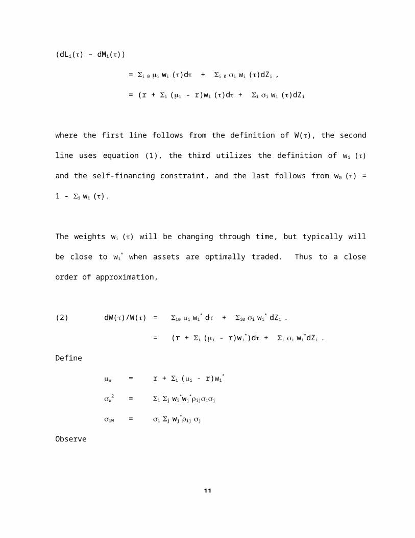
= i 0 i wi ()d + i 0 i wi ()dZi ,

= (r + i (i - r)wi ()d + i i wi ()dZi

where the first line follows from the definition of W(), the second line uses equation (1), the third

utilizes the definition of wi () and the self-financing constraint, and the last follows from w0 () = 1 - i wi

().

The weights wi () will be changing through time, but typically will be close to wi* when assets are

optimally traded. Thus to a close order of approximation,

(2) dW()/W() = i0 i wi* d + i0 i wi

* dZi .

= (r + i (i - r)wi*)d + i i wi

*dZi .

Define

W = r + i (i - r)wi*

W2 = i j wi

*wj*ijij

iW = i j wj*ij j

Observe

W d = E[dW/W]

W2 d = E[(dW/W)2]

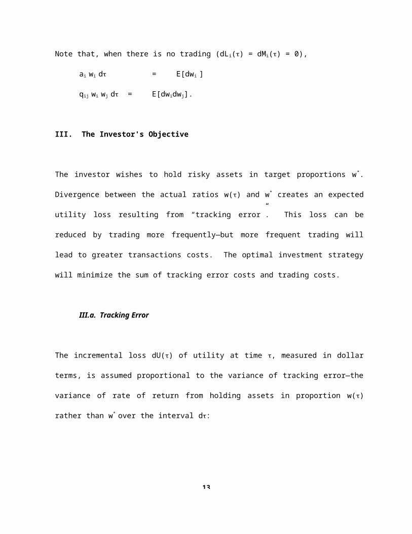
and, when there is no trading (dLi(t) = dMi(t) = 0),

iW d = E[(dSi/Si)(dW/W)]

Since wi() = Si()/W(), it follows from Ito's Lemma that

8

(3) dwi () = (i - W + W2 - iW ) wi d + i wi dZi - (j j wj

* dZj ) wi + wi(),

where wi() = (dLi() – dMi())/W().

The nonnegative process w() is thus right continuous with left-hand limit. Define

ai = i - W + W2 - iW

qij = i j ij - iW - jW + W2,

and let a and Q represent the (1xN) vector and (NxN) matrix with elements ai and qij , respectively.6

Note that, when there is no trading (dLi() = dMi() = 0),

ai wi d = E[dwi ]

qij wi wj d = E[dwidwj].

III. The Investor's Objective

The investor wishes to hold risky assets in target proportions w*. Divergence between the actual ratios

w() and w* creates an expected utility loss resulting from “tracking error”. This loss can be reduced by

trading more frequently—but more frequent trading will lead to greater transactions costs. The optimal

investment strategy will minimize the sum of tracking error costs and trading costs.

III.a. Tracking Error

6 ? Observe that the dynamics of the wi () can vary significantly from the dynamics of the Si (). For example, if there are two positively correlated risky assets whose weights sum to one (implying w0 () = 0), then dwi ()/wi () will be perfectly negatively correlated, i = 1,2.

9

The incremental loss dU() of utility at time , measured in dollar terms, is assumed proportional to the

variance of tracking error—the variance of rate of return from holding assets in proportion w() rather

than w* over the interval d:

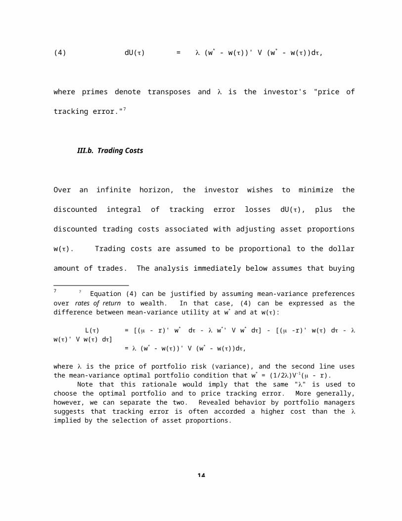
(4) dU() = (w* - w())' V (w* - w())d,

where primes denote transposes and is the investor's "price of tracking error."7

III.b. Trading Costs

Over an infinite horizon, the investor wishes to minimize the discounted integral of tracking error losses

dU(), plus the discounted trading costs associated with adjusting asset proportions w(). Trading costs

are assumed to be proportional to the dollar amount of trades. The analysis immediately below assumes

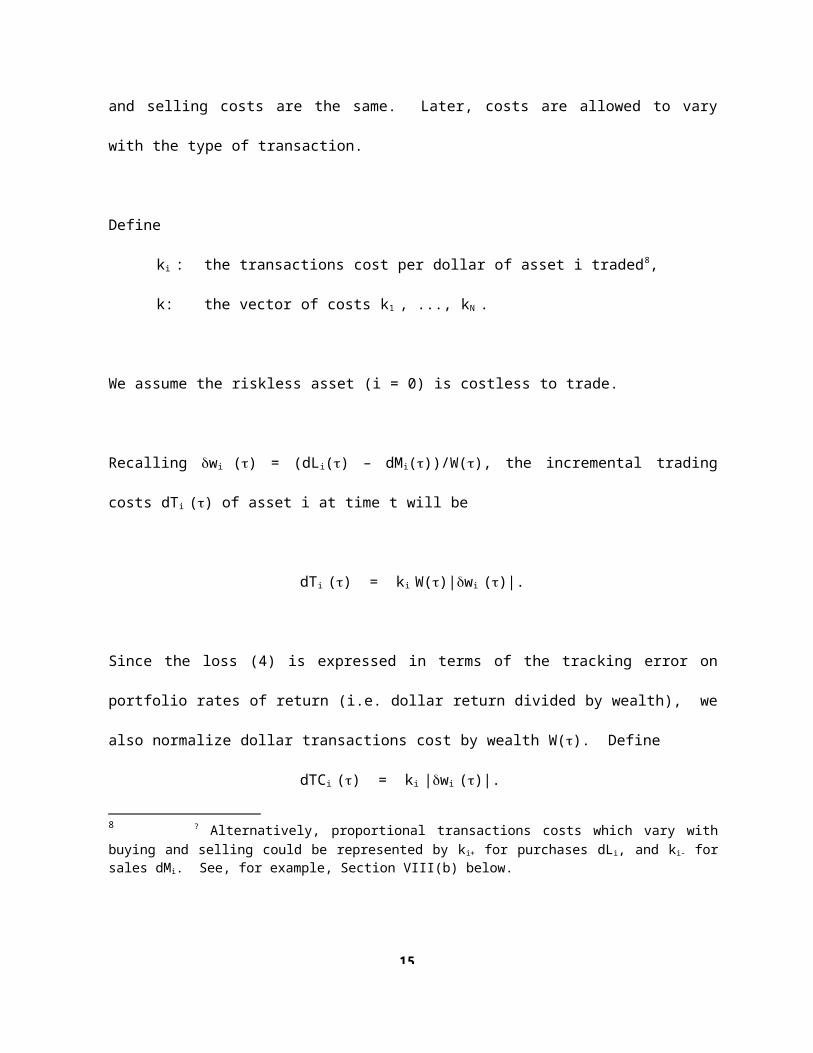
that buying and selling costs are the same. Later, costs are allowed to vary with the type of transaction.

Define

7 ? Equation (4) can be justified by assuming mean-variance preferences over rates of return to wealth. In that case, (4) can be expressed as the difference between mean-variance utility at w* and at w():

L() = [( - r)' w* d - w*' V w* d] - [( -r)' w() d - w()' V w() d] = (w* - w())' V (w* - w())d,

where is the price of portfolio risk (variance), and the second line uses the mean-variance optimal portfolio condition that w* = (1/2)V-1( - r).

Note that this rationale would imply that the same "" is used to choose the optimal portfolio and to price tracking error. More generally, however, we can separate the two. Revealed behavior by portfolio managers suggests that tracking error is often accorded a higher cost than the implied by the selection of asset proportions.

10

ki : the transactions cost per dollar of asset i traded8,

k: the vector of costs k1 , ..., kN .

We assume the riskless asset (i = 0) is costless to trade.

Recalling wi () = (dLi() – dMi())/W(), the incremental trading costs dTi () of asset i at time t will be

dTi () = ki W()|wi ()|.

Since the loss (4) is expressed in terms of the tracking error on portfolio rates of return (i.e. dollar return

divided by wealth), we also normalize dollar transactions cost by wealth W(). Define

dTCi () = ki |wi ()|.

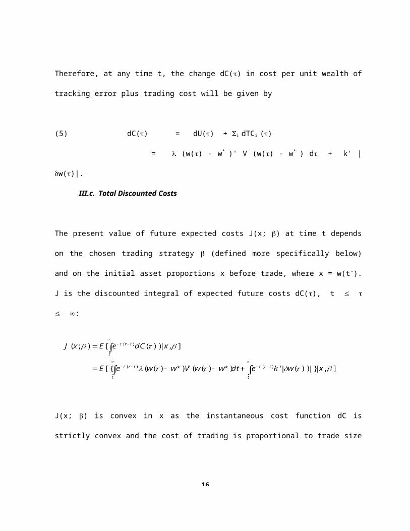
Therefore, at any time t, the change dC() in cost per unit wealth of tracking error plus trading cost will

be given by

(5) dC() = dU() + i dTCi ()

= (w() - w* )' V (w() - w* ) d + k' |w()|.

III.c. Total Discounted Costs

The present value of future expected costs J(x; ) at time t depends on the chosen trading strategy

(defined more specifically below) and on the initial asset proportions x before trade, where x = w(t -). J is 8 ? Alternatively, proportional transactions costs which vary with buying and selling could be represented by ki+ for purchases dLi, and ki- for sales dMi. See, for example, Section VIII(b) below.

11

the discounted integral of expected future costs dC(), t :

J(x; ) is convex in x as the instantaneous cost function dC is strictly convex and the cost of trading is

proportional to trade size (see Harrison and Taksar [1983] and Dumas [1991]).9

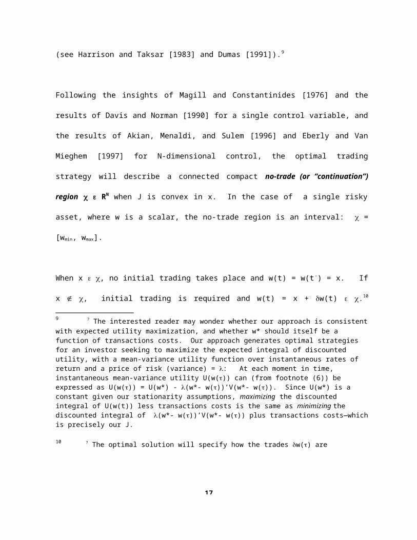
Following the insights of Magill and Constantinides [1976] and the results of Davis and Norman [1990]

for a single control variable, and the results of Akian, Menaldi, and Sulem [1996] and Eberly and Van

Mieghem [1997] for N-dimensional control, the optimal trading strategy will describe a connected

compact no-trade (or “continuation”) region RN when J is convex in x. In the case of a single risky

asset, where w is a scalar, the no-trade region is an interval: = [wmin, wmax].

When x , no initial trading takes place and w(t) = w(t-) = x. If x , initial trading is required and

w(t) = x + w(t) .10 Similar to the results of the previously cited papers, when transactions costs are

9 ? The interested reader may wonder whether our approach is consistent with expected utility maximization, and whether w* should itself be a function of transactions costs. Our approach generates optimal strategies for an investor seeking to maximize the expected integral of discounted utility, with a mean-variance utility function over instantaneous rates of return and a price of risk (variance) = : At each moment in time, instantaneous mean-variance utility U(w()) can (from footnote (6)) be expressed as U(w()) = U(w*) - (w*- w())’V(w*- w()). Since U(w*) is a constant given our stationarity assumptions, maximizing the discounted integral of U(w(t)) less transactions costs is the same as minimizing the discounted integral of (w*- w())’V(w*- w()) plus transactions costs—which is precisely our J.10 ? The optimal solution will specify how the trades w() are determined.

12

proportional, trading will always move asset ratios to a point on the boundary of the no-trade region .

After a potentially large initial trade, subsequent trades will be infinitesimal in size as the (continuous)

diffusion process governing the movement of asset ratios w() will not carry these ratios “far” outside the

boundary before trading back to the boundary occurs. Harrison and Taksar [1983] label this situation as

one of “instantaneous control.”

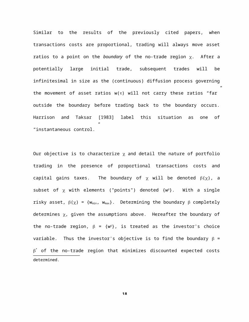
Our objective is to characterize and detail the nature of portfolio trading in the presence of proportional

transactions costs and capital gains taxes. The boundary of will be denoted (), a subset of with

elements ("points") denoted {w}. With a single risky asset, () = {wmin, wmax}. Determining the

boundary completely determines , given the assumptions above. Hereafter the boundary of the no-

trade region, = {w}, is treated as the investor's choice variable. Thus the investor's objective is to find

the boundary = * of the no-trade region that minimizes discounted expected costs J(x; ) .

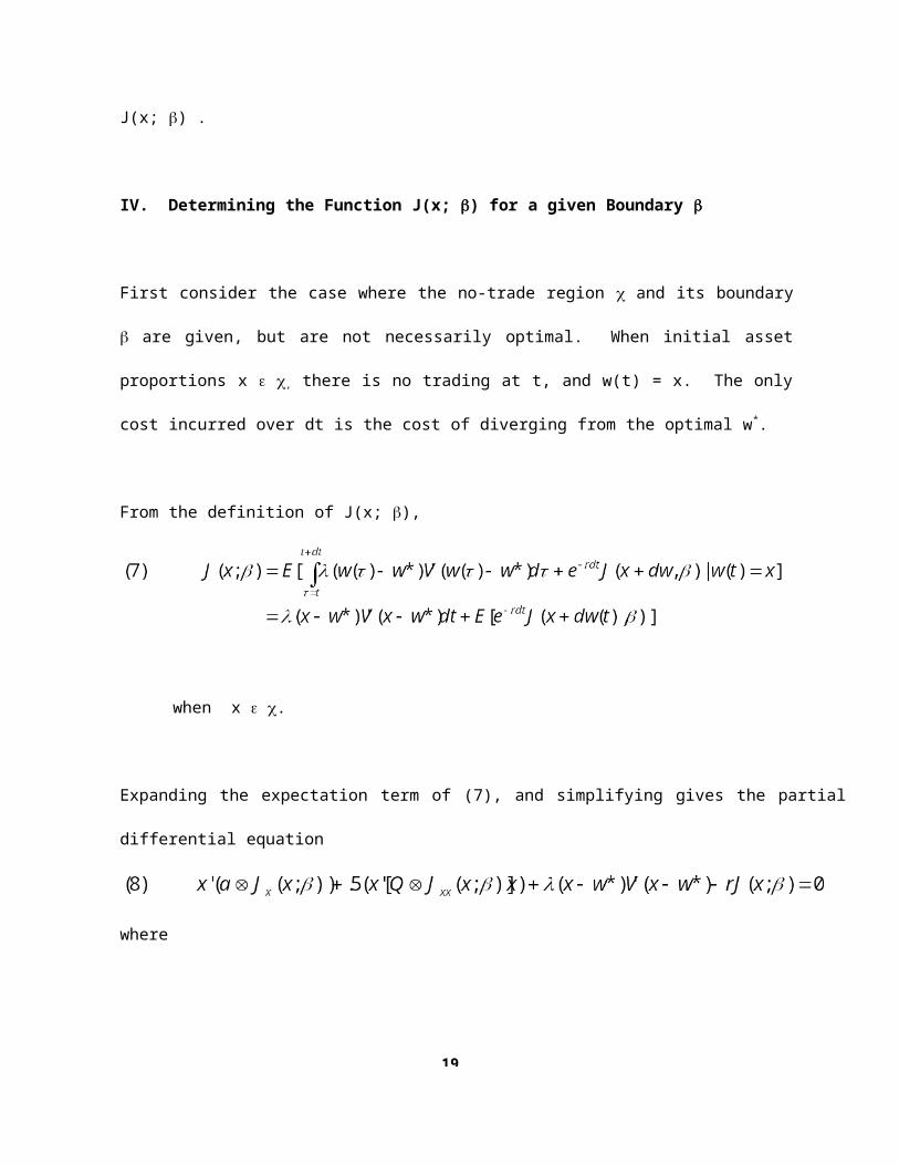
IV. Determining the Function J(x; ) for a given Boundary

First consider the case where the no-trade region and its boundary are given, but are not necessarily

optimal. When initial asset proportions x , there is no trading at t, and w(t) = x. The only cost

incurred over dt is the cost of diverging from the optimal w*.

From the definition of J(x; ),

13

when x .

Expanding the expectation term of (7), and simplifying gives the partial differential equation

where

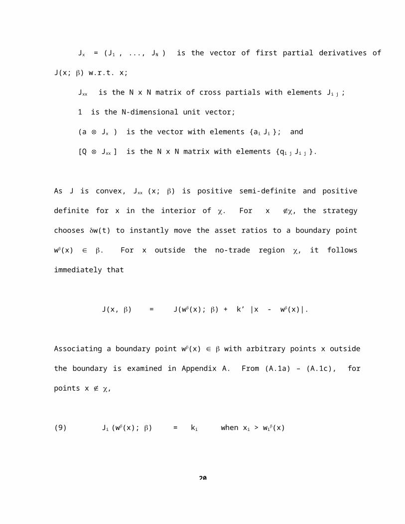
Jx = (J1 , ..., JN ) is the vector of first partial derivatives of J(x; ) w.r.t. x;

Jxx is the N x N matrix of cross partials with elements Ji j ;

1 is the N-dimensional unit vector;

(a Jx ) is the vector with elements {ai Ji }; and

[Q Jxx ] is the N x N matrix with elements {qi j Ji j }.

As J is convex, Jxx (x; ) is positive semi-definite and positive definite for x in the interior of . For x

, the strategy chooses w(t) to instantly move the asset ratios to a boundary point w(x) . For x

outside the no-trade region , it follows immediately that

J(x, ) = J(w(x); ) + k’ |x - w(x)|.

Associating a boundary point w(x) with arbitrary points x outside the boundary is examined in

Appendix A. From (A.1a) – (A.1c), for points x ,

(9) Ji (w(x); ) = ki when xi > wi(x)

= -ki when xi < wi(x)

|Ji (w(x), )| < ki only if xi = wi(x).

14

Conditions (9) hold for arbitrary no-trade regions and their associated boundaries () = {w}. Dumas (1991)

terms these “value matching” conditions. As will be seen below, “most” boundary points will be characterized by

(9) holding for a single i. But the 2N “corner” points on the boundary for which Ji (w; ) = ki , for all i, will be

of considerable computational importance. Let M() denote such points.

Now consider the problem of determining the optimal boundary . The case of a single risky asset (N = 1) builds

from the analysis of Magill and Constantinides [1979], Davis and Norman [1990], and Dumas [1991]. 11 The

general case with an arbitrary number of risky assets N can subsequently be examined.

V. Determining the Optimal No-Trade Region in the Single Risky Asset Case (N = 1)

When there is a single risky asset, the optimal strategy moves x to the boundary point wmin if x < wmin , and to wmax

if x > wmax . (We drop the subscript "1" for the single risky asset case). Therefore w(x) = wmax for all x > wmax,

and w(x) = wmin for all x < wmin. Observe that M() = = {wmin, wmax}: every boundary point belongs to M(),

which is not true for N 2. At the boundary points when wmin and wmax , it follows from (9) that

(10) J1(wmin ; wmin ,wmax ) = -k

(11) J1(wmax ; wmin ,wmax ) = k

where Jn (; , ) is the derivative of J with respect to the nth argument.12 In the single risky asset case, 11 ? Our one-dimensional case differs from Dumas in that the dynamics (3) of the asset weight w follows a logarithmic Brownian motion. It differs from Constantinides in the form of the loss function.12 ? Dumas [1991] shows that these conditions are not smooth-pasting optimality

15

equation (8) is an ordinary differential equation with solution

(12)

where c11 and c12 are uniquely determined as

(13) c11 = (-a + Q/2 + [(a-Q/2)2 + 2Qr].5)/Q;

c12 = (-a + Q/2 - [(a-Q/2)2 + 2Qr].5)/Q,

where from (3)

a = (1 - w*)( - r - 2w*); Q = 2 (1 - w*)2

For a given = {wmin, wmax}, the constants C1 and C2 are determined by the boundary conditions (10) and

(11). The optimal boundary * = {w*min, w*

max} is determined by the "super contact" conditions, which

require that J(x; wmin , wmax ) be minimized w.r.t. wmin and wmax . This provides the two final conditions

needed for optimization, that at the optimal wmin and wmax

(14) J2(wmin ; wmin , wmax ) = 0,

(15) J3(wmax ; wmin , wmax ) = 0.

Following Dumas [1991], it can in turn be shown that these conditions imply

(16) J11 (wmin ; wmin , wmax ) = 0,

(17) J11 (wmax ; wmin , wmax ) = 0.

conditions, but rather the limit of a "value matching" condition. The conditions (sometimes termed “super contact”) associated with the optimal boundary * are given by (16) and (17).

16

Solving (8) subject to the conditions (10), (11), (16), and (17) generates solutions for the optimal strategy

parameters w*min and w*

max , and for the constants C1 and C2 of equation (12), thereby uniquely

determining J(x; * ) = J(x; w*min , w*

max ).

VI. Determining the Optimal No-Trade Region with Multiple Risky Assets (N 2)

The solution to the (partial) differential equation (8) is much more difficult when N 2, since the

boundary set is now described by an infinite number of points rather than the two points {wmin , wmax ).

From equations (A.1a) – (A.1c), recall that at every boundary point w,

(18) |Ji (w, )| ki , i = 1, ..., N,

with equality holding for at least one i. In addition, the maximizing conditions equivalent to (16) and

(17) are that whenever |Ji (w; )| = ki , then

(19) Ji i (w; ) = 0.

When N 2, we are unaware of closed form solutions to equation (8) that satisfy conditions (18) and

(19) at all points of the boundary = {w} of the no-trade region. So we turn now to finding an

approximation of the optimal strategy, which we term the quasi-optimal strategy.

17

VI(a). Determining A Quasi-Optimal No-Trade Region

Our strategy is to find a quasi-optimal solution JA(x; B) which satisfies the p.d.e. equation (8), and

which satisfies conditions (18) and (19) , with JA replacing J, at a finite set of boundary points B. Given

JA, we can then construct the remaining boundary points between these points B by an algorithm

described in Appendix D.13 In general, these in-between boundary points will be constructed to satisfy

either (18) or (19), but will not (except by chance) satisfy both. We develop a measure of how well this

quasi-optimal solution approximates an exact solution, and show that it will be highly accurate for

realistic choices of parameters. Clearly the quasi-optimal function JA(x; B) will depend on the choice of

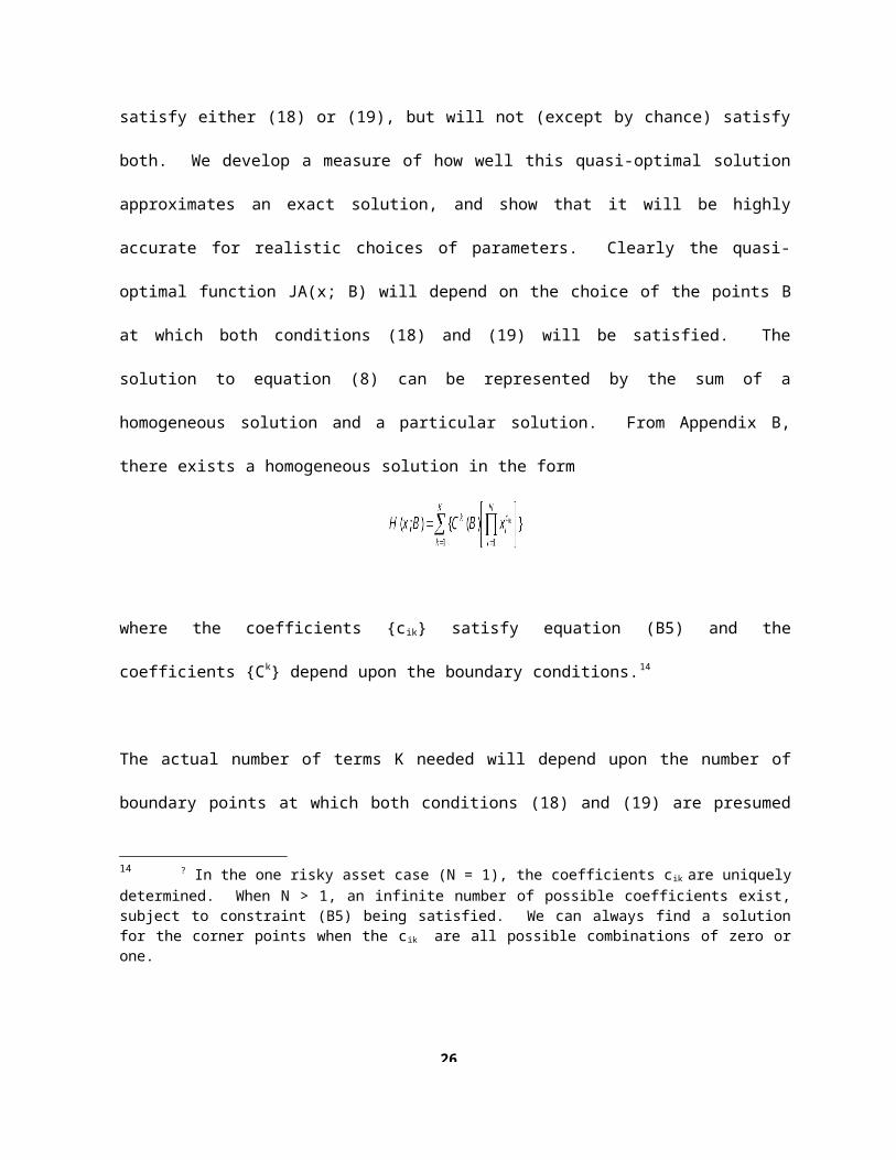
the points B at which both conditions (18) and (19) will be satisfied. The solution to equation (8) can be

represented by the sum of a homogeneous solution and a particular solution. From Appendix B, there

exists a homogeneous solution in the form

where the coefficients {cik} satisfy equation (B5) and the coefficients {Ck} depend upon the boundary

conditions.14

The actual number of terms K needed will depend upon the number of boundary points at which both

conditions (18) and (19) are presumed to be satisfied. A natural set of boundary points B are the 2 N

13 ? Since there are only two boundary points when N = 1 (B = {wmin , wmax }), it follows immediately that the quasi-optimal solution is the fully optimal solution in this case.14 ? In the one risky asset case (N = 1), the coefficients c ik are uniquely determined. When N > 1, an infinite number of possible coefficients exist, subject to constraint (B5) being satisfied. We can always find a solution for the corner points when the c ik are all possible combinations of zero or one.

18

“corner” points where conditions (18) hold with equality for all i, as well as conditions (19). Each corner

point has N dimensions, so there are 2N N variables characterizing the points wB B to be determined. In

addition, we must determine the K constants {Ck} in the homogeneous solution. The total number of

variables to be determined therefore is 2N N + K.

The equations to be satisfied at each of the 2N corner points are the N equations (18)--which hold with

equality at wB B--and the N equations (19). Thus 2N conditions must hold at each of the 2N points, for

a total of 2N+1N equations. For the number of equations to equal the number of unknowns, it follows

that

K = 2NN. We introduce this number of power functions in the homogeneous term (B.2), where the

exponents {ci k } of each function k = 1, …, K satisfy equation (B.5). A particular solution exists of form

(B.9) in Appendix B. The quasi-optimal function JA(x; B) is given by the sum of the homogeneous

solution and the particular solution, satisfying the equations (18) with equality and (19) at the boundary

corner points wB B. These boundary conditions jointly determine the boundary corner points and the

constants {Ck}, k = 1, …, K. Figure 1, discussed in detail in Section IX, locates corner points

{X,Y,Z,V}.

We can use two alternative techniques to construct the remaining boundary points connecting adjacent

corner points wB B, given the function JA(x; B). The first assures that conditions (18) for JA are met

along this boundary; the second assures that conditions (19) are satisfied. Appendix D develops these

algorithms. Let 1* denote the set of boundary points {w1*} determined by the first technique, and 2*

denote the set of boundary points {w2*} determined by the second technique. Because the second

technique proved more tractable computationally, we used it to perform all calculations that follow.

19

The calculation of the boundary 2* using (19) or (D.3) also offers a measure of accuracy of our

approximation. Equation (20) will in general not be satisfied: |JAj (w2*, B)| - kj 0. But for each point

w2* on the boundary we can compute the transactions cost kj (w2*) which would make this term zero, i.e.

kj (w2* ) |JAj (w2*, B)|. For such transactions costs, the quasi-optimal boundary would be fully

optimal, since it would satisfy both conditions (18) and (19). The maximal error over the entire boundary

2* ,

(22) E = Max [ Max [(|kj - kj (w2* )|) ] {w2* , j}

indicates the maximal amount by which transactions costs would have to vary for the quasi-optimal

solution to be the optimal solution. For realistic parameters and modest asset correlations (< .30), this

number is usually small: less than .0005. Thus if the quasi-optimal solution is based on transactions

costs of (say) 1%, then the quasi-optimal solution is exact when transactions costs range appropriately (as

w2* varies) between .95% and 1.05%. Since it is rare to have exact estimates of actual transactions costs,

this range seems tolerable for most practical situations.

But as asset correlations increase, we observe from the examples in Section IX below that errors become

larger—reaching a maximum of .003 when transactions costs are 1 percent. The solution in this case is

exactly optimal only if transactions costs were to vary appropriately between 0.70% and 1.30%, a fairly

broad range. To further reduce errors, a straightforward extension of the approximation method outlined

above is now considered.

20

VI(b). Greater Accuracy of the Quasi-Optimal Solution

The accuracy of the quasi-optimal solution can be improved by finding a JA solution that satisfies the

appropriate conditions (18) and (19) at more than just the corner points.15

In two dimensions, for example, we could require matching the appropriate optimality conditions at a

finite number of points along the boundary segments (XY, YZ, ZV, VX) as well as at the corner points

(X, Y, Z, V). An obvious set of additional points would be the four midpoints of the boundary segments.

We would need an additional four terms in the homogeneous sum (B.2) with exponents satisfying (B.5).

Thus K = 12 in this situation. Matching the boundary conditions at more and more points B leads to

greater and greater accuracy as measured by (22), at the cost of the extra computational requirements as K

rises.

In Section IX, a set of examples examine the differences between solutions with K = 8 and solutions with

K = 12. In the latter solutions, optimality conditions are met at the midpoints of the boundary segments

as well as at the corners. For asset return correlations of 0.2 or less, the no-trade regions are virtually

indistinguishable, with the extreme points {X,Y,Z,V} differing by less than 1% in both dimensions and

the segments joining these points continuing to appear as virtually "straight" lines. However, the

maximal error E defined by (22) falls to about half its previous level. When asset correlation rises to 0.7,

the no-trade regions differ perceptively, and the error of the “corners only” solution (K = 8) rises to .003.

The maximal error falls to .0008 for the K = 12 solution.

15 ? A subset of coordinates for these additional points will be fixed (e.g., the midpoint of a boundary segment joining two corner points). At these points, a subset of conditions (18) and (19) will hold: See Appendix D.

21

VII. Costs, Turnover, and Tracking Error of Optimal Trading Strategies

We have developed techniques for determining the quasi-optimal trading strategies, as expressed by a “no

trade” region with boundary * RN, where * = 1* or 2*, depending on whether technique 1 or 2 is

used to determine the boundary. Now consider a method, first introduced by Leland and Connor [1995]

in the single risky asset case, to estimate the expected present value of transactions costs and annual

expected turnover from following the optimal strategy. We also develop a measure of the expected

tracking error of the optimal strategy.

Consider the function T(x; ) J(x; | = 0) that satisfies the value-matching conditions (18) on the

boundary . This is the expected present cost of the trading strategy with no-trade region determined by

boundary when there is no cost of tracking error, since = 0. Therefore J(x; | = 0) measures the

expected net present value of trading costs when the no-trade region has boundary . By setting = *,

the boundary of the optimal no-trade region for the original problem, the resulting function T(x; *) will

measure the expected net present value of trading costs for the optimal strategy.

When N > 1, there is no known closed form solution for T, so we must use the approximation methods

we used previously. Let TA(x; B) denote the approximate cost function, given the boundary determined

by optimizing JA(x; B). It will satisfy the differential equation (8) with value-matching boundary

conditions as in (18') holding with equality at w B. (It will not satisfy conditions (19), since the

boundary points are optimal for JA, not TA).

22

The solution TA(x; B ) will be the sum of a homogeneous solution to the p.d.e. (8); plus a particular

solution whose coefficients are all zero and hence can be ignored. The homogeneous equation will again

be of the form (B.2), with exponents satisfying (B.5). The 2NN coefficients Ck , k = 1,...,K must be

chosen such that the 2NN value-matching conditions (18') hold with equality at w B.

TA(x; B) therefore gives the discounted expected total trading costs, from = t to infinity, of the quasi-

optimal trading strategy associated with JA(x; B). The annualized expected trading costs ATC are

simply

(23) ATC = r TA(x; B).

If all assets have the same trading costs ki = k, i = 1,..., N, then the annualized expected (one-way)

turnover is

(24) Turnover = ATC / k. 16

The (approximate) expected discounted tracking error cost TE comprises the residual cost: TE = JA -

TA. The annualized tracking error is rTE, and the annualized variance AV associated with this cost is

simply

(25) AV = r TE /

16 ? When ki varies across assets, it is still possible to estimate turnover associated with the quasi-optimal strategy JA(x; B). We construct a function TA*(x; B) as above, but which satisfies the value-matching conditions|TAi*(x; wB)| = k for all i, where is k is an arbitrary constant across all assets i. The solution is the expected discounted transactions costs associated with B, when k is the (common) cost of trading each asset. Annualized turnover is given by rTA*/k.

23

= r (JA - TA) / .

VIII. Optimal Policies with a Single Risky Asset: Some Examples

Consider the following base parameters for asset returns:

Risky asset: = .125

2 = .040

Riskless interest rate: r = .075

Target proportion of risky asset: w* = .60.

We first assume that the cost of selling and buying are identical, and equal to k.

Table I lists the optimal no-trade boundaries {wmin , wmax }, with percent turnover and percent standard

deviation of tracking error in parentheses below, for a range of transactions costs k and cost per unit of

tracking error variance .

Table I examines a range of trading costs, from a low of 0.1% to a high of 10%. For comparison, two

values for the price of tracking error are considered: 1, the value which would also lead a mean-

variance investor to choose a target proportion of (approximately) 60% in the risky asset, given its return

and risk; and 10, a larger value which often seems to characterize the actions of investors trying to track a

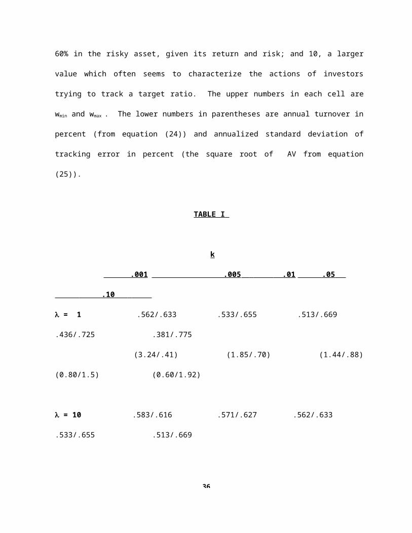
target ratio. The upper numbers in each cell are wmin and wmax . The lower numbers in parentheses are

annual turnover in percent (from equation (24)) and annualized standard deviation of tracking error in

24

percent (the square root of AV from equation (25)).

TABLE I

k

.001 .005 .01 .05 .10

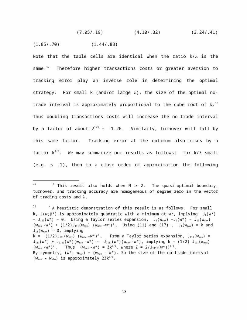
= 1 .562/.633 .533/.655 .513/.669 .436/.725 .381/.775

(3.24/.41) (1.85/.70) (1.44/.88) (0.80/1.5) (0.60/1.92)

= 10 .583/.616 .571/.627 .562/.633 .533/.655 .513/.669

(7.05/.19) (4.10/.32) (3.24/.41) (1.85/.70) (1.44/.88)

Note that the table cells are identical when the ratio k/ is the same.17 Therefore higher transactions costs

or greater aversion to tracking error play an inverse role in determining the optimal strategy. For small k

(and/or large ), the size of the optimal no-trade interval is approximately proportional to the cube root of

k.18 Thus doubling transactions costs will increase the no-trade interval by a factor of about 21/3 = 1.26.

Similarly, turnover will fall by this same factor. Tracking error at the optimum also rises by a factor k1/3.

We may summarize our results as follows: for k/ small (e.g. .1), then to a close order of

17 ? This result also holds when N 2: The quasi-optimal boundary, turnover, and tracking accuracy are homogeneous of degree zero in the vector of trading costs and .

18 ? A heuristic demonstration of this result is as follows. For small k, J(w;*) is approximately quadratic with a minimum at w*, implying J1(w*) = J111(w*) = 0. Using a Taylor series expansion, J1(wmax) –J1(w*) = J11(wmax)(wmax -w*) + (1/2)J111(wmax) (wmax -w*)2 . Using (11) and (17) , J1(wmax) = k and J11(wmax) = 0, implyingk = (1/2)J111(wmax) (wmax -w*)2 . From a Taylor series expansion, J111(wmax) = J111(w*) + J1111(w*)(wmax -w*) = J1111(w*)(wmax -w*), implying k = (1/2) J111(wmax) (wmax -w*)3 . Thus (wmax -w*) = Zk1/3, where Z = 2/J1111(w*))1/3.By symmetry, (w*- wmin) = (wmax – w*). So the size of the no-trade interval (wmax – wmin) is approximately 2Zk1/3.

25

approximation the following propositions hold:

(i) The size of the optimal no-trade interval (wmax - wmin) is

proportional to the cube root of transactions costs.

(ii) Turnover and the size of the optimal no-trade interval

are inversely proportional, implying that turnover is

inversely proportional to the cube root of transactions costs.

(iii) The standard deviation of tracking error and the size of the optimal

no-trade interval are proportional, implying that the standard deviation

of trading error is inversely proportional to the cube root of transactions costs.

Propositions (iii) and (iv) immediately suggest

(iv) The standard deviation of tracking error and turnover are inversely proportional.

Sensitivity to changes in tracking error aversion follows immediately from the invariance of the optimal

strategy for constant k/., implying a change in has the same effect as a change in (1/k).

VIII(a). The Effect of a “Turnover Tax” on Optimal Trading Volume

The results above can be used to assess the impact of proposed taxes on trading by funds seeking to keep

26

assets in given proportions. If other trading costs averaged 0.5%, a 2% tax on portfolio trades, raising

total costs to 2.5%, would reduce trading volume from optimal rebalancing by (1-(.005/.025)1/3), or 42%.

VIII(b). Asymmetric Buying/Selling Costs and Optimal Strategies

in the Presence of Capital Gains Taxes

We now examine the case where the cost of selling (ks ) differs from the cost of buying

(kb ). These costs may differ simply because of market conditions, or because there are capital gains taxes

associated with selling. How does the presence of capital gains taxes, and therefore of asymmetric selling

and buying costs, affect the optimal trading strategy?19

Assume that selling incurs capital gains taxes (e.g. ks = .10, i.e. half the sales price is taxable at a 20%

rate), whereas buying incurs only a trading cost (e.g. kb = .01). Consider the following conjecture: the

optimal strategy is to choose wmax as in the case when both buying and selling costs are .10, and wmin as in

the case when both are .01. If = 10, from Table 1 this would imply

wmax = .669, wmin = .562.

But this conjecture is incorrect. When we solve for the optimal policy with the boundary conditions

J1(wmin; wmin, wmax) = -kb,

19 ? Since the time horizon is infinite, capital gains taxes can be avoided if assets are never sold. Some caution is needed in extending our results to capital gains. First, we assume that capital losses are immediately realized and assets are replaced by repurchasing the (equivalent of) the current position. (This ignores wash sale rules.) Second, our stationary model assumes that capital gains tax rates will remain constant for future asset sales. (Note that the dynamics of buying and selling could change the average cost basis and hence the effective tax rate on sales revenue). The assumption of constant selling costs also precludes a difference between short- and long-term capital gains which Constantinides [1984] showed could create an additional reason for realizing long-term gains.

27

J1(wmax; wmin, wmax) = ks,

plus the optimizing conditions (16) and (17), we find

wmax = .661, wmin = .534.

While the upper trade ratio wmax is similar to that when both trading costs are 10%, the lower trade ratio

wmin is substantially lower than that when both trading costs are 1%. The reason for this becomes clear:

the probability of incurring capital gains in the long run depends (roughly) on the distance between the

midpoint of the no-trade interval and the upper boundary. By lowering the lower boundary of the no-

trade interval, this distance can be increased while keeping the average exposure closer to w*.20

Because wmin is a decreasing function of the capital gains tax rate, an investor commencing with a cash-

only position should initially invest less in the risky asset (to a level wmin ) as the tax rate rises. In the

long run, however, the average risky asset proportion will approximate w* when the optimal strategy is

followed.

Our results should be contrasted with those of Constantinides [1983], who argues that capital gains never

should be realized. But this conclusion presumes that investors can sell short to offset long positions

("shorting the box") in order to avoid realizing capital gains. When this is not possible, the

diversification arguments that are important here cannot be ignored: some capital gains must be realized

20 ? Even if the cost of buying were zero, it would still not be optimal to buy whenever w < w * , if the cost of selling is positive. If kb = 0, and ks = .10, the optimal trading strategy for the example above would be wmin = .536. wmax = .660.

28

to keep tracking error within bounds. Even if shorting the box or a highly correlated security is possible,

it is generally expensive. Synthetically "selling" the original security using these techniques can be

incorporated in our analysis, using their (high) transactions cost rather than the (even higher) capital gains

costs.

VIII(c). Turnover of the Optimal Strategy vs. Periodic Rebalancing

Consider now rebalancing periodically at a time interval t. At the end of each rebalancing period, the

random asset proportions w(t + t) are readjusted back to the desired proportions w*. For equal tracking

error, we are interested in the turnover associated with this strategy relative to the optimal strategy

considered above.

Appendix C gives formulae for the average annual tracking error and turnover associated with a periodic

rebalancing strategy, when there is a single risky asset.

Consider the example from above with w* = .60 and 2 = .04. From Table I, with = 10 and k = .01 (or

equivalently, = 1 and k = .001), annual tracking error standard deviation is 0.41%. Using formula (C5),

setting t = 0.357 (rebalancing approximately three times per year) gives an identical tracking error. But

plugging this value of t into (C7) gives an expected annual turnover of 6.36%, in comparison with the

optimal strategy's turnover of 3.24%. Thus optimal trading reduces turnover by 49%. Comparisons with

other cells in Table I give similar savings of about 50%.

IX. Optimal Policies with a Multiple Risky Assets: Some Examples

29

We now find quasi-optimal trading strategies for the case with two risky assets plus a riskless asset.

While higher-dimensional examples could be constructed with the techniques of Section VII above, they

are numerically intensive and most salient points can be seen in the two risky asset case.

We consider first a symmetric “base” case, with

Risky assets: 1 = 2 = .125

12 = 2

2 = .040

= .200

Riskless interest rate: r = .075

Target proportions of risky assets: w1* = w2

* = .40

Transactions costs: k1 = k2 = .01

Tracking error aversion: = 1.30

The tracking error aversion factor of 1.30 is chosen to equal the variance aversion of the investor

choosing optimally to invest 40% in each risky asset, given the distribution of returns in the base case

above. Alternatively, we later allow the tracking error aversion factor to exceed the investor’s variance

aversion (see footnote 5).

Figure 1 shows the no-trade region for this using the “corners only” (K = 8) solution. The corner point

coordinates are X = {.462, .462}, Y = {.478, .322}, Z = {.332, .332}, and V = {.322, .478}. Turnover is

3.2% and the standard deviation of tracking error is 1.13% per year. The K = 12 solution differs by no

30

more than .001 in any coordinate, and is not shown here.

Although the segments XY, YZ, etc. appear to be linear, they are not exactly. This would be the case

only if JA(x; B) were a quadratic function in the interior of . Nonetheless, once the boundary points

{X,Y,Z,V } have been found, "connecting the dots" seems a reasonable approximation for most

parameter choices.

The quasi-optimal policy is not fully optimal, as discussed above. Since we constructed the boundary

segments XY, YZ, etc. using the conditions JA11(w, B) = 0, JA22(w, B) = 0, etc., we can measure the

error using equation (22), which determines the maximal absolute error |JAi - ki| along the entire

boundary. Figure 1A shows the error along the boundary XY, where w2 varies from Y2 = .332 to X2

= .462. Figure 1B shows the error along the boundary ZY, where w1 varies from Z1 = .332 to Y1 = .478.

The maximal error is approximately .0003, or about 3% of the 1% transactions cost. (Maximal errors

along the other segments ZV and VX are similar.) We conclude that the quasi-optimal strategy would be

fully optimal if transactions costs ranged appropriately between 0.97% and 1.03% along the boundary *.

The K = 12 solution gives even tighter bounds.

When = 10, the no-trade region shrinks to x = {.432, .432}, y = {.438, .361}, z = {.367. .367}, and v =

{.361, .438}.21 Turnover rises to 6.8% and the standard deviation of tracking error falls to 0.56% per

year.

Increasing the correlation between the assets to 0.7 increases the "skewness" of the no-trade region, as

21 21 We continue to assume that w* = (.40, .40). Thus the aversion to tracking error in this case is higher than the aversion to risk which determined the optimal investment proportions. See footnote 5.

31

indicated in the K = 8 solution in Figure 2.22 Maximal errors, however, are substantially larger using the

K = 8 solution. As can be seen in Figures 2A and 2B, these errors reach .003, roughly a third of the

actual transactions costs of 1%. Figure 2(i) illustrates the no-trade region using the K = 12 solution. It is

even more “skewed” than the K = 8 solution. Figures 2A(i) and 2B(i) show that maximal errors are

reduced to .0008, or 8% of the actual transactions costs. Note that even more accuracy could be achieved

by matching the optimality conditions (18) and (19) at even more points along the boundaries—at the

cost of increasing K and computational complexity.

When transactions costs for all risky assets are scaled by a factor , the size of the no-trade region is

approximately proportional to 1/3, as in Proposition (i) for the single risky asset case. Turnover and

tracking error also behave in the fashion outlined by Propositions (ii)-(iv) above.

Not surprisingly, reducing transactions costs of a particular risky asset will shrink the size of the no-trade

region in that dimension. Less obvious is the fact that the no-trade interval will shift for assets whose

transactions costs remain unchanged.

Figure 3 illustrates the case where the trading cost of asset 2 falls to 0.1 percent. 23 Other parameters

remain as in the base case. The optimal no-trade region has corner points X = {.471, .421}, Y =

{.473, .360}, Z = {.324. .378}, and V = {.323, .443}. Contrast the point Z here with Z = (.367, .367),

22 22 We keep the investor’s aversion to variance of tracking error at = 1.30 for purposes of comparison . This tracking error aversion parameter was initially selected because it was also consistent with the risk aversion towards portfolio variance of a mean-variance investor choosing w* = (.40, .40), given the base case distribution. Note, however, that a different risk aversion to portfolio variance would be required for the investor to keep w* = (.40, .40) given the new distribution of asset returns, with higher correlation. See also footnote 5.

23 ? We use K = 12 for greater accuracy.

32

optimal when transactions costs are both 1 percent. As expected, from a start with zero holdings of both

risky assets, more of asset 2 should be bought initially since its transactions costs are lower. But less of

asset 1 should be bought, reflecting the positive correlation of the two assets. Positive correlation implies

that they are (partial) “substitutes.” Buying more of the less-costly asset permits a smaller purchase of the

more-costly asset. This illustrates the dependency of the no-trade region in one dimension upon

transactions costs in other dimensions.

X. The Effect of Transactions Costs on Initial Asset Investments

Consider an investment fund which initially has cash holdings only. It wishes to invest in two assets with

means and variances as given in the base case example of Section IX. The optimal no-trade region is

illustrated in Figure 1.

How do transactions costs affect initial asset investments? Because the initial allocation x = (0, 0) is in

Region V, the initial investments will move asset proportions to the point Z = (.332, .332). When

transactions costs are equal, equal investment will occur in both assets, but less than the desired

proportions (.40, .40). Since initial investment starts at a lower level than desired, the average asset

exposure over a short period of time will be less than 40 percent to each asset. Only as the time horizon

becomes infinite will average investment proportions approach 40 percent each.

Figure 3 illustrates the case with asset correlation 0.7, and transactions costs of the two assets are 1

percent and 0.1 percent, respectively. The aversion to tracking error remains at = 1.30. The no-trade

region is computed with K = 12, and errors are given in Figures 3A and 3B.

33

Starting from an all-cash position, the optimal strategy is to purchase initial fractions given by the point

Z = (.331, .412). Not surprisingly, the amount of asset 1, the high-cost asset, is scaled back substantially

from the ideal 40% proportion. But the initial investment in asset 2, the low-trading-cost asset, is 41.2%,

which exceeds the desired proportion of 40%. The presence of trading costs can lead to a higher initial

purchase of an asset. In the example above, it is optimal to purchase more of the low-cost asset 1 to

replace the lesser amount of asset 2 because the assets are highly correlated and therefore act as

substitutes. In the long run, of course, the average asset proportions will approximate their desired

proportions when the optimal trading strategy is followed.

A currently-popular technique for dealing with transactions costs is to decrease the mean rate of return on

assets, in proportion to their transactions costs. This strategy yields allocation fractions that are

permanently less than target levels.24 And an investor would never make an initial investment that

exceeds the ideal target proportion—although that is required by the optimal policy in Figure 3. The

mean-adjustment technique clearly has important shortcomings, and will be costly to follow relative to

the optimal strategy.

XI. Extensions

XI(a). Nonconstant Target Proportions

24 ? The actual trading strategy, after these “adjusted” target allocations are initially established, is not articulated. If actual proportions are returned to the adjusted targets on a periodic basis, further inefficiencies result as in Section VIII(c).

34

Our analysis has examined the case where dw/w moves relative to a fixed target w*. But the analysis

could be extended to cases where the target w* itself follows a stochastic process. For example, say wi* =

wi*(Z()), i = 1,...,N, t, where Z() is a vector of variables following a joint diffusion process. Z()

may include other variables (e.g. macroeconomic factors whose levels follow a diffusion) as well as stock

prices. The vector w() - w*(Z()) will itself follow a diffusion process with mean and volatility

determined by Ito's Lemma. If the process for Z() has time independent parameters, w() - w* (Z()) will

also have time-independent parameters, and our analysis will be directly applicable with the vector a and

the matrix Q of equation (3) being appropriately modified.

Examples of such w*(Z()) processes include the case when the target ratios wi* are functions of

macroeconomic variables (such as aggregate consumption or interest rates) which follow a time-

independent diffusion, or when the target ratios are functions of relative stock price levels. Time-

independent strategies such as constant proportion portfolio insurance (e.g. Black and Jones [1988]) are

also included, but option-replication strategies are not, due to the time dependence of the target delta.

Our analysis could also be extended to alternative time-independent stochastic processes for the risky

asset values Si , for example an Ornstein-Uhlenbeck diffusion process exhibiting mean reversion.

XI(b). Fixed Components of Transactions Costs

Consider now a fixed cost component in addition to a proportional component of transactions costs.

Work by Dixit [1991] suggests that the optimal trading strategy will be characterized by two regions

35

surrounding w*, one nested within the other. The outer boundary will define the no-trade region. The

inner boundary will be the asset levels optimal to trade to, when asset proportions move outside the larger

no-trade boundary. Dixit [1991] shows how to compute outer and inner regions (intervals) in the single

risky asset case. Even in one dimension the determination of outer and inner intervals is not easy, and we

do not pursue the multi-dimensional extension here.

XII. Conclusions

We have considered optimal rebalancing strategies in the presence of proportional transactions costs. For

both single and multiple risky assets, the optimal strategy is characterized by a no-trade region. When

asset proportions lie within this no-trade region, the optimal policy will be to do nothing. When asset

proportions move outside the region, trades should be undertaken to move the asset proportions to an

appropriate point on the no-trade region's boundary. It is not optimal to trade periodically to the target

asset proportions, despite the popularity of such a strategy. The optimal strategy with identical tracking

error reduces expected turnover by almost 50%.

We developed an exact solution for the single risky asset case, following Constantinides [1979] and

others, and then considered policies for the multi-asset case. A technique for obtaining nearly-optimal

strategies was presented. Our examples suggest that the multi-dimensional no-trade boundary consists of

almost-planar surfaces connecting 2N vertices. We showed that optimal strategies almost always require

buying or selling just one risky asset at any trading date. (The risky asset that must be traded will change

stochastically through time).

36

We also developed a technique for estimating the turnover and tracking error associated with both

optimal strategies and traditional periodic rebalancing strategies. This allows investment managers to

consider the tradeoff between turnover and tracking error in choosing their desired strategy, and to

estimate turnover savings in moving from sub-optimal to optimal strategies.

Capital gains (with some caveats) can be included in the analysis. An important conclusion is that the

presence of capital gains not only affects the no-trade region's upper limits, but also importantly affects

the minimum limits. If synthetic selling strategies are not possible, some capital gains will be realized by

the optimal strategy, in contrast with Constantinides [1984].

A number of ad hoc approaches are currently used to determine the impact of transactions costs on the

amount invested in risky sectors. A popular approach is to reduce the mean return of an asset to reflect

its transactions costs.25 This will lead to less investment than the target amount in the asset, both initially

and in the long run. Our analysis suggests that this approach is seriously flawed. While an investor

starting with an all-cash position may optimally invest less than the target amount in an asset with

transactions costs, we found reasonable examples where it is optimal to initially invest more. (Very) long

run average investment ratios will approach the ideal proportions when the optimal policy is followed.

25 25 The typical adjustment suggests reducing the mean by product of the annual turnover rate of the asset, and the fractional trading costs of the asset. This is ad hoc, in that an optimal policy must determine the turnover endogenously.

37

REFERENCES

Akian, M., Menaldi, J. L., and Sulem, A., 1996, “On an Investment-Consumption Model with Transactions Costs," SIAM Journal of Control and Optimization 34, 329-364.

Black, F., and Jones, R., 1988, “Simplifying Portfolio Insurance for Corporate Pension Plans,” Journal of Portfolio Management 14, 33-37.

Connor, G., and H. Leland [1995], “Cash Management for Index Tracking,” Financial Analysts Journal 51.

Constantinides, G., [1979], "Multiperiod Consumption and Investment Behavior with Convex Transactions Costs," Management Science 25, 1127-1137.

Constantinides, G., [1984], "Optimal Stock Trading with Personal Taxes," Journal of Financial Economics 13, 65-89.

Constantinides, G. [1986], "Capital Market Equilibrium with Transactions Costs," Journal of Political Economy 94, 842-862.

Davis, M., and Norman, A., [1990], "Portfolio Selection with Transaction Costs," Mathematics of Operations Research 15, 676-713.

Dixit, A. [1991], "A Simplified Treatment of Some Results Concerning Regulated Brownian Motion," Journal of Economic Dynamics and Control 15, 657-674.

Dixit, A. [1997], “Investment and Employment Dynamics in the Short Run and the Long Run,” OxfordEconomic Papers 49, 1-20.

Dumas, B. [1991], "Super Contact and Related Optimality Conditions", Journal of Economic Dynamics and Control 15, 675-686.

Eberly, J., and Van Mieghem, J. [1997], “Multi-factor Dynamic Investment Under Uncertainty,” Journal of Economic Theory 75, 345-387.

Grinold, R., and Kahn, R., 1995, Active Portfolio Management: Quantitative Theory and Applications, Phoebus Press.

Harrison, J., Brownian Motion and Stochastic Flow Systems, New York: John Wiley & Sons, 1985.

Harrison, J., and Taksar, M. [1983], “Instantaneous Control of Brownian Motion,” Mathematics of Operations Research 8, 439-453.

Hodges S., and Neuberger, A. [1989], "Optimal Replication of Contingent Claims Under Transactions Costs," Review of Futures Markets 8, 222-239.

38

Leland, H. [1985], "Option Pricing and Replication with Transactions Costs," Journal of Finance 40, 1283-1302.

Shreve, S., and Soner, H. [1994], “Optimal Investment and Consumption with Transactions Costs,” Annals of Applied Probability 4, 909-962.

Taksar, M., Klass, M., and Assaf, D. [1988], “A Diffusion Model for Optimal Portfolio Selection in thePresence of Brokerage Fees,” Mathematics of Operations Research 13, 277-294.

39

APPENDIX A

Characterizing the Boundary Set

We wish to characterize the set of boundary points w(x) RN to which an arbitrary set of asset proportions x outside of will trade.

The cost of moving from x to an arbitrary point w is k'|x - w|. The optimal boundary point to trade to will be

w(x) = ArgMin {J(w, ) + k'|x - w|} w

As Jww(w, ) is positive (semi-) definite, it follows directly that the optimal w will satisfy the Kuhn-Tucker conditions

(A.1a) Ji(w(x), ) = ki if xi > wi(x)

(A.1b) = -ki if xi < wi(x)

(A.1c) |Ji(w(x), )| < ki only if xi = wi(x)

Figure 1 shows a hypothetical no-trade region and associated boundary when N = 2, and the 4 points {X,Y,Z,V} M() at which {J1 = k1, J2 = k2}. These points in turn define the (curvi-) linear segments XY, YZ, ZV, and VX.

Along the segment XY, J1(w,) = k1 at all points w, and J2(w, ) ranges from +k2 (at w = x) to -k2 (at w = y), with |J2(w, )| < k2 except at the endpoints of the segment. From the first order condition (A.1c), it must be that w2(x) = x2 along the interior of the segment XY.

Thus initial asset proportions x which lie to the right of the boundary segment XY (i.e., points in Region II of Figure 1) will be changed to a point on the segment XY with the same amount of the second risky asset. The optimal trade will sell only risky asset 1, and will not trade risky asset 2. Visually, any initial proportions in Region II will trade to the boundary point that is directly to the left of the original point. Similarly, initial asset proportions x lying in Region VI will buy only asset 1 and will not trade asset 2, while initial asset proportions lying in Region IV (Region VIII) will buy (sell) only asset 2 and will not trade asset 1.

Initial asset holdings in Regions I, III, V, and VII will require that both assets be traded, with resulting post-trade holdings represented by the points X, Y, Z, and V, respectively.

Note that, once the no-trade region is reached, random vibrations of the asset proportions will almost surely lead to the next trade being to some boundary point other than X, Y, Z, or V. Thus almost surely subsequent trades will require only one asset to be traded at any given moment.

40

APPENDIX B

Solution to the Partial Differential Equation (8)

As is standard, we write the solution to the partial differential equation as the sum of a homogenous solution(s) plus a particular solution. From equation (8), the homogeneous term H(x; ) of the solution must satisfy

(B1) x'(a Hx ) + .5 (x' [Q Hxx ]x) - rH = 0

We postulate that functions of the form

(B2)

satisfy equation (B1), for arbitrary constants Ck(), k = 1,...,K, when the exponents {cik} are correctly chosen. Consider an arbitrary term in the sum (B2), denoted Hk, where

(B3)

(We suppress the dependence of Hk and Ck on ).

Let ck denote the vector (c1k, ..., cNk). It readily verified that for any Hk,

(B4) x'(a Hkx) = (a'ck) Hk;

x'(Q Hkxx) x = (ck ' Q ck - i cikqii ) Hk.

Plugging these into (B1) yields the (scalar) quadratic equation in the vector ck:

(B5) a'ck + .5(ck 'Qck - i cikqii ) - r = 0,

a quadratic equation which has two solutions for cik when the remaining N-1 {cjk} (j =/ i) are fixed at arbitrary values. When N = 1, Q is a scalar and there are two solutions to equation (B5):

(B6) c11 = [-(a-Q/2) + ((a-Q/2)2 + 2Qr)0.5]/Q,

41

c12 = [-(a-Q/2) - ((a-Q/2)2 + 2Qr)0.5]/Q,

as we derived in Section V above. Note that K = 2 here.

When N = 2, there are an infinite number of solutions to (B5). We may set c2k at any value, and solve (B5) for two possible values for c1k:

(B7)

Conversely, we could set c1k at any value, and derive two possible values for c2k. In the example in Section VI, we set c21 = c22 = 0, and c23 = c24 = 1 for k = 1, 2, 3, and 4, respectively. We can then use (B7) to deriveFinally, we set c15 = c16 = 0, c17 = c18 = 1, and derive c25,...,c28 in a similar manner.

The homogeneous term H(x, ) is the weighted sum of the Hk functions whose exponents each satisfy

equation (B5), and therefore H will satisfy B5 as well. The weights Ck() will be determined by the boundary conditions.

We seek a particular solution in the form

(B.9) P(w) = 0 + i ixi + i,j ijxixj

which satisfies the partial differential equation (8).

The solution is tedious but straightforward. For example, when N = 2, the coefficients satisfy

(B.10) 0 = (w1* 21

2 + 2w1*w2

*1212 + w2* 22

2)/r

(B8)

42

1 = 2(w1*1

2 + w2*1212)/(a1 - r)

2 = 2(w2*2

2 + w1*1212)/(a2 - r)

11 = -12/(q11 + 2a1 - r)

12 = -1212/(q12 + a1 + a2 - r)

22 = -22/(q22 + 2a2 - r)

The solution to the p.d.e. (8) is the sum of the homogeneous solution and the particular solution, with the coefficients of the homogeneous solution chosen to fit the boundary conditions.

APPENDIX C

C(1). Tracking Error of Periodic Rebalancing

Consider the expected net present value of tracking error in the single risky asset case, where denotes the rebalancing strategy:

(C1)

Assume that the program commences at w(t) = w*, and rebalancing to w* occurs at times {t + t, t + 2t, ... }. t (measured in years) is the rebalancing interval. It follows that

(C2)

From time homogeneity, we may write (C2) as

(C3)

43

or using the formula for the sum of an infinite series,

From (3), w( - t) / w* is lognormal with mean ea(-t) and variance e2a(-t)(eQ(-t) - 1). Therefore

where h1 = a - r; h2 = 2a + Q - r.

Substituting this into (C3) gives

C(2). Trading Required for Periodic Rebalancing

Trading will occur at the end of each rebalancing period, i.e. at t + t, t + 2t, etc., and will restore the risky asset proportion to w*. The expected cost of trading (normalized by wealth W) at the end of each period will equal ET = kE[|w(t + t) - w*|], the expected absolute value of the change in w over the rebalancing period times the cost of trading k. The present value of the first period trading will be e -rtET, and the capitalized value of the trading cost will be T = e -rtET/(1 - ert). Annualized trading cost will be rT.

Thus we must derive the expected absolute move of w() - w* at the end of the rebalancing period t. It can be shown that26

26 ? The author thanks Peter DeMarzo and Hui Ou-Yang for this result.

44

(C6) E[|w(t + t) - w*|] = w* (N(-z1) - N(z1) + eat(N(z2) - N(-z2))),

where N( ) is the cumulative uniform normal distribution, and

z1 = (a - .5Q)t/(Qt)1/2

z2 = z1 + (Qt)1/2.

The discounted expected trading costs T of rebalancing at intervals t is therefore

(C7) T = ke-rt (w* (N(-z1) - N(z1) + eat(N(z2) - N(-z2)))/(1 - e-rt ),

and the expected annualized (one-way) turnover is given by

(C8) Turnover = rT/k.

45

APPENDIX D: CALCULATING THE QUASI-OPTIMAL BOUNDARY GIVEN JA(x; B)

Given the function JA(x; B), the algorithm works as follows. For a given (arbitrarily small) step size i,

consider the vector of values Mi = (-ki, -ki+i, -ki+2i,..., +ki), i = 1,...,N.

Define the product space

and let m -j denote an arbitrary point in M -j . The ith component (i j) of the vector m -j will be denoted

mi, -j . Now choose an arbitrary j, 1 j N. Solve the following equations for x:

(D.1) JAj (x; B) = kj

JAi (x; B) = mi, -j , i = 1, ..., N, i j.

As JA is strictly convex for x, there will be a unique solution x = w(kj , m -j ) for each possible

m -j M -j . There will be another unique solution w(-kj , m -j ) when JAj (x; B) = -kj . The boundary set

will then be given by

= {w = w(kj , m -j )|m -j M -j , j = 1,...,N}.

Note that for all w , the conditions

(D.2) |JAi (w ; B)| ki , i = 1, ..., N

46

will be satisfied, with equality holding for at least one i. Also note that as the steps {i } become small,

the relative number of points w in for which (D.2) holds with equality for i j will become equally

small. In the limit, almost surely conditions (D.2) will hold with strict inequality for i j. From

Appendix A, this in turn implies that only asset j will be traded in moving to the boundary. We conclude

that once we are inside or on the boundary, the quasi-optimal trading strategy will almost surely require

trading no more than one risky asset at any moment. Which asset is traded will vary stochastically

through time.

The second technique for determining the boundary replaces equations (D.1) with

(D.3) JAj j (x; B) = 0,

JAi (x; B) = mi, -j , i = 1, ..., N, i j.

There will be two values of x satisfying (D.3) for each point m-j, corresponding to opposite sides of the

no-trade boundary. The solution set * = {w*} satisfying (D.3) for all {i, j} will be slightly different than

the solution set = {w} satisfying (D.1) except at the points B. However, examples show that the

"patched in" boundaries will be virtually identical. Conditions (D.3) are used to determine the no-trade

boundary in our examples.