Embed Size (px)
Citation preview
UNIT 3 ROUTING
Routing (RIP, OSPF, metrics) – Switch basics – Global Internet (Areas, BGP, IPv6), Multicast
– addresses – multicast routing (DVMRP, PIM)
Routing
Routing is the process of finding the shortest path and delivering the data through shortest path.
DISTANCE VECTOR ROUTING (OR) ROUTING INFORMATION PROTOCOL (OR) BELLMAN-FORD ALGORITHM
ROUTING ALGORITHMS
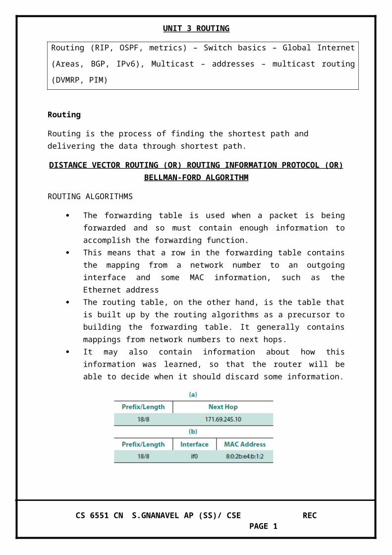
The forwarding table is used when a packet is being forwarded and so must contain enough information to accomplish the forwarding function.
This means that a row in the forwarding table contains the mapping from a network number to an outgoing interface and some MAC information, such as the Ethernet address
The routing table, on the other hand, is the table that is built up by the routing algorithms as a precursor to building the forwarding table. It generally contains mappings from network numbers to next hops.
It may also contain information about how this information was learned, so that the router will be able to decide when it should discard some information.
Example rows from (a) routing and (b) forwarding tables Network as a Graph Routing is, in essence, a problem of graph theory.
The nodes of the graph, labeled A through F, may be either hosts, switches,routers, or networks.
CS 6551 CN S.GNANAVEL AP (SS)/ CSE REC PAGE 1
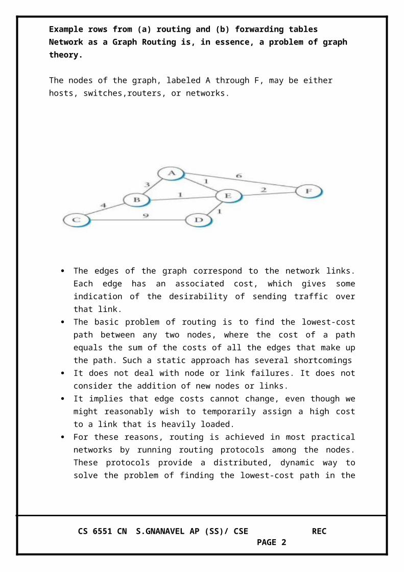
The edges of the graph correspond to the network links. Each edge has an associated cost, which gives some indication of the desirability of sending traffic over that link.
The basic problem of routing is to find the lowest-cost path between any two nodes, where the cost of a path equals the sum of the costs of all the edges that make up the path. Such a static approach has several shortcomings
It does not deal with node or link failures. It does not consider the addition of new nodes or links.
It implies that edge costs cannot change, even though we might reasonably wish to temporarily assign a high cost to a link that is heavily loaded.
For these reasons, routing is achieved in most practical networks by running routing protocols among the nodes. These protocols provide a distributed, dynamic way to solve the problem of finding the lowest-cost path in the presence of link and node failures and changing edge costs.
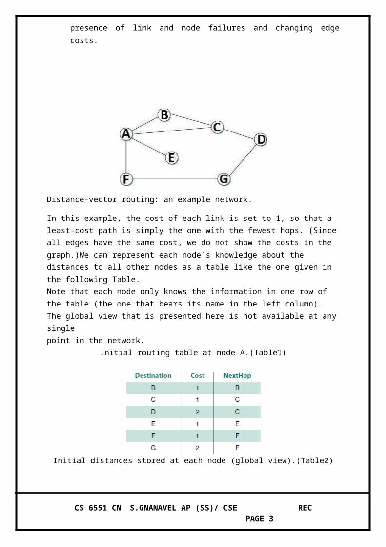
Distance-vector routing: an example network.
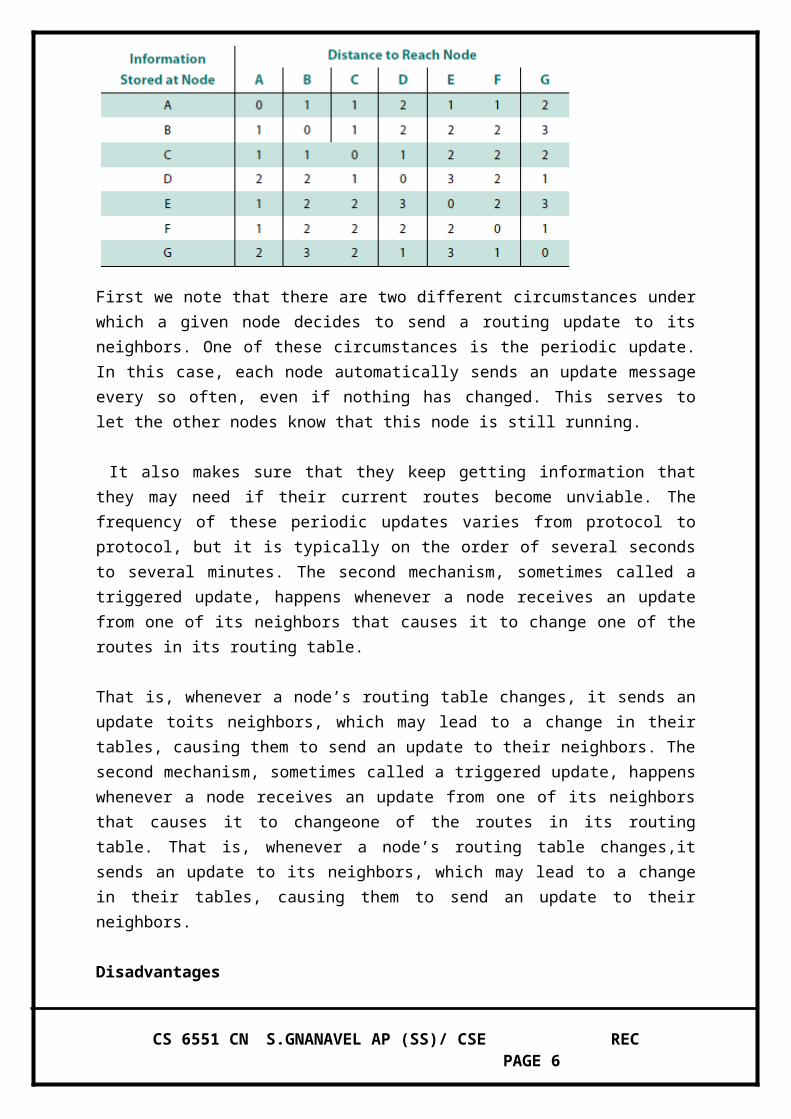
In this example, the cost of each link is set to 1, so that a least-cost path is simply the one with the fewest hops. (Since all edges have the same cost, we do not show the costs in the graph.)We can represent each node’s knowledge about the distances to all other nodes as a table like the one given in the following Table.Note that each node only knows the information in one row of the table (the one that bears its name in the left column). The global view that is presented here is not available at any singlepoint in the network.
Initial routing table at node A.(Table1)
CS 6551 CN S.GNANAVEL AP (SS)/ CSE REC PAGE 2
Initial distances stored at each node (global view).(Table2)
We may consider each row in Table 2 as a list of distances from one node to all other nodes, representing the current beliefs of that node. Initially, each node sets a cost of 1 to its directly connected neighbors and ∞ to all other nodes.Thus, A initially believes that it can reach B in one hop and that D is unreachable. The routing table stored at A reflects this set of beliefs and includes the name of the next hop that A would use to reach any reachable node. Initially, then, A’s routing table would look like Table 1.The next step in distance-vector routing is that every node sends a message to its directly connected neighbors containing its personal list of distances.For example node F tells node A that it can reach node G at a cost of 1; A also knows it can reach F at a cost of 1, so it adds these costs to get the cost of reaching G by means of F.This total cost of 2 is less than the current cost of infinity, so A records that it can reach G at a cost of 2 by going through F. Similarly, A learns from C that D can be reache from C at a cost of 1; it adds this to the cost of reaching C (1) and decides that D can be reached via C at a cost of 2, which is better than the old cost of infinity.At the same time, A learns from C that B can be reached from C at a cost of 1, so it concludes that the cost of reaching B via C is 2. Since this is worse than the current cost of reaching B (1), this new information is ignored.
CS 6551 CN S.GNANAVEL AP (SS)/ CSE REC PAGE 3
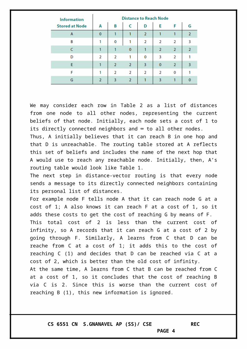
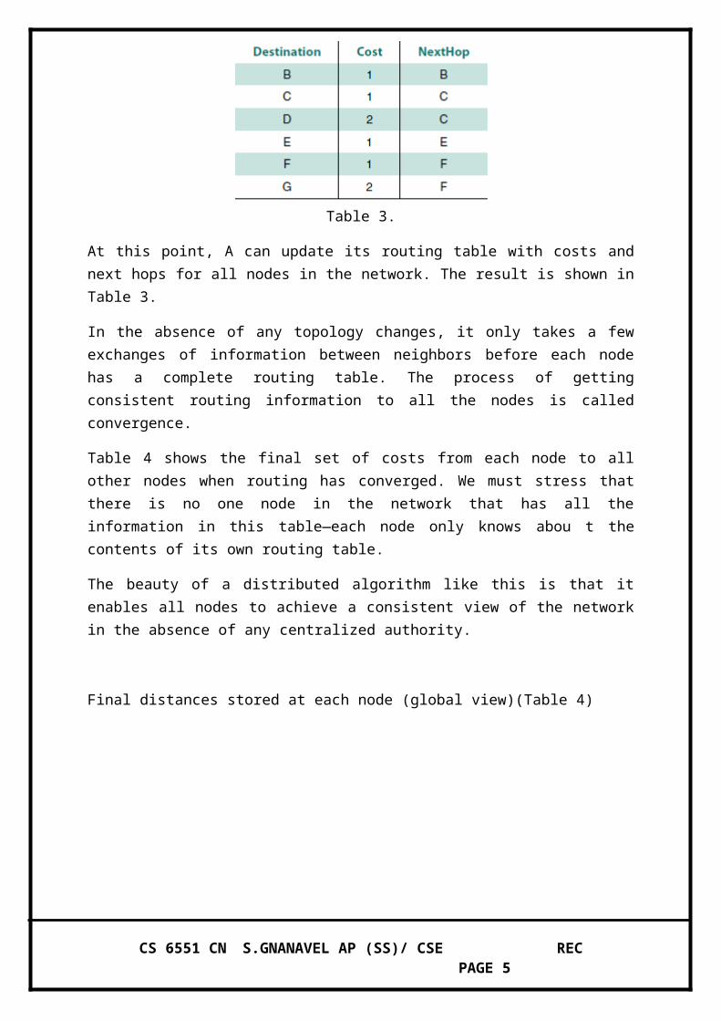
Table 3.
At this point, A can update its routing table with costs and next hops for all nodes in the network. The result is shown in Table 3.
In the absence of any topology changes, it only takes a few exchanges of information between neighbors before each node has a complete routing table. The process of getting consistent routing information to all the nodes is called convergence.
Table 4 shows the final set of costs from each node to all other nodes when routing has converged. We must stress that there is no one node in the network that has all the information in this table—each node only knows abou t the contents of its own routing table.
The beauty of a distributed algorithm like this is that it enables all nodes to achieve a consistent view of the network in the absence of any centralized authority.
Final distances stored at each node (global view)(Table 4)
First we note that there are two different circumstances under which a given node decides to send a routing update to its neighbors. One of these circumstances is the periodic update. In this case, each node automatically sends an update message every so often, even if nothing has changed. This serves to let the other nodes know that this node is still running.
It also makes sure that they keep getting information that they may need if their current routes become unviable. The frequency of these periodic updates varies from protocol to protocol, but it is typically on the order of several seconds to several minutes. The second
CS 6551 CN S.GNANAVEL AP (SS)/ CSE REC PAGE 4
mechanism, sometimes called a triggered update, happens whenever a node receives an update from one of its neighbors that causes it to change one of the routes in its routing table.
That is, whenever a node’s routing table changes, it sends an update toits neighbors, which may lead to a change in their tables, causing them to send an update to their neighbors. The second mechanism, sometimes called a triggered update, happens whenever a node receives an update from one of its neighbors that causes it to changeone of the routes in its routing table. That is, whenever a node’s routing table changes,it sends an update to its neighbors, which may lead to a change in their tables, causing them to send an update to their neighbors.
DisadvantagesThe routing tables for the network do not stabilize. This situation is known as the count-to-infinity problem.One technique to improve the time to stabilize routing is called split horizon.
The idea is that when a node sends a routing update to its neighbors, it does not send those routes it learned from each neighbor back to that neighbor. For example, if B has the route (E, 2, A) in its table, then it knows it must have learned this route from A, and so whenever B sends a routing update to A, it does not include the route (E, 2) in that update.In a stronger variation of split horizon, called split horizon with poison reverse, B actually sends that route back to A, but it puts negative information in the route to ensure that A will not eventually use B to get to E. For example, B sends the route (E, ∞) to A.
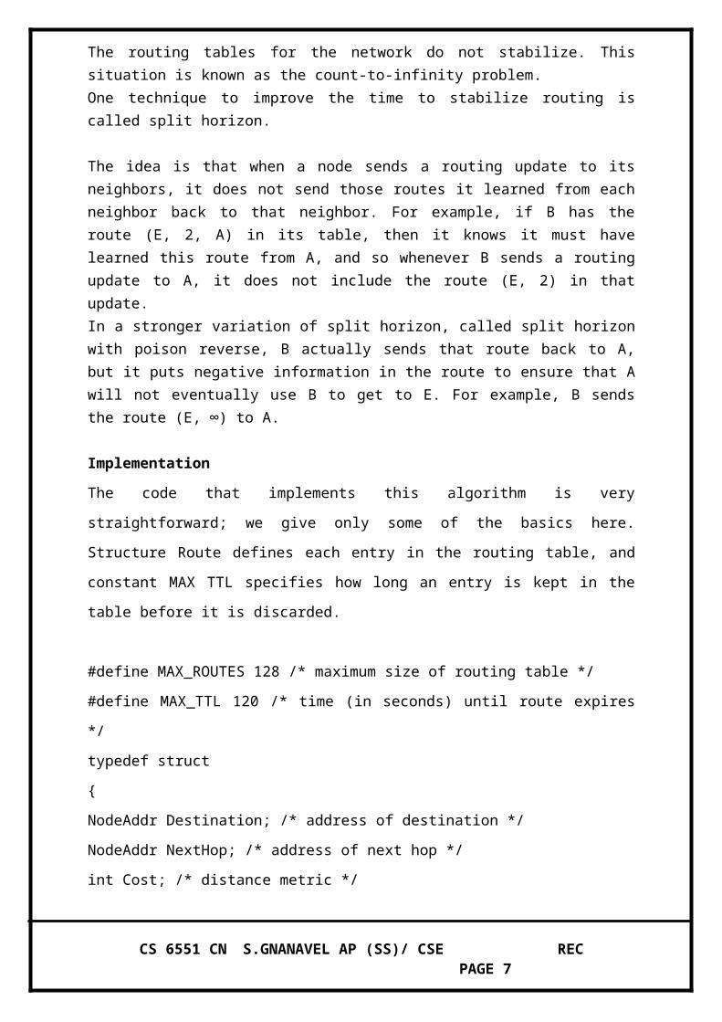
Implementation
The code that implements this algorithm is very straightforward; we give only some of the
basics here. Structure Route defines each entry in the routing table, and constant MAX TTL
specifies how long an entry is kept in the table before it is discarded.
#define MAX_ROUTES 128 /* maximum size of routing table */
#define MAX_TTL 120 /* time (in seconds) until route expires */
typedef struct
{
NodeAddr Destination; /* address of destination */
NodeAddr NextHop; /* address of next hop */
int Cost; /* distance metric */
u_short TTL; /* time to live */
} Route;
int numRoutes = 0;
Route routingTable[MAX_ROUTES];
CS 6551 CN S.GNANAVEL AP (SS)/ CSE REC PAGE 5
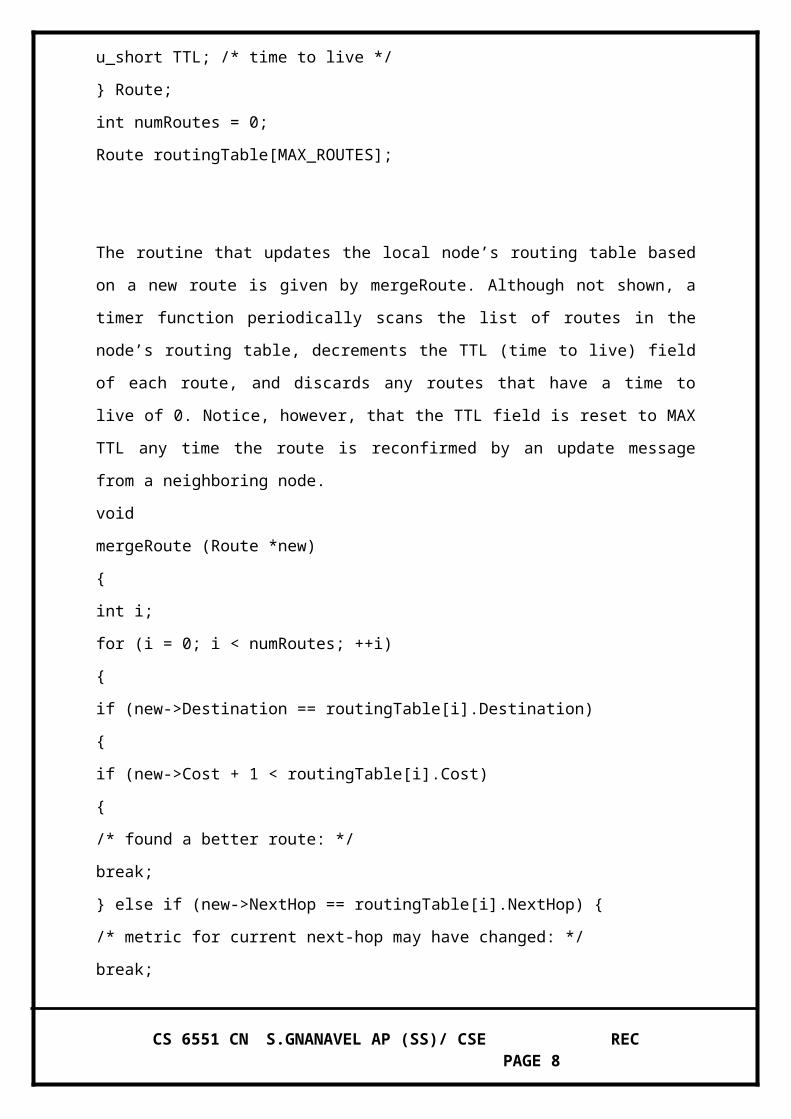
The routine that updates the local node’s routing table based on a new route is given by
mergeRoute. Although not shown, a timer function periodically scans the list of routes in the
node’s routing table, decrements the TTL (time to live) field of each route, and discards any
routes that have a time to live of 0. Notice, however, that the TTL field is reset to MAX TTL
any time the route is reconfirmed by an update message from a neighboring node.
void
mergeRoute (Route *new)
{
int i;
for (i = 0; i < numRoutes; ++i)
{
if (new->Destination == routingTable[i].Destination)
{
if (new->Cost + 1 < routingTable[i].Cost)
{
/* found a better route: */
break;
} else if (new->NextHop == routingTable[i].NextHop) {
/* metric for current next-hop may have changed: */
break;
}
else
{
/* route is uninteresting---just ignore it */
return;
}
}
}
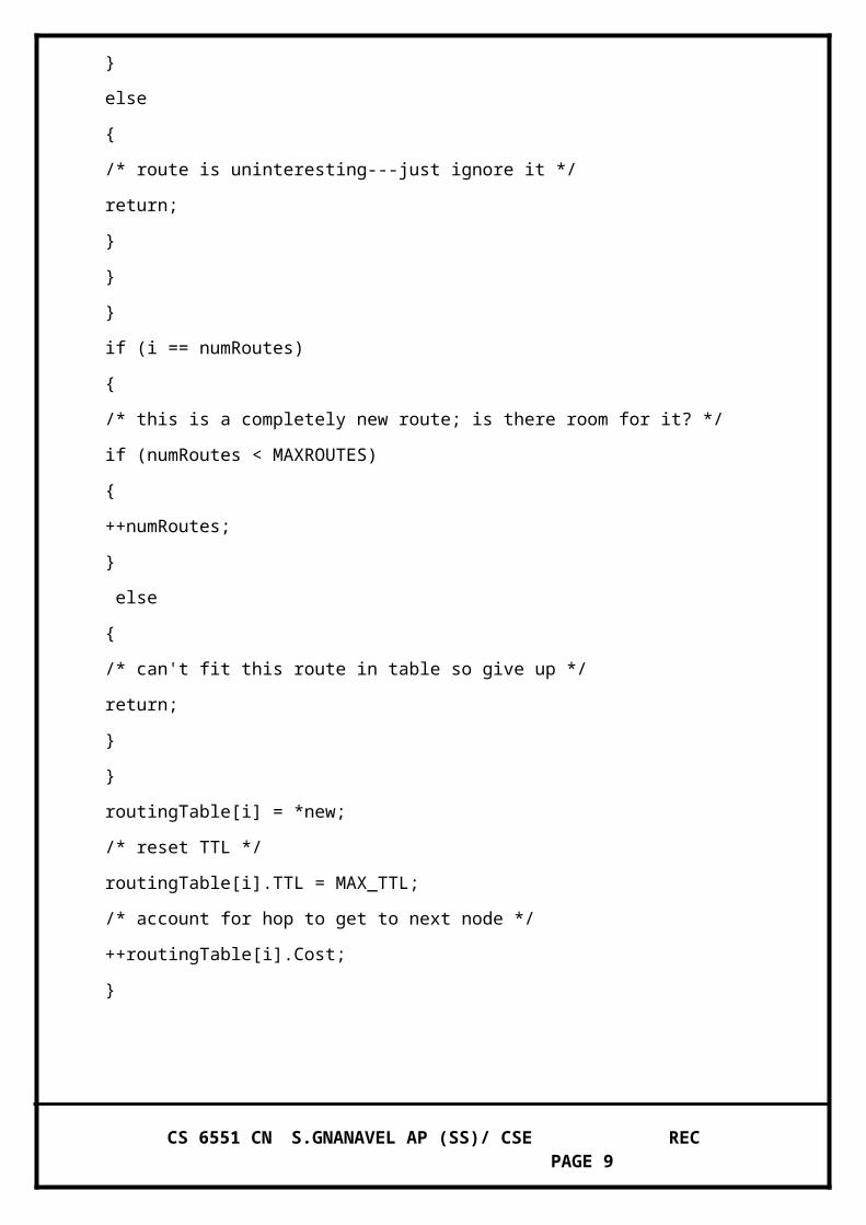
if (i == numRoutes)
{
/* this is a completely new route; is there room for it? */
if (numRoutes < MAXROUTES)
{
++numRoutes;
CS 6551 CN S.GNANAVEL AP (SS)/ CSE REC PAGE 6
}
else
{
/* can't fit this route in table so give up */
return;
}
}
routingTable[i] = *new;
/* reset TTL */
routingTable[i].TTL = MAX_TTL;
/* account for hop to get to next node */
++routingTable[i].Cost;
}
Finally, the procedure updateRoutingTable is the main routine that calls mergeRoute to
incorporate all the routes contained in a routing update that is received from a neighboring
node.
void
updateRoutingTable (Route *newRoute, int numNewRoutes)
{
int i;
for (i=0; i < numNewRoutes; ++i)
{
mergeRoute(&newRoute[i]);
}
}
Routing Information Protocol (RIP)
One of the more widely used routing protocols in IP networks is the Routing Information
Protocol (RIP). Its widespread use in the early days of IP was due in no small part to the fact
that it was distributed along with the popular Berkeley Software Distribution (BSD) version
of Unix, from which many commercial versions of Unix were derived. It is also extremely
simple. RIP is the canonical example of a routing protocol built on the distance-vector
algorithm just described.
Routing protocols in internetworks differ very slightly from the idealized graph model
described above. In an internetwork, the goal of the routers is to learn how to forward packets
CS 6551 CN S.GNANAVEL AP (SS)/ CSE REC PAGE 7
to various networks. Thus, rather than advertising the cost of reaching other routers, the
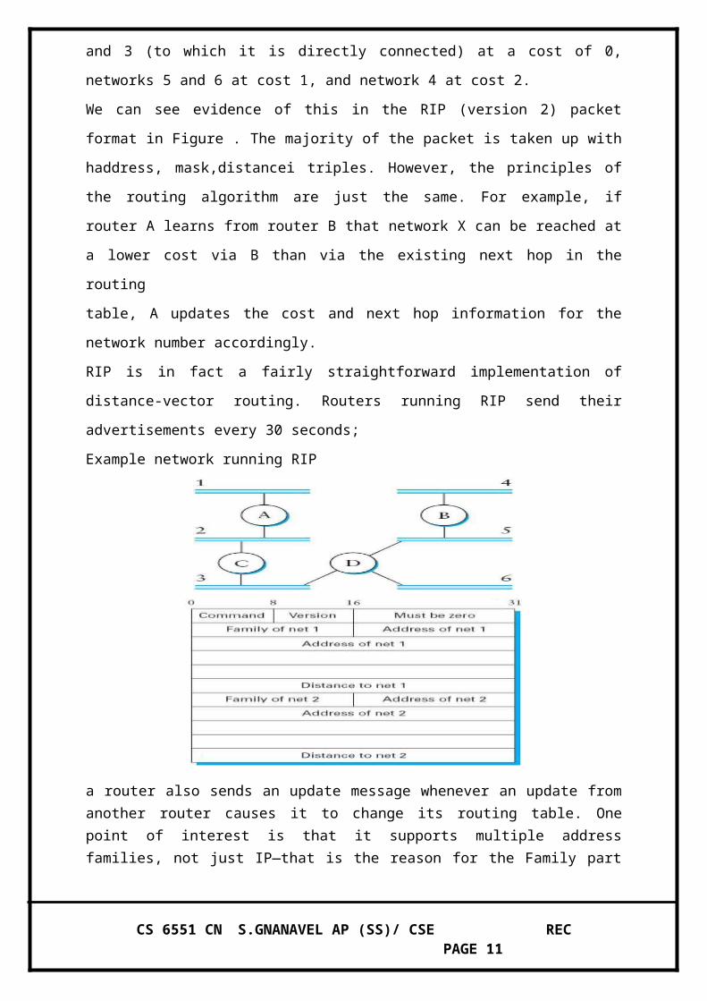
routers advertise the cost of reaching networks. For example, in Figure, router C would
advertise to router A the fact that it can reach networks 2 and 3 (to which it is directly
connected) at a cost of 0, networks 5 and 6 at cost 1, and network 4 at cost 2.
We can see evidence of this in the RIP (version 2) packet format in Figure . The majority of
the packet is taken up with haddress, mask,distancei triples. However, the principles of the
routing algorithm are just the same. For example, if router A learns from router B that
network X can be reached at a lower cost via B than via the existing next hop in the routing
table, A updates the cost and next hop information for the network number accordingly.
RIP is in fact a fairly straightforward implementation of distance-vector routing. Routers
running RIP send their advertisements every 30 seconds;
Example network running RIP
a router also sends an update message whenever an update from another router causes it to change its routing table. One point of interest is that it supports multiple address families, not just IP—that is the reason for the Family part of the advertisements. RIP version 2 (RIPv2) also introduced the subnet masks described in Section 3.2.5, whereas RIP version 1 worked with the old classful addresses of IP.
As we will see below, it is possible to use a range of different metrics or costs for the links in a routing protocol. RIP takes the simplest approach, with all link costs being equal to 1, just as in our example above. Thus, it always tries to find the minimum hop route. Valid distances are 1 through 15, with 16 representing infinity. This also limits RIP to running on fairly small networks—those with no paths longer than 15 hops.
CS 6551 CN S.GNANAVEL AP (SS)/ CSE REC PAGE 8
Link State Routing (OSPF)
Link-state routing is the second major class of intradomain routing protocol. The starting assumptions for link-state routing are rather similar to those for distance vector routing.
Each node is assumed to be capable of finding out the state of the link to its neighbors (up or down) and the cost of each link. Again, we want to provide each node with enough information to enable it to find the least-cost path to any destination.
The basic idea behind link-state protocols is very simple: Every node knows how to reach its directly connected neighbors, and if we make sure that the totality of this knowledge is disseminated to every node, then every node will have enough knowledge of the network to build a complete map of the network.
Thus, link-state routing protocols rely on two mechanisms: reliable dissemination of link-state information, and the calculation of routes from the sum of all the accumulated link-state knowledge.
Reliable Flooding
Reliable flooding is the process of making sure that all the nodes participating in the routing
protocol get a copy of the link-state information from all the other nodes. As the
term―flooding suggests, the basic idea is for a node to send its link-state information out on
all of its directly connected links, with each node that receives this information forwarding it
out on all of its links.This process continues until the information has reached all the nodes in
the network. More precisely, each node creates an update packet, also called a link-state
packet (LSP), that contains the following information.
The ID of the node that created the LSP
A list of directly connected neighbors of that node, with the cost of the link to each
one
A sequence number
A time to live for this packet.
The first two items are needed to enable route calculation; the last two are used to make the
process of flooding the packet to all nodes reliable. Reliability includes making sure that you
have the most recent copy of the information, since there may be multiple, contradictory
LSPs from one node traversing the network
CS 6551 CN S.GNANAVEL AP (SS)/ CSE REC PAGE 9
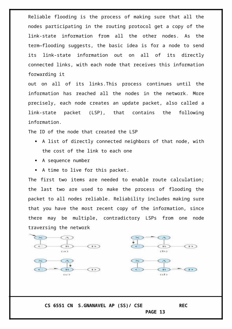
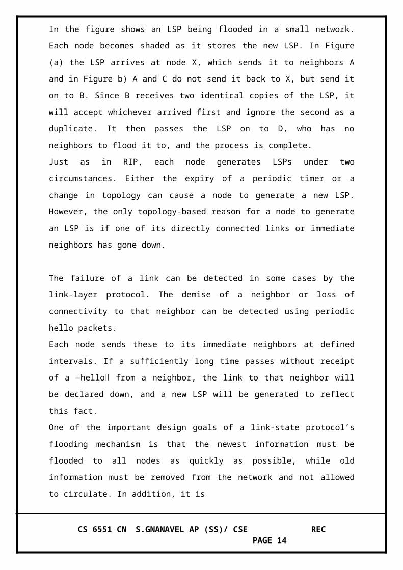
In the figure shows an LSP being flooded in a small network. Each node becomes shaded as
it stores the new LSP. In Figure (a) the LSP arrives at node X, which sends it to neighbors A
and in Figure b) A and C do not send it back to X, but send it on to B. Since B receives two
identical copies of the LSP, it will accept whichever arrived first and ignore the second as a
duplicate. It then passes the LSP on to D, who has no neighbors to flood it to, and the process
is complete.
Just as in RIP, each node generates LSPs under two circumstances. Either the expiry of a
periodic timer or a change in topology can cause a node to generate a new LSP. However, the
only topology-based reason for a node to generate an LSP is if one of its directly connected
links or immediate neighbors has gone down.
The failure of a link can be detected in some cases by the link-layer protocol. The demise of a
neighbor or loss of connectivity to that neighbor can be detected using periodic hello packets.
Each node sends these to its immediate neighbors at defined intervals. If a sufficiently long
time passes without receipt of a ―helloǁ from a neighbor, the link to that neighbor will be
declared down, and a new LSP will be generated to reflect this fact.
One of the important design goals of a link-state protocol’s flooding mechanism is that the
newest information must be flooded to all nodes as quickly as possible, while old information
must be removed from the network and not allowed to circulate. In addition, it is
clearly desirable to minimize the total amount of routing traffic that is sent around the
network after all, this is just overhead from the perspective of those who actually use the
network for their applications. The next few paragraphs describe some of the ways that these
goals are accomplished.
One easy way to reduce overhead is to avoid generating LSPs unless absolutely necessary.
This can be done by using very long timers often on the order of hours for the periodic
generation of LSPs. Given that the flooding protocol is truly reliable when topology Changes,
it is safe to assume that messages saying nothing has changed do not need to be sent very
often.
LSPs also carry a time to live. This is used to ensure that old link-state information is
eventually removed from the network. A node always decrements the TTL of a newly
received LSP before flooding it to its neighbors. It also ―agesǁ the LSP while it is stored in
the node. When the TTL reaches 0, the node refloods the LSP with a TTL of 0, which is
interpreted by all the nodes in the network as a signal to delete that LSP.
Route Calculation
CS 6551 CN S.GNANAVEL AP (SS)/ CSE REC PAGE 10
In practice, each switch computes its routing table directly from the LSPs it has collected
using a realization of Dijkstra’s algorithm called the forward search algorithm. Specifically,
each switch maintains two lists, known as Tentative and Confirmed. Each of these lists
contains a set of entries of the form (Destination, Cost, NextHop).
The algorithm works as follows:
Initialize the Confirmed list with an entry for myself; this entry has a cost of 0.
For the node just added to the Confirmed list in the previous step, call it node Next, select
its LSP.
For each neighbor (Neighbor) of Next, calculate the cost (Cost) to reach this Neighbor as
the sum of the cost from myself to Next and from Next to Neighbour
(a) If Neighbor is currently on neither the Confirmed nor the Tentative list, then add
(Neighbor, Cost, NextHop) to the Tentative list, where NextHop is the direction I go to reach
Next.
(b) If Neighbor is currently on the Tentative list, and the Cost is less than the currently listed
cost for Neighbor, then replace the current entry with (Neighbor, Cost, NextHop), where
NextHop is the direction I go to reach Next. 4 If the Tentative list is empty, stop. Otherwise,
pick the entry from the Tentative list with the lowest cost, move it to the Confirmed list, and
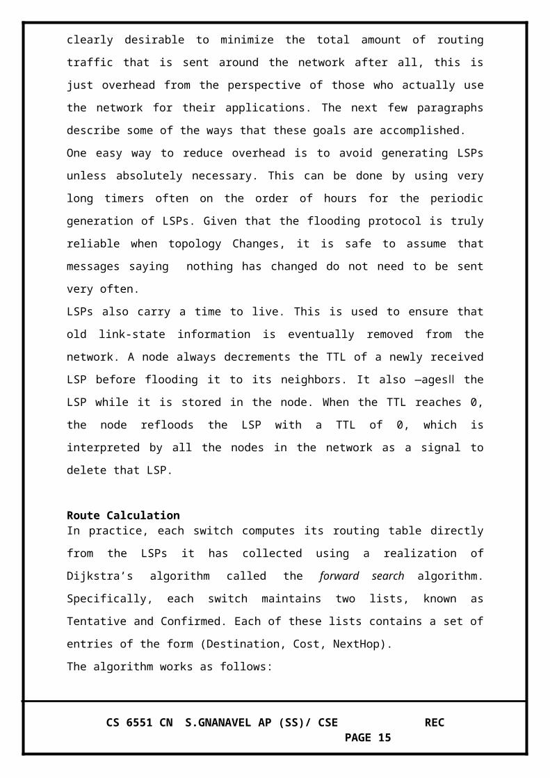
return to step 2. Link-state routing: an example network.
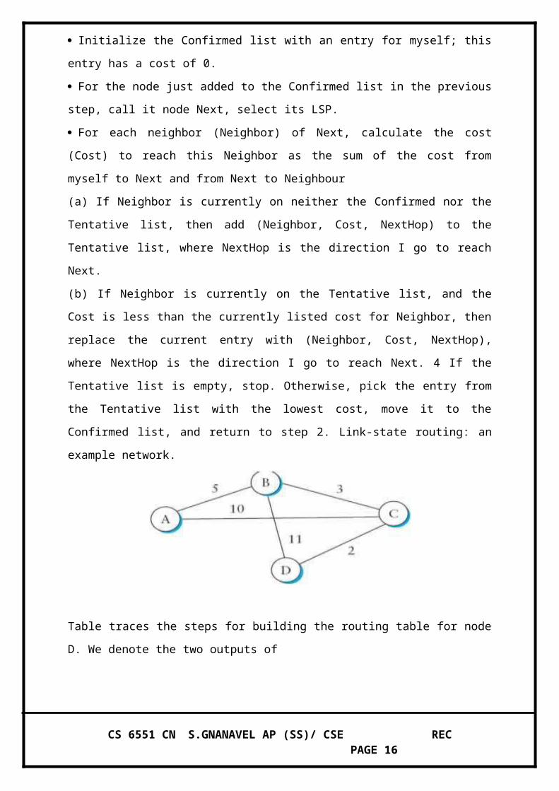
Table traces the steps for building the routing table for node D. We denote the two outputs of
D by using the names of the nodes to which they connect, B and C. Note the way the
algorithm seems to head off on false leads (like the 11-unit cost path to B that was the first
addition to the Tentative list) but ends up with the least-cost paths to all nodes.
CS 6551 CN S.GNANAVEL AP (SS)/ CSE REC PAGE 11
The Open Shortest Path First Protocol (OSPF)
One of the most widely used link-state routing protocols is OSPF. The first word, Open,refers to the fact that it is an open, non-proprietary standard, created under the auspices of the IETF. The ―SPF part comes from an alternative name for link state routing.
OSPF adds quite a number of features to the basic link-state algorithm described above, including the following:
Authentication of routing messages: This is a nice feature, since it is all too common for some misconfigured host to decide that it can reach every host in the universe at a cost of 0. When the host advertises this fact, every router in the surrounding neighbourhood updates
its forwarding tables to point to that host, and said host receives a vast amount of data that, in reality, it has no idea what to do with. This is not a strong enough form of authentication to prevent dedicated malicious users, but it alleviates many problems caused by misconfiguration.
Additional hierarchy: Hierarchy is one of the fundamental tools used to make systems more scalable. OSPF introduces another layer of hierarchy into routing by allowing a domain to be partitioned into areas. This means that a router within a domain does not necessarily
need to know how to reach every network within that domain— it may be sufficient for it to know only how to get to the right area. Thus, there is a reduction in the amount of information that must be transmitted to and stored in each node.
Load balancing: OSPF allows multiple routes to the same place to be assigned the same cost and will cause traffic to be distributed evenly over those route.
CS 6551 CN S.GNANAVEL AP (SS)/ CSE REC PAGE 12
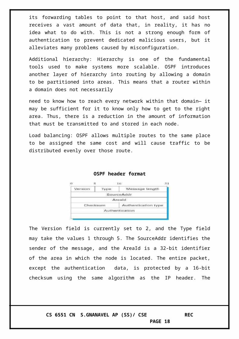
OSPF header format
The Version field is currently set to 2, and the Type field may take the values 1 through 5.
The SourceAddr identifies the sender of the message, and the AreaId is a 32-bit identifier of
the area in which the node is located. The entire packet, except the authentication data, is
protected by a 16-bit checksum using the same algorithm as the IP header. The
Authentication type is 0 if no authentication is used; otherwise it may be 1, implying a simple
password is used, or 2, which indicates that a cryptographic authentication checksum. In the
latter cases the Authentication field carries the password or cryptographic checksum.
Of the five OSPF message types, type 1 is the ―hello message, which a router sends to its
peers to notify them that it is still alive and connected as described above. The remaining
types are used to request, send, and acknowledge the receipt of linkstate messages. The basic
building block of link-state messages in OSPF is known as the link-state advertisement
(LSA).
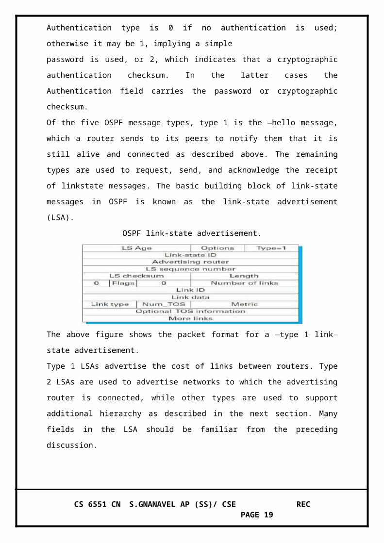
OSPF link-state advertisement.
The above figure shows the packet format for a ―type 1 link-state advertisement.
Type 1 LSAs advertise the cost of links between routers. Type 2 LSAs are used to advertise
networks to which the advertising router is connected, while other types are used to support
additional hierarchy as described in the next section. Many fields in the LSA should be
familiar from the preceding discussion.
The LS Age is the equivalent of a time to live, except that it counts up and the LSA expires
when the age reaches a defined maximum value. The Type field tells us that this is a type 1
LSA. In a type 1 LSA, the Link-state ID and the Advertising router field are identical.
CS 6551 CN S.GNANAVEL AP (SS)/ CSE REC PAGE 13
Each carries a 32-bit identifier for the router that created this LSA. While a number of
assignment strategies may be used to assign this ID, it is essential that it be unique in the
routing domain and that a given router consistently uses the same router ID. One way to pick
a router ID that meets these requirements would be to pick the lowest IP address among all
the IP addresses assigned to that router. (Recall that a router may Have a different IP address
on each of its interfaces.).The LS sequence number is used exactly as described above, to
detect old or duplicate LSAs. The LS checksum it is of course used to Verify that data has not
been corrupted. It covers all fields in the packet except LS Age, so that it is not necessary to
recompute a checksum every time LS Age is incremented. Length is the length in bytes of the
Now we get to the actual link-state information.
This is made a little complicated by the presence of TOS (type of service) information.
Ignoring that for a moment, each link in the LSA is represented by a Link ID, some Link
Data, and a metric. The first two of these fields identify the link; a common way to do this
would be to use the router ID of the router at the far end of the link as the Link ID, and then
use the Link Data to disambiguate among multiple parallel links if necessary. The metric is of
course the cost of the link. Type tells us something about the link, for example, if it is a point-
to-point link. The TOS information is present to allow OSPF to choose different routes for IP
packets based on the value in their TOS field. Instead of assigning a single metric to a link, it
is possible to assign different metrics depending on the TOS value of the data.
Metrics
The preceding discussion assumes that link costs, or metrics, are known when we execute the routing
algorithm. In this section, we look at some ways to calculate link costs that have proven effective in
practice. One example that we have seen already, which is quite reasonable and very simple, is to
assign a cost of 1 to all links—the least-cost route will then be the one with the fewest hops. Such an
approach has several drawbacks, however. First, it does not distinguish between links on a latency
basis.
Thus, a satellite link with 250-ms latency looks just as attractive to the routing protocol as a terrestrial
link with 1-ms latency. Second, it does not distinguish between routes on a capacity basis, making a
9.6-kbps link look just as good as a 45-Mbps link. Finally, it does not distinguish between links based
on their current load, making it impossible to route around overloaded links. It turns out that this last
problem is the hardest because you are trying to capture the complex and dynamic characteristics of a
link in a single scalar cost.
CS 6551 CN S.GNANAVEL AP (SS)/ CSE REC PAGE 14
The ARPANET was the testing ground for a number of different approaches to link-cost calculation.
(It was also the place where the superior stability of link-state over distance-vector routing was
demonstrated;
the original mechanism used distance vector while the later version used link state.) The following
discussion traces the evolution of the ARPANET routing metric and, in so doing, explores the subtle
aspects of the problem.
The original ARPANET routing metric measured the number of packets that were queued waiting to
be transmitted on each link, meaning that a link with 10 packets queued waiting to be transmitted was
assigned a larger cost weight than a link with 5 packets queued for transmission. Using queue length
as a routing metric did not work well, however, since queue length is an artificial measure of load it
moves packets toward the shortest queue rather than toward the destination, a situation all too familiar
to those of us who hop from line to line at the grocery store. Stated more precisely, the original
ARPANET routing mechanism suffered from the fact that it did not take either the bandwidth or the
latency of the link into consideration.
A second version of the ARPANET routing algorithm, sometimes called the new routing mechanism,
took both link bandwidth and latency into consideration and used delay, rather than just queue length,
as a measure of load. This was done as follows. First, each incoming packet was timestamped with its
time of arrival at the router (ArrivalTime); its departure time from the router (DepartTime) was also
recorded. Second, when the link-level ACK was received from the other side, the node computed the
delay for that packet as
Delay = (DepartTime−ArrivalTime)+TransmissionTime+Latency
where TransmissionTime and Latency were statically defined for the link and captured the link’s
bandwidth and latency, respectively. Notice that in this case, DepartTime − ArrivalTime represents
the amount of time the packet was delayed (queued) in the node due to load.
If the ACK did not arrive, but instead the packet timed out, then DepartTime was reset to the time the
packet was retransmitted. In this case, DepartTime – ArrivalTime captures the reliability of the link—
the more frequent the retransmission of packets, the less reliable the link, and the more we want to
avoid it. Finally, the weight assigned to each link was derived from the average delay experienced by
the packets recently sent over that link. Although an improvement over the original mechanism, this
approach also had a lot of problems. Under light load, it worked reasonably well, since the two static
factors of delay dominated the cost.
Under heavy load, however, a congested link would start to advertise a very high cost. This caused all
the traffic to move off that link, leaving it idle, so then it would advertise a low cost, thereby attracting
back all the traffic, and so on. The effect of this instability was that, under heavy load, many links
CS 6551 CN S.GNANAVEL AP (SS)/ CSE REC PAGE 15
would in fact spend a great deal of time being idle, which is the last thing you want under heavy load.
Another problem was that the range of link values was much too large. For example, a heavily loaded
9.6-kbps link could look 127 times more costly than a lightly loaded 56-kbps link.
This means that the routing algorithm would choose a path with 126 hops of lightly loaded 56-kbps
links in preference to a 1-hop 9.6-kbps path. While shedding some traffic from an overloaded line is a
good idea, making it look so unattractive that it loses all its traffic is excessive. Using 126 hops when
1 hop will do is in general a bad use of network resources.
Also, satellite links were unduly penalized, so that an idle 56-kbps satellite link looked considerably
more costly than an idle 9.6-kbps terrestrial link, even though the former would give better
performance for high-bandwidth applications.
A third approach, called the “revised ARPANET routing metric,” addressed these problems. The
major changes were to compress the dynamic range of the metric considerably, to account for the link
type, and to smooth the variation of the metric with time.
The smoothing was achieved by several mechanisms. First, the delay measurement was transformed
to a link utilization, and this number was
averaged with the last reported utilization to suppress sudden changes.
Second, there was a hard limit on how much the metric could change from one measurement cycle to
the next. By smoothing the changes in the cost, the likelihood that all nodes would abandon a route at
once is greatly reduced.
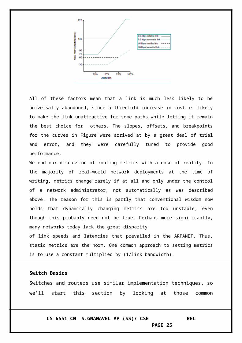
The compression of the dynamic range was achieved by feeding the measured utilization, the link
type, and the link speed into a function that is shown graphically in Figure .
Observe the following: n A highly loaded link never shows a cost of more than three times its cost
when idle.
n The most expensive link is only seven times the cost of the least expensive.
n A high-speed satellite link is more attractive than a low-speed terrestrial link.
n Cost is a function of link utilization only at moderate to high loads.
CS 6551 CN S.GNANAVEL AP (SS)/ CSE REC PAGE 16
All of these factors mean that a link is much less likely to be universally abandoned, since a threefold
increase in cost is likely to make the link unattractive for some paths while letting it remain the best
choice for others. The slopes, offsets, and breakpoints for the curves in Figure were arrived at by a
great deal of trial and error, and they were carefully tuned to provide good performance.
We end our discussion of routing metrics with a dose of reality. In the majority of real-world network
deployments at the time of writing, metrics change rarely if at all and only under the control of a
network administrator, not automatically as was described above. The reason for this is partly that
conventional wisdom now holds that dynamically changing metrics are too unstable, even though this
probably need not be true. Perhaps more significantly, many networks today lack the great disparity
of link speeds and latencies that prevailed in the ARPANET. Thus, static metrics are the norm. One
common approach to setting metrics is to use a constant multiplied by (1/link bandwidth).
Switch Basics
Switches and routers use similar implementation techniques, so we’ll start this section by
looking at those common techniques, then move on to look at the specific issues affecting
router implementation in this Section For most of this section, we’ll use the word switch to
cover both types of devices, since their internal designs are so similar (and it’stedious to say
“switch or router” all the time).
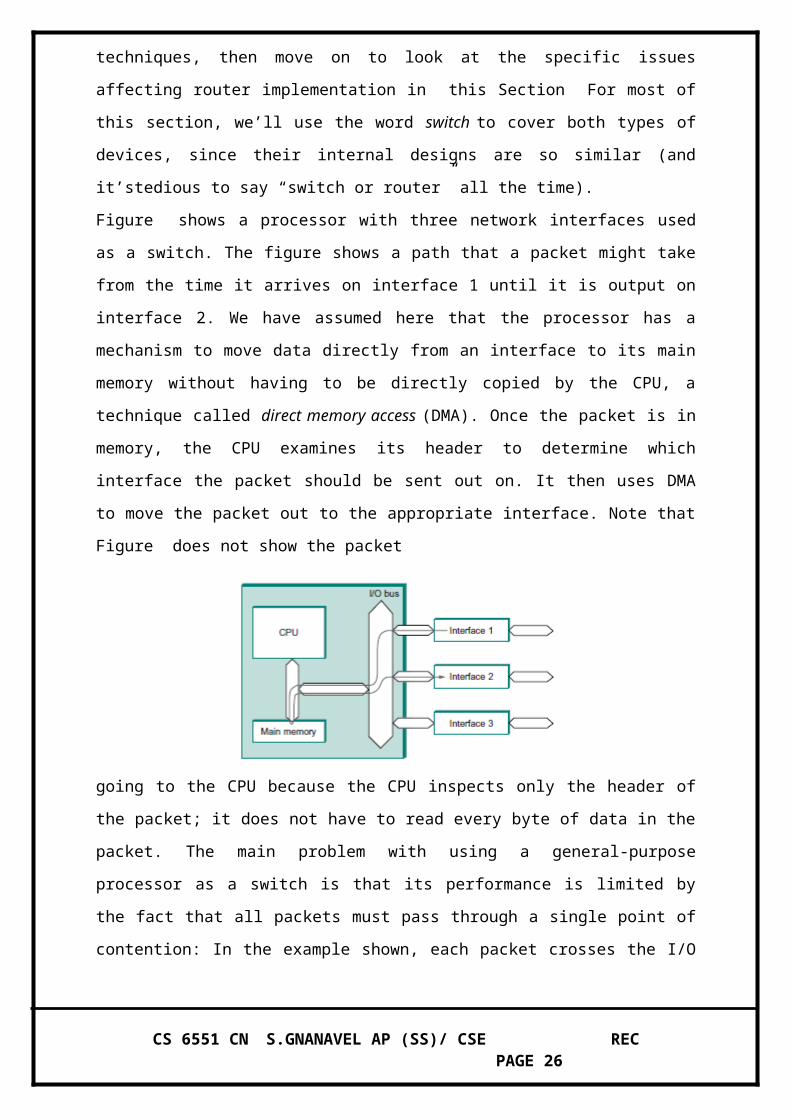
Figure shows a processor with three network interfaces used as a switch. The figure shows a
path that a packet might take from the time it arrives on interface 1 until it is output on
interface 2. We have assumed here that the processor has a mechanism to move data directly
from an interface to its main memory without having to be directly copied by the CPU, a
technique called direct memory access (DMA). Once the packet is in memory, the CPU
examines its header to determine which interface the packet should be sent out on. It then
uses DMA to move the packet out to the appropriate interface. Note that Figure does not
show the packet
going to the CPU because the CPU inspects only the header of the packet; it does not have to
read every byte of data in the packet. The main problem with using a general-purpose
CS 6551 CN S.GNANAVEL AP (SS)/ CSE REC PAGE 17
processor as a switch is that its performance is limited by the fact that all packets must pass
through a single point of contention: In the example shown, each packet crosses the I/O bus
twice and is written to and read from main memory once. The upper bound on aggregate
throughput of such a device (the total sustainable data rate summed over all inputs) is, thus,
either half the main memory bandwidth or half the I/O bus bandwidth, whichever is less.
(Usually, it’s the I/O bus bandwidth.) For example, a machine with a 133-MHz, 64-bit-wide
I/O bus can transmit data at a peak rate of a little over 8 Gbps. Since forwarding a packet
involves crossing the bus twice, the actual limit is 4 Gbps—enough to build a switch with a
fair number of 100-Mbps Ethernet ports, for example, but hardly enough for a high-end
router in the core of the Internet.
Moreover, this upper bound also assumes that moving data is the only problem a fair
approximation for long packets but a bad one when packets are short. In the latter case, the
cost of processing each packet parsing its header and deciding which output link to transmit it
on is likely to dominate. Suppose, for example, that a processor can perform all the necessary
processing to switch 2 million packets each second. This is sometimes called the packet per
second (pps) rate. (This number is representative of what is achievable on an inexpensive
PC.) If the average packet is short, say, 64 bytes, this would imply
Throughput = pps×(BitsPerPacket)
= 2×106 ×64×8
= 1024×106
that is, a throughput of about 1 Gbps—substantially below the range that users are demanding
from their networks today. Bear in mind that this 1 Gbps would be shared by all users
connected to the switch, just as the bandwidth of a single (unswitched) Ethernet segment is
shared among all users connected to the shared medium. Thus, for example, a 20-port switch
with this aggregate throughput would only be able to cope with an average data rate of about
50 Mbps on each port.
To address this problem, hardware designers have come up with a large array of switch
designs that reduce the amount of contention and provide high aggregate throughput. Note
that some contention is unavoidable: If every input has data to send to a single output, then
they cannot all send it at once. However, if data destined for different outputs is arriving at
different inputs,then a well-designed switch will be able to move data from inputs to outputs
in parallel, thus increasing the aggregate throughput.
CS 6551 CN S.GNANAVEL AP (SS)/ CSE REC PAGE 18
THE GLOBAL INTERNETAt this point, we have seen how to connect a heterogeneous collection of networks to create
an internetwork and how to use the simple hierarchy of the IP address to make routing in an
internet somewhat scalable. We say “somewhat” scalable because, even though each router
does not need to know about all the hosts connected to the internet, it does, in the model
described so far, need to know about all the networks connected to the internet. Today’s
Internet has hundreds of thousands of networks connected to it (or more, depending on how
you count). Routing protocols such as those we have just discussed do not scale to those
kinds of numbers.
This section looks at a variety of techniques that greatly improve scalability and that have
enabled the Internet to grow as far as it has. Before getting to these techniques, we need to
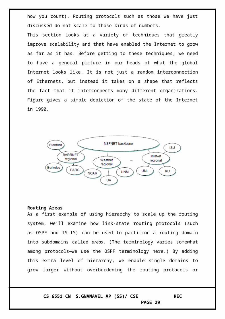
have a general picture in our heads of what the global Internet looks like. It is not just a
random interconnection of Ethernets, but instead it takes on a shape that reflects the fact that
it interconnects many different organizations. Figure gives a simple depiction of the state of
the Internet in 1990.
Routing AreasAs a first example of using hierarchy to scale up the routing system, we’ll examine how link-
state routing protocols (such as OSPF and IS-IS) can be used to partition a routing domain
into subdomains called areas. (The terminology varies somewhat among protocols—we use
the OSPF terminology here.) By adding this extra level of hierarchy, we enable single
domains to grow larger without overburdening the routing protocols or resorting to the more
complex interdomain routing protocols described below.
An area is a set of routers that are administratively configured to exchange link-state
information with each other. There is one special area—the backbone area, also known as
CS 6551 CN S.GNANAVEL AP (SS)/ CSE REC PAGE 19

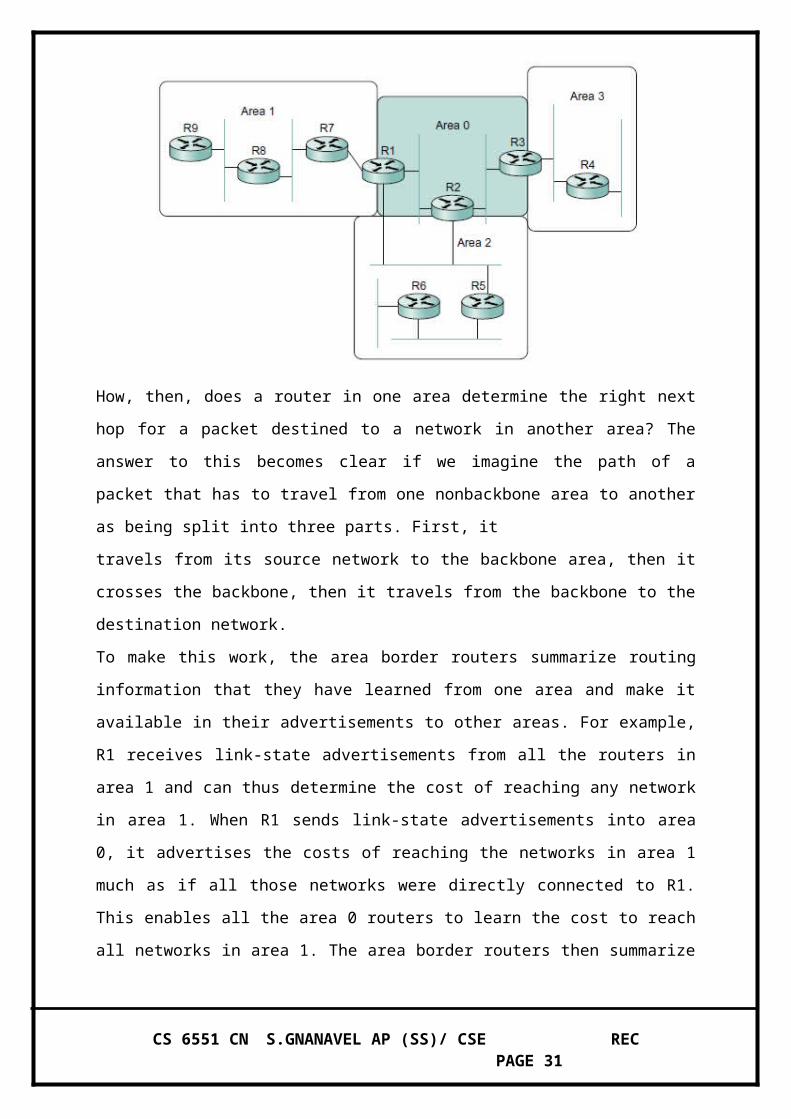
area 0. An example of a routing domain divided into areas is shown in Figure . Routers R1,
R2, and R3 are members of the backbone area. They are also members of at least one
nonbackbone area; R1 is actually a member of both area 1 and area 2.
A router that is a member of both the backbone area and a nonbackbone area is an area border
router (ABR). Note that these are distinct from the routers that are at the edge of an AS,
which are referred to as AS border routers for clarity Routing within a single area is exactly .
All the routers in the area send link-state advertisements to each other and thus develop a
complete, consistent map of the area. However, the link-state advertisements of routers that
are not area border routers do not leave the area in which they originated. This has the effect
of making the flooding and route calculation processes considerably more scalable.
For example, router R4 in area 3 will never see a link-state advertisement from router R8 in
area 1. As a consequence, it will know nothing about the detailed topology of areas other than
its own.
How, then, does a router in one area determine the right next hop for a packet destined to a
network in another area? The answer to this becomes clear if we imagine the path of a packet
that has to travel from one nonbackbone area to another as being split into three parts. First, it
travels from its source network to the backbone area, then it crosses the backbone, then it
travels from the backbone to the destination network.
To make this work, the area border routers summarize routing information that they have
learned from one area and make it available in their advertisements to other areas. For
example, R1 receives link-state advertisements from all the routers in area 1 and can thus
determine the cost of reaching any network in area 1. When R1 sends link-state
advertisements into area 0, it advertises the costs of reaching the networks in area 1 much as
CS 6551 CN S.GNANAVEL AP (SS)/ CSE REC PAGE 20
if all those networks were directly connected to R1. This enables all the area 0 routers to learn
the cost to reach all networks in area 1. The area border routers then summarize this
information and advertise it into the nonbackbone areas. Thus, all routers learn how to reach
all networks in the domain. Note that, in the case of area 2, there are two ABRs and that
routers in area 2 will thus have to make a choice as to which one they use to reach the
backbone. This is easy enough, since both R1 and R2 will be advertising costs to various
networks, so it will become clear which is the better choice as the routers in area 2 run their
shortest-path algorithm.
For example, it is pretty clear that R1 is going to be a better choice than R2 for destinations in
area 1.When dividing a domain into areas, the network administrator makes a tradeoff
between scalability and optimality of routing. The use of areas forces all packets traveling
from one area to another to go via the backbone area, even if a shorter path might have been
available. For example, even if R4 and R5 were directly connected, packets would not flow
between them because they are in different nonbackbone areas. It turns out that the need for
scalability is often more important than the need to use the absolute shortest path.
Finally, we note that there is a trick by which network administrators can more flexibly
decide which routers go in area 0. This trick uses the idea of a virtual link between routers.
Such a virtual link is obtained by configuring a router that is not directly connected to area 0
to exchange backbone routing information with a router that is. For example, a virtual link
could be configured from R8 to R1, thus making R8 part of the backbone. R8 would now
participate in link-state advertisement flooding with the other routers in area 0. The cost of
the virtual link from R8 to R1 is determined by the exchange of routing information that takes
place in area 1. This technique can help to improve the optimality of routing.
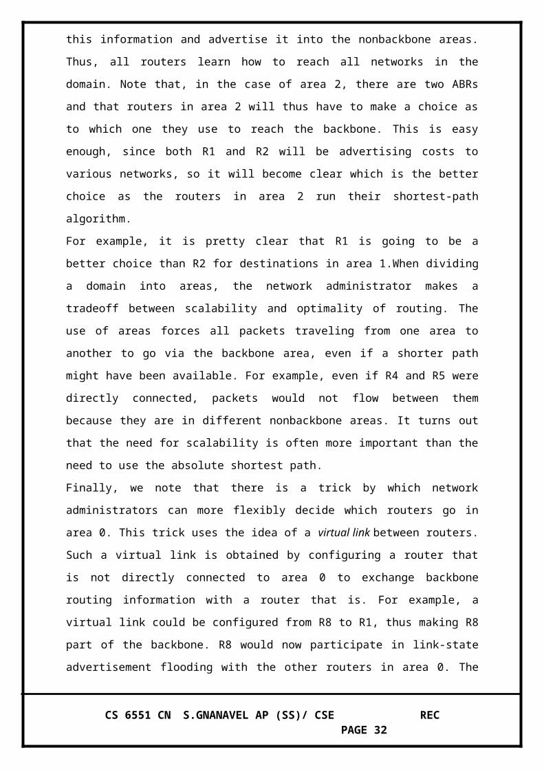
Network with two autonomous systems
CS 6551 CN S.GNANAVEL AP (SS)/ CSE REC PAGE 21
Interdomain Routing (BGP)
At the beginning of this chapter, we introduced the notion that the Inter- LAB 08 net is
organized as autonomous systems, each of which is under the BGP control of a single
administrative entity. A corporation’s complex internal network might be a single AS, as may
the network of a single Internet Service Provider (ISP). Figure shows a simple network with
two autonomous systems.
The basic idea behind autonomous systems is to provide an additional way to hierarchically
aggregate routing information in a large internet, thus improving scalability. We now divide
the routing problem into two parts: routing within a single autonomous system and routing
between autonomous systems. Since another name for autonomous systems in the Internet is
routing domains, we refer to the two parts of the routing problem as interdomain routing and
intradomain routing.
In addition to improving scalability, the AS model decouples the intradomain routing that
takes place in one AS from that taking place in another. Thus, each AS can run whatever
intradomain routing protocols it chooses. It can even use static routes or multiple protocols, if
desired. The interdomain routing problem is then one of having different ASs share
reachability information—descriptions of the set of IP addresses that can be reached via a
given AS—with each other.
Challenges in Interdomain Routing Perhaps the most important challenge of interdomain
routing today is the need for each AS to determine its own routing policies. A simple
example routing policy implemented at a particular AS might look like this: “Whenever
possible, I prefer to send traffic via AS X than via AS Y, but I’ll use AS Y if it is the only
path, and I never want to carry traffic from AS X to AS Y or vice versa.” Such a policy
would be typical when I have paid money to both AS X and AS Y to connect my AS to the
rest of the Internet, and AS X is my preferred provider of connectivity, with AS Y being the
fallback. Because I view both AS X and AS Y as providers (and presumably I paid them to
play this role), I don’t expect to help them out by carrying traffic between them across my
network (this is called transit traffic).
The more autonomous systems I connect to, the more complex policies I might have,
especially when you consider backbone providers, who may interconnect with dozens of
other providers and hundreds of customers and have different economic arrangements (which
affect routing policies) with each one.
A key design goal of interdomain routing is that policies like the example above, and much
more complex ones, should be supported by the interdomain routing system. To make the
CS 6551 CN S.GNANAVEL AP (SS)/ CSE REC PAGE 22
problem harder, I need to be able to implement such a policy without any help fromother
autonomous systems, and in the face of possible misconfiguration or malicious behaviour by
other autonomous systems. Furthermore, there is often a desire to keep the policies private,
because the entities that run the autonomous systems—mostly ISPs—are often in competition
with each other and don’t want their economic arrangements made public.
There have been two major interdomain routing protocols in the history of the Internet. The
first was the Exterior Gateway Protocol (EGP), which had a number of limitations, perhaps
the most severe of which was that it constrained the topology of the Internet rather
significantly.
EGP was designed when the Internet had a treelike topology, such as that illustrated in Figure
, and did not allow for the topology to become more general. Note that in this simple treelike
structure there is a single backbone, and autonomous systems are connected only as parents
and children and not as peers.
The replacement for EGP is the Border Gateway Protocol (BGP), which is in its fourth
version at the time of this writing (BGP-4). BGP is often regarded as one of the more
complex parts of the Internet. We’ll cover some of its high points here.
Unlike its predecessor EGP, BGP makes virtually no assumptions about how autonomous
systems are interconnected—they form an arbitrary graph. This model is clearly general
enough to accommodate non-treestructured internetworks, like the simplified picture of a
multi-provider Internet shown in Figure . (It turns out there is still some sort of structure to
the Internet, as we’ll see below, but it’s nothing like as simple as a tree, and BGP makes no
assumptions about such structure.)
simple picture in Figure today’s Internet consists of a richly interconnected set of networks,
mostly operated by private companies (ISPs) rather than governments. Many Internet Service
Providers (ISPs)
CS 6551 CN S.GNANAVEL AP (SS)/ CSE REC PAGE 23
exist mainly to provide service to “consumers” (i.e., individuals with computers in their
homes), while others offer something more like the old backbone service, interconnecting
other providers and sometimes larger corporations. Often, many providers arrange to
interconnect with each other at a single peering point.
To get a better sense of howwe might manage routing among this complex interconnection of
autonomous systems, we can start by defining a few terms. We define local traffic as traffic
that originates at or terminates on nodes within an AS, and transit traffic as traffic that passes
through an AS. We can classify autonomous systems into three broad types:
n Stub AS—an AS that has only a single connection to one other AS; such an AS will only
carry local traffic. The small corporation in Figure is an example of a stub AS.
n Multihomed AS—an AS that has connections to more than one other AS but that refuses to
carry transit traffic, such as the large corporation at the top of Figure n Transit AS—an AS
that has connections to more than one other AS and that is designed to carry both transit and
local traffic, such as the backbone providers in Figure .
Whereas the discussion of routing focused on finding optimal paths based on minimizing
some sort of link metric, the goals of interdomain routing are rather more complex. First, it is
necessary to find some path to the intended destination that is loop free. Second, paths must
be compliant with the policies of the various autonomous systems along the path—and, as we
have already seen, those policies might be almost arbitrarily complex. Thus, while
intradomain focuses on a welldefined problem of optimizing the scalar cost of the path,
interdomain focuses on finding a non-looping, policy-compliant path—a much more complex
optimization problem.
There are additional factors that make interdomain routing hard. The first is simply a matter
of scale. An Internet backbone router must be able to forward any packet destined anywhere
in the Internet. That means havinga routing table that will provide a match for any valid IP
address. While CIDR has helped to control the number of distinct prefixes that are carried
in the Internet’s backbone routing, there is inevitably a lot of routing information to pass
around—on the order of 300,000 prefixes at the time of writing.1
A further challenge in interdomain routing arises from the autonomous nature of the domains.
Note that each domain may run its own interior routing protocols and use any scheme it
chooses to assign metrics to paths. This means that it is impossible to calculate meaningful
path costs for a path that crosses multiple autonomous systems. A cost of 1000 across one
provider might imply a great path, but it might mean an unacceptably bad one from another
provider. As a result, interdomain routing advertises only reachability. The concept of
reachability is basically a statement that “you can reach this network through this AS.” This
CS 6551 CN S.GNANAVEL AP (SS)/ CSE REC PAGE 24
means that for interdomain routing to pick an optimal path is essentially impossible.
The autonomous nature of interdomain raises issue of trust. Provider A might be unwilling to
believe certain advertisements from provider B for fear that provider B will advertise
erroneous routing information. For example, trusting provider B when he advertises a great
route to anywhere in the Internet can be a disastrous choice if provider B turns out to have
made a mistake configuring his routers or to have insufficient capacity to carry the traffic.
The issue of trust is also related to the need to support complex policies as noted above. For
example, I might be willing to trust a particular provider only when he advertises
reachability to certain prefixes, and thus I would have a policy that says, “Use AS X to reach
only prefixes p and q, if and only if AS X advertises reachability to those prefixes.” Basics of
BGP Each AS has one or more border routers through which packets enter and leave the AS.
In our simple example in Figure , routers R2 and R4 would be border routers. (Over the
years, routers have sometimes also been known as gateways, hence the names of the
protocols BGP and EGP).
A border router is simply an IP router that is charged with the task of forwarding packets
between autonomous systems.
Each AS that participates in BGP must also have at least one BGP speaker, a router that
“speaks” BGP to other BGP speakers in other autonomous systems. It is common to find that
border routers are also BGP speakers, but that does not have to be the case.
BGP does not belong to either of the two main classes of routing protocols (distance-vector
and link-state protocols) Unlike these protocols, BGP advertises complete paths as an
enumerated list of autonomous systems to reach a particular network. It is sometimes called a
path-vector protocol for this reason. The advertisement of complete paths is necessary to
enable the sorts of policy decisions described above to be made in accordance with the
wishes of a particular AS. It also enables routing loops to be readily detected.
To see how this works, consider the very simple example network in Figure Assume that the
providers are transit networks, while the customer networks are stubs. A BGP speaker for the
AS of provider A (AS 2) would be able to advertise reachability information for each of the
network numbers assigned to customers P and Q. Thus, it would say, in effect, “The networks
128.96, 192.4.153, 192.4.32, and 192.4.3 can be reached directly from AS 2.” The backbone
network, on receiving this advertisement, can advertise, “The networks 128.96, 192.4.153,
192.4.32, and 192.4.3 can be reached along the path hAS 1, AS 2i.” Similarly, it could
advertise, “The networks 192.12.69, 192.4.54, and 192.4.23 can be reached along the path
hAS 1, AS 3i.” An important job of BGP is to prevent the establishment of looping paths.
CS 6551 CN S.GNANAVEL AP (SS)/ CSE REC PAGE 25
and AS 3, but the effect now is that the graph of autonomous systems has a loop in it.
Suppose AS 1 learns that it can reach network 128.96 through AS 2, so it advertises this fact
to AS 3, who in turn advertises it back to AS 2. In the absence of any loop prevention
mechanism, AS 2 could now decide that AS 3 was the preferred route for packets destined for
128.96. If AS 2 starts sending packets addressed to 128.96 to AS 3, AS 3 would send them to
AS 1; AS 1 would send them back to AS 2; and they would loop forever. This is prevented by
carrying the complete AS path in the routing messages. In this case, the advertisement for a
path to 128.96 received by AS 2 from AS 3 would contain an AS path of hAS 3, AS 1, AS 2,
AS 4i. AS 2 sees itself in this path, and thus concludes that this is not a useful path for it to
use.
In order for this loop prevention technique to work, the AS numbers carried in BGP clearly
need to be unique. For example, AS 2 can only recognize itself in the AS path in the above
example if no other AS identifies itself in the same way. AS numbers have until recently been
16-bit numbers, and they are assigned by a central authority to assure uniqueness.
BGP Updated packet format
CS 6551 CN S.GNANAVEL AP (SS)/ CSE REC PAGE 26
----------------------------------------------------------------------------------------------------------------
IP Version 6 (IPv6)
In many respects, the motivation for a new version of IP is simple: to deal with exhaustion of
the IP address space. CIDR helped considerably to contain the rate at which the Internet
address space is being consumed and also helped to control the growth of routing table
information needed in the Internet’s routers. However, there will come a point at which these
techniques are no longer adequate. In particular, it is virtually impossible to achieve 100%
address utilization efficiency, so the address space will be exhausted well before the 4
billionth host is connected to the Internet. Even if we were able to use all 4 billion addresses,
it’s not too hard to imagine ways that that number could be exhausted, now that IP addresses
are assigned not just to full-blowncomputers but also to mobile phones, televisions, and other
household appliances. All of these possibilities argue that a bigger address space than that
provided by 32 bits will eventually be needed.
Historical Perspective The IETF began looking at the problem of expanding the IP address
space in 1991, and several alternatives were proposed. Since the IP address is carried in the
header of every IP packet, increasing the size of the address dictates a change in the packet
header. This means a new version of the Internet Protocol and, as a consequence, a need for
new software for every host and router in the Internet. This is clearly not a trivial matter—it
is a major change that needs to be thought about very carefully. The effort to define a new
version of IP was known as IP Next Generation, or IPng. As the work progressed, an official
IP version number was assigned, so IPng is now known as IPv6. Note that the version of IP
discussed so far in this chapter is version 4 (IPv4). The apparent discontinuity in numbering
is the result of version number 5 being used for an experimental protocol some years ago.
CS 6551 CN S.GNANAVEL AP (SS)/ CSE REC PAGE 27
The significance of changing to a new version of IP caused a snowball effect. The general
feeling among network designers was that if you are going to make a change of this
magnitude you might as well fix as many other things in IP as possible at the same time.
Consequently, the IETF solicited white papers from anyone who cared to write one, asking
for input on the features that might be desired in a new version of IP. In addition to the need
to accommodate scalable routing and addressing, some of the other wish list items for IPng
included:
n Support for real-time services
n Security support
n Autoconfiguration (i.e., the ability of hosts to automatically configure themselves with such
information as their own IP address and domain name)
n Enhanced routing functionality, including support for mobile hosts It is interesting to note
that, while many of these features were absent from IPv4 at the time IPv6 was being
designed, support for all of them has made its way into IPv4 in recent years, often using
similar techniques in both protocols. It can be argued that the freedom to think of IPv6 as a
clean slate facilitated the design of new capabilities for IP that were then retrofitted into IPv4.
In addition to the wish list, one absolutely non-negotiable feature for IPng was that there must
be a transition plan to move from the current version of IP (version 4) to the new version.
With the Internet being so large and having no centralized control, it would be completely
impossible to have a “flag day” on which everyone shut down their hosts and routers and
installed a new version of IP. Thus, there will probably be a long transition period in which
some hosts and routers will run IPv4 only, some will run IPv4 and IPv6, and some will run
IPv6 only.
The IETF appointed a committee called the IPng Directorate to collect all the inputs on IPng
requirements and to evaluate proposals for a protocol to become IPng. Over the life of this
committee there were numerous proposals, some of which merged with other proposals, and
eventually one was chosen by theDirectorate to be the basis for IPng. That proposal was
called Simple Internet Protocol Plus (SIPP). SIPP originally called for a doubling of the IP
address size to 64 bits. When the Directorate selected SIPP, they stipulated several changes,
one of which was another doubling of the address to 128 bits (16 bytes). It was around this
time that version number 6 was assigned. The rest of this section describes some of the main
features of IPv6. At the time of this writing, most of the key specifications for IPv6 are
Proposed or Draft Standards in the IETF.
Addresses and Routing
CS 6551 CN S.GNANAVEL AP (SS)/ CSE REC PAGE 28
First and foremost, IPv6 provides a 128-bit address space, as opposed to the 32 bits of version
4. Thus, while version 4 can potentially address 4 billion nodes if address assignment
efficiency reaches 100%, IPv6 can address 3.4×1038 nodes, again assuming 100% efficiency.
As we have seen, though, 100% efficiency in address assignment is not likely. Some analysis
of other addressing schemes, such as those of the French and U.S. telephone networks, as
well as that of IPv4, have turned up some empirical numbers for address assignment
efficiency. Based on the most pessimistic estimates of efficiency drawn from this study, the
IPv6 address space is predicted to provide over 1500 addresses per square foot of the Earth’s
surface, which certainly seems like it should serve us well even when toasters on Venus have
IP addresses.
Address Space Allocation
Drawing on the effectiveness of CIDR in IPv4, IPv6 addresses are also classless, but the
address space is still subdivided in various ways based on the leading bits. Rather than
specifying different address classes, the leading bits specify different uses of the IPv6
address. The current assignment of prefixes is listed in Table .
This allocation of the address space warrants a little discussion. First, the entire functionality
of IPv4’s three main address classes (A, B, and C) is contained inside the “everything else”
range. Global Unicast Addresses, as we will see shortly, are a lot like classless IPv4
addresses, only much longer. These are the main ones of interest at this point, with over 99%
of the total IPv6 address space available to this important form of address. (At the time of
writing, IPv6 unicast addresses are being allocated from
Address prefix assignment for ipv6
the block that begins 001, with the remaining address space—about 87%—being reserved for
future use.)
The multicast address space is (obviously) for multicast, thereby serving the same role as
class D addresses in IPv4. Note that multicast addresses are easy to distinguish—they start
with a byte of all 1s.
CS 6551 CN S.GNANAVEL AP (SS)/ CSE REC PAGE 29
The idea behind link-local use addresses is to enable a host to construct an address that will
work on the network to which it is connected without being concerned about the global
uniqueness of the address. This may be useful for autoconfiguration, as we will see below.
Similarly, the site-local use addresses are intended to allow valid addresses to be constructed
ona site (e.g., a private corporate network) that is not connected to the larger Internet; again,
global uniqueness need not be an issue. Within the global unicast address space are some
important special types of addresses. A node may be assigned an IPv4-compatible IPv6
address by zero-extending a 32-bit IPv4 address to 128 bits. A node that is only capable of
understanding IPv4 can be assigned an IPv4-mapped IPv6 address by prefixing the 32-bit
IPv4 address with 2 bytes of all 1s and then zero-extending the result to 128 bits. These two
special address types have uses in the IPv4-to-IPv6 transition (see the sidebar on this topic).
Address Notation
Just as with IPv4, there is some special notation for writing down IPv6 addresses. The
standard representation is x:x:x:x:x:x:x:x, where each “x” is a hexadecimal representation of
a 16-bit piece of the address. An example would be
47CD:1234:4422:ACO2:0022:1234:A456:0124
Any IPv6 address can be written using this notation. Since there are a few special types of
IPv6 addresses, there are some special notations that may be helpful in certain circumstances.
For example, an address with a large number of contiguous 0s can be written more compactly
by omitting all the 0 fields. Thus,
47CD:0000:0000:0000:0000:0000:A456:0124
could be written
47CD::A456:0124
Clearly, this formof shorthand can only be used for one set of contiguous 0s in an address to
avoid ambiguity.
The two types of IPv6 addresses that contain an embedded IPv4 address have their own
special notation that makes extraction of the IPv4 address easier. For example, the IPv4-
mapped IPv6 address of a host whose IPv4 address was 128.96.33.81 could be written as
::FFFF:128.96.33.81
That is, the last 32 bits are written in IPv4 notation, rather than as a pair of hexadecimal
numbers separated by a colon.Note that the double colon at the front indicates the leading 0s.
Global Unicast Addresses
By far the most important sort of addressing that IPv6 must provide is plain old unicast
addressing. It must do this in a way that supports the rapid rate of addition of new hosts to the
Internet and that allows routing to be done in a scalable way as the number of physical
CS 6551 CN S.GNANAVEL AP (SS)/ CSE REC PAGE 30
networks in the Internet grows. Thus, at the heart of IPv6 is the unicast address allocation
plan that determines how unicast addresses will be assigned to service providers, autonomous
systems, networks, hosts, and routers. In fact, the address allocation plan that is proposed for
IPv6 unicast addresses is extremely similar to that being deployed with CIDR in IPv4.
To understand how it works and how it provides scalability, it is helpful to define some new
terms. We may think of a nontransit AS (i.e., a stub or multihomed AS) as a subscriber, and
we may think of a transit AS as a provider. Furthermore, we may subdivide providers into
direct and indirect. The former are directly connected to subscribers. The latter primarily
connect other providers, are not connected directly to subscribers, and are often known as
backbone networks. With this set of definitions, we can see that the Internet is not just an
arbitrarily interconnected set of autonomous systems; it has some intrinsic hierarchy. The
difficulty lies in making use of this hierarchywithout inventing mechanisms that fail when the
hierarchy is not strictly observed, as happened with EGP. For example, the distinction
between direct and indirect providers becomes blurred when a subscriber connects to a
backbone or when a direct provider starts connecting to many other providers.
As with CIDR, the goal of the IPv6 address allocation plan is to provide aggregation of
routing information to reduce the burden on intradomain routers. Again, the key idea is to use
an address prefix—a set of contiguous bits at the most significant end of the address—to
aggregate reachability information to a large number of networks and even to a large number
of autonomous systems. The main way to achieve this is to assign an address prefix to a
direct provider and then for that direct provider to assign longer prefixes that begin with that
prefix to its subscribers. for all of its subscribers. Of course, the drawback is that if a site
decides to change providers, it will need to obtain a new address prefix and renumber all the
nodes in the site. This could be a colossal undertaking, enough to dissuade most
people from ever changing providers. For this reason, there is ongoing research on other
addressing schemes, such as geographic addressing, in which a site’s address is a function of
its location rather than the provider to which it attaches. At present, however, provider-based
addressing is necessary to make routing work efficiently.
Note that while IPv6 address assignment is essentially equivalent to the way address
assignment has happened in IPv4 since the introduction of CIDR, IPv6 has the significant
advantage of not having a large installed base of assigned addresses to fit into its plans.
One question is whether it makes sense for hierarchical aggregation to take place at other
levels in the hierarchy. For example, should all providers obtain their address prefixes from
within a prefix allocated to the backbone to which they connect? Given that most providers
connect to multiple backbones, this probably doesn’t make sense. Also, since the number of
CS 6551 CN S.GNANAVEL AP (SS)/ CSE REC PAGE 31
providers is much smaller than the number of sites, the benefits of aggregating at this level
are much fewer. One place where aggregation may make sense is at the national or
continental level. Continental boundaries form natural divisions in the Internet topology. If all
addresses in Europe, for example, had a common prefix, then a great deal of aggregation
could be done, and most routers in other continents would only need one routing table entry
for all networks with the Europe prefix. Providers in Europe would all select their prefixes
such that they began with the European prefix.Using this scheme, an IPv6 address might look
like Figure 4.11. The RegistryID might be an identifier
assigned to a European address registry, with different IDs assigned to other continents or
countries. Note that prefixes would be of different lengths under this scenario. For example, a
provider with few customers could have a longer prefix (and thus less total address space
available) than one with many customers.
One tricky situation could occur when a subscriber is connected to more than one provider.
Which prefix should the subscriber use for his or her site? There is no perfect solution to the
problem. For example, suppose a subscriber is connected to two providers, X and Y. If the
subscriber takes his prefix from X, then Y has to advertise a prefix that has no relationship to
its other subscribers and that as a consequence cannot be aggregated. If the subscriber
numbers part of his AS with the prefix of X and part with the prefix of Y, he runs the risk of
having half his site become unreachable if the connection to one provider goes down. One
solution that works fairly well if X and Y have a lot of subscribers in common is for them to
have three prefixes between them: one for subscribers of X only, one for subscribers of Y
only, and one for the sites that are subscribers of both X and Y.
Packet Format
Despite the fact that IPv6 extends IPv4 in several ways, its header format is actually simpler.
This simplicity is due to a concerted effort to remove unnecessary functionality fromthe
protocol. Figure shows the result. As with many headers, this one starts with a Version field,
which is set to 6 for IPv6. The Version field is in the same place relative to the start of the
header as IPv4’s Version field so that header-processing software can immediately decide
which header format to look for. The TrafficClass and FlowLabel fields both relate to quality
of service issues.
CS 6551 CN S.GNANAVEL AP (SS)/ CSE REC PAGE 32
The PayloadLen field gives the length of the packet, excluding the IPv6 header, measured in
bytes. The NextHeader field cleverly replaces both the IP options and the Protocol field of
IPv4. If options are required, then
they are carried in one or more special headers following the IP header, and this is indicated
by the value of the NextHeader field. If there are no special headers, the NextHeader field is
the demux key identifying the higher-level protocol running over IP (e.g., TCP or UDP); that
is, it serves the same purpose as the IPv4 Protocol field. Also, fragmentation is now handled
as an optional header, which means that the fragmentationrelated fields of IPv4 are not
included in the IPv6 header. The HopLimit field is simply the TTL of IPv4, renamed to
reflect the way it is actually used.
Finally, the bulk of the header is taken up with the source and destination addresses, each of
which is 16 bytes (128 bits) long. Thus, the IPv6 header is always 40 bytes long. Considering
that IPv6 addresses are four times longer than those of IPv4, this compares quite well with
the IPv4 header, which is 20 bytes long in the absence of options.
The way that IPv6 handles options is quite an improvement over IPv4.In IPv4, if any options
were present, every router had to parse the entire options field to see if any of the options
were relevant. This is because the options were all buried at the end of the IP header, as an
unordered collection of htype, length, valuei tuples. In contrast, IPv6 treats options as
extension headers that must, if present, appear in a specific order. This means that each router
can quickly determine if any of the options are relevant to it; in most cases, they will not be.
Usually this can be determined by just looking at the NextHeader field. The end result is that
option processing is much more efficient in IPv6, which is an important factor in router
performance. In addition, the new formatting of options as extension headers means that they
CS 6551 CN S.GNANAVEL AP (SS)/ CSE REC PAGE 33
can be of arbitrary length, whereas in IPv4 they were limited to 44 bytes at most.We will see
how some of the options are used below.
Each option has its own type of extension header. The type of each extension header is
identified by the value of the NextHeader field in the header that precedes it, and each
extension header contains a NextHeader field to identify the header following it. The last
extension header will be followed by a transport-layer header (e.g., TCP) and in this case the
value of the NextHeader field is the same as the value of the Protocol field would be in an
IPv4 header. Thus, the NextHeader field does double duty; it may either identify the type of
extension header to follow, or, in the last extension header, it serves as a demux key to
identify the higher-layer protocol running over IPv6.
Consider the example of the fragmentation header, shown in Figure 4.13. This header
provides functionality similar to the fragmentationfields in the IPv4 .present if fragmentation
is necessary. Assuming it is the only extension header present, then the NextHeader field of
the IPv6 header would contain the value 44, which is the value assigned to indicate the
fragmentation header. The NextHeader field of the fragmentation header itself contains a
value describing the header that follows it. Again, assuming no other extension headers are
present, then the next header might be the TCP header, which results in NextHeader
containing the value 6, just as the Protocol field would in IPv4. If the fragmentation header
were followed by, say, an authentication header, then the fragmentation header’s NextHeader
field would contain the value 51.
Auto configuration
While the Internet’s growth has been impressive, one factor that has inhibited faster
acceptance of the technology is the fact that getting connected to the Internet has typically
required a fair amount of system administration expertise. In particular, every host that is
connected to the Internet needs to be configured with a certain minimum amount of
information,such as a valid IP address, a subnet mask for the link to which it attaches, and the
address of a name server. Thus, it has not been possible to unpack a new computer and
connect it to the Internet without some preconfiguration. One goal of IPv6, therefore, is to
provide support for autoconfiguration, sometimes referred to as plug-and-play operation.
CS 6551 CN S.GNANAVEL AP (SS)/ CSE REC PAGE 34
autoconfiguration is possible for IPv4, but it depends on the existence of a server that is
configured to hand out addresses and other configuration information to Dynamic Host
Configuration Protocol (DHCP) clients. The longer address format in IPv6 helps provide a
useful, new form of autoconfiguration called stateless autoconfiguration, which does not
require a server.
Recall that IPv6 unicast addresses are hierarchical, and that the least significant portion is the
interface ID. Thus, we can subdivide the autoconfiguration problem into two parts:
1. Obtain an interface ID that is unique on the link to which the host is attached.
2. Obtain the correct address prefix for this subnet.
The first part turns out to be rather easy, since every host on a link must have a unique link-
level address. For example, all hosts on an Ethernet have a unique 48-bit Ethernet address.
This can be turned into a valid link-local use address by adding the appropriate prefix from
Table
(1111 1110 10) followed by enough 0s to make up 128 bits. For some devices—for example,
printers or hosts on a small routerless network that do not connect to any other networks—
this address may be perfectly adequate.
Those devices that need a globally valid address depend on a router on the same link to
periodically advertise the appropriate prefix for the link. Clearly, this requires that the router
be configured with the correct address prefix, and that this prefix be chosen in such a way
that there is enough space at the end (e.g., 48 bits) to attach an appropriate link-level address.
The ability to embed link-level addresses as long as 48 bits into IPv6 addresses was one of
the reasons for choosing such a large address size. Not only does 128 bits allow the
embedding, but it leaves plenty of space for the multilevel hierarchy of addressing that we
discussedabove.
Advanced Routing Capabilities
Another of IPv6’s extension headers is the routing header. In the absence of this header,
routing for IPv6 differs very little from that of IPv4 under CIDR. The routing header contains
a list of IPv6 addresses that represent nodes or topological areas that the packet should visit
en route to its destination. A topological area may be, for example, a backbone provider’s
network. Specifying that packets must visit this network would be a way of implementing
provider selection on a packet-by-packet basis.
Thus, a host could say that it wants some packets to go through a provider that is cheap,
others through a provider that provides high reliability, and still others through a provider that
the host trusts to provide security.
CS 6551 CN S.GNANAVEL AP (SS)/ CSE REC PAGE 35
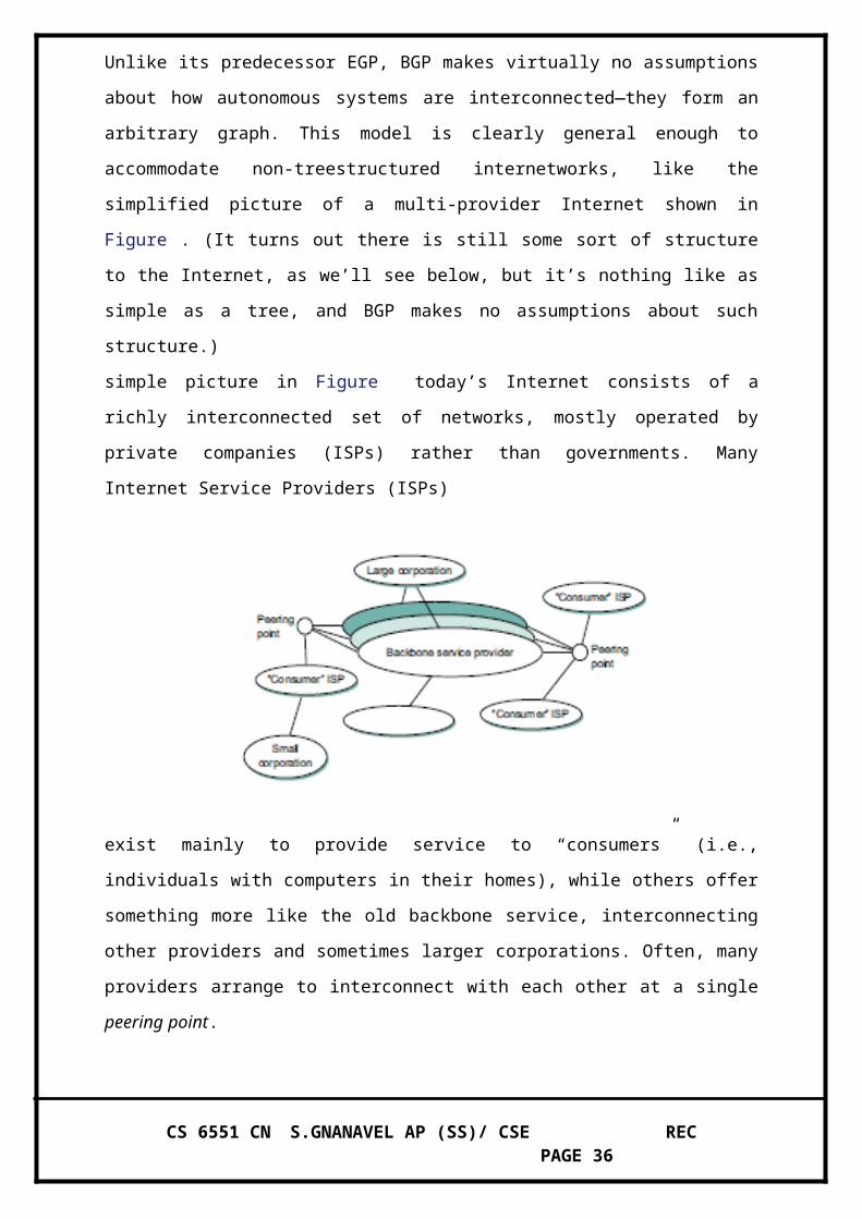
To provide the ability to specify topological entities rather than individual nodes, IPv6
defines an anycast address. An anycast address is assigned to a set of interfaces, and packets
sent to that address will go to the “nearest” of those interfaces, with nearest being determined
by the routing protocols. For example, all the routers of a backbone provider could be
assigned a single anycast address, which would be used in the routing header.
The anycast address and the routing header are also expected to be used to provide enhanced
routing support to mobile hosts. The detailed mechanisms for providing this support are still
being defined.
Other Features
As mentioned at the beginning of this section, the primary motivation behind the
development of IPv6 was to support the continued growth of the Internet. Once the IP header
had to be changed for the sake of the addresses, however, the door was open for a wide
variety of other changes, two of which we have just described—autoconfiguration and
source-directed routing. IPv6 includes several additional features, most of which are covered
elsewhere in this book.
Multicast Addresses
IP has a subrange of its address space reserved for multicast addresses. In IPv4, these
addresses are assigned in the class D address space, and IPv6 also has a portion of its address
space reserved for multicast group addresses. Some subranges of the multicast ranges are
reserved for intradomain multicast, so they can be reused independently by different domains.
There are thus 28 bits of possible multicast address in IPv4 when we ignore the prefix shared
by all multicast addresses. This presents a problem when attempting to take advantage of
hardware multicasting on a local area network (LAN). Let’s take the case of Ethernet.
Ethernet multicast addresses have only 23 bits when we ignore their shared prefix.
In other words, to take advantage of Ethernet multicasting, IP has to map28-bit IP multicast
addresses into 23-bit Ethernet multicast addresses. This is implemented by taking the low-
order 23 bits of any IP multicast address to use as its Ethernet multicast address and ignoring
the highorder 5 bits. Thus, 32 (25) IP addresses map into each one of the Ethernet addresses.
When a host on an Ethernet joins an IP multicast group, it configures its Ethernet interface to
receive any packets with the corresponding Ethernet multicast address. Unfortunately, this
causes the receiving host to receive not only the multicast traffic it desired but also traffic
sent to any of the other 31 IP multicast groups that map to the same Ethernet address, if they
are routed to that Ethernet. Therefore, IP at the receiving host must examine the IP header of
CS 6551 CN S.GNANAVEL AP (SS)/ CSE REC PAGE 36
any multicast packet to determine whether the packet really belongs to the desired group. In
summary, the mismatch of multicast address sizes means that multicast traffic may place a
burden on hosts that are not even interested in the group to which the traffic was sent.
Fortunately, in some switched networks (such as switched Ethernet) this problem can be
mitigated by schemes wherein the switches recognize unwanted packets and discard them.
One perplexing question is how senders and receivers learn which multicast addresses to use
in the first place. This is normally handled by out-of-band means, and there are some quite
sophisticated tools to enable group addresses to be advertised on the Internet
Multicast Routing
A router’s unicast forwarding tables indicate, for any IP address, which link to use to forward
the unicast packet. To support multicast, a router must additionally have multicast forwarding
tables that indicate, based on multicast address, which links—possibly more than one—to use
to forward the multicast packet (the router duplicates the packet if it is to be forwarded over
multiple links). Thus, where unicast forwarding tables collectively specify a set of paths,
multicast forwarding tables collectively specify a set of trees: multicast distribution trees.
Furthermore, to support Source-SpecificMulticast (and, it turns out, for some types of Any
Source Multicast), the multicast forwarding tables must indicate which links to use based on
the combination of multicast address and the (unicast) IP address of the source, again
specifying a set of trees.
Multicast routing is the process by which the multicast distribution trees are determined or,
more concretely, the process by which the multicast forwarding tables are built. As with
unicast routing, it is not enough that a multicast routing protocol “work”; it must also scale
reasonably well as the network grows, and it must accommodate the autonomy of different
routing domains.
DVMRP
Distance-vector routing, for unicast, can be extended to support multicast. The resulting
protocol is called Distance Vector Multicast Routing Protocol, or DVMRP. DVMRP was the
first multicast routing protocol to see widespread use.
Recall that, in the distance-vector algorithm, each router maintains a table of hDestination,
Cost, NextHopi tuples, and exchanges a list of hDestination, Costi pairs with its directly
connected neighbors. Extend- ing this algorithm to support multicast is a two-stage process.
First, we create a broadcast mechanism that allows a packet to be forwarded to all the
networks on the internet. Second, we need to refine this mechanism so that it prunes back
CS 6551 CN S.GNANAVEL AP (SS)/ CSE REC PAGE 37
networks that do not have hosts that belong to the multicast group. Consequently,DVMRP is
one of several multicast routing protocols described as flood-and-prune protocols.
Given a unicast routing table, each router knows that the current shortest path to a given
destination goes through NextHop. Thus, whenever it receives a multicast packet from source
S, the router forwards the packet on all outgoing links (except the one on which the packet
arrived) if and only if the packet arrived over the link that is on the shortest path to S (i.e., the
packet came from the NextHop associated with S in the routing table).
This strategy effectively floods packets outward from S but does not loop packets back
toward S.
There are two major shortcomings to this approach. The first is that it truly floods the
network; it has no provision for avoiding LANs that have no members in the multicast group.
We address this problem below. The second limitation is that a given packet will be
forwarded over a LAN by each of the routers connected to that LAN. This is due to the
forwarding strategy of flooding packets on all links other than the one on which the packet
arrived, without regard to whether or not those links are part of the shortest-path tree rooted
at the source.
The solution to this second limitation is to eliminate the duplicate broadcast packets that are
generated when more than one router is connected to a given LAN. One way to do this is to
designate one router as the parent router for each link, relative to the source, where only the
parent router is allowed to forward multicast packets from that source over the LAN. The
router that has the shortest path to source S is selected as the parent; a tie between two routers
would be broken according to which router has the smallest address. A given router can learn
if it is the parent for the LAN (again relative to each possible source) based upon the
distance-vector messages it exchanges with its neighbors.
Notice that this refinement requires that each router keep, for each source, a bit for each of its
incident links indicating whether or not it is the parent for that source/link pair. Keep in mind
that in an internet setting, a source is a network, not a host, since an internet router is only
interested in forwarding packets between networks. The resulting mechanism is sometimes
called Reverse Path Broadcast (RPB) or Reverse Path Forwarding (RPF). The path is reverse
because we are considering the shortest path toward the source when making our forwarding
decisions, as compared to unicast routing, which looks for the shortest path to a given
destination.
The RPB mechanism just described implements shortest-path broadcast. We now want to
prune the set of networks that receives each packet addressed to group G to exclude those
that have no hosts that are members of G. This can be accomplished in two stages. First, we
CS 6551 CN S.GNANAVEL AP (SS)/ CSE REC PAGE 38
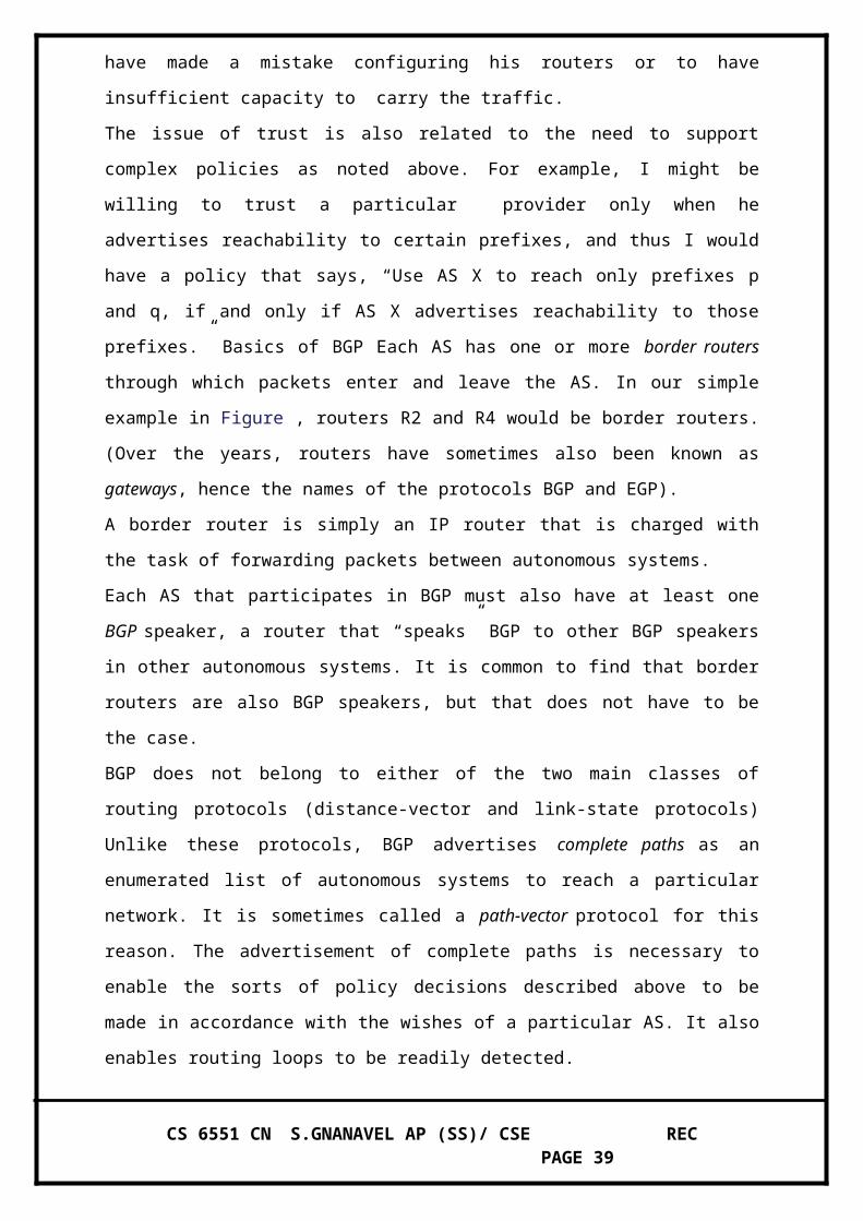
need to recognize when a leaf network has no group members. Determining that a network is
a leaf is easy—if the parent router as described above is the only router on the network, then
the network is a leaf. Determining if any group members reside on the network is
accomplished by having each host that is a member of group G periodically announce this
fact over the network, as described in our earlier description of link-state multicast.
The router then uses this information to decide whether or not to forward a multicast packet
addressed to G over this LAN.
The second stage is to propagate this “no members of G here” information up the shortest-
path tree. This is done by having the router augment the h Destination, Cost i pairs it sends to
its neighbors with the set of groups for which the leaf network is interested in receiving
multicast packets.
This information can then be propagated from router to router, so that for each of its links a
given router knows for what groups it should forward multicast packets.
Note that including all of this information in the routing update is a fairly expensive thing to
do. In practice, therefore, this information is exchanged only when some source starts sending
packets to that group.
In other words, the strategy is to use RPB, which adds a small amount of verhead to the basic
distance-vector algorithm, until a particular multicast address becomes active. At that time,
routers that are not interested in receiving packets addressed to that group speak up, and that
information is propagated to the other routers.
PIM-SM
Protocol Independent Multicast, or PIM, was developed in response to the scaling problems
of earlier multicast routing protocols. In particular, it was recognized that the existing
protocols did not scale well in environments where a relatively small proportion of routers
want to receive traffic for a certain group. For example, broadcasting traffic to all routers
until they explicitly ask to be removed from the distribution is not a good design choice if
most routers don’t want to receive the traffic in the first place. This situation is sufficiently
common that PIM divides the problem space into sparse mode and dense mode, where sparse
and dense refer to the proportion of routers that will want the multicast. PIM dense
mode (PIM-DM) uses a flood-and-prune algorithm like DVMRP and suffers from the same
scalability problem. PIM sparse mode (PIM-SM) has become the dominant multicast routing
protocol and is the focus of our discussion here. The “protocol independent” aspect of PIM,
by the way, refers to the fact that, unlike earlier protocols such as DVMRP, PIM does not
CS 6551 CN S.GNANAVEL AP (SS)/ CSE REC PAGE 39
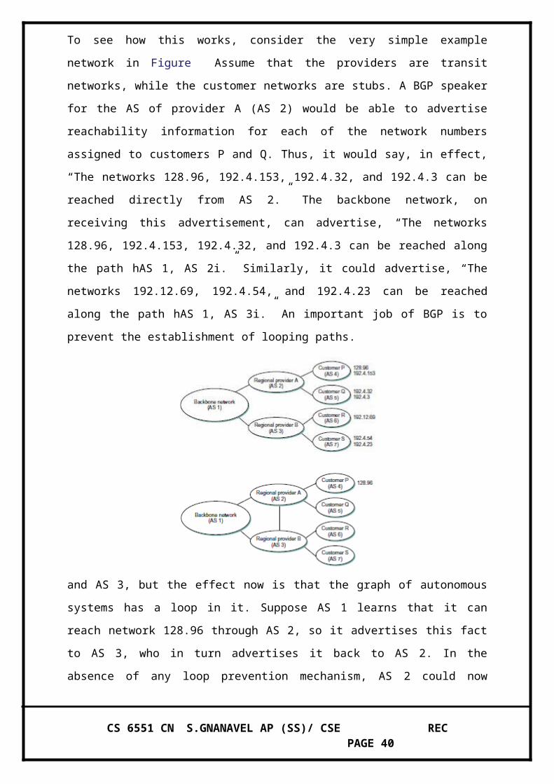
depend on any particular sort of unicast routing—it can be used with any unicast routing
protocol, as we will see below.
In PIM-SM, routers explicitly join the multicast distribution tree using PIM protocol
messages known as Join messages. Note the contrast to DVMRP’s approach of creating a
broadcast tree first and then pruning the uninterested routers. The question that arises is
where to send those Join messages because, after all, any host (and any number of hosts)
could send to the multicast group. To address this, PIM-SM assigns to each group a special
router known as the rendezvous point (RP). In general, a number of routers in a domain are
configured to be candidate RPs, and PIM-SM defines a set of procedures by which all the
routers in a domain can agree on the router to use as the RP for a given group. These
procedures are rather complex, as they must deal with a wide variety of scenarios, such as the
failure of a candidate RP and the partitioning of a domain into two separate networks due to a
number of link or node fail- ures. For the rest of this discussion,we assume that all routers in
a domain know the unicast IP address of the RP for a given group. A multicast forwarding
tree is built as a result of routers sending Join messages to the RP. PIM-SM allows two types
of trees to be constructed: a shared tree, which may be used by all senders, and a source-
specific tree, which may be used only by a specific sending host. The normal mode of
operation creates the shared tree first, followed by one or more source-specific trees if there is
enough traffic to warrant it. Because
CS 6551 CN S.GNANAVEL AP (SS)/ CSE REC PAGE 40
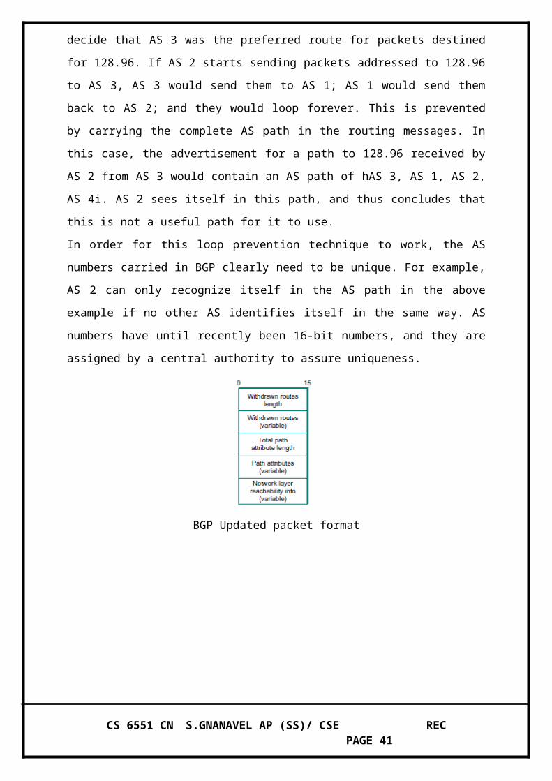
building trees installs state in the routers along the tree, it is important that the default is to
have only one tree for a group, not one for every sender to a group. When a router sends a
Join message toward the RP for a group G,it is sent using normal IP unicast transmission.
This is illustrated in Figure 4.14(a), inwhich router R4 is sending a Join to the rendezvous
point for some group. The initial Join message is “wildcarded”; that is, it applies to all
senders. A Join message clearly must pass through some sequence of routers before reaching
the RP (e.g., R2). Each router along the path looks at the Join and creates a forwarding table
entry for the shared tree, called a (*, G) entry (where * means “all senders”). To create the
forwarding table entry, it looks at the interface on which the Join arrived and marks that
interface as one on which it should forward data packets for this group. It then determines
which interface it will use to forward the Join toward the RP. This will be the only acceptable
interface for incoming packets sent to this group. It then forwards the Join toward the RP.
Eventually, the message arrives at the RP, completing the construction of the tree branch. The
shared tree thus constructed is shown as a solid line from the RP to R4 in Figure 4.14(a).
As more routers send Joins toward the RP, they cause new branches to be added to the tree,
as illustrated in Figure 4.14(b).Note that, in this case, the Join only needs to travel to R2,
which can add the new branch to the tree simply by adding a new outgoing interface to the
forwarding table entry created for this group. R2 need not forward the Join on to the RP.
Note also that the end result of this process is to build a tree whose root is the RP. At this
point, suppose a host wishes to send a message to the group. To do so, it constructs a packet
with the appropriate multicast group address as its destination and sends it to a router on its
local network known as the designated router (DR). Suppose the DR is R1 in Figure 4.14.
There is no state for this multicast group between R1 and the RP at this point, so instead of
simply forwarding the multicast packet, R1 tunnels it to the RP. That is, R1 encapsulates the
multicast packet inside a PIM Register message that it sends to the unicast IP address of the
RP. the RP receives the packet addressed to it, looks at the payload of the Register message,
and finds inside an IP packet addressed to the multicast address of this group. The RP, of
course, does know what to do with such a packet—it sends it out onto the shared tree of
which the RP is the root. In the example of Figure 4.14, this means that the RP sends the
packet on to R2, which is able to forward it on to R4 and R5. The complete delivery of a
packet from R1 to R4 and R5 is shown in Figure 4.15.We see the tunneled packet travel from
R1 to the RP with an extra IP header containing the unicast address of RP, and then the
multicast packet addressed to G making its way along the shared tree to R4 and R5.
At this point, we might be tempted to declare success, since all hosts can send to all receivers
this way. However, there is some bandwidth inefficiency and processing cost in the
CS 6551 CN S.GNANAVEL AP (SS)/ CSE REC PAGE 41
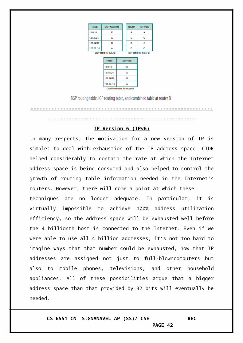
encapsulation and decapsulation of packets on the way to the RP, so the RP forces knowledge
about this
group into the intervening routers so tunneling can be avoided. It sends a Join message
toward the sending host (Figure 4.14(c)). As this Join travels toward the host, it causes the
routers along the path (R3) to learn about the group, so that it will be possible for the DR to
send the packet to the group as native (i.e., not tunneled) multicast packets.
An important detail to note at this stage is that the Join message sent by the RP to the sending
host is specific to that sender, whereas the previous ones sent by R4 and R5 applied to all
senders. Thus, the effect of the new Join is to create sender-specific state in the routers
between the identified source and the RP. This is referred to as (S, G) state, since it applies to
one sender to one group, and contrasts with the (*, G) state that was installed between the
receivers and the RP that applies to all senders.
Thus, in Figure 4.14(c), we see a source-specific route from R1 to the RP (indicated by the
dashed line) and a tree that is valid for all senders from the RP to the receivers (indicated by
the solid line). The next possible optimization is to replace the entire shared tree with a
source-specific tree. This is desirable because the path from sender to receiver via the RP
might be significantly longer than the shortest possible path. This again is likely to be
triggered by a high data rate being observed from some sender. In this case, the router at the
downstream end of the tree—say, R4 in our example—sends a source-specific Join toward
the source. As it follows the shortest path toward the source, the routers along the way create
(S, G) state for this tree, and the result is a tree that has its root at the source, rather than the
RP. Assuming both R4 and R5 made the witch to the source-specific tree, we would end up
with the tree shown in Figure 4.14(d). Note that this tree no longer involves the RP at all.We
CS 6551 CN S.GNANAVEL AP (SS)/ CSE REC PAGE 42
have removed the shared tree from this picture to simplify the diagram, but in reality all
routers with receivers for a group must stay on the shared tree in case new senders show up.
We can now see why PIM is protocol independent. All of its mechanisms for building and
maintaining trees take advantage of unicast routing without depending on any particular
unicast routing protocol.
The formation of trees is entirely determined by the paths that Join messagesfollow, which is
determined by the choice of shortest paths made by unicast routing. Thus, to be precise, PIM
is “unicast routing protocol independent,” as compared toDVMRP.Note that PIM is very
much bound up with the Internet Protocol—it is not protocol independent in terms of
network-layer protocols.
The design of PIM-SM again illustrates the challenges in building scalable networks and how
scalability is sometimes pitted against some sort of optimality. The shared tree is certainly
more scalable than a source specific tree, in the sense that it reduces the total state in routers
to be on the order of the number of groups rather than the number of senders times the
number of groups. However, the source-specific tree is likely to be necessary to achieve
efficient routing and effective use of link bandwidth.
CS 6551 CN S.GNANAVEL AP (SS)/ CSE REC PAGE 43