A simple and transferable all-atom/coarse-grained hybrid model to study membrane processes

Samuel Genheden*, Jonathan W. Essex

School of Chemistry, University of Southampton, Highfield, SO17 1BJ, Southampton, United Kingdom

*Correspondence to: s.genheden@soton.ac.uk

AbstractWe present an efficient all-atom/coarse-grained hybrid model and apply it to membrane processes. This model is an extension of the all-atom/ELBA model applied previously to processes in water. Here, we improve the efficiency of the model by implementing a multiple-timestep integrator that allows the atoms and the coarse-grained beads to be propagated at different timesteps. Furthermore, we fine-tune the interaction between the atoms and the coarse-grained beads by computing the potential of mean force of amino acid sidechain analogs along the membrane normal and comparing to atomistic simulations. The model was independently validated on the calculation of small-molecule partition coefficients. Finally, we apply the model to membrane peptides. We studied the tilt angle of the Walp23 and Kalp23 helices in two different model membranes and the stability of the glycophorin A dimer. The model is efficient, accurate and straightforward to use, as it does not require any extra interaction particles, layers of atomistic solvent molecules or tabulated potentials, thus offering a novel, simple approach to study membrane processes.

IntroductionThe cell membrane constitutes the barrier between the outside and the inside of the cell and therefore it is not surprising that a lot of interesting biology and chemistry take place within or near membranes. The membrane offers the first level of protection from foreign molecules, acts as a mediator in cell–cell communication, and nutrition essential for the cell as well as waste products need to be transported through it. Some of these processes are accomplished by passive diffusion and some other are carried out by membrane proteins.1,2 Because of their central role, membrane proteins are very common drug targets.3,4

Molecular dynamics is a computational tool commonly used to study membrane processes.5,6 Simulations offer a unique approach to study these systems at atomic resolution and have been used for instance to study permeability of small molecules,7,8,9,10,11 insertion of antimicrobial peptides,12 ion and water transport13,14 and self-assembly of membrane proteins.15,16 The simulations are almost always based on a force field that describes the molecules using classical mechanics, most commonly using analytical potentials, although tabulated potentials have been used.17 The most accurate force fields treat each atom individually with the drawback that they are computationally costly, thereby limiting the time and length scales that can be

1

modeled. As a consequence, coarse-graining has been used in which atoms are grouped into new, larger particles, offering the potential to model larger systems and longer scales by sacrificing accuracy.18,19 The least coarse-grained approach is united-atom force field that models all atoms, except non-polar hydrogen atoms that are merged with the carbon atom to which they are bound.20 A more invasive strategy is to group several heavy atoms (including hydrogen atoms) into bead particles. Examples of such force fields are the MARTINI,21,22,23 GROMOS24,25 and ELBA26,27 models. Such potentials are very popular as they can be used to model very large biomolecular systems that can be readily simulated for microseconds. Yet another coarse-grained approach is to neglect the particle description of the solvent altogether and treat it with continuum electrostatics. This approach is commonly used to model isotropic solvents such as water but has also been extended to the heterogeneous membrane environment.28,29,30

The sacrifice of accuracy in the CG models necessarily leads to some limitations. For instance, although the MARTINI model has parameterized force fields for proteins, making it possible to study large protein assemblies in model membranes, the proteins generally have to be restrained to the starting conformation.31,32 This makes it difficult to study conformational changes of membrane proteins. Furthermore, for small molecules, it is unrealistic to expect that a CG model could accurately describe the multitude of chemical entities available in nature without extensive parameterization. Whereas standardized and automatic procedures to derive all-atom force fields for small molecules exists,33,34,35 and are widely used, few such procedures has been proposed for CG potentials.36 Therefore, it is of interest to develop hybrid models that mix an all-atom description of the most interesting molecule, e.g. a protein or a small molecule, with a CG description of the solvent (water or lipid). This is akin to the much more mature quantum-mechanics/molecular-mechanics approach used to study processes where electronic degrees of freedom are important.37,38

Voth and co-workers developed a multiscale CG model39 (MS-CG) and later applied it to the study of the gramicidin A ion channel.17 The MS-CG model is attractive but requires an all-atom simulation to parameterize the tabulated potential used to model the interaction between the atoms and the CG beads.39 The GROMOS CG water model has been used to solvate proteins but it is recommended to include a layer of explicit water molecules between the CG water and the protein due to a lack of hydrogen bonding in the water model.40,41,42 This was also the approach used with the WatFour water model,43 making it difficult to extend to membrane proteins. The MARTINI model has been used in hybrid simulation as well,44,45 but it requires virtual particles to facilitate the interaction between the CG beads and the atoms. In a more recent attempt with the polarizable MARTINI water model,46 a dielectric-screening constant was introduced due to the lack of realistic electrostatics in MARTINI. A similar approach was used in the PACE model.47 The ELBA model on the other hand, was developed with the aim to model electrostatics explicitly using monopoles and dipoles.26,27 In the first parameterization, the lipids were based on ellipsoidal particles interacting through a Gay–Bern potential.26 Mixing with atomistic solutes were possible and this hybrid model was used successfully to study partition coefficients,48 permeability of small molecules49,50 and insertion of antimicrobials in model CG membranes.12 However, two scaling parameters were introduced to improve the interaction between the two resolutions, and only rigid atomistic solutes were inserted in the CG membrane.48 More recently, a new parameterization of ELBA has been presented that is a much simpler model based on spherical beads. Combined with an

2

atomistic description of solutes it was used to study the solvation of amino acid sidechain analogs and proteins in water as well as folding rates of small peptides.51 This all-atom/ELBA hybrid model was shown to be of similar accuracy as all-atom simulations but 3 to 6 times more computationally efficient.

In this paper we present an extension of the all-atom/ELBA hybrid model to the study of membrane systems. Although, we have used a hybrid approach previously to study such processes, it is important to re-evaluate it here due to the extensive reparameterization of the ELBA model. First, we improved the efficiency of the simulations by implementing a multiple-timestep integrator, ensuring that we can propagate the atomistic particles with a 2 to 4 fs timestep, and the CG beads with a 6 to 8 fs timestep. Second, we fine-tuned the interaction between the CG beads and the atoms by computing the potential of mean force (PMF) of amino acid sidechain analogs. Third and last, we validated the model by computing small-molecule partition coefficients and by studying the stability of transmembrane helices. The hybrid model is accurate, efficient and straightforward to use.

Figure 1. ELBA model of a water molecule and a DOPC lipid. The arrows indicate point dipoles and the plus and minus signs in the lipid head group indicate charges.

Methods

The ELBA potential. The ELBA (electrostatics based) potential has been described previously in the literature.27,52 Here we will only summarize it briefly. The ELBA water model is representing one real water molecule with a point dipole located in a van der Waals sphere as shown in Figure 1, i.e. a Stockmayer fluid. This water model has been validated on many physical properties53 and all-atom force fields can be mixed with it without any empirical scaling parameters.51 The ELBA model of a DOPC (1,2-dioleoyl-sn-glycero-3-phosphocholine) lipid molecule is also shown in Figure 1. All beads interacts through van der Waals interactions, and in addition the choline and phosphate beads are charged, and point dipoles are embedded in the glycerol and ester beads. This version of ELBA has been validated on several membrane properties,27,52 but has never been mixed with all-atom force fields. The pair-wise interactions are of a shifted-force kind with a 1.2 nm cut-off.27 Pair-wise

3

interactions between CG beads and atoms were also treated with such potentials and standard Lorentz-Berthelot mixing rules were applied as described previously.51

Here, we extended the ELBA force field with a model of a shorter, saturated lipid that can be used to represent DMPC (1,2-dimyristoyl-sn-glycero-3-phosphocholine). This model was created by removing the two terminal tail beads of the DOPC model and using the angle potential for saturated bonds on both chains. A pre-equilibrated bilayer structure was obtained in the following way: an all-atom configuration of a 72 or 128-lipid bilayer with 40 water molecules per lipid was created with the CHARMM Membrane Builder54 and mapped to the CG model using in-house scripts. This bilayer was then minimized for 100 steps with steepest descent, followed by 50 ps equilibration in the NVT ensemble, 500 ps equilibration in the NPT ensemble and a finally a 50 ns production run in the NPT ensemble. A 10 fs timestep was used, the temperature was kept at 303 K using a Langevin thermostat with a 10 ps time constant and the pressure was kept at 1 atm using a semi-isotropic weak-coupling algorithm with a 10 ps time constant,55 coupling the pressure of the membrane plane independently of the pressure along the bilayer normal. All simulations were performed with the Lammps software.56 This produced a bilayer that had an area per lipid of 0.69 nm2 and a volume per lipid of 1.166 nm3. The area and volume is slightly larger than the experimental values of DMPC 0.58–0.67 nm2 and 1.095–1.101 nm3, respectively6 but this is acceptable as the atomistic – coarse-grain mapping is not ideal due to the 3–1 mapping of the tail beads. Furthermore, as expected because of the inexact mapping, the bilayer thickness is only 3.1±0.5 nm compared to 3.4–3.6 nm as measured experimentally.6

The rRESPA integrator. We implemented an rRESPA (reversible reference system propagator algorithm) integrator57,58 in the Lammps software.55 The rRESPA framework in Lammps is that of a force-split rRESPA,57,59 and we extended this in the following way: all forces due to CG–CG interactions are updated at the outer rRESPA level, i.e., they are updated less often, and all other forces (CG–AA and AA–AA interactions as well as bonded forces) are updated in the inner level, i.e. they are updated more often. Accordingly, we will improve the computational efficiency by performing a majority of the force calculation less often, because the number of CG beads will exceed the number of atoms.

We validated the implementation by studying the energy conservation in an NVE simulation of benzene in a box of water. The benzene was parameterized with the general Amber force field33 (GAFF) and AM1-BCC charges60 using the Antechamber program,61 and solvated with 575 ELBA water molecules. The cut-off for AA–AA interactions was 1.2 nm and long-range electrostatics were treated with particle-particle particle-mesh Ewald summation (P3M).62 The system was equilibrated for 30 ps in the NVT ensemble using a weak-coupling thermostat at 298 K, followed by a NVE simulation for 1 ns. The inner rRESPA level was propagated with a 2 fs timestep and the outer level with a 4, 6, 8 or 10 fs timestep.

To further validate the integrator, we calculated the solvation free energy of benzene according to published protocols.51 In short, benzene was decoupled from the surroundings using an alchemical coupling parameter. The derivative of the energy with respect to this coupling parameter was then integrated numerically to obtain the negative of the solvation free energy. Standard errors were computed by performing two independent repeats.

4

Umbrella sampling simulations. The potential of mean force (PMF) of the amino acid sidechain analogs along the membrane normal was computed using umbrella sampling.63 All amino acids were modeled except His, Gly and Pro. The neutral form of Asp, Glu, Arg and Lys was used. The side-chains were truncated at the Cβ and capped with a hydrogen atom. The molecules were parameterized with GAFF33 and AM1-BCC charges59 using the Antechamber program,60 to be consistent with a previous study.51 The cut-off for AA–AA interactions were 1.2 nm and long-range electrostatics were treated with P3M.61

A single molecule was placed at a specific distance along the bilayer normal of a pre-equilibrated DOPC membrane (128 lipids and 4232 water molecules). The solutes were placed at distances of 0 to 3.0 nm from the bilayer center of mass in 0.1 nm increments. The interactions between the solute and the CG beads were then turned on smoothly during a 500 ps NPT simulation. The solute molecule was fixed at its initial position. The timestep for all forces was 1 fs to avoid numerical instabilities during this preparation phase. The temperature was kept at 298 K using a Langevin thermostat and the pressure was kept at 1 atm using a semi-isotropic weak-coupling algorithm both with a 10 ps time constant.55

This equilibrated system was then subjected to umbrella sampling.62 The solute was restrained at a specific distance along the bilayer normal with a harmonic spring with a force constant of 1046 kJ/mol/nm2. The system was simulated for 60 ns in the NPT ensemble with a 6 fs time step for the outer rRESPA level and 1–2 fs for the inner level at each restrained distance. The harmonic restraint was enforced in the inner rRESPA level. The instantaneous distance from the bilayer center was recorded every 0.9 ps. These distances were then used to compute the PMF with the weighted histogram analysis method (WHAM).64,65 The initial sixth of the simulation was discarded as equilibration and WHAM was applied to five equal, i.e. 10 ns, blocks of data to estimate the uncertainty.

Partition coefficients. The partition coefficient of eleven small molecules (glycerol, methanol, acetone, 1-butanol, benzylalcohol, aniline, 2-nitrotoluene, p-xylene, p-chlorocresol, 2,4,5-trichloroaniline, hexachlorobenzene) was estimated by computing the PMF along the membrane normal. The partition coefficients in DMPC have been determined by experiments.66,67,68,69,70 The procedure to calculate the PMF was identical to the procedure used for the amino acid sidechains, except that the PMF was computed in a DMPC membrane (72 lipids, 2376 waters) and only 30 ns sampling per window was used. As with the amino acid analogs, the small molecules were parameterized using GAFF and AM1-BCC charges. Four independent repeats were initiated by applying different starting velocities. The partition coefficients were estimated from the PMFs using the following equation.71,72,73

(1)

where G(z) is the PMF at depth z, wat(z) the water density at depth z, wat(z3.0) the water density in bulk, APL is the area pear lipid, Mlipids is the mass of the lipid and mu

is the atomic mass constant, and the integration is taken over the entire range for which the PMF was computed (z = 0 to 3.0 nm). This has been used previously to compute partition coefficients that are comparable to experiments.73

5

Kalp23 and Walp23 helices. The Kalp23 (GKKLALALALALALALALALKKA) and Walp23 (GWWLALALALALALALALALWWA) helices74,75 were built using UCSF Chimera76 and described with the Amber99SB force field.77 The terminal residue was uncharged but the Lys residues were kept charged. The mass of the hydrogen atoms was increased three-fold and the mass of the heavy atoms was decreased correspondingly through mass repartitioning to allow a longer timestep.78 The cut-off and treatment of long-range electrostatics were identical to the small-molecule simulations.

The helices were inserted into either a pre-equilibrated DOPC or DMPC membrane (128 lipids, ~ 4220 waters) according to the following procedure.79 The helices were placed 1 nm from the edge of membrane such that their principal axis was aligned with the membrane normal (see Figure S1). Then the system was simulated in the NPT ensemble for 1 ns. The timestep was 8 fs for the outer rRESPA level and 4 fs for the inner level. The temperature was kept at 300 K using a Langevin thermostat with a 10 ps time constant. The pressure along the membrane normal was kept at 1 atm using a weak-coupling algorithm with a relaxation time of 100 ps, whereas the pressure within the membrane plane was 1000 atm with a 100 ps relaxation time. The heavy atoms of the helix were restrained to the starting positions using a 10,460 kJ/mol/nm2 spring. The water, choline and terminal tail beads were restrained to their starting position along the membrane normal (but free to move in the membrane plane) with an identical force constant. These restraints together with the large pressure forces the membrane to envelope the helix. This high-pressure simulation was followed by a 2 ns simulation where the pressure within the membrane plane was 1 atm but with the same restraints on the CG beads and peptide atoms.

The prepared helix–membrane system was subjected to a 300 ns simulation in the NPT ensemble without restraints. Two independent repeats were initiated by assigning different starting velocities. The tilt angle, defined as the angle between the bilayer normal and the principal axis of the CA atoms in the helix, was measured with in-house scripts. The analysis was made on the last 200 ns of the simulations.

GpA dimer. The Glycophorin A (GpA) dimer80 was initialized from the fourth conformation of the 1AFO NMR structure81. Similarly to other studies,29,30,82 it was truncated to only include the transmembrane portion from Glu72 to Arg97. The terminal residues were uncharged. The dimer was described with the Amber99SB force field.77 It was inserted in a pre-equilibrated DMPC membrane (128 lipids, 4224 waters) using the same procedure as with the Kalp23 and Walp23 helices. The prepared system was subjected to 50 ns production simulation in the NPT ensemble without any restraints. Analyses were performed on the last 10 ns of the production simulation.

Results and discussion

6

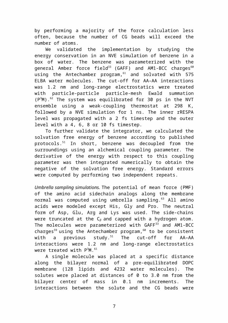
Figure 2. Total energy conservation in the simulation of atomistic benzene in coarse-grained water with different time steps. The different time steps refer to the outer

rRESPA loop; the inner time step was always 2 fs. For clarity, the time series for 6, 8 and 10 fs have been shifted up by 20, 40 and 60 kJ/mol, respectively.

The rRESPA integrator. The new integrator in LAMMPS was tested for energy conservation by NVE simulations of benzene in a box of ELBA waters. The conservation of the total energy is shown in Figure 2 for four different timesteps of the outer rRESPA level. The timestep for the inner level was always 2 fs. The ELBA water has been previously shown to be stable up to 10 fs53 and here we confirm that the hybrid simulation is also stable up to 10 fs. The fluctuations are always less than 0.01% of the average energy over the 1 ns simulation. In addition, the fluctuations in the potential and kinetic energy are always more than 10 times larger than the fluctuation in the total energy (not shown).83 Therefore, we can conclude that the force split is justifiable.

We also computed the solvation free energy of benzene in water and compared with the results obtained with the simple velocity-Verlet integrator (in which all forces are updated with a 2 fs timestep) and with experiment. The full results are listed in Supporting Information (Table S1). Using velocity-Verlet we computed a solvation free energy of –3.4 ± 0.6 kJ/mol, which accurately reproduces the experimental value of –3.8 kJ/mol.84 Irrespective of the timestep used with rRESPA, we obtained solvation free energies between –3.4 ± 0.8 and –5.1 ± 1.0 kJ/mol. Thus, we obtain comparable results with rRESPA because no difference was statistically significant (all p-values of a t-test are greater than 0.3). It should be noted that we did not attempt to improve the statistical uncertainty for either velocity-Verlet or rRESPA by running more independent repeats or longer simulations.

Lastly, we benchmarked the rRESPA integrator by performing 5 ps simulations of various systems; benzene in water, the BPTI protein85 in water, benzene in a DOPC membrane and the GpA protein in a DMPC membrane. Here we are not concerned with the speed or parallel performance of the Lammps software as such, but instead investigate how much computational gain we obtain with the new integrator. It should be noted that for the benzene in water system, the particle number is so low that Lammps does not scale up to more than 8 processors. Similarly, we would not expect Lammps to scale up to more than about 16 cores on the other three systems. In Figure 3, we plot the speed-up using rRESPA compared to the velocity-Verlet integrator on different numbers of processors (the two integrators always use the same number of processors). All benchmarks were performed on Intel 2.6 GHz processors. As seen

7

clearly in the plot, the efficiency of the rRESPA integrator is system dependent. For the benzene systems, the CG beads constitute 98 to 99% of the particles in the system and here we see that rRESPA can be 2 to 3 times faster than velocity-Verlet on 8 or 16 cores. For the BPTI protein, the proportion of CG beads is only 85% and it does not seem possible currently to have a speed-up of more than 1.5. For the GpA protein, which has an intermediate proportion of CG beads, 88%, the situation is slightly better. Using 16 cores, we could expect a speed-up of about two-fold.

These improvements are at first glance rather low and it is also clear that there is not much more gain from using a four or five times longer timestep in the outer level, compared to using a three-times longer timestep. Both of these observations can be attributed to load imbalance. The loading algorithm in Lammps distributes the particles evenly among the available processors.55 However, because the rRESPA integrator performs more operations on a subset of particles there will be an imbalance between the processors. This imbalance becomes exaggerated when the number of atomistic particles increases as in the BPTI system. Future work will address this shortcoming.

Figure 3. Speed-up of rRESPA integrator compared to the velocity-Verlet integrator for different systems and number of processors. The different series corresponds to the timestep of the outer rRESPA level compared to the timestep of the inner level.

Paramterising AA–CG interactions. We computed the potential of mean force (PMF) of 17 amino acid analogs to fine-tune the interactions between the CG beads and the AA solute. It was found previously that no such fine-tuning was necessary for the interaction between ELBA water and AA solutes51 and here we will address the interactions with the lipid CG beads. As a reference we will use published PMFs

8

computed with the Berger force field.86,87 This test set gives us a rich set of small molecules to investigate that also should be representative for peptide and proteins.

Figure 4. PMFs for a) Phe (toluene) and b) Asp (acetic acid) side chain analogs. The reference data are taken from [85] (obtained with the Berger force field), and param0, param1and param2 are hybrid parameterizations as discussed in the text. Error bars

are obtained from block analysis as discussed in the text. Vertical dashed lines indicate the approximate positions of the tail, glycerol, headgroup and water regions

of the ELBA DOPC membrane.

Initially, we computed PMFs of the Val, Ser, Phe and Tyr analogs without any modifications of the force field. This parameterization will be referred to as param0. These PMFs revealed a lack of barrier upon entering the lipid head region as exemplified with Phe in Figure 4a. We re-introduced the barrier by implementing a scaling parameter, C1, which reduced the van der Waals interaction between the choline and phosphate beads with the AA solute:

(2)

9

where ε and σ are the standard Lennard–Jones parameters, r is the distance between the particles and rc is the cut-off distance. A range of different values were tested (see Figure S3), but we found that a value of C1 = 0.5 was a good choice, and we will call this parameterization param1. Here we should note that the parameterization procedure was empirical in nature as we simply performed umbrella sampling with different scaling parameters on the Val, Ser, Phe and Tyr analogs, without applying any rigorous optimization technique. Our primary aim was a parameterization that was simple and transferable. Attempts to optimize the scaling parameter to any more than the second decimal would probably lead to a less transferable parameterization. As can be seen in Figure 4a, param1 solved the problem of the barrier, leading to a PMF that reproduced the reference data well. The transfer free energy (ΔGtrans), i.e. the free energy at the membrane center, and the free energy minimum of the PMF (ΔGmin) are listed in Table 1. Both free energies are reproduced well for Val, Ser and Phe. While ΔGtrans is reproduced rather well for Tyr, the value of ΔGmin is too positive, as is also clear from Figure S1.

Param1 was then used in the computation of PMFs for the other 13 amino acids analogs with the data summarized in Table 1. ΔGtrans is reproduced rather well with a mean absolute deviation (MAD) of 4.2 kJ/mol and an r2 of 0.91. This is within the variability that has been observed when comparing different all-atom or united atom force fields,73 and therefore, we did not try to improve on this by scaling the interaction with the tail beads. This is contrary to what was observed with the first parameterization of the ELBA force field, where the interaction between the AA solute and the Gay-Berne lipid tails needed to be reduced.48,49 From Table 1, it is unfortunately also clear that ΔGmin is reproduced less well with a MAD of 5.1 kJ/mol and an r2 of 0.45. Looking at the individual PMFs, we observed that for the more polar amino acids, the depth was too positive, as noted with regard to Tyr above.

Table 1. Transfer free energies and free energy minima for amino acids sidechain analogs (kJ/mol).

ΔGtrans ΔGmin

Reference85 Param1 Param2 Reference85 Param1 Param2Ala -8.4 ±0.6 -8.9 ±0.8 -8.8 ±0.9 -8.5 ±0.7 -10.2 ±0.8 -9.6 ±0.8Val -13.8 ±0.7 -16.3 ±1.0 -16.9 ±1.2 -13.8 ±0.7 -16.8 ±1.0 -17.4 ±1.1Ile -22.1 ±0.7 -22.5 ±1.0 -20.5 ±2.0 -22.1 ±0.7 -23.2 ±1.0 -21.0 ±1.9Leu -15.2 ±1.7 -20.0 ±1.1 -22.4 ±1.3 -15.3 ±1.7 -20.9 ±0.9 -22.9 ±1.2Cys -3.4 ±0.2 -0.6 ±0.5 -2.6 ±0.7 -6.6 ±0.9 -1.4 ±0.4 -5.2 ±0.3Met -4.4 ±1.0 -10.1 ±1.8 -11.4 ±1.0 -10.5 ±0.6 -10.7 ±1.8 -14.0 ±0.9Trp -4.8 ±0.4 -1.5 ±1.2 -3.1 ±1.9 -21.6 ±0.5 -5.1 ±1.0 -14.5 ±1.9Tyr 6.6 ±5.2 9.1 ±1.4 6.1 ±1.2 -14.0 ±3.1 -7.2 ±0.7 -16.4 ±0.6Phe -12.8 ±2.9 -15.9 ±0.9 -17.4 ±1.6 -14.9 ±2.9 -16.7 ±1.0 -18.4 ±1.4Ser 15.8 ±0.8 13.1 ±0.7 14.1 ±1.3 -0.8 ±0.9 -0.4 ±0.1 -1.6 ±0.9Thr 13.9 ±5.1 8.5 ±1.0 13.7 ±1.5 -4.2 ±0.5 -0.8 ±1.3 -2.8 ±0.8Asn 23.9 ±0.1 17.0 ±1.7 14.4 ±1.5 -6.5 ±0.3 -0.4 ±0.2 -7.9 ±1.1Gln 20.2 ±0.9 13.1 ±0.7 13.9 ±1.9 -9.0 ±1.4 -1.9 ±0.5 -11.8 ±0.7Asp 8.9 ±3.1 14.4 ±2.0 13.7 ±2.0 -13.8 ±1.2 -2.9 ±0.6 -8.9 ±1.2Glu 18.1 ±0.2 18.3 ±1.2 3.7 ±1.8 -11.2 ±2.0 0.0 ±0.0 -7.6 ±1.1Arg 26.8 ±0.6 18.0 ±0.8 21.1 ±1.2 -4.4 ±0.7 -0.1 ±0.2 -1.1 ±0.9Lys -1.7 ±0.2 -10.9 ±1.6 -5.4 ±1.6 -13.1 ±0.7 -11.7 ±1.2 -10.2 ±1.1MAD 4.2 ±2.3 4.3 ±2.3 5.1 ±2.0 3.1 ±1.8

10

r2 0.91 ±0.17 0.90 ±0.17 0.45 ±0.15 0.68 ±0.15

To improve the estimate of ΔGmin, we introduced a second scaling parameter, C2, which increases the electrostatic interaction between the glycerol and ester beads with the AA solute (a dipole–monopole interaction):

(3)

where r is the distance vector between the dipole and the monopole, r the magnitude of the distance vector, rc the cut-off distance, q the charge of the atomistic particle, and p the dipole vector of the CG bead. We tested a range of different values in simulations of Asn, Asp and Trp as well as Val (see Figure S2). The Val analog was included to ensure that apolar compounds were not affected by this scaling parameter. We found that a value of C2 = 1.75 was a good compromise as shown in Figure 4b for Asp. As with param1, the parameterization procedure was empirical in nature.

This parameterization, which we will call param2, was then applied in simulations of all amino acids and the results are summarized in Table 1. As expected, ΔGtrans was largely unaffected by the second scaling parameter. The MAD and r2 are practically unchanged, 4.3 kJ/mol and 0.9, respectively. Furthermore, ΔGmin is reproduced much better with a MAD of 3.1 kJ/mol and an r2 of 0.68. The PMFs for all amino acids can be seen in Figure 5 and it is clear, that the general trend of the PMFs is reproduced for most of the amino acids.

The values ΔGtrans for the Leu is underestimated by 8 kJ/mol, which is also reflected in the underestimation of ΔGmin. However, for the other small apolar residues, Ala, Val and Ile, the difference in ΔGtrans is only 0 to 3 kJ/mol when comparing to the reference data. In the reference simulations, Leu was found to have a PMF similar to Val, whereas in our hybrid simulations, we find that Leu display a similar PMF to Ile. In the reference publication, this was explained by the fact that the Ile analog butane is a linear molecule and can therefore pack itself better in the bilayer core than the branched Leu analog isobutane.85 In our hybrid simulation such fine details are probably lost and therefore we do not observe any difference between the Ile and Leu analogs.

The minima of the PMFs for Cys and Met are reproduced well with differences of 1 and 3 kJ/mol, respectively, compared to the reference data. However, the hybrid simulations suggest that there is a larger difference in ΔGtrans between the two analogs compared to the reference simulations. Therefore, the Met simulations were extended to 120 ns per window, but this produced an almost identical PMF (not shown), indicating that the estimate is converged. The value of ΔGtrans for the aromatic side chains Tyr, Trp and Phe is rather well reproduced with differences between 0 and 5 kJ/mol, with respect to the reference data. The minimum of the PMF is also reproduced well for the Phe and Tyr analogs compared to the reference data, whereas ΔGmin for the Trp analog is too positive by 7 kJ/mol.

The PMFs of the small polar amino acids Ser and Thr are reproduced well both in terms of ΔGmin and ΔGtrans with differences to the references that are most 2 kJ/mol. However, for the larger analogs of Asn and Gln, the value of ΔGtrans is underestimated by 9 and 6 kJ/mol, respectively compared to the reference. Still, the minimum of the

11

PMFs for the analogs is reproduced well. The largest discrepancies in ΔGtrans are observed for the Glu analog, where the free energy is underestimated by 14 kJ/mol with respect to the reference. As with Met, the simulations were extended to 120 ns per windows without any improvement (not shown). For the other neutralized charged analogs, the transfer free energy is much better reproduced with differences between 4 and 6 kJ/mol. In terms of ΔGmin, the difference for all four neutralized charge analogs is less than 5 kJ/mol.

Thus we can conclude that although we can point out individual discrepancies between the hybrid model and the Berger reference data, the hybrid estimates are converged well and the discrepancies is likely what one should expect between different models.

Figure 5. The PMFs of amino acid analogs computed with either the Berger force field85 (ref) or the hybrid model (param2).

Partition coefficients of small molecules. To validate the hybrid model with param2, we computed partition coefficients of eleven small molecules. The partition coefficients were computed from the PMF along the membrane normal as outlined previously in the Method section. This set of molecules has been used to compare different all-atom and united atom force fields as well as a continuum model. 73 The

12

results are shown in Figure 6, and the full results are listed in Supporting Information (Table S2).

The experimental partition coefficients are reproduced fairly well with a MAD of 1.1 log units and an r2 of 0.61. The standard error of the estimates for each molecule over the four repeats vary greatly between the molecules; from 0.0 to 0.5 log units. Compared to other force fields and models,73 the results are good. The MAD was between 0.4 and 1.7 log units for the other models and r2 ranged between 0.56 and 0.92.73 It is unclear if these differences are statistically significant. The experimental uncertainty is unreported, but for instance the standard error of the three measurements of logK for hexachlorobenzene is 0.1 log units.73 Furthermore, the force field with the highest MAD (Berger) was not the same force field that gave the lowest r2 (Gromos). Thus, we can conclude that results obtained with our hybrid approach are on a par with atomistic force fields. Still, it should be noted that there is a larger spread around the correlation line as shown in Figure 6, compared to the atomistic force fields. This is most likely due to the lack of detail in the hybrid approach that makes it difficult to differentiate between similar molecules. It is worth emphasizing that the PMFs of these small molecules were performed in a DMPC membrane (to be consistent with experiments), whereas the PMFs of the amino acid analogs already reported were performed in a DOPC membrane (to be consistent with the reference simulations). Thus we have shown that the hybrid model benchmarked and fine-tuned on one lipid type (DOPC) is transferable to another (DMPC). This is encouraging as the only difference between DMPC and DOPC is the length of the lipid tail, and the level of saturation and we did not find it necessary to introduce a scaling parameter between the tail beads and the atomistic solute.

Figure 6. Calculated and experimental partition coefficients for 11 small molecules.

We also performed a more detailed analysis of the PMFs for these molecules, because ΔGtrans and ΔGmin were reported for the other models.73 The MAD of ΔGtrans

when comparing our hybrid approach to the other models ranges from 6 to 15 kJ/mol. This is a rather large range, but if we instead choose the Slipid force field 88 as the reference, as it reproduced experimental partition coefficients most accurately and therefore was judged to be the best force field, we obtain MADs of ΔGtrans in the range

13

between 5 and 13 kJ/mol. The MADs of ΔGmin between the hybrid approach and the other models are between 5 and 12 kJ/mol, and when comparing with Slipid the MADs are between 4 and 9 kJ/mol. Thus it is clear that the PMFs from the hybrid approach is within the variability of atomistic force fields, which is encouraging considering the level of detail that has been removed in developing our CG model. We performed a one-way analysis of variance (ANOVA) to investigate if the different methods give different means of ΔGtrans, ΔGmin and logK. The p-value of this test was 0.72, 0.39 and 0.45 for ΔGtrans, ΔGmin and logK, respectively, strongly suggesting that there is no reason to reject the null hypothesis, and that it is likely that the different methods give the same means. Thus we can conclude that all methods produce similar PMFs and that our hybrid approach is just as accurate as the other methods.

Figure 7. Snapshots from hybrid simulations of Kalp23 and Walp23 in either a DOPC or DMPC membrane. Water beads are shown in blue, lipids in yellow and the AA

helix in purple cartoon representation.

Kalp23 and Walp 23 helices. WALPs and KALPs are synthetic peptides used in studies of helix insertion and stability.74,75 The peptides are composed of alanine and leucine repeats flanked by lysine in the case of KALPs and tryptophan in the case of WALPs. Here we use them as model peptides to study the stability of transmembrane helices because it is important to ensure that secondary structure of a peptide or protein is preserved during a hybrid simulation. Therefore, we performed two 300 ns simulations of Kalp23 and Walp23 in both a DOPC and DMPC membrane using param2. The backbone RMSD (root mean square deviation) during the simulations is shown in Figure S3 and snapshots are visualized in Figure 7. It is clear that the helical

14

structure of the peptide is preserved in the simulation and that the RMSD is low and stable. As with the small molecules, the hybrid model is transferable among lipid types.

The hydrophobic length of WALPs and KALPs peptide can be varied to introduce a tilt of the helix, due to a mismatch with the hydrophobic thickness of the membrane. Kalp23 and Walp23 are of such a length that significant tilt should be observed in the simulation, and it is also clear from Figure 7 that most of the peptides have tilted compared to their initial vertical position. The tilt of the peptides is a dynamic property and therefore we plot the distribution of the tilt angle from the last 200 ns in Figure 8 (data from the two independent simulations are combined). The tilt angle in both DOPC and DMPC is on average about 15° and 30° for Kalp23 and Walp23, respectively. The tilt angle for Kalp23 is normal distributed, whereas the tilt angle for Walp23 in DMPC shows a bimodal distribution. This indicate that perhaps 300 ns in not sufficient to obtain converged distributions.

The tilt angle of these peptides has been studied several times, both experimentally and computationally. The original interpretations of the experiments on Walp2389 was criticized and later revised.90,91,92 The revised experimental 90% confidence interval for the tilt angle of Kalp23 is 7–17° in DOPC and 14–23° in DMPC.91 The corresponding intervals for the tilt angle of Walp23 are 17–24° and 17–27°, respectively.91 Thus it is clear that the peptide tilts are at the higher end of this range in the hybrid simulations of Walp23. This could be due to a thinner membrane in the ELBA model than observed experimentally. As mentioned above, the thickness of the DMPC membrane is only 3.1±0.5 nm compared to the experimental range of 3.4 to 3.6 nm,6 owing to a mismatch between the resolution of the CG model and the number of atoms represented, whereas the thickness of the DOPC membrane is 3.4±0.5 nm compared to the experimental range of 3.5 to 3.7 nm.27 Kim and Im calculated the free energy landscape of several Walp peptides and Kalp23 in different membranes with the CHARMM force field and found the free energy minimum of Walp23 and Kalp23 in a DMPC membrane to be 28° and 21°, respectively,93. Furthermore, an average tilt of 20° was found in a single simulation of Walp23 in a DOPC membrane with the Slipid model,94 whereas a tilt of only 11° was found with the CG MARTINI model.90

Figure 8. Tilt angle probability distributions for the Kalp23 and Walp23 helices in DOPC and DMPC membranes.

15

Glycophorin A dimer. As one final example, we performed a hybrid simulation of the GpA dimer with param2. This is a typical complex to study dimer stability because the two dimers form a compact structure with well-defined inter-helical hydrogen bonds. Each monomer folds as a helix and the two helices cross at a –40° angle.81

The dimer is stable in the 50 ns hybrid simulation with an average backbone RMSD of 0.15 nm for the last 10 ns (see Figure S5 for the full series). The last snapshot from the simulation is visualized in Figure 9 and it is clear that the helical fold of the monomers is intact, as expected from the simulations of Kalp23 and Walp23.

Figure 9. Final snapshot from hybrid simulations of GpA in a DMPC membrane. Water beads are shown in blue, lipids in yellow and the AA helix in purple cartoon

representation. The NMR starting structure is overlaid on the snapshot in orange cartoon representation.

A few inter-helical distances as measured by NMR are listed in Table 2 together with the corresponding metrics from the hybrid simulation. Most of the inter-helical distances measured by solution NMR are reproduced well with the hybrid model, with a MAD of 0.1 nm. The largest discrepancies are observed for distances with the Cγ of Val80 and Val84, where the hybrid simulation distances are in fact closer to the solid-state NMR measurements. However, it should be noted that similar discrepancies have been observed in MD simulations with an atomistic force field (see Table 2).82 Overall it can be concluded that the AA/ELBA model can simulate more complex assemblies with accuracy on a par with atomistic MD.

Table 2. Inter-helical distances in GpA measured in nm.helix 1 helix 2 solution NMR81 solid-state NMR80 atomistic MD82 AA/ELBAGly79 Cα

Gly79 C 0.52 0.41 0.40 ± 0.03 0.48 ± 0.03

Ile76 C Gly79 Cα 0.53 0.48 0.45 ± 0.03 0.56 ± 0.03Gly83 Cα

Gly83 C 0.52 0.43 0.43 ± 0.04 0.44 ± 0.03

Gly83 Cα

Val80 C 0.45 0.42 0.47 ± 0.03 0.47 ± 0.03

Gly79 C Val80 Cγ 0.28 0.40 0.41 ± 0.03 0.39 ± 0.02Gly83 C Val84 Cγ 0.34 0.40 0.45 ± 0.04 0.39 ± 0.03

16

ConclusionsIn this paper we present a hybrid all-atom/coarse-grained model, AA/ELBA, and apply it to interesting membrane processes. Such a hybrid model has been used previously to study rigid small molecules in membranes,49 but since then the ELBA model has been reparameterized, warranting a new round of validation. To improve efficiency, we have implemented a multiple timestep integrator (rRESPA) that allows the all-atom and coarse-grained particles to be propagated at different timescales. It also allows the AA solutes to be flexible in contrast with earlier implementations where they were constrained.49 This makes the simulations between 1.5 and 3 times more efficient, without sacrificing integrator stability and accuracy. With the reported speed-up of between 3 and 6 of the AA/ELBA model, compared to atomistic simulations,51 we could expect a total speed-up of somewhere between 5 and 18, depending on the application and simulation code. The integrator has been implemented in the Lammps software,55 and is expected to be released in a future official version of the code.

Next, we introduced two empirical scaling parameters between the AA solute and CG beads. The first reduces the van der Waals interaction between the AA solute and the lipid head groups, and the second increases the electrostatic interaction between the AA solute and the glycerol backbone. These scaling parameters emerged by computing PMFs along the membrane normal of amino acid side-chain analogs and comparing to atomistic simulations. It should again be stressed that we have not tried to find the optimal parameters that reproduce the atomistic PMFs of all amino acids in a strict statistical sense, but rather settled for a simple, more qualitative agreement, as we believe this will increase the transferability of the parameterization. Also, keeping in mind the variations between atomistic force fields, it seems unjustifiable to perfectly match one particular atomistic force field.

This parameterization was then validated on an independent set of small molecules and a set of transmembrane peptides. Indeed, we find the parameterization of the AA/ELBA model is transferable and useful in predicting partition coefficients of small molecules. We obtain a MAD of 1.1 log units and a reasonable r2 of 0.61 compared to experiments. This performance is on par with other atomistic force fields, and we have also shown that the variation in the PMF of the small molecules is within the range observed for other methods. These predictions were made in a different bilayer compared to the one used in the parameterization, showing that the model is transferable between similar lipid models. Finally, we also studied the stability of transmembrane helices. Importantly, we could show that the helical fold of the peptide is preserved in the hybrid simulations. Furthermore, while our tilt angles of the Kalp23 and Walp23 peptides are at the high end of the experimental range, we reproduced the trends in the tilt angle in two different membranes. We also show that the GpA dimer is stable in a 50 ns simulation, showcasing the usefulness of the method to model more complex assemblies.

To conclude, we have presented a hybrid AA/CG model that offers accuracy and precision on a par with atomistic models but with a reduced computational cost. The model is simple to use as one can straightforwardly mix the two resolutions, without the need for extra particles, extra layers of atomistic solvent or tabulated potentials. The modification to the Lammps code, in-house scripts and tutorials can be downloaded from Github (http://www.github.com/Sgenheden).

Acknowledgements

17

SG acknowledges the Wenner-Gren foundations for funding. We thank Mario Orsi for fruitful discussions as well as Steve Plimpton and Axel Kohlmeyer for help with the Lammps code. We acknowledge iSolution at the University of Southampton for computing time at the Iridis4 and Iridis3 clusters, and the HecBioSim consortium for granting time on the Archer supercomputer.

Supporting Information AvailableA figure clarifying the peptide setup, figures plotting PMFs using various hybrid parameterizations and a table with details of the small molecule PMFs. This material is available free of charge via the Internet at http://pubs.acs.org.

References

18

for Table of Contents use only

“A simple and transferable all-atom/coarse-grained hybrid model to study membrane processes“ – Samuel Genheden and Jonathan W. Essex

19

1 Edidin, M. Nat. Rev. Mol. Cell Biol. 2003, 4, 414–418.2 Engelman, D. M. Nature 2005, 438, 578–580.3 Arinaminpathy, Y.; Khurana, E.; Engelman, D. M.; Gerstein, M. B. Drug Discov. Today 2009, 14, 1130–1135.4 Dailey, M. M.; Hait, C.; Holt, P. A.; Maguire, J. M.; Meier, J. B.; Miller, M. C.; Petraccone, L.; Trent, J. O. Exp. Mol. Pathol. 2009, 86, 141–150.5 Biggin, P. C.; Bond, P. J. Methods Mol. Biol. 2008, 443, 147–160.6 Poger, D.; Mark, A. E. J. Chem. Theory Comput. 2010, 6, 325–336.7 Marrink, S. J.; Berendsen, H. J. C. J. Phys. Chem. 1996, 100, 16729–16738.8 Bemporad, D.; Luttmann, C.; Essex, J. W. Biophys. J. 2004, 87, 1–13.9 Eriksson, E. S. E.; Eriksson, L. A. J. Chem. Theory Comput. 2011, 7, 560–574.10 Neale, C.; Bennett, W. F. D.; Tieleman, D. P.; Pomès, R. J. Chem. Theory Comput. 2011, 7, 4175–4188.11 Paloncýová, M.; DeVane, R.; Murch, B.; Berka, K.; Otyepka, M. J. Phys. Chem. B 2014, 118, 1030–1039.12 Orsi, M.; Noro, M. G.; Essex, J. W. J. R. Soc. Interface 2011, 8, 826–841.13 de Groot, B. L.; Grubmüller, H. Science 2001, 294, 2353–2357.14 Kutzner, C.; Grubmüller, H.; de Groot, B. L.; Zachariae, U. Biophys. J. 2011, 101, 809–817.15 Bu, L.; Im, W.; Brooks, C. L. Biophys. J. 2007, 92, 854–863.16 Ghosh, A.; Sonavane, U.; Joshi, R. Comput. Biol. Chem. 2014, 48, 29–39.17 Shi, Q.; Izvekov, S.; Voth, G. A. J. Phys. Chem. B 2006, 110, 15045–15048.18 Bond, P. J.; Holyoake, J.; Ivetac, A.; Khalid, S.; Sansom, M. S. P. J. Struct. Biol. 2007, 157, 593–605.19 Saunders, M. G.; Voth, G. A. Annu. Rev. Biophys. 2013, 42, 73–93.20 Tieleman, D. P.; Maccallum, J. L.; Ash, W. L.; Kandt, C.; Xu, Z.; Monticelli, L. J. Phys. Condens. Matter 2006, 18, S1221–34.21 Marrink, S. J.; de Vries, A. H.; Mark, A. E. J. Phys. Chem. B 2004, 108, 750–760.22 Marrink, S. J.; Risselada, H. J.; Yefimov, S.; Tieleman, D. P.; de Vries, A. H. J. Phys. Chem. B 2007, 111, 7812–7824.23 de Jong, D. H.; Singh, G.; Bennett, W. F. D.; Arnarez, C.; Wassenaar, T. A.; Schäfer, L. V.; Periole, X.; Tieleman, D. P.; Marrink, S. J. J. Chem. Theory Comput. 2013, 9, 687–697.24 Riniker, S.; van Gunsteren, W. F. J. Chem. Phys. 2011, 134, 084110.25 Allison, J. R.; Riniker, S.; van Gunsteren, W. F. J. Chem. Phys. 2012, 136, 054505.26 Orsi, M.; Haubertin, D. Y.; Sanderson, W. E.; Essex, J. W. J. Phys. Chem. B 2008, 112, 802–815.27 Orsi, M.; Essex, W. E. PLOS One 2011, 6, e2863728 Lazaridis, T. Proteins 2003, 52, 176–192.29 Panahi, A.; Feig, M. J. Chem. Theory Comput. 2013, 9, 1709–1719.30 Carballo-Pacheco, M.; Vancea, I.; Strodel, B. J. Chem. Theory Comput. 2014, 10, 3163–3176.31 Periole, X.; Cavalli, M.; Marrink, S.-J.; Ceruso, M. A. J. Chem. Theory Comput. 2009, 5, 2531–2543.32 Kar, P.; Gopal, S. M.; Cheng, Y.-M.; Predeus, A.; Feig, M. J. Chem. Theory Comput. 2013, 9, 3769–3788.33 Wang, J.; Wolf, R. M.; Caldwell, J. W.; Kollman, P. A.; Case, D. A. J. Comput. Chem. 2004, 25, 1157–1174.34 Vanommeslaeghe, K.; Hatcher, E.; Acharya, C.; Kundu, S.; Zhong, S.; Shim, J.; Darian, E.; Guvench, O.; Lopes, P.; Vorobyov, I.; Mackerell, A. D. J. Comput. Chem. 2010, 31, 671–690.35 Malde, A. K.; Zuo, L.; Breeze, M.; Stroet, M.; Poger, D.; Nair, P. C.; Oostenbrink, C.; Mark, A. E. J. Chem. Theory Comput. 2011, 7, 4026–4037.36 Mirzoev, A.; Lyubartsev, A. P. J. Chem. Theory Comput. 2013, 9, 1512–1520.37 Warshel, A.; Levitt, M. J. Mol. Biol. 1976, 103, 227–249.38 Senn, H. M.; Thiel, W. Angew. Chem. Int. Ed. Engl. 2009, 48, 1198–1229.39 Izvekov, S.; Voth, G. A. J. Phys. Chem. B 2005, 109, 2469–2473.

40 Riniker, S.; van Gunsteren, W. F. J. Chem. Phys. 2012, 137, 044120.41 Riniker, S.; Eichenberger, A. P.; van Gunsteren, W. F. Eur. Biophys. J. 2012, 41, 647–661.42 Riniker, S.; Eichenberger, A. P.; van Gunsteren, W. F. J. Phys. Chem. B 2012, 116, 8873–8879.43 Gonzalez, H. C.; Darré, L.; Pantano, S. J. Phys. Chem. B 2013, 117, 14438–14448.44 Rzepiela, A. J.; Louhivuori, M.; Peter, C.; Marrink, S. J. Phys. Chem. Chem. Phys. 2011, 13, 10437–10448.45 Zavadlav, J.; Melo, M. N.; Cunha, A. V.; de Vries, A. H.; Marrink, S. J.; Praprotnik, M. J. Chem. Theory Comput. 2014, 10, 2591–2598.46 Wassenaar, T. A.; Ingólfsson, H. I.; Priess, M.; Marrink, S. J.; Schäfer, L. V. J. Phys. Chem. B 2013, 117, 3516–3530.47 Han, W.; Schulten, K. J. Chem. Theory Comput. 2012, 8, 4413–4424.48 Michel, J.; Orsi, M.; Essex, J. W. J. Phys. Chem. B 2008, 112, 657–660.49 Orsi, M.; Sanderson, W. E.; Essex, J. W. J. Phys. Chem. B 2009, 113, 12019–12029.50 Orsi, M.; Essex, J. W. Soft Matter 2010, 6, 3797.51 Orsi, M.; Ding, W.; Palaiokostas, M. J. Chem. Theory Comput. 2014, 10, 4684-93 52 Orsi, M.; Essex, J. W. Faraday Discuss. 2013, 161, 249.53 Orsi, M. Mol. Phys. 2013, 112, 1566–1576.54 Wu, E. L.; Cheng, X.; Jo, S.; Rui, H.; Song, K. C.; Dávila-Contreras, E. M.; Qi, Y.; Lee, J.; Monje-Galvan, V.; Venable, R. M.; Klauda, J. B.; Im, W. J. Comput. Chem. 2014, 35, 1997–2004.55 Berendsen, H. J. C.; Postma, J. P. M.; van Gunsteren, W. F.; DiNola, A.; Haak, J. R. J. Chem. Phys. 1984, 81, 3684.56 Plimpton, S. J. Comput. Phys. 1995, 117, 1–19.57 Tuckerman, M.; Berne, B. J.; Martyna, G. J. J. Chem. Phys. 1992, 97, 1990.58 Martyna, G. J.; Tuckerman, M. E.; Tobias, D. J.; Klein, M. L. Mol. Phys. 1996, 87, 1117–1157.59 Stuart, S. J.; Zhou, R.; Berne, B. J. J. Chem. Phys. 1996, 105, 1426.60 Jakalian, A.; Jack, D. B.; Bayly, C. I. J. Comput. Chem. 2002, 23, 1623–1641.61 Wang, J.; Wang, W.; Kollmann, P.; Case, D. J. Comput. Chem. 2005, 25, 1157 – 1174.62 Hockney, R. W.; Eastwood, J. W. In Computer simulation using particles; CRC Press, 1989; pp. 267–304.63 Torrie, G. M.; Valleau, J. P. J. Comput. Phys. 1977, 23, 187–199.64 Kumar, S.; Rosenberg, J. M.; Bouzida, D.; Swendsen, R. H.; Kollman, P. A. J. Comput. Chem. 1992, 13, 1011–1021.65 Grossfield, Alan, "WHAM: the weighted histogram analysis method", version 2.0, http://membrane.urmc.rochester.edu/content/wham66 Katz, Y.; Diamond, J. M. J. Membr. Biol. 1974, 17, 101–120.67 Gobas, F. A. P. C.; Mackay, D.; Shiu, W. Y.; Lahittete, J. M.; Garofalo, G. J. Pharm. Sci. 1988, 77, 265–272.68 Vaes, W. H.; Ramos, E. U.; Hamwijk, C.; van Holsteijn, I.; Blaauboer, B. J.; Seinen, W.; Verhaar, H. J.; Hermens, J. L. Chem. Res. Toxicol. 1997, 10, 1067–1072.69 van der Heijden, S. A.; Jonker, M. T. O. Environ. Sci. Technol. 2009, 43, 8854–8859.70 Endo, S.; Escher, B. I.; Goss, K.-U. Environ. Sci. Technol. 2011, 45, 5912–5921.71 Jakobtorweihen, S.; Ingram, T.; Smirnova, I. J. Comput. Chem. 2013, 34, 1332–1340.72 Klamt, A.; Huniar, U.; Spycher, S.; Keldenich, J. J. Phys. Chem. B 2008, 112, 12148–12157.73 Paloncýová, M.; Fabre, G.; DeVane, R. H.; Trouillas, P.; Berka, K.; Otyepka, M. J. Chem. Theory Comput. 2014, 10, 4143–4151.74 Holt, A.; Killian, J. A. Eur. Biophys. J. 2010, 39, 609–621.75 de Planque, M. R.; Kruijtzer, J. A.; Liskamp, R. M.; Marsh, D.; Greathouse, D. V; Koeppe, R. E.; de Kruijff, B.; Killian, J. A. J. Biol. Chem. 1999, 274, 20839–20846.76 Pettersen, E. F.; Goddard, T. D.; Huang, C. C.; Couch, G. S.; Greenblatt, D. M.; Meng, E. C.; Ferrin, T. E. J. Comput. Chem. 2004, 25, 1605–1612.77 Hornak, V.; Abel, R.; Okur, A.; Strockbine, B.; Roitberg, A.; Simmerling, C. Proteins 2006, 65, 712–725.

78 Feenstra, K. A.; Hess, B.; Berendsen, H. J. C. J. Comput. Chem. 1999, 20, 786–798.79 Javanainen, M. J. Chem. Theory Comput. 2014, 10, 2577–2582.80 Smith, S. O.; Song, D.; Shekar, S.; Groesbeek, M.; Ziliox, M.; Aimoto, S. Biochemistry 2001, 40, 6553–6558.81 MacKenzie, K. R.; Prestegard, J. H.; Engelman, D. M. Science 1997, 276, 131–133.82 Cuthbertson, J. M.; Bond, P. J.; Sansom, M. S. P. Biochemistry 2006, 45, 14298–14310.83 Winger, M.; Trzesniak, D.; Baron, R.; van Gunsteren, W. F. Phys. Chem. Chem. Phys. 2009, 11, 1934–1941.84 Mobley, D. L.; Guthrie, J. P. J. Comput. Aided. Mol. Des. 2014, 28, 711–720.85 Wlodawer, A.; Nachman, J.; Gilliland, G. L.; Gallagher, W.; Woodward, C. J. Mol. Biol. 1987, 198, 469–480.86 MacCallum, J. L.; Bennett, W. F. D.; Tieleman, D. P. Biophys. J. 2008, 94, 3393–3404.87 Berger, O.; Edholm, O.; Jähnig, F. Biophys. J. 1997, 72, 2002–2013.88 Jämbeck, J. P. M.; Lyubartsev, A. P. J. Phys. Chem. B 2012, 116, 3164–3179.89 Strandberg, E.; Ozdirekcan, S.; Rijkers, D. T. S.; van der Wel, P. C. A.; Koeppe, R. E.; Liskamp, R. M. J.; Killian, J. A. Biophys. J. 2004, 86, 3709–3721.90 Strandberg, E.; Esteban-Martín, S.; Salgado, J.; Ulrich, A. S. Biophys. J. 2009, 96, 3223–3232.91 Monticelli, L.; Tieleman, D. P.; Fuchs, P. F. J. Biophys. J. 2010, 99, 1455–1464.92 Strandberg, E.; Esteban-Martín, S.; Ulrich, A. S.; Salgado, J. Biochim. Biophys. Acta 2012, 1818, 1242–1249.93 Kim, T.; Im, W. Biophys. J. 2010, 99, 175–183.94 Jämbeck, J. P. M.; Lyubartsev, A. P. J. Chem. Theory Comput. 2012, 8, 2938–2948.