The Mathematics Enthusiast The Mathematics Enthusiast

Volume 8 Number 1 Numbers 1 & 2 Article 2

1-2011

Vignette of Doing Mathematics: A Meta-cognitive Tour of the Vignette of Doing Mathematics: A Meta-cognitive Tour of the

Production of Some Elementary Mathematics Production of Some Elementary Mathematics

Hyman Bass

Follow this and additional works at: https://scholarworks.umt.edu/tme

Part of the Mathematics Commons

Let us know how access to this document benefits you.

Recommended Citation Recommended Citation Bass, Hyman (2011) "Vignette of Doing Mathematics: A Meta-cognitive Tour of the Production of Some Elementary Mathematics," The Mathematics Enthusiast: Vol. 8 : No. 1 , Article 2. Available at: https://scholarworks.umt.edu/tme/vol8/iss1/2

This Article is brought to you for free and open access by ScholarWorks at University of Montana. It has been accepted for inclusion in The Mathematics Enthusiast by an authorized editor of ScholarWorks at University of Montana. For more information, please contact scholarworks@mso.umt.edu.

TMME, vol8, nos.1&2, p .3

The Montana Mathematics Enthusiast, ISSN 1551-3440, Vol. 8, nos.1&2, pp.3- 34 2011©Montana Council of Teachers of Mathematics & Information Age Publishing

A Vignette of Doing Mathematics: A Meta-cognitive Tour of the Production of Some Elementary Mathematics

Hyman Bass

University of Michigan

I. INTRODUCTION What is this about? Mathematics educators, including some mathematicians, have, in various ways, urged that the school curriculum provide opportunities for learners to have some authentic experience of doing mathematics, opportunities to experience and develop the practices, dispositions, sensibilities, habits of mind characteristic of the generation of new mathematical knowledge and understanding – questioning, exploring, representing, conjecturing, consulting the literature, making connections, seeking proofs, proving, making aesthetic judgments, etc. (Polya 1954, Cuoco et al 2005, NCTM 2000 - Standard on Reasoning and Proof). While this inclination in curricular design has a certain appeal and merit, its curricular and instructional expressions are often contrived, or superficial, or no more than caricatures of what they are meant to emulate. One likely source of the difficulty is that most mathematics educators have little or no direct experience of doing a substantial piece of original mathematics, in part because the technical demands are often too far beyond the school curriculum. Studying the history and evolution of important mathematical developments can be helpful, but provides a less immediate and direct experience. This paper is written from the ambivalent space that I inhabit, as a practiced mathematician who is also seriously inquiring into the problems of teaching and learning at the school level. It exploits my experience and sensibilities as a mathematician, but it is addressed to some of the challenges and concerns of school mathematics teaching and learning. It tells a story that happened in the sometimes conflicted, but potentially fruitful zone between those two worlds. My intention is to offer the reader a first hand and accessible account of the generation of an interesting and elementary piece of new mathematics. The mathematics itself, while of some modest interest, serves here mainly as context, or backdrop. The main story is the meta-cognitive narrative of the mathematical trajectory of the work. Several features of the event recommend it for this purpose. First, the initial question grew from a topic in the elementary mathematics curriculum, in the teaching of fractions. The mathematical work illustrated here is launched by asking a “natural question” that is precipitated by this elementary context. From that start, explorations, discoveries, and new questions proliferate, some within easy reach of the standard repertoire of the school curriculum, perhaps mobilized in some novel ways, and others seeming to demand some new idea or perspective or method. But, importantly for our present purposes, the ideas and methods invoked never transcend the reach of a secondary learner who is prepared to think flexibly about some less familiar ways of combining elementary ideas. In summary then, what is presented here is a narrative of a small mathematical journey, meant to give the reader a palpable and authentic, yet accessible, image of what it means to do mathematics. I have tried to scaffold the mathematical work to ease the reading as much as possible, but it would be foolish to pretend that this will be an “easy read.” That cost is perhaps

Bass

inevitable in an undertaking like this, which is therefore, in a way, a part of the message that this is meant to convey. While I am uncertain of the natural audience for this, I would hope that at least it might be of interest to mathematics educators, to mathematics teachers, elementary as well as secondary and perhaps to undergraduate mathematics majors. Many authors have written about the nature of mathematics, and of mathematical practice. Some have focused on the psychological aspects of creative mathematical discovery (Poincaré, Hadamard). Polya has insightfully articulated much of the craft and heuristics of creative problem solving. Others (Lakatos, Davis and Hersh, Cuoco et al,) have provided some images or descriptions of the nature of mathematical practice and experience. This paper can be viewed as a reflective case study in this general tradition, but with an orientation toward knowledge for instruction. Some of the things entailed in doing mathematics It will be helpful to name and (at least partially) specify some of the things – practices, dispositions, sensibilities, habits of mind – entailed in doing mathematics, and to which we want to draw attention in our story. These are things that mathematicians typically do when they do mathematics. At the same time most of these things, suitably interpreted or adapted, could apply usefully to elementary mathematics no less than to research. Though we offer them as a list, it must be emphasized that they interweave and mutually interact in practice. Also I must make it clear that this is a personally constructed list. Other mathematicians would likely come up with somewhat different categories and descriptions, but I would expect there to be much in common. The first person plural “we” in this discussion refers to “mathematicians.”

1. Question: We ask what we like to call “natural questions” in a given mathematical context.

Here is a partial repertoire of frequent questions. The most basic question we ask is “Why?,” whenever we see some claim, or witness an interesting phenomenon. Given a well-posed problem, we ask questions like: Does it have a solution? (Existence) Is the solution unique, or are there others? (Uniqueness) Can we find/describe all of them? Can we prove that we have all of them? If the number of solutions is large, perhaps even infinite, does the solution set have some natural (for example geometric or combinatorial or algebraic) structure? Which solutions optimize some property (for example being largest, if the solutions are numbers)? Do the answers to any of these questions generalize, to broader contexts? How are the answers to these questions affected by variation in the parameters of the context? Etc. Which of these questions is most appropriate, or most interesting, in a given context is in part a matter of mathematical judgment and sensibility, which develop with practice and experience.

2. Explore: We explore and experiment with the context. Initially, this may be relatively unguided but eyes-open playing around with the context. If the context is arithmetic or algebraic, one may experiment with numerical or algebraic calculations, to get a feel for the size and shape of things, looking for patterns. Hand drawn diagrams and pictures can often be helpful as well. If the context can be modeled and manipulated on a computer, this may allow for some visual exploration, using graphs or dragging figures in dynamic geometry.

TMME, vol8, nos.1&2, p .5

3. Represent: We find ways to mathematically model or represent the context, and we examine the representation. We may choose alternative representations, to highlight or foreground particular aspects or features of the context.

This is a particularly important process. We need some way to look at, examine, manipulate, transform the problem at hand, and we need ways of portraying, or representing the problem to enable this. For example, a rational number might be written as a fraction, if you are a number theorist, or as a decimal if you are an analyst or statistician. A portrait might be a picture, a graph, a diagram, an equation, or even some general kind of mathematical structure. Or the representation may be symbolic, formally naming key variables and relationships in a problem. Typically, more than one representation will be deployed, for each one will make certain features visible, and leave others obscure. Some will be amenable to certain kinds of manipulation, for which others may be more cumbersome. Judicious choice of representations can be crucial to successful analysis and understanding. This is the site of some of the most artful aspects of problem solving (and of teaching).

4. Structure: We look for some kind of organizing structure or pattern or significant feature. This may lead to conjectures (or new questions).

Mathematics is not merely a descriptive science. It seeks simple, general, unifying principles that provide insight and explanatory power for phenomena or data of great variety or complexity. These principles, sometimes called “patterns,” or “structures,” might take the form of a formula (like a closed form expression of a partially or recursively defined function, or like the Pythagorean formula, c2 = a2 + b2). Or they might express some (hidden) symmetries or other relations in a data set or geometric object. Or they may provide a structured way (for example linear or Cartesian) of representing some data set. If such patterns or structures are only suspected, but not verified, they take, once precisely formulated, the form of conjectures.

5. Consult: If we get stuck, or are not sure about something, we can consult others (expert friends or professionals), or the literature. Often Google (or Advanced Google, or Google Scholar) can be quickly helpful for this. It can often expedite some otherwise long library searches.

In doing mathematical research, unlike school work, we don’t want to expend great effort trying to solve a problem that has already been solved, (unless our intention is to find a simpler solution or proof). So, once a question we confront resists our first serious efforts, it is wise to consult the literature, or expert colleagues, to find out what is already known about the problem. This is also appropriate in school mathematics if working on an open-ended and long-term mathematical project. Mathematics is a hierarchical subject, and we don’t want to constantly reinvent the wheel. But of course this means learning to interrogate and learn from the expert knowledge of others. Google provides a remarkably effective and congenial instrument for such inquiry, and it tolerates very informal versions of your questions. But be prepared for (and welcome) some interesting but time consuming scientific browsing. You will find more things than you sought, but surprisingly many of these will eventually turn out to be fruitful. And you will likely learn to see your problem in a larger context than first envisaged, and the potential for applications and ramifications of a possible solution. Mathematicians learn much new mathematics this way.

6. Connect: Such searching, or perhaps just reflection, may help us see connections, or analogies, with other mathematics (questions or results) that we know, that may suggest useful ways to think about the problem at hand.

Bass

Some of the most powerful, and satisfying, mathematical insights and discoveries arise from seeing some significant connection established between two a priori unrelated mathematical situations. Mathematicians are disposed to be alert to finding such connections, and they develop the sensibilities to see and value them when they are present. For example, these might take the form of finding two fundamentally different representations of the same mathematical context. Or, the situation of the problem you are working on may remind you of a similar situation you encountered in some previous problem, and the way you dealt with that problem might suggest useful ways of treating the one at hand.

7. Proof seeking: We seek proofs, or disproofs (counterexamples) of our conjectures. Often this proceeds by breaking the task into smaller pieces, for example by formulating, or proving, related, hopefully more accessible, conjectures, and showing that the main conjecture could be deduced from those.

Once faced with a well-articulated mathematical claim or conjecture, we or course seek to show whether, and why, it is true. All of the above processes can be mobilized in the search of evidence, an explanation, and, eventually, a proof. Or, failing that, we may come to doubt the truth of the claim, and seek a counterexample, or disproof. There are no general algorithms for this. Otherwise, the question would already have been answered, and there would be no adventure to the enterprise.

8. Opportunism: Sometimes the mathematics seems to be leading you, rather than the other way around. Mathematicians will often take a cue from this, and follow these inviting trails with unknown destination.

For example, the quest for a proof may seem to be making good progress, but, on close examination, it appears to be answering a different question than the one you started with. It is a good idea to “listen to the math.” The new question may be more interesting or natural than the original. Lots of good math is fallen upon by such serendipity. Mathematicians are disposed to welcome this when it happens, and seize the opportunity that it presents.

9. Proving: Writing a finished exposition of the proof (if one is found), using illuminating representations of the main ideas, meeting standards of mathematical rigor, and crafted to be accessible to the mathematical expertise of an intended audience.

If one finds, or believes one has found, a proof of the claim, there remains the task of providing a precise and compelling exposition of the argument that can convince – oneself, one’s expert friends, impartial experts (peer review), and, eventually, one’s students or the profession or some public. The “granularity” of the exposition will depend on the audience and purpose of the communication.

10. Proof analysis: Proofs are conceived of as a means to an end (a theorem). But the proof itself is a product worthy of note and study, since the theorem typically distills only a small part of what the proof contains.

First, of course, proofs must be examined for their correctness. But also, study of the proof may show that the full strength of a hypothesis was never used, and that a weaker form of the hypothesis suffices. Making that substitution gains added generality to the theorem with no extra work. In fact there have been cases where a hypothesis in a theorem is never used in the proof. If one knows, for external reasons, that the hypothesis is essential, then that is a signal that the proof is faulty.

TMME, vol8, nos.1&2, p .7

If examination of a number of results shows a strong similarity in their proof methods, then that raises the suspicion that they are all special cases of one general result, which a synthesis of the proof methods may uncover.

11. Aesthetics and taste: As in any profession, mathematicians are diverse in their styles and tastes. Still, in mathematics, there is a remarkable degree of shared aesthetic sensibility – associated with words like elegance, precision, lucidity, coherence, unity, … – that affects not only how they appreciate, but even how they do mathematics.

There are many ways in which this shows up concretely. For example, the statement of a theorem may involve a hypothesis that seems extraneous to the conclusion, and which is therefore seen to ‘disfigure’ the statement, and invite the suspicion that it is not really necessary. Or, in dealing with geometric reasoning, there is a natural desire to have some visual image of the claims and processes used. This creates an urge to provide geometric interpretations of highly algebraic or analytic arguments. In choosing representations of mathematical situations, mathematicians will aim for something that resolves the need to capture important information with the desire for simplicity and manipulability or for conceptual transparency. Now we proceed to the mathematics of our story. The ‘meta-discussion’ will be interspersed, indented and in italics.

II. THE MATHEMATICAL STORY – PART 1: CAKE DISTRIBUTIONS The initial mathematical problem, and first explorations Division is often introduced in school in the context of sharing problems, say some students want to (equally) share some cookies, or cakes; we’ll talk here about cakes, just to fix ideas. At first, in the whole number world, say 2 students want to share six cakes. Then each student gets 3 cakes, the 3 being the answer to 6 ÷ 2. Later, when introducing fractions, we first ask how 2 students might share 1 cake; each receives ½ cake, which is accomplished by cutting the cake in half. But 3 students sharing 2 cakes is already a bit more complicated. Each student receives 2/3 of a cake. But how is that to be distributed? Children generally come up with these two ways to do this. One is to cut each cake into thirds, and to give each student a third of each cake. But a more efficient (fewer pieces) way to do this is to cut 1 third from each cake, and give these 2 thirds to the first student, and then give the remaining (2/3)-cake pieces to the remaining 2 students. The first distribution involves 6 cake pieces, and the second involves 4. [Insert pie charts illustrating the 2 cakes for 3 students distributions] What about other cases? Say 3 cakes for 5 students, or 5 cakes for 7 students, or for 12 students? (We shall look below at 5 cakes for 7 students.) In general, suppose that c cakes are to be equally shared by s students. One general way to do this is to cut each cake into s equal pieces, and then give one piece from each cake to each student. This requires c•s cake pieces, and, when s is large, will pretty much physically ravage the cakes. What is a less invasive way of cutting up the cakes for this distribution? More precisely,

If c cakes are to be equally shared by s students, what is the smallest number, call it p = p(c, s), of cake pieces needed to make this distribution?

This is our first “natural question.” It has been formulated right away for general c and s, though it might well have been first explored for small numerical values of c and s. At

Bass

first, it is not clear whether this is a ‘mathematically interesting’ question, nor what the answer might look like. We can get a feel for this by exploring the problem a bit. Notice that we have already inserted some helpful algebraic notation into the problem formulation, expressing that p is a function of c and s.

The distribution described above shows that that p ≤ c•s. Also p ≥ s, since each student gets at least one piece. So we have right away, s ≤ p(c, s) ≤ c•s If c = 1, then we can cut the one cake into s equal pieces for the distribution, and so p(1, s) = s

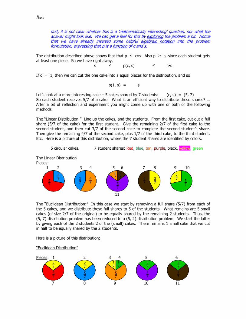
Let’s look at a more interesting case – 5 cakes shared by 7 students: (c, s) = (5, 7) So each student receives 5/7 of a cake. What is an efficient way to distribute these shares? … After a bit of reflection and experiment you might come up with one or both of the following methods. The “Linear Distribution:” Line up the cakes, and the students. From the first cake, cut out a full share (5/7 of the cake) for the first student. Give the remaining 2/7 of the first cake to the second student, and then cut 3/7 of the second cake to complete the second student’s share. Then give the remaining 4/7 of the second cake, plus 1/7 of the third cake, to the third student. Etc. Here is a picture of this distribution, where the 7 student shares are identified by colors.

5 circular cakes. 7 student shares: Red, blue, tan, purple, black, yellow, green The Linear Distribution Pieces: 1 2 3 4 5 6 7 8 9 10

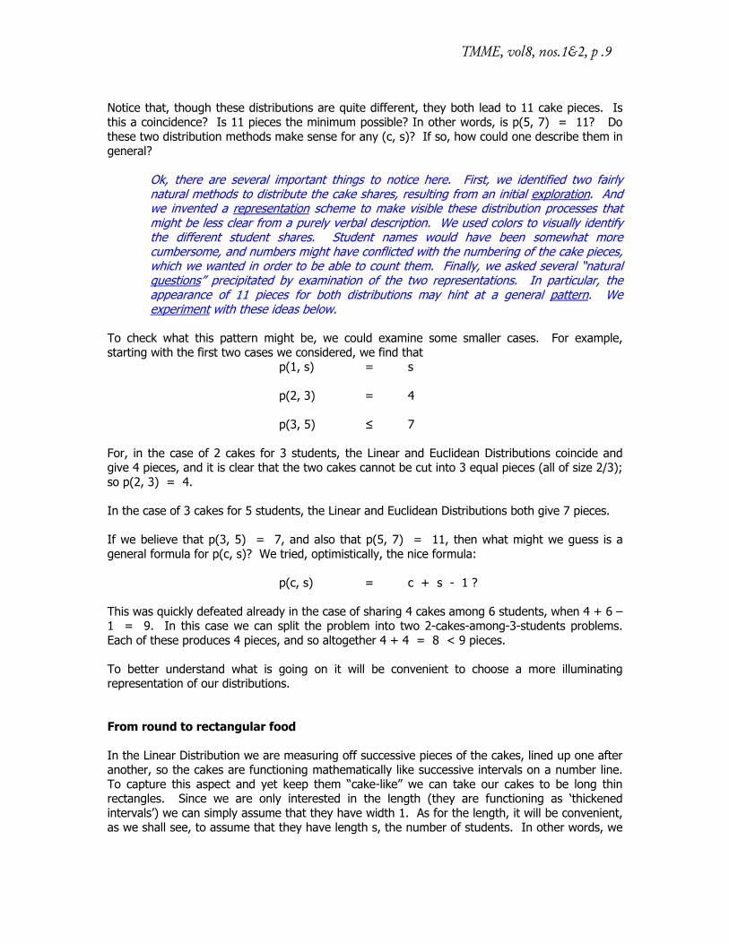
11 The “Euclidean Distribution:” In this case we start by removing a full share (5/7) from each of the 5 cakes, and we distribute these full shares to 5 of the students. What remains are 5 small cakes (of size 2/7 of the original) to be equally shared by the remaining 2 students. Thus, the (5, 7) distribution problem has been reduced to a (5, 2) distribution problem. We start the latter by giving each of the 2 students 2 of the (small) cakes. There remains 1 small cake that we cut in half to be equally shared by the 2 students. Here is a picture of this distribution; “Euclidean Distribution” Pieces: 1 2 3 4 5 6

7 8 9 10 11

TMME, vol8, nos.1&2, p .9

Notice that, though these distributions are quite different, they both lead to 11 cake pieces. Is this a coincidence? Is 11 pieces the minimum possible? In other words, is p(5, 7) = 11? Do these two distribution methods make sense for any (c, s)? If so, how could one describe them in general?

Ok, there are several important things to notice here. First, we identified two fairly natural methods to distribute the cake shares, resulting from an initial exploration. And we invented a representation scheme to make visible these distribution processes that might be less clear from a purely verbal description. We used colors to visually identify the different student shares. Student names would have been somewhat more cumbersome, and numbers might have conflicted with the numbering of the cake pieces, which we wanted in order to be able to count them. Finally, we asked several “natural questions” precipitated by examination of the two representations. In particular, the appearance of 11 pieces for both distributions may hint at a general pattern. We experiment with these ideas below.

To check what this pattern might be, we could examine some smaller cases. For example, starting with the first two cases we considered, we find that p(1, s) = s p(2, 3) = 4 p(3, 5) ≤ 7 For, in the case of 2 cakes for 3 students, the Linear and Euclidean Distributions coincide and give 4 pieces, and it is clear that the two cakes cannot be cut into 3 equal pieces (all of size 2/3); so p(2, 3) = 4. In the case of 3 cakes for 5 students, the Linear and Euclidean Distributions both give 7 pieces. If we believe that p(3, 5) = 7, and also that p(5, 7) = 11, then what might we guess is a general formula for p(c, s)? We tried, optimistically, the nice formula: p(c, s) = c + s - 1 ? This was quickly defeated already in the case of sharing 4 cakes among 6 students, when 4 + 6 – 1 = 9. In this case we can split the problem into two 2-cakes-among-3-students problems. Each of these produces 4 pieces, and so altogether 4 + 4 = 8 < 9 pieces. To better understand what is going on it will be convenient to choose a more illuminating representation of our distributions. From round to rectangular food In the Linear Distribution we are measuring off successive pieces of the cakes, lined up one after another, so the cakes are functioning mathematically like successive intervals on a number line. To capture this aspect and yet keep them “cake-like” we can take our cakes to be long thin rectangles. Since we are only interested in the length (they are functioning as ‘thickened intervals’) we can simply assume that they have width 1. As for the length, it will be convenient, as we shall see, to assume that they have length s, the number of students. In other words, we

Bass

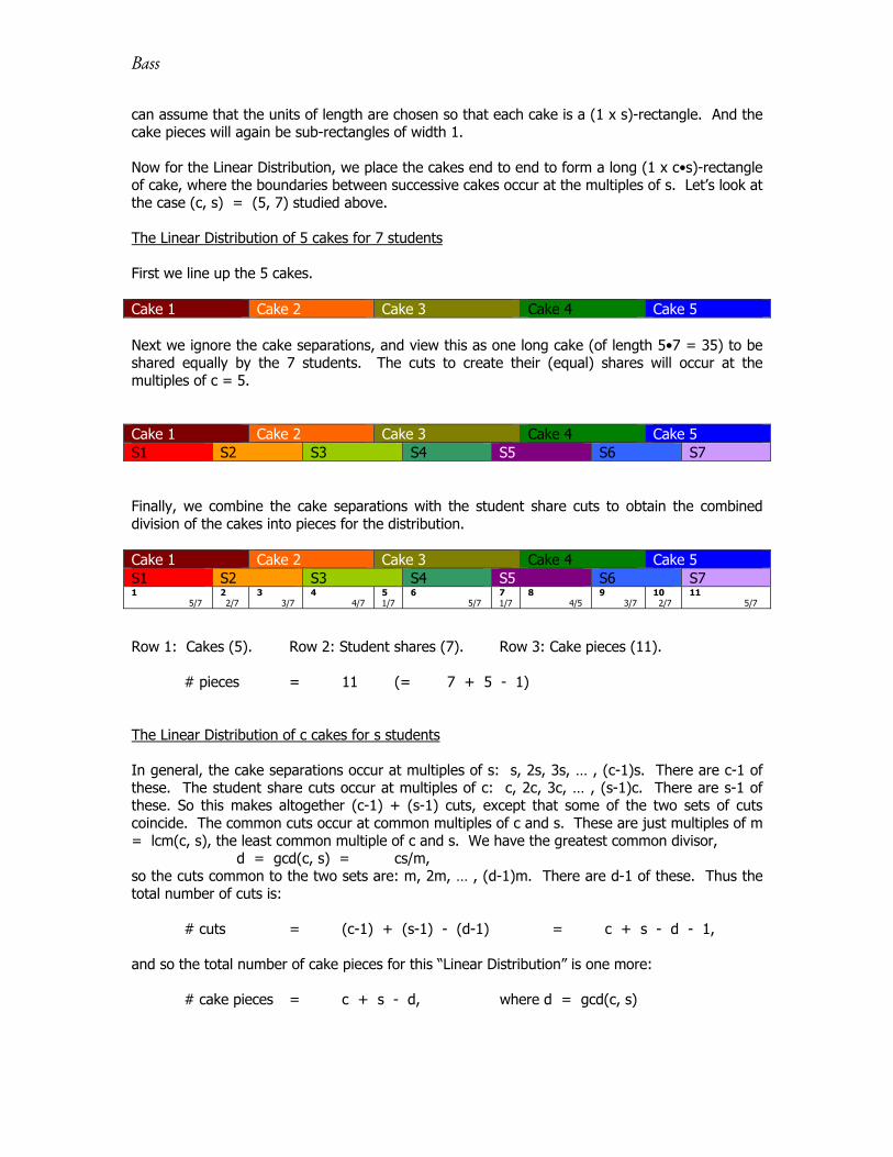
can assume that the units of length are chosen so that each cake is a (1 x s)-rectangle. And the cake pieces will again be sub-rectangles of width 1. Now for the Linear Distribution, we place the cakes end to end to form a long (1 x c•s)-rectangle of cake, where the boundaries between successive cakes occur at the multiples of s. Let’s look at the case (c, s) = (5, 7) studied above. The Linear Distribution of 5 cakes for 7 students First we line up the 5 cakes. Cake 1 Cake 2 Cake 3 Cake 4 Cake 5 Next we ignore the cake separations, and view this as one long cake (of length 5•7 = 35) to be shared equally by the 7 students. The cuts to create their (equal) shares will occur at the multiples of c = 5. Cake 1 Cake 2 Cake 3 Cake 4 Cake 5 S1 S2 S3 S4 S5 S6 S7 Finally, we combine the cake separations with the student share cuts to obtain the combined division of the cakes into pieces for the distribution. Cake 1 Cake 2 Cake 3 Cake 4 Cake 5 S1 S2 S3 S4 S5 S6 S7 1 5/7

2 2/7

3 3/7

4 4/7

51/7

6 5/7

71/7

8 4/5

9 3/7

10 2/7

11 5/7

Row 1: Cakes (5). Row 2: Student shares (7). Row 3: Cake pieces (11). # pieces = 11 (= 7 + 5 - 1) The Linear Distribution of c cakes for s students In general, the cake separations occur at multiples of s: s, 2s, 3s, … , (c-1)s. There are c-1 of these. The student share cuts occur at multiples of c: c, 2c, 3c, … , (s-1)c. There are s-1 of these. So this makes altogether (c-1) + (s-1) cuts, except that some of the two sets of cuts coincide. The common cuts occur at common multiples of c and s. These are just multiples of m = lcm(c, s), the least common multiple of c and s. We have the greatest common divisor, d = gcd(c, s) = cs/m, so the cuts common to the two sets are: m, 2m, … , (d-1)m. There are d-1 of these. Thus the total number of cuts is: # cuts = (c-1) + (s-1) - (d-1) = c + s - d - 1, and so the total number of cake pieces for this “Linear Distribution” is one more: # cake pieces = c + s - d, where d = gcd(c, s)

TMME, vol8, nos.1&2, p .11

Of course we see here a significantly new (rectangular) representation of the Linear Distribution, one that better coordinates the geometry of the representation with the arithmetic of the distribution. Moreover, this representation makes easily available (and visualizable) an analysis of the number of pieces, as a function of c and s. We could see the structure in the (5, 7) case, and this guided the analysis in the general case. (Notice also that, from the point of view of this analysis, there is a certain symmetry in the roles of c and s.) And it raises the “natural next question:” “Can we do something similar for the Euclidean Distribution?”

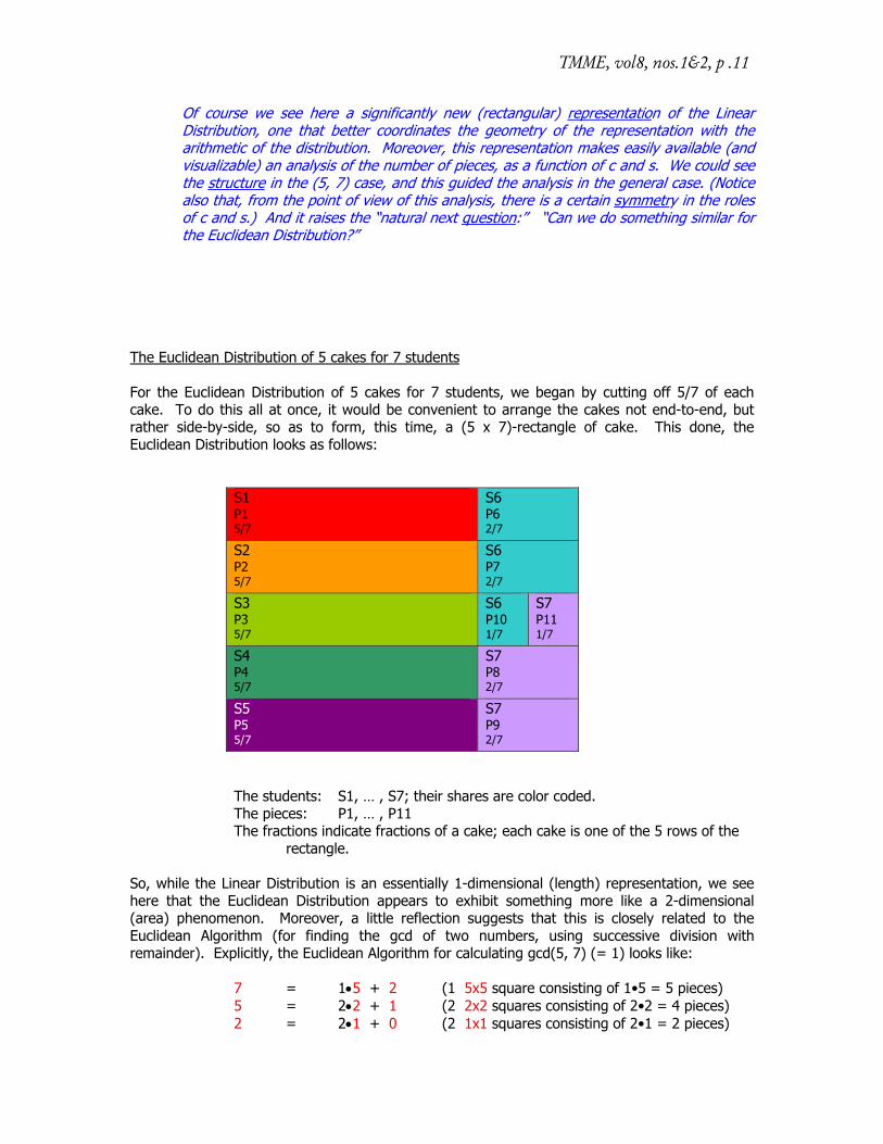
The Euclidean Distribution of 5 cakes for 7 students For the Euclidean Distribution of 5 cakes for 7 students, we began by cutting off 5/7 of each cake. To do this all at once, it would be convenient to arrange the cakes not end-to-end, but rather side-by-side, so as to form, this time, a (5 x 7)-rectangle of cake. This done, the Euclidean Distribution looks as follows:

S1 P1 5/7

S6 P6 2/7

S2 P2 5/7

S6 P7 2/7

S3 P3 5/7

S6 P10 1/7

S7 P11 1/7

S4 P4 5/7

S7 P8 2/7

S5 P5 5/7

S7 P9 2/7

The students: S1, … , S7; their shares are color coded. The pieces: P1, … , P11 The fractions indicate fractions of a cake; each cake is one of the 5 rows of the rectangle. So, while the Linear Distribution is an essentially 1-dimensional (length) representation, we see here that the Euclidean Distribution appears to exhibit something more like a 2-dimensional (area) phenomenon. Moreover, a little reflection suggests that this is closely related to the Euclidean Algorithm (for finding the gcd of two numbers, using successive division with remainder). Explicitly, the Euclidean Algorithm for calculating gcd(5, 7) (= 1) looks like: 7 = 15 + 2 (1 5x5 square consisting of 1•5 = 5 pieces) 5 = 22 + 1 (2 2x2 squares consisting of 2•2 = 4 pieces) 2 = 21 + 0 (2 1x1 squares consisting of 2•1 = 2 pieces)

Bass

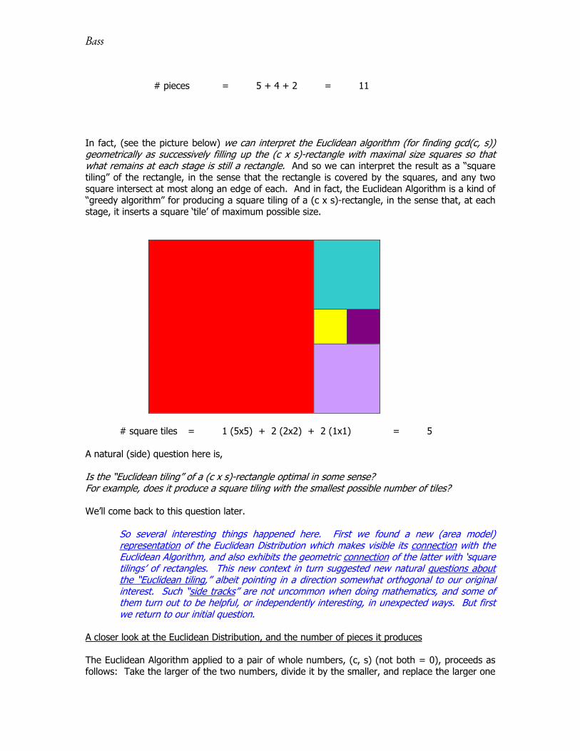
# pieces = 5 + 4 + 2 = 11 In fact, (see the picture below) we can interpret the Euclidean algorithm (for finding gcd(c, s)) geometrically as successively filling up the (c x s)-rectangle with maximal size squares so that what remains at each stage is still a rectangle. And so we can interpret the result as a “square tiling” of the rectangle, in the sense that the rectangle is covered by the squares, and any two square intersect at most along an edge of each. And in fact, the Euclidean Algorithm is a kind of “greedy algorithm” for producing a square tiling of a (c x s)-rectangle, in the sense that, at each stage, it inserts a square ‘tile’ of maximum possible size.

# square tiles = 1 (5x5) + 2 (2x2) + 2 (1x1) = 5 A natural (side) question here is, Is the “Euclidean tiling” of a (c x s)-rectangle optimal in some sense? For example, does it produce a square tiling with the smallest possible number of tiles? We’ll come back to this question later.

So several interesting things happened here. First we found a new (area model) representation of the Euclidean Distribution which makes visible its connection with the Euclidean Algorithm, and also exhibits the geometric connection of the latter with ‘square tilings’ of rectangles. This new context in turn suggested new natural questions about the “Euclidean tiling,” albeit pointing in a direction somewhat orthogonal to our original interest. Such “side tracks” are not uncommon when doing mathematics, and some of them turn out to be helpful, or independently interesting, in unexpected ways. But first we return to our initial question.

A closer look at the Euclidean Distribution, and the number of pieces it produces The Euclidean Algorithm applied to a pair of whole numbers, (c, s) (not both = 0), proceeds as follows: Take the larger of the two numbers, divide it by the smaller, and replace the larger one

TMME, vol8, nos.1&2, p .13

by the remainder in this division. After a finite number of such steps, one of the two numbers will be zero, and then the non-zero remaining number is the gcd(c, s). More explicitly, and with interpretation for the cake distribution, we have the following cases:

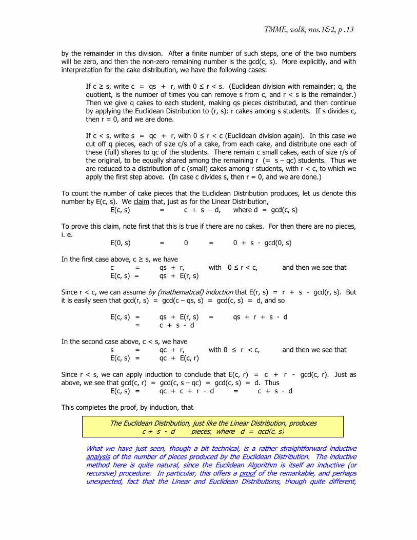
If c ≥ s, write c = qs + r, with 0 ≤ r < s. (Euclidean division with remainder; q, the quotient, is the number of times you can remove s from c, and r < s is the remainder.) Then we give q cakes to each student, making qs pieces distributed, and then continue by applying the Euclidean Distribution to (r, s): r cakes among s students. If s divides c, then r = 0, and we are done. If c < s, write s = qc + r, with 0 ≤ r < c (Euclidean division again). In this case we cut off q pieces, each of size c/s of a cake, from each cake, and distribute one each of these (full) shares to qc of the students. There remain c small cakes, each of size r/s of the original, to be equally shared among the remaining r (= s – qc) students. Thus we are reduced to a distribution of c (small) cakes among r students, with r < c, to which we apply the first step above. (In case c divides s, then r = 0, and we are done.)

To count the number of cake pieces that the Euclidean Distribution produces, let us denote this number by E(c, s). We claim that, just as for the Linear Distribution, E(c, s) = c + s - d, where d = gcd(c, s) To prove this claim, note first that this is true if there are no cakes. For then there are no pieces, i. e. E(0, s) = 0 = 0 + s - gcd(0, s) In the first case above, c ≥ s, we have c = qs + r, with 0 ≤ r < c, and then we see that E(c, s) = qs + E(r, s) Since r < c, we can assume by (mathematical) induction that E(r, s) = r + s - gcd(r, s). But it is easily seen that gcd(r, s) = gcd(c – qs, s) = gcd(c, s) = d, and so E(c, s) = qs + E(r, s) = qs + r + s - d = c + s - d In the second case above, c < s, we have s = qc + r, with 0 ≤ r < c, and then we see that E(c, s) = qc + E(c, r) Since r < s, we can apply induction to conclude that E(c, r) = c + r - gcd(c, r). Just as above, we see that gcd(c, r) = gcd(c, s – qc) = gcd(c, s) = d. Thus E(c, s) = qc + c + r - d = c + s - d This completes the proof, by induction, that

What we have just seen, though a bit technical, is a rather straightforward inductive analysis of the number of pieces produced by the Euclidean Distribution. The inductive method here is quite natural, since the Euclidean Algorithm is itself an inductive (or recursive) procedure. In particular, this offers a proof of the remarkable, and perhaps unexpected, fact that the Linear and Euclidean Distributions, though quite different,

The Euclidean Distribution, just like the Linear Distribution, produces c + s - d pieces, where d = gcd(c, s)

Bass

produce the same number of pieces, c + s - d, thus establishing an interesting connection. This makes the number c + s – d seem quite special to the cake distribution problem, and strongly tempts us to make the:

In other words, the smallest number, p(c, s), of cake pieces you can use to share c cakes among s students is c + s - d. We have already seen, with the Linear and Euclidean Distributions use exactly c + s - d pieces, and so p(c, s) ≤ c + s - d

Side comment on the Euclidean Algorithm: The school curriculum often gives diminished attention to ‘long division’ (here called Euclidean division), and therefore also small attention (if any) to the Euclidean Algorithm for finding the gcd(c, s) = d of two whole numbers c and s, which is based on Euclidean division. The method generally offered is to first find the prime factorizations of c and s, and then simply inspect these to find d. And in fact, for small numbers, this is likely most efficient. However, if nothing more is said, this deprives students of the awareness, in comparing the two methods – Euclidean Algorithm vs. prime factorization – in general, that for large numbers (say > 6 digits), the problem of prime factorization becomes an intractably difficult computation, whereas the Euclidean Algorithm, despite appearances, is relatively straightforward and can be done in practical (‘polynomial’) computational time relative to the size of c and s. This phenomenon is fundamentally important in cryptography. Thus, ironically, neglecting long division, often done on the grounds that we have calculators to do such computations, will deprive students of exposure to an important idea about complexity of computations that is central to modern computer science.

Seeking a proof of the Conjecture: A side trip into graph theory It remains to show (in order to prove the Conjecture above) that we can’t do better, i.e. distribute c cakes to s students with fewer than c + s – d pieces. In other words, it remains to show that, p(c, s) ≥ c + s - d How can we possibly show this? It is here that we shall push the envelope of school mathematics a bit. So far, we have been using fairly basic, though substantial, mathematical ideas and tools of High School mathematics. I think it is fair to say that most mathematicians who spent some serious time thinking about this question would arrive eventually at the point we are at now. But the next steps seem less predictable. At this point, after considerable reflection, I had to reach for a new connection. The graph of a cake distribution The problem now is that we have to consider any possible distribution D of c cakes to s students, and show that D must consist of at least c + s – d pieces. In contrast with our discussion of the Linear and Euclidean Distributions, we have no special information about D. So let’s think a bit about what D is. D distributes cake pieces to students. So one way to picture this schematically is as follows. For each cake piece, draw a line from the cake from which it came, to the student

Main Conjecture: p(c, s) = c + s - d, where d = gcd(c, s)

TMME, vol8, nos.1&2, p .15

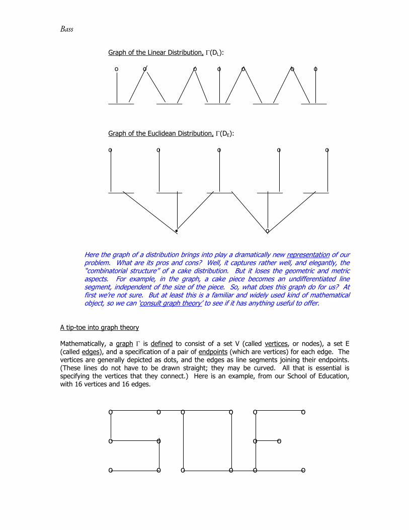
to whom it is given. If we forget that the cakes are cakes, and that the students are people, and simply represent them abstractly as dots, then what we have is a collection of dots, together with some lines (corresponding to the cake pieces) connecting various pairs of these dots. This is in fact a familiar kind of mathematical object, called a (combinatorial) graph. We shall call this the graph of the distribution D, and denote it (D). To see what this looks like, consider the graphs of the Linear Distribution DL and the Euclidean Distribution DE, for c = 5 and s = 7. We shall represent the students by dots, and the cakes by short horizontal line segments instead of dots, just to be a bit more suggestive of the context.

Bass

Graph of the Linear Distribution, (DL): o o o o o o o

_______ _______ _______ _______ _______

Graph of the Euclidean Distribution, (DE): o o o o o

_______ _______ _______ _______ _______

o

Here the graph of a distribution brings into play a dramatically new representation of our problem. What are its pros and cons? Well, it captures rather well, and elegantly, the “combinatorial structure” of a cake distribution. But it loses the geometric and metric aspects. For example, in the graph, a cake piece becomes an undifferentiated line segment, independent of the size of the piece. So, what does this graph do for us? At first we’re not sure. But at least this is a familiar and widely used kind of mathematical object, so we can ‘consult graph theory’ to see if it has anything useful to offer.

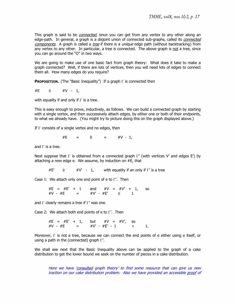
A tip-toe into graph theory Mathematically, a graph is defined to consist of a set V (called vertices, or nodes), a set E (called edges), and a specification of a pair of endpoints (which are vertices) for each edge. The vertices are generally depicted as dots, and the edges as line segments joining their endpoints. (These lines do not have to be drawn straight; they may be curved. All that is essential is specifying the vertices that they connect.) Here is an example, from our School of Education, with 16 vertices and 16 edges.

o o o o o o o o o o o o o o o o

TMME, vol8, nos.1&2, p .17

This graph is said to be connected, since you can get from any vertex to any other along an edge-path. In general, a graph is a disjoint union of connected sub-graphs, called its connected components. A graph is called a tree if there is a unique edge path (without backtracking) from any vertex to any other. In particular, a tree is connected. The above graph is not a tree, since you can go around the “O” in two ways. We are going to make use of one basic fact from graph theory: What does it take to make a graph connected? Well, if there are lots of vertices, then you will need lots of edges to connect them all. How many edges do you require? PROPOSITION. (The “Basic Inequality”) If a graph is connected then #E ≥ #V - 1, with equality if and only if is a tree. This is easy enough to prove, inductively, as follows. We can build a connected graph by starting with a single vertex, and then successively attach edges, by either one or both of their endpoints, to what we already have. (You might try to picture doing this on the graph displayed above.) If consists of a single vertex and no edges, then #E = 0 = #V - 1, and is a tree. Next suppose that is obtained from a connected graph ’ (with vertices V’ and edges E’) by attaching a new edge e. We assume, by induction on #E, that #E’ ≥ #V’ - 1, with equality if an only if ’ is a tree Case 1: We attach only one end point of e to ’. Then #E = #E’ + 1 and #V = #V’ + 1, so #V - #E = #V’ - #E’ ≤ 1 and clearly remains a tree if ’ was one. Case 2: We attach both end points of e to ’. Then #E = #E’ + 1, but #V = #V’, so #V - #E = #V’ - #E’ - 1 < 1. Moreover, is not a tree, because we can connect the end points of e either using e itself, or using a path in the (connected) graph ’. We shall see next that the Basic Inequality above can be applied to the graph of a cake distribution to get the lower bound we seek on the number of pieces in a cake distribution.

Here we have ‘consulted graph theory’ to find some resource that can give us new traction on our cake distribution problem. Also we have provided an accessible proof of

Bass

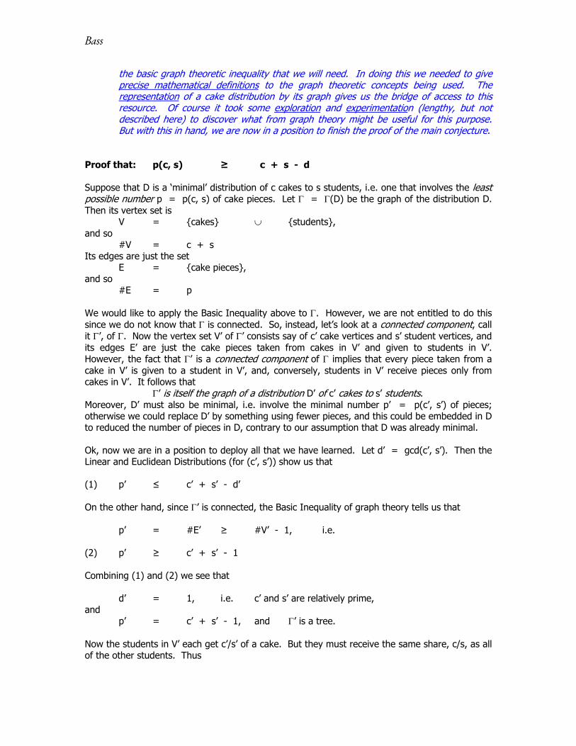
the basic graph theoretic inequality that we will need. In doing this we needed to give precise mathematical definitions to the graph theoretic concepts being used. The representation of a cake distribution by its graph gives us the bridge of access to this resource. Of course it took some exploration and experimentation (lengthy, but not described here) to discover what from graph theory might be useful for this purpose. But with this in hand, we are now in a position to finish the proof of the main conjecture.

Proof that: p(c, s) ≥ c + s - d Suppose that D is a ‘minimal’ distribution of c cakes to s students, i.e. one that involves the least possible number p = p(c, s) of cake pieces. Let = (D) be the graph of the distribution D. Then its vertex set is V = {cakes} {students}, and so #V = c + s Its edges are just the set E = {cake pieces}, and so #E = p We would like to apply the Basic Inequality above to . However, we are not entitled to do this since we do not know that is connected. So, instead, let’s look at a connected component, call it ’, of . Now the vertex set V’ of ’ consists say of c’ cake vertices and s’ student vertices, and its edges E’ are just the cake pieces taken from cakes in V’ and given to students in V’. However, the fact that ’ is a connected component of implies that every piece taken from a cake in V’ is given to a student in V’, and, conversely, students in V’ receive pieces only from cakes in V’. It follows that ’ is itself the graph of a distribution D’ of c’ cakes to s’ students. Moreover, D’ must also be minimal, i.e. involve the minimal number p’ = p(c’, s’) of pieces; otherwise we could replace D’ by something using fewer pieces, and this could be embedded in D to reduced the number of pieces in D, contrary to our assumption that D was already minimal. Ok, now we are in a position to deploy all that we have learned. Let d’ = gcd(c’, s’). Then the Linear and Euclidean Distributions (for (c’, s’)) show us that (1) p’ ≤ c’ + s’ - d’ On the other hand, since ’ is connected, the Basic Inequality of graph theory tells us that p’ = #E’ ≥ #V’ - 1, i.e. (2) p’ ≥ c’ + s’ - 1 Combining (1) and (2) we see that d’ = 1, i.e. c’ and s’ are relatively prime, and p’ = c’ + s’ - 1, and ’ is a tree. Now the students in V’ each get c’/s’ of a cake. But they must receive the same share, c/s, as all of the other students. Thus

TMME, vol8, nos.1&2, p .19

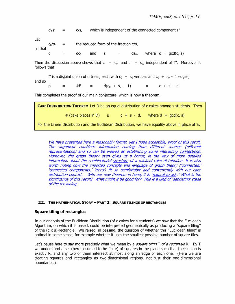
c’/s’ = c/s, which is independent of the connected component ’ Let c0/s0 = the reduced form of the fraction c/s, so that c = dc0 and s = ds0, where d = gcd(c, s) Then the discussion above shows that c’ = c0 and s’ = s0, independent of ’. Moreover it follows that is a disjoint union of d trees, each with c0 + s0 vertices and c0 + s0 - 1 edges, and so p = #E = d(c0 + s0 - 1) = c + s - d This completes the proof of our main conjecture, which is now a theorem.

We have presented here a reasonably formal, yet I hope accessible, proof of this result. The argument combines information coming from different sources (different representations) and so can be viewed as establishing some interesting connections. Moreover, the graph theory even gives us a bonus, in the way of more detailed information about the combinatorial structure of a minimal cake distribution. It is also worth noting how the imported concepts and language of graph theory (‘connected,’ ‘connected components,’ ‘trees’) fit so comfortably and conveniently with our cake distribution context. With our new theorem in hand, it is “natural to ask:” What is the significance of this result? What might it be good for? This is a kind of ‘debriefing’ stage of the reasoning.

III. THE MATHEMATICAL STORY – PART 2: SQUARE TILINGS OF RECTANGLES Square tiling of rectangles In our analysis of the Euclidean Distribution (of c cakes for s students) we saw that the Euclidean Algorithm, on which it is based, could be interpreted geometrically as producing a “square tiling” of the (c x s)-rectangle. We raised, in passing, the question of whether this “Euclidean tiling” is optimal in some sense, for example whether it uses the smallest possible number of square tiles. Let’s pause here to say more precisely what we mean by a square tiling T of a rectangle R. By T we understand a set (here assumed to be finite) of squares in the plane such that their union is exactly R, and any two of them intersect at most along an edge of each one. (Here we are treating squares and rectangles as two-dimensional regions, not just their one-dimensional boundaries.)

CAKE DISTRIBUTION THEOREM Let D be an equal distribution of c cakes among s students. Then # (cake pieces in D) ≥ c + s - d, where d = gcd(c, s) For the Linear Distribution and the Euclidean Distribution, we have equality above in place of ≥.

Bass

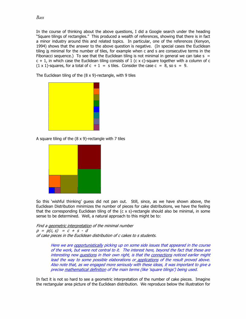
In the course of thinking about the above questions, I did a Google search under the heading “Square tilings of rectangles.” This produced a wealth of references, showing that there is in fact a minor industry around this and related topics. In particular, one of the references (Kenyon, 1994) shows that the answer to the above question is negative. (In special cases the Euclidean tiling is minimal for the number of tiles, for example when c and s are consecutive terms in the Fibonacci sequence.) To see that the Euclidean tiling is not minimal in general we can take s = c + 1, in which case the Euclidean tiling consists of 1 (c x c)-square together with a column of c (1 x 1)-squares, for a total of c + 1 = s tiles. Consider the case c = 8, so s = 9. The Euclidean tiling of the (8 x 9)-rectangle, with 9 tiles

A square tiling of the (8 x 9)-rectangle with 7 tiles

So this ‘wishful thinking’ guess did not pan out. Still, since, as we have shown above, the Euclidean Distribution minimizes the number of pieces for cake distributions, we have the feeling that the corresponding Euclidean tiling of the (c x s)-rectangle should also be minimal, in some sense to be determined. Well, a natural approach to this might be to: Find a geometric interpretation of the minimal number p = p(c, s) = c + s - d of cake pieces in the Euclidean distribution of c cakes to s students.

Here we are opportunistically picking up on some side issues that appeared in the course of the work, but were not central to it. The interest here, beyond the fact that these are interesting new questions in their own right, is that the connections noticed earlier might lead the way to some possible elaborations or applications of the result proved above. Also note that, as we engaged more seriously with these ideas, it was important to give a precise mathematical definition of the main terms (like ‘square tilings’) being used.

In fact it is not so hard to see a geometric interpretation of the number of cake pieces. Imagine the rectangular area picture of the Euclidean distribution. We reproduce below the illustration for

TMME, vol8, nos.1&2, p .21

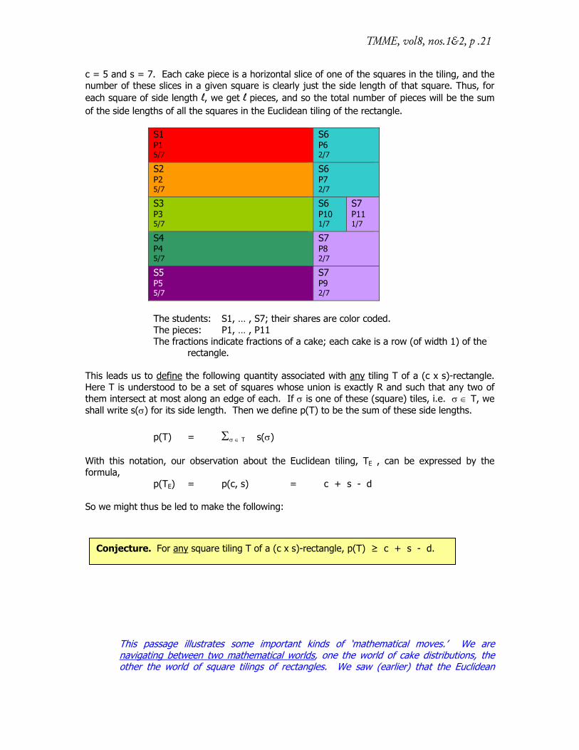
c = 5 and s = 7. Each cake piece is a horizontal slice of one of the squares in the tiling, and the number of these slices in a given square is clearly just the side length of that square. Thus, for each square of side length l, we get l pieces, and so the total number of pieces will be the sum of the side lengths of all the squares in the Euclidean tiling of the rectangle.

S1 P1 5/7

S6 P6 2/7

S2 P2 5/7

S6 P7 2/7

S3 P3 5/7

S6 P10 1/7

S7 P11 1/7

S4 P4 5/7

S7 P8 2/7

S5 P5 5/7

S7 P9 2/7

The students: S1, … , S7; their shares are color coded. The pieces: P1, … , P11 The fractions indicate fractions of a cake; each cake is a row (of width 1) of the rectangle. This leads us to define the following quantity associated with any tiling T of a (c x s)-rectangle. Here T is understood to be a set of squares whose union is exactly R and such that any two of them intersect at most along an edge of each. If is one of these (square) tiles, i.e. T, we shall write s() for its side length. Then we define p(T) to be the sum of these side lengths.

p(T) = T s() With this notation, our observation about the Euclidean tiling, TE , can be expressed by the formula, p(TE) = p(c, s) = c + s - d So we might thus be led to make the following:

This passage illustrates some important kinds of ‘mathematical moves.’ We are navigating between two mathematical worlds, one the world of cake distributions, the other the world of square tilings of rectangles. We saw (earlier) that the Euclidean

Conjecture. For any square tiling T of a (c x s)-rectangle, p(T) ≥ c + s - d.

Bass

Distribution established a bridge between these two worlds, the Euclidean Distribution at one end, the Euclidean tiling at the other. We proved that the Euclidean Distribution has a minimizing property in the cake distribution world, so we were tempted to ask if (or suspect that) the Euclidean tiling has some analogous minimizing property. This is a kind of reasoning by analogy that mathematicians often use, to guess what might be true, by developing a relation of some new situation to an old one, about which we already know something. It can be viewed as another kind of pattern seeking. The procedure we followed was to try to build up the dictionary of translation from the cake world to the tiling world. Given that [Euclidean Distribution] translates to [Euclidean tiling], we ask, [# pieces] translate to [???]. What we seek here is something that we can measure geometrically for all tilings in the tiling world, and so that, when applied to the Euclidean tiling, gives something closely related to the number (c + s – d) of pieces. We found p(T) as the answer to that question, and accordingly we gave it a name, p(T), so that we could talk about and work with it.

The Conjecture above, if true, would indeed show that the Euclidean tiling minimizes p(T), and so it is geometrically optimal among tilings, in this sense. Can we prove this Conjecture? The geometric statement is not so obvious. Perhaps, instead of directly attacking it geometrically, we can use our Cake Distribution Theorem to help. In other words, perhaps we can interpret any square tiling T of a (c x s)-rectangle as arising somehow from a cake distribution of c cakes among s students, and in such a way that p(T) is the number of cake pieces. If we can do that, then we will have proved the above conjecture by reducing it to the Cake Distribution Theorem.

So here we are proposing to show that our dictionary is (at least partly) reversible; in other words we can go back from a square tiling to a cake distribution. In this way, we can use our dictionary to import our theorem on cake distributions to the tiling world, where it translates into a geometric theorem.

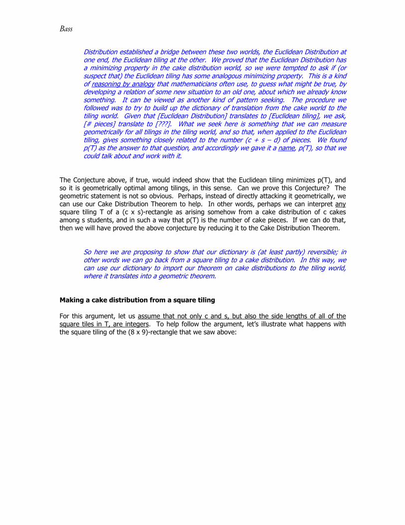
Making a cake distribution from a square tiling For this argument, let us assume that not only c and s, but also the side lengths of all of the square tiles in T, are integers. To help follow the argument, let’s illustrate what happens with the square tiling of the (8 x 9)-rectangle that we saw above:

TMME, vol8, nos.1&2, p .23

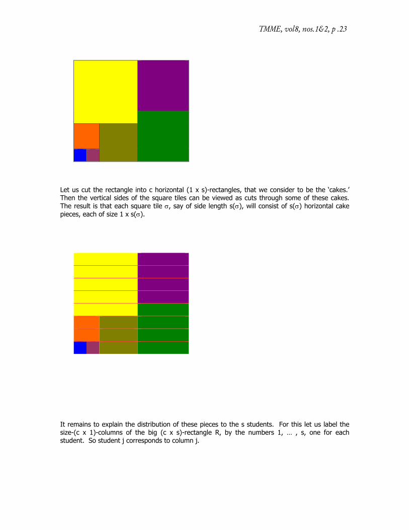
Let us cut the rectangle into c horizontal (1 x s)-rectangles, that we consider to be the ‘cakes.’ Then the vertical sides of the square tiles can be viewed as cuts through some of these cakes. The result is that each square tile , say of side length s(), will consist of s() horizontal cake pieces, each of size 1 x s().

It remains to explain the distribution of these pieces to the s students. For this let us label the size-(c x 1)-columns of the big (c x s)-rectangle R, by the numbers 1, … , s, one for each student. So student j corresponds to column j.

Bass

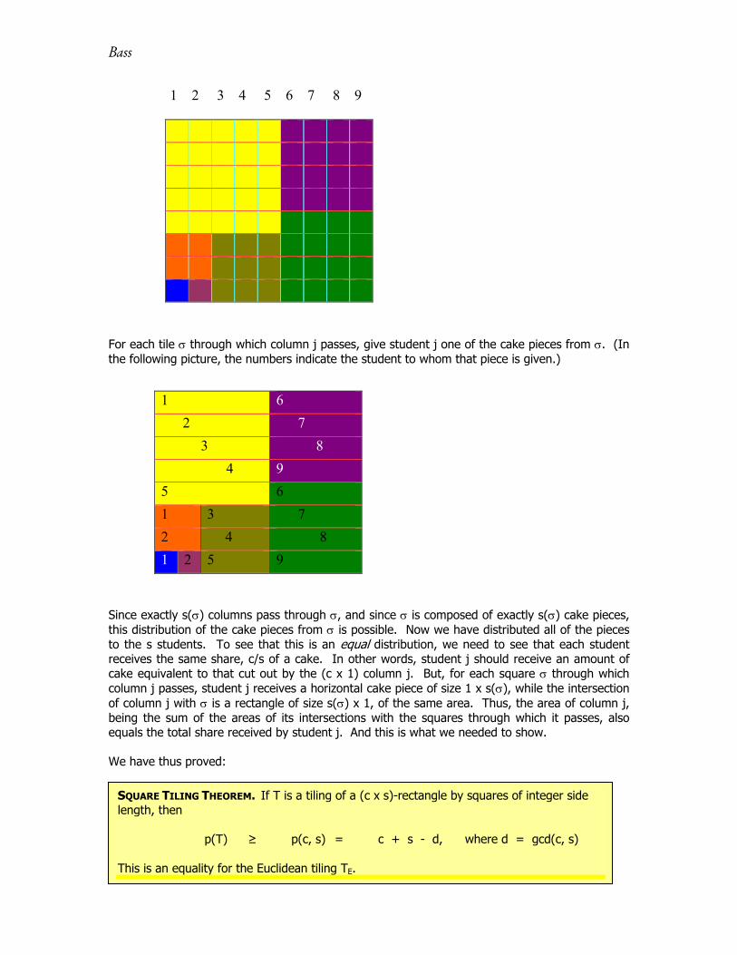
1 2 3 4 5 6 7 8 9 For each tile through which column j passes, give student j one of the cake pieces from . (In the following picture, the numbers indicate the student to whom that piece is given.) Since exactly s() columns pass through , and since is composed of exactly s() cake pieces, this distribution of the cake pieces from is possible. Now we have distributed all of the pieces to the s students. To see that this is an equal distribution, we need to see that each student receives the same share, c/s of a cake. In other words, student j should receive an amount of cake equivalent to that cut out by the (c x 1) column j. But, for each square through which column j passes, student j receives a horizontal cake piece of size 1 x s(), while the intersection of column j with is a rectangle of size s() x 1, of the same area. Thus, the area of column j, being the sum of the areas of its intersections with the squares through which it passes, also equals the total share received by student j. And this is what we needed to show. We have thus proved:

1 6

2 7

3 8

4 9

5 6

1 3 7

2 4 8

1 2 5 9

SQUARE TILING THEOREM. If T is a tiling of a (c x s)-rectangle by squares of integer side length, then p(T) ≥ p(c, s) = c + s - d, where d = gcd(c, s) This is an equality for the Euclidean tiling TE.

TMME, vol8, nos.1&2, p .25

So this is a satisfying outcome, but with the one caveat that we had to restrict attention to square tiles of integer side length. We’ll come back to that issue later, but just take note of it now. The proof has, I think, a very nice ‘fit’ to it. It shows I think a close structural relation between square tilings and cake distributions, so that results about the latter have applications to the former. The proof above seems ‘natural enough,’ even though it is a bit tricky to explain (especially without the pictures). The key was finding the idea for the proof, not its execution. I have not found a direct geometric proof of the theorem above.

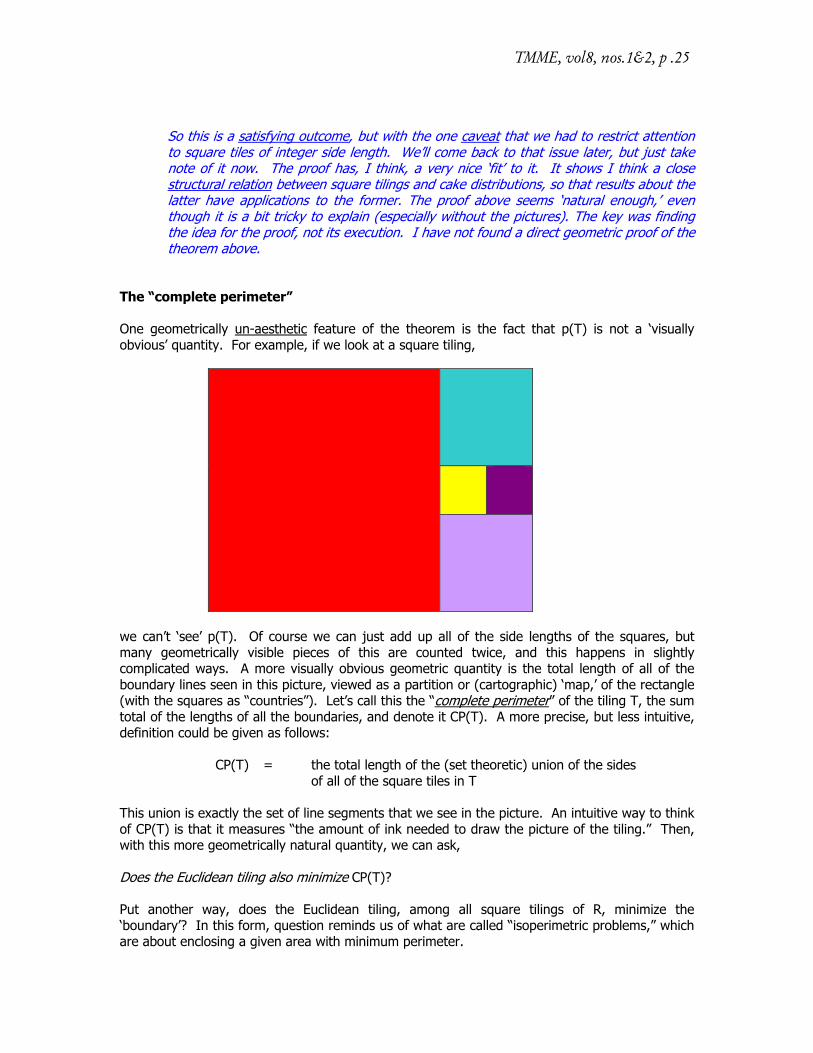
The “complete perimeter” One geometrically un-aesthetic feature of the theorem is the fact that p(T) is not a ‘visually obvious’ quantity. For example, if we look at a square tiling,

we can’t ‘see’ p(T). Of course we can just add up all of the side lengths of the squares, but many geometrically visible pieces of this are counted twice, and this happens in slightly complicated ways. A more visually obvious geometric quantity is the total length of all of the boundary lines seen in this picture, viewed as a partition or (cartographic) ‘map,’ of the rectangle (with the squares as “countries”). Let’s call this the “complete perimeter” of the tiling T, the sum total of the lengths of all the boundaries, and denote it CP(T). A more precise, but less intuitive, definition could be given as follows: CP(T) = the total length of the (set theoretic) union of the sides of all of the square tiles in T This union is exactly the set of line segments that we see in the picture. An intuitive way to think of CP(T) is that it measures “the amount of ink needed to draw the picture of the tiling.” Then, with this more geometrically natural quantity, we can ask, Does the Euclidean tiling also minimize CP(T)? Put another way, does the Euclidean tiling, among all square tilings of R, minimize the ‘boundary’? In this form, question reminds us of what are called “isoperimetric problems,” which are about enclosing a given area with minimum perimeter.

Bass

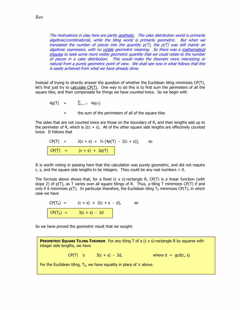
The motivations in play here are partly aesthetic. The cake distribution world is primarily algebraic/combinatorial, while the tiling world is primarily geometric. But when we translated the number of pieces into the quantity p(T), the p(T) was still mainly an algebraic expression, with no visible geometric meaning. So there was a mathematical impulse to seek some more visibly geometric quantity that we could relate to the number of pieces in a cake distribution. This would make the theorem more interesting or natural from a purely geometric point of view. We shall see now in what follows that this is easily achieved from what we have already done.

Instead of trying to directly answer the question of whether the Euclidean tiling minimizes CP(T), let’s first just try to calculate CP(T). One way to do this is to first sum the perimeters of all the square tiles, and then compensate for things we have counted twice. So we begin with

4p(T) = T 4s() = the sum of the perimeters of all of the square tiles The sides that are not counted twice are those on the boundary of R, and their lengths add up to the perimeter of R, which is 2(c + s). All of the other square side lengths are effectively counted twice. It follows that CP(T) = 2(c + s) + ½ [4p(T) - 2(c + s)], so It is worth noting in passing here that this calculation was purely geometric, and did not require c, s, and the square side lengths to be integers. They could be any real numbers > 0. The formula above shows that, for a fixed (c x s)-rectangle R, CP(T) is a linear function (with slope 2) of p(T), as T varies over all square tilings of R. Thus, a tiling T minimizes CP(T) if and only if it minimizes p(T). In particular therefore, the Euclidean tiling TE minimizes CP(T), in which case we have CP(TE) = (c + s) + 2(c + s - d), so

So we have proved the geometric result that we sought:

CP(T) = (c + s) + 2p(T)

CP(TE) = 3(c + s) - 2d

PERIMETRIC SQUARE TILING THEOREM For any tiling T of a (c x s)-rectangle R by squares with integer side lengths, we have CP(T) ≥ 3(c + s) - 2d, where d = gcd(c, s) For the Euclidean tiling, TE, we have equality in place of ≥ above.

TMME, vol8, nos.1&2, p .27

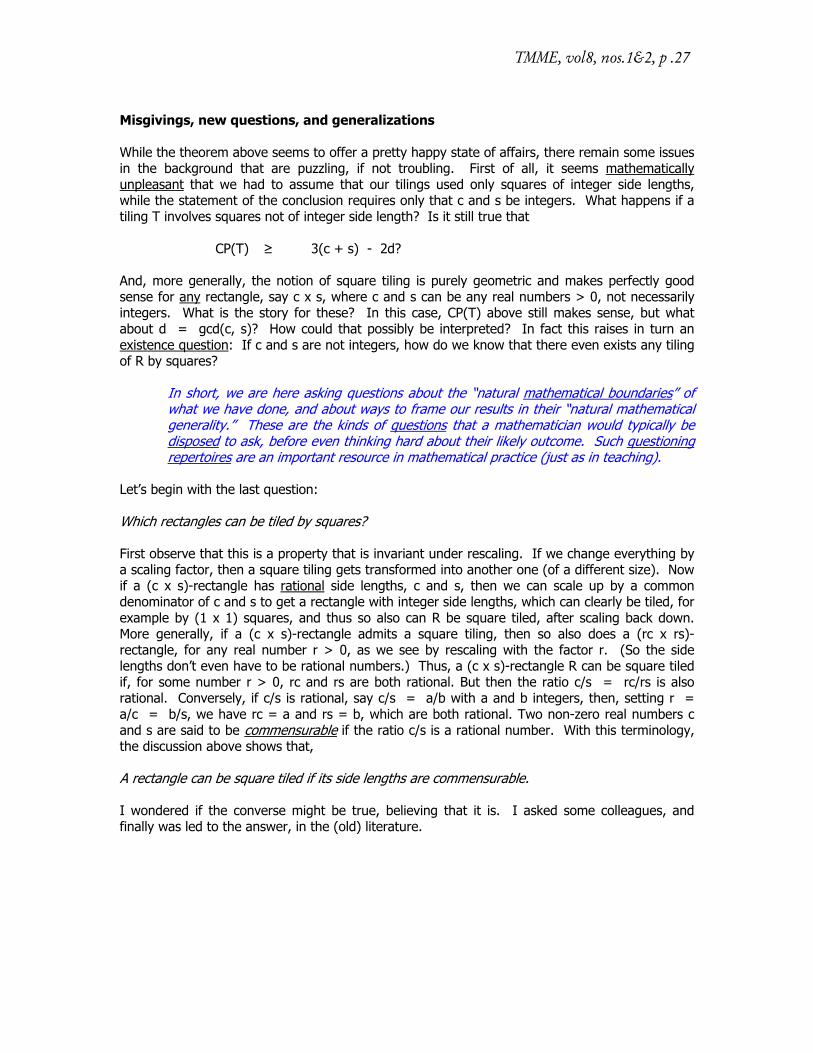
Misgivings, new questions, and generalizations While the theorem above seems to offer a pretty happy state of affairs, there remain some issues in the background that are puzzling, if not troubling. First of all, it seems mathematically unpleasant that we had to assume that our tilings used only squares of integer side lengths, while the statement of the conclusion requires only that c and s be integers. What happens if a tiling T involves squares not of integer side length? Is it still true that CP(T) ≥ 3(c + s) - 2d? And, more generally, the notion of square tiling is purely geometric and makes perfectly good sense for any rectangle, say c x s, where c and s can be any real numbers > 0, not necessarily integers. What is the story for these? In this case, CP(T) above still makes sense, but what about d = gcd(c, s)? How could that possibly be interpreted? In fact this raises in turn an existence question: If c and s are not integers, how do we know that there even exists any tiling of R by squares?

In short, we are here asking questions about the “natural mathematical boundaries” of what we have done, and about ways to frame our results in their “natural mathematical generality.” These are the kinds of questions that a mathematician would typically be disposed to ask, before even thinking hard about their likely outcome. Such questioning repertoires are an important resource in mathematical practice (just as in teaching).

Let’s begin with the last question: Which rectangles can be tiled by squares? First observe that this is a property that is invariant under rescaling. If we change everything by a scaling factor, then a square tiling gets transformed into another one (of a different size). Now if a (c x s)-rectangle has rational side lengths, c and s, then we can scale up by a common denominator of c and s to get a rectangle with integer side lengths, which can clearly be tiled, for example by (1 x 1) squares, and thus so also can R be square tiled, after scaling back down. More generally, if a (c x s)-rectangle admits a square tiling, then so also does a (rc x rs)-rectangle, for any real number r > 0, as we see by rescaling with the factor r. (So the side lengths don’t even have to be rational numbers.) Thus, a (c x s)-rectangle R can be square tiled if, for some number r > 0, rc and rs are both rational. But then the ratio c/s = rc/rs is also rational. Conversely, if c/s is rational, say c/s = a/b with a and b integers, then, setting r = a/c = b/s, we have rc = a and rs = b, which are both rational. Two non-zero real numbers c and s are said to be commensurable if the ratio c/s is a rational number. With this terminology, the discussion above shows that, A rectangle can be square tiled if its side lengths are commensurable. I wondered if the converse might be true, believing that it is. I asked some colleagues, and finally was led to the answer, in the (old) literature.

Bass

In fact, more can be said:

THEOREM (Max Dehn, 1903) A rectangle can be square tiled if and only if its side lengths are commensurable.

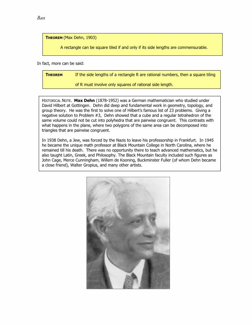
HISTORICAL NOTE. Max Dehn (1878-1952) was a German mathematician who studied under David Hilbert at Gottingen. Dehn did deep and fundamental work in geometry, topology, and group theory. He was the first to solve one of Hilbert’s famous list of 23 problems. Giving a negative solution to Problem #3, Dehn showed that a cube and a regular tetrahedron of the same volume could not be cut into polyhedra that are pairwise congruent. This contrasts with what happens in the plane, where two polygons of the same area can be decomposed into triangles that are pairwise congruent. In 1938 Dehn, a Jew, was forced by the Nazis to leave his professorship in Frankfurt. In 1945 he became the unique math professor at Black Mountain College in North Carolina, where he remained till his death. There was no opportunity there to teach advanced mathematics, but he also taught Latin, Greek, and Philosophy. The Black Mountain faculty included such figures as John Cage, Merce Cunningham, Willem de Kooning, Buckminster Fuller (of whom Dehn became a close friend), Walter Gropius, and many other artists.

THEOREM If the side lengths of a rectangle R are rational numbers, then a square tiling of R must involve only squares of rational side length.

TMME, vol8, nos.1&2, p .29

Consulting the literature in pursuit of the questions above was the occasion for learning some very interesting mathematics (old, but much of it new for me), and I welcomed the opportunity to thereby gain new knowledge and techniques, as well as culturally broaden my mathematical horizons. I did not hesitate to take in more than was needed for the questions that motivated my search. I’ll report on some of the highlights below, providing mathematical details only when they are within reach of high school mathematics.

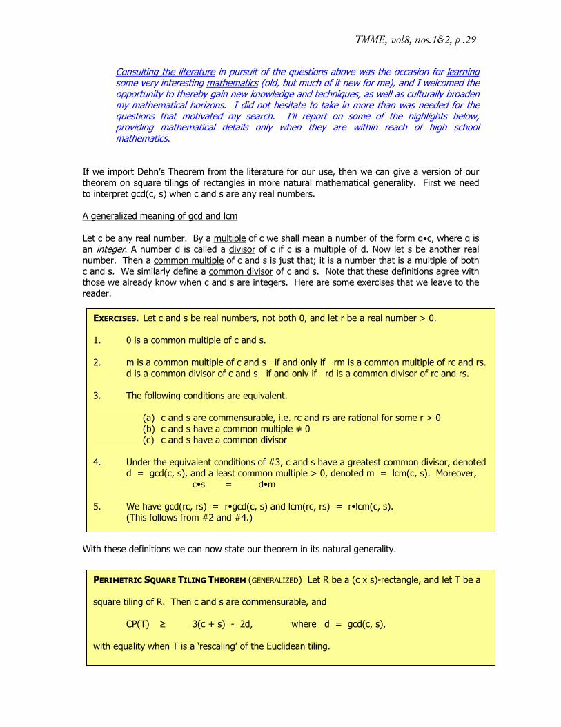
If we import Dehn’s Theorem from the literature for our use, then we can give a version of our theorem on square tilings of rectangles in more natural mathematical generality. First we need to interpret gcd(c, s) when c and s are any real numbers. A generalized meaning of gcd and lcm Let c be any real number. By a multiple of c we shall mean a number of the form q•c, where q is an integer. A number d is called a divisor of c if c is a multiple of d. Now let s be another real number. Then a common multiple of c and s is just that; it is a number that is a multiple of both c and s. We similarly define a common divisor of c and s. Note that these definitions agree with those we already know when c and s are integers. Here are some exercises that we leave to the reader.

With these definitions we can now state our theorem in its natural generality.

EXERCISES. Let c and s be real numbers, not both 0, and let r be a real number > 0. 1. 0 is a common multiple of c and s. 2. m is a common multiple of c and s if and only if rm is a common multiple of rc and rs.

d is a common divisor of c and s if and only if rd is a common divisor of rc and rs. 3. The following conditions are equivalent.

(a) c and s are commensurable, i.e. rc and rs are rational for some r > 0 (b) c and s have a common multiple ≠ 0 (c) c and s have a common divisor

4. Under the equivalent conditions of #3, c and s have a greatest common divisor, denoted

d = gcd(c, s), and a least common multiple > 0, denoted m = lcm(c, s). Moreover, c•s = d•m

5. We have gcd(rc, rs) = r•gcd(c, s) and lcm(rc, rs) = r•lcm(c, s). (This follows from #2 and #4.)

PERIMETRIC SQUARE TILING THEOREM (GENERALIZED) Let R be a (c x s)-rectangle, and let T be a square tiling of R. Then c and s are commensurable, and CP(T) ≥ 3(c + s) - 2d, where d = gcd(c, s), with equality when T is a ‘rescaling’ of the Euclidean tiling.

Bass

The discussion above was designed just to give meaning to the quantity “gcd(c, s)” in the theorem. The definitions and exercises are a fairly typical example of how a mathematician may try to find a natural general framework for some mathematical concept. With some elementary concepts from “group theory” (out of bounds in the present discussion) one could give a more conceptual and more precise formulation to these ideas.

The proof of the Generalized Perimetric Square Tiling Theorem goes as follows. The commensurability of c and s is just Dehn’s Theorem. So, after rescaling R and T, we can assume that c and s are rational. Then the sequel to Dehn’s theorem tells us further that the tiles in T all have rational side length as well. Choosing a common denominator for c and s and all the side lengths of tiles in T, we can use this to rescale the situation again and arrange that c and s are integers, as are the side lengths of all the tiles in T. Now we are in a position to quote the Perimetric Square Tiling Theorem we proved above under these conditions. Finally, we scale back to the original R and T. Exercise #5 above is used to see that gcd(c, s) behaves consistently in each of these rescalings.

Dehn’s Theorem tells us that square tileable rectangles are commensuarable, i.e. their side lengths are rational after rescaling. A further rescaling makes the side lengths integers, where we can apply the earlier Perimetric Square Tiling Theorem. To scale back to the original rectangle and tiling, we need to know how to give meaning to a rescaling of the gcd(c, s) that appears in the earlier theorem. That is what we worked to accomplish in the discussion preceding the generalized theorem. So finding the “mathematical boundary” of our result had two ingredients. First, Dehn’s Theorem restricts the geometric boundary of the set of rectangles for which it is meaningful to discuss square tilings. Second, we conceptually expanded the algebraic notion of gcd(c, s) so that it has meaning in the full geometric context defined by Dehn’s Theorem.

The only ‘gap’ in our story now, i.e. the only component that we have not mathematically derived from essentially High School level mathematics, is Dehn’s Theorem itself. Can we make that also accessible?

Proofs of Dehn’s Theorem There are several proofs of Dehn’s Theorem, but I have not found one that stays within the mathematical bounds that I have tried to maintain here. Dehn’s original proof (Dehn, 1903) was quite complicated. Later proofs (see for example, Freiling and Rinne, 1994) are short and elegant, but make use of some abstract linear algebra, and the Axiom of Choice. An ingenious proof was devised by Brooks et al, (1940). From a square tiling of a rectangle, they constructed an electrical circuit, and used Kirchoff’s Laws to deduce Dehn’s Theorem, as well as many interesting generalizations. This method is also described in Blackett’s book on Elementary Topology (1982). For mathematical completeness, but outside the framework of the exposition above, we provide here a proof of Dehn’s Theorem as used here. First a preliminary on “area functions.”

TMME, vol8, nos.1&2, p .31

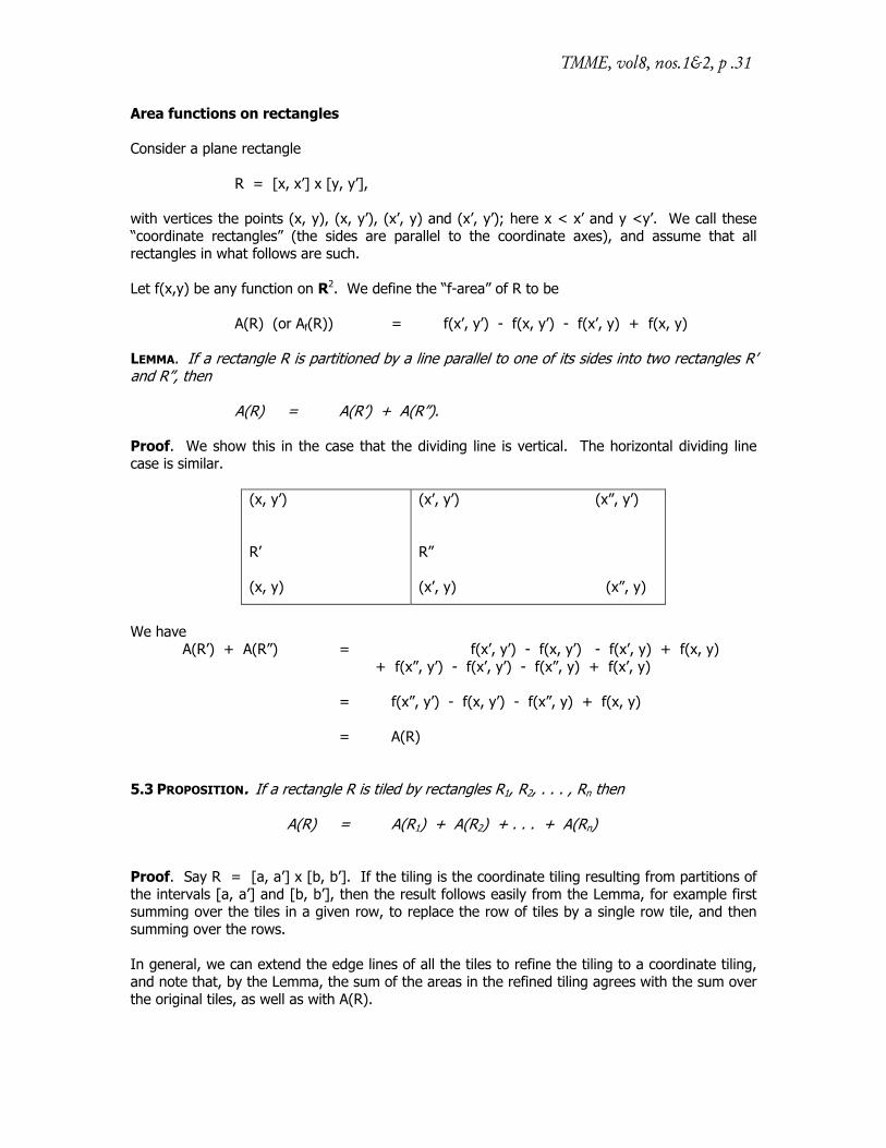
Area functions on rectangles Consider a plane rectangle R = [x, x’] x [y, y’], with vertices the points (x, y), (x, y’), (x’, y) and (x’, y’); here x < x’ and y <y’. We call these “coordinate rectangles” (the sides are parallel to the coordinate axes), and assume that all rectangles in what follows are such. Let f(x,y) be any function on R2. We define the “f-area” of R to be A(R) (or Af(R)) = f(x’, y’) - f(x, y’) - f(x’, y) + f(x, y) LEMMA. If a rectangle R is partitioned by a line parallel to one of its sides into two rectangles R’ and R”, then A(R) = A(R’) + A(R”). Proof. We show this in the case that the dividing line is vertical. The horizontal dividing line case is similar.

(x, y’) R’ (x, y)

(x’, y’) (x”, y’) R” (x’, y) (x”, y)

We have A(R’) + A(R”) = f(x’, y’) - f(x, y’) - f(x’, y) + f(x, y) + f(x”, y’) - f(x’, y’) - f(x”, y) + f(x’, y) = f(x”, y’) - f(x, y’) - f(x”, y) + f(x, y) = A(R) 5.3 PROPOSITION. If a rectangle R is tiled by rectangles R1, R2, . . . , Rn then A(R) = A(R1) + A(R2) + . . . + A(Rn) Proof. Say R = [a, a’] x [b, b’]. If the tiling is the coordinate tiling resulting from partitions of the intervals [a, a’] and [b, b’], then the result follows easily from the Lemma, for example first summing over the tiles in a given row, to replace the row of tiles by a single row tile, and then summing over the rows. In general, we can extend the edge lines of all the tiles to refine the tiling to a coordinate tiling, and note that, by the Lemma, the sum of the areas in the refined tiling agrees with the sum over the original tiles, as well as with A(R).

Bass

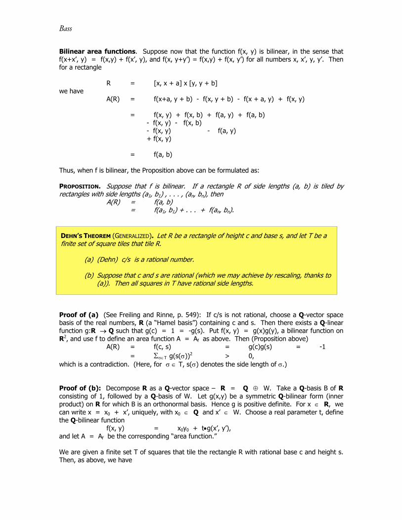
Bilinear area functions. Suppose now that the function f(x, y) is bilinear, in the sense that f(x+x’, y) = f(x,y) + f(x’, y), and f(x, y+y’) = f(x,y) + f(x, y’) for all numbers x, x’, y, y’. Then for a rectangle R = [x, x + a] x [y, y + b] we have A(R) = f(x+a, y + b) - f(x, y + b) - f(x + a, y) + f(x, y) = f(x, y) + f(x, b) + f(a, y) + f(a, b) - f(x, y) - f(x, b) - f(x, y) - f(a, y) + f(x, y) = f(a, b) Thus, when f is bilinear, the Proposition above can be formulated as: PROPOSITION. Suppose that f is bilinear. If a rectangle R of side lengths (a, b) is tiled by rectangles with side lengths (a1, b1) , . . . , (an, bn), then A(R) = f(a, b) = f(a1, b1) + . . . + f(an, bn).

Proof of (a) (See Freiling and Rinne, p. 549): If c/s is not rational, choose a Q-vector space basis of the real numbers, R (a “Hamel basis”) containing c and s. Then there exists a Q-linear function g:R Q such that g(c) = 1 = -g(s). Put f(x, y) = g(x)g(y), a bilinear function on R2, and use f to define an area function A = Af as above. Then (Proposition above)

A(R) = f(c, s) = g(c)g(s) = -1 = T g(s())2 > 0,

which is a contradiction. (Here, for T, s() denotes the side length of .) Proof of (b): Decompose R as a Q-vector space – R = Q W. Take a Q-basis B of R consisting of 1, followed by a Q-basis of W. Let g(x,y) be a symmetric Q-bilinear form (inner product) on R for which B is an orthonormal basis. Hence g is positive definite. For x R, we can write x = x0 + x’, uniquely, with x0 Q and x’ W. Choose a real parameter t, define the Q-bilinear function f(x, y) = x0y0 + tg(x’, y’), and let A = Af be the corresponding “area function.” We are given a finite set T of squares that tile the rectangle R with rational base c and height s. Then, as above, we have

DEHN’S THEOREM (GENERALIZED). Let R be a rectangle of height c and base s, and let T be a finite set of square tiles that tile R.

(a) (Dehn) c/s is a rational number. (b) Suppose that c and s are rational (which we may achieve by rescaling, thanks to

(a)). Then all squares in T have rational side lengths.

TMME, vol8, nos.1&2, p .33

A(R) = f(c, s) = cs > 0 = T f(s(),s()) = 1≤i≤r f(s(i),s(i)),

where s(1), s(2), . . . , s(r) is the list of side lengths of the square tiles in T. We can write s(i) = s(i)0 + s(i)’, with s(i)0 Q and s(i)’ W. Then f(s(i), s(i)) = s(i)0

2 + tg(s(i)’, s(i)’) These f(s(i), s(i)) are linear functions of t, with t-coefficient ≥ 0, and > 0 if s(i) is irrational. Since their sum, A(R), is a constant (independent of t) it follows that none of the s(i) can be irrational.

IV. CONCLUSION I have tried to provide a vivid image of a small piece of ‘mathematics in the making,’ accessible (apart from this last section on Dehn’s Theorem) with only a base of High School level mathematics. The main agenda, carried by the interleaved meta-discussion, was to make explicit some of the moves, dispositions, and motivations that guided the mathematical work. My hope is that this can help illuminate some of the resources that mathematicians deploy in the course of their work, and that many of these will resonate with and prove helpful to teachers and learners of school mathematics.

V. REFERENCES

Blackett, D. W. (1982). Elementary Topology: A Combinatorial and Algebraic Approach, Academic Press, New York. Brooks, R. L., Smith, C. A. B., Stone, A. H., and Tutte, W. T. (1940). The Dissection of Rectangles into Squares, Duke Mathematics Journal, 7, 312-340 Cuoco, A., Goldenberg, E. P., and Mark, J. (2007). Habits of Mind (in preparation, for the Connected Geometry curriculum, Educational Development Center, Newton, MA) Davis, P. J. and Hersh, R. (1981). The Mathematical Experience, Birkhauser Boston. Dehn, Max (1903). Über die Zerlegung von Rechtecken in Rechtecke, Mathematische Annalen, 57, 314-332. Freiling, C. and Rinne, D. (1994). Tiling a square with similar rectangles, Mathematical Research Letters, 1, 547-558 Hadamard, J. (1973). The Mathematician’s Mind: The Psychology of Invention in the Mathematical Field, Princeton University Press. Originally published (1945) as, The Psychology of Invention in the Mathematical Field, Princeton University Press. Kenyon, R. (1994). Tiling a rectangle with the fewest squares, arXiv:math.CO/9411215 v1, 28 Nov 1994

Bass

Lakatos, Imre (1976). Proofs and Refutations, Cambridge University Press. National Council of Teachers of Mathematics (2000). Principles and Standards for School Mathematics. Poincaré, H. (2003) Science and Method, Dover, New York. Translated from Science et Méthode, (1908), Flammarion, Paris. Polya, G. (1954), Mathematics and Plausible Reasoning, Vols. I & II, Princeton University Press. Stein, S. K. (1999). Mathematics: The Man-Made Universe, Dover Pubilications, Inc. New York