Embed Size (px)
Citation preview

Viola 2003
Learning and Vision:Discriminative Models
Chris Bishop and Paul Viola

Viola 2003
Part II: Algorithms and Applications
• Part I: Fundamentals
• Part II: Algorithms and Applications
• Support Vector Machines– Face and pedestrian detection
• AdaBoost– Faces
• Building Fast Classifiers– Trading off speed for accuracy…
– Face and object detection
• Memory Based Learning– Simard
– Moghaddam

Viola 2003
History Lesson• 1950’s Perceptrons are cool
– Very simple learning rule, can learn “complex” concepts
– Generalized perceptrons are better -- too many weights
• 1960’s Perceptron’s stink (M+P)– Some simple concepts require exponential # of features
• Can’t possibly learn that, right?
• 1980’s MLP’s are cool (R+M / PDP)– Sort of simple learning rule, can learn anything (?)
– Create just the features you need
• 1990 MLP’s stink– Hard to train : Slow / Local Minima
• 1996 Perceptron’s are cool

Viola 2003
Why did we need multi-layer perceptrons?
• Problems like this seem to require very complex non-linearities.
• Minsky and Papert showed that an exponential number of features is necessary to solve generic problems.

Viola 2003
Why an exponential number of features?
...,,,,,
,,,,,
,,,
,,
,
1
)(
52
421
32
21
22
312
41
51
42
321
22
21
22
212
31
41
32
22
11
12
21
31
22
12
11
21
12
11
xxxxxxxxxx
xxxxxxxxxx
xxxxxx
xxxx
xx
x
14th Order???120 Features
),min(!!
)!( nk knOnk
kn
k
kn
),min(!!
)!( nk knOnk
kn
k
kn
polyorder :
variables:
k
npolyorder :
variables:
k
n
N=21, k=5 --> 65,000 featuresN=21, k=5 --> 65,000 features

Viola 2003
MLP’s vs. Perceptron
• MLP’s are hard to train… – Takes a long time (unpredictably long)
– Can converge to poor minima
• MLP are hard to understand– What are they really doing?
• Perceptrons are easy to train… – Type of linear programming. Polynomial time.
– One minimum which is global.
• Generalized perceptrons are easier to understand.– Polynomial functions.

Viola 2003
Perceptron Training is Linear Programming
0: iT
i wyi x
Polynomial time in the number of variablesand in the number of constraints.
isi 0
i
ismin
What about linearly inseparable?
0: iiT
i swyi x
),(
:
}1,1{:
ii
N
y
R
y
x
x
),(
:
}1,1{:
ii
N
y
R
y
x
x

Viola 2003
Rebirth of Perceptrons
• How to train effectively– Linear Programming (… later quadratic programming)
– Though on-line works great too.
• How to get so many features inexpensively?!?– Kernel Trick
• How to generalize with so many features?– VC dimension. (Or is it regularization?)
Support Vector Machines

Viola 2003
Lemma 1: Weight vectors are simple
• The weight vector lives in a sub-space spanned by the examples… – Dimensionality is determined by the number of
examples not the complexity of the space.
xw00 w
l
llt
tt bw xx
l
llbw )(x

Viola 2003
Lemma 2: Only need to compare examples
lll
l
Tll
T
lll
T
Kb
b
b
wy
),(
)()(
)()(
)()(
xx
xx
xx
xx l
llbw )(x

Viola 2003
Simple Kernels yield Complex Features
22112
222
21
21
22211
2
21
)1(
)1(),(
xxxxxxxx
xxxx
K T
xxxx
21
22
21
1
)(
xx
x
xx

Viola 2003
But Kernel Perceptrons CanGeneralize Poorly
14)1(),( xxxx TK

Viola 2003
Perceptron Rebirth: Generalization• Too many features … Occam is unhappy
– Perhaps we should encourage smoothness?
0),(: iij
jji sKbyi xx
0: isi
i
ismin
j
jb2min
Smoother

Viola 2003
The linear program can return any multiple of the correct weight vector...
Linear Program is not unique
Slack variables & Weight prior - Force the solution toward zero
0: iT
i wyi x 0: iT
i wyi x
iswy iiT
i 0x
isi 0
i
ismin
wwTmin

Viola 2003
Definition of the Margin
• Geometric Margin: Gap between negatives and positives measured perpendicular to a hyperplane
• Classifier Margin iT
NEGii
T
POSiww xx
maxmin

Viola 2003
Require non-zero margin
Allows solutionswith zero margin
lsw llT 1x
Enforces a non-zeromargin between examplesand the decision boundary.
lsw llT 0x

Viola 2003
Constrained Optimization
• Find the smoothest function that separates data– Quadratic Programming (similar to Linear
Programming)• Single Minima
• Polynomial Time algorithm
1),( llj
jjl sKby xx
0ls
l
lsmin
j
jb2min
Viola 2003
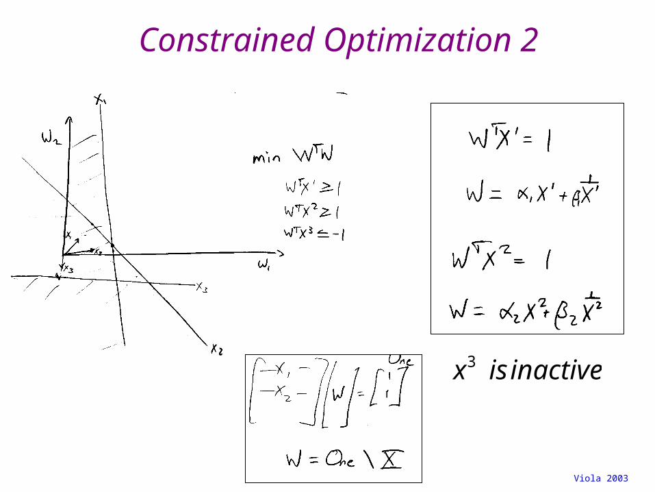
Constrained Optimization 2
inactiveisx3

Viola 2003
SVM: examples

Viola 2003
SVM: Key Ideas
• Augment inputs with a very large feature set– Polynomials, etc.
• Use Kernel Trick(TM) to do this efficiently• Enforce/Encourage Smoothness with weight penalty• Introduce Margin• Find best solution using Quadratic Programming

Viola 2003
SVM: Zip Code recognition
• Data dimension: 256• Feature Space: 4 th order
– roughly 100,000,000 dims

Viola 2003
The Classical Face Detection Process
SmallestScale
LargerScale
50,000 Locations/Scales

Viola 2003
Classifier is Learned from Labeled Data
• Training Data– 5000 faces
• All frontal
– 108 non faces
– Faces are normalized• Scale, translation
• Many variations– Across individuals
– Illumination
– Pose (rotation both in plane and out)

Viola 2003
Key Properties of Face Detection
• Each image contains 10 - 50 thousand locs/scales• Faces are rare 0 - 50 per image
– 1000 times as many non-faces as faces
• Extremely small # of false positives: 10-6

Viola 2003
Sung and Poggio

Viola 2003
Rowley, Baluja & Kanade
First Fast System - Low Res to Hi

Viola 2003
Osuna, Freund, and Girosi

Viola 2003
Support Vectors

Viola 2003
P, O, & G: First Pedestrian Work

Viola 2003
On to AdaBoost
• Given a set of weak classifiers
– None much better than random
• Iteratively combine classifiers– Form a linear combination
– Training error converges to 0 quickly
– Test error is related to training margin
}1,1{)( :originally xjh
rated" confidence" },{)( also xjh
t
t bxhxC )()(

Viola 2003
AdaBoostWeak
Classifier 1
WeightsIncreased
Weak classifier 3
Final classifier is linear combination of weak classifiers
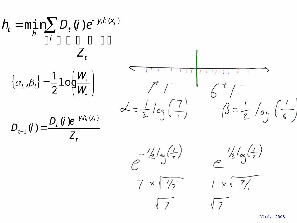
W
Wtt log
2
1,
t
xhyt
t Z
eiDiD
iti )(
1
)()(
t
i
xhyt
ht
Z
eiDh ii )()(min
Weak Classifier 2
Freund & Shapire

Viola 2003
AdaBoost Properties
i
xhy
tt
titi
eZ)(
i
ii xCyLoss )(,
t
xhyt
t Z
eiDiD
iti )(
1
)()(
tt
t
xhy
Z
e iti )(
tt
xhy
Z
e titi )(
i
xhy
tt
titi
eZ)(
)(,)(
ii
xhy
xCyLosse titi

Viola 2003
AdaBoost: Super Efficient Feature Selector
• Features = Weak Classifiers
• Each round selects the optimal feature given:– Previous selected features– Exponential Loss

Viola 2003
Boosted Face Detection: Image Features
“Rectangle filters”
Similar to Haar wavelets Papageorgiou, et al.
000,000,6100000,60 Unique Binary Features
otherwise
)( if )(
t
tittit
xfxh
t
t bxhxC )()(

Viola 2003
Viola 2003
W
Wtt log
2
1,
t
xhyt
t Z
eiDiD
iti )(
1
)()(
t
i
xhyt
ht
Z
eiDh ii )()(min

Viola 2003
Feature Selection
• For each round of boosting:– Evaluate each rectangle filter on each example
– Sort examples by filter values
– Select best threshold for each filter (min Z)
– Select best filter/threshold (= Feature)
– Reweight examples
• M filters, T thresholds, N examples, L learning time
– O( MT L(MTN) ) Naïve Wrapper Method
– O( MN ) Adaboost feature selector

Viola 2003
Example Classifier for Face Detection
ROC curve for 200 feature classifier
A classifier with 200 rectangle features was learned using AdaBoost
95% correct detection on test set with 1 in 14084false positives.
Not quite competitive...

Viola 2003
Building Fast Classifiers
• Given a nested set of classifier hypothesis classes
• Computational Risk Minimization
vs false neg determined by
% False Pos
% D
etec
tion
0 50
50
100
FACEIMAGESUB-WINDOW
Classifier 1
F
T
NON-FACE
Classifier 3T
F
NON-FACE
F
T
NON-FACE
Classifier 2T
F
NON-FACE

Viola 2003
Other Fast Classification Work
• Simard
• Rowley (Faces)• Fleuret & Geman (Faces)

Viola 2003
Cascaded Classifier
1 Feature 5 Features
F
50%20 Features
20% 2%
FACE
NON-FACE
F
NON-FACE
F
NON-FACE
IMAGESUB-WINDOW
• A 1 feature classifier achieves 100% detection rate and about 50% false positive rate.
• A 5 feature classifier achieves 100% detection rate and 40% false positive rate (20% cumulative)– using data from previous stage.
• A 20 feature classifier achieve 100% detection rate with 10% false positive rate (2% cumulative)

Viola 2003
Comparison to Other Systems
(94.8)Roth-Yang-Ahuja
94.4Schneiderman-Kanade
89.990.189.286.083.2Rowley-Baluja-Kanade
93.791.891.190.890.190.088.885.278.3Viola-Jones
422167110957865503110Detector
False Detections

Viola 2003
Output of Face Detector on Test Images

Viola 2003
Solving other “Face” Tasks
Facial Feature Localization
DemographicAnalysis
Profile Detection

Viola 2003
Feature Localization
• Surprising properties of our framework– The cost of detection is not a function of image size
• Just the number of features
– Learning automatically focuses attention on key regions
• Conclusion: the “feature” detector can include a large contextual region around the feature

Viola 2003
Feature Localization Features
• Learned features reflect the task

Viola 2003
Profile Detection

Viola 2003
More Results

Viola 2003
Profile Features

Viola 2003
One-Nearest Neighbor…One nearest neighbor for fitting is described shortly…
Similar to Join The Dots with two Pros and one Con.
• PRO: It is easy to implement with multivariate inputs.
• CON: It no longer interpolates locally.
• PRO: An excellent introduction to instance-based learning…
Thanks toAndrew Moore

Viola 2003
1-Nearest Neighbor is an example of…. Instance-based learning
Four things make a memory based learner:• A distance metric• How many nearby neighbors to look at?• A weighting function (optional)• How to fit with the local points?
x1 y1
x2 y2
x3 y3
.
.xn yn
A function approximator that has been around since about 1910.
To make a prediction, search database for similar datapoints, and fit with the local points.
Thanks toAndrew Moore

Viola 2003
Nearest Neighbor
Four things make a memory based learner:
1. A distance metricEuclidian
2. How many nearby neighbors to look at?One
3. A weighting function (optional)Unused
4. How to fit with the local points?Just predict the same output as the nearest
neighbor.
Thanks toAndrew Moore

Viola 2003
Multivariate Distance Metrics
Suppose the input vectors x1, x2, …xn are two dimensional:
x1 = ( x11 , x12 ) , x2 = ( x21 , x22 ) , …xN = ( xN1 , xN2 ).
One can draw the nearest-neighbor regions in input space.
Dist(xi,xj) = (xi1 – xj1)2 + (xi2 – xj2)2 Dist(xi,xj) =(xi1 – xj1)2+(3xi2 – 3xj2)2
The relative scalings in the distance metric affect region shapes.
Thanks toAndrew Moore

Viola 2003
Euclidean Distance Metric
Other Metrics…
• Mahalanobis, Rank-based, Correlation-based (Stanfill+Waltz, Maes’ Ringo system…)
2N
22
21
22
σ00
0σ0
00σ
)x'-(x)x'-(x )x'(x,
' )x'(x,
T
iiii
D
xxD
where
Or equivalently,
Thanks toAndrew Moore

Viola 2003
Notable Distance MetricsThanks toAndrew Moore

Viola 2003
Simard: Tangent Distance

Viola 2003
Simard: Tangent Distance

Viola 2003
FERET Photobook Moghaddam & Pentland (1995)
Thanks toBaback Moghaddam

Viola 2003
Eigenfaces Moghaddam & Pentland (1995)
Normalized Eigenfaces
Thanks toBaback Moghaddam

Viola 2003
Euclidean (Standard) “Eigenfaces” Turk & Pentland (1992) Moghaddam & Pentland (1995)
Projects all the training facesonto a universal eigenspace to “encode” variations (“modes”)via principal components (PCA)
Uses inverse-distanceas a similarity measurefor matching & recognition
U
Thanks toBaback Moghaddam

Viola 2003
• Metric (distance-based) Similarity Measures
– template-matching, normalized correlation, etc
• Disadvantages
– Assumes isotropic variation (that all variations are equi-probable)
– Can not distinguish incidental changes from the critical ones
– Particularly bad for Face Recognition in which so many are incidental!
• for example: lighting and expression
Euclidean Similarity Measures
k
jiji xxxxS
),(
Thanks toBaback Moghaddam

Viola 2003
PCA-Based Density Estimation Moghaddam & Pentland ICCV’95
Perform PCA and factorize into (orthogonal)Gaussians subspaces:
See Tipping & Bishop (97) for an ML derivation within a more general factor analysis framework (PPCA)
Solve for minimal KL divergence residual for the orthogonal subspace:
Thanks toBaback Moghaddam

Viola 2003
Bayesian Face Recognition Moghaddam et al ICPR’96, FG’98, NIPS’99, ICCV’99
)}()(:{I jiji xLxLxx
)}()(:{E jiji xLxLxx
)|( PMoghaddam ICCV’95 PCA-based density estimation
Intrapersonal Extrapersonal
I
Edual subspaces for
dyads (image pairs)
)()|()()|(
)()|()(
EEII
II
PPPP
PPS
Equate “similarity” with posterior on I
Thanks toBaback Moghaddam

Viola 2003
Intra-Extra (Dual) Subspaces
specs specslight mouthsmile smile smile smile
Intra
Extra
StandardPCA
Thanks toBaback Moghaddam

Viola 2003
Intra-Extra Subspace Geometry
Two “pancake” subspaces with different orientations intersecting near the origin. If each is in fact Gaussian, then the optimal discriminant is hyperquadratic
)φφ(cos 1E
1I
1
Thanks toBaback Moghaddam

Viola 2003
• Bayesian (MAP) Similarity
– priors can be adjusted to reflect operational settings or used for Bayesian fusion
(evidential “belief” from another level of inference)
• Likelihood (ML) Similarity
Bayesian Similarity Measure
)|()( I PSML
Intra-only (ML) recognition is only slightly inferior to MAP (by few %). Therefore, if you had to pick only one subspace to work in, you should pick Intra – and not standard eigenfaces!
1
II
EE
)()|(
)()|(1)(
PP
PPSMAP
Thanks toBaback Moghaddam

Viola 2003
FERET Identification: Pre-Test
Bayesian (Intra-Extra) Standard (Eigenfaces)
Thanks toBaback Moghaddam

Viola 2003
Official 1996 FERET Test
Bayesian (Intra-Extra) Standard (Eigenfaces)
Thanks toBaback Moghaddam

Viola 2003
One-Nearest Neighbor
Objection:
That noise-fitting is really objectionable.
What’s the most obvious way of dealing with it?
..let’s leave distance metrics for now, and go back to….Thanks toAndrew Moore

Viola 2003
k-Nearest Neighbor
Four things make a memory based learner:
1. A distance metricEuclidian
2. How many nearby neighbors to look at? k
3. A weighting function (optional)Unused
4. How to fit with the local points? Just predict the average output among the k nearest neighbors.
Thanks toAndrew Moore

Viola 2003
k-Nearest Neighbor (here k=9)
K-nearest neighbor for function fitting smoothes away noise, but there are clear deficiencies.
What can we do about all the discontinuities that k-NN gives us?
A magnificent job of noise-smoothing. Three cheers for 9-nearest-neighbor.But the lack of gradients and the jerkiness isn’t good.
Appalling behavior! Loses all the detail that join-the-dots and 1-nearest-neighbor gave us, yet smears the ends.
Fits much less of the noise, captures trends. But still, frankly, pathetic compared with linear regression.
Thanks toAndrew Moore

Viola 2003
Kernel Regression
Four things make a memory based learner:
1. A distance metricScaled Euclidian
2. How many nearby neighbors to look at? All of them
3. A weighting function (optional) wi = exp(-D(xi, query)2 / Kw
2)
Nearby points to the query are weighted strongly, far points weakly. The KW parameter is the Kernel Width. Very important.
4. How to fit with the local points?Predict the weighted average of the outputs:
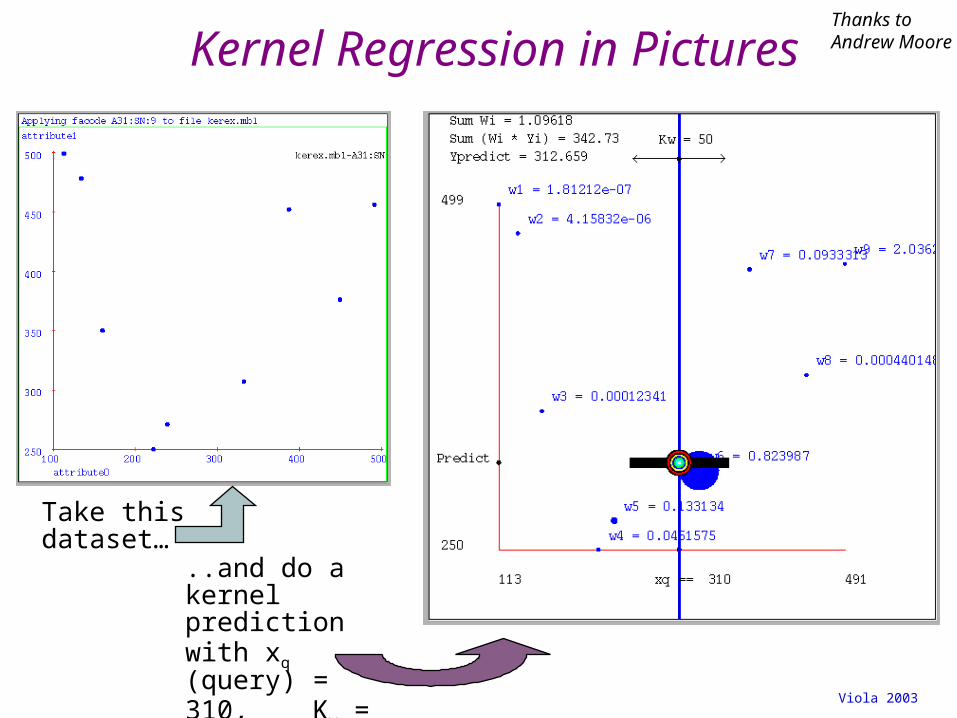
predict = Σwiyi / Σwi
Thanks toAndrew Moore
Viola 2003
Kernel Regression in Pictures
Take this dataset…
..and do a kernel prediction with xq (query) = 310, Kw = 50.
Thanks toAndrew Moore

Viola 2003
Varying the Query
xq = 150 xq = 395
Thanks toAndrew Moore

Viola 2003
Varying the kernel width
Increasing the kernel width Kw means further away points get an opportunity to influence you.
As Kwinfinity, the prediction tends to the global average.
xq = 310
KW = 50 (see the double arrow at top of diagram)
xq = 310 (the same)
KW = 100
xq = 310 (the same)
KW = 150
Thanks toAndrew Moore

Viola 2003
Kernel Regression Predictions
Increasing the kernel width Kw means further away points get an opportunity to influence you.
As Kwinfinity, the prediction tends to the global average.
KW=10 KW=20 KW=80
Thanks toAndrew Moore

Viola 2003
Kernel Regression on our test cases
KW=1/32 of x-axis width.
It’s nice to see a smooth curve at last. But rather bumpy. If Kw gets any higher, the fit is poor.
KW=1/32 of x-axis width.
Quite splendid. Well done, kernel regression. The author needed to choose the right KW to achieve this.
KW=1/16 axis width.
Nice and smooth, but are the bumps justified, or is this overfitting?
Choosing a good Kw is important. Not just for Kernel Regression, but for all the locally weighted learners we’re about to see.
Thanks toAndrew Moore
Viola 2003
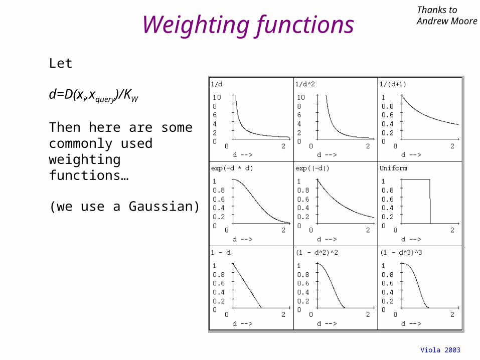
Weighting functions
Let
d=D(xi,xquery)/KW
Then here are some commonly used weighting functions…
(we use a Gaussian)
Thanks toAndrew Moore

Viola 2003
Kernel Regression can look bad
KW = Best.
Clearly not capturing the simple structure of the data.. Note the complete failure to extrapolate at edges.
KW = Best.
Also much too local. Why wouldn’t increasing Kw help? Because then it would all be “smeared”.
KW = Best.
Three noisy linear segments. But best kernel regression gives poor gradients.
Time to try something more powerful…
Thanks toAndrew Moore

Viola 2003
Locally Weighted Regression
Kernel Regression:Take a very very conservative function approximator called AVERAGING. Locally weight it.
Locally Weighted Regression:Take a conservative function approximator called LINEAR REGRESSION. Locally weight it.
Let’s Review Linear Regression….
Thanks toAndrew Moore

Viola 2003
Unweighted Linear Regression
You’re lying asleep in bed. Then Nature wakes you.
YOU: “Oh. Hello, Nature!”
NATURE: “I have a coefficient β in mind. I took a bunch of real numbers called x1, x2 ..xN thus: x1=3.1,x2=2, …xN=4.5.
For each of them (k=1,2,..N), I generated yk= βxk+εk
where εk is a Gaussian (i.e. Normal) random variable with mean 0 and standard deviation σ. The εk’s were generated independently of each other.
Here are the resulting yi’s: y1=5.1 , y2=4.2 , …yN=10.2”
You: “Uh-huh.”
Nature: “So what do you reckon β is then, eh?”
WHAT IS YOUR RESPONSE?
Thanks toAndrew Moore

Viola 2003
Locally Weighted Regression
Four things make a memory-based learner:1. A distance metric
Scaled Euclidian2. How many nearby neighbors to look at?
All of them3. A weighting function (optional)
wk = exp(-D(xk, xquery)2 / Kw2)
Nearby points to the query are weighted strongly, far points weakly. The Kw parameter is the Kernel Width.
4. How to fit with the local points?1. First form a local linear model. Find the β that minimizes the locally weighted sum of squared
residuals:
2
1
2
β
xβyβ argmin
N
kk
Tkkw
Then predict ypredict=βT xquery
Thanks toAndrew Moore

Viola 2003
How LWR works
Linear regression not flexible but trains like lightning.
Locally weighted regression is very flexible and fast to train.
Query
Thanks toAndrew Moore

Viola 2003
LWR on our test cases
KW = 1/16 of x-axis width. KW = 1/32 of x-axis width. KW = 1/8 of x-axis width.
Nicer and smoother, but even now, are the bumps justified, or is this overfitting?
Thanks toAndrew Moore

Viola 2003
Features, Features, Features
• In almost every case:
Good Features beat Good Learning
Learning beats No Learning
• Critical classifier ratio:
• AdaBoost >> SVM
complexity
quality