Journal of Neuroscience Methods 101 (2000) 117–130

Virtual muscle: a computational approach to understanding theeffects of muscle properties on motor control

Ernest J. Cheng 1, Ian E. Brown, Gerald E. Loeb *Department of Biomedical Engineering, DRB-B12, Medical De6ice De6elopment Facility, Alfred E. Mann Institute for Biomedical Engineering,

Uni6ersity of Southern California, MC 1112, 1042 West 36th Place, Los Angeles, CA 90089-1112, USA

Received 23 August 1999; received in revised form 30 May 2000; accepted 1 June 2000

Abstract

This paper describes a computational approach to modeling the complex mechanical properties of muscles and tendons underphysiological conditions of recruitment and kinematics. It is embodied as a software package for use with Matlab™ and Simulinkthat allows the creation of realistic musculotendon elements for use in motor control simulations. The software employs graphicuser interfaces (GUI) and dynamic data exchange (DDE) to facilitate building custom muscle model blocks and linking them tokinetic analyses of complete musculoskeletal systems. It is scalable in complexity and accuracy. The model is based on recentlypublished data on muscle and tendon properties measured in feline slow- and fast-twitch muscle, and incorporates a novelapproach to simulating recruitment and frequency modulation of different fiber-types in mixed muscles. This software isdistributed freely over the Internet at http://ami.usc.edu/mddf/virtualmuscle. © 2000 Elsevier Science B.V. All rights reserved.

Keywords: Matlab; Simulink; Neurophysiology; Biomechanical modeling; Muscle; Simulation

www.elsevier.com/locate/jneumeth

1. Introduction

The study of motor control seeks to determine howthe central nervous system effects functional, goal-di-rected movement. For conceptual purposes, it is usefulto visualize the mechanisms involved in motor controlas a hierarchy, with the brain at the top, the spinal cordin the middle, and the musculoskeletal plant at thebottom (Loeb et al., 1999). Researchers typically haveattempted to understand the mechanisms of motorcontrol by tackling one level of the hierarchy at a time.For example, the ‘population vector’ paradigm (re-viewed in Georgopoulos, 1986), where directional con-trol of hand movements is correlated with corticalactivity in direction-specific neurons, is concernedmostly with the top level of the hierarchy, the brain.Other theories of motor control have emphasized therole of reflexes at the middle, spinal level of the hier-

archy in setting ‘equilibrium points’ as targets formovements (e.g. Asatryan and Feldman, 1965). How-ever, it has been realized that many discrepancies be-tween the proposed theories and observed behaviormight be explained by the fact that the actual effectorsof movement, the muscles themselves at the lowest levelof the hierarchy, have sophisticated non-linear vis-coelastic properties (Hogan, 1985; Gottlieb, 1996;Karniel and Inbar, 1997; Todorov, 2000).

Recently, increasingly complex models have at-tempted a synthesis of many levels of this hierarchy. Asmore studies use this approach, there is an increasingneed for user-accessible models that accurately describethe behavior of muscle under realistic physiologicalconditions. For example, studies of joint stiffness andstatic and dynamic muscle function based on optimiza-tion criteria are often validated solely with electromyo-grams (EMG; e.g. Kaufman et al., 1991; van der Helm,1994; Osu and Gomi, 1999); with a musculoskeletalmodel, force and impedance could be predicted fromEMG and compared with the results of inverse dy-namic analyses. Other studies have included viscoelasticmuscle elements, but researchers are often required todevelop their own musculotendon models (e.g. Karniel

* Corresponding author. Tel.: +1-213-8211112; fax: +1-213-8211120.

E-mail address: gloeb@usc.edu (G.E. Loeb).1 Present address: Sapient Corporation; 200 West Adams, Ste.

2700, Chicago, IL 60610, USA

0165-0270/00/$ - see front matter © 2000 Elsevier Science B.V. All rights reserved.PII: S0165-0270(00)00258-2

E.J. Cheng et al. / Journal of Neuroscience Methods 101 (2000) 117–130118

and Inbar, 1997; Gonzalez et al., 1997; Soechting andFlanders, 1997); consequently, these models are usuallysimplified and designed with arbitrarily estimatedparameters.

Our goal was to provide a general model of musclethat would be easy-to-use, easily integrated with modelsand simulations of kinetics and control, and at thesame time accurate and scalable in its level of sophisti-cation. This would obviate the need for researchers todevelop their own models of muscle. We integratedseveral recent models of the recruitment of motor units(Brown, 1998), the contractile properties of mammalianmuscle (Brown and Loeb, 2000; Brown et al., 1996b,1999), and the elastic properties of tendon and aponeu-rosis (Scott and Loeb, 1995). We have created a graph-ical user interface (GUI) based software package calledVirtual Muscle that allows researchers who may not beinterested in muscle or motoneuron physiology per seto generate musculotendon simulation ‘blocks’ that canbe used readily with their existing simulations. This isfacilitated by building the model from normalizedparameters (Zajac, 1989) that are readily scaled to themorphometry of specific muscles. For the majority ofusers who need only functional musculotendon ele-ments that accurately reflect the non-linear viscoelasticbehavior of muscle, we have provided data on mam-malian muscle fiber types that can be combined withthe commonly available morphometry of specific mus-

cles (for a summary, see Yamaguchi et al., 1990). Formore ambitious users, entirely new fiber types can becreated, with user-specified properties and recruitmentpatterns.

2. Software/hardware requirements

The Virtual Muscle modeling package is designed torun on Matlab 5.2 or higher (The Mathworks Inc.,Natick, MA) and also requires the Simulink 2.2 orhigher module for Matlab. While the GUI for specify-ing the parameters for the muscle model runs in Mat-lab, the individual muscle blocks created for use in theactual simulations are stand-alone Simulink blocks. Wechose to develop the muscle model for the Matlab/Sim-ulink combination for several reasons. First, Matlaband Simulink are already widely used in sensorimotorresearch, especially in developing motor control simula-tions and studying neural networks. Second, Matlab isavailable on a wide variety of platforms, including PCcompatibles, Apple Macintosh, and various UNIX-based systems. Third, Simulink’s block-oriented naturemakes it simpler for users to conceptualize the relation-ships between the various equations that comprise themuscle model. Finally, Matlab is capable of interfacingwith a large number of external applications, such askinetic analysis software to model the segmental dy-namics. We have provided a sample implementation ofthis using the dynamic data exchange (DDE) interfacecommon to many Microsoft Windows based applica-tions. The muscle model package will run on anyhardware and under any operating system that is capa-ble of running the required Matlab and Simulinkversions.

3. Design of the muscle model

Virtual Muscle was created for use in the context ofa hierarchical model of motor control. Skeletal dynam-ics comprise the lowest level, and are driven by therealistic muscle properties provided by Virtual Muscleat the middle level (see Fig. 1). At the top level, themuscles can be controlled by any arbitrary set of activa-tion commands, ranging from pre-recorded EMG datato dynamic, feedback-driven reflex models, to high levelsimulations of cortical commands. With the use of twoGUI-based Matlab functions, BuildFiberTypes andBuildMuscles, the user defines the properties of eachfiber type and the morphometry of each musculotendonelement. After the properties of each musculotendonelement have been specified, stand-alone Virtual Muscleblocks for use in SIMULINK can be created andintegrated with the skeletal dynamics and control sys-tems, which are provided by the user.

Fig. 1. The interaction between various levels of a hierarchical modelof neuromusculoskeletal control. The highest level, sensorimotorcontrol, drives the muscle mechanics level, which in turn drives theskeletal dynamics level. Feedback also exists between each level of thehierarchy. Behavior of the muscle mechanics level is computationallymodeled with Virtual Muscle blocks. The fiber- and muscle-specificparameters are specified in the BuildFiberTypes and BuildMusclesfunctions prior to simulation. These two functions are not activeduring the simulation, as indicated by the dashed arrow.

E.J. Cheng et al. / Journal of Neuroscience Methods 101 (2000) 117–130 119

Fig. 2. Recruitment scheme as applied to a hypothetical muscleconsisting of two simulated slow-twitch and two fast-twitch motorunits. As activation increases, motor units are recruited sequentially,first on the basis of the recruitment rank of the fiber-type (slow-twitchfibers have a lower recruitment rank than fast-twitch), and then bythe user-specified order of the motor units. All motor units arerecruited when activation reaches Ur, which is user-specified for eachmuscle. The firing frequency of each motor unit modulates linearlybetween minimal ( fmin) and maximal ( fmax) levels. These levels aredefined separately and expressed as multiples of f0.5 for each fibertype; this allows slow-twitch motor units to operate over a differentrange of actual frequencies than fast-twitch units.

into motor units, each consisting of a motor neuronand the several hundred muscle fibers it controls.Groups of similar motor unit types tend to be recruitedtogether, while different motor unit types tend to berecruited in a fixed order. This allows us to simplify themodel by lumping many motor units into single simu-lated motor units; this is justified by the finding thatcontractile element behavior scales well from the sar-comere level to the whole fiber level and also to thelevel of the entire recruitment group (Zajac, 1989). Inthe simplest case, a musculotendon element can bemodeled as a single motor unit composed of homoge-nous muscle fibers; the activation signal then onlymodulates the firing frequency of this motor unit. Ifmultiple motor units and/or different fiber types areused in each musculotendon element, a single activationinput sequentially recruits the motor units based on twoproperties, first, the recruitment rank of the fiber typefor that motor unit defined in BuildFiberTypes, andthen secondarily, the order determined in the Build-Muscles function. As U increases, more motor units arerecruited until a value called Ur is reached (specified foreach muscle in BuildMuscles). Ur is the point at whichall motor units have been recruited; increases in activa-tion beyond this point result only in frequency modula-tion of motor units. Motor unit recruitment threshold isbased on the cumulative fractional physiological cross-sectional area (PCSA) of all motor units recruited priorto the given motor unit, with range of recruitmentbetween 0 and Ur (Fig. 2).

In the example illustrated in Fig. 2, the first twocompartments are slow-twitch (and are thus recruitedfirst), and the Ur for the muscle is 0.8. Note that whileit appears that both slow- and fast-twitch motor unitshave the same firing frequency range, fmin and fmax aredefined in frequency units of f0.5. The normalizationfactor f0.5 is defined as the stimulus frequency necessaryto produce 50% of maximal, isometric force (Brown etal., 1999) and thus has different values depending onfiber type. For each motor unit, the frequency modu-lates from a predetermined fmin, when the unit is firstrecruited, up to fmax, which occurs at full activation forthe muscle. A linear scaling of firing frequency relativeto EMG has been demonstrated experimentally by Mil-ner-Brown et al. (1973a). A common initial firing fre-quency for motor units of a given fiber type and theirconvergence to type-specific maximal firing frequencyat maximal activation have been demonstrated by DeLuca et al. (1996).

To simplify the model, whole muscles are treated aslinear combinations of pure slow- and fast-twitch mus-cle compartments (Zajac, 1989; Brown et al., 1996b).This muscle model differs from almost all others cur-rently available, which have assumed that the contrac-tile properties of muscle scale linearly with neuralactivation (e.g. Otten, 1987; Durfee and Palmer, 1994;

The main objective guiding the design of this packagewas the need to balance simplicity and accuracy. EachVirtual Muscle musculotendon element requires an acti-vation and a length signal as input and returns force asan output, the minimum number of state variables formost models. We have included the following features,which we hope will meet the needs of most researchers.� A single activation input (e.g. net synaptic drive or

EMG envelope) drives a function which serves torecruit incrementally and modulate the firing rate ofany number of specified motor units, with the userable to specify the recruitment order and frequencyrange (Fig. 2).

� Type-specific contractile elements that produce forceas a function of recruitment, frequency modulation,length and velocity, including viscoelastic elementsfor passive muscle force (Fig. 3).

� Passive elastic elements for series-compliance of ten-dons and aponeuroses.While the behavior of each of these components can

be specified in detail by the user, physiologically realis-tic default values have been provided for recruitmentparameters and for the behavior of commonly modeledmammalian fiber types. Further detail on the design ofthese three components is provided below.

The recruitment model is based on that described byBrown (1998). Physiologically, muscles are organized

E.J. Cheng et al. / Journal of Neuroscience Methods 101 (2000) 117–130120

Shue et al., 1995; Brown et al., 1996b). That assump-tion contradicts experimental data that suggests other-wise (Rack and Westbury, 1969; Balnave and Allen,1996). Briefly, various relationships including force–length, force–velocity, activation rise- and fall-times,sag and yield tend to be qualitatively different in fast-and slow-twitch muscle and/or to depend on the fre-quency of firing of motor units (Rack and Westbury,1969; Scott et al., 1996; Brown, 1998; Brown and Loeb,2000).

The in-series compliance of tendons plus aponeuroseshas also been included in the model (see Scott andLoeb, 1995). Tendon compliance is important becauseit causes the length and velocity of the contractileelement to be out of phase with those of the wholemuscle. For example, in an active muscle with a highratio of tendon-to-contractile element length, a stretchto the whole musculotendon system would only slightlylengthen the contractile-element, with the majority ofthe length change being accommodated by lengtheningof the tendon (Zajac, 1989). In fact, under certain

conditions, the musculotendon element can be length-ening while the contractile element within the muscle isshortening, or vice-versa. This behavior would be mis-represented in tendon-less models, which assume thatcontractile length changes are proportional to pathlength changes. Because tendon and aponeurosis havebeen shown to have similar elastic properties, they havebeen grouped into a single term for each musculoten-don element (Scott and Loeb, 1995). The tendon andthe contractile muscle fiber elements both act on amuscle mass that provides inertial damping to preventcomputational instabilities from arising within the mus-cle model (Loeb et al., 1999).

4. Implementation of muscle model

Zajac (1989) advocated a model that defines theproperties of a generic musculotendon element with asingle set of equations. This approach was based on theassumption that the properties of individual sarcom-

Fig. 3. ‘Screen shots’ of the BuildFiberTypes function showing the actual feline and human fiber type databases provided with Virtual Muscle.Each fiber type is entered into a different column. Modifying the parameters in this window can affect the recruitment behavior, active and passiveforce–length relationships, force–velocity relationships and rise and fall times. We created the human fiber type database by modifying theseparameters, as described in Appendix B. The individual coefficients used in the muscle model (see Fig. 4) can be modified directly for each fibertype in a second window available under this GUI (not shown).

E.J. Cheng et al. / Journal of Neuroscience Methods 101 (2000) 117–130 121

eres, when grouped together, can be scaled to representthe properties of muscle fibers and these, in turn, can begrouped to represent whole muscle properties. The fiveparameters required by Zajac’s equations were L0

M (op-timal fascicle length, the length at which the muscleproduces maximal tetanic isometric force), F0

M (maxi-mal tetanic isometric force), a0 (pennation angle of themuscle fibers at L0

M), tC (time-scaling parameter formaximal muscle shortening velocity and rise and falltimes), and LS

T (tendon slack length). Once these mea-sures had been determined for a given muscle, itsbehavior could be reproduced mathematically.

4.1. Defining muscle fiber types

Virtual Muscle utilizes a similar approach in scalingeach motor unit in the simulation, with the followingmodifications (Brown and Loeb, 2000; Brown et al.,1999). In our model we currently ignore pennationangle. Zajac’s fiber-specific parameter tC has been re-placed with V0.5 (velocity of shortening required toproduce 0.5 F0 at 1.0 L0 during a tetanic stimulus; usedto scale the force–velocity dependencies) and f0.5 (stim-ulus frequency necessary to produce 0.5 F0 at 1.0 L0

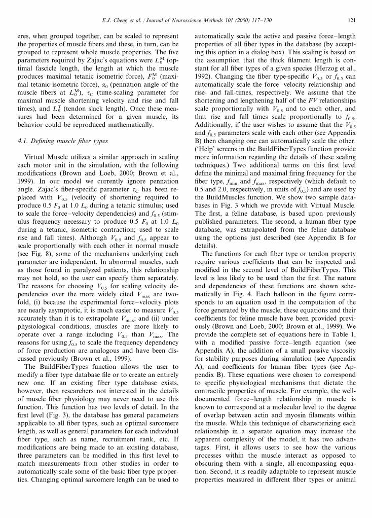
during a tetanic, isometric contraction; used to scalerise and fall times). Although V0.5 and f0.5 appear toscale proportionally with each other in normal muscle(see Fig. 8), some of the mechanisms underlying eachparameter are independent. In abnormal muscles, suchas those found in paralyzed patients, this relationshipmay not hold, so the user can specify them separately.The reasons for choosing V0.5 for scaling velocity de-pendencies over the more widely cited Vmax are two-fold, (i) because the experimental force–velocity plotsare nearly asymptotic, it is much easier to measure V0.5

accurately than it is to extrapolate Vmax; and (ii) underphysiological conditions, muscles are more likely tooperate over a range including V0.5 than Vmax. Thereasons for using f0.5 to scale the frequency dependencyof force production are analogous and have been dis-cussed previously (Brown et al., 1999).

The BuildFiberTypes function allows the user tomodify a fiber type database file or to create an entirelynew one. If an existing fiber type database exists,however, then researchers not interested in the detailsof muscle fiber physiology may never need to use thisfunction. This function has two levels of detail. In thefirst level (Fig. 3), the database has general parametersapplicable to all fiber types, such as optimal sarcomerelength, as well as general parameters for each individualfiber type, such as name, recruitment rank, etc. Ifmodifications are being made to an existing database,three parameters can be modified in this first level tomatch measurements from other studies in order toautomatically scale some of the basic fiber type proper-ties. Changing optimal sarcomere length can be used to

automatically scale the active and passive force–lengthproperties of all fiber types in the database (by accept-ing this option in a dialog box). This scaling is based onthe assumption that the thick filament length is con-stant for all fiber types of a given species (Herzog et al.,1992). Changing the fiber type-specific V0.5 or f0.5 canautomatically scale the force–velocity relationship andrise- and fall-times, respectively. We assume that theshortening and lengthening half of the FV relationshipsscale proportionally with V0.5 and to each other, andthat rise and fall times scale proportionally to f0.5.Additionally, if the user wishes to assume that the V0.5

and f0.5 parameters scale with each other (see AppendixB) then changing one can automatically scale the other.(‘Help’ screens in the BuildFiberTypes function providemore information regarding the details of these scalingtechniques.) Two additional terms on this first leveldefine the minimal and maximal firing frequency for thefiber type, fmin and fmax, respectively (which default to0.5 and 2.0, respectively, in units of f0.5) and are used bythe BuildMuscles function. We show two sample data-bases in Fig. 3 which we provide with Virtual Muscle.The first, a feline database, is based upon previouslypublished parameters. The second, a human fiber typedatabase, was extrapolated from the feline databaseusing the options just described (see Appendix B fordetails).

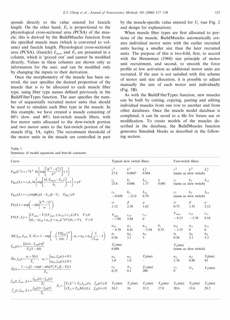
The functions for each fiber type or tendon propertyrequire various coefficients that can be inspected andmodified in the second level of BuildFiberTypes. Thislevel is less likely to be used than the first. The natureand dependencies of these functions are shown sche-matically in Fig. 4. Each balloon in the figure corre-sponds to an equation used in the computation of theforce generated by the muscle; these equations and theircoefficients for feline muscle have been provided previ-ously (Brown and Loeb, 2000; Brown et al., 1999). Weprovide the complete set of equations here in Table 1,with a modified passive force–length equation (seeAppendix A), the addition of a small passive viscosityfor stability purposes during simulation (see AppendixA), and coefficients for human fiber types (see Ap-pendix B). These equations were chosen to correspondto specific physiological mechanisms that dictate thecontractile properties of muscle. For example, the well-documented force–length relationship in muscle isknown to correspond at a molecular level to the degreeof overlap between actin and myosin filaments withinthe muscle. While this technique of characterizing eachrelationship in a separate equation may increase theapparent complexity of the model, it has two advan-tages. First, it allows users to see how the variousprocesses within the muscle interact as opposed toobscuring them with a single, all-encompassing equa-tion. Second, it is readily adaptable to represent muscleproperties measured in different fiber types or animal

E.J. Cheng et al. / Journal of Neuroscience Methods 101 (2000) 117–130122

Fig. 4. Schematic representation of the model equations and terms. These elements were designed to have a one-to-one correspondence with thephysiological substrates of muscle contraction. The behavior of each element is governed by an equation driven by one to four input variables,with one to seven user-modifiable coefficients. The coefficients can be modified in the BuildFiberTypes function. Complete descriptions of theseelements can be found in Brown and Loeb (2000), Brown et al. (1999). FPE1 represents the passive visco-elastic properties of stretching a muscle.FPE2 represents the passive resistance to compression of the thick filaments at short muscle lengths. FL represents the tetanic, isometricforce–length relationship. FV represents the tetanic force–velocity (FV) relationship. Af represents the isometric, activation–frequency (Af )relationship. feff represents the time lag between changes in firing frequency and internal activation (i.e. rise and fall times). Leff represents the timelag between changes in length and the effect of length on the Af relationship. S represents the effects of ‘sag’ on the activation during a constantstimulus frequency. Y represents the effects of yielding (on activation) following movement during sub-maximal activation.

species. It also improves the likelihood that the com-plete model will be reasonably accurate and computa-tionally well-behaved when operated undercombinations of specific morphometry and input condi-tions that were not studied experimentally in the sourcedata.

There are three other ‘global’ properties that affectall the fiber types defined within a single fiber typedatabase. The specific tension, or force per cm2 ofPCSA has been shown to be largely independent ofhistochemical fiber type (Spector et al., 1980; Lucas etal., 1987; Brown et al., 1998); we use 31.8 N cm−2 asan overridable default (Scott et al., 1996; Brown et al.,1998). Specific compliance of series tendon and aponeu-rosis (scaled to PCSA and L0

T) has a nonlinear formbased on feline soleus (Scott and Loeb, 1995). We alsoinclude a passive viscosity for the fascicles with a verysmall default value to provide stability duringsimulations.

Useful functions such as cutting, copying and pastingfiber type parameters along with the underlying coeffi-cients from one column to another are supported. Fibertypes can be imported from one database to another.

4.2. Defining muscle morphometry

The terms required for our modified Zajac-typemodel that are independent of fiber type and are mus-cle-specific are L0, F0, L0

T and Lmax. The first two arethe same as L0

M and F0M defined above and by Zajac

(we drop the ‘M’ so as to not imply muscle, which

many people interpret as including tendon and/oraponeurosis — L0 and F0 are specific to the musclefascicles). L0

T (length of the tendon at maximal tetanicisometric force) replaces Zajac’s tendon slack lengthLS

T. LST is less well defined that L0

T and tends to beabout 5% shorter. Passive tension is based on the newterm Lmax, which is the maximal length of the fasciclesat the maximal anatomical length of the muscle, follow-ing the observation that passive force is more closelycorrelated with Lmax than with L0 (Brown et al., 1996a;see Appendix A for more details). These terms arespecified for each muscle in the second Matlab func-tion, called BuildMuscles. Once these parameters havebeen specified, the user can generate blocks that encap-sulate the behavior of the entire musculotendon ele-ment. The fiber types that comprise the muscles aredrawn from a fiber type database file generated inBuildFiberTypes or pre-supplied by us (we currentlyoffer both feline and human fiber type databases); theBuildMuscles function will not work unless an existingfiber type database file is specified. For each musculo-tendon element to be modeled, the user inputs a singlerow of data into the main BuildMuscles GUI window(Fig. 5A, left). Some data columns are blank andrequire user input. The required morphometric valuesare muscle name, mass, optimal fascicle length, optimaltendon length, and the maximal anatomical musculo-tendon path length. These morphometric measures areeither used directly or converted into the appropriateparameters as required by the set of equations de-scribed previously. For example, the L0 term corre-

E.J. Cheng et al. / Journal of Neuroscience Methods 101 (2000) 117–130 123

sponds directly to the value entered for fasciclelength. On the other hand, F0 is proportional to thephysiological cross-sectional area (PCSA) of the mus-cle; this is derived by the BuildMuscles function fromthe specified muscle mass (which is converted to vol-ume) and fascicle length. Physiological cross-sectionalarea (PCSA), (fascicle) Lmax and F0 are presented in acolumn, which is ‘grayed out’ and cannot be modifieddirectly. Values in these columns are shown only asinformation for the user, and can be modified onlyby changing the inputs to their derivation.

Once the morphometry of the muscle has been en-tered, the user specifies the desired proportion of themuscle that is to be allocated to each muscle fibertype, using fiber type names defined previously in theBuildFiberTypes function. The user specifies the num-ber of sequentially recruited motor units that shouldbe used to simulate each fiber type in the muscle. Inthis example, we have created a muscle consisting of60% slow- and 40% fast-twitch muscle fibers, withfive motor units allocated to the slow-twitch portionand two motor units to the fast-twitch portion of themuscle (Fig. 5A, right). The recruitment threshold ofthe motor units in the muscle are controlled in part

by the muscle-specific value entered for Ur (see Fig. 2and design for explanation).

When muscle fiber types are first allocated to por-tions of the muscle, BuildMuscles automatically cre-ates individual motor units with the earlier recruitedunits having a smaller size than the later recruitedunits. The purpose of this is two-fold, first, to accordwith the Henneman (1968) size principle of motorunit recruitment, and second, to smooth the forceprofile at low activation as additional motor units arerecruited. If the user is not satisfied with this schemeof motor unit size allocation, it is possible to adjustmanually the size of each motor unit individually(Fig. 5B).

As with the BuildFiberTypes function, new musclescan be built by cutting, copying, pasting and editingindividual muscles from one row to another and fromother databases. Once the muscle model database iscompleted, it can be saved to a file for future use ormodification. To create models of the muscles de-scribed in the database, the BuildMuscles functiongenerates Simulink blocks as described in the follow-ing section.

Table 1Summary of model equations and best-fit constants

Typical slow twitch fibersCurve Fast-twitch fibers

kT L rT L r

TcT cT kT

FSE(LT)=cTkT ln!

exp�(LT−L r

T)

kT

n+1

"(same as slow twitch)0.96427.8 0.0047

Lr1 h c1 k2k1 Lr2c1FPE1(L)=c1k1 ln!

exp�(L/Lmax−Lr1)

k1

n+1

"+hV 0.046 1.1723.0 0.001 (same as slow twitch)

Lr2k2c2 Lr2 c2 k2FPE2(L)=c2{exp[k2(L−Lr2)]−1}, FPE250 0.70 (same as slow twitch)−21.0−0.020

v b rrv bFL(L)=exp

�−abs

)LB−1

v

)r�2.121.550.751.621.12 2.30

Vmax cv0 cv1cv1Vmax cv0FV(V, L)=!(Vmax−V)/(Vmax9 (cv0+cv1L)V), V50

(bv−(av0+av1L+av2L2)V)/(bv+V), V\0 9.18−9.15 −5.70−7.88 05.88

av0bvav2av1 av2av0 av1

8.41−4.70 0.35 −1.53 0 0−5.34af nf0 nf1 nf1nf0afAf( feff, Leff, Y, S)=1−exp

�−�YSfeff

afnf

�nfn, nf=nf0+nf1

� 1

Leff

−1�

2.1 3.30.56 52.1 0.56

TL(ms) TL(ms)L: eff(t)=[L(t)−Leff(t)]3

TL(1−Af) 0.088 (same as slow twitch)

as2 TS(ms)as1 as1 TS(ms)as2S: (t, feff)=as−S(t)

Ts

, as=!aS1, feff(t)B0.1

aS2, feff(t)]0.1 1.0 0.961.761.0 – 43

cY TY(ms)VY cY VY TY(ms)Y: (t)=1−cY[1−exp(−abs�V �/VY)]−Y(t)

TY0.35 0.1 0200 ––

Tf3(ms)Tf1(ms) Tf2(ms)Tf4(ms)Tf3(ms)Tf2(ms)Tf1(ms)f: int(t, fenv, L)=

fenv(t)−fint(t)

Tf.,

f:eff

(t, fint, L)=fint(t)−feff(t)

Tf

,Tf=

!Tf1L2+Tf2 fenv(t), f: eff(t)]0

(Tf3+Tf4Af)/(L), f: eff(t)B0 13.61624.2 20.617.8 28.233.2

E.J. Cheng et al. / Journal of Neuroscience Methods 101 (2000) 117–130124

Fig. 5. (A) ‘Screen shot’ of the BuildMuscles function. Parameters for each muscle are modified in this main window. Each muscle is entered intoa separate row. The left-most columns accept muscle morphometry measures for each muscle, while the right-most columns (enclosed by blackframe) describe its composition by fiber-type and numbers of modeled units. (B) Secondary window of BuildMuscles function for displaying andediting fractional PCSA of each motor unit. Motor units of a single fiber type are arranged in columns and recruited sequentially from the topdown.

4.3. Musculotendon blocks

The BuildMuscles function ultimately is used to createSimulink blocks for each muscle you have chosen tomodel, based on the parameters currently entered in theBuildMuscles function and the selected fiber type data-base file. These Simulink blocks are stand-alone and,once created, can run on any supported version ofSimulink, even without the Virtual Muscle packageinstalled. A potential drawback to making the Simulinkblocks stand-alone is that changes made to the databasefiles will not be reflected automatically in the existingblocks. To address this issue, a feature has been includedin the BuildMuscles function that will allow users easilyto replace muscle blocks in existing Simulink model fileswith updated muscle blocks of the same name. Thisfacilitates building a complex simulation and then exam-ining the consequences of making various changes to themuscle properties.

As mentioned previously, the Simulink musculoten-don blocks require inputs for activation, typically be-tween 0 and 1, and for musculotendon path length, incentimeters. In Simulink, these inputs can easily be drivenby constants, ramp or sinusoidal inputs, feedback orfeedforward mechanisms, external data files, or evenoutputs of other software packages. The latter drivingmechanism is explained in a following section. Theoutput from the musculotendon element is force inNewtons. This force output can be used as inputs to otherSimulink blocks, directed to output files or displayscopes, or directed to external applications.

5. Application

5.1. Scaling EMG to neural acti6ation

Recorded EMG envelopes are commonly used to drive

contractile elements in musculoskeletal models, with theassumption that EMG reflects the underlying muscleactivation. Frequently, EMG amplitudes are scaled lin-early (e.g. by maximal voluntary contraction, Perry andBekey, 1981) to obtain activation. This is reasonable intheory; an action potential in a motor unit shouldproduce an electrical signal whose amplitude corre-sponds roughly to the PCSA of its muscle fibers, assum-ing the recorded EMG signal captures the sum of allsynchronous currents in each muscle fiber. In reality, theprecise relationship between EMG and activation iscomplex and specific to the recording equipment andimplantation techniques used. Occlusion (the tendency oftemporally overlapping action potentials from differentmotor units to cancel one another depending on thephase of their signal) complicates this assumption oflinearity. Occlusion increases as more units becomesimultaneously active; thus recorded EMG would in-crease at a less-than-linear rate relative to activation.There is at least one piece of experimental evidence thatsuggests that a linear relationship is reasonable, however.A linearly scaled EMG envelope recorded using im-planted bipolar electrodes was injected intracellularlyinto motoneurons and succeeded in reproducing thefrequency modulation of single motor units recordedalong with the EMG envelope (Hoffer et al., 1987a).

For the present model, we recommend adjusting thescaling between EMG and activation to suit the type ofmodel being simulated. For a Virtual Muscle blockconsisting of a single unit, there will be a roughly linearincrease in force with activation. On the other hand, amultiple-motor unit model will result in a greater-than-linear increase in force with activation; this is an emer-gent property of the recruitment model utilized. Thisoccurs because an increasing activation will increaselinearly the firing frequency envelopes of any currentlyrecruited motor units, while simultaneously recruiting

E.J. Cheng et al. / Journal of Neuroscience Methods 101 (2000) 117–130 125

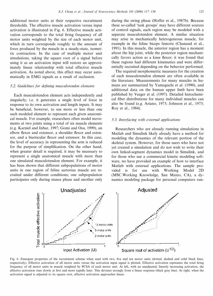
additional motor units at their respective recruitmentthresholds. The effective muscle activation versus inputactivation is illustrated in Fig. 6. Effective muscle acti-vation corresponds to the total firing frequency of allmotor units weighted by the size of each motor unit,which in turn corresponds roughly to the amount offorce produced by the muscle in a steady-state, isomet-ric contraction. In the case of multiple motor unitsimulations, taking the square root of a signal beforeusing it as an activation input will restore an approxi-mately linear relationship with total effective muscleactivation. As noted above, this effect may occur auto-matically in EMG signals as a result of occlusion.

5.2. Guidelines for defining musculotendon elements

Each musculotendon element acts independently andsingularly; i.e. it generates a single level of force inresponse to its own activation and length inputs. It maybe beneficial, however, to use more or less than onesuch modeled element to represent each given anatomi-cal muscle. For example, researchers often model move-ments at two joints using a total of six muscle elements(e.g. Karniel and Inbar, 1997; Gomi and Osu, 1999), anelbow flexor and extensor, a shoulder flexor and exten-sor, and a biarticular flexor and extensor. In this case,the level of accuracy in representing the arm is reducedfor the purpose of simplification. On the other hand,when greater detail is required, it may be necessary torepresent a single anatomical muscle with more thanone simulated musculotendon element. For example, ithas been shown that different subpopulations of motorunits in one region of feline sartorius muscle are re-cruited under different conditions; one subpopulationparticipates only during stance phase and another only

during the swing phase (Hoffer et al., 1987b). Becausethese so-called ‘task groups’ may have different sourcesof control signals, each region may be modeled with aseparate musculotendon element. A similar situationmay arise in mechanically heterogeneous muscle, forexample in the feline biceps femoris (Chanaud et al.,1991). In this muscle, the anterior region has a momentabout the hip joint, while the posterior region mechani-cally favors action as a knee flexor; it was found thatthese regions had different kinematics and were differ-entially recruited depending on the behavior performed.

The required morphometric measures for the creationof each musculotendon element are often available inthe literature. Measurements for many muscles in hu-mans are summarized by Yamaguchi et al. (1990), andadditional data on the human upper limb have beenpublished by Veeger et al. (1997). Detailed histochemi-cal fiber distributions for many individual muscles canalso be found (e.g. Ariano, 1973; Johnson et al., 1973;Roy et al., 1984).

5.3. Interfacing with external applications

Researchers who are already running simulations inMatlab and Simulink likely already have a method formodeling the dynamics of the relevant portion of theskeletal system. However, for those users who have notyet created a simulation and do not wish to write theirown linked-segment dynamics model in Simulink, andfor those who use a commercial kinetic modeling soft-ware, we have provided an example of how to interfaceMatlab with external applications. The sample pro-vided is for use with Working Model 2D(MSC.Working Knowledge, San Mateo, CA), a dy-namics modeling package for personal computers run-

Fig. 6. Emergent properties of the recruitment scheme when used with two, five and ten motor units (dotted, dashed and solid black lines,respectively). Effective activation of all motor units versus the activation input signal is plotted. Effective activation represents the total firingfrequency of all motor units in muscle weighted by PCSA of each motor unit. At left, with an unadjusted, linearly increasing activation, theeffective activation rises slowly at first and more rapidly later. This deviates strongly from a linear response (thick gray line). At right, when theactivation signal is adjusted to its square root, effective activation approaches linear.

E.J. Cheng et al. / Journal of Neuroscience Methods 101 (2000) 117–130126

Fig. 7. (A) ‘Screen shot’ of Working Model 2D running the included sample Dynamics System. Five musculotendon actuators are depicted; twoare attached to the simplified joint model, while the remaining three are not in use. Also displayed are various meters displaying information onactuator lengths and the force that each actuator element exerts. (B) Schematic representation of the structure of the interface between the VirtualMuscle elements (at top) and any external dynamics modeling package (at bottom). The SimDDE function acts as the interface between the twopackages.

6. Discussion

Virtual Muscle should integrate well with existingsimulations designed in Matlab or Simulink, especiallyif the simulations have been designed hierarchically,with separate elements to represent muscle properties.In this case, it may be as simple as replacing an existingrepresentation of musculotendons with Simulink blocksgenerated by Virtual Muscle. On the other hand, simu-lations that lack explicit, independent muscle elementswill not benefit from the Virtual Muscle package aseasily. These simulations are often driven by optimiza-tion criteria relating to net joint torque or stiffnessvalues or cost functions but do not specify explicitly theconstituent muscles. In these cases, models would haveto be significantly redesigned to use realistic musculo-tendon elements. Software and documentation areavailable free via the Internet at http://ami.usc.edu/mddf/virtualmuscle.

Before we created this system to allow the rapidmodification of muscle properties in Matlab and Sim-ulink, we had implemented a similar muscle model inWorking Model 2D alone to examine the implications

ning under Microsoft Windows (Fig. 7). Our inter-ap-plication link utilizes DDE, an interface supported bymany Windows-based applications.

The sample provided uses a wrapper function thatruns in Matlab called SimDDE, which functions to passdata from five Virtual Muscle musculotendon elementsin Simulink to Working Model 2D, and vice-versa (Fig.7). The SimDDE function is called once per simulationtime-step by Working Model 2D, which in turn simu-lates activation (specified in Simulink) and lengthchanges (passed from Working Model 2D) in the Vir-tual Muscle blocks, and returns the forces produced byeach musculotendon element. The SimDDE applicationis fully functional, and any user who wishes to use upto five musculotendon elements can immediately startusing the Virtual Muscle package without further pro-gramming. The muscle database associated with theSimDDE model can be assigned the appropriate musclemorphometry, and the actuator elements within Work-ing Model 2D can be dragged onto the desired skeletalsegments. The simulation is then ready to run fromwithin Working Model 2D.

E.J. Cheng et al. / Journal of Neuroscience Methods 101 (2000) 117–130 127

of realistic muscle properties for motor control (Loeb etal., 1999). Because Working Model 2D is essentially asegment dynamics package, entering the manymathematical equations for each muscle waslabor-intensive, and modifications had to be mademanually for each individual muscle. Modeling multiplemotor units with type-specific properties andindependent frequency modulation was impractical.Since then, we have used the Virtual Muscle packagedescribed here to create and examine a biomechanicalmodel of the arm entirely in Matlab and Simulink,using eight anatomically accurate muscles (Cheng andLoeb, in preparation).

Interfacing with an external dynamics applicationsuch as Working Model 2D obviates the need to codeexplicitly a model of segment dynamics. It isunavoidable, however, that running these twoapplications at the same time is less computationallyefficient than having the muscle and segment dynamicsmodel running in a single package. Thus, users wishingto begin using a motor control simulation need todecide on a balance between performance andsimplicity. Similarly, decisions need to be made whencreating the musculotendon elements as to the level ofcomplexity desired. Each additional motor unitsimulated will increase the computational timerequired, and users need to trade-off speed versusaccuracy. Future directions include adapting portionsof each Virtual Muscle block to run as compiledMatlab code to decrease computational time. While thiswould improve efficiency, it would be at the expense ofcross-platform compatibility.

Acknowledgements

This work was supported by the Medical ResearchCouncil of Canada. We thank Jiping He and StephenScott for assistance in the initial implementation of theequations in Simulink.

Appendix A. Refining the original fiber type model

Our previous work in the two feline muscles soleusand caudofemoralis revealed that the passive forcelength relationship (FPE1) did not scale with L0 betweenmuscle specimens, motivating us to publish severalexamples of parameters for different specimens (Brownet al., 1996b, 1999). Separate work on these and otherhindlimb muscles of the cat revealed that FPE1 scalesmore appropriately with the maximal anatomical lengthof a muscle, Lmax (Brown et al., 1996a). We therefore,combined passive force length data from a total of 61feline hindlimb muscles to determine a single best-fitrelationship based upon data that was normalized to

Lmax (data not reproduced here; soleus data from Scottet al., 1996, semitendinous, sartorius, tenuissimus, bi-ceps femoris anterior and caudofemoralis data fromBrown et al., 1996a, additional caudofemoralis datafrom Brown et al., 1999). Because of the steep slope ofthis relationship and the variability in the x-direction,curve-fitting was accomplished in two steps. First, alldata were shifted in the x-direction (i.e. length) so thatthey aligned at 0.5 F0. The constants responsible for thecurvature (c1 and k1; see Table 1) were then fit to thisshifted data using the standard Levenberg–Marquardtalgorithm. Using these values of c1 and k1, the functionwas then fit to the original non-shifted data to estimatethe best-fit value for Lr1, minimizing error in the x-di-rection (i.e. length). We have also added a small viscos-ity for stability purposes during simulation.

FPE1(L)=c1k1 ln!

exp�(L/Lmax−Lr1)

k1

n+1

"+hV (1)

Equation adapted from Brown et al. (1999). L andLmax must be in the same units (usually L0). Forceoutput is in units of F0.

We have also re-fit our fast-twitch FV relationship.The original data from caudofemoralis (Fig. 6 in Brownet al., 1999) was limited to slow to moderate speeds.Because our curve fitting was not constrained by arealistic Vmax, the curve extrapolated to a Vmax of only7.4 L0/s. Spector et al. (1980) measured Vmax values forfeline soleus and medial gastrocnemius of 4.8 and 12.8L0/s, respectively. We therefore, re-fit our feline caud-ofemoralis FV parameters but with Vmax fixed at 14L0/s (14 L0/s was chosen because caudofemoralis is100% fast-twitch and thus is likely a little faster thanmedial gastrocnemius). This change had a negligibleeffect on the model’s force estimation when comparedwith the original curve derived from the available datafor slow to moderate speeds, but it now extrapolates toa more plausible estimate for fast-twitch Vmax. The newparameters for human muscle are listed in Table 1. (Tocalculate the new feline FV fast-twitch parameters, sim-ply scale the two parameters Vmax and bV by theequivalent change in V0.5 — or let Virtual Muscle do itautomatically).

Appendix B. Estimation of muscle model parameters forhuman skeletal muscle fiber types

Because of the difficulty in performing experimentson human muscles, we have chosen to extrapolate adetailed model of force production in feline muscledescribed previously (Brown and Loeb, 2000; Brown etal., 1999) in order to create a similar model for humanskeletal muscle. The extrapolated parameters for hu-man skeletal muscle fiber types are listed along with theassociated equations in Table 1. We extrapolated the

E.J. Cheng et al. / Journal of Neuroscience Methods 101 (2000) 117–130128

model to human fiber types using the tools described inthis paper, namely by changing optimal sarcomerelength (which scales FL and FPE2), V0.5 (which scalesFV) and f0.5 (which scales feff, which controls rise andfall times). This appendix describes how we estimatedthese values for human fiber types. Although ‘sag’ isnot evident in some human fiber types, (thenar units,Thomas et al., 1991; toe extensor units, Macefield et al.,1996) it is clearly evident in others (triceps surae; vanZandwijk et al., 1998) so we have included it untilfurther evidence can clarify this issue. The limited datafor ‘yielding’ suggest that it, too, is present in at leastsome human muscles (erector spinae, Sutarno andMcGill, 1995).

Optimal sarcomere lengths for various species havebeen published previously by Herzog et al. (1992). Weused their measured values of 2.4 and 2.7 mm for catand human, respectively, to scale the active and passiveforce–length properties.

Estimates of V0.5 and f0.5 were more difficult toobtain. Previous work has shown that Vmax is approxi-mately proportional to contraction time for fiber typesfrom a wide range of species (Close, 1972). Other workhas shown that contraction time is proportional to f0.5.(Kernell et al., 1983; Botterman et al., 1986). Togetherthese imply that V0.5 may be proportional to f0.5 acrossspecies. In Fig. 8 we plot V0.5 versus f0.5 for two felinemuscles composed exclusively of fast-twitch and slow-twitch muscle (upon which the our feline muscle modelwas based), one rat muscle of mostly slow-twitch fibertype composition and two human muscles of mixedfiber type composition (see legend for details). Giventhe similarity in ratios between the various musclesacross fiber types and across species, we have assumedthat for normal muscles the f0.5/V0.5 ratio is constant ata value of 12(pulses/L0).

Based upon this notion of a constant ratio, we needonly acquire f0.5 or V0.5 to define the properties of a‘typical’ fiber type. Single unit data for human musclesare currently extremely sparse and thus unlikely torepresent quantitatively the populations as a whole.Therefore, we have used whole-muscle values alongwith fiber type estimations from Johnson et al. (1973)to estimate different fiber type speeds as a first approx-imation. For adductor pollicus (�80% type I), f0.5 is�14–18 pps (Bigland and Lippold, 1954; Cooper etal., 1988; Rutherford and Jones, 1988). For the quadri-ceps (�45% type I) f0.5 is 16–18 pps (Edwards et al.,1977 — note; original data were collected at a kneeangle of 90°, which is approximately 1.1 L0 (Marshall etal., 1990); therefore, we shifted the reported force–fre-quency relationship assuming the same length depen-dence as feline muscles (Brown et al., 1999)). For firstdorsal interosseus (�55% type I) f0.5 is 12–18 pps,averaged from Milner-Brown et al. (1973b), Rutherfordand Jones (1988). For the triceps surae (�60% type I)f0.5 is �10–12 pps (van Zandwijk et al., 1998). Basedupon these limited data, we tentatively suggest threefiber types, a ‘super’ slow-twitch with f0.5 of �6 pps, a‘typical’ slow-twitch with f0.5 of �12 pps, and a fast-twitch with f0.5 of 20 pps (see Fig. 3B). V0.5 wasestimated at 1/12th those values as described above. Weassume that only the triceps surae muscles contain the‘super slow’ fiber type (analogous to feline soleus) andthat the other muscles described here contain the ‘typi-cal’ slow fiber type. When better data become available,we should be able to improve upon these crudeestimates.

Fig. 8. Frequency–velocity relationship. Relative measures of thefrequency ( f0.5) and velocity (V0.5) are plotted against each other forfive muscles, two each from cat and human and one from rat. ( f0.5 isdefined as the stimulus frequency necessary to produce 0.5 F0 at 1.0L0 during isometric conditions, while V0.5 is the shortening velocitynecessary to produced 0.5 F0 at 1.0 L0 during maximal (tetanicstimulation). The two feline muscles are the exclusively fast-twitchcaudofemoralis (CF) and the exclusively slow-twitch soleus (SOL).The rat muscle is the mostly show SOL. The two human muscles areof mixed composition; first dorsal interossus (FDI) and the quadri-ceps (quads). The data were garnered from the following studies;feline CF V0.5 and f0.5 from Brown et al. (1999); feline SOL V0.5 fromBrown et al. (1996a,b) and f0.5 from Rack and Westbury (1969) asdescribed in Brown et al. (1999); rat SOL V0.5 from Ranatunga (1984)and f0.5 from Binder-Macleod and Barrish (1992) — note, originaldata were collected at the optimal twitch length which is approxi-mately 1.1 L0 (Roszek et al., 1994; Brown and Loeb, 1998) and so weshifted the reported force–frequency relationship assuming the samelength dependence as for feline SOL (Brown et al., 1999); humanquads V0.5 from Marshall et al. (1990) converted from cm to L0 usingan L0 estimate of 9 cm from Scott et al. (1993) and f0.5 from Edwardset al. (1977) — note, original data collected at a knee angle of 90,which is approximately 1.1 L0 based on data from Marshall et al.(1990), therefore, we shifted the reported force-frequency relationshipas per rat SOL above; human FDI V0.5 from Cook and McDonagh(1996) and f0.5 averaged from Milner-Brown et al. (1973a,b), Ruther-ford and Jones (1988).

E.J. Cheng et al. / Journal of Neuroscience Methods 101 (2000) 117–130 129

References

Ariano MA, Armstrong RB, Edgerton VR. Hindlimb muscle fiberpopulations of five mammals. J Histochem Cytochem1973;21:51–5.

Asatryan DG, Feldman AG. Functional tuning of the nervous sys-tem with control of movement or maintenance of a steady pos-ture. I. Mechanographic analysis of the work of the joint orexecution of a postural task. Biofizika 1965;10:837–46.

Balnave CD, Allen DG. The effect of muscle length on intracellularcalcium and force in single fibers from mouse skeletal muscle. JPhysiol 1996;492:705–13.

Bigland B, Lippold OCJ. Motor unit activity in the voluntary con-traction of human muscle. J Physiol 1954;125:322–35.

Binder-Macleod SA, Barrish WJ. Force response of rat soleus mus-cle to variable-frequency train stimulation. J Neurophysiol1992;68:1068–78.

Botterman BR, Iwamoto GA, Gonyea WJ. Gradation of isometrictension by different activation rates in motor units of cat flexorcarpi radialis muscle. J Neurophysiol 1986;56:494–506.

Brown IE. Measured and modeled properties of mammalian skeletalmuscle. Ph.D. thesis, Queen’s University, 1998.

Brown IE, Loeb GE. Post-activation potentiation — a clue forsimplifying models of muscle dynamics. Am Zool 1998;38:743–54.

Brown IE, Loeb GE. Measured and modeled properties of mam-malian skeletal muscle: IV. Dynamics of activation and deactiva-tion, J Muscle Res Cell Motil 2000;21:33–47.

Brown IE, Liinamaa TL, Loeb GE. Relationships between range ofmotion, L0 and passive force in five strap-like muscles of thefeline hindlimb. J Morphol 1996a;230:69–77.

Brown IE, Scott SH, Loeb GE. Mechanics of feline soleus: II.Design and validation of a mathematical model. J Muscle ResCell Motil 1996b;17:219–32.

Brown IE, Satoda T, Richmond FJR, Loeb GE. Feline caudofer-moralis muscle. Muscle fiber properties, architecture, and motorinnervation. Exp Brain Res 1998;121:76–91.

Brown IE, Cheng EJ, Loeb GE. Measured and modeled propertiesof mammalian skeletal muscle: II. The effects of stimulus fre-quency on force–length and force–velocity relationships. J Mus-cle Res Cell Motil 1999;20:627–43.

Chanaud CM, Pratt CA, Loeb GE. Functionally complex musclesof the cat hindlimb. V. The roles of histochemical fiber-typeregionalization and mechanical heterogeneity in differential mus-cle activation. Exp Brain Res 1991;85:300–13.

Close R. Dynamic properties of mammalian skeletal muscle. PhysiolRev 1972:52:129–79.

Cook CS, McDonagh MJ. Force responses to constant-velocityshortening of electrically stimulated human muscle–tendon com-plex. J Appl Physiol 1996;81:384–92.

Cooper RG, Edwards RHT, Gibson H, Stokes MJ. Human musclefatigue: frequency dependence of excitation and force generation.J Physiol 1988;397:585–99.

De Luca CJ, Foley PJ, Erim Z. Motor unit control properties inconstant-force isometric contractions. J Neurophysiol1996;76:1503–16.

Durfee WK, Palmer KI. Estimation of force–activation, force–length, and force–velocity properties in isolated, electricallystimulated muscle. IEEE Trans Biomed Eng 1994;41:205–16.

Edwards RH, Young A, Hosking GP, Jones DA. Human skeletalmuscle function: description of tests and normal values. Clin SciMol Med 1977;52:283–90.

Georgopoulos AP. On reaching. Annu Rev Neurosci 1986;9:147–70.Gomi H, Osu R. Task-dependent viscoelasticity of human multijoint

arm and its spatial characteristics for interaction with environ-ments. J Neurosci 1999;18:8965–78.

Gonzalez RV, Hutchins EL, Barr RE, Abraham LD. Developmentand evaluation of a musculoskeletal model of the elbow jointcomplex. J Biomech Eng 1997;118:32–40.

Gottlieb GL. On the voluntary movement of compliant (inertial-vis-coelastic) loads by parcellated control mechanisms. J Neurophys-iol 1996;76:3207–29.

Henneman E. Organization of the spinal cord. In: Mountcastle B,editor. Medical Physiology, 12th ed. St. Louis: C.V. Mosby Co.,1968:1717–32.

Herzog W, Kamal S, Clarke HD. Myofilament lengths of cat skele-tal muscle: theoretical considerations and functional implica-tions. J Biomech 1992;25:945–8.

Hoffer JA, Sugano N, Loeb GE, Marks WB, O’Donovan MJ, PrattCA. Cat hindlimb motoneurons during locomotion: II. Normalactivity patterns. J Neurophysiol 1987a;57:530–53.

Hoffer JA, Loeb GE, Sugano N, Marks WB, O’Donovan MJ, PrattCA. Cat hindlimb motoneurons during locomotion. III. Func-tional segregation in sartorius. J Neurophysiol 1987b;57:554–62.

Hogan N. The mechanics of multi-joint posture and movementcontrol. Biol Cybern 1985;52:315–31.

Johnson MA, Polgar J, Weightman D, Appleton D. Data on thedistribution of fibre types in thirty-six human muscles. An au-topsy study. J Neurol Sci 1973;18:111–29.

Karniel A, Inbar GF. A model for learning human reaching move-ments. Biol Cybern 1997;77:173–83.

Kaufman KR, An K-N, Litchy WJ, Chao EYS. Physiological pre-diction for muscle forces I. Application to isokinetic exercise.Neuroscience 1991;40:793–804.

Kernell D, Eerbeek O, Verhey BA. Relation between isometric forceand stimulus rate in cat’s hindlimb motor units of differenttwitch contraction times. Exp Brain Res 1983;50:220–7.

Loeb GE, Brown IE, Cheng EJ. A hierarchical foundation formodels of sensorimotor control. Exp Brain Res 1999;126:1–18.

Lucas SM, Ruff RL, Binder MD. Specific tension measurements insingle soleus and medial gastrocnemius muscle fibers of the cat.Exp Neurol 1987;95:142–54.

Macefield VG, Fuglevand AJ, Bigland-Ritchie B. Contractile prop-erties of single motor units in human toe extensors assessed byintraneural motor axon stimulation. J Neurophysiol1996;75:2509–19.

Marshall RN, Mazur SM, Taylor NA. Three-dimensional surfacesfor human muscle kinetics. Eur J Appl Physiol 1990;61:263–70.

Milner-Brown HS, Stein RB, Yemm R. The orderly recruitment ofhuman motor units during voluntary isometric contractions. JPhysiol 1973a;230:359–70.

Milner-Brown HS, Stein RB, Yemm R. Changes in firing rate ofhuman motor units during linearly changing voluntary contrac-tions. J Physiol 1973b;230:371–90.

Osu R, Gomi H. Multijoint muscle regulation mechanisms examinedby measured human arm stiffness and EMG signals. J Neuro-physiol 1999;81:1458–68.

Otten E. A myocybernetic model of the jaw system of the rat. JNeurosci Methods 1987;21:287–302.

Perry J, Bekey GA. EMG–force relationship in skeletal muscle. CritRev Biomed Eng 1981;12:1–22.

Rack PMH, Westbury DR. The effects of length and stimulus rateon tension in the isometric cat soleus muscle. J Physiol1969;204:443–60.

Ranatunga KW. The force–velocity relation of rat fast- and slow-twitch muscles examined at different temperatures. J Physiol1984;351:517–29.

Roszek B, Baan GC, Huijing PA. Decreasing stimulation frequency-dependent length–force characteristics of rat muscle. J ApplPhysiol 1994;77:2115–24.

E.J. Cheng et al. / Journal of Neuroscience Methods 101 (2000) 117–130130

Roy RR, Bello MA, Powell PL, Simpson DR. Architectural design andfiber-type distribution of the major elbow flexors and extensors ofthe monkey (Cynomolgus). Am J Anat 1984;171:285–93.

Rutherford OM, Jones DA. Contractile properties and fatiguability ofthe human adductor pollicis and first dorsal interosseus: a compari-son of the effects of two chronic stimulation patterns. J Neurol Sci1988;85:319–31.

Scott SH, Loeb GE. Mechanical properties of the aponeurosis andtendon of the cat soleus muscle during whole-muscle isometriccontractions. J Morphol 1995;224:73–86.

Scott SH, Engstrom CM, Loeb GE. Morphometry of human thighmuscles. Determination of fascicle architecture by magnetic reso-nance imaging. J Anat 1993;182:249–57.

Scott SH, Brown IE, Loeb GE. Mechanics of feline soleus: I. Effectof fascicle length and velocity on force output. J Muscle Res CellMotil 1996;17:207–19.

Shue G, Crago PE, Chizeck HJ. Muscle-joint models incorporatingactivation dynamics, moment–angle, and moment–velocity prop-erties. IEEE Trans Biomed Eng 1995;42:212–22.

Soechting JF, Flanders M. Evaluating an integrated musculoskeletalmodel of the human arm. J Biomech Eng 1997;119:93–102.

Spector SA, Gardiner PF, Zernicke RF, Roy RR, Edgerton VR.Muscle architecture and force–velocity characteristics of cat soleusand medial gastrocnemius: implications for motor control. JNeurophysiol 1980;44:951–60.

Sutarno CG, McGill SM. Isovelocity investigation of the lengtheningbehavior of the erector spinae muscles. Eur J Appl Physiol1995;70:146–53.

Thomas CK, Johansson RS, Bigland-Ritchie BR. Attempts to physi-ologically classify human thenar motor units. J Neurophysiol1991;65:1501–8.

Todorov E. Direct cortical control of muscle activation in voluntaryarm movements: a model. Nature Neurosci 2000;3:391–8.

van der Helm FCT. Analysis of the kinematic and dynamic behaviorof the shoulder mechanism. J Biomech 1994;27:527–50.

van Zandwijk JP, Bobbert MF, Harlaar J, Hof AL. From twitch totetanus for human muscle: experimental data and model predictionsfor m-triceps surae. Biol Cybern 1998;79:121–30.

Veeger HEJ, Yu B, An K, Rozendal RH. Parameters for modeling theupper extremity. J Biomech 1997;30:647–52.

Yamaguchi GT, Sawa AGU, Moran DW, Fessler MJ, Winters JM.Appendix: a survey of human musculotendon actuator parameters.In: Winters JM, Woo SL-Y, editors. Multiple Muscle Systems:Biomechanics and Movement Organization. New York: Springer,1990:717–73.

Zajac FE. Muscle and tendon, properties, models, scaling and applica-tion to biomechanics and motor control. Crit Rev Biomed Eng1989;17:359–411.

.