VISCOUS-FLOW CALCULATIONS FOR MODEL AND FULL-SCALE …

VISCOUS-FLOW CALCULATIONS FOR MODEL ANDFULL-SCALE CURRENT LOADS ON TYPICAL OFFSHORE

STRUCTURES

A.H. KOOP∗, C.M. KLAIJ# AND G. VAZ#

∗Corresponding author, email: [email protected]∗#Maritime Research Institute Netherlands (MARIN)

P.O. Box 286700 AA Wageningen, The Netherlands

web page: http://www.marin.nl

Key words: CFD, RANS, Current Loads, Verification, Validation, Scale Effects, LNG Carrier, Semi-Submersible

Abstract. In this paper, CFD calculations for current loads on an LNG carrier and a semi-submersibleare presented, both for model and full-scale situations, for current angles ranging from 180 to 0 degrees.MARIN’s in-house URANS code ReFRESCO is used. Numerical studies are carried out concerning itera-tive convergence and grid refinement. In total, more than 100 calculations have been performed. Detailedverification analysis is carried out using modern techniques, and numerical uncertainties are calculated.Afterwards, quantitative validation for model-scale Reynolds number is done taking into account nu-merical and experimental uncertainties. Scale effects on the current coefficients are investigated, havingin mind the estimated numerical uncertainties, and unsteady effects are briefly studied. Good iterativeconvergence is obtained in most calculations, i.e. a decrease in residuals of more than 5 orders is achieved.The sensitivity to grid resolution has been investigated for both model and full scale using five consecu-tively refined grids and for 3 current headings. The differences in the solution between two consecutiverefinements converge for all cases. The numerical uncertainties are larger for angles with small values ofthe loads. Comparison with experiments shows that ReFRESCO provides good quantitative predictionof the current loads at model scale: for angles with larger forces the CFD results are validated with 15%of uncertainty. To determine scale effects the numerical uncertainties must be considered in order toprevent wrong conclusions drawn on basis of numerical differences rather than on physical differences.For the full-scale results larger numerical uncertainties are found than for model scale and for absolutevalues for scale effects this uncertainty should be improved. For the LNG carrier significant scale effects,i.e. more than 40%, have been obtained for current angles where the friction component is dominant.For these cases the numerical uncertainty is relatively low. For the other current angles differences of8− 30% between model and full scale can be observed, but here larger numerical uncertainties are found.For the semi-submersible the numerical uncertainties for the full-scale results are larger than for the LNGcarrier. For the semi-submersible the pressure component of the force is highly dominant, i.e. larger than90% of the total force. On average the full-scale current coefficients are 20% lower than at model scale,but larger differences for a number of angles can be observed.

1 INTRODUCTION

At present, most of the design of offshore structures is done based on current loads coming fromempirical methods or from model-scale experiments. These are usually conservative and therefore ade-quate in this phase. However, there are some counter arguments to this reasoning: 1) for example, afixed cylinder experiences higher loads at super-critical Reynolds numbers than in the drag-crisis at lowerReynolds numbers. Or, as observed in the Current Affairs JIP [1], full-scale average forces on a schematicsemi-submersible are lower than at model scale, but both frequency and amplitudes of full-scale loads arelarger; 2) if one can improve the accuracy of the loads used in the design phase, the safety margins can

1

International Conference on Computational Methods in Marine EngineeringMARINE 2011

L.Eça, E. Oñate, J. García, T. Kvamsdal and P. Bergan (Eds)

Viscous-Flow Calculations for Model and Full-Scale Current Loads on Typical Offshore Structures

94

VISCOUS-FLOW CALCULATIONS FOR MODEL ANDFULL-SCALE CURRENT LOADS ON TYPICAL OFFSHORE

STRUCTURES

A.H. KOOP∗, C.M. KLAIJ# AND G. VAZ#

∗Corresponding author, email: [email protected]∗#Maritime Research Institute Netherlands (MARIN)

P.O. Box 286700 AA Wageningen, The Netherlands

web page: http://www.marin.nl

Key words: CFD, RANS, Current Loads, Verification, Validation, Scale Effects, LNG Carrier, Semi-Submersible

Abstract. In this paper, CFD calculations for current loads on an LNG carrier and a semi-submersibleare presented, both for model and full-scale situations, for current angles ranging from 180 to 0 degrees.MARIN’s in-house URANS code ReFRESCO is used. Numerical studies are carried out concerning itera-tive convergence and grid refinement. In total, more than 100 calculations have been performed. Detailedverification analysis is carried out using modern techniques, and numerical uncertainties are calculated.Afterwards, quantitative validation for model-scale Reynolds number is done taking into account nu-merical and experimental uncertainties. Scale effects on the current coefficients are investigated, havingin mind the estimated numerical uncertainties, and unsteady effects are briefly studied. Good iterativeconvergence is obtained in most calculations, i.e. a decrease in residuals of more than 5 orders is achieved.The sensitivity to grid resolution has been investigated for both model and full scale using five consecu-tively refined grids and for 3 current headings. The differences in the solution between two consecutiverefinements converge for all cases. The numerical uncertainties are larger for angles with small values ofthe loads. Comparison with experiments shows that ReFRESCO provides good quantitative predictionof the current loads at model scale: for angles with larger forces the CFD results are validated with 15%of uncertainty. To determine scale effects the numerical uncertainties must be considered in order toprevent wrong conclusions drawn on basis of numerical differences rather than on physical differences.For the full-scale results larger numerical uncertainties are found than for model scale and for absolutevalues for scale effects this uncertainty should be improved. For the LNG carrier significant scale effects,i.e. more than 40%, have been obtained for current angles where the friction component is dominant.For these cases the numerical uncertainty is relatively low. For the other current angles differences of8− 30% between model and full scale can be observed, but here larger numerical uncertainties are found.For the semi-submersible the numerical uncertainties for the full-scale results are larger than for the LNGcarrier. For the semi-submersible the pressure component of the force is highly dominant, i.e. larger than90% of the total force. On average the full-scale current coefficients are 20% lower than at model scale,but larger differences for a number of angles can be observed.

1 INTRODUCTION

At present, most of the design of offshore structures is done based on current loads coming fromempirical methods or from model-scale experiments. These are usually conservative and therefore ade-quate in this phase. However, there are some counter arguments to this reasoning: 1) for example, afixed cylinder experiences higher loads at super-critical Reynolds numbers than in the drag-crisis at lowerReynolds numbers. Or, as observed in the Current Affairs JIP [1], full-scale average forces on a schematicsemi-submersible are lower than at model scale, but both frequency and amplitudes of full-scale loads arelarger; 2) if one can improve the accuracy of the loads used in the design phase, the safety margins can

1

International Conference on Computational Methods in Marine EngineeringMARINE 2011

L.Eça, E. Oñate, J. García, T. Kvamsdal and P. Bergan (Eds)A.H. Koop, C.M. Klaij and G. Vaz

be reduced decreasing the manufacturing costs of the structures and improving the dynamic-positioningcapabilities. Therefore, there is a real need for full-scale experiments, full-scale calculations or (general)scaling rules. However, full-scale experiments are scarce, difficult to design and to carry out, and whenperformed kept confidential. General scaling rules such as used for ship resistance are not easily devisedfor these kind of complex flows. Thus, currently one is left to full-scale CFD calculations.

Nowadays, most engineers, including the authors, perform CFD at model scale and in steady modeto calculate current coefficients on offshore constructions. Again, the usual reasoning is that scale effectsare small for this type of structures, that model-scale calculations are necessary for validation anyhow,and that unsteady calculations are not needed and/or too expensive. Moreover, usually there is notime/money to perform thorough numerical sensitivity variations, to achieve sufficient iterative conver-gence, and to perform verification studies.

The major objectives of this paper are then fourfold: 1) perform detailed verification studies for modeland full-scale calculations of current loads, on two typical offshore structures, for several current anglesfrom 180 to 0 degrees; 2) validate the model-scale numerical results with experimental data; 3) study thescale effects on the current loads; 4) perform a preliminary study on possible unsteady effects on modeland full-scale loads.

Modern verification and validation techniques [2] are used in order to quantitatively asses numerical,experimental and validation uncertainties. Without those, the accuracy of the numerical results cannotbe determined and conclusions on scale effects cannot be drawn. However, this requires many calculationsand in total more than 100 calculations have been performed.

An LNG carrier appended with bilge-keels and rudder (streamlined body), and a semi-submersibleconstituted by four rounded-square columns mounted on large block-coefficient ship-shaped pontoons(blunt body) are considered, since they are typical offshore constructions. MARIN’s in-house URANScode ReFRESCO [3] is used. Figure 1 presents the geometries and illustrates the calculated flow fieldfor a specific current angle. Previous work done on these structures [1, 4, 5] is here extended, and thelessons learned from the Current Affairs JIP, see [1, 4], are considered in order to improve the accuracyof the results.

The paper is organized as follows. After this introduction, definitions and details on the structures andmeasurements are presented, followed by the numerical settings used for the calculations. Afterwards,and for both the LNG carrier and semi-submersible, the iterative convergence and numerical uncertaintyis discussed followed by detailed validation, and study of scale effects. Additionally, preliminary studieson unsteady effects are shown for the semi-submersible. Finally, major conclusions and further work arepresented.

2 DEFINITIONS

flow

x

α

y

Figure 2: Reference frame

The reference frame and current coefficients are defined followingthe OCIMF [6] convention, see Figure 2: the x-axis points towardsthe bow, the y-axis points towards portside meaning that 180 degreescorresponds to head-on current, 135 degrees to bow-quartering currentand 90 degrees to beam-on current.

The definitions of the force and moment coefficients are given inTable 1. The Reynolds number and Froude number are:

Re =ρUrefLref

µ, Fr =

Uref√gLref

.

The dimensionless current coefficients are:

CX,Y =FX,Y

12ρU

2refLrefT

, CM =MZ

12ρU

2refL

2refT

.

For the LNG carrier the reference length Lref is chosen equal to Lpp. For confidentiality reasons theforce coefficients for the semi-submersible are scaled by the maximum value found in the wind tunnelexperiments. In Section 6 these scaled values are denoted by C∗

X , C∗Y and C∗

M .

2

95

A.H. Koop, C.M. Klaij and G. Vaz

(a) LNG carrier at 140 degrees current heading.

(b) Semi-submersible at 150 degrees current heading.

Figure 1: Impression of the flow field around the LNG carrier and semi-submersible illustrated by thevorticity distribution around the structures.

Table 1: Nomenclature.

α current angle [deg] F = (FX , FY , FZ) forces [kg ·m · s−2]Lpp length between perpendiculars [m] M = (MX ,MY ,MZ) moments [kg ·m2 · s−2]T draft [m] ρ density [kg ·m−3]WD water depth [m] µ dynamic viscosity [kg ·m−1 · s−1]Uref reference velocity [m · s−1] �ω = �× �u vorticity vector [s−1]Lref reference length [m] ω = |�ω| norm of the vorticity vector [s−1]Tref = Lref/Uref reference time [s]

3

96


(a) LNG carrier at 140 degrees current heading.

(b) Semi-submersible at 150 degrees current heading.

Figure 1: Impression of the flow field around the LNG carrier and semi-submersible illustrated by thevorticity distribution around the structures.

Table 1: Nomenclature.

α current angle [deg] F = (FX , FY , FZ) forces [kg ·m · s−2]Lpp length between perpendiculars [m] M = (MX ,MY ,MZ) moments [kg ·m2 · s−2]T draft [m] ρ density [kg ·m−3]WD water depth [m] µ dynamic viscosity [kg ·m−1 · s−1]Uref reference velocity [m · s−1] �ω = �× �u vorticity vector [s−1]Lref reference length [m] ω = |�ω| norm of the vorticity vector [s−1]Tref = Lref/Uref reference time [s]

3


3 MEASUREMENTS

3.1 LNG Carrier

During the HAWAII JIP, current loads for a 135,000 m3 LNG carrier have been measured in MARIN’sshallow water basin by towing the model through otherwise calm water for flow angles between 0 and180 degrees, see [7]. The model of the LNG carrier included bilge keels, propeller and rudder and thescale was 1:50. Studs were used on the bow and stern to trigger the boundary layer to become turbulent.From a Reynolds sensitivity check it was concluded that for the tested current veloctiy, the Reynoldsdependency at model scale on the measured force coefficients was less than 5%. The ratio of the waterdepth to the draft is WD/T = 4.8, indicating that shallow-water effects might have an influence on thecurrent forces, see also [4]. In order for the free-surface effects to be negligible the Froude number was setsmall to Fr = 0.04. During the experiments no significant waves were observed, see [7]. The model-scaleReynolds number is equal to 1.6 ·106. At full scale the Reynolds number is equal to 5 ·108. The full-scaleparticulars of the LNG carrier are given in Table 2.

Table 2: Main particulars of 135,000 m3 LNG carrier

Description Value

Length between perpendiculars Lpp = 274.0mDraft T = 11.0mBreadth B = 44.2mWater-depth WD = 53.0mCapacity 135,000 m3

Current velocity Uref = 2.06m/s

3.2 Semi-submersible

Wind-tunnel tests at Force Technology [8] have been carried out at scale 1:200. The current loadshave been tested in an airflow corresponding to a vertically uniform current. The forces and momentswere measured for angles in the range 0 to 360 degrees in increments of 10 degrees. The tests havebeen carried out with 8 thrusters placed under the pontoons modeled by a single ring. No roughnesswas applied on the hull. Later in the project the semi-submersible was also tested in MARIN’s OffshoreBasin and the length of the pontoons has been changed between the wind tunnel tests and the basinmeasurements. Therefore, the length of the pontoons for the wind tunnel tests was 4.5% shorter thanused in the Offshore Basin and CFD calculations. The comparison between the basin measurements,wind tunnel and CFD results can be found in [5].

The Froude number based on the column diameter at water surface level is equal to Fr = 0.11. TheReynolds number based on Lpp is equal to 2 · 108 at full scale and equal to 5 · 105 in the wind tunnel andmodel-scale CFD calculations. For confidentiality reasons the main particulars of the semi-submersiblecan not be shared in this paper.

4 COMPUTATIONAL SETUP

4.1 Computational grids

For both geometries five consecutively refined block-structured grids have been constructed using thepackage GridPro [9], see Table 3. At model scale the maximum y+ value is below 1 on all grids and nowall functions are used. However, for the LNG carrier at full scale, having y+ values below 1 requiresextremely thin cells, especially close to the bilge keels, which lead to severe numerical problems. Usingthe same clustering as on model scale, we obtain maximum y+ values below 100 and wall functions areapplied. For the semi-submersible the model-scale grids are adapted by refining the first element in theboundary layer to obtain maximum y+ values below 11 and no wall functions are used.

Wall functions model the viscous sublayer near the wall. The use of wall functions effectively avoidsnumerical issues due to extremely thin cells but also introduces an additional modelling error in thecomputations. The effect of using wall functions is not addressed in this paper, but certainly deservesfurther investigation.

4

97


Figure 3: Computational grid for the LNG carrier and semi-submersible. The black lines denote thegrid on the surface of the carrier and the blue lines denote the grid on the water surface.

Table 3: Information on computational grids for the LNG carrier and semi-submersible.

LNG carrier semi-submersiblemodel scale full scale model scale full scale

# cells max y+ max y+ # cells max y+ # cells max y+

very coarse 0.70M 0.95 99.5 0.9M 1.1 1.2M 12coarse 1.15M 0.77 78.5 1.7M 0.81 2.4M 9.0medium 1.85M 0.74 74.8 3.4M 0.62 4.7M 5.8fine 3.33M 0.59 68.1 7.0M 0.53 9.5M 5.0

very fine 5.72M 0.58 61.5 14.0M 0.36 19.3M 4.2

5

98


Figure 3: Computational grid for the LNG carrier and semi-submersible. The black lines denote thegrid on the surface of the carrier and the blue lines denote the grid on the water surface.

Table 3: Information on computational grids for the LNG carrier and semi-submersible.

LNG carrier semi-submersiblemodel scale full scale model scale full scale

# cells max y+ max y+ # cells max y+ # cells max y+

very coarse 0.70M 0.95 99.5 0.9M 1.1 1.2M 12coarse 1.15M 0.77 78.5 1.7M 0.81 2.4M 9.0medium 1.85M 0.74 74.8 3.4M 0.62 4.7M 5.8fine 3.33M 0.59 68.1 7.0M 0.53 9.5M 5.0

very fine 5.72M 0.58 61.5 14.0M 0.36 19.3M 4.2

5


4.2 Boundary and initial conditions

Since the Froude number is very small, wave generation is neglected and a symmetry boundarycondition is imposed on the water surface. The bottom surface of the domain is positioned at the samedepth as in the measurements. For the LNG carrier the water depth to draft ratio is equal to 4.8. In [4]the effect of the distance of the bottom surface has been investigated and it was concluded that for thisratio the bottom surface should be taken into account. Therefore, a free-slip wall condition is prescribedat the bottom surface. For the semi-submersible the water depth to draft ratio is more than 25, so aconstant-pressure boundary condition is prescribed.

In [4], it was shown that the blockage effect of the basin side walls is negligible for the LNG carrier.Therefore, a cylindrical domain is chosen in order to use the same grid for all current angles. The cylinderis centered at the origin and has radius 3.5Lpp for the LNG carrier and 4Lpp for the semi-submersible. Atthe cylindrical boundary a constant uniform velocity is prescribed corresponding with the current angle,together with the eddy-viscosity to laminar-viscosity ratio and the turbulence intensity. For model scalethe turbulence intensity is chosen equal to 1% and the eddy-viscosity ratio is set to 1.0. For full scalethese values are set to 10% and 100.0, respectively. At the outflow, Neumann boundary conditions areapplied for all variables.

For the coarsest grids the initial conditions for the calculations are defined in each computational cellby setting the velocity equal to the constant uniform velocity of the inflow boundary, the pressure ischosen equal to the reference pressure at the outflow boundary and the turbulence intensity and eddy-viscosity ratio equal to the inflow boundary settings. For the calculations on finer grids the solution oncoarser grids is interpolated to the finer grid to serve as the initial condition. This procedure reducescomputational time compared to calculations started from uniform flow.

4.3 ReFRESCO

The CFD calculations in this paper are carried out using MARIN’s in-house viscous-flow URANS codeReFRESCO [3]. ReFRESCO is targeted and optimized for hydrodynamic applications exclusively, and ithas already been applied to several typical offshore flows. In particular, current, wind and manoeuvringcoefficients of semi-submersibles, submarines and ships have been successfully verified and validated,[1, 4, 5, 10, 11]. For all calculations here presented the following numerical settings have been used: 1)QUICK scheme for convection discretization of the momentum equations; 2) Central scheme for diffusiondiscretization; 3) Upwind scheme for convection discretization of the turbulence equations. The SST k-ωturbulence model [12] is used for all calculations. Parallelization has been employed because of the longcomputational times: some calculations have been carried out using 64 quad-core processors.

4.4 Verification and validation procedures

In any numerical calculation there are intrinsic errors which have to be controlled, and if possiblequantified, e.g. iterative and discretization errors. However, for a complex CFD calculation this can bevery time-consuming. Iterative errors are due to non-linear algorithms and iterative solvers utilized, andin principle should be of the same order as the round-off error. Previous studies with two different CFDcodes, see [2], have shown that the iterative error should be at least two orders of magnitude lower thanthe discretization error, in order not to influence the accuracy of the results.

Several methodologies are available to determine the numerical uncertainty related to the discretizationerror [13, 14]. In this paper we follow the approach as described in [2]. The numerical uncertainty Uφ

for any arbitrary flow quantity φ is determined using Uφ = Fs|ε|, where Fs represents a safety factorand ε denotes an estimate of the discretization error. These are determined by applying a least-squaresfit of a error power law, αhp

i , to the results obtained for grids with different densities or relative stepsize hi. The choice of error estimator and safety factor depends on the apparent convergence condition(monotonic, oscillatory, non-convergent) and apparent order of convergence p (see for further details [2]).

Validation can only be done after verification and it involves numerical, experimental and parameteruncertainties. The aim of validation is to estimate the modelling error of a given mathematical modelin relation to a given set of experimental data. If the validation is successful one cannot say that thecode is validated, only that the model is valid for the problem at hand. A well-documented procedure[14] already applied for other ReFRESCO applications [11, 15, 16] is here employed. It compares the

6

99


validation uncertainty Uval with the validation comparison difference E, which are defined by

Uval =√U2φ + U2

inp + U2exp, E = φi − φexp, (1)

with Uφ the numerical uncertainty, Uinp the parameter uncertainty, i.e. uncertainties in the fluid prop-erties, geometry and boundary conditions, and Uexp the experimental uncertainty. φi and φexp representthe numerical and experimental value, respectively. The outcome of the validation exercise is decidedfrom the comparison of |E| with Uval:

- If |E| > Uval, the comparison difference is probably dominated by the modelling error, whichindicates that the model must be improved;

- If |E| < Uval, the modelling error is within the ”noise level” imposed by the three uncertainties.This can mean two things: if E is considered sufficiently small, the model and its solution arevalidated (with Uval precision) against the given experiment; else the quality of the numericalsolution and/or the experiment should be improved before conclusions can be drawn about theadequacy of the mathematical model.

For a precise validation, the experimental uncertainty Uexp is also needed. This is rarely assessed, andfew experimental data for current loads exists in the open-literature for which uncertainties are presented.In this paper, the experimental uncertainty Uexp is assumed to be equal to 5% for the current loadsobtained in MARIN’s shallow-water basin and 10% for those from the wind tunnel. These values are basedon in-house studies taking into account reproducibility for different test runs, manufacturing tolerancesand uncertainties of the sensors. The experimental uncertainty for the wind-tunnel experimental datais larger due to the measurement procedure: the model is placed on a flat splitter plate to position themodel in an uniform airflow. However, along the splitter plate a boundary layer develops which has aninfluence on the forces on the hull.

5 RESULTS FOR LNG CARRIER

5.1 Iterative convergence

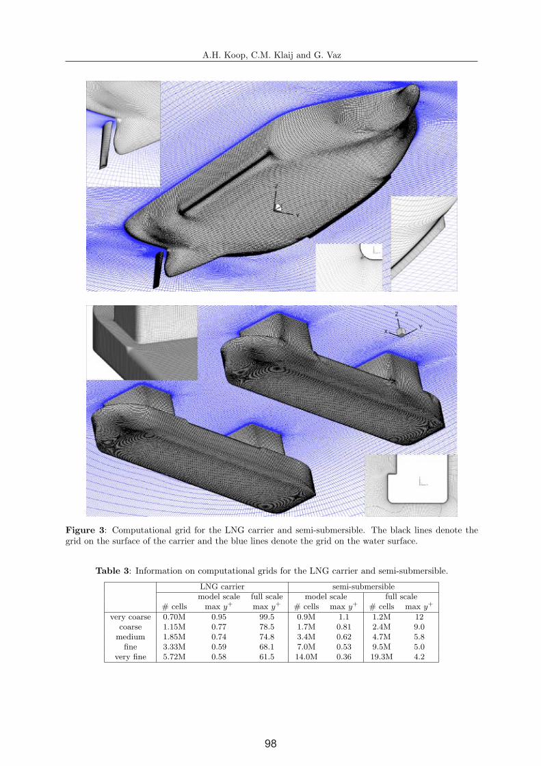
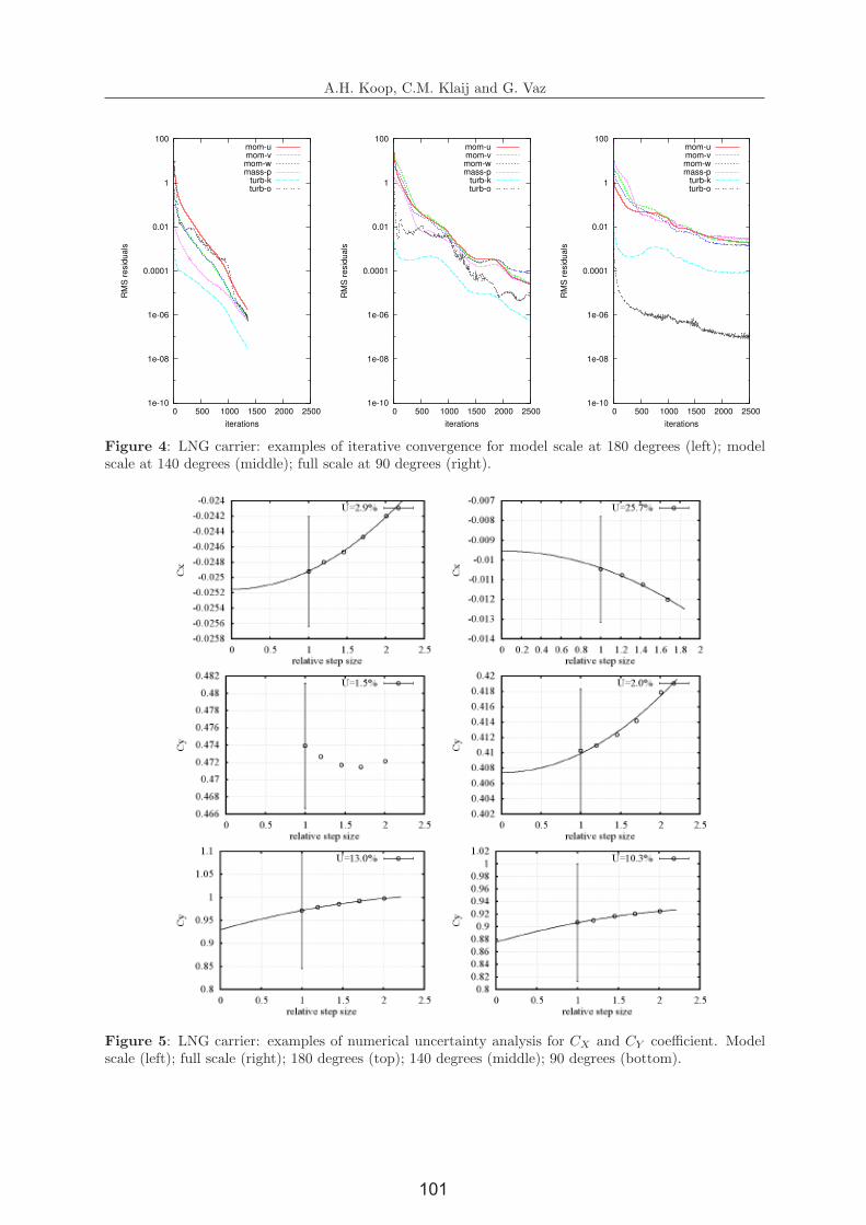
The level and speed of the iterative convergence is dependent on the angle, grid resolution and scaleof the calculation. Figure 4 shows three typical convergence histories: 1) for model scale and 180 degreesthe convergence is fast, and a decrease in residuals more than 6 orders is obtained; 2) for model scale and140 degrees the convergence is slower and the residuals stagnate at 5 orders of decrease; 3) for full scaleat 90 degrees, the convergence history is the worst for all calculations presented in the current paper, andthe residuals stagnate at 3-4 orders. For all cases here presented, the force coefficients become constantafter a few hundred iterations and no oscillations are seen, not even for current angles 140 degrees and90 degrees. In general, full-scale calculations are more difficult to converge than for model scale, and forthe same inflow angle one order less of residuals decrease is obtained.

5.2 Numerical uncertainties

In Table 4 the current loads at model and full scale are presented for three headings using fiveconsecutively refined grids, together with the numerical uncertainties for the finest grid. Figure 5 showsthe results of the uncertainty procedure explained in Section 4.4, for three angles, both for model andfull scale. For the 140 degrees model-scale case the convergence is not monotonic and the uncertaintyprocedure is not able to perform a fit to the error power law. Nevertheless, it is able to estimate anuncertainty value. One can see that the differences in the solution between two consecutive refinementsare getting smaller for all cases, with already relatively small values for the medium grid. However, thishas no relation with the uncertainties calculated, which can still be large.

For model scale the numerical uncertainties are relatively small. In general, the uncertainties arelarger for the coefficients with lower absolute values. At full scale the uncertainties are larger. Also,at full scale, the use of wall-functions adds an additional modeling error which could explain why CX

is more sensitive to grid density than at model scale. The largest sensitivity is found at 140 degreeswhere significant flow separation and recirculation contradict the assumptions underlying wall functions.Notice though, that the uncertainty value of 94.3% for the full-scale CX at 140 degrees, corresponds toa variation of 2× 10−3 in this coefficient, i.e. in absolute magnitude this uncertainty is not relevant.

7

100


validation uncertainty Uval with the validation comparison difference E, which are defined by

Uval =√U2φ + U2

inp + U2exp, E = φi − φexp, (1)

with Uφ the numerical uncertainty, Uinp the parameter uncertainty, i.e. uncertainties in the fluid prop-erties, geometry and boundary conditions, and Uexp the experimental uncertainty. φi and φexp representthe numerical and experimental value, respectively. The outcome of the validation exercise is decidedfrom the comparison of |E| with Uval:

- If |E| > Uval, the comparison difference is probably dominated by the modelling error, whichindicates that the model must be improved;

- If |E| < Uval, the modelling error is within the ”noise level” imposed by the three uncertainties.This can mean two things: if E is considered sufficiently small, the model and its solution arevalidated (with Uval precision) against the given experiment; else the quality of the numericalsolution and/or the experiment should be improved before conclusions can be drawn about theadequacy of the mathematical model.

For a precise validation, the experimental uncertainty Uexp is also needed. This is rarely assessed, andfew experimental data for current loads exists in the open-literature for which uncertainties are presented.In this paper, the experimental uncertainty Uexp is assumed to be equal to 5% for the current loadsobtained in MARIN’s shallow-water basin and 10% for those from the wind tunnel. These values are basedon in-house studies taking into account reproducibility for different test runs, manufacturing tolerancesand uncertainties of the sensors. The experimental uncertainty for the wind-tunnel experimental datais larger due to the measurement procedure: the model is placed on a flat splitter plate to position themodel in an uniform airflow. However, along the splitter plate a boundary layer develops which has aninfluence on the forces on the hull.

5 RESULTS FOR LNG CARRIER


The level and speed of the iterative convergence is dependent on the angle, grid resolution and scaleof the calculation. Figure 4 shows three typical convergence histories: 1) for model scale and 180 degreesthe convergence is fast, and a decrease in residuals more than 6 orders is obtained; 2) for model scale and140 degrees the convergence is slower and the residuals stagnate at 5 orders of decrease; 3) for full scaleat 90 degrees, the convergence history is the worst for all calculations presented in the current paper, andthe residuals stagnate at 3-4 orders. For all cases here presented, the force coefficients become constantafter a few hundred iterations and no oscillations are seen, not even for current angles 140 degrees and90 degrees. In general, full-scale calculations are more difficult to converge than for model scale, and forthe same inflow angle one order less of residuals decrease is obtained.


In Table 4 the current loads at model and full scale are presented for three headings using fiveconsecutively refined grids, together with the numerical uncertainties for the finest grid. Figure 5 showsthe results of the uncertainty procedure explained in Section 4.4, for three angles, both for model andfull scale. For the 140 degrees model-scale case the convergence is not monotonic and the uncertaintyprocedure is not able to perform a fit to the error power law. Nevertheless, it is able to estimate anuncertainty value. One can see that the differences in the solution between two consecutive refinementsare getting smaller for all cases, with already relatively small values for the medium grid. However, thishas no relation with the uncertainties calculated, which can still be large.

For model scale the numerical uncertainties are relatively small. In general, the uncertainties arelarger for the coefficients with lower absolute values. At full scale the uncertainties are larger. Also,at full scale, the use of wall-functions adds an additional modeling error which could explain why CX

is more sensitive to grid density than at model scale. The largest sensitivity is found at 140 degreeswhere significant flow separation and recirculation contradict the assumptions underlying wall functions.Notice though, that the uncertainty value of 94.3% for the full-scale CX at 140 degrees, corresponds toa variation of 2× 10−3 in this coefficient, i.e. in absolute magnitude this uncertainty is not relevant.

7


1e-10

1e-08

1e-06

0.0001

0.01

1

100

0 500 1000 1500 2000 2500

RM

S r

esid

ua

ls

iterations

mom-umom-vmom-wmass-p

turb-kturb-o

1e-10

1e-08

1e-06

0.0001

0.01

1

100

0 500 1000 1500 2000 2500

RM

S r

esid

ua

ls

iterations


turb-kturb-o

1e-10

1e-08

1e-06

0.0001

0.01

1

100

0 500 1000 1500 2000 2500

RM

S r

esid

ua

ls

iterations


turb-kturb-o

Figure 4: LNG carrier: examples of iterative convergence for model scale at 180 degrees (left); modelscale at 140 degrees (middle); full scale at 90 degrees (right).

Figure 5: LNG carrier: examples of numerical uncertainty analysis for CX and CY coefficient. Modelscale (left); full scale (right); 180 degrees (top); 140 degrees (middle); 90 degrees (bottom).

8

101


Table 4: LNG carrier: results for model and full-scale current coefficients at 180, 140 and 90 degreesobtained using grids with different resolution. Between brackets the difference compared to the result onthe finest grid is presented. The numerical uncertainty Uφ for the results of each coefficient for the finestgrid is also presented.

Grid180 degrees 140 degrees 90 degrees

CX CX CY CM CY

Model

scale

very coarse -0.0241 (-3.3%) -0.0137 (-9.0%) 0.4721 (-0.4%) 0.0749 (+4.2%) 0.9978 (+2.7%)coarse -0.0244 (-2.1%) -0.0147 (-13.1%) 0.4714 (-0.6%) 0.0741 (+3.1%) 0.9916 (+2.0%)medium -0.0246 (-1.2%) -0.0156 (-6.0%) 0.4716 (-0.5%) 0.0732 (+1.8%) 0.9855 (+1.4%)fine -0.0248 (-0.4%) -0.0163 (-3.6%) 0.4726 (-0.3%) 0.0719 (0.0%) 0.9781 (+0.6%)

very fine -0.0249 (0.0%) -0.0169 (0.0%) 0.4739 (0.0%) 0.0719 (0.0%) 0.9716 (0.0%)Uφ 2.9% 16.4% 1.5% 3.8% 13.0%

Fullscale

very coarse -0.0120 (-15.4%) 0.00043 (-90%) 0.4178 (+1.8%) 0.0527 (+4.4%) 0.924 (+1.9%)coarse -0.0112 (-7.7%) 0.00200 (-53.4%) 0.4141 (+0.9%) 0.0520 (+3.0%) 0.920 (+1.5%)medium -0.0107 (-2.9%) 0.00312 (-27.3%) 0.4123 (+0.5%) 0.0519 (+2.8%) 0.916 (+1.1%)fine -0.0104 (0.0%) 0.00394 (-8.2%) 0.4109 (+0.1%) 0.0515 (+2.0%) 0.910 (+0.4%)

very fine 0.00429 (0.0%) 0.4102 (0.0%) 0.0505 (0.0%) 0.906 (0.0%)Uφ 25.7% 94.3% 2.0% 12.8% 10.3%

5.3 Validation with model-scale experiments

From the verification exercise presented in Section 5.2 the numerical uncertainty Uφ is known. Havingin the mind the experimental accuracy stated in Section 4.4, the validation procedure can be employed,and the comparison error E and the validation uncertainty Uval can be calculated. Note that, thenumerical uncertainties have been only computed for the angles 180, 140 and 90 degrees. For the sake ofthe validation exercise we consider the maximum value of the uncertainties, for each coefficient, for theremaining angles. This will probably lead to larger validation uncertainties, but also to more validatedresults. For the LNG test-case alone around 40 calculations have been performed in total. In order toobtain Uφ for all angles and both in model and full-scale situations, more than 100 calculations shouldhave been done. Table 5 shows the final results of the validation exercise. Most of the results for CY

are validated within ±15% of uncertainty. It can be observed that for angles where the coefficients havesmall values the CFD results are not validated. The value for CX for 130 degrees shows the use of relativedifferences: the comparison difference E is equal to 165%, which is due to the fact that, coincidentallyfor this angle, the CX coefficient is almost zero.

Table 5: LNG carrier: comparison difference E between model-scale CFD results and experimentalvalues and validation uncertainty Uval. In green the validated results, in red the non-validated results.

CoefficientAngle [deg]

180 170 160 150 140 130 120 110 100 90

ECX -11% -11% -19% -25% +11% +165% +23% +40% +49% -CY - -20% -8% -5% -8% -7% -4% +10% +11% +14%CM - -7% +4% -4% -16% -21% -17% +0.5% +27% -

Uval

CX 15% 15% 13% 12% 18% 43% 20% 23% 25% -CY - 10% 12% 12% 12% 12% 12% 14% 14% 15%CM - 4% 4% 4% 4% 3% 3% 4% 5% -

An extra outcome from the validation procedure is that the graphical comparison between numericaland experimental results can be done using error bars as presented in Figure 6. It can be observed thatthe global trend for the three coefficients is correctly captured by the CFD calculations for the completerange of current angles. Using this graphical presentation of the results, validation is obtained once theuncertainty-bars for both the experiments and numerical results overlap.

9

102


Table 4: LNG carrier: results for model and full-scale current coefficients at 180, 140 and 90 degreesobtained using grids with different resolution. Between brackets the difference compared to the result onthe finest grid is presented. The numerical uncertainty Uφ for the results of each coefficient for the finestgrid is also presented.


CX CX CY CM CY

Model

scale

very coarse -0.0241 (-3.3%) -0.0137 (-9.0%) 0.4721 (-0.4%) 0.0749 (+4.2%) 0.9978 (+2.7%)coarse -0.0244 (-2.1%) -0.0147 (-13.1%) 0.4714 (-0.6%) 0.0741 (+3.1%) 0.9916 (+2.0%)medium -0.0246 (-1.2%) -0.0156 (-6.0%) 0.4716 (-0.5%) 0.0732 (+1.8%) 0.9855 (+1.4%)

fine -0.0248 (-0.4%) -0.0163 (-3.6%) 0.4726 (-0.3%) 0.0719 (0.0%) 0.9781 (+0.6%)very fine -0.0249 (0.0%) -0.0169 (0.0%) 0.4739 (0.0%) 0.0719 (0.0%) 0.9716 (0.0%)

Uφ 2.9% 16.4% 1.5% 3.8% 13.0%

Fullscale

very coarse -0.0120 (-15.4%) 0.00043 (-90%) 0.4178 (+1.8%) 0.0527 (+4.4%) 0.924 (+1.9%)coarse -0.0112 (-7.7%) 0.00200 (-53.4%) 0.4141 (+0.9%) 0.0520 (+3.0%) 0.920 (+1.5%)medium -0.0107 (-2.9%) 0.00312 (-27.3%) 0.4123 (+0.5%) 0.0519 (+2.8%) 0.916 (+1.1%)

fine -0.0104 (0.0%) 0.00394 (-8.2%) 0.4109 (+0.1%) 0.0515 (+2.0%) 0.910 (+0.4%)very fine 0.00429 (0.0%) 0.4102 (0.0%) 0.0505 (0.0%) 0.906 (0.0%)

Uφ 25.7% 94.3% 2.0% 12.8% 10.3%


From the verification exercise presented in Section 5.2 the numerical uncertainty Uφ is known. Havingin the mind the experimental accuracy stated in Section 4.4, the validation procedure can be employed,and the comparison error E and the validation uncertainty Uval can be calculated. Note that, thenumerical uncertainties have been only computed for the angles 180, 140 and 90 degrees. For the sake ofthe validation exercise we consider the maximum value of the uncertainties, for each coefficient, for theremaining angles. This will probably lead to larger validation uncertainties, but also to more validatedresults. For the LNG test-case alone around 40 calculations have been performed in total. In order toobtain Uφ for all angles and both in model and full-scale situations, more than 100 calculations shouldhave been done. Table 5 shows the final results of the validation exercise. Most of the results for CY

are validated within ±15% of uncertainty. It can be observed that for angles where the coefficients havesmall values the CFD results are not validated. The value for CX for 130 degrees shows the use of relativedifferences: the comparison difference E is equal to 165%, which is due to the fact that, coincidentallyfor this angle, the CX coefficient is almost zero.

Table 5: LNG carrier: comparison difference E between model-scale CFD results and experimentalvalues and validation uncertainty Uval. In green the validated results, in red the non-validated results.


180 170 160 150 140 130 120 110 100 90

ECX -11% -11% -19% -25% +11% +165% +23% +40% +49% -CY - -20% -8% -5% -8% -7% -4% +10% +11% +14%CM - -7% +4% -4% -16% -21% -17% +0.5% +27% -

Uval

CX 15% 15% 13% 12% 18% 43% 20% 23% 25% -CY - 10% 12% 12% 12% 12% 12% 14% 14% 15%CM - 4% 4% 4% 4% 3% 3% 4% 5% -

An extra outcome from the validation procedure is that the graphical comparison between numericaland experimental results can be done using error bars as presented in Figure 6. It can be observed thatthe global trend for the three coefficients is correctly captured by the CFD calculations for the completerange of current angles. Using this graphical presentation of the results, validation is obtained once theuncertainty-bars for both the experiments and numerical results overlap.

9


-0.04

-0.02

0

0.02

0.04

0 30 60 90 120 150 180

Cx

Current heading

Experimentmodel-scale CFD

full-scale CFD

0

0.2

0.4

0.6

0.8

1

0 30 60 90 120 150 180

Cy

Current heading


full-scale CFD

-0.1

-0.05

0

0.05

0.1

0.15

0 30 60 90 120 150 180

Cm

Current heading


full-scale CFD

Figure 6: LNG carrier: model and full-scale current coefficients. CFD results versus experimentalresults.

10

103


5.4 Scale effects

The full-scale results show that the force coefficients are typically lower than for model scale asillustrated in Figure 6 and Table 6. This means that the current loads at model scale, either ob-tained using CFD or from experiments, are conservative. In order to distinguish the real physicalscale effects from possible numerical effects, a numerical comparison uncertainty has to be considered

Ucomp =√U2φ,MS + U2

φ,FS . If the difference between model and full-scale results is larger than this

comparison uncertainty then one can say that the scale effect has been captured correctly. If not, noconclusions must be made since the numerical errors taint the real physical effects. As presented in Table6 the comparison uncertainties are too large for CX at 140 degrees and CY at 90 degrees. Nevertheless,we can still, with some carefulness, observe several trends:

• Scale effects are largest when the friction component is dominant. For example, the CX coefficientat 180 degrees is 42%± 26% lower at full scale than at model scale;

• The scale effects for CY are small. For CX the scale effects are larger. For CM it depends on theangle, but they are also clearly visible;

• The scale effect for the friction component is larger than for the pressure component for both CX

and CY . The ratio of the friction component to the pressure component does not remain constantbetween model and full scale;

• Having in mind that the pressure component of the calculated coefficients, except for CX at 180degrees, is larger than the friction component, it is not straightforward to apply the extrapolationtechniques used for ship resistance based on the form-factor hypothesis, see for instance [17].

Table 6: LNG carrier: difference ∆ between model and full-scale values with comparison uncertaintyUcomp. Contribution of pressure (P) and friction (F) to the total force. In green and red the resultswhere Ucomp ≤ ∆ and Ucomp > ∆, respectively.

AngleFS versus MS Model scale Full scale

CX CY CM CX CY CX CY

[deg] ∆ Ucomp ∆ Ucomp ∆ Ucomp P F P F P F P F

180 −42% 26% - - - - 14% 86% - - 14% 86% - -140 −16% 96% −7.8% 2.5% −29% 13% 74% 26% 98% 2% 57% 43% 99% 1%90 - - −3.2% 16% - - - - 99% 1% - - 99% 1%

6 RESULTS FOR SEMI-SUBMERSIBLE


For the semi-submersible the level and speed of the iterative convergence are also dependent on theangle, grid resolution and scale of the calculation. Good convergence is often obtained, i.e. a decreasein residuals of more than 5 orders is achieved as illustrated in Figure 7. However, it also occurs thatthe iterative convergence stagnates at 4 orders. In general, full-scale calculations are more difficult toconverge than for model scale, and for the same inflow angle one order less is obtained. For all cases herepresented, the force coefficients become constant after a few hundred iterations and no oscillations areseen. Compared to the LNG carrier the convergence for the semi-submersible is slower and more difficultto obtain due to the unsteadiness of the flow and complex flow with large separated flow regions.


In Table 7 the results for the semi-submersible without thrusters are presented using subsequentlyrefined grids for model and full scale, all for the angles 180, 150 and 90 degrees. It can be observed thatthe force coefficients converge when using finer grids for all angles both for model and full scale. Also,for all cases the fine grid results are at most 4% different from the results on the very fine grid.

The numerical uncertainties Uφ presented in Table 7 show that for model scale the uncertainties aresmall except for the CX coefficient for 180 degrees and for the CM coefficient for 150 degrees. For 180

11

104


5.4 Scale effects

The full-scale results show that the force coefficients are typically lower than for model scale asillustrated in Figure 6 and Table 6. This means that the current loads at model scale, either ob-tained using CFD or from experiments, are conservative. In order to distinguish the real physicalscale effects from possible numerical effects, a numerical comparison uncertainty has to be considered


φ,FS . If the difference between model and full-scale results is larger than this

comparison uncertainty then one can say that the scale effect has been captured correctly. If not, noconclusions must be made since the numerical errors taint the real physical effects. As presented in Table6 the comparison uncertainties are too large for CX at 140 degrees and CY at 90 degrees. Nevertheless,we can still, with some carefulness, observe several trends:

• Scale effects are largest when the friction component is dominant. For example, the CX coefficientat 180 degrees is 42%± 26% lower at full scale than at model scale;

• The scale effects for CY are small. For CX the scale effects are larger. For CM it depends on theangle, but they are also clearly visible;

• The scale effect for the friction component is larger than for the pressure component for both CX

and CY . The ratio of the friction component to the pressure component does not remain constantbetween model and full scale;

• Having in mind that the pressure component of the calculated coefficients, except for CX at 180degrees, is larger than the friction component, it is not straightforward to apply the extrapolationtechniques used for ship resistance based on the form-factor hypothesis, see for instance [17].

Table 6: LNG carrier: difference ∆ between model and full-scale values with comparison uncertaintyUcomp. Contribution of pressure (P) and friction (F) to the total force. In green and red the resultswhere Ucomp ≤ ∆ and Ucomp > ∆, respectively.


CX CY CM CX CY CX CY


180 −42% 26% - - - - 14% 86% - - 14% 86% - -140 −16% 96% −7.8% 2.5% −29% 13% 74% 26% 98% 2% 57% 43% 99% 1%90 - - −3.2% 16% - - - - 99% 1% - - 99% 1%

6 RESULTS FOR SEMI-SUBMERSIBLE


For the semi-submersible the level and speed of the iterative convergence are also dependent on theangle, grid resolution and scale of the calculation. Good convergence is often obtained, i.e. a decreasein residuals of more than 5 orders is achieved as illustrated in Figure 7. However, it also occurs thatthe iterative convergence stagnates at 4 orders. In general, full-scale calculations are more difficult toconverge than for model scale, and for the same inflow angle one order less is obtained. For all cases herepresented, the force coefficients become constant after a few hundred iterations and no oscillations areseen. Compared to the LNG carrier the convergence for the semi-submersible is slower and more difficultto obtain due to the unsteadiness of the flow and complex flow with large separated flow regions.


In Table 7 the results for the semi-submersible without thrusters are presented using subsequentlyrefined grids for model and full scale, all for the angles 180, 150 and 90 degrees. It can be observed thatthe force coefficients converge when using finer grids for all angles both for model and full scale. Also,for all cases the fine grid results are at most 4% different from the results on the very fine grid.

The numerical uncertainties Uφ presented in Table 7 show that for model scale the uncertainties aresmall except for the CX coefficient for 180 degrees and for the CM coefficient for 150 degrees. For 180

11


1e-08

1e-07

1e-06

1e-05

0.0001

0.001

0.01

0.1

1

10

0 2000 4000 6000 8000 10000

RM

S r

esid

ua

ls

outer iterations


turb-kturb-o

1e-08

1e-07

1e-06

1e-05

0.0001

0.001

0.01

0.1

1

10

0 2000 4000 6000 8000 10000

RM

S r

esid

ua

ls

outer iterations


turb-kturb-o

Figure 7: Semi-submersible: examples of iterative convergence for model scale at 90 degrees (left) andfull scale at 180 degrees (right).

Figure 8: Semi-submersible: examples of numerical uncertainty analysis for CX and CY coefficient.(left) Model scale (right) Full scale.

12

105


degrees the drag force is very small, leading to a higher uncertainty similar to as found for the LNGcarrier. The moment on the semi-submersible is sensitive to the precise location of the flow separation.When refining the grid this location changes slightly leading to a change in the moment. The numericaluncertainties for the full-scale calculations are higher than for model scale.

Table 7: Semi-submersible without thrusters: results for model and full-scale current at 180, 150 and 90degrees obtained using grids with different resolution. Between brackets the difference compared to theresult on the finest grid is presented. The numerical uncertainty Uφ for the results of each coefficient forthe finest grid is also presented.


C∗X C∗

X C∗Y C∗

M C∗Y

Model

scale

very coarse 0.651 (+14.8%) 0.810 (+3.1%) 0.439 (-5.8%) 0.725 (+28.9%) 0.677 (+0.9%)coarse 0.642 (+13.2%) 0.799 (+1.7%) 0.444 (-4.7%) 0.693 (+23.1% 0.670 (-0.1%)medium 0.612 (+7.9%) 0.787 (+0.1%) 0.459 (-1.5%) 0.614 (+9.1%) 0.664 (-1.0%)fine 0.590 (+4.1%) 0.786 (0.0%) 0.467 (+0.2%) 0.565 (+0.4%) 0.672 (+0.1%)

very fine 0.566 (0.0%) 0.786 (0.0%) 0.466 (0.0%) 0.563 (0.0%) 0.671 (0.0%)Uφ 29.5% 2.2% 5.5% 31.6% 3.7%

Fullscale

very coarse 0.484 (+5.0%) 0.782 (+8.0%) 0.390 (+16.8%) 0.946 (+35.4%) 0.623 (+11.8%)coarse 0.490 (+6.3%) 0.771 (+6.6%) 0.385 (+15.3%) 0.890 (+27.3%) 0.598 (+7.5%)medium 0.476 (+3.3%) 0.748 (+3.3%) 0.373 (+12.0%) 0.735 (+5.1%) 0.580 (+4.1%)fine 0.471 (+2.2%) 0.732 (+1.1%) 0.348 (+4.2%) 0.712 (+1.9%) 0.567 (+1.8%)

very fine 0.461 (0.0%) 0.724 (0.0%) 0.334 (0.0%) 0.699 (0.0%) 0.557 (0.0%)Uφ 12.4% 21.8% 33.1% 19.7% 6.2%


In the wind-tunnel experiments eight thrusters were modelled under the hull of the semi-submersible.For validation purposes it would have been better to test and calculate the bare hull of the semi-submersible. In [5] the effect of modeling the thrusters has been investigated and it was concludedthat for certain current headings the thrusters have a significant effect on the calculated results. There-fore, for the comparison between the CFD and wind tunnel results, following [5], the thrusters have beentaken into account in the CFD calculations presented in Figure 9 and Table 8. However, in the wind tun-nel simple rings were used for the thrusters. In the CFD calculations the exact geometry of the thrustershas been taken into account but the thrusters have been closed. This leads to an additional uncertaintywhen comparing the results between wind tunnel and CFD, which can be taken into account throughthe parameter uncertainty Uinp in Equation 1. We assume that this uncertainty due to the thrusters is4%. Furthermore, as explained in Section 3.2, the pontoons in the wind tunnel were 4.5% shorter thanin the CFD calculations. This leads to approximately 1% larger drag forces and 3% larger side forces inthe CFD calculations. Therefore, we assume that the total value for the parameter uncertainty Uinp isequal to 8%.

From Figure 9 it appears that good agreement between the wind tunnel and CFD is obtained. Forthe angles with larger forces, i.e. the range 180 to 130 degrees for C∗

X and the range 140 to 90 degrees forC∗

Y , the CFD results are validated and within 12% or lower from the wind tunnel results. However, forC∗

X the validation uncertainty Uval is large and both the numerical and experimental uncertainty shouldbe decreased.

Table 8: Semi-submersible with thrusters: comparison difference E between model-scale CFD resultsand experimental values and validation uncertainty Uval. In green the validated results and in red thenon-validated results.


180 170 160 150 140 130 120 110 100 90

EC∗

X +9% +16% +4% -2% -12% -9% -35% -46% -73% -C∗

Y - -27% -27% -15% -8% -12% -10% -11% -11% -11%

UvalC∗

X 35% 37% 33% 13% 29% 30% 22% 19% 13% 10%C∗

Y 10% 12% 12% 13% 13% 13% 13% 13% 13% 13%

13

106


degrees the drag force is very small, leading to a higher uncertainty similar to as found for the LNGcarrier. The moment on the semi-submersible is sensitive to the precise location of the flow separation.When refining the grid this location changes slightly leading to a change in the moment. The numericaluncertainties for the full-scale calculations are higher than for model scale.

Table 7: Semi-submersible without thrusters: results for model and full-scale current at 180, 150 and 90degrees obtained using grids with different resolution. Between brackets the difference compared to theresult on the finest grid is presented. The numerical uncertainty Uφ for the results of each coefficient forthe finest grid is also presented.


C∗X C∗

X C∗Y C∗

M C∗Y

Model

scale

very coarse 0.651 (+14.8%) 0.810 (+3.1%) 0.439 (-5.8%) 0.725 (+28.9%) 0.677 (+0.9%)coarse 0.642 (+13.2%) 0.799 (+1.7%) 0.444 (-4.7%) 0.693 (+23.1% 0.670 (-0.1%)medium 0.612 (+7.9%) 0.787 (+0.1%) 0.459 (-1.5%) 0.614 (+9.1%) 0.664 (-1.0%)fine 0.590 (+4.1%) 0.786 (0.0%) 0.467 (+0.2%) 0.565 (+0.4%) 0.672 (+0.1%)

very fine 0.566 (0.0%) 0.786 (0.0%) 0.466 (0.0%) 0.563 (0.0%) 0.671 (0.0%)Uφ 29.5% 2.2% 5.5% 31.6% 3.7%

Fullscale

very coarse 0.484 (+5.0%) 0.782 (+8.0%) 0.390 (+16.8%) 0.946 (+35.4%) 0.623 (+11.8%)coarse 0.490 (+6.3%) 0.771 (+6.6%) 0.385 (+15.3%) 0.890 (+27.3%) 0.598 (+7.5%)medium 0.476 (+3.3%) 0.748 (+3.3%) 0.373 (+12.0%) 0.735 (+5.1%) 0.580 (+4.1%)fine 0.471 (+2.2%) 0.732 (+1.1%) 0.348 (+4.2%) 0.712 (+1.9%) 0.567 (+1.8%)

very fine 0.461 (0.0%) 0.724 (0.0%) 0.334 (0.0%) 0.699 (0.0%) 0.557 (0.0%)Uφ 12.4% 21.8% 33.1% 19.7% 6.2%


In the wind-tunnel experiments eight thrusters were modelled under the hull of the semi-submersible.For validation purposes it would have been better to test and calculate the bare hull of the semi-submersible. In [5] the effect of modeling the thrusters has been investigated and it was concludedthat for certain current headings the thrusters have a significant effect on the calculated results. There-fore, for the comparison between the CFD and wind tunnel results, following [5], the thrusters have beentaken into account in the CFD calculations presented in Figure 9 and Table 8. However, in the wind tun-nel simple rings were used for the thrusters. In the CFD calculations the exact geometry of the thrustershas been taken into account but the thrusters have been closed. This leads to an additional uncertaintywhen comparing the results between wind tunnel and CFD, which can be taken into account throughthe parameter uncertainty Uinp in Equation 1. We assume that this uncertainty due to the thrusters is4%. Furthermore, as explained in Section 3.2, the pontoons in the wind tunnel were 4.5% shorter thanin the CFD calculations. This leads to approximately 1% larger drag forces and 3% larger side forces inthe CFD calculations. Therefore, we assume that the total value for the parameter uncertainty Uinp isequal to 8%.

From Figure 9 it appears that good agreement between the wind tunnel and CFD is obtained. Forthe angles with larger forces, i.e. the range 180 to 130 degrees for C∗

X and the range 140 to 90 degrees forC∗

Y , the CFD results are validated and within 12% or lower from the wind tunnel results. However, forC∗

X the validation uncertainty Uval is large and both the numerical and experimental uncertainty shouldbe decreased.

Table 8: Semi-submersible with thrusters: comparison difference E between model-scale CFD resultsand experimental values and validation uncertainty Uval. In green the validated results and in red thenon-validated results.


180 170 160 150 140 130 120 110 100 90

EC∗

X +9% +16% +4% -2% -12% -9% -35% -46% -73% -C∗

Y - -27% -27% -15% -8% -12% -10% -11% -11% -11%

UvalC∗

X 35% 37% 33% 13% 29% 30% 22% 19% 13% 10%C∗

Y 10% 12% 12% 13% 13% 13% 13% 13% 13% 13%

13


-0.4

-0.2

0

0.2

0.4

0.6

0.8

1

90 120 150 180

Cx*

Current heading

Wind tunnelModel-scale CFD -0.2

0

0.2

0.4

0.6

0.8

1

1.2

90 120 150 180

Cy*

Current heading

Wind tunnelModel-scale CFD

Figure 9: Semi-submersible with thrusters: comparison of CFD results with experimental results.

6.4 Scale effects

Scale effects are determined for the semi-submersible without thrusters using the fine grid for bothmodel and full scale. It can be observed in Figure 10 and Table 9 that for the angles with larger C∗

X value,i.e. the angles from 180 to 120 degrees, the difference between model scale and full scale is approximately6-30%.

For the angles with larger C∗Y values, i.e. the angles from 160 to 90 degrees, the difference is larger:

6-43%. It should be noted that the pressure component of the force for the semi is highly dominant, i.e.more than 90% of the total force originates from the pressure distribution on the semi, even for the C∗

X

at 180 degrees. This is due to the blunt-body shape of the structure. The ratio between the pressure andfriction component changes slightly from model to full scale.

When considering the difference ∆ between model and full-scale results and the comparison uncertainty


φ,FS , as presented in Table 9, we conclude that the scale effects have been captured

correctly for C∗Y since the difference ∆ is larger than the comparison uncertainty. For C∗

X and C∗M the

numerical uncertainty of the full-scale results are large indicating that one should be careful to drawstrong conclusions based on these full-scale results.

Table 9: Semi-submersible without thrusters: difference between model and full-scale values and con-tribution of pressure (P) and friction (F) to the total force. Results obtained on fine grid. In green andred the results where Ucomp ≤ ∆ and Ucomp > ∆, respectively.


C∗X C∗

Y C∗M C∗

X C∗Y C∗

X C∗Y


180 -20% 32% - - - - 90% 10% - - 95% 5% - -150 -9% 22% -36% 33% +20% 37% 92% 8% 98% 2% 97% 3% 99% 1%90 - - -19% 7% - - - - 98% 2% - - 99% 1%

6.5 Unsteady calculations

To investigate the change in forces due to unsteady effects preliminary unsteady URANS calculationsare carried out. These calculations require large CPU time, and for practical applications they are usuallynot performed. The results here presented are for both model and full scale for current headings 180 and150 degrees. For 180 degrees the flow is very unsteady due to vortices being shed from the first columnswhich interfere with the columns located in the wake. At 150 degrees significant flow separation occurscharacterized by large, steady, coherent vortices along the keel of the semi-submersible resulting in a verysteady flow pattern. Different grid resolution and time step sizes are used: the medium, fine and veryfine grid together with time step sizes equal to Tref/50, Tref/100 and Tref/200 with Tref the reference timehere defined by D/Uref . In the near future the same investigations for heading 90 degrees will be carriedout.

During the unsteady calculations the level of iterative convergence is aimed to be lower than 10−4

as visible in Figure 11(a). The number of iterations per time step have an influence on the level of

14

107


-0.4

-0.2

0

0.2

0.4

0.6

0.8

1

90 120 150 180

Cx*

Current heading

Model-scale CFDFull-scale CFD

-0.2

0

0.2

0.4

0.6

0.8

1

1.2

90 120 150 180

Cy*

Current heading


-0.5

0

0.5

1

1.5

2

2.5

90 120 150 180

Cm

*

Current heading


Figure 10: Semi-submersible without thrusters: model and full-scale current coefficients.

15

108


-0.4

-0.2

0

0.2

0.4

0.6

0.8

1

90 120 150 180

Cx*

Current heading


-0.2

0

0.2

0.4

0.6

0.8

1

1.2

90 120 150 180

Cy*

Current heading


-0.5

0

0.5

1

1.5

2

2.5

90 120 150 180

Cm

*

Current heading


Figure 10: Semi-submersible without thrusters: model and full-scale current coefficients.

15


(a)

(b)

(c)

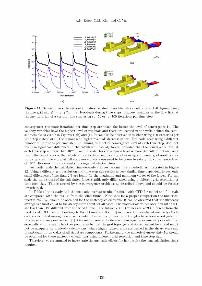
Figure 11: Semi-submersible without thrusters: unsteady model-scale calculations at 180 degrees usingthe fine grid and ∆t = Tref/50 . (a) Residuals during time steps. Highest residuals in the flow field atthe last iteration of a certain time step using (b) 50 or (c) 100 iterations per time step.

convergence: the more iterations per time step are taken the better the level of convergence is. Thevelocity variables have the highest level of residuals and these are located in the wake behind the semi-submersible as visible in Figures 11(b) and (c). It can also be observed that when using 100 iterations pertime step instead of 50, the regions with higher residuals decrease in size. For model scale using a differentnumber of iterations per time step, i.e. aiming at a better convergence level at each time step, does notresult in significant differences in the calculated unsteady forces, provided that the convergence level ateach time step is lower than 10−4. For full scale this convergence level is more difficult to obtain. As aresult the time traces of the calculated forces differ significantly when using a different grid resolution ortime step size. Therefore, at full scale more outer loops need to be taken to satisfy the convergence levelof 10−4. However, this also results in longer calculation times.

For model scale the calculated time-dependent forces become nicely periodic as illustrated in Figure12. Using a different grid resolution and time step size results in very similar time-dependent forces, onlysmall differences of less than 2% are found for the maximum and minimum values of the forces. For fullscale the time traces of the calculated forces significantly differ when using a different grid resolution ortime step size. This is caused by the convergence problems as described above and should be furtherinvestigated.

In Table 10 the steady and the unsteady average results obtained with CFD for model and full scaleare compared with the results from the wind tunnel. Note that for a proper comparison the numericaluncertainty Uphi should be obtained for the unsteady calculations. It can be observed that the unsteadyaverage is almost equal to the steady-state result for all cases. The model-scale values obtained with CFDare less than 11% different from the wind tunnel. The full-scale CFD values are 7-29% different from themodel-scale CFD values. Contrary to the obtained results in [1] we do not find significant unsteady effectson the calculated average force coefficients. However, only two current angles have been investigated inthis paper and only one angle in [1]. One major issue is the iterative convergence for unsteady calculations,especially at full scale. The other point may be that the grid topology and its refinement here used mightnot be adequate for unsteady calculations, where highly refined grids are needed in the shear-layers andin particular in the wakes of all structure components. Furthermore, the numerical uncertainty Uφ shouldbe obtained for these unsteady calculations using different grid resolution and time step size.

Therefore, we recommend to investigate the unsteady effects further despite the long calculation timesrequired.

16

109


(a) C∗X (b) C∗

Y

Figure 12: Semi-submersible without thrusters: unsteady model and full-scale force coefficients at 180degrees.

Table 10: Semi-submersible without thrusters: results for current coefficients at 180 and 150 degrees.The steady results and the unsteady average are compared with the results from the wind tunnel. Thefull-scale values obtained with CFD are compared to the model-scale CFD results.

180 degrees 150 degreesC∗

X C∗X C∗

Y C∗M

Windtunnel - - - -Steady MS +1% -11% -9% +3%

Unsteady MS +4% -11% -9% +6%

Steady FS -20% -7% -26% +29%Unsteady FS -22% -7% -24% +22%

7 CONCLUSIONS AND FUTURE WORK

In this paper, CFD calculations for current loads on an LNG carrier and a semi-submersible arepresented, both for model and full-scale situations, for current angles ranging from 180 to 0 degrees.MARIN’s in-house URANS code ReFRESCO is used. Numerical studies are carried out concerningiterative convergence and grid refinement. In total, more than 100 calculations have been performed.Detailed verification analysis is carried out using modern techniques, and numerical uncertainties arecalculated. Afterwards, quantitative validation for model-scale Reynolds number is done. Scale effectson the current coefficients are investigated, having in mind the estimated numerical uncertainties, andunsteady effects are briefly studied.

Good iterative convergence is obtained in most calculations, i.e. a decrease in residuals of more than 5orders is achieved. The level and speed of the iterative convergence is dependent on the current angle, gridresolution and scale of the calculation. Nicely streamlined flows are easier to solve than flows with largeseparated flow regions. Full-scale calculations are more difficult to converge than for model scale and forthe same flow angle one order less is obtained. For unsteady model-scale calculations a better iterativeconvergence level does not result in significant changes in the calculated unsteady forces, provided thatthe convergence level at each time step is lower than 10−4. For full scale this convergence level is moredifficult to obtain and more iterations per time step should be taken to satisfy this convergence level.However, the authors emphasize that an adequate absolute value for iterative convergence is very muchdependent on the employed linear solvers, residual normalization and numerical tool.

The sensitivity to grid resolution at model and full scale has been investigated for both cases usingfive consecutively refined grids and for 3 current headings. The differences in the solution between twoconsecutive refinements converge for all cases. The fine grid results, i.e. 3 million cells for the LNG carrierand 7 million cells for the semi-submersible, are at most 4% different from the results on the very-finegrid with 6 million cells for the LNG carrier and 20 million cells for the semi-submersible. However, thisdoes not mean that the numerical uncertainties are low. The numerical uncertainties are larger for angles

17

110


(a) C∗X (b) C∗

Y

Figure 12: Semi-submersible without thrusters: unsteady model and full-scale force coefficients at 180degrees.

Table 10: Semi-submersible without thrusters: results for current coefficients at 180 and 150 degrees.The steady results and the unsteady average are compared with the results from the wind tunnel. Thefull-scale values obtained with CFD are compared to the model-scale CFD results.

180 degrees 150 degreesC∗

X C∗X C∗

Y C∗M

Windtunnel - - - -Steady MS +1% -11% -9% +3%

Unsteady MS +4% -11% -9% +6%

Steady FS -20% -7% -26% +29%Unsteady FS -22% -7% -24% +22%

7 CONCLUSIONS AND FUTURE WORK

In this paper, CFD calculations for current loads on an LNG carrier and a semi-submersible arepresented, both for model and full-scale situations, for current angles ranging from 180 to 0 degrees.MARIN’s in-house URANS code ReFRESCO is used. Numerical studies are carried out concerningiterative convergence and grid refinement. In total, more than 100 calculations have been performed.Detailed verification analysis is carried out using modern techniques, and numerical uncertainties arecalculated. Afterwards, quantitative validation for model-scale Reynolds number is done. Scale effectson the current coefficients are investigated, having in mind the estimated numerical uncertainties, andunsteady effects are briefly studied.

Good iterative convergence is obtained in most calculations, i.e. a decrease in residuals of more than 5orders is achieved. The level and speed of the iterative convergence is dependent on the current angle, gridresolution and scale of the calculation. Nicely streamlined flows are easier to solve than flows with largeseparated flow regions. Full-scale calculations are more difficult to converge than for model scale and forthe same flow angle one order less is obtained. For unsteady model-scale calculations a better iterativeconvergence level does not result in significant changes in the calculated unsteady forces, provided thatthe convergence level at each time step is lower than 10−4. For full scale this convergence level is moredifficult to obtain and more iterations per time step should be taken to satisfy this convergence level.However, the authors emphasize that an adequate absolute value for iterative convergence is very muchdependent on the employed linear solvers, residual normalization and numerical tool.

The sensitivity to grid resolution at model and full scale has been investigated for both cases usingfive consecutively refined grids and for 3 current headings. The differences in the solution between twoconsecutive refinements converge for all cases. The fine grid results, i.e. 3 million cells for the LNG carrierand 7 million cells for the semi-submersible, are at most 4% different from the results on the very-finegrid with 6 million cells for the LNG carrier and 20 million cells for the semi-submersible. However, thisdoes not mean that the numerical uncertainties are low. The numerical uncertainties are larger for angles

17


with small values of the loads, which is also expected for the experimental results. In some cases, such asCX for 180 degrees current heading at model-scale, the numerical uncertainty value is too large, 29.5%.In order to further decrease the numerical uncertainties, better iterative convergence should be achievedand even finer grids should be used. In general, for full-scale situations the numerical uncertainties arehigher. Also, for full-scale situations no wall-functions should be used, since this adds an additionalmodelling inaccuracy, and possibility of numerical scattering due to different boundary conditions fordifferent grids.

Comparison with experiments shows that ReFRESCO provides good quantitative prediction of thecurrent loads at model scale. Taking into account the numerical and experimental uncertainties, it is foundthat for angles with larger forces the CFD results are validated with 15% of uncertainty. Nevertheless,for the semi-submersible, for some validated situations, the validation uncertainties are too large due tothe numerical uncertainties, but also due to the large experimental and input-parameters uncertainties.This should be further investigated.

To determine scale effects the numerical uncertainties must be considered in order to prevent wrongconclusions drawn on basis of numerical differences rather than on physical differences. When the dif-ference between model and full-scale results is smaller than the comparison uncertainty these valuesshould be considered with care. For the full-scale results larger numerical uncertainties are found thanfor model scale and for absolute values for scale effects this uncertainty should be improved. For theLNG carrier significant scale effects, i.e. more than 40%, have been obtained for current angles wherethe friction component is dominant. For these cases the numerical uncertainty is relatively low. For theother current angles differences of 8-30% between model and full scale can be observed, but here largeruncertainties are found. For the semi-submersible the numerical uncertainties for the full-scale results arelarger than for the LNG carrier. For the semi-submersible the pressure component of the force is highlydominant, i.e. larger than 90% of the total force. On average the full-scale current coefficients are 20%lower than at model scale, but larger differences for a number of angles can be observed. For both thesemi-submersible and the LNG carrier it is found that the ratio between the pressure contribution andfriction contribution to the force does not remain constant comparing model scale to full scale. For theangles where the pressure component is larger than the friction component, it is not straightforward toapply extrapolation methods as used for ship resistance.

Lastly, a preliminary study into the unsteady effects on the current loads has been carried out. Thesecalculations require much CPU time and are therefore only presented for 180 and 150 degrees currentheading. Contrary to the obtained results from [1] we do not find significant unsteady effects on theaverage of the calculated force coefficients. However, only two current angles have been investigated inthis paper and only one angle in [1]. More calculations for different headings should be carried out beforea valid conclusion on unsteady effects can be drawn. Unsteady problems can be found in many offshoreapplications such as Vortex Induced Motions (VIM), illustrating the importance to accurately calculatethe unsteady flow. Therefore, we recommend to further investigate the unsteady effects despite the longcalculation times required.

18

111


REFERENCES

[1] G. Vaz, O. Waals, F. Fathi, H. Ottens, T. Le Souef, and K. Kwong. Current Affairs - Model Tests,Semi-Empirical Predictions and CFD Computations for Current Coefficients of Semi-Submersibles.In Proceedings of OMAE2009, Honolulu, Hawaii, USA, June 2009.

[2] L. Eca, G. Vaz, and M. Hoekstra. A Verification and Validation Exercise for the Flow Over aBackward Facing Step. In Proceedings of ECCOMAS-CFD2010, Lisbon, Portugal, June 2010.

[3] G. Vaz, F. Jaouen, and M. Hoekstra. Free-Surface Viscous Flow Computations. Validation of URANSCode FreSCo. In Proceedings of OMAE2009, Honolulu, Hawaii, USA, June 2009.

[4] F. Fathi, C.M. Klaij, and A. Koop. Predicting Loads on a LNG Carrier with CFD. In Proceedingsof OMAE2010, Shanghai, China, June 2010.

[5] A. Koop and A. Bereznitski. Model-Scale and Full-Scale CFD Calculations for Current Loads onSemi-Submersible. In Proceedings of OMAE2011, Rotterdam, the Netherlands, June 2011.

[6] Oil Companies International Marine Forum. Prediction of Wind and Current Loads on VLCCs. 2nd

edition, 1994.

[7] O.J. Waals. Current Force Measurements on a 135,000 m3 and 224,000 m3 LNG Carrier - HAWAIIJIP Current Coefficients. Technical Report 19436-1-BT, MARIN, 2007.

[8] http://www.forcetechnology.dk.

[9] http://www.gridpro.com/.

[10] A. Koop, C.M. Klaij, and G. Vaz. Predicting Wind Shielding for FPSO Tandem Offloading usingCFD. In Proceedings of OMAE2010, Shanghai, China, June 2010.

[11] G. Vaz, S.L. Toxopeus, and S. Holmes. Calculation of Manoeuvring Forces on Submarines UsingTwo Viscous-Flow Solvers. In Proceedings of OMAE2010, Shanghai, China, June 2010.

[12] F. Menter. Two-equation Eddy Viscosity Turbulence Models for Engineering Applications. AIAAJournal, 32:1598–1605, 1994.

[13] American Institute For Aeronautics and Astronautics. Guide for Verification and Validation ofComputational Fluid Dynamics Simulations. Technical Report AIAA-G-077-1998, AIAA, 1998.

[14] American Society of Mechanical Engineers. ASME Guide on Verification and Validation in Com-putational Fluid Dynamics and Heat Transfer. Technical Report ASME Committee PTC-61, ANSIStandard V&V-20, 2008.

[15] D. Rijpkema and G. Vaz. Viscous Flow Computations on Propulsors: Verification, Validation andScale Effects. In Proceedings of RINA-CFD2011, London, UK., March 2011.

[16] S. L. Toxopeus. Practical application of viscous-flow calculations for the simulation of manoeuvringships. PhD thesis, Delft University of Technology, Faculty Mechanical, Maritime and MaterialsEngineering, May 2011.

[17] H.C. Raven, A. van der Ploeg, A.R. Starke, and L. Eca. Towards A CFD-Based Prediction OfShip Performance. Progress In Predicting Full-Scale Resistance And Scale Effects. Proceedings ofRINA-CFD-2008. London, UK, August 2008.

19

112

Documents

VISCOUS-FLOW CALCULATIONS FOR MODEL AND FULL-SCALE …