New Astronomy 7 (2002) 359–367www.elsevier.com/ locate/newast

V isible–IR colors and lightcurve analysis of two bright TNOs:q1999 TC and 1998 SN36 165

a,b , a a*N. Peixinho , A. Doressoundiram , J. Romon-MartinaObservatoire de Paris, LESIA, F-92195 Meudon Cedex, France

bCAAUL, Tapada da Ajuda, PT-1349-018 Lisboa, Portugal

Received 22 April 2002; received in revised form 1 May 2002; accepted 16 May 2002Communicated by W.D. Cochran

Abstract

We report on observations of two bright Trans-Neptunian Objects (TNOs)—1999 TC and 1998 SN —during two36 165

observational campaigns, as part of the Meudon Multicolor Survey of Outer Solar System Objects.V2 J color was measuredfor 1999 TC (V2 J5 2.3460.18), which combined with previous measured colors in the visible, indicate a red reflectivity36

spectrum at all wavelengths. Photometric V-band lightcurves were taken for both objects over a time span of around 8 h. Wehave determined a possible rotational period ofP5 10.160.8 h for 1998 SN , making it the seventh TNO with an165

10.022estimated period. From its lightcurve variation ofDm50.151 , we have inferred an asymmetry ratio ofa/b$20.03010.0241.148 . For 1999 TC , we did not detect any rotational period or periodic signal variation within the uncertainties, but20.031 36

the analysis of its lightcurve hints to a slight systematic magnitude decrease. 2002 Elsevier Science B.V. All rightsreserved.

PACS: 96.30.Ys; 96.30.Gn; 95.85.Jq; 95.75.z; 95.75.PqKeywords: Solar system; Kuiper belt; Minor planets, asteroids; Techniques: photometric; Methods: Data analysis; Methods:statistical

1 . Introduction inhibited further accretion and whose orbits are, ingeneral, stable on solar system time scales. These are

Beyond the orbit of Neptune there exists a popula- the so-called Trans-Neptunian Objects (TNOs), alsotion of bodies remnant from the formation of the known as Edgeworth–Kuiper Objects (EKOs) orsolar system, planetesimals whose number density Kuiper–Belt Objects (KBOs). Postulated by

Edgeworth (1943, 1949) and Kuiper (1951), theirq existence has only recently been confirmed observa-Based on observations carried out at the New Technology

Telescope from the European Southern Observatory (NTT; La tionally by Jewitt and Luu (1993).Silla, Chile) and the Italian Telescopio Nazionale Galileo The Edgeworth–Kuiper Belt (EKB) is also mostoperated by the Centro Galileo Galilei of the CNAA at the probably the source of the short-period cometsObservatorio del Roque de los Muchachos (TNG; La Palma,

(Duncan et al., 1988) and a transient population ofSpain).objects between the orbits of Jupiter and Neptune:*Corresponding author.

E-mail address: nuno.peixinho@obspm.fr(N. Peixinho). the Centaurs.

1384-1076/02/$ – see front matter 2002 Elsevier Science B.V. All rights reserved.PI I : S1384-1076( 02 )00155-0

360 N. Peixinho et al. / New Astronomy7 (2002) 359–367

Although there are no strict definitions, the TNOs evolution. Indeed, the present wide color diversityare generally classified in three groups: resonant among TNOs may have originated from collisionalobjects, classical objects and scattered objects. The resurfacing processes. Moreover, albedo measure-resonant are objects trapped in orbital resonances ments, spectroscopic studies, and accurate multicolorwith Neptune, mainly in the 2:3 like Pluto, and are photometry on these objects depend critically on thetherefore also called Plutinos. The classical objects knowledge of their rotational properties (or mag-have semi-major axes mostly confined between 40 nitude variations). This is necessary due to the non-and 48 AU. Scattered objects have highly eccentric simultaneity of the observations in the several bandsand inclined orbits. Presently, about 590 TNOs and and the long exposure time needed, particularly in33 Centaurs are known. the infrared. Large samples are usually necessary for

The physical properties of the TNOs and Centaurs precise determination of the rotational periods. Suchare still poorly understood. Spectroscopic studies of samples are hard to obtain due to the faintness andthese objects are only possible with 8–10 m class small magnitude variations expected in the vasttelescopes and limited to the brightest ones. There- majority of the TNOs. The identification of shortfore, broadband photometry is still the most feasible term magnitude variations is, consequently, of mostmethod allowing a compositional survey relevant for importance, as it allows us to filter candidates forstatistical work. At present, several adequate sam- rotational period detections.plings of the visible colors of these objects are We here report on observations of two TNOs. Ourpublished, allowing already some statistical analysis results consist of a possible determination of a(e.g.: Tegler and Romanishin, 2000; Doressoundiram rotational period for 1998 SN and a measurement165

et al., 2001; Hainaut and Delsanti, 2002, and refer- of theV2 J color for 1999 TC . Within our36

ences therein). However, this data is not yet enough observational errors we can exclude a rotationalto support or refute some claimed relations between period inferior to 8 h for 1999 TC . These two36

colors, sizes and orbital parameters. On the other objects are of increasing interest, since 1999 TC36

hand, Barucci et al. (2001) showed the importance of has recently been reported to possess a companiontheV2 J color in any taxonomical work characteriz- object (Trujillo and Brown, 2002) and it has beening the TNOs, but with| 20 objects measured so far suggested that 1998 SN belongs to a new dy-165

(Boehnhardt et al., 2001; Davies et al., 2000, and namical sub-class of TNOs (Doressoundiram et al.,references therein) IR data is still scarce. 2002).

Precise and unequivocal determination of TNOs’rotational periods is difficult to accomplish.Romanishin and Tegler (1999) detected for the first 2 . Observationstime lightcurve variability among this class of ob-jects, estimating rotational periods for 1995 QY , This study is based on two observational cam-9

1994 VK and 1994 TB. Presently, three more TNOs paigns: one dedicated to J-band photometry and the8

have published periods with good accuracy: Varuna other to lightcurve analysis.(Farnham, 2001; Jewitt and Sheppard, 2002), 1996 J-band photometric data was obtained on the 9thTO (Hainaut et al., 2000) and 1998 SM of August 2000, with the ARNICA near-infrared66 165

(Romanishin et al., 2001). This latter object has camera on the 3.58 m Italian National Telescoperecently been found to be a binary (Brown and (TNG; La Palma, Spain) equipped with a HgTeCdTrujillo, 2002). Centaurs, which are brighter and array detector with 2563 256 pixels (pixel scale5easier to study, are better sampled, with rotational 10, pixel size540 mm).periods published for Chiron (Bus et al., 1989), V-band relative photometric data was obtained onAsbolus (Brown and Luu, 1997), Pholus (Buie and the 30th of September 2000, at the 3.6 m New

´Bus, 1992), 1999 UG (Gutierrez et al., 2001), 2000 Technology Telescope (NTT; ESO, La Silla, Chile)5

QC and 2001 PT (Ortiz et al., 2002). with the SUSI2 CCD camera on the f /11 Nasmith243 13

Knowledge of rotation rates of TNOs and Cen- focus, equipped with a mosaic of two EEV CCDstaurs may provide insight into their collisional with 20483 4096 pixels each (pixel scale50.160,

N. Peixinho et al. / New Astronomy7 (2002) 359–367 361

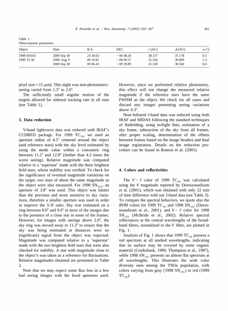
Table 1Observational parameters

Object Date R.A. DEC. r (AU) D (AU) a (8)

1998 SN165 2000 Sep 30 23 38.63 200 48.26 38.157 37.178 0.31999 TC36 2000 Aug 9 00 10.81 208 06.57 31.556 30.809 1.3

2000 Sep 30 00 06.43 208 39.89 31.538 30.560 0.4

pixel size515mm). This night was non-photometric- However, since we performed relative photometry,seeing varied from 1.30 to 2.60. this effect will not change the measured relative

The sufficiently small angular motion of the magnitude if the reference stars have the sametargets allowed for sidereal tracking rate in all runs FWHM as the object. We check for all cases and(see Table 1). discard any images presenting seeing variations

above 0.30.Near-Infrared J-band data was reduced using both

3 . Data reduction IRAF and MIDAS following the standard techniquesof flatfielding, using twilight flats, estimation of a

V-band lightcurve data was reduced with IRAF’s sky frame, subtraction of the sky from all frames,CCDRED package. For 1999 TC , we used an after proper scaling, determination of the offsets36

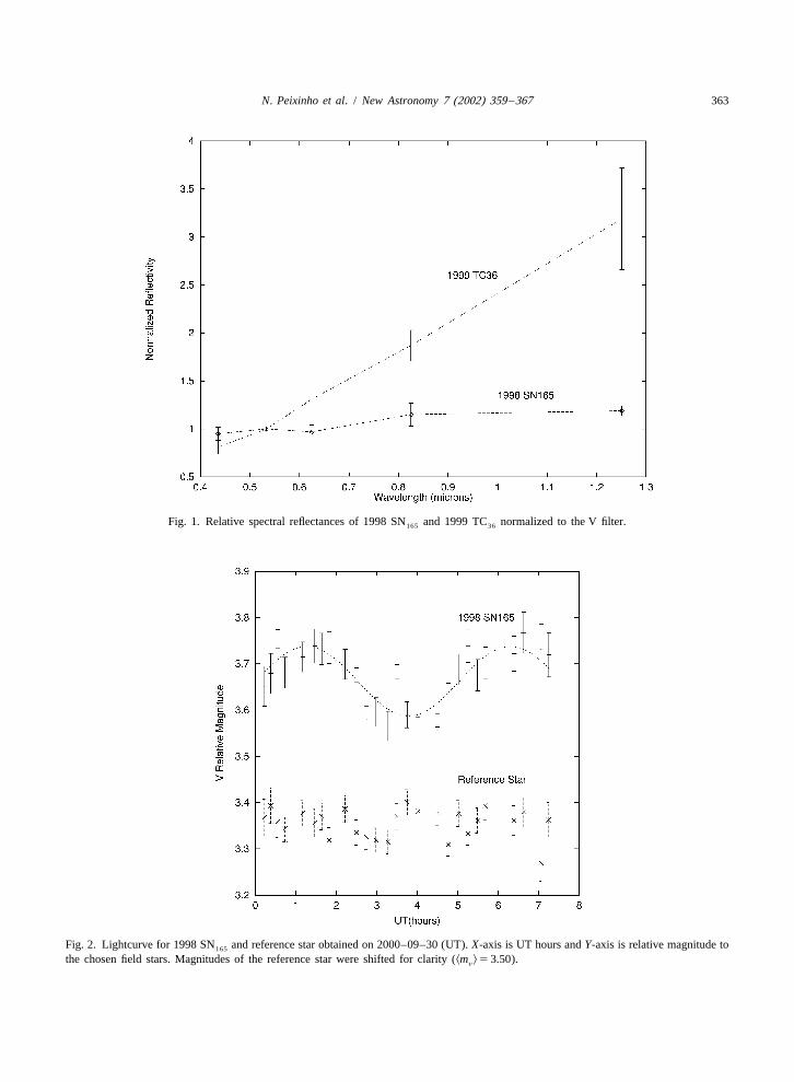
aperture radius of 4.50 centered around the object between frames based on the image headers and final(and reference stars) with the sky level estimated by image registration. Details on the reduction pro-using the mode value within a concentric ring cedure can be found in Romon et al. (2001).between 11.20 and 12.80 (farther than 4.3 times theworst seeing). Relative magnitude was computedrelative to a ‘superstar’ made with the three brightestfield stars, whose stability was verified. To check for 4 . Colors and reflectivitiesthe significance of eventual magnitude variations onthe target, two stars of about the same magnitude as TheV2 J color of 1999 TC was calculated36

the object were also measured. For 1998 SN , an using the V magnitude reported by Doressoundiram165

aperture of 3.80 was used. This object was fainter et al. (2001), which was obtained with only 22 minthan the previous and more sensitive to sky varia- of time difference with our J-band data (see Table 3).tions, therefore a smaller aperture was used in order To compare the spectral behaviors, we quote also theto improve theS/N ratio. Sky was estimated on a BVRI colors for 1999 TC and 1998 SN (Dores-36 165

ring between 8.00 and 9.60 in most of the images due soundiram et al., 2001), andV2 J color for 1998to the presence of a close star in some of the frames. SN (McBride et al., 2002). Relative spectral165

However, for images with seeings above 2.00, the reflectances at the central wavelengths of the broad-sky ring was moved away to 11.20 to ensure that the band filters, normalized to the V filter, are plotted insky was being estimated at distances were no Fig. 1.(significant) signal from the object was expected. Analysis of Fig. 1 shows that 1999 TC possess a36

Magnitude was computed relative to a ‘superstar’ red spectrum at all studied wavelengths, indicatingmade with the two brightest field stars that were also that its surface may be covered by some organicchecked for stability. A star with magnitude close to material (Cruikshank, 1989; Thompson et al., 1987),the object’s was taken as a reference for fluctuations. while 1998 SN presents an almost flat spectrum at165

Relative magnitudes obtained are presented in Table all wavelengths. This illustrates the wide color2. diversity seen among the TNOs population, with

Note that we may expect some flux loss in a few colors varying from gray (1998 SN ) to red (1999165

bad seeing images with the fixed apertures used. TC ).36

362 N. Peixinho et al. / New Astronomy7 (2002) 359–367

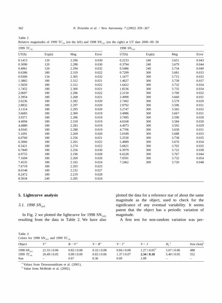
Table 2Relative magnitudes of 1999 TC (on the left) and 1998 SN (on the right) at UT date 2000–09–3036 165

1999 TC 1998 SN36 165

UT(h) Exp(s) Mag Error UT(h) Exp(s) Mag Error

0.1413 120 2.296 0.030 0.2233 240 3.651 0.0430.3090 120 2.288 0.030 0.3794 240 3.679 0.0440.4961 120 2.294 0.032 0.5486 240 3.734 0.0400.6386 180 2.319 0.022 0.7299 300 3.681 0.0330.9300 134 2.305 0.032 1.1677 300 3.715 0.0321.3865 180 2.312 0.021 1.4627 300 3.739 0.0371.5659 180 2.312 0.022 1.6422 300 3.732 0.0341.7452 180 2.300 0.021 1.8236 300 3.735 0.0342.0697 180 2.286 0.022 2.2150 300 3.700 0.0322.3954 180 2.268 0.021 2.4990 300 3.660 0.0312.6236 180 2.282 0.020 2.7492 300 3.579 0.0292.8832 180 2.297 0.020 2.9792 300 3.596 0.0313.1314 180 2.295 0.020 3.2747 300 3.565 0.0323.6683 180 2.300 0.019 3.4986 300 3.667 0.0313.9371 180 2.286 0.019 3.7495 300 3.590 0.0284.4094 180 2.318 0.019 4.0168 300 3.584 0.0304.6880 180 2.283 0.019 4.4973 300 3.592 0.0294.9345 180 2.288 0.019 4.7706 300 3.658 0.0315.1691 180 2.269 0.020 5.0189 300 3.688 0.0336.0760 180 2.256 0.021 5.2530 300 3.738 0.0356.3066 180 2.265 0.022 5.4889 300 3.676 0.0346.5421 180 2.274 0.022 5.6821 300 3.702 0.0356.7849 180 2.256 0.030 6.3979 300 3.722 0.0386.9755 180 2.196 0.028 6.6228 300 3.767 0.0447.1694 180 2.269 0.026 7.0591 300 3.732 0.0547.4535 180 2.165 0.024 7.2462 300 3.720 0.0487.6719 180 2.203 0.0258.0148 180 2.232 0.0278.2472 180 2.219 0.0288.5034 240 2.205 0.024

5 . Lightcurve analysis plotted the data for a reference star of about the samemagnitude as the object, used to check for the

5 .1. 1998SN significance of any eventual variability. It seems165

patent that the object has a periodic variation ofIn Fig. 2 we plotted the lightcurve for 1998 SN magnitude.165

resulting from the data in Table 2. We have also A first test for non-random variation was per-

Table 3Colors for 1998 SN and 1999 TC165 36

a a a a a aObject V B2V V2R V2 I V2 J H Size (km)V

b1998SN 21.5560.06 0.8260.08 0.3360.08 0.8460.08 1.2760.05 5.6760.06 488165

1999 TC 20.4960.05 0.9960.09 0.6560.06 1.3760.07 2.3460.18 5.4060.05 55236

Sun – 0.67 0.36 0.69 1.08 – –a Values from Doressoundiram et al. (2001).b Value from McBride et al. (2002).

N. Peixinho et al. / New Astronomy7 (2002) 359–367 363

Fig. 1. Relative spectral reflectances of 1998 SN and 1999 TC normalized to the V filter.165 36

Fig. 2. Lightcurve for 1998 SN and reference star obtained on 2000–09–30 (UT).X-axis is UT hours andY-axis is relative magnitude to165

the chosen field stars. Magnitudes of the reference star were shifted for clarity (km l53.50).v

364 N. Peixinho et al. / New Astronomy7 (2002) 359–367

21formed with the Chi-Square Test, in which thenull the frequencyf 50.199 h with a power of 8.28hypothesis is: there is no non-random variation (Fig. 3).(Collander-Brown et al., 1999). The weighted mean To check for the level of significance in the

¯magnitude is calculated for the object (x ) and then estimated period, we carried out a Monte-Carlow

the Chi-Square: simulation. Holding fixed the number of data-points,their time locationst and the corresponding errorsi2n ¯(x 2 x ) s , 10,000 random data-sets were constructed. Eachi w2 i]]]x 5O 2 randomx ; x(t ) was generated following a gaussians i ii51 idistribution of standard deviations . Applying thei

where x are the relative magnitude values,s the Lomb–Scargle periodogram to each one of thesei i

corresponding errors andn the number of data- random data-sets, we may estimate the probability ofpoints. Assuming that the errors are gaussian, and our detected frequency being due to noise—thefalsethat n is a large number, the mean limiting dis- period probability (P ). With only four events withf

2 2tribution is kxl 5n2 1 and the variance iss 5 higher powers than 8.28 we have aP 5 0.04%, thatf

2(n2 1). For 1998 SN and using a 26 data-point is, a significance levelof 99.96%.1652 21sample, we obtainedx 5 79.96, which is 7.8s (s 5 By fitting a sine-wave off 5 0.199h to the data

27.07) above the meankxl 5 25. Since the result is with the Levenberg–Marquardt algorithm, we de-larger than 3s, we have a significant rejection of the termine the magnitude variation, i.e., peak to peaknull hypothesis. amplitude, ofDm50.151. After subtracting this

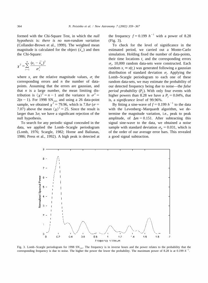
To search for any periodic signal concealed in the signal sine-wave to the data, we obtained a noisedata, we applied the Lomb–Scargle periodogram sample with standard deviations 5 0.031, which isN

(Lomb, 1976; Scargle, 1982; Horne and Baliunas, of the order of our average error bars. This revealed1986; Press et al., 1992). A high peak is detected at a good signal subtraction.

Fig. 3. Lomb–Scargle periodogram for 1998 SN . The frequency is in inverse hours and the power relates to the probability that the16521corresponding frequency is due to noise. The higher the power the lower the probability. The maximum power of 8.28 is at 0.199h .

N. Peixinho et al. / New Astronomy 7 (2002) 359–367 365

To determine the error in the frequency, we also cannot be ruled out, in which case the rotationalperformed a Monte-Carlo simulation. Analogously to period would be half of the computed value above.the previous simulation, we generated 1000 data-sets, In order to check for the real variability of thenow adding the gaussian noise to the signal obtained object’s magnitude, we performed also the Chi-

2from the fitted sine wave and applying the Lomb– Square test on a reference star. Ax 527.00 was2Periodogram to each set. The resulting distribution found, which is only 0.28s above thekx l, well

had a mean value ofk f l5 0.198 and a standard within the 3s bounds of the null hypothesis. Thedeviation of s 50.016. Therefore, our detected results assure the stability of the relative photometryf

frequency is: and thus confirm that the object’s variability is real.Also, the Lomb–Scargel periodogram applied to the

21f 50.19960.016h reference star did not reveal any significant periodicsignal.

The error in the amplitude is estimated by taking5 .2. 1999TCthe two extreme values (amplitude plus or minus its 36

error from the fit), resulting from fitting the sine-We observed 1999 TC over 8.362 h and nowave with f 5 0.1991s and f 5 0.1992s . We get 36f f

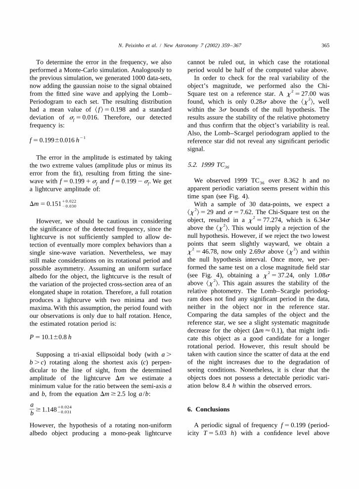
apparent periodic variation seems present within thisa lightcurve amplitude of:time span (see Fig. 4).

10.022Dm 5 0.151 With a sample of 30 data-points, we expect a20.030

2kx l5 29 ands 5 7.62. The Chi-Square test on the2object, resulted in ax 5 77.274, which is 6.34sHowever, we should be cautious in considering

2above thekx l. This would imply a rejection of thethe significance of the detected frequency, since thenull hypothesis. However, if we reject the two lowestlightcurve is not sufficiently sampled to allow de-points that seem slightly wayward, we obtain atection of eventually more complex behaviors than a

2 2x 5 46.78, now only 2.69s abovekx l and withinsingle sine-wave variation. Nevertheless, we maythe null hypothesis interval. Once more, we per-still make considerations on its rotational period andformed the same test on a close magnitude field starpossible asymmetry. Assuming an uniform surface

2(see Fig. 4), obtaining ax 5 37.24, only 1.08salbedo for the object, the lightcurve is the result of2above kx l. This again assures the stability of thethe variation of the projected cross-section area of an

relative photometry. The Lomb–Scargle periodog-elongated shape in rotation. Therefore, a full rotationram does not find any significant period in the data,produces a lightcurve with two minima and twoneither in the object nor in the reference star.maxima. With this assumption, the period found withComparing the data samples of the object and theour observations is only due to half rotation. Hence,reference star, we see a slight systematic magnitudethe estimated rotation period is:decrease for the object (Dm ¯0.1), that might indi-

P 5 10.160.8h cate this object as a good candidate for a longerrotational period. However, this result should betaken with caution since the scatter of data at the endSupposing a tri-axial ellipsoidal body (witha .

of the night increases due to the degradation ofb . c) rotating along the shortest axis (c) perpen-seeing conditions. Nonetheless, it is clear that thedicular to the line of sight, from the determinedobjects does not possess a detectable periodic vari-amplitude of the lightcurveDm we estimate aation below 8.4h within the observed errors.minimum value for the ratio between the semi-axisa

and b, from the equationDm $ 2.5 log a /b:

a 10.024] 6 . Conclusions$ 1.14820.031b

A periodic signal of frequencyf 5 0.199 (period-However, the hypothesis of a rotating non-uniformicity T 5 5.03 h) with a confidence level abovealbedo object producing a mono-peak lightcurve

366 N. Peixinho et al. / New Astronomy 7 (2002) 359–367

Fig. 4. Lightcurve for 1999 TC and reference star obtained on the 2000–09–30.X-axis is in UT hours andY-axis in relative magnitude to36

the chosen field stars. Magnitudes of the reference star were shifted for clarity (km l52.32).v

99.9% is present on our V-band lightcurve of 1998 by the grant (SFRH/BD/1094/2000) and projectSN with a peak-to-peak magnitude variation of (ESO/PRO/40158/2000) from the FCT (Portugal).165

Dm 5 0.15. A possible rotational period ofP 5

10.160.8 h and asymmetry ratio ofa /b $1.15 areestimated. This rotational period is to be taken with R eferencescaution and should be confirmed with better sampledobservations. For 1999 TC , we do not detect any Barucci, M.A. et al., 2001. A&A 371, 1150.36

periodic variation over our 8.4h time-span within Boehnhardt, H. et al., 2001. A&A 378, 653.Brown, W.R., Luu, J.X., 1997. Icarus 100, 288.the uncertainties. If 1999 TC has a detectable36Brown, M.E., Trujillo, C.A., 2002. IAUC 7807.rotational period it warrants longer observations.Buie, M.J., Bus, S.J., 1992. Icarus 100, 223.

From the relative reflectance spectra obtained with Bus, S.J. et al., 1989. Icarus 77, 223.the BVRIJ colors, of 1999 TC we see that it Collander-Brown, S.J. et al., 1999. MNRAS 308, 588.36

possesses a red spectrum, probably resulting from aCruikshank, D., 1989. AdSpR 6, 65.Davies, J.K. et al., 2000. Icarus 146, 253.cover of organic material on its surface.Doressoundiram, A. et al., 2001. Icarus 154, 277.Doressoundiram, A. et al., 2002. AJ (in press).Duncan, M.J., Quinn, T., Tremaine, S., 1988. ApJ 328, L69.Edgeworth, K., 1943. J. Br. Astron. Soc. 53, 181.

A cknowledgements Edgeworth, K., 1949. MNRAS 109, 600.Farnham, T.L., 2001. IAUC 7583.

´Gutierrez, P. et al., 2001. A&A 371, L14.The authors most kindly thank text revision fromHainaut, O.R., Delsanti, A.C., 2002. A&A (in press).

M.E. Filho (Kapteyn Institute) and constructive Hainaut, O.R. et al., 2000. A&A 356, 1076.comments from M. Roos-Serote (OAL/CAAUL) Horne, J.H., Baliunas, S.L., 1986. ApJ 302, 757.and M.A. Barucci (Observatory Paris). N.P. is funded Jewitt, D., Luu, J.X., 1993. Nature 362, 730.

N. Peixinho et al. / New Astronomy 7 (2002) 359–367 367

Jewitt, D., Sheppard, S.S., 2002. AJ 123, 2110. Romanishin, W., Tegler, S.C., 1999. Nature 398, 129.Kuiper, G.P., 1951. On the Origin of the Solar System, in: Romanishin, W. et al., 2001. Proc. Nat. Astron. Soc. 98, 11863.

Astrophysics, Hynek, J.A. (Ed.), McGraw-Hill, New York, p. Romon, J. et al., 2001. A&A 376, 310.357. Scargle, J.D., 1982. ApJ 263, 835.

Lomb, N.R., 1976. Ap&SS 39, 447. Tegler, S.C., Romanishin, W., 2000. Nature 407, 979.McBride, N. et al., 2002. Icarus (submitted). Thompson, W.R. et al., 1987. JGR 92, 14933.Ortiz, J.L. et al., 2002. A&A 388, 661. Trujillo, C.A., Brown, M.E., 2002. IAUC 7787.Press, W.H. et al., 1992. In: Numerical Recipes in Fortran: The Art

of Scientific Computing, 2nd Edition. Cambridge Univ. Press,London, p. 569.