Embed Size (px)
Citation preview
1
Vision for Industry
Cognex Corporation
Project Group Members:
Britt Fisher [email protected]
Bryan McCalister [email protected]
Chris Nelson [email protected]
Ray O’Connor [email protected]
Taylor Pettigrew [email protected]
2
Table of Contents:
Executive Summary 8 Business and Industry Analysis 10
Company Overview 17
Industry Overview 19
Five Forces Model 24
Rivalry of Existing Firms 25
Industry Growth Rate 25
Concentration of Competitors 27
Differentiation 29
Learning Economies 29
Excess capacity 30
Exit Barriers 31
Conclusion 31
Threat of New Entrants 31
Economies of Scale 32
First Mover Advantage 34
Legal Barriers 35
Conclusion 36
Threat of Substitute Products 37
Customers’ Willingness to Switch 38
Conclusion 39
Bargaining Power of Customers 39
3
Price sensitivity of Customer 40
Relative Bargaining Power-Customer 40
Customer Switching Cost 41
Conclusion 42
Bargaining Power of Suppliers 42
Price sensitivity of Supplier 43
Relative Bargaining Power-Supplier 43
Conclusion 43
Industry Analysis 44
Superior Product Quality 44
Superior Product Variety 45
Superior Customer Service 46
R&D 47
Investment in Brand Image 48
Value Creation Analysis 49
Superior Customer Service 49
Superior Product Variety 53
R&D 53
Superior Product Quality 54
4
Conclusion 56
Formal Accounting Analysis 56
Key Accounting Policies 57
Goodwill 58
Research and Development 60
Foreign Currency 62
Accounting Flexibility 65
Goodwill 66
Research and Development 68
Foreign Currency 69
Evaluate Accounting Strategy 70
Goodwill 70
Research and Development 72
Foreign Currency 74
Qualitative Disclosure 81
Goodwill 81
Research and Development 83
Foreign Currency 83
Conclusion 85
Quantitative Analysis 85
Revenue Manipulation Diagnostics 86
Net sales/cash from sales 86
Net sales/accounts receivable 88
Net sales/ inventory 90
5
Net sales/warranty expense 92
Conclusion 94
Expense Manipulation Diagnostics 95
Cash flow from operations/operating income 95
Cash flow from operations/net operating assets 97
Asset turnover 99
Total Accruals/sales 101
Potential Red Flags/Undo Accounting Distortions 103
Research and Development 103
Goodwill 104
Restated Income Statement 108
Restated Balance Sheet 109
Financial Analysis, Forecasting Financials, and Cost of Capital Estimation 110
Financial Analysis 110
Liquidity Ratio Analysis 111
Current Ratio 111
Quick Asset Ratio 113 Inventory Turnover 115
Days Supply Inventory 116
Accounts receivable turnover 118
Days Sales Outstanding 119
6
Cash to Cash Cycle 122
Working Capital Turnover 123
Conclusion 125
Profitability Ratio Analysis 126
Gross Profit Margin 126
Operating expense ratio 128
Operating profit margin 130
Net Profit Margin 132
Asset Turnover 134
ROA 136
ROE 138
Conclusion 140
Growth rate Ratios 140
Internal growth rate 141
Sustainable growth rate 142
Conclusion 144
Capital Structure Analysis 144
Debt to Equity ratio 145
Times interest Earned 147
7
Debt Service margin 148
Z-score 149
Conclusion 151
Financial Statement Forcasting 152
Income Statement 152 Income Statement (Restated) 157 Balance Sheet 159 Balance Sheet (Restated) 162 Statement of Cash Flows 164 Statement of Cash Flows (Restated) 167
Estimating Cost of Capital
Cost of Debt 169
Cost of Equity 170
Size Adjusted 173
Alternative Cost of Equity 173
Weighted average cost of capital 174
Method of Comparables 175
P/E Trailing 175
P/E Forecast 177
P/B 178
PEG 179
P/EBITDA 180
8
EV/EBITDA 181
P/FCF 182
D/P 184
Conclusion 185
Intrinsic Valuation Models 186
Discounted Dividends Model 186
Residual Income Model 188
Residual Income Model Restated 190
Discounted Free Cash Flows Model 190
Discounted Free Cash Flows Model Restated 193
AEG Model 193
Long Run Residual Income Model 196
Long Run Residual Income Model Restated 198
Analyst Recommendation 199
Appendices 201
References 237
9
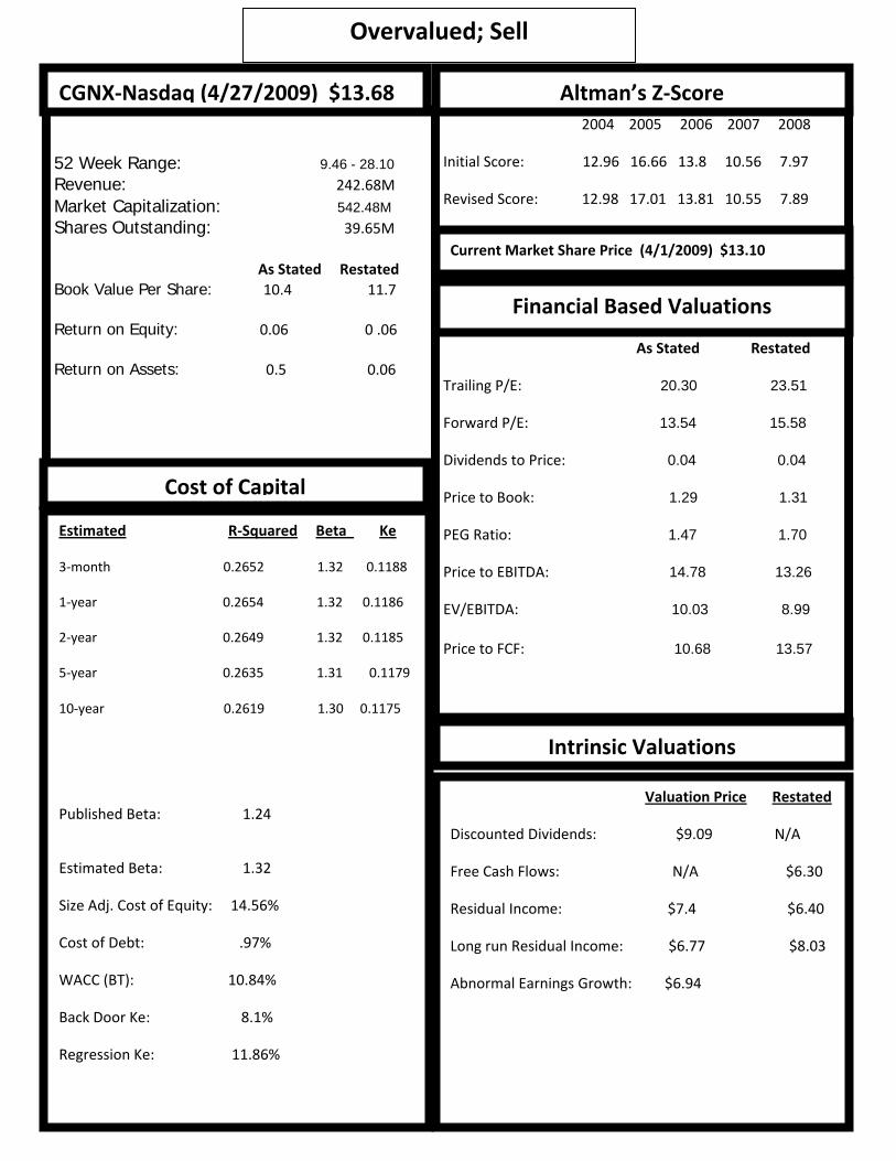
52 Week Range: 9.46 - 28.10 Revenue: 242.68M Market Capitalization: 542.48M Shares Outstanding: 39.65M
As Stated Restated Book Value Per Share: 10.4 11.7 Return on Equity: 0.06 0 .06 Return on Assets: 0.5 0.06
2004 2005 2006 2007 2008
Initial Score: 12.96 16.66 13.8 10.56 7.97
Revised Score: 12.98 17.01 13.81 10.55 7.89
As Stated Restated
Trailing P/E: 20.30 23.51
Forward P/E: 13.54 15.58
Dividends to Price: 0.04 0.04
Price to Book: 1.29 1.31
PEG Ratio: 1.47 1.70
Price to EBITDA: 14.78 13.26
EV/EBITDA: 10.03 8.99 Price to FCF: 10.68 13.57
CGNX‐Nasdaq (4/27/2009) $13.68 Altman’s Z‐Score
Current Market Share Price (4/1/2009) $13.10
Financial Based Valuations
Estimated R‐Squared Beta Ke
3‐month 0.2652 1.32 0.1188
1‐year 0.2654 1.32 0.1186
2‐year 0.2649 1.32 0.1185
5‐year 0.2635 1.31 0.1179
10‐year 0.2619 1.30 0.1175
Published Beta: 1.24
Estimated Beta: 1.32
Size Adj. Cost of Equity: 14.56%
Cost of Debt: .97%
WACC (BT): 10.84%
Back Door Ke: 8.1%
Regression Ke: 11.86%
Cost of Capital
Intrinsic Valuations
Valuation Price Restated
Discounted Dividends: $9.09 N/A
Free Cash Flows: N/A $6.30
Residual Income: $7.4 $6.40
Long run Residual Income: $6.77 $8.03
Abnormal Earnings Growth: $6.94
Overvalued; Sell
10
11
Executive Summary
Industry Analysis
Created in 1981 Cognex is the largest provider in machine vision software, vision
systems, vision sensors, and surface inspection systems utilized in manufacturing
automation. The company is headquartered in Natick, Massachusetts with offices in
twenty countries including North America, Japan, Latin America, Asia and Europe.
Cognex has the largest global presence of any firm in the industry. In the machine
vision industry Cognex competes directly with KLA-Tencor, Perceptron, Orbotech, and
Electro Scientific Industries Inc (ESIO). Each of the firms are fairly different in terms of
geographic location, primary business focus, and competitive advantages.
Since the firms in this industry are dealing with a global client base, they rely
heavily on product differentiation in order to stay ahead of their competitors. The only
way to stay ahead of the curve in the industry is to be at the forefront of technical
innovation. Dealing with a highly technical product, the firms must all invest large
Competitive force Degree of Competition
Rivalry among existing firms High
Threats of new entrants Moderate
Threat of substitute products High
Bargaining power of customers Low
Bargaining power of suppliers High
12
amounts of money in research and development in order to remain differentiated
against their competitors. Due to the continuous efforts required by the firms to stay
ahead in this industry the rivalry among existing firms is high. This particular technical
field presents the opportunity for abnormal positive earnings. The industry has low
barriers to entry; however, success beyond the entry phase is very difficult. The high
level of difficulty to be successful past the initiation stages in this industry creates only a
moderate threat of new entrants. One of the greatest threats in this industry is the
threat of substitute products. When dealing with a technically advanced product base,
there is always a possibility of a substitute product. Various methods of reverse
engineering, and rapid product development create threats to a company’s level of
innovation. Performance then becomes the leading factor in preventing product
replacement by competing firms. The performance characteristics of the firm’s product
are what prevent the competitors from taking their market share. This high level
performance competition results in a high threat of substitute products. Given that the
products in this industry are relatively differentiated from one another, the customer
does not posses a large amount of bargaining power in this relationship. If the
customer wants a particular product from a firm in this industry they have little power
over the determination of the price levels. Ultimately the bargaining power of customers
is low in this industry. Conversely the overall bargaining power of suppliers is high in
this sector. The companies have products that the customers need in order to run their
operations. This gives the suppliers an upper hand in determining price levels and
quantity to be supplied. The suppliers in this industry invest large amounts of capital
13
into research and development, and for this reason they have a vast amount of control
over the bargaining power.
Accounting Analysis
To get a true picture of a firm and its operations, it is necessary to study its
financial records and disclosure policies. GAAP requires a minimum level of disclosure
for all firms, which aims to prevent misleading the public. Although this requires
companies to state details about their operations, it leaves room for managers to over or
understate specific line items in an attempt to make the company look more profitable to
investors. A firm with detailed disclosure within their 10-K will look trustworthy and
credible in its operations. However, firms providing only a minimum level of disclosure
present concerns for those wanting to invest. It is important to analyze details within the
accounting disclosure and identify “red flags” if necessary.
The first step in accounting analysis is to identify key success factors. Some key
success factors for Cognex and its industry are research and development, product
differentiation, superior quality, global distribution and value creation for the customer.
To properly value the firm, these key success factors must be linked to the key
accounting policies. The key accounting policies that most directly affect Cognex’s key
success factors include research and development, goodwill and foreign currency risk.
The amount of detail in the disclosure of the mentioned key success factors will either
support the financial statements or expose distortions.
Goodwill is a major operation of many companies and can be manipulated on the
balance sheet. Before 2005 Cognex had a relatively small amount of goodwill on its
14
books, but after several acquisitions in 2005 and 2006 the goodwill account amounted
to almost 15% of total assets. Moderate levels of disclosure only tell part of the story.
The aggressive accounting for goodwill needed to be further analyzed to get a truly
transparent picture of how goodwill is accounted for. This is evidence of a type 2
accounting distortion and is identified by a “red flag”. In order to present a more
reasonable estimate of goodwill, 20% of the account was amortized. This decreased the
value of assets and added an amortization expense to the income statement, helping to
present a better overall picture of firm operations.
The research and development account was also identified as a type 2
accounting distortion and needed to be altered. Cognex does not provide much
disclosure within research and development, signaling another red flag. A similar
approach was used to reduce the enormous R&D expenses piling up on the income
statement; 20% of R&D was capitalized to reduce expenses to a reasonable amount.
Disclosure of foreign currency risk is moderate. The company 10-K states that it
uses financial instruments to hedge against this risk, but does not go into detail about
the measures used. It does state that it hedges using forward contracts among other
instruments. This type 1 accounting distortion was further examined in order to see
exactly how foreign currency risk affected Cognex. Overall Cognex moderate disclosure
with goodwill and R&D, but the aggressive accounting strategy showed that several line
items needed to be restated.

15
Financial Analysis, Cost of Capital Estimation, and Forecasting
In order to thoroughly evaluate a firm, it is necessary to go through extensive
financial analysis including ratio analysis, estimating the cost of capital, and forecasting
financials. Examining each of these aspects of the firms will provide a more in-depth
view of how well the firm is functions on an annual basis.
Firms and analysts alike often times use ratios to draw simplistic comparisons
between their performance and the performance of their competitors. The primary
types of ratio analysis classifications are liquidity analysis, profitability analysis, and
capital structure analysis. Liquidity ratios are used to explain how easily a firm can pay
its short term debt obligations. These ratios are used to discuss the overall financial
health of the firms. Analysts may use the liquidity ratios to develop a general idea as to
the level of risk within a particular firm. As a broad generalization the higher the ratios
the more safety a firm exhibits. Cognex was able to maintain average to above average
ratios throughout the liquidity analysis section. The company was also able to produce
industry leading numbers in the working capital turnover ratio. Profitability ratios explain
how successfully a firm can generate revenues in excess of their expenses. The
profitability ratios will allow analysts to understand what expenses are incurred from the
general operations as well as the revenues produced to cover those expenses. Cognex
performed exceptional with the analysis of the profitability ratios. The firm was able to
display consistent industry leading results in most of the ratio categories. The ratios in
which they did not lead to industry were still consistent and promising providing no
cause for concern. The final classification of financial ratio analysis is capital structure
ratios. Capital structure ratios are used to help understand the overall structure of
16
leverage for each firm as well as to aide in determining credit ratings. A firm can
finance its assets by either utilizing debt financing or equity financing. Firms that rely
more heavily on equity financing are easily capable of paying off their liabilities and
interest as it becomes due. Companies that utilize more debt financing are seen as
higher risk endeavors. Several of the capital structure ratios are unable to be computed
consistently in this industry due to the trend of firms holding no long term debt. The
debt to equity ratio is the most useful ratio when dealing with the Scientific and
Technological Instruments industry. A lower ratio is favorable in this category
suggesting that a company is more dependent upon equity financing than debt
financing. Cognex was once again at the forefront of the industry with persistently low
and consistent ratio results.
In order to create an effective Prospective analysis we needed to forecast the
income statement balance sheet, and stament of cash flows in both nominal and
restated terms. The most important forecast needed to determine our net income each
period ending was expected sales growth. We concluded that sales would continue to
rise in a cycle like pattern at 6% then effectively drop in year 2012. Cost of goods sold
remained at a steady retrospective average of 71% of revenue so we assumed this
could be applicable to future forecasts as well. Other forecast could be represented as
a % of sales to ultimately arrive at a forecasted net income. To connect the income
stamen to the balance sheet a return on assets average was used to forecast our total
assets through year 2019. Retained earnings can be forecasted through a net income
amount less forecasted dividends, and the net change in retained earrings was sued to
forecast our book value in equity. CFFO was forecasted as a % of OI for both restated
17
and nominal. We concluded that dividends were not a well forecasted as a function of
NI and created a growth that was more representative of past pay outs.
Using a CAPM method were r able to attain what we felt to be the most
reasonable estimate of Kd at 11.86, although we did calculate other estimates such as
the back door and size adjusted. Our estimate of Kd equated to .97 . Such a low
estimate is not out of the ordinary because of Cognex’s low amounts of reported long
term Liabilities. Next using estimates of Kd and Ke we were able to find our WACC at
10.84 before tax and 10.81 after tax.
Valuation
The last step in the equity valuation analysis is to estimate a current market
share price. We used several techniques to achieve this. First, we studied trends of
financial ratios through the method of comparables. This technique compares financial
ratios of companies with similar cash flow and business operation. The other valuation
method used involves intrinsic valuation models, a much more sophisticated approach.
It is almost impossible to predict current market price down to the penny, so we decided
to use a range of +/- 15% in share price to determine whether the firm is overvalued,
undervalued, or fairly valued.
We began the valuation analysis using the method of comparables. Competitor’s
ratios were averaged against Cognex’s to determine proper valuation. It is important to
exclude outliers when calculating industry averages, as these can adversely affect the
credibility of the conclusion. Of the 8 comparables used, 5 concluded Cognex is
18
overvalued, 2 concluded fairly valued, and one concluded undervalued. It is apparent
that through the method of comparables Cognex is determined to be overvalued.
The intrinsic valuation models offer a more accurate estimate of value because
they offer more insight into the detail of company operations, as opposed to industry
comparison. Data from our forecasted financial statements was discounted to get a
present value. We also used sensitivity analysis to see how different growth rates and
costs of capital affected current share price. We then determined if the firm was
overvalued, undervalued, or fairly valued based on a 15% margin of error. All of the
models conclude that the current market price of Cognex is overvalued. The only
drawback to the intrinsic models is that they rely on estimates, not concrete numbers.
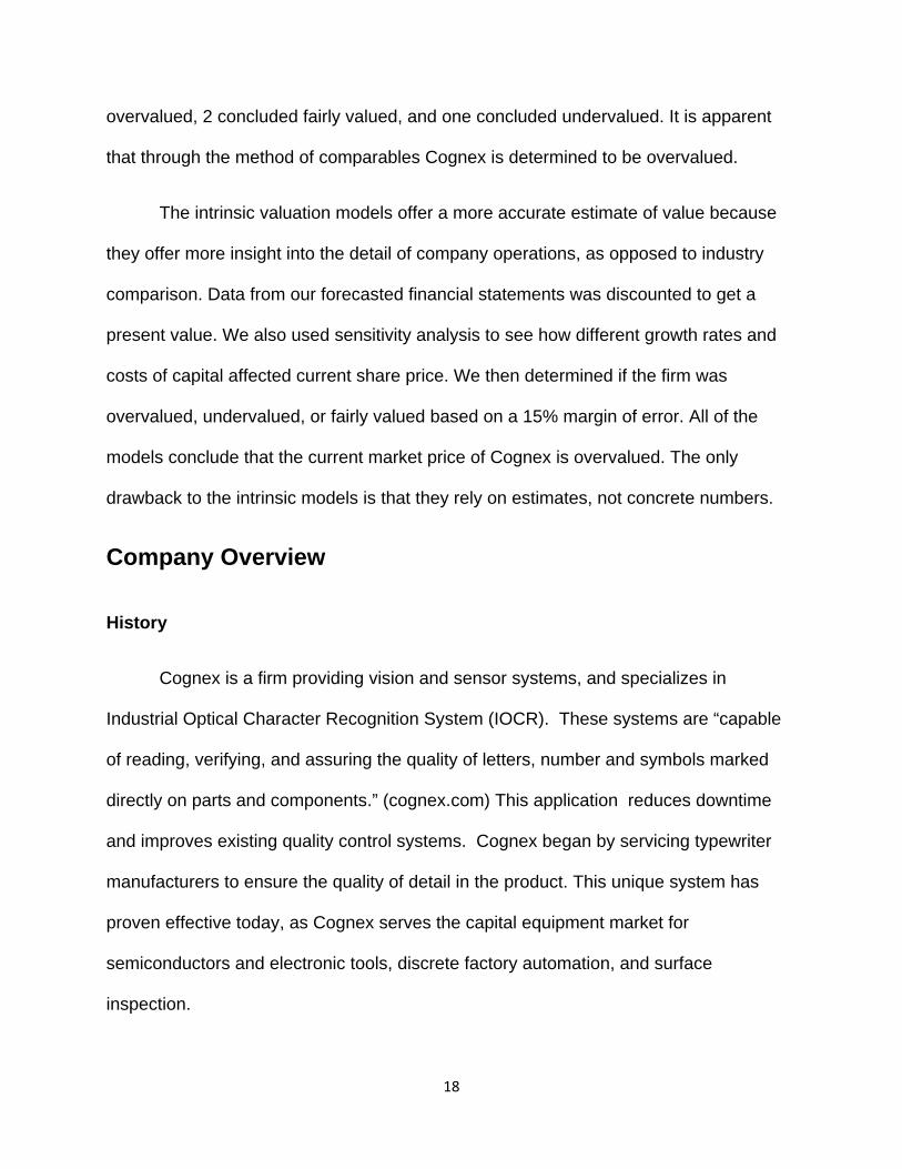
Company Overview
History
Cognex is a firm providing vision and sensor systems, and specializes in
Industrial Optical Character Recognition System (IOCR). These systems are “capable
of reading, verifying, and assuring the quality of letters, number and symbols marked
directly on parts and components.” (cognex.com) This application reduces downtime
and improves existing quality control systems. Cognex began by servicing typewriter
manufacturers to ensure the quality of detail in the product. This unique system has
proven effective today, as Cognex serves the capital equipment market for
semiconductors and electronic tools, discrete factory automation, and surface
inspection.
19
The two divisions Cognex operates in are: Modular Vision Systems (MVS), and
Surface Inspection Systems. The MVS segment uses a variety of handheld cameras
strategically placed along the assembly line or throughout the assembly process.
These cameras will then analyze the orientation, size, and appearance of the product.
The diagnostics are then transferred to an easy to use interface monitor. This vision
software allows a firm to analyze the efficiency of the assembly process and increases
the speed and precision of product defect detection. This is very important to a firm
mass producing products, in order to identify problems early. These processes help to
improve product quality, customer satisfaction, and maintain the brand image. This
division is responsible for 87% of total company revenue. (cognex 10-k)
The second segment Cognex operates in is the Web and Surface Inspection
System, which makes up 13% of sales. The Web and Surface Inspection systems and
the Smart View software uses cameras in addition to lighting and imaging software to
detect and classify defects in metals, paper, plastics, non-wovens, and glass
(cognex.com). This software allows firms to guarantee perfection on flat and irregular
surfaces. The optical lenses can be easily installed with little or no downtime. Cognex
customers are located in three markets: semiconductor and electronic capital
equipment, surface inspection, and discrete factory automation. (cognex 10-k)
Fundamentals
Research, development, and engineering (R,D, & E) is extremely important to
Cognex. It is important to improve existing products as well as develop new techniques
to improve product performance. Failure to develop new products and respond to
20
technological changes could affect Cognex adversely through loss of profit and market
share. Cognex currently invests 15% of sales in research, development and
engineering. This has allowed Cognex to develop several new products to help sustain
its market share.
Industry Overview
The industry in which Cognex operates is Scientific and Technical Instruments.
Cognex and its top competitors , KAL-Tencor, Orbotech, Perceptron, and Electro
Scientific Industries Inc. are companies classified under North American Industry
Classification as “Instruments and Related Products Manufacturing for Measuring,
Displaying, and Controlling Industrial Process Variables”(NAIC). Firms in this industry
design, manufacture, and market the technical tools that serve manufacturing
companies today. These products are used in process and control devices, precise
measurement and signal processing, and other technologically advanced machinery.
The industry has seen extensive growth as a result of a technology boom in the 1980’s.
Machine vision, wafer identification and surface inspection systems are three general
applications this industry specializes in. This industry is very cyclical in nature due to
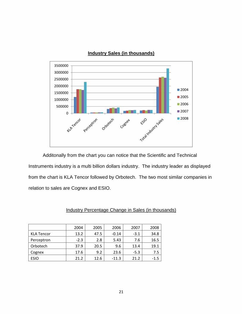
the heavy reliance on technological innovations and advancements. The chart below
demonstrates the size of each firm in the industry based on sales. It also demonstrates
the amount of the firm’s sales in comparison to the industries total sales.
21
Industry Sales (in thousands)
Additonally from the chart you can notice that the Scientific and Technical
Instruments industry is a multi billion dollars industry. The industry leader as displayed
from the chart is KLA Tencor followed by Orbotech. The two most similar companies in
relation to sales are Cognex and ESIO.
Industry Percentage Change in Sales (in thousands)
2004 2005 2006 2007 2008KLA Tencor 13.2 47.5 ‐0.14 ‐3.1 34.8Perceptron ‐2.3 2.8 5.43 7.6 16.5Orbotech 37.9 20.5 9.6 13.4 19.1Cognex 17.6 9.2 23.6 ‐5.3 7.5ESIO 21.2 12.6 ‐11.3 21.2 ‐1.5
0
500000
1000000
1500000
2000000
2500000
3000000
3500000
2004
2005
2006
2007
2008
22
From the chart above you can observe the cyclicality of the market. Every year one or
two firms excelled from the previous year while one or two others fell. This is due to
firm’s new innovations and technological advancements giving them a competitive
advantage.
Machine Vision
“Machine vision integrates image capture systems with digital input/output
devices and computer networks to control manufacturing equipment such as robotic
arms.” (machinevision.co.uk). Cognex, Perceptron, Orbotechm and ESIO mainly
participate in this industry. Machine vision equipment was first used in the early 1950’s
as a military application to research artificial intelligence. This technology proved itself to
be practical and effective, drawing some of the world’s highest profile institutions to
conduct further research. In the late 1960’s and into the 1970’s Massachusetts Institute
of Technology (MIT) developed the first machine vision application that would soon
prove to drive an entire industry. The competitors in this industry began pouring money
into Research and Development in an attempt to perfect machine vision processes and
develop new revenue streams. In the 1980’s it was apparent that firms applying
machine vision would become part of an extremely lucrative industry. Manufacturers
began installing applications involving industrial cameras to monitor and control
production operations. Many firms in the semiconductor industry were among those to
adopt the new technology, driving machine vision firms to continue expanding to service
23
new markets and increase market share. The 1990’s to current have been some of the
fastest growing years for this industry, as demand for automation and quality increase
consistently.
Wafer Identification
Many firms particularly KLA Tencor competes in this industry. KLA is heavily
impacted by the semiconductor industry. “KLA‐Tencor's primary market is the
semiconductor industry.” (KLA Tencor 10‐K) The increase in technology has lead to an
extensive demand for smaller, more powerful computer chips.
Semiconductors, small pieces that make up integrated circuits (IC’s), were some of the
components that felt this demand the most. As production increased, it became more
important to track and identify product defects. Systems were designed to take the small
semiconductors (also known as wafers) and scan each product into a computer system
for analysis.
Wafer identification systems read numbers and characters through bar codes.
This enables firms to track their products and ensure a timely production process. The
wafer ID systems use optical lenses and lasers to “see, read and record” wafers
throughout the production process.http://news.thomasnet.com/fullstory/460005
).“Integrated lensing and lighting capabilities provide flexibility required to read code
consistently throughout various stages of production that subject wafer to changes in
appearance, such as contrast and color modifications.”
(http://findarticles.com/p/articles/mi_m0EIN/is_2005_June_28/ai_n14701699)
24
Surface inspection systems
Surface inspection is the main industry Cognex, Peceptron, KLA Tecnor, ESIO,
and Orbotech mainly compete in. All of the firms inspect Surface inspection systems
scan products for constant quality control evaluation. These systems serve a wide
variety of firms including those who produce metals, paper, plastics, and non-wovens.
Lenses and 360 degree cameras are used to monitor and control the production
process the many products. It is imperative for these firms to identify defects in their
products before costly value-added processes are added to the production phase. This
is especially important for automobile manufacturers, one of the largest consumers of
surface inspection equipment.
Conclusion
The increasing availability of industrial systems stimulated the need for new
technology, pushing R&D efforts ever higher throughout the Scientific and Technical
Instruments industry. This new machinery thus increased quality control standards
across the world. Constant demand on improved production capacity and minimal
product defects has allowed manufacturing firms to purchase equipment to meet these
zero tolerance standards. It is important for firms in this industry to be aware of both
25
customer and supplier perspectives in order to stay afloat in a competitive market
(Frost). Although some markets (ie. Surface inspection equipment) show strength in the
near future, the industry as a whole cannot say the same. Technology related
purchases by firms increased consistently from 2002 through 2008; in 2008 technology
purchases by firms and governments increased by 8% (Forrester Research). However,
according to
Forrester Research, a drop of 3% in technology purchases is expected in 2009
(Forrester Research). Overall the industry has shown extensive growth in the past
decade, but companies that strive to continue their operations will depend on constant
investment in research and development (xbitlabs.com). (WSJ)
Five Forces Model
The five forces model allows a company to analyze what effects the individual
firm in relation to the industry. Using this model will allow the firm to better compete in
the industry. Additionally can establish the amount of success and profitability the firm
will realize. The model analyzes the following five issues: Rivalry among existing firms,
threat of new entrants, threat of substitute products, bargaining power of customers,
and bargaining power of suppliers. The first three of these forces are used to analyze
profits of an industry based on competition, while the latter two describe relationship of
power between input and output markets (suppliers and consumers). The model is
picture below:
26
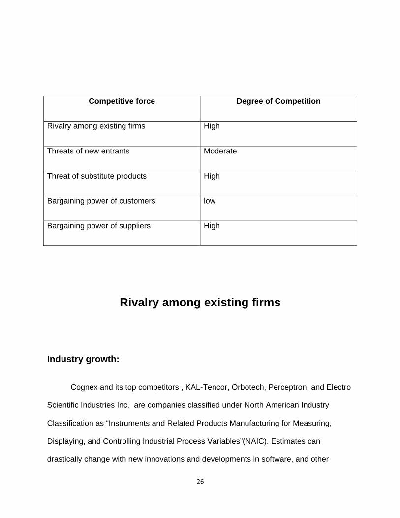
Competitive force Degree of Competition
Rivalry among existing firms High
Threats of new entrants Moderate
Threat of substitute products High
Bargaining power of customers low
Bargaining power of suppliers High
Rivalry among existing firms
Industry growth:
Cognex and its top competitors , KAL-Tencor, Orbotech, Perceptron, and Electro
Scientific Industries Inc. are companies classified under North American Industry
Classification as “Instruments and Related Products Manufacturing for Measuring,
Displaying, and Controlling Industrial Process Variables”(NAIC). Estimates can
drastically change with new innovations and developments in software, and other
27
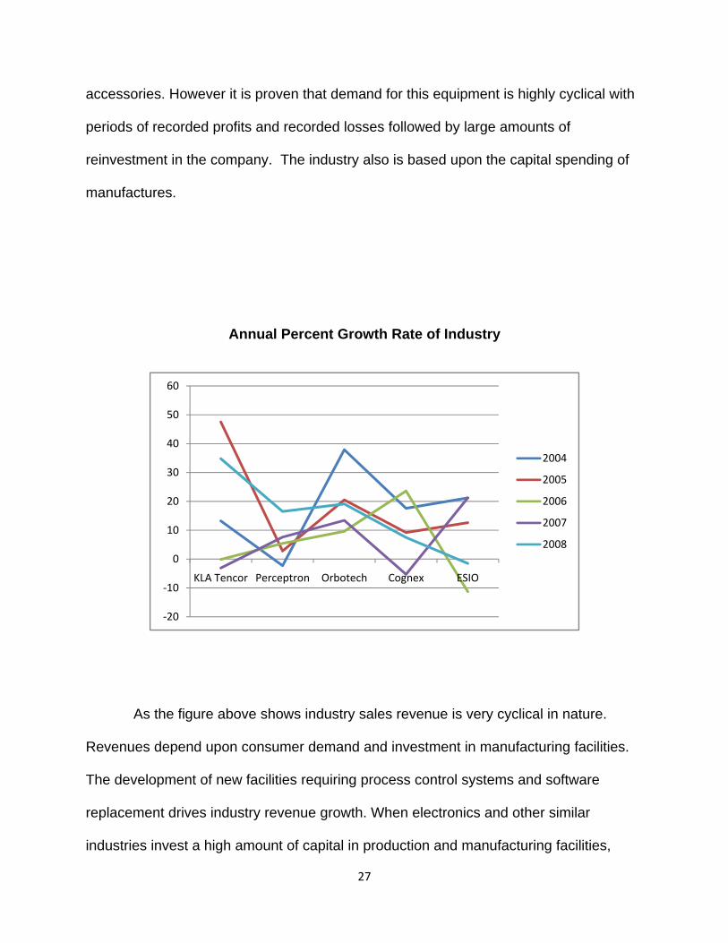
accessories. However it is proven that demand for this equipment is highly cyclical with
periods of recorded profits and recorded losses followed by large amounts of
reinvestment in the company. The industry also is based upon the capital spending of
manufactures.
Annual Percent Growth Rate of Industry
As the figure above shows industry sales revenue is very cyclical in nature.
Revenues depend upon consumer demand and investment in manufacturing facilities.
The development of new facilities requiring process control systems and software
replacement drives industry revenue growth. When electronics and other similar
industries invest a high amount of capital in production and manufacturing facilities,
‐20
‐10
0
10
20
30
40
50
60
KLA Tencor Perceptron Orbotech Cognex ESIO
2004
2005
2006
2007
2008
28
firms don’t need to capture others sales revenue to increase their market share. This
allows smaller firms to capture the industries excess capacity and grow within the
industry (Palepu & Healy).
Concentration :
Although a large number of firms compete in this industry, size does not ensure
dominance among firms with less than 50 million in annual revenue (Hardin).Firms with
smaller amounts of revenue are large in number and survey customers on a global
scale.
The smaller number of firms can be attributed to companies specializing their
efforts toward a specific industry. An industry with the vast amount of smaller
companies can still compete on prices and production level with larger firms because
their products and services can be tailored to specific manufacturing systems.
Particular company growth also depends to the extent that their firm specifically targets
markets. Large companies that compete in the industry may only have a fraction of
their sales revenue from inspection devices or controlling devices, while smaller firms
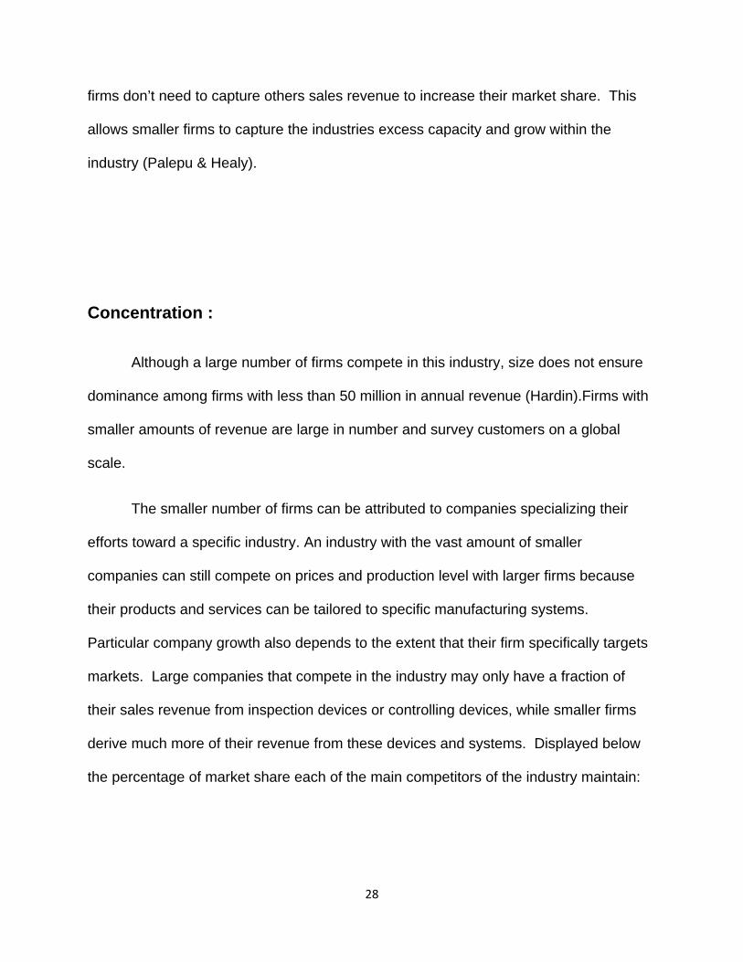
derive much more of their revenue from these devices and systems. Displayed below
the percentage of market share each of the main competitors of the industry maintain:
29
Annual Market Share
The graph illustrates KLA Tencor maintains the largest market share in the
industry. The chart also displays that no companies market share vastly changes from
year to year. This is attributed to the large amount of long term contracts this
companies and customers enter. KLA Tencor’s domination however does not allow
them to set prices. Due to the vast dependence of technology in the industry and the
fact thatother firms are always coming up with new and more advanced innovations it is
impossible to set prices for the market.
0
0.1
0.2
0.3
0.4
0.5
0.6
0.7
0.8
2004 2005 2006 2007 2008
KLA Tencor
Perceptron
Orbotech
Cognex
ESIO
30
Differentiation:
Firms can differentiate their products in a number of ways by focusing their
attention on specializing in the process control industry or by focusing on the products
themselves. Each instrument is fairly specialized which can help firms avoid head on
completion. Since most of the industry serve global end users, head on competition can
be somewhat avoided because their products and services are so specialized.
Learning economies
The process control industry has a steep learning curve and it is a necessity for
competing firms to spend time and money in research and development to create the
best product for their end user. Allowing the firm to capture a better hold of the market .
Companies in the industry spent on an industry average 2.3 billion in 2008 alone.
(Mergent online). Compared to the industry sales revenue firms will spend more on
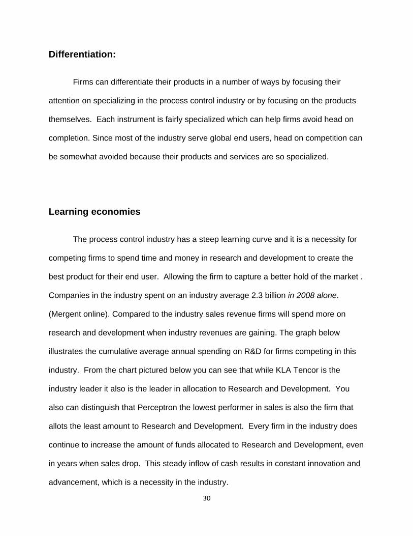
research and development when industry revenues are gaining. The graph below
illustrates the cumulative average annual spending on R&D for firms competing in this
industry. From the chart pictured below you can see that while KLA Tencor is the
industry leader it also is the leader in allocation to Research and Development. You
also can distinguish that Perceptron the lowest performer in sales is also the firm that
allots the least amount to Research and Development. Every firm in the industry does
continue to increase the amount of funds allocated to Research and Development, even
in years when sales drop. This steady inflow of cash results in constant innovation and
advancement, which is a necessity in the industry.
31
Average Annual Spending of R&D
Excess capacity
A large part of the demand for scientific and technical instrument industry comes
from a firm’s initial investment in manufacturing facilities. Firms may contribute a large
portion of their revenue from a specific industry such as automotive or concentrated
orange juice production. The scientific and technical instrument industry is constantly
evolving technologically. Due to the fact that advancements are highly desired, excess
capacity has yet to affect prices throughout the industry.
0
0.1
0.2
0.3
0.4
0.5
0.6
KLA Tencor Perceptron Orbotech Cognex ESIO
2004
2005
2006
2007
2008
32
Exit Barriers
The scientific and technical instrument industry requires highly specialized
assets, resulting in high exit barriers. As a result specialized assets being highly ill-
liquid, it deters many firms from leaving the industry.
Conclusion
The rivalry among existing firms is highly competitive. The competitive nature of
the industry can be based upon the fact it is highly based upon differentiation. The
reliance on differentiation makes switching costs high, as well as exit barriers. The
industry is also highly competitive due to the fact of the high growth rate it has
experienced in the past several years. As the industry continues to grow, the
innovations and advancements do as well giving the industry even more growth
potential.
The Threat of New Entrants
The scientific and technical instruments market offers a great possibility for
earning abnormal profits. There are few barriers to enter into the market increasing the
competition between firms. The threat of new entrants in the market is relatively
moderate. However entering the market and being successful in the market do not go
hand in hand. Some of the factors that will determine whether a firm will enter the
industry and the amount they will invest are economies of scale, first mover advantage,
33
and access to channels of distribution and relationships, and the legal barriers. Upon
analyzing these factors the threat of new entrants in moderate throughout the industry.
Economies of Scale
In the scientific and technical instruments market there are small economies of
scale. The industry does require a large amount of capital invested in PPE and
Research and Development initially. This does not alleviate all the danger of entering
a new market however, “either way new entrants will at least initially suffer from a cost
disadvantage in competing with existing firms” (Palepu & Healy). However a large
amount of current assets gives firms a greater advantage to increase their market
share. The chart displayed below presents the total assets for Cognex and its top three
competitors for the previous five years
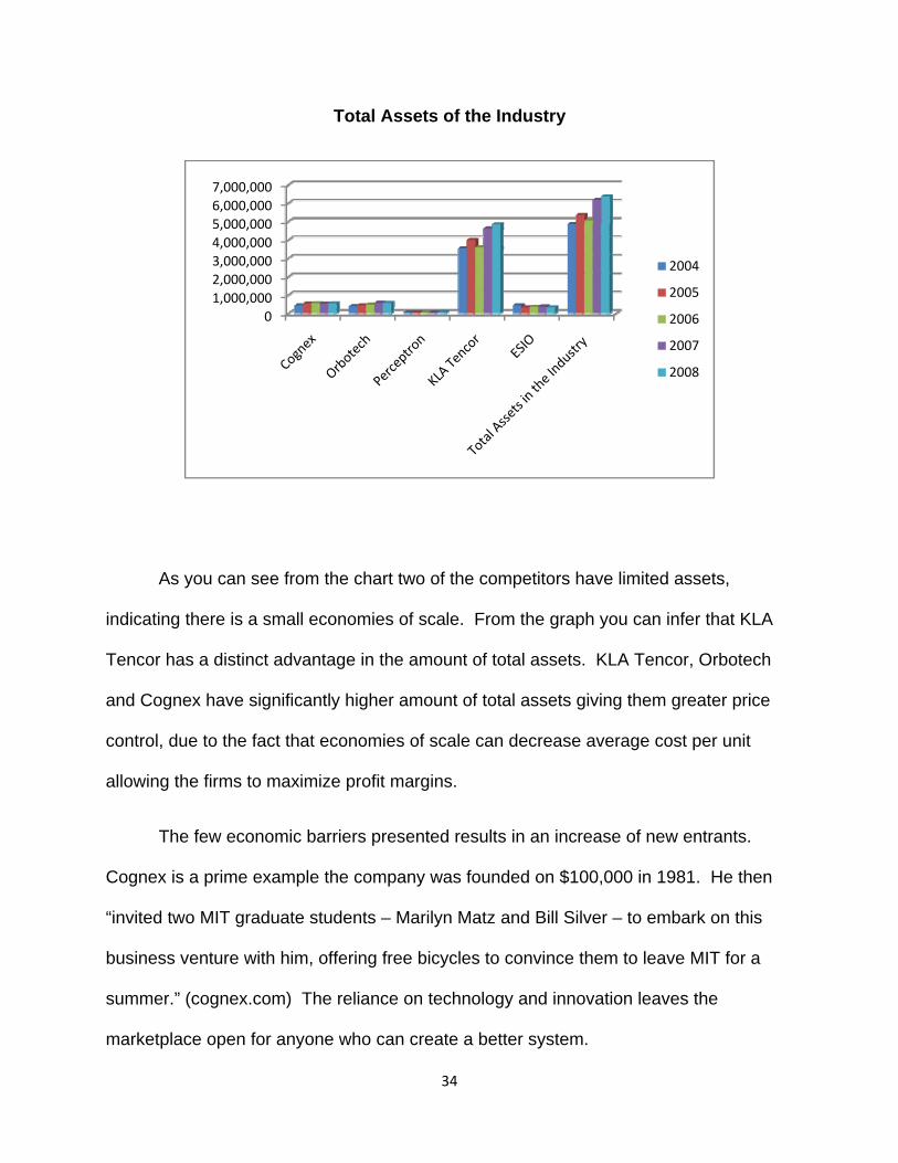
34
Total Assets of the Industry
As you can see from the chart two of the competitors have limited assets,
indicating there is a small economies of scale. From the graph you can infer that KLA
Tencor has a distinct advantage in the amount of total assets. KLA Tencor, Orbotech
and Cognex have significantly higher amount of total assets giving them greater price
control, due to the fact that economies of scale can decrease average cost per unit
allowing the firms to maximize profit margins.
The few economic barriers presented results in an increase of new entrants.
Cognex is a prime example the company was founded on $100,000 in 1981. He then
“invited two MIT graduate students – Marilyn Matz and Bill Silver – to embark on this
business venture with him, offering free bicycles to convince them to leave MIT for a
summer.” (cognex.com) The reliance on technology and innovation leaves the
marketplace open for anyone who can create a better system.
01,000,0002,000,0003,000,0004,000,0005,000,0006,000,0007,000,000
2004
2005
2006
2007
2008
35
Due to the ease of entering the industry firms are forced to decrease the cost of
products and enter a worldwide distribution system. The industry as a whole resulted to
globalizing their distribution strategically locating distribution system worldwide. Cognex
and Orbotech experience few barriers to achieve greater economies of scale, largely
due to the amount of outsourcing available. In conclusion we conclude that the
economies to scale are moderate, making it possible for new entrants to enter the
marketplace. However the fact that firms may enter does not indicate success.
First Mover Advantage
First entrants of an industry maintain a certain amount of advantage over new
entrants. New firms attempting to achieve market share may find themselves behind
established firms because “first movers might be able to set industry standards, or enter
into exclusive arrangements with suppliers of cheap raw materials”(Papelu & Healy).
In a technological dependent economy, first movers in the industry will possess
previously established contracts with suppliers and customers. All of the firms in the
industry have previously established contracts with suppliers of cheap raw materials.
Additionally the extremely high price of these products makes switching costs high,
therefore giving a firm a first mover advantage. This makes it extremely difficult for new
entrants to gain an advantage over previously established firms. This however does not
lower the threat of new entrants, due to the fact there are constant technological
advancements in the industry.
36
Distribution Access
Possible problems for new entrants into the industry can arise with channels of
distribution. There is “limited capacity in the existing distribution channels and high
costs of developing new channels” (Palepu & Healy). Currently globalized countries
can maintain a large competitive advantage and a large portion of the market share in
comparison to new entrants attempting to compete in a much smaller market share.
Cognex and their main competitors all currently operate globally. For example Cognex
is currently established in “52 countries worldwide,”(cognex.com) as well as KLA‐Tencor
maintains a significant presence throughout the United States, Europe and Asia. (KLA Tencor).
Orbotech also operates mainly out of Israel and the Middle East. This indicates that
previously established firms in this industry maintain a competitive advantage through
prior established distribution networks. This may limit new entrant’s ability to distribute
to existing markets, since these consumers currently are brand loyal.
Legal Barriers
In the electronic inspection and monitoring instruments market one very essential
aspect is to protect intellectual property rights. Firms are successful protecting this
information through trademarks and patents. Cognex currently attains “264 patents and
trademarks.” (10-k) One competitor Perceptron possess “27 patents” and
trademarks.(10-k) New entrants can find it extremely difficult to gain market share in
currently occupied markets, because of these stringent patent and trademark
requirements. In order for obtain superior product quality new entrants are often times
obligated to acquire products from a single source provider. The other option is to
37
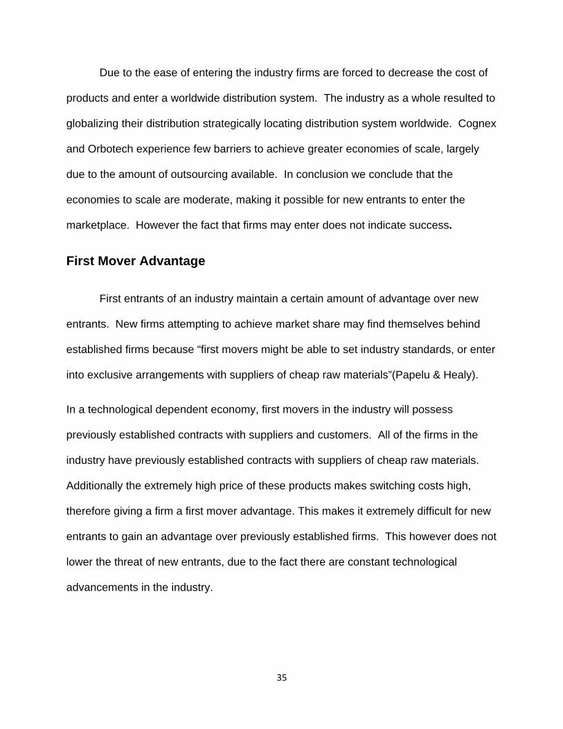
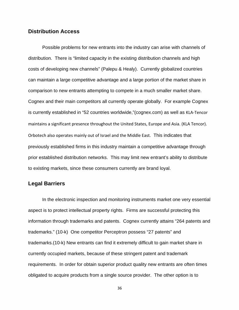
allocate significant amounts of capital to research and development allowing the
company to bypass existing suppliers and technology. The following chart displays the
amount of capital distributed to research and development.
From the chart you can visualize it is imperative for the firms in the industry to
invest heavily in research and development to avoid breaching copyright and trademark
infringements of other firms. Otherwise they are forced to expend extra funds to
purchase existing products from well established firms in the industry.
Conclusion
There are low economies of scale, meaning firms entering the market may do so
with little investment. Although it may be fairly easy to enter, existing firms may have an
advantage as their contracts and relations with suppliers is already established. The
0
0.1
0.2
0.3
0.4
0.5
0.6
KLA Tencor Perceptron Orbotech Cognex ESIO
2004
2005
2006
2007
2008
38
cost of developing new distribution channels also poses a problem for firms entering the
market. Several legal barriers have also made it difficult for new firms to establish
themselves. Every firm in the industry uses patents, trademarks and long term contracts
to protect themselves from firms attempting to increase their market share.
The scientific and technical instruments market is a very accessible market to
enter with low capital. But however legal barriers and the emphasis and new
technological advances can make it difficult for new entrants to be successful. Currently
established distribution markets and brand loyalty give long-standing firms a competitive
advantage. Contracts, copyrights, and trademarks can also allow initial firms a first
mover advantage.
Threat of Substitute Products
In the scientific and technical instruments market, there are various motivations
to substitute a product for a different one. One of the factors affecting substitution is
price. Price is very relative in the relation of substitutes because products in the
industry are very expensive they are not everyday goods. Performance additionally
plays a large role in the substitution process. The most important element of this
industry is the ability to ensure perfection among produced products.
Due to the mass quantity of firms that would desire a electronic inspection and
monitoring of this nature many have been produced to attempt to mimic the task,
allowing for a variety of products in the market. As technology advances devices for
39
manufacturing monitoring can become more universal and less specialized. Less
specialized products have a higher threat of substitute products.
Performance is absolutely vital to ensure success in the market. In the industry
there is an elevated demand for smaller, faster, and more efficient products allowing
several substitutes to be created. This constantly evolving industry allows a vast
amount of consumers to play an active role in the market. Consequently, firms in the
industry must be able to emphasize both on price and performance. Although some will
sacrifice performance in order to cut price most consumers are not. However a superior
performance and superior price can force consumers to acquire a more affordable
product.
Costumers Willingness to Switch
In an industry dominated by technological innovation, differentiation, and
constant improvements substitute products are viable in the industry. Firms are
constantly endowing capital in order to create new advancements. Most products and
technology are protected by legal copyrights, and patents. Reverse engineering allows
for similar products to be produced quickly. The industry is an active market that allows
consumers to find the most effective product at an agreed upon price.
40
Conclusion
Price is fairly consistent throughout the industry, as most firms are willing to pay
a high price for a premium product. The products in this industry are highly specialized
and differentiated leading to a low customer willingness to switch. Additionally halting
customers to switch is the long life of the product, every company in the industry offers
various types of warranty programs additionally to keep the product operating properly
and at full satisfaction of the consumer.
Bargaining Power of Customers
To determine the actual bargaining power of a firm’s customer base, analysts
begin by examining the core markets the firm operates in and to whom they sell their
products. The scientific and technical instruments market operates in three specific
markets: semiconductor and electronic capital equipment, surface inspection, and
discrete factory automation. The original equipment manufacturers (OEM) who produce
semiconductor and electronic capital equipment are major customers in this market.
Other industries these products are present are in the automotive, consumer products,
electronics, food and beverage, medical devices, pharmaceutical, packaging, solar, and
glass. The discrete automation manufacturing market supplies manufacturers of several
industries. They include: automotive, consumer electronics, food, beverage, health care,
pharmaceutical and aerospace industries. The customers of the surface inspection
market include firms that manufacture metals, paper, non-wovens, plastics, and glass.
41
Firms in these industries purchase this equipment from authorized third party dealers or
a direct sales force. Due to the wide variety of the product specifications and growing
customer needs, it is important that firms maintain strong customer relations.
Price Sensitivity - Customer
Just as external relationships are crucial, it is also important to examine price
sensitivity in order to establish a fair market price. “The importance of the product to the
buyers’ own product quality also determines whether or not price becomes the most
important determinant of the buying decision”(Palepu & Healy). Customers in this
industry rely strongly on their brand image; therefore many are willing to pay a premium
on capital equipment to ensure the quality of their products. Patents are often used to
protect intellectual property used in developing products in this industry. For example,
Cognex has approximately 264 patents while their competitor Perceptron, accounts for
27. Due to the high specification of the products in the industry customers have low
price sensitivity.
Relative Bargaining Power - Customer
The relative bargaining power with respect to customers is “the cost to each party
of not doing business with the other party” (Palepu & Healy). In other words, the more
firms and alternative products that the customers have to choose from the more
customers have bargaining power over suppliers. In this case, the customer base within
42
the industry has a demand for highly specialized products that meet their needs. Firms
in this industry have bargaining power over their customers because these products are
essential to their business and there business operating effectively. However, the loss
of any customer or potential orders could adversely affect business operations. Every
firm in the industry has its large customer base and additionally a small customer base.
These larger customer bases in general account for a much large percentage of sales
than do the smaller customers. Due to the nature of this industry, relative bargaining
power over customers is considered to be moderate.
Customer Switching Cost
Switching cost refers to how easily customers can switch from one product to
another. Although this is a concern in some industries where products are easily
substituted, this industry proves otherwise. The fact that firms in the industry rely on
differentiation, switching costs are particularly high. The firms in this industry produce
technology that many customers find essential for their business, limiting their ability to
seek alternative products. Additionally the price of the products being considered a
exclusive good make it difficult to switch from product to product, without a significant
loss of capital Therefore, customer switching cost in this industry are high.
43
Conclusion
The scientific and technical instruments industry is a highly differentiated market,
resulting in a very low quantity of substitutable products. Additionally the high price of
the products also makes it very hard to switch, without losing large amounts of
investment.
Bargaining Power of Suppliers
Several of the concepts used to determine the ultimate power of customers are
also incorporated when analyzing the sensitivity of price between firms and their
suppliers. Depending on the size, number and proximity of suppliers, prices can
fluctuate to a great extent. If not controlled adequately, high prices from suppliers can
result in large operation costs. In industries where many suppliers operate, bargaining
power of the purchasing firm is high. In contrast, in an industry with one or few
suppliers there is little to none bargaining power. Cognex and orbotech conclude that
they are firms that obtain components from single source suppliers (Cognex and
Orbtech 10-ks). KLA Tencor, ESIO, and Perceptron also have contracts with suppliers
make the products exclusively available to the individual firm. Due to the lack of
alternative suppliers, these single source suppliers can simply set a price that firms
must consent to.
44
Price Sensitivity – Supplier
As mentioned previously, the number of suppliers can greatly influence the cost
of operations for a business. In an industry that is greatly dependent on differentiation,
the number of suppliers is already limited to firms. Cognex, KLA Tencor, Orbotech,
Perceptron, and ESIO furthermore have a single supplier contracts, prohibiting some
suppliers from supplying any other firms. This can greatly limit firm’s ability to find an
alternative low cost provider.
Relative Bargaining Power – Supplier
In a differentiated market where there are a limited number of supplying firms,
the bargaining power is generally fixed. As a result, firms tend to enter into long term
contracts with their suppliers in order to keep costs relatively stable, and because they
simply have no other means of acquiring equipment. These long term contracts,
coupled with a small number of suppliers makes it difficult for firms to find alternative
low cost options. Therefore, suppliers in this industry have low relative bargaining power
over firms.
Conclusion
Suppliers in the industry are limited due to the contracts and differentiated products.
Additionally the high switching costs lowers the amount of power they maintain over
buyers. These conditions make it very difficult for the firms in the industry to look
45
around for other alternatives. The industry is not affected to market fluctuations, as well
as inflation because of the long term contracts they enter with the firms.
Industry analysis
Superior product quality:
Firms can compete on a product that; lowers the cost of inspection and detection,
produces accuracy and serves their industry closer than the competitors. Vision devices
in highly automated production lines need to be able to provide guidance, identification,
and inspection at a high speed and register moving elements accurately and reliably.
Accurate and reliable detection can ensure that the original product manufacture has a
finished good that is on par with their quality standards. Deviations of quality in
production can cause unnecessary loss of productivity and other costs to
manufacturers. KLA Tencor offers superior products quality by guaranteeing
“extensive refurbishment, testing, and certification minimize investment risks,
while increasing equipment value. As well as Cognex, Orbotech, Perceptron, and
ESIO that all offer extensive warranty and guarantees to ensure superior product
quality. Some firms have been able to lower costs of inspection with specific products.
Technological advances have allowed some vision systems to become more general, in
that they don’t require as much specialization to perform a wide array of operations.
46
Superior product variety:
Visual systems allow firms to detect orientation, identify, to inspection, or
measure dimensions. Not all firms in any market are the same or use the same
production process. The larger deviation between firms is the products that they
produce. In order to be successful in the vision inspection market you must be able to
inspect and ensure perfection on a variety of products that are a variety of sizes,
shapes, materials, and even color. The visual identification tools available can pinpoint
the exact location and orientation of a variety of products. For example id scanners can
be used in warehouses, supermarkets, food and beverage industries and consumer
packaging. KLA Tencor who specializes in wafer identification, while Cognex and
Orbotech use a system called surface inspection systems. Defects do come in all
shapes and sizes. Some markets may have a defect in the printing department; others
may have one in a manufacturing department. Ideally you would need to be able to
inspect every department in the manufacturing process from beginning to end. While at
the same time they must be able to inspect and guarantee perfection in a wide variety of
products. These products can serve a multiple amounts of industries such as wood,
metals, papers, nonwovens, plastics and glass, automotive, consumer products,
electronics, food and beverage, medical devices, pharmaceutical, packaging and solar.
Available technology can even assist with products in automation and determine the
dimensions of a product that does not possess a defined shape. By allowing firms to
inspect every aspect of their product, you allow those firms to guarantee perfection back
47
to their customers, heavily increasing their market share. As well as presenting this
firms with a more marketable product. Electronic inspection devices do not come in only
one shape or size. There is a wide variety of products offered to enable any
manufacture to incorporate them into a current line with little disturbance in current
production.
Superior customer service:
Due to evolving nature of automated assembly lines customer service is a necessity
among firms. Automated lines depend on essentially all products running smoothly so if
detection devices or software are on the failing, production capabilities can be
hampered. Companies in this industry provide training for their clients on several
different technological levels from beginner to advance. This advanced training can add
considerable amounts of value to a firm. Additionally this training can prevent a wide
variety of problems from occurring after the product is installed, and when these
problems do occur the provided training can aid in ensuring a rapid repair. This will
reduce the amount of revenue lost by manufacturing lines being halted. This
educational material is more often than not free of charge to customers. Firms will send
out a magnitude of informational software and literature along with several trainers
permit a hands on approach. Around the clock customer service call centers are
available from Cognex, KLA Tencor, Orbotech, Perceptron, and ESIO. Operated by
highly trained and intelligent individuals guaranteeing your product will be operational
48
twenty four hours a day. These first-class customer service plans can improve client’s
perception of the industry and the market, and will refrain customers from substituting
your product for another due to small predicaments with the product. The large
customer based served by the industry includes the food industry, electronics, printing,
textiles, glass, packaging and many others. These industries cannot afford to have
production lines shut down for extended periods of time and therefore rely on these
products to be successful.
Research and Development
In order for firms to keep pace with the industry’s accelerating learning curve,
they must spend substantial amounts of capital on R&D. Kla-Tencor stated in their
annual report “that continued and timely development of new products and
enhancements to existing products are necessary to maintain a competitive position”
(KLA-TENCOR 10-K). Therefore, firms in this industry must invest a percentage of
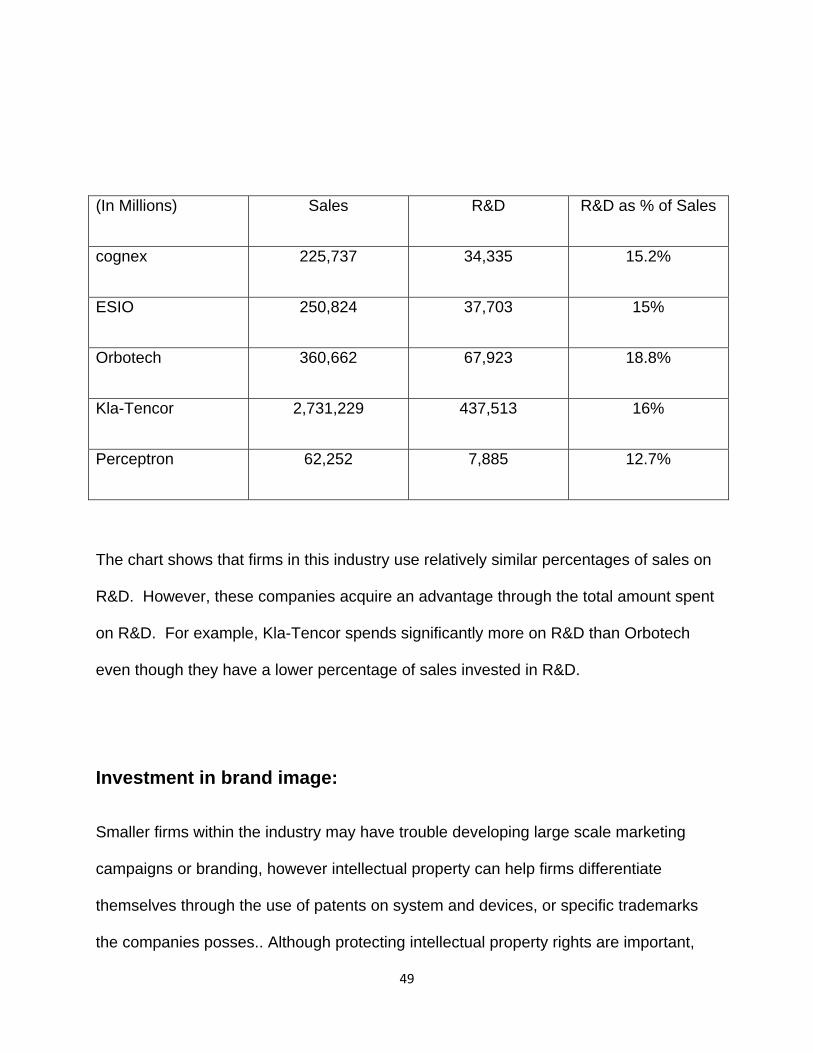
sales in research and development to remain effective. The chart below provides
information about net sales and R&D of rival firms in this industry.
49
The chart shows that firms in this industry use relatively similar percentages of sales on
R&D. However, these companies acquire an advantage through the total amount spent
on R&D. For example, Kla-Tencor spends significantly more on R&D than Orbotech
even though they have a lower percentage of sales invested in R&D.
Investment in brand image:
Smaller firms within the industry may have trouble developing large scale marketing
campaigns or branding, however intellectual property can help firms differentiate
themselves through the use of patents on system and devices, or specific trademarks
the companies posses.. Although protecting intellectual property rights are important,
(In Millions) Sales R&D R&D as % of Sales
cognex 225,737 34,335 15.2%
ESIO 250,824 37,703 15%
Orbotech 360,662 67,923 18.8%
Kla-Tencor 2,731,229 437,513 16%
Perceptron 62,252 7,885 12.7%
50
their functionally is to protect “technological expertise and develop new and better
technologies”(kla-Tencor). Additionally firms invest in advertising to get the frims name
more familiar with the public. KLA Tencor invests on average 4.58 million dollars a year
in advertising while Cognex invests 1.74 million a year in advertising. However firms
hoping to build off of their core competencies need to have products that end-users can
associate with, especially if companies serve the market.
Value Creation analysis
Superior customer service
With new products evolving daily in the scientific and technical industry there
remains a lot of room for inexperience on the job. Manufactures that integrate new
systems, however do not offer employees adequate training and education in the field
will not be successful. Without proper training employees will run into an ample
amount of technical problems resulting in delays in production and manufacturing lines.
They also will not be able to guarantee precision and flawless work, which will greatly
damage their products image, and not to mention market share and profits Behind all
of these vision professionals lies a wealth of support resources, including live, online,
and video-based training; online conferencing; software downloads; our searchable web
knowledge base; and worldwide technical support . Firms such as Intel and Applied
Materials are spending less on capital equipment due to the current economic situation.
51
It is more important than ever for customers to maintain relationships with their
suppliers. (WSJ)
Workshops and Seminars
Before purchasing a product, there is a large array of workshops available in
order to acquire prior information about the product to make sure it will be the right
purchase. These workshops are available worldwide and open to the public. There
are additionally seminars available on the internet to provide easily accessible
information to any consumer worldwide. These seminars are available for all of the
leading technological progress available to purchase.
Installation
With the purchase of a Cognex system, you are provided with a world class
installation team to apply the products to your current manufacturing process “they
adapt automatically and never need adjustment”. (Cognex.com) This installation is not
only quick and effective customers are not forced to change a manufacturing process in
order to fulfill to criteria to make the product effective. This amounts to little or no delays
in manufacturing process. With the professional installation Cognex offers a wide
variety of training programs for customers.
Training
52
The mass amounts of training programs offered, greatly increase companies
chances of succeeding. After installation a highly trained and experienced employee
will come educate, and prepare you for your product. You will be instructed with
directions on use of the product, but also with information on how to repair any
malfunctions. As well as a wide variety on in class training programs that can be
attended, that “most are free-of-charge* and we provide many different vehicles to help
you learn more about how to improve your process through machine vision
inspections..” (Cognex.com) These classes will provide not only educational
information about the product, but also provides a hands on approach to allow students
to master the product. Training programs are also provided on the web, if you are not
able to make it to a class room session, giving full accessibility to knowledge of the
product. This allows manufacturers to cross train employees, providing producers with
a much more efficient manufacturing process.
Online Meeting Rooms
In Cognex’s online meeting rooms you are able to communicate with other
customers around the world allowing customers to entertain others with questions they
might have previously had, or to give each other advice about new equipment. There
are two online meeting rooms available to anyone with the internet anywhere in the
world. These rooms have a capacity to accommodate anyone, allowing all customers
the same amenities.
Smartlist
53
This program allows customers to email each other with questions. Smartlist will
allow you to see other customers sharing the same products and services you are
currently enjoying as well as other products you may be interested in the future.
24 Hour Customer Service
Customer service representatives are available twenty four hours a day, three
hundred and sixty five days a year. All customer service representatives are trained
with knowledge of all current programs and products offered in the line. These
representatives can be contacted through a variety of ways including over the phone,
email, and via online chat. These services stations are located worldwide in able to
prevent a language barrier of any kind. As opposed to Orbotech whom only provides
five worldwide centers. (Orbotech.com)
In an industry that is continually increasing the amount of knowledge it takes to
be successful, everyone will need a helping hand. At Cognex “Customers are our
number one priority, and listening to them is always the first step. Cognex sales
engineers and application specialists are located around the world, to provide
assistance wherever and whenever needed.” (Cognex.com) The wide array of
customer service and training available anyone can become a knowledgeable Cognex
customer.
54
Superior Product Variety
In the scientific and technical industry all competitors are endlessly competing on
product size and quality. Cognex strives to make their product smaller and more widely
available for all areas of the product line, and for numerous markets. Currently Cognex
services the “automotive, the medical, the solar, the semiconductor and electronic, the
pharmaceuticals, the paper, plastics, nonwovens web inspection, the food and
beverage, packaging, the metal and glass surface inspection, and general
manufacturing markets” (Cognex.com). These markets all require different products in
order for them to be successful, currently Cognex reinvested $34,335,000 into research
and development in order to meet this needs of its customers. With more advanced
products being introduced to current customers, it is also very available to other markets
similar in nature. By offering more advanced products and numerically a greater
number Cognex can greatly improve its market share. Cognex presently is the number
“one in the widest product range, providing robust and cost effective solutions to every
application.” (Cognex.com) By producing a wide variety of products Cognex is able to
offer numerous products at different prices to accommodate any and all consumers.
Research and Development
In the scientific and technical instruments industry it is vital to respond to new
technological transformations within the industry. Cognex states that “the failure to
develop new products could result in a loss of market share and decrease revenues and
profits” (Cognex 10-k). Cognex has increased the amount of revenue used for R&D
55
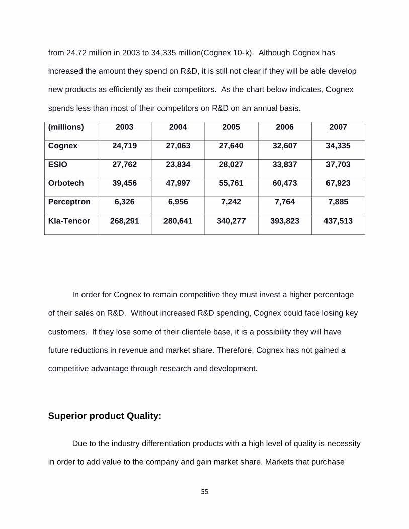
from 24.72 million in 2003 to 34,335 million(Cognex 10-k). Although Cognex has
increased the amount they spend on R&D, it is still not clear if they will be able develop
new products as efficiently as their competitors. As the chart below indicates, Cognex
spends less than most of their competitors on R&D on an annual basis.
(millions) 2003 2004 2005 2006 2007
Cognex 24,719 27,063 27,640 32,607 34,335
ESIO 27,762 23,834 28,027 33,837 37,703
Orbotech 39,456 47,997 55,761 60,473 67,923
Perceptron 6,326 6,956 7,242 7,764 7,885
Kla-Tencor 268,291 280,641 340,277 393,823 437,513
In order for Cognex to remain competitive they must invest a higher percentage
of their sales on R&D. Without increased R&D spending, Cognex could face losing key
customers. If they lose some of their clientele base, it is a possibility they will have
future reductions in revenue and market share. Therefore, Cognex has not gained a
competitive advantage through research and development.
Superior product Quality:
Due to the industry differentiation products with a high level of quality is necessity
in order to add value to the company and gain market share. Markets that purchase
56
Cognex vision systems require that products satisfy their manufacturing process needs
in order for them to be able to realize their own products. Products that provide a
greater degree of accuracy, especially for the electronics industry, are more sought after
because they insure that the manufacturing process is running according to plan without
expensive delays in production. Congenx provides for this necessity by providing
products that cater to a need of accurate and reliable measurements and inspections.
Identification and inspection systems for industries such as the electronics industry
require high-speed and accurate detection of defects in minute components “Cognex’s
In-Sight® 1720 series wafer ID reader quickly and reliably reads codes”(Cognex 10-k),
although this may seem as industry standard Cognex has devoted much of their time
and effort into developing better products for the electronics markets, “In 2000 sales to
semiconductor and electronics capital equipment manufactures represented
approximately 61% of the companies’ total revenue”(Cognex 10-k). Cognex has been
leading machine vision technologies and is able to capture sales from companies who
need specific solutions. Cognexs’ innovative tool PatMax®, enabled companies to
detect defects in hard to identify surfaces such as reflective solar panels with better
accuracy (Cognex.com).Tools such PatMax® as can lower the cost of inspection by
reducing expensive returns and new materials. Further development of In-Sight®
product lines and other lines has helped Cognex develop industry specific solutions that
maximize accuracy. Further devotion to accuracy and vision technologies in their
products can lead Cognex to further increase their market share and help gain a
competitive advantage over firms competing in similar markets. Cognex also has the
capacity to produce generalized goods that can sevrve a basic amount of functions
57
Conclusion
To create value within a firm customer service, superior product quality, research
and development, and product variety are all necessities. Cognex has a market full of
competitors. This means that the product lines must be flexible enough to serve any
industry. The variety of products firms offer can determine whether or not they are
flexible enough to become a major force in the industry. Product quality is very
important as consumer firms have a zero tolerance on defective products. The training,
online meeting rooms and 24 hour customer service are some intangibles that create
value for Cognex.
Formal Accounting Analysis
Introduction
The accounting procedure is a very important operation in business. It reports
how a firm accounts for its transactions, and in turn, helps to establish a value for the
firm. Due to the fact, that most of the numbers are either exposed to some degree of
manipulation or error there is need for a method to standardize this distortion.
Consequently it is required for companies to follow the Generally Accepted Accounting
Principles.
However even thought this practice was created and is enforced by the United
States Government under the Sarbanes Oxaley Act, there is still room for error. This
allows firms to still manipulate numbers in whatever they deem necessary. One
practice of manipulation is by deflating or inflating net income. By inflating net income
58
firms are able mislead investors by presenting a more profitable firm. Additionally by
deflating net income a firm is able to reduce tax expenses or deceive competitors.
These practices are legal under the GAAP principles, and therefore elevate the
importance for a system to recognize these instances.
In order to locate the manipulation an accounting analysis is used using six
steps. These steps evaluate a firm’s accounting quality. Step one is to identify principal
accounting policies. This involves identifying key success factors and potential risks in
an industry. Step two is to assess accounting flexibility. The flexibility of the accounting
policies can have a significant impact on the reported financial performance of a firm
(Palepu & Healy). Step three is to evaluate accounting strategy. After the flexibility of
the policies are examined, it is necessary to assess accuracy and bias within the
reporting. Step four evaluates the quality of disclosure. GAAP establishes minimum
criteria for disclosure, but company managers have final discretion when reporting
financial statements. Step five is to identify potential red flags within the financial
statements. These are indicators that analysts should examine to assess the accuracy
of the reports. The final step is to undo any accounting distortions. If any numbers
appear to be inaccurate, analysts should restate the reports in order to reduce distortion
as much as possible (Palepu & Healy).
Key Accounting Policies
Cognex key success factors include product differentiation, superior quality,
global distribution and value creation for the customer. The prior factors are a firms
type one Key Accounting Policies that allow you to analyze the key success factors in
59
relation to disclosure. These success factors are driven by the accounting of day to day
business operations. Different accounting policies create different images of firms,
depending how management decides to report the financials. This creates the
opportunity for management to distort financial statements in order to hide potentially
negative information or create a false image.
Secondly the type two policies that refers to distortion. These distortions can
occur in areas regarding research and development, goodwill, defined pension plans,
foreign currency risk, and operating and capital leases. GAAP allows managers to use
the most appropriate accounting techniques because of managements’ “superior
knowledge of the business to determine how best to report the economies of key
business events” (Palepu & Healy). It is important to analyze each area where there is a
potential for distortion in order to create a true and accurate picture of the firm and its
industry.
Goodwill
A major operation of many firms is acquiring subsidiaries and smaller companies
to increase market share and implement new technology. When a new firm is acquired,
it is assigned a price at market value. However, many companies purchase subsidiaries
for an amount in excess of their fair market value. This additional amount paid above
market value is referred to as goodwill. Goodwill is located on the balance sheet as an
intangible asset. It refers to the extra “value” obtained by the structure of a business’s
operations. Cognex has two units to which it reports goodwill, the Modular Vision
System Division (MVSD) and the Surface Inspection Systems Division (SISD).
Currently, the MSVD reports a goodwill value of $83,328,000 and the SISD reports
60
goodwill at $3,133,000. This is a very large number for Cognex in relation to the ten
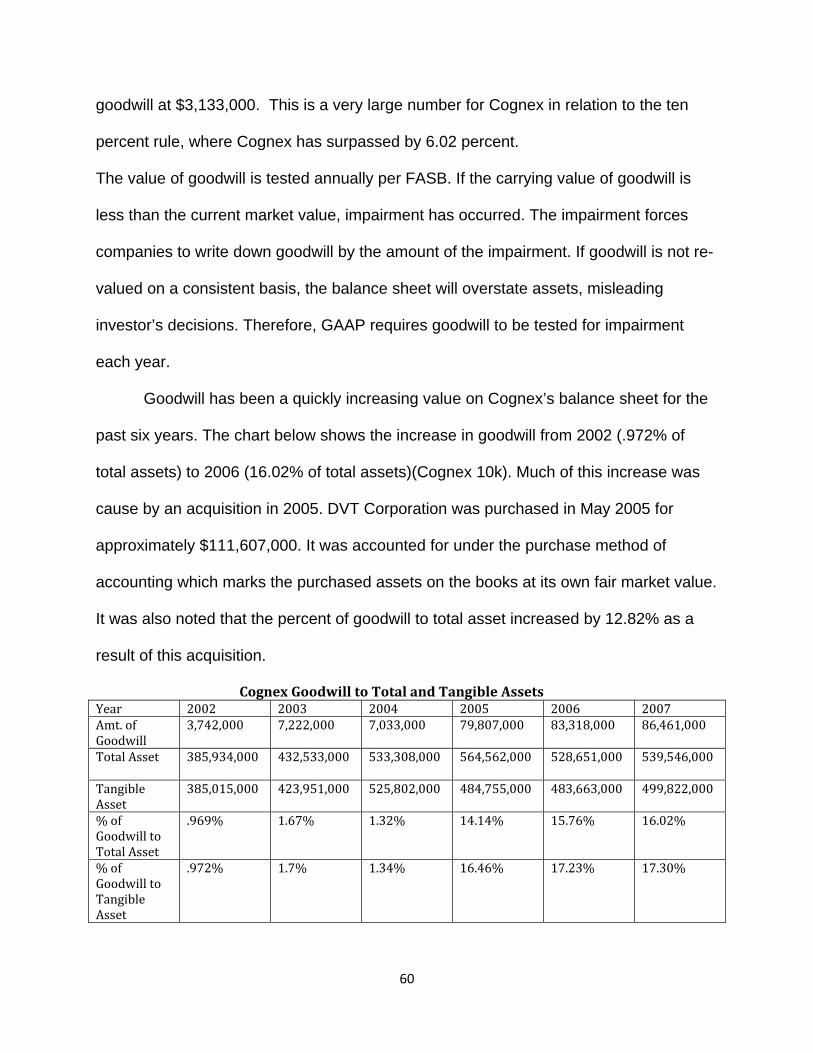
percent rule, where Cognex has surpassed by 6.02 percent.
The value of goodwill is tested annually per FASB. If the carrying value of goodwill is
less than the current market value, impairment has occurred. The impairment forces
companies to write down goodwill by the amount of the impairment. If goodwill is not re-
valued on a consistent basis, the balance sheet will overstate assets, misleading
investor’s decisions. Therefore, GAAP requires goodwill to be tested for impairment
each year.
Goodwill has been a quickly increasing value on Cognex’s balance sheet for the
past six years. The chart below shows the increase in goodwill from 2002 (.972% of
total assets) to 2006 (16.02% of total assets)(Cognex 10k). Much of this increase was
cause by an acquisition in 2005. DVT Corporation was purchased in May 2005 for
approximately $111,607,000. It was accounted for under the purchase method of
accounting which marks the purchased assets on the books at its own fair market value.
It was also noted that the percent of goodwill to total asset increased by 12.82% as a
result of this acquisition.
Cognex Goodwill to Total and Tangible Assets Year 2002 2003 2004 2005 2006 2007Amt. of Goodwill
3,742,000 7,222,000 7,033,000 79,807,000 83,318,000 86,461,000
Total Asset
385,934,000 432,533,000 533,308,000 564,562,000 528,651,000 539,546,000
Tangible Asset
385,015,000 423,951,000 525,802,000 484,755,000 483,663,000 499,822,000
% of Goodwill to Total Asset
.969% 1.67% 1.32% 14.14% 15.76% 16.02%
% of Goodwill to Tangible Asset
.972% 1.7% 1.34% 16.46% 17.23% 17.30%
61
This large increase in goodwill is supported in part by the additional value
created by the DVT acquisition. “With the acquisition of DVT Corporation, we
immediately gained a worldwide network of distributors, fully trained in selling and
supporting machine vision products.” (Cognex 10 K)As this acquisition surely added
value to Cognex, the unusually large increase in goodwill is a red flag indicator, as
assets may be overstated. An impairment test is needed to re-value goodwill and
present assets in an accurate manner. KLA-Tencore has seen similar changes on its
balance sheet in recent periods as well. In 2006 and 2007 the company made several
acquisitions to expand product lines. The acquisitions brought about an increase of
$264,956,000 in aggregate goodwill to the asset account.
Not all companies in the industry use goodwill quite the same. Several of
Cognex’s competitors have a very small amount of goodwill, if any at all. Orbotech
currently operates with $12,466,000 as goodwill. ESIO only reports $1,442,000, and
Perceptron carries zero goodwill on its books.
Research and Development
Companies expend large amounts of cash and valuable assets on research and
development. It is imperative that firms consistently work to expand product lines and
market share. Developing new manufacturing methods to speed up production and
entering new market niches with additional products are two ways managers try to beat
the competition. However, much of the money allocated to research and development is
expensed on failed projects and never seen again. Just as allocating money to R&D
involves risk, there is also the possibility of reward. A successful R&D project can create
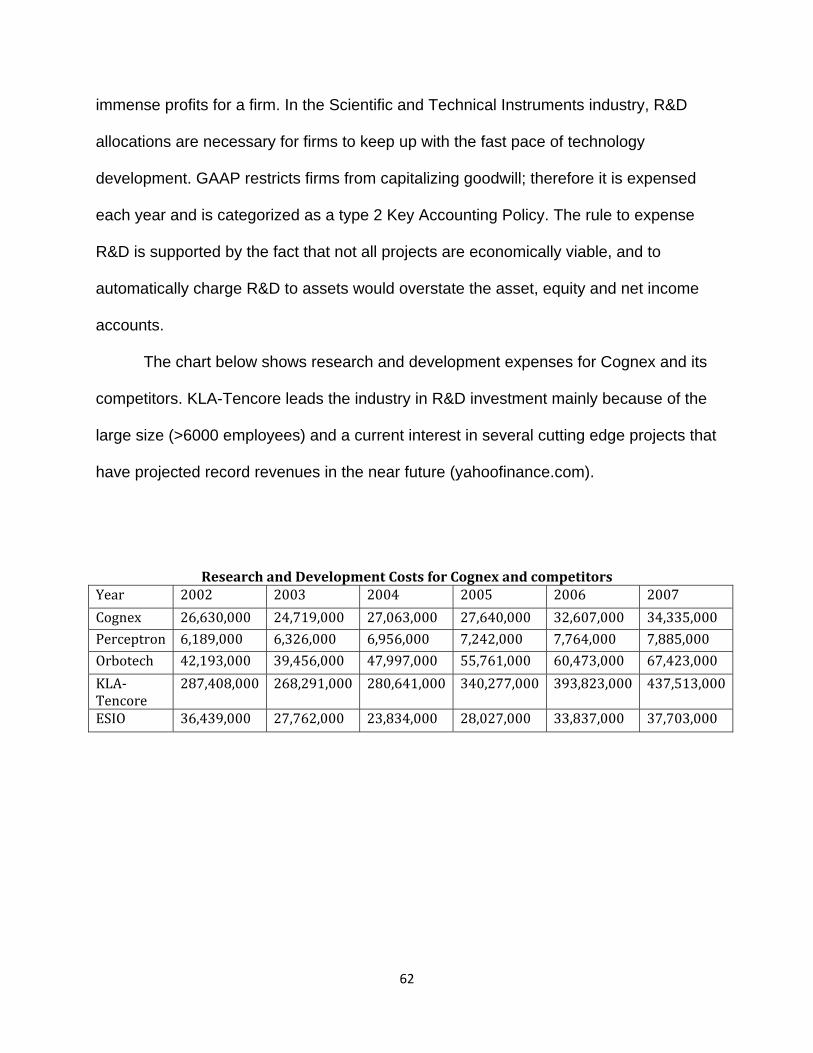
62
immense profits for a firm. In the Scientific and Technical Instruments industry, R&D
allocations are necessary for firms to keep up with the fast pace of technology
development. GAAP restricts firms from capitalizing goodwill; therefore it is expensed
each year and is categorized as a type 2 Key Accounting Policy. The rule to expense
R&D is supported by the fact that not all projects are economically viable, and to
automatically charge R&D to assets would overstate the asset, equity and net income
accounts.
The chart below shows research and development expenses for Cognex and its
competitors. KLA-Tencore leads the industry in R&D investment mainly because of the
large size (>6000 employees) and a current interest in several cutting edge projects that
have projected record revenues in the near future (yahoofinance.com).
Research and Development Costs for Cognex and competitors Year 2002 2003 2004 2005 2006 2007Cognex 26,630,000 24,719,000 27,063,000 27,640,000 32,607,000 34,335,000Perceptron 6,189,000 6,326,000 6,956,000 7,242,000 7,764,000 7,885,000Orbotech 42,193,000 39,456,000 47,997,000 55,761,000 60,473,000 67,423,000KLA‐Tencore
287,408,000 268,291,000 280,641,000 340,277,000 393,823,000 437,513,000
ESIO 36,439,000 27,762,000 23,834,000 28,027,000 33,837,000 37,703,000
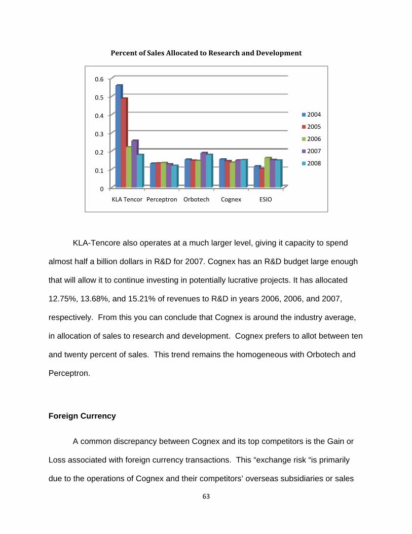
63
Percent of Sales Allocated to Research and Development
KLA-Tencore also operates at a much larger level, giving it capacity to spend
almost half a billion dollars in R&D for 2007. Cognex has an R&D budget large enough
that will allow it to continue investing in potentially lucrative projects. It has allocated
12.75%, 13.68%, and 15.21% of revenues to R&D in years 2006, 2006, and 2007,
respectively. From this you can conclude that Cognex is around the industry average,
in allocation of sales to research and development. Cognex prefers to allot between ten
and twenty percent of sales. This trend remains the homogeneous with Orbotech and
Perceptron.
Foreign Currency
A common discrepancy between Cognex and its top competitors is the Gain or
Loss associated with foreign currency transactions. This “exchange risk “is primarily
due to the operations of Cognex and their competitors’ overseas subsidiaries or sales
0
0.1
0.2
0.3
0.4
0.5
0.6
KLA Tencor Perceptron Orbotech Cognex ESIO
2004
2005
2006
2007
2008
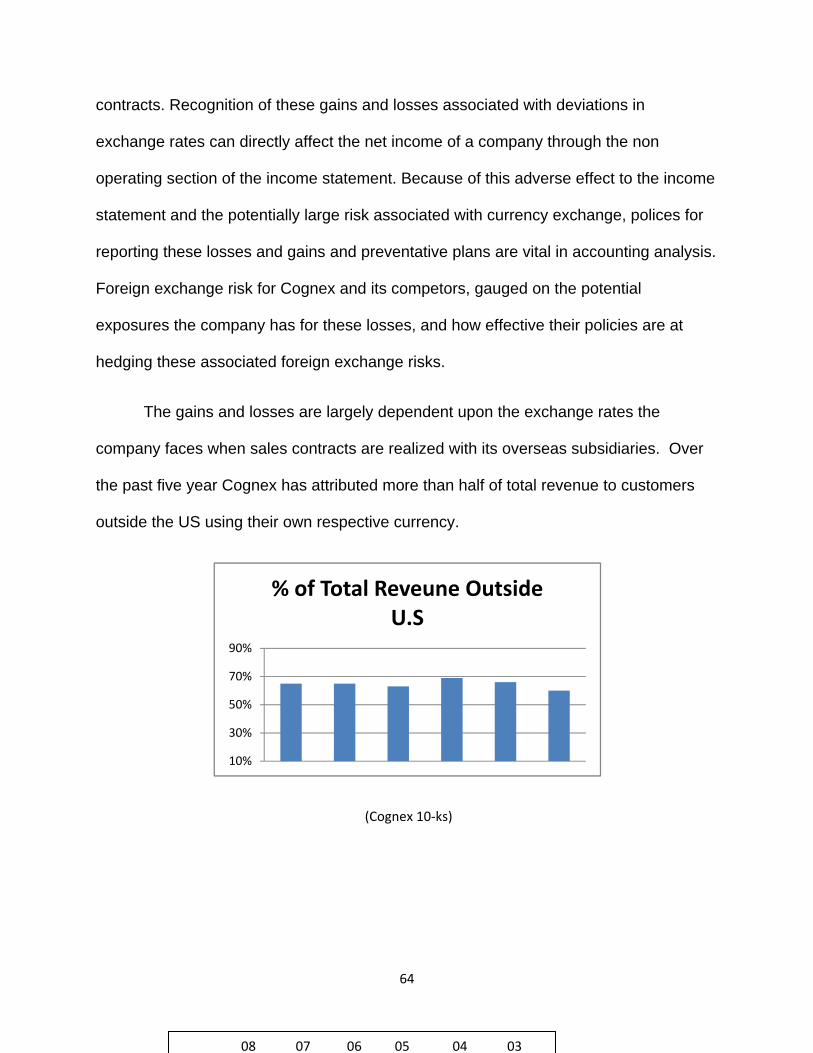
64
contracts. Recognition of these gains and losses associated with deviations in
exchange rates can directly affect the net income of a company through the non
operating section of the income statement. Because of this adverse effect to the income
statement and the potentially large risk associated with currency exchange, polices for
reporting these losses and gains and preventative plans are vital in accounting analysis.
Foreign exchange risk for Cognex and its competors, gauged on the potential
exposures the company has for these losses, and how effective their policies are at
hedging these associated foreign exchange risks.
The gains and losses are largely dependent upon the exchange rates the
company faces when sales contracts are realized with its overseas subsidiaries. Over
the past five year Cognex has attributed more than half of total revenue to customers
outside the US using their own respective currency.
(Cognex 10‐ks)
10%
30%
50%
70%
90%
% of Total Reveune Outside U.S
08 07 06 05 04 03
65
Sales to customers outside the US hasn’t experienced much deviation, however,
with more than half of sales made in currencies other that the U.S. Dollar, revenue
recognition in one period may differ significantly when the accounts are collected in
another due to currency fluctuations. Cognex is not alone in their dispersion of revenue
in the form of other currency; companies within the industry face similar revenue
distributions to overseas buyers and expose themselves to potential risk.
An important accounting practice that “hedges” these contracts so that the
company will be able to realize actual amounts in US dollars and avoid losses of
currency fluctuation involves the use of forward contracts. Cognex uses forward
contracts to thwart currency fluctuations effects on the balance sheet. These contracts
according to Cognex will help accounts receivable be realized closer to their actual
amount for the year, however their effectiveness depends on expected exchange rates
and receivable forecasts. Both Cognex and its competitors use these forward contacts
to prevent their accounts receivable from being under realized when collected.
Companies will use these forward contracts when deemed necessary, other accounting
treatments such as future contacts and currency swapping have a similar effect to
hedge against currency fluctuations although Cognex’s main derivative instatement are
forward contracts.
In order to effectively hedge against foreign currency exposure “the company
evaluates its foreign currency exposures on an ongoing basis and makes adjustments
to its foreign currency risk management program as circumstances change.” (Cognex
10-k). Disclosure of foreign currency risk polices in the notes to the financial statement
is essential to value the total revenues of a company or analyze the assets and liabilities
66
of the companies forging subsidiaries. Proper management discussion and analysis of
foreign currency risk management policies is equally important to understand the logic
of recording gains or losses in the value of overseas subsidiaries assets and liabilities or
“Balance sheet Exposure”(Orbotech 10-k)
Foreign Exchange risk is Exchange rate fluctuations can have an adverse effect
on both the balance sheet and the income statement so companies such as Cognex
that display increasing amounts of potential risk should have effective currency risk
management programs. Effective currency risk management programs are necessary to
hedge operating transactions and balance sheet amounts to their actual values.
Successful Preventative accounting policies are a necessity to hedge against these
fluctuations in currency exchange rates.
Assessing Accounting Flexibility
Introduction
When accounting for business operations, different policies and regulations determine how the
financial statements are affected. These different policies often differ based on many factors
including industry, product lines, and business structure. All of the different accounting regulations
create a level of flexibility regarding how certain operations are accounted for. GAAP has certain
criteria that must be met so that accuracy within the financials is maintained. Some companies
disclose the minimum amount of information required by GAAP, while others may provide more
detailed descriptions of company operations. Since all firms are allowed some amount of flexibility
according the GAAP it is very important to focus on this analysis. Some areas flexibility is allowed is
67
in the firms “depreciation policy, policies regarding the estimation of pension and other post
employment benefits.” (Palepu & Healy) For example, it is difficult to determine exactly what value
is created when money is allocated to goodwill. Managers have the decision to vary the way in
which it reports financials, possibly leading to bias the numbers. It is important to analyze flexibility
among a firm’s accounting policies to get a clear picture of the value a company has.
Goodwill
GAAP allows for a great deal of flexibility when reporting goodwill and goodwill
impairments. The reporting of goodwill is affected by managers’ decisions to provide
accurate data. Managers want their financial statements to appear strong, and
sometimes they ignore the accuracy of the numbers. If goodwill impairments are
detected, it is necessary to write down goodwill by the amount of the impairment.
However, writing down goodwill increases expenses which adversely affect salaries and
bonuses for many employees, as income will be lower than expected.
Cognex has dramatically increased the amount of goodwill on the books between
2002 and 2007, an increase of 15.05%. Much of this increase was recorded during two
recent acquisitions. In May 2005 $73,180,000 was added to goodwill with the purchase
of DVT Corporation. In May 2006 Cognex acquired AssistWare Technology which put
an additional $2,962,000 into goodwill.
Depending on the company, goodwill can vary in amount relative to total assets.
Healthcare, telecom and consumer goods industries often have a high amount of
goodwill. The high value in structure of operations, client lists and customer service are
several intangibles that firms in these industries use to estimate the value of goodwill. In
the S&P 500 goodwill makes up about 10% of total company assets (www.CFO.com).
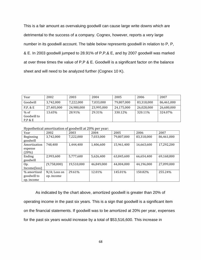
68
This is a fair amount as overvaluing goodwill can cause large write downs which are
detrimental to the success of a company. Cognex, however, reports a very large
number in its goodwill account. The table below represents goodwill in relation to P, P,
& E. In 2003 goodwill jumped to 28.91% of P,P,& E, and by 2007 goodwill was marked
at over three times the value of P,P & E. Goodwill is a significant factor on the balance
sheet and will need to be analyzed further (Cognex 10 K).
Year 2002 2003 2004 2005 2006 2007Goodwill 3,742,000 7,222,000 7,033,000 79,807,000 83,318,000 86,461,000P,P, & E 27,405,000 24,980,000 23,995,000 24,175,000 26,028,000 26,680,000% of Goodwill to P,P & E
13.65% 28.91% 29.31% 330.12% 320.11% 324.07%
Hypothetical amortization of goodwill at 20% per year: Year 2002 2003 2004 2005 2006 2007Beginning goodwill
3,742,000 7,222,000 7,033,000 79,807,000 83,318,000 86,461,000
Amortization expense (20%)
748,400 1,444,400 1,406,600 15,961,400 16,663,600 17,292,200
Ending goodwill
2,993,600 5,777,600 5,626,400 63,845,600 66,654,400 69,168,800
Op. Income(loss)
(9,758,000) 19,510,000 46,849,000 44,004,000 44,196,000 27,099,000
% amortized goodwill to op. income
N/A; Loss on op. income
29.61% 12.01% 145.01% 150.82% 255.24%
As indicated by the chart above, amortized goodwill is greater than 20% of
operating income in the past six years. This is a sign that goodwill is a significant item
on the financial statements. If goodwill was to be amortized at 20% per year, expenses
for the past six years would increase by a total of $53,516,600. This increase in
69
expense will significantly affect net income and shareholder’s equity. Deferring the
expenses brings about the possibility of overstating both accounts.
Research and Development
Scientific and Technical Instruments industry spends large amounts of money on research
and development in hopes of developing new, profitable means of business. According to the
Cognex 10 K, 15.12% of sales revenues were allocated to R&D. The size of the company helps
determine how much money is actually assigned to new projects – the larger the company, the
more money a company can charge to R&D. Cognex reports research and development costs as
expenses until the project proves its technological feasibility. At that time, the product is capitalized
and allocated on the balance sheet (Cognex 10K). There has always been some degree of flexibility
when accounting for research and development activities. It is difficult to determine exactly how
much and where each company spends its R&D allocations, giving companies a chance to hide
potentially unfavorable numbers. Cognex and its competitors all disclose a low to moderate amount
of information regarding R&D. Cognex does disclose that $3,239,000 in 2007 and $3,627,000 2006
were part of a stock‐based compensation expense that was not recorded as R&D in 2005.
The cyclical nature of the industry keeps firms from disclosing exactly where each R&D
dollar is spent. Technology companies do not want other firms to know exactly what they are
developing. Aside from generic statistics like compensation expense adjustments, there is little
disclosure on the details of R&D. This modest disclosure results in low flexibility for firms within
the industry.
70
Foreign Currency
Utilization of a company’s foreign currency risk management program involves
managements’ use of judgment and application of forecasted exchange rates for
forward contacts and other hedging policies. However, reporting and disclosure of
these policies can be somewhat uniform. Using forward contracts can help companies
hedge against changes in exchange rates by setting a future price and exchange rate
that will be transferred. The difference over or under the actual prices that are
exchanged in the future should be reported as a net amount in the current operations
section of the income statement. In regards to the Balance Sheet, asset and liabilities
derivatives can be hedged for current periods. New realization of these amounts can be
adjusted for gains or losses for currency transactions in other comprehensive income.
Adjustments for foreign currency are defined in FASB 133. Discussion and reporting of
foreign subsidiaries’ assets or liability gains or losses are often only reported as a total
in other comprehensive income. FASB Statement 133 and provides compliances in
reporting “hedge accounting”, while FASB 161 illustrates the proper disclosure of
hedging techniques. Other statements provide reporting derivative instruments at fair
value and then the changes in that fair value can be recorded as gains or losses in
other comprehensive income. ( Cognex 10-k). Disclosure of currency risk management
practices MDA and notes of the statements is critical to managements effectiveness in
hedging polices, but because this also provides the risk that management’s disclosures
can be potentially clouted.
The most indebt disclosure of Cognex is the degree to which they use forward
contracts for implementing policies. A forward contract affects accounts receivable
71
because it uses an expected exchange rate as a basis for transactions to occur.
Management’s decisions in these contracts can have an adverse effect on receivables
for the period. Because of potential finger pointing, firms have the potential to disclose
relatively low amounts of information which may not line up with the income statement
and balance sheet.
Governing body requirements provide for the proper disclosure of hedge
accounting techniques; however companies can pick and choose a hedge accounting
preventative measure that they feel will best hedge against foreign currency fluctuation.
Other FASB statements leave room for flexibility in disclosure of a firm’s logic for using
different forms of hedging policies. Relative to industry, Cognex’s logical explanation of
their own hedging techniques is relatively weak.
Evaluating Accounting Strategy
Goodwill
Goodwill is the difference between the acquisition price of a firm and its fair
market value. This premium paid by the parent company is charged on the balance
sheet as an asset. GAAP rules do not allow for goodwill to be amortized, but instead it is
required that the goodwill be tested annually for impairment. Most companies in the
industry carry goodwill but not all of them. Perceptron, for example, operates with zero
goodwill (Perceptron 10k). Those that do make acquisitions often record consistent
debits to the asset account. Managers use these numbers to provide an estimate of the
extra “value” within the firm. These numbers, if not recorded accurately, can distort the
72
true picture of a firms’ operations. Assets can become inflated along with earnings and
equity, misleading investors. The data in the chart below shows goodwill allocations for
firms in the industry. It is apparent that several firms including Cognex, KLA-Tencore,
and Orbotech have all made significant contributions to goodwill recently. This increase
in goodwill comes from acquisitions. “During the fiscal year ended June 30, 2008, the
Company completed its acquisition of ICOS Vision Systems Corporation NV”, which
added $282,569,000 to goodwill (KLA-Tencore 10K). Cognex acquired DVT Corporation
in May 2005 and added nearly $72,774,000 as goodwill (Cognex 10k).
It is difficult to determine the exact value of goodwill, this leaves room for
financial manipulation. Cognex and its competitors disclose ample information regarding
any increases in goodwill. KLA-Tencore provides great detail in explaining the
allocations for all acquisitions. It includes values for intangibles such as existing
technology, customer relationships and brand image (KLA-Tencore 10k). These firms
also test for impairment on an annual basis, per the FASB. Cognex, KLA-Tencore and
Orbotech all report significant increases and no goodwill impairments, implying a
aggressive approach. Showing no impairments suggests a more aggressive accounting
approach is used. This may be attributed to the established value in company assets,
but also indicates a potential red flag. Perceptron and ESIO are conservative in their
accounting for goodwill, showing a very stable value. The amount of disclosure
regarding goodwill for firms in the industry is ample and detailed enough to provide an
accurate description of the extra value a firm may carry.
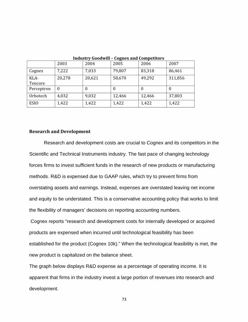
73
Industry Goodwill – Cognex and Competitors
2003 2004 2005 2006 2007 Cognex 7,222 7,033 79,807 83,318 86,461 KLA‐Tencore
20,278 20,621 58,670 49,292 311,856
Perceptron 0 0 0 0 0Orbotech 4,032 9,032 12,466 12,466 37,803 ESIO 1,422 1,422 1,422 1,422 1,422
Research and Development
Research and development costs are crucial to Cognex and its competitors in the
Scientific and Technical Instruments industry. The fast pace of changing technology
forces firms to invest sufficient funds in the research of new products or manufacturing
methods. R&D is expensed due to GAAP rules, which try to prevent firms from
overstating assets and earnings. Instead, expenses are overstated leaving net income
and equity to be understated. This is a conservative accounting policy that works to limit
the flexibility of managers’ decisions on reporting accounting numbers.
Cognex reports “research and development costs for internally developed or acquired
products are expensed when incurred until technological feasibility has been
established for the product (Cognex 10k).” When the technological feasibility is met, the
new product is capitalized on the balance sheet.
The graph below displays R&D expense as a percentage of operating income. It is
apparent that firms in the industry invest a large portion of revenues into research and
development.
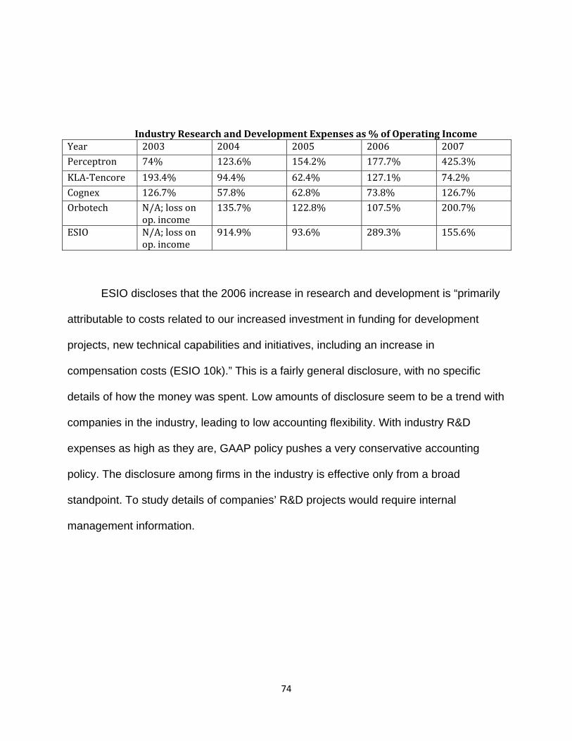
74
Industry Research and Development Expenses as % of Operating Income
Year 2003 2004 2005 2006 2007Perceptron 74% 123.6% 154.2% 177.7% 425.3%KLA‐Tencore 193.4% 94.4% 62.4% 127.1% 74.2%Cognex 126.7% 57.8% 62.8% 73.8% 126.7%Orbotech N/A; loss on
op. income 135.7% 122.8% 107.5% 200.7%
ESIO N/A; loss on op. income
914.9% 93.6% 289.3% 155.6%
ESIO discloses that the 2006 increase in research and development is “primarily
attributable to costs related to our increased investment in funding for development
projects, new technical capabilities and initiatives, including an increase in
compensation costs (ESIO 10k).” This is a fairly general disclosure, with no specific
details of how the money was spent. Low amounts of disclosure seem to be a trend with
companies in the industry, leading to low accounting flexibility. With industry R&D
expenses as high as they are, GAAP policy pushes a very conservative accounting
policy. The disclosure among firms in the industry is effective only from a broad
standpoint. To study details of companies’ R&D projects would require internal
management information.
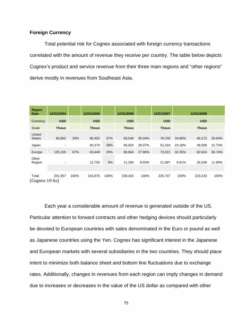
75
Foreign Currency
Total potential risk for Cognex associated with foreign currency transactions
correlated with the amount of revenue they receive per country. The table below depicts
Cognex’s product and service revenue from their three main regions and “other regions”
derive mostly in revenues from Southeast Asia.
Report Date 12/31/2004 12/31/2005 12/31/2006 12/31/2007 12/31/2008
Currency USD USD USD USD USD
Scale Thous Thous Thous Thous Thous
United States 66,802 33% 80,452 37% 83,546 35.04% 78,700 34.86% 66,172 29.64%
Japan - 60,274 28% 66,924 28.07% 52,318 23.18% 48,508 21.73%
Europe 135,155 67% 63,449 29% 66,664 27.96% 73,022 32.35% 82,024 36.74%
Other Region - 12,700 6% 21,290 8.93% 21,697 9.61% 26,539 11.89%
Total 201,957 100% 216,875 100% 238,424 100% 225,737 100% 223,243 100% (Cognex 10‐ks)
Each year a considerable amount of revenue is generated outside of the US.
Particular attention to forward contracts and other hedging devices should particularly
be devoted to European countries with sales denominated in the Euro or pound as well
as Japanese countries using the Yen. Cognex has significant interest in the Japanese
and European markets with several subsidiaries in the two countries. They should place
intent to minimize both balance sheet and bottom line fluctuations due to exchange
rates. Additionally, changes in revenues from each region can imply changes in demand
due to increases or decreases in the value of the US dollar as compared with other
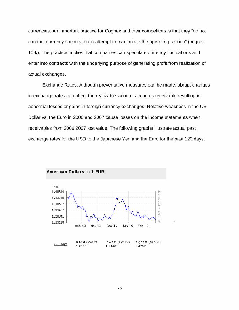
76
currencies. An important practice for Cognex and their competitors is that they “do not
conduct currency speculation in attempt to manipulate the operating section” (cognex
10-k). The practice implies that companies can speculate currency fluctuations and
enter into contracts with the underlying purpose of generating profit from realization of
actual exchanges.
Exchange Rates: Although preventative measures can be made, abrupt changes
in exchange rates can affect the realizable value of accounts receivable resulting in
abnormal losses or gains in foreign currency exchanges. Relative weakness in the US
Dollar vs. the Euro in 2006 and 2007 cause losses on the income statements when
receivables from 2006 2007 lost value. The following graphs illustrate actual past
exchange rates for the USD to the Japanese Yen and the Euro for the past 120 days.
American Dollars to 1 EUR
120 days latest (Mar 2) 1.2596
lowest (Oct 27) 1.2446
highest (Sep 23) 1.4737
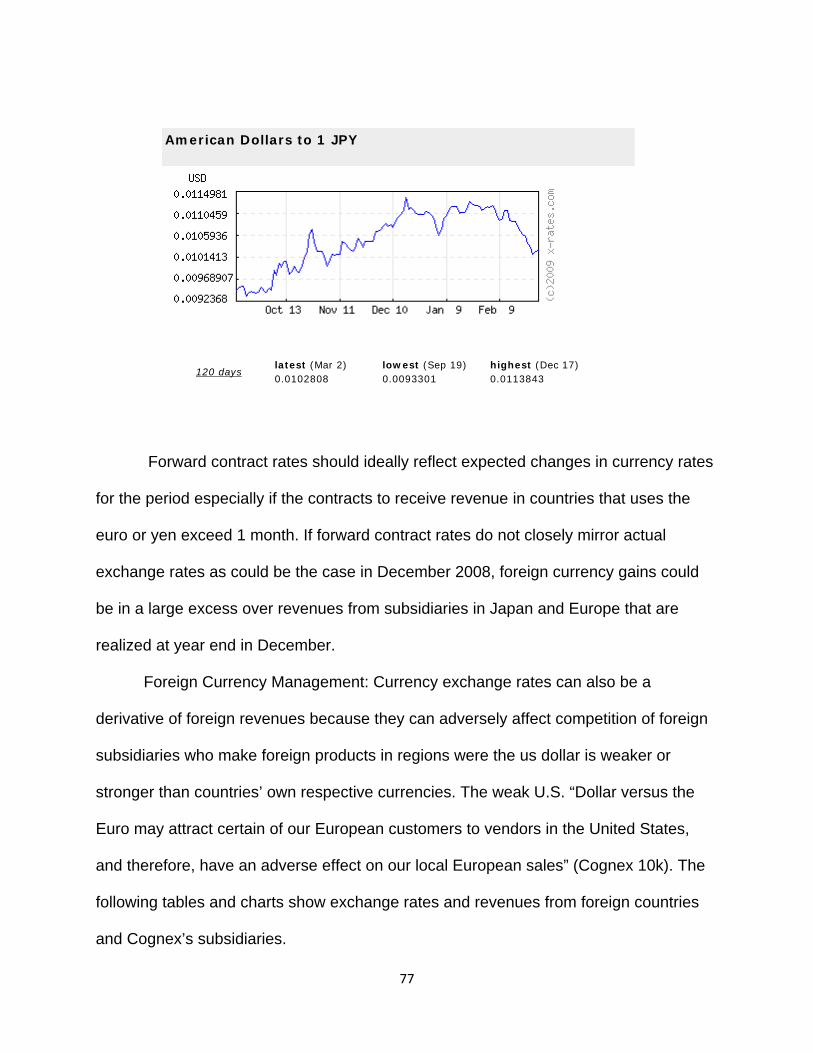
77
Forward contract rates should ideally reflect expected changes in currency rates
for the period especially if the contracts to receive revenue in countries that uses the
euro or yen exceed 1 month. If forward contract rates do not closely mirror actual
exchange rates as could be the case in December 2008, foreign currency gains could
be in a large excess over revenues from subsidiaries in Japan and Europe that are
realized at year end in December.
Foreign Currency Management: Currency exchange rates can also be a
derivative of foreign revenues because they can adversely affect competition of foreign
subsidiaries who make foreign products in regions were the us dollar is weaker or
stronger than countries’ own respective currencies. The weak U.S. “Dollar versus the
Euro may attract certain of our European customers to vendors in the United States,
and therefore, have an adverse effect on our local European sales” (Cognex 10k). The
following tables and charts show exchange rates and revenues from foreign countries
and Cognex’s subsidiaries.
American Dollars to 1 JPY
120 days latest (Mar 2) 0.0102808
lowest (Sep 19) 0.0093301
highest (Dec 17) 0.0113843
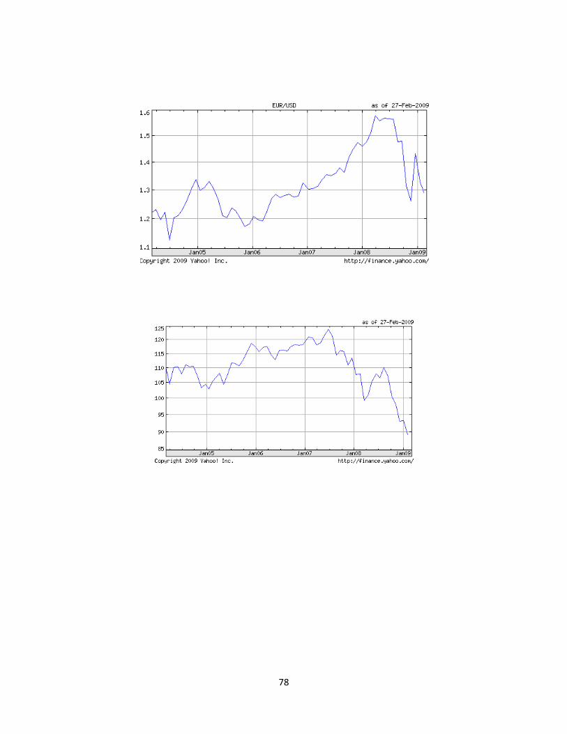
78
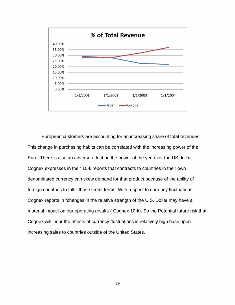
79
European customers are accounting for an increasing share of total revenues.
This change in purchasing habits can be correlated with the increasing power of the
Euro. There is also an adverse effect on the power of the yen over the US dollar.
Cognex expresses in their 10-k reports that contracts to countries in their own
denominated currency can skew demand for that product because of the ability of
foreign countries to fulfill those credit terms. With respect to currency fluctuations,
Cognex reports in “changes in the relative strength of the U.S. Dollar may have a
material impact on our operating results”( Cognex 10-k). So the Potential future risk that
Cognex will incur the effects of currency fluctuations is relatively high base upon
increasing sales to countries outside of the United States.
0.00%
5.00%
10.00%
15.00%
20.00%
25.00%
30.00%
35.00%
40.00%
1/1/2001 1/1/2002 1/1/2003 1/1/2004
% of Total Revenue
Japan Europe
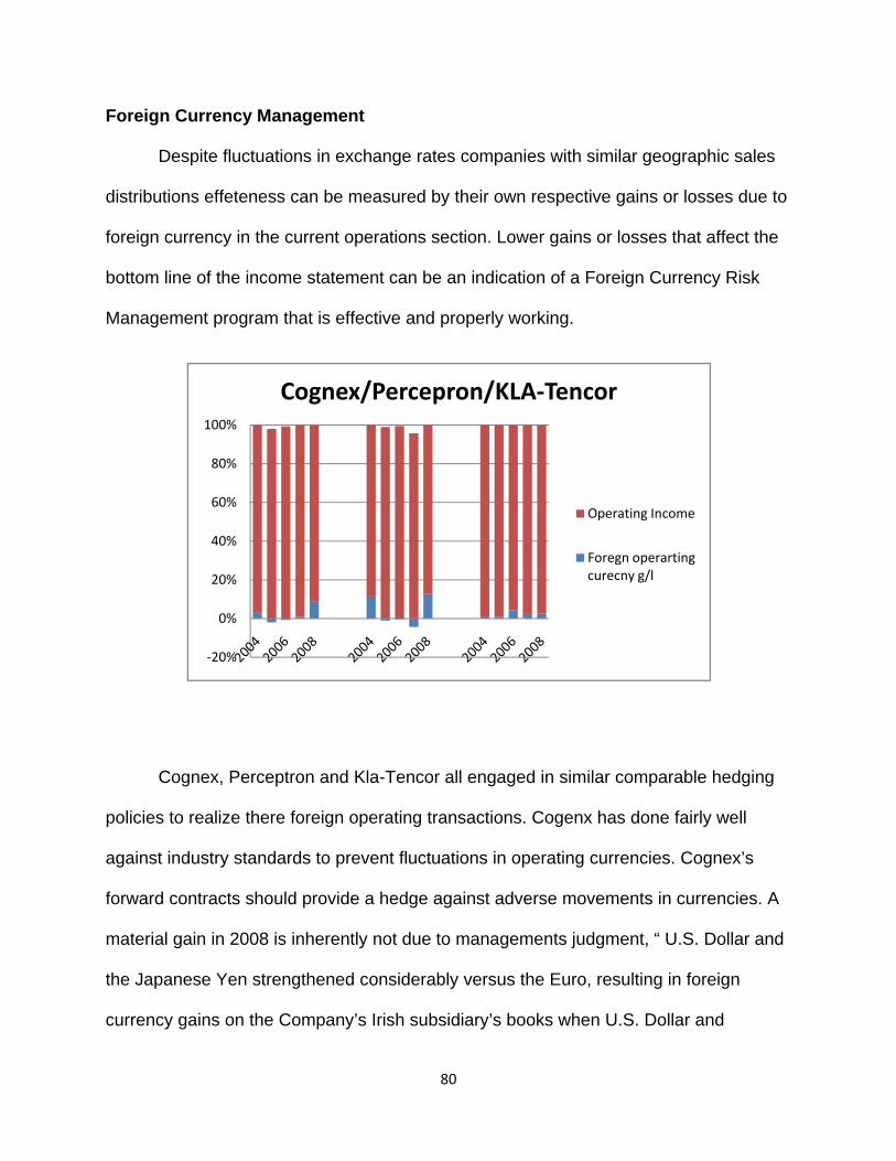
80
Foreign Currency Management
Despite fluctuations in exchange rates companies with similar geographic sales
distributions effeteness can be measured by their own respective gains or losses due to
foreign currency in the current operations section. Lower gains or losses that affect the
bottom line of the income statement can be an indication of a Foreign Currency Risk
Management program that is effective and properly working.
Cognex, Perceptron and Kla-Tencor all engaged in similar comparable hedging
policies to realize there foreign operating transactions. Cogenx has done fairly well
against industry standards to prevent fluctuations in operating currencies. Cognex’s
forward contracts should provide a hedge against adverse movements in currencies. A
material gain in 2008 is inherently not due to managements judgment, “ U.S. Dollar and
the Japanese Yen strengthened considerably versus the Euro, resulting in foreign
currency gains on the Company’s Irish subsidiary’s books when U.S. Dollar and
‐20%
0%
20%
40%
60%
80%
100%
Cognex/Percepron/KLA‐Tencor
Operating Income
Foregn operarting curecny g/l
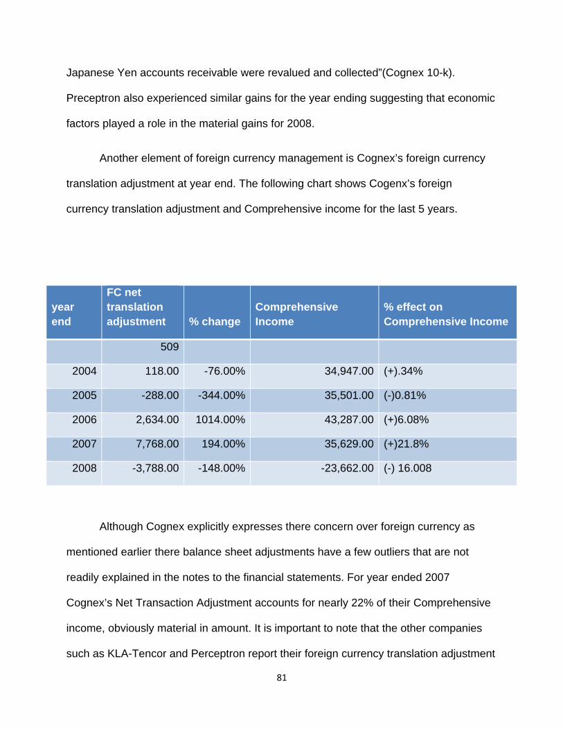
81
Japanese Yen accounts receivable were revalued and collected”(Cognex 10-k).
Preceptron also experienced similar gains for the year ending suggesting that economic
factors played a role in the material gains for 2008.
Another element of foreign currency management is Cognex’s foreign currency
translation adjustment at year end. The following chart shows Cogenx’s foreign
currency translation adjustment and Comprehensive income for the last 5 years.
Although Cognex explicitly expresses there concern over foreign currency as
mentioned earlier there balance sheet adjustments have a few outliers that are not
readily explained in the notes to the financial statements. For year ended 2007
Cognex’s Net Transaction Adjustment accounts for nearly 22% of their Comprehensive
income, obviously material in amount. It is important to note that the other companies
such as KLA-Tencor and Perceptron report their foreign currency translation adjustment
year end
FC net translation adjustment % change
Comprehensive Income
% effect on Comprehensive Income
509
2004 118.00 -76.00% 34,947.00 (+).34%
2005 -288.00 -344.00% 35,501.00 (-)0.81%
2006 2,634.00 1014.00% 43,287.00 (+)6.08%
2007 7,768.00 194.00% 35,629.00 (+)21.8%
2008 -3,788.00 -148.00% -23,662.00 (-) 16.008
82
and the effect of their “hedging” transactions as a reduction or gain to the Translation
adjustment. Cognex however reports this amount net of hedging adjustment and
provides little disclosure on this account.
Quality of Disclosure
Introduction
An intricate piece in the accounting analysis process is the evaluation of the quality of
disclosure. The general accounting regulations require a minimal level of disclosure, ultimately
entrusting management with the decision making of financial disclosure. Managers are
assigned the task of determining what information to include and to what extent to include the
information within the financial statements. Management must decide how much information to
disclose without giving away their competitive advantages while still providing enough
information to give a clear definition of the firm’s economic performance. Quality of disclosure
becomes an important element in the overall presentation of a firm’s accounting records.
Goodwill
Accounting policies for recording good will are important for this industry because
carried amount of good will for a company can essentially overstate reported assets.
The company reports goodwill in two primary categories Modular Visual Systems
Division (MVDS) and Surface Inspection Systems Division (SISD). Overall the
company overstates its goodwill by failing to write it down by adequate amounts each
year. Though the amount of goodwill write offs each year is not at a substantial amount,
the company does write off for the impairment of goodwill. The company states goodwill
83
at cost and assesses potential impairments as the year goes on. Part of Cognex’s
business strategy includes:
“Selective expansion into new machine vision applications
through the acquisition of businesses and technologies.” (Cognex 10-k)
Cognex discloses proper discussion of their uses of GAAP for impairing goodwill
and other intangible assets in the management discussion and analysis section. The
notes to the financial statements provide satisfactory information on the acquisition
history of the business and the exact amount that was capitalized into goodwill for each
acquisition. Goodwill saw a large increase in 2005 due to the company’s largest
acquisition with the purchase of DVT Corporation. DVT Corporation was a vision
technology leader in R&D, which provided a large increase in the functionality of
Cognex. Cognex’s consolidated balance sheet reports the amount of good will for 2007
at 86,461 million. Accompanied by the large amount of goodwill is a suitable amount of
disclosure in the notes to the financial statements. Additionally each division’s goodwill
amounts are clearly separated. Cognex fails to supplement its consolidated amount of
goodwill with proper logic and reasoning for such an aggressive accounting approach.
Planned amortization schedules of goodwill from acquisitions is supplied in the notes to
the financial statements. The Company provides a mid to moderately high level of
information pertaining to its goodwill accounts and policies.
84
Research and Development
Cognex does not release a high level of disclosure with regard to research and
development. Cognex, being in a technologically advanced field of operation, has found
it beneficial to release only a limited amount of information in the area of R&D. The
company provided very little explanation of R&D in the notes to consolidated financial
statements. A high level of disclosure in the R&D section could prove to be a threat to
the company’s competitive advantage. The 10-K effectively describes the area of R&D
by stating “Research and development costs for internally-developed or acquired
products are expensed when incurred until technological feasibility has been
established for the product” (Cognex 10-K). A large increase in R&D between 2005 and
2006 is attributed to the acquisition of DVT in May of 2005 resulting in increased
engineering personnel, and a stock-based compensation expense classified as an R&D
expense. The level of disclosure is relatively low considering the significance of R&D in
the company.
Foreign Currency
Cognex provides a high level of disclosure when discussing its foreign currency
risks. The company openly discusses how an unanticipated change in foreign currency
markets could have an adverse effect on the company’s earnings. The accounting
treatment for accounts gain or loss due to foreign currency is disclosed in the notes to
the financial statements. The Cognex 10-K goes into more detail when it explains that,”
the Company could experience unanticipated foreign currency gains or losses that
could have a material impact on the Company’s results of operations” (Cognex 10-K).
85
Cognex explains its method in hedging to prevent any anticipated currency risks that it
may face. Additionally Cognex’s “Disclosures About Market Risks” discuses their risk
management practices in using future contacts to hedge against fluctuations in foreign
currency. The company clearly states that the level of success in its foreign currency
risk management program is dependant primarily on its ability to accurately forecast
volatility in the currency markets in which it is involved. The Cognex 10-K provides a
large amount of disclosure when discussing its foreign currency risks.
Cognex’s disclosure of key risk management and hedging policies is relatively
low in comparison to industry. Cognex Corporation’s Consolidated Statement of
Operations clearly discloses their foreign currency gain or loss for the respective year
ended. The accounting treatment for gain or loss due to foreign currency is disclosed in
the notes to the finical statements, but fails to disclose quantitative information on
forward contracts to hedge these accounts. According to Cognex’s 10-k, exchange
rate fluctuations are adjusted annually due to the value of the assets and liabilities held
by subsidiaries fluctuate. Treatment for these exchange rate fluctuations is disclosed in
the notes following “Comprehensive income”. However, the total assets and liabilities of
their subsidiaries in Japan and Ireland are not readily disclosed. In addition, hedging
effects on comprehensive income are reported net of this effect rather than separately.
Cognex provides enough information in the financial statements accompanied by the
notes and disclosures to provide enough information for a year ended analysis of gains
and losses, but lack of discloser in the notes makes it difficult to analyze management’s
logic.
86
Conclusion
The quality of any firms’ financial statements is dependent upon the amount of
information management decides to disclose. The more information given by the
management in the footnotes and explanations of the firms’ activity, the more valuable
the financial statements are to those analyzing them. Cognex goes into superior detail
in describing their business activities through the utilization of supplemental data where
necessary. After analyzing management’s discussions and disclosure of important
information we can ultimately determine that Cognex provides a moderate level of
quality in their company disclosure.
Quantitative Analysis
Quantitative analysis of a firm involves studying ratios within the financial
statements to get a true picture of the underlying economic activity of the firm. As with
all other data, there is room for manipulation and distortion when reporting the
diagnostics. This is why it is important to be cautious when analyzing numbers, and
identify red flags when able. The ratios will help analysts to identify possible distortions
and estimate a true value of the firm. Two types of ratio diagnostics that are often used
are (1)revenue manipulation and (2)expense manipulation diagnostics. These ratios
cannot be used effectively by themselves, but when consolidated and analyzed they are
very useful in determining business efficiency.
87
Revenue Manipulation Diagnostics
Net sales/cash from sales
This ratio is calculated by dividing net sales by cash from sales, allowing for an
analysis of the firms documented sales figure. The figure also provides analysts with an
amount of cash the firm collects in comparison to total sales during the period, informing
on a firms ability to meet short term liabilities. Firms also desire for an average around
one because when the firm sells the product they want to receive payment in
accordance. As opposed to expressing that revenue in accounts receivable that could
result as an allowance for doubtful accounts.
When calculating the ratio most firms should produce a figure of one or greater than
one. If the ratio varies from year to year the accounting policy used by the firm could be
questioned and a potential red flag may need to be raised.
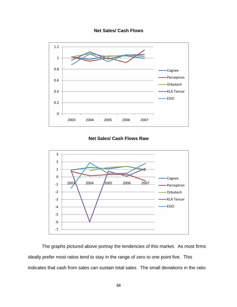
88
Net Sales/ Cash Flows
Net Sales/ Cash Flows Raw
The graphs pictured above portray the tendencies of this market. As most firms
ideally prefer most ratios tend to stay in the range of zero to one point five. This
indicates that cash from sales can sustain total sales. The small deviations in the ratio
0
0.2
0.4
0.6
0.8
1
1.2
2003 2004 2005 2006 2007
Cognex
Perceptron
Orbotech
KLA Tencor
ESIO
‐7
‐6
‐5
‐4
‐3
‐2
‐1
0
1
2
3
2003 2004 2005 2006 2007Cognex
Perceptron
Orbotech
KLA Tencor
ESIO
89
can most often be clarified by changes in total sales from year to year. For instance in
KLA Tencor’s case sales increase 39 percent from 2004 to 2005, thus ruling out the
potential for a red flag. In evaluation of the overall industry one can conclude that
Cognex is in line with the industry as a whole with an acceptable level of disclosure.
Additionally from an investors viewpoint it demonstrates that the firms have a good
buyer seller relationship and receive a quick cash payment, and experience only a few if
any doubtful accounts.
Net sales/Accounts Receivable
Net sales/Accounts Receivable is a ratio that evaluates the amount of net sales
of a firm to the amount of sales purchased on credit. In the scientific instruments
industry, the amount of credit sales could be potentially high because of the expensive
price of the products. However these high ratios are not ideal in comparison to cash
collection and meeting short term liabilities. Additionally instead of that cash sitting in
an account gaining interest, it results in a interest free loan for the client. High ratios
result either a good collection of cash or that the industry mainly makes sales in cash. It
also indicates a highly liquid firm capable of meeting short term obligations. A low ratio
in the industry in comparison to the others could indicate the need for a change in the
firm’s collection policy.
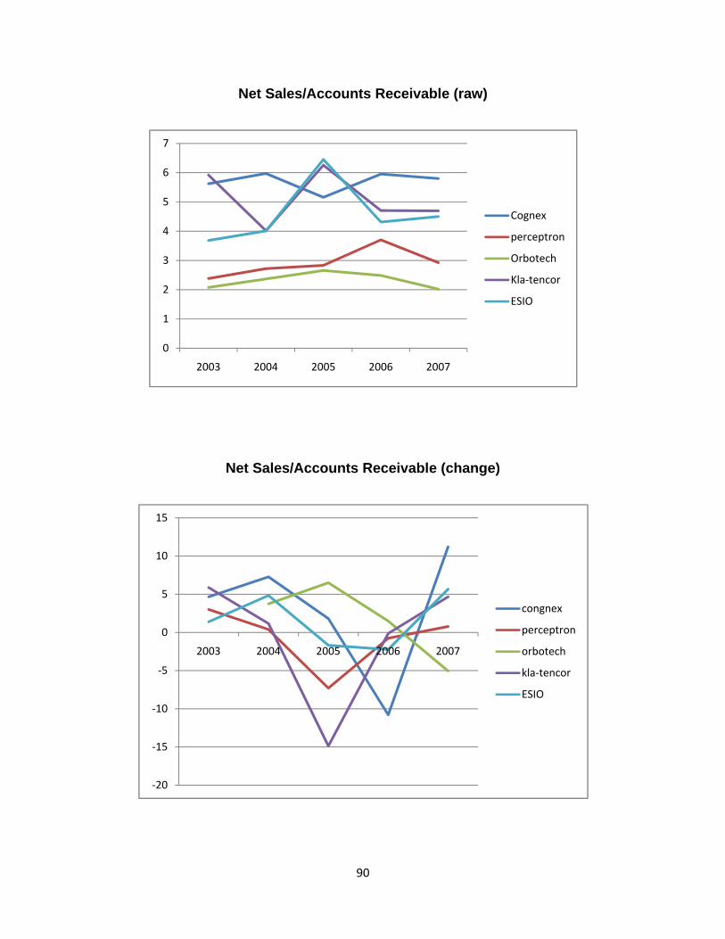
90
Net Sales/Accounts Receivable (raw)
Net Sales/Accounts Receivable (change)
0
1
2
3
4
5
6
7
2003 2004 2005 2006 2007
Cognex
perceptron
Orbotech
Kla‐tencor
ESIO
‐20
‐15
‐10
‐5
0
5
10
15
2003 2004 2005 2006 2007
congnex
perceptron
orbotech
kla‐tencor
ESIO
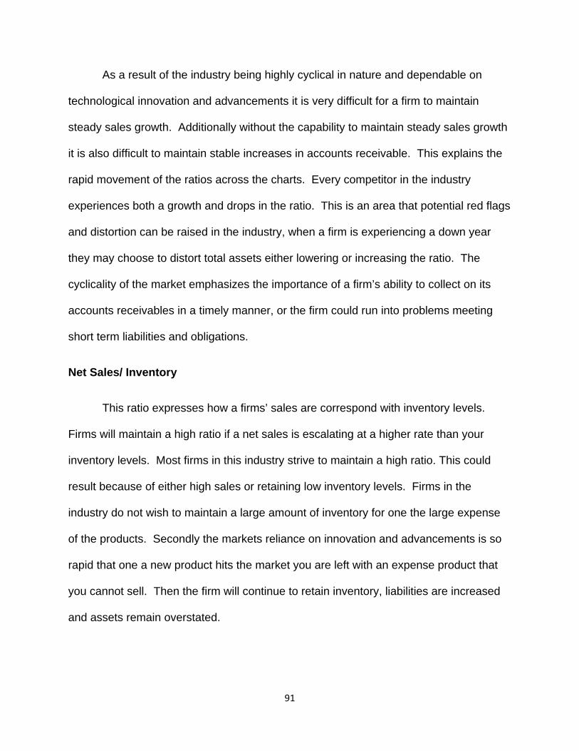
91
As a result of the industry being highly cyclical in nature and dependable on
technological innovation and advancements it is very difficult for a firm to maintain
steady sales growth. Additionally without the capability to maintain steady sales growth
it is also difficult to maintain stable increases in accounts receivable. This explains the
rapid movement of the ratios across the charts. Every competitor in the industry
experiences both a growth and drops in the ratio. This is an area that potential red flags
and distortion can be raised in the industry, when a firm is experiencing a down year
they may choose to distort total assets either lowering or increasing the ratio. The
cyclicality of the market emphasizes the importance of a firm’s ability to collect on its
accounts receivables in a timely manner, or the firm could run into problems meeting
short term liabilities and obligations.
Net Sales/ Inventory
This ratio expresses how a firms’ sales are correspond with inventory levels.
Firms will maintain a high ratio if a net sales is escalating at a higher rate than your
inventory levels. Most firms in this industry strive to maintain a high ratio. This could
result because of either high sales or retaining low inventory levels. Firms in the
industry do not wish to maintain a large amount of inventory for one the large expense
of the products. Secondly the markets reliance on innovation and advancements is so
rapid that one a new product hits the market you are left with an expense product that
you cannot sell. Then the firm will continue to retain inventory, liabilities are increased
and assets remain overstated.
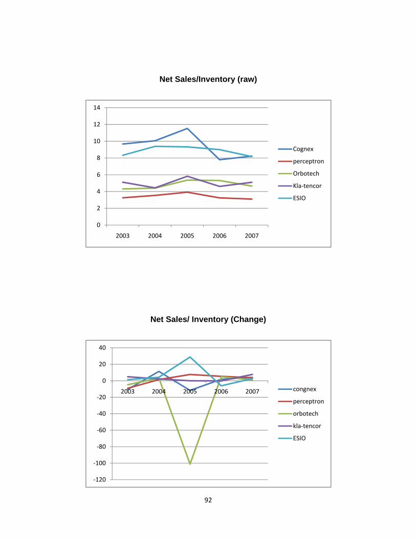
92
Net Sales/Inventory (raw)
Net Sales/ Inventory (Change)
0
2
4
6
8
10
12
14
2003 2004 2005 2006 2007
Cognex
perceptron
Orbotech
Kla‐tencor
ESIO
‐120
‐100
‐80
‐60
‐40
‐20
0
20
40
2003 2004 2005 2006 2007 congnex
perceptron
orbotech
kla‐tencor
ESIO
93
From the adjusted chart you can gain a in depth view of the unpredictability of the
market. All firms in the market continue to have both times of increasing ratios, followed
by a down turn and a period of decreasing. This is all stimulated by the ability of the
firm to produce new innovated products in accordance with firms across the industry.
From the chart you can see Orbotech struggled in the market from 2004 to 2006.
However by increasing research and development costs was able to bring them out of
the hole and reclaim their share of the market. No potential red flags should be raised,
on part of the cyclicality. It is normal in the field for firms to experience times of high
sales with low inventory levels insinuating a time of new innovation or advancement.
Followed by times of low sales with high inventory levels suggesting a time of low sales
with high inventory levels and a competitor introducing a new innovation to the market.
Net sales/warranty expenses
The net sales to warranty expense ratio shows the amount of sales in
comparison to warranty expenses for a firm. This ratio is valuable because the amount
of sales in a period is used to cover the warranty expense costs. Warranty expenses
are the direct result of product failure. Firms want to experience a high ratio which would
indicate large sales or low warranty expenses with respect to one another. Cognex is
the only firm in the industry to disclose their amount of warranty expense each year.
This makes it difficult to determine how Cognex is performing compared its competitors.
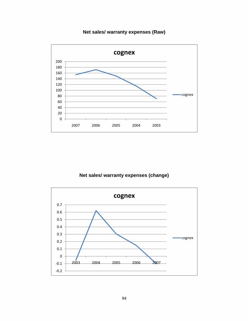
94
Net sales/ warranty expenses (Raw)
Net sales/ warranty expenses (change)
020406080100120140160180200
2007 2006 2005 2004 2003
cognex
cognex
‐0.2
‐0.1
0
0.1
0.2
0.3
0.4
0.5
0.6
0.7
2003 2004 2005 2006 2007
cognex
cognex
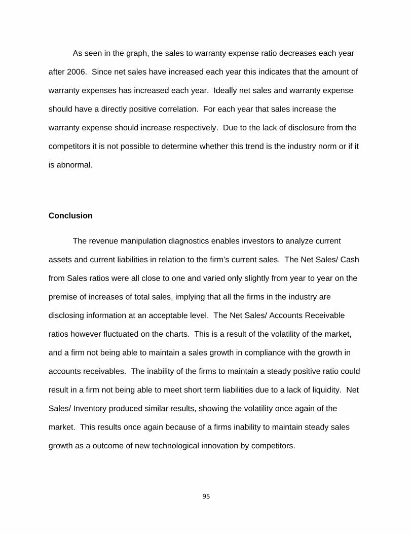
95
As seen in the graph, the sales to warranty expense ratio decreases each year
after 2006. Since net sales have increased each year this indicates that the amount of
warranty expenses has increased each year. Ideally net sales and warranty expense
should have a directly positive correlation. For each year that sales increase the
warranty expense should increase respectively. Due to the lack of disclosure from the
competitors it is not possible to determine whether this trend is the industry norm or if it
is abnormal.
Conclusion
The revenue manipulation diagnostics enables investors to analyze current
assets and current liabilities in relation to the firm’s current sales. The Net Sales/ Cash
from Sales ratios were all close to one and varied only slightly from year to year on the
premise of increases of total sales, implying that all the firms in the industry are
disclosing information at an acceptable level. The Net Sales/ Accounts Receivable
ratios however fluctuated on the charts. This is a result of the volatility of the market,
and a firm not being able to maintain a sales growth in compliance with the growth in
accounts receivables. The inability of the firms to maintain a steady positive ratio could
result in a firm not being able to meet short term liabilities due to a lack of liquidity. Net
Sales/ Inventory produced similar results, showing the volatility once again of the
market. This results once again because of a firms inability to maintain steady sales
growth as a outcome of new technological innovation by competitors.
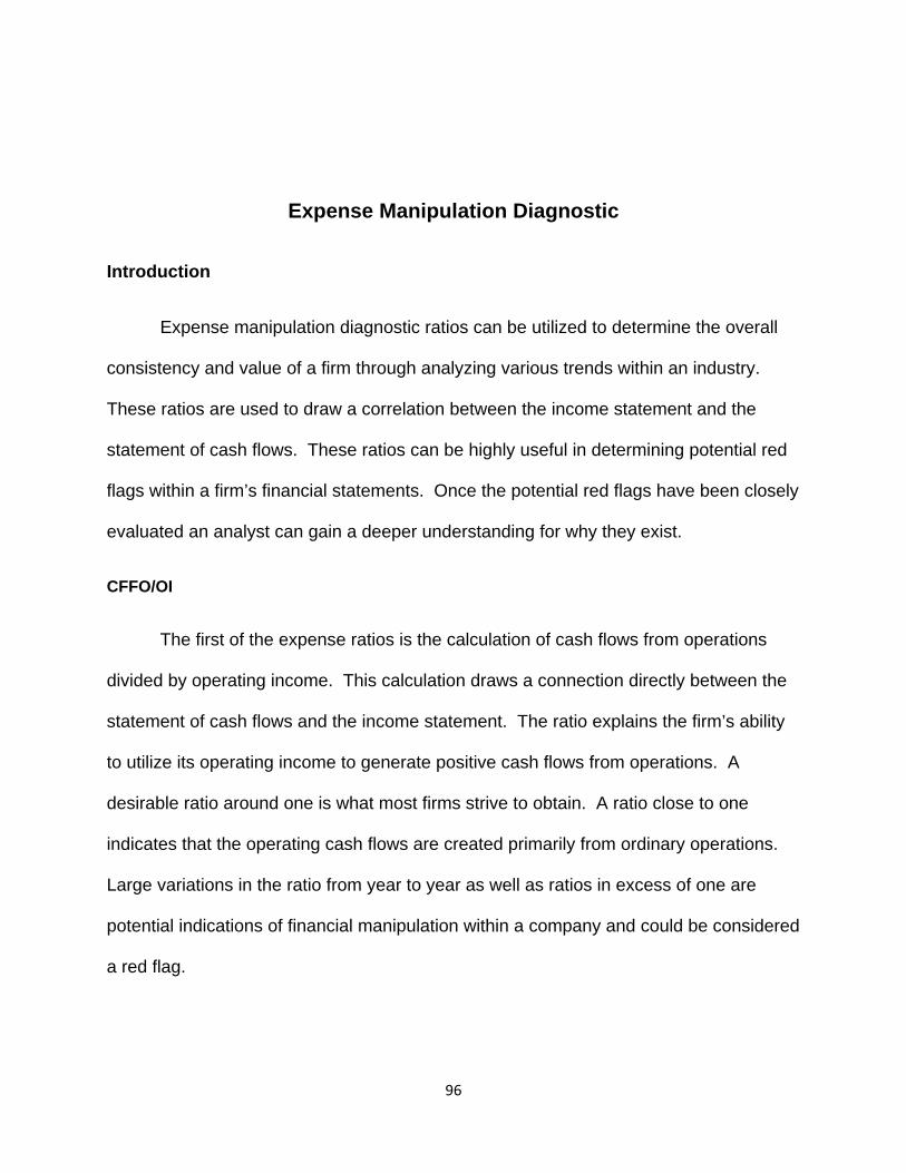
96
Expense Manipulation Diagnostic
Introduction
Expense manipulation diagnostic ratios can be utilized to determine the overall
consistency and value of a firm through analyzing various trends within an industry.
These ratios are used to draw a correlation between the income statement and the
statement of cash flows. These ratios can be highly useful in determining potential red
flags within a firm’s financial statements. Once the potential red flags have been closely
evaluated an analyst can gain a deeper understanding for why they exist.
CFFO/OI
The first of the expense ratios is the calculation of cash flows from operations
divided by operating income. This calculation draws a connection directly between the
statement of cash flows and the income statement. The ratio explains the firm’s ability
to utilize its operating income to generate positive cash flows from operations. A
desirable ratio around one is what most firms strive to obtain. A ratio close to one
indicates that the operating cash flows are created primarily from ordinary operations.
Large variations in the ratio from year to year as well as ratios in excess of one are
potential indications of financial manipulation within a company and could be considered
a red flag.
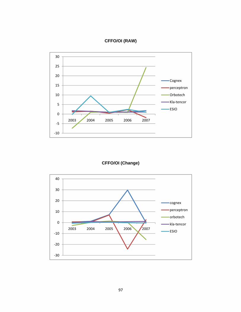
97
CFFO/OI (RAW)
CFFO/OI (Change)
‐10
‐5
0
5
10
15
20
25
30
2003 2004 2005 2006 2007
Cognex
perceptron
Orbotech
Kla‐tencor
ESIO
‐30
‐20
‐10
0
10
20
30
40
2003 2004 2005 2006 2007
cognex
perceptron
orbotech
kla‐tencor
ESIO
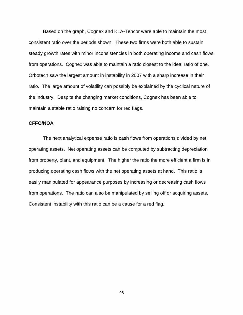
98
Based on the graph, Cognex and KLA-Tencor were able to maintain the most
consistent ratio over the periods shown. These two firms were both able to sustain
steady growth rates with minor inconsistencies in both operating income and cash flows
from operations. Cognex was able to maintain a ratio closest to the ideal ratio of one.
Orbotech saw the largest amount in instability in 2007 with a sharp increase in their
ratio. The large amount of volatility can possibly be explained by the cyclical nature of
the industry. Despite the changing market conditions, Cognex has been able to
maintain a stable ratio raising no concern for red flags.
CFFO/NOA
The next analytical expense ratio is cash flows from operations divided by net
operating assets. Net operating assets can be computed by subtracting depreciation
from property, plant, and equipment. The higher the ratio the more efficient a firm is in
producing operating cash flows with the net operating assets at hand. This ratio is
easily manipulated for appearance purposes by increasing or decreasing cash flows
from operations. The ratio can also be manipulated by selling off or acquiring assets.
Consistent instability with this ratio can be a cause for a red flag.
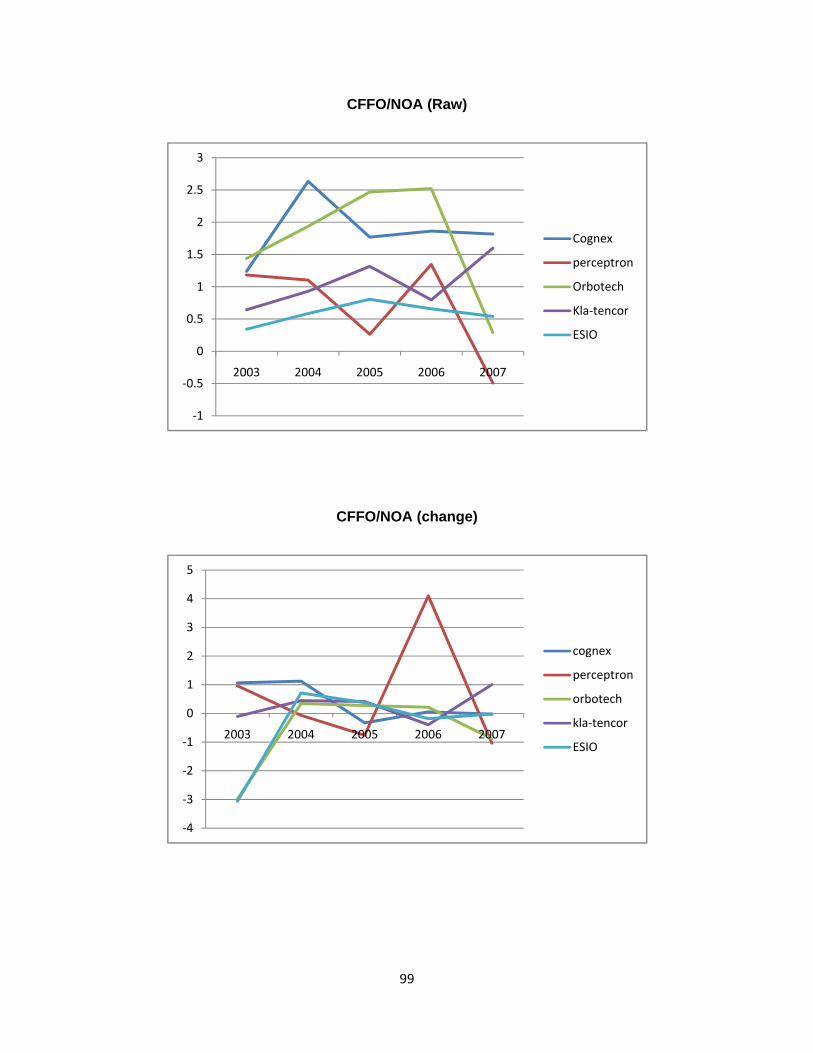
99
CFFO/NOA (Raw)
CFFO/NOA (change)
‐1
‐0.5
0
0.5
1
1.5
2
2.5
3
2003 2004 2005 2006 2007
Cognex
perceptron
Orbotech
Kla‐tencor
ESIO
‐4
‐3
‐2
‐1
0
1
2
3
4
5
2003 2004 2005 2006 2007
cognex
perceptron
orbotech
kla‐tencor
ESIO
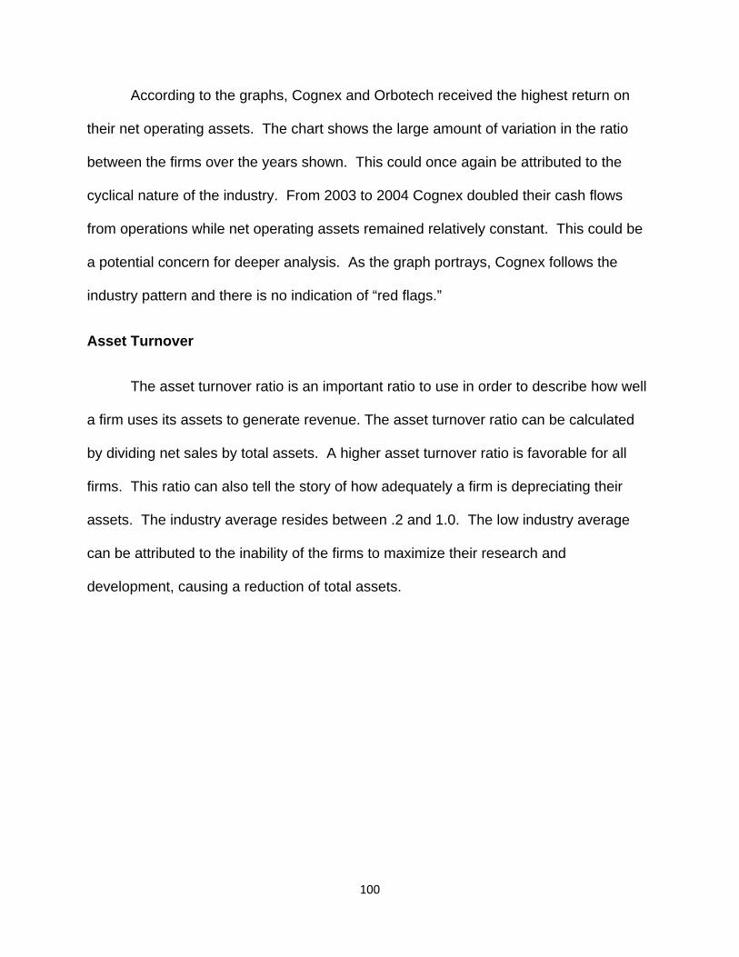
100
According to the graphs, Cognex and Orbotech received the highest return on
their net operating assets. The chart shows the large amount of variation in the ratio
between the firms over the years shown. This could once again be attributed to the
cyclical nature of the industry. From 2003 to 2004 Cognex doubled their cash flows
from operations while net operating assets remained relatively constant. This could be
a potential concern for deeper analysis. As the graph portrays, Cognex follows the
industry pattern and there is no indication of “red flags.”
Asset Turnover
The asset turnover ratio is an important ratio to use in order to describe how well
a firm uses its assets to generate revenue. The asset turnover ratio can be calculated
by dividing net sales by total assets. A higher asset turnover ratio is favorable for all
firms. This ratio can also tell the story of how adequately a firm is depreciating their
assets. The industry average resides between .2 and 1.0. The low industry average
can be attributed to the inability of the firms to maximize their research and
development, causing a reduction of total assets.
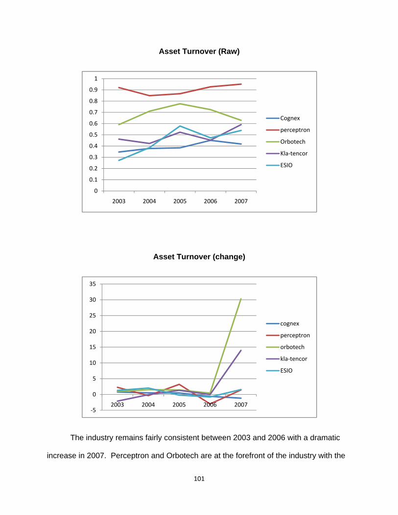
101
Asset Turnover (Raw)
Asset Turnover (change)
The industry remains fairly consistent between 2003 and 2006 with a dramatic
increase in 2007. Perceptron and Orbotech are at the forefront of the industry with the
0
0.1
0.2
0.3
0.4
0.5
0.6
0.7
0.8
0.9
1
2003 2004 2005 2006 2007
Cognex
perceptron
Orbotech
Kla‐tencor
ESIO
‐5
0
5
10
15
20
25
30
35
2003 2004 2005 2006 2007
cognex
perceptron
orbotech
kla‐tencor
ESIO
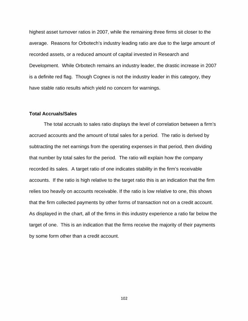
102
highest asset turnover ratios in 2007, while the remaining three firms sit closer to the
average. Reasons for Orbotech’s industry leading ratio are due to the large amount of
recorded assets, or a reduced amount of capital invested in Research and
Development. While Orbotech remains an industry leader, the drastic increase in 2007
is a definite red flag. Though Cognex is not the industry leader in this category, they
have stable ratio results which yield no concern for warnings.
Total Accruals/Sales
The total accruals to sales ratio displays the level of correlation between a firm’s
accrued accounts and the amount of total sales for a period. The ratio is derived by
subtracting the net earnings from the operating expenses in that period, then dividing
that number by total sales for the period. The ratio will explain how the company
recorded its sales. A target ratio of one indicates stability in the firm’s receivable
accounts. If the ratio is high relative to the target ratio this is an indication that the firm
relies too heavily on accounts receivable. If the ratio is low relative to one, this shows
that the firm collected payments by other forms of transaction not on a credit account.
As displayed in the chart, all of the firms in this industry experience a ratio far below the
target of one. This is an indication that the firms receive the majority of their payments
by some form other than a credit account.
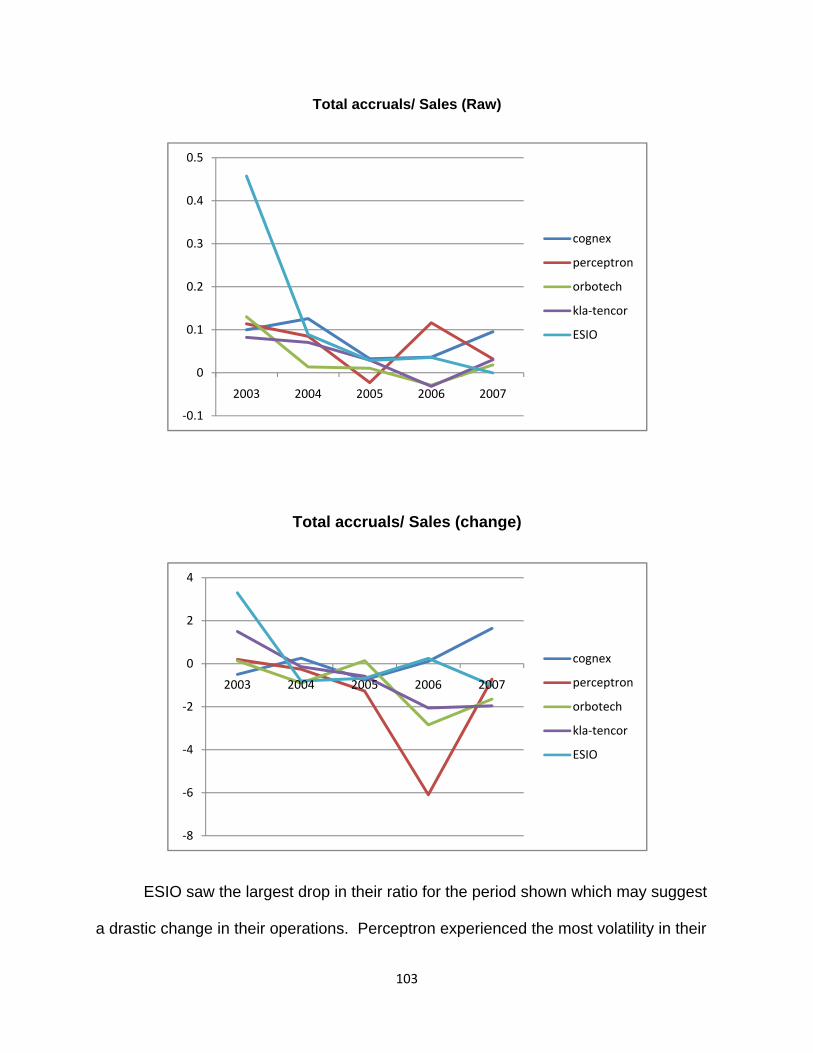
103
Total accruals/ Sales (Raw)
Total accruals/ Sales (change)
ESIO saw the largest drop in their ratio for the period shown which may suggest
a drastic change in their operations. Perceptron experienced the most volatility in their
‐0.1
0
0.1
0.2
0.3
0.4
0.5
2003 2004 2005 2006 2007
cognex
perceptron
orbotech
kla‐tencor
ESIO
‐8
‐6
‐4
‐2
0
2
4
2003 2004 2005 2006 2007
cognex
perceptron
orbotech
kla‐tencor
ESIO
104
ratio from year to year with a large negative change in 2006. Cognex saw the highest
level of consistency throughout the period. Despite a small decrease between 2004
and 2005, Cognex remains slightly higher than its competitors with respect to the
accruals to sales ratio. Cognex had no unusual fluctuations in their ratio which indicates
the absences of “red flags”.
Potential Red Flags/Undo Accounting Distortions
The Federal Accounting Standards Board has implemented that specific criteria
be met when disclosing financial statements. These standards were put in place to help
investors get a clear picture of company operations. As mentioned previously, it is
know that managers often have a final say in the level of disclosure in the financial
statements. The greater the level of disclosure, the more credible a company will look
from an investor standpoint. If numbers do not seem to be in order, it may bring about a
red flag. A red flag is used to indicate possible distortions in accounting policies.
Cogenx has two areas needing greater analysis: Research and Development, and
Goodwill.
Research and Development
Since Cognex invest large amounts of capital in research and development, we
have determined that R&D should be recorded as an asset rather than an expense. We
have decided that we should capitalize 80% of research and development as an asset
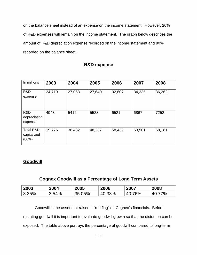
105
on the balance sheet instead of an expense on the income statement. However, 20%
of R&D expenses will remain on the income statement. The graph below describes the
amount of R&D depreciation expense recorded on the income statement and 80%
recorded on the balance sheet.
R&D expense
Goodwill
Cognex Goodwill as a Percentage of Long Term Assets
2003 2004 2005 2006 2007 2008 3.35% 3.54% 35.05% 40.33% 40.76% 40.77%
Goodwill is the asset that raised a “red flag” on Cognex’s financials. Before
restating goodwill it is important to evaluate goodwill growth so that the distortion can be
exposed. The table above portrays the percentage of goodwill compared to long-term
In millions 2003 2004 2005 2006 2007 2008
R&D expense
24,719 27,063 27,640 32,607 34,335 36,262
R&D depreciation expense
4943
5412
5528
6521
6867
7252
Total R&D capitalized (80%)
19,776 36,482 48,237 58,439 63,501 68,181
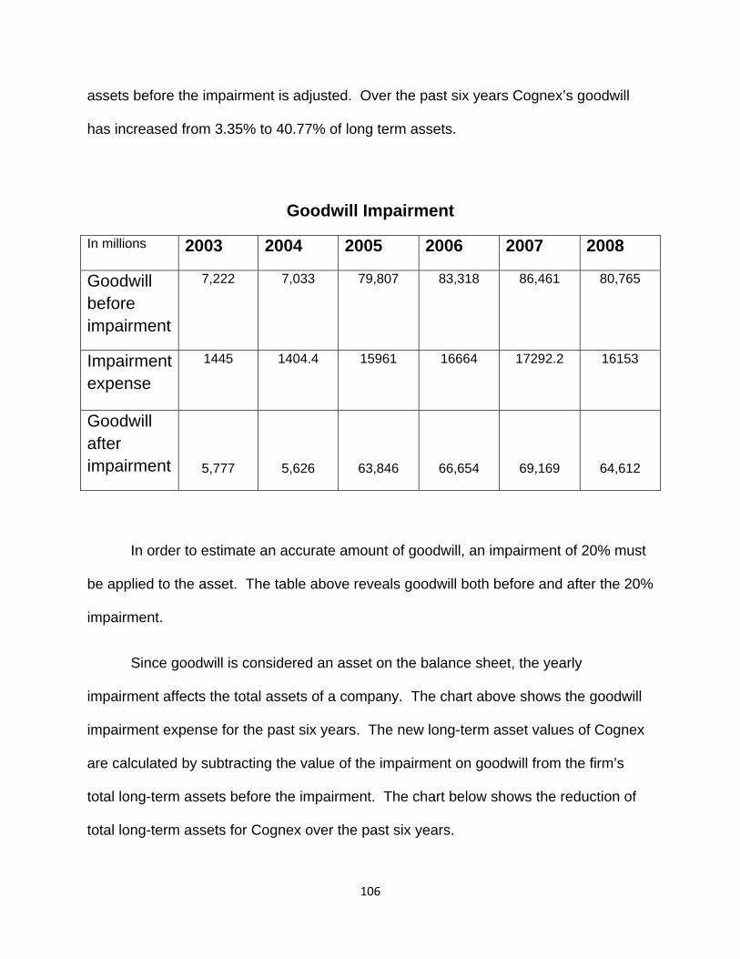
106
assets before the impairment is adjusted. Over the past six years Cognex’s goodwill
has increased from 3.35% to 40.77% of long term assets.
Goodwill Impairment
In millions 2003 2004 2005 2006 2007 2008
Goodwill before impairment
7,222 7,033 79,807 83,318 86,461 80,765
Impairment expense
1445
1404.4
15961
16664
17292.2
16153
Goodwill after impairment 5,777 5,626 63,846 66,654 69,169 64,612
In order to estimate an accurate amount of goodwill, an impairment of 20% must
be applied to the asset. The table above reveals goodwill both before and after the 20%
impairment.
Since goodwill is considered an asset on the balance sheet, the yearly
impairment affects the total assets of a company. The chart above shows the goodwill
impairment expense for the past six years. The new long-term asset values of Cognex
are calculated by subtracting the value of the impairment on goodwill from the firm’s
total long-term assets before the impairment. The chart below shows the reduction of
total long-term assets for Cognex over the past six years.
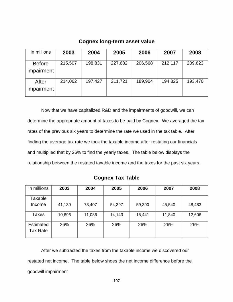
107
Cognex long-term asset value
In millions 2003 2004 2005 2006 2007 2008
Before impairment
215,507 198,831 227,682 206,568 212,117 209,623
After impairment
214,062 197,427 211,721 189,904 194,825 193,470
Now that we have capitalized R&D and the impairments of goodwill, we can
determine the appropriate amount of taxes to be paid by Cognex. We averaged the tax
rates of the previous six years to determine the rate we used in the tax table. After
finding the average tax rate we took the taxable income after restating our financials
and multiplied that by 26% to find the yearly taxes. The table below displays the
relationship between the restated taxable income and the taxes for the past six years.
Cognex Tax Table
In millions 2003 2004 2005 2006 2007 2008
Taxable Income 41,139 73,407 54,397 59,390 45,540 48,483
Taxes 10,696 11,086 14,143 15,441 11,840 12,606
Estimated Tax Rate
26% 26% 26% 26% 26% 26%
After we subtracted the taxes from the taxable income we discovered our
restated net income. The table below shoes the net income difference before the
goodwill impairment
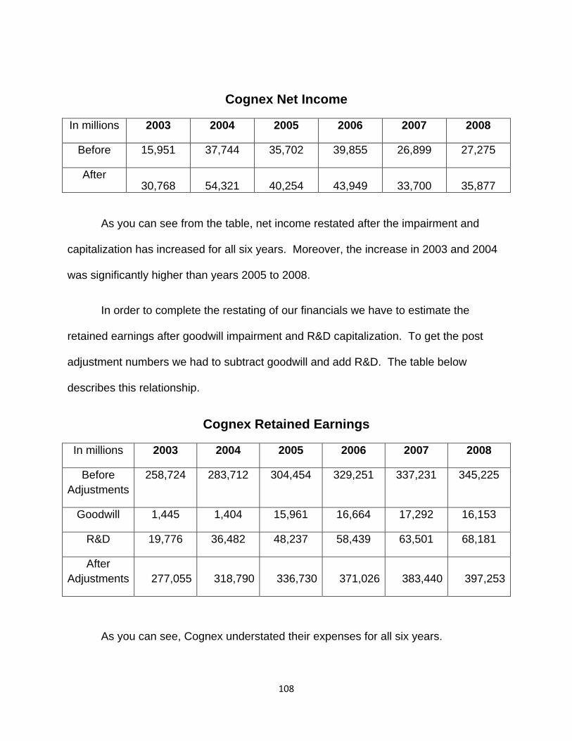
108
Cognex Net Income
In millions 2003 2004 2005 2006 2007 2008
Before 15,951 37,744 35,702 39,855 26,899 27,275
After 30,768 54,321 40,254 43,949 33,700 35,877
As you can see from the table, net income restated after the impairment and
capitalization has increased for all six years. Moreover, the increase in 2003 and 2004
was significantly higher than years 2005 to 2008.
In order to complete the restating of our financials we have to estimate the
retained earnings after goodwill impairment and R&D capitalization. To get the post
adjustment numbers we had to subtract goodwill and add R&D. The table below
describes this relationship.
Cognex Retained Earnings
In millions 2003 2004 2005 2006 2007 2008
Before Adjustments
258,724 283,712 304,454 329,251 337,231 345,225
Goodwill 1,445 1,404 15,961 16,664 17,292 16,153
R&D 19,776 36,482 48,237 58,439 63,501 68,181
After Adjustments 277,055 318,790 336,730 371,026 383,440 397,253
As you can see, Cognex understated their expenses for all six years.
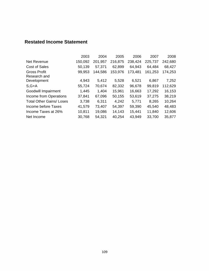
109
Restated Income Statement
2003 2004 2005 2006 2007 2008Net Revenue 150,092 201,957 216,875 238,424 225,737 242,680Cost of Sales 50,139 57,371 62,899 64,943 64,484 68,427Gross Profit 99,953 144,586 153,976 173,481 161,253 174,253Research and Development 4,943 5,412 5,528 6,521 6,867 7,252S,G+A 55,724 70,674 82,332 96,678 99,819 112,629Goodwill Impairment 1,445 1,404 15,961 16,663 17,292 16,153Income from Operations 37,841 67,096 50,155 53,619 37,275 38,219Total Other Gains/ Loses 3,738 6,311 4,242 5,771 8,265 10,264Income before Taxes 41,579 73,407 54,397 59,390 45,540 48,483Income Taxes at 26% 10,811 19,086 14,143 15,441 11,840 12,606Net Income 30,768 54,321 40,254 43,949 33,700 35,877
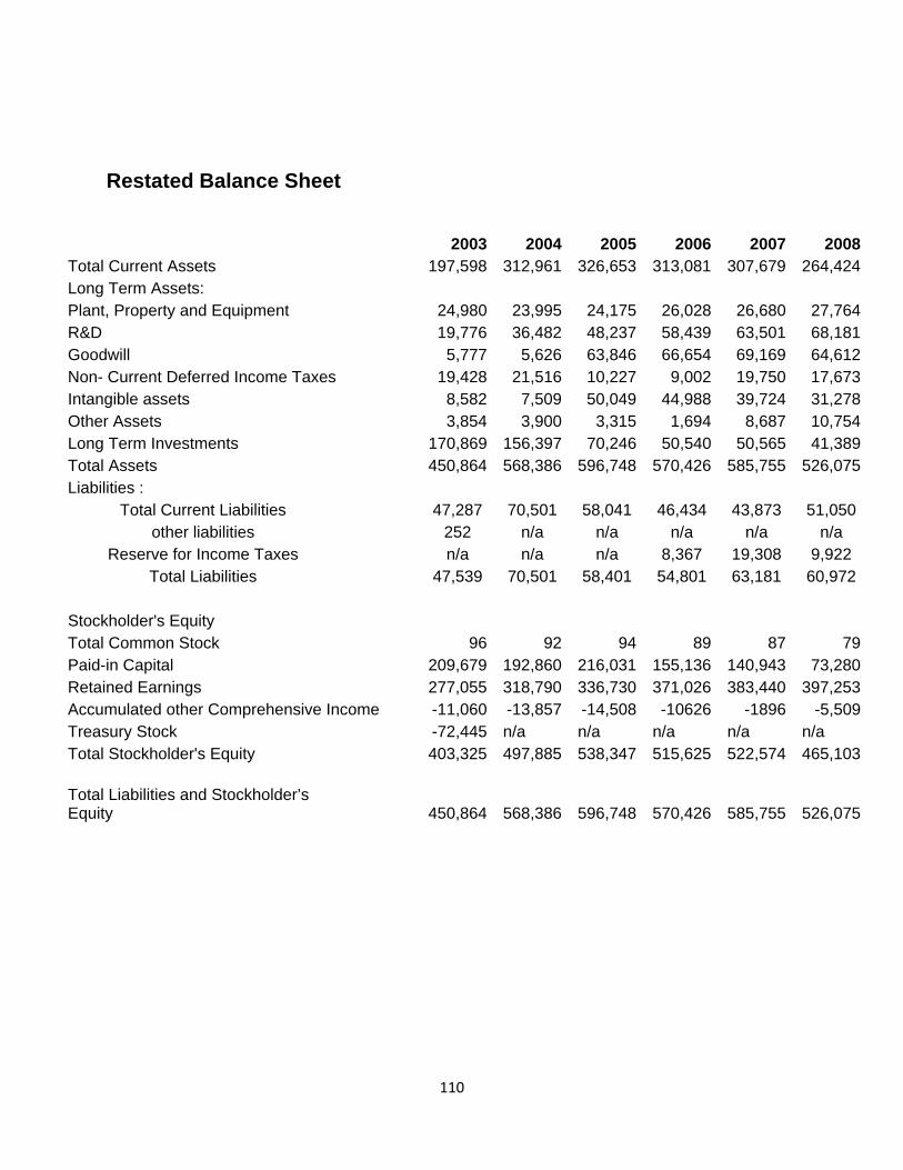
110
Restated Balance Sheet
2003 2004 2005 2006 2007 2008Total Current Assets 197,598 312,961 326,653 313,081 307,679 264,424Long Term Assets: Plant, Property and Equipment 24,980 23,995 24,175 26,028 26,680 27,764R&D 19,776 36,482 48,237 58,439 63,501 68,181Goodwill 5,777 5,626 63,846 66,654 69,169 64,612Non- Current Deferred Income Taxes 19,428 21,516 10,227 9,002 19,750 17,673Intangible assets 8,582 7,509 50,049 44,988 39,724 31,278Other Assets 3,854 3,900 3,315 1,694 8,687 10,754Long Term Investments 170,869 156,397 70,246 50,540 50,565 41,389Total Assets 450,864 568,386 596,748 570,426 585,755 526,075Liabilities :
Total Current Liabilities 47,287 70,501 58,041 46,434 43,873 51,050 other liabilities 252 n/a n/a n/a n/a n/a
Reserve for Income Taxes n/a n/a n/a 8,367 19,308 9,922 Total Liabilities 47,539 70,501 58,401 54,801 63,181 60,972
Stockholder's Equity Total Common Stock 96 92 94 89 87 79Paid-in Capital 209,679 192,860 216,031 155,136 140,943 73,280Retained Earnings 277,055 318,790 336,730 371,026 383,440 397,253Accumulated other Comprehensive Income -11,060 -13,857 -14,508 -10626 -1896 -5,509Treasury Stock -72,445 n/a n/a n/a n/a n/a Total Stockholder's Equity 403,325 497,885 538,347 515,625 522,574 465,103
Total Liabilities and Stockholder’s Equity 450,864 568,386 596,748 570,426 585,755 526,075
111
Financial Analysis, Forecasting financials, and Cost of Capital Estimation
In order to continue in thoroughly evaluating a firm, an analyst must first complete ratio analysis,
then forecast the financial statements, and establish the cost of capital for the firm. Calculations of
ratios such as liquidity ratios, profitability ratios, and capital structure ratios; allows an analyst to
compare trends across the firms in an industry giving them a clearer picture of how each firm stacks up
against its competitors. After the completion of the ratio analysis; using past data, we will be able to
forecast the income statement, the balance sheet, and the statement of cash flows for Cognex over the
next several years. Once the forecasting is finalized we will be able to calculate the firms cost of
capital, which will ultimately aide us in our final valuation of the firm.
Financial Analysis
Comparing financial statements of the firms within an industry illustrates the capital structure,
liquidity, and profitability of those firms against one another. The use of ratios allows analysts to draw
more accurate conclusions of how each company performs relative to others in its sector with regard to
uniform calculations. The use of financial analysis ratios provides less complexity in the comparison
process. The ratios derived in the financial analysis section are then used to determining the proper
forecasts for the firm.
112
Liquidity ratio Analysis
The use of liquidity ratios allows investors and analysts to achieve a better understanding of
how quickly a firm can pay off its short term debt obligations. Liquidity ratios show the firm’s ability to
pay current debts as they become due. These ratios can be used to explain the basic health within a
firm. Overall, higher ratios indicate more financial safety within a firm. Liquidity ratios include; the
current ratio, quick asset ratio, accounts receivable turnover, days’ supply of receivables, inventory
turnover, days’ supply of inventory, and working capital turnover. Analyzing and comparing these ratios
will give an investor a clearer understanding of how liquid a particular firm is with respect to its industry.
Current Ratio:
The current ratio can be calculated by dividing a firm’s current assets by its current liabilities.
This ratio explains the amount of financial coverage a firm has at any given time. It tells an analyst
how well a company can meet its current debt obligations based on the amount of current assets the
firm holds. A ratio below one would indicate that a firm has more current debt obligations due than it
has current assets to cover those debts. This would signify a high liquidity risk within the firm. A ratio
above one would show that the firm has a substantial amount of current assets to meet the amount of
current obligations due. Cognex maintains a ratio higher than most companies in the industry.
However, after calculating the ratio with restated numbers Cognex appears more average with the
industry. Cognex saw an increase in their current ratio between 2003 and 2006, and a slight decrease
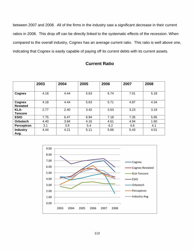
113
between 2007 and 2008. All of the firms in the industry saw a significant decrease in their current
ratios in 2008. This drop off can be directly linked to the systematic effects of the recession. When
compared to the overall industry, Cognex has an average current ratio. This ratio is well above one,
indicating that Cognex is easily capable of paying off its current debts with its current assets.
Current Ratio
2003 2004 2005 2006 2007 2008
Cognex 4.18 4.44 5.63 6.74 7.01 5.18
Cognex Restated
4.18 4.44 5.63 5.71 4.87 4.34
KLA-Tencore
2.77 2.40 3.42 3.53 3.23 3.19
ESIO 7.75 6.47 6.94 7.18 7.35 5.95 Orbotech 4.40 3.84 4.16 4.61 4.94 1.60 Perceptron 3.1 3.9 5.4 6.2 4.6 4.1 Industry Avg.
4.44 4.21 5.11 5.66 5.43 4.01
0.00
1.00
2.00
3.00
4.00
5.00
6.00
7.00
8.00
9.00
2003 2004 2005 2006 2007 2008
Cognex
Cognex Restated
KLA‐Tencore
ESIO
Orbotech
Perceptron
Industry Avg.
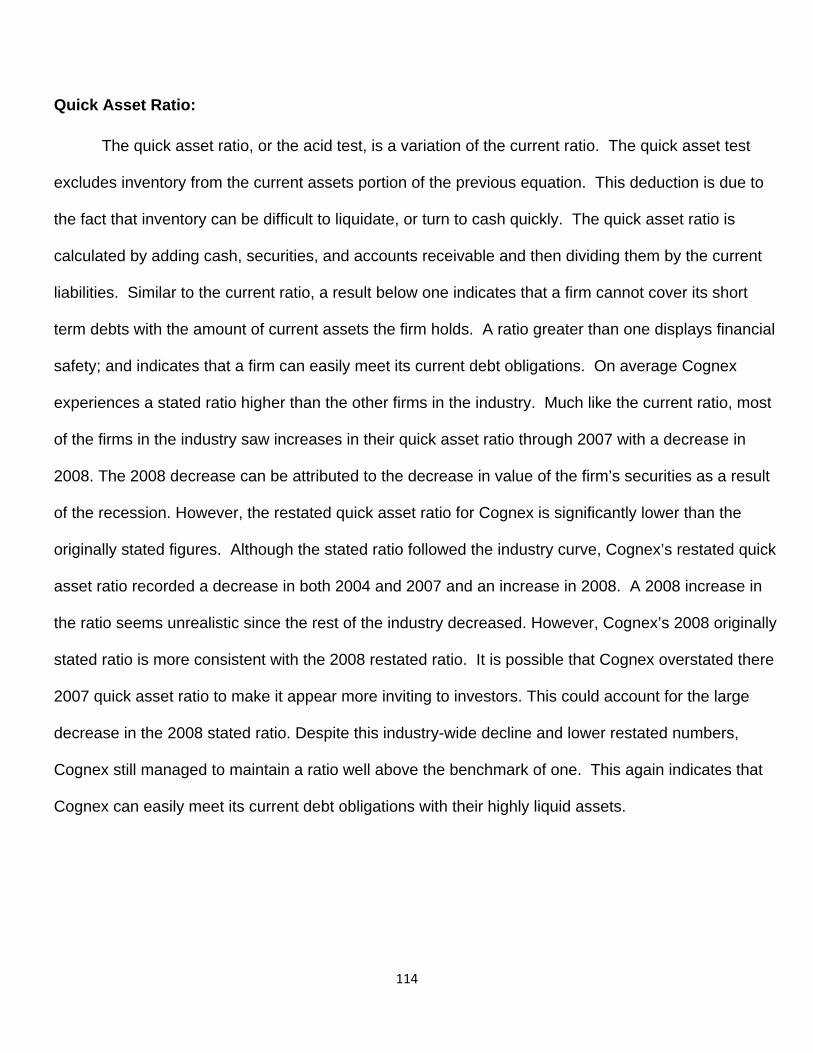
114
Quick Asset Ratio:
The quick asset ratio, or the acid test, is a variation of the current ratio. The quick asset test
excludes inventory from the current assets portion of the previous equation. This deduction is due to
the fact that inventory can be difficult to liquidate, or turn to cash quickly. The quick asset ratio is
calculated by adding cash, securities, and accounts receivable and then dividing them by the current
liabilities. Similar to the current ratio, a result below one indicates that a firm cannot cover its short
term debts with the amount of current assets the firm holds. A ratio greater than one displays financial
safety; and indicates that a firm can easily meet its current debt obligations. On average Cognex
experiences a stated ratio higher than the other firms in the industry. Much like the current ratio, most
of the firms in the industry saw increases in their quick asset ratio through 2007 with a decrease in
2008. The 2008 decrease can be attributed to the decrease in value of the firm’s securities as a result
of the recession. However, the restated quick asset ratio for Cognex is significantly lower than the
originally stated figures. Although the stated ratio followed the industry curve, Cognex’s restated quick
asset ratio recorded a decrease in both 2004 and 2007 and an increase in 2008. A 2008 increase in
the ratio seems unrealistic since the rest of the industry decreased. However, Cognex’s 2008 originally
stated ratio is more consistent with the 2008 restated ratio. It is possible that Cognex overstated there
2007 quick asset ratio to make it appear more inviting to investors. This could account for the large
decrease in the 2008 stated ratio. Despite this industry-wide decline and lower restated numbers,
Cognex still managed to maintain a ratio well above the benchmark of one. This again indicates that
Cognex can easily meet its current debt obligations with their highly liquid assets.
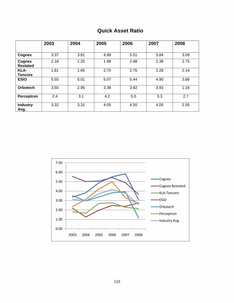
115
Quick Asset Ratio
2003 2004 2005 2006 2007 2008
Cognex 3.37 3.81 4.89 5.51 5.84 3.09
Cognex Restated
2.18 1.25 1.98 2.48 2.38 2.75
KLA-Tencore
1.81 1.65 2.70 2.76 2.28 2.14
ESIO 5.55 5.01 5.07 5.44 4.90 3.66
Orbotech 3.50 2.95 3.38 3.82 3.93 1.16
Perceptron 2.4 3.1 4.2 5.0 3.3 2.7
Industry Avg.
3.32 3.31 4.05 4.50 4.05 2.55
0.00
1.00
2.00
3.00
4.00
5.00
6.00
7.00
2003 2004 2005 2006 2007 2008
Cognex
Cognex Restated
KLA‐Tencore
ESIO
Orbotech
Perceptron
Industry Avg.
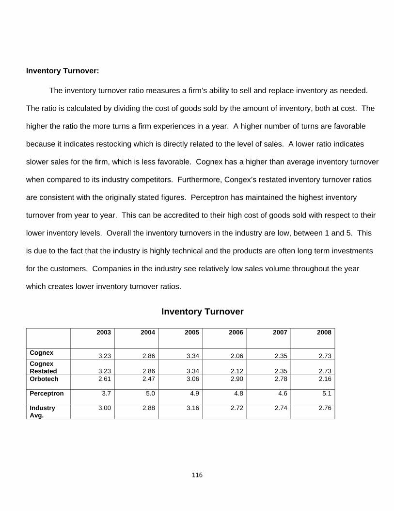
116
Inventory Turnover:
The inventory turnover ratio measures a firm’s ability to sell and replace inventory as needed.
The ratio is calculated by dividing the cost of goods sold by the amount of inventory, both at cost. The
higher the ratio the more turns a firm experiences in a year. A higher number of turns are favorable
because it indicates restocking which is directly related to the level of sales. A lower ratio indicates
slower sales for the firm, which is less favorable. Cognex has a higher than average inventory turnover
when compared to its industry competitors. Furthermore, Congex’s restated inventory turnover ratios
are consistent with the originally stated figures. Perceptron has maintained the highest inventory
turnover from year to year. This can be accredited to their high cost of goods sold with respect to their
lower inventory levels. Overall the inventory turnovers in the industry are low, between 1 and 5. This
is due to the fact that the industry is highly technical and the products are often long term investments
for the customers. Companies in the industry see relatively low sales volume throughout the year
which creates lower inventory turnover ratios.
Inventory Turnover
2003 2004 2005 2006 2007 2008
Cognex 3.23 2.86 3.34 2.06 2.35 2.73Cognex Restated 3.23 2.86 3.34 2.12 2.35 2.73Orbotech 2.61 2.47 3.06 2.90 2.78 2.16
Perceptron 3.7 5.0 4.9 4.8 4.6 5.1
Industry Avg.
3.00 2.88 3.16 2.72 2.74 2.76
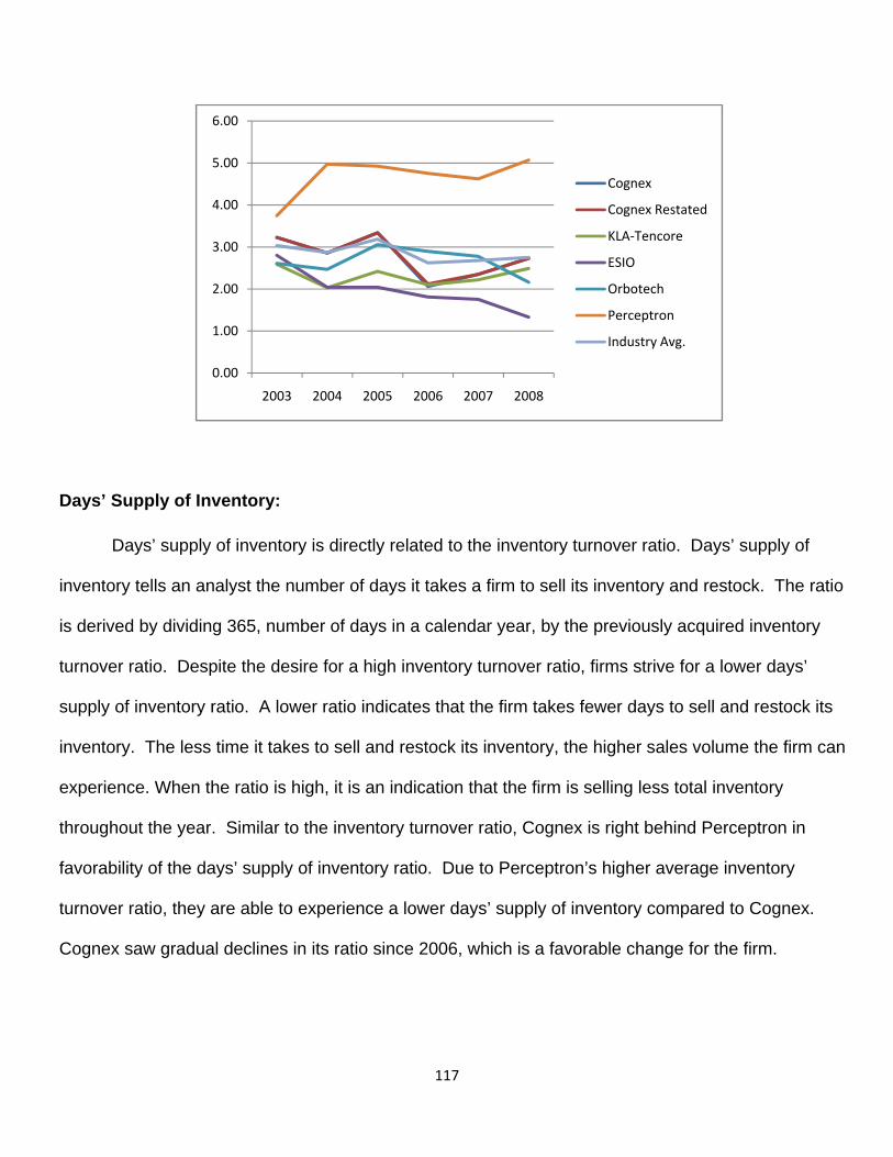
117
Days’ Supply of Inventory:
Days’ supply of inventory is directly related to the inventory turnover ratio. Days’ supply of
inventory tells an analyst the number of days it takes a firm to sell its inventory and restock. The ratio
is derived by dividing 365, number of days in a calendar year, by the previously acquired inventory
turnover ratio. Despite the desire for a high inventory turnover ratio, firms strive for a lower days’
supply of inventory ratio. A lower ratio indicates that the firm takes fewer days to sell and restock its
inventory. The less time it takes to sell and restock its inventory, the higher sales volume the firm can
experience. When the ratio is high, it is an indication that the firm is selling less total inventory
throughout the year. Similar to the inventory turnover ratio, Cognex is right behind Perceptron in
favorability of the days’ supply of inventory ratio. Due to Perceptron’s higher average inventory
turnover ratio, they are able to experience a lower days’ supply of inventory compared to Cognex.
Cognex saw gradual declines in its ratio since 2006, which is a favorable change for the firm.
0.00
1.00
2.00
3.00
4.00
5.00
6.00
2003 2004 2005 2006 2007 2008
Cognex
Cognex Restated
KLA‐Tencore
ESIO
Orbotech
Perceptron
Industry Avg.
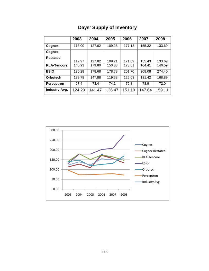
118
Days’ Supply of Inventory
2003 2004 2005 2006 2007 2008 Cognex 113.00 127.62 109.28 177.18 155.32 133.69
Cognex Restated
112.97 127.82 109.21 171.89 155.43 133.69 KLA-Tencore 140.93 179.80 150.83 173.81 164.41 146.59
ESIO 130.28 178.68 178.78 201.70 208.08 274.40
Orbotech 139.78 147.88 119.38 126.03 131.42 168.89
Perceptron 97.4 73.4 74.1 76.8 78.9 72.0
Industry Avg. 124.29 141.47 126.47 151.10 147.64 159.11
0.00
50.00
100.00
150.00
200.00
250.00
300.00
2003 2004 2005 2006 2007 2008
Cognex
Cognex Restated
KLA‐Tencore
ESIO
Orbotech
Perceptron
Industry Avg.
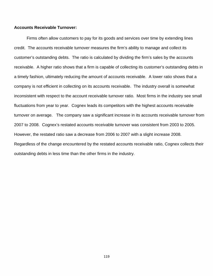
119
Accounts Receivable Turnover:
Firms often allow customers to pay for its goods and services over time by extending lines
credit. The accounts receivable turnover measures the firm’s ability to manage and collect its
customer’s outstanding debts. The ratio is calculated by dividing the firm’s sales by the accounts
receivable. A higher ratio shows that a firm is capable of collecting its customer’s outstanding debts in
a timely fashion, ultimately reducing the amount of accounts receivable. A lower ratio shows that a
company is not efficient in collecting on its accounts receivable. The industry overall is somewhat
inconsistent with respect to the account receivable turnover ratio. Most firms in the industry see small
fluctuations from year to year. Cognex leads its competitors with the highest accounts receivable
turnover on average. The company saw a significant increase in its accounts receivable turnover from
2007 to 2008. Cognex’s restated accounts receivable turnover was consistent from 2003 to 2005.
However, the restated ratio saw a decrease from 2006 to 2007 with a slight increase 2008.
Regardless of the change encountered by the restated accounts receivable ratio, Cognex collects their
outstanding debts in less time than the other firms in the industry.
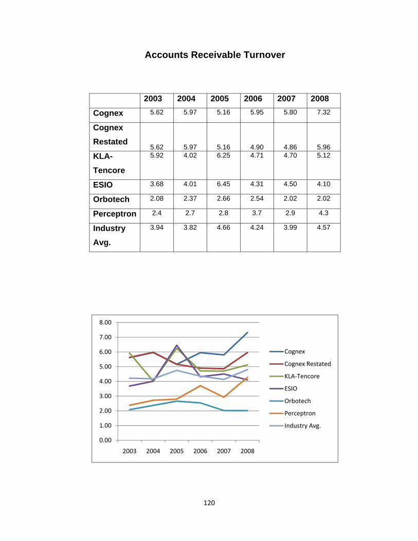
120
Accounts Receivable Turnover
2003 2004 2005 2006 2007 2008
Cognex 5.62 5.97 5.16 5.95 5.80 7.32
Cognex Restated
5.62 5.97 5.16 4.90 4.86 5.96 KLA-Tencore
5.92 4.02 6.25 4.71 4.70 5.12
ESIO 3.68 4.01 6.45 4.31 4.50 4.10
Orbotech 2.08 2.37 2.66 2.54 2.02 2.02
Perceptron 2.4 2.7 2.8 3.7 2.9 4.3
Industry Avg.
3.94 3.82 4.66 4.24 3.99 4.57
0.00
1.00
2.00
3.00
4.00
5.00
6.00
7.00
8.00
2003 2004 2005 2006 2007 2008
Cognex
Cognex Restated
KLA‐Tencore
ESIO
Orbotech
Perceptron
Industry Avg.
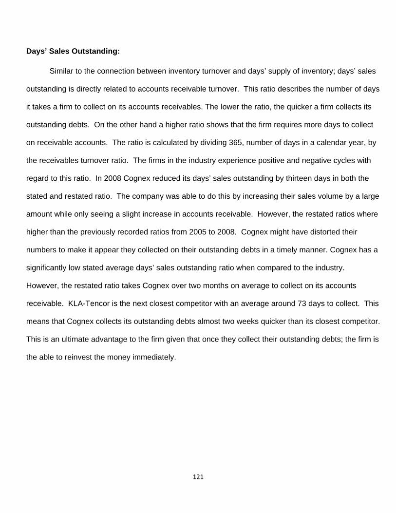
121
Days’ Sales Outstanding:
Similar to the connection between inventory turnover and days’ supply of inventory; days’ sales
outstanding is directly related to accounts receivable turnover. This ratio describes the number of days
it takes a firm to collect on its accounts receivables. The lower the ratio, the quicker a firm collects its
outstanding debts. On the other hand a higher ratio shows that the firm requires more days to collect
on receivable accounts. The ratio is calculated by dividing 365, number of days in a calendar year, by
the receivables turnover ratio. The firms in the industry experience positive and negative cycles with
regard to this ratio. In 2008 Cognex reduced its days’ sales outstanding by thirteen days in both the
stated and restated ratio. The company was able to do this by increasing their sales volume by a large
amount while only seeing a slight increase in accounts receivable. However, the restated ratios where
higher than the previously recorded ratios from 2005 to 2008. Cognex might have distorted their
numbers to make it appear they collected on their outstanding debts in a timely manner. Cognex has a
significantly low stated average days’ sales outstanding ratio when compared to the industry.
However, the restated ratio takes Cognex over two months on average to collect on its accounts
receivable. KLA-Tencor is the next closest competitor with an average around 73 days to collect. This
means that Cognex collects its outstanding debts almost two weeks quicker than its closest competitor.
This is an ultimate advantage to the firm given that once they collect their outstanding debts; the firm is
the able to reinvest the money immediately.
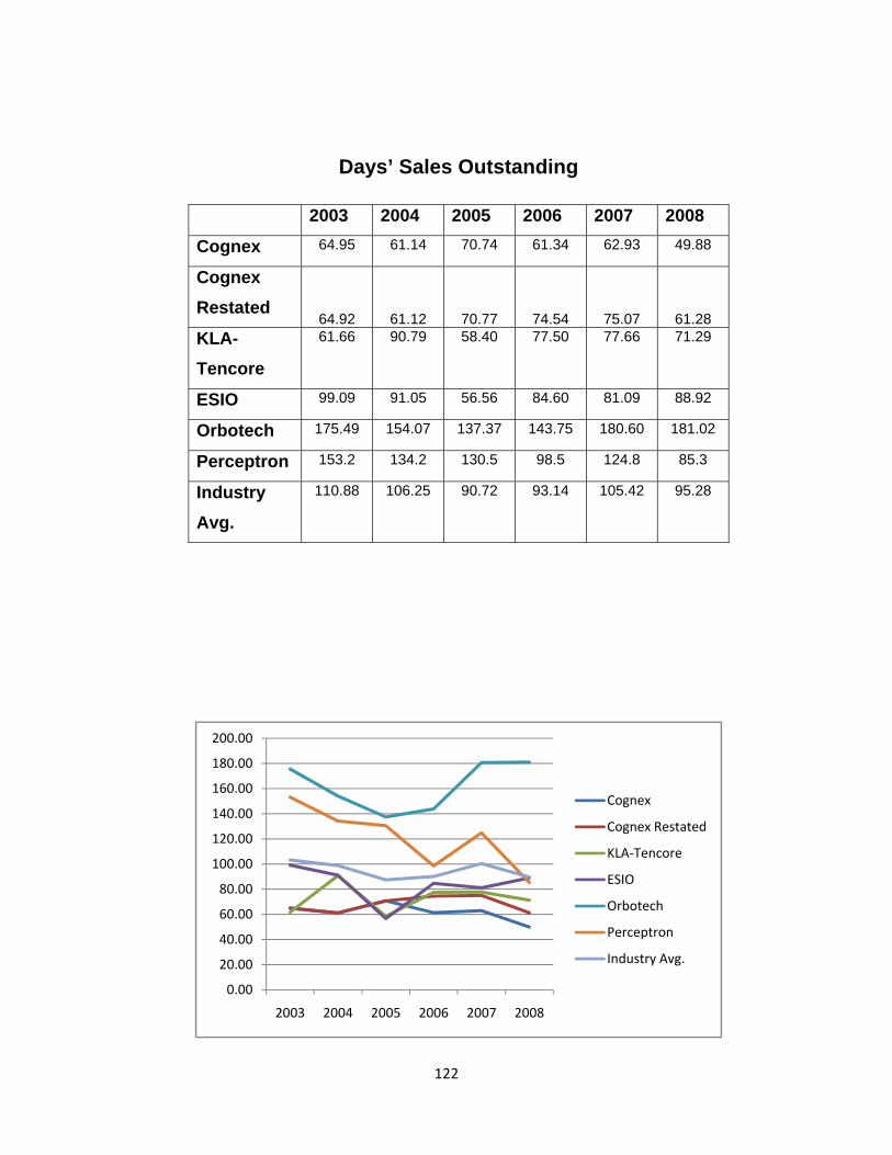
122
Days’ Sales Outstanding
2003 2004 2005 2006 2007 2008
Cognex 64.95 61.14 70.74 61.34 62.93 49.88
Cognex Restated
64.92 61.12 70.77 74.54 75.07 61.28 KLA-Tencore
61.66 90.79 58.40 77.50 77.66 71.29
ESIO 99.09 91.05 56.56 84.60 81.09 88.92
Orbotech 175.49 154.07 137.37 143.75 180.60 181.02
Perceptron 153.2 134.2 130.5 98.5 124.8 85.3
Industry Avg.
110.88 106.25 90.72 93.14 105.42 95.28
0.00
20.00
40.00
60.00
80.00
100.00
120.00
140.00
160.00
180.00
200.00
2003 2004 2005 2006 2007 2008
Cognex
Cognex Restated
KLA‐Tencore
ESIO
Orbotech
Perceptron
Industry Avg.
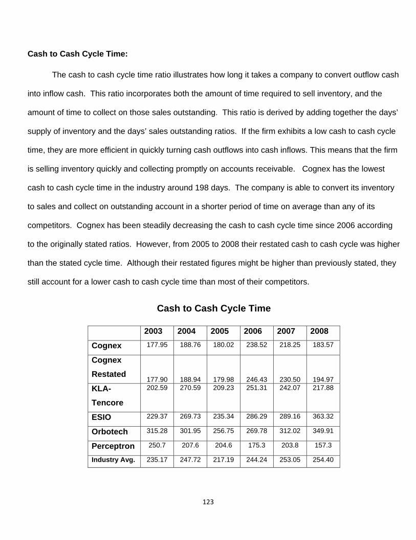
123
Cash to Cash Cycle Time:
The cash to cash cycle time ratio illustrates how long it takes a company to convert outflow cash
into inflow cash. This ratio incorporates both the amount of time required to sell inventory, and the
amount of time to collect on those sales outstanding. This ratio is derived by adding together the days’
supply of inventory and the days’ sales outstanding ratios. If the firm exhibits a low cash to cash cycle
time, they are more efficient in quickly turning cash outflows into cash inflows. This means that the firm
is selling inventory quickly and collecting promptly on accounts receivable. Cognex has the lowest
cash to cash cycle time in the industry around 198 days. The company is able to convert its inventory
to sales and collect on outstanding account in a shorter period of time on average than any of its
competitors. Cognex has been steadily decreasing the cash to cash cycle time since 2006 according
to the originally stated ratios. However, from 2005 to 2008 their restated cash to cash cycle was higher
than the stated cycle time. Although their restated figures might be higher than previously stated, they
still account for a lower cash to cash cycle time than most of their competitors.
Cash to Cash Cycle Time
2003 2004 2005 2006 2007 2008
Cognex 177.95 188.76 180.02 238.52 218.25 183.57
Cognex Restated
177.90 188.94 179.98 246.43 230.50 194.97 KLA-Tencore
202.59 270.59 209.23 251.31 242.07 217.88
ESIO 229.37 269.73 235.34 286.29 289.16 363.32
Orbotech 315.28 301.95 256.75 269.78 312.02 349.91
Perceptron 250.7 207.6 204.6 175.3 203.8 157.3
Industry Avg. 235.17 247.72 217.19 244.24 253.05 254.40
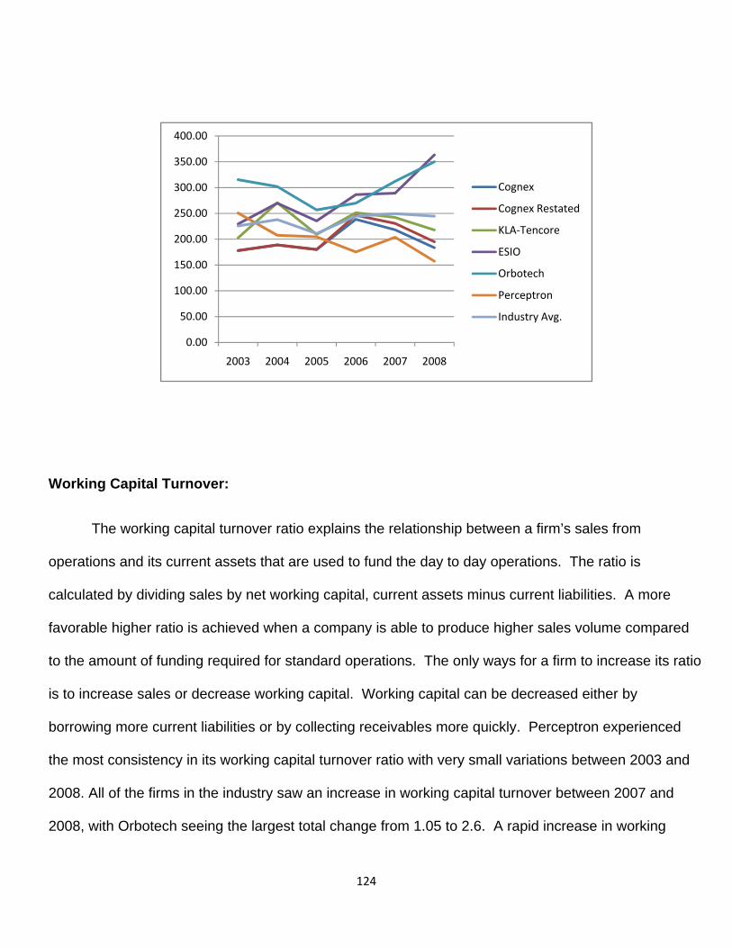
124
Working Capital Turnover:
The working capital turnover ratio explains the relationship between a firm’s sales from
operations and its current assets that are used to fund the day to day operations. The ratio is
calculated by dividing sales by net working capital, current assets minus current liabilities. A more
favorable higher ratio is achieved when a company is able to produce higher sales volume compared
to the amount of funding required for standard operations. The only ways for a firm to increase its ratio
is to increase sales or decrease working capital. Working capital can be decreased either by
borrowing more current liabilities or by collecting receivables more quickly. Perceptron experienced
the most consistency in its working capital turnover ratio with very small variations between 2003 and
2008. All of the firms in the industry saw an increase in working capital turnover between 2007 and
2008, with Orbotech seeing the largest total change from 1.05 to 2.6. A rapid increase in working
0.00
50.00
100.00
150.00
200.00
250.00
300.00
350.00
400.00
2003 2004 2005 2006 2007 2008
Cognex
Cognex Restated
KLA‐Tencore
ESIO
Orbotech
Perceptron
Industry Avg.
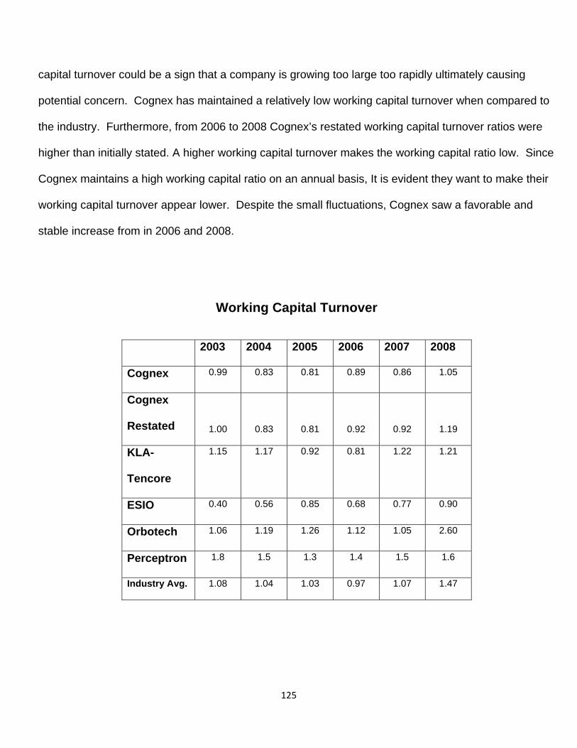
125
capital turnover could be a sign that a company is growing too large too rapidly ultimately causing
potential concern. Cognex has maintained a relatively low working capital turnover when compared to
the industry. Furthermore, from 2006 to 2008 Cognex’s restated working capital turnover ratios were
higher than initially stated. A higher working capital turnover makes the working capital ratio low. Since
Cognex maintains a high working capital ratio on an annual basis, It is evident they want to make their
working capital turnover appear lower. Despite the small fluctuations, Cognex saw a favorable and
stable increase from in 2006 and 2008.
Working Capital Turnover
2003 2004 2005 2006 2007 2008
Cognex 0.99 0.83 0.81 0.89 0.86 1.05
Cognex
Restated 1.00 0.83 0.81 0.92 0.92 1.19
KLA-
Tencore
1.15 1.17 0.92 0.81 1.22 1.21
ESIO 0.40 0.56 0.85 0.68 0.77 0.90
Orbotech 1.06 1.19 1.26 1.12 1.05 2.60
Perceptron 1.8 1.5 1.3 1.4 1.5 1.6
Industry Avg. 1.08 1.04 1.03 0.97 1.07 1.47
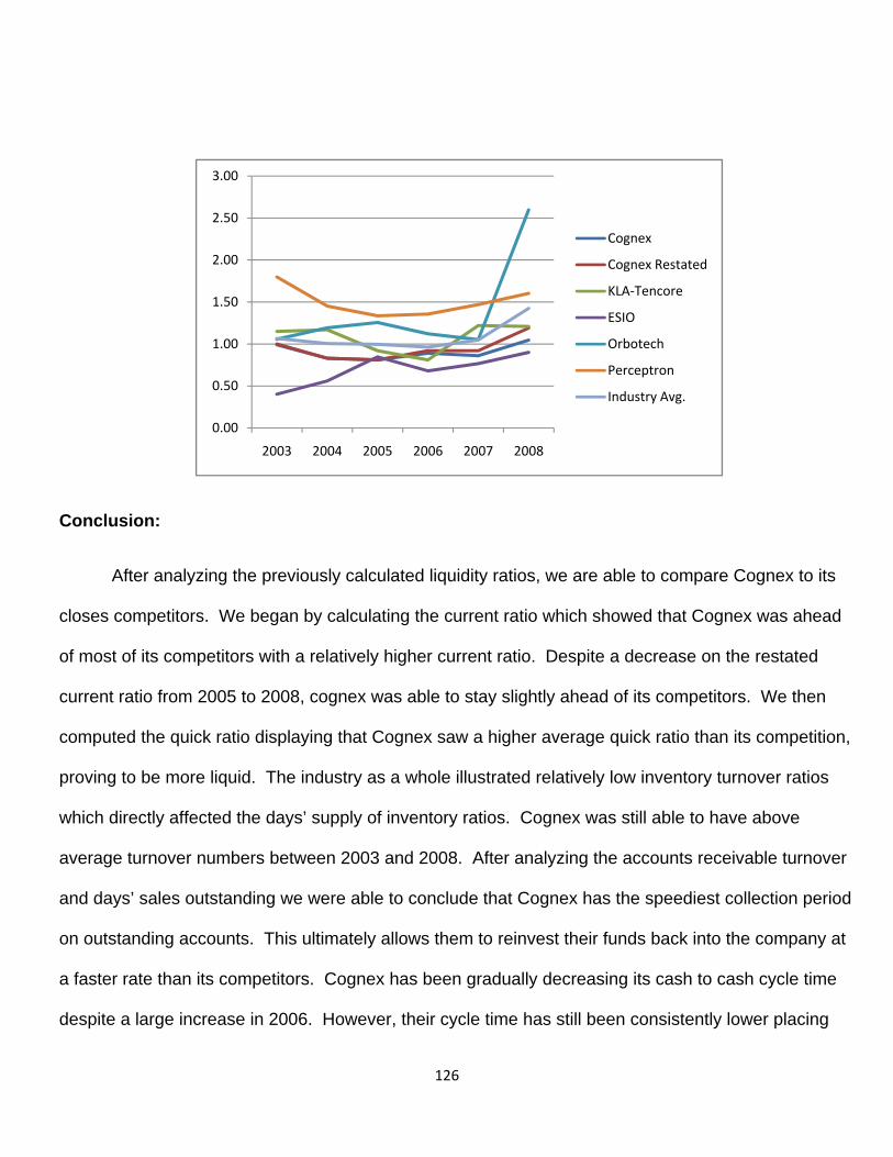
126
Conclusion:
After analyzing the previously calculated liquidity ratios, we are able to compare Cognex to its
closes competitors. We began by calculating the current ratio which showed that Cognex was ahead
of most of its competitors with a relatively higher current ratio. Despite a decrease on the restated
current ratio from 2005 to 2008, cognex was able to stay slightly ahead of its competitors. We then
computed the quick ratio displaying that Cognex saw a higher average quick ratio than its competition,
proving to be more liquid. The industry as a whole illustrated relatively low inventory turnover ratios
which directly affected the days’ supply of inventory ratios. Cognex was still able to have above
average turnover numbers between 2003 and 2008. After analyzing the accounts receivable turnover
and days’ sales outstanding we were able to conclude that Cognex has the speediest collection period
on outstanding accounts. This ultimately allows them to reinvest their funds back into the company at
a faster rate than its competitors. Cognex has been gradually decreasing its cash to cash cycle time
despite a large increase in 2006. However, their cycle time has still been consistently lower placing
0.00
0.50
1.00
1.50
2.00
2.50
3.00
2003 2004 2005 2006 2007 2008
Cognex
Cognex Restated
KLA‐Tencore
ESIO
Orbotech
Perceptron
Industry Avg.
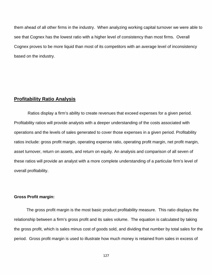
127
them ahead of all other firms in the industry. When analyzing working capital turnover we were able to
see that Cognex has the lowest ratio with a higher level of consistency than most firms. Overall
Cognex proves to be more liquid than most of its competitors with an average level of inconsistency
based on the industry.
Profitability Ratio Analysis
Ratios display a firm’s ability to create revenues that exceed expenses for a given period.
Profitability ratios will provide analysts with a deeper understanding of the costs associated with
operations and the levels of sales generated to cover those expenses in a given period. Profitability
ratios include: gross profit margin, operating expense ratio, operating profit margin, net profit margin,
asset turnover, return on assets, and return on equity. An analysis and comparison of all seven of
these ratios will provide an analyst with a more complete understanding of a particular firm’s level of
overall profitability.
Gross Profit margin:
The gross profit margin is the most basic product profitability measure. This ratio displays the
relationship between a firm’s gross profit and its sales volume. The equation is calculated by taking
the gross profit, which is sales minus cost of goods sold, and dividing that number by total sales for the
period. Gross profit margin is used to illustrate how much money is retained from sales in excess of
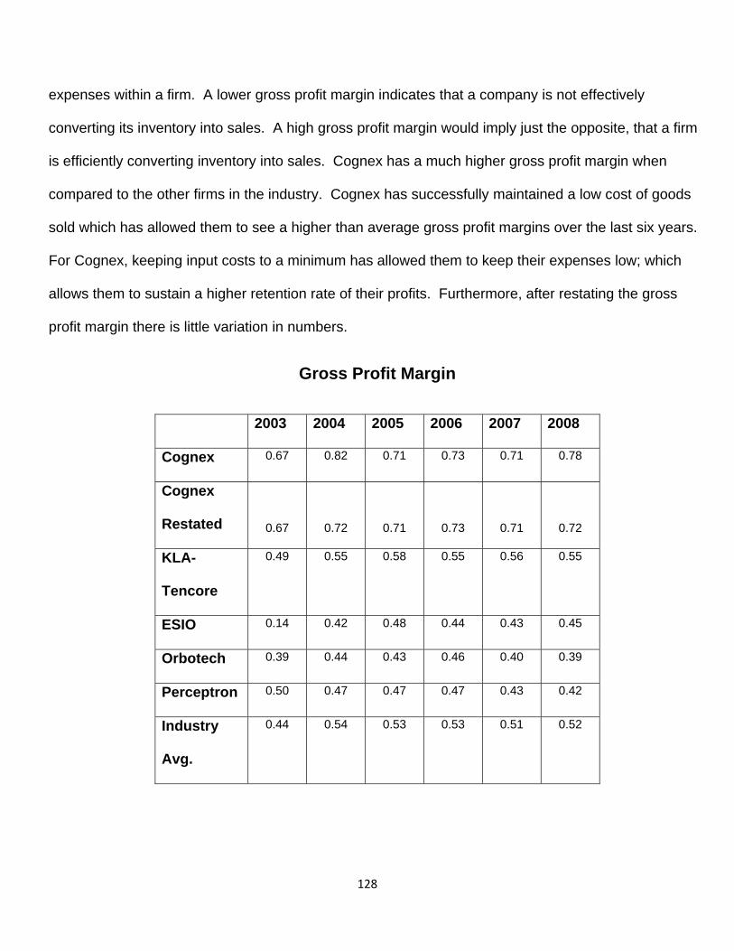
128
expenses within a firm. A lower gross profit margin indicates that a company is not effectively
converting its inventory into sales. A high gross profit margin would imply just the opposite, that a firm
is efficiently converting inventory into sales. Cognex has a much higher gross profit margin when
compared to the other firms in the industry. Cognex has successfully maintained a low cost of goods
sold which has allowed them to see a higher than average gross profit margins over the last six years.
For Cognex, keeping input costs to a minimum has allowed them to keep their expenses low; which
allows them to sustain a higher retention rate of their profits. Furthermore, after restating the gross
profit margin there is little variation in numbers.
Gross Profit Margin
2003 2004 2005 2006 2007 2008
Cognex 0.67 0.82 0.71 0.73 0.71 0.78
Cognex
Restated 0.67 0.72 0.71 0.73 0.71 0.72
KLA-
Tencore
0.49 0.55 0.58 0.55 0.56 0.55
ESIO 0.14 0.42 0.48 0.44 0.43 0.45
Orbotech 0.39 0.44 0.43 0.46 0.40 0.39
Perceptron 0.50 0.47 0.47 0.47 0.43 0.42
Industry
Avg.
0.44 0.54 0.53 0.53 0.51 0.52
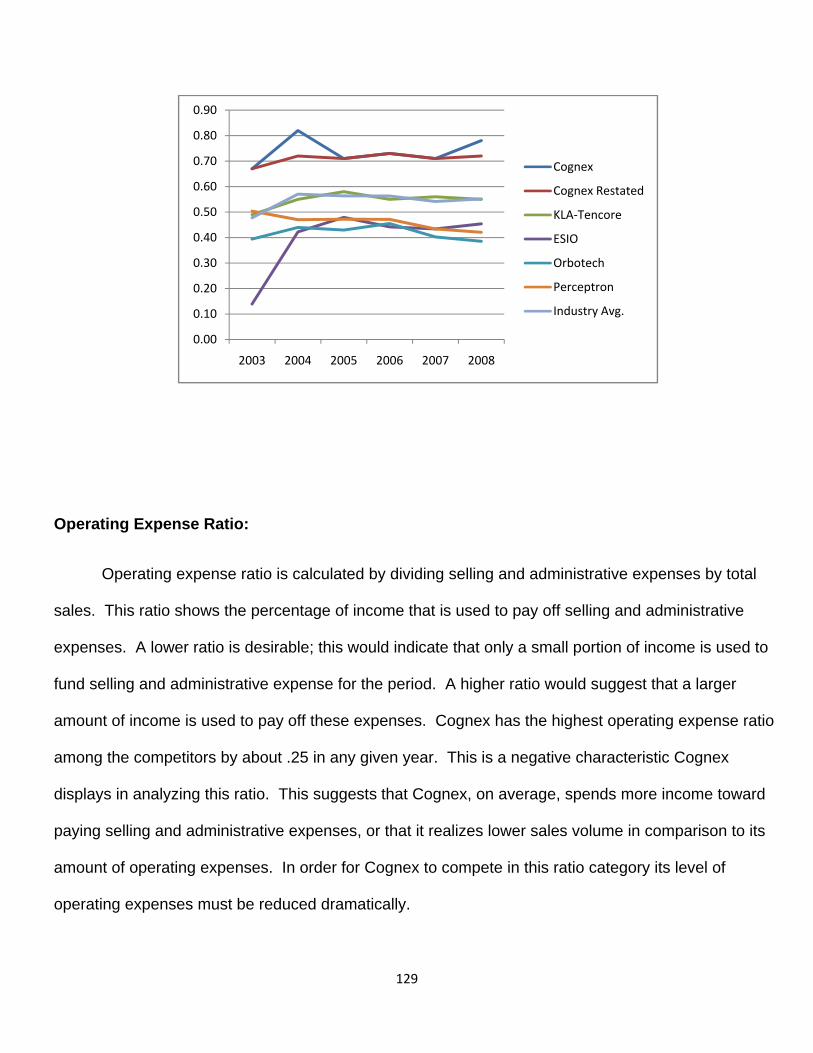
129
Operating Expense Ratio:
Operating expense ratio is calculated by dividing selling and administrative expenses by total
sales. This ratio shows the percentage of income that is used to pay off selling and administrative
expenses. A lower ratio is desirable; this would indicate that only a small portion of income is used to
fund selling and administrative expense for the period. A higher ratio would suggest that a larger
amount of income is used to pay off these expenses. Cognex has the highest operating expense ratio
among the competitors by about .25 in any given year. This is a negative characteristic Cognex
displays in analyzing this ratio. This suggests that Cognex, on average, spends more income toward
paying selling and administrative expenses, or that it realizes lower sales volume in comparison to its
amount of operating expenses. In order for Cognex to compete in this ratio category its level of
operating expenses must be reduced dramatically.
0.00
0.10
0.20
0.30
0.40
0.50
0.60
0.70
0.80
0.90
2003 2004 2005 2006 2007 2008
Cognex
Cognex Restated
KLA‐Tencore
ESIO
Orbotech
Perceptron
Industry Avg.
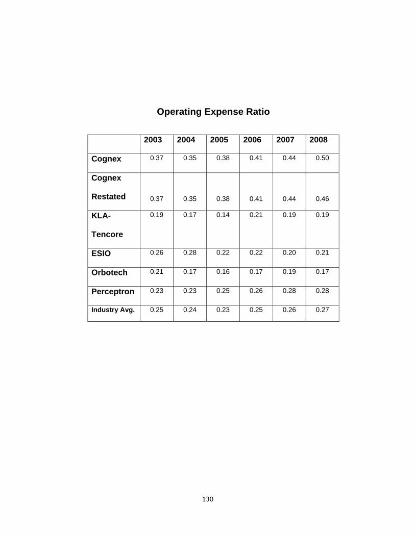
130
Operating Expense Ratio
2003 2004 2005 2006 2007 2008
Cognex 0.37 0.35 0.38 0.41 0.44 0.50
Cognex
Restated 0.37 0.35 0.38 0.41 0.44 0.46
KLA-
Tencore
0.19 0.17 0.14 0.21 0.19 0.19
ESIO 0.26 0.28 0.22 0.22 0.20 0.21
Orbotech 0.21 0.17 0.16 0.17 0.19 0.17
Perceptron 0.23 0.23 0.25 0.26 0.28 0.28
Industry Avg. 0.25 0.24 0.23 0.25 0.26 0.27
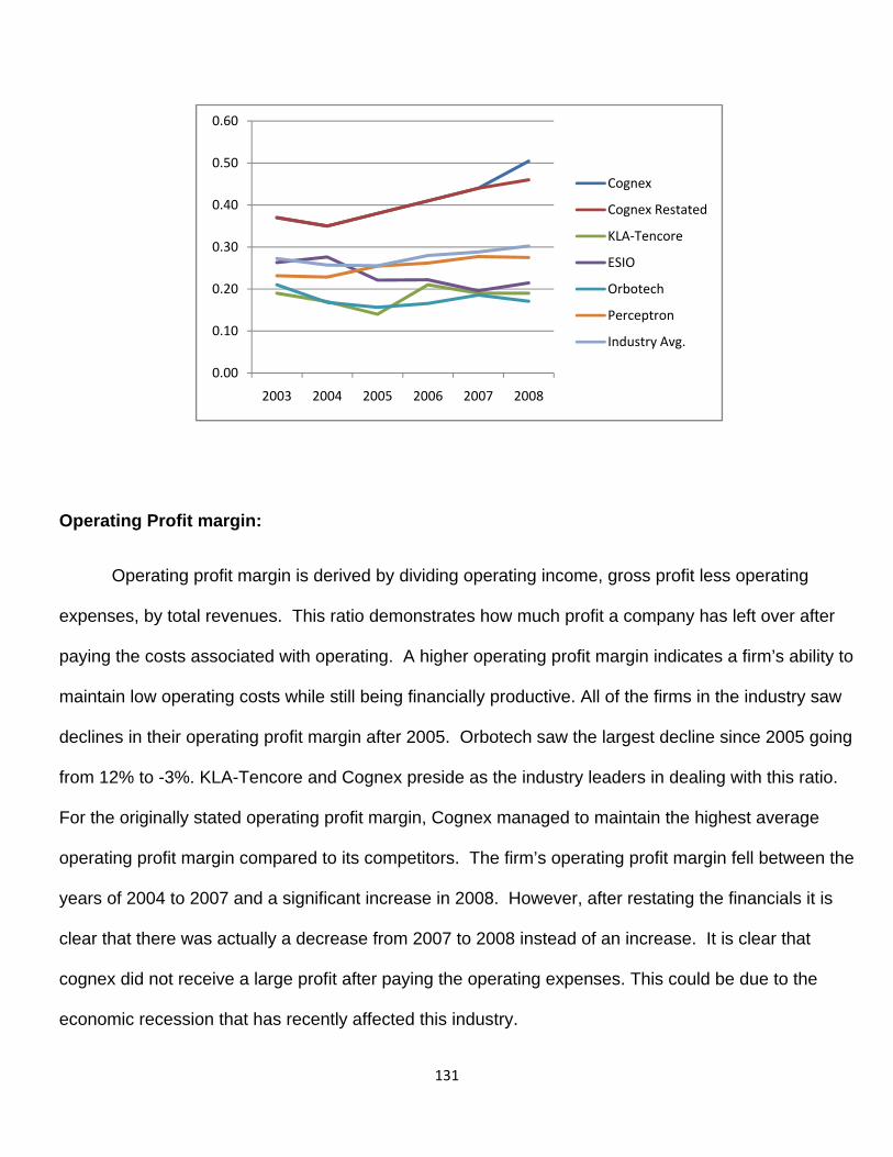
131
Operating Profit margin:
Operating profit margin is derived by dividing operating income, gross profit less operating
expenses, by total revenues. This ratio demonstrates how much profit a company has left over after
paying the costs associated with operating. A higher operating profit margin indicates a firm’s ability to
maintain low operating costs while still being financially productive. All of the firms in the industry saw
declines in their operating profit margin after 2005. Orbotech saw the largest decline since 2005 going
from 12% to -3%. KLA-Tencore and Cognex preside as the industry leaders in dealing with this ratio.
For the originally stated operating profit margin, Cognex managed to maintain the highest average
operating profit margin compared to its competitors. The firm’s operating profit margin fell between the
years of 2004 to 2007 and a significant increase in 2008. However, after restating the financials it is
clear that there was actually a decrease from 2007 to 2008 instead of an increase. It is clear that
cognex did not receive a large profit after paying the operating expenses. This could be due to the
economic recession that has recently affected this industry.
0.00
0.10
0.20
0.30
0.40
0.50
0.60
2003 2004 2005 2006 2007 2008
Cognex
Cognex Restated
KLA‐Tencore
ESIO
Orbotech
Perceptron
Industry Avg.
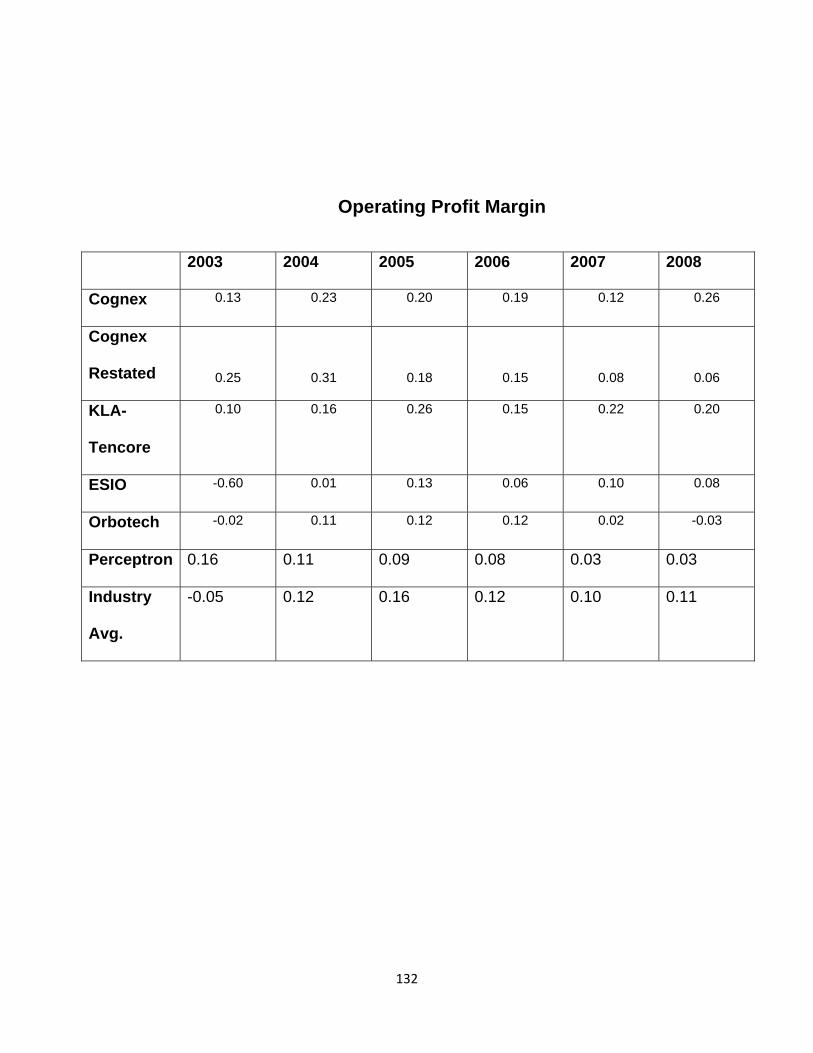
132
Operating Profit Margin
2003 2004 2005 2006 2007 2008
Cognex 0.13 0.23 0.20 0.19 0.12 0.26
Cognex
Restated 0.25 0.31 0.18 0.15 0.08 0.06
KLA-
Tencore
0.10 0.16 0.26 0.15 0.22 0.20
ESIO -0.60 0.01 0.13 0.06 0.10 0.08
Orbotech -0.02 0.11 0.12 0.12 0.02 -0.03
Perceptron 0.16 0.11 0.09 0.08 0.03 0.03
Industry
Avg.
-0.05 0.12 0.16 0.12 0.10 0.11
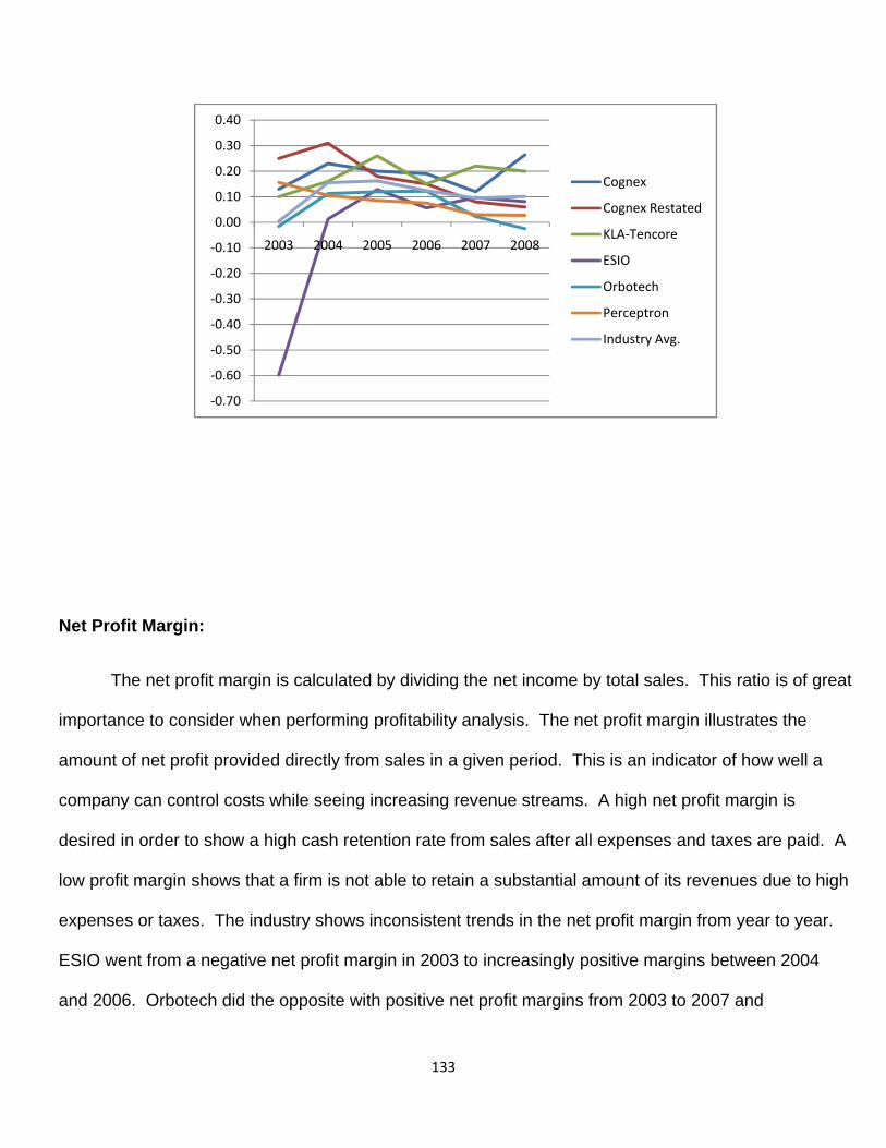
133
Net Profit Margin:
The net profit margin is calculated by dividing the net income by total sales. This ratio is of great
importance to consider when performing profitability analysis. The net profit margin illustrates the
amount of net profit provided directly from sales in a given period. This is an indicator of how well a
company can control costs while seeing increasing revenue streams. A high net profit margin is
desired in order to show a high cash retention rate from sales after all expenses and taxes are paid. A
low profit margin shows that a firm is not able to retain a substantial amount of its revenues due to high
expenses or taxes. The industry shows inconsistent trends in the net profit margin from year to year.
ESIO went from a negative net profit margin in 2003 to increasingly positive margins between 2004
and 2006. Orbotech did the opposite with positive net profit margins from 2003 to 2007 and
‐0.70
‐0.60
‐0.50
‐0.40
‐0.30
‐0.20
‐0.10
0.00
0.10
0.20
0.30
0.40
2003 2004 2005 2006 2007 2008
Cognex
Cognex Restated
KLA‐Tencore
ESIO
Orbotech
Perceptron
Industry Avg.
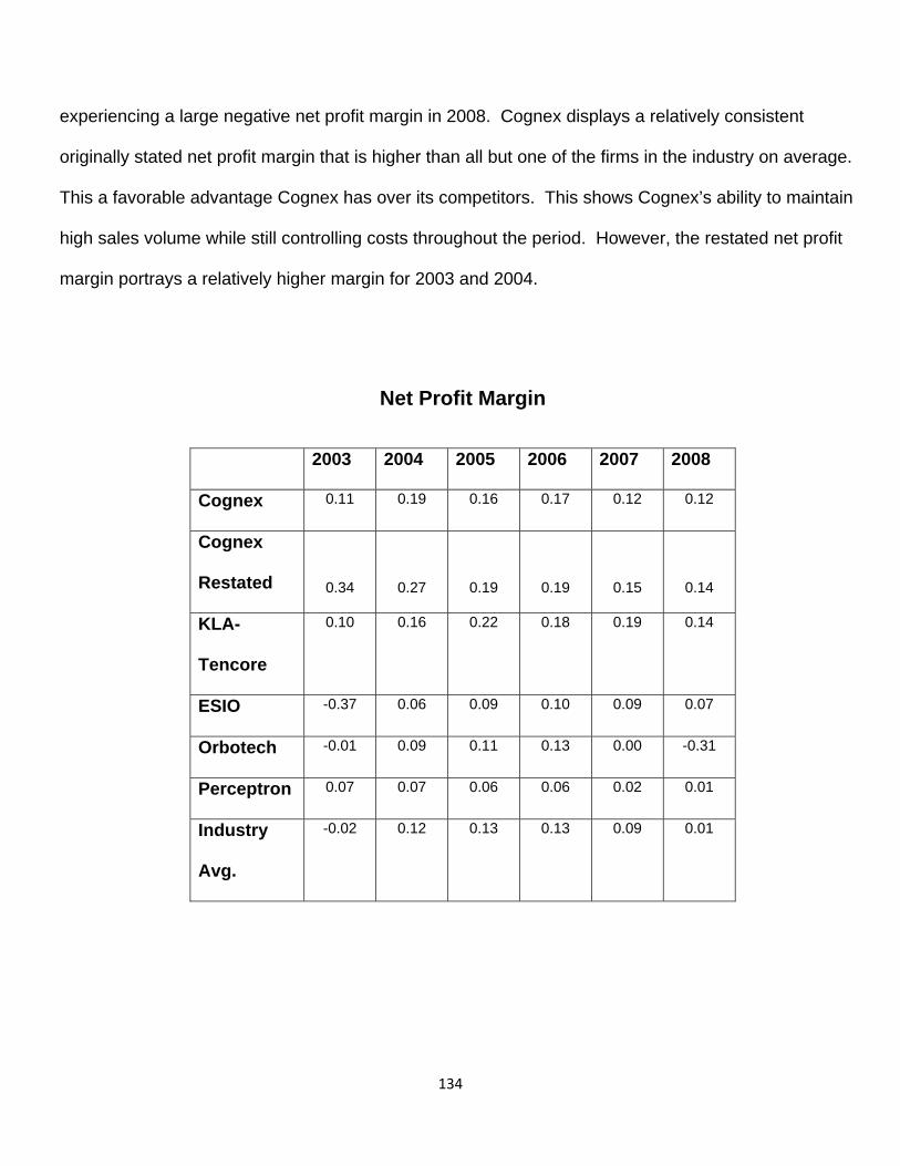
134
experiencing a large negative net profit margin in 2008. Cognex displays a relatively consistent
originally stated net profit margin that is higher than all but one of the firms in the industry on average.
This a favorable advantage Cognex has over its competitors. This shows Cognex’s ability to maintain
high sales volume while still controlling costs throughout the period. However, the restated net profit
margin portrays a relatively higher margin for 2003 and 2004.
Net Profit Margin
2003 2004 2005 2006 2007 2008
Cognex 0.11 0.19 0.16 0.17 0.12 0.12
Cognex
Restated 0.34 0.27 0.19 0.19 0.15 0.14
KLA-
Tencore
0.10 0.16 0.22 0.18 0.19 0.14
ESIO -0.37 0.06 0.09 0.10 0.09 0.07
Orbotech -0.01 0.09 0.11 0.13 0.00 -0.31
Perceptron 0.07 0.07 0.06 0.06 0.02 0.01
Industry
Avg.
-0.02 0.12 0.13 0.13 0.09 0.01
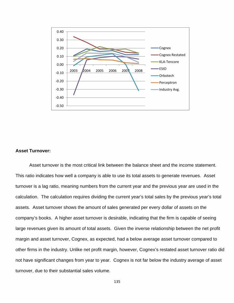
135
Asset Turnover:
Asset turnover is the most critical link between the balance sheet and the income statement.
This ratio indicates how well a company is able to use its total assets to generate revenues. Asset
turnover is a lag ratio, meaning numbers from the current year and the previous year are used in the
calculation. The calculation requires dividing the current year’s total sales by the previous year’s total
assets. Asset turnover shows the amount of sales generated per every dollar of assets on the
company’s books. A higher asset turnover is desirable, indicating that the firm is capable of seeing
large revenues given its amount of total assets. Given the inverse relationship between the net profit
margin and asset turnover, Cognex, as expected, had a below average asset turnover compared to
other firms in the industry. Unlike net profit margin, however, Cognex’s restated asset turnover ratio did
not have significant changes from year to year. Cognex is not far below the industry average of asset
turnover, due to their substantial sales volume.
‐0.50
‐0.40
‐0.30
‐0.20
‐0.10
0.00
0.10
0.20
0.30
0.40
2003 2004 2005 2006 2007 2008
Cognex
Cognex Restated
KLA‐Tencore
ESIO
Orbotech
Perceptron
Industry Avg.
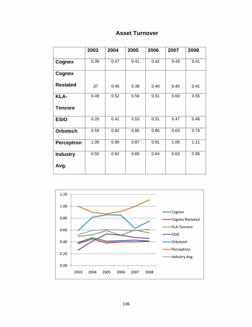
136
Asset Turnover
2003 2004 2005 2006 2007 2008
Cognex 0.39 0.47 0.41 0.42 0.43 0.41
Cognex
Restated .37 0.45 0.38 0.40 0.40 0.41
KLA-
Tencore
0.49 0.52 0.59 0.51 0.60 0.55
ESIO 0.26 0.41 0.53 0.51 0.47 0.46
Orbotech 0.59 0.82 0.86 0.85 0.63 0.75
Perceptron 1.00 0.90 0.87 0.91 1.00 1.11
Industry
Avg.
0.55 0.62 0.65 0.64 0.63 0.66
0.00
0.20
0.40
0.60
0.80
1.00
1.20
2003 2004 2005 2006 2007 2008
Cognex
Cognex Restated
KLA‐Tencore
ESIO
Orbotech
Perceptron
Industry Avg.
137
Return on Asset:
Return on assets (ROA) is a profitability measure that incorporates net profit margin and asset
turnover to indicate how much net income can be generated given the level of assets within a firm.
Return on assets is another lag ratio dealing with numbers from the current year as well as the
previous year. This calculation is derived by dividing the current year’s net income by the previous
year’s total assets. Using the lag ratio allows an analyst to understand how the assets used in the
previous year were able to generate the year end net income. A higher ratio is preferred, indicating
good decision making with regard to asset allocation and cost minimization. A lower ratio would
indicate high costs and an inability to generate net income with assets given. Cognex falls near the
industry average despite seeing a decrease in ROA since 2004. The company saw a greater level of
consistency in ROA as compared to others in the industry. Cognex’s stated and restated return on
assets saw an increase in 2004 and 2005 due to increased net income for the year. However, both
stated and restated ROAs declined slowly from 2006 and 2008. The decline, however, was similar to
the rest of the firms in the industry.
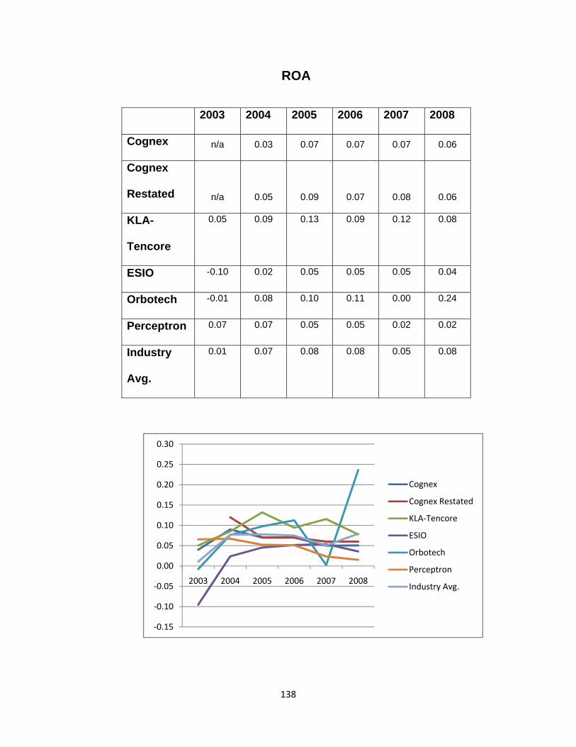
138
ROA
2003 2004 2005 2006 2007 2008
Cognex n/a 0.03 0.07 0.07 0.07 0.06
Cognex
Restated n/a 0.05 0.09 0.07 0.08 0.06
KLA-
Tencore
0.05 0.09 0.13 0.09 0.12 0.08
ESIO -0.10 0.02 0.05 0.05 0.05 0.04
Orbotech -0.01 0.08 0.10 0.11 0.00 0.24
Perceptron 0.07 0.07 0.05 0.05 0.02 0.02
Industry
Avg.
0.01 0.07 0.08 0.08 0.05 0.08
‐0.15
‐0.10
‐0.05
0.00
0.05
0.10
0.15
0.20
0.25
0.30
2003 2004 2005 2006 2007 2008
Cognex
Cognex Restated
KLA‐Tencore
ESIO
Orbotech
Perceptron
Industry Avg.
139
Return on Equity
Return on equity is a ratio that measures how effectively management is using funds invested
by shareholders. It is calculated using a lag relationship, similar to return on asset. Return on equity is
equal to (Net Income of current year/ Total Equity of the previous year). The graph below shows a fairly
consistent trend among several firms within the industry. Recent changes in economic conditions have
resulted in diminishing return on equity within several firms. Both Cognex and Orbotech were operating
with high levels of stockholder’s equity in 2007, and a substantial decrease in net income resulted in a
drop of ROE for 2008. However, after restating Cognex’s ROE for the past six years, it is clear that the
firm actually managed their equity inefficiently while increasing shareholders equity. Overall, the
industry operates at a marginal return on equity with room for improvement. It will be important to
manage equity efficiently and to not increase shareholder’s equity by dramatic standards. This could
possible backfire and cause dividends to cease distribution. Maintaining current levels of equity and
increasing revenues are crucial for companies within the industry to stay in operations.
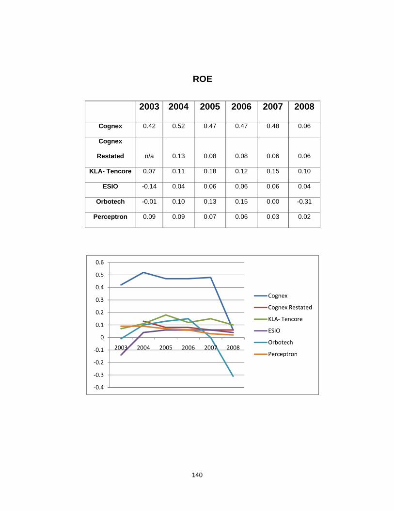
140
ROE
2003 2004 2005 2006 2007 2008
Cognex 0.42 0.52 0.47 0.47 0.48 0.06
Cognex
Restated n/a 0.13 0.08 0.08 0.06 0.06
KLA- Tencore 0.07 0.11 0.18 0.12 0.15 0.10
ESIO -0.14 0.04 0.06 0.06 0.06 0.04
Orbotech -0.01 0.10 0.13 0.15 0.00 -0.31
Perceptron 0.09 0.09 0.07 0.06 0.03 0.02
‐0.4
‐0.3
‐0.2
‐0.1
0
0.1
0.2
0.3
0.4
0.5
0.6
2003 2004 2005 2006 2007 2008
Cognex
Cognex Restated
KLA‐ Tencore
ESIO
Orbotech
Perceptron
141
Conclusion
When comparing Cognex’s profitability ratios to their competitors, it is clear where Cognex
stands. The firm is the leader of the industry when comparing operating profit margin, gross profit
margin and net profit margin. However, Cognex lags behind its competitors when it comes to the
operating expense ratio and asset turnover ratio. The firm’s asset turnover might be slightly below
average, but it has been consistent up until 2007. Cognex’s restated ROA ratio appears to be
inconsistent with the industry average, but they have obtained one of the largest returns on equity in
the industry.
Growth Rate Ratios
Growth rates are used to help firms evaluate the future growth potential of the business and
whether or not extra financing will be needed to maintain operations of the firm. These rates allow
managers to ensure the company is maintaining appropriate sales growth with the applied capital
structure. If income continues to grow quickly with no increase in debt, the debt to equity ratio may
decrease substantially, leading to a cheaper cost of financing. This may prompt managers to select
investment projects that may cause problems with the structure of capital within the firm and upset
normal business operations. The two growth rates used in analyzing equity of a firm include the
internal growth rate and the sustainable growth rate. Just as managers work to increase profits, they
must manage the internal operations carefully to prevent strategic error.
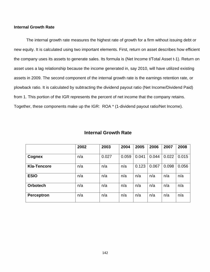
142
Internal Growth Rate
The internal growth rate measures the highest rate of growth for a firm without issuing debt or
new equity. It is calculated using two important elements. First, return on asset describes how efficient
the company uses its assets to generate sales. Its formula is (Net Income t/Total Asset t-1). Return on
asset uses a lag relationship because the income generated in, say 2010, will have utilized existing
assets in 2009. The second component of the internal growth rate is the earnings retention rate, or
plowback ratio. It is calculated by subtracting the dividend payout ratio (Net Income/Dividend Paid)
from 1. This portion of the IGR represents the percent of net income that the company retains.
Together, these components make up the IGR: ROA * (1-dividend payout ratio/Net Income).
Internal Growth Rate
2002 2003 2004 2005 2006 2007 2008
Cognex n/a 0.027 0.059 0.041 0.044 0.022 0.015
Kla-Tencore n/a n/a n/a 0.123 0.067 0.098 0.056
ESIO n/a n/a n/a n/a n/a n/a n/a
Orbotech n/a n/a n/a n/a n/a n/a n/a
Perceptron n/a n/a n/a n/a n/a n/a n/a
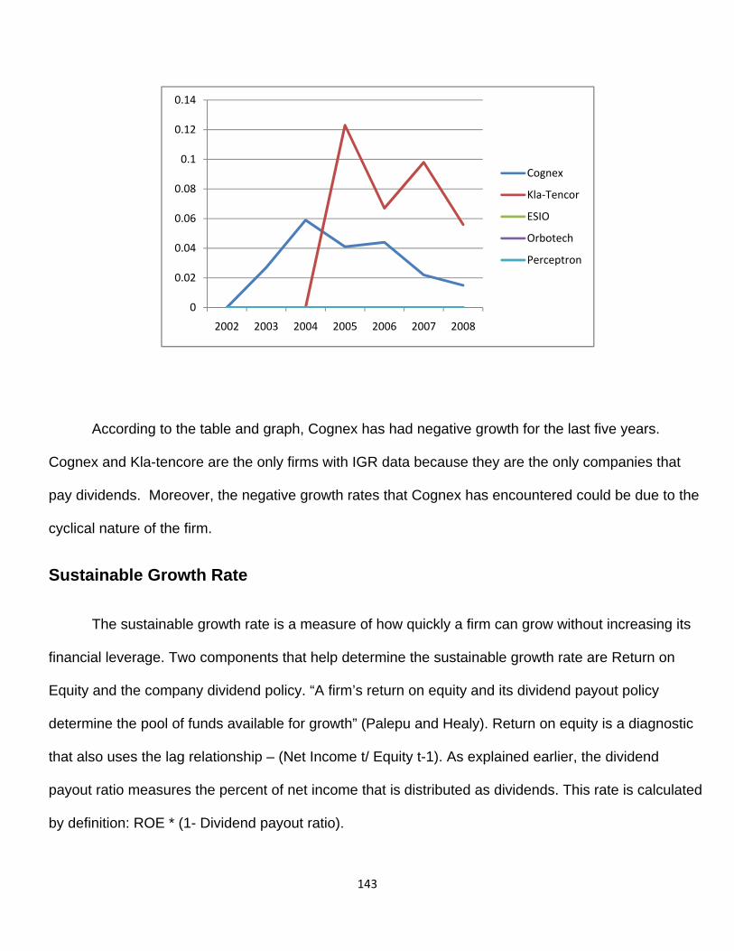
143
According to the table and graph, Cognex has had negative growth for the last five years.
Cognex and Kla-tencore are the only firms with IGR data because they are the only companies that
pay dividends. Moreover, the negative growth rates that Cognex has encountered could be due to the
cyclical nature of the firm.
Sustainable Growth Rate
The sustainable growth rate is a measure of how quickly a firm can grow without increasing its
financial leverage. Two components that help determine the sustainable growth rate are Return on
Equity and the company dividend policy. “A firm’s return on equity and its dividend payout policy
determine the pool of funds available for growth” (Palepu and Healy). Return on equity is a diagnostic
that also uses the lag relationship – (Net Income t/ Equity t-1). As explained earlier, the dividend
payout ratio measures the percent of net income that is distributed as dividends. This rate is calculated
by definition: ROE * (1- Dividend payout ratio).
0
0.02
0.04
0.06
0.08
0.1
0.12
0.14
2002 2003 2004 2005 2006 2007 2008
Cognex
Kla‐Tencor
ESIO
Orbotech
Perceptron
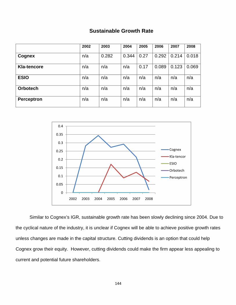
144
Sustainable Growth Rate
2002 2003 2004 2005 2006 2007 2008
Cognex n/a 0.282 0.344 0.27 0.292 0.214 0.018
Kla-tencore n/a n/a n/a 0.17 0.089 0.123 0.069
ESIO n/a n/a n/a n/a n/a n/a n/a
Orbotech n/a n/a n/a n/a n/a n/a n/a
Perceptron n/a n/a n/a n/a n/a n/a n/a
Similar to Cognex’s IGR, sustainable growth rate has been slowly declining since 2004. Due to
the cyclical nature of the industry, it is unclear if Cognex will be able to achieve positive growth rates
unless changes are made in the capital structure. Cutting dividends is an option that could help
Cognex grow their equity. However, cutting dividends could make the firm appear less appealing to
current and potential future shareholders.
0
0.05
0.1
0.15
0.2
0.25
0.3
0.35
0.4
2002 2003 2004 2005 2006 2007 2008
Cognex
Kla‐tencor
ESIO
Orbotech
Perceptron
145
Conclusion
Cognex must change their financial policies if they plan on staying competitive in this industry.
When the economy is booming, growth is easily obtainable. Since we are in a worldwide recession,
however, this cyclical industry will have a hard time growing their equity. Therefore, industry growth is
likely to be lower in years to come.
Capital Structure Analysis
Capital structure ratios are used to determine the leverage within a particular firm. These ratios
can also be used to explain the credit rating of a firm, as well as the firm’s ability to pay off its debts
and interest. The capital structure ratios allow analysts to understand how a firm finances its assets. A
firm’s assets can be financed either through debt which is by obtaining loans and bonds, or through
equity which is selling shares of the company’s stock. Firm’s that rely heavily on debt financing will
have lower credit ratings ultimately making it more difficult and expensive for them to borrow money.
Firm’s that rely more on equity financing are highly capable of paying off their liabilities and interest.
The three primary measures of capital structure are the debt to equity ratio, times interest earned, and
debt service margin.
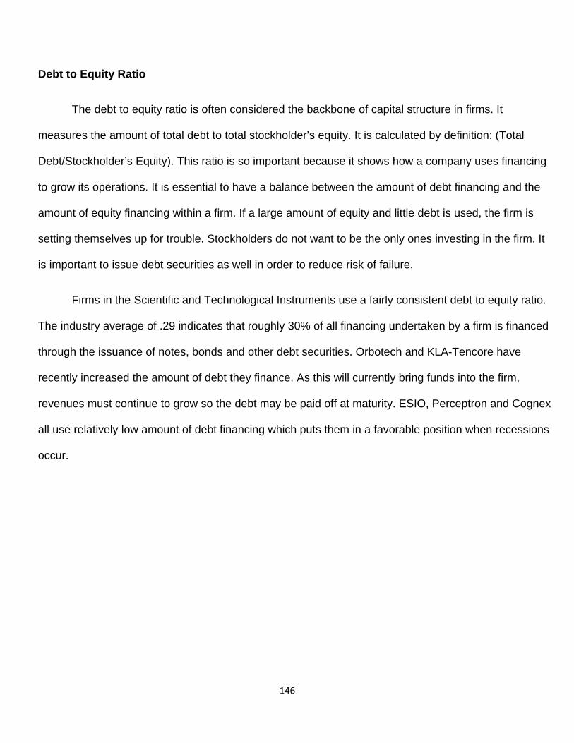
146
Debt to Equity Ratio
The debt to equity ratio is often considered the backbone of capital structure in firms. It
measures the amount of total debt to total stockholder’s equity. It is calculated by definition: (Total
Debt/Stockholder’s Equity). This ratio is so important because it shows how a company uses financing
to grow its operations. It is essential to have a balance between the amount of debt financing and the
amount of equity financing within a firm. If a large amount of equity and little debt is used, the firm is
setting themselves up for trouble. Stockholders do not want to be the only ones investing in the firm. It
is important to issue debt securities as well in order to reduce risk of failure.
Firms in the Scientific and Technological Instruments use a fairly consistent debt to equity ratio.
The industry average of .29 indicates that roughly 30% of all financing undertaken by a firm is financed
through the issuance of notes, bonds and other debt securities. Orbotech and KLA-Tencore have
recently increased the amount of debt they finance. As this will currently bring funds into the firm,
revenues must continue to grow so the debt may be paid off at maturity. ESIO, Perceptron and Cognex
all use relatively low amount of debt financing which puts them in a favorable position when recessions
occur.
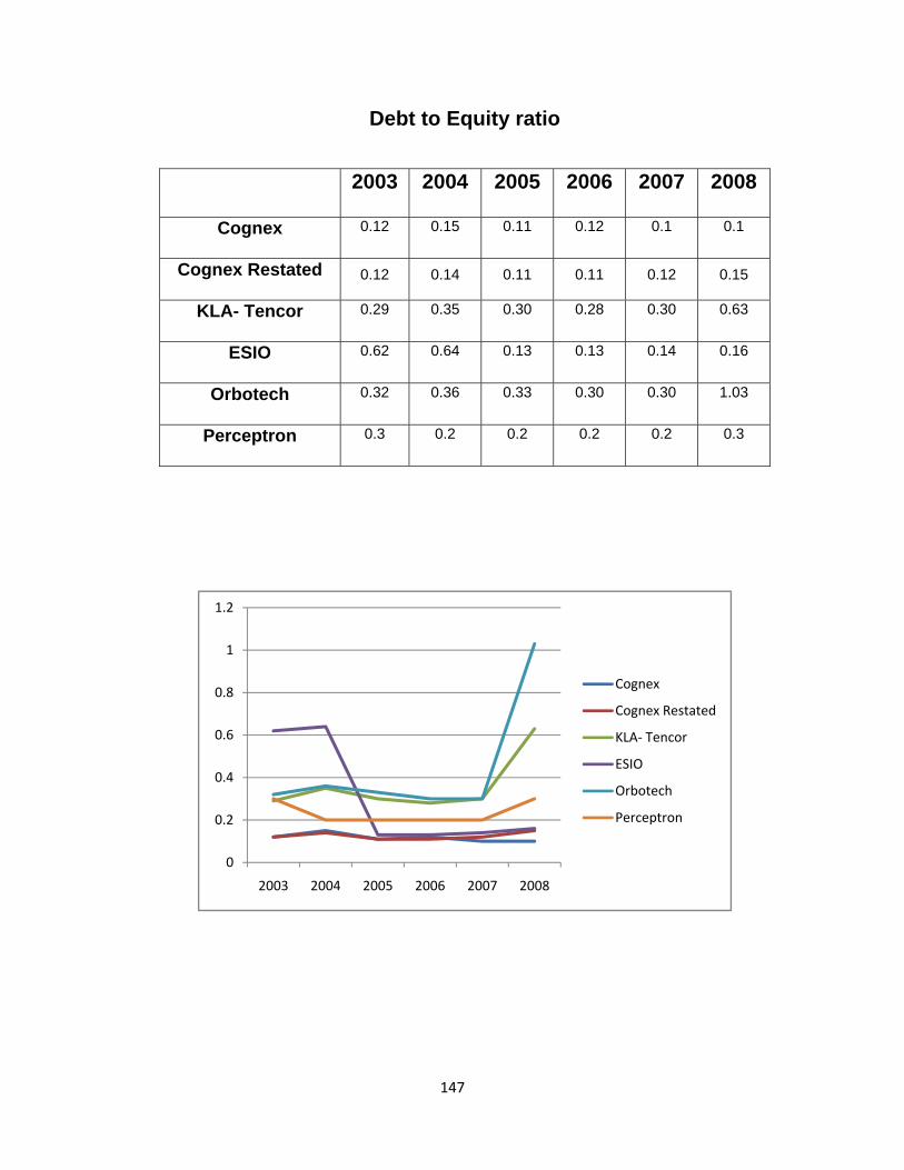
147
Debt to Equity ratio
2003 2004 2005 2006 2007 2008
Cognex 0.12 0.15 0.11 0.12 0.1 0.1
Cognex Restated 0.12 0.14 0.11 0.11 0.12 0.15
KLA- Tencor 0.29 0.35 0.30 0.28 0.30 0.63
ESIO 0.62 0.64 0.13 0.13 0.14 0.16
Orbotech 0.32 0.36 0.33 0.30 0.30 1.03
Perceptron 0.3 0.2 0.2 0.2 0.2 0.3
0
0.2
0.4
0.6
0.8
1
1.2
2003 2004 2005 2006 2007 2008
Cognex
Cognex Restated
KLA‐ Tencor
ESIO
Orbotech
Perceptron
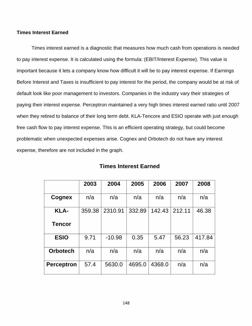
148
Times Interest Earned
Times interest earned is a diagnostic that measures how much cash from operations is needed
to pay interest expense. It is calculated using the formula: (EBIT/Interest Expense). This value is
important because it lets a company know how difficult it will be to pay interest expense. If Earnings
Before Interest and Taxes is insufficient to pay interest for the period, the company would be at risk of
default look like poor management to investors. Companies in the industry vary their strategies of
paying their interest expense. Perceptron maintained a very high times interest earned ratio until 2007
when they retired to balance of their long term debt. KLA-Tencore and ESIO operate with just enough
free cash flow to pay interest expense. This is an efficient operating strategy, but could become
problematic when unexpected expenses arise. Cognex and Orbotech do not have any interest
expense, therefore are not included in the graph.
Times Interest Earned
2003 2004 2005 2006 2007 2008
Cognex n/a n/a n/a n/a n/a n/a
KLA-
Tencor
359.38 2310.91 332.89 142.43 212.11 46.38
ESIO 9.71 -10.98 0.35 5.47 56.23 417.84
Orbotech n/a n/a n/a n/a n/a n/a
Perceptron 57.4 5630.0 4695.0 4368.0 n/a n/a
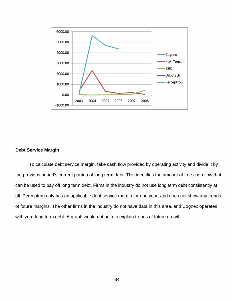
149
Debt Service Margin
To calculate debt service margin, take cash flow provided by operating activity and divide it by
the previous period’s current portion of long term debt. This identifies the amount of free cash flow that
can be used to pay off long term debt. Firms in the industry do not use long term debt consistently at
all. Perceptron only has an applicable debt service margin for one year, and does not show any trends
of future margins. The other firms in the industry do not have data in this area, and Cognex operates
with zero long term debt. A graph would not help to explain trends of future growth.
‐1000.00
0.00
1000.00
2000.00
3000.00
4000.00
5000.00
6000.00
2003 2004 2005 2006 2007 2008
Cognex
KLA‐ Tencor
ESIO
Orbotech
Perceptron
150
Z-Scores
Altman’s Z-score is used to compute bankruptcy score of a firm using five weighted variables
(Palepu & Healy). The Z-score is used as a credit score indicator used to compare the credit risk
among rival firms. A firm achieves a better credit rating the higher the Z-score. For example, a firm
with a Z-score above 3 will have a much lower interest rate than a firm with a 2. A firm with a Z-score
above 2.67 is considered good. Moreover, a firm with a Z-score between 1.81 and 2.67 is considered
to be uncertain. Finally, a firm with a score below 1.81 is predicted to go bankrupt. The following
formula below uses the five weighted variables to calculate the Altman’s Z-score.
1.2(Net Working Capital/Total Assets) +1.4(Retained Earnings/Total Assets) + 3.3(Earnings before Interest and Taxes/Total Assets) + 0.6(Market Value of Equity/Book Value of Liabilities) + 1.0(Sales/Total Assets) = Altman’s Z-Score
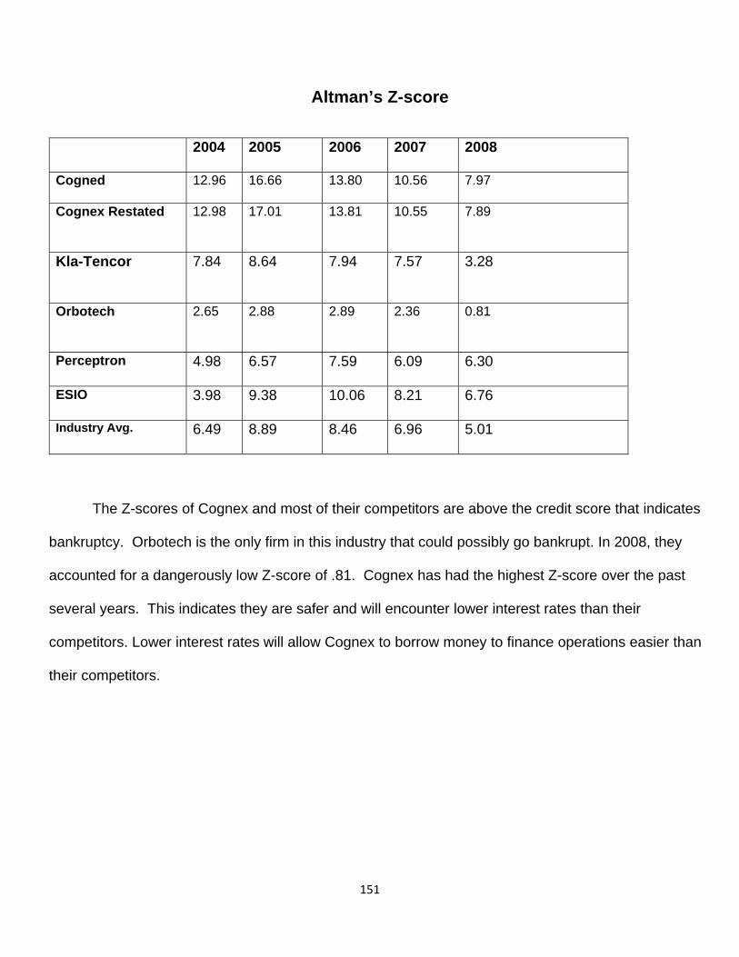
151
Altman’s Z-score
2004 2005 2006 2007 2008
Cogned 12.96 16.66 13.80 10.56 7.97
Cognex Restated 12.98
17.01
13.81
10.55
7.89
Kla-Tencor 7.84
8.64
7.94
7.57
3.28
Orbotech 2.65
2.88
2.89
2.36
0.81
Perceptron 4.98 6.57 7.59 6.09 6.30
ESIO 3.98 9.38 10.06 8.21 6.76
Industry Avg. 6.49 8.89 8.46 6.96 5.01
The Z-scores of Cognex and most of their competitors are above the credit score that indicates
bankruptcy. Orbotech is the only firm in this industry that could possibly go bankrupt. In 2008, they
accounted for a dangerously low Z-score of .81. Cognex has had the highest Z-score over the past
several years. This indicates they are safer and will encounter lower interest rates than their
competitors. Lower interest rates will allow Cognex to borrow money to finance operations easier than
their competitors.
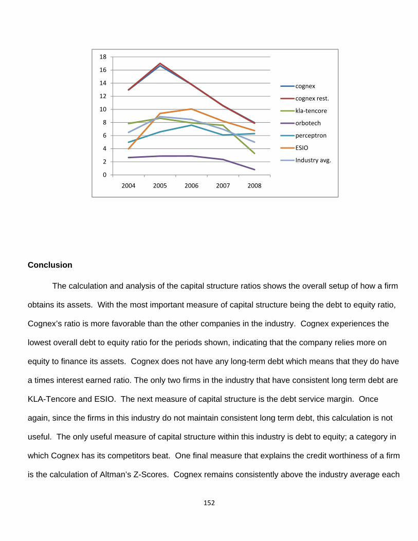
152
Conclusion
The calculation and analysis of the capital structure ratios shows the overall setup of how a firm
obtains its assets. With the most important measure of capital structure being the debt to equity ratio,
Cognex’s ratio is more favorable than the other companies in the industry. Cognex experiences the
lowest overall debt to equity ratio for the periods shown, indicating that the company relies more on
equity to finance its assets. Cognex does not have any long-term debt which means that they do have
a times interest earned ratio. The only two firms in the industry that have consistent long term debt are
KLA-Tencore and ESIO. The next measure of capital structure is the debt service margin. Once
again, since the firms in this industry do not maintain consistent long term debt, this calculation is not
useful. The only useful measure of capital structure within this industry is debt to equity; a category in
which Cognex has its competitors beat. One final measure that explains the credit worthiness of a firm
is the calculation of Altman’s Z-Scores. Cognex remains consistently above the industry average each
0
2
4
6
8
10
12
14
16
18
2004 2005 2006 2007 2008
cognex
cognex rest.
kla‐tencore
orbotech
perceptron
ESIO
Industry avg.
153
year in this calculation. This indicates this higher level of safety, making it easier for them to obtain
lower interest rates when borrowing. The company’s high Z-Score along with their industry leading
debt to equity ratios shows that Cognex is the safest and more trustworthy firm in the industry.
Financial Statement Forecasting
Forecasting is a method for the company to predict future profits, costs, expenses, and other
aspects of the business activities by reviewing and analyzing present and historical data. By reviewing
this information, analysts are able to make educated estimates of future trends and market estimates.
These estimates are prepared using the previously discovered ratios, growth rates, and averages
throughout the industry and past tendencies of the market with regard to the condition of the economy.
With the current recession affecting the market greatly, a company can research performance in past
recessions to estimate future financials.
Income Statement Forecasting:
In the process of financial statement forecasting, one must begin with the income statement.
This is the most important, due to the amount of referencing to sales. Additionally most of the
information calculated on the income statement greatly affects many elements of the balance sheet
and the statement of cash flows. Therefore forecasting the income statement accurately is imperative,
to have a successful and viable prospective analysis.
To begin forecasting the income statement analysts must first look at sales and find a current
growth rate. The current recession has affected the world economy and most industries and their
154
related markets. However this will not greatly affect this industry due to the amount of long term
contracts being upheld. Therefore the current recession should be taken into a mild consideration.
When forecasting sales, the recession of 2002 was discussed and implemented into our forecast as
well as information from 2000 to 2008. Upon examining past sales information we discovered a sales
pattern of growth for 4 to 5 years with a slight decline on average of 6 percent following the years of
growth. This can be explained by new technological innovations and advancements in the industry.
When Cognex sales did fall one of the competitors sales grew indicating a new innovation, and core
competency. This last occurred in the industry during the year of 2007 were sales declined by 6.13
percent. The constant trend of Cognex’s sales growth and the industry patterns induces the
assumption that Cognex’s sales will continue to grow at a rate of 6 percent till the year of 2012 where
sales will drop by 6 percent. We also concluded that following a drop in sales, sales grew at a more
rapid pace normally at a rate of 7.5 percent. This is most likely explained by the new technological
innovation in the company leading to an increase in long term contracts for the company. Following
sales will then level out to its average 6 percent and then fall again in the year 2018, followed by an
increase in 2019.
Secondly we forecasted our gross profit. In forecasting our gross profit we averaged the past 6
years of gross profit in relation to sales. In doing so we determined that gross profit was 71 percent of
sales. However as with the pattern in sales, when sales fell our gross profit fell also due to new
technological innovation in the industry. During the years of 2012 and 2017 a decline in sales took
place, implementing a gross profit reduction of 6 - 7 percent,. This allows analysts to make the
assumption that Cognex should not have any problems fulfilling any short term liabilities due to the
absence of liquidity.
Our next forecast was over the cost of goods sold. We found that gross profit gave us a more
155
accurate prediction of future growth on earnings as opposed to using cost of revenue trends.
Additionally the fact that our company mainly relies on a differentiated strategy, we concluded that our
costs were not of as of importance, in comparison to sales. Therefore we forecasted our sales and
gross profit first and then subtracted gross profit from sales to attain our cost of goods sold. As well as
with sales and gross profit, in the years of 2012 and 2017 the reduction of sales and gross profit led to
the reduction of cost of goods sold.
Following Gross Profit we forecasted research and development. We inferred that the amount
of money allocated to research and development would remain as a percentage of sales, due to the
fact that without any sales we would have no money to allocate to research and development.
However during the years that experienced a decrease in growth, we did not allocated less to research
and development, in order to create a new competitive advantage for the company. When examining
the previous years of allocation to research and development we discovered that on average 14
percent of current year sales we dedicated to research and development.
Selling, General and Administrative Expenses was next to forecast on the income statement.
We again found this as a percentage of sales. These throughout the previous years continued to grow
at a constant rate, even throughout the down years. There were no outliers and all very close to an
average of 40.2 percent of sales. This high percentage results because of the extensive labor and
servicing included in selling these products, and the large amounts of commission paid out to
employees.
In forecasting operating income as a percentage of sales yielded an average of 14% OI/sales.
We felt it best not to forecast this average but rather add in to our forecasted Gross Profit the cost of
revenue, research and development, selling general and administrative expenses to come up with a

156
reasonable estimate of OI. This allowed us to get the most accurate prediction of operating income,
because all of these must add up to give us total revenue. Simply finding the operating income by an
average percentage of sales would not allow an accurate operating income or loss.
The last line of the income statement to be forecasted is net income. Net income is computed
by taking operating income and adding or subtracting total other income/ expenses, next adding or
subtracting your foreign currency gain/ loss, and subtracting your income tax expense. However a
foreign currency gain or loss was unable to forecast due to the large uncontrollable fluctuations in the
market. Cognex’s total other income normally occurs during services and installation that is
accompanied by a product at the purchasers request. With the sale of more technologically advanced
products, more and more customers are going to desire a professional to install the product, leading to
an increase in this income. We forecasted out total other income by using a recent average of 23%.
The forecasted amount of other income represented a 23% of the portion of OI for any given year.
Additionally we were able to forecast income tax expense for the reason that the expense is a percent
of the earnings before interest and taxes at 24%. Therefore we were able to find net income by
subtracting income tax expense from earnings before interest and taxes.
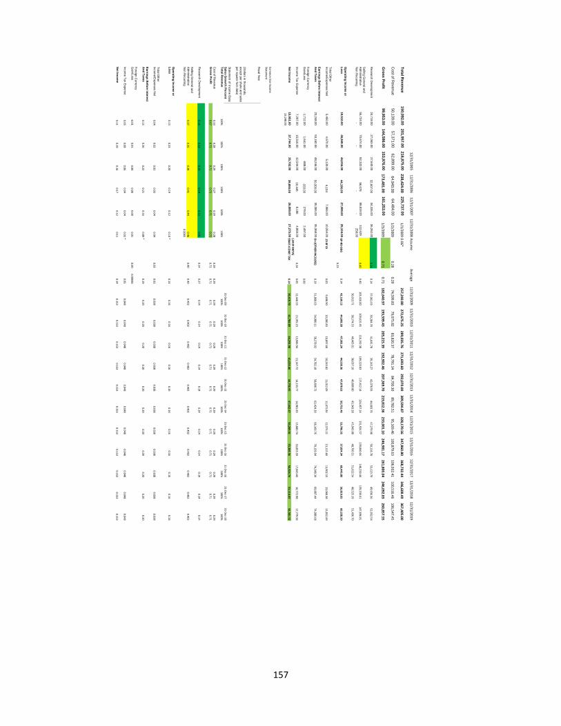
157
12/31/200512/31/2006
12/31/200712/31/2008
Assume
Average 12/31/2009
12/31/201012/31/2011
12/31/201212/31/2013
12/31/201412/31/2015
12/31/201612/31/2017
12/31/201812/31/2019
Total Revenue
150,092.00201,957.00
216,875.00238,424.00
225,737.001/1/2009
0.06*257,240.80
272,675.25289,035.76
271,693.60292,070.00
309,594.87328,170.56
347,860.80368,732.44
346,608.49367,405.00
Cost of R
evenue50,139.00
57,371.0062,899.00
64,943.0064,484.00
1/2/20090.28
0.2974,599.83
79,075.8283,820.37
78,791.1484,700.30
89,782.5195,169.46
100,879.63106,932.41
100,516.46106,547.45
Gross Profit
99,953.00144,586.00
153,976.00173,481.00
161,253.001/3/2009
0.710.71
182,640.97193,599.43
205,215.39192,902.46
207,369.70219,812.36
233,001.10246,981.17
261,800.04246,092.03
260,857.55
Research D
evelopment
24,719.0027,063.00
27,640.0032,607.00
34,335.0036,262.00
0.140.14
37,061.0339,284.70
41,641.7839,143.27
42,078.9344,603.76
47,279.9850,116.78
53,123.7949,936.36
52,932.54
Selling General and
Administrative
55,724.0070,674.00
82,332.0096,678
99,819.00112,629
0.400.40
103,410.80109,615.45
116,192.38109,220.83
117,412.14124,457.14
131,924.57139,840.04
148,230.44139,336.61
147,696.81N
on Recurring
- -
- -
258.0036,013.71
38,174.5340,465.01
38,037.1040,889.80
43,343.2845,943.88
48,700.5151,622.54
48,525.1951,436.70
Operating Incom
e or Loss
19,510.0046,849.00
44,004.0044,196.00
27,099.0025,104.00
GP‐RD
‐S&G
0.1442,169.13
44,699.2847,381.24
44,538.3647,878.63
50,751.4653,796.55
57,024.3460,445.80
56,819.0560,228.20
0.23
Total Other
Income/Expenses N
et5,450.00
4,670.005,130.00
6,104 7,986.00
10,264.00.23 0F O
I0.03
9,698.9010,280.83
10,897.6810,243.82
11,012.0911,672.84
12,373.2113,115.60
13,902.5313,068.38
13,852.49
Earnings Before Interest
And Taxes
23,248.0053,160.00
48,246.0050,300.00
35,085.0035,368.00
OI+(O
THER IN
C/LOSS)
0.1951,868.03
54,980.1158,278.92
54,782.1858,890.72
62,424.3066,169.76
70,139.9474,348.34
69,887.4474,080.68
Foreign Currency
Gain/Loss
-1,712.001,641.00
-888.00-333.00
279.002,497.00
0.00
Income Tax Expense
7,297.0015,516.00
12,544.0010,445
8,186 4,869.00
0.240.05
12,448.3313,195.23
13,986.9413,147.72
14,133.7714,981.83
15,880.7416,833.59
17,843.6016,772.98
17,779.36(.24 0F EBITA
)N
et Income
15,951.0037,744.00
35,702.0039,855.00
26,899.0027,275.00
EBIAT‐ICO
ME TA
X0.14
39,419.7041,784.89
44,291.9841,634.46
44,756.9547,442.47
50,289.0153,306.36
56,504.7453,114.45
56,301.3223,248.00
Common Size Incom
e Statem
ent
Fiscal Year
(Dollars in thousands,
except per share and sales per square foot data)
Statement of Incom
e Data:
Sales Grow
th Percent
31‐Dec‐09
31‐Dec‐10
31‐Dec‐11
31‐Dec‐12
31‐Dec‐13
31‐Dec‐14
31‐Dec‐15
31‐Dec‐16
31‐Dec‐16
31‐Dec‐17
31‐Dec‐18
Total Revenue
100%100%
100%100%
100%100%
100%100%
100%100%
100%100%
100%100%
100%100%
100%
Cost of R
evenue0.33
0.280.29
0.270.29
0.280.29
0.290.29
0.290.29
0.290.29
0.290.29
0.290.29
0.290.29
Gross Profit
0.670.72
0.710.73
0.710.72
0.710.71
0.710.71
0.710.71
0.710.71
0.710.71
0.710.71
0.71
Research D
evelopment
0.160.13
0.130.14
0.150.91
0.140.27
0.140.14
0.140.14
0.140.14
0.140.14
0.140.14
0.14
Selling General and
Administrative
0.370.35
0.380.41
0.440.46
0.400.40
0.4020.402
0.4020.402
0.4020.402
0.4020.402
0.4020.402
0.402N
on Recurring
0.0065
Operating Incom
e or Loss
0.130.23
0.200.19
0.120.10
*0.14
0.160.16
0.160.16
0.160.16
0.160.16
0.160.16
0.16
Total Other
Income/Expenses N
et0.04
0.020.02
0.030.04
0.040.03
0.030.038
0.0380.038
0.0380.038
0.0380.038
0.0380.038
0.0380.038
Earnings Before Interest
And Taxes
0.150.26
0.220.21
0.160.89
*0.19
0.200.20
0.200.20
0.200.20
0.200.20
0.200.20
0.20
Foreign Currency
Gain/Loss
‐0.010.01
0.000.00
0.000.01
0.000.00046
Income Tax Expense
0.050.08
0.060.04
0.040.02
*0.05
0.0480.048
0.0480.048
0.0480.048
0.0480.048
0.0480.048
0.048
Net Incom
e0.11
0.190.16
0.170.12
0.110.14
0.1530.153
0.1530.153
0.1530.153
0.1530.153
0.1530.153
0.153
158
Restated Income Statement Forecasting:
The main deviation between the original and restated income statement is the reduction in
goodwill and the increase in research and development by 20 percent. This expense on the restated
income statement reduced Cognexs operating profit and net income. Cognex’s net income overall fell
on average of 24 percent, and operating income fell from anywhere between 21 and 25 percent. Even
though goodwill and goodwill impairment cannot reasonably be predicted, based on these numbers
you can comprehend the significant difference the goodwill amortization expense will have on net
income, and emphasizes the importance of restating the financials.
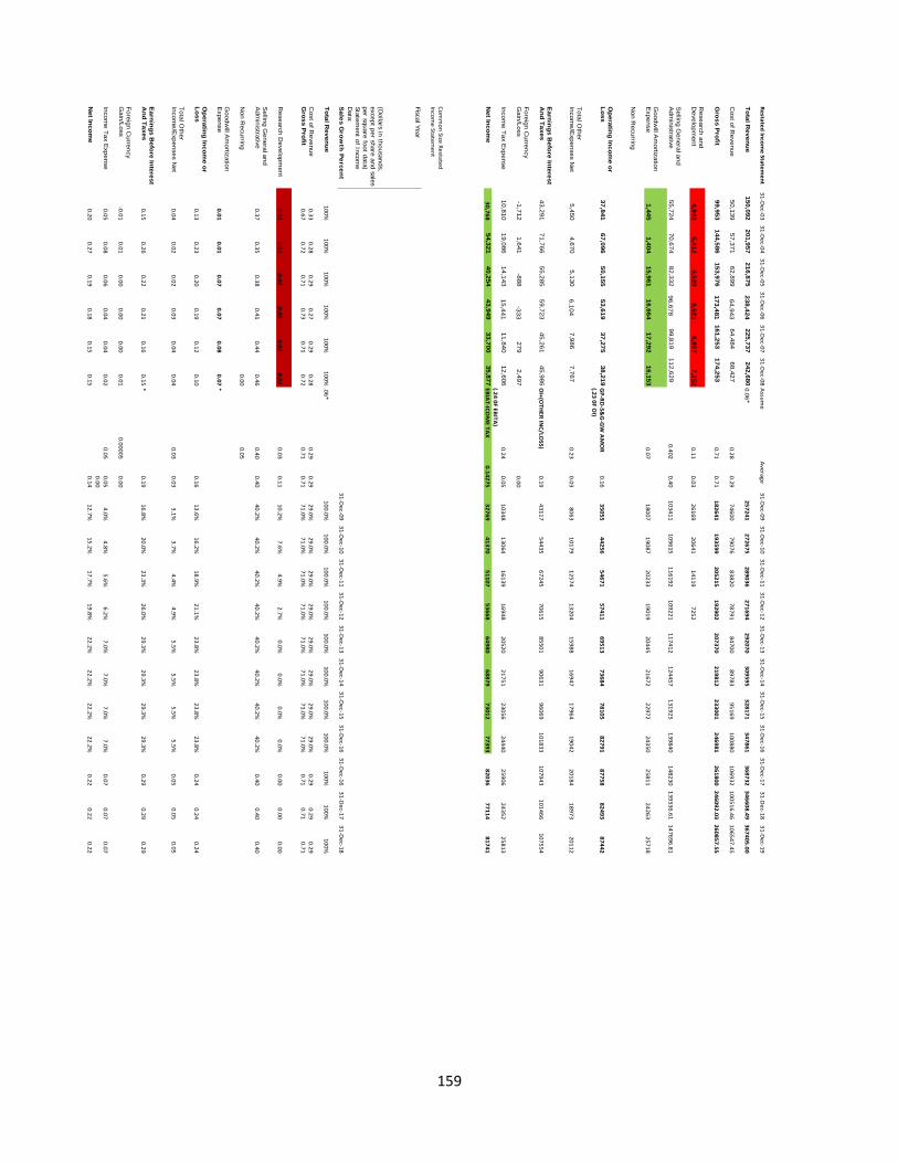
159
Restated Inco
me Statem
ent31‐D
ec‐0331‐D
ec‐0431‐D
ec‐0531‐D
ec‐0631‐D
ec‐0731‐D
ec‐08Assum
e Average
31‐Dec‐09
31‐Dec‐10
31‐Dec‐11
31‐Dec‐12
31‐Dec‐13
31‐Dec‐14
31‐Dec‐15
31‐Dec‐16
31‐Dec‐17
31‐Dec‐18
31‐Dec‐19
Total Revenue
150,092201,957
216,875238,424
225,737242,680
0.06*257241
272675289036
271694292070
309595328171
347861368732
346608.49367405.00
Cost of R
evenue50,139
57,37162,899
64,94364,484
68,427 0.28
0.2974600
7907683820
7879184700
8978395169
100880106932
100516.46106547.45
Gross P
rofit99,953
144,586153,976
173,481161,253
174,253 0.71
0.71182641
193599205215
192902207370
219812233001
246981261800
246092.03260857.55
Research and
Developm
ent4,943
5,4125,528
6,5216,867
7,2520.11
0.0326169
2064114119
7252
Selling G
eneral and A
dministrative
55,72470,674
82,33296,678
99,819 112,629
0.4020.40
103411109615
116192109221
117412124457
131925139840
148230139336.61
147696.81
Goodw
ill Am
ortization E
xpense1,445
1,40415,961
16,66417,292
16,1530.07
1800719087
2023319019
2044521672
2297224350
2581124263
25718
Non R
ecurring
Operating Incom
e or Loss
37,84167,096
50,15553,619
37,27538,219
GP‐R
D‐S&
G‐GW AMOR
0.1635055
4425654671
5741169513
7368478105
8279187758
8249387442
(.23 0F OI)
Total Other
Income/E
xpenses Net
5,4504,670
5,1306,104
7,986 7,767
0.230.03
806310179
1257413204
1598816947
1796419042
2018418973
20112
Earnings B
efore Interest A
nd Taxes43,291
71,76655,285
59,72345,261
45,986OI+(O
THER
INC/LO
SS)0.19
4311754435
6724570615
8550190631
96069101833
107943101466
107554
Foreign Currency
Gain/Loss
-1,7121,641
-888-333
2792,497
0.00
Income Tax E
xpense10,810
19,08614,143
15,44111,840
12,6060.24
0.0510348
1306416139
1694820520
2175123056
2444025906
2435225813
(.24 0F EBITA
)N
et Income
30,76854,321
40,25443,949
33,70035,877
EBIAT‐ICO
ME TA
X0.14275
3276941370
5110753668
6498068879
7301277393
8203677114
81741
Common Size R
estated Inco
me Statem
ent
Fiscal Year
(Dollars in thousands,
except per share and sales per square foot data)Statem
ent of Income
Data:
Sa
les G
row
th P
erce
nt
31‐Dec‐09
31‐Dec‐10
31‐Dec‐11
31‐Dec‐12
31‐Dec‐13
31‐Dec‐14
31‐Dec‐15
31 ‐Dec‐16
31‐Dec‐16
31‐Dec‐17
31‐Dec‐18
Total Revenue
100%100%
100%100%
100%100%
.06*100.0%
100.0%100.0%
100.0%100.0%
100.0%100.0%
100.0%100%
100%100%
Cost of R
evenue0.33
0.280.29
0.270.29
0.280.29
0.2929.0%
29.0%29.0%
29.0%29.0%
29.0%29.0%
29.0%0.29
0.290.29
Gross P
rofit0.67
0.720.71
0.730.71
0.720.71
0.7171.0%
71.0%71.0%
71.0%71.0%
71.0%71.0%
71.0%0.71
0.710.71
Research D
evelopment
0.030.03
0.030.03
0.030.03
0.030.11
10.2%7.6%
4.9%2.7%
0.0%0.0%
0.0%0.0%
0.000.00
0.00
Selling G
eneral and A
dministrative
0.370.35
0.380.41
0.440.46
0.400.40
40.2%40.2%
40.2%40.2%
40.2%40.2%
40.2%40.2%
0.400.40
0.40
Non R
ecurring0.00
0.05
Goodw
ill Am
ortization E
xpense0.01
0.010.07
0.070.08
0.07*
Operating Incom
e or Loss
0.130.23
0.200.19
0.120.10
0.1613.6%
16.2%18.9%
21.1%23.8%
23.8%23.8%
23.8%0.24
0.240.24
Total Other
Income/E
xpenses Net
0.040.02
0.020.03
0.040.04
0.030.03
3.1%3.7%
4.4%4.9%
5.5%5.5%
5.5%5.5%
0.050.05
0.05
Earnings B
efore Interest A
nd Taxes0.15
0.260.22
0.210.16
0.15*
0.1916.8%
20.0%23.3%
26.0%29.3%
29.3%29.3%
29.3%0.29
0.290.29
Foreign Currency
Gain/Loss
‐0.010.01
0.000.00
0.000.01
0.000050.00
Income Tax E
xpense0.05
0.080.06
0.040.04
0.020.05
0.054.0%
4.8%5.6%
6.2%7.0%
7.0%7.0%
7.0%0.07
0.070.07
0.00N
et Income
0.200.27
0.190.18
0.150.15
0.1412.7%
15.2%17.7%
19.8%22.2%
22.2%22.2%
22.2%0.22
0.220.22
160
Balance Sheet:
The balance sheet allows the company and investors a mental picture of the company’s current
financial position. Located on the balance sheet is information on a company’s assets, liabilities, and
owners equity. To keep the prospective analysis internally consistant it is necessary to keep time s on
the income statement consistent with those on the balance sheet. In forecasting out the balance sheet
it is important and useful to use internally consistent drivers form the income statement.
In order to forecast the balance sheet we forecasted Net Income. Then we would use our NI in
order to get your asset turnover. By doing so we were able to calculate an average Return on Assets
of .07, this allowed use to forecast Cognex’s total assets.
Next we were able to find current assets as a percentage of sales, at 56 percent. Net
receivables are found using the accounts receivables turnover of. Cognex’s turnover over the past 6
years averaged is 5.41; this number was consistent through most of the years. This allows Cognex to
conclude that it is collecting six times the amount of sales in cash in comparison to on account. Then
inventory was computed using the inventory turnover ratio. Here the cost of revenue is used divided
by inventory. Current inventory levels were consistent with sales and therefore an average inventory
turnover of 2.67 was concluded. A high inventory turnover can also imply that Cognex’s working cycle
is somewhat slow as we can see it takes Cognex 137 days to get rid of inventory.
After forecasting assets it is possible to forecast current liabilities. In order to forecast current
liabilities the current ratio was utilized. This led to an average of 5.36. By purchasing most current
assets and plants without debt financing, Cognex does not possess a lot of debt, and we can continue
to expect this kind of result in forecasting out their current liabilities.
Next is shareholders equity and first forecasted retained earnings, this was estimated by the
161
previous year’s retained earnings + current net income – current dividends. This formula allowed a
forecast of retained earnings. By acquiring attained earnings it is possible to find total shareholder
equity. This was cited by taking the previous year’s total shareholder equity and then adding it to
current retained earnings minus the previous year’s retained earnings. By obtaining total equity, total
equity was subtracted from total assets to give total liabilities.
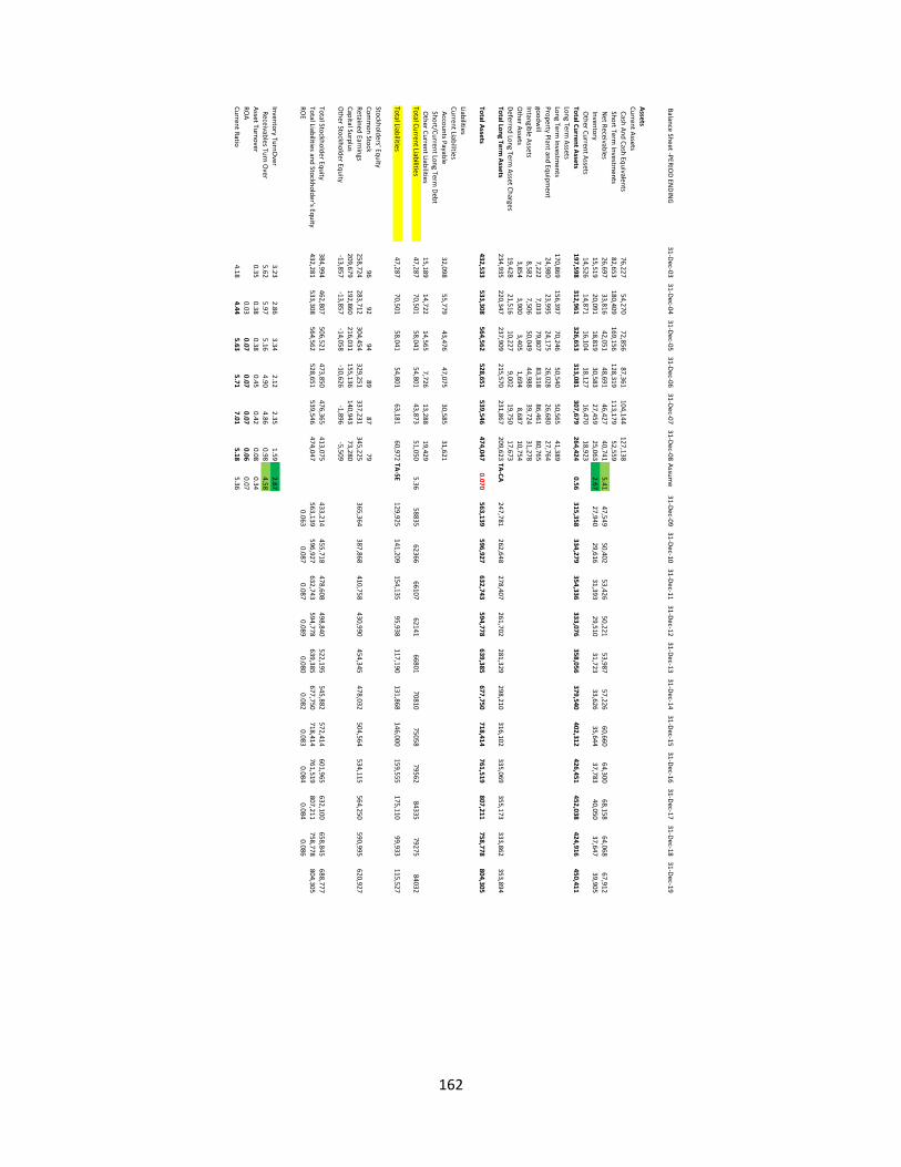
162
Balance Sheet ‐PERIOD EN
DING
31‐Dec‐03
31‐Dec‐04
31‐Dec‐05
31‐Dec‐06
31‐Dec‐07
31‐Dec‐08
Assum
e31‐D
ec‐0931‐D
ec‐1031‐D
ec‐1131‐D
ec‐1231‐D
ec‐1331‐D
ec‐1431‐D
ec‐1531‐D
ec‐1631‐D
ec‐1731‐D
ec‐1831‐D
ec‐19
Assets
Current AssetsCash And Cash Equivalents
76,22754,270
72,85687,361
104,144127,138
Short Term Investm
ents82,653
180,409169,156
128,319113,179
52,559Net Receivables
26,69733,816
42,05148,691
46,42740,741
5.4147,549
50,40253,426
50,22153,987
57,22660,660
64,30068,158
64,06867,912
Inventory15,519
20,09118,819
30,58327,459
25,0632.67
27,94029,616
31,39329,510
31,72333,626
35,64437,783
40,05037,647
39,905Other Current A
ssets14,526
14,87116,104
18,12716,470
18,923Total Current A
ssets197,598
312,961326,653
313,081307,679
264,4240.56
315,358334,279
354,336333,076
358,056379,540
402,312426,451
452,038424,916
450,411Long Term
AssetsLong Term
Investments
170,869156,397
70,24650,540
50,56541,389
Property Plant and Equipment
24,98023,995
24,17526,028
26,68027,764
goodwill
7,2227,033
79,80783,318
86,46180,765
Intangible Assets
8,5827,506
50,04944,988
39,72431,278
Other Assets
3,8543,900
3,4051,694
8,68710,754
Deferred Long Term
Asset Charges19,428
21,51610,227
9,00219,750
17,673Total Long Term
Assets
234,935220,347
237,909215,570
231,867209,623
TA‐CA
247,781262,648
278,407261,702
281,329298,210
316,102335,069
355,173333,862
353,894
Total Assets
432,533533,308
564,562528,651
539,546474,047
0.070563,139
596,927632,743
594,778639,385
677,750718,414
761,519807,211
758,778804,305
LiabilitiesCurrent LiabilitiesAccounts Payable
32,09855,779
43,47647,075
30,58531,621
Short/Current Long Term Debt
Other Current Liabilities
15,18914,722
14,5657,726
13,28819,429
Total Current Liabilities47,287
70,50158,041
54,80143,873
51,0505.36
5883562366
6610762141
6680170810
7505879562
8433579275
84032
Total Liabilities47,287
70,50158,041
54,80163,181
60,972TA
‐SE129,925
141,209154,135
95,938117,190
131,868146,000
159,555175,110
99,933115,527
Stockholders' Equity Com
mon Stock
9692
9489
8779
Retained Earnings258,724
283,712304,454
329,251337,231
345,225365,364
387,868410,758
430,990454,345
478,032504,564
534,115564,250
590,995620,927
Capital Surplus209,679
192,860216,031
155,136140,943
73,280Other Stockholder Equity
‐13,857‐13,857
‐14,058‐10,626
‐1,896‐5,509
Total Stockholder Equity384,994
462,807506,521
473,850476,365
413,075433,214
455,718478,608
498,840522,195
545,882572,414
601,965632,100
658,845688,777
Total Liabilities and Stockholder's Equity432,281
533,308564,562
528,651539,546
474,047563,139
596,927632,743
594,778639,385
677,750718,414
761,519807,211
758,778804,305
ROE
0.0630.087
0.0870.089
0.0800.082
0.0830.084
0.0840.086
Inventory TurnOver
3.232.86
3.342.12
2.351.59
2.67Receivables Turn O
ver5.62
5.975.16
4.904.86
0.984.58
Asset Turnover
0.350.38
0.380.45
0.420.08
0.34RO
A0.03
0.070.07
0.070.06
0.07Current Ratio
4.184.44
5.635.71
7.015.18
5.36
163
Restated Balance Sheet:
Upon restating our income statement, goodwill impairment was restated. In restating goodwill it
was imperative to reduce goodwill by 20 percent and therefore decreasing net income. However the
most affected area on the balance sheet was retained earnings, which upon re-forecasting was on
average 8% higher that the nominal retained earnings. The increase in retained earnings greatly
affected total owners equity as well, which on average was 7 % higher. The restatement of goodwill
will not affect the originally forecasted liabilities. The capitalization of 20 percent of research and
development, led to an increased in total assets from originally forecasted.
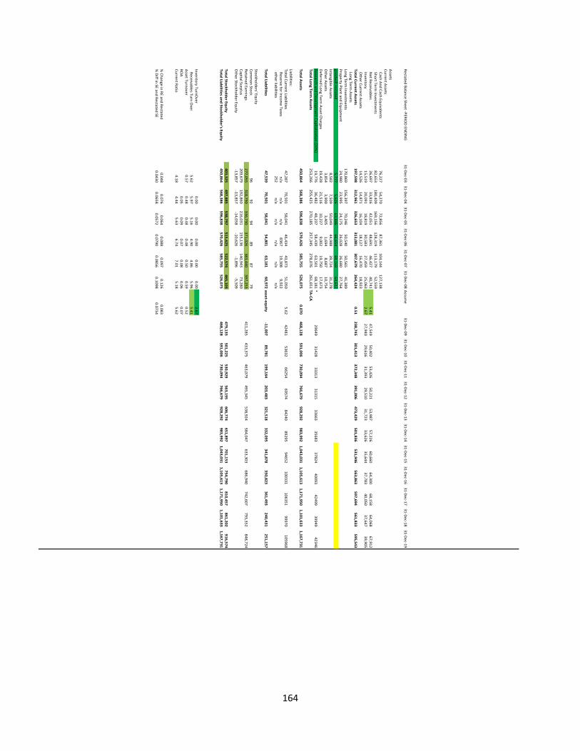
164
Restated
Balan
ce Sheet ‐PERIOD EN
DING
31‐Dec‐03
31‐Dec‐04
31‐Dec‐05
31‐Dec‐06
31‐Dec‐07
31‐Dec‐08
Assum
e31‐D
ec‐0931‐D
ec‐1031‐D
ec‐1131‐D
ec‐1231‐D
ec‐1331‐D
ec‐1431‐D
ec‐1531‐D
ec‐1631‐D
ec‐1731‐D
ec‐1831‐D
ec‐19
Assets
Curren
t Assets
Cash
And
Cash Equ
ivalents
76,22754,270
72,85687,361
104,144127,138
Short Term
Investm
ents
82,653180,409
169,156128,319
113,17952,559
Net R
eceivables
26,69733,816
42,05148,691
46,42740,741
5.4147,549
50,40253,426
50,22153,987
57,22660,660
64,30068,158
64,06867,912
Inven
tory
15,51920,091
18,81930,583
27,45925,063
2.6727,940
29,61631,393
29,51031,723
33,62635,644
37,78340,050
37,64739,905
Other C
urrent A
ssets14,526
14,87116,104
18,12716,470
18,923To
tal Curren
t Assets
197,598312,961
326,653313,081
307,679264,424
0.51238,745
301,413372,348
391,006473,429
501,836531,946
563,863597,694
561,833595,543
Long Term
Assets
Long Term
Investm
ents170,869
156,39770,246
50,54050,565
41,389Property Plant and
Equipm
ent24,980
23,99524,175
26,02826,680
27,764goodw
ill restated5,777
5,62663,846
66,65469,169
64,612Intan
gible A
ssets8,582
7,50950,049
44,98839,724
31,278Other A
ssets3,854
3,9003,405
1,6948,687
10,754Deferred
Long Term
Asset C
harges
19,42821,516
10,2279,002
19,75017,673
Research and
Develo
pmen
t Capitalizatio
n (20%
)19,776
36,48248,237
58,43963,501
68,181*
2964931428
3331331315
3366335683
3782440093
4249939949
42346To
tal Long Term
Assets
253,266255,425
270,185257,345
278,076261,651
TA‐CA
Total A
ssets450,864
568,386596,838
570,426585,755
526,0750.070
468,128591,006
730,094766,679
928,292983,992
1,043,0311,105,613
1,171,9501,101,633
1,167,731
Liabilities:To
tal Curren
t Liabilities
47,28770,501
58,04146,434
43,87351,050
5.6242481
5363266254
6957484240
8929594652
100331106351
99970105968
Reserve for Incom
e Taxesn/a
n/an/a
836719,308
9,922other liab
ilities252
n/an/a
n/an/a
n/a
Total Liab
ilities47,539
70,50158,041
54,80163,181
60,972asset‐eq
uity
‐11,00789,781
199,164203,483
321,518332,095
341,878350,823
361,493240,431
251,157
Stockho
lders' Equity
Common Sto
ck96
9294
8987
79Retained
Earnings277,055
318,790336,730
371,026383,440
397,253411,285
433,375463,079
495,345538,924
584,047633,303
686,940742,607
793,352848,724
Capital Surplus
209,679192,860
216,031155,136
140,94373,280
Other Sto
ckholder Equ
ity‐13,857
‐13,857‐14,058
‐10,626‐1,896
‐5,509
Total Sto
ckholder Eq
uity
403,325497,885
538,797515,625
522,574465,103
479,135501,225
530,929563,195
606,774651,897
701,153754,790
810,457861,202
916,574To
tal Liabilities an
d Sto
ckholder's Eq
uity
450,864568,386
596,838570,426
585,755526,075
468,128591,006
730,094766,679
928,292983,992
1,043,0311,105,613
1,171,9501,101,633
1,167,731
Inventory TurnO
ver0.00
0.000.00
0.000.00
2.67Receivab
les Turn Over
5.625.97
5.164.90
4.865.96
5.41Asset Tu
rnover
0.570.48
0.480.48
0.500.59
0.52ROA
0.050.09
0.070.08
0.060.07
Curren
t Ratio
4.184.44
5.636.74
7.015.18
5.62
% Chan
ge in RE and
Restated
0.0480.076
0.0640.088
0.0970.126
0.083% Diff in
SE and R
estated SE0.0430
0.06580.0572
0.07900.0856
0.10980.0734
165
Statement of Cash Flows:
The final forecast to complete is the statement of cash flows. This statement is most often the
most difficult and inaccurate of all the statements to forecast. By forecasting the statement of cash
flows investors can see the statement of cash flows which will offer insight on how proficient Cognex.
The statement of cash flows can be divided into three groups, first cash flow from operations, then net
cash flows from investing activities, and finally cash flows from financing activities.
In order to forecast our total cash flow from operating activities we found the ratios for: CFFO/
Net Sales, CFFO/ Operating Income, and CFFO/ Net Income. The following ratio that granted the
most accurate method of forecasting cash flow from operating activities was CFFO/ OI, and a ratio of
1.36. Net Income was able to be applied to the cash flow statement from the forecasted net income on
the income statement.
Next was the forecasting of the total cash flows from investing activities, in order to forecast this
unpredictable market the trend of CFFO from previous years was followed, however this was slightly
smaller due to the fact that we use more cash in operations as opposed to investing. Currently the
whole world is experiencing a recession and Cognex is not investing as much in long term
investments. In order to forecast for the recession a rate of -6.0 percent was chosen for recessionary
years, and a growth rate of 4.5 percent for a prospering year.
The concluding section of the statement of cash flows is the cash flow from financing activities.
Our dividend growth rate was calculated by averaging the last three year growth of dividends. When
examining the historical prices of our dividends, we concluded that every three years the price of the
dividend was increased. In order to forecast our dividend growth correctly we assumed a constant rate
for three years and then increased the dividend by 11 percent. We hesitated to increase the dividend

166
payment until 2011 to account for the current recession affecting payments. We concluded this was
adequate time for the market to re-establish itself.
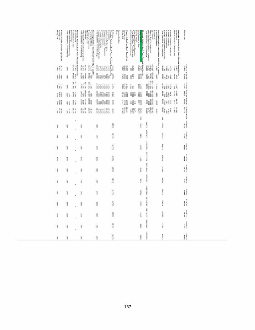
167
31‐Dec‐03
31‐Dec‐04
31‐Dec‐05
31‐Dec‐06
31‐Dec‐07
31‐Dec‐08
Assu
me
31‐Dec‐09
31‐Dec‐10
31‐Dec‐11
31‐Dec‐12
31‐Dec‐13
31‐Dec‐14
31‐Dec‐15
31‐Dec‐16
31‐Dec‐17
31‐Dec‐18
31‐Dec‐19
15,95137,744
35,70239,855
26,899 27,275
39,42041,785
44,29241,634
44,75747,442
50,28953,306
56,50553,114
56,301
5,4224,548
4,38711,667
11,358 12,695
9,64114,422
11,69012,166
4,850 15,385
-4,775-5,417
-5,7704,216
3,198 8,551
735-290
1,482-8,251
5,890 -1,929
5,833-3,642
1,048-10,178
124 -959
4575
364-996
-3,846-2,081
30,96463,176
42,76148,479
48,473 58,937
1.3657350.0
60791.064438.5
60572.265114.9
69022.073163.3
77553.182206.3
77273.981910.3
-2,462-3,120
-3,819-4,224
-4,635-6,012
Purchase of
investments
-165,534-805,621
-1,437,264-481,086
-277,876-120,622
149,429716,714
1,531,830541,023
292,213189,375
-11,787-123
-111,842-3,188
-1,0021,797
-30,354-92150
-2109552,525
8,700 64,538
*60665.72
63395.677459591.93676
62571.5335965074.39494
68002.7427163922.57815
66479.4812769471.05793
72944.6108375862.39526
-5,237-12,756
-14,960-15,058
-14,898-19,281
0.11‐19281
‐19281‐21402
‐21402‐21402
‐23756‐23756
‐23756‐26369
‐26369‐26369
20,65043,900
15525-75,937
-25,844-77,917
- -
- 1,413
241 1,671
15,41331,144
565-89,582
-40,501-95,527
-6602,120
-3,6453,083
111 -4,954
15,3634,290
18,58614,505
16,78322,994
Opening C
ash60,864
49,98054,270
72,85687,361
104,144Clo
sing C
ash76,227
54,27072,856
87,361104,144
127,138
Common Size C
ash
Flows
Net In
come
51.51%59.74%
83.49%82.21%
55.49%46.28%
68.74%68.74%
68.74%68.74%
68.74%68.74%
68.74%68.74%
68.74%68.74%
68.74%
17.51%7.20%
10.26%24.07%
23.43%21.54%
31.14%22.83%
27.34%25.10%
10.01%26.10%
‐15.42%‐8.57%
‐13.49%8.70%
6.60%14.51%
2.37%‐0.46%
3.47%‐17.02%
12.15%‐3.27%
18.84%‐5.76%
2.45%‐20.99%
0.26%‐1.63%
0.15%0.12%
0.85%‐2.05%
‐7.93%‐3.53%
100.00%100.00%
100.00%100.00%
100.00%100.00%
100%100%
100%100%
100%100%
100%100%
100%100%
100%
8.11%3.39%
18.10%‐8.04%
‐53.28%‐9.32%
545.34%874.25%
6813.29%‐915.92%
‐3193.98%‐186.90%
Maturity &
sale of investm
ents‐492.29%
‐777.77%‐7261.58%
1030.03%335.78%
293.43%38.83%
0.13%530.18%
‐6.07%‐11.52%
2.78%100.00%
100.00%100.00%
100.00%100.00%
100.00%100%
100%100%
100%100%
100%100%
100%100%
100%100%
‐33.98%‐40.96%
‐2647.79%16.81%
36.78%20.18%
**
**
**
**
**
*133.98%
140.96%2747.79%
84.77%63.81%
81.57%‐
‐‐
- -
- ‐1.58%
‐0.60%‐1.75%
100%100%
100%100%
100%100%
100%100%
100%100%
100%100%
100%100%
100%100%
100%
20.15%7.90%
25.51%16.60%
16.12%18.09%
Opening C
ash79.85%
92.10%74.49%
83.40%83.88%
81.91%Clo
sing C
ash100%
100%100%
100%100%
100%100%
100%100%
100%100%
100%100%
100%100%
100%100%
Changes In A
ccounts Receivables
Net Incom
e
Operating A
ctivities, Cash Flow
s Provided B
y or Used In
Depreciation
Other A
djustments To N
et Income
Changes In Liabilities
Changes In Inventories
Changes In O
ther Operating A
ctivitiesTotal C
ash Flow From
Operating
Investing Activities, C
ash Flows P
rovided By or U
sed InC
apital Expenditures
Maturity &
sale of investments
Other C
ashflows from
Investing Activities
Total Cash Flow
s From Investing
Total Cash Flow
s From Financing
Effect O
f Exchange R
ate Changes
Change In C
ash and Cash E
quivalents
Financing Activities, C
ash Flows P
rovided By or U
sed InD
ividends Paid
Sale P
urchase of Stock
Net B
orrowings
Other C
ash Flows from
Financing
Operating A
ctivities, Cash Flow
s Provided B
y or Used In:
Depreciation
Adjustm
ents To Net Incom
eC
hanges In Accounts R
eceivablesC
hanges In LiabilitiesC
hanges In InventoriesC
hanges In Other O
perating Activities
Total Cash Flow
From O
perating
Investing Activities, C
ash Flows P
rovided By or U
sed In:C
apital Expenditures
Purchase of investm
ents
Other C
ashflows from
Investing Activities
Total Cash Flow
s From Investing
Financing Activities, C
ash Flows P
rovided By or U
sed In:D
ividends Paid
Change In C
ash and Cash E
quivalents
Total Cash Flow
s From Financing
Sale P
urchase of Stock
Net B
orrowings
Other C
ash Flows from
Financing

168
Restated Statement of Cash Flows:
The only aspect of Cash Flows that is affected by the restatement is the total cash from
operating activities. Due to the fact that net income is affected by such a significant amount in the
previous two statements because of the goodwill impairment, when re-forecasting cash flow from
operating activities the amortization of goodwill is added in. By doing so it increases cash flow from
operating activities. By applying the amortization of goodwill cash flow from operating activities is able
to increase by 15.04 from the original forecast including recessionary years. The increase in this area
of the financial statement can greatly increase your net income, emphasizing the importance of
correctly forecasting the cash flow statement.
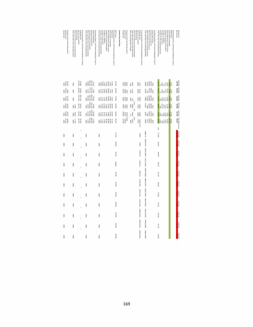
169
Restated C
F12/31/03
12/31/0412/31/05
12/31/0612/31/07
12/31/08Assu
me
12/31/0912/31/10
12/31/1112/31/12
12/31/1312/31/14
12/31/1512/31/16
12/31/1712/31/18
12/31/19Net Inco
me
30,76854,321
40,25443,949
33,70035,877
32,76941,370
51,10753,668
64,98068,879
73,01277,393
82,03677,114
81,741
Operatin
g Activities, Cash Flow
s Provided
By o
r Used In
:Depreciation
5,4224,548
4,38711,667
11,35812,695
Amortization
of Goodw
ill1,445
1,40415,961
16,66417,292
16,153Other A
djustmen
ts To Net Incom
e9,641
14,42211,690
12,1664,850
15,385Changes In
Accounts R
eceivables‐4,775
‐5,417‐5,770
4,2163,198
8,551Changes In
Liabilities735
‐2901,482
‐8,2515,890
‐1,929Changes In
Inventories5,833
‐3,6421,048
‐10,178124
‐959Changes In
Other O
perating A
ctivities45
75364
‐996‐3,846
‐2,081Total C
ash Flow From
Operatin
g Activities
49,11465,421
69,41669,237
72,56683,692
1.3657,350
60,79164,438
60,57265,115
69,02273,163
77,55382,206
77,27481,910
Investing Activities, C
ash Flows Provided B
y or Used In:
Capital Expen
ditures‐2462
‐3120‐3819
‐4224‐4635
‐6012Purch
ase of investments
‐165534‐805621
‐1437264‐481086
‐277876‐120622
Maturity &
sale of investm
ents
149429716714
1531830541023
292213189375
Other C
ashflows from
Investing Activities
‐11787‐123
‐111842‐3188
‐10021,797
Total Cash Flow
s From Investing A
ctivities‐30354
‐92150‐21095
52,525 8,700
64538
60665.7263395.6774
59591.9367662571.53359
65074.3949468002.74271
63922.5781566479.48127
69471.0579372944.61083
75862.39526
Financing Activities, Cash Flow
s Provided
By o
r Used In
:Dividends Paid
‐5237‐12756
‐14960‐15058
‐14898‐19281
0.11*‐19281
‐19281‐21401.91
‐21401.91‐21401.91
‐23756.1201‐23756.1201
‐23756.1201‐26369.29331
‐26369.29331‐26369.29331
Sale Purchase of Stock
2065043900
15525‐75937
‐25844‐77917
Net B
orrowings
‐ ‐
‐ Other C
ash Flows from
Financing A
ctivities1,413
241 1,671
Total Cash Flow
s From Finan
cing Activities
1541331144
565‐89582
‐40501‐95527
Effect Of Exchange R
ate Chan
ges‐660
2120‐3645
3,083 111
‐4954
Change In C
ash and Cash Eq
uivalents 15363
429018586
1450516783
22,994 Opening C
ash60864
4998054270
7285687361
104144Closin
g Cash
7622754270
7285687361
104144127138
Common Size C
ash Flo
ws
Net Inco
me
62.65%83.03%
57.99%63.48%
46.44%42.87%
57.14%68.05%
79.31%88.60%
99.79%99.79%
99.79%99.79%
99.79%99.79%
99.79%Operatin
g Activities, Cash Flow
s Provided
By o
r Used In
:Depreciation
11.04%6.95%
6.32%16.85%
15.65%15.17%
Amortization
of Good W
ill2.94%
2.15%22.99%
24.07%23.83%
19.30%Other A
djustmen
ts To Net Incom
e19.63%
22.04%16.84%
17.57%6.68%
18.38%Changes In
Accounts R
eceivables‐9.72%
‐8.28%‐8.31%
6.09%4.41%
10.22%Changes In
Liabilities1.50%
‐0.44%2.13%
‐11.92%8.12%
‐2.30%Changes In
Inventories11.88%
‐5.57%1.51%
‐14.70%0.17%
‐1.15%Changes In
Other O
perating A
ctivities0.09%
0.11%0.52%
‐1.44%‐5.30%
‐2.49%Total C
ash Flow From
Operatin
g Activities
100%100%
100%100%
100%100%
100%100%
100%100%
100%100%
100%100%
100%100%
100%
Investing Activities, C
ash Flows Provided B
y or Used In:
Capital Expen
ditures8.11%
3.39%18.10%
‐8.04%‐53.28%
‐9.32%Purch
ase of investments
545.34%874.25%
6813.29%‐915.92%
‐3193.98%‐186.90%
Maturity &
sale of investm
ents
‐492.29%‐777.77%
‐7261.58%1030.03%
335.78%293.43%
Other C
ashflows from
Investing Activities
38.83%0.13%
530.18%‐6.07%
‐11.52%2.78%
Total Cash Flow
s From Investing A
ctivities100%
100%100%
100%100%
100%100%
100%100%
100%100%
100%100%
100%100%
100%100%
Financing Activities, Cash Flow
s Provided
By o
r Used In
:Dividends Paid
‐33.98%‐40.96%
‐2647.79%16.81%
36.78%20.18%
**
**
**
**
**
*Sale Purch
ase of Stock133.98%
140.96%2747.79%
84.77%63.81%
81.57%Net B
orrowings
‐‐
‐‐
‐ ‐
Other C
ash Flows from
Financing A
ctivities‐1.58%
‐0.60%‐1.75%
Total Cash Flow
s From Finan
cing Activities
100%100%
100%100%
100%100%
100%100%
100%100%
100%100%
100%100%
100%100%
100%
Change In C
ash and Cash Eq
uivalents 20.15%
7.90%25.51%
16.60%16.12%
18.09%Opening C
ash79.85%
92.10%74.49%
83.40%83.88%
81.91%Closin
g Cash
100%100%
100%100%
100%100%
100%100%
100%100%
100%100%
100%100%
100%100%
100%

170
Cost of Debt
The cost of debt helps determine how risky a firm is compared to its competitors. It tends to be
a lower percentage compared to the cost of equity because equity holders have a higher risk of default
due to uncertain returns. In order to find the cost of debt, you must first find the weighted average cost
of debt for each liability. The weighted average cost of debt is calculated by multiplying the assigned
interest rate of each individual liability by the weight of the liability. The weight is found by taking the
amount of debt for each liability and dividing it by total liabilities. Once the weighted average cost of
debt is found for each liability, add the WACD for each liability together to find the cost of debt. The
table below describes this relationship.
Cost of Debt
Liabilities Debt Interest Rate Weight WACD
Accounts payable 6,780 0.48% 0.11 0.05%
Accrued Expenses 21,855 0.48% 0.36 0.17%
Accrued Income taxes 2,986 2.87% 0.05 0.14%
Deferred Revenue and
customer deposits 19,429 0.48% 0.32 0.15%
Reserve for Income taxes 9,922 2.87% 0.16 0.46%
Total Liabilities 60,972 0.97%
As the table above displays, Cognex has a limited amount of debt recorded on their balance
171
sheet. For accounts payable, accrued expenses, deferred revenue and customer deposits we used
the three month nonfinancial AA commercial paper rate found from the St. Louis Federal Reserve
(.48%). For Accrued Income taxes and reserve for income taxes we applied the 10 year yield for risk
free rates (2.87%). After adding the WACD for each liability together we found our cost of debt to be
.97%. The cost of debt for Cognex is lower than the risk free rate which seems unreasonable.
However, since Cognex does not finance their firm with large amounts of liabilities, there is little risk
present.
Cost of Equity:
To find a reasonable cost of Capital for a firm we must find a Cost of equity associated with that
firm. To estimate the Cost of equity we used a regression method using Capital Asset Pricing Model.
The model is a linear regression composed of a “required return on riskless assets plus a premium for
beta or systematic risk”(Palepu & Healy). To find a long run estimate of Cost of equity the return on a
10 year treasury bond can be used as a riskless return on assets. The systematic risk of beta
measures how well correlated a firm’s equity price moves with total market risk premium such as the
S&P 500. Firms which show a beta closer to 1 will show market values of equity that mimic economic
fluctuations, while firms with a low estimate of beta will be less sensitive to systematic market risk.
To estimate the firm’s systematic risk of beta we ran a linear regression composed
of the firm’s monthly market returns and a market return less monthly 3 month 1,2,5, and 10 year
Treasury Constant Maturity Rates. The MRP values of the monthly S&P market return less Treasury
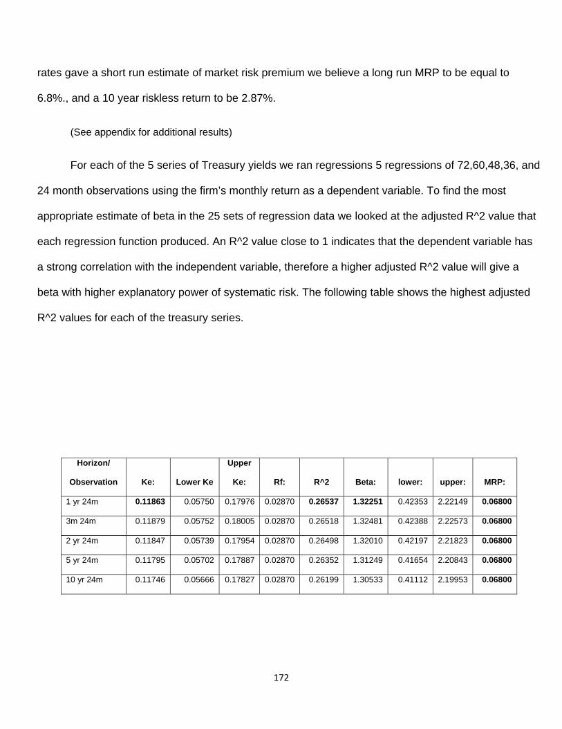
172
rates gave a short run estimate of market risk premium we believe a long run MRP to be equal to
6.8%., and a 10 year riskless return to be 2.87%.
(See appendix for additional results)
For each of the 5 series of Treasury yields we ran regressions 5 regressions of 72,60,48,36, and
24 month observations using the firm’s monthly return as a dependent variable. To find the most
appropriate estimate of beta in the 25 sets of regression data we looked at the adjusted R^2 value that
each regression function produced. An R^2 value close to 1 indicates that the dependent variable has
a strong correlation with the independent variable, therefore a higher adjusted R^2 value will give a
beta with higher explanatory power of systematic risk. The following table shows the highest adjusted
R^2 values for each of the treasury series.
Horizon/
Observation Ke: Lower Ke
Upper
Ke: Rf: R^2 Beta: lower: upper: MRP:
1 yr 24m 0.11863 0.05750 0.17976 0.02870 0.26537 1.32251 0.42353 2.22149 0.06800
3m 24m 0.11879 0.05752 0.18005 0.02870 0.26518 1.32481 0.42388 2.22573 0.06800
2 yr 24m 0.11847 0.05739 0.17954 0.02870 0.26498 1.32010 0.42197 2.21823 0.06800
5 yr 24m 0.11795 0.05702 0.17887 0.02870 0.26352 1.31249 0.41654 2.20843 0.06800
10 yr 24m 0.11746 0.05666 0.17827 0.02870 0.26199 1.30533 0.41112 2.19953 0.06800
173
The regressions of 24 month holdings produced the greatest R^2 for each holding period
showing that more recent observations have a higher explanatory power of market and treasury
returns. 1 year 24month series had the highest adjusted R^2 value with a beta of 1.32. 26.53% was the
highest explanatory power we obtained from all of the regressions, with this can estimate a Beta of
1.32. Our Estimate of Beta is higher than the published beta of 1.24. By looking at our R^ 2 values we
can see that shorter 1 year treasury yields had the highest explanatory power of Cognex’s returns,
although beta for the one 1 results remains reasonably stable around 1.3. Using our estimated
measure of systematic risk and all other variables, we estimated the cost of equity to be 11.86% using
CAPM. This estimate we believe is reasonable because of the relatively high explanatory power of
R^2, and it is within the 95% confidence interval of upper and lower bounds of the Beta intervals. We
believe this estimate of beta to be relevant because of the nature of Cognex’s production of goods
relative to market overall performance. A high measure of Beta risk illustrates that Cognex is settable
to overall market changes. Using CAPM we can show the calculations of cost of equity.
COE= Riskless rate of return + Beta risk *(Market Risk Premium) + Size Premium
11.86%= .0287+ ( 1.32 * .068)
Lower: 5.75%= .0287 + (.423 * .068)
Upper: 17.98%= .0287 + (2.22 * .068)
174
Size Adjusted:
The “Size Effect”, according to Palepu & Healy attempts to explain factors beyond just
systematic risk. The effect is defined as “smaller firms tend to generate higher returns in subsequent
periods”(Palepu & Healy). Data shows that relatively smaller firms have realized higher returns than
firms with significantly larger Market Cap, and this holds true if we assume that larger firms carry less
risk. The “Size effect” on cost of equity can be enacted by adding in a size premium to the CAPM
equation. Using Cognex’s Market Cap of 586.9 million we can find their size premium to be 2.7%.
Adding this premium into CAPM produces a cost of equity of 14.56%, however we believe the CAPM
method without the use of a size premium is a better estimate of cost of equity because Cognex’s
reasonable exposure to exposure to systematic risk.
COE= Riskless rate of return + Beta risk *(Market Risk Premium) + Size Premium
14.56%= .0287+ ( 1.32 * .068) + .027
Alternative Method:
The Alternative Cost of Equity method is one that will support a currently observed stock price
by equating the cost of equity to a price to book ratio. Although The “back door” method produced cost
of equity estimates that were within the upper and lower bounds of the CAPM regression, the costs
were relatively low compared to the regression estimations. Because of these low estimates we believe
the latter to be the best estimate of risk of Cognex. We calculated an average forecasted ROE of .091
and a average growth in book value of equity to be .0475. According to yahoo finance the current
175
Market to book ratio is 1.31.The value of Ke to equate the market to book ratio is shown below.
(M/B)-1= ROE-Ke/Ke-g
.31=.091-(.0807)/(.0807)-.0475
Ke= .0807
Weighted Average Cost of Capital
The WACC is an estimate of a firm’s assets biased on a combined measure of debt and equity.
By adding the weighted cost of equity and the cost of debt together we should be able to estimate a
firms cost of capital on both a before tax and after tax basis. The use of weight on the cost of debt and
equity let us take into account how much capital is financed either through debt or equity financing. The
denominator of our weight or MVA we defined as the sum of Cognex’s current market CAP of out
equity and the currently observed value of total liabilities. By multiplying our cost of dept by 1 less our
tax rate of 35% we found our WACC to be 10.81%, and our before tax WACC to be 10.81%. We can
support this observed estimate of WACC because we believe that our cost of capital will follow our cost
of equity rather than our cost of debt because our cost of equity is much more heavily weighted than
out cost of debt.
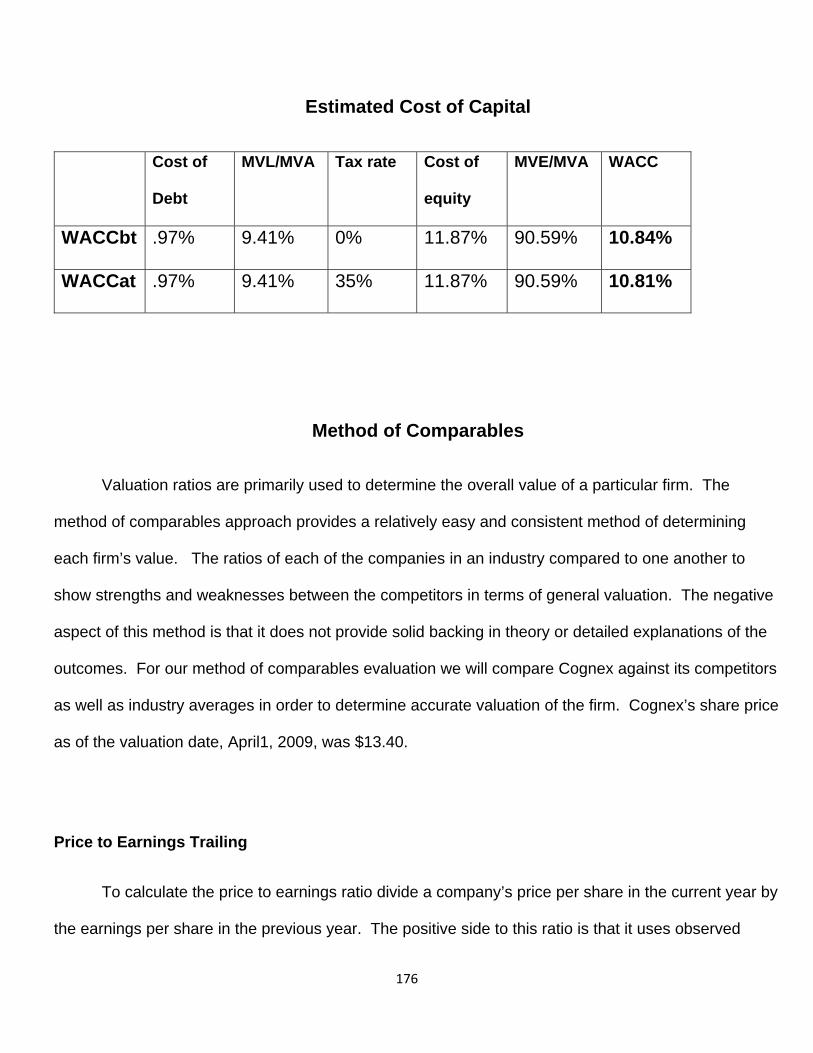
176
Estimated Cost of Capital
Cost of
Debt
MVL/MVA Tax rate Cost of
equity
MVE/MVA WACC
WACCbt .97% 9.41% 0% 11.87% 90.59% 10.84%
WACCat .97% 9.41% 35% 11.87% 90.59% 10.81%
Method of Comparables
Valuation ratios are primarily used to determine the overall value of a particular firm. The
method of comparables approach provides a relatively easy and consistent method of determining
each firm’s value. The ratios of each of the companies in an industry compared to one another to
show strengths and weaknesses between the competitors in terms of general valuation. The negative
aspect of this method is that it does not provide solid backing in theory or detailed explanations of the
outcomes. For our method of comparables evaluation we will compare Cognex against its competitors
as well as industry averages in order to determine accurate valuation of the firm. Cognex’s share price
as of the valuation date, April1, 2009, was $13.40.
Price to Earnings Trailing
To calculate the price to earnings ratio divide a company’s price per share in the current year by
the earnings per share in the previous year. The positive side to this ratio is that it uses observed
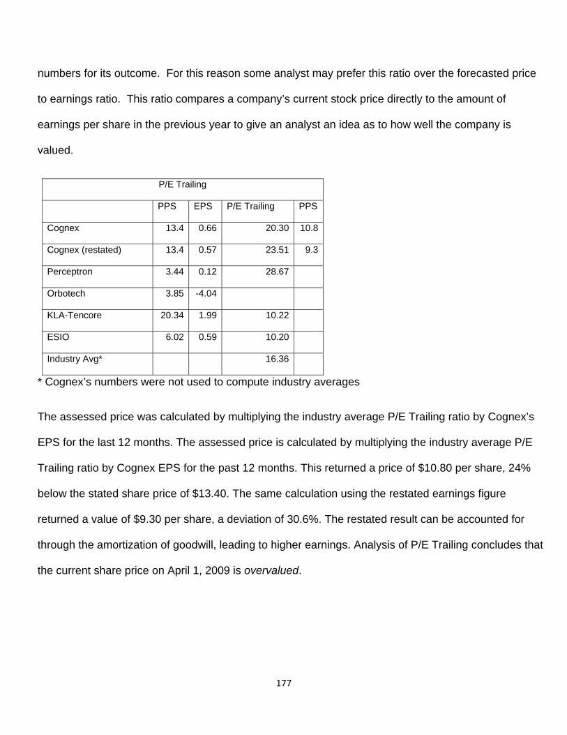
177
numbers for its outcome. For this reason some analyst may prefer this ratio over the forecasted price
to earnings ratio. This ratio compares a company’s current stock price directly to the amount of
earnings per share in the previous year to give an analyst an idea as to how well the company is
valued.
P/E Trailing
PPS EPS P/E Trailing PPS
Cognex 13.4 0.66 20.30 10.8
Cognex (restated) 13.4 0.57 23.51 9.3
Perceptron 3.44 0.12 28.67
Orbotech 3.85 -4.04
KLA-Tencore 20.34 1.99 10.22
ESIO 6.02 0.59 10.20
Industry Avg* 16.36
* Cognex’s numbers were not used to compute industry averages
The assessed price was calculated by multiplying the industry average P/E Trailing ratio by Cognex’s
EPS for the last 12 months. The assessed price is calculated by multiplying the industry average P/E
Trailing ratio by Cognex EPS for the past 12 months. This returned a price of $10.80 per share, 24%
below the stated share price of $13.40. The same calculation using the restated earnings figure
returned a value of $9.30 per share, a deviation of 30.6%. The restated result can be accounted for
through the amortization of goodwill, leading to higher earnings. Analysis of P/E Trailing concludes that
the current share price on April 1, 2009 is overvalued.

178
Price to Earnings Forecast
The price to earnings forecast ratio is closely related to the price to earnings trailing ratio in
terms of the calculation setup. This ratio is calculated by dividing the price per share in the current
year by the earnings per share in the future period. This calculation attempts to predict the price to
earnings ratio in the future period using forecast data. Since the earnings have been forecast for this
equation the level of potential error is considerably elevated.
P/E Forecast
PPS EPS(t+1) P/E forecast PPS
Cognex 13.4 0.99 13.54 10.35
Cognex (restated) 13.4 0.86 15.58 8.99
Perceptron 3.44 10.45
Orbotech 3.85
KLA-Tencore 20.34
ESIO 6.02
Industry Avg* 10.45
This calculation is similar to the P/E trailing, except forecasted net income from 2009 is used to
determine EPS. Since information on Orbotech, KLA-Tencore and ESIO were not available they were
not included in the analysis of this diagnostic. The industry average P/E forecast was multiplied by
forecasted Cognex ESP. The forward P/E ratio is clearly lower than the P/E trailing, which indicates
growth in the industry. The price per share is calculated similarly; multiply the industry average P/E
forecast by Cognex original and restated ESP. The original calculation results in a PPS of $10.35 while
the restated numbers indicate value at $8.99 per share. According to the model, the stated share price
is again overvalued.
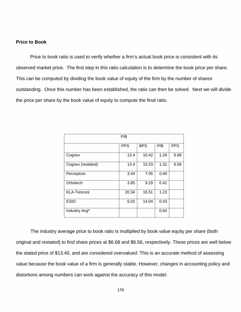
179
Price to Book
Price to book ratio is used to verify whether a firm’s actual book price is consistent with its
observed market price. The first step in this ratio calculation is to determine the book price per share.
This can be computed by dividing the book value of equity of the firm by the number of shares
outstanding. Once this number has been established, the ratio can then be solved. Next we will divide
the price per share by the book value of equity to compute the final ratio.
P/B
PPS BPS P/B PPS
Cognex 13.4 10.42 1.29 6.68
Cognex (restated) 13.4 10.23 1.31 6.56
Perceptron 3.44 7.05 0.49
Orbotech 3.85 9.29 0.41
KLA-Tencore 20.34 16.51 1.23
ESIO 6.02 14.04 0.43
Industry Avg* 0.64
The industry average price to book ratio is multiplied by book value equity per share (both
original and restated) to find share prices at $6.68 and $6.56, respectively. These prices are well below
the stated price of $13.40, and are considered overvalued. This is an accurate method of assessing
value because the book value of a firm is generally stable. However, changes in accounting policy and
distortions among numbers can work against the accuracy of this model.
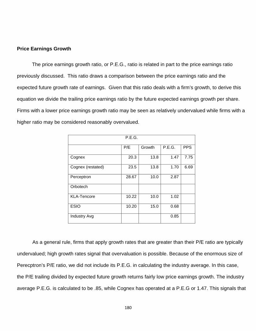
180
Price Earnings Growth
The price earnings growth ratio, or P.E.G., ratio is related in part to the price earnings ratio
previously discussed. This ratio draws a comparison between the price earnings ratio and the
expected future growth rate of earnings. Given that this ratio deals with a firm’s growth, to derive this
equation we divide the trailing price earnings ratio by the future expected earnings growth per share.
Firms with a lower price earnings growth ratio may be seen as relatively undervalued while firms with a
higher ratio may be considered reasonably overvalued.
P.E.G.
P/E Growth P.E.G. PPS
Cognex 20.3 13.8 1.47 7.75
Cognex (restated) 23.5 13.8 1.70 6.69
Perceptron 28.67 10.0 2.87
Orbotech
KLA-Tencore 10.22 10.0 1.02
ESIO 10.20 15.0 0.68
Industry Avg 0.85
As a general rule, firms that apply growth rates that are greater than their P/E ratio are typically
undervalued; high growth rates signal that overvaluation is possible. Because of the enormous size of
Perecptron’s P/E ratio, we did not include its P.E.G. in calculating the industry average. In this case,
the P/E trailing divided by expected future growth returns fairly low price earnings growth. The industry
average P.E.G. is calculated to be .85, while Cognex has operated at a P.E.G or 1.47. This signals that
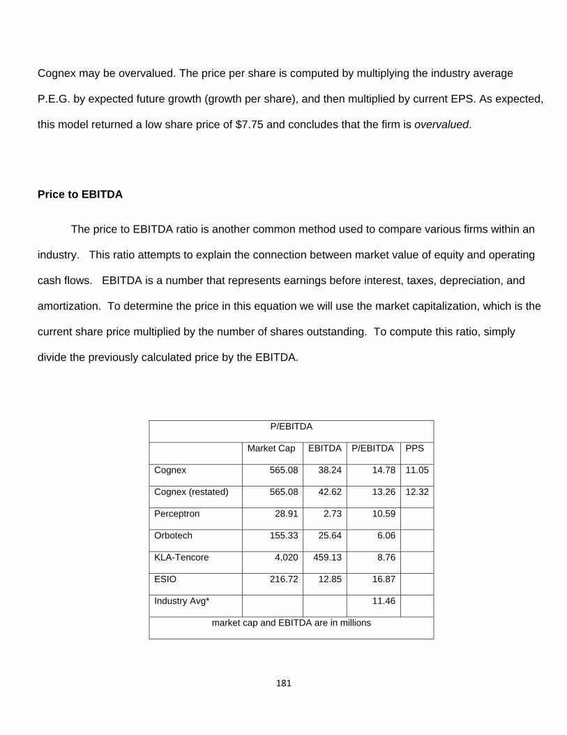
181
Cognex may be overvalued. The price per share is computed by multiplying the industry average
P.E.G. by expected future growth (growth per share), and then multiplied by current EPS. As expected,
this model returned a low share price of $7.75 and concludes that the firm is overvalued.
Price to EBITDA
The price to EBITDA ratio is another common method used to compare various firms within an
industry. This ratio attempts to explain the connection between market value of equity and operating
cash flows. EBITDA is a number that represents earnings before interest, taxes, depreciation, and
amortization. To determine the price in this equation we will use the market capitalization, which is the
current share price multiplied by the number of shares outstanding. To compute this ratio, simply
divide the previously calculated price by the EBITDA.
P/EBITDA
Market Cap EBITDA P/EBITDA PPS
Cognex 565.08 38.24 14.78 11.05
Cognex (restated) 565.08 42.62 13.26 12.32
Perceptron 28.91 2.73 10.59
Orbotech 155.33 25.64 6.06
KLA-Tencore 4,020 459.13 8.76
ESIO 216.72 12.85 16.87
Industry Avg* 11.46
market cap and EBITDA are in millions
182
Data from KLA- Tencor and Perceptron were not used because their market caps just aren’t
comparable with those of Cognex and similar competitors. The healthy EBITDA numbers for Cognex
indicates efficient cash flow operations, which play a vital role in determining value of the firm.
Assessed share price is calculated by multiplying the industry average P/EBITDA by Cognex EBITDA,
and then divided by number of shares outstanding. The original financials indicate that the firm is
overvalued with a model share price of $11.05, %17.5 below the observed share price. The restated
financials returned a share price of %12.32, deviating only 8% from the observed price, indicating a
fairly valued firm.
Enterprise Value to EBITDA
This ratio is a valuable method in the valuation and comparison of firm’s stock prices. The most
important element in using this ratio is that the outcome is completely unaffected by a company’s
capital structure. This ratio is similar to the previously discussed price to earnings method; however,
this technique will allow analysts to value a firm negligent of debt obligations.
To begin this calculation the enterprise value must be determined. To derive the enterprise
value we must add the book value of equity to the market value of equity then deduct cash as well as
the company’s long and short term investments. EBITDA as previously mentioned is representative of
earnings before interest, taxes, depreciation, and amortization. Once these two values have been
established we can calculate the enterprise value to EBITDA ratio. To compute this ratio we will divide
the predetermined enterprise value by EBITDA.
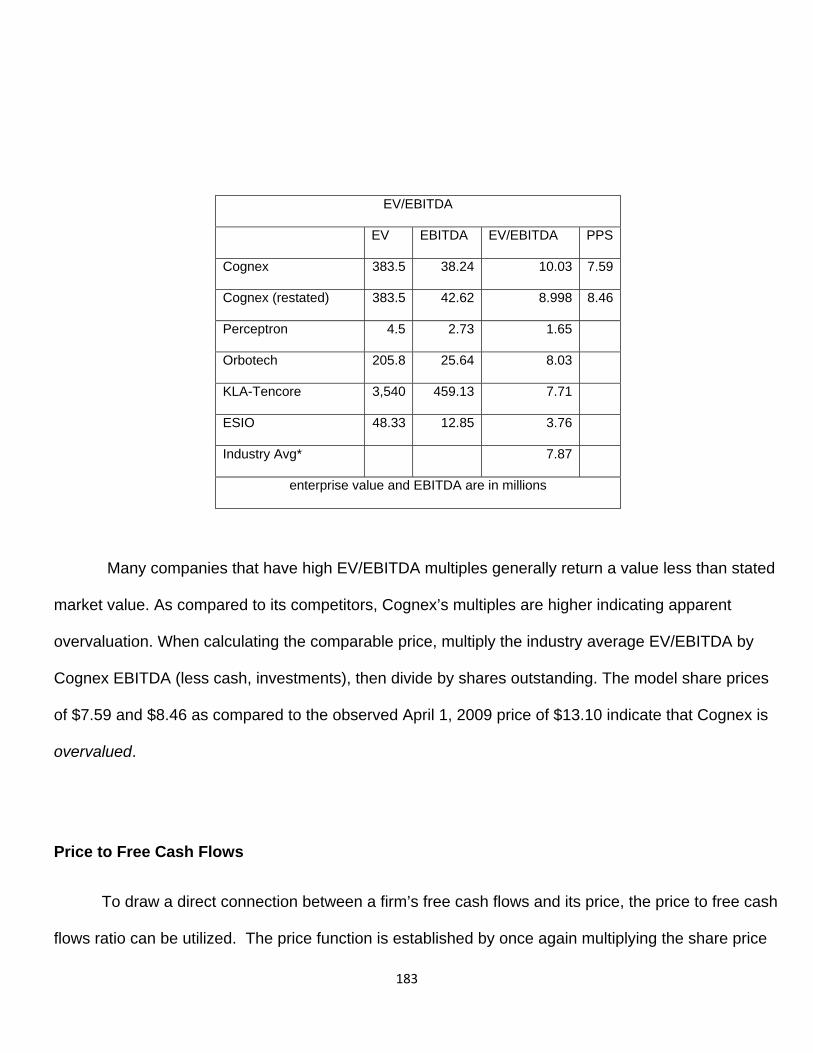
183
EV/EBITDA
EV EBITDA EV/EBITDA PPS
Cognex 383.5 38.24 10.03 7.59
Cognex (restated) 383.5 42.62 8.998 8.46
Perceptron 4.5 2.73 1.65
Orbotech 205.8 25.64 8.03
KLA-Tencore 3,540 459.13 7.71
ESIO 48.33 12.85 3.76
Industry Avg* 7.87
enterprise value and EBITDA are in millions
Many companies that have high EV/EBITDA multiples generally return a value less than stated
market value. As compared to its competitors, Cognex’s multiples are higher indicating apparent
overvaluation. When calculating the comparable price, multiply the industry average EV/EBITDA by
Cognex EBITDA (less cash, investments), then divide by shares outstanding. The model share prices
of $7.59 and $8.46 as compared to the observed April 1, 2009 price of $13.10 indicate that Cognex is
overvalued.
Price to Free Cash Flows
To draw a direct connection between a firm’s free cash flows and its price, the price to free cash
flows ratio can be utilized. The price function is established by once again multiplying the share price
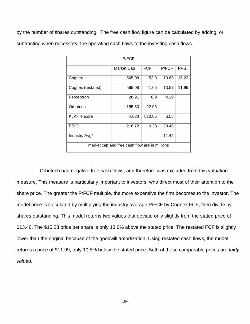
184
by the number of shares outstanding. The free cash flow figure can be calculated by adding, or
subtracting when necessary, the operating cash flows to the investing cash flows.
P/FCF
Market Cap FCF P/FCF PPS
Cognex 565.08 52.9 10.68 15.23
Cognex (restated) 565.08 41.65 13.57 11.99
Perceptron 28.91 6.9 4.19
Orbotech 155.33 -22.06
KLA-Tencore 4,020 610.85 6.58
ESIO 216.72 9.23 23.48
Industry Avg* 11.42
market cap and free cash flow are in millions
Orbotech had negative free cash flows, and therefore was excluded from this valuation
measure. This measure is particularly important to investors, who direct most of their attention to the
share price. The greater the P/FCF multiple, the more expensive the firm becomes to the investor. The
model price is calculated by multiplying the industry average P/FCF by Cognex FCF, then divide by
shares outstanding. This model returns two values that deviate only slightly from the stated price of
$13.40. The $15.23 price per share is only 13.6% above the stated price. The restated FCF is slightly
lower than the original because of the goodwill amortization. Using restated cash flows, the model
returns a price of $11.99, only 10.5% below the stated price. Both of these comparable prices are fairly
valued.
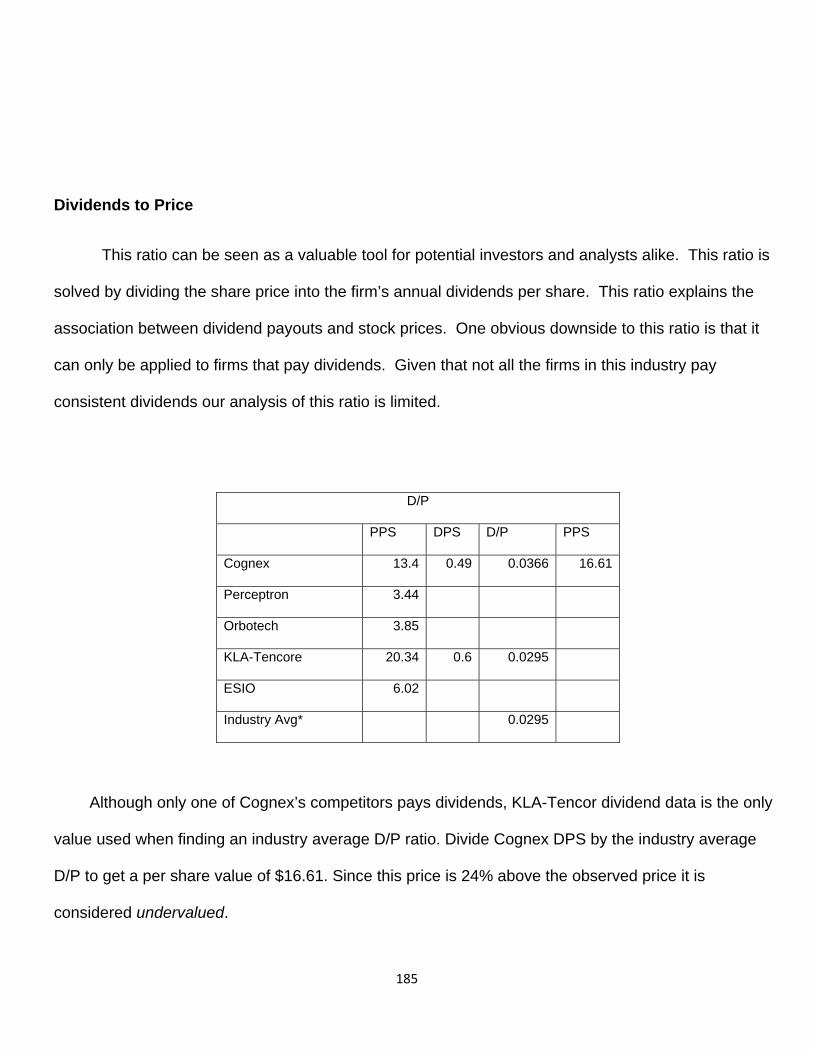
185
Dividends to Price
This ratio can be seen as a valuable tool for potential investors and analysts alike. This ratio is
solved by dividing the share price into the firm’s annual dividends per share. This ratio explains the
association between dividend payouts and stock prices. One obvious downside to this ratio is that it
can only be applied to firms that pay dividends. Given that not all the firms in this industry pay
consistent dividends our analysis of this ratio is limited.
D/P
PPS DPS D/P PPS
Cognex 13.4 0.49 0.0366 16.61
Perceptron 3.44
Orbotech 3.85
KLA-Tencore 20.34 0.6 0.0295
ESIO 6.02
Industry Avg* 0.0295
Although only one of Cognex’s competitors pays dividends, KLA-Tencor dividend data is the only
value used when finding an industry average D/P ratio. Divide Cognex DPS by the industry average
D/P to get a per share value of $16.61. Since this price is 24% above the observed price it is
considered undervalued.
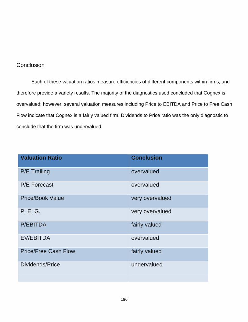
186
Conclusion
Each of these valuation ratios measure efficiencies of different components within firms, and
therefore provide a variety results. The majority of the diagnostics used concluded that Cognex is
overvalued; however, several valuation measures including Price to EBITDA and Price to Free Cash
Flow indicate that Cognex is a fairly valued firm. Dividends to Price ratio was the only diagnostic to
conclude that the firm was undervalued.
Valuation Ratio Conclusion
P/E Trailing overvalued
P/E Forecast overvalued
Price/Book Value very overvalued
P. E. G. very overvalued
P/EBITDA fairly valued
EV/EBITDA overvalued
Price/Free Cash Flow fairly valued
Dividends/Price undervalued
187
Intrinsic Valuation Models
Valuation models are used to estimate the market value price of one share of a company. The
intrinsic valuation models include discounted dividends model, free cash flows model, residual income
model, abnormal earnings growth model, and finally a long run residual income model. Each of these
models provides a different method of estimating the intrinsic value of a firm. They incorporate different
sets of data and use sensitivity analysis to determine accurate valuation estimates. The data used in
these valuation models comes from forecasted data from 2009 through 2018. Both original and
restated income statements, balance sheets, and statements of cash flows are analyzed to provide a
well rounded valuation of our firm.
Discounted Dividends Model
The discounted dividends model is the simplest equity valuation model. Its two main
component drivers are expected future dividends and cost of equity. Our forecast of expected future
earnings was derived from trends in growth rates as well as the dividend payout ratio.
The simplicity and credibility of this model make it popular among analysts; however there are several
weaknesses that should be discussed before you can be completely confident in the sensitivity
analysis. First, the model is extremely sensitive to erratic growth rates, which can adversely affect a
final valuation estimate. Also, because dividend payment is a major driver in this valuation model, firms
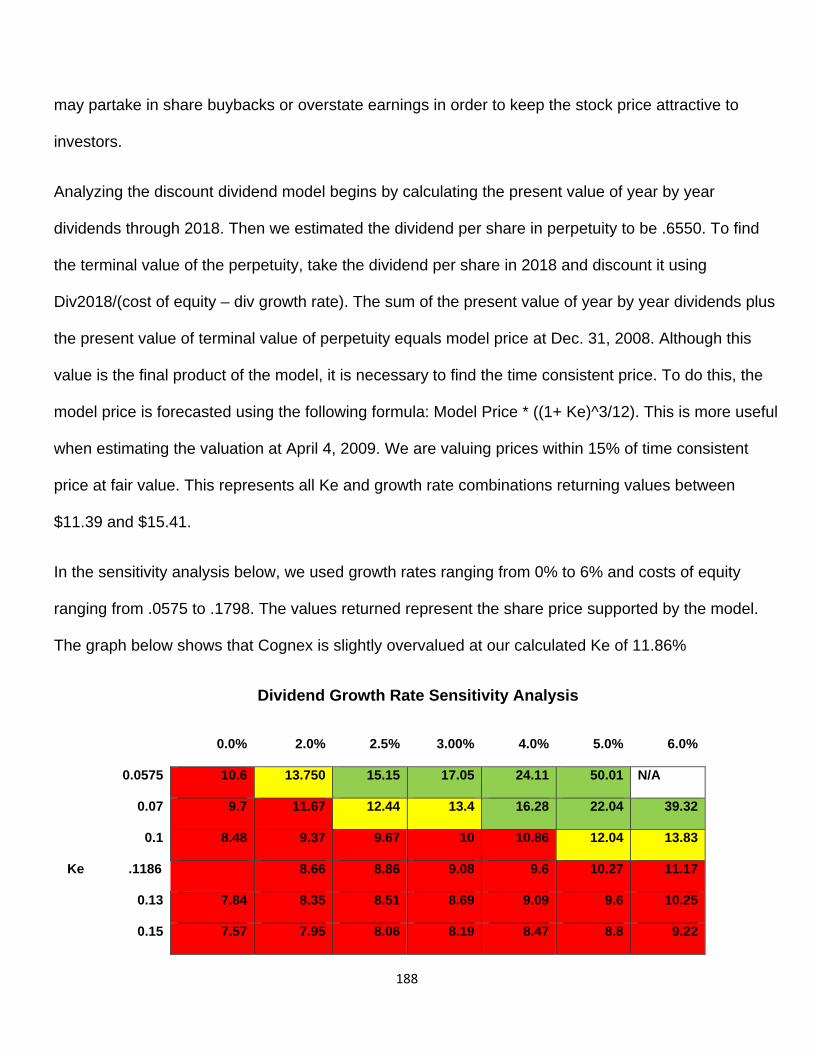
188
may partake in share buybacks or overstate earnings in order to keep the stock price attractive to
investors.
Analyzing the discount dividend model begins by calculating the present value of year by year
dividends through 2018. Then we estimated the dividend per share in perpetuity to be .6550. To find
the terminal value of the perpetuity, take the dividend per share in 2018 and discount it using
Div2018/(cost of equity – div growth rate). The sum of the present value of year by year dividends plus
the present value of terminal value of perpetuity equals model price at Dec. 31, 2008. Although this
value is the final product of the model, it is necessary to find the time consistent price. To do this, the
model price is forecasted using the following formula: Model Price * ((1+ Ke)^3/12). This is more useful
when estimating the valuation at April 4, 2009. We are valuing prices within 15% of time consistent
price at fair value. This represents all Ke and growth rate combinations returning values between
$11.39 and $15.41.
In the sensitivity analysis below, we used growth rates ranging from 0% to 6% and costs of equity
ranging from .0575 to .1798. The values returned represent the share price supported by the model.
The graph below shows that Cognex is slightly overvalued at our calculated Ke of 11.86%
Dividend Growth Rate Sensitivity Analysis
0.0% 2.0% 2.5% 3.00% 4.0% 5.0% 6.0%
0.0575 10.6 13.750 15.15 17.05 24.11 50.01 N/A
0.07 9.7 11.67 12.44 13.4 16.28 22.04 39.32
0.1 8.48 9.37 9.67 10 10.86 12.04 13.83
Ke .1186 8.66 8.86 9.08 9.6 10.27 11.17
0.13 7.84 8.35 8.51 8.69 9.09 9.6 10.25
0.15 7.57 7.95 8.06 8.19 8.47 8.8 9.22
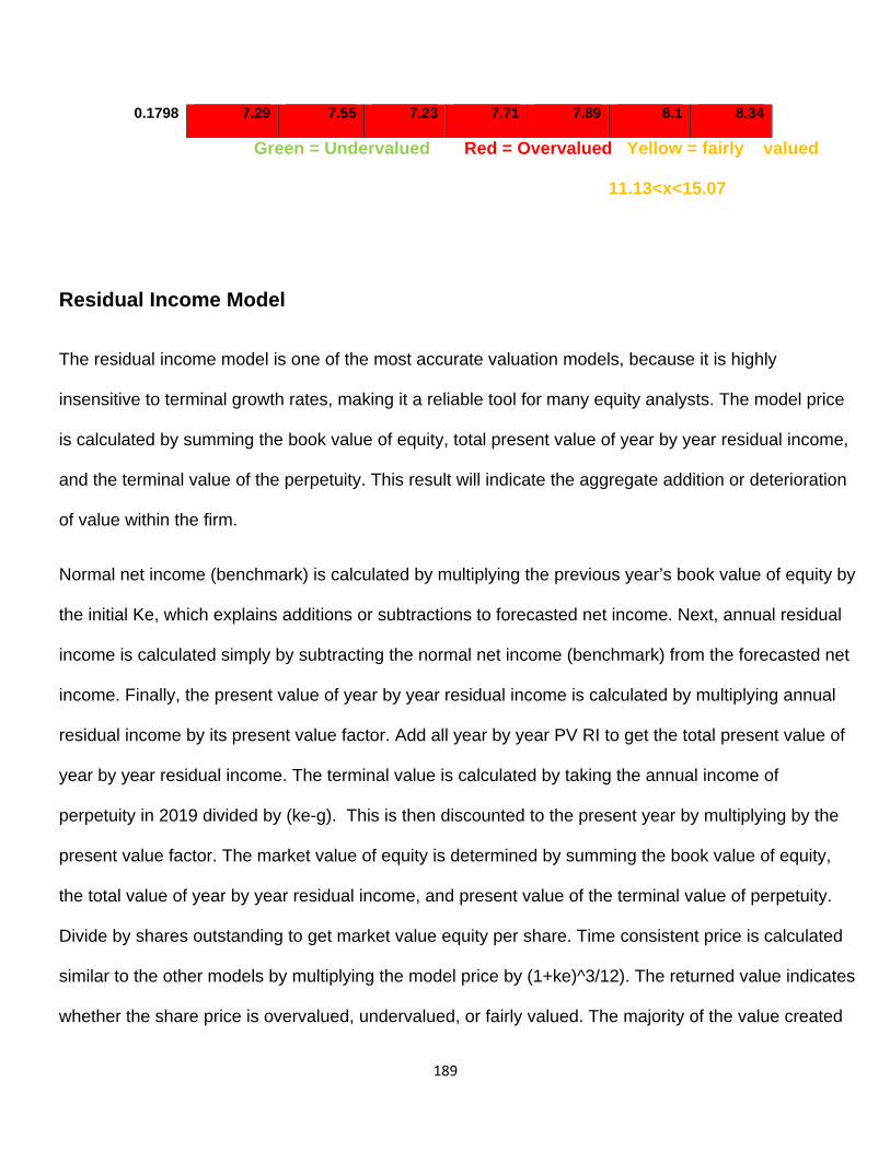
189
0.1798 7.29 7.55 7.23 7.71 7.89 8.1 8.34
Green = Undervalued Red = Overvalued Yellow = fairly valued
11.13<x<15.07
Residual Income Model
The residual income model is one of the most accurate valuation models, because it is highly
insensitive to terminal growth rates, making it a reliable tool for many equity analysts. The model price
is calculated by summing the book value of equity, total present value of year by year residual income,
and the terminal value of the perpetuity. This result will indicate the aggregate addition or deterioration
of value within the firm.
Normal net income (benchmark) is calculated by multiplying the previous year’s book value of equity by
the initial Ke, which explains additions or subtractions to forecasted net income. Next, annual residual
income is calculated simply by subtracting the normal net income (benchmark) from the forecasted net
income. Finally, the present value of year by year residual income is calculated by multiplying annual
residual income by its present value factor. Add all year by year PV RI to get the total present value of
year by year residual income. The terminal value is calculated by taking the annual income of
perpetuity in 2019 divided by (ke-g). This is then discounted to the present year by multiplying by the
present value factor. The market value of equity is determined by summing the book value of equity,
the total value of year by year residual income, and present value of the terminal value of perpetuity.
Divide by shares outstanding to get market value equity per share. Time consistent price is calculated
similar to the other models by multiplying the model price by (1+ke)^3/12). The returned value indicates
whether the share price is overvalued, undervalued, or fairly valued. The majority of the value created
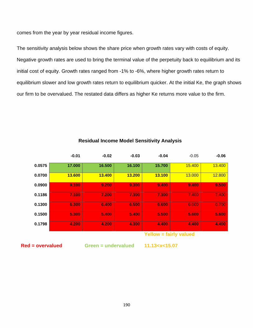
190
comes from the year by year residual income figures.
The sensitivity analysis below shows the share price when growth rates vary with costs of equity.
Negative growth rates are used to bring the terminal value of the perpetuity back to equilibrium and its
initial cost of equity. Growth rates ranged from -1% to -6%, where higher growth rates return to
equilibrium slower and low growth rates return to equilibrium quicker. At the initial Ke, the graph shows
our firm to be overvalued. The restated data differs as higher Ke returns more value to the firm.
Residual Income Model Sensitivity Analysis
-0.01 -0.02 -0.03 -0.04 -0.05 -0.06
0.0575 17.000 16.500 16.100 15.700 15.400 13.400
0.0700 13.600 13.400 13.200 13.100 13.000 12.800
0.0900 9.100 9.200 9.300 9.400 9.400 9.500
0.1186 7.100 7.200 7.300 7.300 7.400 7.400
0.1300 6.300 6.400 6.500 6.600 6.600 6.700
0.1500 5.300 5.400 5.400 5.500 5.600 5.600
0.1798 4.200 4.200 4.300 4.400 4.400 4.400
Red = overvalued Green = undervalued
Yellow = fairly valued
11.13<x<15.07
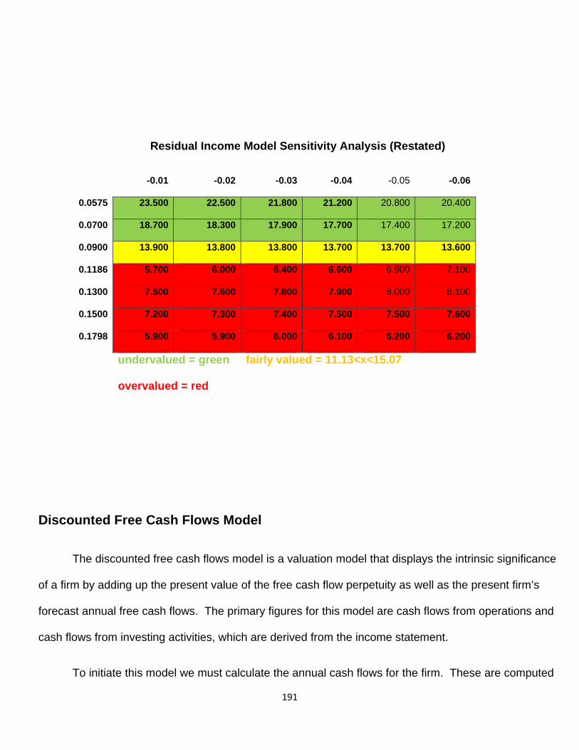
191
Residual Income Model Sensitivity Analysis (Restated)
-0.01 -0.02 -0.03 -0.04 -0.05 -0.06
0.0575 23.500 22.500 21.800 21.200 20.800 20.400
0.0700 18.700 18.300 17.900 17.700 17.400 17.200
0.0900 13.900 13.800 13.800 13.700 13.700 13.600
0.1186 5.700 6.000 6.400 6.600 6.900 7.100
0.1300 7.500 7.600 7.800 7.900 8.000 8.100
0.1500 7.200 7.300 7.400 7.500 7.500 7.600
0.1798 5.900 5.900 6.000 6.100 6.200 6.200
undervalued = green fairly valued = 11.13<x<15.07
overvalued = red
Discounted Free Cash Flows Model
The discounted free cash flows model is a valuation model that displays the intrinsic significance
of a firm by adding up the present value of the free cash flow perpetuity as well as the present firm’s
forecast annual free cash flows. The primary figures for this model are cash flows from operations and
cash flows from investing activities, which are derived from the income statement.
To initiate this model we must calculate the annual cash flows for the firm. These are computed
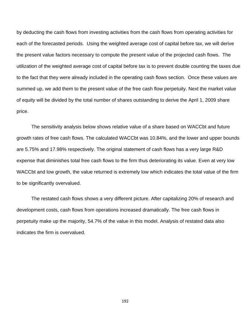
192
by deducting the cash flows from investing activities from the cash flows from operating activities for
each of the forecasted periods. Using the weighted average cost of capital before tax, we will derive
the present value factors necessary to compute the present value of the projected cash flows. The
utilization of the weighted average cost of capital before tax is to prevent double counting the taxes due
to the fact that they were already included in the operating cash flows section. Once these values are
summed up, we add them to the present value of the free cash flow perpetuity. Next the market value
of equity will be divided by the total number of shares outstanding to derive the April 1, 2009 share
price.
The sensitivity analysis below shows relative value of a share based on WACCbt and future
growth rates of free cash flows. The calculated WACCbt was 10.84%, and the lower and upper bounds
are 5.75% and 17.98% respectively. The original statement of cash flows has a very large R&D
expense that diminishes total free cash flows to the firm thus deteriorating its value. Even at very low
WACCbt and low growth, the value returned is extremely low which indicates the total value of the firm
to be significantly overvalued.
The restated cash flows shows a very different picture. After capitalizing 20% of research and
development costs, cash flows from operations increased dramatically. The free cash flows in
perpetuity make up the majority, 54.7% of the value in this model. Analysis of restated data also
indicates the firm is overvalued.
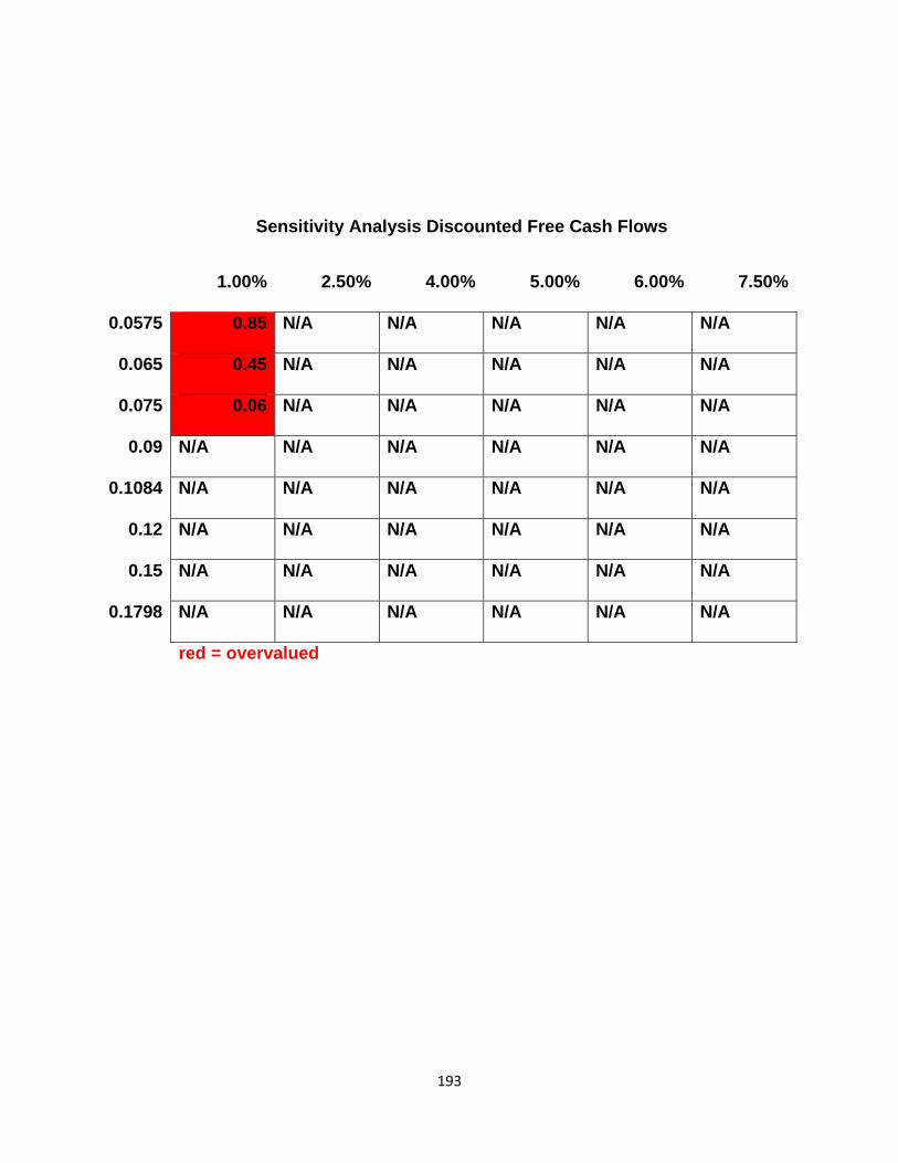
193
Sensitivity Analysis Discounted Free Cash Flows
1.00% 2.50% 4.00% 5.00% 6.00% 7.50%
0.0575 0.85 N/A N/A N/A N/A N/A
0.065 0.45 N/A N/A N/A N/A N/A
0.075 0.06 N/A N/A N/A N/A N/A
0.09 N/A N/A N/A N/A N/A N/A
0.1084 N/A N/A N/A N/A N/A N/A
0.12 N/A N/A N/A N/A N/A N/A
0.15 N/A N/A N/A N/A N/A N/A
0.1798 N/A N/A N/A N/A N/A N/A
red = overvalued
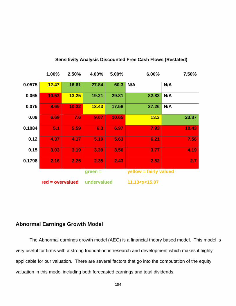
194
Sensitivity Analysis Discounted Free Cash Flows (Restated)
1.00% 2.50% 4.00% 5.00% 6.00% 7.50%
0.0575 12.47 16.61 27.84 60.3 N/A N/A
0.065 10.53 13.25 19.21 29.81 82.83 N/A
0.075 8.65 10.32 13.43 17.58 27.26 N/A
0.09 6.69 7.6 9.07 10.65 13.3 23.87
0.1084 5.1 5.59 6.3 6.97 7.93 10.43
0.12 4.37 4.17 5.19 5.63 6.21 7.56
0.15 3.03 3.19 3.39 3.56 3.77 4.19
0.1798 2.16 2.25 2.35 2.43 2.52 2.7
red = overvalued
green =
undervalued
yellow = fairly valued
11.13<x<15.07
Abnormal Earnings Growth Model
The Abnormal earnings growth model (AEG) is a financial theory based model. This model is
very useful for firms with a strong foundation in research and development which makes it highly
applicable for our valuation. There are several factors that go into the computation of the equity
valuation in this model including both forecasted earnings and total dividends.
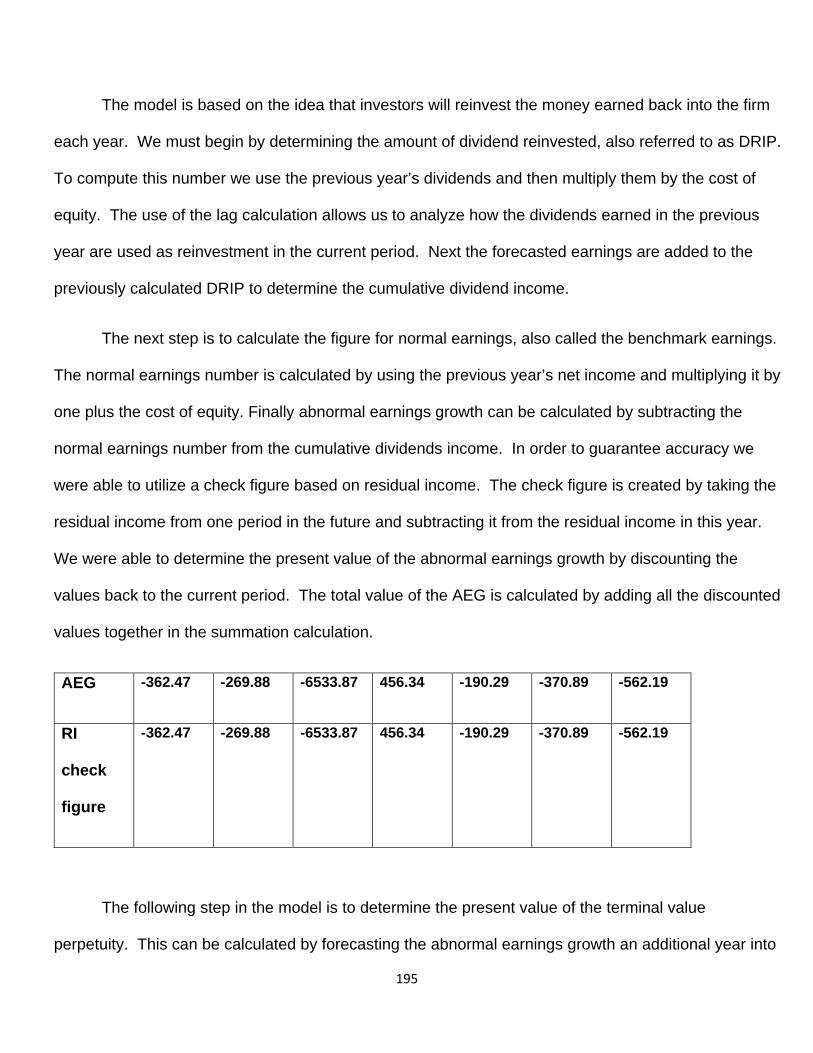
195
The model is based on the idea that investors will reinvest the money earned back into the firm
each year. We must begin by determining the amount of dividend reinvested, also referred to as DRIP.
To compute this number we use the previous year’s dividends and then multiply them by the cost of
equity. The use of the lag calculation allows us to analyze how the dividends earned in the previous
year are used as reinvestment in the current period. Next the forecasted earnings are added to the
previously calculated DRIP to determine the cumulative dividend income.
The next step is to calculate the figure for normal earnings, also called the benchmark earnings.
The normal earnings number is calculated by using the previous year’s net income and multiplying it by
one plus the cost of equity. Finally abnormal earnings growth can be calculated by subtracting the
normal earnings number from the cumulative dividends income. In order to guarantee accuracy we
were able to utilize a check figure based on residual income. The check figure is created by taking the
residual income from one period in the future and subtracting it from the residual income in this year.
We were able to determine the present value of the abnormal earnings growth by discounting the
values back to the current period. The total value of the AEG is calculated by adding all the discounted
values together in the summation calculation.
AEG -362.47 -269.88 -6533.87 456.34 -190.29 -370.89 -562.19
RI
check
figure
-362.47 -269.88 -6533.87 456.34 -190.29 -370.89 -562.19
The following step in the model is to determine the present value of the terminal value
perpetuity. This can be calculated by forecasting the abnormal earnings growth an additional year into
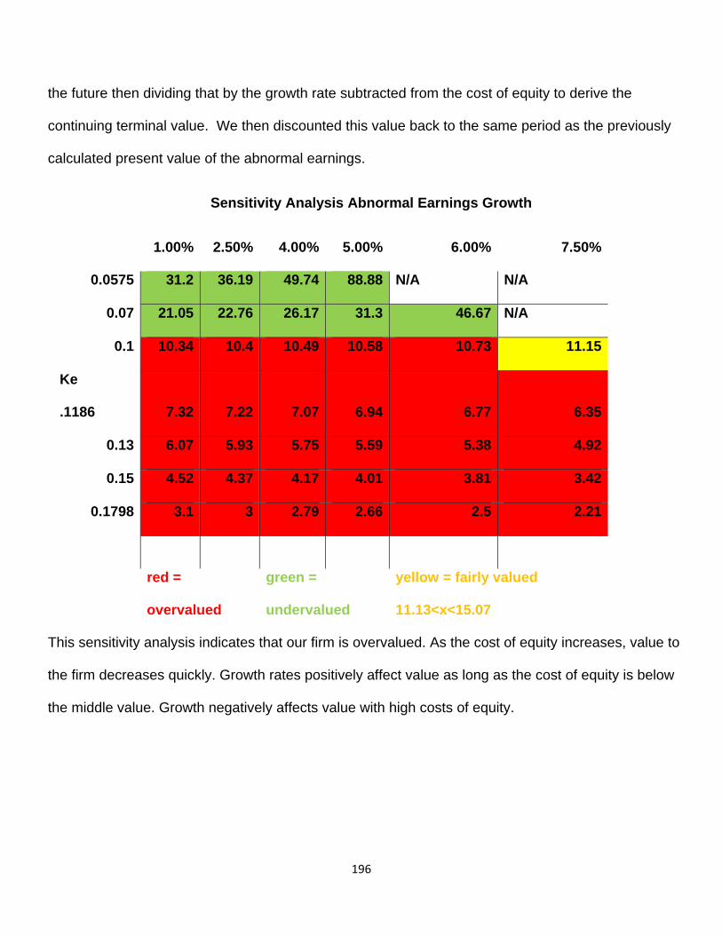
196
the future then dividing that by the growth rate subtracted from the cost of equity to derive the
continuing terminal value. We then discounted this value back to the same period as the previously
calculated present value of the abnormal earnings.
Sensitivity Analysis Abnormal Earnings Growth
1.00% 2.50% 4.00% 5.00% 6.00% 7.50%
0.0575 31.2 36.19 49.74 88.88 N/A N/A
0.07 21.05 22.76 26.17 31.3 46.67 N/A
0.1 10.34 10.4 10.49 10.58 10.73 11.15
Ke
.1186 7.32 7.22 7.07 6.94 6.77 6.35
0.13 6.07 5.93 5.75 5.59 5.38 4.92
0.15 4.52 4.37 4.17 4.01 3.81 3.42
0.1798 3.1 3 2.79 2.66 2.5 2.21
red =
overvalued
green =
undervalued
yellow = fairly valued
11.13<x<15.07
This sensitivity analysis indicates that our firm is overvalued. As the cost of equity increases, value to
the firm decreases quickly. Growth rates positively affect value as long as the cost of equity is below
the middle value. Growth negatively affects value with high costs of equity.
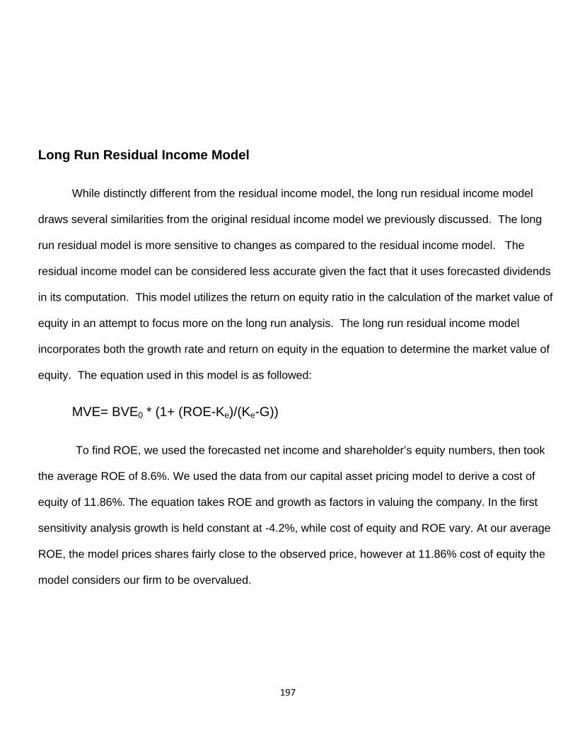
197
Long Run Residual Income Model
While distinctly different from the residual income model, the long run residual income model
draws several similarities from the original residual income model we previously discussed. The long
run residual model is more sensitive to changes as compared to the residual income model. The
residual income model can be considered less accurate given the fact that it uses forecasted dividends
in its computation. This model utilizes the return on equity ratio in the calculation of the market value of
equity in an attempt to focus more on the long run analysis. The long run residual income model
incorporates both the growth rate and return on equity in the equation to determine the market value of
equity. The equation used in this model is as followed:
MVE= BVE0 * (1+ (ROE-Ke)/(Ke-G))
To find ROE, we used the forecasted net income and shareholder’s equity numbers, then took
the average ROE of 8.6%. We used the data from our capital asset pricing model to derive a cost of
equity of 11.86%. The equation takes ROE and growth as factors in valuing the company. In the first
sensitivity analysis growth is held constant at -4.2%, while cost of equity and ROE vary. At our average
ROE, the model prices shares fairly close to the observed price, however at 11.86% cost of equity the
model considers our firm to be overvalued.
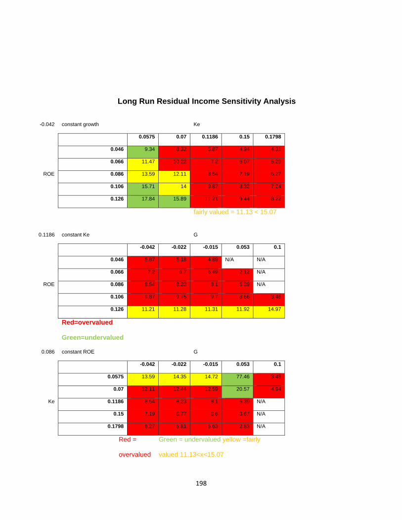
198
Long Run Residual Income Sensitivity Analysis
-0.042 constant growth Ke
0.0575 0.07 0.1186 0.15 0.1798
0.046 9.34 8.32 5.87 4.94 4.31
0.066 11.47 10.22 7.2 6.07 5.29
ROE 0.086 13.59 12.11 8.54 7.19 6.27
0.106 15.71 14 9.87 8.32 7.24
0.126 17.84 15.89 11.21 9.44 8.22
fairly valued = 11.13 < 15.07
0.1186 constant Ke G
-0.042 -0.022 -0.015 0.053 0.1
0.046 5.87 5.18 4.89 N/A N/A
0.066 7.2 6.7 6.49 2.12 N/A
ROE 0.086 8.54 8.23 8.1 5.39 N/A
0.106 9.87 9.75 9.7 8.66 3.46
0.126 11.21 11.28 11.31 11.92 14.97
Red=overvalued
Green=undervalued
0.086 constant ROE G
-0.042 -0.022 -0.015 0.053 0.1
0.0575 13.59 14.35 14.72 77.46 3.48
0.07 12.11 12.44 12.59 20.57 4.94
Ke 0.1186 8.54 8.23 8.1 5.39 N/A
0.15 7.19 6.77 6.6 3.67 N/A
0.1798 6.27 5.81 5.63 2.83 N/A
Red =
overvalued
Green = undervalued yellow =fairly
valued 11.13<x<15.07
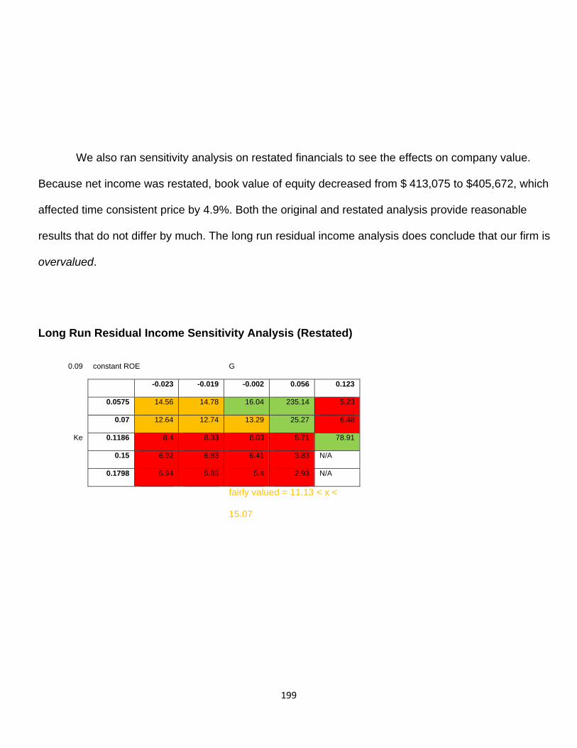
199
We also ran sensitivity analysis on restated financials to see the effects on company value.
Because net income was restated, book value of equity decreased from $ 413,075 to $405,672, which
affected time consistent price by 4.9%. Both the original and restated analysis provide reasonable
results that do not differ by much. The long run residual income analysis does conclude that our firm is
overvalued.
Long Run Residual Income Sensitivity Analysis (Restated)
0.09 constant ROE G
-0.023 -0.019 -0.002 0.056 0.123
0.0575 14.56 14.78 16.04 235.14 5.23
0.07 12.64 12.74 13.29 25.27 6.48
Ke 0.1186 8.4 8.33 8.03 5.71 78.91
0.15 6.92 6.83 6.41 3.83 N/A
0.1798 5.94 5.85 5.4 2.93 N/A
fairly valued = 11.13 < x <
15.07
200
Analyst Recommendation
We have concluded a thorough and in-depth analysis of Cognex and its competitors to make a
solid assessment of the true value of the company. Our analysis has led us to believe that Cognex is
overvalued. Many unique characteristics of Cognex’s business operations and industry data were used
to determine the appropriate appraisal. Key accounting policies, financial statements and industry
trends all provided information regarding value. Through analysis of these topics, specific line items
were forecasted out in order to give a credible picture of where Cognex will stand in the next 10 years,
through 2018. The forecasted data was incorporated into several intrinsic valuation models to value
shares of the company. The results of these models indicate that although Cognex is a profitable firm,
it is not worth the current market price.
Industry analysis is a vital part in valuing a firm. It is important to get a picture of industry trends
as a whole in order to assess value of a specific firm in that industry. Cognex operates in Scientific and
Technical Instruments industry; we have identified three companies close to Cognex that help
determine appropriate value. KLA-Tencor, ESIO, and Orbotech operate with similar business strategy.
These companies invest heavily in research and development, sales strategies involves superior
product quality and product differentiation, as well as investing heavily in brand image. Studying these
industry qualities all helped to gain a true picture of company value.
After industry analysis, we studied the accounting policies the company uses and the amount of
disclosure in the company 10-K. Key accounting policies for Cognex were research and development,
goodwill, and foreign currency. We examined accounts relating to the key accounting policies to ensure
decision making by managers was credible. We looked for areas of the financial statements that may
have red flags and finally worked to undo the accounting distortions. In evaluating these policies we
201
determined that research and development and goodwill presented red flags. It was found that there
was not sufficient disclosure in the R&D and goodwill accounts. Research and development expenses
were extremely high and the goodwill recorded was very high as well, distorting the balance sheet. We
computed a hypothetical amortization of goodwill at 20% and capitalized 20% of R&D expenses to help
see the value within the firm.
In assessing financial performance of Cognex, a series of ratios were analyzed to find
performance of specific sectors of the business. These ratios are separated into liquidity, profitability
and capital structure. Averages of these ratios were used to see how Cognex compared directly with
firms in its industry. It was determined that Cognex consistently performs at or above the industry
average.
The final step in the equity valuation analysis integrates a variety of valuation techniques to find
intrinsic value of Cognex. These techniques included computing comparables along with several
intrinsic valuation models. The comparables model is an effective method of evaluation, but it only
takes industry averages into account. Intrinsic valuation models provide a more accurate means of
assessing data, but incorporate analyst estimates which may not always be precise.
In the method of comparables, most of the diagnostics returned overvalued conclusions.
P/EBITDA and Price/Free Cash Flow concluded fair value, while the only diagnostic to conclude
undervalued was Dividends/Price. The valuation models also determined that Cognex was overvalued.
Each model examines a unique part of the business and provides a value based on the specific
performance factors. We determined that the residual income model provided the least amount of
information, as it was the least affected by terminal values and growth rates.
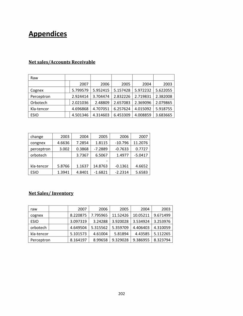
202
Appendices
Net sales/Accounts Receivable
Raw 2007 2006 2005 2004 2003
Cognex 5.799579 5.952415 5.157428 5.972232 5.622055 Perceptron 2.924414 3.704474 2.832226 2.719831 2.382008 Orbotech 2.021036 2.48809 2.657083 2.369096 2.079865 Kla‐tencor 4.696868 4.707051 6.257624 4.015092 5.918755 ESIO 4.501346 4.314603 6.453309 4.008859 3.683665
change 2003 2004 2005 2006 2007congnex 4.6636 7.2854 1.8115 ‐10.796 11.2076perceptron 3.002 0.3868 ‐7.2889 ‐0.7633 0.7727orbotech 3.7367 6.5067 1.4977 ‐5.0417
kla‐tencor 5.8766 1.1637 ‐
14.8763 ‐0.1361 4.6652ESIO 1.3941 4.8401 ‐1.6821 ‐2.2314 5.6583
Net Sales/ Inventory
raw 2007 2006 2005 2004 2003cognex 8.220875 7.795965 11.52426 10.05211 9.671499ESIO 3.097319 3.24288 3.920028 3.534924 3.253976orbotech 4.649504 5.315562 5.359709 4.406403 4.310059kla‐tencor 5.101573 4.61004 5.81894 4.43585 5.112265Perceptron 8.164197 8.99658 9.329028 9.386955 8.323794
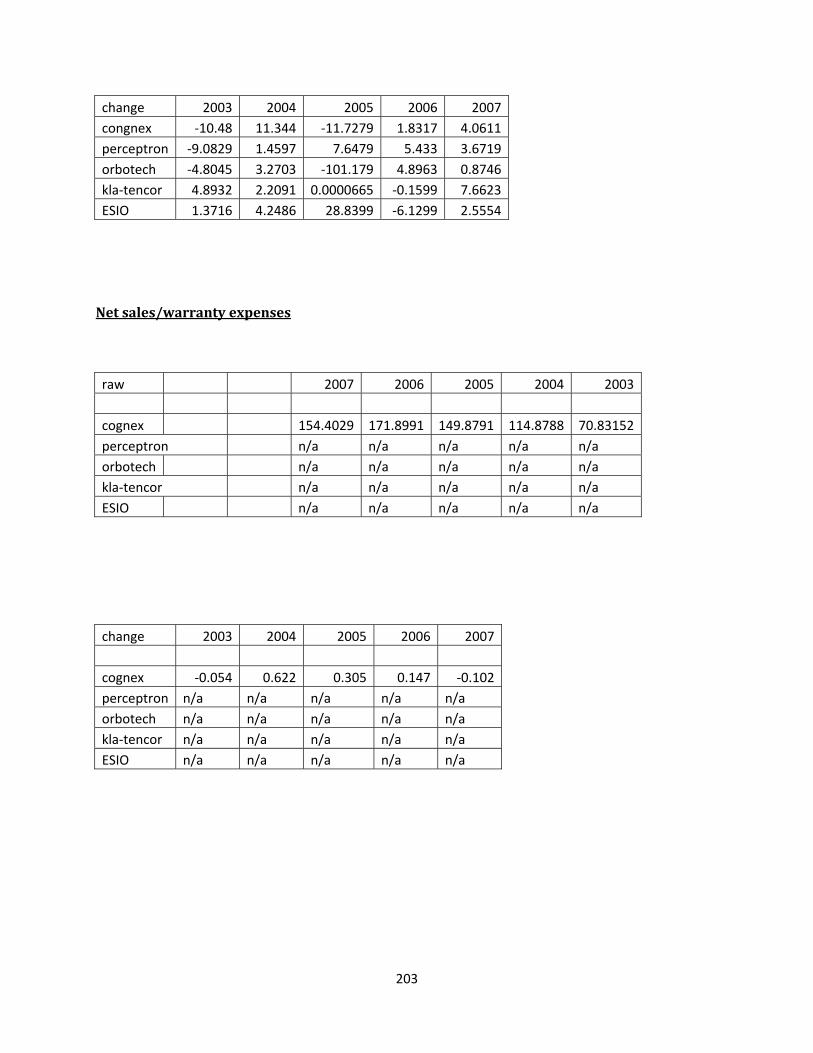
203
change 2003 2004 2005 2006 2007congnex ‐10.48 11.344 ‐11.7279 1.8317 4.0611perceptron ‐9.0829 1.4597 7.6479 5.433 3.6719orbotech ‐4.8045 3.2703 ‐101.179 4.8963 0.8746kla‐tencor 4.8932 2.2091 0.0000665 ‐0.1599 7.6623ESIO 1.3716 4.2486 28.8399 ‐6.1299 2.5554
Net sales/warranty expenses
raw 2007 2006 2005 2004 2003
cognex 154.4029 171.8991 149.8791 114.8788 70.83152 perceptron n/a n/a n/a n/a n/a orbotech n/a n/a n/a n/a n/a kla‐tencor n/a n/a n/a n/a n/a ESIO n/a n/a n/a n/a n/a
change 2003 2004 2005 2006 2007
cognex ‐0.054 0.622 0.305 0.147 ‐0.102perceptron n/a n/a n/a n/a n/a orbotech n/a n/a n/a n/a n/a kla‐tencor n/a n/a n/a n/a n/a ESIO n/a n/a n/a n/a n/a
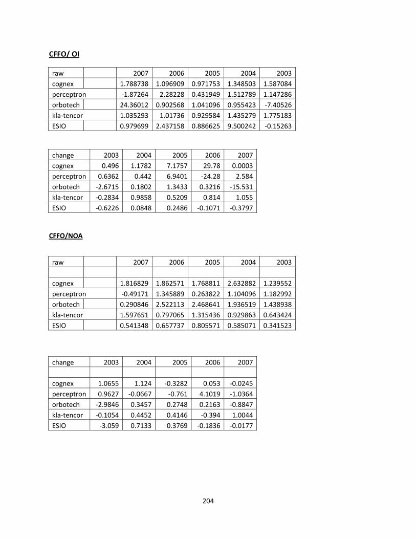
204
CFFO/ OI
raw 2007 2006 2005 2004 2003cognex 1.788738 1.096909 0.971753 1.348503 1.587084perceptron ‐1.87264 2.28228 0.431949 1.512789 1.147286orbotech 24.36012 0.902568 1.041096 0.955423 ‐7.40526kla‐tencor 1.035293 1.01736 0.929584 1.435279 1.775183ESIO 0.979699 2.437158 0.886625 9.500242 ‐0.15263
change 2003 2004 2005 2006 2007cognex 0.496 1.1782 7.1757 29.78 0.0003perceptron 0.6362 0.442 6.9401 ‐24.28 2.584orbotech ‐2.6715 0.1802 1.3433 0.3216 ‐15.531kla‐tencor ‐0.2834 0.9858 0.5209 0.814 1.055ESIO ‐0.6226 0.0848 0.2486 ‐0.1071 ‐0.3797
CFFO/NOA
raw 2007 2006 2005 2004 2003
cognex 1.816829 1.862571 1.768811 2.632882 1.239552perceptron ‐0.49171 1.345889 0.263822 1.104096 1.182992orbotech 0.290846 2.522113 2.468641 1.936519 1.438938kla‐tencor 1.597651 0.797065 1.315436 0.929863 0.643424ESIO 0.541348 0.657737 0.805571 0.585071 0.341523
change 2003 2004 2005 2006 2007
cognex 1.0655 1.124 ‐0.3282 0.053 ‐0.0245perceptron 0.9627 ‐0.0667 ‐0.761 4.1019 ‐1.0364orbotech ‐2.9846 0.3457 0.2748 0.2163 ‐0.8847kla‐tencor ‐0.1054 0.4452 0.4146 ‐0.394 1.0044ESIO ‐3.059 0.7133 0.3769 ‐0.1836 ‐0.0177
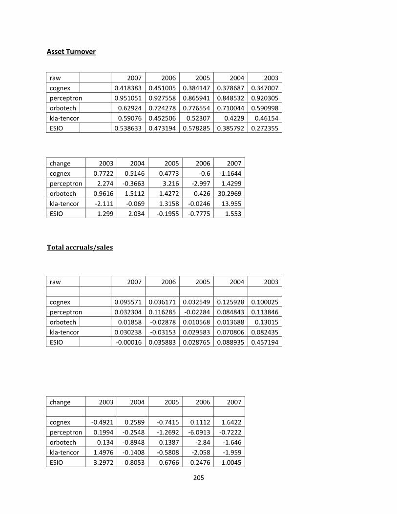
205
Asset Turnover
raw 2007 2006 2005 2004 2003cognex 0.418383 0.451005 0.384147 0.378687 0.347007perceptron 0.951051 0.927558 0.865941 0.848532 0.920305orbotech 0.62924 0.724278 0.776554 0.710044 0.590998kla‐tencor 0.59076 0.452506 0.52307 0.4229 0.46154ESIO 0.538633 0.473194 0.578285 0.385792 0.272355
change 2003 2004 2005 2006 2007cognex 0.7722 0.5146 0.4773 ‐0.6 ‐1.1644perceptron 2.274 ‐0.3663 3.216 ‐2.997 1.4299orbotech 0.9616 1.5112 1.4272 0.426 30.2969kla‐tencor ‐2.111 ‐0.069 1.3158 ‐0.0246 13.955ESIO 1.299 2.034 ‐0.1955 ‐0.7775 1.553
Total accruals/sales
raw 2007 2006 2005 2004 2003
cognex 0.095571 0.036171 0.032549 0.125928 0.100025perceptron 0.032304 0.116285 ‐0.02284 0.084843 0.113846orbotech 0.01858 ‐0.02878 0.010568 0.013688 0.13015kla‐tencor 0.030238 ‐0.03153 0.029583 0.070806 0.082435ESIO ‐0.00016 0.035883 0.028765 0.088935 0.457194
change 2003 2004 2005 2006 2007
cognex ‐0.4921 0.2589 ‐0.7415 0.1112 1.6422perceptron 0.1994 ‐0.2548 ‐1.2692 ‐6.0913 ‐0.7222orbotech 0.134 ‐0.8948 0.1387 ‐2.84 ‐1.646kla‐tencor 1.4976 ‐0.1408 ‐0.5808 ‐2.058 ‐1.959ESIO 3.2972 ‐0.8053 ‐0.6766 0.2476 ‐1.0045
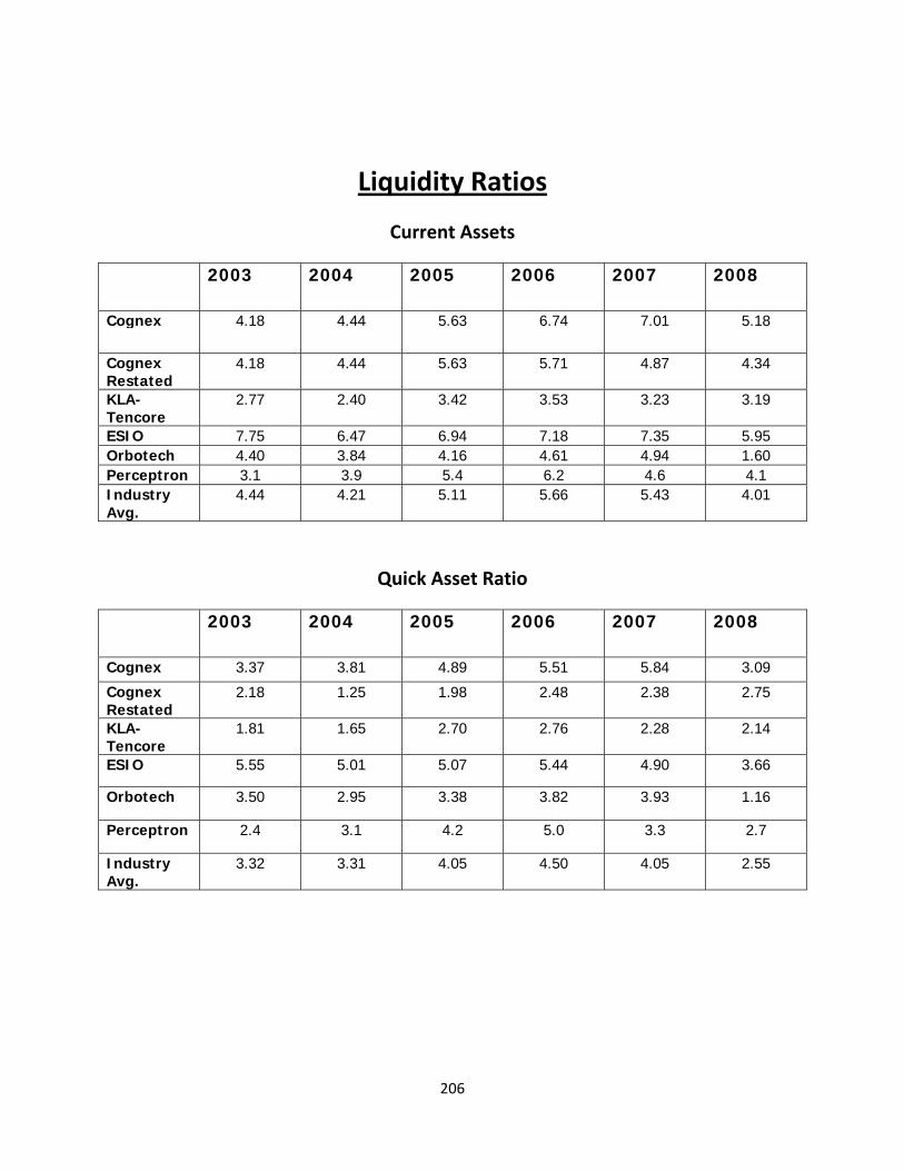
206
Liquidity Ratios
Current Assets
2003 2004 2005 2006 2007 2008
Cognex 4.18 4.44 5.63 6.74 7.01 5.18
Cognex Restated
4.18 4.44 5.63 5.71 4.87 4.34
KLA-Tencore
2.77 2.40 3.42 3.53 3.23 3.19
ESIO 7.75 6.47 6.94 7.18 7.35 5.95 Orbotech 4.40 3.84 4.16 4.61 4.94 1.60 Perceptron 3.1 3.9 5.4 6.2 4.6 4.1 Industry Avg.
4.44 4.21 5.11 5.66 5.43 4.01
Quick Asset Ratio
2003 2004 2005 2006 2007 2008
Cognex 3.37 3.81 4.89 5.51 5.84 3.09
Cognex Restated
2.18 1.25 1.98 2.48 2.38 2.75
KLA-Tencore
1.81 1.65 2.70 2.76 2.28 2.14
ESIO 5.55 5.01 5.07 5.44 4.90 3.66
Orbotech 3.50 2.95 3.38 3.82 3.93 1.16
Perceptron 2.4 3.1 4.2 5.0 3.3 2.7
Industry Avg.
3.32 3.31 4.05 4.50 4.05 2.55
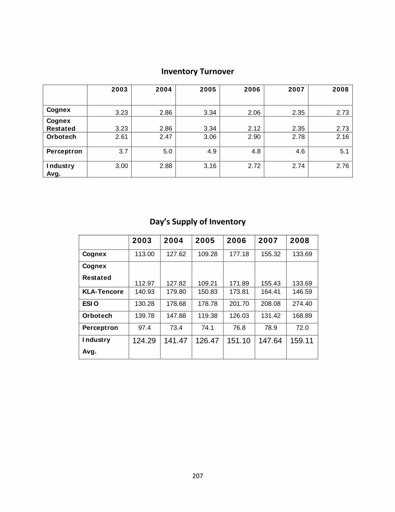
207
Inventory Turnover
2003 2004 2005 2006 2007 2008
Cognex 3.23 2.86 3.34 2.06 2.35 2.73Cognex Restated 3.23 2.86 3.34 2.12 2.35 2.73Orbotech 2.61 2.47 3.06 2.90 2.78 2.16
Perceptron 3.7 5.0 4.9 4.8 4.6 5.1
Industry Avg.
3.00 2.88 3.16 2.72 2.74 2.76
Day’s Supply of Inventory
2003 2004 2005 2006 2007 2008
Cognex 113.00 127.62 109.28 177.18 155.32 133.69
Cognex
Restated 112.97 127.82 109.21 171.89 155.43 133.69
KLA-Tencore 140.93 179.80 150.83 173.81 164.41 146.59
ESIO 130.28 178.68 178.78 201.70 208.08 274.40
Orbotech 139.78 147.88 119.38 126.03 131.42 168.89
Perceptron 97.4 73.4 74.1 76.8 78.9 72.0
Industry
Avg.
124.29 141.47 126.47 151.10 147.64 159.11
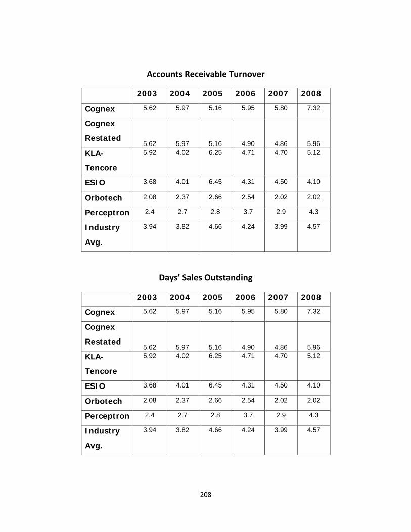
208
Accounts Receivable Turnover
2003 2004 2005 2006 2007 2008
Cognex 5.62 5.97 5.16 5.95 5.80 7.32
Cognex
Restated 5.62 5.97 5.16 4.90 4.86 5.96
KLA-
Tencore
5.92 4.02 6.25 4.71 4.70 5.12
ESIO 3.68 4.01 6.45 4.31 4.50 4.10
Orbotech 2.08 2.37 2.66 2.54 2.02 2.02
Perceptron 2.4 2.7 2.8 3.7 2.9 4.3
Industry
Avg.
3.94 3.82 4.66 4.24 3.99 4.57
Days’ Sales Outstanding
2003 2004 2005 2006 2007 2008
Cognex 5.62 5.97 5.16 5.95 5.80 7.32
Cognex
Restated 5.62 5.97 5.16 4.90 4.86 5.96
KLA-
Tencore
5.92 4.02 6.25 4.71 4.70 5.12
ESIO 3.68 4.01 6.45 4.31 4.50 4.10
Orbotech 2.08 2.37 2.66 2.54 2.02 2.02
Perceptron 2.4 2.7 2.8 3.7 2.9 4.3
Industry
Avg.
3.94 3.82 4.66 4.24 3.99 4.57
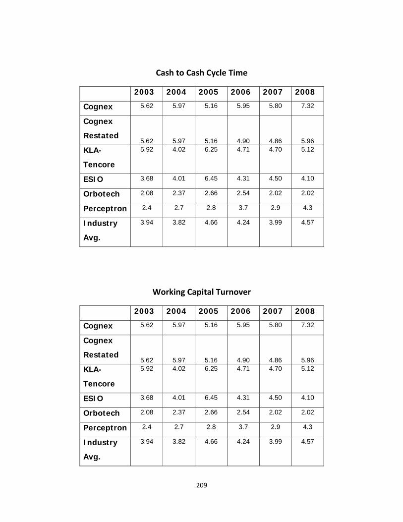
209
Cash to Cash Cycle Time
2003 2004 2005 2006 2007 2008
Cognex 5.62 5.97 5.16 5.95 5.80 7.32
Cognex
Restated 5.62 5.97 5.16 4.90 4.86 5.96
KLA-
Tencore
5.92 4.02 6.25 4.71 4.70 5.12
ESIO 3.68 4.01 6.45 4.31 4.50 4.10
Orbotech 2.08 2.37 2.66 2.54 2.02 2.02
Perceptron 2.4 2.7 2.8 3.7 2.9 4.3
Industry
Avg.
3.94 3.82 4.66 4.24 3.99 4.57
Working Capital Turnover
2003 2004 2005 2006 2007 2008
Cognex 5.62 5.97 5.16 5.95 5.80 7.32
Cognex
Restated 5.62 5.97 5.16 4.90 4.86 5.96
KLA-
Tencore
5.92 4.02 6.25 4.71 4.70 5.12
ESIO 3.68 4.01 6.45 4.31 4.50 4.10
Orbotech 2.08 2.37 2.66 2.54 2.02 2.02
Perceptron 2.4 2.7 2.8 3.7 2.9 4.3
Industry
Avg.
3.94 3.82 4.66 4.24 3.99 4.57
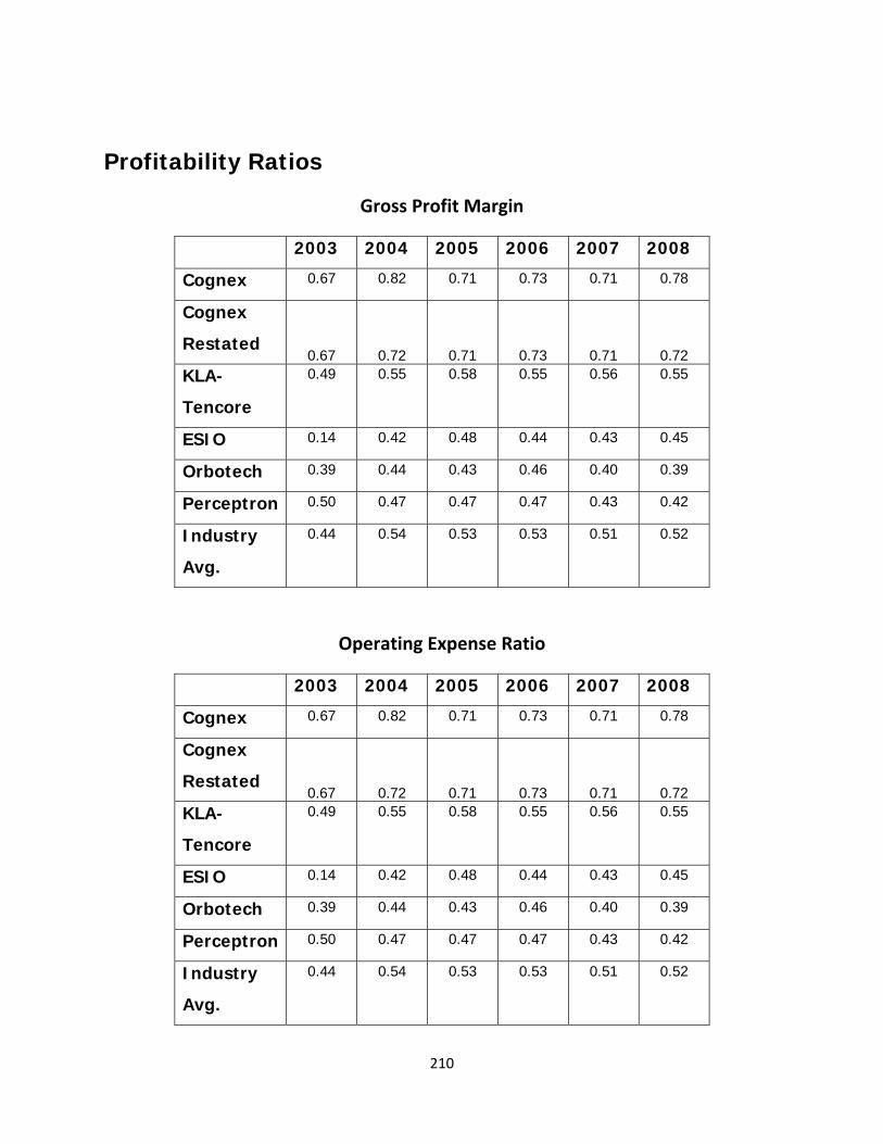
210
Profitability Ratios
Gross Profit Margin
2003 2004 2005 2006 2007 2008
Cognex 0.67 0.82 0.71 0.73 0.71 0.78
Cognex
Restated 0.67 0.72 0.71 0.73 0.71 0.72
KLA-
Tencore
0.49 0.55 0.58 0.55 0.56 0.55
ESIO 0.14 0.42 0.48 0.44 0.43 0.45
Orbotech 0.39 0.44 0.43 0.46 0.40 0.39
Perceptron 0.50 0.47 0.47 0.47 0.43 0.42
Industry
Avg.
0.44 0.54 0.53 0.53 0.51 0.52
Operating Expense Ratio
2003 2004 2005 2006 2007 2008
Cognex 0.67 0.82 0.71 0.73 0.71 0.78
Cognex
Restated 0.67 0.72 0.71 0.73 0.71 0.72
KLA-
Tencore
0.49 0.55 0.58 0.55 0.56 0.55
ESIO 0.14 0.42 0.48 0.44 0.43 0.45
Orbotech 0.39 0.44 0.43 0.46 0.40 0.39
Perceptron 0.50 0.47 0.47 0.47 0.43 0.42
Industry
Avg.
0.44 0.54 0.53 0.53 0.51 0.52
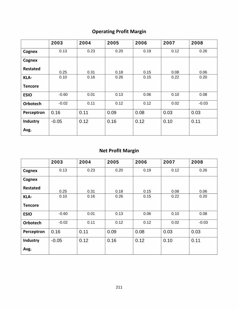
211
Operating Profit Margin
2003 2004 2005 2006 2007 2008
Cognex 0.13 0.23 0.20 0.19 0.12 0.26
Cognex
Restated 0.25 0.31 0.18 0.15 0.08 0.06
KLA‐
Tencore
0.10 0.16 0.26 0.15 0.22 0.20
ESIO -0.60 0.01 0.13 0.06 0.10 0.08
Orbotech -0.02 0.11 0.12 0.12 0.02 -0.03
Perceptron 0.16 0.11 0.09 0.08 0.03 0.03
Industry
Avg.
-0.05 0.12 0.16 0.12 0.10 0.11
Net Profit Margin
2003 2004 2005 2006 2007 2008
Cognex 0.13 0.23 0.20 0.19 0.12 0.26
Cognex
Restated 0.25 0.31 0.18 0.15 0.08 0.06
KLA‐
Tencore
0.10 0.16 0.26 0.15 0.22 0.20
ESIO -0.60 0.01 0.13 0.06 0.10 0.08
Orbotech -0.02 0.11 0.12 0.12 0.02 -0.03
Perceptron 0.16 0.11 0.09 0.08 0.03 0.03
Industry
Avg.
-0.05 0.12 0.16 0.12 0.10 0.11
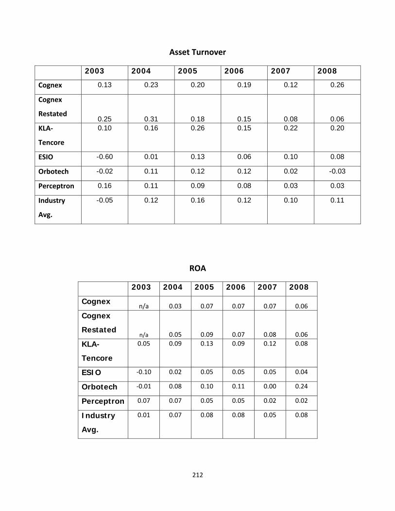
212
Asset Turnover
2003 2004 2005 2006 2007 2008
Cognex 0.13 0.23 0.20 0.19 0.12 0.26
Cognex
Restated 0.25 0.31 0.18 0.15 0.08 0.06
KLA‐
Tencore
0.10 0.16 0.26 0.15 0.22 0.20
ESIO -0.60 0.01 0.13 0.06 0.10 0.08
Orbotech -0.02 0.11 0.12 0.12 0.02 -0.03
Perceptron 0.16 0.11 0.09 0.08 0.03 0.03
Industry
Avg.
-0.05 0.12 0.16 0.12 0.10 0.11
ROA
2003 2004 2005 2006 2007 2008
Cognex n/a 0.03 0.07 0.07 0.07 0.06
Cognex
Restated n/a 0.05 0.09 0.07 0.08 0.06
KLA-
Tencore
0.05 0.09 0.13 0.09 0.12 0.08
ESIO ‐0.10 0.02 0.05 0.05 0.05 0.04
Orbotech ‐0.01 0.08 0.10 0.11 0.00 0.24
Perceptron 0.07 0.07 0.05 0.05 0.02 0.02
Industry
Avg.
0.01 0.07 0.08 0.08 0.05 0.08
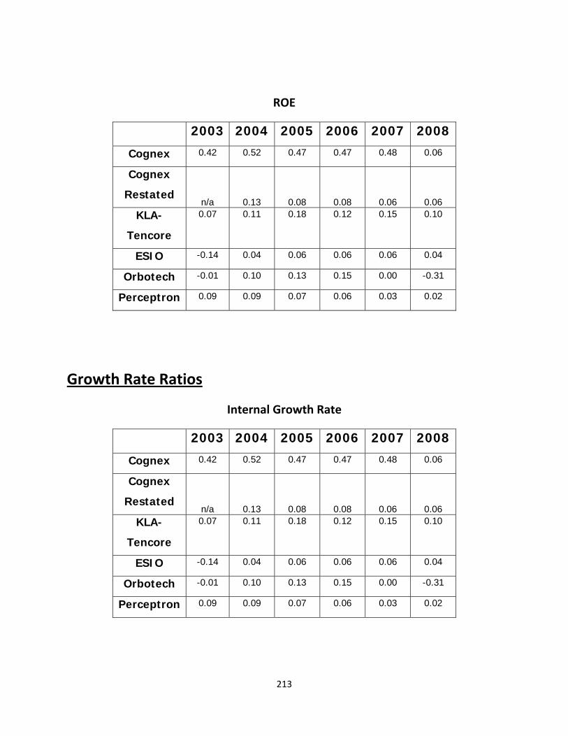
213
ROE
2003 2004 2005 2006 2007 2008
Cognex 0.42 0.52 0.47 0.47 0.48 0.06
Cognex
Restated n/a 0.13 0.08 0.08 0.06 0.06
KLA-
Tencore
0.07 0.11 0.18 0.12 0.15 0.10
ESIO -0.14 0.04 0.06 0.06 0.06 0.04
Orbotech -0.01 0.10 0.13 0.15 0.00 -0.31
Perceptron 0.09 0.09 0.07 0.06 0.03 0.02
Growth Rate Ratios
Internal Growth Rate
2003 2004 2005 2006 2007 2008
Cognex 0.42 0.52 0.47 0.47 0.48 0.06
Cognex
Restated n/a 0.13 0.08 0.08 0.06 0.06
KLA-
Tencore
0.07 0.11 0.18 0.12 0.15 0.10
ESIO -0.14 0.04 0.06 0.06 0.06 0.04
Orbotech -0.01 0.10 0.13 0.15 0.00 -0.31
Perceptron 0.09 0.09 0.07 0.06 0.03 0.02
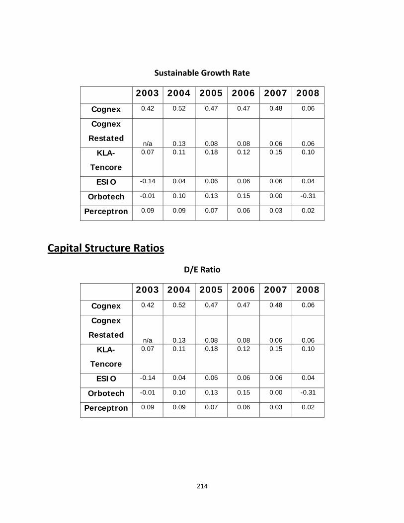
214
Sustainable Growth Rate
2003 2004 2005 2006 2007 2008
Cognex 0.42 0.52 0.47 0.47 0.48 0.06
Cognex
Restated n/a 0.13 0.08 0.08 0.06 0.06
KLA-
Tencore
0.07 0.11 0.18 0.12 0.15 0.10
ESIO -0.14 0.04 0.06 0.06 0.06 0.04
Orbotech -0.01 0.10 0.13 0.15 0.00 -0.31
Perceptron 0.09 0.09 0.07 0.06 0.03 0.02
Capital Structure Ratios
D/E Ratio
2003 2004 2005 2006 2007 2008
Cognex 0.42 0.52 0.47 0.47 0.48 0.06
Cognex
Restated n/a 0.13 0.08 0.08 0.06 0.06
KLA-
Tencore
0.07 0.11 0.18 0.12 0.15 0.10
ESIO -0.14 0.04 0.06 0.06 0.06 0.04
Orbotech -0.01 0.10 0.13 0.15 0.00 -0.31
Perceptron 0.09 0.09 0.07 0.06 0.03 0.02
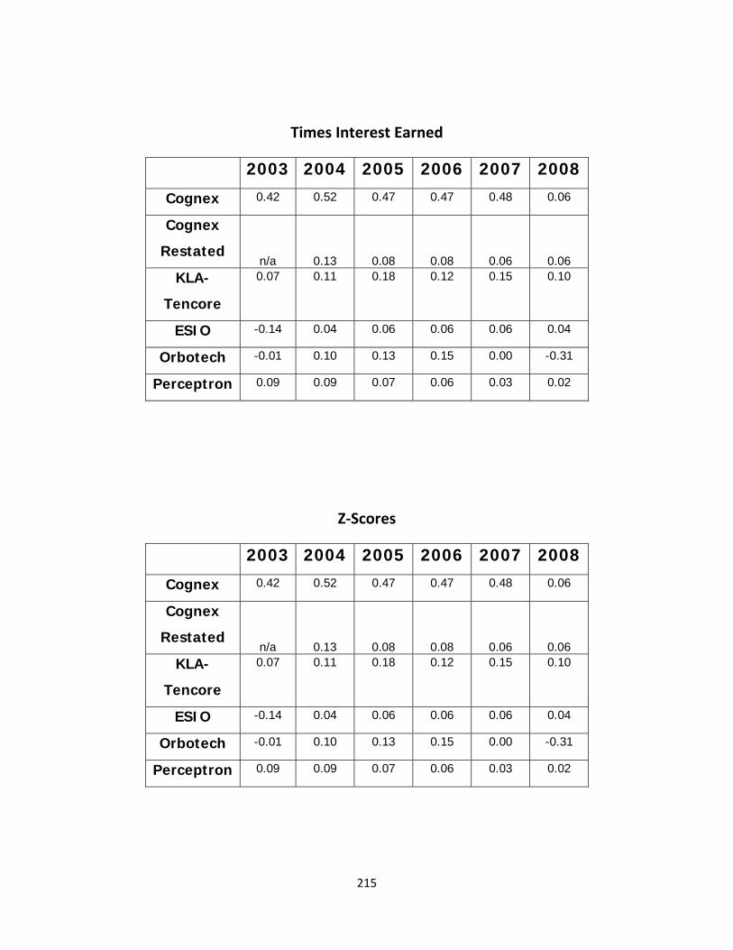
215
Times Interest Earned
2003 2004 2005 2006 2007 2008
Cognex 0.42 0.52 0.47 0.47 0.48 0.06
Cognex
Restated n/a 0.13 0.08 0.08 0.06 0.06
KLA-
Tencore
0.07 0.11 0.18 0.12 0.15 0.10
ESIO -0.14 0.04 0.06 0.06 0.06 0.04
Orbotech -0.01 0.10 0.13 0.15 0.00 -0.31
Perceptron 0.09 0.09 0.07 0.06 0.03 0.02
Z‐Scores
2003 2004 2005 2006 2007 2008
Cognex 0.42 0.52 0.47 0.47 0.48 0.06
Cognex
Restated n/a 0.13 0.08 0.08 0.06 0.06
KLA-
Tencore
0.07 0.11 0.18 0.12 0.15 0.10
ESIO -0.14 0.04 0.06 0.06 0.06 0.04
Orbotech -0.01 0.10 0.13 0.15 0.00 -0.31
Perceptron 0.09 0.09 0.07 0.06 0.03 0.02
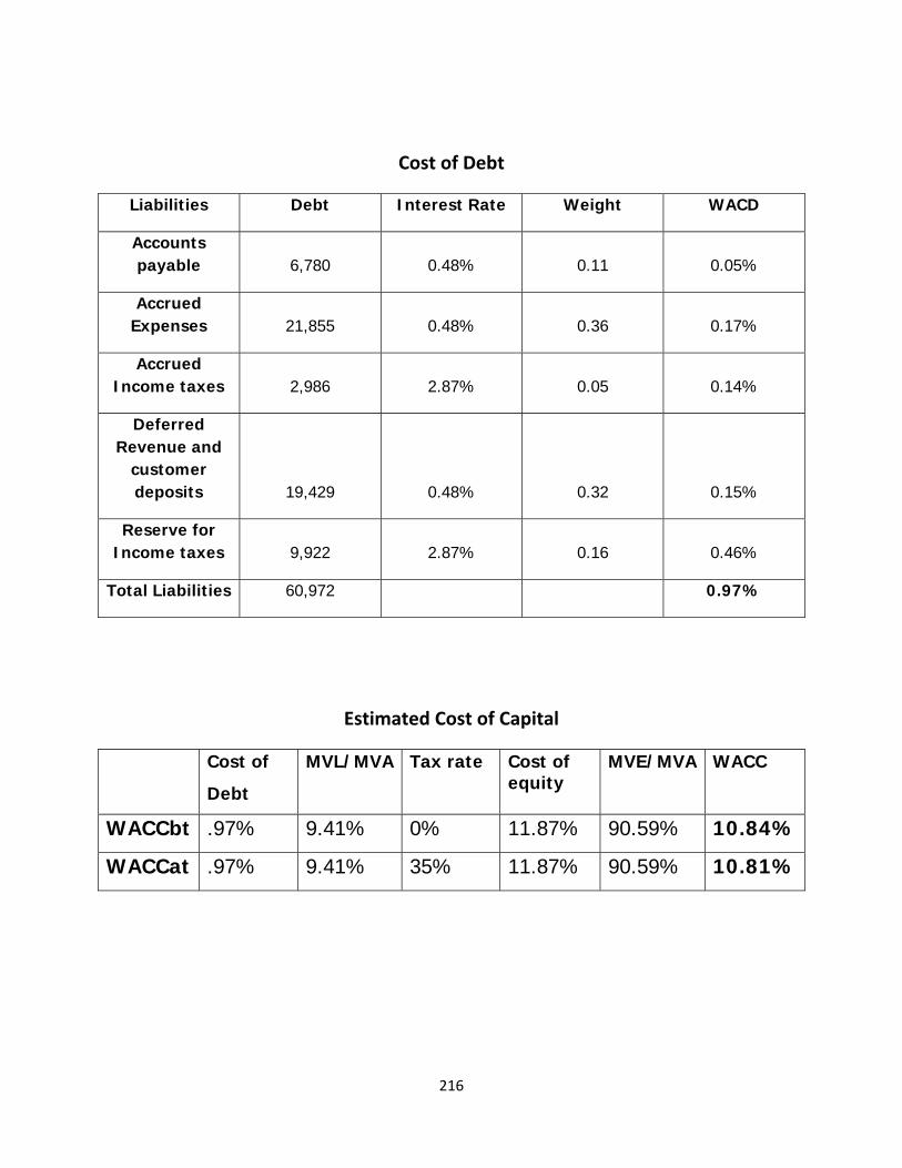
216
Cost of Debt
Liabilities Debt Interest Rate Weight WACD
Accounts payable 6,780 0.48% 0.11 0.05%
Accrued Expenses 21,855 0.48% 0.36 0.17%
Accrued Income taxes 2,986 2.87% 0.05 0.14%
Deferred Revenue and
customer deposits 19,429 0.48% 0.32 0.15%
Reserve for Income taxes 9,922 2.87% 0.16 0.46%
Total Liabilities 60,972 0.97%
Estimated Cost of Capital
Cost of
Debt
MVL/MVA Tax rate Cost of equity
MVE/MVA WACC
WACCbt .97% 9.41% 0% 11.87% 90.59% 10.84%
WACCat .97% 9.41% 35% 11.87% 90.59% 10.81%
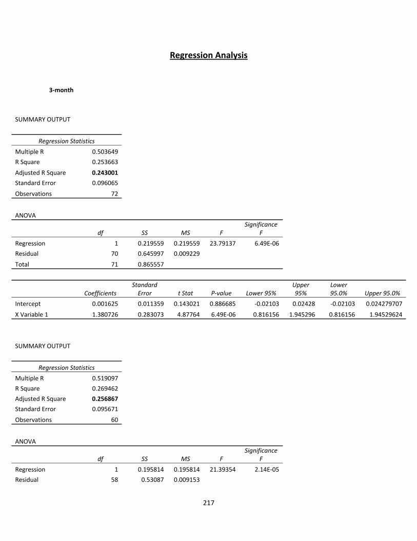
217
Regression Analysis
3‐month
SUMMARY OUTPUT
Regression Statistics
Multiple R 0.503649
R Square 0.253663
Adjusted R Square 0.243001
Standard Error 0.096065
Observations 72
ANOVA
df SS MS F Significance
F
Regression 1 0.219559 0.219559 23.79137 6.49E‐06
Residual 70 0.645997 0.009229
Total 71 0.865557
Coefficients Standard Error t Stat P‐value Lower 95%
Upper 95%
Lower 95.0% Upper 95.0%
Intercept 0.001625 0.011359 0.143021 0.886685 ‐0.02103 0.02428 ‐0.02103 0.024279707
X Variable 1 1.380726 0.283073 4.87764 6.49E‐06 0.816156 1.945296 0.816156 1.94529624
SUMMARY OUTPUT
Regression Statistics
Multiple R 0.519097
R Square 0.269462
Adjusted R Square 0.256867
Standard Error 0.095671
Observations 60
ANOVA
df SS MS F Significance
F
Regression 1 0.195814 0.195814 21.39354 2.14E‐05
Residual 58 0.53087 0.009153
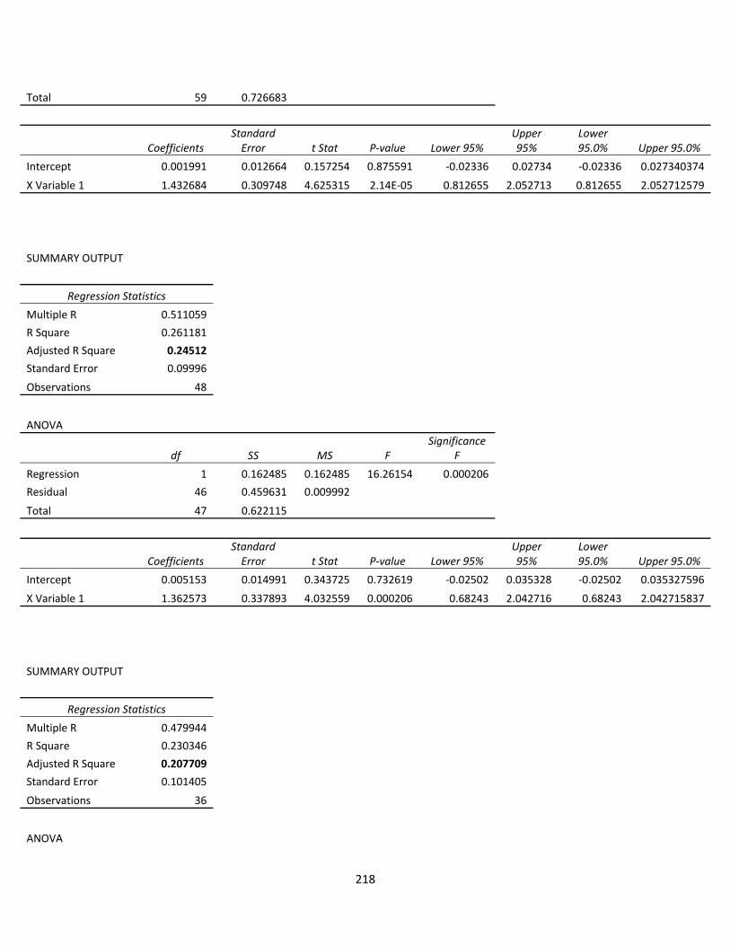
218
Total 59 0.726683
Coefficients Standard Error t Stat P‐value Lower 95%
Upper 95%
Lower 95.0% Upper 95.0%
Intercept 0.001991 0.012664 0.157254 0.875591 ‐0.02336 0.02734 ‐0.02336 0.027340374
X Variable 1 1.432684 0.309748 4.625315 2.14E‐05 0.812655 2.052713 0.812655 2.052712579
SUMMARY OUTPUT
Regression Statistics
Multiple R 0.511059
R Square 0.261181
Adjusted R Square 0.24512
Standard Error 0.09996
Observations 48
ANOVA
df SS MS F Significance
F
Regression 1 0.162485 0.162485 16.26154 0.000206
Residual 46 0.459631 0.009992
Total 47 0.622115
Coefficients Standard Error t Stat P‐value Lower 95%
Upper 95%
Lower 95.0% Upper 95.0%
Intercept 0.005153 0.014991 0.343725 0.732619 ‐0.02502 0.035328 ‐0.02502 0.035327596
X Variable 1 1.362573 0.337893 4.032559 0.000206 0.68243 2.042716 0.68243 2.042715837
SUMMARY OUTPUT
Regression Statistics
Multiple R 0.479944
R Square 0.230346
Adjusted R Square 0.207709
Standard Error 0.101405
Observations 36
ANOVA
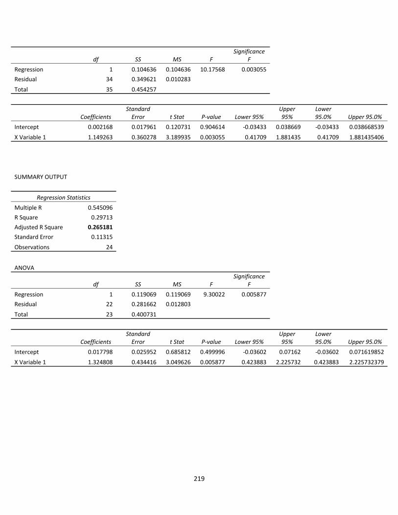
219
df SS MS F Significance
F
Regression 1 0.104636 0.104636 10.17568 0.003055
Residual 34 0.349621 0.010283
Total 35 0.454257
Coefficients Standard Error t Stat P‐value Lower 95%
Upper 95%
Lower 95.0% Upper 95.0%
Intercept 0.002168 0.017961 0.120731 0.904614 ‐0.03433 0.038669 ‐0.03433 0.038668539
X Variable 1 1.149263 0.360278 3.189935 0.003055 0.41709 1.881435 0.41709 1.881435406
SUMMARY OUTPUT
Regression Statistics
Multiple R 0.545096
R Square 0.29713
Adjusted R Square 0.265181
Standard Error 0.11315
Observations 24
ANOVA
df SS MS F Significance
F
Regression 1 0.119069 0.119069 9.30022 0.005877
Residual 22 0.281662 0.012803
Total 23 0.400731
Coefficients Standard Error t Stat P‐value Lower 95%
Upper 95%
Lower 95.0% Upper 95.0%
Intercept 0.017798 0.025952 0.685812 0.499996 ‐0.03602 0.07162 ‐0.03602 0.071619852
X Variable 1 1.324808 0.434416 3.049626 0.005877 0.423883 2.225732 0.423883 2.225732379
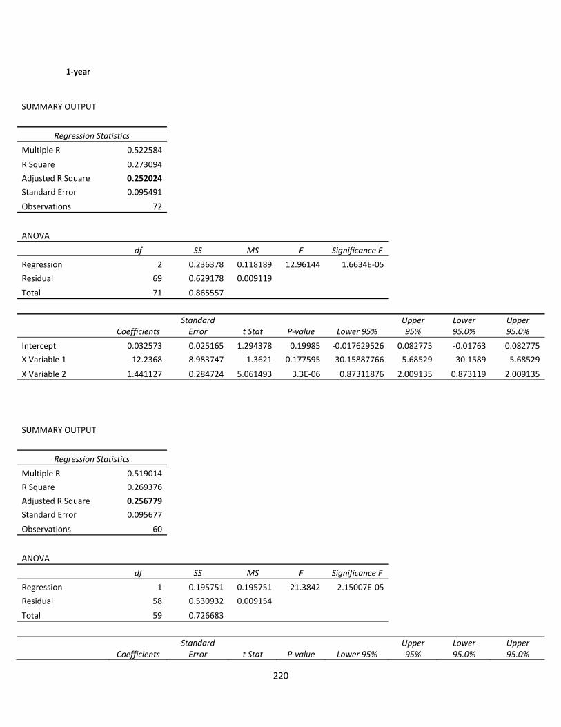
220
1‐year
SUMMARY OUTPUT
Regression Statistics
Multiple R 0.522584
R Square 0.273094
Adjusted R Square 0.252024
Standard Error 0.095491
Observations 72
ANOVA
df SS MS F Significance F
Regression 2 0.236378 0.118189 12.96144 1.6634E‐05
Residual 69 0.629178 0.009119
Total 71 0.865557
Coefficients Standard Error t Stat P‐value Lower 95%
Upper 95%
Lower 95.0%
Upper 95.0%
Intercept 0.032573 0.025165 1.294378 0.19985 ‐0.017629526 0.082775 ‐0.01763 0.082775
X Variable 1 ‐12.2368 8.983747 ‐1.3621 0.177595 ‐30.15887766 5.68529 ‐30.1589 5.68529
X Variable 2 1.441127 0.284724 5.061493 3.3E‐06 0.87311876 2.009135 0.873119 2.009135
SUMMARY OUTPUT
Regression Statistics
Multiple R 0.519014
R Square 0.269376
Adjusted R Square 0.256779
Standard Error 0.095677
Observations 60
ANOVA
df SS MS F Significance F
Regression 1 0.195751 0.195751 21.3842 2.15007E‐05
Residual 58 0.530932 0.009154
Total 59 0.726683
Coefficients Standard Error t Stat P‐value Lower 95%
Upper 95%
Lower 95.0%
Upper 95.0%
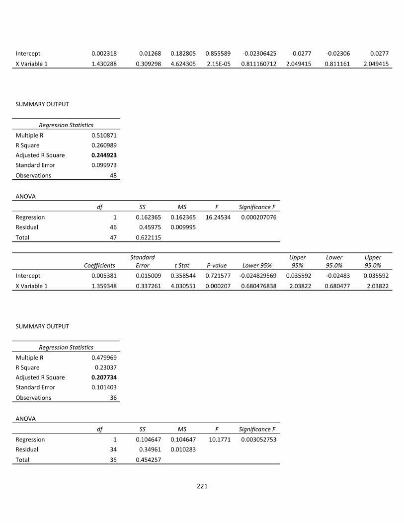
221
Intercept 0.002318 0.01268 0.182805 0.855589 ‐0.02306425 0.0277 ‐0.02306 0.0277
X Variable 1 1.430288 0.309298 4.624305 2.15E‐05 0.811160712 2.049415 0.811161 2.049415
SUMMARY OUTPUT
Regression Statistics
Multiple R 0.510871
R Square 0.260989
Adjusted R Square 0.244923
Standard Error 0.099973
Observations 48
ANOVA
df SS MS F Significance F
Regression 1 0.162365 0.162365 16.24534 0.000207076
Residual 46 0.45975 0.009995
Total 47 0.622115
Coefficients Standard Error t Stat P‐value Lower 95%
Upper 95%
Lower 95.0%
Upper 95.0%
Intercept 0.005381 0.015009 0.358544 0.721577 ‐0.024829569 0.035592 ‐0.02483 0.035592
X Variable 1 1.359348 0.337261 4.030551 0.000207 0.680476838 2.03822 0.680477 2.03822
SUMMARY OUTPUT
Regression Statistics
Multiple R 0.479969
R Square 0.23037
Adjusted R Square 0.207734
Standard Error 0.101403
Observations 36
ANOVA
df SS MS F Significance F
Regression 1 0.104647 0.104647 10.1771 0.003052753
Residual 34 0.34961 0.010283
Total 35 0.454257
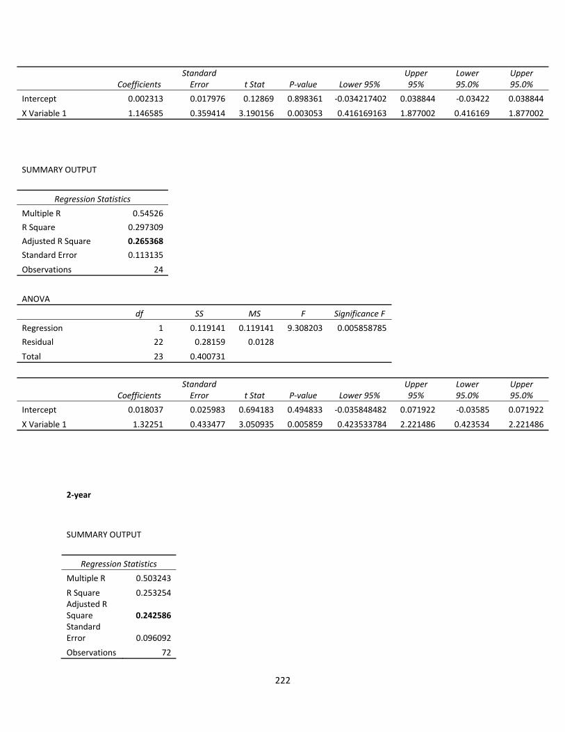
222
2‐year
Coefficients Standard Error t Stat P‐value Lower 95%
Upper 95%
Lower 95.0%
Upper 95.0%
Intercept 0.002313 0.017976 0.12869 0.898361 ‐0.034217402 0.038844 ‐0.03422 0.038844
X Variable 1 1.146585 0.359414 3.190156 0.003053 0.416169163 1.877002 0.416169 1.877002
SUMMARY OUTPUT
Regression Statistics
Multiple R 0.54526
R Square 0.297309
Adjusted R Square 0.265368
Standard Error 0.113135
Observations 24
ANOVA
df SS MS F Significance F
Regression 1 0.119141 0.119141 9.308203 0.005858785
Residual 22 0.28159 0.0128
Total 23 0.400731
Coefficients Standard Error t Stat P‐value Lower 95%
Upper 95%
Lower 95.0%
Upper 95.0%
Intercept 0.018037 0.025983 0.694183 0.494833 ‐0.035848482 0.071922 ‐0.03585 0.071922
X Variable 1 1.32251 0.433477 3.050935 0.005859 0.423533784 2.221486 0.423534 2.221486
SUMMARY OUTPUT
Regression Statistics
Multiple R 0.503243
R Square 0.253254 Adjusted R Square 0.242586 Standard Error 0.096092
Observations 72
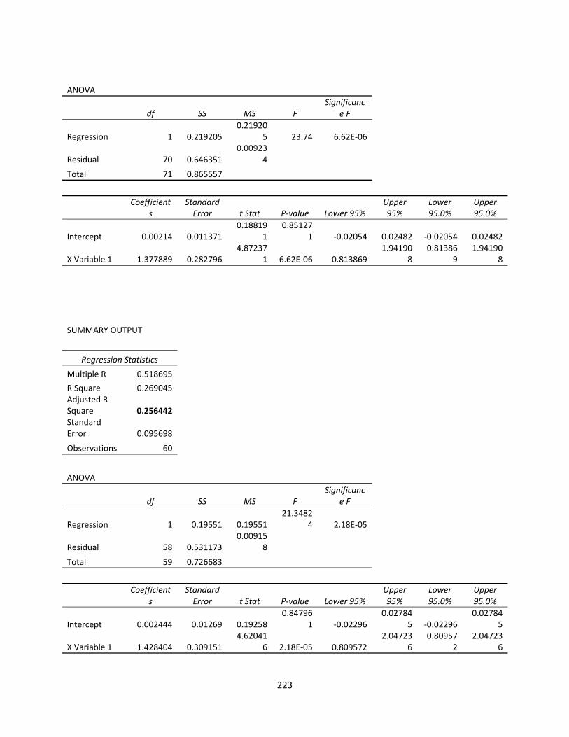
223
ANOVA
df SS MS F Significanc
e F
Regression 1 0.219205 0.21920
5 23.74 6.62E‐06
Residual 70 0.646351 0.00923
4
Total 71 0.865557
Coefficient
s Standard Error t Stat P‐value Lower 95%
Upper 95%
Lower 95.0%
Upper 95.0%
Intercept 0.00214 0.011371 0.18819
1 0.85127
1 ‐0.02054 0.02482 ‐0.02054 0.02482
X Variable 1 1.377889 0.282796 4.87237
1 6.62E‐06 0.813869 1.94190
8 0.81386
9 1.94190
8
SUMMARY OUTPUT
Regression Statistics
Multiple R 0.518695
R Square 0.269045 Adjusted R Square 0.256442 Standard Error 0.095698
Observations 60
ANOVA
df SS MS F Significanc
e F
Regression 1 0.19551 0.19551 21.3482
4 2.18E‐05
Residual 58 0.531173 0.00915
8
Total 59 0.726683
Coefficient
s Standard Error t Stat P‐value Lower 95%
Upper 95%
Lower 95.0%
Upper 95.0%
Intercept 0.002444 0.01269 0.19258 0.84796
1 ‐0.02296 0.02784
5 ‐0.02296 0.02784
5
X Variable 1 1.428404 0.309151 4.62041
6 2.18E‐05 0.809572 2.04723
6 0.80957
2 2.04723
6
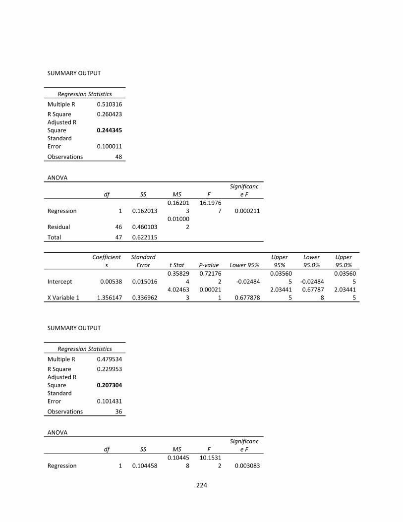
224
SUMMARY OUTPUT
Regression Statistics
Multiple R 0.510316
R Square 0.260423 Adjusted R Square 0.244345 Standard Error 0.100011
Observations 48
ANOVA
df SS MS F Significanc
e F
Regression 1 0.162013 0.16201
3 16.1976
7 0.000211
Residual 46 0.460103 0.01000
2
Total 47 0.622115
Coefficient
s Standard Error t Stat P‐value Lower 95%
Upper 95%
Lower 95.0%
Upper 95.0%
Intercept 0.00538 0.015016 0.35829
4 0.72176
2 ‐0.02484 0.03560
5 ‐0.02484 0.03560
5
X Variable 1 1.356147 0.336962 4.02463
3 0.00021
1 0.677878 2.03441
5 0.67787
8 2.03441
5
SUMMARY OUTPUT
Regression Statistics
Multiple R 0.479534
R Square 0.229953 Adjusted R Square 0.207304 Standard Error 0.101431
Observations 36
ANOVA
df SS MS F Significanc
e F
Regression 1 0.104458 0.10445
8 10.1531
2 0.003083
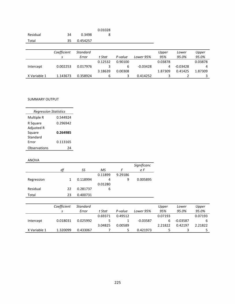
225
Residual 34 0.3498 0.01028
8
Total 35 0.454257
Coefficient
s Standard Error t Stat P‐value Lower 95%
Upper 95%
Lower 95.0%
Upper 95.0%
Intercept 0.002253 0.017976 0.12532
3 0.90100
6 ‐0.03428 0.03878
4 ‐0.03428 0.03878
4
X Variable 1 1.143673 0.358924 3.18639
6 0.00308
3 0.414252 1.87309
3 0.41425
2 1.87309
3
SUMMARY OUTPUT
Regression Statistics
Multiple R 0.544924
R Square 0.296942 Adjusted R Square 0.264985 Standard Error 0.113165
Observations 24
ANOVA
df SS MS F Significanc
e F
Regression 1 0.118994 0.11899
4 9.29186
9 0.005895
Residual 22 0.281737 0.01280
6
Total 23 0.400731
Coefficient
s Standard Error t Stat P‐value Lower 95%
Upper 95%
Lower 95.0%
Upper 95.0%
Intercept 0.018031 0.025992 0.69371
5 0.49512
1 ‐0.03587 0.07193
6 ‐0.03587 0.07193
6
X Variable 1 1.320099 0.433067 3.04825
7 0.00589
5 0.421973 2.21822
5 0.42197
3 2.21822
5
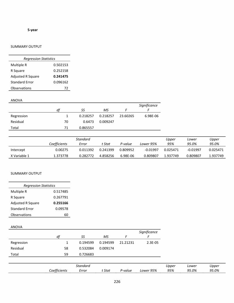
226
5‐year
SUMMARY OUTPUT
Regression Statistics
Multiple R 0.502153
R Square 0.252158
Adjusted R Square 0.241475
Standard Error 0.096162
Observations 72
ANOVA
df SS MS F Significance
F
Regression 1 0.218257 0.218257 23.60265 6.98E‐06
Residual 70 0.6473 0.009247
Total 71 0.865557
Coefficients Standard Error t Stat P‐value Lower 95%
Upper 95%
Lower 95.0%
Upper 95.0%
Intercept 0.00275 0.011392 0.241399 0.809952 ‐0.01997 0.025471 ‐0.01997 0.025471
X Variable 1 1.373778 0.282772 4.858256 6.98E‐06 0.809807 1.937749 0.809807 1.937749
SUMMARY OUTPUT
Regression Statistics
Multiple R 0.517485
R Square 0.267791
Adjusted R Square 0.255166
Standard Error 0.09578
Observations 60
ANOVA
df SS MS F Significance
F
Regression 1 0.194599 0.194599 21.21231 2.3E‐05
Residual 58 0.532084 0.009174
Total 59 0.726683
Coefficients Standard Error t Stat P‐value Lower 95%
Upper 95%
Lower 95.0%
Upper 95.0%
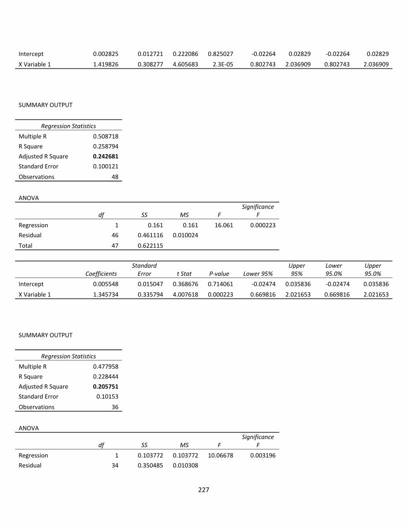
227
Intercept 0.002825 0.012721 0.222086 0.825027 ‐0.02264 0.02829 ‐0.02264 0.02829
X Variable 1 1.419826 0.308277 4.605683 2.3E‐05 0.802743 2.036909 0.802743 2.036909
SUMMARY OUTPUT
Regression Statistics
Multiple R 0.508718
R Square 0.258794
Adjusted R Square 0.242681
Standard Error 0.100121
Observations 48
ANOVA
df SS MS F Significance
F
Regression 1 0.161 0.161 16.061 0.000223
Residual 46 0.461116 0.010024
Total 47 0.622115
Coefficients Standard Error t Stat P‐value Lower 95%
Upper 95%
Lower 95.0%
Upper 95.0%
Intercept 0.005548 0.015047 0.368676 0.714061 ‐0.02474 0.035836 ‐0.02474 0.035836
X Variable 1 1.345734 0.335794 4.007618 0.000223 0.669816 2.021653 0.669816 2.021653
SUMMARY OUTPUT
Regression Statistics
Multiple R 0.477958
R Square 0.228444
Adjusted R Square 0.205751
Standard Error 0.10153
Observations 36
ANOVA
df SS MS F Significance
F
Regression 1 0.103772 0.103772 10.06678 0.003196
Residual 34 0.350485 0.010308
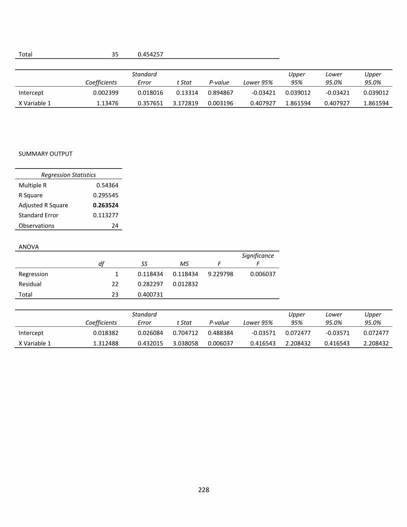
228
Total 35 0.454257
Coefficients Standard Error t Stat P‐value Lower 95%
Upper 95%
Lower 95.0%
Upper 95.0%
Intercept 0.002399 0.018016 0.13314 0.894867 ‐0.03421 0.039012 ‐0.03421 0.039012
X Variable 1 1.13476 0.357651 3.172819 0.003196 0.407927 1.861594 0.407927 1.861594
SUMMARY OUTPUT
Regression Statistics
Multiple R 0.54364
R Square 0.295545
Adjusted R Square 0.263524
Standard Error 0.113277
Observations 24
ANOVA
df SS MS F Significance
F
Regression 1 0.118434 0.118434 9.229798 0.006037
Residual 22 0.282297 0.012832
Total 23 0.400731
Coefficients Standard Error t Stat P‐value Lower 95%
Upper 95%
Lower 95.0%
Upper 95.0%
Intercept 0.018382 0.026084 0.704712 0.488384 ‐0.03571 0.072477 ‐0.03571 0.072477
X Variable 1 1.312488 0.432015 3.038058 0.006037 0.416543 2.208432 0.416543 2.208432
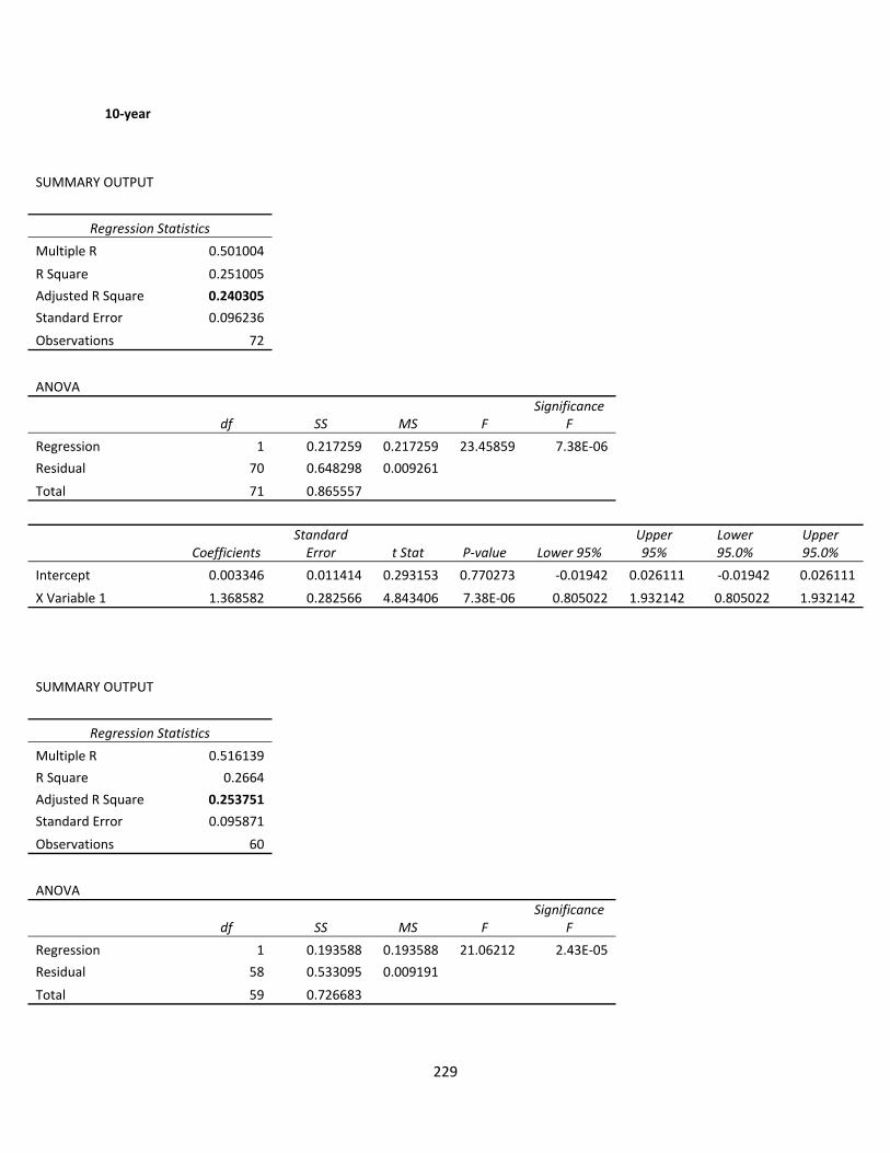
229
10‐year
SUMMARY OUTPUT
Regression Statistics
Multiple R 0.501004
R Square 0.251005
Adjusted R Square 0.240305
Standard Error 0.096236
Observations 72
ANOVA
df SS MS F Significance
F
Regression 1 0.217259 0.217259 23.45859 7.38E‐06
Residual 70 0.648298 0.009261
Total 71 0.865557
Coefficients Standard Error t Stat P‐value Lower 95%
Upper 95%
Lower 95.0%
Upper 95.0%
Intercept 0.003346 0.011414 0.293153 0.770273 ‐0.01942 0.026111 ‐0.01942 0.026111
X Variable 1 1.368582 0.282566 4.843406 7.38E‐06 0.805022 1.932142 0.805022 1.932142
SUMMARY OUTPUT
Regression Statistics
Multiple R 0.516139
R Square 0.2664
Adjusted R Square 0.253751
Standard Error 0.095871
Observations 60
ANOVA
df SS MS F Significance
F
Regression 1 0.193588 0.193588 21.06212 2.43E‐05
Residual 58 0.533095 0.009191
Total 59 0.726683
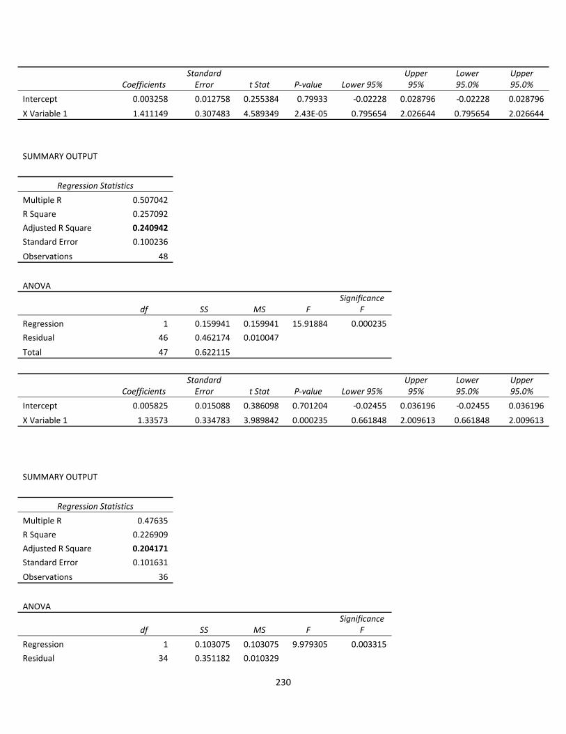
230
Coefficients Standard Error t Stat P‐value Lower 95%
Upper 95%
Lower 95.0%
Upper 95.0%
Intercept 0.003258 0.012758 0.255384 0.79933 ‐0.02228 0.028796 ‐0.02228 0.028796
X Variable 1 1.411149 0.307483 4.589349 2.43E‐05 0.795654 2.026644 0.795654 2.026644
SUMMARY OUTPUT
Regression Statistics
Multiple R 0.507042
R Square 0.257092
Adjusted R Square 0.240942
Standard Error 0.100236
Observations 48
ANOVA
df SS MS F Significance
F
Regression 1 0.159941 0.159941 15.91884 0.000235
Residual 46 0.462174 0.010047
Total 47 0.622115
Coefficients Standard Error t Stat P‐value Lower 95%
Upper 95%
Lower 95.0%
Upper 95.0%
Intercept 0.005825 0.015088 0.386098 0.701204 ‐0.02455 0.036196 ‐0.02455 0.036196
X Variable 1 1.33573 0.334783 3.989842 0.000235 0.661848 2.009613 0.661848 2.009613
SUMMARY OUTPUT
Regression Statistics
Multiple R 0.47635
R Square 0.226909
Adjusted R Square 0.204171
Standard Error 0.101631
Observations 36
ANOVA
df SS MS F Significance
F
Regression 1 0.103075 0.103075 9.979305 0.003315
Residual 34 0.351182 0.010329
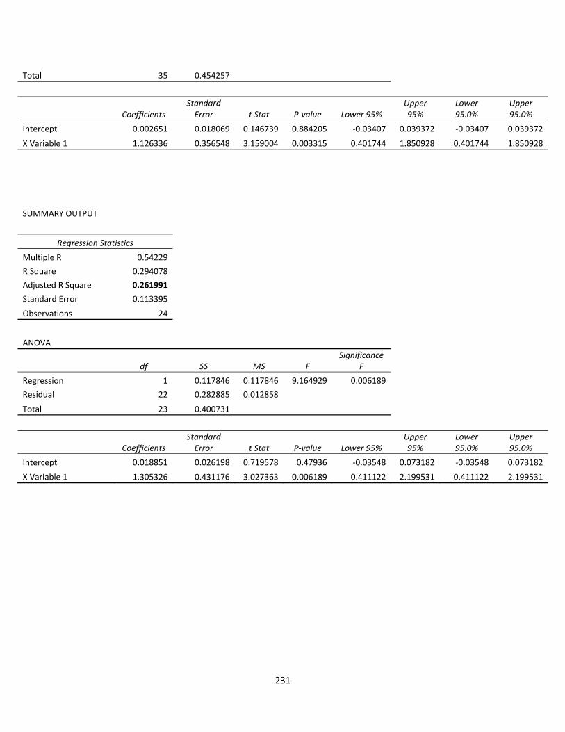
231
Total 35 0.454257
Coefficients Standard Error t Stat P‐value Lower 95%
Upper 95%
Lower 95.0%
Upper 95.0%
Intercept 0.002651 0.018069 0.146739 0.884205 ‐0.03407 0.039372 ‐0.03407 0.039372
X Variable 1 1.126336 0.356548 3.159004 0.003315 0.401744 1.850928 0.401744 1.850928
SUMMARY OUTPUT
Regression Statistics
Multiple R 0.54229
R Square 0.294078
Adjusted R Square 0.261991
Standard Error 0.113395
Observations 24
ANOVA
df SS MS F Significance
F
Regression 1 0.117846 0.117846 9.164929 0.006189
Residual 22 0.282885 0.012858
Total 23 0.400731
Coefficients Standard Error t Stat P‐value Lower 95%
Upper 95%
Lower 95.0%
Upper 95.0%
Intercept 0.018851 0.026198 0.719578 0.47936 ‐0.03548 0.073182 ‐0.03548 0.073182
X Variable 1 1.305326 0.431176 3.027363 0.006189 0.411122 2.199531 0.411122 2.199531
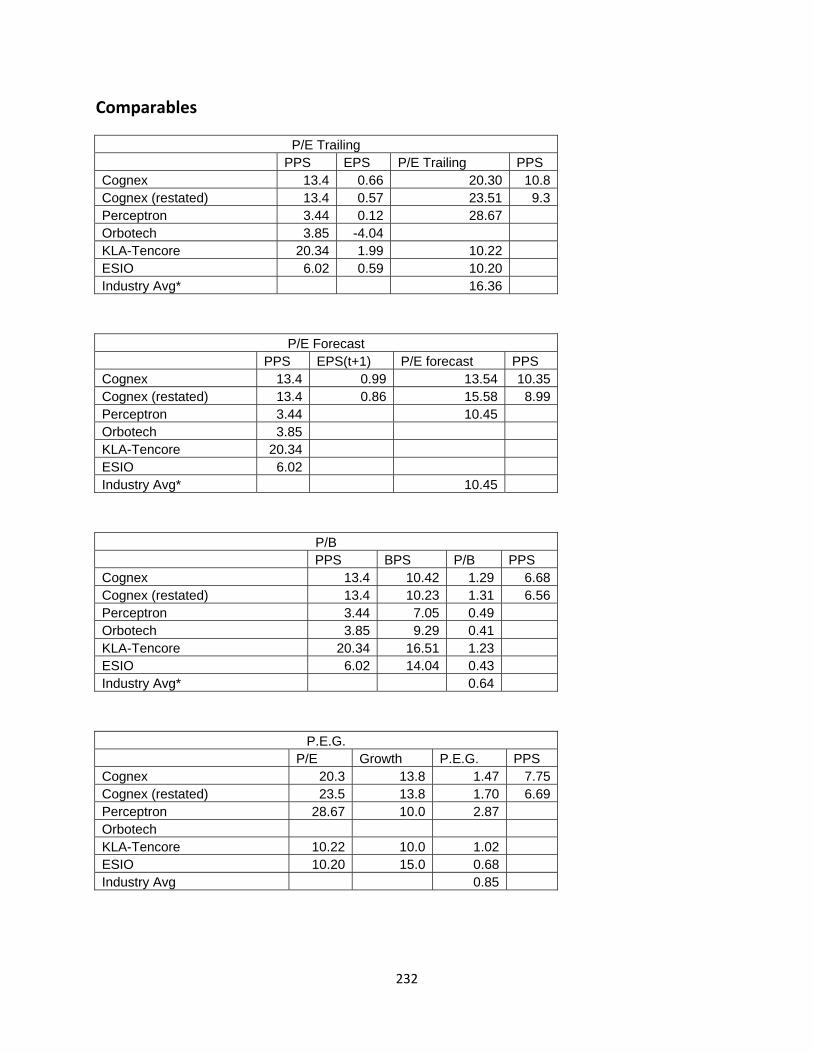
232
Comparables
P/E Trailing PPS EPS P/E Trailing PPS Cognex 13.4 0.66 20.30 10.8Cognex (restated) 13.4 0.57 23.51 9.3Perceptron 3.44 0.12 28.67 Orbotech 3.85 -4.04 KLA-Tencore 20.34 1.99 10.22 ESIO 6.02 0.59 10.20 Industry Avg* 16.36
P/E Forecast PPS EPS(t+1) P/E forecast PPS Cognex 13.4 0.99 13.54 10.35Cognex (restated) 13.4 0.86 15.58 8.99Perceptron 3.44 10.45 Orbotech 3.85 KLA-Tencore 20.34 ESIO 6.02 Industry Avg* 10.45
P/B PPS BPS P/B PPS Cognex 13.4 10.42 1.29 6.68Cognex (restated) 13.4 10.23 1.31 6.56Perceptron 3.44 7.05 0.49 Orbotech 3.85 9.29 0.41 KLA-Tencore 20.34 16.51 1.23 ESIO 6.02 14.04 0.43 Industry Avg* 0.64
P.E.G. P/E Growth P.E.G. PPS Cognex 20.3 13.8 1.47 7.75Cognex (restated) 23.5 13.8 1.70 6.69Perceptron 28.67 10.0 2.87 Orbotech KLA-Tencore 10.22 10.0 1.02 ESIO 10.20 15.0 0.68 Industry Avg 0.85
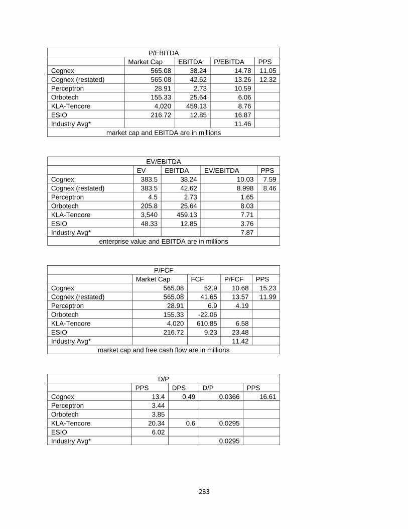
233
P/EBITDA Market Cap EBITDA P/EBITDA PPS Cognex 565.08 38.24 14.78 11.05Cognex (restated) 565.08 42.62 13.26 12.32Perceptron 28.91 2.73 10.59 Orbotech 155.33 25.64 6.06 KLA-Tencore 4,020 459.13 8.76 ESIO 216.72 12.85 16.87 Industry Avg* 11.46
market cap and EBITDA are in millions
EV/EBITDA EV EBITDA EV/EBITDA PPS Cognex 383.5 38.24 10.03 7.59Cognex (restated) 383.5 42.62 8.998 8.46Perceptron 4.5 2.73 1.65 Orbotech 205.8 25.64 8.03 KLA-Tencore 3,540 459.13 7.71 ESIO 48.33 12.85 3.76 Industry Avg* 7.87
enterprise value and EBITDA are in millions
P/FCF Market Cap FCF P/FCF PPS Cognex 565.08 52.9 10.68 15.23Cognex (restated) 565.08 41.65 13.57 11.99Perceptron 28.91 6.9 4.19 Orbotech 155.33 -22.06 KLA-Tencore 4,020 610.85 6.58 ESIO 216.72 9.23 23.48 Industry Avg* 11.42
market cap and free cash flow are in millions
D/P PPS DPS D/P PPS Cognex 13.4 0.49 0.0366 16.61Perceptron 3.44 Orbotech 3.85 KLA-Tencore 20.34 0.6 0.0295 ESIO 6.02 Industry Avg* 0.0295
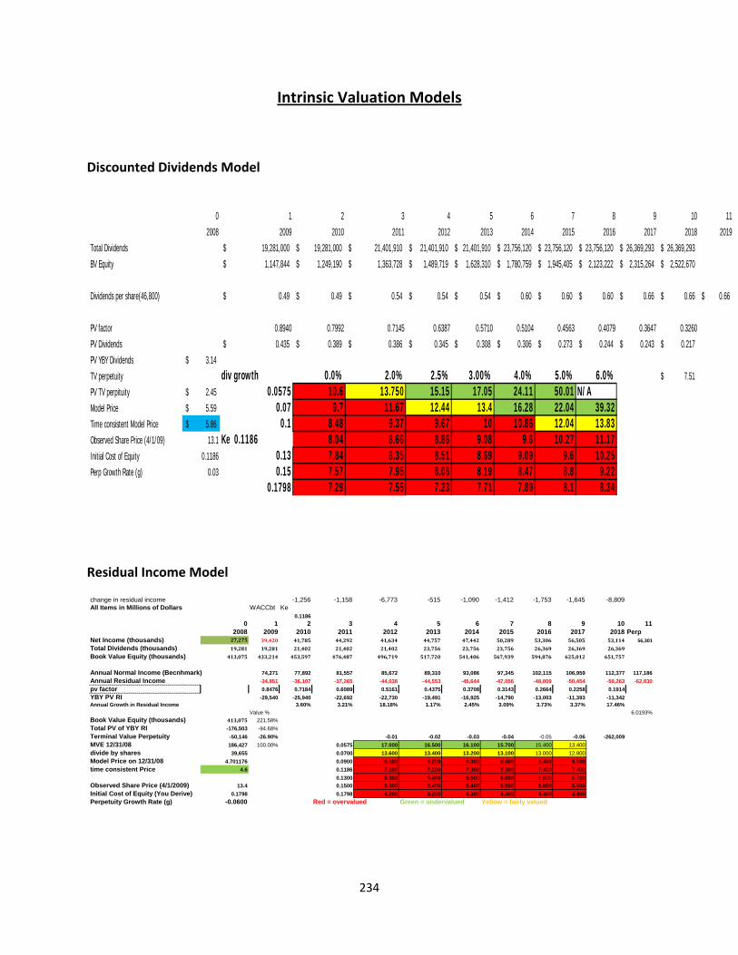
234
Intrinsic Valuation Models
Discounted Dividends Model
Residual Income Model
0 1 2 3 4 5 6 7 8 9 10 112008 2009 2010 2011 2012 2013 2014 2015 2016 2017 2018 2019
Total Dividends 19,281,000$ 19,281,000$ 21,401,910$ 21,401,910$ 21,401,910$ 23,756,120$ 23,756,120$ 23,756,120$ 26,369,293$ 26,369,293$ BV Equity 1,147,844$ 1,249,190$ 1,363,728$ 1,489,719$ 1,628,310$ 1,780,759$ 1,945,405$ 2,123,222$ 2,315,264$ 2,522,670$
Dividends per share(46,800) 0.49$ 0.49$ 0.54$ 0.54$ 0.54$ 0.60$ 0.60$ 0.60$ 0.66$ 0.66$ 0.66$
PV factor 0.8940 0.7992 0.7145 0.6387 0.5710 0.5104 0.4563 0.4079 0.3647 0.3260PV Dividends 0.435$ 0.389$ 0.386$ 0.345$ 0.308$ 0.306$ 0.273$ 0.244$ 0.243$ 0.217$ PV YBY Dividends 3.14$ TV perpetuity div growth 0.0% 2.0% 2.5% 3.00% 4.0% 5.0% 6.0% 7.51$ PV TV perpituity 2.45$ 0.0575 10.6 13.750 15.15 17.05 24.11 50.01 N/AModel Price 5.59$ 0.07 9.7 11.67 12.44 13.4 16.28 22.04 39.32Time consistent Model Price 5.86$ 0.1 8.48 9.37 9.67 10 10.86 12.04 13.83Observed Share Price (4/1/09) 13.1 Ke 0.1186 8.04 8.66 8.86 9.08 9.6 10.27 11.17Initial Cost of Equity 0.1186 0.13 7.84 8.35 8.51 8.69 9.09 9.6 10.25Perp Growth Rate (g) 0.03 0.15 7.57 7.95 8.06 8.19 8.47 8.8 9.22
0.1798 7.29 7.55 7.23 7.71 7.89 8.1 8.34
change in residual income -1,256 -1,158 -6,773 -515 -1,090 -1,412 -1,753 -1,645 -8,809All Items in Millions of Dollars WACCbt Ke
0.11860 1 2 3 4 5 6 7 8 9 10 11
2008 2009 2010 2011 2012 2013 2014 2015 2016 2017 2018 PerpNet Income (thousands) 27,275 39,420 41,785 44,292 41,634 44,757 47,442 50,289 53,306 56,505 53,114 56,301
Total Dividends (thousands) 19,281 19,281 21,402 21,402 21,402 23,756 23,756 23,756 26,369 26,369 26,369
Book Value Equity (thousands) 413,075 433,214 453,597 476,487 496,719 517,720 541,406 567,939 594,876 625,012 651,757
Annual Normal Income (Becnhmark) 74,271 77,892 81,557 85,672 89,310 93,086 97,345 102,115 106,959 112,377 117,186Annual Residual Income -34,851 -36,107 -37,265 -44,038 -44,553 -45,644 -47,056 -48,809 -50,454 -59,263 -62,830pv factor 0.8476 0.7184 0.6089 0.5161 0.4375 0.3708 0.3143 0.2664 0.2258 0.1914YBY PV RI -29,540 -25,940 -22,692 -22,730 -19,491 -16,925 -14,790 -13,003 -11,393 -11,342Annual Growth in Residual Income 3.60% 3.21% 18.18% 1.17% 2.45% 3.09% 3.73% 3.37% 17.46%
Value % 6.0193%Book Value Equity (thousands) 413,075 221.58%Total PV of YBY RI -176,503 -94.68%Terminal Value Perpetuity -50,146 -26.90% -0.01 -0.02 -0.03 -0.04 -0.05 -0.06 -262,009MVE 12/31/08 186,427 100.00% 0.0575 17.000 16.500 16.100 15.700 15.400 13.400divide by shares 39,655 0.0700 13.600 13.400 13.200 13.100 13.000 12.800Model Price on 12/31/08 4.701176 0.0900 9.100 9.200 9.300 9.400 9.400 9.500time consistent Price 4.6 0.1186 7.100 7.200 7.300 7.300 7.400 7.400
0.1300 6.300 6.400 6.500 6.600 6.600 6.700Observed Share Price (4/1/2009) 13.4 0.1500 5.300 5.400 5.400 5.500 5.600 5.600Initial Cost of Equity (You Derive) 0.1798 0.1798 4.200 4.200 4.300 4.400 4.400 4.400Perpetuity Growth Rate (g) -0.0600 Red = overvalued Green = undervalued Yellow = fairly valued
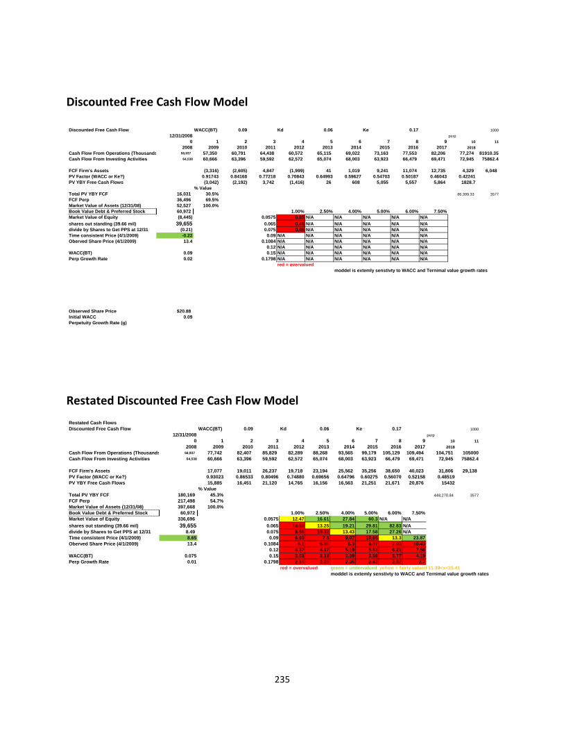
235
Discounted Free Cash Flow Model
Restated Discounted Free Cash Flow Model
Discounted Free Cash Flow WACC(BT) 0.09 Kd 0.06 Ke 0.17 100012/31/2008 perp
0 1 2 3 4 5 6 7 8 9 10 112008 2009 2010 2011 2012 2013 2014 2015 2016 2017 2018
Cash Flow From Operations (Thousands 58,937 57,350 60,791 64,438 60,572 65,115 69,022 73,163 77,553 82,206 77,274 81910.35Cash Flow From Investing Activities 64,538 60,666 63,396 59,592 62,572 65,074 68,003 63,923 66,479 69,471 72,945 75862.4
FCF Firm's Assets (3,316) (2,605) 4,847 (1,999) 41 1,019 9,241 11,074 12,735 4,329 6,048 PV Factor (WACC or Ke?) 0.91743 0.84168 0.77218 0.70843 0.64993 0.59627 0.54703 0.50187 0.46043 0.42241PV YBY Free Cash Flows (3,042) (2,192) 3,742 (1,416) 26 608 5,055 5,557 5,864 1828.7
% ValueTotal PV YBY FCF 16,031 30.5% 86,399.33 3577FCF Perp 36,496 69.5%Market Value of Assets (12/31/08) 52,527 100.0%Book Value Debt & Preferred Stock 60,972 1.00% 2.50% 4.00% 5.00% 6.00% 7.50%Market Value of Equity (8,445) 0.0575 0.85 N/A N/A N/A N/A N/Ashares out standing (39.66 mil) 39,655 0.065 0.45 N/A N/A N/A N/A N/Adivide by Shares to Get PPS at 12/31 (0.21) 0.075 0.06 N/A N/A N/A N/A N/ATime consistent Price (4/1/2009) -0.22 0.09 N/A N/A N/A N/A N/A N/AOberved Share Price (4/1/2009) 13.4 0.1084 N/A N/A N/A N/A N/A N/A
0.12 N/A N/A N/A N/A N/A N/AWACC(BT) 0.09 0.15 N/A N/A N/A N/A N/A N/APerp Growth Rate 0.02 0.1798 N/A N/A N/A N/A N/A N/A
red = overvaluedmoddel is extemly senstivty to WACC and Ternimal value growth rates
Observed Share Price $20.88Initial WACC 0.09Perpetuity Growth Rate (g)
Restated Cash FlowsDiscounted Free Cash Flow WACC(BT) 0.09 Kd 0.06 Ke 0.17 1000
12/31/2008 perp0 1 2 3 4 5 6 7 8 9 10 11
2008 2009 2010 2011 2012 2013 2014 2015 2016 2017 2018Cash Flow From Operations (Thousands 58,937 77,742 82,407 85,829 82,289 88,268 93,565 99,179 105,129 109,494 104,751 105000Cash Flow From Investing Activities 64,538 60,666 63,396 59,592 62,572 65,074 68,003 63,923 66,479 69,471 72,945 75862.4
FCF Firm's Assets 17,077 19,011 26,237 19,718 23,194 25,562 35,256 38,650 40,023 31,806 29,138 PV Factor (WACC or Ke?) 0.93023 0.86533 0.80496 0.74880 0.69656 0.64796 0.60275 0.56070 0.52158 0.48519PV YBY Free Cash Flows 15,885 16,451 21,120 14,765 16,156 16,563 21,251 21,671 20,876 15432
% ValueTotal PV YBY FCF 180,169 45.3% 448,270.84 3577FCF Perp 217,498 54.7%Market Value of Assets (12/31/08) 397,668 100.0%Book Value Debt & Preferred Stock 60,972 1.00% 2.50% 4.00% 5.00% 6.00% 7.50%Market Value of Equity 336,696 0.0575 12.47 16.61 27.84 60.3 N/A N/Ashares out standing (39.66 mil) 39,655 0.065 10.53 13.25 19.21 29.81 82.83 N/Adivide by Shares to Get PPS at 12/31 8.49 0.075 8.65 10.32 13.43 17.58 27.26 N/ATime consistent Price (4/1/2009) 8.65 0.09 6.69 7.6 9.07 10.65 13.3 23.87Oberved Share Price (4/1/2009) 13.4 0.1084 5.1 5.59 6.3 6.97 7.93 10.43
0.12 4.37 4.17 5.19 5.63 6.21 7.56WACC(BT) 0.075 0.15 3.03 3.19 3.39 3.56 3.77 4.19Perp Growth Rate 0.01 0.1798 2.16 2.25 2.35 2.43 2.52 2.7
red = overvalued green = undervalued yellow = fairly valued 11.39<x<15.41moddel is extemly senstivty to WACC and Ternimal value growth rates
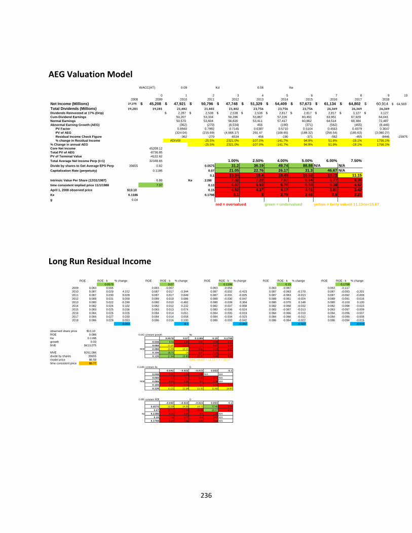
236
AEG Valuation Model
Long Run Residual Income
WACC(AT) 0.09 Kd 0.06 Ke
0 1 2 3 4 5 6 7 8 9 102008 2009 2010 2011 2012 2013 2014 2015 2016 2017 2018
Net Income (Millions) 27,275 45,208$ 47,921$ 50,796$ 47,748$ 51,329$ 54,409$ 57,673$ 61,134$ 64,802$ 60,914$ 64,569$ Total Dividends (Millions) 19,281 19,281 21,402 21,402 21,402 23,756 23,756 23,756 26,369 26,369 26,369Dividends Reinvested at 17% (Drip) 2,287$ 2,538$ 2,538$ 2,538$ 2,817$ 2,817$ 2,817$ 3,127$ 3,127$ Cum-Dividend Earnings 50,207 53,334 50,286 53,867 57,226 60,491 63,951 67,929 64,041 Normal Earnings 50,570 53,604 56,820 53,411 57,417 60,862 64,514 68,384 72,487 Abnormal Earning Growth (AEG) (362) (270) (6,534) 456 (190) (371) (562) (455) (8,446)
PV Factor 0.8940 0.7992 0.7145 0.6387 0.5710 0.5104 0.4563 0.4079 0.3647PV of AEG (324.04) (215.69) (4,668.17) 291.47 (108.65) (189.32) (256.54) (185.63) (3,080.27) Residual Income Check Figure -362 -270 -6534 456 -190 -371 -562 -455 -8446 -23975% change in Residual Income #DIV/0! -25.5% 2321.0% -107.0% -141.7% 94.9% 51.6% -19.1% 1756.1%
% Change in annual AEG -25.5% 2321.0% -107.0% -141.7% 94.9% 51.6% -19.1% 1756.1%Core Net Income 45208.12Total PV of AEG -8736.85PV of Terminal Value -4122.62Total Average Net Income Perp (t+1) 32348.65 1.00% 2.50% 4.00% 5.00% 6.00% 7.50%Divide by shares to Get Average EPS Perp 39655 0.82 0.0575 31.2 36.19 49.74 88.88 N/A N/ACapitalization Rate (perpetuity) 0.1186 0.07 21.05 22.76 26.17 31.3 46.67 N/A
0.1 10.34 10.4 10.49 10.58 10.73 11.15Intrinsic Value Per Share (12/31/1987) 6.88 Ke .1186 7.32 7.22 7.07 6.94 6.77 6.35time consistent implied price 11/1/1988 7.07 0.13 6.07 5.93 5.75 5.59 5.38 4.92April 1, 2008 observed price $13.10 0.15 4.52 4.37 4.17 4.01 3.81 3.42Ke 0.1186 0.1798 3.1 3 2.79 2.66 2.5 2.21g 0.04
red = overvalued green = undervalued yellow = fairly valued 11.13<x<15.07
ROE ROE - k % change ROE ROE - k % change ROE ROE - k % change ROE ROE - k % change ROE ROE - k % change0.0575 0.07 0.1186 0.15 0.1798
2009 0.063 0.005 0.063 -0.007 0.063 -0.056 0.063 -0.087 0.063 -0.1172010 0.087 0.029 4.312 0.087 0.017 -3.344 0.087 -0.032 -0.423 0.087 -0.063 -0.270 0.087 -0.093 -0.2012011 0.087 0.030 0.028 0.087 0.017 0.049 0.087 -0.031 -0.025 0.087 -0.063 -0.013 0.087 -0.092 -0.0092012 0.089 0.031 0.050 0.089 0.019 0.086 0.089 -0.030 -0.047 0.089 -0.061 -0.024 0.089 -0.091 -0.0162013 0.080 0.022 -0.290 0.080 0.010 -0.482 0.080 -0.039 0.304 0.080 -0.070 0.148 0.080 -0.100 0.1002014 0.082 0.024 0.102 0.082 0.012 0.232 0.082 -0.037 -0.058 0.082 -0.068 -0.032 0.082 -0.098 -0.0232015 0.083 0.025 0.036 0.083 0.013 0.074 0.083 -0.036 -0.024 0.083 -0.067 -0.013 0.083 -0.097 -0.0092016 0.084 0.026 0.026 0.084 0.014 0.051 0.084 -0.035 -0.018 0.084 -0.066 -0.010 0.084 -0.096 -0.0072017 0.084 0.027 0.030 0.084 0.014 0.058 0.084 -0.034 -0.023 0.084 -0.066 -0.012 0.084 -0.095 -0.0082018 0.086 0.028 0.053 0.086 0.016 0.100 0.086 -0.033 -0.042 0.086 -0.064 -0.022 0.086 -0.094 -0.015
0.053 0.1 -0.042 -0.022 -0.015
observed share price $13.10ROE 0.086 -0.042 constant growth Ke
Ke 0.1186 0.0575 0.07 0.1186 0.15 0.1798growth 0.03 0.046 9.34 8.32 5.87 4.94 4.31
BVE $413,075 0.066 11.47 10.22 7.2 6.07 5.29ROE 0.086 13.59 12.11 8.54 7.19 6.27
MVE $261,086 0.106 15.71 14 9.87 8.32 7.24
divide by shares 39655 0.126 17.84 15.89 11.21 9.44 8.22
model price $6.58 fairly valued = 11.13 < x < 15.07time consistent price $6.77
0.1186 constant Ke G-0.042 -0.022 -0.015 0.053 0.1
0.046 5.87 5.18 4.89 N/A N/A0.066 7.2 6.7 6.49 2.12 N/A
ROE 0.086 8.54 8.23 8.1 5.39 N/A0.106 9.87 9.75 9.7 8.66 3.460.126 11.21 11.28 11.31 11.92 14.97
0.086 constant ROE G-0.042 -0.022 -0.015 0.053 0.1
0.0575 13.59 14.35 14.72 77.46 3.480.07 12.11 12.44 12.59 20.57 4.94
Ke 0.1186 8.54 8.23 8.1 5.39 N/A0.15 7.19 6.77 6.6 3.67 N/A
0.1798 6.27 5.81 5.63 2.83 N/A
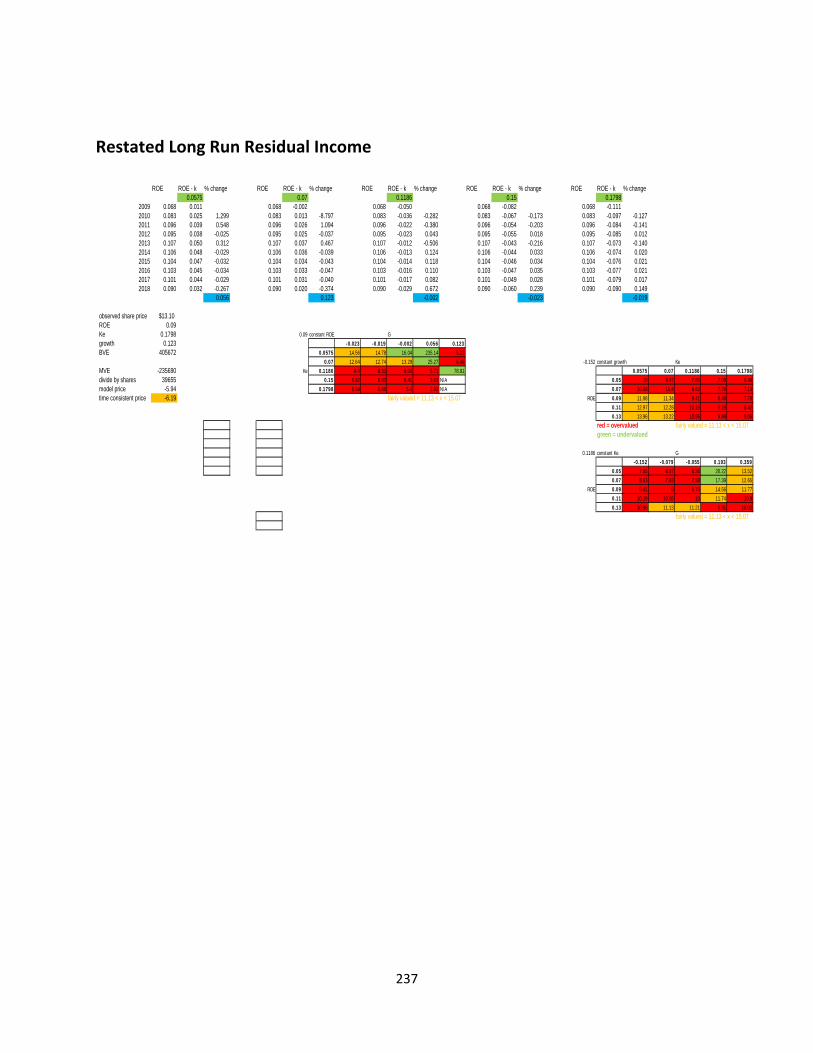
237
Restated Long Run Residual Income
ROE ROE - k % change ROE ROE - k % change ROE ROE - k % change ROE ROE - k % change ROE ROE - k % change0.0575 0.07 0.1186 0.15 0.1798
2009 0.068 0.011 0.068 -0.002 0.068 -0.050 0.068 -0.082 0.068 -0.1112010 0.083 0.025 1.299 0.083 0.013 -8.797 0.083 -0.036 -0.282 0.083 -0.067 -0.173 0.083 -0.097 -0.1272011 0.096 0.039 0.548 0.096 0.026 1.094 0.096 -0.022 -0.380 0.096 -0.054 -0.203 0.096 -0.084 -0.1412012 0.095 0.038 -0.025 0.095 0.025 -0.037 0.095 -0.023 0.043 0.095 -0.055 0.018 0.095 -0.085 0.0122013 0.107 0.050 0.312 0.107 0.037 0.467 0.107 -0.012 -0.506 0.107 -0.043 -0.216 0.107 -0.073 -0.1402014 0.106 0.048 -0.029 0.106 0.036 -0.039 0.106 -0.013 0.124 0.106 -0.044 0.033 0.106 -0.074 0.0202015 0.104 0.047 -0.032 0.104 0.034 -0.043 0.104 -0.014 0.118 0.104 -0.046 0.034 0.104 -0.076 0.0212016 0.103 0.045 -0.034 0.103 0.033 -0.047 0.103 -0.016 0.110 0.103 -0.047 0.035 0.103 -0.077 0.0212017 0.101 0.044 -0.029 0.101 0.031 -0.040 0.101 -0.017 0.082 0.101 -0.049 0.028 0.101 -0.079 0.0172018 0.090 0.032 -0.267 0.090 0.020 -0.374 0.090 -0.029 0.672 0.090 -0.060 0.239 0.090 -0.090 0.149
0.056 0.123 -0.002 -0.023 -0.019
observed share price $13.10ROE 0.09Ke 0.1798 0.09 constant ROE G
growth 0.123 -0.023 -0.019 -0.002 0.056 0.123BVE 405672 0.0575 14.56 14.78 16.04 235.14 5.23
0.07 12.64 12.74 13.29 25.27 6.48 -0.152 constant growth KeMVE -235690 Ke 0.1186 8.4 8.33 8.03 5.71 78.91 0.0575 0.07 0.1186 0.15 0.1798divide by shares 39655 0.15 6.92 6.83 6.41 3.83 N/A 0.05 10 9.47 7.85 7.09 6.49
model price -5.94 0.1798 5.94 5.85 5.4 2.93 N/A 0.07 10.99 10.4 8.63 7.79 7.13
time consistent price -6.19 fairly valued = 11.13 < x < 15.07 ROE 0.09 11.98 11.34 9.41 8.49 7.780.11 12.97 12.28 10.19 9.19 8.420.13 13.96 13.22 10.96 9.89 9.06
red = overvalued fairly valued = 11.13 < x < 15.07green = undervalued
0.1186 constant Ke G-0.152 -0.079 -0.055 0.193 0.359
0.05 7.85 6.87 6.36 20.22 13.520.07 8.63 7.93 7.58 17.39 12.65
ROE 0.09 9.41 9 8.79 14.56 11.770.11 10.19 10.06 10 11.74 10.90.13 10.96 11.13 11.21 8.91 10.02
fairly valued = 11.13 < x < 15.07
238
References
1) Online.wsj.com
2) CFO.com
3) Yahoofinance.com
4) Mergent Online
5) Palepu & Healy
6) Cognex.com
7) Kla-tencor.com
8) Perceptron.com
9) Orbotech.com
10)ESI.com


![[Basque Industry 4.0] Vision Artificial](https://img.pdfslide.net/doc/110x75/55628563d8b42ae73c8b5747/basque-industry-40-vision-artificial.jpg)