Visual ClutterFeature Congestion Model

Cheston Tan6 Nov 2006

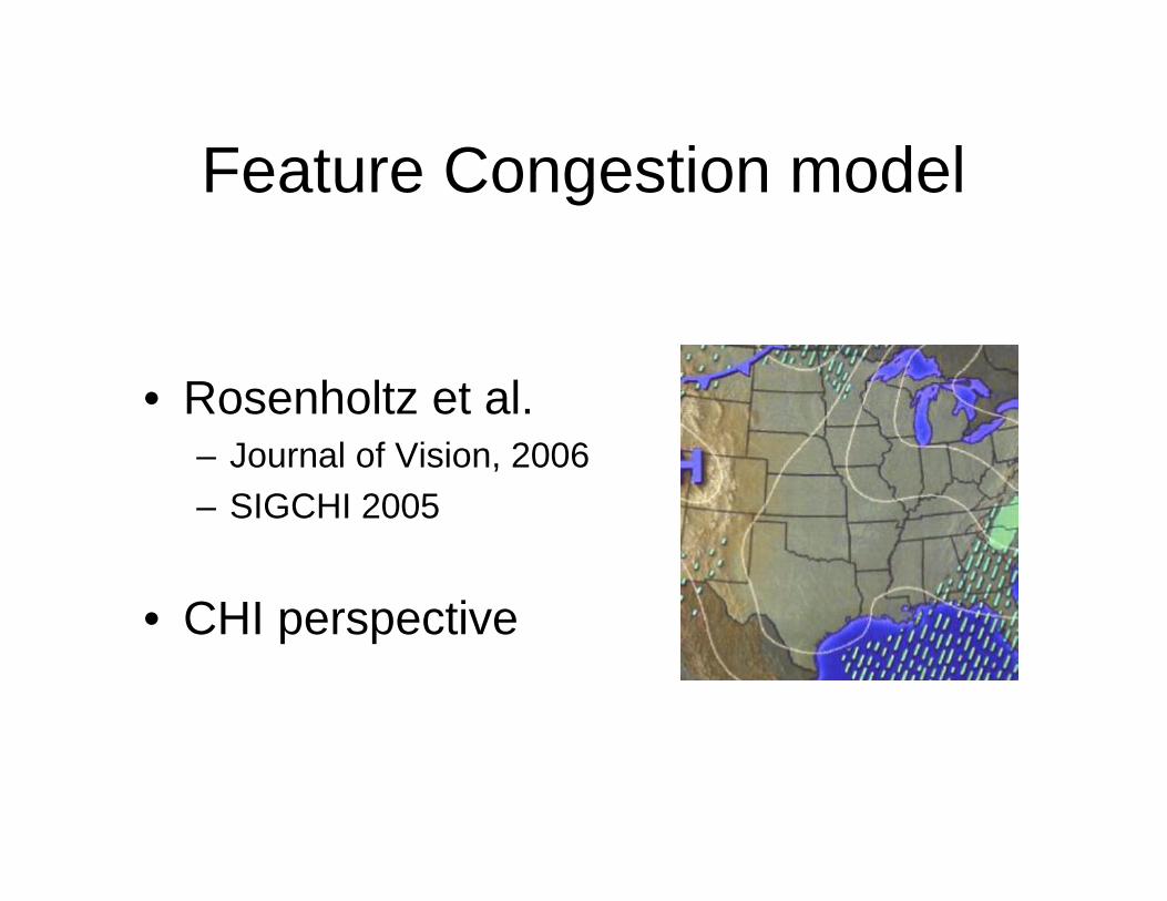
Feature Congestion model

• Rosenholtz et al.– Journal of Vision, 2006– SIGCHI 2005

• CHI perspective

What is “clutter”?

Is clutter subjective?

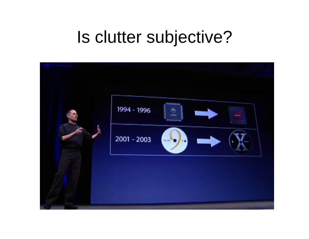
Is clutter subjective?

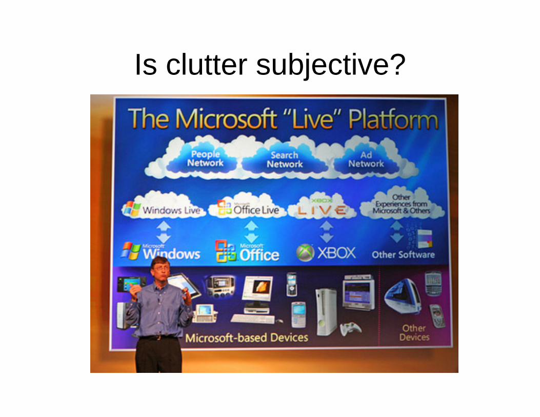
Is clutter subjective?

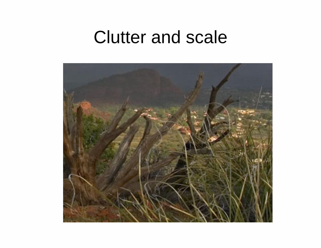
Clutter and scale

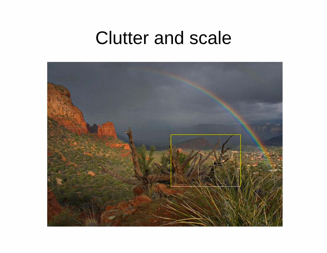
Clutter and scale

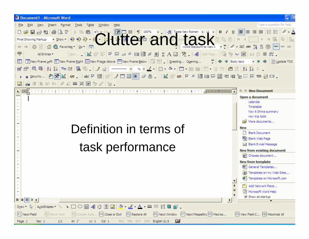
Clutter and task

Definition in terms oftask performance

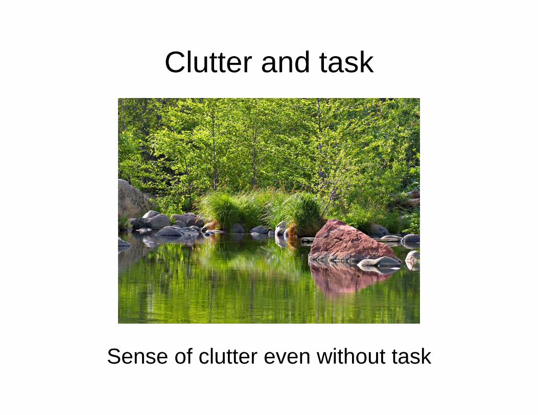
Clutter and task

Sense of clutter even without task

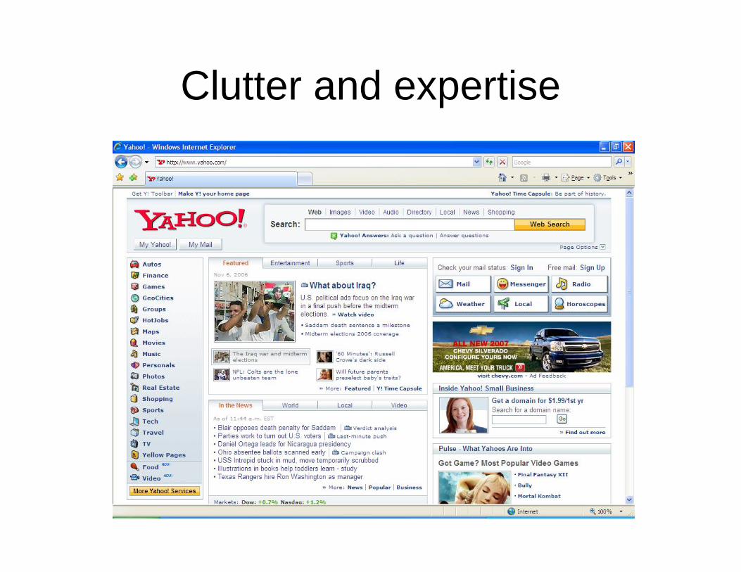
Clutter and expertise

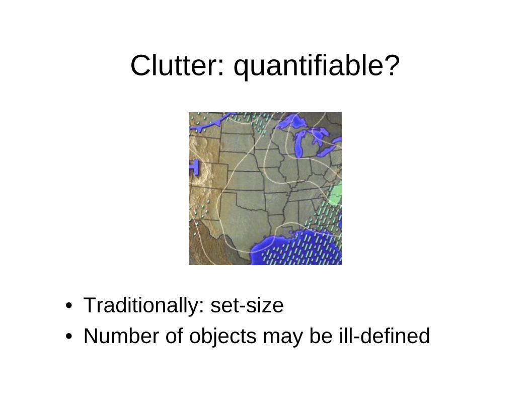
Clutter: quantifiable?

• Traditionally: set-size• Number of objects may be ill-defined

Ways to measure clutter

• Number of visible objects• Number of vertices• Number of elements on webpage• Density of graphics tokens• Number of vectors needed to draw• Length of program• Amount of ink per unit area• Number of bullet points

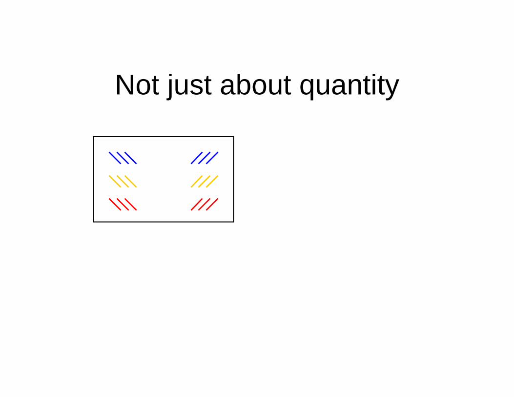
Not just about quantity

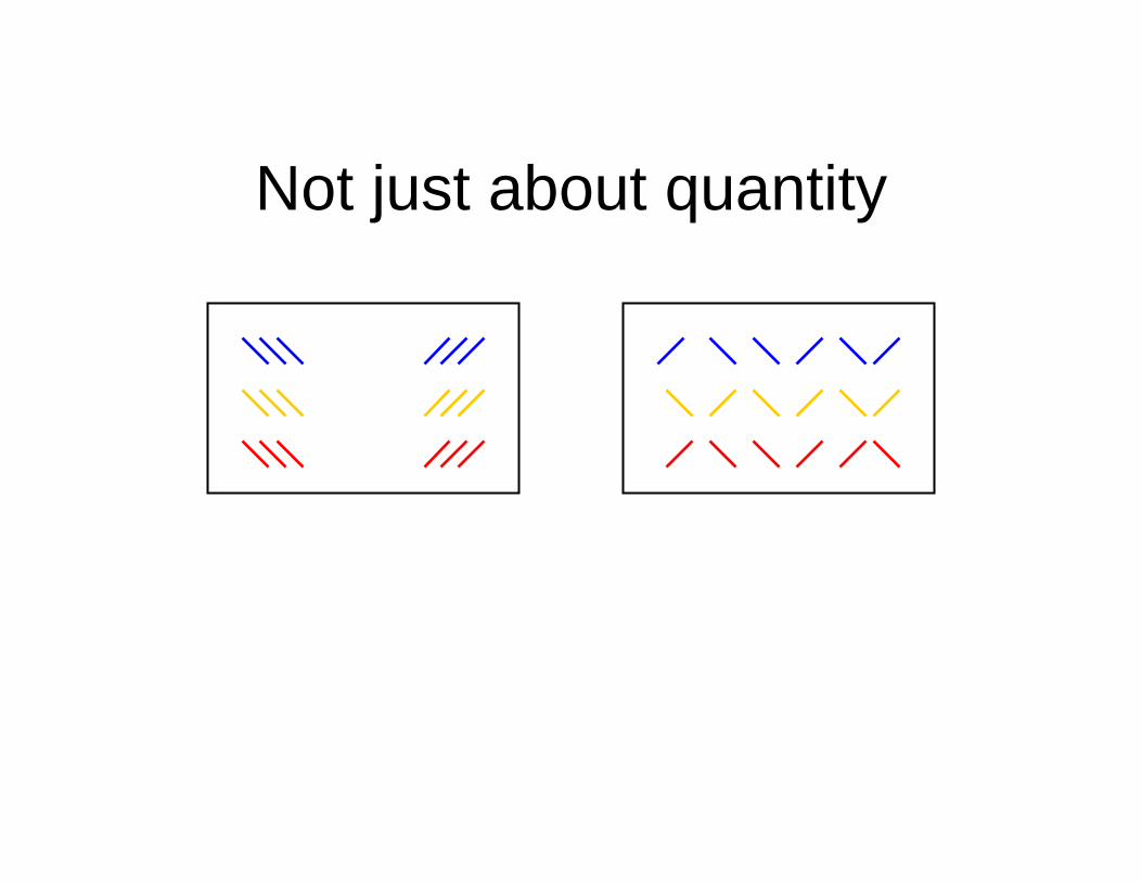
Not just about quantity

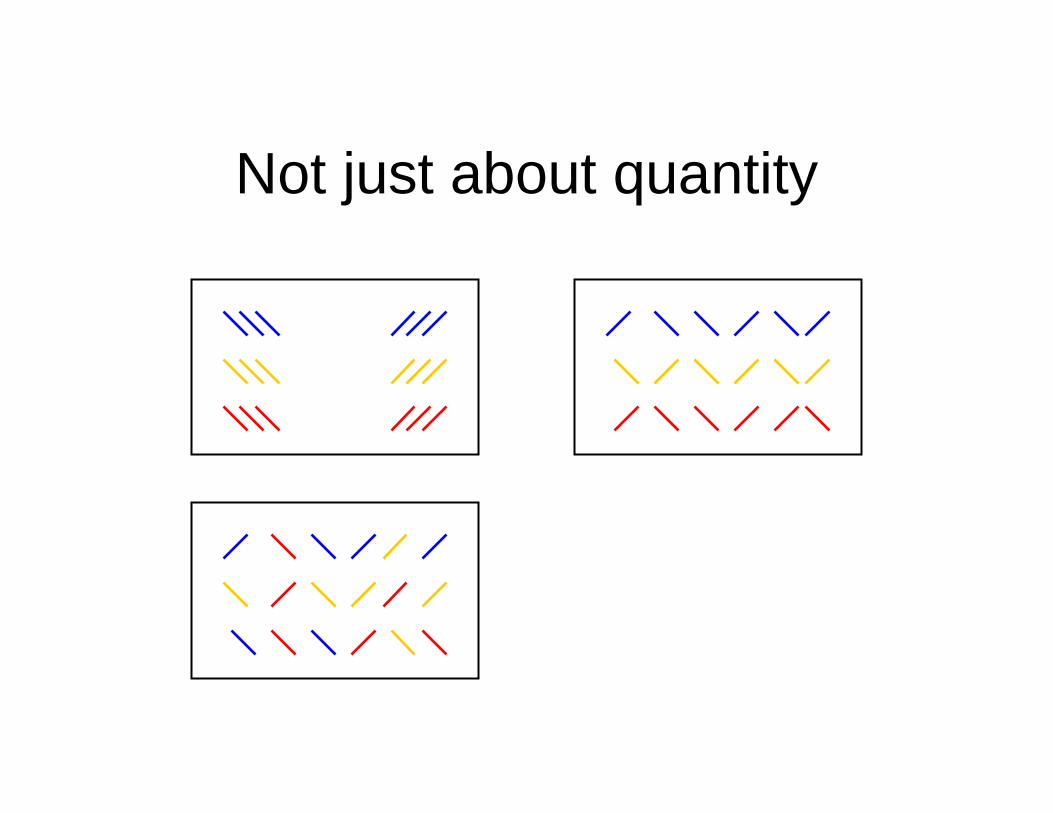
Not just about quantity

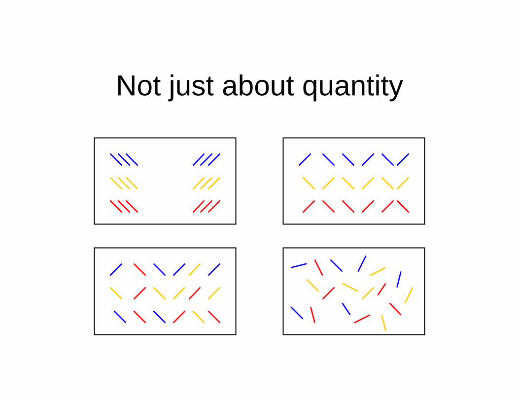
Not just about quantity

Feature Congestion

• Textual definition– “Clutter is the state in which excess items, or their

representation or organization, lead to a degeneration of performance at some task”

• Operational definition– The more cluttered a scene, the more difficult to

add a new item that would draw attention

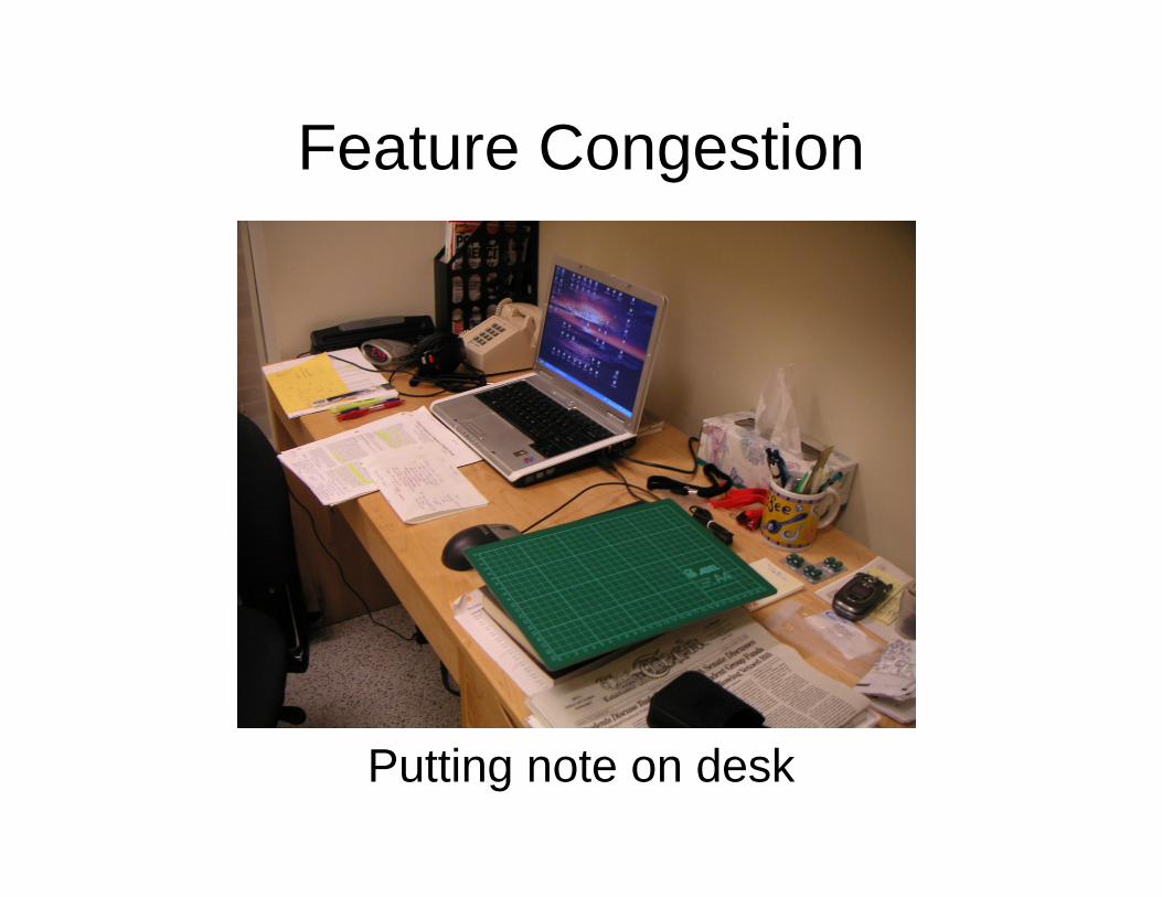
Feature Congestion

Putting note on desk

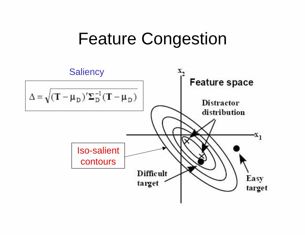
Feature Congestion

Iso-salient contours

Saliency

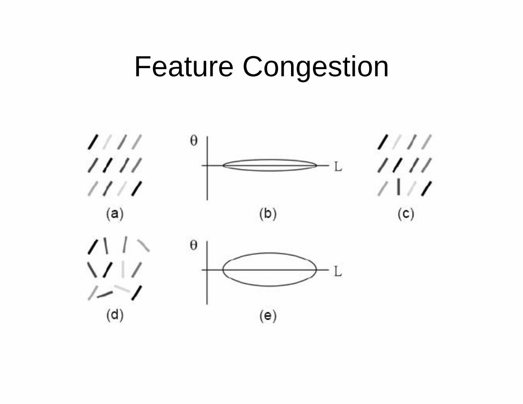
Feature Congestion

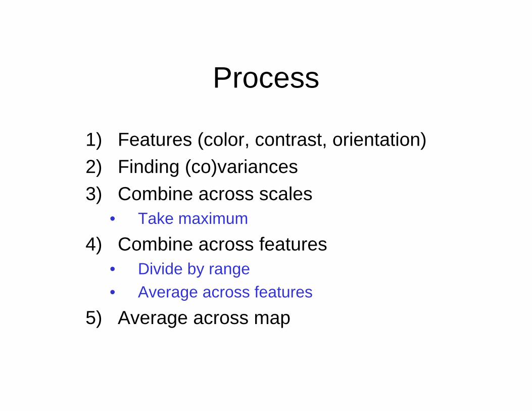
Process

1) Features (color, contrast, orientation)2) Finding (co)variances3) Combine across scales

• Take maximum4) Combine across features

• Divide by range• Average across features

5) Average across map

DEMO

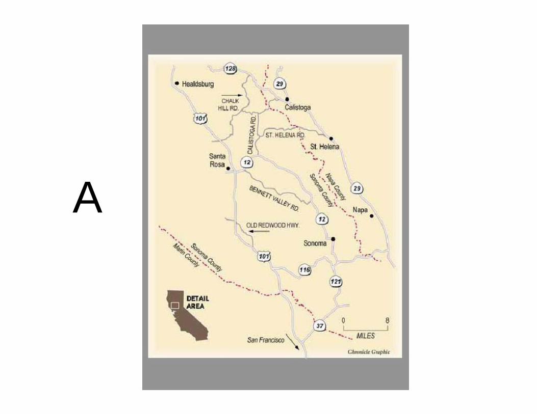
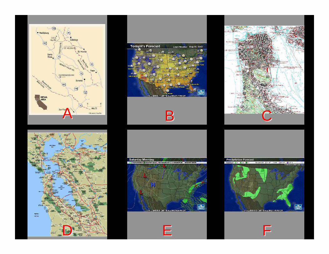
A

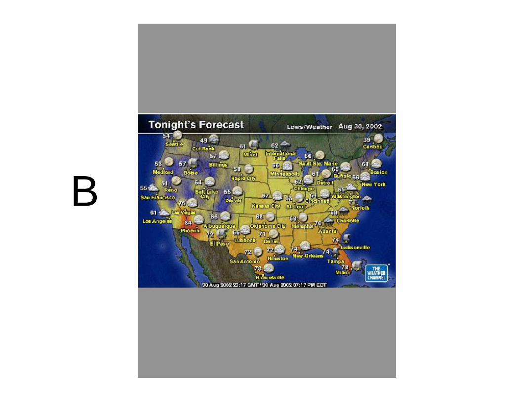
B

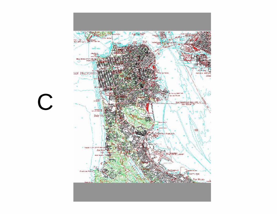
C

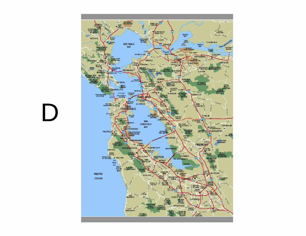
D

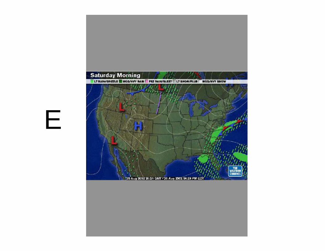
E

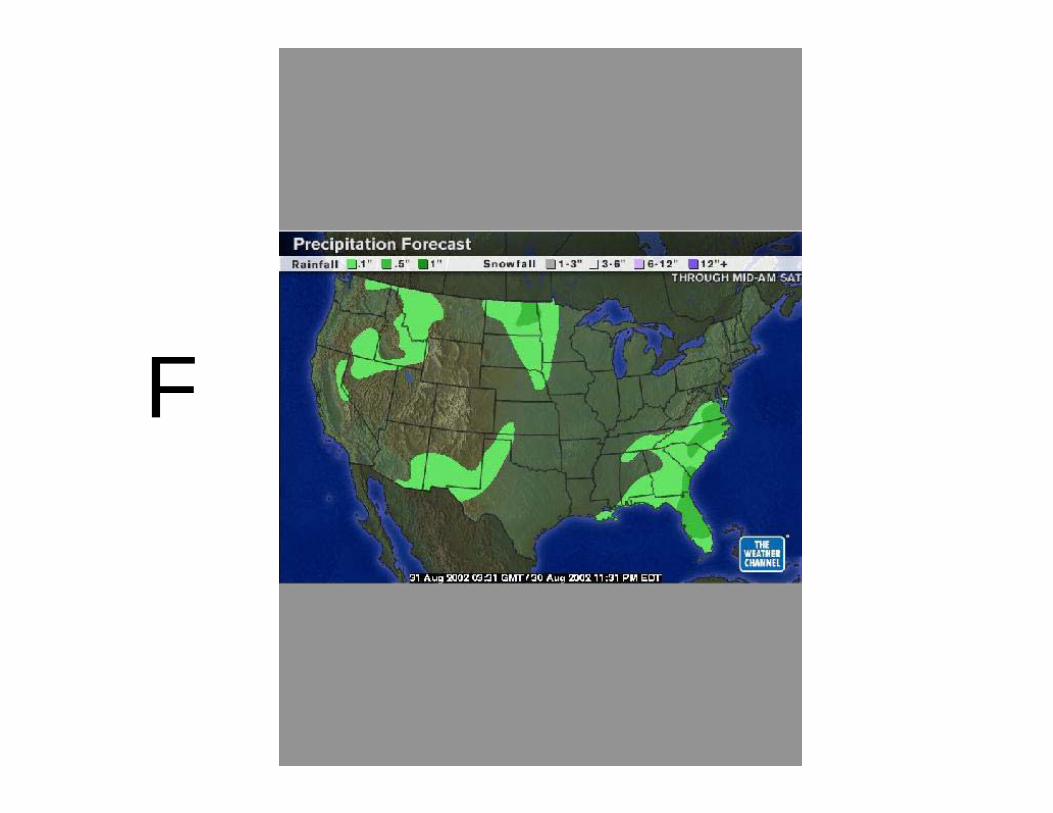
F

AA

DD

BB CC

EE FF

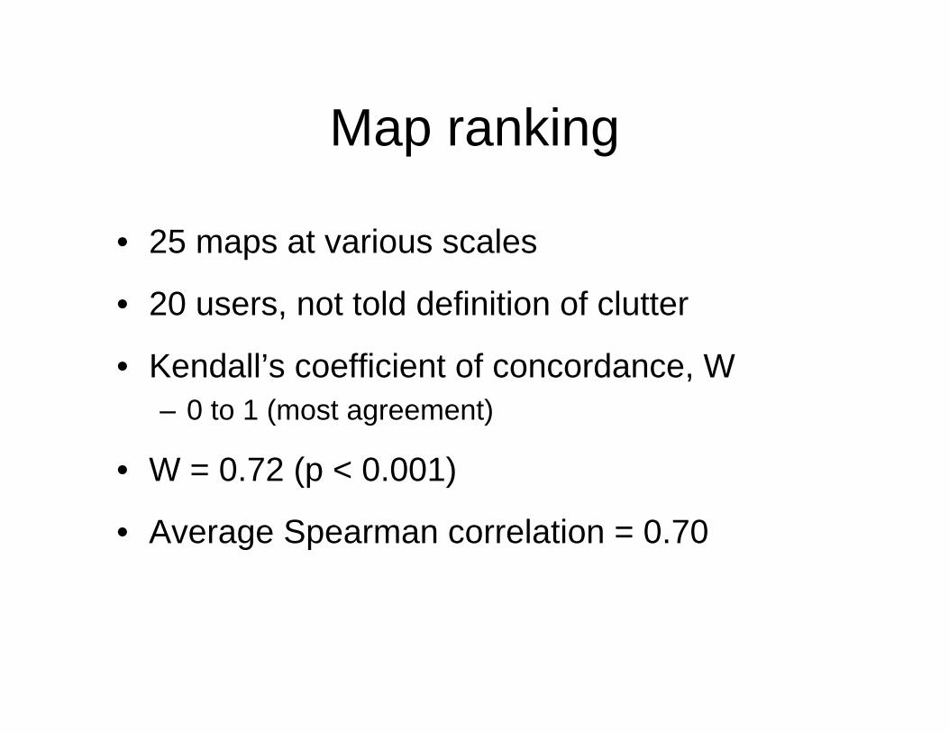
Map ranking

• 25 maps at various scales

• 20 users, not told definition of clutter

• Kendall’s coefficient of concordance, W– 0 to 1 (most agreement)

• W = 0.72 (p < 0.001)

• Average Spearman correlation = 0.70

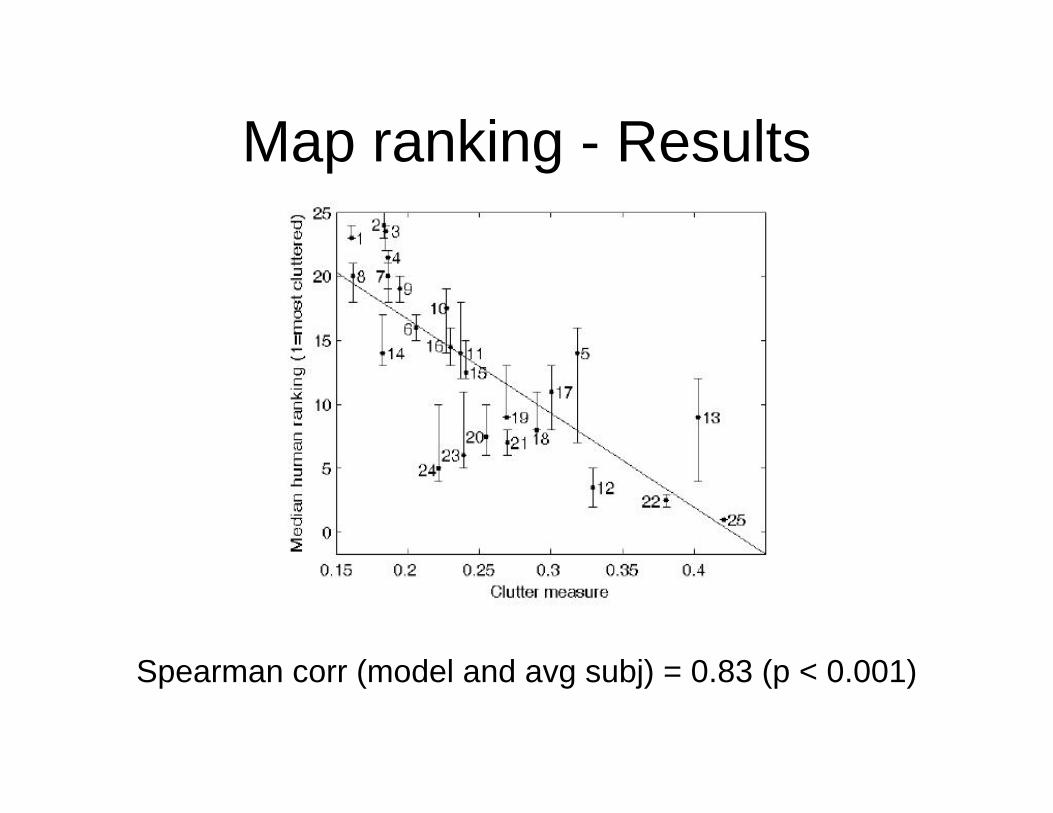
Map ranking - Results

Spearman corr (model and avg subj) = 0.83 (p < 0.001)

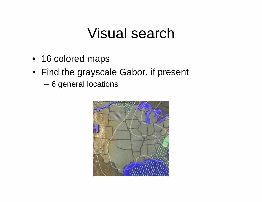
Visual search• 16 colored maps• Find the grayscale Gabor, if present

– 6 general locations

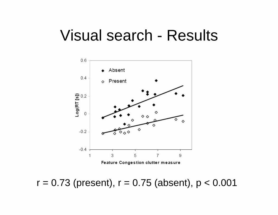
Visual search - Results

r = 0.73 (present), r = 0.75 (absent), p < 0.001

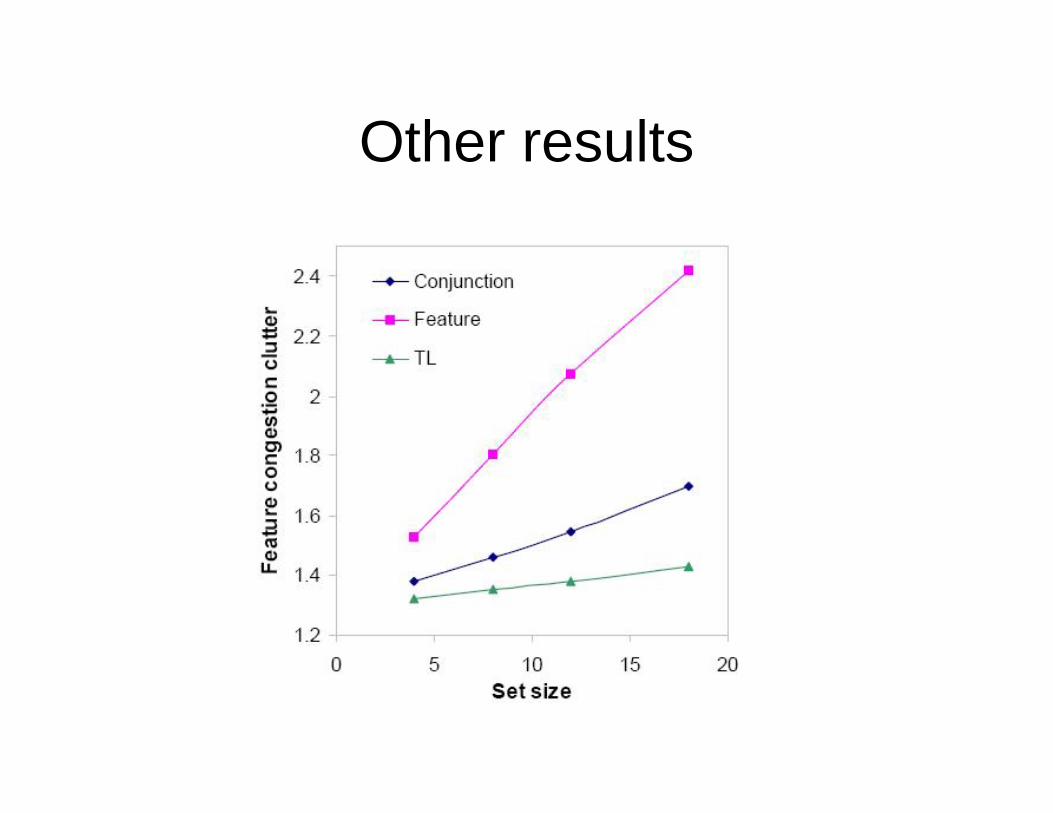
Other results

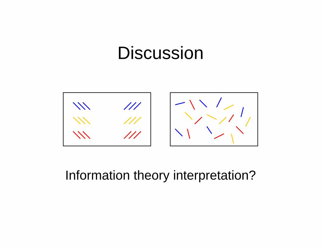
Discussion

Information theory interpretation?

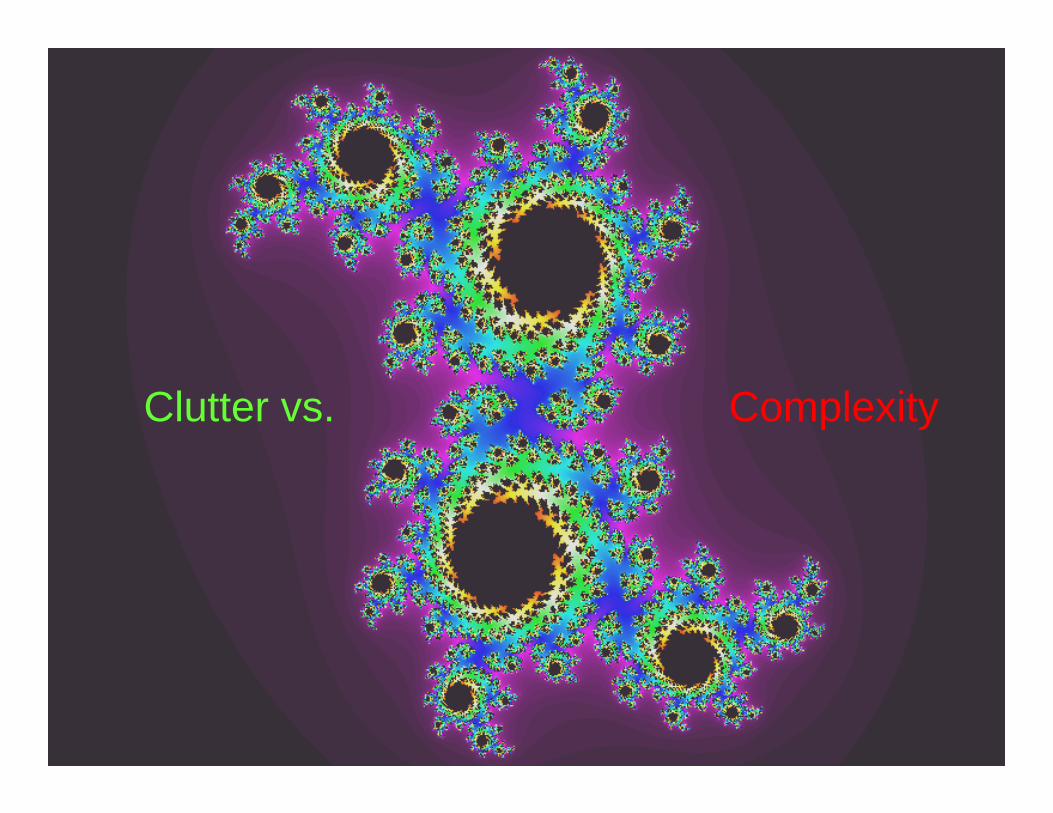
Clutter vs. Complexity

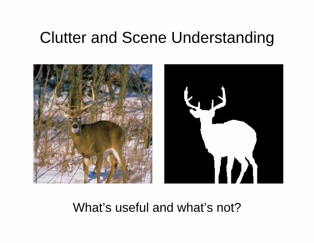
Clutter and Scene Understanding

What’s useful and what’s not?

Sources

• http://presentationzen.blogs.com/• http://www.ipodobserver.com/story/25957• http://www.davidpogue.com/

http://www.youtube.com/watch?v=EUXnJraKM3k