Visual Exploration of Sparse Trafﬁc Trajectory Data · Abstract—In this paper, we present a visual analysis system to explore sparse trafﬁc trajectory data recorded by transportation

Visual Exploration of Sparse Traffic Trajectory Data

Zuchao Wang, Tangzhi Ye, Min Lu, Xiaoru Yuan, Member, IEEE,

Huamin Qu, Member, IEEE, Jacky Yuan and Qianliang Wu

Fig. 1. Our sparse traffic trajectory dataset spans half a year. As shown by the line chart below, the daily traffic flow is rather stable,except during the spring festival. In a snowing morning, the transportation cells are redder, indicating high traffic load. In a springfestival morning, the transportation cells are greener, indicating low traffic load.

Abstract—In this paper, we present a visual analysis system to explore sparse traffic trajectory data recorded by transportation cells.Such data contains the movements of nearly all moving vehicles on the major roads of a city. Therefore it is very suitable for macro-traffic analysis. However, the vehicle movements are recorded only when they pass through the cells. The exact tracks between twoconsecutive cells are unknown. To deal with such uncertainties, we first design a local animation, showing the vehicle movementsonly in the vicinity of cells. Besides, we ignore the micro-behaviors of individual vehicles, and focus on the macro-traffic patterns. Weapply existing trajectory aggregation techniques to the dataset, studying cell status pattern and inter-cell flow pattern. Beyond that,we propose to study the correlation between these two patterns with dynamic graph visualization techniques. It allows us to checkhow traffic congestion on one cell is correlated with traffic flows on neighbouring links, and with route selection in its neighbourhood.Case studies show the effectiveness of our system.

Index Terms—Sparse Traffic Trajectory, Traffic Visualization, Dynamic Graph Visualization, Traffic Congestion

1 INTRODUCTION

Transportation visualizations have been studied for many years. Re-searchers have designed methods to study various kinds of transporta-tion data, including radar based vehicle counting data, taxi GPS data,subway IC card data, etc. Such visualizations help us gain insight intothe complex transportation system.

In this paper, we focus on a new type of transportation data: sparse

• Zuchao Wang is with Peking University. E-mail:

[email protected].

• Tangzhi Ye is with Peking University. E-mail: [email protected].

• Min Lu is with Peking University. E-mail: [email protected].

• Xiaoru Yuan is with Peking University. E-mail: [email protected].

• Huamin Qu is with Hong Kong University of Science and Technology.

E-mail: [email protected].

• Jacky Yuan is with Nanjing Intelligent Transportation Systems Co., Ltd.


• Qianliang Wu is with Nanjing Intelligent Transportation Systems Co., Ltd.


Manuscript received 31 March 2014; accepted 1 August 2014; date of

publication xx xxx 2014; date of current version xx xxx 2014. .

For information on obtaining reprints of this article, please send

e-mail to: [email protected].

traffic trajectory data. Unlike traditional GPS data, our data encom-passes the movements of nearly all vehicles in a city, not just taxis orbuses. Therefore, it can provide accurate traffic statistics, such asflow volume on each cell and between each Origin-Destination (OD).These statistics are very precious in transportation modeling. How-ever, our data is not recorded continuously as in GPS data. Rather, thedata is recorded only when vehicles pass through transportation cells.Therefore, it is spatially sparse, and usually temporally sparse as well.The above differences make our data unique.

To analyse such data, our major challenge is to deal with the uncer-tainties caused by the sparsity. For example, the exact tracks on thelinks between two consecutive cells are unknown. The exact start andend locations of a trajectory are also unknown. Nevertheless, we con-sider movements in the vicinity of cells as of high certainty. Therefore,our first technique is to generate a local animation, which only showsmovements near the cells. Following Andrienko et al.’s work [9], thesecond technique is to aggregate many trajectories, in order to com-pensate for the uncertainties in spatial and temporal coverage. In thisway, we are able to study the cell status patterns (e.g. average speedpattern, congestion pattern) and inter-cell flow patterns.

Beyond studying these patterns separately, we propose to studytheir correlations. That corresponds to interesting domain questionssuch as how traffic congestion on one cell is correlated with traffic

This is the author's version of an article that has been published in this journal. Changes were made to this version by the publisher prior to publication.The final version of record is available at http://dx.doi.org/10.1109/TVCG.2014.2346746

Copyright (c) 2014 IEEE. Personal use is permitted. For any other purposes, permission must be obtained from the IEEE by emailing [email protected].

flows on neighbouring links, and with route selection in its neighbour-hood. To study the correlations, we view the aggregated trajectorydata as a dynamic graph, and apply dynamic graph visualization tech-niques.

The contributions of this work are:

• We present a visual analysis system to explore sparse traffic tra-jectory data, addressing the uncertainties with local animationand trajectory aggregation techniques.

• We study the correlation between cell pattern and link/route flowpattern with dynamic graph visualization techniques.

We will first review related work in Section 2. After that, we givean overview of our system in Section 3, followed by preprocessingin Section 4 and interface design in Section 5. Then we show theeffectiveness of our system with case studies in Section 6. We discussits potentials and limitations in Section 7, and conclude in Section 8.

2 RELATED WORK

Our work is most related to traffic visualization, trajectory visualiza-tion and dynamic graph visualization. Besides, some analytic methodscan be applied to our dataset.

2.1 Traffic Visualization

There are three major types of traffic data: event based, location basedand movement based. Event based traffic data are usually log datacollected manually. Each event usually has position, time and a setof attributes. Location based traffic data are collected by roadsidedetectors, including inductive loops, video cameras, etc. Such dataare mainly used for traffic monitoring at predefined locations. Foreach location, it records a few statistical quantities, e.g. flow volume,occupancy or speed. Movement based traffic data are either directlycollected from GPS devices, or reconstructed from images, videos orpoint clouds. It records the trajectories of a set of vehicles.

In this paper, we focus on sparse traffic trajectory data. It is a com-bination of location based and movement based traffic data, becauseit records the movement of vehicles only at predefined locations. Nosuch traffic data has been studied in the visualization community.

For location based traffic data, Lu et al’s HOMES [29] enables peo-ple to visually summarize inductive loop data in a city at differentlevels. Piringer et al.’s AlVis [33] dealt with video camera data withina tunnel. It is especially designed to enable situational awareness dur-ing emergency events. In above cases, traffic status are visualized ina stand-alone window. Alternatively, it can be embedded into the mapas glyphs [27, 42, 38] for better situational awareness.

Now more and more visualizations are for movement based trafficdata. Various trajectory visualization techniques have been applied.At the local scale, Guo et al. designed TripVista [21] to study micro-traffic patterns at a road intersection. Zeng et al. designed interchangeCircos [45] to study interchange pattern at subway stations. At theglobal scale, Liu et al. designed VAIT [27] to monitor city traffic.Ferreira et al. [20] and Chu et al. [17] studied city taxi datasets.

With our sparse traffic trajectory data, we would mainly explorethe congestion patterns at each cell, and flow patterns at each link androute. Congestion pattern has been studied by Andrienko et al. [5].They extracted traffic congestions from trajectory data, and visualizedthem in map and space time cube. Further, Wang et al. [42] studied thepropagation of traffic congestions along the road network. Link patternhas been studied by Andrienko et al. [7]. They partitioned a city intoregions and studied the traffic flows on the links between neighbouringregions. Route pattern has been studied by Liu et al. [26]. They studiedthe route diversity in a city at different levels. At the bottom level, theycan compare different routes sharing the same origin and destinationin terms of flow volume and attributes. Although each pattern hasbeen studied, there’s no work studying the correlations between thesepatterns. Correlation study is one focus of our paper.

2.2 Trajectory Visualization

Trajectory is a widely studied data type in visualization community. Inthe last two decades, many visual analysis techniques have been devel-oped [3]. According to Andrienko et al.’s paper [4], these techniquescan be categorized into three major types: direct depiction, summa-rization and pattern extraction. All three types of techniques can beapplied to sparse trajectories.

With direct depiction techniques, trajectories are visualized in a di-rect way. That includes representing trajectories as an animation ofmoving objects [31], representing paths as polylines [30] or stackedbands [40], showing temporal information on a timeline [40, 39], andshowing spatial and temporal information together with space timecube [22]. While applying direct depiction techniques to sparse tra-jectories, we need to address the uncertainties in trajectory reconstruc-tion. For example, the exact tracks between two cells are virtuallyunknown, therefore visualizing sparse trajectories with animation andpath polylines assuming linear movement with constant speed can beproblematic. To address such issue, Stoll et al. [37] visualized thereconstruction uncertainties as colored band on top of animation andpath polylines.

With summarization techniques, statistical calculations are per-formed on trajectory data. After that, these statistical summaries in-stead of the trajectories themselves are visualized. Trajectories can besummarized in many ways. Density map [43], spatial temporal aggre-gation [2, 7] and aggregated multivariate glyphs [35] summarize tra-jectories by location, time and attribute. Flow map and flow matrix [2],OD map [44] and Flowstrates [13] summarize trajectories by originand destination. Various clustering algorithms [6, 19] summarize tra-jectories by routes. Andrienko et al. [9] argues that summarizationtechniques are suitable for sparse trajectories, because they reduce theuncertainties in spatial and temporal coverage. Bak et al.’s [11] alsostudied the aggregated patterns of sparse trajectories. In our paper, weapplied summarization techniques. However, we not only study theaggregated patterns separately, but also their correlations.

With pattern extraction techniques, hidden patterns are extractedfrom trajectory data. After that, these patterns are visualized insteadof the trajectories themselves. Typical patterns studied in visualizationcommunity include events [5], moving interactions [8] and movementsemantics [25, 17]. We consider pattern extraction techniques suitablefor sparse trajectories, but we do not study them in this paper.

2.3 Dynamic Graph Visualization

Existing spatial temporal aggregation techniques [2] can transform oursparse traffic trajectory data into flow map. This flow map can be con-sidered as a dynamic graph, with cells as nodes, and inter-cell links asedges. Burch et al. [14] have already tested dynamic graph visualiza-tions on eye tracking trajectories. Therefore, it is natural to also test iton sparse traffic trajectory data.

In their survey, Beck et al. [12] categorized existing dynamic graphvisualization techniques into animation based techniques and time linebased techniques. Animation based techniques visualize data as an an-imation of node-link diagrams [18]. They generally emphasize topo-logical features and are more intuitive. In our paper, we would useanimation to give an overview of city traffic, highlighting the back-bone of the inter-cell links.

Time line based techniques map time to space, usually showingmultiple node-link diagrams [15] or matrices [10] simultaneously.Some techniques integrate node-link diagram and time line in a muchcloser manner. For example, Massive sequence view [41] shows theexistential dynamics of edges, while Flowstrate [13] shows the at-tribute dynamics of edges. Time series glyphs can be associated toeach node [34], showing attribute dynamics of nodes. Shi et al. [36]combined time series glyph and node duplication, transforming dy-namic route selections in a network into a tree style representation.Time line based techniques generally focus on temporal features andare more suitable for analysis. In our paper, we would use time line toanalyze the dynamics of traffic status at each cell, and the dynamics offlow volumes on its related links and routes.



Ahn et al. [1] proposed a taxonomy for dynamic graph analysistasks. They distinguished between low-level tasks and compoundtasks. While low-level tasks are mostly addressed by existing works,compound tasks are not explicitly studied. Two most typical com-pound tasks are inferential task and comparative/correlational task. Inour system, we would explicitly support two correlational tasks, whichanswer interesting domain questions.

2.4 Analytics

Many analytic methods are related to our work. In the trajectory min-ing community, researchers often down-sample vehicle trajectories toroad or region resolution, aggregate them, and then study their gen-eral patterns or extract the outliers. For example, Pang et al. [32]counted the number of taxis in each region of the city at regular timeintervals. Then they detected spatial temporal outliers based on thesecounts. Liu et al. [28] further structured the outlier events into out-lier trees, therefore showing interactions between outliers in neigh-boring regions. In a later work [16], they used L1 optimization toinfer the anomalous routes that cause these outlier events. Althoughabove methods were originally designed for continuous GPS trajecto-ries, skipping the down-sample step, they can be potentially useful toanalyse our sparse traffic trajectory data. More trajectory computationmethods are summarized in Zheng’s book [46]. On the other hand, ifwe first aggregate the trajectories and view it as a dynamic graph, wecan apply network analysis methods. Many of such methods are sum-marized in Kolaczyk et al’s book [24]. These methods can be testedon our data. In this paper, we focus on visualization. Therefore wehave not implemented these analytic methods, except for the minDis-tort algorithm [28] for abnormality calculation in each cell. However,we consider them complementary to our work, and would implementthem if necessary.

3 OVERVIEW

In this section, we first describe the data we use. After that, we explainour design considerations and present the pipeline of our system.

3.1 Data Description

In the past few years, government in the city of Nanjing, China hasbeen pushing a project on intelligent transportation system. In thisproject, several hundreds of transportation cells are set up on the road-side for traffic monitoring. The cells are usually installed at approx.200 meters downstream a road intersection. Each cell is directed,meaning it is responsible for only one-direction of traffic flow. Thecells have video cameras mounted in order to record vehicles passingthrough.

Our dataset contains two parts: trajectory data and celldata. The trajectory data are derived from the video cam-eras, in which vehicles are extracted from video streams, andidentified via license plate recognition techniques. Basically,it contains a list of vehicle passing records, each correspond-ing to one vehicle passing through one cell. The data formatis 〈plate number, plate color,cell id, lane id,speed, timestamp〉. Avehicle can be uniquely identified with its plate number plusplate color. For the cell data, it contains the names, spatial positionsand directions of the transportation cells.

Our trajectory data spans 169 consecutive days, from Sep. 22nd2012 to Mar. 9th 2013. The daily record number is shown in the linechart of Figure 1. All together there are 870 million records, with over1 million vehicles. The data size is 39 GB. Besides, in the cell data,472 cells are recorded.

Before visual design, we have made some preliminary analysis onthe trajectory data of one day. We chose Dec 1.st, 2012. This was aSaturday, which contains 5,177,062 records. Figure 2 plots the posi-tions of the cells. For each cell, we calculate its traffic flow volume asthe number of records in trajectory data. This is mapped to the circlesize on the map. A picture of the busiest cell is shown in the inset ofthis figure. As Figure 3(a) illustrates, on this day, one cell can have0 to 100,000 records, with the average number being 14,000. Thereare 108 cells with less than 1000 records, 98 of which have 0 record.

Fig. 2. Locations of all transportation cells in Nanjing. Each circle rep-resents one cell, with its area being proportional to flow volume on Dec.1st, 2012. A picture of the busiest cell is shown in the inset.

These cells may be obsolete, malfunctioned or under construction. AsFigure 3(b) shows, the mean speed in this day is around 30 km/h. Wecan see that the main body of the speed distribution seems to obey aGaussian distribution. Besides, there are two outlier peaks at 0 km/hand 10 km/h. This distribution also has a long tail, with maximumspeed being 500 km/h.

0 20000 40000 60000 80000 100000

Number of cell records (bin size = 1000)

0

20

40

60

80

100

120

Nu

mb

er

of

cells

Record Number Distribution for All Cells

(a)

0 20 40 60 80 100 120

Vehcile speed (bin size = 1 km/h)

0

1e+5

2e+5

3e+5

4e+5

5e+5

6e+5

7e+5

Nu

mb

er

of

reco

rds Vehicle Speed Distribution for All Records

(b)

Fig. 3. Statistics of all cells in Nanjing, on Dec. 1st, 2012. (a) Thedistribution of record number in each cell. (b) The distribution of vehiclespeeds in all cells.

We further focus on that busiest cell. Figure 4(a) shows its trafficflow in this day. We can see that the flow volume reached a high levelat 8 am, and kept high until 4 pm. The maximum traffic flow per 10minutes is 1174, at 9:50 am. From Figure 4(b), we can see the trafficspeed began to drop at 7 am, and began to recover at 6 pm. At noon,there’s a small increase of traffic speed, but it dropped back quickly.



00:00 03:00 06:00 09:00 12:00 15:00 18:00 21:00 00:00

Time (bin size = 10 minutes)

0

200

400

600

800

1000

1200Tr

aff

ic f

low

vo

lum

e One Cell Traffic Flow

(a)

00:00 03:00 06:00 09:00 12:00 15:00 18:00 21:00 00:00

Time

0

20

40

60

80

100

120

Traff

ic s

peed

(km

/h) One Cell Traffic Speed

(b)

Fig. 4. Traffic condition of one cell in Nanjing, on Dec. 1st, 2012. Thiscell is highlighted in Figure 2. (a) One day traffic flow. (b) One daytraffic speed, where each black dot is a record in the trajectory data,with y position representing speed value. The red line is a LOWESSsmoothing of these speed values.

3.2 Design Considerations

We compare our cell-based sparse trajectory data with taxi GPS tra-jectory data. Their differences are summarized below:

• Sparse in terms of location: In our data, vehicle movementsare recorded only when they pass through one of the cells. Theexact start/end locations and the tracks between two consecutivecells are uncertain. This spatial sparsity also results in temporalsparsity. In contrast, in taxi GPS trajectory data, movements arerecorded in a quasi-continuous manner.

• Dense in terms of population: In our data, vehicles are sampledvery densely. It covers almost all vehicles running on the majorroads of Nanjing. In contrast, GPS data are usually restricted totaxis, which are just a small subset of vehicles.

• Accurate traffic flow volume: Because of the dense samplingin population, traffic flow volume can be calculated accurately.It is usually not possible with taxi GPS data.

• Accurate traffic speed: Traffic speed can be estimated at highaccuracy. In contrast, estimation based on taxi GPS data canbe biased, because taxi drivers sometimes drive in low speed tosearch for passengers.

• Suitable for network analysis: Network analysis can be per-formed more accurately, due to accurate estimations of flow vol-ume and speed. However, this can be problematic with taxi GPSdata.

• Not suitable for vehicle tracking: Vehicles can not be trackedaccurately all over the map, because their positions are onlyrecorded at the cells. However, in taxi GPS data, vehicles canbe tracked in high precision, with the help of map matching al-gorithms.

Although our data is sparse in terms of location and time, it still hasmuch richer information than the OD data. When using OD data, onlyorigin and destination location/time are known. It is impossible to getaccurate traffic flow volume and speed information at each location,on each link and along each route. As a result, many network analysistasks can not be performed. Vehicle tracking now becomes impossible,even locally.

In conclusion, compared with traditional GPS data and OD data,our sparse traffic trajectory data can give much more accurate trafficstatistics, and therefore is the ideal data for network analysis. How-ever, we have to consider the uncertainties.

Regarding the uncertainties, we make use of two techniques. Thefirst technique is local animation. We believe showing an intuitive an-imation of vehicle movements is important in data exploration. How-ever, due to spatial and temporal sparsity, we can not accurately trackthe vehicles. In our data, vehicles move on the complex city roadnetwork. Their start/end locations, route selection and travel speedbetween consecutive cells are all unknown. A reasonable trajectoryreconstruction is very difficult. Therefore, we only reconstruct themovements in the vicinity of cells, where we believe the movementsare of high certainty. Then we visualized such local tracking with localanimation.

Following Andrienko et al.’s work [9], the second technique is toaggregate many trajectories, in order to compensate for the uncertain-ties in spatial and temporal coverage. In this way, we transform ourdata into flow map, which is essentially a dynamic graph. Therefore,we can perform network analysis to study the macro-traffic patterns.

According to Kelly’s formalization [23], traffic flow can be mod-eled mathematically, as illustrated on the left of Figure 5. There areseveral core concepts in this model: node, link, route and OD. In ourcase, each cell Ci is a node. If vehicle moves from cell C0 directly tocell C1, without passing any intermediate cells, then C0 → C1 formsa link. Each cell is connected to multiple links. Some are upstreamlinks which end at this cell, while some are downstream links whichstart from this cell. A series of links C0 → C1 → ... → CN forms aroute. The start and end cells of a route forms an Origin Destinationpair (abbrev. as OD), e.g. C0 ⇒CN . Each route consists of a sequenceof links, and a link can be shared by multiple routes. Each route cor-responds to one OD, and for one OD there can be multiple routes.

Our network analysis consists of three steps, as shown on the rightof Figure 5. Basically, users first get an overview of the traffic status atcity scale. In this process, they find some cells interesting, select themand examine their local traffic patterns. Once they discover traffic con-gestions or abnormalities on a specific cell, they can check whetherthey are correlated with flow patterns on its upstream/downstreamlinks or vehicles’ route selection. The three exploration steps are de-tailed below:

• Global Exploration focuses on presenting an intuitive overviewof the city traffic. Users can check the traffic status of all cellsand the flow volumes on major links at a specific time. Con-gested cells and backbone links can be discovered.

• Cell Exploration focuses on revealing the traffic patterns at eachcell. Users can select one central cell each time. They checkhow its traffic speed and flow volume change with time, and tryto discover trend and periodicity. Users can also see when trafficcongestions occur on the central cell, and when the traffic statuslooks abnormal. Users can partly reproduce the traffic scenariowith local animation.

• Correlation Exploration focuses on testing correlations be-tween cell patterns and link/route patterns. That corresponds tointeresting domain questions such as how traffic congestion onone cell is correlated with traffic flows on neighbouring links,and with route selection in its neighbourhood. Given a centralcell, users first select its major upstream/upstream links. Thenthey check which of these links have an increasing or decreasingflow volume when the central cell starts getting congested. Al-ternatively, users can select a route passing by the central cell.Then users check whether the flow volumes on this route andits alternative routes increase or decrease when the central cellstarts getting congested. If correlation is detected, users can tryto explain it by searching for news on the Internet.



Data Model

Node

Link

Route

Origin/Destination

Global Exploration

Cell Exploration

Examination of local traffic status at each

cell

Overview of traffic status at city scale

Exploration Model

Upstream Link

Downstream Link

Correlation ExplorationDiscovery of correlations between cell

status and flow patterns on links/routes

Fig. 5. Conceptual model of our network analysis: based on a formalnetwork data model, we propose three exploration steps: global explo-ration, cell exploration and correlation exploration.

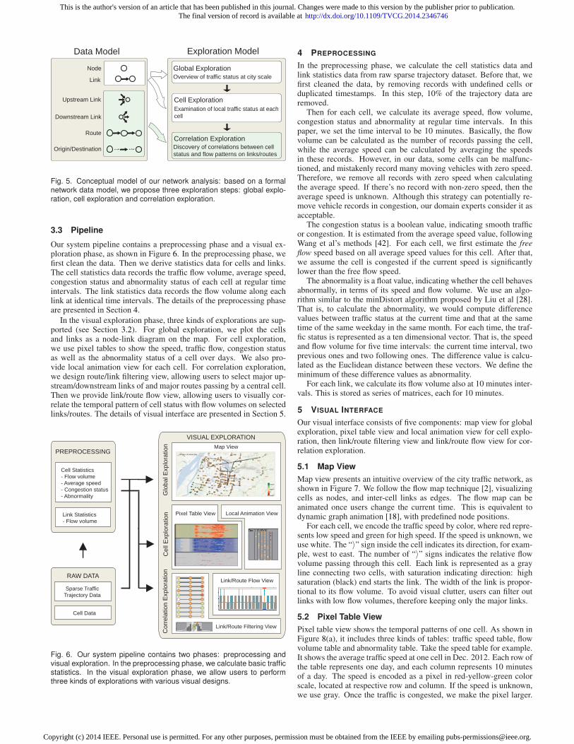
3.3 Pipeline

Our system pipeline contains a preprocessing phase and a visual ex-ploration phase, as shown in Figure 6. In the preprocessing phase, wefirst clean the data. Then we derive statistics data for cells and links.The cell statistics data records the traffic flow volume, average speed,congestion status and abnormality status of each cell at regular timeintervals. The link statistics data records the flow volume along eachlink at identical time intervals. The details of the preprocessing phaseare presented in Section 4.

In the visual exploration phase, three kinds of explorations are sup-ported (see Section 3.2). For global exploration, we plot the cellsand links as a node-link diagram on the map. For cell exploration,we use pixel tables to show the speed, traffic flow, congestion statusas well as the abnormality status of a cell over days. We also pro-vide local animation view for each cell. For correlation exploration,we design route/link filtering view, allowing users to select major up-stream/downstream links of and major routes passing by a central cell.Then we provide link/route flow view, allowing users to visually cor-relate the temporal pattern of cell status with flow volumes on selectedlinks/routes. The details of visual interface are presented in Section 5.

VISUAL EXPLORATION

Map View

Glo

bal E

xplo

ration

Corr

ela

tion E

xplo

ration

Cell

Explo

ration

RAW DATA

Sparse Traffic

Trajectory Data

Cell Data

PREPROCESSING

Cell Statistics

- Flow volume

- Average speed

- Congestion status

- Abnormality

Local Animation ViewPixel Table View

Link/Route Flow View

Link/Route Filtering View

Link Statistics

- Flow volume

Fig. 6. Our system pipeline contains two phases: preprocessing andvisual exploration. In the preprocessing phase, we calculate basic trafficstatistics. In the visual exploration phase, we allow users to performthree kinds of explorations with various visual designs.

4 PREPROCESSING

In the preprocessing phase, we calculate the cell statistics data andlink statistics data from raw sparse trajectory dataset. Before that, wefirst cleaned the data, by removing records with undefined cells orduplicated timestamps. In this step, 10% of the trajectory data areremoved.

Then for each cell, we calculate its average speed, flow volume,congestion status and abnormality at regular time intervals. In thispaper, we set the time interval to be 10 minutes. Basically, the flowvolume can be calculated as the number of records passing the cell,while the average speed can be calculated by averaging the speedsin these records. However, in our data, some cells can be malfunc-tioned, and mistakenly record many moving vehicles with zero speed.Therefore, we remove all records with zero speed when calculatingthe average speed. If there’s no record with non-zero speed, then theaverage speed is unknown. Although this strategy can potentially re-move vehicle records in congestion, our domain experts consider it asacceptable.

The congestion status is a boolean value, indicating smooth trafficor congestion. It is estimated from the average speed value, followingWang et al’s methods [42]. For each cell, we first estimate the freeflow speed based on all average speed values for this cell. After that,we assume the cell is congested if the current speed is significantlylower than the free flow speed.

The abnormality is a float value, indicating whether the cell behavesabnormally, in terms of its speed and flow volume. We use an algo-rithm similar to the minDistort algorithm proposed by Liu et al [28].That is, to calculate the abnormality, we would compute differencevalues between traffic status at the current time and that at the sametime of the same weekday in the same month. For each time, the traf-fic status is represented as a ten dimensional vector. That is, the speedand flow volume for five time intervals: the current time interval, twoprevious ones and two following ones. The difference value is calcu-lated as the Euclidean distance between these vectors. We define theminimum of these difference values as abnormality.

For each link, we calculate its flow volume also at 10 minutes inter-vals. This is stored as series of matrices, each for 10 minutes.

5 VISUAL INTERFACE

Our visual interface consists of five components: map view for globalexploration, pixel table view and local animation view for cell explo-ration, then link/route filtering view and link/route flow view for cor-relation exploration.

5.1 Map View

Map view presents an intuitive overview of the city traffic network, asshown in Figure 7. We follow the flow map technique [2], visualizingcells as nodes, and inter-cell links as edges. The flow map can beanimated once users change the current time. This is equivalent todynamic graph animation [18], with predefined node positions.

For each cell, we encode the traffic speed by color, where red repre-sents low speed and green for high speed. If the speed is unknown, weuse white. The “〉” sign inside the cell indicates its direction, for exam-ple, west to east. The number of “〉” signs indicates the relative flowvolume passing through this cell. Each link is represented as a grayline connecting two cells, with saturation indicating direction: highsaturation (black) end starts the link. The width of the link is propor-tional to its flow volume. To avoid visual clutter, users can filter outlinks with low flow volumes, therefore keeping only the major links.

5.2 Pixel Table View

Pixel table view shows the temporal patterns of one cell. As shown inFigure 8(a), it includes three kinds of tables: traffic speed table, flowvolume table and abnormality table. Take the speed table for example.It shows the average traffic speed at one cell in Dec. 2012. Each row ofthe table represents one day, and each column represents 10 minutesof a day. The speed is encoded as a pixel in red-yellow-green colorscale, located at respective row and column. If the speed is unknown,we use gray. Once the traffic is congested, we make the pixel larger.



Average Speed

Flow Volume

& Direction

Fig. 7. Map view: overview of city traffic network, visualizing cells asnodes, and inter-cell links as edges. To avoid visual clutter, only linkswith 10-minutes flow volumes above 100 are shown.

This table like design helps summarize daily traffic pattern, and hasproven effective in Wang et al.’s work [42]. In our system, we allowusers to switch on/off each of the three tables. We further allow usersto make periodic filtering. For example, in Figure 8(b), we only showthe traffic status during the daytime of weekends.

5.3 Local Animation View

In addition to pixel tables, we also design local animation view forcell exploration. We believe an intuitive animation will be importantin giving users a first impression of the data. It can also help vali-date discoveries made by statistic or data mining methods, as shownin Wang et al.’s work [42]. However, as mentioned in Section 3.2, tra-ditional animation is not applicable due to the uncertainties caused bysparsity. Therefore, we only reconstruct the traffic within 200 meterinterval downstream of each cell. In the reconstruction, we assume thatthe vehicles move with constant speed and never change lanes. Thenwe are able to show a local animation, as in Figure 8(c). In the localanimation view, we draw black lines to separate the lanes, and dots toshow the vehicles. The dot color represents the speed of vehicle.

(a)

(b) (c)

Speed

Flo

w V

olu

me

Abm

orm

alit

y

Fig. 8. (a) Pixel table view shows the temporal patterns of one cell,including traffic speed, flow volume, abnormality and congestion statusin Dec. 2012. (b) Pixel table supports periodic filtering. This table showsthe traffic status during the daytime of weekends. (c) Local animationview shows the traffic animation at one cell.

5.4 Link/Route Filtering View

Given a central cell, the first step of correlation exploration is to selectits related links/routes. This is supported by link/route filtering view.

Link filtering view supports the selection of most related up-stream/downstream links, as shown in Figure 9(a). It consists of twohistograms. Given the central cell, the left histogram displays the topten highest flow volumes of its upstream links, while the right his-togram is for downstream links. Users can select links directly onthese histograms, for example, the top three upstream links and topfive downstream links. Selected links are highlighted on the map, withtheir width proportional to the flow volumes at the current time. Wecan color these links in gray, identical to that in the map view. How-ever, in order to show whether the flow volume is increasing or de-creasing, now we prefer to color them in a yellow-gray-blue colorscale, as shown in Figure 10. Yellow indicates decreasing flow vol-umes, while blue indicates increasing flow volumes. Again, saturationindicates direction, with high saturation end starting the link.

Route filtering view supports the selection of related routes. Thatincludes one central route R passing the central cell, and route R’smultiple alternative routes. For simplification, in our system we onlyconsider routes consisting of three cells. So the central route R is inthe form Cstart → Ccentral → Cend , where Ccentral is the central cell.Cstart and Cend are the start and end cells of the route. The alterna-tive routes of R share the same OD Cstart ⇒ Cend with R. However,they bypass the central cell, so each alternative route is in the formCstart → Calternative → Cend , where Calternative is a cell different fromthe central cell Ccentral . Our system first tries to recommend the centralroute R. As shown in Figure 9(b), our system would choose the top tenroutes passing the central cell with highest flow volumes. These tenroutes are arranged vertically and aligned horizontally. For each route,we have three circles. From left to right, they represent the start cell,central cell and end cell. The cell color indicates its traffic speed at thecurrent time. Two lines connecting the circles represent links betweencells. The width of the line is proportional to the flow volume on routeR. Each line also has a gray background, whose width is proportionalto the total flow volume on the link. This gives some contextual infor-mation. As we consider routes with high flow volumes more relevantto the central cell, we suggest users to choose route R with thick blacklines, which are arranged on top. Once users select route R, its topten alternative routes with highest flow volumes will be automaticallyselected. On the map, the central route R will be highlighted, with an“S” sign besides the start cell, and an “E” sign besides the end cell.However, the alternative routes will not be highlighted automatically.Users can highlight them manually on the route flow view, which willbe mentioned later.

Recommended

Central Routes

Recommended

Central Routes

Start

Cell

Central

Cell

End

Cell

(a) (b)

Fig. 9. (a) Link filtering view supports the selection of major up-stream/downstream links of the central cell. These links will be usedfor cell-link correlation discovery. (a) Route filtering view supports theselection of one route passing the central cell, and its alternative routes.These routes will be used for cell-route correlation discovery.



5.5 Link/Route Flow View

After filtering the related links and routes, users try to discover thecorrelation between cell status pattern and link/route pattern. That issupported by link/route flow view.

With link flow view, we compare flow volumes on links, and cor-relate them with traffic status on the central cell. This would be adynamic graph exploration task. Among various visualization tech-niques for dynamic graph, we think Flowstrates [13] will be a goodstarting point for our design. It is a time line based method speciallydesigned to compare temporal patterns on links. As shown in Fig-ure 10, the link flow view has a horizontal time axis. In the middle ofthis view, it’s the link region, showing the flow volumes of four linkson four rows. Their names are labelled on the left, in Chinese charac-ter. At each time interval, the flow volume of each link is representedas a rectangle. Instead of purely using color encodings in Flowstrates,we use both color and width of rectangle. This is because we want toshow two properties simultaneously. We use the width of rectangle toencode the magnitude of flow volume, and color to encode its increas-ing/decreasing rate. The color scale is yellow-gray-blue, identical tothat used in the link/route filtering view: yellow for decreasing andblue for increasing. The upstream links are drawn at the lower half ofthe link region, while the downstream links at the upper half. Then theupstream links and downstream links are ordered by total flow volumeseparately. On top of the link region is the cell speed band, where weshow the speed pattern of the central cell. Below the link region is thecell flow band, where we show the flow volume pattern of the centralcell. At some time interval, the band appears larger than usual. Thatindicates traffic congestion. These two bands are aligned with the linkregion, enabling visual correlation of cell status pattern and link flowpatterns.

The route flow view reuses the above design, but shows cell-routecorrelation instead of cell-link correlation. The only difference in ourdesign is that now the central link region becomes the route region,where each row represents one route. One of these routes will be thecentral route R. It passes through the central cell. Others are the al-ternative routes of R. These routes are vertically ordered by total flowvolume.

Cell Speed

Band

Cell Flow

Band

Link Region

Name of LinkDecreasing Increasing

Fig. 10. Link flow view supports visual comparison among flow patternson upstream/downstream links of a central cell, and visual correlationbetween those flow patterns and traffic status on the central cell.

6 CASE STUDIES

In this section, we present four studies, demonstrating the three kindsof explorations supported by our system. The first case is for globalexploration, the second for cell exploration, while the last two casesare for correlation exploration.

6.1 Case 1: City Traffic Network Exploration

In this case, we study the city level traffic condition. We choose fourtypical times on Dec. 1st, 2012, and compare the network patterns atthose times. In Figure 11, we can see that the traffic during morningpeak and evening peak are very different. At 8 am in the morning,the traffic is relatively smooth at all cells. There are many high flowvolume links, indicating the traffic load is high. However, at 6 pmin the evening, the traffic is rather congested at all cells. At the meantime, there are much fewer high flow volume links. It perhaps indicatesthat traffic flow drops due to congestions during the evening peak.

From the figures, we can clearly see the backbone of Nanjing’s traf-fic. Position A seems to be the most important hub. It is the railwaystation in Nanjing. Major traffic routes in the city are between A and B,

A and C, A and D, in both directions. Position B is on the intersectionof two highways, and Position C is the commercial center of Nanjing.Position D is a high-tech enterprise zone. We postulate that the ODsA ⇔ B are for traffic entering and leaving Nanjing. ODs A ⇔ C andA ⇔ D are on the inner express way of Nanjing, connecting differentfunctional regions in the city.

8 AM 12 PM

6 PM 10 PM

A

B

C

D

A

B

C

D

A

B

C

D

A

B

C

D

Fig. 11. Case 1: City level traffic network conditions at different timeson Dec. 1st, 2012. Links with 10-minute flow volume larger than 50 areshown.

6.2 Case 2: Cell Traffic Event Exploration

Fig. 12. Case 2: Cell traffic event exploration at the high-tech enterprisezone.

In this case, we explore the cell traffic events. We look at positionD, the high-tech enterprise zone, as shown in Figure 12. We selectthe four cells at the downstream of a road intersection. We can seefrom the pixel tables, that the two cells on the north have some speedvalues unknown. That is indicated by the continuous gray color. Thenortheast and southwest cells have more lanes, and the traffic is usu-ally smooth. However, the northwest and southeast cells have onlytwo lanes, and are congested frequently. The congestions have clearperiodic patterns. Take the southeast cell for example. On weekdays,it mainly congested during the morning peak, from 7:30 am to 8:30am. On weekends, it mainly congested in the afternoon and evening,from 1:30 pm to 3:30 pm, and from 5:30 pm to 6:30 pm.



(a) (b)

(c)

(d)

Fig. 13. Case 3: Correlation studies between the congestions on one cell, and flow volumes on its upstream/downstream links. When cell (a) iscongested, flow volumes on its major upstream/downstream links drop significantly (c). When cell (b) is congested, flow volumes on some of itsmajor upstream/downstream links increase significantly (d).

6.3 Case 3: Correlating Congestions with Link Flow

In this case, we study the correlations between the congestions on onecell, and flow volumes on its upstream/downstream links. By commonsense, people would expect that flow volumes on these links changeduring congestion. Now we are able to study whether it is the case.We have checked many cells. For most of them, the traffic flows dropsignificantly. For example, in Figure 13(a), we select one cell. Wecan see from the pixel tables that it usually gets congested during theevening peaks. Therefore, we continue to select a time range from 2pm to 9 pm, on Dec. 1st, 2012. Then from the histograms of linkfiltering view, we can see that it only has one major upstream link andthree major downstream links. We select these links, and generate thelink flow view, as shown in Figure 13(c). From the cell speed band ontop, we can see that the cell is congested from 4:20 pm to 7:20 pm. Inthe central link region, there are the four links. The bottom row is forthe only upstream link, while the top three rows are for downstreamlinks. We can see that the flow volumes drop considerably duringcongestion, as indicated by the emptiness in the link region. Besides,we can also see that the bottom link has a much larger flow volumethan other links. The name of this link is highlighted in red in the linkflow view, while the link itself is highlighted in black on the map.

However, for a few cells, the flow volumes on their up-stream/downstream links would increase during congestion. In Fig-ure 13(b), we select such a cell, and choose a time range from 3:30pm to 7:30 pm, on Dec. 1st, 2012. From the right histogram of linkfiltering view, we can see that the flow volume distribution on its down-stream links is rather flat. In the end, we select three upstream linksand eight downstream links, and generate the link flow view in Fig-ure 13(d). From the cell speed band on top, we can see that the cellis congested from 5:20 pm to 6:20 pm. In the central link region, thebottom three rows are for upstream links, while the top eight rows arefor downstream links. We can see that the upstream link on the verybottom has the largest flow volume among all links. Before conges-tion, its flow volume continues to increase, indicated by blue color.However, during congestion, its flow volume continues to decrease,indicated by yellow color. In contrast, the sixth row counting frombottom has much larger flow volumes during congestion. The name

of this link is highlighted in red in the link flow view, while the linkitself is highlighted in black on the map. Besides, the eighth row alsohas larger flow volumes during congestion. These two links are bothdownstream links and correspond to vehicles turning around. It mayindicate that some events happened there, where many vehicles previ-ously parking nearby were leaving. We searches on the Internet, andfind this cell to be on the north of Nanjing Olympic Center. On Dec.1st, an exhibition ended there just at 5 pm, then a concert started at 6pm. It is conceivable that there could be high traffic load.

6.4 Case 4: Correlating Congestions with Route Selection

In this case, we study the correlation between the congestions on onecell, and vehicles’ route selection in its neighbourhood. As shown inFigure 14(b), we select the cell in the middle of the map. Then this cellget an additional circle around it on the map. We choose a time rangefrom 5 am to 11 am, on Dec. 1st, 2012. As shown in Figure 14(a),our system recommends ten central routes, and we select the fourthroute. This central route is shown by the black lines in Figure 14(b),where the start cell and end cell are highlighted with a “S” sign anda “E” sign respectively. Its five alternative routes are automaticallyselected by our system, which share the start and end cell. Their flowdynamics together with the central route’s dynamics are shown in theroute flow view in Figure 14(e). From the Figure, we can see that thereare three major routes, on the top three rows. From top to bottom, thefirst route is shown in Figure 14(d), the second in Figure 14(c). Thethird route with red label is the central route in Figure 14(b). We cansee that the flow volume on the central route is exceptionally largeduring congestion. However, when the traffic is smooth, this route isseldom travelled. It seems that in this case, vehicles do not avoid thecongested central cell. It is more likely that it’s the high flow volumein the central route that causes the congestion. Unfortunately, we cannot confirm this discovery.

7 DISCUSSION

In this paper, we have studied a new kind of transportation data,namely sparse traffic trajectory data. Such data contains almost allvehicles on the major roads of Nanjing. Therefore it gives accurate



(a) (b) (c) (d)

(e)

Fig. 14. Case 4: Correlation studies between the congestions on one central cell and vehicles’ route selection in its neighbourhood. (a) Routefiltering view recommends ten central routes passing the central cell. (b) The central routes, which passes the central cell. (c,d) Two alternativeroutes bypassing the central cell. (e) Route flow view helps compare route flows and correlate them with the traffic status on the central cell.

traffic statistics and is very precious for macro-traffic analysis. Weanalyse such data from the angle of network analysis. We have studiedthe global network patterns, cell patterns and correlation patterns. Thevalue of such patterns and the effectiveness of our system in analysingsuch patterns have been demonstrated in the case studies. Our domainexperts confirm that: “This system is nicely designed according to thecharacteristics of our data. It has produced many useful analysis re-sults.”

Performing network analysis on our data is a natural choice, be-cause city traffic is a network-constrained movement. Andrienko etal.’s flow map [2] can be already seen as a dynamic graph. Whilethey address the patterns on node/link separately, we further study thecorrelations between them. Such correlation explorations are impor-tant to answer many interesting domain questions, and we study themexplicitly with dynamic graph visualization techniques. Our domainexperts consider correlation exploration as very valuable. They com-ments that: “The correlation exploration analyses our data from a newperspective.”

From the research perspective, our system is limited in several as-pects. First of all, it does not support all major network analysis taskssystematically. Currently there’s no separate link exploration, routeexploration and OD exploration. Secondly, it focuses on visualizationmethods, and lacks sufficient support for automatic analysis. In manycases, we have to scan the data manually to discover patterns. It islike finding a needle in a haystack. It would be much more powerful ifwe have automatic algorithms to search for patterns and visualizationmethods to validate and explain them. Besides, in the cell-route corre-lation exploration, we constrain that the central route and its alternativeroutes have three cells. This is not realistic, because most re-routingswould relate to more than three cells. However, if we consider longerroutes, we would need more complicated strategies for central routerecommendation. A mere flow volume comparison may not work, be-cause longer routes will systematically have less flow volume.

From the application perspective, our system has some other limi-tations. First of all, our domain experts find the direct manipulationsin our system too fancy. One of them said: “I can see that direct selec-

tions on pixel tables and histograms are very advanced interactions,but we are more comfortable with standard menus and dialogues.”We consider it as a general issue in user preference. Besides, theyfind the link/route flow view not intuitive, even after we have greatlysimplified the visual design in the current version of our system. Oneof our domain experts said: “Although I can understand it, my bosscan’t.” We consider it as a general problem for time line based dy-namic graph visualization techniques, which focus on analysis but areless intuitive. Finally, our domain experts hope that the system cansupport their daily workflow, and directly address specific applicationquestions. For example, they would like it if our system can show howthe traffic changes if trucks are not allowed to pass through the citycenter. They also wish our system can discover illegal taxi operations.Currently our system is mainly exploratory. It is not able to answersuch specific questions.

8 CONCLUSION

In this paper, we have presented a visual analysis system to explore aspecial kind of transportation data, i.e. sparse traffic trajectory data.We use local animation and aggregation techniques to deal with theuncertainties in such data. After trajectory aggregation, we are ableto study the macro traffic patterns from the angle of network analysis,and perform three steps of explorations. We starts from the city scalenetwork status, then drill down to each cell. Finally, we choose somecongested cells, and study the correlation between patterns on thesecells and the traffic flows on related links and routes. For each of theexploration tasks, we produce real case studies with our system.

ACKNOWLEDGMENTS

The authors wish to thank the anomynous reviewers for their valu-able comments. This work is supported by NSFC No. 61170204 andHKUST grant No. SRFI11EG15PG. This work is also partially sup-ported by NSFC Key Project No. 61232012.



REFERENCES

[1] J.-w. Ahn, C. Plaisant, and B. Shneiderman. A task taxonomy for network

evolution analysis. IEEE Trans. Vis. Comput. Graph., 20(3):365–376,

2014.

[2] G. Andrienko and N. Andrienko. Spatio-temporal aggregation for visual

analysis of movements. In Proc. IEEE VAST, pages 51–58, 2008.

[3] G. Andrienko, N. Andrienko, P. Bak, D. Keim, and S. Wrobel. Visual

Analytics of Movement. Springer, 2013.

[4] G. Andrienko, N. Andrienko, J. Dykes, S. I. Fabrikant, and M. Wachow-

icz. Geovisualization of dynamics, movement and change: key issues and

developing approaches in visualization research. Information Visualiza-

tion, 7(3):173–180, 2008.

[5] G. Andrienko, N. Andrienko, C. Hurter, S. Rinzivillo, and S. Wrobel.

From movement tracks through events to places: Extracting and charac-

terizing significant places from mobility data. In Proc. IEEE VAST, pages

161– 170, 2011.

[6] G. Andrienko, N. Andrienko, S. Rinzivillo, M. Nanni, D. Pedreschi, and

F. Giannotti. Interactive visual clustering of large collections of trajecto-

ries. In Proc. IEEE VAST, pages 3–10, 2009.

[7] N. Andrienko and G. Andrienko. Spatial generalization and aggregation

of massive movement data. IEEE Trans. Vis. Comput. Graph., 17(2):205–

219, 2011.

[8] N. Andrienko, G. Andrienko, L. Barrett, M. Dostie, and P. Henzi. Space

transformation for understanding group movement. IEEE Trans. Vis.

Comput. Graph., 19(12):2169–2178, 2013.

[9] N. Andrienko, G. Andrienko, H. Stange, T. Liebig, and D. Hecker. Vi-

sual analytics for understanding spatial situations from episodic move-

ment data. Knstliche Intelligenz, 26(3):241–251, 2012.

[10] B. Bach, E. Pietriga, and J.-D. Fekete. Visualizing dynamic networks

with matrix cubes. In Proc. ACM SIGCHI, pages 877–886, 2014.

[11] P. Bak, F. Mansmann, H. Janetzko, and D. A. Keim. Spatiotemporal

analysis of sensor logs using growth ring maps. IEEE Trans. Vis. Comput.

Graph., 15(6):913–920, 2009.

[12] F. Beck, M. Burch, S. Diehl, and D. Weiskopf. The state of the art in

visualizing dynamic graphs. In Proc. EuroVis STAR, 2014.

[13] I. Boyandin, E. Bertini, P. Bak, and D. Lalanne. Flowstrates: An ap-

proach for visual exploration of temporal origin-destination data. Com-

put. Graph. Forum, 30(3):971–980, 2011.

[14] M. Burch, F. Beck, M. Raschke, T. Blascheck, and D. Weiskopf. A dy-

namic graph visualization perspective on eye movement data. In Proc.

Eye Tracking Research and Applications, pages 151–158, 2014.

[15] M. Burch, C. Vehlow, F. Beck, S. Diehl, and D. Weiskopf. Parallel edge

splatting for scalable dynamic graph visualization. IEEE Trans. Vis. Com-

put. Graph., 17(12):2344–2353, 2011.

[16] S. Chawla, Y. Zheng, and J. Hu. Inferring the root cause in road traf-

fic anomalies. In Proc. IEEE International Conference on Data Mining,

pages 141–150, 2012.

[17] D. Chu, D. A. Sheets, Y. Zhao, Y. Wu, J. Yang, M. Zheng, and G. Chen.

Visualizing hidden themes of trajectories with semantic transformation.

In Proc. IEEE PacificVis, pages 137–144, 2014.

[18] K.-C. Feng, C. Wang, H.-W. Shen, and T.-Y. Lee. Coherent time-varying

graph drawing with multifocus+context interaction. IEEE Trans. Vis.

Comput. Graph., 18(8):1330–1342, 2012.

[19] N. Ferreira, J. T. Klosowski, C. E. Scheidegger, and C. T. Silva. Vec-

tor field k-means: Clustering trajectories by fitting multiple vector fields.

Comput. Graph. Forum, 32(3):201–210, 2013.

[20] N. Ferreira, J. Poco, H. T. Vo, J. Freire, and C. T. Silva. Visual exploration

of big spatio-temporal urban data: A study of new york city taxi trips.

IEEE Trans. Vis. Comput. Graph., 19(12):2149–2158, 2013.

[21] H. Guo, Z. Wang, B. Yu, H. Zhao, and X. Yuan. Tripvista: Triple perspec-

tive visual trajectory analytics and its application on microscopic traffic

data at a road intersection. In Proc. IEEE PacificVis, pages 163–170,

2011.

[22] T. Kapler and W. Wright. Geotime information visualization. In Proc.

IEEE InfoVis, pages 25–32, 2004.

[23] F. Kelly. The Princeton Companion to Mathematics, chapter The Math-

ematics of Traffic in Networks, pages 862–870. Princeton University

Press, 2008.

[24] C. G. Kolaczyk, Eric D. Statistical Analysis of Network Data with R.

Springer, 2014.

[25] R. Krueger, D. Thom, and T. Ertl. Visual analysis of movement behavior

using web data for context enrichment. In Proc. IEEE PacificVis, pages

193–200, 2014.

[26] H. Liu, Y. Gao, L. Lu, S. Liu, H. Qu, and L. M. Ni. Visual analysis of

route diversity. In Proc. IEEE VAST, pages 171–180, 2011.

[27] S. Liu, J. Pu, Q. Luo, H. Qu, L. Ni, and R. Krishnan. Vait: A visual

analytics system for metropolitan transportation. IEEE Transactions on

Intelligent Transportation Systems, 14(4):1586–1596, 2013.

[28] W. Liu, Y. Zheng, S. Chawla, J. Yuan, and X. Xing. Discovering

spatio-temporal causal interactions in traffic data streams. In Proc. ACM

SIGKDD, pages 1010–1018, 2011.

[29] C.-T. Lu, A. P. Boedihardjo, J. Dai, and F. Chen. Homes: highway opera-

tion monitoring and evaluation system. In Proc. ACM SIGSPATIAL GIS,

pages 85:1–85:2, 2008.

[30] P. Lundblad, O. Eurenius, and T. Heldring. Interactive visualization of

weather and ship data. In Proc. International Conference Information

Visualisation, pages 379–386, 2009.

[31] OpenDataCity. Visitor flow analysis by public wireless.

http://apps.opendatacity.de/relog/, 2013.

[32] L. X. Pang, S. Chawla, W. Liu, and Y. Zheng. On detection of emerging

anomalous traffic patterns using gps data. Data & Knowledge Engineer-

ing, 87:357–373, 2013.

[33] H. Piringer, M. Buchetics, and R. Benedik. Alvis: Situation awareness

in the surveillance of road tunnels. In Proc. IEEE VAST, pages 153–162,

2012.

[34] P. Saraiya, P. Lee, and C. North. Visualization of graphs with associated

timeseries data. In Proc. IEEE InfoVis, pages 225–232, 2005.

[35] R. Scheepens, H. van de Wetering, and J. J. van Wijk. Non-overlapping

aggregated multivariate glyphs for moving objects. In Proc. IEEE Paci-

ficVis, pages 17–24, 2014.

[36] L. Shi, Q. Liao, Y. He, R. Li, A. Striegel, and Z. Su. Save: Sensor

anomaly visualization engine. In Proc. IEEE VAST, pages 201–210,

2011.

[37] M. Stoll, R. Kruger, T. Ertl, and A. Bruhn. Racecar tracking and its

visualization using sparse data. In Proc. Workshop on Sports Data Visu-

alization, 2013.

[38] G. Sun, Y. Liu, W. Wu, R. Liang, and H. Qu. Embedding temporal display

into maps for occlusion-free visualization of spatio-temporal data. In

Proc. IEEE PacificVis, pages 185–192, 2014.

[39] A. Thudt, D. Baur, and S. Carpendale. Visits: A spatiotemporal visual-

ization of location histories. In Proc. EuroVis (Short Papers), 2013.

[40] C. Tominski, H. Schumann, G. Andrienko, and N. Andrienko. Stacking-

based visualization of trajectory attribute data. IEEE Trans. Vis. Comput.

Graph., 18(12):2565–2574, 2012.

[41] S. van den Elzen, D. Holten, J. Blaas, and J. J. van Wijk. Reordering

massive sequence views: Enabling temporal and structural analysis of

dynamic networks. In Proc. IEEE PacificVis, pages 33–40, 2013.

[42] Z. Wang, M. Lu, X. Yuan, J. Zhang, and H. van de Wetering. Visual

traffic jam analysis based on trajectory data. IEEE Trans. Vis. Comput.

Graph., 19(12):2159–2168, 2013.

[43] N. Willems, H. van de Wetering, and J. J. van Wijk. Visualization of

vessel movements. Comput. Graph. Forum, 28(3):959–966, 2009.

[44] J. Wood, J. Dykes, and A. Slingsby. Visualization of origins, destina-

tions and flows with od maps. The Cartographic Journal, 47(2):117–129,

2010.

[45] W. Zeng, C.-W. Fu, S. M. Arisona, and H. Qu. Visualizing interchange

patterns in massive movement data. Comput. Graph. Forum, 32(3):271–

280, 2013.

[46] Y. Zheng and X. Zhou, editors. Computing with spatial trajectories.

Springer, 2011.



Documents

Visual Exploration of Sparse Trafﬁc Trajectory Data · Abstract—In this paper, we present a visual analysis system to explore sparse trafﬁc trajectory data recorded by transportation