Embed Size (px)
Citation preview
Journal of Marketing ResearchVol. XLIX (December 2012), 854–871
*Blakeley B. McShane is Assistant Professor of Marketing, KelloggSchool of Management, Northwestern University (e-mail: [email protected]). Eric T. Bradlow is K.P. Chao Professor of Mar-keting, Statistics, and Education (e-mail: [email protected]),and Jonah Berger is James G. Campbell Jr. Memorial Assistant Professorof Marketing (e-mail: [email protected]), The Wharton School,University of Pennsylvania. The authors are grateful to Jorge Silva-Rissofor helping arrange access to the PIN data and to Florian Zettelmeyer formany helpful conversations about this article. All correspondence shouldbe sent to the first author. Eric Bradlow’s research is supported in part bythe Wharton Customer Analytics Initiative. Ron Shachar served as associ-ate editor for this article.
BLAKELEY B. MCSHANE, ERIC T. BRADLOW, and JONAH BERGER*
New car purchases are among the largest and most expensivepurchases consumers ever make. While functional and economicconcerns are important, the authors examine whether visual influencealso plays a role. Using a hierarchical Bayesian probability model anddata on 1.6 million new cars sold over nine years, they examine howvisual influence affects purchase volume, focusing on three questions:Are people more likely to buy a new car if others around them haverecently done so? Are these effects moderated by visibility, the ease ofseeing others’ behavior? Do they vary according to the identity (e.g.,gender) of prior purchasers and the identity relevance of vehicle type?The authors perform an extensive set of tests to rule out alternatives tovisual influence and find that visual effects are (1) present (one additionalpurchase for approximately every seven prior purchases), (2) larger inareas where others’ behavior should be more visible (i.e., more peoplecommute in car-visible ways), (3) stronger for prior purchases by menthan by women in male-oriented vehicle types, (4) extant only for cars ofsimilar price tiers, and (5) subject to saturation effects.
Keywords: social identity, visual influence, automobiles, cars
Visual Influence and Social Groups
© 2012, American Marketing AssociationISSN: 0022-2437 (print), 1547-7193 (electronic) 854
New car purchases are among the largest and most expen-sive purchases consumers make over the course of theirlives. Not surprisingly, then, this purchase is heavily shapedby both functional and economic concerns. People may con-sider the condition of their existing car, budget constraints,or whether a local dealership is having a sale. Commutersmay place greater value on fuel efficiency, while familiesmay place greater value on safety. Indeed, existing researchshows that factors such as Internet sales (Scott-Morton,Zettelmeyer, and Silva-Risso 2001), dealership locations(Bucklin, Siddarth, and Silva-Risso 2008), and car make,transaction type (purchase or lease), and pricing incentives(Busse, Simester, and Zettelmeyer 2010; Silva-Risso andIonova 2008) all shape new car purchases.
However, might visual influence, that is, the observationof others’ behavior, also play a role in auto purchases?Might people be more likely to buy a new car if they haveseen others around them do so recently (Grinblatt, Kelohar-rju, and Ikaheimo 2008)? Furthermore, might these effectsvary based on the social identity of the prior adopters(Berger and Heath 2008; Simmel 1908)? For example,might men’s behavior vary depending on whether prior buy-ers were women versus men (Shang, Reed, and Croson2008; White and Dahl 2006)? Might these effects alsodepend on the identity relevance of the vehicle type (Bergerand Heath 2007)? While prior research has demonstratedsocial influence for a particular make and model (e.g., theToyota Prius; Narayanan and Nair 2011), might similareffects hold for new cars more generally? If so, to whatdegree are they driven by visual influence?
Using data on approximately 1.6 million new cars soldover a nine-year period, this research examines how new carpurchase volume is influenced by the social identity andproximity of other new car buyers. We make several contri-butions. First, we investigate whether, in addition to beingshaped by various functional and economic concerns, newcar purchases are also shaped by visual influence. In doingso, we consider two tests of how “visibility,” or the degreeto which people observe others’ cars, has an impact on theseeffects by (1) varying the distance of prior purchases fromcurrent purchases to make prior purchases more or less visi-
H JMR 11 0223 Color Web Layout_JMR (2011 Specs) 11/9/12 11:16 AM Page 854
Visual Influence and Social Groups 855
ble and (2) utilizing the varying levels of car visibilityobserved empirically across geographic regions. Second,we investigate how visual effects are moderated by thesocial identity of the current and prior adopters. Does visualinfluence vary depending on whether current and prior pur-chasers are from similar or different social groups? Doesthis depend on the identity relevance of the vehicle type orthe vehicle’s price tier? Finally, we also investigate thefunctional form of visual influence, testing whether it is anabsolute or relative phenomenon and whether it is subject tosaturation effects (e.g., diminishing marginal returns).
Influence is notoriously difficult to estimate. Conse-quently, we use several strategies to rule out challenges suchas homophily and correlated unobservables (Bell and Song2007; Manski 1993). First, we employ quasi-experimentaltechniques, including treatment conditions, control condi-tions, and varying dosages. We implement these techniquesthrough a matching process that utilizes both geographicdistance and distance in covariate space, thus serving tomake our observation units homophilous but distant (andthus invisible). Second, we include model-based controlssuch as heterogeneous intercepts, seasonality, time trends(parametric and nonparametric), and overdispersion, whichcan mitigate these effects (Van den Bulte and Lilien 2001).Finally, we perform extensive out-of-sample tests on ourmodel. The tests outlined previously (and described morefully in the subsection “Is It Really Visual Influence?”) areamong the richest in the literature to date and serve to ruleout several plausible alternatives, thus bolstering our claimof visual influence.
We organize the article as follows. Next, we build on theliterature to lay out hypotheses about visual influenceeffects in the domain of new cars. Then, we provide adetailed description of our data and describe our quasi-experimental design, our model, and how we rule out effectsother than visual influence. Because each local region hasdiffering effects and characteristics, we develop a hierarchi-cal Bayesian probability model (Rossi, Allenby, andMcCulloch 2003) that governs purchase volumes andenables us to test the various moderators of visual effectsmentioned previously in one coherent model. Finally, wediscuss our results and their importance.
HYPOTHESESDecades of research across psychology, marketing, eco-
nomics, and sociology has examined how social influenceshapes decision making. In general, this work finds thatpeople tend to conform to the behavior of others. They eval-uate coffee more favorably when others like it (Burnkrantand Cousineau 1975) and judge lines to be of similar lengthto what others around them suggest (Asch 1956). Similarly,giving consumers information about what songs or dinnerentrées prior consumers preferred increased the choice ofthose items (Cai, Chen, and Fang 2009). Economic models ofinformation cascades and bandwagon effects (Banerjee 1992;Bikhchandani, Hirshleifer, and Welch 1992) take a similarapproach, suggesting that people are more likely to dosomething if others around them have (or have not) done so.
But while prior work has mostly examined somewhatlow-cost decisions (e.g., what entrée to buy), we suggestthat influence may also shape “big-ticket” decisions such asnew car purchases. People are usually uncertain about
whether they really need a new car: sure, the old car’s inte-rior is a bit ratty and the brakes could use fixing, but onecould always patch things up rather than get something new.Seeing others driving new cars, however, should encouragepeople to do the same and buy one themselves. Others’behavior can act as a kind of social proof, in which peopleassume the actions of others reflect the correct thing to do ina given situation (Cialdini 2008). In this instance, seeingothers driving a new car should make the idea of getting anew car more top of mind and make it seem like a more nor-mative or correct thing to do (Deutsch and Gerard 1955).
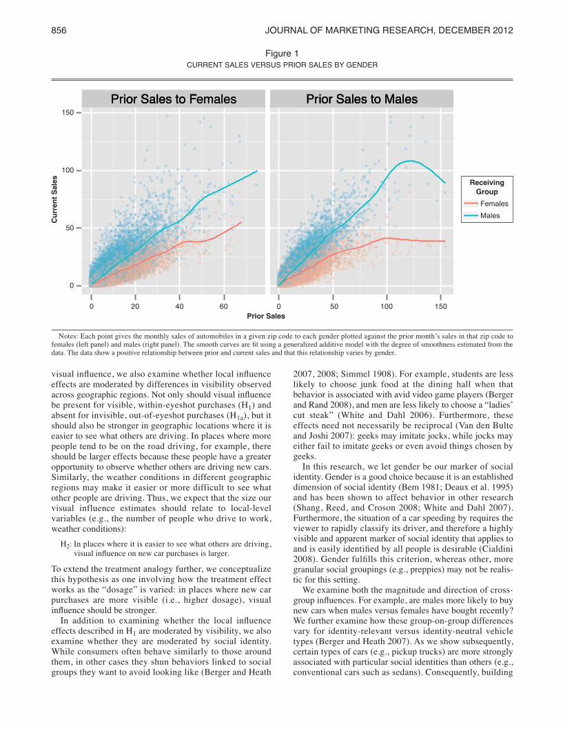
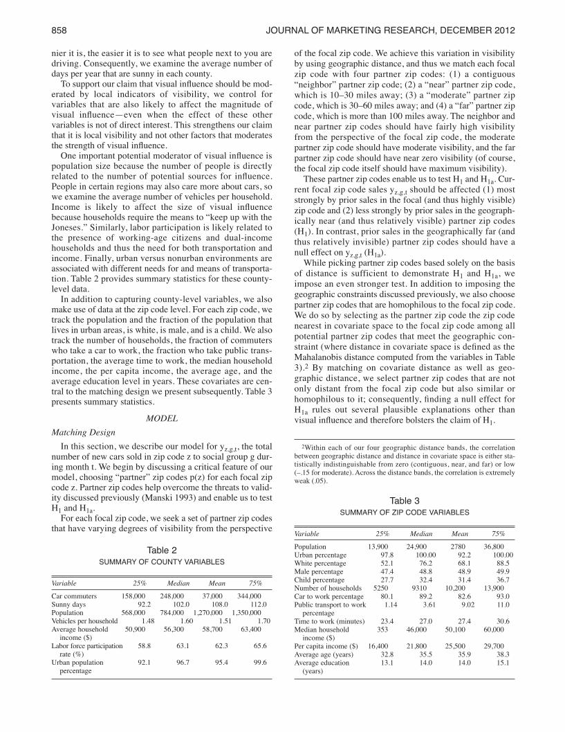
As an initial exploration of this phenomenon, considerFigure 1, which plots the monthly sales of automobiles in agiven zip code to each gender against the prior month’ssales in that zip code to females (left panel) and males (rightpanel). There are several noteworthy features. First, there isa positive relationship between prior and current sales (i.e.,the smooth curves generally slope upward), suggesting apotential for visual influence. Second, this relationshipappears to vary by the “sending” (i.e., compare gendersacross panels) and “receiving” (i.e., compare genders withinpanels) groups. That is, the four plotted curves are not iden-tical. Third, the relationship appears subject to saturationeffects (i.e., the curves tend to flatten out as prior salesincrease)—a phenomenon well-studied in marketing and inparticular in advertising (Dubé, Hitsch, and Manchanda2005; Johansson 1973; Laurent, Kapferer, and Roussel1995).
Before examining these issues, we first lay out ourhypotheses beginning with the principal one:
H1: Consumers purchase more new cars when they have seenothers around them do so recently.
When people see others around them driving new cars, theyshould be more likely to purchase new cars themselves.Thus, recent prior purchases that are local, and thereforevisible, should have an impact on current purchases. Thatsaid, while people often see what their neighbors or otherpeople who live nearby are driving, they less frequently seethe cars driven by people who live farther away. Becausethey cannot see these “out of eyeshot” cars, they should notbe affected by them:
H1a: Consumers do not purchase more new cars when those outof eyeshot have done so recently.
While H1a can be viewed as an additional test of visibility(i.e., one cannot be influenced by something one cannotsee), it can also be viewed as a robustness check on H1;thus, we denote it “auxiliary” (H1a). If, by analogy to theexperimentation literature, H1 yields the hypothesized posi-tive “treatment” effect of visible prior purchases, H1a yieldsthe hypothesized null effect for the “control” or “placebo”condition of prior purchases that are far away and thusinvisible. Therefore, finding a null effect for H1a (i.e., noevidence of an effect for purchases that are out of eyeshot)is as important for our theory as finding a positive effect forH1 (i.e., evidence of an effect for purchases that are withineyeshot) because it provides additional evidence that anyobserved relationship between people’s purchases is drivenby visual influence.
As a further theoretical contribution and to more stronglydemonstrate that any observed relationships are driven by
H JMR 11 0223 Color Web Layout_JMR (2011 Specs) 11/9/12 11:16 AM Page 855
visual influence, we also examine whether local influenceeffects are moderated by differences in visibility observedacross geographic regions. Not only should visual influencebe present for visible, within-eyeshot purchases (H1) andabsent for invisible, out-of-eyeshot purchases (H1a), but itshould also be stronger in geographic locations where it iseasier to see what others are driving. In places where morepeople tend to be on the road driving, for example, thereshould be larger effects because these people have a greateropportunity to observe whether others are driving new cars.Similarly, the weather conditions in different geographicregions may make it easier or more difficult to see whatother people are driving. Thus, we expect that the size ourvisual influence estimates should relate to local-levelvariables (e.g., the number of people who drive to work,weather conditions):
H2: In places where it is easier to see what others are driving,visual influence on new car purchases is larger.
To extend the treatment analogy further, we conceptualizethis hypothesis as one involving how the treatment effectworks as the “dosage” is varied: in places where new carpurchases are more visible (i.e., higher dosage), visualinfluence should be stronger.
In addition to examining whether the local influenceeffects described in H1 are moderated by visibility, we alsoexamine whether they are moderated by social identity.While consumers often behave similarly to those aroundthem, in other cases they shun behaviors linked to socialgroups they want to avoid looking like (Berger and Heath
2007, 2008; Simmel 1908). For example, students are lesslikely to choose junk food at the dining hall when thatbehavior is associated with avid video game players (Bergerand Rand 2008), and men are less likely to choose a “ladies’cut steak” (White and Dahl 2006). Furthermore, theseeffects need not necessarily be reciprocal (Van den Bulteand Joshi 2007): geeks may imitate jocks, while jocks mayeither fail to imitate geeks or even avoid things chosen bygeeks.
In this research, we let gender be our marker of socialidentity. Gender is a good choice because it is an establisheddimension of social identity (Bem 1981; Deaux et al. 1995)and has been shown to affect behavior in other research(Shang, Reed, and Croson 2008; White and Dahl 2007).Furthermore, the situation of a car speeding by requires theviewer to rapidly classify its driver, and therefore a highlyvisible and apparent marker of social identity that applies toand is easily identified by all people is desirable (Cialdini2008). Gender fulfills this criterion, whereas other, moregranular social groupings (e.g., preppies) may not be realis-tic for this setting.
We examine both the magnitude and direction of cross-group influences. For example, are males more likely to buynew cars when males versus females have bought recently?We further examine how these group-on-group differencesvary for identity-relevant versus identity-neutral vehicletypes (Berger and Heath 2007). As we show subsequently,certain types of cars (e.g., pickup trucks) are more stronglyassociated with particular social identities than others (e.g.,conventional cars such as sedans). Consequently, building
856 JOURNAL OF MARKETING RESEARCH, DECEMBER 2012
Figure 1CURRENT SALES VERSUS PRIOR SALES BY GENDER
Prior Sales to Females Prior Sales to Males
ior Sales to FPr
emalesior Sales to F ior Sales to MalesPr
ior Sales to Males
150
100
50
0
Curre
nt Sales
20 40 60 0 50 100 1500
Notes: Each point gives the monthly sales of automobiles in a given zip code to each gender plotted against the prior month’s sales in that zip code tofemales (left panel) and males (right panel). The smooth curves are fit using a generalized additive model with the degree of smoothness estimated from thedata. The data show a positive relationship between prior and current sales and that this relationship varies by gender.
ReceivingGroup
FemalesMales
Prior Sales
H JMR 11 0223 Color Web Layout_JMR (2011 Specs) 11/9/12 11:20 AM Page 856
Visual Influence and Social Groups 857
on prior work demonstrating that people are more likely toavoid products associated with other social groups in iden-tity-relevant domains, positive cross-gender influenceeffects should be weaker in these more identity-relevant carcategories. More specifically, we hypothesize variation ininfluence effects by social group:
H3: Visual influence varies by sending/receiving groups. In par-ticular, the (fe)male sending group has a greater effect for(fe)male-oriented cars.
Comparing these relative effects both deepens our under-standing of visual influence and has important managerialimplications for targeting effects (Joshi, Reibstein, andZhang 2009).
We also test the functional form of visual effects. First,social effects are typically assumed to be linear andabsolute. However, Figure 1 suggests that saturation effects,commonly observed in other areas of marketing, may existfor visual influence. Consequently, we test a logistic specifi-cation in addition to a linear one. Second, because each geo-graphic region has a different volume of sales, we also testwhether the effects should be relative (i.e., whether absoluteprior sales should be used as the covariate or whether atransformation that accounts for the size relative to the vol-ume of new cars sold in that locale should be used). Finally,we also perform various robustness tests of our model,including a theoretically motivated one pertaining to theprice tier of the vehicle.
DATAPower Information Network Data
Our data on automobile purchases come from the J.D.Power and Associates Power Information Network (PIN).The PIN division was founded in 1993 with the objective ofcollecting car sales transaction data from a large sample ofdealerships representative of the U.S. market; currently,approximately one-third of U.S. dealers are enrolled in thenetwork. Each night, these dealers transmit their daily trans-actions to J.D. Power and Associates, which then makes thedata available to academic researchers (for more elaboratedescriptions of this network, see Bucklin, Siddarth, andSilva-Risso 2008; Busse, Simester, and Zettelmeyer 2010;Dasgupta, Siddarth, and Silva-Risso 2007; Scott-Morton,Zettelmeyer, and Silva-Risso 2001, 2003; Silva-Risso andIonova 2008; Srinivasan et al. 2004).
Our particular data set contains the number of automo-biles sold to each gender in 905 U.S. zip codes in eachmonth from January 1999 through March 2008.1 All 905 zipcodes are contained within C = 40 randomly sampled largeU.S. counties, and up to 25 zip codes were randomly sam-pled from each county (we have 905 < 40 ¥ 25 = 1000 zipcodes because some counties have fewer than 25 zip codes).
Note that our zip codes are those of the purchasers asopposed to the dealers.
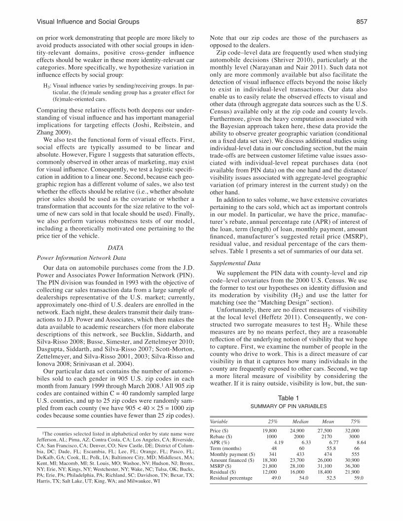
Zip code–level data are frequently used when studyingautomobile decisions (Shriver 2010), particularly at themonthly level (Narayanan and Nair 2011). Such data notonly are more commonly available but also facilitate thedetection of visual influence effects beyond the noise likelyto exist in individual-level transactions. Our data alsoenable us to easily relate the observed effects to visual andother data (through aggregate data sources such as the U.S.Census) available only at the zip code and county levels.Furthermore, given the heavy computation associated withthe Bayesian approach taken here, these data provide theability to observe greater geographic variation (conditionalon a fixed data set size). We discuss additional studies usingindividual-level data in our concluding section, but the maintrade-offs are between customer lifetime value issues asso-ciated with individual-level repeat purchases data (notavailable from PIN data) on the one hand and the distance/visibility issues associated with aggregate-level geographicvariation (of primary interest in the current study) on theother hand.
In addition to sales volume, we have extensive covariatespertaining to the cars sold, which act as important controlsin our model. In particular, we have the price, manufac-turer’s rebate, annual percentage rate (APR) of interest ofthe loan, term (length) of loan, monthly payment, amountfinanced, manufacturer’s suggested retail price (MSRP),residual value, and residual percentage of the cars them-selves. Table 1 presents a set of summaries of our data set.Supplemental Data
We supplement the PIN data with county-level and zipcode–level covariates from the 2000 U.S. Census. We usethe former to test our hypotheses on identity diffusion andits moderation by visibility (H2) and use the latter formatching (see the “Matching Design” section).
Unfortunately, there are no direct measures of visibilityat the local level (Heffetz 2011). Consequently, we con-structed two surrogate measures to test H2. While thesemeasures are by no means perfect, they are a reasonablereflection of the underlying notion of visibility that we hopeto capture. First, we examine the number of people in thecounty who drive to work. This is a direct measure of carvisibility in that it captures how many individuals in thecounty are frequently exposed to other cars. Second, we tapa more literal measure of visibility by considering theweather. If it is rainy outside, visibility is low, but, the sun-
1The counties selected listed in alphabetical order by state name wereJefferson, AL; Pima, AZ; Contra Costa, CA; Los Angeles, CA; Riverside,CA; San Francisco, CA; Denver, CO; New Castle, DE; District of Colum-bia, DC; Dade, FL; Escambia, FL; Lee, FL; Orange, FL; Pasco, FL;DeKalb, GA; Cook, IL; Polk, IA; Baltimore City, MD; Middlesex, MA;Kent, MI; Macomb, MI; St. Louis, MO; Washoe, NV; Hudson, NJ; Bronx,NY; Erie, NY; Kings, NY; Westchester, NY; Wake, NC; Tulsa, OK; Bucks,PA; Erie, PA; Philadelphia, PA; Richland, SC; Davidson, TN; Bexar, TX;Harris, TX; Salt Lake, UT; King, WA; and Milwaukee, WI
Table 1SUMMARY OF PIN VARIABLES
Variable 25% Median Mean 75%Price ($) 19,800 24,900 27,500 32,000Rebate ($) 1000 2000 2170 3000APR (%) 4.19 6.33 6.77 8.64Term (months) 48 60 55.8 66Monthly payment ($) 341 433 474 555Amount financed ($) 18,300 23,700 26,000 30,900MSRP ($) 21,800 28,100 31,100 36,300Residual ($) 12,000 16,000 18,400 21,900Residual percentage 49.0 54.0 52.5 59.0
H JMR 11 0223 Color Web Layout_JMR (2011 Specs) 11/9/12 11:20 AM Page 857
nier it is, the easier it is to see what people next to you aredriving. Consequently, we examine the average number ofdays per year that are sunny in each county.
To support our claim that visual influence should be mod-erated by local indicators of visibility, we control forvariables that are also likely to affect the magnitude ofvisual influence—even when the effect of these othervariables is not of direct interest. This strengthens our claimthat it is local visibility and not other factors that moderatesthe strength of visual influence.
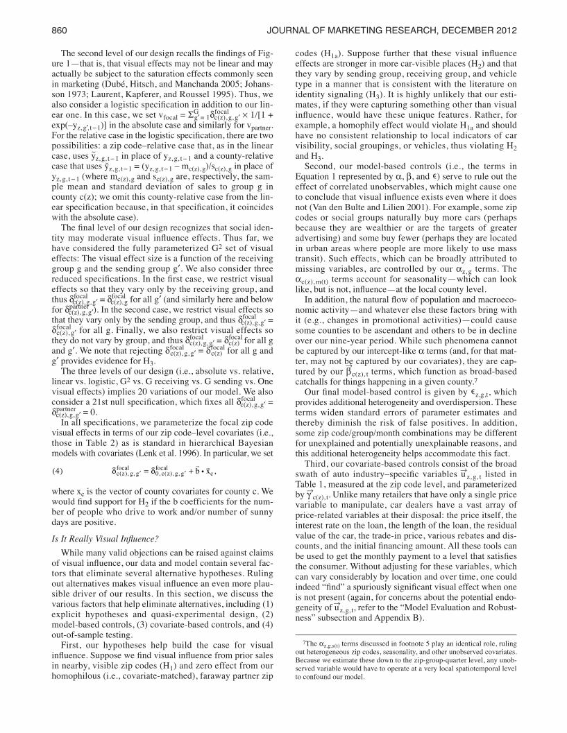
One important potential moderator of visual influence ispopulation size because the number of people is directlyrelated to the number of potential sources for influence.People in certain regions may also care more about cars, sowe examine the average number of vehicles per household.Income is likely to affect the size of visual influencebecause households require the means to “keep up with theJoneses.” Similarly, labor participation is likely related tothe presence of working-age citizens and dual-incomehouseholds and thus the need for both transportation andincome. Finally, urban versus nonurban environments areassociated with different needs for and means of transporta-tion. Table 2 provides summary statistics for these county-level data.
In addition to capturing county-level variables, we alsomake use of data at the zip code level. For each zip code, wetrack the population and the fraction of the population thatlives in urban areas, is white, is male, and is a child. We alsotrack the number of households, the fraction of commuterswho take a car to work, the fraction who take public trans-portation, the average time to work, the median householdincome, the per capita income, the average age, and theaverage education level in years. These covariates are cen-tral to the matching design we present subsequently. Table 3presents summary statistics.
MODELMatching Design
In this section, we describe our model for yz,g,t, the totalnumber of new cars sold in zip code z to social group g dur-ing month t. We begin by discussing a critical feature of ourmodel, choosing “partner” zip codes p(z) for each focal zipcode z. Partner zip codes help overcome the threats to valid-ity discussed previously (Manski 1993) and enable us to testH1 and H1a.
For each focal zip code, we seek a set of partner zip codesthat have varying degrees of visibility from the perspective
of the focal zip code. We achieve this variation in visibilityby using geographic distance, and thus we match each focalzip code with four partner zip codes: (1) a contiguous“neighbor” partner zip code; (2) a “near” partner zip code,which is 10–30 miles away; (3) a “moderate” partner zipcode, which is 30–60 miles away; and (4) a “far” partner zipcode, which is more than 100 miles away. The neighbor andnear partner zip codes should have fairly high visibilityfrom the perspective of the focal zip code, the moderatepartner zip code should have moderate visibility, and the farpartner zip code should have near zero visibility (of course,the focal zip code itself should have maximum visibility).
These partner zip codes enable us to test H1 and H1a. Cur-rent focal zip code sales yz,g,t should be affected (1) moststrongly by prior sales in the focal (and thus highly visible)zip code and (2) less strongly by prior sales in the geograph-ically near (and thus relatively visible) partner zip codes(H1). In contrast, prior sales in the geographically far (andthus relatively invisible) partner zip codes should have anull effect on yz,g,t (H1a).
While picking partner zip codes based solely on the basisof distance is sufficient to demonstrate H1 and H1a, weimpose an even stronger test. In addition to imposing thegeographic constraints discussed previously, we also choosepartner zip codes that are homophilous to the focal zip code.We do so by selecting as the partner zip code the zip codenearest in covariate space to the focal zip code among allpotential partner zip codes that meet the geographic con-straint (where distance in covariate space is defined as theMahalanobis distance computed from the variables in Table3).2 By matching on covariate distance as well as geo-graphic distance, we select partner zip codes that are notonly distant from the focal zip code but also similar orhomophilous to it; consequently, finding a null effect forH1a rules out several plausible explanations other thanvisual influence and therefore bolsters the claim of H1.
858 JOURNAL OF MARKETING RESEARCH, DECEMBER 2012
a
Table 2SUMMARY OF COUNTY VARIABLES
Variable 25% Median Mean 75%Car commuters 158,000 248,000 37,000 344,000Sunny days 92.2 102.0 108.0 112.0Population 568,000 784,000 1,270,000 1,350,000Vehicles per household 1.48 1.60 1.51 1.70Average household 50,900 56,300 58,700 63,400
income ($)Labor force participation 58.8 63.1 62.3 65.6
rate (%)Urban population 92.1 96.7 95.4 99.6
percentage
Table 3SUMMARY OF ZIP CODE VARIABLES
Variable 25% Median Mean 75%Population 13,900 24,900 2780 36,800Urban percentage 97.8 100.00 92.2 100.00White percentage 52.1 76.2 68.1 88.5Male percentage 47.4 48.8 48.9 49.9Child percentage 27.7 32.4 31.4 36.7Number of households 5250 9310 10,200 13,900Car to work percentage 80.1 89.2 82.6 93.0Public transport to work 1.14 3.61 9.02 11.0
percentageTime to work (minutes) 23.4 27.0 27.4 30.6Median household 353 46,000 50,100 60,000
income ($)Per capita income ($) 16,400 21,800 25,500 29,700Average age (years) 32.8 35.5 35.9 38.3Average education 13.1 14.0 14.0 15.1
(years)
2Within each of our four geographic distance bands, the correlationbetween geographic distance and distance in covariate space is either sta-tistically indistinguishable from zero (contiguous, near, and far) or low(–.15 for moderate). Across the distance bands, the correlation is extremelyweak (.05).
H JMR 11 0223 Color Web Layout_JMR (2011 Specs) 11/9/12 11:20 AM Page 858
Visual Influence and Social Groups 859
We note that while matching on all possible covariateswould be the strongest test of all, matching on any covari-ates whatsoever provides a stronger test than matching onnone (i.e., other than distance). Furthermore, the covariateswe do match on are broad and include population, urbaniza-tion, race, household composition, age, commuting patterns,income, and education variables.Model Specification
Our principal specification for the count nature of the carpurchase volumes yz,g,t uses a heterogeneous Poisson3probability model, letting yz,g,t ~ Poisson(λz,g,t). The specifi-cation for λz,g,t is the heart of our model, and to test ourhypotheses, we try alternative specifications (detailed nextin the “Visual Effects Specifications” subsection), whichallow us to formally decide between models with and with-out various forms of visual influence effects. We begin bydiscussing our principal model for λz,g,t, which is given by
We step through this equation line by line, focusing most ofour discussion on the last line, which contains the terms thatare most central to our hypotheses.4
In the first line, the heterogeneous zip-group interceptparameters αz, g allow each social group in each zip code tobuy more or fewer cars per month than the overall average.The αc(z), m(t) parameters in the second line provide eachcounty with its own pattern of seasonality at the monthlylevel (c(z) is the county in which zip code z is located, andm(t) refers to the calendar month of time t). Next, there is acubic time trend parameterized by bÆc(z),g = (bc(z),g,1, bc(z),g,2,bc(z), g, 3), which allows for long, secular trends in eachcounty and captures the effects of missing covariates thatvary with time.5 Overdispersion is represented by z, g, t inthe fourth line and serves to dampen the effect of covariatesby widening the standard errors when the data require it. Incombination, the zip-group intercepts, seasonality, trends,
'
λ =
α
+ α
+ β + β + β
+
+ γ ×
+ +
(1) log( )
Zip Code-Group InterceptsCounty-Month Effects
t t t Time TrendsError / Overdispersion
u Car Covariates
v v Focal and PartnerVisual Effects
z,g,t
z,g
c(z),m(t)
c(z),g,1 c(z),g,22
c(z),g,33
z,g,t
c(z),g z,g, t
focal partner
σ (2) ~ N(0, ).z, g, t2
heterogeneity, and overdispersion of the first four lines alsohelp mitigate the potential effects of missing covariates(Van den Bulte and Lilien 2001).
The fifth line takes account of various variables pertain-ing to the local car market. In particular, the automobilecovariate vector uÆz, g, t contains the level of each of thevariables listed in Table 1 averaged across the yz,g,t automo-biles sold to group g in zip code z during month t. (We rec-ognize the potential endogeneity of uÆz,g, t; for further discus-sion, see the “Model Evaluation and Robustness” sectionand Appendix B.) The parameters gÆc(z), g allow each groupin each county to react differently to these automobilecovariates uÆz, g, t. This line of the equation thus adjusts formacro-level variations in salient automobile industry–specific variables (e.g., prices, interest rates) that are not ofprimary interest in this research.Visual Effect Specifications
The sixth and final line of Equation 1 is the one of pri-mary interest, and we consider a model design with threelevels, resulting in a total of 20 specifications (plus a 21st“null” specification). Before introducing the design, we pro-vide an initial “base” specification, which is given by
This specification posits that current sales in the focal zipcode are affected in an absolute sense by the previousmonth’s sales in the focal zip code, that the effect is linear,and that there are G2 effects dc(z), g, g¢ (i.e., the visual effectsize depends on the receiving group g and the sending groupg¢).6 We would find evidence for H1 when dfocal
c(z), g, g¢ ≥ 0.For this and all other specifications, vpartner has an identi-
cal form to vfocal but with coefficients dpartnerc(z), g, g¢ in place of
dfocalc(z), g, g¢ and prior sales in the partner zip code yp(z), g¢, t − 1 in
place of prior sales in the focal zip code yz, g¢, t − 1. Thus, thebase specification for vpartner is given by vpartner = SG
g¢ = 1dpartner
c(z), g, g¢yp(z), g¢, t − 1. We would find support for H1a when dpartner
c(z), g, g¢ is statistically no different from zero for far partnerzip codes.
The first level of our design recognizes that visual effectsmay operate on a relative level rather than an absolute level(as in Equation 3). For example, one additional new car onthe road may mean something very different in a place wheremany versus few new cars are sold each month. While our dparameters have a subscript c(z) and thus allow for varia-tion in the size of visual effects across counties, there is anadditional way to allow for variation: rather than usingabsolute lag sales in our model, we use a relative version,which is standardized at the zip code level. Namely, we setvfocal = SG
g¢= 1dfocalc(z), g, g¢y~z, g¢, t − 1, where y~z, g¢, t − 1 = (yz, g¢, t − 1 –
mz, g)/sz, g and mz, g and sz, g are, respectively, the samplemean and standard deviation of sales to group g in zip codez. Again, we use the same relative specification for vpartner.
∑= δ ′′ =
′ −(3) v y .focal c(z), g, gfocal
g 1
Gz, g , t 1
3While a Poisson model is appropriate for data supported on the nonneg-ative integers (i.e., count data) such as ours, we also confirmed that ourresults did not change if we instead employed a Gaussian likelihood(though we modeled ÷yz, g, t + 1/4 rather than yz,g,t in the Gaussian case;Brown, Cai, and DasGupta 2006; DasGupta 2008).
4We discuss and lay out the priors in detail in Appendix A. Simply put,we use the standard ones for Bayesian hierarchical models.
5Analyses showed that cubics were sufficiently flexible; as a robustnesscheck, we replaced az, g + ac(z), m(t) + bc(z), g, 1t + bc(z), g, 2t2 + bc(z), g, 3t3 byzip code/group/time-specific parameters az,g,s(t), where we set s(t) succes-sively at the annual, semiannual, and quarterly levels. All results remainedqualitatively similar.
6We note that our hypotheses are about “recent” sales and not the previ-ous month’s sales in particular. Although we operationalize recent saleshere as the previous month’s sales, we tested the robustness of this defini-tion by using the previous quarter’s sales as well as the previous sixmonths’ sales in place of the previous month’s sales, and our resultsremained qualitatively similar.
H JMR 11 0223 Color Web Layout_JMR (2011 Specs) 11/9/12 11:20 AM Page 859
The second level of our design recalls the findings of Fig-ure 1—that is, that visual effects may not be linear and mayactually be subject to the saturation effects commonly seenin marketing (Dubé, Hitsch, and Manchanda 2005; Johans-son 1973; Laurent, Kapferer, and Roussel 1995). Thus, wealso consider a logistic specification in addition to our lin-ear one. In this case, we set vfocal = SG
g¢= 1dfocalc(z), g, g¢ ¥ 1/[1 +
exp(–yz, g¢, t−1)] in the absolute case and similarly for vpartner.For the relative case in the logistic specification, there are twopossibilities: a zip code–relative case that, as in the linearcase, uses y~z, g, t − 1 in place of yz, g, t − 1 and a county-relativecase that uses yz, g, t−1 = (yz, g, t−1 – mc(z), g)/sc(z), g in place ofyz, g, t − 1 (where mc(z), g and sc(z), g are, respectively, the sam-ple mean and standard deviation of sales to group g incounty c(z); we omit this county-relative case from the lin-ear specification because, in that specification, it coincideswith the absolute case).
The final level of our design recognizes that social iden-tity may moderate visual influence effects. Thus far, wehave considered the fully parameterized G2 set of visualeffects: The visual effect size is a function of the receivinggroup g and the sending group g¢. We also consider threereduced specifications. In the first case, we restrict visualeffects so that they vary only by the receiving group, andthus dfocal
c(z), g, g¢ = dfocalc(z), g for all g¢ (and similarly here and below
for dpartnerc(z), g, g¢). In the second case, we restrict visual effects so
that they vary only by the sending group, and thus dfocalc(z), g, g¢ =
dfocalc(z), g¢ for all g. Finally, we also restrict visual effects so
they do not vary by group, and thus dfocalc(z), g, g¢ = dfocal
c(z) for all gand g¢. We note that rejecting dfocal
c(z), g, g¢ = dfocalc(z) for all g and
g¢ provides evidence for H3.The three levels of our design (i.e., absolute vs. relative,
linear vs. logistic, G2 vs. G receiving vs. G sending vs. Onevisual effects) implies 20 variations of our model. We alsoconsider a 21st null specification, which fixes all dfocal
c(z), g, g¢ =dpartner
c(z), g, g¢ = 0.In all specifications, we parameterize the focal zip code
visual effects in terms of our zip code–level covariates (i.e.,those in Table 2) as is standard in hierarchical Bayesianmodels with covariates (Lenk et al. 1996). In particular, we set
where xc is the vector of county covariates for county c. Wewould find support for H2 if the b coefficients for the num-ber of people who drive to work and/or number of sunnydays are positive.Is It Really Visual Influence?
While many valid objections can be raised against claimsof visual influence, our data and model contain several fac-tors that eliminate several alternative hypotheses. Rulingout alternatives makes visual influence an even more plau-sible driver of our results. In this section, we discuss thevarious factors that help eliminate alternatives, including (1)explicit hypotheses and quasi-experimental design, (2)model-based controls, (3) covariate-based controls, and (4)out-of-sample testing.
First, our hypotheses help build the case for visualinfluence. Suppose we find visual influence from prior salesin nearby, visible zip codes (H1) and zero effect from ourhomophilous (i.e., covariate-matched), faraway partner zip
(4) b x ,c(z), g, g
focal0, c(z), g, gfocal
cδ = δ +′ ′
codes (H1a). Suppose further that these visual influenceeffects are stronger in more car-visible places (H2) and thatthey vary by sending group, receiving group, and vehicletype in a manner that is consistent with the literature onidentity signaling (H3). It is highly unlikely that our esti-mates, if they were capturing something other than visualinfluence, would have these unique features. Rather, forexample, a homophily effect would violate H1a and shouldhave no consistent relationship to local indicators of carvisibility, social groupings, or vehicles, thus violating H2and H3.
Second, our model-based controls (i.e., the terms inEquation 1 represented by a, b, and ) serve to rule out theeffect of correlated unobservables, which might cause oneto conclude that visual influence exists even where it doesnot (Van den Bulte and Lilien 2001). For example, some zipcodes or social groups naturally buy more cars (perhapsbecause they are wealthier or are the targets of greateradvertising) and some buy fewer (perhaps they are locatedin urban areas where people are more likely to use masstransit). Such effects, which can be broadly attributed tomissing variables, are controlled by our az, g terms. Theac(z), m(t) terms account for seasonality—which can looklike, but is not, influence—at the local county level.
In addition, the natural flow of population and macroeco-nomic activity—and whatever else these factors bring withit (e.g., changes in promotional activities)—could causesome counties to be ascendant and others to be in declineover our nine-year period. While such phenomena cannotbe captured by our intercept-like a terms (and, for that mat-ter, may not be captured by our covariates), they are cap-tured by our bÆc(z), t terms, which function as broad-basedcatchalls for things happening in a given county.7
Our final model-based control is given by z,g,t, whichprovides additional heterogeneity and overdispersion. Theseterms widen standard errors of parameter estimates andthereby diminish the risk of false positives. In addition,some zip code/group/month combinations may be differentfor unexplained and potentially unexplainable reasons, andthis additional heterogeneity helps accommodate this fact.
Third, our covariate-based controls consist of the broadswath of auto industry–specific variables uÆz, g, t listed inTable 1, measured at the zip code level, and parameterizedby gÆc(z), t. Unlike many retailers that have only a single pricevariable to manipulate, car dealers have a vast array ofprice-related variables at their disposal: the price itself, theinterest rate on the loan, the length of the loan, the residualvalue of the car, the trade-in price, various rebates and dis-counts, and the initial financing amount. All these tools canbe used to get the monthly payment to a level that satisfiesthe consumer. Without adjusting for these variables, whichcan vary considerably by location and over time, one couldindeed “find” a spuriously significant visual effect when oneis not present (again, for concerns about the potential endo-geneity of uÆz, g, t, refer to the “Model Evaluation and Robust-ness” subsection and Appendix B).
'
'
860 JOURNAL OF MARKETING RESEARCH, DECEMBER 2012
7The az,g,s(t) terms discussed in footnote 5 play an identical role, rulingout heterogeneous zip codes, seasonality, and other unobserved covariates.Because we estimate these down to the zip-group-quarter level, any unob-served variable would have to operate at a very local spatiotemporal levelto confound our model.
H JMR 11 0223 Color Web Layout_JMR (2011 Specs) 11/9/12 11:20 AM Page 860
Visual Influence and Social Groups 861
Although there may be several relevant variables (e.g.,local inventory levels) for which we cannot explicitly con-trol, such variables are fortunately very likely to be highlycorrelated with variables we do control for. For example, ifinventories are high, dealers are likely to offer price incen-tives, thus leading to a correlation between inventory levelsand price. Such correlations allow the variables we have toat least partially adjust for these omitted ones. Although thisis often undesirable in research (in which, e.g., a researcheris interested in the coefficient on price but is lacking inven-tory information), in our setting, these correlated variablesserve as controls (i.e., we are not interested in their coeffi-cient estimates), and therefore there is much less concern.
Fourth and finally, we use out-of-sample and robustnesstests to evaluate our model. If our observed effects are spu-rious, out-of-sample predictions are likely to degrade sub-stantially. Furthermore, as detailed in “Model Evaluationand Robustness,” we provide several additional tests todemonstrate the strength of our model and the robustness ofits predictions.
RESULTSModel Specification Selection
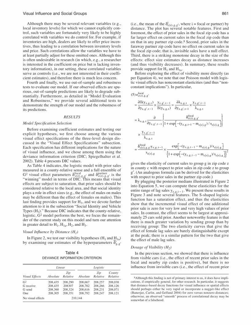
Before examining coefficient estimates and testing ourexplicit hypotheses, we first choose among the variousvisual effect specifications of the three-level design dis-cussed in the “Visual Effect Specifications” subsection.Each specification has different implications for the natureof visual influence, and we chose among them using thedeviance information criterion (DIC; Spiegelhalter et al.2002). Table 4 presents DIC values.
As Table 4 indicates, the logistic model with prior salesmeasured in a county-relative sense and a full ensemble ofG2 visual effect parameters dfocal
c(z), g, g¢ and dpartnerc(z), g, g¢ is the
“winning” model in terms of DIC. This means that visualeffects are subject to saturation, that prior sales should beconsidered relative to the local area, and that social identityplays a role in effect sizes (e.g., the effect of males on malesmay be different than the effect of females on males). Thislast finding provides support for H3, and we devote furtherattention to it in the subsection “Social Identity and VehicleTypes (H3).” Because DIC indicates that the county-relative,logistic, G2 model performs the best, we focus the remain-der of the current study on this model and turn our attentionin greater detail to H1, H1a, H2, and H3.Visual Influence by Distance (H1)
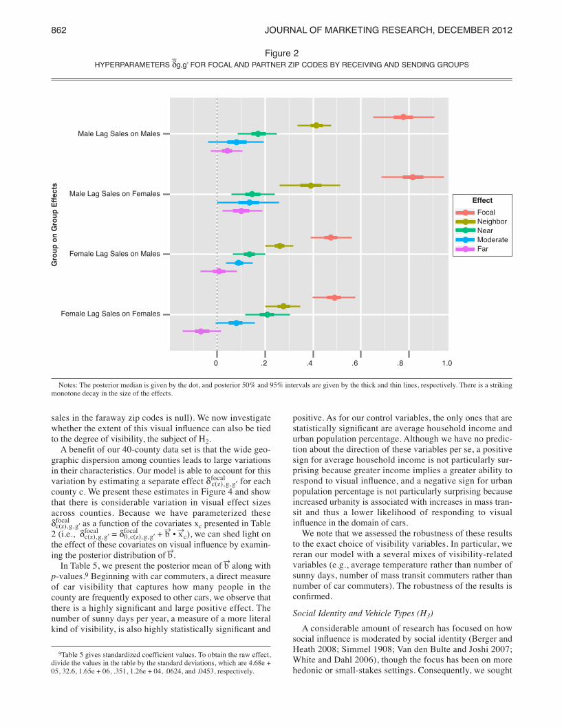
In Figure 2, we test our visibility hypotheses (H1 and H1a)by examining our estimates of the hyperparameters di
g, g¢
(i.e., the mean of the dic(z), g, g¢, where i = focal or partner) by
distance. The plot has several notable features. First andforemost, the effect of prior sales in the focal zip code has afar larger effect on current sales in the focal zip code thanon that in any partner zip code.8 Second, prior sales in thefaraway partner zip code have no effect on current sales inthe focal zip code; that is, invisible sales have a null effect.Third, there is a striking monotone decay in the size of theeffects: effect size estimates decay as distance increases(and thus visibility decreases). In summary, these resultsprovide support for H1 and H1a.
Before exploring the effect of visibility more directly (asper Equation 4), we note that our Poisson model with logis-tic visual effects has nonconstant elasticities (and thus “non-constant implications”). In particular,
gives the elasticity of current sales to group g in zip code zin county c with respect to prior sales in zip code z to groupg¢. (An analogous formula can be derived for the elasticitieswith respect to prior sales in the partner zip code.)
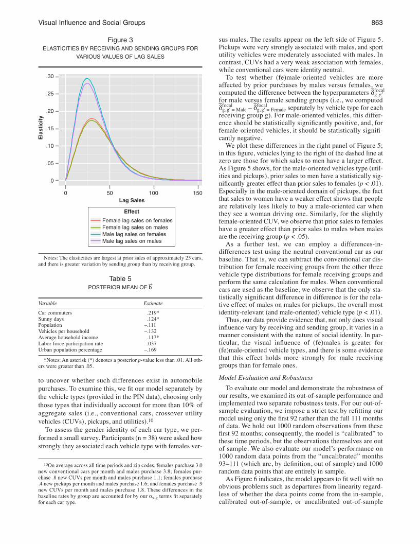
By plugging the posterior medians illustrated in Figure 2into Equation 5, we can compute these elasticities for theentire range of lag sales yz, g, t − 1. We present these results inFigure 3 and note several features. The S-shaped logisticfunction has a saturation effect, and thus the elasticitiesshow that the incremental visual effect of one additionalprior sale is zero for very low and very high values of priorsales. In contrast, the effect seems to be largest at approxi-mately 25 cars sold prior. Another noteworthy feature is thatthere is much greater variation by sending group than byreceiving group: The two elasticity curves that give theeffect of female lag sales are barely distinguishable exceptat the peak; there is a similar pattern for the two that givethe effect of male lag sales.Dosage of Visibility (H2)
In the previous section, we showed that there is influencefrom visible cars (i.e., the effect of recent prior sales in thefocal and nearby zip codes is positive), but there is noinfluence from invisible cars (i.e., the effect of recent prior
EE
(5) e(y )
yy
(y ) yy
y 1 exp (y m ) / s
y
ys
exp (y m )/s
1 exp (y m )/s
c(z), g, gfocal
z, g, tz, g , t 1
z, g , t 1z, g, t
z, g, tz, g , t 1
z, g , t 1z, g, t
z, g, tz, g , t 1
c(z), g, gfocal
z, g, t 1 c z , g c z , g
z, g , t 1z, g, t
c z , g, gfocal
z, g, t 1
c z , g
z, g, t 1 c z , g c z , g
z, g, t 1 c z , g c z , g2{ }
=∂∂
× =∂λ
∂×
λ
= λ∂
∂δ
+ − −
×λ
=δ
×− −
+ − −
( ) ( )
( )
( )
( ) ( )
( ) ( )
′
′ −
′ −
′ −
′ −
′ −
′
−
′ −
′ − −
−
Table 4DEVIANCE INFORMATION CRITERION
Linear LogisticZip Zip County
Visual Effects Absolute Relative Absolute Relative RelativeG2 208,435 208,290 208,667 208,257 208,038G receive 208,435 208307 208,782 208,266 208,126G send 208,360 208,324 208,616 208,231 208,071One 208,305 208,351 208,792 208,247 208,121No visual effects 210,144
8Although this finding is not of primary interest to us, it does have impli-cations, if empirically general, for other research. In particular, it suggeststhat distance-based decay functions for visual influence or spatial effectsshould perhaps either be very rapid or incorporate a nugget-like effect(Banerjee, Carlin, and Gelfand 2004) for zero versus nonzero distances;otherwise, an observed “smooth” process of correlational decay may besomewhat of a falsehood.
H JMR 11 0223 Color Web Layout_JMR (2011 Specs) 11/9/12 11:20 AM Page 861
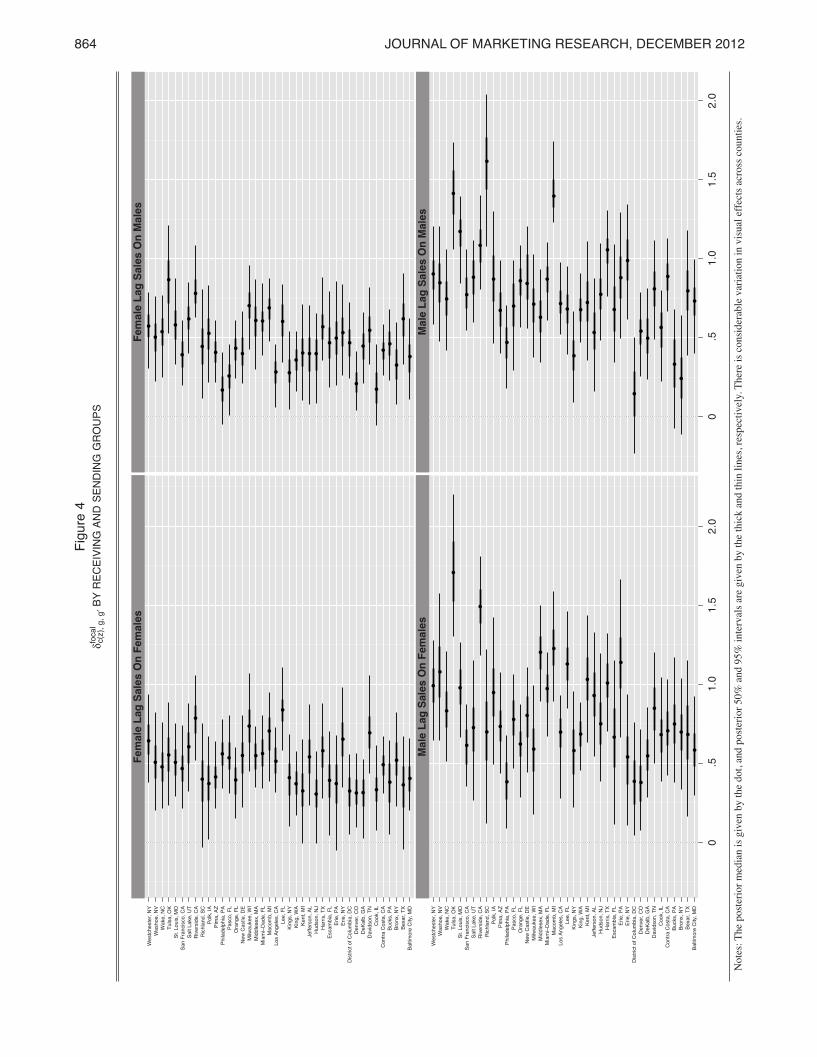
sales in the faraway zip codes is null). We now investigatewhether the extent of this visual influence can also be tiedto the degree of visibility, the subject of H2.
A benefit of our 40-county data set is that the wide geo-graphic dispersion among counties leads to large variationsin their characteristics. Our model is able to account for thisvariation by estimating a separate effect dfocal
c(z), g, g¢ for eachcounty c. We present these estimates in Figure 4 and showthat there is considerable variation in visual effect sizesacross counties. Because we have parameterized thesedfocal
c(z), g, g¢ as a function of the covariates xc presented in Table2 (i.e., dfocal
c(z), g, g¢ = dfocal0, c(z), g, g¢ + bÆ ∑ xÆc), we can shed light on
the effect of these covariates on visual influence by examin-ing the posterior distribution of bÆ.
In Table 5, we present the posterior mean of bÆ along withp-values.9 Beginning with car commuters, a direct measureof car visibility that captures how many people in thecounty are frequently exposed to other cars, we observe thatthere is a highly significant and large positive effect. Thenumber of sunny days per year, a measure of a more literalkind of visibility, is also highly statistically significant and
positive. As for our control variables, the only ones that arestatistically significant are average household income andurban population percentage. Although we have no predic-tion about the direction of these variables per se, a positivesign for average household income is not particularly sur-prising because greater income implies a greater ability torespond to visual influence, and a negative sign for urbanpopulation percentage is not particularly surprising becauseincreased urbanity is associated with increases in mass tran-sit and thus a lower likelihood of responding to visualinfluence in the domain of cars.
We note that we assessed the robustness of these resultsto the exact choice of visibility variables. In particular, wereran our model with a several mixes of visibility-relatedvariables (e.g., average temperature rather than number ofsunny days, number of mass transit commuters rather thannumber of car commuters). The robustness of the results isconfirmed.Social Identity and Vehicle Types (H3)
A considerable amount of research has focused on howsocial influence is moderated by social identity (Berger andHeath 2008; Simmel 1908; Van den Bulte and Joshi 2007;White and Dahl 2006), though the focus has been on morehedonic or small-stakes settings. Consequently, we sought
862 JOURNAL OF MARKETING RESEARCH, DECEMBER 2012
Figure 2HYPERPARAMETERS dg,g’ FOR FOCAL AND PARTNER ZIP CODES BY RECEIVING AND SENDING GROUPS
ll
ll
l
ll
ll
l
ll
ll
l
ll
ll
l
Male Lag Sales on Males
Male Lag Sales on Females
Female Lag Sales on Males
Female Lag Sales on Females
Grou
p on
Group
Effe
cts
.2 .4 .6 .80 1.0
Notes: The posterior median is given by the dot, and posterior 50% and 95% intervals are given by the thick and thin lines, respectively. There is a strikingmonotone decay in the size of the effects.
EffectFocalNeighborNearModerateFar
l
l
l
l
l
9Table 5 gives standardized coefficient values. To obtain the raw effect,divide the values in the table by the standard deviations, which are 4.68e +05, 32.6, 1.65e + 06, .351, 1.26e + 04, .0624, and .0453, respectively.
H JMR 11 0223 Color Web Layout_JMR (2011 Specs) 11/9/12 11:20 AM Page 862
Visual Influence and Social Groups 863
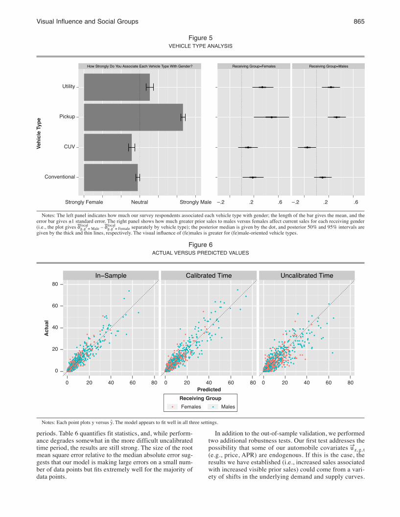
to uncover whether such differences exist in automobilepurchases. To examine this, we fit our model separately bythe vehicle types (provided in the PIN data), choosing onlythose types that individually account for more than 10% ofaggregate sales (i.e., conventional cars, crossover utilityvehicles (CUVs), pickups, and utilities).10
To assess the gender identity of each car type, we per-formed a small survey. Participants (n = 38) were asked howstrongly they associated each vehicle type with females ver-
sus males. The results appear on the left side of Figure 5.Pickups were very strongly associated with males, and sportutility vehicles were moderately associated with males. Incontrast, CUVs had a very weak association with females,while conventional cars were identity neutral.
To test whether (fe)male-oriented vehicles are moreaffected by prior purchases by males versus females, wecomputed the difference between the hyperparameters dfocal
g, g¢for male versus female sending groups (i.e., we computeddfocal
g, g¢ = Male – dfocalg, g¢ = Female separately by vehicle type for each
receiving group g). For male-oriented vehicles, this differ-ence should be statistically significantly positive, and, forfemale-oriented vehicles, it should be statistically signifi-cantly negative.
We plot these differences in the right panel of Figure 5;in this figure, vehicles lying to the right of the dashed line atzero are those for which sales to men have a larger effect.As Figure 5 shows, for the male-oriented vehicles type (util-ities and pickups), prior sales to men have a statistically sig-nificantly greater effect than prior sales to females (p < .01).Especially in the male-oriented domain of pickups, the factthat sales to women have a weaker effect shows that peopleare relatively less likely to buy a male-oriented car whenthey see a woman driving one. Similarly, for the slightlyfemale-oriented CUV, we observe that prior sales to femaleshave a greater effect than prior sales to males when malesare the receiving group (p < .05).
As a further test, we can employ a differences-in-differences test using the neutral conventional car as ourbaseline. That is, we can subtract the conventional car dis-tribution for female receiving groups from the other threevehicle type distributions for female receiving groups andperform the same calculation for males. When conventionalcars are used as the baseline, we observe that the only sta-tistically significant difference in difference is for the rela-tive effect of males on males for pickups, the overall mostidentity-relevant (and male-oriented) vehicle type (p < .01).
Thus, our data provide evidence that, not only does visualinfluence vary by receiving and sending group, it varies in amanner consistent with the nature of social identity. In par-ticular, the visual influence of (fe)males is greater for(fe)male-oriented vehicle types, and there is some evidencethat this effect holds more strongly for male receivinggroups than for female ones.Model Evaluation and Robustness
To evaluate our model and demonstrate the robustness ofour results, we examined its out-of-sample performance andimplemented two separate robustness tests. For our out-of-sample evaluation, we impose a strict test by refitting ourmodel using only the first 92 rather than the full 111 monthsof data. We hold out 1000 random observations from thesefirst 92 months; consequently, the model is “calibrated” tothese time periods, but the observations themselves are outof sample. We also evaluate our model’s performance on1000 random data points from the “uncalibrated” months93–111 (which are, by definition, out of sample) and 1000random data points that are entirely in sample.
As Figure 6 indicates, the model appears to fit well with noobvious problems such as departures from linearity regard-less of whether the data points come from the in-sample,calibrated out-of-sample, or uncalibrated out-of-sample
Figure 3ELASTICITIES BY RECEIVING AND SENDING GROUPS FOR
VARIOUS VALUES OF LAG SALES
.30
.25
.20
.15
.10
.05
0
Elastic
ity
Lag Sales500 100 150
Notes: The elasticities are largest at prior sales of approximately 25 cars,and there is greater variation by sending group than by receiving group.
EffectFemale lag sales on femalesFemale lag sales on malesMale lag sales on femalesMale lag sales on males
10On average across all time periods and zip codes, females purchase 3.0new conventional cars per month and males purchase 3.8; females pur-chase .8 new CUVs per month and males purchase 1.1; females purchase.4 new pickups per month and males purchase 1.6; and females purchase .9new CUVs per month and males purchase 1.8. These differences in thebaseline rates by group are accounted for by our az,g terms fit separatelyfor each car type.
Table 5POSTERIOR MEAN OF bÆ
Variable EstimateCar commuters .219*Sunny days .124*Population –.111Vehicles per household –.132Average household income .117*Labor force participation rate .037Urban population percentage –.169
*Notes: An asterisk (*) denotes a posterior p-value less than .01. All oth-ers were greater than .05.
H JMR 11 0223 Color Web Layout_JMR (2011 Specs) 11/9/12 11:20 AM Page 863
864 JOURNAL OF MARKETING RESEARCH, DECEMBER 2012
Figu
re 4
dfoca
lc(
z), g
, g¢BY
REC
EIVI
NG A
ND S
ENDI
NG G
ROUP
S
l
l
l
l
l
l
l
lll
l
l
l
l
l
l
l
l
l
l
l
l
ll
l
l
l
l
l
l
l
l
l
l
l
l
l
l
l
l
l
l
l
l
l
l
l
l
l
l
l
l
l
l
lll
l
l
l
l
l
ll
l
l
l
l
l
l
l
l
l
l
l
l
l
l
l
l
l
ll
l
l
l
l
l
ll
l
l
l
l
l
l
l
l
l
l
l
l
l
l
l
l
l
l
l
l
l
l
l
l
l
l
l
l
l
l
l
l
l
l
l
l
l
l
l
l
l
l
l
l
l
l
l
l
l
l
l
l
l
l
l
l
l
l
l
l
l
l
l
l
l
l
l
l
l
l
Fem
ale L
ag S
ales O
n Fe
male
sFe
male
Lag
Sale
s On
Male
s
Male
Lag
Sale
s On
Fem
ales
Male
Lag
Sale
s On
Male
s
Female La
g Sa
les On
Fem
ales
.50
1.0
1.5
2.0
.50
1.0
1.5
2.0
Notes
: The
poste
rior m
edian
is gi
ven b
y the
dot, a
nd po
sterio
r 50%
and 9
5% in
terva
ls are
give
n by t
he th
ick an
d thin
lines,
resp
ectiv
ely. T
here
is co
nside
rable
varia
tion i
n visu
al eff
ects
acros
s cou
nties.
Wes
tches
ter,
NYW
asho
e, N
VW
ake,
NC
Tulsa
, OK
St. L
ouis,
MO
San
Fran
cisco
, CA
Salt L
ake,
UT
Rive
rside
, CA
Rich
land,
SC
Polk,
IAPi
ma,
AZ
Phila
delph
ia, P
APa
sco,
FL
Oran
ge, F
LNe
w Ca
stle,
DE
Milw
auke
e, W
IM
iddles
ex, M
AM
iami−
Dade
, FL
Mac
omb,
MI
Los A
ngele
s, CA
Lee,
FL
King
s, NY
King
, WA
Kent
, MI
Jeffe
rson
, AL
Huds
on, N
JHa
rris,
TXEs
cam
bia, F
LEr
ie, P
AEr
ie, N
YDi
strict
of C
olum
bia, D
CDe
nver
, CO
DeKa
lb, G
ADa
vidso
n, T
NCo
ok, I
LCo
ntra
Cos
ta, C
ABu
cks,
PABr
onx,
NYBe
xar,
TXBa
ltimor
e Ci
ty, M
D
Female La
g Sa
les On
Males
Male La
g Sa
les On
Fem
ales
Male La
g Sa
les On
Males
H JMR 11 0223 Color Web Layout_JMR (2011 Specs) 11/9/12 11:20 AM Page 864
Visual Influence and Social Groups 865
periods. Table 6 quantifies fit statistics, and, while perform-ance degrades somewhat in the more difficult uncalibratedtime period, the results are still strong. The size of the rootmean square error relative to the median absolute error sug-gests that our model is making large errors on a small num-ber of data points but fits extremely well for the majority ofdata points.
In addition to the out-of-sample validation, we performedtwo additional robustness tests. Our first test addresses thepossibility that some of our automobile covariates uÆz, g, t(e.g., price, APR) are endogenous. If this is the case, theresults we have established (i.e., increased sales associatedwith increased visible prior sales) could come from a vari-ety of shifts in the underlying demand and supply curves.
Figure 5VEHICLE TYPE ANALYSIS
How Strongly Do You Associate Each Vehicle Type With Gender?
C
Receiving Group=Females Receiving Group=Males
l
l
l
l
l
l
l
lUtility
Pickup
CUV
Conventional
Vehicle Type
.2 .6Strongly Female Neutral Strongly Male –.2 .2 .6–.2
Notes: The left panel indicates how much our survey respondents associated each vehicle type with gender; the length of the bar gives the mean, and theerror bar gives ±1 standard error. The right panel shows how much greater prior sales to males versus females affect current sales for each receiving gender(i.e., the plot gives dfocal
g, g¢ = Male – dfocalg, g¢ = Female separately by vehicle type); the posterior median is given by the dot, and posterior 50% and 95% intervals are
given by the thick and thin lines, respectively. The visual influence of (fe)males is greater for (fe)male-oriented vehicle types.
Figure 6ACTUAL VERSUS PREDICTED VALUES
l
l
l
l
l
l
l
l
lll
l
ll
l
l
ll
l
ll
l
l
l
l
l
l
l
ll
ll
l
l
ll
ll
l
l
l
l
lll
ll
l
l
l
l
l
l
l
l
l
ll
l
l
l
l
l
lll
ll
l
l
l
l
l
l
l
l
ll
l
l
ll
l
l
l
l
l
lll
ll
l
ll
l
ll
l
l
ll
l
l
l
l
l
l
llll
l
ll
ll
lll
l
l
l
lll
l
l
l
l
ll
ll
ll
l
l
l
l
l
l
ll
l
l
l
l
l
l
ll
l
l
l
l
l
l
l
ll
l
l
l
ll
l
l
ll
l
ll
l
l
l
l
l
lll
l
l
l
l
ll
l
l
l
l
l
l
l
ll
l
l
l
l
l
l
l
l
l
ll
llll
l
l
ll
l
ll
l
l
l
l
l
l
lll
l
ll
l
l
l
l
ll
l
l
lll
l
l
l
l
l
l
l
l
l
l
l
l
l
l
ll
l
l
l
l
l
l
l
ll
l
l
l
l
l
l
l
l
l l
l
ll
ll
l
l
ll
l
l
l
l
ll
l
l
lll
l
ll
l
l
l
l
l
ll
l
l
l
lll
l
l
ll
l
l
ll
l
ll
l
l
l
l
l
l
l l
l
l
ll
l
l
l
ll l
l
l
l
l
l
l
l
l
l
l
l
l
l
ll
l
l
l
l l
l
l
l
l
lll
l
ll l
l
lll
l
l
l
l
l
ll
l
l
ll
l
ll
lll
ll
l
ll
l
l
l
l
l
ll
l
l
llll
l
ll
l
l
lll
l
l
ll
ll
l
llll
l
l
ll
l
l
l
l
ll
l
lll
l
ll
l ll
l
ll
lll
l
l
ll
l
l
ll
l
l
ll
ll
ll
ll
l
ll
lll
l
ll
l
ll
l
l
l
l
l
l
ll
ll
l
ll
l
l
l
l
ll
l
l
l
lll
lll
l
l
ll
l
ll
l
l
l
ll
ll
l
l
l
ll
l l
l
lllll
ll
l
l
l
l
ll
l
l
lll
l
llll
l
llll
ll
l
l
l
ll
ll
ll
ll
l
l
l
l
l
l
ll
l
l
l
l
l
l
l
l
l
l
l
l
l
ll
l
l
l
ll
lll
lll
l
l
l
l
l
l
ll
l
l
l
ll
l
l
ll
ll
l
l
l
l
l
l
l
l
l
l
lll
ll
l
l
l
ll
l
l
l
l
l
l
l
l
ll
l
ll
ll
ll
ll
l
lll
l
l
lllll
l
ll
l
l
l
l
ll
ll
l
ll
lll
l
l
ll
l
l
l
ll
ll
l
llll
l
l
l
ll
l
l
ll
l
l
l
l
l
l
l
l
l
l
ll
l
l
l
l
l
lll
l
l
l
l
l
ll
ll
ll
l
l
l
ll
l
ll
l
ll
l
l
l
l
l
l
l
l
l
ll
ll
l
l
l
l
ll
l
l
l
l
l
l
l
l
ll
l
l
l
l
l
l
l
l
l l
l
l
l
l
l
l
l
l
l
l
l
l
ll
l
l
l
l
l
l
l
l
ll
l
ll
l
l
lll
ll
l
l
l
l
l
l
l
l
l
ll
l
l
ll
l
l
ll
l
l
l
l
l
lll
l
l
l
l
l
l
ll
lll
l
l
lll
l
l
l
l
ll
ll
ll
l
lllll
l
l
ll
l
l
l
l
l
l
l
l
lll
l
l
l
l
l
l
l
l
l
ll
ll
l
l
l
ll
l
l
llll
ll ll
ll
l
l
l
l
ll
ll
l
lll
l
lll
l
l
l
l
l
l
l
ll
l
l
l
l
l
ll
ll
lll
l
l
l
l
ll
l
ll
ll
l
l
ll
ll
l
ll
l
l
l
ll
ll
l
l
l
l
l
l
l
l
l
l
l
ll
lll
l
l
ll
l
l
l
l
ll
l
l
l
l
ll
ll
l lll
l
l
l
l
l
l
l
l
l
l
l
l
ll
ll
ll
l
l
l
l
l
l
l
l
l
l
l
l
ll
l
l
l
l
lll
l
l
l
l
l
l
l
ll
l
l l
l
ll
l
l
l
l
l
l
l
l
l
l
l
l
l
l
l
llll
l
l
l
l
l
ll
ll
l
l
l
l
l
ll
ll
l
l
l
ll
l
l
l
ll
ll
l
l
l
l
ll
l
l
l
l
ll
l
l
l
l
ll
l
ll
l
l
l
l
l
l
l
lll
l
l
ll
l
ll
llllll
l
l
ll
l
l
l
l
l
l
l
l
l
ll
l
lll
l
l
l
l
l
l
l
l
ll
l
l
ll
l
l
l
ll
l
l
ll
l
ll
l
l
l
l
l
l
l
l
l
llll
l
ll
l
l
ll
ll
l
l
l
ll
ll
l
ll
l
l
ll
l
l
l
llll
l
ll l
l
l
ll
l
l
l
l
ll
l
ll
l
l
l
l
l
l
l
ll l
ll
l
l
l
l
l
l
l
l
ll
l
ll
l
l
ll
l
l
l
ll
l
l
l
l
l
l
l
l
l
llll
l
l
l
l
l
ll
lll
l
lll
ll
ll
l
l
lll
l
l
l
l
l
ll
l
ll
l
lll
ll
ll
l
l
l
l
ll
l
l
l
l
lll
l
l
l
l
l
l
l
l
l
l
l
ll
l
l
l
l
l
l
l
l
l
l
l
l
l
l
l
l
l l
l
l
l
ll
ll
l
l
ll
l
l
ll
ll l
l
l
l
l
l
lll
ll
l
ll
l
l
l
l
ll
l
l
lll
l
l
l
ll
l
l
l
l
l
ll
l
l
l
l
ll
l
l
l
ll
ll
l
l
l
l
ll
l
l
l
lll
l
ll
l
l
l
ll
l
l
l
l
lll
l
ll
lll l
l
l
l
l
l
l
l
ll
l
l
l
l
l
ll
l
l
l
l
l
l
l
l
l
l
ll
ll
l
l
l
l
l
lll
ll
l l
l
l
ll
l
l
l
l
l
l
l
l
l
l
ll
l
l
l
l
l
l
l
l
ll
ll
l
lll
ll
l
ll
l
l
l
l
l
l
l
l
l
l
l
l
l
l
l
l
l
l
l
l
l
l
l
ll
l l
l
l
l
ll
l
l
l
l
l
l
l
l
l
l
l
l
l
ll
l
l
ll
ll
l
ll
l
l
l
lll
l
l
l
l
l
l
lll
l
l
l
l
l
l
l
l
ll
l
l
l
l
l
l
l
l
l
ll
l
l
l
ll
l
ll
l
l
l
lll
l
ll
l
l
l
l
l
l
l
l
l
l
l
l
l
l ll
l
l
l
ll
l
ll
l
l
l
l
l
ll
l
l
l
l
l
l
l
lll
l
l
ll
l
l
l
l
l
l
l
l
l
ll
l
l
ll
ll
l
l
l
l
ll
ll
l
l
l
l
l
l lll
l
ll
ll
l
l
ll
lll
l
l
l
l
l
l
ll
ll
ll
l
l
l
l
l
l
l
l
ll
l
l
l
l
l
l
ll
l
ll
l
l
l
l
ll
l
l
llll
l
l
l
l
ll
l
ll
l
l
l
l
l
l
l
l
l
l
l
l
l
l
l
l
l
l
ll
l
ll
l
l
l
ll
l
l
lll
l
l
ll
ll
l
l
l
l
l
ll
l
l
l
ll
l
l
l
llllll
l
l
l
l
l
l
l
l
l
l
l
l
lll
l
l
lllll
l
l
l
l
l
ll
l
ll
l
l
ll
l
l
ll
l
l
l
l
l
l
l
l
l
l
l
l
l
l
l
ll
l
l
l
l l
ll
lll
ll
l
l
ll
l
l
ll
l
ll
l
l
l
l
l
l
l
ll
ll
l
l
ll
l
l
l
l
l
l
l
l
l
l
l
l
l
l
l
ll
l
l
l
l
l
ll
l
l
ll
l
l
ll
l
l
l
ll
l
ll
l
ll ll
l
ll
l
l
l
l
lll
l
l
l l
ll
l
l
l l
l
l
l
ll
l
l
l
ll
ll
l
l
l
l
l
l
l
ll
l
l
l
l
l
l
l
l
l
l
ll
l
ll l
l
l
ll
l
ll
l
l
l
l
ll
lll
ll
l
l
l
l
l
ll
l
l
l
ll
l
l
ll
l
l
ll
ll
l
l
l
lll
l
l
l
l
l
l
l
l
l
l
l
l
l
l
l
l
l
lll
l
l
lll
l
l
l
ll
l
l
l
l
l
l
ll
l
l
l
l
l
ll
l
l
l
lll
l
l
l
l
l
ll
l
l
ll
l
ll
lll
ll l
ll
l
l
l
l
l
l
lll
l
l
l
l
l
l
ll
l
l
l
l
ll
ll
l
l
l
l
l
l
l
l
ll
l
ll
l
l
l
l
l
l
ll
ll
l
l
l
l
l
l
ll
l
l
l
l
l
l
l
l
l l
l
l
lll
ll
l
l
l
l
l
l
lll
ll
l
l
l
ll
l
l
l
l
ll
l
l
lll
ll
l
l
l
l
l
lll
l
l
l
l
l
l
l
l
l
l
l
ll
l
l
ll
ll
ll
l
ll
l
l
l
ll
ll
l
l
ll
l
l
l
l
ll
l
l
l
l
l
l
l
l
ll
l
l
ll
ll
l lll
l
l
l
l
l
ll
l
l
l
l
ll
l
ll
l
lll
l
l
l
l
l
ll
l
l
lll
l
ll
ll
l
l
l
l
l
l
ll
l
l
l
l
l
ll
l
l
l
l
l
l
l
l
ll
l
l
l l
l
ll
l
ll
l
l
l
l
l
l
l
l
l
ll
lll
l
l
ll
ll
l
l
l
l
l
l
l
l
l
l
l
l
l l
l
l
l
l
l
l
l
l
l
l
l
l
ll
l
l
l
l
l
l
l
ll
l
l
l
l
l
lll
ll
ll
ll
l
l
l
l
l
l
ll
l
l
l
l
l
ll
ll
l
l
l
ll
ll ll
l
l
l
l
l
l
ll
l
l
l
ll
l
l
l
l
l
lll
l
l
l
ll
lll
l
ll
l
l
l
l
l
l
l
l
l
l
ll
l
l
l
l
l
l
ll
ll
l
l
l
l
ll
ll
l
l
l
l
l
l
l
l
ll
ll
l
ll
l
l
l
ll
l
l
ll
l
l
l
l
ll
l
l
ll
l
ll
l
l
l
l
l
ll
l
ll
l
l
l
l
l
l
l
ll
l
l
l
l
ll
ll
l
l
l
ll
l
l
l
l
l
l
l
l
l
l
l
l
l
l
l
l
ll
l
l
l
l
l
l
l
l
l
ll
l
ll
l
l
l
ll
l
ll
l
l
l
l
l
l
l
l
l
ll
l
ll
l
l
l
l
l
lll
l
l
l
l
l
l
l
l
l
l
l
l
l
ll
l
ll
l
l
l
l
lll
l
l
l
l
lll
l
l
lll
l
l
l
ll
l
ll
l
l
l
lll
l
l
ll
l
l
ll
ll
l
l
ll
l
lll
ll
ll
l
l
l
l
l
ll
ll
l
l
l
l
l
ll
ll
l
l
l
l
l
l
l
l
ll
l
l
l
ll
l
l
l
l
l
ll
ll
l
l
l
l
l
l
ll
ll
l
ll
ll
l
ll
l
l
l
l
l
l
l
l
ll
l
l
l
lll
ll
l
ll
ll ll
l
ll
l
l
l
l
ll
l
l
ll
l
l ll
l
l
l
l
l
ll
l
l
l
l
l
l
l
l
l
ll
l
l
l
ll
ll
l
l
l
l
l
llll
l
l
l
l
ll
l
l
l
ll
l
l
l
l
l
In−Sample Calibrated Time Uncalibrated Time
0
80
60
40
20
0
Actual
Predicted20 40 60 80 0 20 40 60 80 0 20 40 60 80 0
Notes: Each point plots y versus y. The model appears to fit well in all three settings.
Receiving GroupFemales Males
l
l
H JMR 11 0223 Color Web Layout_JMR (2011 Specs) 11/9/12 11:20 AM Page 865
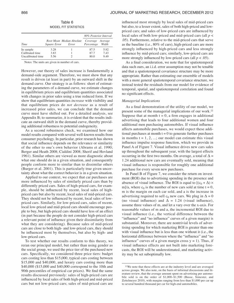
However, our theory of sales increase is fundamentally ademand-side argument. Therefore, we must show that anyresult is driven (at least in part) by an outward shift in thedemand curve. Our strategy is as follows: short of estimat-ing the parameters of a demand curve, we estimate changesin equilibrium prices and equilibrium quantities associatedwith changes in prior sales using a true reduced form. If weshow that equilibrium quantities increase with visibility andthat equilibrium prices do not decrease as a result ofincreased prior sales, we can conclude that the demandcurve must have shifted out. For a detailed analysis, seeAppendix B; to summarize, it is evident that the results indi-cate an outward shift in the demand curve, thereby provid-ing additional robustness to potential endogeneity.
As a second robustness check, we examined how ourmodel results compared with several well-known results fromconsumer psychology. In particular, prior research has shownthat social influence depends on the relevance or similarityof the other to one’s own behavior (Abrams et al. 1990;Berger and Heath 2008; Cialdini 2008; Sherif and Hovland1961). Similar others are viewed as more diagnostic aboutwhat one should do in a given situation, and consequentlypeople conform more to similar than to dissimilar others(Burger et al. 2001). This is particularly true given uncer-tainty about what the correct behavior is in a given situation.
Applied to our context, we expect that car purchases aremore influenced by sales of similarly priced cars than bydifferently priced cars. Sales of high-priced cars, for exam-ple, should be influenced by recent, local sales of high-priced cars but also by recent, local sales of mid-priced cars.They should not be influenced by recent, local sales of low-priced cars. Similarly, for low-priced cars, sales of recent,local low-priced and mid-priced cars should encourage peo-ple to buy, but high-priced cars should have less of an effect(in part because the people do not consider high-priced carsa relevant point of influence given their dissimilarity fromwhat they are considering). Because sales of mid-pricedcars are close to both high- and low-priced cars, they shouldbe influenced most by themselves, but also by high- andlow-priced cars.
To test whether our results conform to this theory, wereran our principal model, but rather than using gender asthe social group, we used the price tier of the purchased newcars. Specifically, we considered three price tiers: budgetcars costing less than $15,000, typical cars costing between$15,000 and $40,000, and luxury cars costing more than$40,000 ($15,000 and $40,000 correspond to the 10th and90th percentiles of empirical car prices). We find the sameresults discussed previously: sales of high-priced cars areinfluenced by local sales of both high-priced and mid-pricedcars but not low-priced cars; sales of mid-priced cars are
influenced most strongly by local sales of mid-priced carsbut also, to a lesser extent, sales of both high-priced and low-priced cars; and sales of low-priced cars are influenced bylocal sales of both low-priced and mid-priced cars (all p <.05). Furthermore, relative to the mid-priced cars that serveas the baseline (i.e., 80% of cars), high-priced cars are morestrongly influenced by high-priced cars and less stronglyinfluence by mid-priced cars; similarly, low-priced cars aremore strongly influenced by low-priced cars (all p < .05).
As a final consideration, we note that for spatiotemporaldata such ours, an i.i.d. error assumption may not be tenableand that a spatiotemporal covariance structure may be moreappropriate. Rather than estimating our ensemble of modelswith a more general spatiotemporal covariance structure, weinstead tested the residuals from our model for evidence oftemporal, spatial, and spatiotemporal correlation and foundno significant effects. Managerial Implications
As a final demonstration of the utility of our model, wepresent some of the managerial implications of our work.11Suppose that at month t = 0, a firm engages in additionaladvertising that leads to four additional women and fouradditional men purchasing automobiles. If visual influenceaffects automobile purchases, we would expect these addi-tional purchases at month t = 0 to generate further purchasesin months t = 1, 2, ...; our model can estimate this visualinfluence impulse response function, which we provide inPanel A of Figure 7. Visual influence drives new cars salesup throughout the subsequent year, with the largest effectsoccurring in the first two months. On average, a total of Δ =1.24 additional new cars are eventually sold, meaning thatvisual influence is responsible for roughly one additionalpurchase for every seven new purchases.
In Panel B of Figure 7, we consider the return on invest-ment (ROI) due to advertising spending in the presence andabsence of visual influence. The ROI is equal to [(c0 + Δ) ¥m]/a, where c0 is the number of new cars sold at time t = 0,m is the margin on each car sold, and a is the increase inadvertising required to sell c0 new cars. We plug in Δ = 0(no visual influence) and Δ = 1.24 (visual influence),assume three values of m, and let a vary over the x-axis. Forreasonable values of m and a, the incremental ROI due tovisual influence (i.e., the vertical difference between the“influence” and “no influence” curves of a given margin) issubstantial. Moreover, there are nontrivial levels of adver-tising spending for which marketing ROI is greater than onewith visual influence but is less than one without it (i.e., thehorizontal difference between where the “influence” and “noinfluence” curves of a given margin cross y = 1). Thus, ifvisual influence effects are not built into marketing fore-casts, the ROI will be underestimated, and marketing activ-ity may be set suboptimally low.
866 JOURNAL OF MARKETING RESEARCH, DECEMBER 2012
Table 6MODEL FIT STATISTICS
80% Posterior IntervalRoot Mean Median Absolute Coverage Average
Time Square Error Error Percentage WidthIn sample 3.28 1 87.5 5.92Calibrated time 3.83 1 87.7 7.43Uncalibrated time 5.56 2 80.0 9.49
Notes: The units are given in number of cars.
11We note that these effects are at the industry level and are averagedacross groups. We also note, on the basis of informal discussions and lit-erature review, that the average amount spent on advertising per automo-bile sold is on the order of $1,000–$1,500 (Busse, Simester, andZettelmeyer 2010), with margins ranging from less than $1,000 per car upto several hundred thousand per car for high-end automobiles.
H JMR 11 0223 Color Web Layout_JMR (2011 Specs) 11/9/12 11:20 AM Page 866
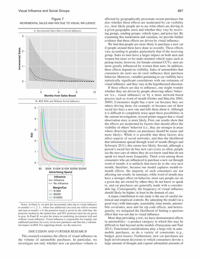
Visual Influence and Social Groups 867
DISCUSSION AND FURTHER RESEARCHThis research examines the effects of visual influence on
the volume of automobile purchases. In particular, weinvestigate not only whether new car purchase volume is
affected by geographically proximate recent purchases butalso whether these effects are moderated by car visibility(i.e., how likely people are to see what others are driving ina given geographic area) and whether they vary by receiv-ing groups, sending groups, vehicle types, and price tier. Byexamining this moderation and variation, we provide furtherevidence that these effects are driven by visual influence.
We find that people are more likely to purchase a new carif people around them have done so recently. These effectsvary according to gender, particularly that of the receivinggroup. Sales to men have a larger impact on both men andwomen but more so for male-oriented vehicle types such aspickup trucks; however, for female-oriented CUVs, men aremore greatly influenced by women than men. In addition,these effects depend on visibility. Sales of automobiles thatconsumers do (not) see do (not) influence their purchasebehavior. Moreover, variables pertaining to car visibility havestatistically significant correlations with our estimates ofvisual influence, and they vary in the hypothesized direction.
If these effects are due to influence, one might wonderwhether they are driven by people observing others’ behav-ior (i.e., visual influence) or by a more network-basedprocess such as word of mouth (Godes and Mayzlin 2004,2009). Consumers might buy a new car because they seeothers driving them, for example, or because one of theirsocial ties buys a new one and tells them about it. Althoughit is difficult to completely tease apart these possibilities inthe current investigation, several points suggest that a visualobservation story is more likely. First, our results show thatthe effects are moderated by factors that should affect thevisibility of others’ behavior (i.e., they are stronger in areaswhere observing others car purchases should be easier andmore likely). While it is possible that these factors alsoaffect aspects of social networks, and thus the likelihoodthat information spread through word of mouth (Berger andSchwartz 2011), this seems less likely. Second, although aperson’s social ties do buy new cars every so often, peoplesee the new cars of others they do not know (and thus do notspeak to) much more frequently. Third, even among thoseconsumers who are influenced to purchase a new car throughword of mouth, it is unlikely that most do so the very nextmonth; therefore, because our model captures month-to-month effects, the majority of such consumers are notaffecting our results. In summary, while word of mouth mayhave a stronger effect on behavior, most cars people see ona given day are owned by others they do not know or speakto, and car purchases are generally made with a consider-able lag. Consequently, the frequency of visual influenceshould likely be higher, at least in the domain of cars.
A major contribution to our study is the use of careful sta-tistical and empirical controls. By saturating the model (in agood way) with intercepts, seasonality, time trends, automo-bile covariates, near and far zip code effects, and hetero-geneity, we mitigated the likelihood of finding a spuriouseffect that was not due to visual influence.
More than providing a test, we have demonstrated effectsin automobiles—a product category in which this may bedifficult to find beyond niche models (Narayanan and Nair2011). Functional considerations play a large role in auto-mobile purchases, as do a variety of constraints (e.g.,budget, prior leases). Furthermore, new car purchases arehigh-involvement decisions to which consumers devote alarge amount of thought and expend substantial amounts of
Figure 7INCREMENTAL SALES AND ROI DUE TO VISUAL INFLUENCE
A: Incremental Sales Due to Social Influence
B: ROI With and Without Social Influence
Notes: In Panel A, we plot the incremental sales due to visual influencein months t = 1, 2, 3... when four additional cars each are sold to womenand men at month t = 0; the posterior mean is given by the solid line, theposterior median by the dashed line, and 95% posterior intervals are givenin gray. In Panel B, we plot the return on marketing investment with andwithout visual influence. Visual influence is responsible for roughly oneadditional purchase for every seven new purchases and thus has a substan-tial impact on ROI. For supporting details, see the main text.
3
2
1
0
Increm
ental S
ales
Months from Sales Boost3 6 9 12
5
4
3
2
1
0
ROI
Advertising Spend$50K$0 $100K $150K $200K $250K
InfluenceInfluenceNo influenceMargin/Car$1000$5000$10000
H JMR 11 0223 Color Web Layout_JMR (2011 Specs) 11/9/12 11:20 AM Page 867
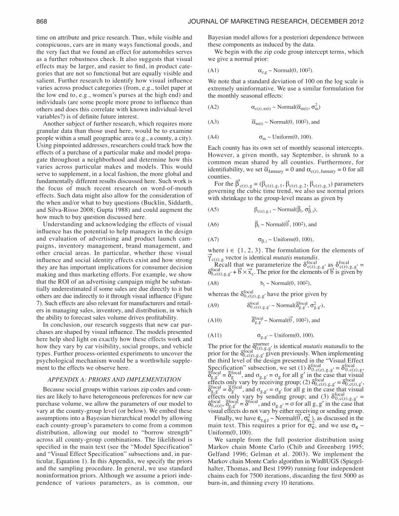
time on attribute and price research. Thus, while visible andconspicuous, cars are in many ways functional goods, andthe very fact that we found an effect for automobiles servesas a further robustness check. It also suggests that visualeffects may be larger, and easier to find, in product cate-gories that are not so functional but are equally visible andsalient. Further research to identify how visual influencevaries across product categories (from, e.g., toilet paper atthe low end to, e.g., women’s purses at the high end) andindividuals (are some people more prone to influence thanothers and does this correlate with known individual-levelvariables?) is of definite future interest.
Another subject of further research, which requires moregranular data than those used here, would be to examinepeople within a small geographic area (e.g., a county, a city).Using pinpointed addresses, researchers could track how theeffects of a purchase of a particular make and model propa-gate throughout a neighborhood and determine how thisvaries across particular makes and models. This wouldserve to supplement, in a local fashion, the more global andfundamentally different results discussed here. Such work isthe focus of much recent research on word-of-moutheffects. Such data might also allow for the consideration ofthe when and/or what to buy questions (Bucklin, Siddarth,and Silva-Risso 2008; Gupta 1988) and could augment thehow much to buy question discussed here.
Understanding and acknowledging the effects of visualinfluence has the potential to help managers in the designand evaluation of advertising and product launch cam-paigns, inventory management, brand management, andother crucial areas. In particular, whether these visualinfluence and social identity effects exist and how strongthey are has important implications for consumer decisionmaking and thus marketing efforts. For example, we showthat the ROI of an advertising campaign might be substan-tially underestimated if some sales are due directly to it butothers are due indirectly to it through visual influence (Figure7). Such effects are also relevant for manufacturers and retail-ers in managing sales, inventory, and distribution, in whichthe ability to forecast sales volume drives profitability.
In conclusion, our research suggests that new car pur-chases are shaped by visual influence. The models presentedhere help shed light on exactly how these effects work andhow they vary by car visibility, social groups, and vehicletypes. Further process-oriented experiments to uncover thepsychological mechanism would be a worthwhile supple-ment to the effects we observe here.
APPENDIX A: PRIORS AND IMPLEMENTATIONBecause social groups within various zip codes and coun-
ties are likely to have heterogeneous preferences for new carpurchase volume, we allow the parameters of our model tovary at the county-group level (or below). We embed theseassumptions into a Bayesian hierarchical model by allowingeach county-group’s parameters to come from a commondistribution, allowing our model to “borrow strength”across all county-group combinations. The likelihood isspecified in the main text (see the “Model Specification”and “Visual Effect Specification” subsections and, in par-ticular, Equation 1). In this Appendix, we specify the priorsand the sampling procedure. In general, we use standardnoninformation priors. Although we assume a priori inde-pendence of various parameters, as is common, our
Bayesian model allows for a posteriori dependence betweenthese components as induced by the data.
We begin with the zip code group intercept terms, whichwe give a normal prior:(A1) az,g ~ Normal(0, 1002).We note that a standard deviation of 100 on the log scale isextremely uninformative. We use a similar formulation forthe monthly seasonal effects:(A2) ac(z), m(t) ~ Normal(am(t), sm
2 )
(A3) am(t) ~ Normal(0, 1002), and
(A4) sm ~ Uniform(0, 100).Each county has its own set of monthly seasonal intercepts.However, a given month, say September, is shrunk to acommon mean shared by all counties. Furthermore, foridentifiability, we set aJanuary = 0 and ac(z), January = 0 for allcounties.
For the bÆc(z), g = (βc(z), g, 1, βc(z), g, 2, βc(z), g, 3) parametersgoverning the cubic time trend, we also use normal priorswith shrinkage to the group-level means as given by (A5) βc(z), g, i ~ Normal(bi, s2
b, i),
(A6) bi ~ Normal(0Æ, 1002), and
(A7) sb, i ~ Uniform(0, 100),where i Œ {1, 2, 3}. The formulation for the elements ofgÆ
c(z), g vector is identical mutatis mutandis.Recall that we parameterize the dfocal
c(z), g, g¢ as dfocalc(z), g, g¢ =
dfocal0,c(z),g,g¢ + bÆ¥ xÆc. The prior for the elements of bÆ is given by
(A8) bi ~ Normal(0, 1002),whereas the dfocal
0, c(z), g, g¢ have the prior given by(A9) dfocal
0, c(z), g, g¢ ~ Normal(dfocalg, g¢ , s2
g, g¢),
(A10) dfocalg, g¢ ~ Normal(0Æ, 1002), and
(A11) sg, g¢ ~ Uniform(0, 100).The prior for the dpartner
c(z), g, g¢ is identical mutatis mutandis to theprior for the dfocal
0, c(z), g, g¢ given previously. When implementingthe third level of the design presented in the “Visual EffectSpecification” subsection, we set (1) dfocal
0, c(z), g, g¢ = dfocal0, c(z), g,
dfocalg, g¢ = dg
focal, and σg, g¢ = σg for all g¢ in the case that visualeffects only vary by receiving group; (2) dfocal
0, c(z),g,g¢ = dfocal0, c(z),g¢,
dfocalg, g¢ = dg¢
focal, and σg,g¢ = σg¢ for all g in the case that visualeffects only vary by sending group; and (3) dfocal
0, c(z), g, g¢ =dfocal
0, c(z), dfocalg, g¢ = dfocal, and σg, g¢ = σ for all g, g¢ in the case that
visual effects do not vary by either receiving or sending group.Finally, we have єz,g,t ~ Normal(0Æ, s2
є, ), as discussed in themain text. This requires a prior for s2
є, and we use sє ~ Uniform(0, 100).
We sample from the full posterior distribution usingMarkov chain Monte Carlo (Chib and Greenberg 1995;Gelfand 1996; Gelman et al. 2003). We implement theMarkov chain Monte Carlo algorithm in WinBUGS (Spiegel -halter, Thomas, and Best 1999) running four independentchains each for 7500 iterations, discarding the first 5000 asburn-in, and thinning every 10 iterations.
868 JOURNAL OF MARKETING RESEARCH, DECEMBER 2012
H JMR 11 0223 Color Web Layout_JMR (2011 Specs) 11/9/12 11:20 AM Page 868
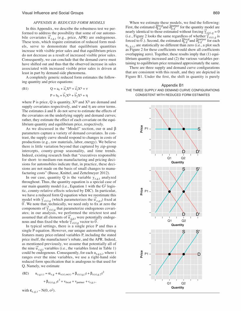
Visual Influence and Social Groups 869
d
d
d
APPENDIX B: REDUCED FORM MODELSIn this Appendix, we describe the robustness test we per-
formed to address the possibility that some of our automo-bile covariates uÆz,g,t (e.g., price, APR) are endogenous.These tests, which require estimation of reduced form mod-els, serve to demonstrate that equilibrium quantitiesincrease with visible prior sales and that equilibrium pricesdo not decrease as a result of increased visible prior sales.Consequently, we can conclude that the demand curve musthave shifted out and thus that the observed increase in salesassociated with increased visible prior sales is driven atleast in part by demand-side phenomena.
A completely generic reduced form estimates the follow-ing quantity and price equations: (B1) Q = a0 + aÆ1XD + aÆ2XS + n
P = b0 + bÆ1XD + bÆ2XS + hwhere P is price, Q is quantity, XD and XS are demand andsupply covariates respectively, and n and h are error terms.The estimates â and b do not serve to estimate the effects ofthe covariates on the underlying supply and demand curves;rather, they estimate the effect of each covariate on the equi-librium quantity and equilibrium price, respectively.
As we discussed in the “Model” section, our a and bparameters capture a variety of demand covariates. In con-trast, the supply curve should respond to changes in costs ofproductions (e.g., raw materials, labor, energy). We believethere is little variation beyond that captured by zip-groupintercepts, county-group seasonality, and time trends.Indeed, existing research finds that “executives responsiblefor short- to medium-run manufacturing and pricing deci-sions for automobiles indicate that, in practice, these deci-sions are not made on the basis of small changes to manu-facturing costs” (Busse, Knittel, and Zettelmeyer 2012).
In our case, quantity Q is the variable yz,g,t analyzedthroughout. Thus, the quantity equation is a special case ofour main quantity model (i.e., Equation 1 with the G2 logis-tic, county-relative effects selected by DIC). In particular,we have a reduced form Q equation when we reestimate thismodel with gÆc(z),g (which parameterizes the uÆz,g,t) fixed at0Æ. We note that, technically, we need only to fix at zero thecomponents of gÆc(z),g that parameterize endogenous covari-ates; in our analysis, we performed the strictest test andassumed that all elements of uÆz,g,t were potentially endoge-nous and thus fixed the whole gÆc(z),g vector to 0Æ.
In typical settings, there is a single price P and thus asingle P equation. However, our unique automobile settingfeatures many price-related variables P, including the statedprice itself, the manufacturer’s rebate, and the APR. Indeed,as mentioned previously, we assume that potentially all ofthe nine uÆz,g,t variables (i.e., the variables listed in Table 1)could be endogenous. Consequently, for each uz,g,t,i, where iranges over the nine variables, we use a right-hand sidereduced form specification that is analogous to that used forQ. Namely, we estimate
with єz, g, t ~ N(0, σ2).
= α + α + β + β
+ β + + +
(B2) u t t
t v v ,z,g,t,i z,g c(z),m(t) c(z),g,1 c(z),g,2
2
c(z),g,33
focal partner z,g, t
When we estimate these models, we find the following:First, the estimated dfocal
g,g¢ and dg,g¢partner for the quantity model are
nearly identical to those estimated without forcing gÆc(z), g = 0(i.e., Figure 2 looks the same regardless of whether gÆc(z), g isforced to 0Æ.). Second, the estimated dfocal
g, g¢ and dg, g¢partner for each
uz, g, t, i are statistically no different than zero (i.e., a plot suchas Figure 2 for these coefficients would show all coefficientsoverlapping zero). Together, these results imply that (1) equi-librium quantity increased and (2) the various variables per-taining to equilibrium price remained approximately the same.
There are three supply and demand curve configurationsthat are consistent with this result, and they are depicted inFigure B1. Under the first, the shift in quantity is purely
l l
D D'
SP1
Price
QuantityQ1 Q2
l l
D D'
S S'
P1
Price
QuantityQ1 Q2
l l D
S S'
P1
Price
QuantityQ1 Q2
Appendix B1THE THREE SUPPLY AND DEMAND CURVE CONFIGURATIONS
CONSISTENT WITH REDUCED FORM ESTIMATES
H JMR 11 0223 Color Web Layout_JMR (2011 Specs) 11/9/12 11:20 AM Page 869

demand driven. Under the second, there are both demandand supply effects. Under the third, there are only supplyeffects. Because we can rule out the third scenario (i.e., ahorizontal demand curve is implausible in the market for allcars), we can confidently conclude that our observed effectsare driven, at least in part, by demand.12
REFERENCESAbrams, Dominic, Margaret Wetherell, Sandra Cochrane, Michael
A. Hogg, and John C. Turner (1990), “Knowing What to Thinkby Knowing Who You Are: Self-Categorization and the Natureof Norm Formation, Conformity and Group Polarization,”British Journal of Social Psychology, 29 (2), 97–119.
Asch, Solomon Eliot (1956), “Studies of Independence and Con-formity: A Minority of One Against a Numerous Majority,” Psy-chological Monographs, 70 (416), 1–70.
Banerjee, Abhijit V. (1992), “A Simple Model of Herd Behavior,”Quarterly Journal of Economics, 107 (3), 797–817.
Banerjee, Sudipto, Bradley P. Carlin, and Alan E. Gelfand (2004),Hierarchical Modeling and Analysis for Spatial Data. BocaRaton, FL: Chapman and Hall/CRC.
Bell, David R. and Sangyoung Song (2007), “Neighborhood Effectsand Trial on the Internet: Evidence from Online Grocery Retail-ing,” Quantitative Marketing and Economics, 5 (4), 361–400.
Bem, Sandra L. (1981), “Gender Schema Theory: A CognitiveAccount of Sex Typing,” Psychological Review, 88 (4), 354–64.
Berger, Jonah and Chip Heath (2007), “Where Consumers Divergefrom Others: Identity-Signaling and Product Domains,” Journalof Consumer Research, 34 (August), 121–34.
——— and ——— (2008), “Who Drives Divergence? Identity Sig-naling, Outgroup Dissimilarity, and the Abandonment of Cul-tural Tastes,” Journal of Personality and Social Psychology, 95(3), 593–607.
——— and Lindsay Rand (2008), “Shifting Signals to Help Health:Using Identity Signaling to Reduce Risky Heath Behaviors,”Journal of Consumer Research, 32 (5), 509–518.
——— and Eric Schwartz (2011), “What Drives Immediate andOngoing Word of Mouth?” Journal of Marketing Research, 48(October), 869–80.
Bikhchandani, Sushil, David Hirshleifer, and Ivo Welch (1992),“A Theory of Fads, Fashion, Custom and Cultural Change asInformational Cascades,” Journal of Political Economy, 100(5), 992–1926.
Brown, Larry, Tony Cai, and Anirban DasGupta (2006), “OnSelecting an Optimal Transformation,” technical report, Univer-sity of Pennsylvania.
Bucklin, Randolph E., Sivaramakrishnan Siddarth, and Jorge M.Silva-Risso (2008), “Distribution Intensity and New CarChoice,” Journal of Marketing Research, 45 (August), 473–86.
Burger, Jerry M., Shelley Soroka, Katrina Gonago, Emily Murphy,and Emily Somervell (2001), “The Effect of Fleeting Attractionon Compliance to Requests,” Personality Social PsychologyBulletin, 27 (12), 1578–86.
Burnkrant, Robert E. and Alain Cousineau (1975), “Informationaland Normative Social Influence in Buyer Behavior,” Journal ofConsumer Research, 2 (3), 206–215.
Busse, Meghan, Christopher R. Knittel, and Florian Zettelmeyer(2012), “Pain at the Pump: The Effect of Gasoline Prices onNew and Used Automobile Markets,” American EconomicReview, forthcoming.
———, Duncan Simester, and Florian Zettelmeyer (2010), “TheBest Price You’ll Ever Get: The 2005 Employee Discount Pric-
ing Promotions in the U.S. Automobile Industry,” MarketingScience, 29 (2), 268–90.
Cai, Hongbin, Yuyu Chen, and Hanming Fang (2009), “Observa-tional Learning: Evidence from a Randomized Natural FieldExperiment,” American Economic Review, 99 (3), 864–82.
Chib, Siddhartha and Edward Greenberg (1994), “Understanding theMetropolis Algorithm,” The American Statistician, 49 (4), 327–35.
Cialdini, Robert B. (2008), Influence: Science and Practice.Boston: Pearson.
DasGupta, Anirban (2008), Asymptotic Theory of Statistics andProbability. New York: Springer.
Dasgupta, Srabana, Sivaramakrishnan Siddarth, and Jorge M.Silva-Risso (2007), “Lease or Buy: A Structural Model of theVehicle Acquisition Decision,” Journal of Marketing Research,44 (August), 490–502.
Deaux, Kay, Anne Reid, Kim Mizrahi, and Kathleen A. Ethier(1995), “Parameters of Social Identity,” Journal of Personalityand Social Psychology, 68 (2), 280–91.
Deutsch, Morton and Harold B. Gerard (1955), “A Study of Nor-mative and Informational Social Influences upon IndividualJudgment,” Journal of Abnormal Psychology, 51 (3), 629–36.
Dubé, Jean-Pierre, Günter J. Hitsch, and Puneet Manchanda(2005), “An Empirical Model of Advertising Dynamics,” Quan-titative Marketing and Economics, 3 (2), 107–144.
Gelfand, Alan E. (1996), “Model Determination Using SamplingBased Methods,” in Markov Chain Monte Carlo in Practice.Boca Raton, FL: Chapman and Hall (CRC), 142–62.
Gelman, Andrew, John B. Carlin, Hal S. Stern, and Donald B.Rubin (2003), Bayesian Data Analysis, 2d ed. Boca Raton, FL:Chapman and Hall/CRC.
Godes, David and Dina Mayzlin (2004), “Using Online Conversa-tions to Study Word-of-Mouth Communication,” Marketing Sci-ence, 23 (4), 545–60.
——— and ——— (2009), “Firm-Created Word-of-Mouth Commu-nication: Evidence from a Field Test,” Marketing Science, 28(4), 721–39.
Grinblatt, Mark, Matti Keloharrju, and Seppo Ikaheimo (2008),“Social Influence and Consumption: Evidence from the Auto-mobile Purchases of Neighbors,” The Review of Economics andStatistics, 90 (4), 735–53.
Gupta, Sunil (1988), “Impact of Sales Promotions on When, What,and How Much to Buy,” Journal of Marketing Research, 25(November), 342–55.
Heffetz, Ori (2011), “A Test of Conspicuous Consumption: Visi-bility and Income Elasticities,” Review of Economics and Statis-tics, 93 (4), 1101–1117.
Johansson, Johny K. (1973), “A Generalized Logistic Functionwith an Application to the Effect of Advertising,” Journal of theAmerican Statistical Association, 68 (344), 824–27.
Joshi, Yogesh V., David J. Reibstein, and Z. John Zhang (2009),“Optimal Entry Timing in Markets with Social Influence,” Man-agement Science, 55 (6), 926–39.
Laurent, Gilles, Jean-Noel Kapferer, and Françoise Roussel(1995), “The Underlying Structure of Brand Awareness Scores,”Marketing Science, 14 (3), G170–G179.
Lenk, Peter J., Wayne S. DeSarbo, Paul E. Green, and Martin R.Young (1996), “Hierarchical Bayes Conjoint Analysis: Recov-ery of Partworth Heterogeneity from Reduced ExperimentalDesigns,” Marketing Science, 15 (2), 173–91.
Manski, Charles F. (1993), “Identification of Endogenous SocialEffects: The Reflection Problem,” Review of Economic Studies,60 (3), 531–42.
Narayanan, Sridhar and Harikesh S. Nair (2011), “Estimating CausalInstalled-Base Effects: A Bias-Correction Approach,” technicalreport, Stanford University Graduate School of Business.
Rossi, Peter E., Greg M. Allenby, and Rob McCulloch (2003),“Bayesian Statistics and Marketing,” Marketing Science, 22 (3),304–328.
870 JOURNAL OF MARKETING RESEARCH, DECEMBER 2012
12We caution the reader not to interpret the visibility finding as necessar-ily arising solely from a shift in the demand curve. While this is one possi-bility, our results are also consistent with shifts in both the demand andsupply curves.
H JMR 11 0223 Color Web Layout_JMR (2011 Specs) 11/9/12 11:20 AM Page 870
Visual Influence and Social Groups 871
Scott-Morton, Fiona, Florian Zettelmeyer, and Jorge Silva-Risso(2001), “Internet Car Retailing,” Journal of Industrial Econom-ics, 49 (4), 501–519.
———, ———, and ——— (2003), “Consumer Information andPrice Discrimination: Does the Internet Affect the Pricing ofNew Cars to Women and Minorities?” Quantitative Marketingand Economics, 1 (1), 65–92.
Shang, Jen, Americus Reed II, and Rachael Croson (2008), “Iden-tity Congruency Effects on Donations,” Journal of MarketingResearch, 45 (June), 351–61.
Sherif, Muzafer and Carl I. Hovland (1961), Social Judgment:Assimilation and Contrast Effects in Communication and Atti-tude Change. New Haven, CT: Yale University Press.
Shriver, Scott K. (2010), “Network Effects in Alternative FuelAdoption: Empirical Analysis of the Market for Ethanol,” tech-nical report, Stanford University Graduate School of Business.
Silva-Risso, Jorge and Irina Ionova (2008), “A Nested LogitModel of Product and Transaction-Type Choice for PlanningAutomakers’ Pricing and Promotions,” Marketing Science, 27(4), 545–66.
Simmel, Georg (1908), “Fashion,” International Quarterly, 10(1),130–35.
Spiegelhalter, David J., Nicola G. Best, Bradley P. Carlin, andAngelika van der Linde (2002), “Bayesian Measures of ModelComplexity and Fit,” Journal of the Royal Statistical Society:Series B (Statistical Methodology), 64 (4), 583–639.
———, Andrew Thomas, and Nicky G. Best (1999), WinBUGSVersion 1.2 User Manual. Cambridge, UK: MRC BiostatisticsUnit.
Srinivasan, Shuba, Koen Pauwels, Jorge M. Silva-Risso, andDominique M. Hanssens (2004), “Product Innovations, Promo-tions, and Long-Term Firm Value,” Journal of Marketing, 68(October),142–56.
Van den Bulte, Christophe and Yogesh V. Joshi (2007), “NewProduct Diffusion with Influentials and Imitators,” MarketingScience, 26 (3), 400–421.
——— and Gary Lilien (2001), “Medical Innovation Revisited:Social Contagion Versus Marketing Effort,” American Journalof Sociology, 106 (5), 1409–1435.
White, Katherine and Darren Dahl (2006), “To Be or Not Be? TheInfluence of Dissociative Reference Groups on Consumer Pref-erences,” Journal of Consumer Psychology, 16 (4), 404–414.
——— and ——— (2007), “Are All Outgroups Created Equal? Con-sumer Identity and Dissociative Influence,” Journal of Con-sumer Research, 34 (4), 525–36.
H JMR 11 0223 Color Web Layout_JMR (2011 Specs) 11/9/12 11:20 AM Page 871