Visual Object Tracking using Adaptive Correlation Filters

David S. Bolme J. Ross Beveridge Bruce A. Draper Yui Man LuiComputer Science Department

Colorado State UniversityFort Collins, CO 80521, USA

bolme@cs.colostate.edu

Abstract

Although not commonly used, correlation filters can trackcomplex objects through rotations, occlusions and otherdistractions at over 20 times the rate of current state-of-the-art techniques. The oldest and simplest correlationfilters use simple templates and generally fail when ap-plied to tracking. More modern approaches such as ASEFand UMACE perform better, but their training needs arepoorly suited to tracking. Visual tracking requires robustfilters to be trained from a single frame and dynamicallyadapted as the appearance of the target object changes.

This paper presents a new type of correlation filter, aMinimum Output Sum of Squared Error (MOSSE) filter,which produces stable correlation filters when initializedusing a single frame. A tracker based upon MOSSE fil-ters is robust to variations in lighting, scale, pose, andnon-rigid deformations while operating at 669 frames persecond. Occlusion is detected based upon the peak-to-sidelobe ratio, which enables the tracker to pause and re-sume where it left off when the object reappears.

Note: This paper contains additional figures and con-

tent that was excluded from CVPR 2010 to meet length

requirements.

1 Introduction

Visual tracking has many practical applications in videoprocessing. When a target is located in one frame ofa video, it is often useful to track that object in subse-quent frames. Every frame in which the target is success-fully tracked provides more information about the identityand the activity of the target. Because tracking is easierthan detection, tracking algorithms can use fewer compu-tational resources than running an object detector on everyframe.

Visual tracking has received much attention in recent

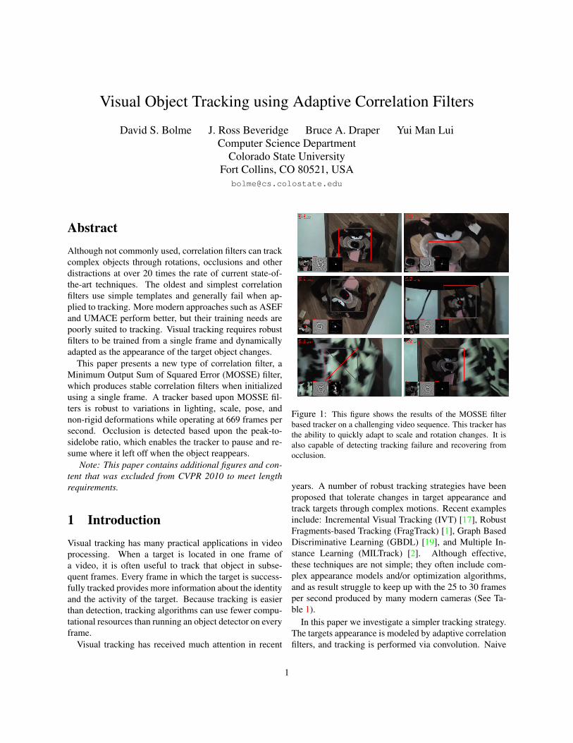
Figure 1: This figure shows the results of the MOSSE filterbased tracker on a challenging video sequence. This tracker hasthe ability to quickly adapt to scale and rotation changes. It isalso capable of detecting tracking failure and recovering fromocclusion.

years. A number of robust tracking strategies have beenproposed that tolerate changes in target appearance andtrack targets through complex motions. Recent examplesinclude: Incremental Visual Tracking (IVT) [17], RobustFragments-based Tracking (FragTrack) [1], Graph BasedDiscriminative Learning (GBDL) [19], and Multiple In-stance Learning (MILTrack) [2]. Although effective,these techniques are not simple; they often include com-plex appearance models and/or optimization algorithms,and as result struggle to keep up with the 25 to 30 framesper second produced by many modern cameras (See Ta-ble 1).

In this paper we investigate a simpler tracking strategy.The targets appearance is modeled by adaptive correlationfilters, and tracking is performed via convolution. Naive

1

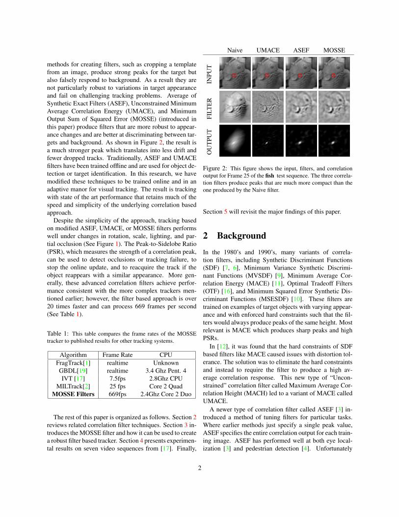
methods for creating filters, such as cropping a templatefrom an image, produce strong peaks for the target butalso falsely respond to background. As a result they arenot particularly robust to variations in target appearanceand fail on challenging tracking problems. Average ofSynthetic Exact Filters (ASEF), Unconstrained MinimumAverage Correlation Energy (UMACE), and MinimumOutput Sum of Squared Error (MOSSE) (introduced inthis paper) produce filters that are more robust to appear-ance changes and are better at discriminating between tar-gets and background. As shown in Figure 2, the result isa much stronger peak which translates into less drift andfewer dropped tracks. Traditionally, ASEF and UMACEfilters have been trained offline and are used for object de-tection or target identification. In this research, we havemodified these techniques to be trained online and in anadaptive manor for visual tracking. The result is trackingwith state of the art performance that retains much of thespeed and simplicity of the underlying correlation basedapproach.

Despite the simplicity of the approach, tracking basedon modified ASEF, UMACE, or MOSSE filters performswell under changes in rotation, scale, lighting, and par-tial occlusion (See Figure 1). The Peak-to-Sidelobe Ratio(PSR), which measures the strength of a correlation peak,can be used to detect occlusions or tracking failure, tostop the online update, and to reacquire the track if theobject reappears with a similar appearance. More gen-erally, these advanced correlation filters achieve perfor-mance consistent with the more complex trackers men-tioned earlier; however, the filter based approach is over20 times faster and can process 669 frames per second(See Table 1).

Table 1: This table compares the frame rates of the MOSSEtracker to published results for other tracking systems.

Algorithm Frame Rate CPUFragTrack[1] realtime UnknownGBDL[19] realtime 3.4 Ghz Pent. 4IVT [17] 7.5fps 2.8Ghz CPU

MILTrack[2] 25 fps Core 2 QuadMOSSE Filters 669fps 2.4Ghz Core 2 Duo

The rest of this paper is organized as follows. Section 2reviews related correlation filter techniques. Section 3 in-troduces the MOSSE filter and how it can be used to createa robust filter based tracker. Section 4 presents experimen-tal results on seven video sequences from [17]. Finally,

Naive UMACE ASEF MOSSE

INPU

TFI

LTER

OU

TPU

T

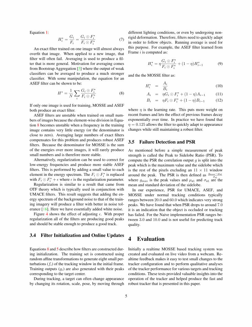
Figure 2: This figure shows the input, filters, and correlationoutput for Frame 25 of the fish test sequence. The three correla-tion filters produce peaks that are much more compact than theone produced by the Naive filter.

Section 5 will revisit the major findings of this paper.

2 Background

In the 1980’s and 1990’s, many variants of correla-tion filters, including Synthetic Discriminant Functions(SDF) [7, 6], Minimum Variance Synthetic Discrimi-nant Functions (MVSDF) [9], Minimum Average Cor-relation Energy (MACE) [11], Optimal Tradeoff Filters(OTF) [16], and Minimum Squared Error Synthetic Dis-criminant Functions (MSESDF) [10]. These filters aretrained on examples of target objects with varying appear-ance and with enforced hard constraints such that the fil-ters would always produce peaks of the same height. Mostrelevant is MACE which produces sharp peaks and highPSRs.

In [12], it was found that the hard constraints of SDFbased filters like MACE caused issues with distortion tol-erance. The solution was to eliminate the hard constraintsand instead to require the filter to produce a high av-erage correlation response. This new type of “Uncon-strained” correlation filter called Maximum Average Cor-relation Height (MACH) led to a variant of MACE calledUMACE.

A newer type of correlation filter called ASEF [3] in-troduced a method of tuning filters for particular tasks.Where earlier methods just specify a single peak value,ASEF specifies the entire correlation output for each train-ing image. ASEF has performed well at both eye local-ization [3] and pedestrian detection [4]. Unfortunately

2

in both studies ASEF required a large number of train-ing images, which made it too slow for visual tracking.This paper reduces this data requirement by introducinga regularized variant of ASEF that is suitable for visualtracking.

3 Correlation Filter Based Tracking

Filter based trackers model the appearance of objects us-ing filters trained on example images. The target is ini-tially selected based on a small tracking window cen-tered on the object in the first frame. From this point on,tracking and filter training work together. The target istracked by correlating the filter over a search window innext frame; the location corresponding to the maximumvalue in the correlation output indicates the new positionof the target. An online update is then performed basedon that new location.

To create a fast tracker, correlation is computed in theFourier domain Fast Fourier Transform (FFT) [15]. First,the 2D Fourier transform of the input image: F = F(f),and of the filter: H = F(h) are computed. The Convolu-tion Theorem states that correlation becomes an element-wise multiplication in the Fourier domain. Using the ⊙symbol to explicitly denote element-wise multiplicationand ∗ to indicate the complex conjugate, correlation takesthe form:

G = F ⊙H∗ (1)

The correlation output is transformed back into the spa-tial domain using the inverse FFT. The bottleneck in thisprocess is computing the forward and inverse FFTs so thatthe entire process has an upper bound time of O(P logP )where P is the number of pixels in the tracking window.

In this section, we discuss the components of filterbased trackers. Section 3.1 discusses preprocessing per-formed on the tracking window. Section 3.2 introducesMOSSE filters which are an improved way to constructa stable correlation filter from a small number of images.Section 3.3 shows how regularization can be used to pro-duce more stable UMACE and ASEF filters. Section 3.4discusses the simple strategy used for the online update ofthe filters.

3.1 Preprocessing

One issue with the FFT convolution algorithm is that theimage and the filter are mapped to the topological struc-ture of a torus. In other words, it connects the left edgeof the image to the right edge, and the top to the bottom.During convolution, the images rotate through the toroidal

space instead of translating as they would in the spatial do-main. Artificially connecting the boundaries of the imageintroduces an artifact which effects the correlation output.

This effect is reduced by following the preprocessingsteps outlined in [3]. First, the pixel values are trans-formed using a log function which helps with low con-trast lighting situations. The pixel values are normalizedto have a mean value of 0.0 and a norm of 1.0. Finally, theimage is multiplied by a cosine window which graduallyreduces the pixel values near the edge to zero. This alsohas the benefit that it puts more emphasis near the centerof the target.

3.2 MOSSE Filters

MOSSE is an algorithm for producing ASEF-like filtersfrom fewer training images. To start, it needs a set of train-ing images fi and training outputs gi. Generally, gi cantake any shape. In this case, gi is generated from groundtruth such that it has a compact (σ = 2.0) 2D Gaussianshaped peak centered on the target in training image fi.Training is conducted in the Fourier domain to take ad-vantage of the simple element-wise relationship betweenthe input and the output. As in the previous section, wedefine the upper case variables Fi, Gi and the filter H tobe the Fourier transform of their lower case counterparts.

H∗i=

Gi

Fi

(2)

where the division is performed element-wise.To find a filter that maps training inputs to the desired

training outputs, MOSSE finds a filter H that minimizesthe sum of squared error between the actual output ofthe convolution and the desired output of the convolution.This minimization problem takes the form:

minH∗

�

i

|Fi ⊙H∗ −Gi|2 (3)

The idea of minimizing Sum of Squared Error (SSE)over the output is not new. In fact, the optimization prob-lem in Equation 3 is almost identical to optimization prob-lems presented in [10] and [12]. The difference is thatin those works it was assumed that the target was alwayscarefully centered in fi and that the output (gi) was fixedfor the entire training set, whereas customizing every giis a fundamental idea behind ASEF and MOSSE. In thetracking problem the target is not always centered, and thepeak in gi moves to follow the target in fi. In a more gen-eral case gi can have any shape. For example, in [4] ficontains multiple targets and gi has multiple correspond-ing peaks.

3

05

1015

2025

3035

Initialization Quality − dudek

Initial Frame Perturbations

Seco

nd F

ram

e PS

R

1 2 4 8 16 32 64 128 256

MOSSEASEFUMACE

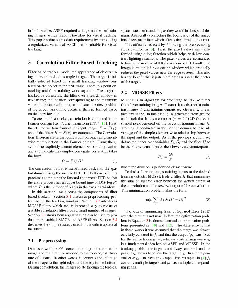
Figure 3: Results shown without regularization.

Solving this optimization problem is not particularlydifficult but does require some care because the functionbeing optimized is a real valued function of a complexvariable. First, each element of H (indexed by ω and ν)can be solved for independently because all operations inthe Fourier domain are performed element-wise. This in-volves rewriting the function in terms of both Hων andH∗

ων. Then, the partial W.R.T. H∗

ωνis set equal to zero,

while treating Hων as an independent variable [13].

0 =∂

∂H∗ων

�

i

|FiωνH∗ων

−Giων |2 (4)

By solving for H∗ a closed form expression for theMOSSE filter is found:

H∗ =

�iGi ⊙ F ∗

i�iFi ⊙ F ∗

i

(5)

A complete derivation is in Appendix A. The terms inEquation 5 have an interesting interpretation. The numer-ator is the correlation between the input and the desiredoutput and the denominator is the energy spectrum of theinput.

From Equation 5, we can easily show that UMACEis a special case of MOSSE. UMACE is defined asH∗ = D−1m∗ where m is a vector containing the FFTof the average centered cropped training images, and D isa diagonal matrix containing the average energy spectrumof the training images [18]. Because D is a diagonal ma-trix, multiplication by its inverse essentially performs an

510

1520

Initialization Quality − dudek

Regularization Parameter

Seco

nd F

ram

e PS

R

0.0001 0.001 0.01 0.1 1.0 10.0

MOSSEASEFUMACE

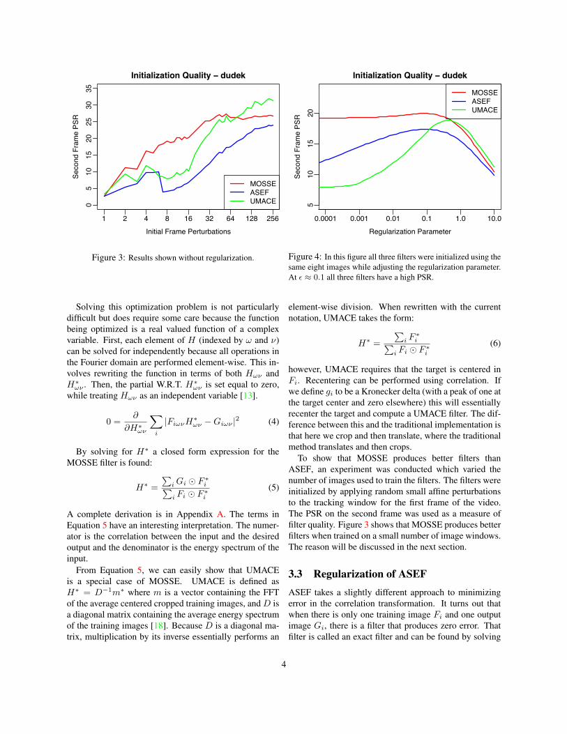
Figure 4: In this figure all three filters were initialized using thesame eight images while adjusting the regularization parameter.At � ≈ 0.1 all three filters have a high PSR.

element-wise division. When rewritten with the currentnotation, UMACE takes the form:

H∗ =

�iF ∗i�

iFi ⊙ F ∗

i

(6)

however, UMACE requires that the target is centered inFi. Recentering can be performed using correlation. Ifwe define gi to be a Kronecker delta (with a peak of one atthe target center and zero elsewhere) this will essentiallyrecenter the target and compute a UMACE filter. The dif-ference between this and the traditional implementation isthat here we crop and then translate, where the traditionalmethod translates and then crops.

To show that MOSSE produces better filters thanASEF, an experiment was conducted which varied thenumber of images used to train the filters. The filters wereinitialized by applying random small affine perturbationsto the tracking window for the first frame of the video.The PSR on the second frame was used as a measure offilter quality. Figure 3 shows that MOSSE produces betterfilters when trained on a small number of image windows.The reason will be discussed in the next section.

3.3 Regularization of ASEF

ASEF takes a slightly different approach to minimizingerror in the correlation transformation. It turns out thatwhen there is only one training image Fi and one outputimage Gi, there is a filter that produces zero error. Thatfilter is called an exact filter and can be found by solving

4

Equation 1:

H∗i=

Gi

Fi

=Gi ⊙ F ∗

i

Fi ⊙ F ∗i

(7)

An exact filter trained on one image will almost alwaysoverfit that image. When applied to a new image, thatfilter will often fail. Averaging is used to produce a fil-ter that is more general. Motivation for averaging comesfrom Bootstrap Aggregation [5] where the output of weakclassifiers can be averaged to produce a much strongerclassifier. With some manipulation, the equation for anASEF filter can be shown to be:

H∗ =1

N

�

i

Gi ⊙ F ∗i

Fi ⊙ F ∗i

(8)

If only one image is used for training, MOSSE and ASEFboth produce an exact filter.

ASEF filters are unstable when trained on small num-bers of images because the element-wise division in Equa-tion 8 becomes unstable when a frequency in the trainingimage contains very little energy (or the denominator isclose to zero). Averaging large numbers of exact filterscompensates for this problem and produces robust ASEFfilters. Because the denominator for MOSSE is the sumof the energies over more images, it will rarely producesmall numbers and is therefore more stable.

Alternatively, regularization can be used to correct forlow-energy frequencies and produce more stable ASEFfilters. This is performed by adding a small value to eachelement in the energy spectrum. The Fi ⊙ F ∗

iis replaced

with Fi ⊙ F ∗i+ � where � is the regularization parameter.

Regularization is similar to a result that came fromOTF theory which is typically used in conjunction withUMACE filters. This result suggests that adding the en-ergy spectrum of the background noise to that of the train-ing imagery will produce a filter with better in noise tol-erance [16]. Here we have essentially added white noise.

Figure 4 shows the effect of adjusting �. With properregularization all of the filters are producing good peaksand should be stable enough to produce a good track.

3.4 Filter Initialization and Online Updates

Equations 8 and 5 describe how filters are constructed dur-ing initialization. The training set is constructed usingrandom affine transformations to generate eight small per-turbations (fi) of the tracking window in the initial frame.Training outputs (gi) are also generated with their peakscorresponding to the target center.

During tracking, a target can often change appearanceby changing its rotation, scale, pose, by moving through

different lighting conditions, or even by undergoing non-rigid deformation. Therefore, filters need to quickly adaptin order to follow objects. Running average is used forthis purpose. For example, the ASEF filter learned fromFrame i is computed as:

H∗i= η

Gi ⊙ F ∗i

Fi ⊙ F ∗i

+ (1− η)H∗i−1 (9)

and the the MOSSE filter as:

H∗i

=Ai

Bi

(10)

Ai = ηGi ⊙ F ∗i+ (1− η)Ai−1 (11)

Bi = ηFi ⊙ F ∗i+ (1− η)Bi−1 (12)

where η is the learning rate. This puts more weight onrecent frames and lets the effect of previous frames decayexponentially over time. In practice we have found thatη = 0.125 allows the filter to quickly adapt to appearancechanges while still maintaining a robust filter.

3.5 Failure Detection and PSR

As mentioned before a simple measurement of peakstrength is called the Peak to Sidelobe Ratio (PSR). Tocompute the PSR the correlation output g is split into thepeak which is the maximum value and the sidelobe whichis the rest of the pixels excluding an 11 × 11 windowaround the peak. The PSR is then defined as gmax−µsl

σsl

where gmax is the peak values and µsl and σsl are themean and standard deviation of the sidelobe.

In our experience, PSR for UMACE, ASEF, andMOSSE under normal tracking conditions typicallyranges between 20.0 and 60.0 which indicates very strongpeaks. We have found that when PSR drops to around 7.0it is an indication that the object is occluded or trackinghas failed. For the Naive implementation PSR ranges be-tween 3.0 and 10.0 and is not useful for predicting trackquality.

4 Evaluation

Initially a realtime MOSSE based tracking system wascreated and evaluated on live video from a webcam. Re-altime feedback makes it easy to test small changes to thetracker configuration and to perform qualitative analysesof the tracker performance for various targets and trackingconditions. These tests provided valuable insights into theoperation of the tracker and helped produce the fast androbust tracker that is presented in this paper.

5

A more controlled evaluation was per-formed on seven commonly used test videoswhich can be freely downloaded fromhttp://www.cs.toronto.edu/∼dross/ivt/.The test videos are all in grayscale and include challeng-ing variations in lighting, pose, and appearance. Thecamera itself is moving in all the videos which adds tothe erratic motion of the targets. The seven sequencesinclude two vehicle tracking scenarios (car4, car11), twotoy tracking scenarios (fish, sylv), and three face trackingscenarios (davidin300, dudek, and trellis70).

4.1 Filter Comparison

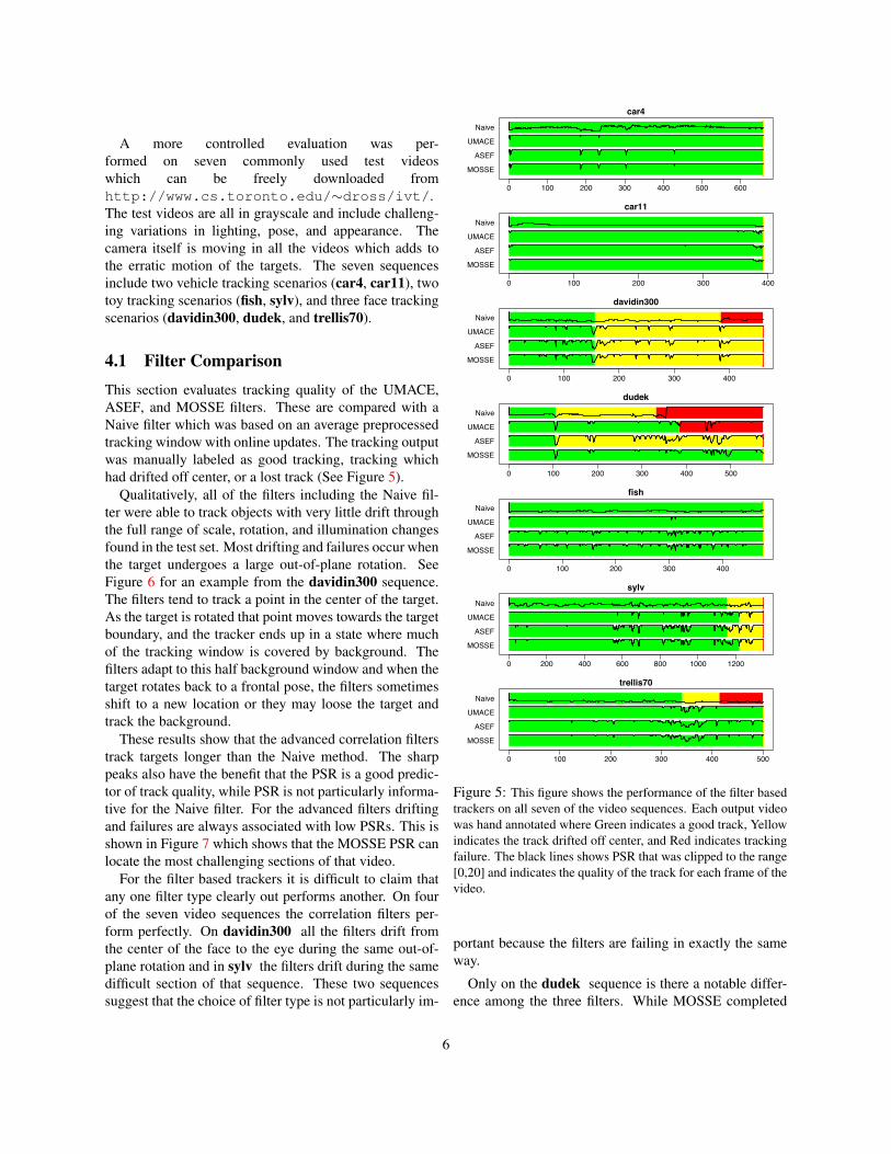
This section evaluates tracking quality of the UMACE,ASEF, and MOSSE filters. These are compared with aNaive filter which was based on an average preprocessedtracking window with online updates. The tracking outputwas manually labeled as good tracking, tracking whichhad drifted off center, or a lost track (See Figure 5).

Qualitatively, all of the filters including the Naive fil-ter were able to track objects with very little drift throughthe full range of scale, rotation, and illumination changesfound in the test set. Most drifting and failures occur whenthe target undergoes a large out-of-plane rotation. SeeFigure 6 for an example from the davidin300 sequence.The filters tend to track a point in the center of the target.As the target is rotated that point moves towards the targetboundary, and the tracker ends up in a state where muchof the tracking window is covered by background. Thefilters adapt to this half background window and when thetarget rotates back to a frontal pose, the filters sometimesshift to a new location or they may loose the target andtrack the background.

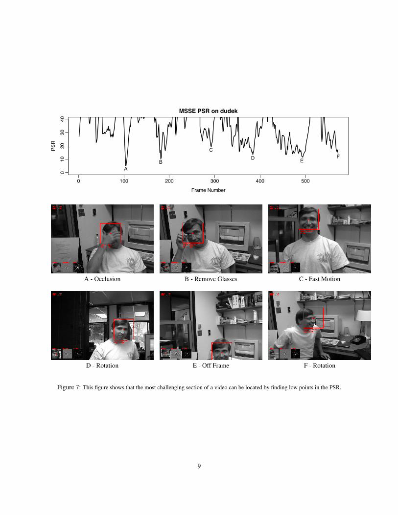
These results show that the advanced correlation filterstrack targets longer than the Naive method. The sharppeaks also have the benefit that the PSR is a good predic-tor of track quality, while PSR is not particularly informa-tive for the Naive filter. For the advanced filters driftingand failures are always associated with low PSRs. This isshown in Figure 7 which shows that the MOSSE PSR canlocate the most challenging sections of that video.

For the filter based trackers it is difficult to claim thatany one filter type clearly out performs another. On fourof the seven video sequences the correlation filters per-form perfectly. On davidin300 all the filters drift fromthe center of the face to the eye during the same out-of-plane rotation and in sylv the filters drift during the samedifficult section of that sequence. These two sequencessuggest that the choice of filter type is not particularly im-

0 100 200 300 400 500 600

car4

MOSSE

ASEF

UMACE

Naive

0 100 200 300 400

car11

MOSSE

ASEF

UMACE

Naive

0 100 200 300 400

davidin300

MOSSE

ASEF

UMACE

Naive

0 100 200 300 400 500

dudek

MOSSE

ASEF

UMACE

Naive

0 100 200 300 400

fish

MOSSE

ASEF

UMACE

Naive

0 200 400 600 800 1000 1200

sylv

MOSSE

ASEF

UMACE

Naive

0 100 200 300 400 500

trellis70

MOSSE

ASEF

UMACE

Naive

Figure 5: This figure shows the performance of the filter basedtrackers on all seven of the video sequences. Each output videowas hand annotated where Green indicates a good track, Yellowindicates the track drifted off center, and Red indicates trackingfailure. The black lines shows PSR that was clipped to the range[0,20] and indicates the quality of the track for each frame of thevideo.

portant because the filters are failing in exactly the sameway.

Only on the dudek sequence is there a notable differ-ence among the three filters. While MOSSE completed

6

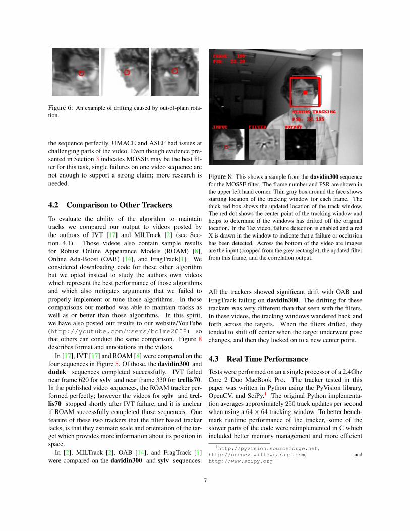
Figure 6: An example of drifting caused by out-of-plain rota-tion.

the sequence perfectly, UMACE and ASEF had issues atchallenging parts of the video. Even though evidence pre-sented in Section 3 indicates MOSSE may be the best fil-ter for this task, single failures on one video sequence arenot enough to support a strong claim; more research isneeded.

4.2 Comparison to Other Trackers

To evaluate the ability of the algorithm to maintaintracks we compared our output to videos posted bythe authors of IVT [17] and MILTrack [2] (see Sec-tion 4.1). Those videos also contain sample resultsfor Robust Online Appearance Models (ROAM) [8],Online Ada-Boost (OAB) [14], and FragTrack[1]. Weconsidered downloading code for these other algorithmbut we opted instead to study the authors own videoswhich represent the best performance of those algorithmsand which also mitigates arguments that we failed toproperly implement or tune those algorithms. In thosecomparisons our method was able to maintain tracks aswell as or better than those algorithms. In this spirit,we have also posted our results to our website/YouTube(http://youtube.com/users/bolme2008) sothat others can conduct the same comparison. Figure 8describes format and annotations in the videos.

In [17], IVT [17] and ROAM [8] were compared on thefour sequences in Figure 5. Of those, the davidin300 anddudek sequences completed successfully. IVT failednear frame 620 for sylv and near frame 330 for trellis70.In the published video sequences, the ROAM tracker per-formed perfectly; however the videos for sylv and trel-

lis70 stopped shortly after IVT failure, and it is unclearif ROAM successfully completed those sequences. Onefeature of these two trackers that the filter based trackerlacks, is that they estimate scale and orientation of the tar-get which provides more information about its position inspace.

In [2], MILTrack [2], OAB [14], and FragTrack [1]were compared on the davidin300 and sylv sequences.

Figure 8: This shows a sample from the davidin300 sequencefor the MOSSE filter. The frame number and PSR are shown inthe upper left hand corner. Thin gray box around the face showsstarting location of the tracking window for each frame. Thethick red box shows the updated location of the track window.The red dot shows the center point of the tracking window andhelps to determine if the windows has drifted off the originallocation. In the Taz video, failure detection is enabled and a redX is drawn in the window to indicate that a failure or occlusionhas been detected. Across the bottom of the video are imagesare the input (cropped from the grey rectangle), the updated filterfrom this frame, and the correlation output.

All the trackers showed significant drift with OAB andFragTrack failing on davidin300. The drifting for thesetrackers was very different than that seen with the filters.In these videos, the tracking windows wandered back andforth across the targets. When the filters drifted, theytended to shift off center when the target underwent posechanges, and then they locked on to a new center point.

4.3 Real Time Performance

Tests were performed on an a single processor of a 2.4GhzCore 2 Duo MacBook Pro. The tracker tested in thispaper was written in Python using the PyVision library,OpenCV, and SciPy.1 The original Python implementa-tion averages approximately 250 track updates per secondwhen using a 64 × 64 tracking window. To better bench-mark runtime performance of the tracker, some of theslower parts of the code were reimplemented in C whichincluded better memory management and more efficient

1http://pyvision.sourceforge.net,http://opencv.willowgarage.com, andhttp://www.scipy.org

7

!!!

!

!

!

!!!

!

!

!

!

!!

!

!!

!!

!

!

!!

!!

!

!

!

!

!

!!

!

!

!

!!!!

!

!!!!

!

!

!

!!!

!!

!

!!

!

!

!

!

!

!

!!!

!!!

!

!

!

!

!

!

!

!!!!

!

!!!!

!!

!

!

!

!

!!

!

!!

!!!!

!!

!

!

!!!!

!

!

!!!!

!!

!

!

!

!

!

!!!!!

!

!

!

!!

!

!

!!

!!!!

!

!

!!

!

!

!

!

!!

!

!!!

!!

!!

!

!!!

!

!

!

!

!

!

!

!

!

!

!!

!

!

!

!!!

!

!

!!

!

!

!

!

!

!

!

!!!!!

!!!

16X16 32X32 64X64 128X128 256X256

Track Update Rate − car4

Filter Size

Upd

ates

Per

Sec

ond

030

060

090

012

00

Figure 9: This figure shows the track update rates for variousfilter sizes. The red x’s indicates the rate during initialization.

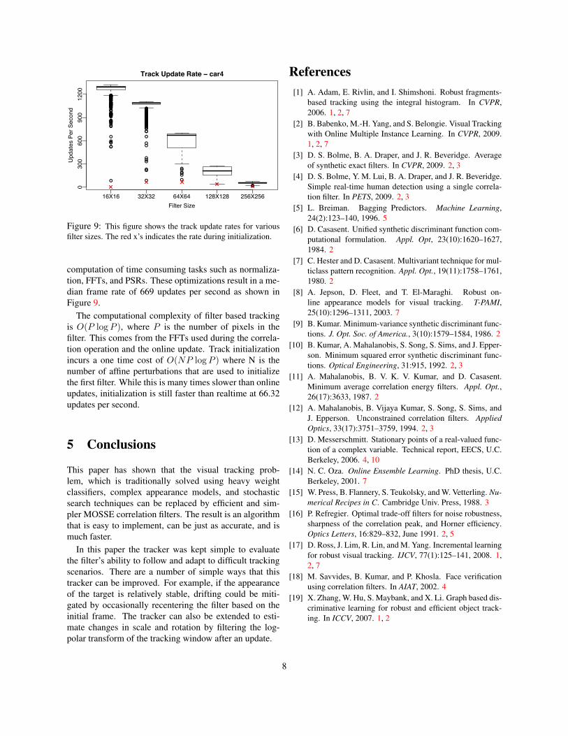
computation of time consuming tasks such as normaliza-tion, FFTs, and PSRs. These optimizations result in a me-dian frame rate of 669 updates per second as shown inFigure 9.

The computational complexity of filter based trackingis O(P logP ), where P is the number of pixels in thefilter. This comes from the FFTs used during the correla-tion operation and the online update. Track initializationincurs a one time cost of O(NP logP ) where N is thenumber of affine perturbations that are used to initializethe first filter. While this is many times slower than onlineupdates, initialization is still faster than realtime at 66.32updates per second.

5 Conclusions

This paper has shown that the visual tracking prob-lem, which is traditionally solved using heavy weightclassifiers, complex appearance models, and stochasticsearch techniques can be replaced by efficient and sim-pler MOSSE correlation filters. The result is an algorithmthat is easy to implement, can be just as accurate, and ismuch faster.

In this paper the tracker was kept simple to evaluatethe filter’s ability to follow and adapt to difficult trackingscenarios. There are a number of simple ways that thistracker can be improved. For example, if the appearanceof the target is relatively stable, drifting could be miti-gated by occasionally recentering the filter based on theinitial frame. The tracker can also be extended to esti-mate changes in scale and rotation by filtering the log-polar transform of the tracking window after an update.

References

[1] A. Adam, E. Rivlin, and I. Shimshoni. Robust fragments-based tracking using the integral histogram. In CVPR,2006. 1, 2, 7

[2] B. Babenko, M.-H. Yang, and S. Belongie. Visual Trackingwith Online Multiple Instance Learning. In CVPR, 2009.1, 2, 7

[3] D. S. Bolme, B. A. Draper, and J. R. Beveridge. Averageof synthetic exact filters. In CVPR, 2009. 2, 3

[4] D. S. Bolme, Y. M. Lui, B. A. Draper, and J. R. Beveridge.Simple real-time human detection using a single correla-tion filter. In PETS, 2009. 2, 3

[5] L. Breiman. Bagging Predictors. Machine Learning,24(2):123–140, 1996. 5

[6] D. Casasent. Unified synthetic discriminant function com-putational formulation. Appl. Opt, 23(10):1620–1627,1984. 2

[7] C. Hester and D. Casasent. Multivariant technique for mul-ticlass pattern recognition. Appl. Opt., 19(11):1758–1761,1980. 2

[8] A. Jepson, D. Fleet, and T. El-Maraghi. Robust on-line appearance models for visual tracking. T-PAMI,25(10):1296–1311, 2003. 7

[9] B. Kumar. Minimum-variance synthetic discriminant func-tions. J. Opt. Soc. of America., 3(10):1579–1584, 1986. 2

[10] B. Kumar, A. Mahalanobis, S. Song, S. Sims, and J. Epper-son. Minimum squared error synthetic discriminant func-tions. Optical Engineering, 31:915, 1992. 2, 3

[11] A. Mahalanobis, B. V. K. V. Kumar, and D. Casasent.Minimum average correlation energy filters. Appl. Opt.,26(17):3633, 1987. 2

[12] A. Mahalanobis, B. Vijaya Kumar, S. Song, S. Sims, andJ. Epperson. Unconstrained correlation filters. Applied

Optics, 33(17):3751–3759, 1994. 2, 3[13] D. Messerschmitt. Stationary points of a real-valued func-

tion of a complex variable. Technical report, EECS, U.C.Berkeley, 2006. 4, 10

[14] N. C. Oza. Online Ensemble Learning. PhD thesis, U.C.Berkeley, 2001. 7

[15] W. Press, B. Flannery, S. Teukolsky, and W. Vetterling. Nu-

merical Recipes in C. Cambridge Univ. Press, 1988. 3[16] P. Refregier. Optimal trade-off filters for noise robustness,

sharpness of the correlation peak, and Horner efficiency.Optics Letters, 16:829–832, June 1991. 2, 5

[17] D. Ross, J. Lim, R. Lin, and M. Yang. Incremental learningfor robust visual tracking. IJCV, 77(1):125–141, 2008. 1,2, 7

[18] M. Savvides, B. Kumar, and P. Khosla. Face verificationusing correlation filters. In AIAT, 2002. 4

[19] X. Zhang, W. Hu, S. Maybank, and X. Li. Graph based dis-criminative learning for robust and efficient object track-ing. In ICCV, 2007. 1, 2

8

0 100 200 300 400 500

010

2030

40

MSSE PSR on dudek

Frame Number

PSR

AB

CD E

F

A - Occlusion B - Remove Glasses C - Fast Motion

D - Rotation E - Off Frame F - Rotation

Figure 7: This figure shows that the most challenging section of a video can be located by finding low points in the PSR.

9

A Minimizing the Output Sum of Squared Error

Here we include a more detailed derivation of the MOSSE process. The paper covers the major steps, and the finalresult. The explanation here shows most of the intermediate steps. The first step in finding a MOSSE filter is to set upthe Minimization problem that will be optimized:

H = minH

�

i

|Fi ⊙H∗ −Gi|2 (13)

Where Fi and Gi are the input images and the corresponding desired outputs in the Fourier domain and goal is to finda filter H that minimizes the sum of squared output error. Because correlation in the Fourier domain is an element-wise multiplication, each element of the filter H can be optimized independently. The optimization problem cantherefore be transformed from a multivariate optimization problem to a problem that optimizes each element of Hindependently.

Hων = minHων

�

i

|FiωνH∗ων

−Giων |2 (14)

where ω and ν index the elements of H .This function is real valued, positive, and convex so it will have only a single optima. Normally to find the optima of

a function, the stable points are found by setting the derivative equal to zero and then solving for the for the variable ofinterest. Finding the stable point for this function is different because it is a real valued function of a complex variable.Care needs to be taken to solve this problem correctly. It turns out that finding the stable points of such a function isnot that difficult. To summarize, it involves rewriting the function in terms of both Hων and H∗

ων. Then, the partial

W.R.T. H∗ων

is set equal to zero, while treating H as an independent variable.

0 =∂

∂H∗ων

�

i

|FiωνH∗ων

−Giων |2 (15)

It can be shown that any Hων which satisfies this equation is a stable point. A short tutorial on this technique can befound in [13]. Transforming this equation leads to:

0 =∂

∂H∗ων

�

i

(FiωνH∗ων

−Giων)(FiωνH∗ων

−Giων)∗ (16)

0 =∂

∂H∗ων

�

i

[(FiωνH∗ων

)(FiωνH∗ων

)∗ − (FiωνH∗ων

)G∗iων

−Giων(FiωνH∗ων

)∗ +GiωνG∗iων

] (17)

0 =∂

∂H∗ων

�

i

FiωνF∗iων

HωνH∗ων

− FiωνG∗iων

H∗ων

− F ∗iων

GiωνHων +GiωνG∗iων

(18)

Computing the partial derivative leads to:

0 =�

i

[FiωνF∗iων

Hων − FiωνG∗iων

] (19)

We can then distribute the summation and solve for Hων .

Hων =

�iFiωνG∗

iων�iFiωνF ∗

iων

(20)

Finally, we rewrite this expression in our original array notation as:

H =

�iFi ⊙G∗

i�iFi ⊙ F ∗

i

(21)

10