Visual Problem Solving with Maple - University of Kentuckycarl/vps98/visualprobs.pdf · 2009-01-08 · Visual Problem Solving with Maple by Paul Eakin, [email protected] and Carl Eberhart,

Visual Problem Solving with Maple

by Paul Eakin, [email protected] and Carl Eberhart, [email protected] of Mathematics, University of Kentucky

First edition June 1997Second Edition January 2009

1

Contents

1 Introduction 51.1 A Lament . . . . . . . . . . . . . . . . . . . . . . . . . . . . . . . . . . . . . . . . . . 51.2 Part of the problem and a remedy . . . . . . . . . . . . . . . . . . . . . . . . . . . . 51.3 Levels of problem solving. . . . . . . . . . . . . . . . . . . . . . . . . . . . . . . . . 71.4 Use of the Maple language and worksheets. . . . . . . . . . . . . . . . . . . . . . . . 9

2 Chapter 1 First steps – Drawing boxes 112.1 What is visual Problem solving? . . . . . . . . . . . . . . . . . . . . . . . . . . . . . 112.2 Mathematical Boxes . . . . . . . . . . . . . . . . . . . . . . . . . . . . . . . . . . . . 112.3 Introductory Exercises: Drawing in the Plane . . . . . . . . . . . . . . . . . . . . . 242.4 More Introductory Exercises and Drawing in Space . . . . . . . . . . . . . . . . . . 27

3 Translating Geometric Objects 303.1 Duplicating and moving cubes . . . . . . . . . . . . . . . . . . . . . . . . . . . . . . . 303.2 The steps in building a cube . . . . . . . . . . . . . . . . . . . . . . . . . . . . . . . . 323.3 Building a TEE . . . . . . . . . . . . . . . . . . . . . . . . . . . . . . . . . . . . . . . 333.4 Exercises: More Pictures in the Plane . . . . . . . . . . . . . . . . . . . . . . . . . . 353.5 Exercises: Making 3d Alphabet Blocks Exercises: Making 3d Alphabet

Blocks . . . . . . . . . . . . . . . . . . . . . . . . . . . . . . . . . . . . . . . . . . . 38

4 Building a Block Factory: Creating a Maple Procedure 414.1 Start with a single cube. . . . . . . . . . . . . . . . . . . . . . . . . . . . . . . . . . . 414.2 Another Example of how to ’procedurize’ ’procedurize’ a sequence of commands 474.3 EXERCISES . . . . . . . . . . . . . . . . . . . . . . . . . . . . . . . . . . . . . . . . 47

5 Laying Bricks:Getting the Computer to do Repetitive Tasks 505.1 Working with expression sequences and lists . . . . . . . . . . . . . . . . . . . . . . . 505.2 How to Build a list by hand . . . . . . . . . . . . . . . . . . . . . . . . . . . . . . . . 515.3 Automatically Generating Sequences and Lists . . . . . . . . . . . . . . . . . . . . . 54

5.3.1 Boring List of Numbers from 672345 To 677345 . . . . . . . . . . . . . . . . . 545.4 Exercises: Sequences and Lists . . . . . . . . . . . . . . . . . . . . . . . . . . . . . . 565.5 Laying bricks. Applications of sequences and lists . . . . . . . . . . . . . . . . . . . 575.6 EXERCISES: Making Brick Patterns With seq . . . . . . . . . . . . . . . . . . . . . 60

6 Stacking Colored Bricks: 616.1 A Chromatic Brick Placer . . . . . . . . . . . . . . . . . . . . . . . . . . . . . . . . . 616.2 Exercises: DO .. OD . . . . . . . . . . . . . . . . . . . . . . . . . . . . . . . . . . . . 636.3 Conditional statements . . . . . . . . . . . . . . . . . . . . . . . . . . . . . . . . . . . 646.4 Exercises: If .. elif .. fi; and if .. else.. fi . . . . . . . . . . . . . . . . . . . . . . . . . 676.5 A vertical chromatic brick placer . . . . . . . . . . . . . . . . . . . . . . . . . . . . . 676.6 Exercises: Colored Brick Stacking . . . . . . . . . . . . . . . . . . . . . . . . . . . . . 69

7 Making it Move - an Introduction to Animations 717.1 Exercises on Movie Making . . . . . . . . . . . . . . . . . . . . . . . . . . . . . . . . 79

2

8 New Problems from Old-A Case Study 818.1 The lawn mowing problem . . . . . . . . . . . . . . . . . . . . . . . . . . . . . . . . 818.2 Visual problems arising from the lawn mowing problem. . . . . . . . . . . . . . . . . 818.3 A specific problem. . . . . . . . . . . . . . . . . . . . . . . . . . . . . . . . . . . . . 85

8.3.1 A lawn mowing word . . . . . . . . . . . . . . . . . . . . . . . . . . . . . . . . 918.3.2 Two Mowers mowing side by side. . . . . . . . . . . . . . . . . . . . . . . . . 928.3.3 Exercises . . . . . . . . . . . . . . . . . . . . . . . . . . . . . . . . . . . . . . 97

9 Mowing Yards (part 2) 999.1 Starting at Different Corners: Going in Different Directions . . . . . . . . . . . . . . 999.2 Sam and Bill Mowing the Same Lawn . . . . . . . . . . . . . . . . . . . . . . . . . . 1029.3 EXERCISES . . . . . . . . . . . . . . . . . . . . . . . . . . . . . . . . . . . . . . . . 111

10 Shadows: Problems from Nature 11410.1 Problems: . . . . . . . . . . . . . . . . . . . . . . . . . . . . . . . . . . . . . . . . . . 11710.2 Moving shadows . . . . . . . . . . . . . . . . . . . . . . . . . . . . . . . . . . . . . . 118

11 More Exercises 11811.1 DIAGRAM CODE . . . . . . . . . . . . . . . . . . . . . . . . . . . . . . . . . . . . . 11911.2 GROUND PLACEMENT . . . . . . . . . . . . . . . . . . . . . . . . . . . . . . . . . 11911.3 Wall Placement . . . . . . . . . . . . . . . . . . . . . . . . . . . . . . . . . . . . . . . 12011.4 PARTIAL STICKPERSON . . . . . . . . . . . . . . . . . . . . . . . . . . . . . . . . 120

12 Pyramids and Prisms 12212.1 Drawing exercises on pyramids. . . . . . . . . . . . . . . . . . . . . . . . . . . . . . . 12212.2 Exercises on prisms . . . . . . . . . . . . . . . . . . . . . . . . . . . . . . . . . . . . . 12312.3 Cross Sections of pyramids and prisms . . . . . . . . . . . . . . . . . . . . . . . . . . 123

13 Cross Sections of triangular prisms 12513.1 The Theorem and its proof. . . . . . . . . . . . . . . . . . . . . . . . . . . . . . . . . 12513.2 A prism with an equilateral base and a 3-4-5 right cross-section . . . . . . . . . . . . 12813.3 EXERCISES . . . . . . . . . . . . . . . . . . . . . . . . . . . . . . . . . . . . . . . . 129

14 Exploring Desargues Theorem. 13014.1 Points and Lines at Infinity . . . . . . . . . . . . . . . . . . . . . . . . . . . . . . . . 13014.2 Exercises On Points and Lines at Infinity . . . . . . . . . . . . . . . . . . . . . . . . 13114.3 Desargues’s Theroem . . . . . . . . . . . . . . . . . . . . . . . . . . . . . . . . . . . . 13214.4 Proof of Desargue’s Theorems . . . . . . . . . . . . . . . . . . . . . . . . . . . . . . . 13514.5 Remarks on Using Desargues Theorem To Represent one Object as a Shadow of

Another . . . . . . . . . . . . . . . . . . . . . . . . . . . . . . . . . . . . . . . . . . . 138

15 The Harmonic rays theorem. 14015.1 A diagram . . . . . . . . . . . . . . . . . . . . . . . . . . . . . . . . . . . . . . . . . 14015.2 PROOF . . . . . . . . . . . . . . . . . . . . . . . . . . . . . . . . . . . . . . . . . . . 14115.3 Exercises . . . . . . . . . . . . . . . . . . . . . . . . . . . . . . . . . . . . . . . . . . 143

3

16 Cross sections of quadrilateral pryamids 14416.1 Exercises . . . . . . . . . . . . . . . . . . . . . . . . . . . . . . . . . . . . . . . . . . 146

17 Mirrors: More Problems from Nature 14717.1 Discussion. . . . . . . . . . . . . . . . . . . . . . . . . . . . . . . . . . . . . . . . . . 147

17.1.1 Diagram ”light1” . . . . . . . . . . . . . . . . . . . . . . . . . . . . . . . . . . 14717.2 Questions: . . . . . . . . . . . . . . . . . . . . . . . . . . . . . . . . . . . . . . . . . 15017.3 Some solutions . . . . . . . . . . . . . . . . . . . . . . . . . . . . . . . . . . . . . . . 15117.4 geombouncer instructions . . . . . . . . . . . . . . . . . . . . . . . . . . . . . . . . . 15617.5 Solution . . . . . . . . . . . . . . . . . . . . . . . . . . . . . . . . . . . . . . . . . . . 160

Index . . . . . . . . . . . . . . . . . . . . . . . . . . . . . . . . . . . . . . . . . . . . . . . . . . . . . . . . . . . . . . . . . . . . . . . . . . . . . . . . . . . . . . .161

4

1 Introduction

1.1 A Lament

Teacher: ”William, you are not doing those additions correctly.”William: ”That,s the way I do them.”

Conversation reported by Dr. Don Coleman when relating his experience as an elementaryschool teacher in 1980

Our Mathematics has been over five millennia in development and is unrivaled among humanconstructions for its unity, consistency, and utility. Nevertheless it is perceived by many as a discon-nected collection of arcane formulas, symbols, and processes whose principal use is the productionof numbers, formulas, or symbols called ’answers’. A ’mathematics problem’ is typically expectedto be stated in a telegraphic style, and produce a single correct answer. The object of mathematicalstudy seems to be learning which steps to apply in a particular situation to produce the answer.Significant weight is attached to the speed and accuracy with which one can produce the answer.’Problems’ tend to be viewed as things found at the end of a chapter or section in a text book or ona test. ’Working a problem’ is a task that takes at most a few minutes of locating a similar exercisein the text and then matching the steps employed to solve that problem to the current problem.The test of whether one’s answer is correct is that it agrees with the table of answers in the backof the book, or the teacher’s answer. Getting the same answer as these oracles 75% of the time isas much as could be expected from an ’average’ student.

Viewed this way William’s approach is altogether reasonable. His algorithm gave the correctsum of three, three digit numbers most of the time. Since mathematics is simply the application ofalgorithms to symbols there was no obvious reason why the official algorithm is preferable to theone he divined and could apply quickly, consistently, and accurately.

There is no report on whether Dr. Coleman’s admonition had an influence on William’s view ofmathematics but as measured by the percentage of college freshmen with the same outlook, over adecade of exposure to the same message, delivered by highly qualified, motivated teachers has notresonated with many. These students, many of whom have made good grades in algorithmic, ’plugand chug’ courses emerge from a dozen year’s study of mathematics with problem solving skillsnot even remotely commensurate with the investment made in their education. Further, they leavewith a view of the discipline and the level to which the average person can master it not so farremoved from that of ancient Egyptians peasants for whom priests reconstructed the boundaries oftheir fields after the floods of the Nile. While obviously imposing career limits on adults who holdthem, such attitudes are readily passed on to the next generation by many parents who are unableto assist and encourage their children in studies of mathematics beyond elementary arithmetic oralgebra.

1.2 Part of the problem and a remedy

William had no objective criterion for assessing whether his solution was better or worse than anyother, other than by comparing it with the ’official’ answer. He could work so fast that he gotmore correct answers than most of his peers so reinforcement from them was unlikely to cause himto re-assess his approach. Nor, one suspects, was input from parents. One may note, however,

5

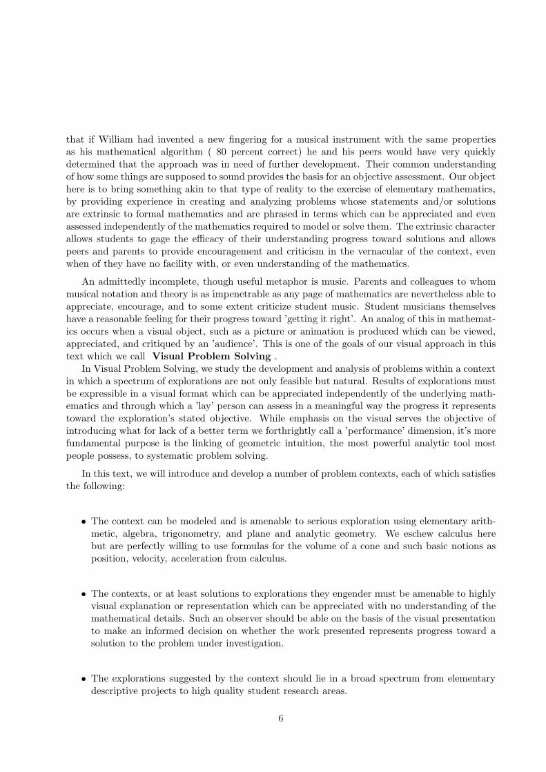
that if William had invented a new fingering for a musical instrument with the same propertiesas his mathematical algorithm ( 80 percent correct) he and his peers would have very quicklydetermined that the approach was in need of further development. Their common understandingof how some things are supposed to sound provides the basis for an objective assessment. Our objecthere is to bring something akin to that type of reality to the exercise of elementary mathematics,by providing experience in creating and analyzing problems whose statements and/or solutionsare extrinsic to formal mathematics and are phrased in terms which can be appreciated and evenassessed independently of the mathematics required to model or solve them. The extrinsic characterallows students to gage the efficacy of their understanding progress toward solutions and allowspeers and parents to provide encouragement and criticism in the vernacular of the context, evenwhen of they have no facility with, or even understanding of the mathematics.

An admittedly incomplete, though useful metaphor is music. Parents and colleagues to whommusical notation and theory is as impenetrable as any page of mathematics are nevertheless able toappreciate, encourage, and to some extent criticize student music. Student musicians themselveshave a reasonable feeling for their progress toward ’getting it right’. An analog of this in mathemat-ics occurs when a visual object, such as a picture or animation is produced which can be viewed,appreciated, and critiqued by an ’audience’. This is one of the goals of our visual approach in thistext which we call Visual Problem Solving .

In Visual Problem Solving, we study the development and analysis of problems within a contextin which a spectrum of explorations are not only feasible but natural. Results of explorations mustbe expressible in a visual format which can be appreciated independently of the underlying math-ematics and through which a ’lay’ person can assess in a meaningful way the progress it representstoward the exploration’s stated objective. While emphasis on the visual serves the objective ofintroducing what for lack of a better term we forthrightly call a ’performance’ dimension, it’s morefundamental purpose is the linking of geometric intuition, the most powerful analytic tool mostpeople possess, to systematic problem solving.

In this text, we will introduce and develop a number of problem contexts, each of which satisfiesthe following:

• The context can be modeled and is amenable to serious exploration using elementary arith-metic, algebra, trigonometry, and plane and analytic geometry. We eschew calculus herebut are perfectly willing to use formulas for the volume of a cone and such basic notions asposition, velocity, acceleration from calculus.

• The contexts, or at least solutions to explorations they engender must be amenable to highlyvisual explanation or representation which can be appreciated with no understanding of themathematical details. Such an observer should be able on the basis of the visual presentationto make an informed decision on whether the work presented represents progress toward asolution to the problem under investigation.

• The explorations suggested by the context should lie in a broad spectrum from elementarydescriptive projects to high quality student research areas.

6

In general our approach is to introduce a context and develop a mathematical model whichcontains or is extensible to a family of explorations. Typically, we initiate a primary investigationand ask students to complete or extend parts of it over a fixed period of time. Except for projectsdone for individual evaluation, students are encouraged to work together in groups. On all projectsstudents are encouraged to confer with faculty frequently on their progress. Modeling the waytechnical investigations develop and proceed in practice, assistance is readily given at the verygeneral conceptual level and the very specific, technical level. In addition, we provide a literatureof investigations which can be used both for general ideas and directions of inquiry.

When the mathematics and vocabulary of a context are well understood, some attention isdirected to its further development/extension through application of some general problem devel-opment techniques. This introduces the art, and science of problem context development in a handson process. The general message is that while new, fruitful problem areas may spring from pureinspiration, by far the largest part of them will be systematically be derived from previous effortsand will inherit many of the features that made the source productive. This is particularly true ofproblem areas ultimately designed for young students - those in which the mathematical prerequi-sites are very modest. We will find that rather than making the development task more difficult,well-chosen constraints such as our ’no calculus’ and the visual requirement for our investigationsprovide both a focus and a wealth of problems to address.

The final stage in the development cycle of a context is the adaptation of its most recent fruitto the classroom. This process is a prism which attempts to carefully resolve the spectrum of (now)well understood possible investigations into a suite of interrelated tasks suitable for individuals orgroups of students of differing levels and interests to pursue with reasonable expectation of success.Student problems will fall into some broad categories:

1.3 Levels of problem solving.

• Exploratory: The development of the problem context produces software (in this case Mapleworksheets) which provide a visual insight into the problem which can be appreciated inde-pendently of the underlying mathematics. These can be developed into student activitieswhich allow them to explore the problem area and gain an appreciation of the question andwhat can be done with the elementary mathematics they are learning.

• Descriptive: At a higher level, students do not simply use the software but modify andextend its geometric content, learning to precisely (mathematically) describe and visuallyrepresent objects in the context. (e.g. polygonal objects, filling in Escher pictures, etc.)

• Manipulative: At a still higher level students not only create visual objects but learn tomanipulate them with mathematics and to represent the results visually. (e.g. translation,dilation).

• Beginning problem solving: A higher level than ”pure” manipulative. Students articulate,solve, and implement visual representation of desired manipulations (e.g. translate/rotate,break apart, etc)

7

• Structured elementary problem solving: These would typically involve a brief sequenceof elementary problem solving steps, with the results of one step needed for another. Problemsare presented in a structured format, typically as extensions of example investigations.

• Elementary Problem Solving: Problems are presented in an open format but withinthe current context. These are typically extensions of example investigations which maybe achieved through different routes. These would be ”straightforward” to the teacher butwould require several hours work for a student or student group to formally ”solve” and anadditional number of hours to complete and prepare a presentation of the solution. Thesegenerally require simplifying assumptions which students should identify and note their rolein the solution.

• Intermediate problem solving: These differ from elementary primarily in the level ofpresentation to the student. They need not fit solely within the current context but should”map” into it with some thought. They may not have been worked in complete detail by theteacher but the former would have a firm conceptual outline of a solution and know that it iswithin the ability of the student. The principal difference between an intermediate problemand an elementary problem is the amount of formal direction given with the problem. Inter-mediate problems should be given with the expectation that even good students will requiresome assistance. This assistance may in total reduce the problem to an elementary problemhad it been given formally, at the outset. However it is given in response to specific studentquestions which reflect work done on the problem and hence is substantially ”generated” bythe student(s).

• Investigative problem solving: This differs from intermediate problem solving in primarilyin the format of the question. Here the teacher knows by experience that the question isreasonable and is confident that he/she can make a contribution. The questions are typicallyphrased as ”What happens if..?”, ”Can this be done if ..?”, etc. Such problems are given tostudents who have successfully completed an intermediate project with some distinction andwho clearly have a ”feel” for the context. Such investigations will often lead to mathematicalproblems well beyond the confines of the elementary model. The identification and clearstatement of such a question, together with numerical/arithmetical or graphical evidencewould be an excellent outcome of such an investigation.

• Advanced problem solving: Students undertake the investigation of a problem whichhas emerged from some of the contexts studied which the teacher knows to be difficult andprobably does not know how to solve or can do so only partially or by employing advancedmathematics. It will often happen that today’s advanced problem is tomorrow’s elementaryproblem - in some sense that conversion is the ultimate goal of the project. Such projectswould be undertaken only by students who have successfully completed an investigative prob-lem solving project and would preferably be done in a mentoring situation with a mathematicsteacher or professor.

8

1.4 Use of the Maple language and worksheets.

Our principal means for integrating images and mathematical symbols and communicating themto others is the computer algebra system Maple. We might just as well have chosen the equallypowerful Mathematica but for the historical fact that when the University of Kentucky first wentlooking for a local computer algebra system Maple offered more attractive terms.

In order to follow this program of study the reader will need access to a current version of Maple.No experience with Maple or any other similar program is assumed. The course materials weredeveloped in Maple V, Release 4 and do take advantage of features such as of that version whichare not available in Release 3. The text was initially developed as a series of Maple V worksheets,and in the current edition as a series of Maple 12 worksheet. While you can read along in the pdfversion, it is recommended that you use the ’book of worksheets’, because you can develop facilitywith Maple more easily that way.

The course materials were developed using computers with Intel Pentium processors, with 16 to32 Mb memory. (My how things have changed). Most of the activities will run quite well on smaller,slower machines but some of them, particularly the three-dimensional animations may be slow orrequire more resources than some of those machines have available. In such cases an understandingof the material will readily allow the user to adapt the material to the local environment.

Since the program Maple is central to this presentation, however our approach we begin witha brief hands-on introduction to a few Maple commands and concepts. These will allow us topromptly begin to use it for our problem solving and communications purposes. As the courseprogresses we will introduce additional tools as they are needed. The reader should immediatelybegin to explore beyond the very limited scope of commands we formally introduce.

Maple material appears in text cells like this one or in in execution cells like the next:> This is an execution cell - you can tell by the ">" prompt. Maple

expectsexpressions entered in at the command prompt to be valid Maple

> commands - which this certainly isn’t. If you press the "enter" keywith the cursor in this cell then Maple will try to interpret it.Since this isn’t a valid command,Maple will return an error message.

Syntax error, missing operator or ‘;‘

In the course of this text we will often discuss words or commands which have meaning to Mapleand will often provide expressions which can be entered at the prompt. One way we can do thisis to provide the input cell with the command already entered, leaving it to the reader to simplypress the ”enter” key to have Maple execute it. For instance:

> 2+7;

9

Note that in such cases we usually leave an empty command line or two. To execute thecommand above one simply places the cursor anywhere in the cell and presses ”enter”. Maple willexecute the command and move the cursor to the next command prompt. If there are many linesof text intervening then the user has to scroll back, and search for the results of the calculation.

In many cases we will not leave commands sitting at command prompts waiting to be inadver-

9

tently executed or modified but will rather place them in the text where the reader can copy theminto a command cell if he/she wishes. Such commands will be recognizable by the font they are inand the fact that they are terminated by a semicolon ”;”. Thus for instance if plot(sin(3*x),x=-Pi..Pi); is copied and pasted into the command line below, an ”enter” will result in a graph ofsin(3x) on the interval [−π, π].

10

2 Chapter 1 First steps – Drawing boxes

2.1 What is visual Problem solving?

Visual problem solving Visual problem solving is concerned with problems whose statementsor solutions (hopefully both) have a visual character which can be appreciated and even assessedwithout reference to the underlying mathematics. This is analogous to the manner in which we canappreciate music without reference to or even understanding of its

creator’s tools - the fact notwithstanding the fact notwithstanding those with suchknowledge can appreciate it at a higher level. In the course of this study we will find that there is anincredible variety of problems of this nature and that there are techniques for developing familiesof them from basic contexts. In this introduction to the subject we will primarily restrict ourattention to problems which can be analyzed with the non-calculus mathematics and basic sciencestudied in middle and high school. However, since part of what we will be doing is generating newproblems from old we must be prepared to find ourselves formulating questions in that vocabularywhose solution requries new tools. We will celebrate when we do for the quest for problems notsolvable within a science is the most basic process in by which it is extended. problem solving isabout marshalling the intellectual tools at our disposal to attack a problem.

The expected result of a serious attack on a problem is a contribution to its solution. Acontribution may well fall short of a complete solution but it will always present one’s formulationof the problem, one’s approach to analyzing the problem, and the results of one’s analysis. Inkeeping with our visual approach at least one of these components components will containelements of a visual nature. In this course our contributions will always take form on a Maple(release 4) worksheet.

Maple is a computer program (sometimes called a symbolic manipulation program) which cangenerate and manipulate algebraic, numerical, and geometric objects. It has a language of its own(the Maple language) through which it can be directed to perform virtually any mathematical orgeometric operation. More over this language is extensible which means that, like any naturallanguage, it can be used to define new words which the program can recognize and new symbolswhich it can manipulate. A Maple Worksheet is an electronic file containing text and insertedimages (which have meaning only to people), Maple commands (words) which direct the programto perform certain operations, and output which is text, images, or other constructs generated bythe program in response to the commands. In general the responses (also called the output) arenot needed if one has the commands since they can always be recovered from the latter. Sucha sequence of commands is typically a small amount of text which can readily be communicatedby electronic mail. This is the form in which all work in this course - all contributions - will bemade, and the primary form of correspondence among the participants in this course. Since this isthe case our first order of business will be to begin to learn how to use Maple as a mathematicalcommunications tool. We learn to do this by doing it. We start with the geometric vocabulary.

2.2 Mathematical Boxes

We assume that the reader is familiar with the fact that any two mutually perpendicular linesin the plane or three mutually perpendicular number lines in space define a cartesian coordinatesystem relative to which every point in the plane or space has a unique name, called its coordinates.

11

Points in the plane or space may have other names such as ”X”,”Lexington”, or ”Detroit”, etc.and for a particular purpose these may be far more descriptive than a list of coordinates. Theimportance of coordinates is that that algebraic relationships among the coordinates of (collectionsof) points fully express geometric relationships among the points themselves. This means that wecan use algebra to express and investigate geometric relationships (and visa versa). Moreover, sincecomputers can ”understand” and ”communicate” algebraic relationships, this provides both a pathto the physical/geometric/visual worlds we propose to explore and a vehicle take us at least partof the way there. The coordinates of a point are a list so our first task is learn about lists in Maple.

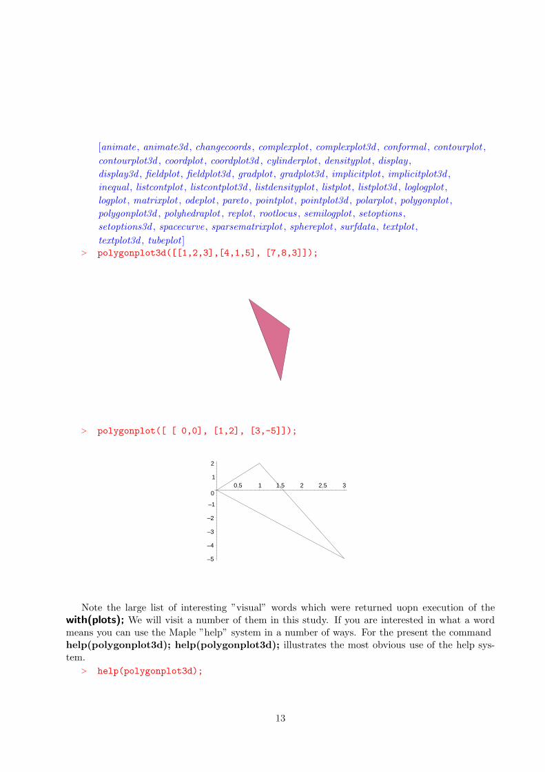
In Maple, lists are sequences of objects enclosed in brackets [ ] . The order of the objects ina list is important. Thus the lists [1,2,3] and [2,1,3] are different and the lists [a,b,c] and [d,e,f] areequal (as lists) only if a=d, b=e, and c=f. Note also that, to Maple, only the first of [1,2,3], {1,2,3},and (1,2,3) is a list. Our initial Maple command to plot points in space is ”plots[polygonplot3d]”which is a command which accepts lists of points and plots the (spatial) polygon with thosepoints as its vertices. Thus if we want to create a visual representation of the spatial trianglewith vertices [1,2,3], [4,1,5] and [7,8,3] we enter the following at the command prompt ”>” .plots[polygonplot3d]([[1,2,3],[4,1,5],[7,8,3]]); plots[polygonplot3d]([[1,2,3],[4,1,5],[7,8,3]]);

The analogous command which displays a polygon in the plane is ”plots[polygonplot].”> plots[polygonplot]([ [ 0,0], [1,2], [3,-5]]);

–5

–4

–3

–2

–1

0

1

2

0.5 1 1.5 2 2.5 3

The ”plots” part of these command tells Maple to look in the ”package” of commands called”plots” for the word polygonplot3d polygonplot3d . We can first tell Maple to ”load” all ofthe words in the plots package into the current session by the command with(plots); after whichit will recognize only the polygonplot3d part.

> with(plots);

12

[animate , animate3d , changecoords , complexplot , complexplot3d , conformal , contourplot ,

contourplot3d , coordplot , coordplot3d , cylinderplot , densityplot , display ,

display3d , fieldplot , fieldplot3d , gradplot , gradplot3d , implicitplot , implicitplot3d ,

inequal , listcontplot , listcontplot3d , listdensityplot , listplot , listplot3d , loglogplot ,

logplot , matrixplot , odeplot , pareto, pointplot , pointplot3d , polarplot , polygonplot ,

polygonplot3d , polyhedraplot , replot , rootlocus , semilogplot , setoptions ,

setoptions3d , spacecurve , sparsematrixplot , sphereplot , surfdata , textplot ,

textplot3d , tubeplot ]> polygonplot3d([[1,2,3],[4,1,5], [7,8,3]]);

> polygonplot([ [ 0,0], [1,2], [3,-5]]);

–5

–4

–3

–2

–1

0

1

2

0.5 1 1.5 2 2.5 3

Note the large list of interesting ”visual” words which were returned uopn execution of thewith(plots); We will visit a number of them in this study. If you are interested in what a wordmeans you can use the Maple ”help” system in a number of ways. For the present the commandhelp(polygonplot3d); help(polygonplot3d); illustrates the most obvious use of the help sys-tem.

> help(polygonplot3d);

13

Although loading the plots package relieves us of a few keystrokes in writing down our workwe will typically forego this for the far greater advantage of portability and readability of ourinstructions. We will continuously find that we want to go back to old worksheets and reuse piecesof code via ”cut and paste” operations. Rather than having to carefully re-read such material tosee if perhaps it depends on packages having been loaded earlier in the worksheet.

The ability of Maple to draw polygons in space provides us with the means to have Maple createimages of any spatial object which consists of polygons. Lets begin with one of the most familiarobjects, a cube. A cube has eight vertices, and six faces, each defined by a sequence of the vertices.Since Maple can work with symbols we can represent the vertices symbolically, say with symbols v1,v2, .. and the faces (top, bottom, left, right, front, and back) as sequences of the vertices. First wesketch our cube, labeling its vertices and faces with these symbols and then ”read off” the lists weneed to communicate with Maple. It is very helpful to use a hand-drawn sketch or diagram. (Youcan draw these with for example ”paint” and cut and paste the sketches into the worksheet.)

ch1vbox

Notice that all of this so far is hand drawings and text. We have not communicated anything tothe Maple program which ”understands” a limited vocabulary and has no ability at all to understandpictures. We enter Maple commands at the command prompt ”>”. We want to describe to Mapleeach of the faces of our box using terms that have meaning (the same meaning) to both us and thecomputer.

Definition: A polygon polygon is an ordered list of points lying in a plane in space.Definition: An n-gon n-gon is a list of n different points. Two lists correspond to the same

polygon if a circular permutation of one or yields the other or a reverse listing of the other.

The connection between our usual geometric view of a polygon and this form is that the listwhich describes it may be thought of as the order in which the verticies are passed as one ”walks”along the boundary of the polygon along a path which passes each vertex exactly once. The factthat there are numerous paths which so this corresponds to the fact that there are numerous listswhich represent a particular polygon. Thus, for instance, the front face of our sketch is the list [v1,v2, v3, v4]. It is also [v2,v3,v4,v1] and [v3, v2,v1,v4].

Problem: Exactly how many different lists of vertices corespond to any one n-gon?It is posible and convenient for the same object to have more than one name in Maple. Thus for

instance, with reference to the above diagram we may want to refer to the ploygon whose verticesare v1,v2,v3,v4 as the ”front face” or simply to give it the name ”front”. Similarly there is a ”back”,”top”, etc, the latter being names for other polygons which are easy to refer to and remember. Theway we tell Maple that we want to refer to the list [v1,v2,v3,v4] as ”face” is via assigned equality.

> front:=[v1,v2,v3,v4];

front := [[2, 0, 3], [2, 1, 3], [2, 1, 2], [2, 0, 2]]

> front;

[[2, 0, 3], [2, 1, 3], [2, 1, 2], [2, 0, 2]]

14

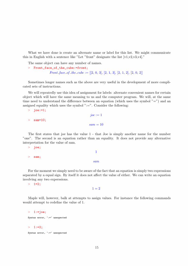
What we have done is create an alternate name or label for this list. We might communicatethis in English with a sentence like ”Let ”front” designate the list [v1,v2,v3,v4].”

The same object can have any number of names.

> Front_face_of_the_cube:=front;

Front face of the cube := [[2, 0, 3], [2, 1, 3], [2, 1, 2], [2, 0, 2]]

Sometimes longer names such as the above are very useful in the development of more compli-cated sets of instructions.

We will repeatedly use this idea of assignment for labels: alternate convenient names for certainobject which will have the same meaning to us and the computer program. We will, at the sametime need to understand the difference between an equation (which uses the symbol ”=”) and anassigned equality which uses the symbol ”:=”. Consider the following:

> joe:=1;

joe := 1

> sam=10;

sam = 10

The first states that joe has the value 1 - that Joe is simply another name for the number”one”. The second is an equation rather than an equality. It does not provide any alternativeinterpretation for the value of sam.

> joe;

1

> sam;

sam

For the moment we simply need to be aware of the fact that an equation is simply two expressionsseparated by a equal sign. By itself it does not affect the value of either. We can write an equationinvolving any two experssions.

> 1=2;

1 = 2

Maple will, however, balk at attempts to assign values. For instance the following commandswould attempt to redefine the value of 1.

> 1:=joe;

Syntax error, ‘:=‘ unexpected

> 1:=2;

Syntax error, ‘:=‘ unexpected

15

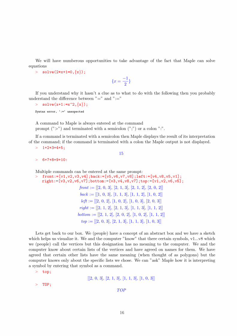
We will have numberous opportunities to take advantage of the fact that Maple can solveequations

> solve(2*x+1=0,{x});

{x =−1

2}

If you understand why it hasn’t a clue as to what to do with the following then you probablyunderstand the difference between ”=” and ”:=”

> solve(x+1:=x^2,{x});Syntax error, ‘:=‘ unexpected

A command to Maple is always entered at the commandprompt (”>”) and terminated with a semicolon (”;”) or a colon ”:”.

If a command is terminated with a semicolon then Maple displays the result of its interpretationof the command; if the command is terminated with a colon the Maple output is not displayed.

> 1+2+3+4+5;

15

> 6+7+8+9+10:

Multiple commands can be entered at the same prompt:> front:=[v1,v2,v3,v4];back:=[v5,v6,v7,v8];left:=[v4,v8,v5,v1];

right:=[v3,v2,v6,v7];bottom:=[v3,v4,v8,v7];top:=[v1,v2,v6,v5];

front := [[2, 0, 3], [2, 1, 3], [2, 1, 2], [2, 0, 2]]

back := [[1, 0, 3], [1, 1, 3], [1, 1, 2], [1, 0, 2]]

left := [[2, 0, 2], [1, 0, 2], [1, 0, 3], [2, 0, 3]]

right := [[2, 1, 2], [2, 1, 3], [1, 1, 3], [1, 1, 2]]

bottom := [[2, 1, 2], [2, 0, 2], [1, 0, 2], [1, 1, 2]]

top := [[2, 0, 3], [2, 1, 3], [1, 1, 3], [1, 0, 3]]

Lets get back to our box. We (people) have a concept of an abstract box and we have a sketchwhich helps us visualize it. We and the computer ”know” that there certain symbols, v1...v8 whichwe (people) call the vertices but this designation has no meaning to the computer. We and thecomputer know about certain lists of the vertices and have agreed on names for them. We haveagreed that certain other lists have the same meaning (when thought of as polygons) but thecomputer knows only about the specific lists we chose. We can ”ask” Maple how it is interpretinga symbol by entering that symbol as a command.

> top;

[[2, 0, 3], [2, 1, 3], [1, 1, 3], [1, 0, 3]]

> TOP;

TOP

16

Lower case ”top” refers to the list of symbols it returned. ”Top” is simply a string to which noother meaning has been assigned.

Although we can sketch and work with an abstract figure Maple can draw only draw specificfigures which we specify specific completely. The polygonplot3d command works with specific, notgeneral lists of vertices. For instance,

> plots[polygonplot3d]([[0,0,0],[0,1,0],[1,1,0], [1,0,0]]);

produces a square but> plots[polygonplot3d]([v1,v2,v3,v4]);

doesn’t know what to do with since the items in the list its given do not represent points inspace, i.e. are not themselves lists of three numbers. The solution to this is to tell Maple howto interpret v1, v2, v3, v4 as points in space. This amounts to assigning these names to specificpoints (or more precisely to sets of coordinates for the points relative to some reference frame).This assignment is totally up to us. We might, for instance have decided that our abstract box isactually the ”unit cube” in three dimensions relative to some coordinate system. In that case oursketch might have been.

ch1box1

17

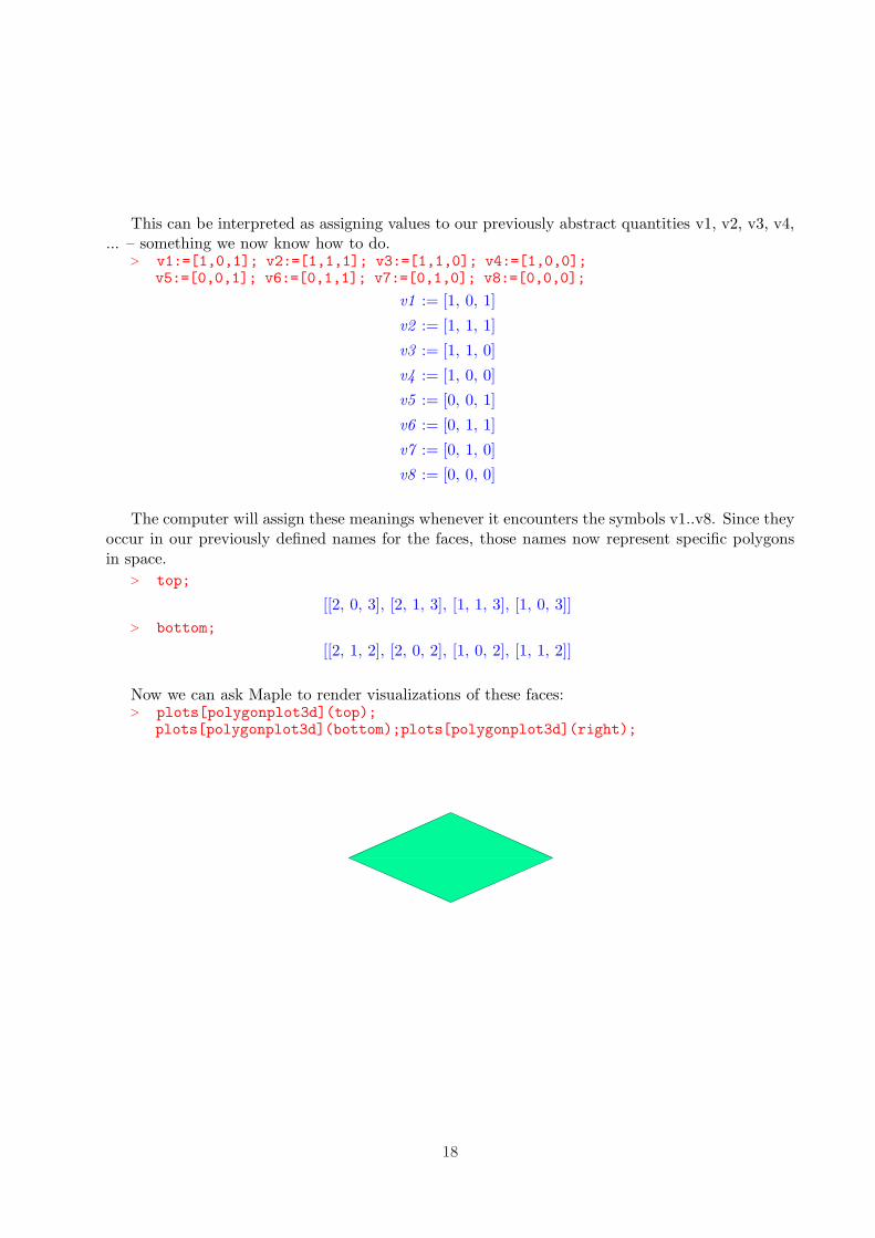
This can be interpreted as assigning values to our previously abstract quantities v1, v2, v3, v4,... – something we now know how to do.

> v1:=[1,0,1]; v2:=[1,1,1]; v3:=[1,1,0]; v4:=[1,0,0];v5:=[0,0,1]; v6:=[0,1,1]; v7:=[0,1,0]; v8:=[0,0,0];

v1 := [1, 0, 1]

v2 := [1, 1, 1]

v3 := [1, 1, 0]

v4 := [1, 0, 0]

v5 := [0, 0, 1]

v6 := [0, 1, 1]

v7 := [0, 1, 0]

v8 := [0, 0, 0]

The computer will assign these meanings whenever it encounters the symbols v1..v8. Since theyoccur in our previously defined names for the faces, those names now represent specific polygonsin space.

> top;

[[2, 0, 3], [2, 1, 3], [1, 1, 3], [1, 0, 3]]

> bottom;

[[2, 1, 2], [2, 0, 2], [1, 0, 2], [1, 1, 2]]

Now we can ask Maple to render visualizations of these faces:> plots[polygonplot3d](top);

plots[polygonplot3d](bottom);plots[polygonplot3d](right);

18

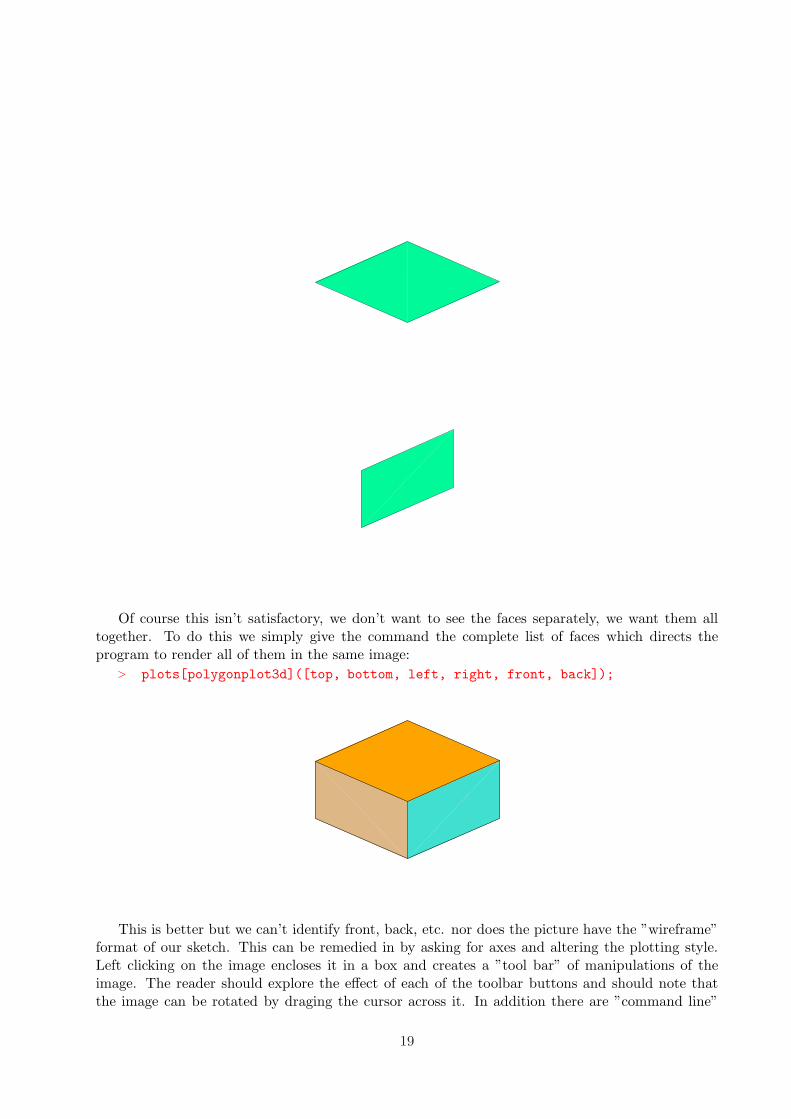
Of course this isn’t satisfactory, we don’t want to see the faces separately, we want them alltogether. To do this we simply give the command the complete list of faces which directs theprogram to render all of them in the same image:

> plots[polygonplot3d]([top, bottom, left, right, front, back]);

This is better but we can’t identify front, back, etc. nor does the picture have the ”wireframe”format of our sketch. This can be remedied in by asking for axes and altering the plotting style.Left clicking on the image encloses it in a box and creates a ”tool bar” of manipulations of theimage. The reader should explore the effect of each of the toolbar buttons and should note thatthe image can be rotated by draging the cursor across it. In addition there are ”command line”

19

options corresponding to each of the buttons on the tool bar. We will now explore several ofthem: style, scaling, and color which will be of immediate use. Each of these is an option for theplots[polygonplot3d] command. The way to learn about a command and its options is through thehelp system. As noted earlier this can be invoked in a number of ways. When we know exactly whatwe are looking for the command line approach is the most efficient:

> ?plots[polygonplot3d];

Note that the ”help” page this takes us to describes the command and refers us to other helpsheets for further information. We are interested in the options which we are told can be reachedby the command ?plot3d[options]; or by clicking on that hyperlink at the bottom of the sheet.In either case we reach a page which lists a large number of options. Our main objective at thispoint is to know that the page exists and how to reach it. A few examples of the use of some ofthe options generally suffices to give us enough information to work out for ourselves how othersare used. Note that the primary

> plots[polygonplot3d]

help sheet contains some examples. These can be copied and pasted into our work session andexecuted to see what they do. For now we will apply some of these options to our example. Firstlets take advantage of our ability to assign short names:

> box:=[top, bottom, right, left, front, back];

box := [[[2, 0, 3], [2, 1, 3], [1, 1, 3], [1, 0, 3]], [[2, 1, 2], [2, 0, 2], [1, 0, 2], [1, 1, 2]],

[[2, 1, 2], [2, 1, 3], [1, 1, 3], [1, 1, 2]], [[2, 0, 2], [1, 0, 2], [1, 0, 3], [2, 0, 3]],

[[2, 0, 3], [2, 1, 3], [2, 1, 2], [2, 0, 2]], [[1, 0, 3], [1, 1, 3], [1, 1, 2], [1, 0, 2]]]

Now we can simply have the computer draw ”box” - but we want to do this with some of theoptions. The first changes the plotting style from the default ”hidden line” to the ”wireframe”format indicated in our rough sketch.

> plots[polygonplot3d](box, style=wireframe);

We can color the edges of the frame as we wish. The response to ?plot3d[options];refers us

to plot[color]> ?plot3d[options]

> ?plot[color]

20

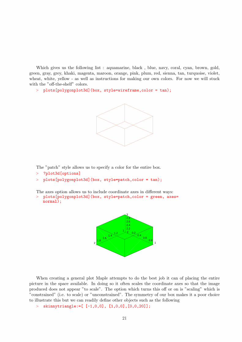
Which gives us the following list : aquamarine, black , blue, navy, coral, cyan, brown, gold,green, gray, grey, khaki, magenta, maroon, orange, pink, plum, red, sienna, tan, turquoise, violet,wheat, white, yellow - as well as instructions for making our own colors. For now we will stuckwith the ”off-the-shelf” colors.

> plots[polygonplot3d](box, style=wireframe,color = tan);

The ”patch” style allows us to specify a color for the entire box.

> ?plot3d[options]

> plots[polygonplot3d](box, style=patch,color = tan);

The axes option allows us to include coordinate axes in different ways:> plots[polygonplot3d](box, style=patch,color = green, axes=

normal);

22.22.42.62.83

0.20.4

0.60.8

1

11.2

1.41.6

1.82

When creating a general plot Maple attempts to do the best job it can of placing the entirepicture in the space available. In doing so it often scales the coordinate axes so that the imageproduced does not appear ”to scale”. The option which turns this off or on is ”scaling” which is”constrained” (i.e. to scale) or ”unconstrained”. The symmetry of our box makes it a poor choiceto illustrate this but we can readily define other objects such as the following

> skinnytriangle:=[ [-1,0,0], [1,0,0],[0,0,20]];

21

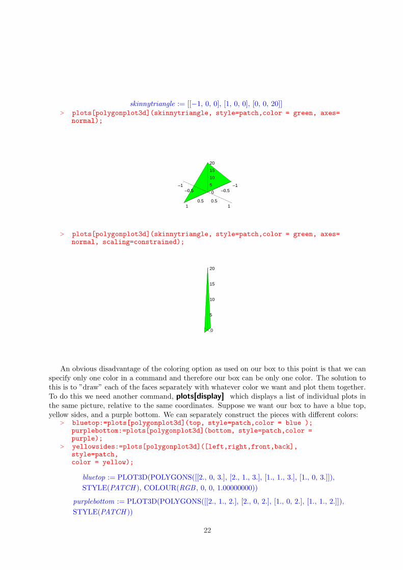
skinnytriangle := [[−1, 0, 0], [1, 0, 0], [0, 0, 20]]> plots[polygonplot3d](skinnytriangle, style=patch,color = green, axes=

normal);

0

5

10

15

20

–1–0.5

0.51

–1–0.5

0.51

> plots[polygonplot3d](skinnytriangle, style=patch,color = green, axes=normal, scaling=constrained);

0

5

10

15

20

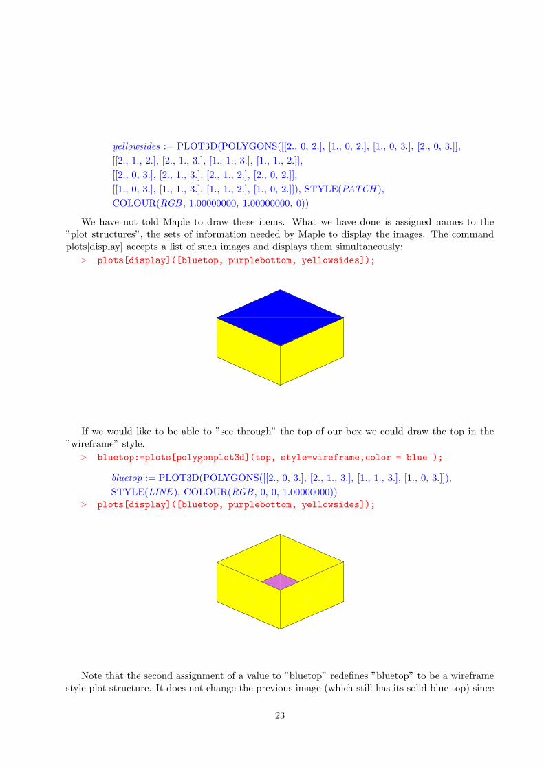
An obvious disadvantage of the coloring option as used on our box to this point is that we canspecify only one color in a command and therefore our box can be only one color. The solution tothis is to ”draw” each of the faces separately with whatever color we want and plot them together.To do this we need another command, plots[display] which displays a list of individual plots inthe same picture, relative to the same coordinates. Suppose we want our box to have a blue top,yellow sides, and a purple bottom. We can separately construct the pieces with different colors:

> bluetop:=plots[polygonplot3d](top, style=patch,color = blue );purplebottom:=plots[polygonplot3d](bottom, style=patch,color =purple);

> yellowsides:=plots[polygonplot3d]([left,right,front,back],style=patch,color = yellow);

bluetop := PLOT3D(POLYGONS([[2., 0, 3.], [2., 1., 3.], [1., 1., 3.], [1., 0, 3.]]),

STYLE(PATCH ), COLOUR(RGB , 0, 0, 1.00000000))

purplebottom := PLOT3D(POLYGONS([[2., 1., 2.], [2., 0, 2.], [1., 0, 2.], [1., 1., 2.]]),

STYLE(PATCH ))

22

yellowsides := PLOT3D(POLYGONS([[2., 0, 2.], [1., 0, 2.], [1., 0, 3.], [2., 0, 3.]],

[[2., 1., 2.], [2., 1., 3.], [1., 1., 3.], [1., 1., 2.]],

[[2., 0, 3.], [2., 1., 3.], [2., 1., 2.], [2., 0, 2.]],

[[1., 0, 3.], [1., 1., 3.], [1., 1., 2.], [1., 0, 2.]]), STYLE(PATCH ),

COLOUR(RGB , 1.00000000, 1.00000000, 0))

We have not told Maple to draw these items. What we have done is assigned names to the”plot structures”, the sets of information needed by Maple to display the images. The commandplots[display] accepts a list of such images and displays them simultaneously:

> plots[display]([bluetop, purplebottom, yellowsides]);

If we would like to be able to ”see through” the top of our box we could draw the top in the”wireframe” style.

> bluetop:=plots[polygonplot3d](top, style=wireframe,color = blue );

bluetop := PLOT3D(POLYGONS([[2., 0, 3.], [2., 1., 3.], [1., 1., 3.], [1., 0, 3.]]),

STYLE(LINE), COLOUR(RGB , 0, 0, 1.00000000))> plots[display]([bluetop, purplebottom, yellowsides]);

Note that the second assignment of a value to ”bluetop” redefines ”bluetop” to be a wireframestyle plot structure. It does not change the previous image (which still has its solid blue top) since

23

that is an image computed from the previous meaning. However if we now go back and re-evaluatethe command which produced that image the computation will be done with the current meaningof ”bluetop” and the resulting picture will be identical to the one immediately above.

Exercise (drawing colored cubes): Have Maple draw a cube on which each face hasa different color. Have it draw a cube on which each pair of opposite faces have thesame color but no two faces which share an edge have the same color.

We have seen that we can make new boxes from old ones by ”repainting” the faces of a singlebox or making some of the faces transparent. These ”new” boxes will, however, occupy exactly thesame position in space as the original. Suppose we want to ”stack” a copy of the original box ontop of it, or create a duplicate some distance away. This is extremely easy to do because of thegeneral nature of our approach. Our original sketch could have any box at all - it didn’t become aspecific box until we assigned values to the vertices v1..v8. Thus if we simply go back and assigndifferent values to the v1..v8 and execute all of the commands which followed we will duplicateeverthing we have done for a new box which can then be displayed along side the old one. Howeverat the outset of an investigation it is usually not a good idea to go back and change commandswhich we have working the way we want. It is MUCH better to copy the working commands thatwe want into the same or another worksheet and modify the copies. That way when somethingdoesn’t work we have a definite point at which to start ”debugging”. We will use the option ofcopying the commands we want into a new worksheet within the same Maple session.

2.3 Introductory Exercises: Drawing in the Plane

The following exercise set is a brief, ”get started” introduction to Maple. Follow the instructionsin order.

1. Open a new Maple worksheet by clicking on ”new” in the ”file menu”. Practice ”toggeling”between this and the new worksheet by selecting the appropriate worksheet in the ”Window” menu.Save the new worksheet using the ”Save As” option at the ”File” menu with an appropriate namesuch as ”EX CH1”.

*2. ”Select” this (entire) exercise set with the mouse and copy and paste it into the new work-

sheet.

ch1drawit3. Use ”Paint” or a similar program to draw a figure like the one above. Label the upper right

vertex ”V2” and the upper left ”V3”. Label the other edges ”left” and ”bottom” as appropriate.

PASTE THE DIAGRAM IN THE SPACE ABOVE

*4. Working in the new worksheet, break this exercise into distinct paragraphs (execution groups)

by placing the cursor at each asterisk to the left and pressing ”F3”. This can also be done at atthe ”Edit” menu at ”split or join” execution group.

24

*5. Delete each of the asterisks.*6. Open two command lines (execution groups) immediately below the each of your newly

created cells by use of the CONTROL J or at the ”Insert” Menu or by use of the large ”>” (greaterthan sign) on the toolbar. That is, place the cursor in the cell and then press CONTROL J or usethe menu or toolbar (twice). The result should be that each of the cells you created is followed bytwo new cells (execution groups) containing only a ”>” prompt .

*7. Follow each of the following instructions by entering the requested command on the first of

the command lines you opened. Commands for ”arithmetic”: Addition, multiplication, division,exponents, parenthesis, etc. follow the familiar syntax used with most calculators. For instanceone would enter 3*(5+3ˆ12)ˆ(2ˆ(11)); in order to calculate 3 (5 + 312)(2

11) .8. Add the numbers 1,3,17,-21,35,12*9. Multiply the numbers 1,3,17,-21,35,12* The ”ifactor” command allows you to factor integers, e.g ifactor(24); should return the

prime factorization of 24.*10. factor your social security number; factor your birth year.*11. Calculate 2(2j) + 1 and factor 2(2j) + 1 for j = 0,1,2,3,4,5,6,7. Do so by entering both

commands on the same command line below (each with its own semicolon) and subsequently bymodifying the commands, changing the ”j” to the next integer. (Until the turn of the century itwas thought that all such numbers were prime.)

*Maple will add, subtract, and multiply polynomial expressions. Typically a line like (x+y)*(x-

y); will return the ”unexpanded” version. The ”expand” command tells the computer to actuallymultiply out a polynomial expression in any number of variables, e.g. expand(x*(a+b)); andexpand((a+b)ˆ2); will produce just what one would expect. One can do things like assign a nameto an expression like joe:=expand((a+b)ˆ2); . The command ”factor” does for polynomialswhat ”ifactor” does for integers. Thus following the previous command one could factor(joe);

12. Have the computer do the polynomial multiplication (1-3*x+5*xˆ3)*(23-19*x+12*xˆ2);.

*13. Have the computer ”multiply out” (a + b)99. *14. Tell the computer to assign the value ”kate” to the result of expanding (2x + 3)50 out

”completely”.*15. Have the comuter to factor ”kate”.*16. Release 4 of Maple will ”add” lists (earlier versions will not) and multiply a number times

a list 2*[a,4]; returns [2a,8]) . If you have Release 4 or higher , tell Maple to add the lists [1,2,3],[4,5,6], and 7 times [a,b,c].

*

25

Maple knows all of the functions found on a graphics calculator and many more. The com-mand plot(sin(3*x),x=-2*Pi..2*Pi); will plot sin(3*x); from −2π to 2π. The commandplot({sin(3*x),sin(2*x), sin(x)} ,x=-2*Pi..2*Pi); will calculate the three functions sin(3x),sin(2x) and sin(x) at the same time.

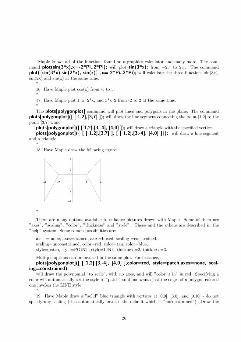
*16. Have Maple plot cos(x) from -5 to 3.*17. Have Maple plot 1, x, 2*x, and 3*xˆ2 from -2 to 2 at the same time.*The plots[polygonplot] command will plot lines and polygons in the plane. The command

plots[polygonplot]([ [ 1,2],[3,7] ]); will draw the line segment connecting the point [1,2] to thepoint [3,7] while

plots[polygonplot]([ [ 1,2],[3,-4], [4,0] ]); will draw a triangle with the specified vertices.plots[polygonplot]({ [ [ 1,2],[3,7] ], [ [ 1,2],[3,-4], [4,0] ]}); will draw a line segment

and a triangle.*18. Have Maple draw the following figure:

–4

–2

2

4

–4 –2 2 4

*

There are many options available to enhance pictures drawn with Maple. Some of them are”axes”, ”scaling”, ”color”, ”thickness” and ”style”. These and the others are described in the”help” system. Some comon possibilities are:

axes = none, axes=framed, axes=boxed, scaling =constrained,scaling=unconstrained, color=red, color=tan, color=blue,style=patch, style=POINT, style=LINE, thickness=2, thickness=3.

Multiple options can be invoked in the same plot. For instance,plots[polygonplot]([ [ 1,2],[3,-4], [4,0] ],color=red, style=patch,axes=none, scal-

ing=constrained);will draw the polynomial ”to scale”, with no axes, and will ”color it in” in red. Specifying a

color will automatically set the style to ”patch” so if one wants just the edges of a polygon coloredone invokes the LINE style.

*19. Have Maple draw a ”solid” blue triangle with vertices at [0,0], [3,0], and [0,10] - do not

specify any scaling (this automatically invokes the default which is ”unconstrained”). Draw the

26

same triangle ”to scale” with ”framed” axes. Draw the same triangle with no axes, do not fill itin, unconstrained, with the edges as ”thick” (thickness=3) red lines.

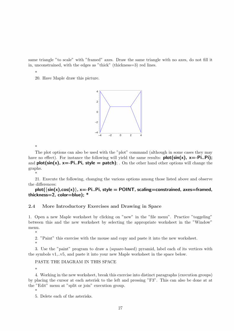
*20. Have Maple draw this picture.

–4

–2

0

2

4

–4 –2 0 2 4

*The plot options can also be used with the ”plot” command (although in some cases they may

have no effect). For instance the following will yield the same results: plot(sin(x), x=-Pi..Pi);and plot(sin(x), x=-Pi..Pi, style = patch); . On the other hand other options will change thegraphs.

*21. Execute the following, changing the varions options among those listed above and observe

the differences:plot({sin(x),cos(x)}, x=-Pi..Pi, style = POINT, scaling=constrained, axes=framed,

thickness=2, color=blue); *

2.4 More Introductory Exercises and Drawing in Space

1. Open a new Maple worksheet by clicking on ”new” in the ”file menu”. Practice ”toggeling”between this and the new worksheet by selecting the appropriate worksheet in the ”Window”menu.

*2. ”Paint” this exercise with the mouse and copy and paste it into the new worksheet.*3. Use the ”paint” program to draw a (square-based) pyramid, label each of its vertices with

the symbols v1,..v5, and paste it into your new Maple worksheet in the space below.

PASTE THE DIAGRAM IN THIS SPACE

*4. Working in the new worksheet, break this exercise into distinct paragraphs (execution groups)

by placing the cursor at each asterisk to the left and pressing ”F3”. This can also be done at atthe ”Edit” menu at ”split or join” execution group.

*5. Delete each of the asterisks.

27

*Open two command lines (execution groups) immediately below the each of your newly created

cells by use of the CONTROL J or at the ”Insert” Menu or by use of the large ”>” (greater thansign) on the toolbar. That is, place the cursor in the cell and then press CONTROL J or use themenu or toolbar (twice). The result should be that each of the cells you created is followed by twonew cells (execution groups) containing only a ”>” prompt .

Follow each of the following instructions by entering the requested command on the first of thecommand lines you opened.

Maple does arithmetic with integers (whole numbers: no decimal point) or fractions whosenumerator and deniminator are integers with no round off. If a single number in such a calculationhas a decimal (i.e. is a floating point number) then Maple carries the number of decimal digitsspecificd by the variable Digits . The default value of digits is 10. The user can change the valueof Digits by assigning a (positive integer) value to it.

6. Have Maple calculate 2ˆ100 and 100!*7. The Maple command ”sqrt” can be used to calculate square roots, To calculate the square

root of 19 use sqrt(19); Note the difference between sqrt(19); and sqrt(19.0);Have Maple display the first thousand digits of the square root of 2. Start with the command

Digits:=1000; When done be sure to reset the digits to 10.*8. Sometimes Maple’s accuracy obscures what we really want to know. For instance, is the

fraction 1399

12397 greater than 1 or less than 1? Enter joe:=13ˆ99/123ˆ97; and see if you can tell.

In such cases it is convenient to convert such experssions to floating point (decimal) approximationsfrom which we can readily answer such questions. The Maple command evalf (evaluate floatingpoint) does this. Try evalf(joe);

9. Maple stores 10000 digits of Pi but if you ask it to return Pi by entering the command Pi;you will just get a symbol. Use ”Digits” and ”evalf” to have Maple print out 5000 digits of Pi.Note that Pi is what Maple thinks is the ration of the circumference of a circle to its diameter; pi issimply another symbol with no independent interpretation. Note the difference between evalf(Pi);and evalf(pi);

*

10. We have seen that Maple can plot functions of one variable with plot . It can plot functionsof two variables with plot3d . To plot ”sin(xˆ2-yˆ2)” for x between -2 and 3 and y between -1 and2.5 use the command plot3d(sin(xˆ2-yˆ2),x=-1..3,y=-1..2.5);

*

The plots package contains many interesting three dimensional plotting tools. Among themost useful is plots[polygonplot3d], the analog of plots[polygonplot] in two dimensions. One mustkeep in mind that plots[polygonplot] expects lists of points in the plane while plots[polygonplot3d]expects lists of points in space. plots[polygonplot3d] will plot lines and polygons in the plane. Thecommand plots[polygonplot3d]([ [ 1,2,0],[3,7,0] ]); will draw the line segment connecting thepoint [1,2,0] to the point [3,7,0] while

plots[polygonplot3d]([ [ 1,2,0], [3,-4,0], [4,0,0] ]); will draw a triangle with the specified

28

vertices.plots[polygonplot3d]({ [ [ 1,2,0],[3,7,0] ], [ [ 1,2,0],[3,-4,0], [4,0,0] ]}); will draw a

line segment and a triangle.

> plots[polygonplot3d]({[[0,0,1],[1,0,1],[1,1,1],[0,1,1]],[[0,0,-1],[1,0,-1],[1,0,-1],[1,1,-1],[0,1,-1]],[[1/2,1/2,3],[1/2,1/2,-3]]},thickness=3,color=blue, style=patch, axes=boxed);

00.2

0.40.6

0.81

00.2

0.40.6

0.81

–3–2–10123

11. Make changes in the options invoked and observe the changes. Note that you can rotatethree dimensional plots by ”clicking” on them with the mouse, holding the mouse button down and”dragging” the reference box (which represents the figure) around. Double clicking on the figureor selecting ”R” for (redraw) at the tool bar will draw the rotated figure.

Exercise (drawing colored cubes): Have Maple draw a cube on which each face hasa different color. Have it draw a cube on which each pair of opposite faces have thesame color but no two faces which share an edge have the same color.

29

3 Translating Geometric Objects

3.1 Duplicating and moving cubes

In this chapter we will see how to draw cubes and shift them around. Of course there are variousways to do this. We could use words from the plottools package to draw and move the cube,but here we will use a more direct approach. We will begin to make use of the colon colon ”:”terminator for commands to suppress unwanted output. Note that the colon can always be replacedby a semicolon and the command re-executed if we need to look at the output.

A cube has eight vertices, and we can name the six sides of the cube using those vertices.> front:=[v1,v2,v3,v4]:back:=[v5,v6,v7,v8]:left:=[v4,v8,v5,v1]:right:=[

v3,v2,v6,v7]:bottom:=[v3,v4,v8,v7]: top:=[v1,v2,v6,v5]:

For starters, give specific value for these vertices.> v1:=[1,0,1]: v2:=[1,1,1]: v3:=[1,1,0]: v4:=[1,0,0]:

v5:=[0,0,1]: v6:=[0,1,1]: v7:=[0,1,0]: v8:=[0,0,0]:

Now, the cube or box consists of the 6 sides. We can draw the box using polygonplot3d.> box:=[top, bottom, right, left, front, back]:

> plots[polygonplot3d](box);

The sides can be colored individually if we choose to do that. For example we might want thetop to be blue, the bottom magenta, and the sides yellow.

> bluetop:=plots[polygonplot3d](top, style=patch,color = blue ):

> purplebottom:=plots[polygonplot3d](bottom, style=patch,color = magenta):yellowsides:=plots[polygonplot3d]([left,right,front,back],style=patch,color = yellow):

> plots[display]([bluetop, purplebottom, yellowsides]);

30

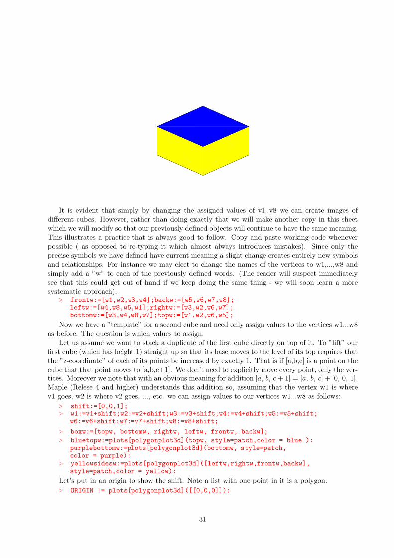
It is evident that simply by changing the assigned values of v1..v8 we can create images ofdifferent cubes. However, rather than doing exactly that we will make another copy in this sheetwhich we will modify so that our previously defined objects will continue to have the same meaning.This illustrates a practice that is always good to follow. Copy and paste working code wheneverpossible ( as opposed to re-typing it which almost always introduces mistakes). Since only theprecise symbols we have defined have current meaning a slight change creates entirely new symbolsand relationships. For instance we may elect to change the names of the vertices to w1,...,w8 andsimply add a ”w” to each of the previously defined words. (The reader will suspect immediatelysee that this could get out of hand if we keep doing the same thing - we will soon learn a moresystematic approach).

> frontw:=[w1,w2,w3,w4];backw:=[w5,w6,w7,w8];leftw:=[w4,w8,w5,w1];rightw:=[w3,w2,w6,w7];bottomw:=[w3,w4,w8,w7];topw:=[w1,w2,w6,w5];

Now we have a ”template” for a second cube and need only assign values to the vertices w1...w8as before. The question is which values to assign.

Let us assume we want to stack a duplicate of the first cube directly on top of it. To ”lift” ourfirst cube (which has height 1) straight up so that its base moves to the level of its top requires thatthe ”z-coordinate” of each of its points be increased by exactly 1. That is if [a,b,c] is a point on thecube that that point moves to [a,b,c+1]. We don’t need to explicitly move every point, only the ver-tices. Moreover we note that with an obvious meaning for addition [a, b, c + 1] = [a, b, c] + [0, 0, 1].Maple (Relese 4 and higher) understands this addition so, assuming that the vertex w1 is wherev1 goes, w2 is where v2 goes, ..., etc. we can assign values to our vertices w1...w8 as follows:

> shift:=[0,0,1];> w1:=v1+shift;w2:=v2+shift;w3:=v3+shift;w4:=v4+shift;w5:=v5+shift;

w6:=v6+shift;w7:=v7+shift;w8:=v8+shift;

> boxw:=[topw, bottomw, rightw, leftw, frontw, backw];> bluetopw:=plots[polygonplot3d](topw, style=patch,color = blue ):

purplebottomw:=plots[polygonplot3d](bottomw, style=patch,color = purple):

> yellowsidesw:=plots[polygonplot3d]([leftw,rightw,frontw,backw],style=patch,color = yellow):

Let’s put in an origin to show the shift. Note a list with one point in it is a polygon.> ORIGIN := plots[polygonplot3d]([[0,0,0]]):

31

> plots[display]([ ORIGIN,bluetopw, purplebottomw, yellowsidesw],axes=normal);

Reference to the axes verifies that our new cube is indeed a copy of the old one shifted upexactly one uint. The question now is how to display them at the same time. The answer is thatwe do exactly what we did before.

> plots[display]([ plots[display]([bluetop, purplebottom,yellowsides]),plots[display]([bluetopw, purplebottomw, yellowsidesw], axes=normal)]);

The command above obviously stacked our cubes although we do see here the need to tellMaple not to scale the image if we want the cubes to appear as such. That is easily remedied.More important is to understand how what the above command did and how to abbreviate it.The plots[display] command takes in lists of plot structures and outputs a plot structure. Each ofour cubes is such an output and . Thus this command is of the form plots[display]([plotstructure1,plotstructure2], axes=normal). We can make the assignments:

> cube1:=plots[display]([bluetop, purplebottom, yellowsides]):

> cube2:=plots[display]([bluetopw, purplebottomw, yellowsidesw]):

Then we can express the command which generated the ”stacked” cubes in the form

> plots[display]([cube1, cube2], axes=normal, scaling=constrained);

Note that we have added the option scaling=constrained to give our pictures the proper scale.

There is no reason to for both cubes the same color or style, we can give the faces of cube2 anycolor or style we want. What if we want a cube3? The obvious ways to produce a cube3 are repeatwhat we did to get cube2 or even to take the tack we avoided then and simply modify our previouscode to produce a cube3. Keeping in mind that once we have produced cube2 if we then redefinethe vertices w1..w8 we can produce a separate cube3, retaining the picture of our ”original” cube2but not cube2 itself. We could do the same thing to get a cube4, cube5, etc. If all we want are thepictures this will work but there are problems. For instance, suppose we wanted 100 cubes madethem all yellow and then decided that they should be red. We would have to repeat all of thesesteps ”by hand”. Fortunately, Maple provides tools to automate this type of manufacturing process.What we need to do is build a new Maple word which takes the original cube and produces a set of”stacked” copies (or a picture of such a set) assembled according to our instructions. We will takeup this process in the next chapter but first we want to actually build a few new cubes and assemblethem in order to gain a firm grasp of exactly what process we want to automate. This will be aprocess we will repeat many times in this study. First let us block out what we did to get cube1.

3.2 The steps in building a cube

1. Define the original, abstract cube ”box” as a list of faces where each face was itself a list ofvertices v1..v8.

2. Assign specific values to the vertices v1..v8. Doing so automatically caused Maple to interpretthe abstract cube, box, as the specific cube with the vertices assigned to v1..v8.

3. Execute a command cube1:=plots[polygonplot3d](box, options) which produced a plot struc-ture representing the current ”value” of ”box”

32

Now let us extend these steps to the process which produced cube2 - but this time re-assigningthe values of the v1..v8 rather than introducing the new vertices.

4. Assign a specific value to the word ”shift” (note there is nothing special about the word”shift”, ”yzkotqp” would work just as well but would be less intuitive and perhaps harder toremember).

5. Assign new values to v1..v8 by the assignment commands v1:=v1+shift; v2:=v2+shift; ...,which say ”the new value of v1 is the current value of v1 plus shift, etc.

6. Execute the command cube2:=plots[polygonplot3d](box, options)

7. go to step 4.

3.3 Building a TEE

Lets create an assemblage of cubes in the shape of a ”T” as in the following sketch.

ch2teeAlthough we don’t really need to we will repeat the initial steps. This time we will use a

different notation for the pictures of the faces which doesn’t designate theircolors so that we may feel free to vary these as we wish. In addition, we introduce the ”shift”

immediately and simply let it be [0,0,0] to start.

> v1:=[1,0,1]: v2:=[1,1,1]: v3:=[1,1,0]: v4:=[1,0,0]:v5:=[0,0,1]: v6:=[0,1,1]: v7:=[0,1,0]: v8:=[0,0,0]:

> shift:=[0,0,0]:> v1:=v1+shift: v2:=v2+shift: v3:= v3+shift: v4:=v4+shift:

v5:=v5+shift: v6:=v6+shift: v7:=v7+shift: v8:=v8+shift:front:=[v1,v2,v3,v4]:back:=[v5,v6,v7,v8]:left:=[v4,v8,v5,v1]:right:=[v3,v2,v6,v7]:bottom:=[v3,v4,v8,v7]:top:=[v1,v2,v6,v5]:

> toppic:=plots[polygonplot3d](top, style=patch,color = blue ):bottompic:=plots[polygonplot3d](bottom, style=patch,color = magenta):sidespic:=plots[polygonplot3d]([left,right,front,back],style=patch,color = yellow):

> cube1:=plots[display]([ toppic, bottompic, sidespic]):

Now we have cube1, all we need do now is reset the shift and repeat the second group ofcommands, changing only the name of the result to ”cube2”.

> v1:=[1,0,1]: v2:=[1,1,1]: v3:=[1,1,0]: v4:=[1,0,0]:v5:=[0,0,1]: v6:=[0,1,1]: v7:=[0,1,0]: v8:=[0,0,0]:

> shift:=[0,0,1]:

> v1:=v1+shift: v2:=v2+shift: v3:= v3+shift: v4:=v4+shift: v5:=v5+shift: v6:=v6+shift:

v7:=v7+shift: v8:=v8+shift: front:=[v1,v2,v3,v4]:back:=[v5,v6,v7,v8]:left:=[v4,v8,v5,v1]:

right:=[v3,v2,v6,v7]:bottom:=[v3,v4,v8,v7]:top:=[v1,v2,v6,v5]:

33

> toppic:=plots[polygonplot3d](top, style=patch,color = blue ):bottompic:=plots[polygonplot3d](bottom, style=patch,color = purple):sidespic:=plots[polygonplot3d]([left,right,front,back], style=patch,color = yellow):


Now cube3 results from a shift of two units straight up> v1:=[1,0,1]: v2:=[1,1,1]: v3:=[1,1,0]: v4:=[1,0,0]:

v5:=[0,0,1]: v6:=[0,1,1]: v7:=[0,1,0]: v8:=[0,0,0]:

> shift:=[0,0,2]:

> v1:=v1+shift: v2:=v2+shift: v3:= v3+shift: v4:=v4+shift:v5:=v5+shift: v6:=v6+shift: v7:=v7+shift: v8:=v8+shift:front:=[v1,v2,v3,v4]:back:=[v5,v6,v7,v8]:left:=[v4,v8,v5,v1]:right:=[v3,v2,v6,v7]:bottom:=[v3,v4,v8,v7]:top:=[v1,v2,v6,v5]:

> toppic:=plots[polygonplot3d](top, style=patch,color = blue ):bottompic:=plots[polygonplot3d](bottom, style=patch,color = purple):sidespic:=plots[polygonplot3d]([left,right,front,back], style=patch,color = yellow):


Cube4 is two up and one to the ”right”> v1:=[1,0,1]: v2:=[1,1,1]: v3:=[1,1,0]: v4:=[1,0,0]:

v5:=[0,0,1]: v6:=[0,1,1]: v7:=[0,1,0]: v8:=[0,0,0]:

> shift:=[-1,0,2]:


> toppic:=plots[polygonplot3d](top, style=patch,color = blue ):bottompic:=plots[polygonplot3d](bottom, style=patch,color = magenta):sidespic:=plots[polygonplot3d]([left,right,front,back], style=patch,color = yellow):


And cube5 results from a shift of two up and one to the ”left”

> v1:=[1,0,1]: v2:=[1,1,1]: v3:=[1,1,0]: v4:=[1,0,0]:v5:=[0,0,1]: v6:=[0,1,1]: v7:=[0,1,0]: v8:=[0,0,0]:

> shift:=[1,0,2]:


> toppic:=plots[polygonplot3d](top, style=patch,color = blue ):bottompic:=plots[polygonplot3d](bottom, style=patch,color = magenta):sidespic:=plots[polygonplot3d]([left,right,front,back], style=patch,color = yellow):

34


We have not taken the time to change the colors on our various cubes but we could have, simplyby changing the options for each of them. Lets make our cubes into a list and display them

> cubes:=[cube1,cube2,cube3,cube4,cube5]:

Finally, we can display our cubes. Since its to be a ”T” we’ll call it ”Tee”. The followingcommand will then assign that plot structure to the symbol ”Tee”. It will not display it. On theother hand, Tee then becomes a Maple word whose value is that plot structure so when Maplereceives ”Tee” from the command line it will respond return ”Tee” in the manner it represents suchstructures - namely by plotting them.

Error, (in plot/color) invalid color specification: purple

Error, (in plot/color) invalid color specification: purple

> Tee:=plots[display](cubes, scaling=constrained):

> Tee;

Exercise: The ”T” generated previously is an example of a figure that can be madeby five identical cubes such that each of them share a face with at least one other.There is an ”L” figure which can be made with 4. Find all of the figures of this typewhich can be made using either three or four cubes and construct a Maple word foreach one which displays it. We regard two figures as the same if they are congruent inthe sense of geometry - that is if one could be moved and rotated in space to becomecoincident with the other. Include a careful explanation of why your list is complete.

3.4 Exercises: More Pictures in the Plane

Although we have concentrated on ”3d” graphics in the text one often wants to work with ”2d”versions of the same problems. Not only may the problem be inherently two dimensional butcomputer resources required for three dimensions may severely limit what we can do on a particularmachine. In this exercise we will discuss translating planar boxes.

0. If you have not read through and executed the main worksheet for this exercise go to thebeginning of this worksheet and execute the first few commands.

1. Copy this entire exercise set into a new worksheet and begin work in the new worksheet.

3.. Use ”Paint” or a similar program to draw a figure like this oneLabel the upper right vertex”V2” and the upper left ”V3”. Label the other edges ”left” and ”bottom” as appropriate

ch2diagr

PASTE YOUR DIAGRAM IN THIS AREA

4. Enter the commands top; right; left; bottom;

35

at the prompt. If Maple returns anything but these names then they already have assignedvalues - this will be the case if you have just executed the first few commands in the worksheet.Note that all worksheets open at any one time share a common set of variables. Thus (assumingexercise 1 was done) even though we are in a different worksheet, the value of ”top” from theoriginal is shared by this ”new” one.

We want to assign new values to these symbols for our ”plane” work. For instance we will want”bottom” to be the list ”[v0,v1]” and to represent the bottom edge of the figure we have drawn. Ifwe are careful in making these assignments then we will simply ”overwrite” the previous meaningsof the words with new assignments. However were we to forget to actually make the assignment for,say, ”left” then subsequent execution errors will occur which can be quite difficult to track down.In addition, when we change the value of ”top” in the new worksheet its ”new” value will be usedin subsequent calculations in other worksheets - but will not affect the current values from earliercalculations. That is, it doesn’t work like a spreadsheet, previous calculations are not automatically”updated”. In most cases the simplest thing to do is issue the command restart; restart; Thisresets all variables to their default value which is simply their name. That is what we will do. Issuethe command restart;

Now re-enter the commands top; right; left; bottom;

5. Assign the list ”[v0,v1]” to the name ”bottom” with the command bottom:=[v0,v1]; Sim-ilarly assign the appropriate lists to ”right”, ”left”, and ”bottom”. Assign the name ”box” to thelist [bottom, right, top, left]

6. The computer is unable graphically interpret quantities that are not completely described,A person can relate the list [v0,v1] to a general line segment but the computer needs to knowprecisely what v0 and v1 are in order to interpret it as a line segment. Issue the commandplots[polygonplot]([v0,v1]); then issue the command plots[polygonplot]([[0,0],[1,1]]);

7. Assign values [0,0] to v0, [1,0[ to v1, [1,1] to v2, and [0,1] to v3 and have Maple drawthe edges of the square with the command plots[polygonplot] plots[polygonplot] Draw thetop and left edges at the same time with plots[polygonplot]([top, left]); Draw the entire box withplots[polygonplot](box);

NOTE: If/when you subsequently re-define the values of v0,v1,v2,v3 if you do not also ”update”the interpretation of ”box” (for instance by re-issueing the defining command that defined ”box”)then the command plots[polygonplot](box); will draw the previously defined box.

8.Recall that there are many options available to enhance pictures drawn with Maple. Some ofthem are ”axes”, ”scaling”, ”color”, ”thickness” and ”style”. These and the others are describedin the ”help” system. Some comon possibilities are:

36

axes = none, axes = framed, axes = boxed, scaling = constrained , scaling = unconstrained,color = red, color = tan, color = blue, style = patch, style = POINT, style = LINE, thickness =2, thickness = 4

Multiple options can be invoked in the same plot. For instance ,plots[polygonplot]( box,color=green, style=patch,axes=none, thickness=4); will draw the box

with no axes, and will ”color it in” in green. Specifying a color will automatically set the style to”patch” so if one wants just the edges of a polygon colored one invokes the LINE style.

*

10. If P= [a,b] is a point in the plane and we want the point Q which is the result of shiftingP by 1 to the right and up 4 then Q=[a+1,b+4]. Similarly if we want Z which is the result ofshifting P by 3 to the left and down 7 then Z=[a -3,b-7]. We can write Q= P+[1,4] and Z =P+[-3,-7]. Beginning with release 4, Maple understands this ”list arithmetic” which allows us toinstruct Maple to ”shift” objects in the plane.

If v0,v1,v2,v3 are the vertices of a box which is shifted so that each point of the box move ”a”to the right and ”b” to the left then if we ”shift” be [a,b], the shifted box is [v0+shift,v1+shift,v2+shift,v3+shift]. If ”shift” is [0,0] then this is simply the original box.

We want to define a new ”abstract” box called ”sbox” (for ”shifted box) which contains the(currently undefined) quantity ”shift”. However if we do the ”obvious” something which mightnot be expected will happen if we have been doing the previous exercises in the current session.Execute the command sbox:=[v0+shift,v1+shift, v2+shift,v3+shift];

If you got the error message ”adding lists of different length” this was probably because v0...v3had meaning as lists of length 2 from the previous work while ”shift” is just a name with no suchmeaning. One way out of this is to use symbols other than v0,v1..,v3. Edit the previous commandto sbox:=[w0+shift,w1+shift, w2+shift,w3+shift]; If w0..etc had not been previously assigned somemeaning and ”shift” hasn’t acquired one then this will work fine. However it begs the question ofwhat to do if we subsequently need ”w0” for another purpose. What one needs to do is ”reset”v0,v1, etc (and possibly ”shift”) to their default values. In principle we could use the commandrestart but this would reset all variables in all worksheets in this session.

The commands v0:=’v0’; v1:=’v1’; v2:=’v2’; v3:=’v3’; shift:=’shift’; assign to each of thesevaraiables its own name, which is its default value. Once these are executed the definition of”sbox” will work fine.

11. With ”sbox” abstractly defined one can proceed as before to draw general quadralateralsin the plane by specifying (assigning) values for v0...v3 and ”shift”.

Assign v0,v1,v2,v3 the values [0,0], [1,0], [ 1,1], and [0,1], and ”shift” the value [2,3]. The usethe command

plots[polygonplot](sbox, color = green, style = patch, axes = normal);to draw the shifted box.

37

12. One can assign a name to a plot and subsequently display that plot by invoking its name.For instance joe:=plots[polygonplot](box,color=blue, style=LINE, thickness=4, axes=normal); willdisplay Maple’s internal description of the figure, In this case the internal description is very shortand interesting to view. In general it may run many, many pages and one does not want to see it.This is a case where the colon delimiter is very useful. Run joe:=plots[polygonplot](box,color=blue,style=LINE, thickness=4, axes=normal): then joe;

13. With the ability to make and ”store” different pictures we can collect different picturesand display them together, creating more complex images. For instance the following is simply acollection of images of squares made one at a time. Each is a shift of the basic ”unit box”, (v0=[0,0],v1=[1,0],v2=[1,1],v3=[0,1]), made by a sequence of commands of the form

shift:= [1,3]; sbox:=[v0+shift,v1+shift,v2+shift,v3+shift]; bx1:=plots[polygonplot]( sbox,color=green,style=patch,axes=norma l l

The command to display the members of a list a collection of plots images at the same timeis plots[display]. plots[display]. Thus for instance if, using the above command sequence onemakes images 4 images bx1, bx2, bx3, bx4t. The command to display them all at once would beplots[display([bx1,bx2,bx2,bx3,bx4]); Of course one could make a list bx:=[bx1,bx2,bx3,bx4]; andsimply do plots[display](bx);

Note that one can use different plot options in each image. One can also include options inplots[display]: plots[display](bx,scaling=constrained);

Have Maple draw this picture.

0

0.5

1

1.5

2

0 1 2 3 4

3.5 Exercises: Making 3d Alphabet Blocks Exercises: Making 3d AlphabetBlocks

Introduction: One often finds colored cubes as children’s toys and these often haveletters painted on them. Lets investigate the possibility of making a white cube witha blue ”K” on one face. The white cube is no problem, we’ve done that before. Weneed to make the ”K”. We know how to make polygons so we want a ”K” thats madeof them.

38

ch2kayThis one is made of the polygons A,B, and C. All we need to do is draw something like this on

a piece of graph paper, read off the coordinates of the vertices, make up each of the polygons andput them together.

> A:=[[1/10,0,1/10],[1/10,0,9/10],[3/10,0,9/10],[3/10,0,1/10]]:

> B:=[[3/10,0,4/10],[3/10,0,6/10],[6/10,0,9/10],[9/10,0,9/10]]:

> C:=[[4/10,0,5/10],[6/10,0,6/10],[9/10,0,1/10],[7/10,0,1/10]]:> K:=plots[polygonplot3d]([A,B,C],color=blue,style=patch):

K;

Now we need the cube. As before we retrieve our basic box construction. Then we will jam theK onto the cube and look. After looking, we see that the K is on the other side, so we insert anorientation=[-49,60] in order to position it initially (We obtained this orientation by experiment).

> v1:=[1,0,1]: v2:=[1,1,1]: v3:=[1,1,0]: v4:=[1,0,0]:v5:=[0,0,1]: v6:=[0,1,1]: v7:=[0,1,0]: v8:=[0,0,0]:

> box:=[top, bottom, right, left, front, back]:> front:=[v1,v2,v3,v4]:back:=[v5,v6,v7,v8]:left:=[v4,v8,v5,v1]:

right:=[v3,v2,v6,v7]:bottom:=[v3,v4,v8,v7]:top:=[v1,v2,v6,v5]:> whitecube:=plots[polygonplot3d](box, color=white,

style=patch,thickness=3):> Kcube:=plots[display]([K,whitecube],axes=boxed,orientation=[-49,60]):

Kcube;

00.2

0.40.6

0.81

0.20.4

0.60.8

10

0.2

0.4

0.6

0.8

1

39

There are two problems here. The first is a very sloppy ”K” which results from inaccuratereading of coordinates from a hastily drawn graph. This can be partially addressed by more carefulgraphing. The second problem is that some views show a two-toned ”K”. This is what happenswhen two patch-style pictures are in contact. The patch pictures are made of colored trianglesoccupying the same positions and the computer doesn’t know which onw we really want to see.The solution is to move them slightly apart. In this case its we might have the ”K” as being slightlyraised above the surface of the cube. That just means altering the definition of K. Note the smallchanges in the y-coordinate of the vertices in order to move the K off the surface.

> A:=[[1/10,-.01,1/10],[1/10,-.01,9/10],[3/10,-.01,9/10],[3/10,-.01,1/10]]:

> B:=[[3/10,-.01,4/10],[3/10,-.01,6/10],[6/10,-.01,9/10],[9/10,-.01,9/10]]:

> C:=[[4/10,-.01,5/10],[6/10,-.01,6/10],[9/10,-.01,1/10],[7/10,-.01,1/10]]:

> K:=plots[polygonplot3d]([A,B,C],color=blue,style=patch):> Kcube:=plots[display]([K,whitecube],orientation=[-50,75]):

Kcube;

EXERCISES:1. Improve the ”Kcube” by creating one with a better ”K” by more careful graphing.2. Change the ”Kcube” so that there is a ”K” on each face.3. Make a yellow block with one the letters A,B,C,D,E,F on each face.4. Give each of the letters in the previous problem a different color.5. Make the block in the previous problem appear to be made of a transparent material with

the colored letters painted on its faces. HINT: Wireframe6. Make a row of alphabet blocks that display your initials.7. Create a ”solid” ”K”

40

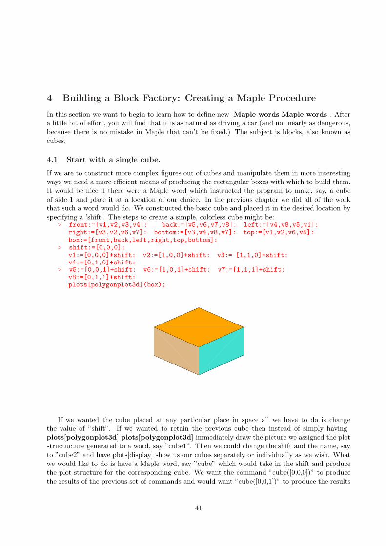
4 Building a Block Factory: Creating a Maple Procedure

In this section we want to begin to learn how to define new Maple words Maple words . Aftera little bit of effort, you will find that it is as natural as driving a car (and not nearly as dangerous,because there is no mistake in Maple that can’t be fixed.) The subject is blocks, also known ascubes.

4.1 Start with a single cube.

If we are to construct more complex figures out of cubes and manipulate them in more interestingways we need a more efficient means of producing the rectangular boxes with which to build them.It would be nice if there were a Maple word which instructed the program to make, say, a cubeof side 1 and place it at a location of our choice. In the previous chapter we did all of the workthat such a word would do. We constructed the basic cube and placed it in the desired location byspecifying a ’shift’. The steps to create a simple, colorless cube might be:

> front:=[v1,v2,v3,v4]: back:=[v5,v6,v7,v8]: left:=[v4,v8,v5,v1]:right:=[v3,v2,v6,v7]: bottom:=[v3,v4,v8,v7]: top:=[v1,v2,v6,v5]:box:=[front,back,left,right,top,bottom]:

> shift:=[0,0,0]:v1:=[0,0,0]+shift: v2:=[1,0,0]+shift: v3:= [1,1,0]+shift:v4:=[0,1,0]+shift:

> v5:=[0,0,1]+shift: v6:=[1,0,1]+shift: v7:=[1,1,1]+shift:v8:=[0,1,1]+shift:plots[polygonplot3d](box);

If we wanted the cube placed at any particular place in space all we have to do is changethe value of ”shift”. If we wanted to retain the previous cube then instead of simply havingplots[polygonplot3d] plots[polygonplot3d] immediately draw the picture we assigned the plotstructucture generated to a word, say ”cube1”. Then we could change the shift and the name, sayto ”cube2” and have plots[display] show us our cubes separately or individually as we wish. Whatwe would like to do is have a Maple word, say ”cube” which would take in the shift and producethe plot structure for the corresponding cube. We want the command ”cube([0,0,0])” to producethe results of the previous set of commands and would want ”cube([0,0,1])” to produce the results

41

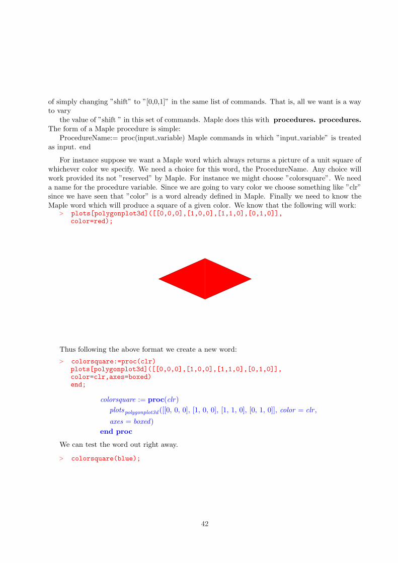
of simply changing ”shift” to ”[0,0,1]” in the same list of commands. That is, all we want is a wayto vary

the value of ”shift ” in this set of commands. Maple does this with procedures. procedures.The form of a Maple procedure is simple:

ProcedureName:= proc(input variable) Maple commands in which ”input variable” is treatedas input. end

For instance suppose we want a Maple word which always returns a picture of a unit square ofwhichever color we specify. We need a choice for this word, the ProcedureName. Any choice willwork provided its not ”reserved” by Maple. For instance we might choose ”colorsquare”. We needa name for the procedure variable. Since we are going to vary color we choose something like ”clr”since we have seen that ”color” is a word already defined in Maple. Finally we need to know theMaple word which will produce a square of a given color. We know that the following will work:

> plots[polygonplot3d]([[0,0,0],[1,0,0],[1,1,0],[0,1,0]],color=red);

Thus following the above format we create a new word:

> colorsquare:=proc(clr)plots[polygonplot3d]([[0,0,0],[1,0,0],[1,1,0],[0,1,0]],color=clr,axes=boxed)end;

colorsquare := proc(clr)

plotspolygonplot3d ([[0, 0, 0], [1, 0, 0], [1, 1, 0], [0, 1, 0]], color = clr ,

axes = boxed)

end proc

We can test the word out right away.

> colorsquare(blue);

42

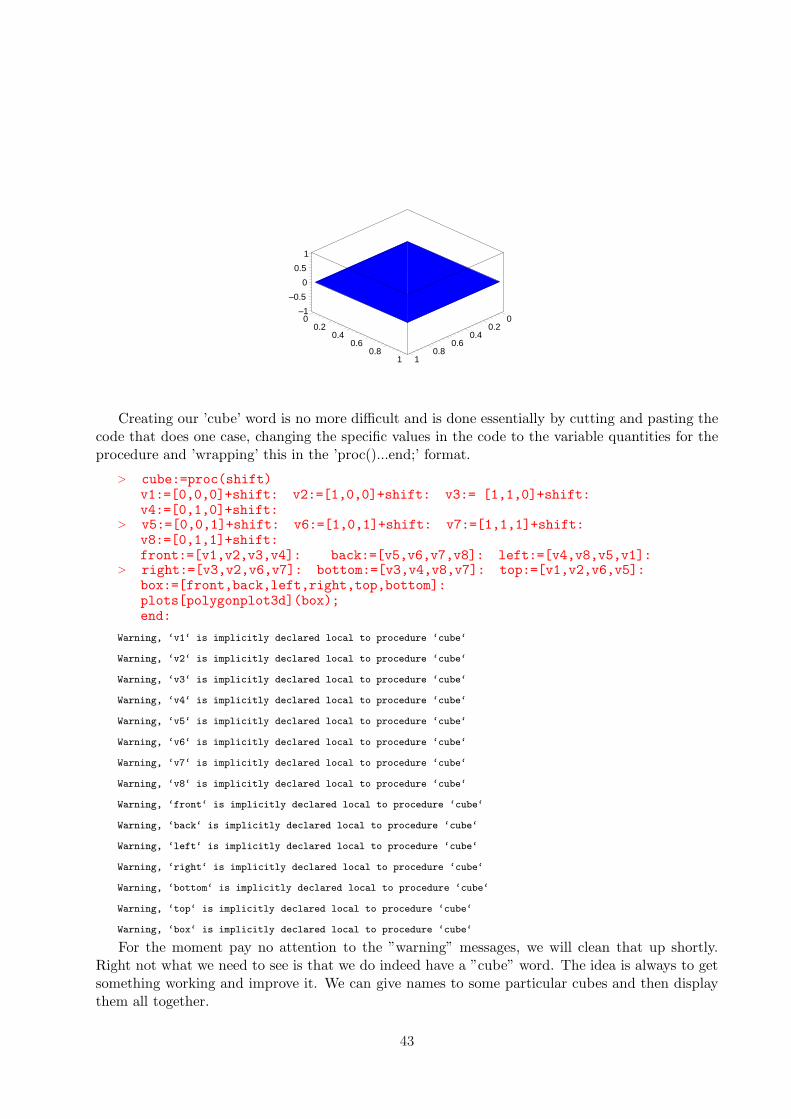
00.2

0.40.6

0.81

00.2

0.40.6

0.81

–1

–0.5

0

0.5

1

Creating our ’cube’ word is no more difficult and is done essentially by cutting and pasting thecode that does one case, changing the specific values in the code to the variable quantities for theprocedure and ’wrapping’ this in the ’proc()...end;’ format.

> cube:=proc(shift)v1:=[0,0,0]+shift: v2:=[1,0,0]+shift: v3:= [1,1,0]+shift:v4:=[0,1,0]+shift:

> v5:=[0,0,1]+shift: v6:=[1,0,1]+shift: v7:=[1,1,1]+shift:v8:=[0,1,1]+shift:front:=[v1,v2,v3,v4]: back:=[v5,v6,v7,v8]: left:=[v4,v8,v5,v1]:

> right:=[v3,v2,v6,v7]: bottom:=[v3,v4,v8,v7]: top:=[v1,v2,v6,v5]:box:=[front,back,left,right,top,bottom]:plots[polygonplot3d](box);end:

Warning, ‘v1‘ is implicitly declared local to procedure ‘cube‘








Warning, ‘front‘ is implicitly declared local to procedure ‘cube‘

Warning, ‘back‘ is implicitly declared local to procedure ‘cube‘

Warning, ‘left‘ is implicitly declared local to procedure ‘cube‘

Warning, ‘right‘ is implicitly declared local to procedure ‘cube‘

Warning, ‘bottom‘ is implicitly declared local to procedure ‘cube‘

Warning, ‘top‘ is implicitly declared local to procedure ‘cube‘

Warning, ‘box‘ is implicitly declared local to procedure ‘cube‘

For the moment pay no attention to the ”warning” messages, we will clean that up shortly.Right not what we need to see is that we do indeed have a ”cube” word. The idea is always to getsomething working and improve it. We can give names to some particular cubes and then displaythem all together.

43

> joe:=cube([1,2,4]):sam:=cube([1,0,1]):sally:=cube([1,1,1]):

> plots[display]([joe,sam,sally],color=red,scaling=constrained,axes=boxed);

11.5

2

00.5

11.5

22.5

3

1

2

3

4

5

When a word which is not a Maple or user-defined word is used within a Maple procedure itis allowed to have meaning only within the procedure. It is used only locally, hence the ”localvariable” designation. This allows words to be used within procedures that actually have anexternal meaning. This is very useful in the development of procedures. For instance, our objectivein developing ”cube” to no longer have to think about its details when we need a cube in the future.Suppose we were to use it in the future as part of a project in which we have also used the word”top” to mean the amount of fuel in a tank when it is full. Now having forgotten all about theinternal workings of ”cube” we issue the command ”cube([0,0,0])”. Note that within ”cube” thereis a command ”top:=[v1,v2,v6,v5]”. If ”top” in ”cube” were not restricted to have meaning onlywithin that procedure its invovation would have changed the ”top” we were thinking of from anumber to a four element list. This could cause all kinds of problems.

The default is that Maple makes all such variables local variables local variables andtells us about it with that message. If we want to tell the program in advance that these are to belocal variables we provide it the a sequence of those variables in the code defining the procedure.

There is a corresponding idea of global variable, global variable, which is what we woulduse if we really did want ”cube” to modify ”top”. Here is the way we would have entered ”cube”including the local variables.

> cube := proc (shift)local v1, v2, v3, v4, v5, v6, v7, v8, front, back, left, right,bottom, top, box;

> v1 := [0, 0, 0]+shift; v2 := [1, 0, 0]+shift;v3 := [1, 1, 0]+shift; v4 := [0, 1, 0]+shift;v5 := [0, 0, 1]+shift; v6 := [1, 0, 1]+shift;

> v7 := [1, 1, 1]+shift; v8 := [0, 1, 1]+shift;front := [v1, v2, v3, v4]; back := [v5, v6, v7, v8];left := [v4, v8, v5, v1]; right := [v3, v2, v6, v7];

> bottom := [v3, v4, v8, v7]; top := [v1, v2, v6, v5];box := [front, back, left, right, top, bottom];plots[polygonplot3d](box)end:

44

We will use this code code again in next worksheet. The word code is used throughout thistext to refer to sequences of Maple statements which may be part of a procedure definition.

Now that we have a basic version of ”cube” we can add features. Suppose we want to specify thestyle and color of the cube as well as the shift. This is easy as Maple procedures are not restrictedto a single variable. It is a good idea to make a single improvement at a time, though. This makesfinding errors much easier. Lets specify the style first. All we need to do is copy the code over. Wedon’t go back and change our only copy of a piece of working code. We copy the working version,paste it in and (ususally) change the name at least temporarily

> tempcube := proc (shift)local v1, v2, v3, v4, v5, v6, v7, v8, front, back, left, right,bottom, top, box;



> bottom := [v3, v4, v8, v7]; top := [v1, v2, v6, v5];box := [front, back, left, right, top, bottom];plots[polygonplot3d](box)end:

This is simply the original code with a different name. Now modify it to take both a shift and acolor. We have indicated the changes in upper case in the following copy. In this case we simply adda variable ”clr” and the option ”color=clr” in the plots[polygonplot3d] plots[polygonplot3d]command.

> tmpcube := proc (shift,CLR)local v1, v2, v3, v4, v5, v6, v7, v8, front, back, left, right,bottom, top, box;



> bottom := [v3, v4, v8, v7]; top := [v1, v2, v6, v5];box := [front, back, left, right, top, bottom];plots[polygonplot3d](box,color=CLR)end:

Now test this change right away.

> tempcube ([0,0,0],red);

45

Now we can go another step and put the style choice in the inputs.

> tempcube2 := proc (shift,CLR,STY)local v1, v2, v3, v4, v5, v6, v7, v8, front, back, left, right,bottom, top, box;



> bottom := [v3, v4, v8, v7]; top := [v1, v2, v6, v5];box := [front, back, left, right, top, bottom];plots[polygonplot3d](box,color=CLR,style=STY)end:

Now we can play with colored cubes:

> cube1:=tempcube2([0,0,0],blue,patch):cube2:=tempcube2([1,0,0],yellow ,patch):cube3:=tempcube2([2,0,0],tan ,patch):

> cube4:=tempcube2([1/2,0,1],green ,patch):cube5:=tempcube2([3/2,0,1],magenta ,patch):cube6:=tempcube2([1,0,2],red,patch):

> plots[display]([ cube1, cube2, cube3, cube4, cube5, cube6 ],scaling = constrained);

46

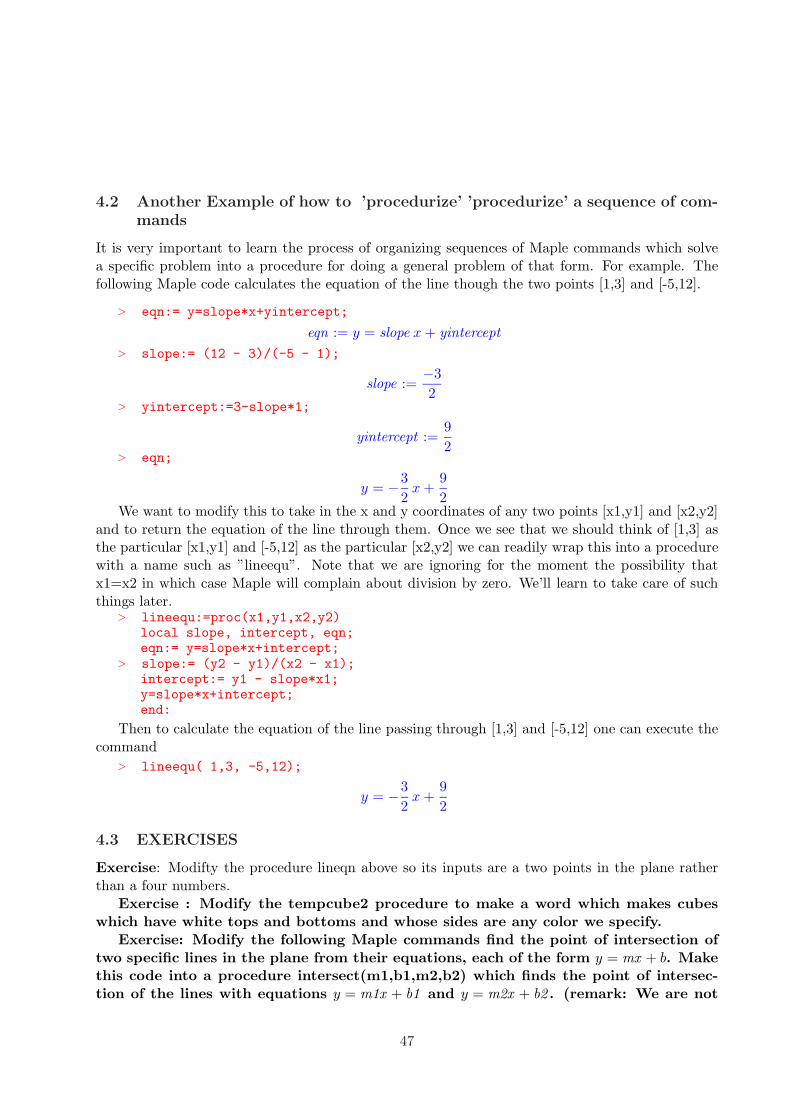
4.2 Another Example of how to ’procedurize’ ’procedurize’ a sequence of com-mands

It is very important to learn the process of organizing sequences of Maple commands which solvea specific problem into a procedure for doing a general problem of that form. For example. Thefollowing Maple code calculates the equation of the line though the two points [1,3] and [-5,12].

> eqn:= y=slope*x+yintercept;

eqn := y = slope x + yintercept

> slope:= (12 - 3)/(-5 - 1);

slope :=−3

2> yintercept:=3-slope*1;

yintercept :=9

2> eqn;

y = −3

2x +

9

2We want to modify this to take in the x and y coordinates of any two points [x1,y1] and [x2,y2]

and to return the equation of the line through them. Once we see that we should think of [1,3] asthe particular [x1,y1] and [-5,12] as the particular [x2,y2] we can readily wrap this into a procedurewith a name such as ”lineequ”. Note that we are ignoring for the moment the possibility thatx1=x2 in which case Maple will complain about division by zero. We’ll learn to take care of suchthings later.

> lineequ:=proc(x1,y1,x2,y2)local slope, intercept, eqn;eqn:= y=slope*x+intercept;

> slope:= (y2 - y1)/(x2 - x1);intercept:= y1 - slope*x1;y=slope*x+intercept;end:

Then to calculate the equation of the line passing through [1,3] and [-5,12] one can execute thecommand

> lineequ( 1,3, -5,12);

y = −3

2x +

9

2

4.3 EXERCISES

Exercise: Modifty the procedure lineqn above so its inputs are a two points in the plane ratherthan a four numbers.

Exercise : Modify the tempcube2 procedure to make a word which makes cubeswhich have white tops and bottoms and whose sides are any color we specify.

Exercise: Modify the following Maple commands find the point of intersection oftwo specific lines in the plane from their equations, each of the form y = mx + b. Makethis code into a procedure intersect(m1,b1,m2,b2) which finds the point of intersec-tion of the lines with equations y = m1x + b1 and y = m2x + b2 . (remark: We are not

47

worrying at this point about such niceties as whether the two lines are parallel or not.We will learn to check for this sort of thing later). Test your word on several lines.

> m1:=10: b1:=13: m2:=7: b2:=25:solve({y=m1*x+b1,y=m2*x+b2},{x,y});

{x = 4, y = 53}

Exercise : The Maple command sum(i,i=1..4781); adds up the first 4781 positiveintegers. Adapt it to make a Maple word addpowers(n,m) which returns the sum ofthe nth powers of the integers from 1 to m. Use your word to answer the followingquestion: Which is larger, the sum of the 4th powers of the first 100 positive integers,or the sum of the third powers of the first 300 integers?

Exercise: What does the following Maple procedure do? the word evalf is unfamiliar, use?evalf to get the help page (or use Maple Help at the top) .

> ndigitsPi:=proc(n) local tmp:Digits:=n; tmp:=evalf(Pi); Digits:=10: tmp;end:

Exercise: The following is a Maple procedure which almost works. It should inputa list of four numbers and make a bar graph representation of that data with the barrepresenting the first number having as it base the line segment [0,1] on the x-axis,the bar representing the second number should have as its base the segment [1,2], etc.The color of the first bar should be red, the second green, the third yellow, and thefourth blue.

> barit:=proc(l) local bar1,bar2,bar3, bar4;bar1:=plots[polygonplot]( [[2,0],[4,0],[4,l[3]],[2,l[3]]],color=green):

> bar2:=plots[polygonplot]( [[0,0],[1/2,0],[1/2,l[4]],[0,l[4]]],style=patch,color=red):bar3:=plots[polygonplot]( [[3,1],[5,1], [5,l[1]],[3,l[1]]],

> style=LINE,color=blue,thickness=3):bar4:=plots[polygonplot]( [[5,0],[6,0],[6,-l[2]],[5,-l[2]]],style=patch,color=yellow):plots[display]([bar1,bar2,bar3,bar4]); end;

Here is barit([5,2,7,-4])

\textbf{Exercise}: The following Maple procedure is supposed to inputthree points in the plane and check to see if they are collinear. Readthe instructions carefully and explain exactly what the procedure isdoing.

> checkit:=proc(P,Q,R) local slope, intercept, eqn;eqn:= y=slope*x+intercept;slope:= (Q[2] - P[2])/(Q[1] - P[1]);

> intercept:= Q[2] - slope*Q[1];R[2]=slope*R[1]+interceptend;

48

Exercise: The following procedure inputs a list of four points in the plane and does a calculationwhich hopes to tell whether the four points are the vertices of a square. Draw a diagram of aquadralateral, label the vertices in accordance with the notation used by the procedure and explainwith reference to the geometry of the figure exactly what the procedure is doing. Explain why itsoutput can or can not tell one whether the figure is in fact a square

Recall that if P is a list of things that are themselves lists then P[3,7] denotes the seventhelement of the third member of the list P.

> isit:=proc( P) local tmp1,tmp2:tmp1:= ((P[1,1]-P[3,1])^2 + ( P[1,2]-P[3,2])^2) - ((P[2,1]-P[4,1])^2 + (

> P[2,2]-P[4,2])^2 );tmp2:= ((P[1,1]-P[2,1])^2 + ( P[1,2]-P[2,2])^2) - ( (P[2,1]-P[3,1])^2+ (

> P[2,2]-P[3,2])^2 );tmp1^2+tmp2^2;end:

49

5 Laying Bricks:Getting the Computer to do Repetitive Tasks

5.1 Working with expression sequences and lists

The process of analyzing or solving a problem can involve a lot of repetition. Anyone who hasgraphed many different functions knows the tedious repetition of that process. Maple’s built-in”plot” commands allow the computer do the mindless repetition, freeing time for people to look atthe relationships implied by the graph - something the machine can’t do. Graphing, however is onlyone example of this of this capability which is absolutely critical to effective use of the computerfor solving general problems. Lets look at another - building lists.

We have already made and used a lot of Maple lists. A more primitive notion than that of alist is that of an expression sequence

Definition: An expression sequence is a comma-separated expression of the form ”a,b,c,...,z”where the elements ”a”, ”b” , etc. can be any symbols recognizable by Maple.

The order of elements in an expression sequence is important: ”a,b” is a different expressionsequence from ”b,a”

For our immediate purposes the most important thing about expression sequences is how easyit is to extend them. If joe is an expression sequence and we want to add ”Hortense” to the end ofjoe we can simply enter joe:=joe, Hortense; . If we wanted to place Hortense at the beginningwe would enter joe:= Hortense,joe; This idea also allows us to ”build” sequences.

If we initially have a sequence named ”joe” and need, in the course of a calculation to extend”joe” then this can be done through steps like

> joe:=I;

joe := I

> joe:=joe,like;

joe := I, like

> joe:=joe,math;

Sometimes it is useful as a starting point to have an empty expression. That is something whichis an expression but has no items in it. This is evidently analogous to the empty set in set theory.This idea is so useful that Maple has a special name for the emptyexpression sequence. It is calledNULL....

joe := I, like, math

> joe:=NULL;

joe :=

> joe:=joe,I;

joe := I

> joe:=joe,like;

joe := I, like

> joe:=joe,math;

joe := I, like, math

50

With the notion of expression sequence we can observe that a list is simply an expressionsequence delimited by brackets ”[ ]”. Most important, to convert an expression sequence, joeto a list sam we simply enclose it in brackets

> sam:=[joe];

sam := [I, like, math ]

Since a list is simply an expression sequence enclosed in brackets there is a simple way to extractthe undellying expression sequence from a list with a command called op. We will encounter opquite often. This is but one of its many uses. ( op stands for operands )

5.2 How to Build a list by hand

Maple has a word whattype which we can use to ask what type it has assigned to various objects(there are many kinds of types). Now let’s illustrate.

First let’s make a simple sequence. We will start with the NULL sequence to indicate how it isused as a starting point for building sequences

> joe:=NULL;

joe :=

> harry:=joe,sally,1;

harry := sally , 1

> whattype(joe);

exprseq

> whattype(harry);

exprseq

> joe:= harry,dog, Pi;

joe := sally , 1, dog , π

> whattype(joe);

exprseq

> sam:=[joe];

sam := [sally , 1, dog , π]

> whattype(sam);

list

> tim:=op(sam);

tim := sally , 1, dog , π

> whattype(tim);

exprseq

Now suppose we want to make the list stuff:= [sally,1,dog, π, Lance]; . We observe that

51

we should be able to do this simply by adding ”Lance” to the end of the list ”sam”. We wouldlike to do something like stuff:=sam,Lance; or stuff:=[sam,Lance]; but neither of these willwork. This is not to say that Maple won’t accept the commands

> stuff:=sam,Lance;

stuff := [sally , 1, dog , π], Lance

> whattype(stuff);

exprseq

> stuff:=[sam,Lance];

stuff := [[sally , 1, dog , π], Lance ]

Neither of these works. The first produces an expression sequence, not a list. Moreover it hasonly two elements, the first being the list ”sam” and and the second the expression ”Lance”. Thesecond does produce a list but it is a list with two elements: the first element of this is the list ”[sally,1,dog, π]” and the second is ”Lance”.

In order to produce the list we want we have to extract the expression sequence from ”sam”,append ”Lance ” to it and then convert that sequence to a list.

> tmp:=op(sam);

tmp := sally , 1, dog , π

> tmp:=tmp,Lance;

tmp := sally , 1, dog , π, Lance

> stuff:=[tmp];

stuff := [sally , 1, dog , π, Lance]

> whattype(stuff);

list

We can be more economical by combining steps by composing commands:

> stuff:=[op(sam),Lance];

stuff := [sally , 1, dog , π, Lance]

Incidentally, to go with ”op” there is a very useful commnad nops (number of operands)which we can use to tell us how many items there are in a list

> junk:=[a,b,cow];

junk := [a, b, cow ]

> nops(junk);

3

Note that nops doesn’t work on an expression sequence.> nops(NULL);

Error, wrong number (or type) of parameters in function nops

> sally:=1,2,3;

52

sally := 1, 2, 3

> nops(sally);

Error, wrong number (or type) of parameters in function nops

Thus in order to count the number of items in an expression sequence we must ask nops to acton a list of which the expression sequence is the operand.

> sally:=1,2,3;

sally := 1, 2, 3

> nops([sally]);

3

> whattype(sally);

exprseq

It is important to note that writing ”[sally]” above does not change ”sally” into a list. Theassignment command sally:=[sally]; would do that but above we have not assigned a new value to”sally”. All we have done is ask nops to act on an unnamed list constructed from ”sally”. This leadsto a comment we must make regarding what happens when we make an expression sequence someof whose elements are objects that have assigned values. For instance suppose we have executedbird:=turkey; and subsequently make an expressions sequence animals:=cat,dog,bird; Thesequence animals will then be cat,dog,turkey. That is, the value that has been assigned to any ofthe terms in the sequence we write down will be substituted immediately. If we then redefine ”bird”,say bird:=pigeon; the sequence animals will still be cat,dog,turkey unless we do somethingwhich re-defines animals (e.g. we might re-execute the command animals:=cat,dog,bird; atwhich time animals will become cat,dog,pigeon .

> bird:=turkey;

bird := turkey

> animals:=cat,dog,bird;

animals := cat , dog , turkey

> print([animals]);

[cat , dog , turkey ]

> bird:=pigeon;

bird := pigeon

> print([animals]);

[cat , dog , turkey ]

> animals:=cat,dog,bird;

animals := cat , dog , pigeon

> print([animals]);

[cat , dog , pigeon ]

This property of sequences is extremely important for it allows us to build a sequence in steps

53

re-using a temporary name for the item we are adding.

> dogs:=NULL;

dogs :=

> tmpdog:=Beagle;

tmpdog := Beagle

> dogs:=dogs,tmpdog;

dogs := Beagle

> tmpdog:=Airdale;

tmpdog := Airdale

> dogs:=dogs,tmpdog;

dogs := Beagle , Airdale

5.3 Automatically Generating Sequences and Lists

Now suppose we wanted to make a list of the first 25 positive intgers. One way to do this is simplyto enter it:

> numlist:=[1,2,3,4,5,6,7,8,9,10,11,12,13,14,15,17,17,18,19,20,21,22,23,24,24,25];

numlist := [1, 2, 3, 4, 5, 6, 7, 8, 9, 10, 11, 12, 13, 14, 15, 17, 17, 18, 19, 20, 21, 22, 23, 24,

24, 25]

This is tedious and fraught with opportunity to make mistakes. Indeed the careful reader willhave noted that this isn’t the correct list, ”17” was entered twice. Even that careful soul mightnot take the time to check whether this sequence which clams to list the numbers from 672345 to677345 is actually correct.

5.3.1 Boring List of Numbers from 672345 To 677345

boringlist := [672345, 672346, 672347, 672348, 672349, 672350, 672351, 672352,672353, 672354, 672355, 672356, 672357, 672358, 672359, 672360, 672361, 672362,672363, 672364, 672365, 672366, 672367, 672368, 672369, 672370, 672371, 672372,672373, 672374, 672375, 672376, 672377, 672378, 672379, 672380, 672381, 672382,672383, 672384, 672385, 672386, 672387, 672388, 672389, 672390, 672391, 672392,672393, 672394, 672395, 672396, 672397, 672398, 672399, 672400, 672401, 672402,672403, 672404, 672405, 672406, 672407, 672408, 672409, 672410, 672411, 672412,672413, 672414, 672415, 672416, 672417, 672418, 672419, 672420, 672421, 672422,672423, 672424, 672425, 672426, 672427, 672428, 672429, 672430, 672431, 672432,672433, 672434, 672435, 672436, 672437, 672438, 672439, 672440, 672441, 672442,672443, 672444, 672445, 672446, 672447, 672448, 672449, 672450, 672451, 672452,672453, 672454, 672455, 672456, 672457, 672458, 672459, 672460, 672461, 672462,672463, 672464, 672465, 672466, 672467, 672468, 672469, 672470, 672471, 672472,

54

672473, 672474, 672475, 672476, 672477, 672478, 672479, 672480, 672481, 672482,672483, 672484, 672485, 672486, 672487, 672488, 672489, 672490, 672491, 672492,672493, 672494, 672495, 672496, 672497, 672498, 672499, 672500, 672501, 672502,672503, 672504, 672505, 672506, 672507, 672508, 672509, 672510, 672511, 672512,672513, 672514, 672515, 672516, 672517, 672518, 672519, 672520, 672521, 672522,672523, 672524, 672525, 672526, 672527, 672528, 672529, 672530, 672531, 672532,672533, 672534, 672535, 672536, 672537, 672538, 672539, 672540, 672541, 672542,672543, 672544, 672545, 672546, 672547, 672548, 672549, 672550, 672551, 672552,672553, 672554, 672555, 672556, 672557, 672558, 672559, 672560, 672561, 672562,672563, 672564, 672565, 672566, 672567, 672568, 672569, 672570, 672571, 672572,672573, 672574, 672575, 672576, 672577, 672578, 672579, 672580, 672581, 672582,672583, 672584, 672585, 672586, 672587, 672588, 672589, 672590, 672591, 672592,672593, 672594, 672595, 672596, 672597, 672598, 672599, 672600, 672601, 672602,672603, 672604, 672605, 672606, 672607, 672608, 672609, 672610, 672611, 672612,672613, 672614, 672615, 672616, 672617, 672618, 672619, 672620, 672621, 672622,672623, 672624, 672625, 672626, 672627, 672628, 672629, 672630, 672631, 672632,672633, 672634, 672635, 672636, 672637, 672638, 672639, 672640, 672641, 672642,672643, 672644, 672645, 672646, 672647, 672648, 672649, 672650, 672651, 672652,672653, 672654, 672655, 672656, 672657, 672658, 672659, 672660, 672661, 672662,672663, 672664, 672665, 672666, 672667, 672668, 672669, 672670, 672671, 672672,672673, 672674, 672675, 672676, 672677, 672678, 672679, 672680, 672681, 672682,672683, 672684, 672685, 672686, 672687, 672688, 672689, 672690, 672691, 672692,672693, 672694, 672695, 672696, 672697, 672698, 672699, 672700, 672701, 672702,672703, 672704, 672705, 672706, 672707, 672708, 672709, 672710, 672711, 672712,672713, 672714]

”boringlist” is actually correct because it was not typed in by hand but rather done by a Maplecommand seq which generates expression sequences according to a ”formula” we prescribe whichtells Maple how to find the ”nth” element. A few examples suffice to illustrate this very usefulcommand. First, here is the command that generated ”boringlist”

> boringlist:=[seq(i,i=672345..672714)];

Note that seq returns an expression sequence. The brackets in turn make that a list. Anexpression sequence of the cubes of the integers from -3 to 13 is simply

> cubesequence:=seq(i^3,i=-3..13);

cubesequence :=

−27, −8, −1, 0, 1, 8, 27, 64, 125, 216, 343, 512, 729, 1000, 1331, 1728, 2197

We can convert it into a list

> cubelist:=[cubesequence];

cubelist := [−27, −8, −1, 0, 1, 8, 27, 64, 125, 216, 343, 512, 729, 1000, 1331, 1728, 2197]

if the list was all we wanted we could have skipped naming the sequence and simply entered> cubelist:=[seq(i^3,i=-3..13)];

55

cubelist := [−27, −8, −1, 0, 1, 8, 27, 64, 125, 216, 343, 512, 729, 1000, 1331, 1728, 2197]

Some further examples of lists:

Make a list if the odd integers from 1 to 99

> oddlist:=[seq( 2*j+1,j=0..49)];

oddlist := [1, 3, 5, 7, 9, 11, 13, 15, 17, 19, 21, 23, 25, 27, 29, 31, 33, 35, 37, 39, 41, 43, 45,

47, 49, 51, 53, 55, 57, 59, 61, 63, 65, 67, 69, 71, 73, 75, 77, 79, 81, 83, 85, 87, 89,

91, 93, 95, 97, 99]

Make an expression sequence of all the natural numbers less than 137 which are 2 plus a multipleof 7.

> twomodsevenseq:=seq(2+7*q,q=0..137/7);

twomodsevenseq :=

2, 9, 16, 23, 30, 37, 44, 51, 58, 65, 72, 79, 86, 93, 100, 107, 114, 121, 128, 135

Make a list of lists of numbers so that the nth element in your list is the list [n, 1n2 ], starting

with n=10 and ending with n=30.

> listoflists:=[seq([n,1/n^2],n=10..30)];

listoflists := [[10,1

100], [11,

1

121], [12,

1

144], [13,

1

169], [14,

1

196], [15,

1

225], [16,

1

256],

[17,1

289], [18,

1

324], [19,

1

361], [20,

1

400], [21,

1

441], [22,

1

484], [23,

1

529], [24,

1

576],

[25,1

625], [26,

1

676], [27,

1

729], [28,

1

784], [29,

1

841], [30,

1

900]]

5.4 Exercises: Sequences and Lists

Exercise: Make a list of all the natural numbers which are less than 1000 and are thesquare of another natural number.

Exercise: Make a sequence of length 100 such that the jth element of list whose first elementis the integer j and who second element is the factorization of j into primes.

Exercise: Make a list of length 5 whose jth element is a plot of the function sin(j*x) on theinterval [0, 2π]. Display all of the graphs at once with plots[display].

Exercise: Make a sequence of 100 random integrers between 0 and 10. ( If necessary, use”help” to look up the topic ”random”).

Exercise: If ”n” is a natural number then n factorial, denoted ”n!” is the productn(n-1)(n-2)... (3)(2)(1). For instance 3!=(3)(2)(1) = 6, 1! = 1, 4!=(4)(3)(2)(1) =24. Maple recognizes the notation n! and will compute the factorial of a natural number.Make a list of the factorials of the numbers from 1 to 20.

56

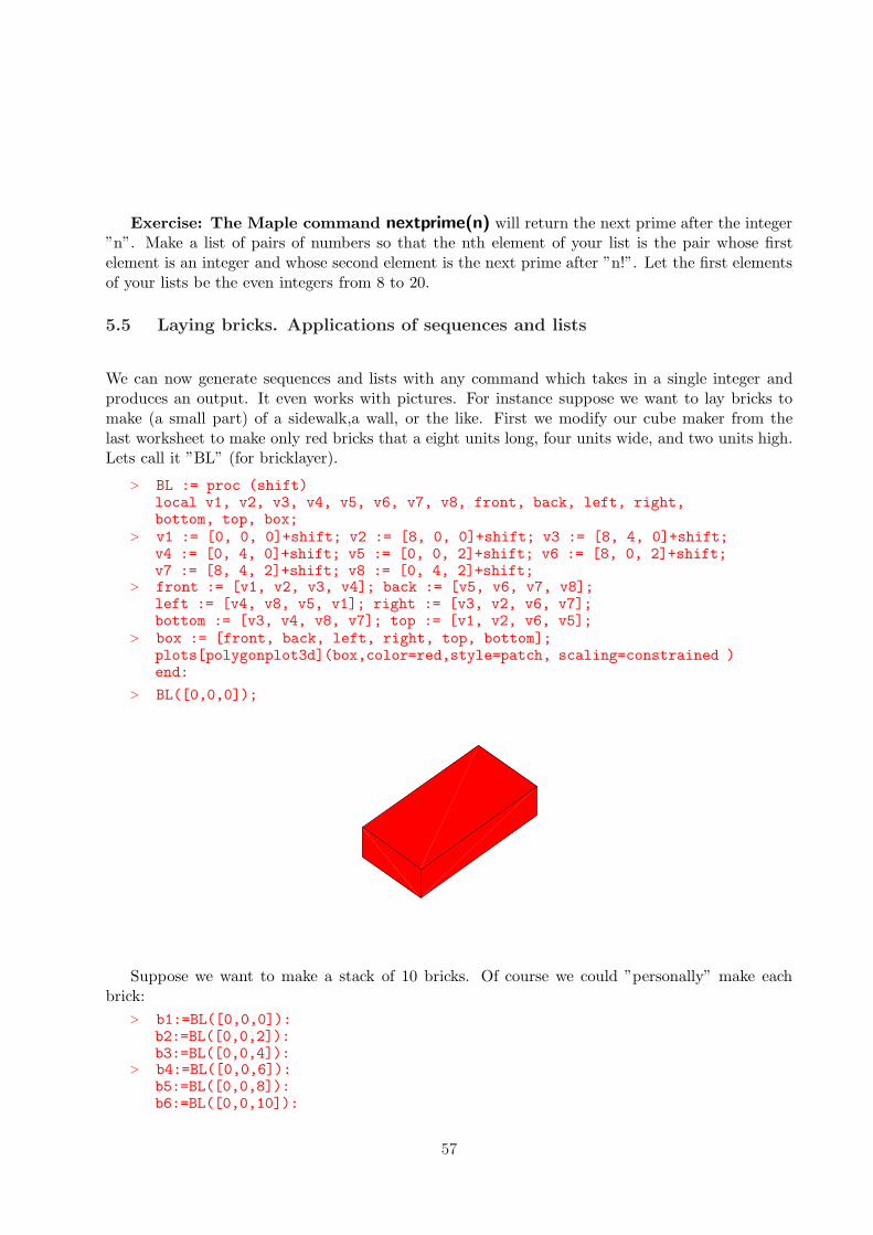
Exercise: The Maple command nextprime(n) will return the next prime after the integer”n”. Make a list of pairs of numbers so that the nth element of your list is the pair whose firstelement is an integer and whose second element is the next prime after ”n!”. Let the first elementsof your lists be the even integers from 8 to 20.

5.5 Laying bricks. Applications of sequences and lists

We can now generate sequences and lists with any command which takes in a single integer andproduces an output. It even works with pictures. For instance suppose we want to lay bricks tomake (a small part) of a sidewalk,a wall, or the like. First we modify our cube maker from thelast worksheet to make only red bricks that a eight units long, four units wide, and two units high.Lets call it ”BL” (for bricklayer).

> BL := proc (shift)local v1, v2, v3, v4, v5, v6, v7, v8, front, back, left, right,bottom, top, box;

> v1 := [0, 0, 0]+shift; v2 := [8, 0, 0]+shift; v3 := [8, 4, 0]+shift;v4 := [0, 4, 0]+shift; v5 := [0, 0, 2]+shift; v6 := [8, 0, 2]+shift;v7 := [8, 4, 2]+shift; v8 := [0, 4, 2]+shift;

> front := [v1, v2, v3, v4]; back := [v5, v6, v7, v8];left := [v4, v8, v5, v1]; right := [v3, v2, v6, v7];bottom := [v3, v4, v8, v7]; top := [v1, v2, v6, v5];

> box := [front, back, left, right, top, bottom];plots[polygonplot3d](box,color=red,style=patch, scaling=constrained )end:

> BL([0,0,0]);

Suppose we want to make a stack of 10 bricks. Of course we could ”personally” make eachbrick:

> b1:=BL([0,0,0]):b2:=BL([0,0,2]):b3:=BL([0,0,4]):

> b4:=BL([0,0,6]):b5:=BL([0,0,8]):b6:=BL([0,0,10]):

57

> b7:=BL([0,0,12]):b8:=BL([0,0,14]):b9:=BL([0,0,16]):b10:=BL([0,0,18]):

Then we produce a list to feed to plots[display] . Note that we terminate with a semicolon.The reader might want to change it to a colon and execute the command to remind him/herselfwhy - then change it back to a colon and execute again.

> tenbricks:=[b1,b2,b3,b4,b5,b6,b7,b8,b9,b10]:

Now we can look at the picture:> plots[display](tenbricks);

We observe that what we are doing is in making the nth brick is just BL([0,0,2*n]); and thisdepends only on the integer ”n” (we are starting with n=0). So to get our list all we need do isthe following. Again we terminate with a colon ”:” as we don’t want to see the list in this form -we only want the picture.

> bricklist:=[seq(BL([0,0,2*n]),n=0..9)]:plots[display](bricklist);

We can improve even further with a compound command which simply combines the previoussteps

> plots[ display ]([ seq(BL([0,0,2*n]), n=0..9) ]);

58

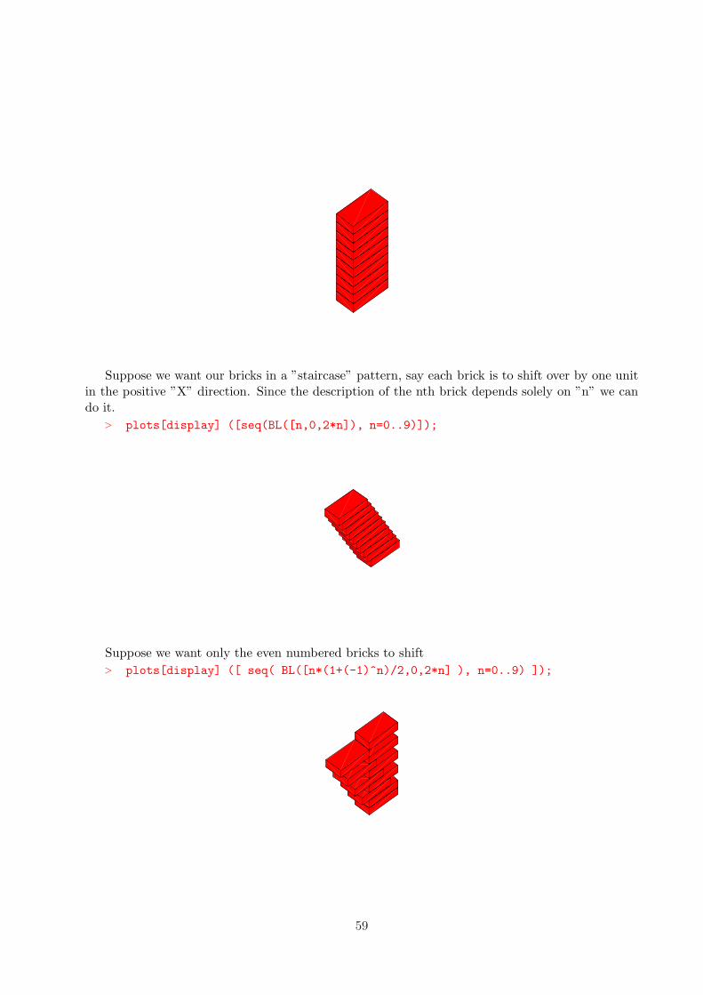
Suppose we want our bricks in a ”staircase” pattern, say each brick is to shift over by one unitin the positive ”X” direction. Since the description of the nth brick depends solely on ”n” we cando it.

> plots[display] ([seq(BL([n,0,2*n]), n=0..9)]);

Suppose we want only the even numbered bricks to shift> plots[display] ([ seq( BL([n*(1+(-1)^n)/2,0,2*n] ), n=0..9) ]);

59

5.6 EXERCISES: Making Brick Patterns With seq

Exercise: Stack the ten bricks in so that they shift both in the ”X” and ”Y” directions,making each brick after the first shift 1/3 of a unit in the positive ”X” direction and1/4 of a unit in the negative ”Y” direction.

Exercise: Stack the ten bricks so that they don’t shift in the ”Y” direction butwe want each odd numbered brick to be shifted 1 units more than the previous oddnumbered brick in the positive ”X” direction and the ith even numbered brick tobe shifted 1 unit more than the previous even-numbered brick in the negative ”X”direction.

Exercise: Using the ”seq” command place the ten bricks so that are end to end.

Exercise: Using the ”seq” command place the ten bricks so that they are in arectangular pattern of five rows and two columns.

60

6 Stacking Colored Bricks:

An Introduction to for .. do ... od and if ... then ...fiCommands.

6.1 A Chromatic Brick Placer

Suppose we want to stack ten bricks but we want to alternate the colors. First we need to restorethe color option to our ”BL” command. Lets modify it to a ”CBP” (chromatic brick placer) whichallows us to specify the color.

> CBP:= proc (shift,clr )local v1, v2, v3, v4, v5, v6, v7, v8, front, back, left, right,bottom, top, box;



> box := [front, back, left, right, top, bottom];plots[polygonplot3d](box,color=clr,style=patch, scaling=constrained )end:

> plots[display]([CBP([0,0,0],blue),CBP([0,0,2],white),CBP([0,0,4],red)]);

Suppose we want to stack alternating blue and red bricks. The obvious way to do it ”by hand”would be to manufacture the bricks one at a time assemble them into a list and use plots[display]to view the result. Indeed lets do a few steps in the process to see what we want to automate. Thistime we want to assemble the list as we go rather than waiting until the end. This should keep usfrom having to give a permanent name to each one. We simply give each new brick a temporaryname and append it to the list. Lets let ”CBS” stand for colored brick stack.

> CBS:=NULL:tmpbrick:=CBP([0,0,0],red):CBS:=CBS,tmpbrick:tmpbrick:=CBP([0,0,2],blue):

61

> CBS:=CBS,tmpbrick:tmpbrick:=CBP([0,0,4],red):CBS:=CBS,tmpbrick:

> tmpbrick:=CBP([0,0,6],blue):CBS:=CBS,tmpbrick:

> plots[display]([CBS]);

Like the other processes we have been working with recently we can see that this is terriblyrepetetive. All we are doing is repeating the two commands

tmpbrick =CBP([0,0,x], somecolor); CBS:=CBS,tmpbrick;and we are doing it ten times.What we need is the ability to tell the computer to do something a fixed number of times - in

this case 10 times. The basic format for the command that does this isfor VARIABLE from STARTINGNUMBER to STOPPING NUMBER do ”sequence of Maple

Commands” od;You can always spot the end of a do statement with do spelled backwards. od

To have Maple print ”[n,n!]” for n from 1 to 10 one could do the following

> for n from 1 to 10 do [n, n!] od;

[1, 1]

[2, 2]

[3, 6]

[4, 24]

[5, 120]

[6, 720]

[7, 5040]

[8, 40320]

[9, 362880]

[10, 3628800]

62

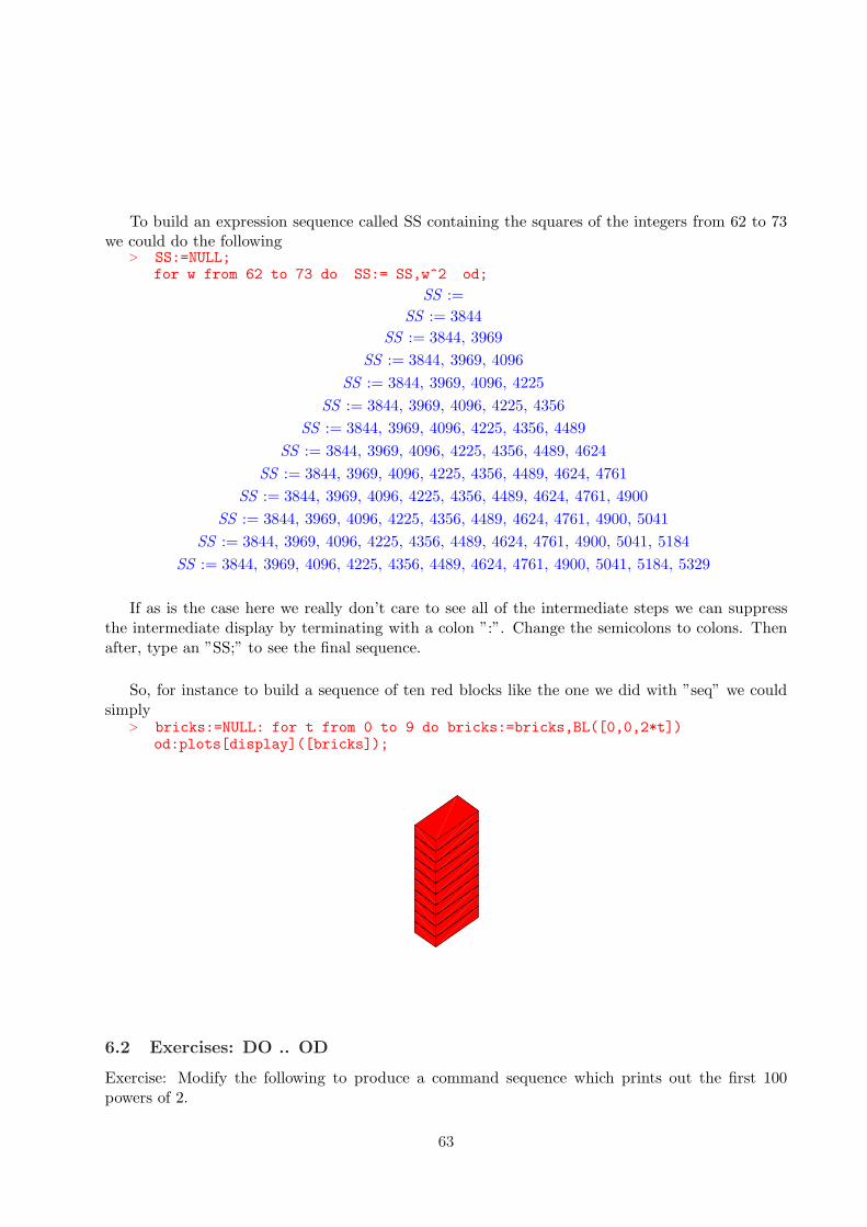
To build an expression sequence called SS containing the squares of the integers from 62 to 73we could do the following

> SS:=NULL;for w from 62 to 73 do SS:= SS,w^2 od;

SS :=

SS := 3844

SS := 3844, 3969

SS := 3844, 3969, 4096

SS := 3844, 3969, 4096, 4225

SS := 3844, 3969, 4096, 4225, 4356

SS := 3844, 3969, 4096, 4225, 4356, 4489

SS := 3844, 3969, 4096, 4225, 4356, 4489, 4624

SS := 3844, 3969, 4096, 4225, 4356, 4489, 4624, 4761

SS := 3844, 3969, 4096, 4225, 4356, 4489, 4624, 4761, 4900

SS := 3844, 3969, 4096, 4225, 4356, 4489, 4624, 4761, 4900, 5041

SS := 3844, 3969, 4096, 4225, 4356, 4489, 4624, 4761, 4900, 5041, 5184

SS := 3844, 3969, 4096, 4225, 4356, 4489, 4624, 4761, 4900, 5041, 5184, 5329

If as is the case here we really don’t care to see all of the intermediate steps we can suppressthe intermediate display by terminating with a colon ”:”. Change the semicolons to colons. Thenafter, type an ”SS;” to see the final sequence.

So, for instance to build a sequence of ten red blocks like the one we did with ”seq” we couldsimply

> bricks:=NULL: for t from 0 to 9 do bricks:=bricks,BL([0,0,2*t])od:plots[display]([bricks]);

6.2 Exercises: DO .. OD

Exercise: Modify the following to produce a command sequence which prints out the first 100powers of 2.

63

> for x from 0 to 5 do print(x,2*x) od;

0, 0

1, 2

2, 4

3, 6

4, 8

5, 10

Exercise: Write a command sequence which prints out [n, (1 + 1n)n] for the first 100 values of

n.

6.3 Conditional statements

Now we would like to make a stack of differently colored bricks. We will use our ”CBP” commandin a do .. od constructionl but we need to add commands within the ”loop” to tell Maple howto color the tiles. Suppose we want to start with a red brick on the bottom and then alternatewith blue blocks from then. We need a way to issue the following instructions to the computer.”if t is even then make the brick red otherwise make it blue”. We do this with the if ... then ...else .. fi command. Just as we end the do statement with do spelled backwards an if..then ..statement is ended with if spelled backwards. Like the do..od command the if..fi command isbest explained with an example. Lets do the alternating red-blue bricks. There are lots of possibleways to do this. We will be very pedantic at first. We need one additional tool. First recall that aninteger is even if it yields a remainder of zero when divided by 2; it is odd if it leaves a remainder of1 under the same circumstances. If we enter the command ”a mod b;” Maple returns the remainderupon division of ”a” by ”b”.

> 34 mod 12;

10

> 17 mod 3;

2

Now let ”T” have some integral value and lets test whether its even or odd and make a red orblue brick accordingly

> T:=17;

T := 17

> if T mod 2 = 1 then CBP([0,0,0],red) else CBP([0,0,0],blue) fi;

64

> T:=18;

T := 18

> if T mod 2 = 1 then CBP([0,0,0],red) else CBP([0,0,0],blue) fi ;

Note that it is often convenient to enclose expressions of the form a mod b in parenthesis.This is optional but it tends to make Maple code easier to follow. Be especially careful to distinguishthe equality = symbol in the above as opposed to the assignment symbol := . Although theselook similar they are miles apart. The statement T := 17; assigns the value 17 to the name T.The equation T mod 2 = 1 is tested in the if .. fi statements above. Now all we have to do ismodify the ”body” of our ”do..od” command which stacked ten red bricks

> bricks:=NULL:for t from 0 to 9 doif (t mod 2) = 1 then

> tmpbrick:=CBP([0,0,2*t],red) elsetmpbrick:=CBP([0,0,2*t],blue) fi:bricks:=bricks,tmpbrick; od:plots[display]([bricks]);

65

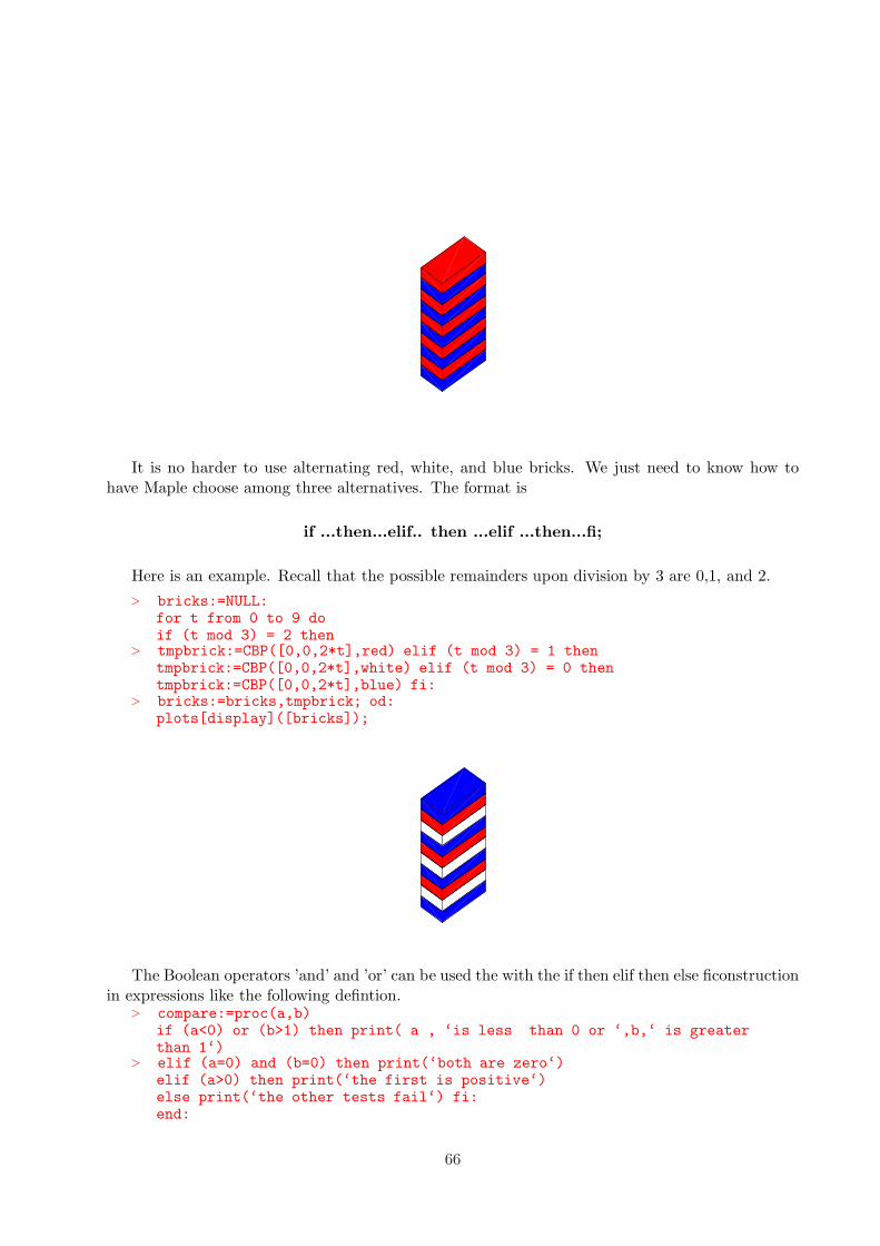
It is no harder to use alternating red, white, and blue bricks. We just need to know how tohave Maple choose among three alternatives. The format is

if ...then...elif.. then ...elif ...then...fi;

Here is an example. Recall that the possible remainders upon division by 3 are 0,1, and 2.

> bricks:=NULL:for t from 0 to 9 doif (t mod 3) = 2 then

> tmpbrick:=CBP([0,0,2*t],red) elif (t mod 3) = 1 thentmpbrick:=CBP([0,0,2*t],white) elif (t mod 3) = 0 thentmpbrick:=CBP([0,0,2*t],blue) fi:

> bricks:=bricks,tmpbrick; od:plots[display]([bricks]);

The Boolean operators ’and’ and ’or’ can be used the with the if then elif then else ficonstructionin expressions like the following defintion.

> compare:=proc(a,b)if (a<0) or (b>1) then print( a , ‘is less than 0 or ‘,b,‘ is greaterthan 1‘)

> elif (a=0) and (b=0) then print(‘both are zero‘)elif (a>0) then print(‘the first is positive‘)else print(‘the other tests fail‘) fi:end:

66

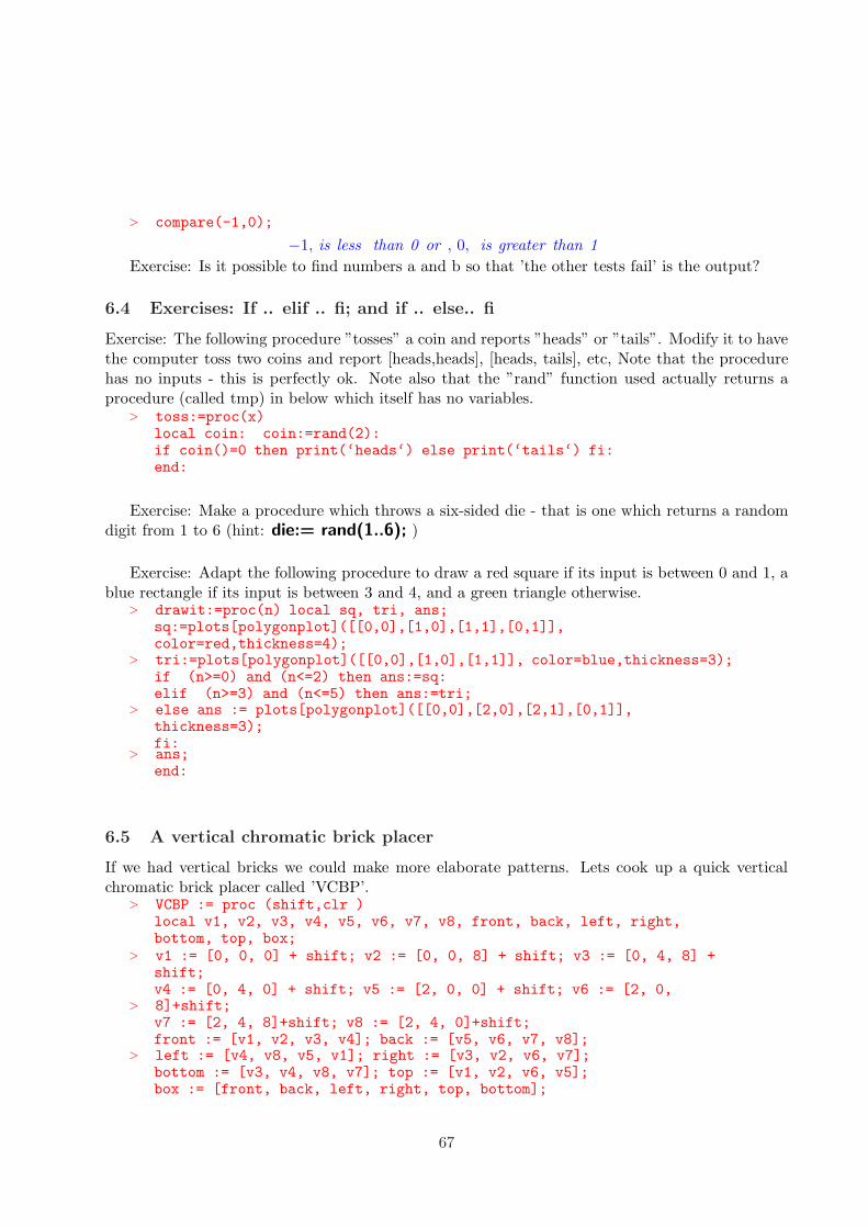
> compare(-1,0);

−1, is less than 0 or , 0, is greater than 1

Exercise: Is it possible to find numbers a and b so that ’the other tests fail’ is the output?

6.4 Exercises: If .. elif .. fi; and if .. else.. fi

Exercise: The following procedure ”tosses” a coin and reports ”heads” or ”tails”. Modify it to havethe computer toss two coins and report [heads,heads], [heads, tails], etc, Note that the procedurehas no inputs - this is perfectly ok. Note also that the ”rand” function used actually returns aprocedure (called tmp) in below which itself has no variables.

> toss:=proc(x)local coin: coin:=rand(2):if coin()=0 then print(‘heads‘) else print(‘tails‘) fi:end:

Exercise: Make a procedure which throws a six-sided die - that is one which returns a randomdigit from 1 to 6 (hint: die:= rand(1..6); )

Exercise: Adapt the following procedure to draw a red square if its input is between 0 and 1, ablue rectangle if its input is between 3 and 4, and a green triangle otherwise.

> drawit:=proc(n) local sq, tri, ans;sq:=plots[polygonplot]([[0,0],[1,0],[1,1],[0,1]],color=red,thickness=4);

> tri:=plots[polygonplot]([[0,0],[1,0],[1,1]], color=blue,thickness=3);if (n>=0) and (n<=2) then ans:=sq:elif (n>=3) and (n<=5) then ans:=tri;

> else ans := plots[polygonplot]([[0,0],[2,0],[2,1],[0,1]],thickness=3);fi:

> ans;end:

6.5 A vertical chromatic brick placer

If we had vertical bricks we could make more elaborate patterns. Lets cook up a quick verticalchromatic brick placer called ’VCBP’.

> VCBP := proc (shift,clr )local v1, v2, v3, v4, v5, v6, v7, v8, front, back, left, right,bottom, top, box;

> v1 := [0, 0, 0] + shift; v2 := [0, 0, 8] + shift; v3 := [0, 4, 8] +shift;v4 := [0, 4, 0] + shift; v5 := [2, 0, 0] + shift; v6 := [2, 0,

> 8]+shift;v7 := [2, 4, 8]+shift; v8 := [2, 4, 0]+shift;front := [v1, v2, v3, v4]; back := [v5, v6, v7, v8];

> left := [v4, v8, v5, v1]; right := [v3, v2, v6, v7];bottom := [v3, v4, v8, v7]; top := [v1, v2, v6, v5];box := [front, back, left, right, top, bottom];

67

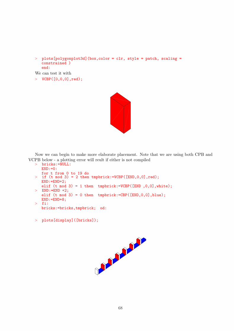
> plots[polygonplot3d](box,color = clr, style = patch, scaling =constrained )end:

We can test it with

> VCBP([0,0,0],red);

Now we can begin to make more elaborate placement. Note that we are using both CPB andVCPB below - a plotting error will reult if either is not compiled

> bricks:=NULL:END:=0:for t from 0 to 19 do

> if (t mod 3) = 2 then tmpbrick:=VCBP([END,0,0],red);END:=END+2;elif (t mod 3) = 1 then tmpbrick:=VCBP([END ,0,0],white);

> END:=END +2;elif (t mod 3) = 0 then tmpbrick:=CBP([END,0,0],blue);END:=END+8;

> fi:bricks:=bricks,tmpbrick; od:

> plots[display]([bricks]);

68

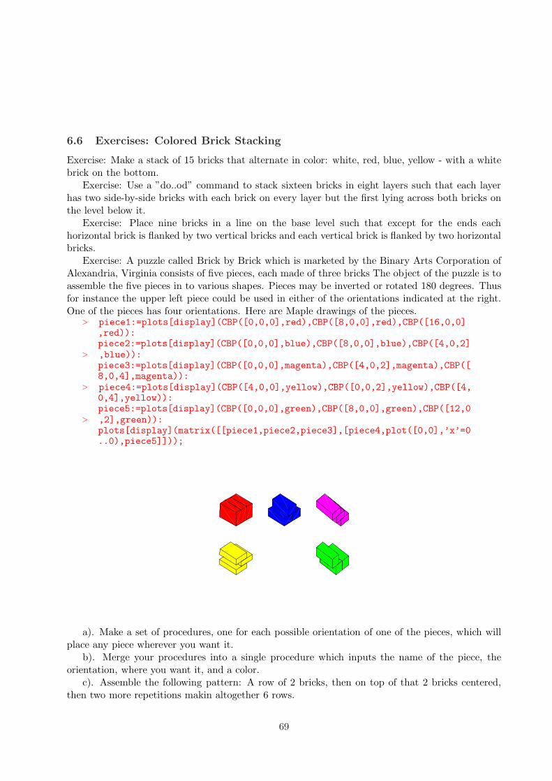
6.6 Exercises: Colored Brick Stacking

Exercise: Make a stack of 15 bricks that alternate in color: white, red, blue, yellow - with a whitebrick on the bottom.

Exercise: Use a ”do..od” command to stack sixteen bricks in eight layers such that each layerhas two side-by-side bricks with each brick on every layer but the first lying across both bricks onthe level below it.

Exercise: Place nine bricks in a line on the base level such that except for the ends eachhorizontal brick is flanked by two vertical bricks and each vertical brick is flanked by two horizontalbricks.

Exercise: A puzzle called Brick by Brick which is marketed by the Binary Arts Corporation ofAlexandria, Virginia consists of five pieces, each made of three bricks The object of the puzzle is toassemble the five pieces in to various shapes. Pieces may be inverted or rotated 180 degrees. Thusfor instance the upper left piece could be used in either of the orientations indicated at the right.One of the pieces has four orientations. Here are Maple drawings of the pieces.

> piece1:=plots[display](CBP([0,0,0],red),CBP([8,0,0],red),CBP([16,0,0],red)):piece2:=plots[display](CBP([0,0,0],blue),CBP([8,0,0],blue),CBP([4,0,2]

> ,blue)):piece3:=plots[display](CBP([0,0,0],magenta),CBP([4,0,2],magenta),CBP([8,0,4],magenta)):

> piece4:=plots[display](CBP([4,0,0],yellow),CBP([0,0,2],yellow),CBP([4,0,4],yellow)):piece5:=plots[display](CBP([0,0,0],green),CBP([8,0,0],green),CBP([12,0

> ,2],green)):plots[display](matrix([[piece1,piece2,piece3],[piece4,plot([0,0],’x’=0..0),piece5]]));

a). Make a set of procedures, one for each possible orientation of one of the pieces, which willplace any piece wherever you want it.

b). Merge your procedures into a single procedure which inputs the name of the piece, theorientation, where you want it, and a color.

c). Assemble the following pattern: A row of 2 bricks, then on top of that 2 bricks centered,then two more repetitions makin altogether 6 rows.

69

d). Why can’t you have a pattern like the one in c) except it is 8 rows high?

70

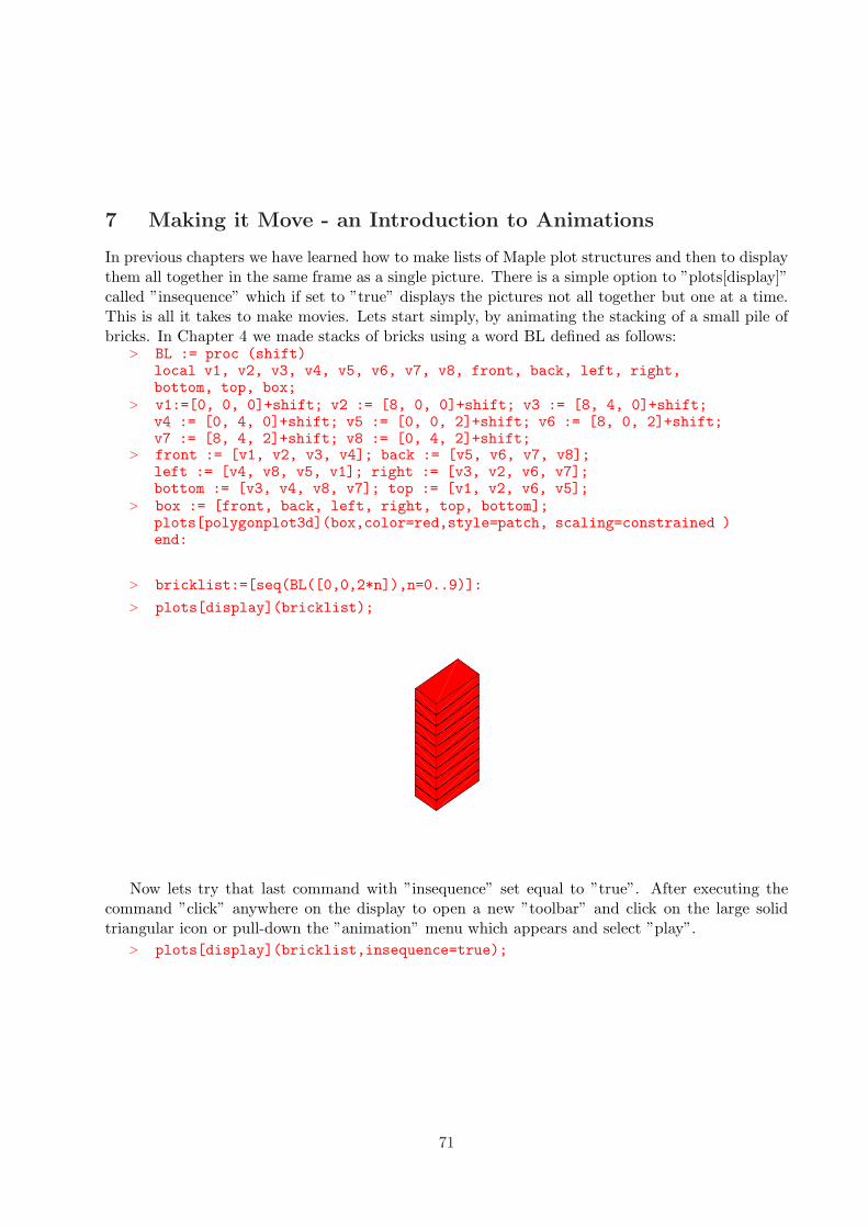
7 Making it Move - an Introduction to Animations

In previous chapters we have learned how to make lists of Maple plot structures and then to displaythem all together in the same frame as a single picture. There is a simple option to ”plots[display]”called ”insequence” which if set to ”true” displays the pictures not all together but one at a time.This is all it takes to make movies. Lets start simply, by animating the stacking of a small pile ofbricks. In Chapter 4 we made stacks of bricks using a word BL defined as follows:

> BL := proc (shift)local v1, v2, v3, v4, v5, v6, v7, v8, front, back, left, right,bottom, top, box;

> v1:=[0, 0, 0]+shift; v2 := [8, 0, 0]+shift; v3 := [8, 4, 0]+shift;v4 := [0, 4, 0]+shift; v5 := [0, 0, 2]+shift; v6 := [8, 0, 2]+shift;v7 := [8, 4, 2]+shift; v8 := [0, 4, 2]+shift;


> box := [front, back, left, right, top, bottom];plots[polygonplot3d](box,color=red,style=patch, scaling=constrained )end:

> bricklist:=[seq(BL([0,0,2*n]),n=0..9)]:

> plots[display](bricklist);

Now lets try that last command with ”insequence” set equal to ”true”. After executing thecommand ”click” anywhere on the display to open a new ”toolbar” and click on the large solidtriangular icon or pull-down the ”animation” menu which appears and select ”play”.

> plots[display](bricklist,insequence=true);

71

Suppose we want a brick to ”slide” along the x-axis. We simply generate a sequence ofbricks occupying intermediate positions and display it ”insequence =true”. For example

we could define

> slider:= seq( BL([t/5,0,0]),t=0..20):

> plots[display]([slider],insequence=true, axes=boxed);

0

2

4

6

8

10

12

01

23

4

12

The brick would look better if it had a ”road” to slide along. that just means we need a coloredpolygon ”under” it.

> road:=plots[polygonplot3d]([[-1,-1,0],[20,-1,0],[20,5,0],[-1,5,0]],color=blue,scaling=constrained,style=patch):

Now we just add the road to each frame:> slider:= seq( plots[display]([road,BL([t/5,0,0])]),t=0..20):

plots[display]([slider],insequence=true);

72

Maybe we would like to see a brick ”hop up and down”. All we need to do is:> hopper:=seq( BL([0,0, 3*(t mod 2)]),t=0..10):

> plots[display]([hopper],insequence=true);

Maybe we would like to have it simply sit there and alternate its colors. Recall that we have aword to make colored bricks

> CBP := proc (shift,clr )local v1, v2, v3, v4, v5, v6, v7, v8, front, back, left, right,bottom, top, box;


> front := [v1, v2, v3, v4]; back := [v5, v6, v7, v8]; left := [v4, v8,v5, v1];right := [v3, v2, v6, v7]; bottom := [v3, v4, v8, v7]; top := [v1, v2,

> v6, v5];box := [front, back, left, right, top, bottom];plots[polygonplot3d](box,color=clr,style=patch, scaling=constrained )end:

This time we make the list to be animated the ”movie”, as we go. Recall that it is usuallybest to build lists by buiding sequences and then converting them to lists with brackets ”[]”. Westart with Maple’s empty list ”NULL”

73

> movie:=NULL:for i from 1 to 10 doif (i mod 2) = 0 then frame:=CBP([0,0,0],red)

> else frame:=CBP([0,0,0],blue) fi;movie:=movie,frame:od:

> plots[display](movie,insequence=true);

The above illustrates a useful model for making animations We use an empty list calledsomething like ”MOVIE” and a word like ”FRAME” to represent a typical frame of the movie.We have a sequence of Maple commands whose output is a plot structure and use a ”do-loop” toconstruct the animation sequence one frame at a time:

MOVIE:=NULL; for INDEX from START to STOP do {sequence of Maple commands whichproduces a plot structure ”FRAME”} MOVIE:=MOVIE,FRAME; od: plots[display]([MOVIE],insequence=true);

We can further illustrate this by making a movie of a brick moving ”end-over-end”. Whatwe need to do is alternate horizontal and vertical bricks and account for the different translationdistances. We need a vertical brick layer which we might as well call ”VBL”

> VBL := proc (shift,clr )local v1, v2, v3, v4, v5, v6, v7, v8, front, back, left, right,bottom, top, box;



> box := [front, back, left, right, top, bottom];plots[polygonplot3d](box,color=clr,style=patch, scaling=constrained )end:

> VBL([0,0,0],red);

74

Lets put a vertical brick down first and alternate horizontal and vertical after that. This meansthat, starting with 0 the even bricks will be vertical and the odd ones horizontal. We need to moveover 2 inches after a vertical brick and eight after a horizontal

> movie:=NULL: frame:=NULL: tmp:=[0,0,0]:for i from 0 to 9 doif (i mod 2) = 0 then frame:=VBL(tmp,red): tmp:=tmp+[2,0,0];

> else frame:=CBP(tmp,red): tmp:=tmp+[8,0,0]: fi;movie:=movie,frame:od:

> plots[display]([movie],insequence=true);

Suppose we would like to see a stack of bricks growing as each successive brick is added. Whatwe need then is a new list whose first element is the picture of the first brick, whose second is apicture of the first and second bricks, whose third is the first three bricks, ... etc. Then, when wedisplay this as an animation we will see the stack of bricks appear to grow. There are several waysto do this. First, if the list already exists it is easy to do it by hand. Lets make a list of the firstthree frames of the movie of this stack of bricks. An extremely useful bit of Maple notation first:

NOTATION: If ”L” is a Maple list then the ”nth” element of ”L”is ”L[n]”—For instance ”L[1]” is the first element, ”L[2]” is the second, etc.

Recall that ”plots[display]” wants a list of displays as input.

75

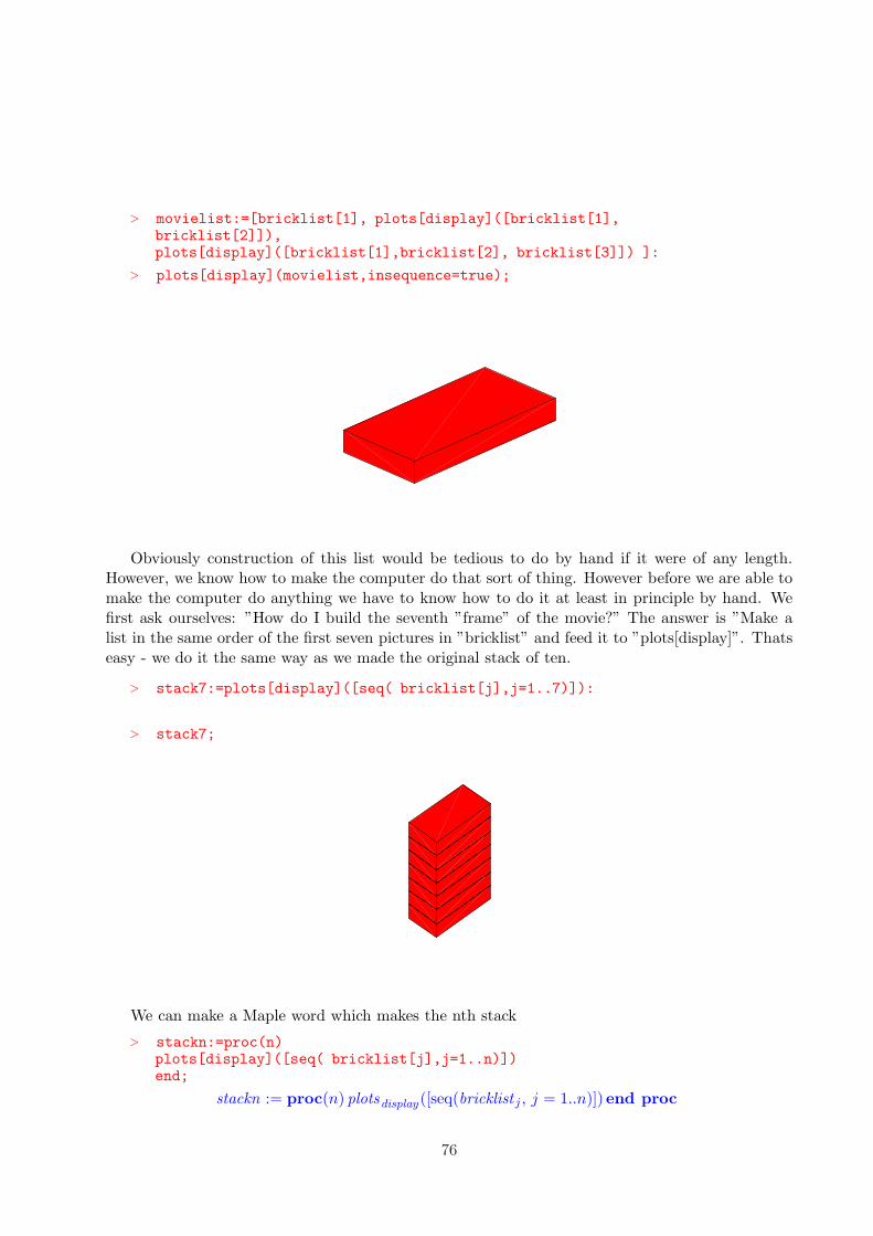
> movielist:=[bricklist[1], plots[display]([bricklist[1],bricklist[2]]),plots[display]([bricklist[1],bricklist[2], bricklist[3]]) ]:

> plots[display](movielist,insequence=true);

Obviously construction of this list would be tedious to do by hand if it were of any length.However, we know how to make the computer do that sort of thing. However before we are able tomake the computer do anything we have to know how to do it at least in principle by hand. Wefirst ask ourselves: ”How do I build the seventh ”frame” of the movie?” The answer is ”Make alist in the same order of the first seven pictures in ”bricklist” and feed it to ”plots[display]”. Thatseasy - we do it the same way as we made the original stack of ten.

> stack7:=plots[display]([seq( bricklist[j],j=1..7)]):

> stack7;

We can make a Maple word which makes the nth stack

> stackn:=proc(n)plots[display]([seq( bricklist[j],j=1..n)])end;

stackn := proc(n) plotsdisplay ([seq(bricklist j , j = 1..n)]) end proc

76

> stackn(3);

Now we can easily make our movie

> movie:=[seq(stackn(t),t=1..10)]:

> movie:=[op(movie),seq(movie[11-i],i=1..10)]:


In the previous example we were dealing with an extant list of known length. What if we didn’tknow the length of ”bricklist”. We might ask Maple to display it by entering its name and try tocount the entries. However it might be very long with each entry very complicated. There is asimple solution

If ”L” is a list then nops (L); returns the length of ”L”.> nops(bricklist);

10

> nops(movie);

77

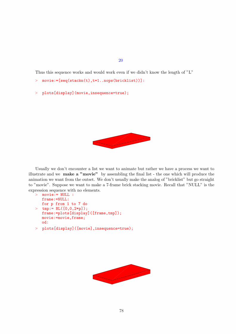
20

Thus this sequence works and would work even if we didn’t know the length of ”L”

> movie:=[seq(stackn(t),t=1..nops(bricklist))]:


Usually we don’t encounter a list we want to animate but rather we have a process we want toillustrate and we make a ”movie” by assembling the final list - the one which will produce theanimation we want from the outset. We don’t usually make the analog of ”bricklist” but go straightto ”movie”. Suppose we want to make a 7-frame brick stacking movie. Recall that ”NULL” is theexpression sequence with no elements.

> movie:= NULL :frame:=NULL:for p from 1 to 7 do

> tmp:= BL([0,0,2*p]);frame:=plots[display]([frame,tmp]);movie:=movie,frame;od:


78

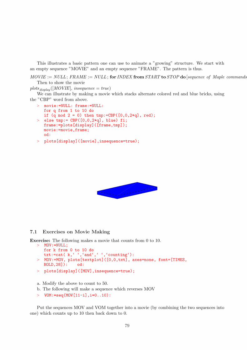
This illustrates a basic pattern one can use to animate a ”growing” structure. We start withan empty sequence ”MOVIE” and an empty sequence ”FRAME”. The pattern is thus.

MOVIE := NULL ; FRAME := NULL ; for INDEX fromSTART toSTOP do [sequence of Maple commandsThen to show the movie

plotsdisplay ([MOVIE ], insequence = true)We can illustrate by making a movie which stacks alternate colored red and blue bricks, using

the ”CBP” word from above.

> movie:=NULL: frame:=NULL:for q from 1 to 10 doif (q mod 2 = 0) then tmp:=CBP([0,0,2*q], red);

> else tmp:= CBP([0,0,2*q], blue) fi;frame:=plots[display]([frame,tmp]);movie:=movie,frame;od:


7.1 Exercises on Movie Making

Exercise: The following makes a movie that counts from 0 to 10.> MOV:=NULL;

for k from 0 to 10 dotxt:=cat( k,‘ ‘,‘and‘,‘ ‘,‘counting‘):

> MOV:=MOV, plots[textplot]([0,0,txt], axes=none, font=[TIMES,BOLD,28]): od:

> plots[display]([MOV],insequence=true);

a. Modify the above to count to 50.b. The following will make a sequence which reverses MOV

> VOM:=seq(MOV[11-i],i=0..10):

Put the sequences MOV and VOM together into a movie (by combining the two sequences intoone) which counts up to 10 then back down to 0.

79

c, Make a movie that counts from 3 to 9 then down to -5.

Exercise (Movie Splicing):a. Modify the following movie from the chapter text to make 10 frame movie of bricks stacking.

Call it ”tenbricks”.

> sevenbricks:= NULL ;frame:=NULL;for p from 1 to 7 do

> tmp:= BL([0,0,2*p]);frame:=plots[display]([frame,tmp]);sevenbricks:=sevenbricks,frame;od:


b. Make a movie called ”OnetoTen” which counts from 1 to to by making a sequence of all butthe first frame of the movie ”MOV” in the previous problem.

c. Splice the two movies together by making a 10-frame sequence ”MergedMovie” in which theith element is plots[display[(MOV[i], OnetoTen[i]);

d. When ”MergedMovie” is played the text meets the bricks. Look at the code for ”MOV” anddetermine the computer is being told to place the text. Modify the location of the text so that itsits below the brick stack with the stack approximately over the center of the text.

Exercise: As in the chapter text the following makes a movie of alternate red, white, and bluebricks stacking.

> movie:=NULL: frame:=NULL:for q from 1 to 10 doif (q mod 2 = 0) then tmp:=CBP([0,0,2*q], red);

> else tmp:= CBP([0,0,2*q], blue) fi;frame:=plots[display]([frame,tmp]);movie:=movie,frame;od:

If one selects the ’continuous’ option in the animation menu the movie will cycle when you playit. The motion is not smooth however, because the movie is played from beginning to end over andover. One would like to have the bricks stack up and then ”unstack”. Do this by making a moviewhich is twice as long as this one, having the bricks unstack in the last half of the movie so thatwhen you play it continuously, the motion is smooth. this can be done without making any moreimages.

Exercise: Make the hopping brick hop along a yellow road. Let each hop cover one bricklength with three frames of the brick ”in the air” beween frames in which it is ”on the road”.

Exercise: Make the brick move end over end along a yellow road.Exercise: Make a pair of bricks, a blue one and a red one move in a straight line with each

one ”leap frogging” the other.

80

8 New Problems from Old-A Case Study

One of the best ways to develop new problem contexts is to take old, familiar problems and lookat them in new ways. Developing alternate perspectives is as much art as science. However thereare some general techniques. One of the simplest is taking an old war horse of a problem andproducing a visual representation it and/or its solution. One almost always finds that this leads tonew, interesting problems. Here is an example:

8.1 The lawn mowing problem

Problem: Sam can mow the lawn in 2 hours and Bill can mow it in 3. How fast can they mow ittogether?

Solution: The problem implicitly assumes that Sam and Bill can work independently. When

this holds their rates add. Sam can mow one lawn in 2 hours so his rate is 1 lawn2 hours = 1

2 lawn per

hour. Similarly Bill has a rate of 13 lawn per hour. Together their rate is 1

2 + 13 = 5

6 lawn per hour

so together they can mow one lawn in 56 hour. Similar problems with essentially the same solution

can be stated for such things as two pipes filling a tank, two boys eating a pizza, etc. and of coursethe extension to more than two is no problem, with the assumption of independence of action anynumber of rates add. Traditional extensions don’t go much further than considering more than twomowers, pipes, etc.

8.2 Visual problems arising from the lawn mowing problem.

There any number of ways in which we might create a visual representation of this problem. Wecould do something as simple as making three bricks whose lengths represent the time Sam, Bill,and the two together could mow the lawn. This would be a straightforward application of what wehave already done but it wouldn’t be very interesting. For instance, it would not reflect the visualimage engendered by the original question. It would apply equally well to two pipes that couldindividually drain a tank in 2 and 3 hours. Moreover a static image would not convey the sense oftime or the feeling of motion conveyed by the mowing of a lawn.

Let us start by trying to convey the notion of one individual mowing one lawn

Although our work has been in three dimensions up to now the two dimensional case of thisproblem is simpler and less consumptive of computing resources so we start there.

First we need a lawn:

> v1:=[0,0]: v2:=[1,0]:v3:=[1,1]: v4:=[0,1]:lawn:=[v1,v2,v3,v4]:

> plots[polygonplot ](lawn,color=green, style=patch);

81

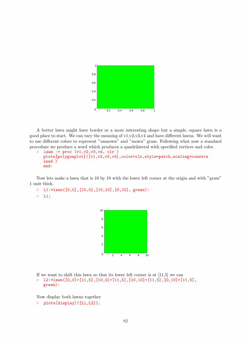
0

0.2

0.4

0.6

0.8

1

0.2 0.4 0.6 0.8 1

A better lawn might have border or a more interesting shape but a simple, square lawn is agood place to start. We can vary the meaning of v1,v2,v3,v4 and have different lawns. We will wantto use different colors to represent ”unmown” and ”mown” grass. Following what now a standardprocedure we produce a word which produces a quadrilateral with specified vertices and color.

> lawn := proc (v1,v2,v3,v4, clr )plots[polygonplot]([v1,v2,v3,v4],color=clr,style=patch,scaling=constrained )end:

Now lets make a lawn that is 10 by 10 with the lower left corner at the origin and with ”grass”1 unit thick.

> L1:=lawn([0,0],[10,0],[10,10],[0,10], green):

> L1;

0

2

4

6

8

10

2 4 6 8 10

If we want to shift this lawn so that its lower left corner is at [11,5] we can> L2:=lawn([0,0]+[11,5],[10,0]+[11,5],[10,10]+[11,5],[0,10]+[11,5],

green):

Now display both lawns together> plots[display]([L1,L2]);

82

0

2

4

6

8

10

12

14

5 10 15 20

If we decide that ”unmown” grass is aquamarine and ”mown” grass is green then we can indicatea partially mown lawn by laying a ”mown” green plot on top of an ”unmown” aquamarine one.We could just as easily have adjoining plots of different colors but our there will be less calculatingfurther on if we do it this way.

> L1:=lawn([0,0],[10,0],[10,10],[0,10], aquamarine):L2:=lawn([0,0] ,[4,0] ,[4,4] ,[0,4] , green):plots[display]([L2,L1]);

0

2

4

6

8

10

2 4 6 8 10

Note in the plots[display]([L2,L1]) the ”L2,L1” order. This tells the computer to lay L1 downfirst and L2 on top of it. If we do things in the opposite order there will be a difference. Changethe order and note the difference.

Now we have all we need to animate mowing a lawn - all we need to do is successively enlargethe ”mown” portion until it covers the lawn. We ”mow” it a strip at a time, combining the stripswe have done into a single rectangle. First lets mow a strip.

Suppose, we have a strip which is 2 units wide and 30 long and wish to animate mowing it witha lawnmower 2 units wide over the course of 10 units of time. We can draw this sketch. Letting”t” vary from 0 to 10 we note that the middle line in our sketch varies from the left edge to theright of the larger rectangle. Thinking of this as the boundary of our mown and unmown grass wecan, for any value of t between 0 and 10 delineate the two.

83

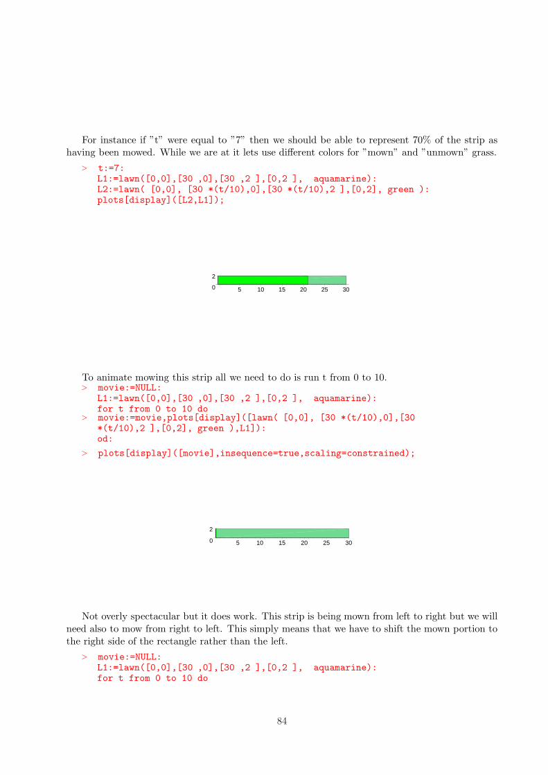
For instance if ”t” were equal to ”7” then we should be able to represent 70% of the strip ashaving been mowed. While we are at it lets use different colors for ”mown” and ”unmown” grass.

> t:=7:L1:=lawn([0,0],[30 ,0],[30 ,2 ],[0,2 ], aquamarine):L2:=lawn( [0,0], [30 *(t/10),0],[30 *(t/10),2 ],[0,2], green ):plots[display]([L2,L1]);

0

2

5 10 15 20 25 30

To animate mowing this strip all we need to do is run t from 0 to 10.> movie:=NULL:

L1:=lawn([0,0],[30 ,0],[30 ,2 ],[0,2 ], aquamarine):for t from 0 to 10 do

> movie:=movie,plots[display]([lawn( [0,0], [30 *(t/10),0],[30*(t/10),2 ],[0,2], green ),L1]):od:

> plots[display]([movie],insequence=true,scaling=constrained);

0

2

5 10 15 20 25 30

Not overly spectacular but it does work. This strip is being mown from left to right but we willneed also to mow from right to left. This simply means that we have to shift the mown portion tothe right side of the rectangle rather than the left.

> movie:=NULL:L1:=lawn([0,0],[30 ,0],[30 ,2 ],[0,2 ], aquamarine):for t from 0 to 10 do

84

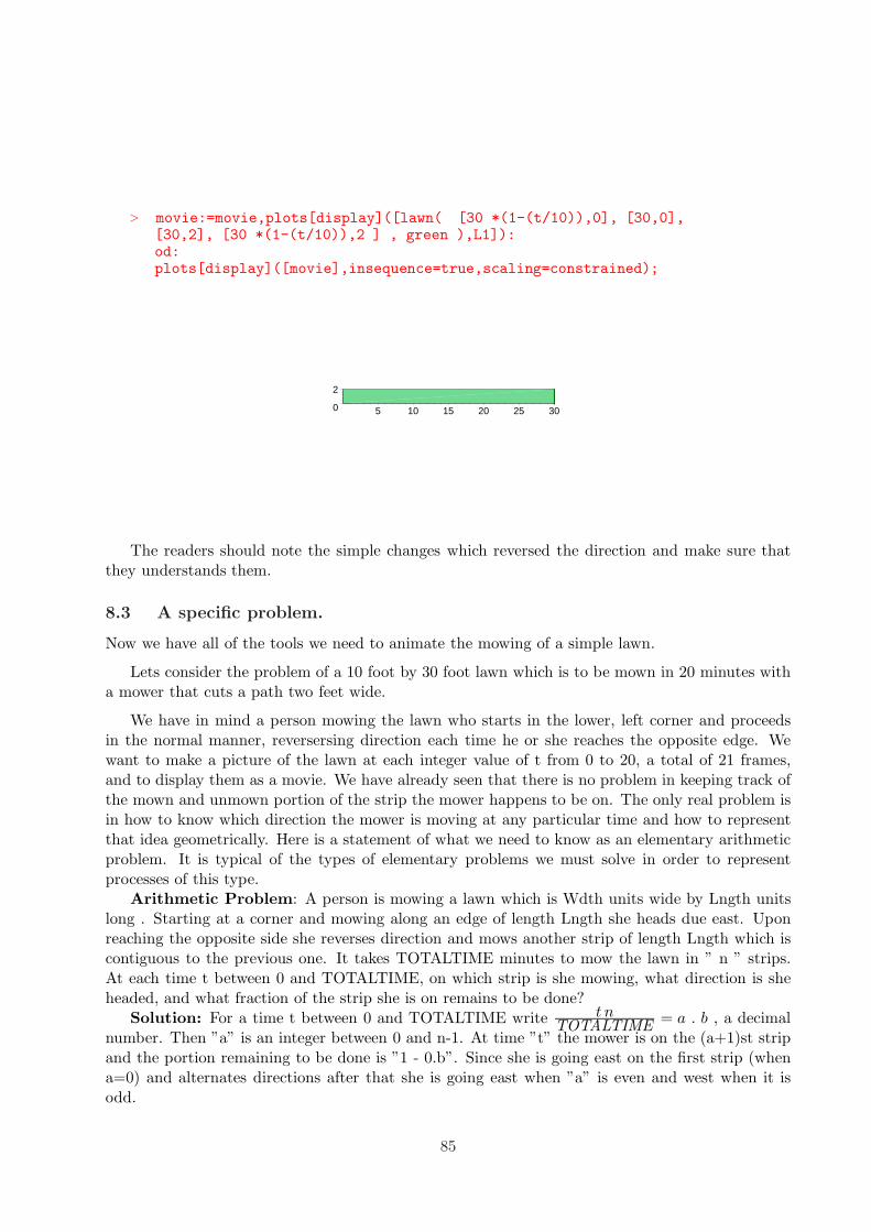
> movie:=movie,plots[display]([lawn( [30 *(1-(t/10)),0], [30,0],[30,2], [30 *(1-(t/10)),2 ] , green ),L1]):od:plots[display]([movie],insequence=true,scaling=constrained);

0

2

5 10 15 20 25 30

The readers should note the simple changes which reversed the direction and make sure thatthey understands them.

8.3 A specific problem.

Now we have all of the tools we need to animate the mowing of a simple lawn.

Lets consider the problem of a 10 foot by 30 foot lawn which is to be mown in 20 minutes witha mower that cuts a path two feet wide.

We have in mind a person mowing the lawn who starts in the lower, left corner and proceedsin the normal manner, reversersing direction each time he or she reaches the opposite edge. Wewant to make a picture of the lawn at each integer value of t from 0 to 20, a total of 21 frames,and to display them as a movie. We have already seen that there is no problem in keeping track ofthe mown and unmown portion of the strip the mower happens to be on. The only real problem isin how to know which direction the mower is moving at any particular time and how to representthat idea geometrically. Here is a statement of what we need to know as an elementary arithmeticproblem. It is typical of the types of elementary problems we must solve in order to representprocesses of this type.

Arithmetic Problem: A person is mowing a lawn which is Wdth units wide by Lngth unitslong . Starting at a corner and mowing along an edge of length Lngth she heads due east. Uponreaching the opposite side she reverses direction and mows another strip of length Lngth which iscontiguous to the previous one. It takes TOTALTIME minutes to mow the lawn in ” n ” strips.At each time t between 0 and TOTALTIME, on which strip is she mowing, what direction is sheheaded, and what fraction of the strip she is on remains to be done?

Solution: For a time t between 0 and TOTALTIME write t nTOTALTIME = a . b , a decimal

number. Then ”a” is an integer between 0 and n-1. At time ”t” the mower is on the (a+1)st stripand the portion remaining to be done is ”1 - 0.b”. Since she is going east on the first strip (whena=0) and alternates directions after that she is going east when ”a” is even and west when it isodd.

85

The Maple command for the integer part of a number, the greatest integer function, is calledfloor.

The remainder of an integer ”m” upon division by two is m mod 2

> floor(3.2);floor(3.2) mod 2;

3

1

With the notation of the Arithmetic Problem our original problem has Wdth=10, Lngth=30,n=5, TOTALTIME=20. Ultimately we will make a 21 frame animation but the cardinal rule isalways develop an individual frame first. We start with, say, t=9. then for this frame

> t:=9; n:=5; TOTALTIME:=20;Wdth:=10; Lngth:=30;a:= floor(t*n/TOTALTIME);b:=t*n/TOTALTIME - a;a;

t := 9

n := 5

TOTALTIME := 20

Wdth := 10

Lngth := 30

a := 2

b :=1

42

This tells us that the third strip is being mown, moving east (since ”a” is even). One forth ofthe strip has been mown and 3/4 remains to be mown.

Now we can animate the lawn being mown. Each frame correesponds to a value of t from 0 toTOTALTIME. For the frame at time t we need to:

• 1. Calculate which strip we are mowing, the direction and what portion of the strip has beenmown.

• 2. Make a rectangle green MOWN consisting of all complete strips mown

• 3. Make a green rectangle STRIPMOWN consisting of the portion of the current strip thathas been mown then the frame is [STRIPMOWN, MOWN, UUNMOWN] where UNMOWNis the complete lawn colored aquamarine.

Here is a first try at the code

> TIME:=9: NUMSTRIPS:=5: TOTALTIME:=20:Wdth:=10: Lngth:=30:movie:=NULL:

86

> YARD:=lawn([0,0],[30 , 0],[30 ,10 ],[ 0,10 ],aquamarine):for TIME from 0 to TOTALTIME doWHICHSTRIP:= floor(NUMSTRIPS*TIME/TOTALTIME);

> FRACSTRIP:=TIME*(NUMSTRIPS/TOTALTIME) - WHICHSTRIP;MOWN:=lawn( [0,0],[30,0],[30,2*WHICHSTRIP],[0,2*WHICHSTRIP] , green):

> if WHICHSTRIP mod 2 = 0 thenFrame:=plots[display]([MOWN, lawn( [0,2*(WHICHSTRIP )] ,[30 *FRACSTRIP,2*(WHICHSTRIP )], [30*FRACSTRIP,

> 2*(WHICHSTRIP+1) ], [0,2*(WHICHSTRIP+1)], green ) ],YARD):elseFrame:=plots[display]([MOWN, lawn( [30 *(1-FRACSTRIP),

> 2*(WHICHSTRIP )], [30,2*(WHICHSTRIP )],[30,2*(WHICHSTRIP+1)], [30 *( 1- FRACSTRIP),2*(WHICHSTRIP+1) ] , green ) ],YARD):

> fi:movie:=movie,Frame:od:


0

2

4

6

8

10

12

5 10 15 20 25 30

This works pretty well but but we need to test it by varying the values of the parameters. Letscheck it with some new ones. As is our procedure we make another copy of the working code ratherthan tampering with it.

> NUMSTRIPS:=7: TOTALTIME:=25:Wdth:=37:Lngth:=30:> movie:=NULL:

YARD:=lawn([0,0],[30 , 0],[30 ,10 ],[ 0,10 ], aquamarine):for TIME from 0 to TOTALTIME do

> WHICHSTRIP:= floor(NUMSTRIPS*TIME/TOTALTIME);FRACSTRIP:=TIME*(NUMSTRIPS/TOTALTIME) - WHICHSTRIP;MOWN:=lawn( [0,0],[30,0],[30,2*WHICHSTRIP],

> [0,2*WHICHSTRIP] ,green): if WHICHSTRIP mod 2 = 0 thenFrame:=plots[display]([MOWN, lawn( [0,2*(WHICHSTRIP )] ,[30 *FRACSTRIP,2*(WHICHSTRIP ) ],

> [30*FRACSTRIP,2*(WHICHSTRIP+1) ],[0,2*(WHICHSTRIP+1)], green ) ],YARD):else

87

> Frame:=plots[display]([MOWN, lawn([30 *( 1-FRACSTRIP),2*(WHICHSTRIP )],[30,2*(WHICHSTRIP )], [30,2*(WHICHSTRIP+1)],

> [30 *( 1- FRACSTRIP),2*(WHICHSTRIP+1) ] , green ) ],YARD):fi:movie:=movie,Frame:od:


0

2

4

6

8

10

12

14

16

5 10 15 20 25 30

Hmmm.... little problem here. What happened caused it to work for one set of data and notfor another is that we had ”hard coded” some ”magic numbers”. One of them was ”2” the widthof the strip. We told the computer to mow a 37 foot wide lawn in 7 strips two foot wide strips.It got confused. We correct that by letting ir calculate the width of its mower as the ratio of thewidth of the lawn to the number of strips.

> movie:=NULL:YARD:=lawn([0,0],[30 , 0],[30 ,10 ],[ 0,10 ], aquamarine):MRWDTH:=Wdth/NUMSTRIPS:

> for TIME from 0 to TOTALTIME doWHICHSTRIP:= floor(NUMSTRIPS*TIME/TOTALTIME);FRACSTRIP:=TIME*(NUMSTRIPS/TOTALTIME) - WHICHSTRIP;

> MOWN:=lawn( [0,0],[30,0],[30,MRWDTH*WHICHSTRIP],[0,MRWDTH*WHICHSTRIP] ,green):if WHICHSTRIP mod 2 = 0 then

> Frame:=plots[display]([MOWN, lawn( [0,MRWDTH*(WHICHSTRIP )] ,[30 *FRACSTRIP,MRWDTH*(WHICHSTRIP )],[30*FRACSTRIP,MRWDTH*(WHICHSTRIP+1)],

> [0,MRWDTH*(WHICHSTRIP+1)], green ) ],YARD):elseFrame:=plots[display]([MOWN, lawn(

> [30 *( 1-FRACSTRIP),MRWDTH*(WHICHSTRIP )],[30,MRWDTH*(WHICHSTRIP )], [30,MRWDTH*(WHICHSTRIP+1)],[30 *( 1- FRACSTRIP),MRWDTH*(WHICHSTRIP+1) ] , green ) ], YARD):


88


0

10

20

30

40

5 10 15 20 25 30

Pretty close now - we forgot the other ”magic numbers” ”30” and ”10” in the code. They werethe length and width of our original lawn. All we have to do is substitute the variables ”Wdth”and ”Lngth” for them:

> movie:=NULL:YARD:=lawn([0,0],[Lngth , 0],[Lngth ,Wdth ],[ 0,Wdth ],aquamarine):

> MRWDTH:=Wdth/NUMSTRIPS:for TIME from 0 to TOTALTIME doWHICHSTRIP := floor(NUMSTRIPS*TIME/TOTALTIME);

> FRACSTRIP := TIME*(NUMSTRIPS/TOTALTIME) - WHICHSTRIP;MOWN := lawn( [0,0],[Lngth,0],[Lngth,MRWDTH*WHICHSTRIP],[0,MRWDTH*WHICHSTRIP] ,green):

> if WHICHSTRIP mod 2 = 0 thenFrame := plots[display]([MOWN, lawn([0,MRWDTH*(WHICHSTRIP )] ,

> [Lngth *FRACSTRIP,MRWDTH*(WHICHSTRIP )],[Lngth*FRACSTRIP,MRWDTH*(WHICHSTRIP+1)],[0,MRWDTH*(WHICHSTRIP+1)], green ) ],YARD):

> elseFrame := plots[display]([MOWN, lawn([Lngth *( 1-FRACSTRIP),MRWDTH*(WHICHSTRIP )],

> [Lngth,MRWDTH*(WHICHSTRIP )],[Lngth,MRWDTH*(WHICHSTRIP+1)],[Lngth *( 1- FRACSTRIP),MRWDTH*(WHICHSTRIP+1) ] ,

> green ) ],YARD):fi:movie:=movie,Frame:od:


89

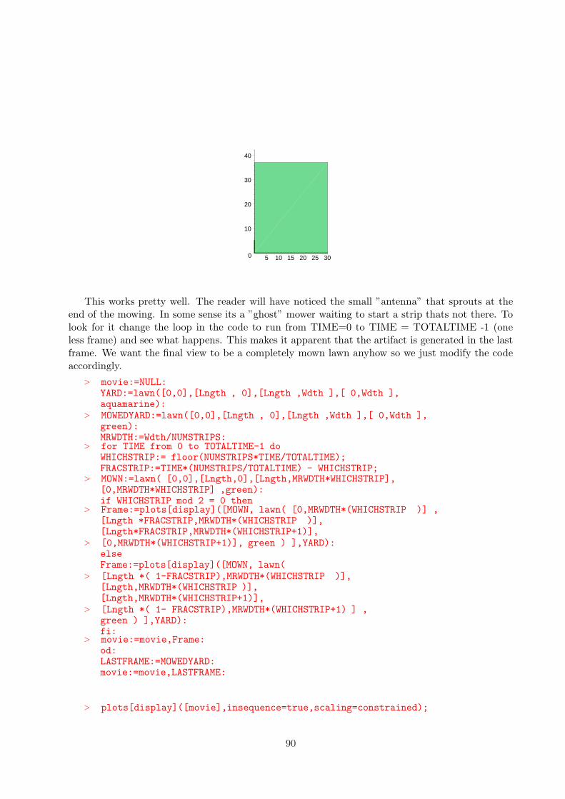
0

10

20

30

40

5 10 15 20 25 30

This works pretty well. The reader will have noticed the small ”antenna” that sprouts at theend of the mowing. In some sense its a ”ghost” mower waiting to start a strip thats not there. Tolook for it change the loop in the code to run from TIME=0 to TIME = TOTALTIME -1 (oneless frame) and see what happens. This makes it apparent that the artifact is generated in the lastframe. We want the final view to be a completely mown lawn anyhow so we just modify the codeaccordingly.


> MOWEDYARD:=lawn([0,0],[Lngth , 0],[Lngth ,Wdth ],[ 0,Wdth ],green):MRWDTH:=Wdth/NUMSTRIPS:

> for TIME from 0 to TOTALTIME-1 doWHICHSTRIP:= floor(NUMSTRIPS*TIME/TOTALTIME);FRACSTRIP:=TIME*(NUMSTRIPS/TOTALTIME) - WHICHSTRIP;

> MOWN:=lawn( [0,0],[Lngth,0],[Lngth,MRWDTH*WHICHSTRIP],[0,MRWDTH*WHICHSTRIP] ,green):if WHICHSTRIP mod 2 = 0 then

> Frame:=plots[display]([MOWN, lawn( [0,MRWDTH*(WHICHSTRIP )] ,[Lngth *FRACSTRIP,MRWDTH*(WHICHSTRIP )],[Lngth*FRACSTRIP,MRWDTH*(WHICHSTRIP+1)],

> [0,MRWDTH*(WHICHSTRIP+1)], green ) ],YARD):elseFrame:=plots[display]([MOWN, lawn(

> [Lngth *( 1-FRACSTRIP),MRWDTH*(WHICHSTRIP )],[Lngth,MRWDTH*(WHICHSTRIP )],[Lngth,MRWDTH*(WHICHSTRIP+1)],

> [Lngth *( 1- FRACSTRIP),MRWDTH*(WHICHSTRIP+1) ] ,green ) ],YARD):fi:

> movie:=movie,Frame:od:LASTFRAME:=MOWEDYARD:movie:=movie,LASTFRAME:


90

0

5

10

15

20

25

30

35

5 10 15 20 25 30

8.3.1 A lawn mowing word

Finally, we make this into a procedure which accepts the dimensions of a lawn, the number ofstrips, and the total time it takes to mow it (i.e. the number of frames in the movie) and returnsa movie of that lawm being mowed in that time.

> lawnmower:=proc(Lngth, Wdth, TOTALTIME, NUMSTRIPS)local movie, YARD, MOWEDYARD, MRWDTH, TIME, WHICHSTRIP, FRACSTRIP,MOWN, Frame, LASTFRAME;

> Digits :=4:movie:=NULL:YARD:=lawn([0,0],[Lngth , 0],[Lngth ,Wdth ],[ 0,Wdth ],

> aquamarine):MOWEDYARD:=lawn([0,0],[Lngth , 0],[Lngth ,Wdth ],[ 0,Wdth ],green):

> MRWDTH:=Wdth/NUMSTRIPS:for TIME from 0 to TOTALTIME-1 doWHICHSTRIP:= floor(NUMSTRIPS*TIME/TOTALTIME);

> FRACSTRIP:=TIME*(NUMSTRIPS/TOTALTIME) - WHICHSTRIP;MOWN:=lawn( [0,0],[Lngth,0],[Lngth,MRWDTH*WHICHSTRIP],[0,MRWDTH*WHICHSTRIP] ,green):

> if WHICHSTRIP mod 2 = 0 thenFrame:=plots[display]([MOWN, lawn( [0,MRWDTH*(WHICHSTRIP )] ,[Lngth *FRACSTRIP,MRWDTH*(WHICHSTRIP )],

> [Lngth*FRACSTRIP,MRWDTH*(WHICHSTRIP+1)],[0,MRWDTH*(WHICHSTRIP+1)], green ) ],YARD):else

> Frame:=plots[display]([MOWN, lawn([Lngth *( 1-FRACSTRIP),MRWDTH*(WHICHSTRIP )],[Lngth,MRWDTH*(WHICHSTRIP )],

> [Lngth,MRWDTH*(WHICHSTRIP+1)],[Lngth *( 1- FRACSTRIP),MRWDTH*(WHICHSTRIP+1) ] ,green ) ],YARD):


91

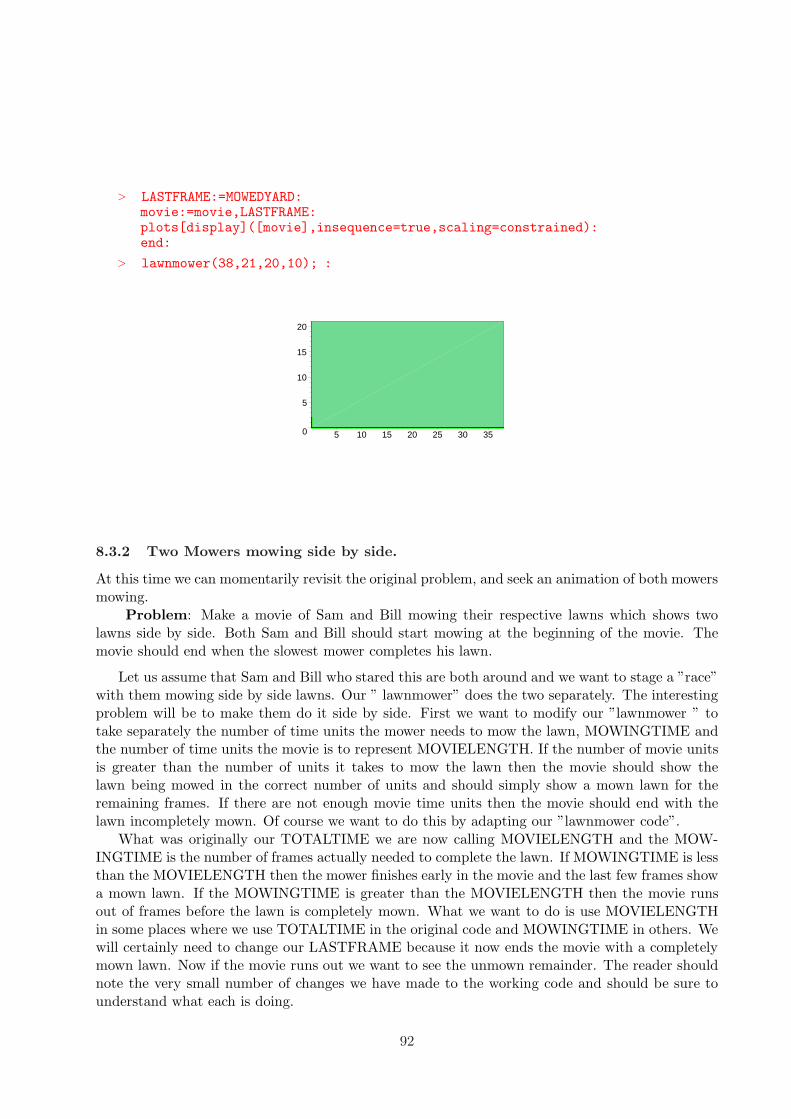
> LASTFRAME:=MOWEDYARD:movie:=movie,LASTFRAME:plots[display]([movie],insequence=true,scaling=constrained):end:

> lawnmower(38,21,20,10); :

0

5

10

15

20

5 10 15 20 25 30 35

8.3.2 Two Mowers mowing side by side.

At this time we can momentarily revisit the original problem, and seek an animation of both mowersmowing.

Problem: Make a movie of Sam and Bill mowing their respective lawns which shows twolawns side by side. Both Sam and Bill should start mowing at the beginning of the movie. Themovie should end when the slowest mower completes his lawn.

Let us assume that Sam and Bill who stared this are both around and we want to stage a ”race”with them mowing side by side lawns. Our ” lawnmower” does the two separately. The interestingproblem will be to make them do it side by side. First we want to modify our ”lawnmower ” totake separately the number of time units the mower needs to mow the lawn, MOWINGTIME andthe number of time units the movie is to represent MOVIELENGTH. If the number of movie unitsis greater than the number of units it takes to mow the lawn then the movie should show thelawn being mowed in the correct number of units and should simply show a mown lawn for theremaining frames. If there are not enough movie time units then the movie should end with thelawn incompletely mown. Of course we want to do this by adapting our ”lawnmower code”.

What was originally our TOTALTIME we are now calling MOVIELENGTH and the MOW-INGTIME is the number of frames actually needed to complete the lawn. If MOWINGTIME is lessthan the MOVIELENGTH then the mower finishes early in the movie and the last few frames showa mown lawn. If the MOWINGTIME is greater than the MOVIELENGTH then the movie runsout of frames before the lawn is completely mown. What we want to do is use MOVIELENGTHin some places where we use TOTALTIME in the original code and MOWINGTIME in others. Wewill certainly need to change our LASTFRAME because it now ends the movie with a completelymown lawn. Now if the movie runs out we want to see the unmown remainder. The reader shouldnote the very small number of changes we have made to the working code and should be sure tounderstand what each is doing.

92

> lawnmower2:=proc(Lngth, Wdth, MOWINGTIME, MOVIELENGTH, NUMSTRIPS)local movie, YARD, MOWEDYARD, MRWDTH, TIME, WHICHSTRIP, FRACSTRIP,MOWN, Frame, LASTFRAME;


> MOWEDYARD:=lawn([0,0],[Lngth , 0],[Lngth ,Wdth ],[ 0,Wdth ],green):MRWDTH:=Wdth/NUMSTRIPS:

> for TIME from 0 to MOVIELENGTH-1 doif TIME <=MOWINGTIME thenWHICHSTRIP:= floor(NUMSTRIPS*TIME/MOWINGTIME);

> FRACSTRIP:=TIME*(NUMSTRIPS/MOWINGTIME) - WHICHSTRIP;MOWN:=lawn([ 0,0],[Lngth,0],[Lngth,MRWDTH*WHICHSTRIP],[0,MRWDTH*WHICHSTRIP] ,green):

> if WHICHSTRIP mod 2 = 0 thenFrame:=plots[display]([MOWN, lawn( [0,MRWDTH*(WHICHSTRIP )] ,[Lngth *FRACSTRIP,MRWDTH*(WHICHSTRIP )],

> [Lngth*FRACSTRIP,MRWDTH*(WHICHSTRIP+1) ], [0,MRWDTH*(WHICHSTRIP+1)],green ) ],YARD):else

> Frame:=plots[display]([MOWN, lawn([Lngth *( 1-FRACSTRIP),MRWDTH*(WHICHSTRIP )],[Lngth,MRWDTH*(WHICHSTRIP )],

> [Lngth,MRWDTH*(WHICHSTRIP+1)],[Lngth *( 1- FRACSTRIP),MRWDTH*(WHICHSTRIP+1) ] ,green ) ],YARD):

> fi:movie:=movie,Frame:else

> movie:=movie,MOWEDYARD:fi:od:

> if MOVIELENGTH >= MOWINGTIME then LASTFRAME:=MOWEDYARD:movie:=movie,LASTFRAME:plots[display]([movie],insequence=true,scaling=constrained):

> fi:end:

> lawnmower2(30,20,7,20,10);

0

5

10

15

20

5 10 15 20 25 30

93

Now if we want side-by-side mowers we need different lawns. This we need to introduce a shiftwhich moves the original lawn to a different location. BEFORE we start directly into this howeverwe examine what we have done and notice that the only way that coordinates are used is in theword ”lawn”. Thus if we simply adapt the word ”lawn” to accept a shift (it probably should havehad one anyhow). We are also changing our porgram so that it returns the movie rather than playsit. This is because we are going to want to run two movies at the same time so we will need to”splice” them together.

> lawnwithshift := proc (v1,v2,v3,v4, clr, shift)plots[polygonplot]([v1+shift,v2+shift,v3+shift,v4+shift],color=clr,style=patch,scaling=constrained ) end:

> lawnmower3:=proc(Lngth, Wdth, MOWINGTIME, MOVIELENGTH,NUMSTRIPS,SHIFT)local movie, YARD, MOWEDYARD, MRWDTH, TIME, WHICHSTRIP,

> FRACSTRIP, MOWN, Frame, LASTFRAME;movie:=NULL:YARD:=lawnwithshift([0,0],[Lngth , 0],[Lngth ,Wdth ],[ 0,Wdth ],

> aquamarine,SHIFT):MOWEDYARD:=lawnwithshift([0,0],[Lngth , 0],[Lngth ,Wdth ],[ 0,Wdth],

> green,SHIFT):MRWDTH:=Wdth/NUMSTRIPS:for TIME from 0 to MOVIELENGTH-1 do

> if TIME <=MOWINGTIME thenWHICHSTRIP:= floor(NUMSTRIPS*TIME/MOWINGTIME);FRACSTRIP:=TIME*(NUMSTRIPS/MOWINGTIME) - WHICHSTRIP;

> MOWN:=lawnwithshift([0,0],[Lngth,0],[Lngth,MRWDTH*WHICHSTRIP],[0,MRWDTH*WHICHSTRIP] ,green,SHIFT):

> if WHICHSTRIP mod 2 = 0 thenFrame:=plots[display]([MOWN, lawnwithshift( [0,MRWDTH*(WHICHSTRIP)] ,

> [Lngth *FRACSTRIP,MRWDTH*(WHICHSTRIP )],[Lngth*FRACSTRIP,MRWDTH*(WHICHSTRIP+1) ],[0,MRWDTH*(WHICHSTRIP+1)], green,SHIFT ) ],YARD):

> elseFrame:=plots[display]([MOWN, lawnwithshift([Lngth *( 1-FRACSTRIP),MRWDTH*(WHICHSTRIP )],

> [Lngth,MRWDTH*(WHICHSTRIP )],[Lngth,MRWDTH*(WHICHSTRIP+1)],[Lngth *( 1- FRACSTRIP),MRWDTH*(WHICHSTRIP+1) ] ,

> green,SHIFT ) ],YARD):fi:movie:=movie,Frame:

> elsemovie:=movie,MOWEDYARD:fi:

94

> od:if MOVIELENGTH >= MOWINGTIME thenLASTFRAME:=MOWEDYARD:

> movie:=movie,LASTFRAME:plots[display]([movie],insequence=true):fi:[movie];end:

> MOVIE:=lawnmower3(30,20,13,20,10,[32,0]):plots[display]( MOVIE,insequence=true);

0

5

10

15

20

35 40 45 50 55 60

Now lets assume that Sam and Bill are next door neighbors with idential 20 by 30 lawns. Theyeach have a lawnmower which will mow their lawn in 7 strips. Sam can mow his lawn in 15 timeunits and Bill can mow his in 30. We can view each of them mowing his lawn with what we have:

> SAMMOWING:=lawnmower3(30,20,15,15,7,[0,0]):plots[display](SAMMOWING,insequence=true):

> BILLMOWING:=lawnmower3(30,20,30,30,7,[32,0]):plots[display](BILLMOWING,insequence=true);

0

2

4

6

8

10

12

14

16

18

20

35 40 45 50 55 60

If we are going to watch both of them we want to run the movie for the length of time it takesthe slowest person to do the job. Thus we need to make Sam’s movie run 30 units.

95

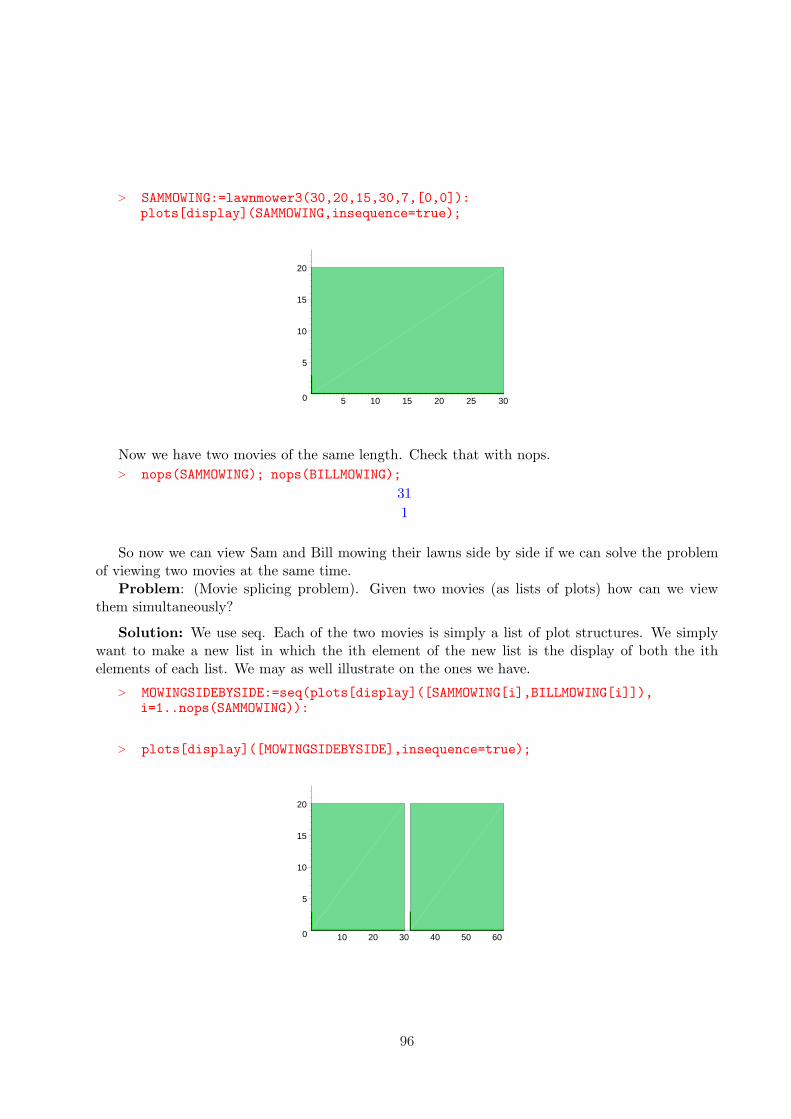
> SAMMOWING:=lawnmower3(30,20,15,30,7,[0,0]):plots[display](SAMMOWING,insequence=true);

0

5

10

15

20

5 10 15 20 25 30

Now we have two movies of the same length. Check that with nops.> nops(SAMMOWING); nops(BILLMOWING);

31

1

So now we can view Sam and Bill mowing their lawns side by side if we can solve the problemof viewing two movies at the same time.

Problem: (Movie splicing problem). Given two movies (as lists of plots) how can we viewthem simultaneously?

Solution: We use seq. Each of the two movies is simply a list of plot structures. We simplywant to make a new list in which the ith element of the new list is the display of both the ithelements of each list. We may as well illustrate on the ones we have.

> MOWINGSIDEBYSIDE:=seq(plots[display]([SAMMOWING[i],BILLMOWING[i]]),i=1..nops(SAMMOWING)):

> plots[display]([MOWINGSIDEBYSIDE],insequence=true);

0

5

10

15

20

10 20 30 40 50 60

96

8.3.3 Exercises

Exercise: Suppose A and B are rectangular tanks with identical dimensions, only B is below Aand rotated 90 degrees. At a certain time A is full and B is empty, then the valve between them isopened and all the fluid flows into B at a constant rate determined by the valve. Make a 20 framemovie showing the fluid level in each tank with A full at the beginning and B full at the end.

Beginning of Solution:

We aren’t given the dimensions of the tanks so we will assume some. The spacing isn’t giveneither, nor the orientations. In this case its our job to make some reasonable assumptions. This isbasically a two dimensional problem so we will let the tanks be one unit thick. The side view wouldlook the same regardless of how thick they were. Here is a diagram: There isn’t any mathematicaldifference between the description of a ”lawn” and the lateral view of a tank so we use our lawnprocedure.

> lawn := proc (v1,v2,v3,v4, clr )plots[polygonplot]([v1,v2,v3,v4],color=clr,style=patch,scaling=constrained ) end:

Our time is to run from t=0 to t=19 (20 frames) so at time t in this range tank B is t/19 fullwhile tank A is (1-t/19) full. This means that at time t between 0 and 19 the fluid level of tank Bis at 10*t/19 and that at tank A is at 37-25*t/19. Thus the fluid in tank A is described by

lawn([0,0],[25,0], [25,10*t/19],[0,10*t/19], red);

and that in tank B is described by

lawn([15,12],[25,12], [25,37-25*t/19],[15,37-25*t/19], red);A first approximation to our basic movie is:

> movie:=NULL: for t from 0 to 19 doframe:= plots[display]([ lawn([0,0],[25,0], [25,10*t/19],[0,10*t/19],red), lawn([15,12],[25,12], [25,37-25*t/19],[15,37-25*t/19], red)]

> ):movie:=movie,frame: od:


a. Modify the basic movie so that the complete tanks are there - not just the fluid.

b. Modify the movie so that the color of the fluid changes as if moves from tank A to tank B.

c. Add the pipe connecting the two tanks to the movie. Have the pipe full thorugh the last(t=19) frame of the current movie then add a new last frame (t=20) in which the pipe is empty.

Exercise: Suppose there are three tanks A,B,C arranged C on top and connected to each of Aand B. The volumes of tanks A and B are equal to that of tank C. When tank A is empty and Cis full and the valve between A and C is open then tank A will fill in 20 minutes. When tank B isempty and C is full and the valve between B and C is open then tank B will fill in 35 minutes. If

97

both tanks A and B are empty and tank full is empty, how long will it take for tank C to emptyand how much will be in each of tanks A and B at that time? Animate your answer.

Exercise: Suppose there are three tanks A,B,C arranged as in the preceding exercise. Thevolumes of tanks A and B are equal to half that of tank C. When tank A is empty and C is fulland the valve between A and C is open then tank A will fill in 20 minutes. When tank B is emptyand C is full and the valve between B and C is open then tank B will fill in 35 minutes. If bothtanks A and B are empty and tank full is empty, how long will it take for both tanks A and B tofill up? Animate your answer.

Exercise: Suppose there are three tanks A,B,C with A and B side by side on top of C. Asbefore A and B are each connected to C with a drain. The volumes of tanks A and B are equal tohalf that of tank C. When tank A is full and tanks A and C are empty all of the fluid in tank Awill flow into tank C in 20 minutes. When tank B is full and tanks A and C are empty all of thefluid in tank B will flow into tank C in 35 minutes. If both tanks A and B are full and tank C isempty, how long will it take for tanks A and B to fill tank C? Animate your answer.

Exercise: Modify the lawnmower code to accept the dimensions of the lawn and the width ifthe mower rather than the number of strips. Have it then calculate the number of strips and haveit deal rationally with what happens if the number of strips is not a whole number. This should bea reasonable thing for a real person to do when mowing such a lawn.

Exercise: Suppose Larry, Curley, and Moe are neighbors with identical 10 by 10 square lawns.It takes Larry 20 minutes to mow his lawn, Curley takes 15, and Moe 10. Make a movie of all threemowing their lawns, starting at the same time.

98

9 Mowing Yards (part 2)

9.1 Starting at Different Corners: Going in Different Directions

Up until now all of our mowing starts in the lower left corner of a square or rectangular lawn.Maybe we would like to start in the upper left and move in either direction, or even in the upperright. One way to do this would be to re-do all we have done before, only making everything startat some other point. That would involve repeating a considerable amount of effort when we knowintuitively that these problems and their solutions are all essentially equivalent. ”Lower left corner”obviously has no intrinsic meaning to a square. By rotating it any point could be ”lower” and byturning it over or looking at its reflection in a mirror the notions of ”left” and ”right” are reversed.By geometrically (visually) applying these ”symmetries” of the square we realize that the analysisof starting at any particular corner and heading in either possible direction can be described interms of what happens in the case we have already done. What we need to do is understand how toquantify the symmetries of the problem mathematically and apply the corresponding mathematicalsymmetries to the work we have already done.

For instance, what we did in the last was start mowing at the lower left corner. We could startat the lower right simply by reflecting everything through a line perpendicular to the x-axis whichbisects the yard. Suppose that we have arranged things so that the bisecting line is in fact they-axis.

Then the analytic (algebraic) realization of this reflection is simply reversing the sign of thex-coordinates. That is if P is the point [x,y] then the point which is the reflection of P through they-axis is simply [ -x,y]. What this means is that we can convert the algebra of mowing from left toright to that of mowing from right to left simply by changing some signs. This promises to be farmore simple that re-doing all of our previous work.

Of course in general the y-axis isn’t a line of symmetry of a problem but our powerful idea ofsymmetry tells us how to handle this: if there is a line of symmetry then since we can intuitivelysee that that all lines in the plane are ”equivalent” we can take the alebra which expersses theequivalence of the given line and the y-axis and use it to convert the analysis of the simple caseinto that of the one which interests us. For example, if the line of symmetry isn’t the y-axis butis parallel to it we can simply apply a shift which moves the line of symmetry to the y-axis, thenrefelect through the y-axis, then shift back. If the shift which moves our line to the y-axis is[SHIFTX, SHIFTY] then the recipe would simply be:

[ X, Y ] -> [ X + SHIFTX, Y + SHIFTY] -> [ -X - SHIFTX, Y + SHIFTY] -> [ -X -2* SHIFTX,Y ]

Applying this transformations to the vertices of a polygon (lawn) would then reflect that polygonthrough the given line. For instance if Larry’s lawn is Larryslawn:=[[0,0],[3,0],[3,1], [0,1]]; and wewant to refelect Larry’s lawn through its centerline, x=1.5 we would use a shift of [-1.5,0]. Then

> Larryslawn:=[[0,0],[3,0],[3,1], [0,1]]:> SHIFTX:=-1.5:SHIFTY:=0:

reflectedLarryslawn:=[[-0-2*(SHIFTX),0],[-3-2*SHIFTX,0],[-3-2*SHIFTX,1], [-0-2*SHIFTX,1]];

99

reflectedLarryslawn := [[3.0, 0], [0., 0], [0., 1], [3.0, 1]]

Now if we view both Larryslawn and reflected Larryslawn, one red and one blue we see:

> LL:=plots[polygonplot](Larryslawn, color=blue):RLL:=plots[polygonplot](reflectedLarryslawn, color=red):plots[display]([LL,RLL],scaling=constrained);

0

0.20.40.60.8

1

0.5 1 1.5 2 2.5 3

We are missing red one. Actually not, lets reverse the order> plots[display]([ RLL,LL],scaling=constrained);

0

0.20.40.60.8

1

0.5 1 1.5 2 2.5 3

The point is that the reflection transformed Larry’s lawn onto itself, reversing left and right.The red and blue lawns occupy the same space.

Now we can use this idea to ”reflect” our previous mowing. The primary idea, which we haveactually used before, is that our lawnmower code employs the coordinates only through the lawnfunction. Thus all we will need to do is modify lawn to accomplish reflection. Lets first write aversion of lawn that reflects everything through the line x=3 to check that we know how to do it.

> lawnreflxeq3:= proc (v1,v2,v3,v4, clr ) local w1,w2,w3,w4,shift;shift:=[-3,0]:w1:=[-v1[1]-2*shift[1],v1[2]]:

> w2:=[-v2[1]-2*shift[1],v2[2]]:w3:=[-v3[1]-2*shift[1],v3[2]]:w4:=[-v4[1]-2*shift[1],v4[2]]:

100

> plots[polygonplot]([w1,w2,w3,w4],color=clr,style=patch,scaling=constrained ):end:

> lawnreflxeq3([3,0],[7,0],[7,2],[3,2], red);

0

0.5

1

1.5

2

–1 1 2 3

We modify lawnmower3 simply by changing lawnmowerwithshift to lawnreflxeq3.> lawnmower4:=proc(Lngth, Wdth, MOWINGTIME, MOVIELENGTH, NUMSTRIPS,

SHIFT )local movie, YARD, MOWEDYARD, MRWDTH, TIME, WHICHSTRIP, FRACSTRIP,

> MOWN, FRAME, LASTFRAME ;movie:=NULL:YARD:=lawnreflxeq3([0,0],[Lngth , 0],[Lngth ,Wdth ],[ 0,Wdth ],

> aquamarine,SHIFT):MOWEDYARD:=lawnreflxeq3([0,0],[Lngth , 0],[Lngth ,Wdth ],[ 0,Wdth ],green,SHIFT):

> MRWDTH:=Wdth/NUMSTRIPS:for TIME from 0 to MOVIELENGTH-1 doif TIME <=MOWINGTIME then

> WHICHSTRIP:= floor(NUMSTRIPS*TIME/MOWINGTIME);FRACSTRIP:=TIME*(NUMSTRIPS/MOWINGTIME) - WHICHSTRIP;MOWN:=lawnreflxeq3(

> [0,0],[Lngth,0],[Lngth,MRWDTH*WHICHSTRIP],[0,MRWDTH*WHICHSTRIP],green,SHIFT):if WHICHSTRIP mod 2 = 0 then

> FRAME:=plots[display]([MOWN, lawnreflxeq3( [0,MRWDTH*(WHICHSTRIP )], [Lngth *FRACSTRIP,MRWDTH*(WHICHSTRIP )],[Lngth*FRACSTRIP,MRWDTH*(WHICHSTRIP+1) ],[0,MRWDTH*(WHICHSTRIP+1)],

> green,SHIFT ) ],YARD):elseFRAME:=plots[display]([MOWN, lawnreflxeq3([Lngth *(

> 1-FRACSTRIP),MRWDTH*(WHICHSTRIP )], [Lngth,MRWDTH*(WHICHSTRIP )],[Lngth,MRWDTH*(WHICHSTRIP+1)], [Lngth *( 1-FRACSTRIP),MRWDTH*(WHICHSTRIP+1) ] , green,SHIFT ) ],YARD):

> fi:movie:=movie,FRAME:else

101


> if MOVIELENGTH >= MOWINGTIME then LASTFRAME:=MOWEDYARD:movie:=movie,LASTFRAME:plots[display]([movie],insequence=true):fi:

> [movie];end:

> MOVIE:=lawnmower4(30,20,25,20,10,[0,0] ):

> plots[display]( MOVIE,insequence=true,scaling=constrained);

0

2

4

6

8

10

12

14

16

18

20

–20 –15 –10 –5 5

Thus we see that by altering the ”lawn” component of our lawnmower program we can producelawnmower starting at other corners and moving in other directions. Now to make things a littlesimpler we will concentrate on a single square, 10 by 10 lawn which is symmetric about the originand return to the original problem. We want to make a movie of Sam and Bill mowing the samelawn.

9.2 Sam and Bill Mowing the Same Lawn

Our lawn will be:> SQUAREYARD:=[[-5,-5],[5,-5],[5,5],[-5,5]]:

We make versions of lawn which will reflects through the x-axis or the y-axis

> SQUAREYARD:=[[-5,-5],[5,-5],[5,5],[-5,5]]:lawnx:= proc (v1,v2,v3,v4, clr,shift ) local w1,w2,w3,w4 ;w1:=v1+shift:

> w2:=v2+shift:w3:=v3+shift:w4:=v4+shift:

> w1:=[-w1[1] ,w1[2]]:w2:=[-w2[1],w2[2]]:w3:=[-w3[1] ,w3[2]]:

102

> w4:=[-w4[1] ,w4[2]]:plots[polygonplot]([w1,w2,w3,w4],color=clr,style=patch,scaling=constrained ):end:

> lawny:= proc (v1,v2,v3,v4, clr,shift ) local w1,w2,w3,w4 ;w1:=v1+shift:w2:=v2+shift:

> w3:=v3+shift:w4:=v4+shift:w1:=[ w1[1] ,-w1[2]]:

> w2:=[ w2[1] ,-w2[2]]:w3:=[ w3[1] ,-w3[2]]:w4:=[ w4[1] ,-w4[2]]:

> plots[polygonplot]([w1,w2,w3,w4],color=clr,style=patch,scaling=constrained ):end:

Now we can make mower who starts in different corners and proceeds in different directionssimply by changing the version of ”lawn” as we did in lawnmower4. Lets make a mower who startsat the lower left and mows SQUAREYARD. All we do is grab a copy of lawnmower4 and changethe ”lawn” function to ”lawnx”

> lawnmower4x:=proc(Lngth, Wdth, MOWINGTIME, MOVIELENGTH, NUMSTRIPS,SHIFT )local movie, YARD, MOWEDYARD, MRWDTH, TIME, WHICHSTRIP, FRACSTRIP,

> MOWN, FRAME, LASTFRAME ;movie:=NULL:YARD:=lawnx([0,0],[Lngth , 0],[Lngth ,Wdth ],[ 0,Wdth ],

> aquamarine,SHIFT):MOWEDYARD:=lawnx([0,0],[Lngth , 0],[Lngth ,Wdth ],[ 0,Wdth ],green,SHIFT):


> WHICHSTRIP:= floor(NUMSTRIPS*TIME/MOWINGTIME);FRACSTRIP:=TIME*(NUMSTRIPS/MOWINGTIME) - WHICHSTRIP;MOWN:=lawnx(


> FRAME:=plots[display]([MOWN, lawnx( [0,MRWDTH*(WHICHSTRIP )] ,[Lngth *FRACSTRIP,MRWDTH*(WHICHSTRIP )],[Lngth*FRACSTRIP,MRWDTH*(WHICHSTRIP+1) ],[0,MRWDTH*(WHICHSTRIP+1)],

> green,SHIFT ) ],YARD):elseFRAME:=plots[display]([MOWN, lawnx([Lngth *(



103


> if MOVIELENGTH >= MOWINGTIME then LASTFRAME:=MOWEDYARD:movie:=movie,LASTFRAME:plots[display]([movie],insequence=true):fi:[movie];end:

Now lawn mower lower right, LMLR is> LMLR:=proc(MOWINGTIME, MOVIELENGTH, NUMSTRIPS)

lawnmower4x (10, 10, MOWINGTIME, MOVIELENGTH, NUMSTRIPS, [-5,-5])end;joe:=LMLR(20,20,9):

LMLR := proc(MOWINGTIME , MOVIELENGTH , NUMSTRIPS)

lawnmower4x(10, 10, MOWINGTIME , MOVIELENGTH , NUMSTRIPS , [−5, −5])

end proc

> plots[display](joe,insequence=true);

–4

–2

0

2

4

–4 –2 2 4

A left upper mower, LMUL would use lawny . Just make a lawnmower4y

> lawnmower4y:=proc(Lngth, Wdth, MOWINGTIME, MOVIELENGTH, NUMSTRIPS,SHIFT )local movie, YARD, MOWEDYARD, MRWDTH, TIME, WHICHSTRIP, FRACSTRIP,

> MOWN, FRAME, LASTFRAME ;movie:=NULL:YARD:=lawny([0,0],[Lngth , 0],[Lngth ,Wdth ],[ 0,Wdth ],

> aquamarine,SHIFT):MOWEDYARD:=lawny([0,0],[Lngth , 0],[Lngth ,Wdth ],[ 0,Wdth ],green,SHIFT):


> WHICHSTRIP:= floor(NUMSTRIPS*TIME/MOWINGTIME);FRACSTRIP:=TIME*(NUMSTRIPS/MOWINGTIME) - WHICHSTRIP;MOWN:=lawny(

104


> FRAME:=plots[display]([MOWN, lawny( [0,MRWDTH*(WHICHSTRIP )] ,[Lngth *FRACSTRIP,MRWDTH*(WHICHSTRIP )],[Lngth*FRACSTRIP,MRWDTH*(WHICHSTRIP+1) ],[0,MRWDTH*(WHICHSTRIP+1)],

> green,SHIFT ) ],YARD):elseFRAME:=plots[display]([MOWN, lawny([Lngth *(




> if MOVIELENGTH >= MOWINGTIME then LASTFRAME:=MOWEDYARD:movie:=movie,LASTFRAME:plots[display]([movie],insequence=true):fi:

> [movie];end:

Now use it to define lawn mower upper left, LMUL . Note the similarity to LMLR

> LMUL:=proc(MOWINGTIME, MOVIELENGTH, NUMSTRIPS)lawnmower4y (10, 10, MOWINGTIME, MOVIELENGTH, NUMSTRIPS, [-5,-5])end;

LMUL := proc(MOWINGTIME , MOVIELENGTH , NUMSTRIPS)

lawnmower4y(10, 10, MOWINGTIME , MOVIELENGTH , NUMSTRIPS , [−5, −5])

end proc

> joe:=LMUL(20,20,9):


–4

–2

0

2

4

–4 –2 2 4

Our original lawnwithshift gives us lawn mower lower left LMLL but thats just lawnmower3

105

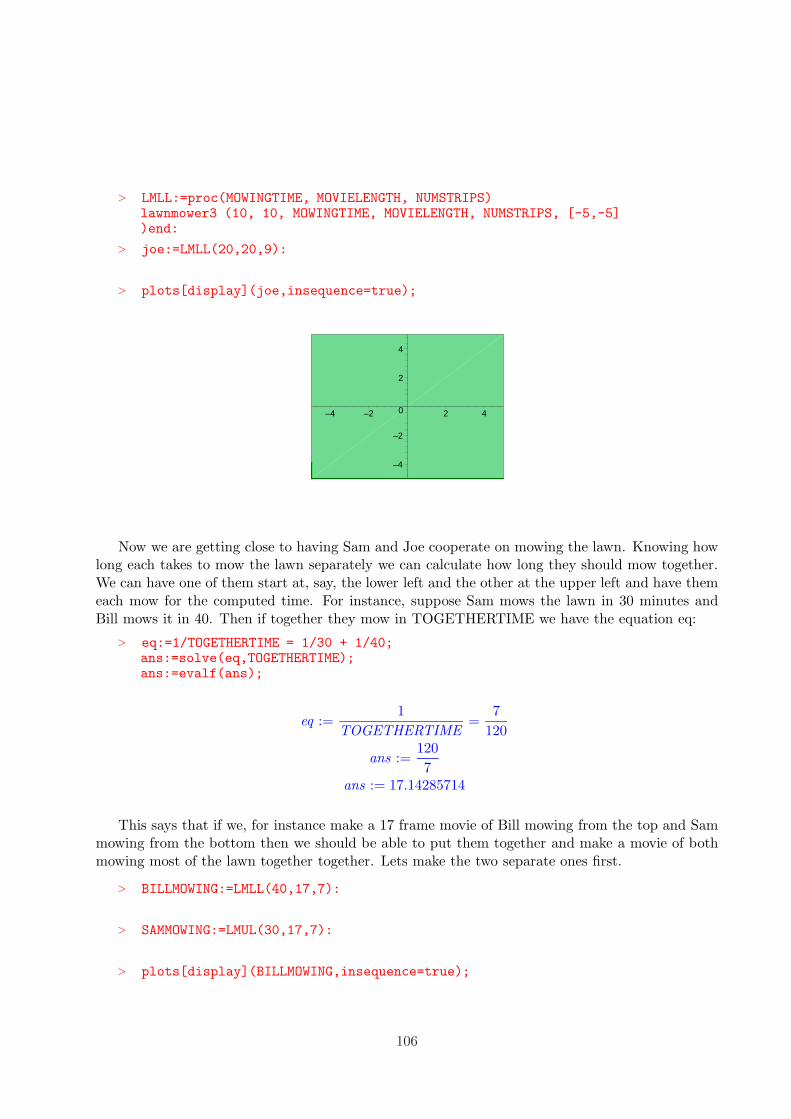
> LMLL:=proc(MOWINGTIME, MOVIELENGTH, NUMSTRIPS)lawnmower3 (10, 10, MOWINGTIME, MOVIELENGTH, NUMSTRIPS, [-5,-5])end:

> joe:=LMLL(20,20,9):


–4

–2

0

2

4

–4 –2 2 4

Now we are getting close to having Sam and Joe cooperate on mowing the lawn. Knowing howlong each takes to mow the lawn separately we can calculate how long they should mow together.We can have one of them start at, say, the lower left and the other at the upper left and have themeach mow for the computed time. For instance, suppose Sam mows the lawn in 30 minutes andBill mows it in 40. Then if together they mow in TOGETHERTIME we have the equation eq:

> eq:=1/TOGETHERTIME = 1/30 + 1/40;ans:=solve(eq,TOGETHERTIME);ans:=evalf(ans);

eq :=1

TOGETHERTIME=

7

120

ans :=120

7ans := 17.14285714

This says that if we, for instance make a 17 frame movie of Bill mowing from the top and Sammowing from the bottom then we should be able to put them together and make a movie of bothmowing most of the lawn together together. Lets make the two separate ones first.

> BILLMOWING:=LMLL(40,17,7):

> SAMMOWING:=LMUL(30,17,7):

> plots[display](BILLMOWING,insequence=true);

106

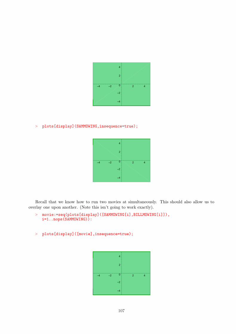
–4

–2

0

2

4

–4 –2 2 4

> plots[display](SAMMOWING,insequence=true);

–4

–2

0

2

4

–4 –2 2 4

Recall that we know how to run two movies at simultaneously. This should also allow us tooverlay one upon another. (Note this isn’t going to work exactly).

> movie:=seq(plots[display]([SAMMOWING[i],BILLMOWING[i]]),i=1..nops(SAMMOWING)):


–4

–2

0

2

4

–4 –2 2 4

107

There are two problems. One is that the movie only has our mowers mowing 17 time unitswhile it takes a little more than that to finish the job. The other is that we have one movie playingon top of the other SAMMOWING is on top of BILLMOWING. This would be ok except thateach frame of SAMMOWING also puts down the unnown lawn as a base. Thus we need a slightlymodified version of SAMMOWING in which the base isn’t put down. We just need to go backand modify lawnmower4y to lawnmower4y without background. The reader should compare thefollowing to lawnmower4y. All we have done is delete the background (YARD) from each frame toget ”lawnmower4 without background”. Note that the deletions are accomplished by ”commenting”out the definition of ”YARD” and references to ”YARD” in ”lawnmower4y”.

> lm4ywobg:=proc(Lngth, Wdth, MOWINGTIME, MOVIELENGTH, NUMSTRIPS, SHIFT)local movie, YARD, MOWEDYARD, MRWDTH, TIME, WHICHSTRIP, FRACSTRIP,

> MOWN, FRAME, LASTFRAME ;movie:=NULL:#YARD:=lawnreflxeq3([0,0],[Lngth , 0],[Lngth ,Wdth ],[ 0,Wdth ],

> aquamarine,SHIFT):MOWEDYARD:=lawny([0,0],[Lngth , 0],[Lngth ,Wdth ],[ 0,Wdth ],green,SHIFT):


> WHICHSTRIP:= floor(NUMSTRIPS*TIME/MOWINGTIME);FRACSTRIP:=TIME*(NUMSTRIPS/MOWINGTIME) - WHICHSTRIP;MOWN:=lawny(


> FRAME:=plots[display]([MOWN, lawny( [0,MRWDTH*(WHICHSTRIP )] ,[Lngth *FRACSTRIP,MRWDTH*(WHICHSTRIP )],[Lngth*FRACSTRIP,MRWDTH*(WHICHSTRIP+1) ],[0,MRWDTH*(WHICHSTRIP+1)],

> green,SHIFT ) ] # ,YARD):else

> FRAME:=plots[display]([MOWN, lawny([Lngth *(1-FRACSTRIP),MRWDTH*(WHICHSTRIP )], [Lngth,MRWDTH*(WHICHSTRIP )],[Lngth,MRWDTH*(WHICHSTRIP+1)], [Lngth *( 1-

> FRACSTRIP),MRWDTH*(WHICHSTRIP+1) ] , green,SHIFT ) ] #,YARD):fi:

> movie:=movie,FRAME:elsemovie:=movie,MOWEDYARD:

> fi:od:if MOVIELENGTH >= MOWINGTIME then LASTFRAME:=MOWEDYARD:

> movie:=movie,LASTFRAME:plots[display]([movie],insequence=true):fi:[movie];end:

Now we can make the associated ”lawn mower upper left without background”

108

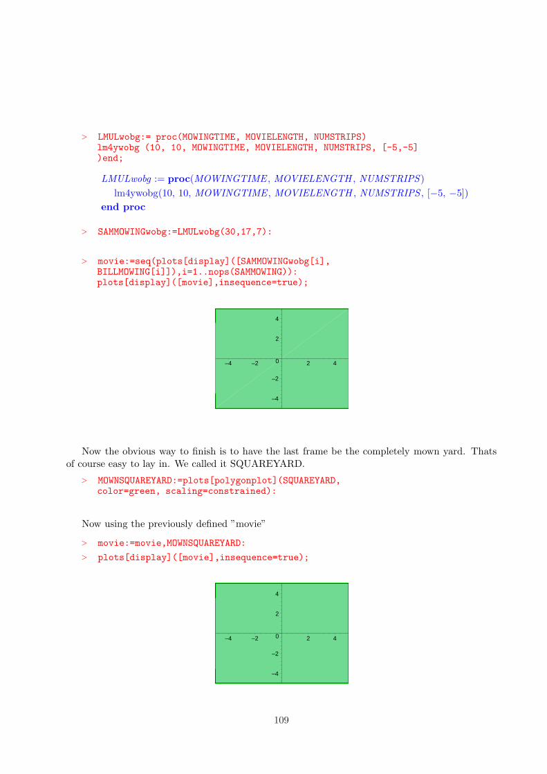
> LMULwobg:= proc(MOWINGTIME, MOVIELENGTH, NUMSTRIPS)lm4ywobg (10, 10, MOWINGTIME, MOVIELENGTH, NUMSTRIPS, [-5,-5])end;

LMULwobg := proc(MOWINGTIME , MOVIELENGTH , NUMSTRIPS)

lm4ywobg(10, 10, MOWINGTIME , MOVIELENGTH , NUMSTRIPS , [−5, −5])

end proc

> SAMMOWINGwobg:=LMULwobg(30,17,7):

> movie:=seq(plots[display]([SAMMOWINGwobg[i],BILLMOWING[i]]),i=1..nops(SAMMOWING)):plots[display]([movie],insequence=true);

–4

–2

0

2

4

–4 –2 2 4

Now the obvious way to finish is to have the last frame be the completely mown yard. Thatsof course easy to lay in. We called it SQUAREYARD.

> MOWNSQUAREYARD:=plots[polygonplot](SQUAREYARD,color=green, scaling=constrained):

Now using the previously defined ”movie”

> movie:=movie,MOWNSQUAREYARD:


–4

–2

0

2

4

–4 –2 2 4

109

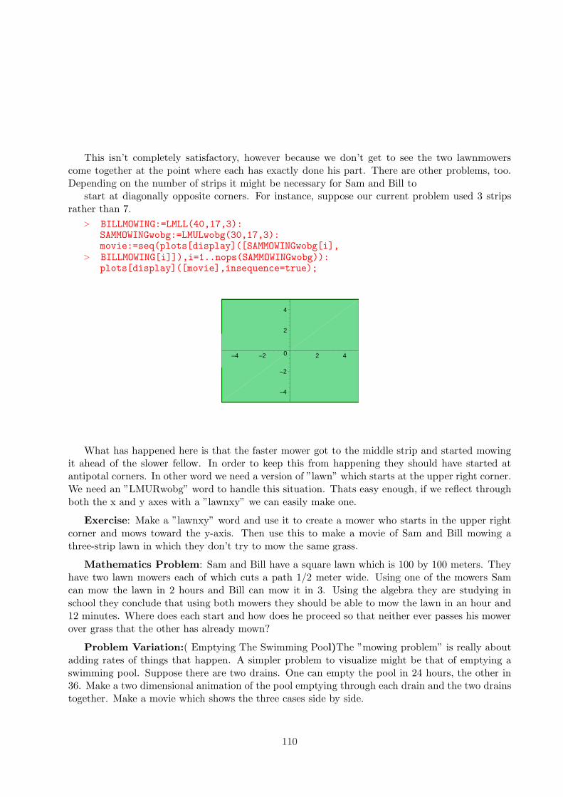
This isn’t completely satisfactory, however because we don’t get to see the two lawnmowerscome together at the point where each has exactly done his part. There are other problems, too.Depending on the number of strips it might be necessary for Sam and Bill to

start at diagonally opposite corners. For instance, suppose our current problem used 3 stripsrather than 7.

> BILLMOWING:=LMLL(40,17,3):SAMMOWINGwobg:=LMULwobg(30,17,3):movie:=seq(plots[display]([SAMMOWINGwobg[i],

> BILLMOWING[i]]),i=1..nops(SAMMOWINGwobg)):plots[display]([movie],insequence=true);

–4

–2

0

2

4

–4 –2 2 4

What has happened here is that the faster mower got to the middle strip and started mowingit ahead of the slower fellow. In order to keep this from happening they should have started atantipotal corners. In other word we need a version of ”lawn” which starts at the upper right corner.We need an ”LMURwobg” word to handle this situation. Thats easy enough, if we reflect throughboth the x and y axes with a ”lawnxy” we can easily make one.

Exercise: Make a ”lawnxy” word and use it to create a mower who starts in the upper rightcorner and mows toward the y-axis. Then use this to make a movie of Sam and Bill mowing athree-strip lawn in which they don’t try to mow the same grass.

Mathematics Problem: Sam and Bill have a square lawn which is 100 by 100 meters. Theyhave two lawn mowers each of which cuts a path 1/2 meter wide. Using one of the mowers Samcan mow the lawn in 2 hours and Bill can mow it in 3. Using the algebra they are studying inschool they conclude that using both mowers they should be able to mow the lawn in an hour and12 minutes. Where does each start and how does he proceed so that neither ever passes his mowerover grass that the other has already mown?

Problem Variation:( Emptying The Swimming Pool)The ”mowing problem” is really aboutadding rates of things that happen. A simpler problem to visualize might be that of emptying aswimming pool. Suppose there are two drains. One can empty the pool in 24 hours, the other in36. Make a two dimensional animation of the pool emptying through each drain and the two drainstogether. Make a movie which shows the three cases side by side.

110

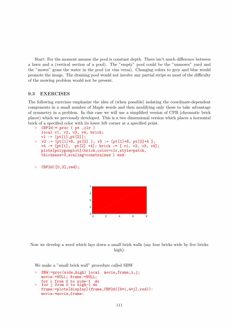
Start: For the moment assume the pool is constant depth. There isn’t much difference betweena lawn and a (vertical section of a pool). The ”empty” pool could be the ”unmown” yard andthe ”mown” grass the water in the pool (or visa versa). Changing colors to grey and blue wouldpromote the image. The draining pool would not involve any partial strips so most of the difficultyof the mowing problem would not be present.

9.3 EXERCISES

The following exercises emphasize the idea of (when possible) isolating the coordinate-dependentcomponents in a small number of Maple words and then modifying only those to take advantageof symmetry in a problem. In this case we will use a simplified version of CPB (chromatic brickplacer) which we previously developed. This is a two dimensional version which places a horzontalbrick of a specified color with its lower left corner at a specified point.

> CBP2d:= proc ( pt ,clr )local v1, v2, v3, v4, brick;v1 := [pt[1],pt[2]];

> v2 := [pt[1]+8, pt[2] ]; v3 := [pt[1]+8, pt[2]+4 ];v4 := [pt[1], pt[2] +4]; brick := [ v1, v2, v3, v4];plots[polygonplot](brick,color=clr,style=patch,thickness=3,scaling=constrained ) end:

> CBP2d([0,3],red);

3

4

5

6

7

0 2 4 6 8

Now we develop a word which lays down a small brick walls (say four bricks wide by five brickshigh):

We make a ”small brick wall” procedure called SBW

> SBW:=proc(wide,high) local movie,frame,i,j;movie:=NULL; frame:=NULL;for i from 0 to wide-1 do

> for j from 0 to high-1 doframe:=plots[display](frame,CBP2d([8*i,4*j],red)):movie:=movie,frame:

111

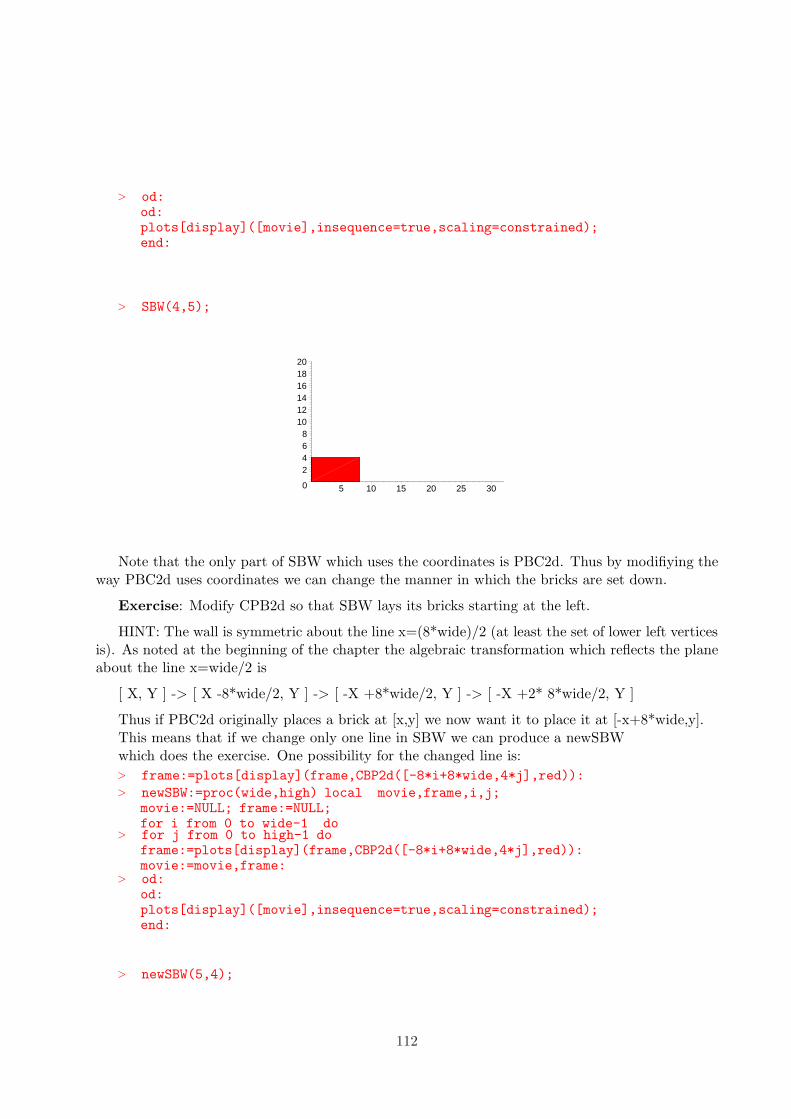
> od:od:plots[display]([movie],insequence=true,scaling=constrained);end:

> SBW(4,5);

0

2468

101214161820

5 10 15 20 25 30

Note that the only part of SBW which uses the coordinates is PBC2d. Thus by modifiying theway PBC2d uses coordinates we can change the manner in which the bricks are set down.

Exercise: Modify CPB2d so that SBW lays its bricks starting at the left.

HINT: The wall is symmetric about the line x=(8*wide)/2 (at least the set of lower left verticesis). As noted at the beginning of the chapter the algebraic transformation which reflects the planeabout the line x=wide/2 is

[ X, Y ] -> [ X -8*wide/2, Y ] -> [ -X +8*wide/2, Y ] -> [ -X +2* 8*wide/2, Y ]

Thus if PBC2d originally places a brick at [x,y] we now want it to place it at [-x+8*wide,y].This means that if we change only one line in SBW we can produce a newSBWwhich does the exercise. One possibility for the changed line is:> frame:=plots[display](frame,CBP2d([-8*i+8*wide,4*j],red)):> newSBW:=proc(wide,high) local movie,frame,i,j;

movie:=NULL; frame:=NULL;for i from 0 to wide-1 do

> for j from 0 to high-1 doframe:=plots[display](frame,CBP2d([-8*i+8*wide,4*j],red)):movie:=movie,frame:

> od:od:plots[display]([movie],insequence=true,scaling=constrained);end:

> newSBW(5,4);

112

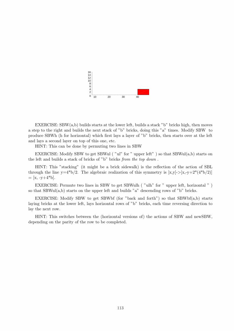
0

2468

10121416

10 20 30 40

EXERCISE: SBW(a,b) builds starts at the lower left, builds a stack ”b” bricks high, then movesa step to the right and builds the next stack of ”b” bricks, doing this ”a” times. Modify SBW toproduce SBWh (h for horizontal) which first lays a layer of ”b” bricks, then starts over at the leftand lays a second layer on top of this one, etc.

HINT: This can be done by permuting two lines in SBW

EXERCISE: Modify SBW to get SBWul ( ”ul” for ” upper left” ) so that SBWul(a,b) starts onthe left and builds a stack of bricks of ”b” bricks from the top down .

HINT: This ”stacking” (it might be a brick sidewalk) is the reflection of the action of SBLthrough the line y=4*b/2. The algebraic realization of this symmetry is [x,y]->[x,-y+2*(4*b/2)]= [x, -y+4*b].

EXERCISE: Permute two lines in SBW to get SBWulh ( ”ulh” for ” upper left, horizontal ” )so that SBWul(a,b) starts on the upper left and builds ”a” descending rows of ”b” bricks.

EXERCISE: Modify SBW to get SBWbf (for ”back and forth”) so that SBWbf(a,b) startslaying bricks at the lower left, lays horizontal rows of ”b” bricks, each time reversing direction tolay the next row.

HINT: This switches between the (horizontal versions of) the actions of SBW and newSBW,depending on the parity of the row to be completed.

113

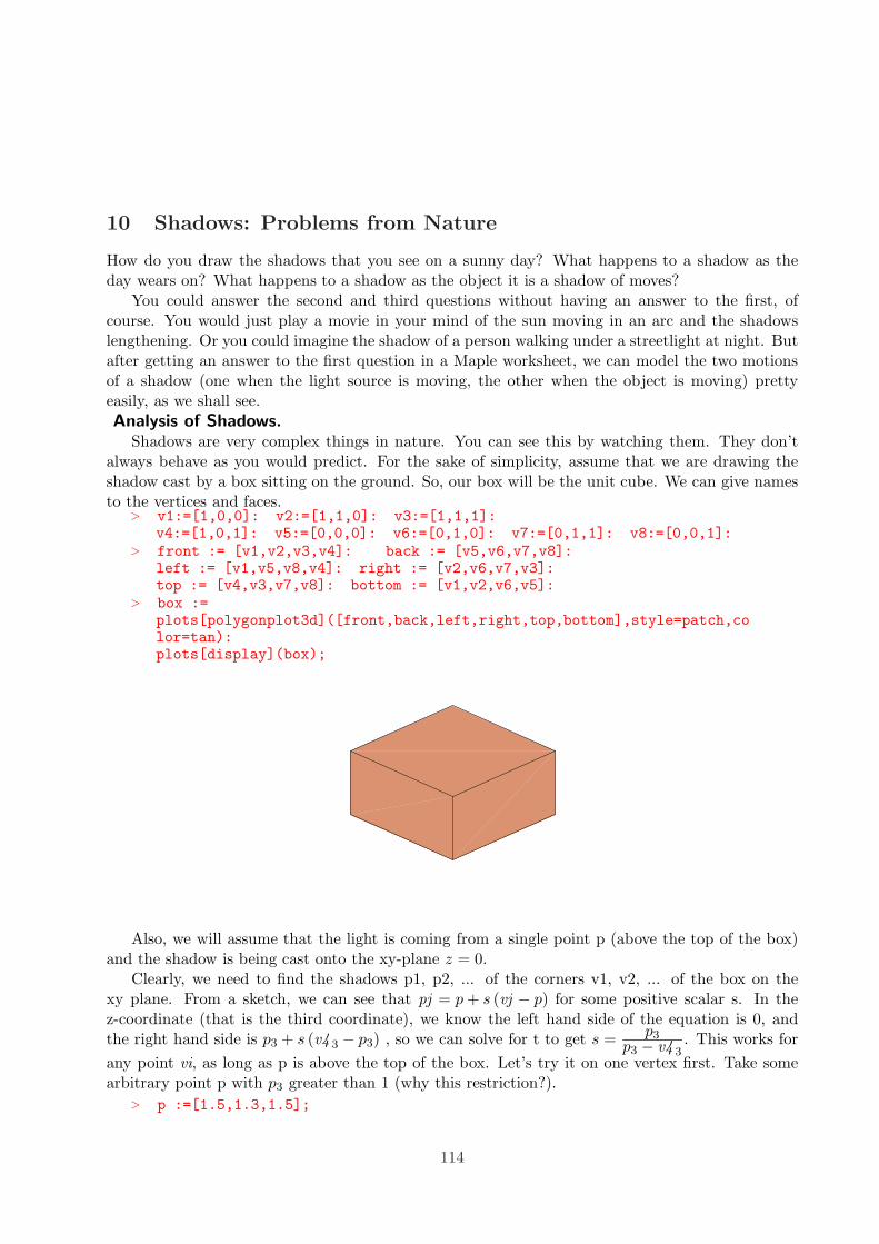
10 Shadows: Problems from Nature

How do you draw the shadows that you see on a sunny day? What happens to a shadow as theday wears on? What happens to a shadow as the object it is a shadow of moves?

You could answer the second and third questions without having an answer to the first, ofcourse. You would just play a movie in your mind of the sun moving in an arc and the shadowslengthening. Or you could imagine the shadow of a person walking under a streetlight at night. Butafter getting an answer to the first question in a Maple worksheet, we can model the two motionsof a shadow (one when the light source is moving, the other when the object is moving) prettyeasily, as we shall see.

Analysis of Shadows.Shadows are very complex things in nature. You can see this by watching them. They don’t

always behave as you would predict. For the sake of simplicity, assume that we are drawing theshadow cast by a box sitting on the ground. So, our box will be the unit cube. We can give namesto the vertices and faces.

> v1:=[1,0,0]: v2:=[1,1,0]: v3:=[1,1,1]:v4:=[1,0,1]: v5:=[0,0,0]: v6:=[0,1,0]: v7:=[0,1,1]: v8:=[0,0,1]:

> front := [v1,v2,v3,v4]: back := [v5,v6,v7,v8]:left := [v1,v5,v8,v4]: right := [v2,v6,v7,v3]:top := [v4,v3,v7,v8]: bottom := [v1,v2,v6,v5]:

> box :=plots[polygonplot3d]([front,back,left,right,top,bottom],style=patch,color=tan):plots[display](box);

Also, we will assume that the light is coming from a single point p (above the top of the box)and the shadow is being cast onto the xy-plane z = 0.

Clearly, we need to find the shadows p1, p2, ... of the corners v1, v2, ... of the box on thexy plane. From a sketch, we can see that pj = p + s (vj − p) for some positive scalar s. In thez-coordinate (that is the third coordinate), we know the left hand side of the equation is 0, andthe right hand side is p3 + s (v4 3 − p3) , so we can solve for t to get s =

p3p3 − v4 3

. This works for

any point vi, as long as p is above the top of the box. Let’s try it on one vertex first. Take somearbitrary point p with p3 greater than 1 (why this restriction?).

> p :=[1.5,1.3,1.5];

114

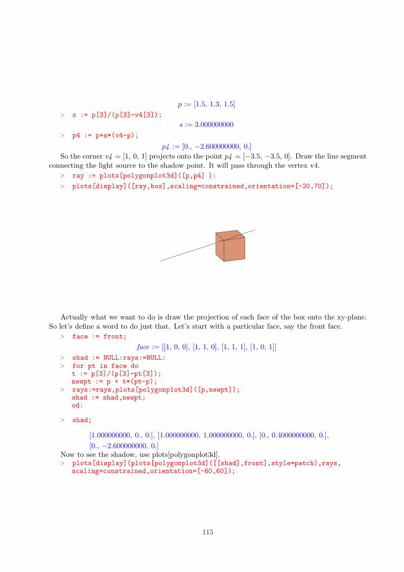
p := [1.5, 1.3, 1.5]

> s := p[3]/(p[3]-v4[3]);

s := 3.000000000

> p4 := p+s*(v4-p);

p4 := [0., −2.600000000, 0.]

So the corner v4 = [1, 0, 1] projects onto the point p4 = [−3.5, −3.5, 0]. Draw the line segmentconnecting the light source to the shadow point. It will pass through the vertex v4.

> ray := plots[polygonplot3d]([p,p4] ):

> plots[display]([ray,box],scaling=constrained,orientation=[-20,70]);

Actually what we want to do is draw the projection of each face of the box onto the xy-plane.So let’s define a word to do just that. Let’s start with a particular face, say the front face.

> face := front;

face := [[1, 0, 0], [1, 1, 0], [1, 1, 1], [1, 0, 1]]

> shad := NULL:rays:=NULL:> for pt in face do

t := p[3]/(p[3]-pt[3]);newpt := p + t*(pt-p);

> rays:=rays,plots[polygonplot3d]([p,newpt]);shad := shad,newpt;od:

> shad;

[1.000000000, 0., 0.], [1.000000000, 1.000000000, 0.], [0., 0.4000000000, 0.],

[0., −2.600000000, 0.]Now to see the shadow, use plots[polygonplot3d].> plots[display](plots[polygonplot3d]([[shad],front],style=patch),rays,

scaling=constrained,orientation=[-60,60]);

115

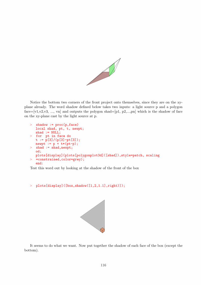
Notice the bottom two corners of the front project onto themselves, since they are on the xy-plane already. The word shadow defined below takes two inputs: a light source p and a polygonface=[v1,v2,v3, ..., vn] and outputs the polygon shad=[p1, p2,...,pn] which is the shadow of faceon the xy-plane cast by the light source at p.

> shadow := proc(p,face)local shad, pt, t, newpt;shad := NULL;

> for pt in face dot := p[3]/(p[3]-pt[3]);newpt := p + t*(pt-p);

> shad := shad,newpt;od;plots[display](plots[polygonplot3d]([shad]),style=patch, scaling

> =constrained,color=grey);end:

Test this word out by looking at the shadow of the front of the box

> plots[display]([box,shadow([1,2,1.1],right)]);

It seems to do what we want. Now put together the shadow of each face of the box (except thebottom).

116

> shadowbox := p ->plots[display]([plots[pointplot3d](p,thickness=100,color=red,symbol=cross),box,shadow(p,front),shadow(p,top),shadow(p,left),shadow(p,right), shadow(p,back)] ):

> shadowbox([1.2,1.6,1.5]);

10.1 Problems:

1. Find the area of the shadow shown above, not counting the base of the box. Hint: Redraw withaxes = boxed and notice the shadow ’sits’ in a rectangle.

2. Modify the definition for shadowbox so that box could be any collection of faces, not justthe faces of the box. Use the newly defined word to draw the shadow of a box that is raised off ofthe xy-plane.

3. Shadows cast by the light of the sun or some far off light source are traced out by parallellight rays, rather than rays coming from a point p. Develop a word pshadow which draws such ashadow and use it to draw a shadowbox.

Solution to 3.> pshadow := proc(dir,face)

local shad, pt, t, newpt;shad := NULL;

> for pt in face dot := pt[3]/(-dir[3]);newpt := pt + t*dir;

> shad := shad,newpt;od;plots[polygonplot3d]([shad],style=patch, scaling

> =constrained,color=grey);end:

> pshadowbox := p -> plots[display]([box,pshadow(p,front),pshadow(p,top),pshadow(p,left),pshadow(p,right),pshadow(p,back)] ):

> dir := [1,1,2]:

> pshadowbox([.5,2,1]);

117

10.2 Moving shadows

Now to make the shadows move, all we need to do is move the light source, taking pictures as itmoves. While we’re at it, we can provide a tabletop for the shadow to move on.

> tabletop := plots[polygonplot3d]([[-2,-4,-.01],[2,-4,-.01],[2,2,-.01],[-2,2,-.01]],color=magenta,style=patch):

> movie := [seq(plots[display]([tabletop,shadowbox(q+[ i,i/2,0])]),i=0..20)]:


Moving Shadow Problem Make a movie of the shadow of the box as it moves from its positionat the origin to the point [0,0,3] above the xy-plane. Keep the light source fixed at q=[-5,23,8]. Useyour definition of shadowbox from the last problem.

11 More Exercises

Exercise: Modify the vertices of ”box” below to make a ”lightpole”with the unit square as base and 3 units high. This can be done by modifying the following

instructions.

118

> v1:=[.5,0,0]: v2:=[.5,.5,0]: v3:=[.5,.5,3]: v4:=[.5,0,3]:v5:=[0,0,0]: v6:=[0,.5,0]: v7:=[0,.5,3]: v8:=[0,0,3]:front := [v1,v2,v3,v4]: back := [v5,v6,v7,v8]:

> left := [v1,v5,v8,v4]: right := [v2,v6,v7,v3]:top := [v4,v3,v7,v8]: bottom := [v1,v2,v6,v5]:pole :=

> plots[polygonplot3d]([front,back,left,right,top,bottom],style=patch,color=tan,scaling=constrained):

EXERCISE: Use plottool[sphere] to place a light on top of the pole in the form of a sphere oneunit in diameter.

EXERCISE: Place the lightpole on a rectangular area according to the diagram.

–4

–2

0

2

4

–4 –2 2 4 6 8 10

11.1 DIAGRAM CODE

> base:=plots[polygonplot]([ [-.5,-.5], [ .5,-.5], [ .5,.5],[-.5,.5]], style=patch,color=tan, scaling=constrained):ground:=plots[polygonplot]([[ -5,-5 ],[ 10,-5 ],[ 10, 5 ],[ -5, 5

> ]],color=green, style=patch ):plots[display]([base, ground],scaling=constrained);

11.2 GROUND PLACEMENT

> light:=plottools[sphere]( [.5,.5,4], 1,color=red,style=patchnogrid):ground:=plots[polygonplot3d]([[ -5,-5,0],[ 10,-5,0],[ 10, 5,0],[ -5,

> 5,0]],color=green, style=patch ):

Exercise: Errect a wall 10 units from the light pole which is ten units high, as indicated in thediagram

119

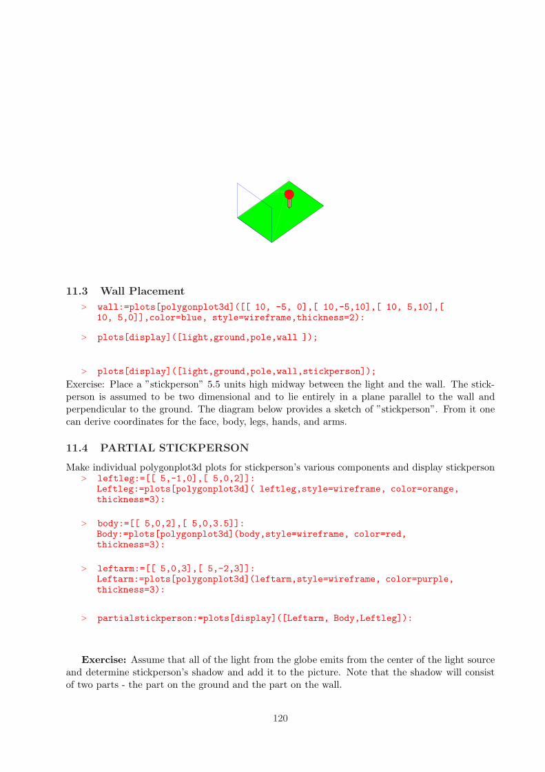
11.3 Wall Placement

> wall:=plots[polygonplot3d]([[ 10, -5, 0],[ 10,-5,10],[ 10, 5,10],[10, 5,0]],color=blue, style=wireframe,thickness=2):

> plots[display]([light,ground,pole,wall ]);

> plots[display]([light,ground,pole,wall,stickperson]);

Exercise: Place a ”stickperson” 5.5 units high midway between the light and the wall. The stick-person is assumed to be two dimensional and to lie entirely in a plane parallel to the wall andperpendicular to the ground. The diagram below provides a sketch of ”stickperson”. From it onecan derive coordinates for the face, body, legs, hands, and arms.

11.4 PARTIAL STICKPERSON

Make individual polygonplot3d plots for stickperson’s various components and display stickperson> leftleg:=[[ 5,-1,0],[ 5,0,2]]:

Leftleg:=plots[polygonplot3d]( leftleg,style=wireframe, color=orange,thickness=3):

> body:=[[ 5,0,2],[ 5,0,3.5]]:Body:=plots[polygonplot3d](body,style=wireframe, color=red,thickness=3):

> leftarm:=[[ 5,0,3],[ 5,-2,3]]:Leftarm:=plots[polygonplot3d](leftarm,style=wireframe, color=purple,thickness=3):

> partialstickperson:=plots[display]([Leftarm, Body,Leftleg]):

Exercise: Assume that all of the light from the globe emits from the center of the light sourceand determine stickperson’s shadow and add it to the picture. Note that the shadow will consistof two parts - the part on the ground and the part on the wall.

120

Exercise: Make an animation in which the light moves toward stickman. Make the shadowmove appropriately.

Exercise: Put a flag in stickman’s hand and extend the shadow to include the flag.Exercise: Animate stickman to the extent that he/she waves the flag, extend the animation

to include the flag shadow.Exercise: Make stickperson’s head a (three dimensional) cube and extend the shadow.

121

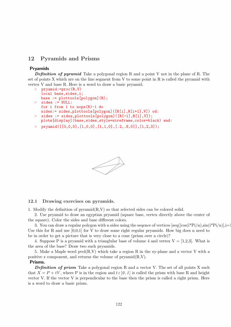
12 Pyramids and Prisms

PryamidsDefinition of pyramid Take a polygonal region R and a point V not in the plane of R. The

set of points X which are on the line segment from V to some point in R is called the pyramid withvertex V and base R. Here is a word to draw a basic pryamid.

> pryamid:=proc(R,V)local base,sides,i;base := plottools[polygon](R);

> sides := NULL:for i from 1 to nops(R)-1 dosides:= sides,plottools[polygon]([R[i],R[i+1],V]) od:

> sides := sides,plottools[polygon]([R[-1],R[1],V]);plots[display](base,sides,style=wireframe,color=black) end:

> pryamid([[0,0,0],[1,0,0],[1,1,0],[.2,.8,0]],[1,2,3]);

12.1 Drawing exercises on pyramids.

1. Modify the definition of pyramid(R,V) so that selected sides can be colored solid.2. Use pryamid to draw an egyptian pryamid (square base, vertex directly above the center of

the square). Color the sides and base different colors.3. You can draw a regular polygon with n sides using the seqence of vertices [seq([cos(i*Pi/n),sin(i*Pi/n)],i=1..n)].

Use this for R and use [0,0,1] for V to draw some right regular pryamids. How big does n need tobe in order to get a picture that is very close to a cone (prism over a circle)?

4. Suppose P is a pryamid with a trianglular base of volume 4 and vertex V = [1,2,3]. What isthe area of the base? Draw two such pryamids.

5. Make a Maple word pvol(R,V) which take a region R in the xy-plane and a vector V with apositive z component, and returns the volume of pryamid(R,V).

Prisms.Definition of prism Take a polygonal region R and a vector V. The set of all points X such

that X = P + tV , where P is in the region and t ε [0 , 1 ] is called the prism with base R and heightvector V. If the vector V is perpendicular to the base then the prism is called a right prism. Hereis a word to draw a basic prism.

122

> prism:=proc(R,V)local base,sides,i;base := plottools[polygon](R);

> sides := NULL:for i from 1 to nops(R)-1 dosides:= sides,plottools[polygon]([R[i],R[i+1],R[i+1]+V,R[i]+V]) od:

> sides := sides,plottools[polygon]([R[-1],R[1],R[1]+V,R[-1]+V]);plots[display](base,sides,style=wireframe,color=black) end:

> prism([[0,0,0],[1,0,0],[1,1,0],[.2,.8,0]],[1,2,3]);

The top of the prism with base R and height vector V is defined to be the set of all points Xsuch that X = P + V , where P is in R. Note that the top of the prism is the translate of the baseby adding V. So it is congruent to the base.

12.2 Exercises on prisms

1. Modify the definition of the word prism(R,V) to include a color option.2. Is a cube a prism? What about a tetrahedron?3. What is another name for this prism? prism([[0,0,0],[2,0,0],[2,0,1],[1,0,2],[0,0,1]],[0,2,0])4. Suppose P is a prism with a trianglular base of volume 4 and height 2. What is the area of

the base? Draw two such prisms.5. Make a Maple word pvol(R,V) which take a region R in the xy-plane and a vector V with a

positive z componen, and returns the volume of prism(R,V).

12.3 Cross Sections of pyramids and prisms

Take a pyramid and a plane which cuts the vertex away from the base. The intersection of theplane with the pyramid is called a cross section of the pyramid. Similarly, a cross section of a prismis the intersection of the prism with a plane which cuts the top from the base of the prism. In eachcase, the plane which is used to form the cross section is called the cross sectioning plane.

Theorem about cross sections of a prism. Parallel cross sections of a prism arecongruent. (Note: two cross sections are parallel if their cross sectioning planes are parallel.)

Proof: Take any side AB(B+v)(A+V) of the prism. The two parallel planes intersect thisside in two parallel segments A’B’ and A”B”, where A’ and A” are on the segment A(A+V),labelled with A’ between A and A” and B’ and B” are on B(B+V), labelled with B’ between B

123

and B”. The segments A’A” and B’B” are parallel, since they are both parallel to the vector V.So the quadrilateral A’B’B”A” is a parallelogram. Let U be the vector from A’ to A”. Then sinceA’B’B”A” is a parallogram, B” = B’ + U. Continue all the way around the cross section containingA’, and use the same argument to show that the vertices on the cross section containing A” areall of the from X” = X’+U, where X’ is a vertex on the cross section containing A’ . This meansthat the cross section containing A” is the translate of cross section containing A’ by adding U. Sothese cross sections are congruent by translation. qed

Theorem about cross sections of a pyramid. Parallel cross sections of a pyramidare similar.

Proof. We can assume (by translating if need be) that the vertex of the pyramid is at theorigin. Take any one of the sides ABV of the pyramid. The two parallel planes intersect this sidein two parallel segments A’B’ and A1B1, where A’ and A1=A” are on the segment AV, labelledwith A’ between A and A1 and B’ and B1=B” are on BV, labelled with B’ between B and B”. Sothe angles VA’B’ and VA”B” are congruent, since they are corresponding angles of the transversalVA of the parallel lines A’B’ and A”B”. Then the triangles VA’B’ and VA1B1 are similar sincecorresponding angles are congruent. Hence corresponding sides are proportional. In particular,VA′

VA1 = VB ′

VB1. Call this constant of proportionality k. Then for each vertex X of the cross section containing

A’, the point X1 = kX ′ is a vertex of the cross section containing A1. Hence the cross sectioncontaining A’ is carried onto the cross section containing A1 by the similiarity transformationX → kX . qed

Exercises on cross sections of a prism.

Exercise: Show that the converse of the theorem about prisms is false, by finding two congruentcross sections of a cube which are not parallel.

Exercise: Define a maple word crossect(base,vertex,plane) which takes a polygonal base, aheight vector, and an equation for a cross sectioning plane and returns the polygonal cross sectionof the prism.

124

13 Cross Sections of triangular prisms

13.1 The Theorem and its proof.

Theorem: If P is a triangular prism of sufficient height and T is any triangle then there is a planewhose intersection with P is similar to T.

We will prove the following restatement of the theorem:Let ABC and PQR be any triangles in the x-y plane, K the vector [0,0,1] and s,t any numbers.

Then s and t may be chosen so that the triangle C(A+tK)(B+sK) is similar to PQR..

Proof: Then the theorem asserts that given any other triangle PQR we can choose t and s sothat the triangle (A+tK)C(B+sK) is similar to PQR. The two triangles are similar if two legs areproportional and the included angles are equal (”side angle side”).

Place the triangle ABC (or one similar to it) so that C=[0,0,0], B=[1,0,0], and A=[a,b,0] witha,b positive. Place the triangle PQR (or one similar to it) so that P=A, Q=C, and R=[p,q,r] withp,r positive. Then we want to choose s and t so that the angle((A + t K)C (B + s K)) has the samecosine as QPR and the lengths of the vectors A+tK and B+tK are proportional to QP and RP,the legs of QPR by some factor k. We have arranged for C and P to be the origin so that we canuse that the cosine of the angle between two vectors is their dot product divided by the productsof their lengths. We then have the three equations:

dotprod(A + tK , B + tK )length(A + t K) length(B + s K)

=dotprod(Q, R)

length(Q) length(R)

and the other two are

length(A+tK) = k length(Q)

length(B+sK) = k length(R)

Using the second two equations in the denominators of the first and knowing that the dotproduct of Q and R is p we have, on substitution the three equations:

dotprod(A + tK , B + sK ) = k2 p,

length(A + t K) = k,

length(B + s K) = k2 (p2 + q2)

125

Putting these into Maplese (it turns out to be convenient to assume p,q, s, and t are real.)

> p:=’p’:q:=’q’:s:=’s’: t:=’t’:a:=’a’: b:=’b’:assume(p,real,q,real,s,real,t,real,a,real,b,real):interface(showassumed=0);

1> A:=[a,b,0]: B:=[1,0,0]: C:=[0,0,0]:K:=[0,0,1]:

P:=[0,0,0]:Q:=[1,0,0]:R:=[p,q,0]:eq1 := linalg[dotprod](A + t*K,B + s*K) = k^2*p;

> eq2 := linalg[dotprod](A + t*K,A + t*K) = k^2;eq3 := linalg[dotprod](B + s*K,B + s*K) = k^2*(p^2 + q^2);

eq1 := a + t s = k2 p

eq2 := a2 + b2 + t2 = k2

eq3 := 1 + s2 = k2 (p2 + q2)

Use eq2 to eliminate kˆ2 from the first and third euqations.

> EQ1:= lhs(eq1)=lhs(eq2)*p;EQ2:=lhs(eq3)=lhs(eq2)*(p^2+q^2);

EQ1 := a + t s = (a2 + b2 + t2) p

EQ2 := 1 + s2 = (a2 + b2 + t2) (p2 + q2)

We can solve for values of s and t which satisfy these equations by:

> sol:=solve({EQ1,EQ2},{s,t});

sol := {s =−a + p a2 + p b2 + p %12

%1, t = %1}

%1 := RootOf( Z 4 q2 + (−1 − a2 p2 + 2 a p − b2 p2 + a2 q2 + b2 q2) Z 2 − p2 b4 − a2

+ 2 p a3 + 2 a p b2 − p2 a4 − 2 p2 a2 b2)

This tells us that if at least one of the values of t is non-zero and real then there is a solution.

> tsol:=(sol[2]);

tsol := t = RootOf( Z 4 q2 + (−1 − a2 p2 + 2 a p − b2 p2 + a2 q2 + b2 q2) Z 2 − p2 b4 − a2

+ 2 p a3 + 2 a p b2 − p2 a4 − 2 p2 a2 b2)

By inspection we see that although tsol is a root of a polynomial which is quadratic in Z 2. Wemight work with the quadratic by substituting

√X for Z and stripping out the resulting quadratic

in X.

> p2:=op(rhs(subs(_Z=sqrt(X),tsol)));

p2 := X2 q2 + (−1 − a2 p2 + 2 a p − b2 p2 + a2 q2 + b2 q2)X − p2 b4 − a2 + 2 p a3 + 2 a p b2

− p2 a4 − 2 p2 a2 b2

Thus in order for for there to be a non-zero and positive value for t we must find a positive root

126

to p2.Since the lead coefficient of p2 is the positive number 256 q2 its graph is a upward-opening

parabola which crosses the x-axis twice if p2(z) is negative for some value of z. (The ”twice” isimportant since we need a non-zero root): if there are two roots one of them must be non-zero. Infact ”const”, the constant term of p2 is the negative of a square.

> const:=subs(X=0,p2);const:=factor(const);

const := −p2 b4 − a2 + 2 p a3 + 2 a p b2 − p2 a4 − 2 p2 a2 b2

const := −(−a + p a2 + p b2)2

If conts is nonzero, the polynomial will have two real roots. We can easily find when the constantis zero by solving

> solve(const,p);

a

a2 + b2 ,a

a2 + b2

Thus const is zero if and only if p = aa2 + b2 . and we must deal with this possibility. If it

happens then we can incorporate this into the original equations and solve again.

> EQ1a:=subs(p=a/(a^2+b^2),EQ1);EQ2a:=subs(p=a/(a^2+b^2),EQ2);SLNS:=solve({EQ1a,EQ2a},{s,t});

EQ1a := a + t s =(a2 + b2 + t2) a

a2 + b2

EQ2a := 1 + s2 = (a2 + b2 + t2) (a2

(a2 + b2)2+ q2)

SLNS := {s = RootOf((a2 + b2) Z 2 − q2 a4 + b2 − 2 q2 a2 b2 − q2 b4), t = 0}, {

s =RootOf((a2 + b2) Z 2 + q2 a4 + 2 q2 a2 b2 + q2 b4 − b2, label = L3 ) a

(a2 + b2) q,

t =RootOf((a2 + b2) Z 2 + q2 a4 + 2 q2 a2 b2 + q2 b4 − b2, label = L3 )

q}

The problem is to see that one of these posibilities is a pair of real numbers. We will have asolution with t=0 if there is a real root to the quadratic

> q1:= (a^2+b^2)*_Z^2-q^2*a^4-2*q^2*b^2*a^2-q^2*b^4+b^2;

q1 := (a2 + b2) Z 2 − q2 a4 + b2 − 2 q2 a2 b2 − q2 b4

Or there will be a solution if the other quadratic has real roots.

> q2:=(a^2+b^2)*_Z^2+q^2*a^4+2*q^2*b^2*a^2+q^2*b^4-b^2;

q2 := (a2 + b2) Z 2 + q2 a4 + 2 q2 a2 b2 + q2 b4 − b2

127

A quadratic has real roots if and only if its discriminant is not-negative so we must see that thediscriminnant of one of q1, q2 is non-negative. In this

> discrim(q1,_Z);discrim(q2,_Z);

4 (a2 + b2) (q2 a4 + 2 q2 a2 b2 + q2 b4 − b2)

−4 (a2 + b2) (q2 a4 + 2 q2 a2 b2 + q2 b4 − b2)

Since each of these discriminants is the negative of the other, one of these quadratics is guar-anteed to have real roots. Hence the problem can be solved, and this proves the theorem. QED.

One value of having an argument like this worked out in Maple is that we can use the argumentto solve specific problems. For instance:

13.2 A prism with an equilateral base and a 3-4-5 right cross-section

Exercise: Cut a triangular prism with an equilateral base so that the cross-section of the cut is a3-4-5 right triangle?

Refering to the original diagram we want ABC to be the equilateral triangle with C=[0,0,0],

B=[1,0,0], and A= [ 12 ,

√3

2 ,0]. We want PQR to be a 3-4-5 triangle. One choice is P=[0,0,0],

Q=[1,0,0], R=[0, 34,0]. Once these are determined the general calculations become specific and we

simply specify:a:=1/2;b:=sqrt(3)/2; p:=0;q:=3/4;

Now we simply follow the calculations in the proof

A:=[a,b,0]; B:=[1,0,0]; C:=[0,0,0];K:=[0,0,1]; P:=[0,0,0];Q:=[1,0,0];R:=[p,q,0]; eq1:=linalg[dotprod](A+t*K,B+s*K)= kˆ2*p; eq2:=linalg[dotprod](A+t*K,A+t*K) = kˆ2; eq3:=linalg[dotprod](B+s*K,B+s*K) =kˆ2*(pˆ2+qˆ2);

Use eq2 to eliminate kˆ2 from the first and third equations

EQ1:= lhs(eq1)=lhs(eq2)*p; EQ2:=lhs(eq3)=lhs(eq2)*(pˆ2+qˆ2);

we can find solve for values of s and t which satisfy these equations by:

ans:=solve({EQ1,EQ2},{s,t});

At this point we are happy with floating point values for s and t.ans:=solve({EQ1,EQ2},{s,t}); ans:=evalf(ans):

128

To get the actual triangles we substitute for s and t in the vertices A+tK, B+tK, and the origin.

ANS:=subs(ans ,[A+s*K,C,B+t*K]); ANS:=expand(ANS);

To check that these are actually the vertices of a 3-4-5 triangle we can calculate the lengths ofthe sides of the triangle. We need a distance function

dist:=proc(X,Y) sqrt((X[1] - Y[1])ˆ2 + (X[2] - Y[2])ˆ2 + (X[3] - Y[3])ˆ2) end;

legs:=[dist(ANS[1],ANS[2]),dist(ANS[2],ANS[3]), dist(ANS[3],ANS[1])];

If this is proportional to a 3-4-5 triangle then the first leg must correspond to one of length 3thus we scale it.

check:=3/legs[1] *legs; check:=expand(check);

13.3 EXERCISES

Exercise: Make a three dimensional Maple plot of the of the figure sketched below. Its base is anequilateral triangle the sides are perpendicular to the base, and the top is a 3-4-5 triangle.

Exercise: Do the previous exercise with the top an isosceles right triangle.Exercise: Suppose f(x) = ax4 + b x3 + c x2 + dx + e with a positive. Suppose there is a z such

that f(z) < 0. Prove that f has at least two different roots.Exercise: Suppose f(x) = ax2 + b x + c with a positive. If c < 0 prove that g(x) = ax4 + b x2 + c

has a real root.

129

14 Exploring Desargues Theorem.

14.1 Points and Lines at Infinity

The principal ”synthetic” tool for determining when one plane figure in space is the shadow ofanother is Desargue’s Theorem which is most properly stated as a theorem in Projective Geometryrather than the cartesian or affine geometry in which we are working. This would be a good placeto begin an enjoyable study of projective geometry, however one of the prinicpal ideas in problemsolving is to learn how to collect, understand, and employ mathematical tools to solve the problemat hand, usually postponing their full development. This often entails extracting a tool, theorem,or technique from its ”natural” milieu and phrasing it and its proof or explanation in the languageof the problem at hand. This often results in much faster progress on the study of the currentproblem purchased at the cost of more lengthy and less elegant statements and arguments. Withregard to the Desargues Theorem we need the notion of ”point at infinity” of a line.

Definition: If L is a line in any number of dimensions) and L is written in parametric formP + t D then we call ”D” the direction of the parameterization. A line has many parameterizationsand different parameterizations may have different directions. , e.g. the parameterization P + t 2.has the 2D as direction. However the directions of any two parameterizations of the same line areproportional (i.e. one is a numerical multiple of the other).

We define the direction of a line L as the totality of all of the directions of its parameterizations.For any line this is an infinite number of things but any two of them are proportional so if we knowone of them we know them all. We use any of its members as a name for the direction of the line.Thus for exampe we say that ” [1,0,0] is the direction of the x-axis”. We also say ”[27,0,0] is thedirection of the x-axis”. What we we would say to be perfectly precise is ”[1.0,0 is a name for thedirection of the x-axis”. However that is too wordy and experience shows that there is no confusionin the ”shorthand” version provided everyone understands the convention. Lest one feel that thisis something new we note that this is exactly the same idea as saying ” 3

2 is the average of 1 and 2”

while ” 64 is the average of 1 and two” is mathematically just as correct. The symbols 1

2 and 64 are

but two of the infinitely many names (numerals) for a particular number. With this introductionwe can now give the following:

Definition: If L is a line then ”the point at infinity on L” is the direction of L.

Example: The point at infinity on the x-axis is the direction [1,0,0]. Note that the ”finite”point [1,0,0] is also on the x-axis but this is different from the direction [1,0,0] which happens to berepersented by the same name. Note that the point at infinity on the x-axis is also the direction[-193,0,0].

Example:What is the point at infinity on the line K which contains the points [1,2,3] and [8,-3,7].

Solution: A parametric equation for ths line is [1,2,3] + t([8,-3,7] - [1,2,3]). Thus the directionof this parameterization of the line is [7,-5,4] so this is one of the names for the direction of the

line, i.e. one of the names for the point at infinity on the line K. [ 1, −57 , 4

7] is another name forthis direction. Note that the ”finite point” [7,-5,4] does not lie on the line K, In the exercises wefind that the ”finite point” with coordinates given by one of the names for the point at infinity ona line will also be on the line if and only if the line goes through the origin.

130

Example: Determine if the line L which contains [1,2,3] and [5,1,2]and the line M which contains [6,0,1] and [3,2,7]] have a point in common (including points at

infinity)

Solution: We can use the Maple solve function to find such points from the parametric forms.L:=expand([1,2,3]+t*([5,1,2]-[1,2,3])); M:=expand([6,0,1]+s*([3,2,7]-[6,0,1])); eq1:= L[1]-M[1]=0;

eq2:=L[2]-M[2]=0; eq3:=L[3]-M[3]=0; solve({eq1,eq2,eq3},{s,t});

The absence of a solution to these equations tells us that there is no point of intersection”at finite distance”. To determine if there is a common point at infinity we calculate the pointof infinity of each and see if they are the same. The point of infinity of L is its direction[5, 1, 2] − [1, 2, 3] = [4, −1, −1] and that of M is [3, 2, 7] − [6, 0, 1] = [−3, 2, 6]. These are notproportional since there is no number k such that k [4, −1, −1] = [−3, 2, 6]. Thus these lines in3-space do not meet, even at infinity.

It is true, however that any two lines in space which lie in a plane will either meet at finitedistance or will have a common point at infinity. Indeed if the two lines do not meet they areparallel in that plane and thus have the same direction. This fact is checked in the exercises.

Now we can state a the following ”obvious” fact:

Theorem: Two lines are parallel if and only if they have the same point at infinity.

The proof is worked out in the exercises.

Now we have some new ways to express familiar ideas

Definition: The line L which contains the point A and the point at infinity P is simply the linethrough A with direction P. For instance one parameterization of L would be A + t P . The linethrough two points at infinity is the collection of all directions of lines in a plane which containstwo lines having those points at infinity The projection of a point W onto a plane L from a pointat infinity, P, is the point of intersection with L of the line through W having direction P. Theprojection of an object H onto a plane L from a point at infinity, P, is the set of projections of allpoints of H onto L from P.

14.2 Exercises On Points and Lines at Infinity

EXERCISE: If two lines lie in a plane and do not have a point at finite distance in common thenthey have the same direction and thus have a common point at infinity.

Hint: Suppose L and M are lines in a plane P which do not meet at finite distance. This meansthat if A and B are on L and C and D are on M then the equation A+t*(B-A) = C+s*(D-C) hasno solution for any s an t. That is there are no s,t such that A-C= t*(B-A) + s*(D-C). Howeverif aX+bY+cZ+d=0 is the equation for P then you can check that A-C, B-A, and D-C are allin the plane Q whose equation is aX+bY+cZ=0. If, say, c is not zero then this means that theZ-coordinate of any element of Q is completely determined by its X and Y coordinates. This means

131

that one can’t find s and t so that the first two coordinates of t*(B-A) + s*(D-C) are euqal to thefirst two coordinates of A-C because if you could then the third coordinates would automaticallyagree. However solving for the first two coordinates amounts to solving two linear equations in twounknowns which can always be done unless the rows of coefficients are proportional. This meansthat the first two coordinates of B-A and D-C are proportional but the third coordinates will thenalso be proportional by the fact that we can solve for the third coordinate (This ability to solve forone of the coordinates in terms of the other two is how the fact that the lines are in a plane comesinto play).

EXERCISE: Show that if L is a line in space then the directions of any two parameterizationsof L are proportional

EXERCISE: If K is a line and W=[a,b,c] is the point at infinity on K then the ”finite point[a,b,c]” is on K if and only if K goes through the origin.

EXERCISE: Prove that two lines in the plane are parallel if and only of they have the samepoint at infinity.

Hint: First suppose the lines have the same point at infinity. If they are different lines weneed to show that they do not meet. One way to do this is to show that if you could find apoint of intersection then the lines are identical. Let Dir be the common point at infinity thenparameterizations for K and L are of the form A + tDir and B + sDir . If A and B are the samethen the lines K and L are the same. If there were a common point we could find s0 and t0 suchthat A + t0 Dir = B + s0 Dir , i.e. A − B = (s0 − t0)Dir . Show that if there are such numbers thenthe points A and B would be on both lines.

For the converse one must show that if the lines are parallel then any two paramaterizationsof these lines have proportional directions. We may assume that the lines are distinct. SupposeE+tF is a parameterization of L and G + s H is a parameterization for K. We can attempt to findvalues of s and t which give common points on K and L. Since the lines are distinct and parallelthe following must fail to find such and s and t. Find the condition on E and H which this impliesand explain why this means that the two directions are proportional.

E:=[e1,e2]; F:=[f1,f2]; G:=[g1,g2]; H:=[h1,h2]; DIFF:=expand(E+t*F - (G+s*H)); solve({DIFF[1]=0,DIFF[2]

EXERCISE: Show that if C is not equal to C’ then the points from which the triangles ABCand ABC’ are in perspective are an entire line (including its point at infinity).

14.3 Desargues’s Theroem

We want to explore a very useful result, discovered in the mid 1600’s by Girard Desargues, a frenchgeometer who pioneered the development of projective geometry. First, we will just provide acouple of words to draw some pictures and then use them to draw a few pictures.

The first word projxy takes two points X and P and returns the point Q on the line thru X andP which is on the xy plane. The assumption is the line XP strikes the xy plane in only one point.The point Q is called the projection of X from P onto the xy plane.

132

> projxy:=proc(X,P)local Line,t,T,Q:Line:=expand(t*P+(1-t)*X):

> T:=solve(Line[3]=0,t):Q := subs(t=T,Line):end:

The second word takes a triangle ABC (think of it as lying above the xy plane) and a point P(think of it as lying above the triangle), computes the triangle obtained by the projection of ABCfrom P , call it triangle A1B1C1. Then line sements and triangles are plotted and displayed in onebig picture.

> desarguexy:= proc (A, B, C,P)local triABC, triABCprime,A1,B1,C1, AA1, BB1, CC1, AB, abpoint, BC,bcpoint, CA, capoint, abline, abprimeline, bcline, bcprimeline,

> caprimeline, caline, axis, DEAS;A1:=projxy(A,P);B1:=projxy(B,P);

> C1:=projxy(C,P);triABC := plots[polygonplot3d]([A, B, C],style = patch,thickness =3,color = red);

> triABCprime := plots[polygonplot3d]([A1, B1, C1],style =patch,thickness = 3,color = blue);AA1 := plots[polygonplot3d]([P, A1],style = wireframe,color = tan,

> thickness = 3);BB1 := plots[polygonplot3d]([P, B1],style = wireframe,color = tan,thickness = 3);

> CC1 := plots[polygonplot3d]([P, C1],style = wireframe,color = tan,thickness = 3);AB := expand(s*A+(1-s)*B-t*A1-(1-t)*B1);

> abpoint := expand(subs(solve({AB[1] = 0, AB[2] = 0, AB[3] = 0},{s, t}),s*A+(1-s)*B));BC := expand(s*C+(1-s)*B-t*C1-(1-t)*B1);

> bcpoint := expand(subs(solve({BC[3] = 0, BC[2] = 0,BC[1]=0},{s, t}),s*C+(1-s)*B));CA := expand(s*A+(1-s)*C-t*A1-(1-t)*C1);

> capoint := expand(subs(solve({CA[1] = 0, CA[3] = 0, CA[2] = 0},{s,t}),s*A+(1-s)*C));abline := plots[polygonplot3d]([B, abpoint],style = wireframe,color =

> red,thickness = 2);abprimeline := plots[polygonplot3d]([B1, abpoint],style =

> wireframe,color = blue,thickness = 2);bcline := plots[polygonplot3d]([C, bcpoint],style = wireframe,color =red,thickness = 2);

> bcprimeline := plots[polygonplot3d]([C1, bcpoint],style =wireframe,color = blue,thickness = 2);caprimeline := plots[polygonplot3d]([A1, capoint],style =

> wireframe,color = blue,thickness = 2);caline := plots[polygonplot3d]([A, capoint],style = wireframe,color =red,thickness = 2);

133

> axis := plots[polygonplot3d]([abpoint, bcpoint, capoint],style =wireframe,color = green,thickness = 2);

> DEAS := [triABC, triABCprime, AA1, BB1, CC1, abline, abprimeline,bcline,bcprimeline, caline, caprimeline, axis];

> plots[display](DEAS)end:

Here is a short movie made with desarguexy.> movie:=seq(

desarguexy([1,0,1],[2,3,4],[3,1,2],[1,-2+i/2,5]),i=0..10):> plots[display]([movie],orientation=[-36,41],insequence=true,axes=norm

al);

2

4

510

1520

–1

12

34

56

> plots[display](desarguexy([1,0,1/2],[2,3,4],[3,1,1/4],[1,1,5]),orientation=[-36,41]);

Definition: Two triangles ABC and A’B’C’ are said to be in perspective if there is a point O suchthat OAA’, OBB’ and OCC’ are all straight lines. In this case they are said to be in perspectivefrom 0.

Note that the point O can be a point at infinity (which says that the lines OAA’, OBB’ andOCC’ are parallel. Further, O need not be unique, for instance if A=A’,B=B’,C=C’ then 0 can beany point.

134

Desargue’s Theorem gives necessary and sufficient conditions for two triangles to be in perspec-tive. It can be easily stated in that form. However for convenience in understanding why it istrue we break it into two theorems. Our treatment follows that of Hodge and Pedoe in Methods ofAlgebraic Geometry, Cambridge University Press, Cambridge University Press 1968

Theorem 1: If two triangles ABC and A’B’C’ are in perspective then there exists a line lpassing through every point of intersection of (extensions of) corresponding pairs of edges of thetwo triangles. That is there is a line which contains: the intersection of AA’ and BB’, the intersectionof AA’ and CC’, and the intersection of BB’ and CC’.

Theorem 2: If ABC and A’B’C’ are two triangles such that there is a line l passing through apoint common to BC and B’C’, a point common to AC and A’C’, and a point common to AB andA’B’ then the triangles are in perspective.

14.4 Proof of Desargue’s Theorems

The theorems include the cases where the points of intersection and the line which contain themmay lie at infinity. The case where the line is at infinity is simply that where the two planes definedby the triangles are parallel.

CASE 1: The two triangles do not lie in a plane.

Theorem 1: Suppose, that the two triangles are in perspective and that their planes are dis-tinct. Then the line of intersection of the two planes must contain all points of intersection ofcorresponding sides since each such point is the intersection of a line in one of the planes with a linein the other. Thus if triangles in different planes are in perspective then the points of intersectionof corresponding sides lie on a line.

Theorem 2: Suppose the two triangles ABC and A’B’C’ are arranged so that the correspondingextensions of edges meet along a line - as shown in the diagram.

We claim that there is a point of perspective which is the same as saying that the three linesAA’ BB’, and CC’ are concurrent, i.e have a point in common. Note that since BC and B’C’ meet,the points B,B’, C. C’ are all in a plane, hence the lines BB’ and CC’ must meet or be parallel(i.e. meet at infinity). If these lines have two points in common or are parallel and have a pointin common then they are the same line and since each lies in either the plane of ABC or that ofA’B’C’ they would have to lie in both and hence be the line of intersection (the green line). Insuch a case we would have C=C’ and B=B’ in which case projection from any point on the lineAA’ would project ABC onto A’B’C’.

If the points A and A’ coincide then projection from the point of intersection of BB’ and CC’(or from infinity if they are parallel) places the triangles in perspective. Thus the only remainingcase is when none of the corresponding vertices are identical.

Let O be the point of intersection of BB’ and CC’ (or their common direction if they areparallel). If O does not lie on AA’ (or,in the parallel case, if AA’ is not parallel to the other twolines) then the points (A,A’, and O) determine a plane L. In the parallel case we take L to be theplane containing line AA’ and a line through A parallel to the lines BB’ and CC’.

135

Since AB and A’B’ meet, the lines AA’ and BB’ are in a common plane. Since the point 0is on BB’ that plane is L. Similarly L contains CC’ and consequently A,B,C and A’,B’,C’ are allco-planar. In the parallel case, since A,B,A’, and B’ are co-planar a line through A parallel to BB’would line in the plane of ABA’B’ and hence L would be that plane. However the same holds forAA’ and CC’ so in this case also, L is the plane containing AA’ and CC’. Thus in this case also wehave that A,A’,B,B’, C,C’ are all co-planar. This contradicts the assumption that ther planes ofthe two triangles are different and we have proved Case 1 of Desargue’s Theorem.

Case2: The triangles lie in the same plane We will do this case in the form of anexercise set.

Theorem 1: (The Planar Case)

EXERCISE: If A=A’, B=B’, C=C’ then the theorem is trivial. (You should check through thisto be sure you understand the statement(s) in the theorem.

EXERCISE: If B=B’, C=C’ then the line BC satisfies the theorem.

EXERCISE: If A=A’ the line connecting A to any point common to BC and B’C’ satisfies thetheorem.

We now show that the if there is a line which contains the edges BC and B’C’ then we are done.

EXERCISE: If no two corresponding vertices are equal and there is a line contining both theedges BC and B’C’ then no other line contains an edge of each triangle.

EXERCISE: If BC and B’C’ lie on a line they are the the only corresponding sides which extendto the same line. We then have that AB meets A’B’ in one point and AC meets A’C’ in just onepoint. The line connecting these two points satisfies the theorem.

EXERCISE: We now have that the coresponding vertices are all distinct and that no pairs ofthem lie on the same line. If the point O is one of the vertices, say A then B’C’ satisfies all of therequirements of the theorem.

EXERCISE: If two non-corresponding vertices, say B and C’ are equal but not they are not thepoint O then the lines BC and B’C’ must coincide. Thus this case is contained in one covered in aprevious exercise.

We are thus in the planar case of Theorem 1 where all of the six vertices and the point ofprojection are distinct and thepairs of lines extending corresponding sides are also distinct.

EXERCISE: Let L be a line through the point O which is not contained in the plane of the twotriangles. Let V and V’ be two points other than O on the line L and take the lines VV’, and AA’which meet at 0. These lines span a plane Pl and in Pl the lines VA and V’A’ have a unique point,A*, in common. SImilarly VB and V’B’ have B* and VC and V’V’ have C*.

EXERCISE: With the notation of the preceeding exercise, none of A*,B*,C* is in the plane ofthe two triangles, nor is any of them on the line L.

EXERCISE: The points A*, B*,C* do not lie on a line

hint: Show that if they did then these points and V would lie in a plane which would be differentfrom the plane of the triangles and would contain the points A,B, and C. Show that this wouldmake A.B, and C lie on a line.

136

EXERCISE: The triangles ABC and A*B*C* are two triangles in perspective from V and thetriangles A’B’C’ and A*B*C* are in perspective from V’

Now that we know that these triangles are in perspective, by Case 1 we know that the lines ABand A*B* meet along the line of interesection of the planes of ABC and the point of intersectionmust be the point of intersection of the line A*B* with the plane of the triangles. Similarly, thelines AB and A’B’ meet along the same line of interesection and the point of intersection must alsobe the point of intersection of the line A*B* with the plane of ABC. Thus AB and A’B’ meet onthe line of interesection of the two planes. The same argument holds for the intersections of thelines AC and A’C’ and BC and B’C’. Thus line intersection of the two planes is the line promisedby the theorem. This completes the proof of Theorem 1.

Theorem 2 (The Planar Case)

Recall that for Theorem 2 we must show that if the extended sides meet along a line then thetriangles are in perspective. We proceed as with Theorem 1, reducing to the case where all pointsand lines are distinct. Let L be the line along which corresponding sides meet.

EXERCISE: If A=A’, B=B’,C=C’ then the theorem is trivial.(One should go thorugh this tofirm up the statement of the theorem).

EXERCISE: If A=A’ and B=B’ but C and C’ are distinct then the two triangles are in per-spective from any point on CC’

EXERCISE: if A=A’ but B and B’ and C and C’ are distinct then the triangles are in perspectivefrom any point common to BB’ and CC’.

EXERCISE: If the line BB’ is equal to the line CC’ then the triangles are in perspective fromany point common to this line and AA’

EXERCISE: If L coincides with the line BC then C’A’ must pass through C and B’A’ mustpass through B. The triangles are therfore in perspective from A’.

EXERCISE: If (the extensions of) two non-corresponding sides are equal, but not equal to L,say BC = C’A’ then C=C’ and this case reduces to a previous one.

Hint: Argue that C’ must be the point of intersection of BC and L and that C must be thepoint of intersection of A’C’ and L

The previous cases place us in the situation where all of the corresponding vertices are distinctand all of the lines extending edges of the triangles are distinct.

Choose a plane Pl which meets the common plane of ABC and A’B’C’ at the line L and let P,Q, R be the intersections of be the intersections of BC, CA, and AB respectively with L.

EXERCISE: Show that the points P, Q, R are distinct.

hint: Show that if Q=R then A=A’

Draw through P, Q, R three lines in the plane PL which meet to form a triangle which wedenote by A*B*C*.

EXERCISE: Show that the triangles A*B*C* and ABC are in perspective from some point Vand similarly A*B*C* and A’B’C’ are in perspective from some point V’

137

hint: Use the non-planar case of the theorem

EXERCISE: Show that V and V’ are distinct and neither lies in the plane of ABC

hint: Show that if V=V’ then A=A’. Show that if V were in the plane of ABC then A*B* andC* would be in that plane too.

EXERCISE: Let O be the point where VV’ meets the plane of ABC. Show that the lines AA’,BB’, and CC’ all pass through O and hence the triangles ABC and A’B’C’ are in perspective fromO.

hint: VA and V’A’ meet in A*. Show that this implies that VV’ and AA’ meet in O.

14.5 Remarks on Using Desargues Theorem To Represent one Object as aShadow of Another

Remark: To use Desargue’s theorem to decide if two figures are in perspective we note that ifthey are in perspective then any pair of correpsponding triangles must also be in perspective.Assuming they are in different planes this means that all lines through corresponding pairs of linesin the figures must meet at the line of intersection of the two planes. Moreover since the point ofperspective (or common direction) is determined by any pair of lines through corresponding points(or their direction if they are parallel), any two pairs of triangles which share an edge and are inperspective with their corresponding triangles, must correspond under projection from the samepoint (namely the point of intersection or common direction) of the two corresponding lines.

Thus if we want to determine if two figures which are not co-planar are in perspective we checkthat:

(1) The figures are composed of corresponding triangles such that each pair of points in a figureis contained in two members a chain of triangles with successive members of the chain sharing anedge

(2) Each pair of lines through corresponding vertices either meet along or are both parallel tothe line of intersection of the planes of the two figures.

If both of the above conditions are true then the two figrues are in perspective.

Remark 2: If two non-coplanar, planar figures are in perspective then they remain in perspectivethrough any rotation of one of them about the line of intersection of their planes.

The previous remarks provide us with a way to construct plane figures which are shadows ofanother plane figures which we state for quadrilaterals.

1. Draw the first quadrilateral on a plane surface and draw one of its diagonals2. Draw a line (the axis) transversal to all of the extended edges and the diagonal but not

intersecting the original figure.3. From the point of intersection of the diagonal with the axis draw line.4. From the points of intersection of each pair of edges which do not meet in one of the chosen

diagonal points, draw a pair of lines which meet along the line in the previous step. These linesform the extended edges of a quadrilateral which is in perspective to the original.

138

5. ”Fold” the plane at the axis so that the two quadrilaterals now lie in different planes whichmeet along the axis. They remain in perspective from a point which can be found as the intersectionof the lines through any pair of corresponding points.

139

15 The Harmonic rays theorem.

Theorem (harmonic rays): Let ABCD be a quadrilateral. Let F be the point of intersection ofline AD with line BC and let G be the point of intersection of line AB with line CD . One of bothof the points F and G may be on the line at infinity. Let l be the line through A parallel to line FGand let M be the intersection of the diagonals of ABCD. If line BF meets l at P and line MF meetsl at Q then the line segments PQ and QA are congruent.

15.1 A diagram

(execute these to set up diagram unless the geometry package setup for the theorem on shadows ofsquares has already been executed )

> A:=’A’:B:=’B’:C:=’C’:D:=’D’:F:=’F’:G:=’G’:P:=’P’:Q:=’Q’:

> a1 :=0: a2 :=0:

> b1:=-6: b2:=-3/2:

> c1:=-4: c2:=-9:

> d1:=3: d2:=-3:> geometry[point](A,[a1,a2]):

geometry[point](B,[b1,b2]):geometry[point](C,[c1,c2]):geometry[point](D,[d1,d2]):

> geometry[segment](AB,[A,B]):geometry[segment](AC,[A,C]):geometry[segment](BC,[B,C]):

> geometry[segment](CD,[C,D]):geometry[segment](AD,[A,D]):geometry[line](lineAD,[A,D]):geometry[segment](BD,[B,D]):

> geometry[line](lineCD,[C,D]):

> geometry[line](lineBC,[B,C]):

> geometry[line](lineAD,[A,D]):

> geometry[line](lineBD,[B,D]):> geometry[line](lineAC,[A,C]):

geometry[line](lineAB,[A,B]):

> geometry[intersection](F, lineBC,lineAD):

> geometry[intersection](M, lineBD,lineAC):

> geometry[intersection](G, lineAB,lineCD):

> geometry[line](lineFM,[F,M]):> geometry[line](lineGM,[G,M]):

geometry[line](vanishingline,[F,G]):

> axis:=’axis’:geometry[ParallelLine](axis,A,vanishingline):

> T:=’T’:geometry[intersection](T, lineBD,axis):

> Q:=’Q’: geometry[intersection](Q, lineFM,axis):

> R:=’R’:geometry[intersection](R, lineGM, axis):

> geometry[intersection](P, axis,lineBC):

140

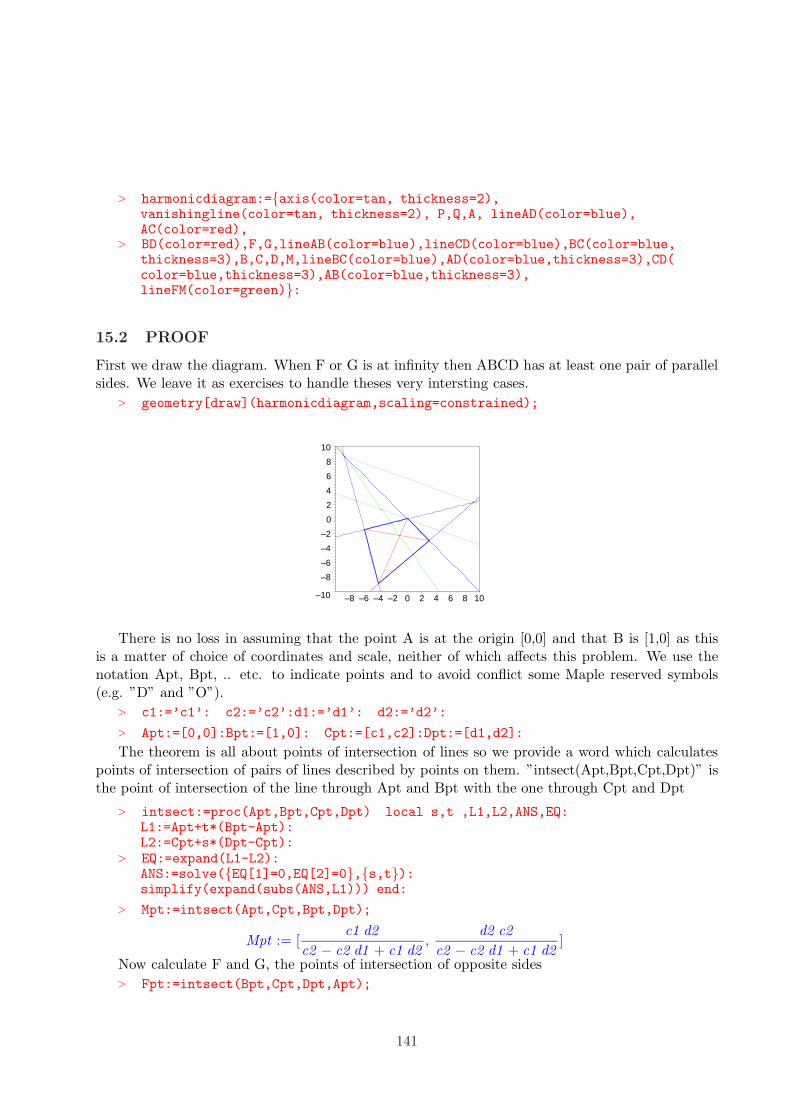
> harmonicdiagram:={axis(color=tan, thickness=2),vanishingline(color=tan, thickness=2), P,Q,A, lineAD(color=blue),AC(color=red),

> BD(color=red),F,G,lineAB(color=blue),lineCD(color=blue),BC(color=blue,thickness=3),B,C,D,M,lineBC(color=blue),AD(color=blue,thickness=3),CD(color=blue,thickness=3),AB(color=blue,thickness=3),lineFM(color=green)}:

15.2 PROOF

First we draw the diagram. When F or G is at infinity then ABCD has at least one pair of parallelsides. We leave it as exercises to handle theses very intersting cases.

> geometry[draw](harmonicdiagram,scaling=constrained);

–10

–8

–6

–4

–2

0

2

4

6

8

10

–8 –6 –4 –2 0 2 4 6 8 10

There is no loss in assuming that the point A is at the origin [0,0] and that B is [1,0] as thisis a matter of choice of coordinates and scale, neither of which affects this problem. We use thenotation Apt, Bpt, .. etc. to indicate points and to avoid conflict some Maple reserved symbols(e.g. ”D” and ”O”).

> c1:=’c1’: c2:=’c2’:d1:=’d1’: d2:=’d2’:

> Apt:=[0,0]:Bpt:=[1,0]: Cpt:=[c1,c2]:Dpt:=[d1,d2]:

The theorem is all about points of intersection of lines so we provide a word which calculatespoints of intersection of pairs of lines described by points on them. ”intsect(Apt,Bpt,Cpt,Dpt)” isthe point of intersection of the line through Apt and Bpt with the one through Cpt and Dpt

> intsect:=proc(Apt,Bpt,Cpt,Dpt) local s,t ,L1,L2,ANS,EQ:L1:=Apt+t*(Bpt-Apt):L2:=Cpt+s*(Dpt-Cpt):

> EQ:=expand(L1-L2):ANS:=solve({EQ[1]=0,EQ[2]=0},{s,t}):simplify(expand(subs(ANS,L1))) end:

> Mpt:=intsect(Apt,Cpt,Bpt,Dpt);

Mpt := [c1 d2

c2 − c2 d1 + c1 d2,

d2 c2

c2 − c2 d1 + c1 d2]

Now calculate F and G, the points of intersection of opposite sides> Fpt:=intsect(Bpt,Cpt,Dpt,Apt);

141

Fpt := [− c2 d1

−d2 + c1 d2 − c2 d1, − c2 d2

−d2 + c1 d2 − c2 d1]

> Gpt:=intsect(Apt,Bpt,Cpt,Dpt);

Gpt := [−−c2 d1 + c1 d2

c2 − d2, 0]

The line parallel to the line through F and G which passes through A has parametric formA+t(F -G). With t=1 we have a point other than A on this line

> Tpt:=Apt+(Fpt-Gpt);

Tpt := [−c2 d1 + c1 d2

c2 − d2− c2 d1

−d2 + c1 d2 − c2 d1, − c2 d2

−d2 + c1 d2 − c2 d1]

Now we calculate P and Q, the points of intersection of this parallel with the lines BC and MF> Ppt:=intsect(Bpt,Cpt,Apt,Tpt);

Ppt := [(2 d2 c2 d1 − 2 d1 c2 c1 d2 + d1 2 c2 2 − c1 d2 2 + c1 2 d2 2 − c2 2 d1 )/(c1 2 d2 2

− 2 c1 d2 2 − 2 d1 c2 c1 d2 + c2 c1 d2 + d2 2 + 2 d2 c2 d1 − d2 c2 − c2 2 d1

+ d1 2 c2 2),−d2 c2 (c2 − d2 )/(c1 2 d2 2 − 2 c1 d2 2 − 2 d1 c2 c1 d2 + c2 c1 d2 + d2 2

+ 2 d2 c2 d1 − d2 c2 − c2 2 d1 + d1 2 c2 2)]> Qpt:=intsect(Mpt,Fpt,Apt,Tpt);

Qpt := [2 d2 c2 d1 − 2 d1 c2 c1 d2 + d1 2 c2 2 − c1 d2 2 + c1 2 d2 2 − c2 2 d1

2 (−d2 + c1 d2 − c2 d1 ) (c2 − d2 + c1 d2 − c2 d1 ),

− (c2 − d2 ) d2 c2

2 (−d2 + c1 d2 − c2 d1 ) (c2 − d2 + c1 d2 − c2 d1 )]

The theorem says that the distance from P to Q is equal to the distance from Q to A. Sincewe have set A to be the origin this is equivalent to saying that the distance from P to the originis twice the distance from Q to the origin which is equivalent to ”ratsq” the ratio of the squaresbeing 4.

> ratsq:=(Ppt[1]^2+Ppt[2]^2)/(Qpt[1]^2+Qpt[2]^2);

ratsq := ((2 d2 c2 d1 − 2 d1 c2 c1 d2 + d1 2 c2 2 − c1 d2 2 + c1 2 d2 2 − c2 2 d1 )2/

(c1 2 d2 2

− 2 c1 d2 2 − 2 d1 c2 c1 d2 + c2 c1 d2 + d2 2 + 2 d2 c2 d1 − d2 c2 − c2 2 d1

+ d1 2 c2 2)2 + d2 2 c2 2 (c2 − d2 )2/

(c1 2 d2 2 − 2 c1 d2 2 − 2 d1 c2 c1 d2 + c2 c1 d2

+ d2 2 + 2 d2 c2 d1 − d2 c2 − c2 2 d1 + d1 2 c2 2)2)/

(

(2 d2 c2 d1 − 2 d1 c2 c1 d2 + d1 2 c2 2 − c1 d2 2 + c1 2 d2 2 − c2 2 d1 )2

4 (−d2 + c1 d2 − c2 d1 )2 (c2 − d2 + c1 d2 − c2 d1 )2

+(c2 − d2 )2 d2 2 c2 2

4 (−d2 + c1 d2 − c2 d1 )2 (c2 − d2 + c1 d2 − c2 d1 )2)

> simplify(expand(ratsq));

4

This completes the proof.

142

15.3 Exercises

1. Explain why statement of the harmonic ray theorem if F and G are points at infinity the theoremshould be interpreted as assuming that the quadrilateral is a rectangle. Prove the theoem in thiscase (Maple is not required)

2. Interpret the harmonic ray theorem when G is a point at infinity and F is not. Prove thetheorem in this case (Maple is not required)

3. Check the necessity of the hypothesis that L be parallel to the line FG by doing the calcu-lations for the harmonic ray theorem in a case when L is not parallel to the line FG.

143

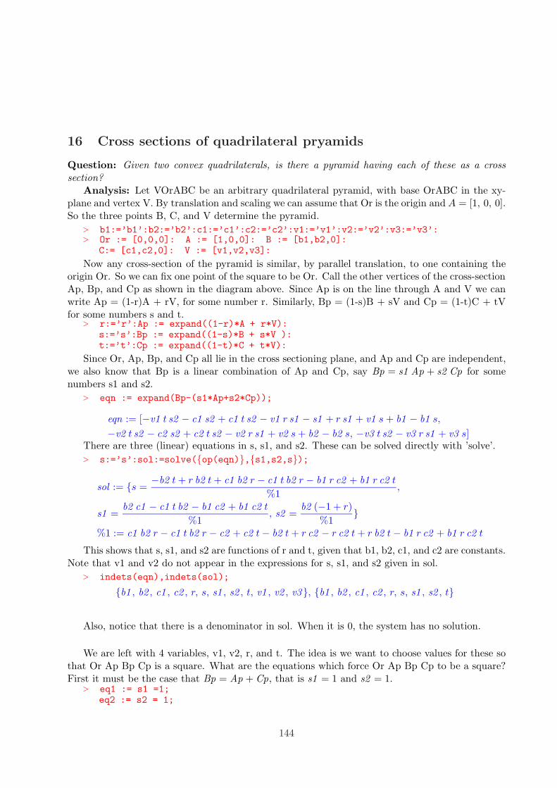
16 Cross sections of quadrilateral pryamids

Question: Given two convex quadrilaterals, is there a pyramid having each of these as a crosssection?

Analysis: Let VOrABC be an arbitrary quadrilateral pyramid, with base OrABC in the xy-plane and vertex V. By translation and scaling we can assume that Or is the origin and A = [1, 0, 0].So the three points B, C, and V determine the pyramid.

> b1:=’b1’:b2:=’b2’:c1:=’c1’:c2:=’c2’:v1:=’v1’:v2:=’v2’:v3:=’v3’:> Or := [0,0,0]: A := [1,0,0]: B := [b1,b2,0]:

C:= [c1,c2,0]: V := [v1,v2,v3]:

Now any cross-section of the pyramid is similar, by parallel translation, to one containing theorigin Or. So we can fix one point of the square to be Or. Call the other vertices of the cross-sectionAp, Bp, and Cp as shown in the diagram above. Since Ap is on the line through A and V we canwrite Ap = (1-r)A + rV, for some number r. Similarly, Bp = (1-s)B + sV and Cp = (1-t)C + tVfor some numbers s and t.

> r:=’r’:Ap := expand((1-r)*A + r*V):s:=’s’:Bp := expand((1-s)*B + s*V ):t:=’t’:Cp := expand((1-t)*C + t*V):

Since Or, Ap, Bp, and Cp all lie in the cross sectioning plane, and Ap and Cp are independent,we also know that Bp is a linear combination of Ap and Cp, say Bp = s1 Ap + s2 Cp for somenumbers s1 and s2.

> eqn := expand(Bp-(s1*Ap+s2*Cp));

eqn := [−v1 t s2 − c1 s2 + c1 t s2 − v1 r s1 − s1 + r s1 + v1 s + b1 − b1 s,

−v2 t s2 − c2 s2 + c2 t s2 − v2 r s1 + v2 s + b2 − b2 s, −v3 t s2 − v3 r s1 + v3 s]There are three (linear) equations in s, s1, and s2. These can be solved directly with ’solve’.> s:=’s’:sol:=solve({op(eqn)},{s1,s2,s});

sol := {s =−b2 t + r b2 t + c1 b2 r − c1 t b2 r − b1 r c2 + b1 r c2 t

%1,

s1 =b2 c1 − c1 t b2 − b1 c2 + b1 c2 t

%1, s2 =

b2 (−1 + r)

%1}

%1 := c1 b2 r − c1 t b2 r − c2 + c2 t − b2 t + r c2 − r c2 t + r b2 t − b1 r c2 + b1 r c2 t

This shows that s, s1, and s2 are functions of r and t, given that b1, b2, c1, and c2 are constants.Note that v1 and v2 do not appear in the expressions for s, s1, and s2 given in sol.

> indets(eqn),indets(sol);

{b1 , b2 , c1 , c2 , r, s, s1 , s2 , t, v1 , v2 , v3}, {b1 , b2 , c1 , c2 , r, s, s1 , s2 , t}

Also, notice that there is a denominator in sol. When it is 0, the system has no solution.

We are left with 4 variables, v1, v2, r, and t. The idea is we want to choose values for these sothat Or Ap Bp Cp is a square. What are the equations which force Or Ap Bp Cp to be a square?First it must be the case that Bp = Ap + Cp, that is s1 = 1 and s2 = 1.

> eq1 := s1 =1;eq2 := s2 = 1;

144

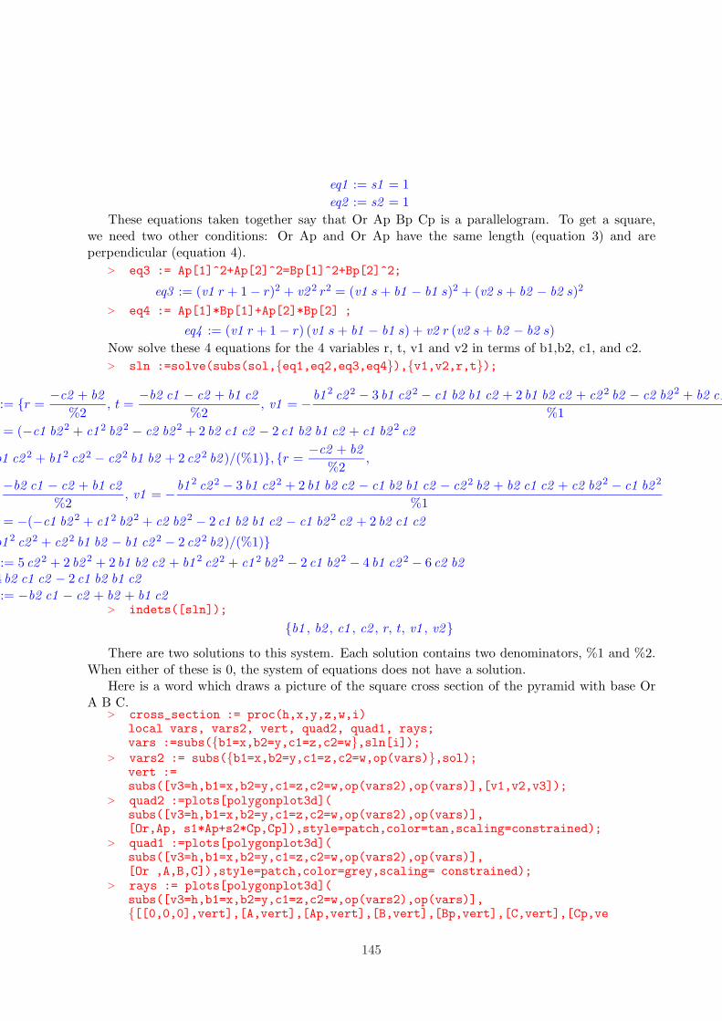
eq1 := s1 = 1

eq2 := s2 = 1

These equations taken together say that Or Ap Bp Cp is a parallelogram. To get a square,we need two other conditions: Or Ap and Or Ap have the same length (equation 3) and areperpendicular (equation 4).

> eq3 := Ap[1]^2+Ap[2]^2=Bp[1]^2+Bp[2]^2;

eq3 := (v1 r + 1 − r)2 + v2 2 r2 = (v1 s + b1 − b1 s)2 + (v2 s + b2 − b2 s)2

> eq4 := Ap[1]*Bp[1]+Ap[2]*Bp[2] ;

eq4 := (v1 r + 1 − r) (v1 s + b1 − b1 s) + v2 r (v2 s + b2 − b2 s)

Now solve these 4 equations for the 4 variables r, t, v1 and v2 in terms of b1,b2, c1, and c2.> sln :=solve(subs(sol,{eq1,eq2,eq3,eq4}),{v1,v2,r,t});

sln := {r =−c2 + b2

%2, t =

−b2 c1 − c2 + b1 c2

%2, v1 = −b1 2 c2 2 − 3 b1 c2 2 − c1 b2 b1 c2 + 2 b1 b2 c2 + c2 2 b2 − c2 b2 2 + b2 c1

%1

v2 = (−c1 b2 2 + c1 2 b2 2 − c2 b2 2 + 2 b2 c1 c2 − 2 c1 b2 b1 c2 + c1 b2 2 c2

b1 c2 2 + b1 2 c2 2 − c2 2 b1 b2 + 2 c2 2 b2 )/(%1)}, {r =−c2 + b2

%2,

=−b2 c1 − c2 + b1 c2

%2, v1 = −b1 2 c2 2 − 3 b1 c2 2 + 2 b1 b2 c2 − c1 b2 b1 c2 − c2 2 b2 + b2 c1 c2 + c2 b2 2 − c1 b2 2

%1

v2 = −(−c1 b2 2 + c1 2 b2 2 + c2 b2 2 − 2 c1 b2 b1 c2 − c1 b2 2 c2 + 2 b2 c1 c2

b1 2 c2 2 + c2 2 b1 b2 − b1 c2 2 − 2 c2 2 b2 )/(%1)}%1 := 5 c2 2 + 2 b2 2 + 2 b1 b2 c2 + b1 2 c2 2 + c1 2 b2 2 − 2 c1 b2 2 − 4 b1 c2 2 − 6 c2 b2

4 b2 c1 c2 − 2 c1 b2 b1 c2

%2 := −b2 c1 − c2 + b2 + b1 c2> indets([sln]);

{b1 , b2 , c1 , c2 , r, t, v1 , v2}

There are two solutions to this system. Each solution contains two denominators, %1 and %2.When either of these is 0, the system of equations does not have a solution.

Here is a word which draws a picture of the square cross section of the pyramid with base OrA B C.

> cross_section := proc(h,x,y,z,w,i)local vars, vars2, vert, quad2, quad1, rays;vars :=subs({b1=x,b2=y,c1=z,c2=w},sln[i]);

> vars2 := subs({b1=x,b2=y,c1=z,c2=w,op(vars)},sol);vert :=subs([v3=h,b1=x,b2=y,c1=z,c2=w,op(vars2),op(vars)],[v1,v2,v3]);

> quad2 :=plots[polygonplot3d](subs([v3=h,b1=x,b2=y,c1=z,c2=w,op(vars2),op(vars)],[Or,Ap, s1*Ap+s2*Cp,Cp]),style=patch,color=tan,scaling=constrained);

> quad1 :=plots[polygonplot3d](subs([v3=h,b1=x,b2=y,c1=z,c2=w,op(vars2),op(vars)],[Or ,A,B,C]),style=patch,color=grey,scaling= constrained);

> rays := plots[polygonplot3d](subs([v3=h,b1=x,b2=y,c1=z,c2=w,op(vars2),op(vars)],{[[0,0,0],vert],[A,vert],[Ap,vert],[B,vert],[Bp,vert],[C,vert],[Cp,ve

145

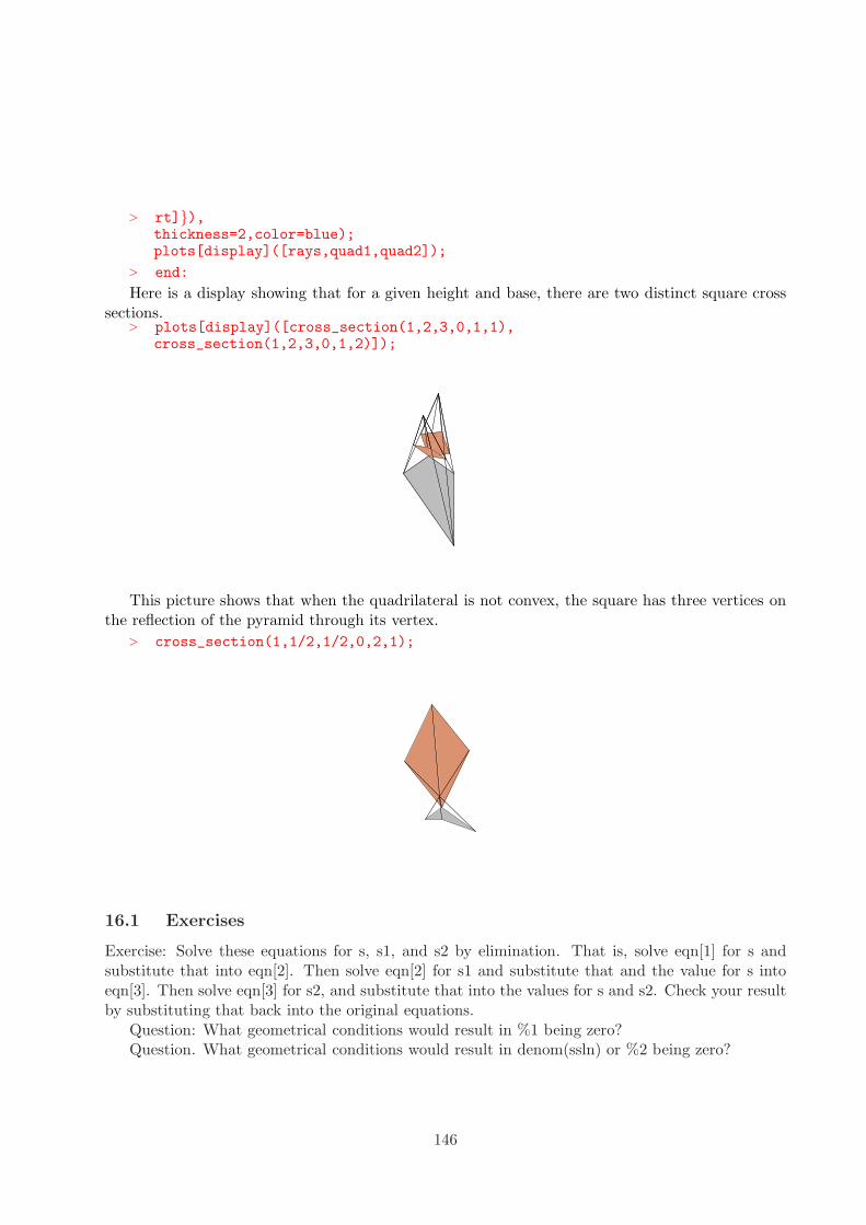
> rt]}),thickness=2,color=blue);plots[display]([rays,quad1,quad2]);

> end:

Here is a display showing that for a given height and base, there are two distinct square crosssections.

> plots[display]([cross_section(1,2,3,0,1,1),cross_section(1,2,3,0,1,2)]);

This picture shows that when the quadrilateral is not convex, the square has three vertices onthe reflection of the pyramid through its vertex.

> cross_section(1,1/2,1/2,0,2,1);

16.1 Exercises

Exercise: Solve these equations for s, s1, and s2 by elimination. That is, solve eqn[1] for s andsubstitute that into eqn[2]. Then solve eqn[2] for s1 and substitute that and the value for s intoeqn[3]. Then solve eqn[3] for s2, and substitute that into the values for s and s2. Check your resultby substituting that back into the original equations.

Question: What geometrical conditions would result in %1 being zero?Question. What geometrical conditions would result in denom(ssln) or %2 being zero?

146

17 Mirrors: More Problems from Nature

17.1 Discussion.

What do you see when you look at something in a mirror? You see the mirror image of it!Mathematically, the object is reflected in the plane of the mirror. It is an interesting problemto draw the reflection of an object in a Maple worksheet. Just how would you do that? Forexample, in the diagram below, P is a point on the object you are looking at in the mirror. How doyou determine the point Q that your eye sees when you look at the reflection of P in the mirror?The answer is that Q is the point on the mirror which also lies on the line from R (the location ofyour eye) to P’, the reflection of P through the mirror. P’ is defined mathematically as the pointon the opposite side of the mirror such that the segment PP’ is perpedicular to the mirror andis bisected by the mirror. So the point Q is a convex combination of P’ and R. The equation isQ = s R + (1 − s)P ′. If we take the plane of the mirror to be the xz-plane (y=0), then we candetermine s by solving the equation in the second coordinate (indicated by a ”2” subscript).

0 = Q2 = s R2 + (1 − s)P2′

or s = −P2′

R2 − P2′

Since P2′ = −P2, the reflection of P2 in the yz plane, we have that s = P2

R2 + P2.

17.1.1 Diagram ”light1”

> miror:=plots[polygonplot3d]([[-2,0,0],[2,0,0],[2,0,3],[-2,0,3]],style=wireframe,thickness=3,color=blue):flor:=plots[polygonplot3d]([[-2,-1,0],[2,-1,0],[2,1,0],[-2,1,0]],

> style=patch,thickness=3,color=tan):pointP:=plots[textplot3d]([-1,1,1,‘ P‘], font=[TIMES,BOLD,24]):refP:=plots[textplot3d]([-1,-1,1,‘ P’‘],

> font=[TIMES,BOLD,24]):plots[display]([miror,flor,pointP,refP]):eye:=plots[textplot3d]([2,2,1,‘ eye‘], font=[TIMES,BOLD,24]):P_refP:=plots[polygonplot3d]([[-1,1,1],[-1,-1,1]],

> style=wireframe,color=red):eye_refP:=plots[polygonplot3d]([[2,2,1],[-1,-1,1]],style=wireframe,color=red):

> pointQ:=plots[textplot3d]([0,0,1,‘ Q‘], font=[TIMES,BOLD,24]):light1:=plots[display]([miror,flor,pointP,refP,eye,P_refP,eye_refP,pointQ],orientation=[40,60]):

> light1;

147

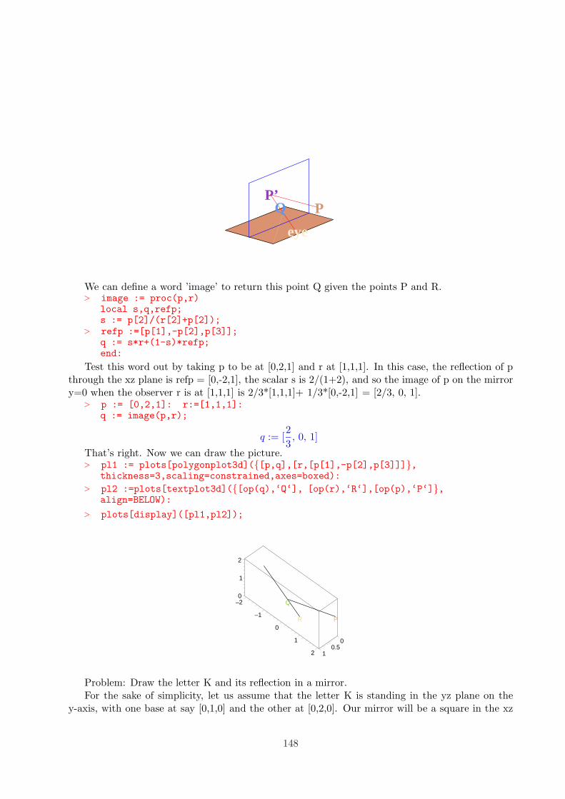
eye

P Q P’

We can define a word ’image’ to return this point Q given the points P and R.> image := proc(p,r)

local s,q,refp;s := p[2]/(r[2]+p[2]);

> refp :=[p[1],-p[2],p[3]];q := s*r+(1-s)*refp;end:

Test this word out by taking p to be at [0,2,1] and r at [1,1,1]. In this case, the reflection of pthrough the xz plane is refp = [0,-2,1], the scalar s is 2/(1+2), and so the image of p on the mirrory=0 when the observer r is at [1,1,1] is 2/3*[1,1,1]+ 1/3*[0,-2,1] = [2/3, 0, 1].

> p := [0,2,1]: r:=[1,1,1]:q := image(p,r);

q := [2

3, 0, 1]

That’s right. Now we can draw the picture.> pl1 := plots[polygonplot3d]({[p,q],[r,[p[1],-p[2],p[3]]]},

thickness=3,scaling=constrained,axes=boxed):

> pl2 :=plots[textplot3d]({[op(q),‘Q‘], [op(r),‘R‘],[op(p),‘P‘]},align=BELOW):

> plots[display]([pl1,pl2]);

Q

R P

00.5

1

–2

–1

0

1

2

0

1

2

Problem: Draw the letter K and its reflection in a mirror.For the sake of simplicity, let us assume that the letter K is standing in the yz plane on the

y-axis, with one base at say [0,1,0] and the other at [0,2,0]. Our mirror will be a square in the xz

148

plane with base [[0,0,0],[2,0,0]]. We, the observer will be standing at a point (a,b,c) to be determinedlater.

First define the mirror and the letter k.

> mir := [[0,0,0],[2,0,0],[2,0,2],[0,0,2]];

mir := [[0, 0, 0], [2, 0, 0], [2, 0, 2], [0, 0, 2]]

> mirror := plots[polygonplot3d](mir,style=patch,color=gray):> kay := [[0,1,0],[0,1,1]],[[0,1,.5],[0,1.5,1]],

[[0,1,.5],[0,1.5,0]];

kay := [[0, 1, 0], [0, 1, 1]], [[0, 1, 0.5], [0, 1.5, 1]], [[0, 1, 0.5], [0, 1.5, 0]]

> ka :=plots[polygonplot3d]({kay},thickness=3,color=red):Now the image of the letter k in the mirror is a function of the position (a,b,c) of the observer.> refkay := proc(a,b,c)

local i;seq(map(image,kay[i],[a,b,c]),i=1..nops([kay]));end:

So let’s pick an observation point ob

> ob := [2,3,1];

ob := [2, 3, 1]

obs is a blue stick located at the observation point.> obs :=

plots[polygonplot3d]([ob,[ob[1],ob[2],0]],color=blue,thickness=3):

reka is the image of the letter k in the mirror from the observation point ob.> reka :=plots[polygonplot3d]({refkay(op(ob))},thickness=3,

color=red):

We can see what this looks like with display.> plots[display]([obs,mirror,ka,reka],scaling=constrained,axes=boxed);

00.5

11.5

2

00.5

11.5

22.5

3

0

1

2

Looks fine. Copy down the input cells from above to make a word to draw the mirror, theletter, and its image in the mirror as seen from the observer.

> mirimage := proc(ob)local obs, reka;obs :=

149

> plots[polygonplot3d]([ob,[ob[1],ob[2],0]],color=blue,thickness=3):reka :=plots[polygonplot3d]({refkay(op(ob))},thickness=3,color=red):plots[display]([obs,mirror,ka,reka],scaling=constrained,axes=boxed);end:

> mirimage([3, 4,.2]);

00.5

11.5

22.5

3

0

1

2

3

4

0

1

2

Exercise: Make a movie showing what happens to the reflection as we move the observer aroundin a circle .

> movie := [seq(mirimage([2+cos(j*Pi/5),2+sin(Pi*j/5),1]),j=1..10)]:

> display(movie,insequence=true);

00.5

11.5

22.5

3

00.5

11.5

22.5

1

2

17.2 Questions:

1 Suppose we had another mirror in a vertical plane perpendicular with the first mirror with itsbase on the segment [[3,1,0],[3,3,0]]. If an observer at [2,2,1] looked in the second mirror, whatwould he see (besides himself)? Model this.

2 If you have two perfect mirrors, and hold them just right, you can see down an infinite corridor.Even with two good mirrors, you can see a large number of reflections of reflections. Observe thisand describe what you see exactly. As an experiment, hold up a transparency with a letter kwritten on it. How hard would this be to model?

3 If you have three mirrors which form a corner of a box and shine a beam of light almost intothe corner, what happens to the beam?

150

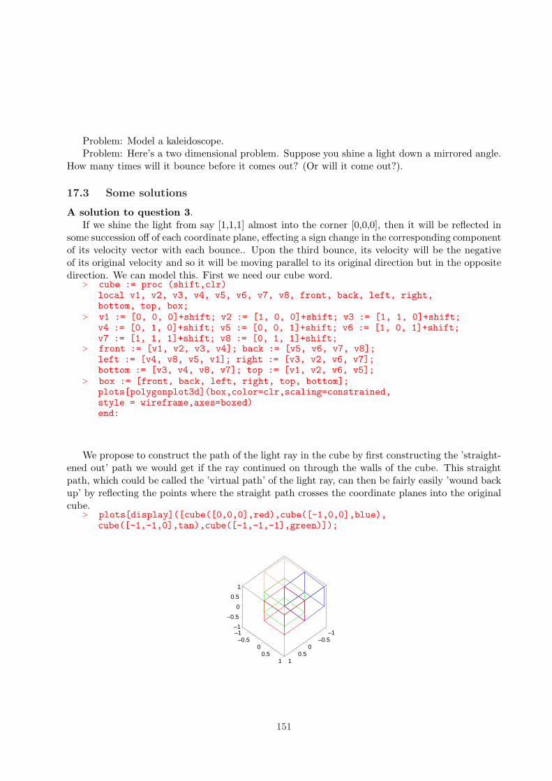
Problem: Model a kaleidoscope.Problem: Here’s a two dimensional problem. Suppose you shine a light down a mirrored angle.

How many times will it bounce before it comes out? (Or will it come out?).

17.3 Some solutions

A solution to question 3.If we shine the light from say [1,1,1] almost into the corner [0,0,0], then it will be reflected in

some succession off of each coordinate plane, effecting a sign change in the corresponding componentof its velocity vector with each bounce.. Upon the third bounce, its velocity will be the negativeof its original velocity and so it will be moving parallel to its original direction but in the oppositedirection. We can model this. First we need our cube word.

> cube := proc (shift,clr)local v1, v2, v3, v4, v5, v6, v7, v8, front, back, left, right,bottom, top, box;



> box := [front, back, left, right, top, bottom];plots[polygonplot3d](box,color=clr,scaling=constrained,style = wireframe,axes=boxed)end:

We propose to construct the path of the light ray in the cube by first constructing the ’straight-ened out’ path we would get if the ray continued on through the walls of the cube. This straightpath, which could be called the ’virtual path’ of the light ray, can then be fairly easily ’wound backup’ by reflecting the points where the straight path crosses the coordinate planes into the originalcube.

> plots[display]([cube([0,0,0],red),cube([-1,0,0],blue),cube([-1,-1,0],tan),cube([-1,-1,-1],green)]);

–1–0.5

00.5

1

–1–0.5

00.5

1

–1

–0.5

0

0.5

1

151

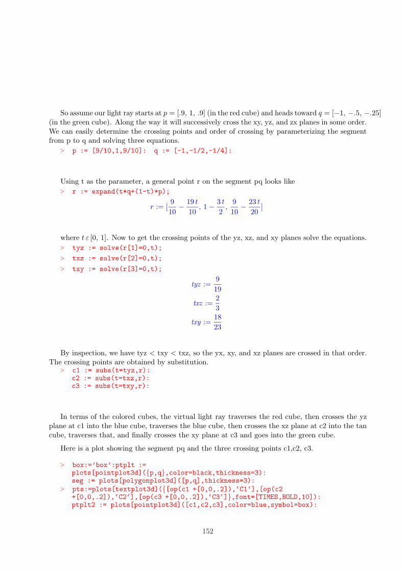
So assume our light ray starts at p = [.9, 1, .9] (in the red cube) and heads toward q = [−1, −.5, −.25](in the green cube). Along the way it will successively cross the xy, yz, and zx planes in some order.We can easily determine the crossing points and order of crossing by parameterizing the segmentfrom p to q and solving three equations.

> p := [9/10,1,9/10]: q := [-1,-1/2,-1/4]:

Using t as the parameter, a general point r on the segment pq looks like> r := expand(t*q+(1-t)*p);

r := [9

10− 19 t

10, 1 − 3 t

2,

9

10− 23 t

20]

where t ε [0, 1]. Now to get the crossing points of the yz, xz, and xy planes solve the equations.

> tyz := solve(r[1]=0,t);

> txz := solve(r[2]=0,t);

> txy := solve(r[3]=0,t);

tyz :=9

19

txz :=2

3

txy :=18

23

By inspection, we have tyz < txy < txz, so the yx, xy, and xz planes are crossed in that order.The crossing points are obtained by substitution.

> c1 := subs(t=tyz,r):c2 := subs(t=txz,r):c3 := subs(t=txy,r):

In terms of the colored cubes, the virtual light ray traverses the red cube, then crosses the yzplane at c1 into the blue cube, traverses the blue cube, then crosses the xz plane at c2 into the tancube, traverses that, and finally crosses the xy plane at c3 and goes into the green cube.

Here is a plot showing the segment pq and the three crossing points c1,c2, c3.

> box:=’box’:ptplt :=plots[pointplot3d]({p,q},color=black,thickness=3):seg := plots[polygonplot3d]([p,q],thickness=3):

> pts:=plots[textplot3d]({[op(c1 +[0,0,.2]),‘C1‘],[op(c2+[0,0,.2]),‘C2‘],[op(c3 +[0,0,.2]),‘C3‘]},font=[TIMES,BOLD,10]):ptplt2 := plots[pointplot3d]([c1,c2,c3],color=blue,symbol=box):

152

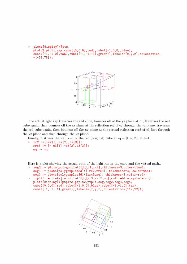
> plots[display]([pts,ptplt2,ptplt,seg,cube([0,0,0],red),cube([-1,0,0],blue),cube([-1,-1,0],tan),cube([-1,-1,-1],green)],labels=[x,y,z],orientation=[-58,78]);

C2C3

C1

–1 –0.5 0 0.5 16 –0.50 0.5 1

y

–1

–0.5

0

0.5

1

z

The actual light ray traverses the red cube, bounces off of the yz plane at c1, traverses the redcube again, then bounces off the xz plane at the reflection rc2 of c2 through the yz plane, traversesthe red cube again, then bounces off the xy plane at the second reflection rrc3 of c3 first throughthe yz plane and then through the xz plane.

Finally, it strikes the wall x=1 of the red (original) cube at -q = [1,.5,.25] at t=1.> rc2 :=[-c2[1],c2[2],c2[3]]:

rrc3 := [- c3[1],-c3[2],c3[3]]:mq := -q:

Here is a plot showing the actual path of the light ray in the cube and the virtual path..> seg2 := plots[polygonplot3d]([c1,rc2],thickness=3,color=blue):

seg3 := plots[polygonplot3d]([ rc2,rrc3], thickness=3, color=tan):seg4 := plots[polygonplot3d]([rrc3,mq], thickness=3,color=red):

> ptplt3 := plots[pointplot3d]([rc2,rrc3,mq],color=blue,symbol=box):plots[display]([ptplt3,ptplt2,ptplt,seg,seg2,seg3,seg4,cube([0,0,0],red),cube([-1,0,0],blue),cube([-1,-1,0],tan),cube([-1,-1,-1],green)],labels=[x,y,z],orientation=[117,22]);

–1–0.5

00.5

1

6

–1

–0.5

0

0.5

1

y–1

0

1

z

153

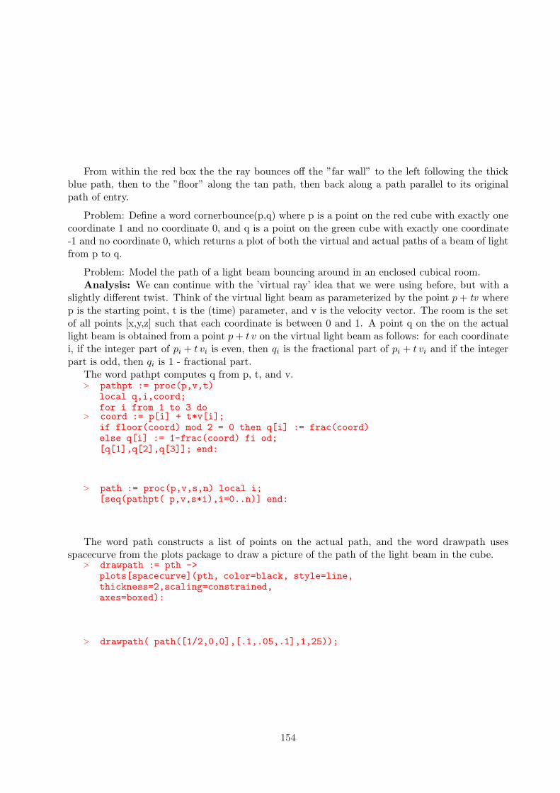
From within the red box the the ray bounces off the ”far wall” to the left following the thickblue path, then to the ”floor” along the tan path, then back along a path parallel to its originalpath of entry.

Problem: Define a word cornerbounce(p,q) where p is a point on the red cube with exactly onecoordinate 1 and no coordinate 0, and q is a point on the green cube with exactly one coordinate-1 and no coordinate 0, which returns a plot of both the virtual and actual paths of a beam of lightfrom p to q.

Problem: Model the path of a light beam bouncing around in an enclosed cubical room.Analysis: We can continue with the ’virtual ray’ idea that we were using before, but with a

slightly different twist. Think of the virtual light beam as parameterized by the point p + tv wherep is the starting point, t is the (time) parameter, and v is the velocity vector. The room is the setof all points [x,y,z] such that each coordinate is between 0 and 1. A point q on the on the actuallight beam is obtained from a point p + t v on the virtual light beam as follows: for each coordinatei, if the integer part of pi + t vi is even, then qi is the fractional part of pi + t vi and if the integerpart is odd, then qi is 1 - fractional part.

The word pathpt computes q from p, t, and v.> pathpt := proc(p,v,t)

local q,i,coord;for i from 1 to 3 do

> coord := p[i] + t*v[i];if floor(coord) mod 2 = 0 then q[i] := frac(coord)else q[i] := 1-frac(coord) fi od;[q[1],q[2],q[3]]; end:

> path := proc(p,v,s,n) local i;[seq(pathpt( p,v,s*i),i=0..n)] end:

The word path constructs a list of points on the actual path, and the word drawpath usesspacecurve from the plots package to draw a picture of the path of the light beam in the cube.

> drawpath := pth ->plots[spacecurve](pth, color=black, style=line,thickness=2,scaling=constrained,axes=boxed):

> drawpath( path([1/2,0,0],[.1,.05,.1],1,25));

154

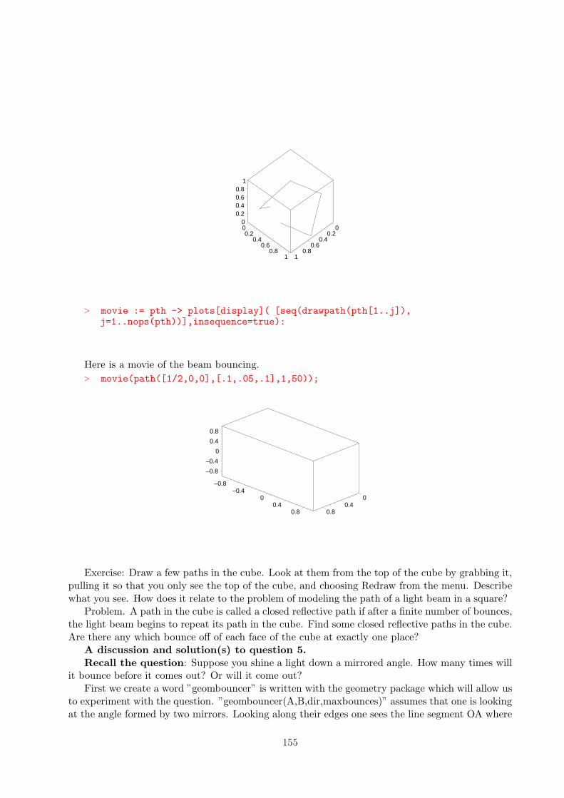
00.2

0.40.6

0.81

00.2

0.40.6

0.81

00.20.40.60.8

1

> movie := pth -> plots[display]( [seq(drawpath(pth[1..j]),j=1..nops(pth))],insequence=true):

Here is a movie of the beam bouncing.> movie(path([1/2,0,0],[.1,.05,.1],1,50));

00.4

0.8

–0.8–0.4

00.4

0.8

–0.8

–0.4

0

0.4

0.8

Exercise: Draw a few paths in the cube. Look at them from the top of the cube by grabbing it,pulling it so that you only see the top of the cube, and choosing Redraw from the menu. Describewhat you see. How does it relate to the problem of modeling the path of a light beam in a square?

Problem. A path in the cube is called a closed reflective path if after a finite number of bounces,the light beam begins to repeat its path in the cube. Find some closed reflective paths in the cube.Are there any which bounce off of each face of the cube at exactly one place?

A discussion and solution(s) to question 5.Recall the question: Suppose you shine a light down a mirrored angle. How many times will

it bounce before it comes out? Or will it come out?First we create a word ”geombouncer” is written with the geometry package which will allow us

to experiment with the question. ”geombouncer(A,B,dir,maxbounces)” assumes that one is lookingat the angle formed by two mirrors. Looking along their edges one sees the line segment OA where

155

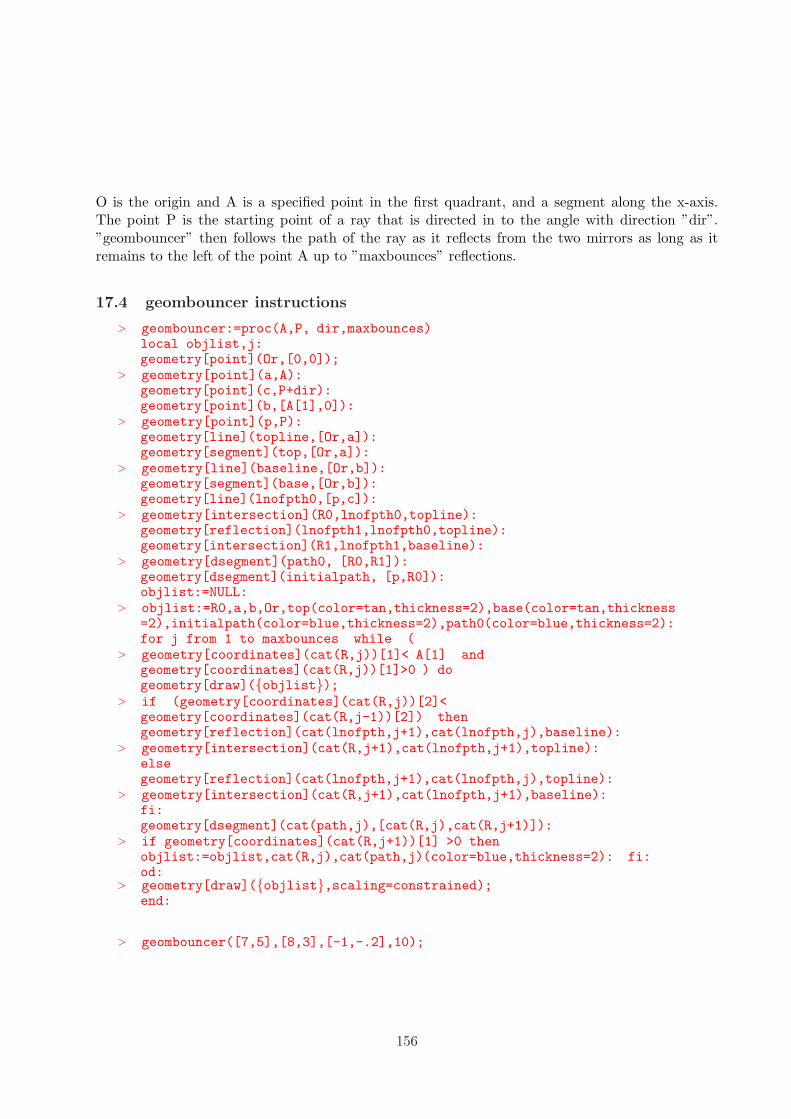
O is the origin and A is a specified point in the first quadrant, and a segment along the x-axis.The point P is the starting point of a ray that is directed in to the angle with direction ”dir”.”geombouncer” then follows the path of the ray as it reflects from the two mirrors as long as itremains to the left of the point A up to ”maxbounces” reflections.

17.4 geombouncer instructions

> geombouncer:=proc(A,P, dir,maxbounces)local objlist,j:geometry[point](Or,[0,0]);

> geometry[point](a,A):geometry[point](c,P+dir):geometry[point](b,[A[1],0]):

> geometry[point](p,P):geometry[line](topline,[Or,a]):geometry[segment](top,[Or,a]):

> geometry[line](baseline,[Or,b]):geometry[segment](base,[Or,b]):geometry[line](lnofpth0,[p,c]):

> geometry[intersection](R0,lnofpth0,topline):geometry[reflection](lnofpth1,lnofpth0,topline):geometry[intersection](R1,lnofpth1,baseline):

> geometry[dsegment](path0, [R0,R1]):geometry[dsegment](initialpath, [p,R0]):objlist:=NULL:

> objlist:=R0,a,b,Or,top(color=tan,thickness=2),base(color=tan,thickness=2),initialpath(color=blue,thickness=2),path0(color=blue,thickness=2):for j from 1 to maxbounces while (

> geometry[coordinates](cat(R,j))[1]< A[1] andgeometry[coordinates](cat(R,j))[1]>0 ) dogeometry[draw]({objlist});

> if (geometry[coordinates](cat(R,j))[2]<geometry[coordinates](cat(R,j-1))[2]) thengeometry[reflection](cat(lnofpth,j+1),cat(lnofpth,j),baseline):

> geometry[intersection](cat(R,j+1),cat(lnofpth,j+1),topline):elsegeometry[reflection](cat(lnofpth,j+1),cat(lnofpth,j),topline):

> geometry[intersection](cat(R,j+1),cat(lnofpth,j+1),baseline):fi:geometry[dsegment](cat(path,j),[cat(R,j),cat(R,j+1)]):

> if geometry[coordinates](cat(R,j+1))[1] >0 thenobjlist:=objlist,cat(R,j),cat(path,j)(color=blue,thickness=2): fi:od:

> geometry[draw]({objlist},scaling=constrained);end:

> geombouncer([7,5],[8,3],[-1,-.2],10);

156

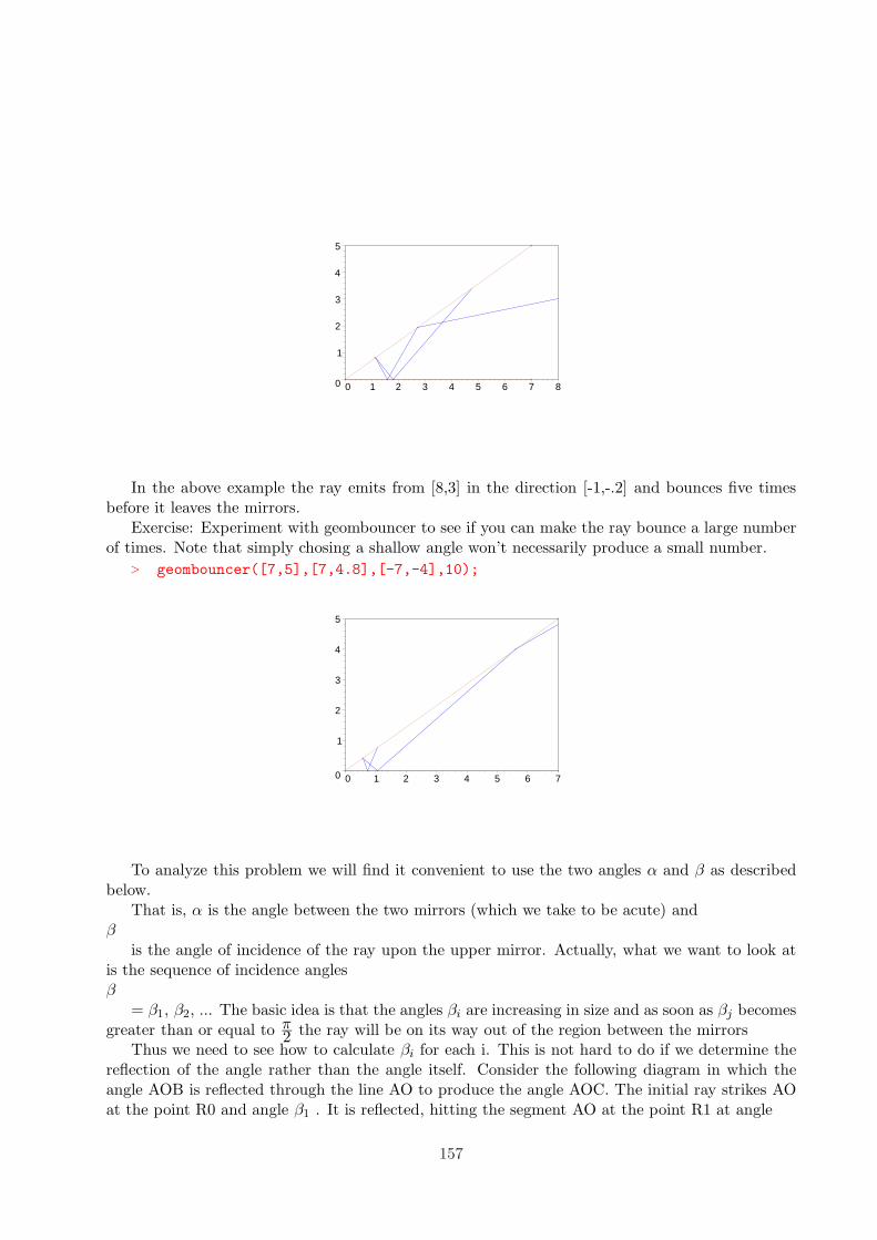
0

1

2

3

4

5

0 1 2 3 4 5 6 7 8

In the above example the ray emits from [8,3] in the direction [-1,-.2] and bounces five timesbefore it leaves the mirrors.

Exercise: Experiment with geombouncer to see if you can make the ray bounce a large numberof times. Note that simply chosing a shallow angle won’t necessarily produce a small number.

> geombouncer([7,5],[7,4.8],[-7,-4],10);

0

1

2

3

4

5

0 1 2 3 4 5 6 7

To analyze this problem we will find it convenient to use the two angles α and β as describedbelow.

That is, α is the angle between the two mirrors (which we take to be acute) andβ

is the angle of incidence of the ray upon the upper mirror. Actually, what we want to look atis the sequence of incidence anglesβ

= β1, β2, ... The basic idea is that the angles βi are increasing in size and as soon as βj becomesgreater than or equal to π

2 the ray will be on its way out of the region between the mirrorsThus we need to see how to calculate βi for each i. This is not hard to do if we determine the

reflection of the angle rather than the angle itself. Consider the following diagram in which theangle AOB is reflected through the line AO to produce the angle AOC. The initial ray strikes AOat the point R0 and angle β1 . It is reflected, hitting the segment AO at the point R1 at angle

157

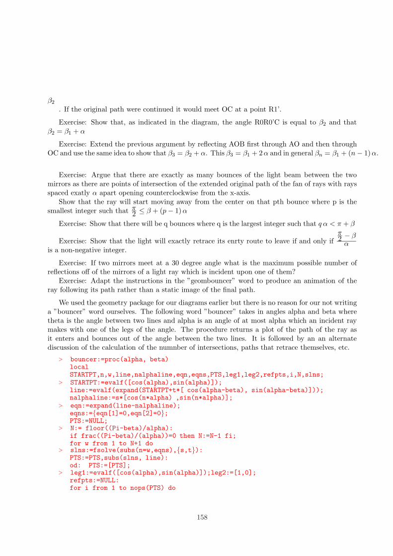
β2

. If the original path were continued it would meet OC at a point R1’.

Exercise: Show that, as indicated in the diagram, the angle R0R0’C is equal to β2 and thatβ2 = β1 + α

Exercise: Extend the previous argument by reflecting AOB first through AO and then throughOC and use the same idea to show that β3 = β2 + α. This β3 = β1 + 2α and in general βn = β1 + (n − 1)α.

Exercise: Argue that there are exactly as many bounces of the light beam between the twomirrors as there are points of intersection of the extended original path of the fan of rays with raysspaced exatly α apart opening counterclockwise from the x-axis.

Show that the ray will start moving away from the center on that pth bounce where p is thesmallest integer such that π

2 ≤ β + (p − 1)α

Exercise: Show that there will be q bounces where q is the largest integer such that q α < π + β

Exercise: Show that the light will exactly retrace its enrty route to leave if and only ifπ2 − β

αis a non-negative integer.

Exercise: If two mirrors meet at a 30 degree angle what is the maximum possible number ofreflections off of the mirrors of a light ray which is incident upon one of them?

Exercise: Adapt the instructions in the ”geombouncer” word to produce an animation of theray following its path rather than a static image of the final path.

We used the geometry package for our diagrams earlier but there is no reason for our not writinga ”bouncer” word ourselves. The following word ”bouncer” takes in angles alpha and beta wheretheta is the angle between two lines and alpha is an angle of at most alpha which an incident raymakes with one of the legs of the angle. The procedure returns a plot of the path of the ray asit enters and bounces out of the angle between the two lines. It is followed by an an alternatediscussion of the calculation of the numnber of intersections, paths that retrace themselves, etc.

> bouncer:=proc(alpha, beta)localSTARTPT,n,w,line,nalphaline,eqn,eqns,PTS,leg1,leg2,refpts,i,N,slns;

> STARTPT:=evalf([cos(alpha),sin(alpha)]);line:=evalf(expand(STARTPT+t*[ cos(alpha-beta), sin(alpha-beta)]));nalphaline:=s*[cos(n*alpha) ,sin(n*alpha)];

> eqn:=expand(line-nalphaline);eqns:={eqn[1]=0,eqn[2]=0};PTS:=NULL;

> N:= floor((Pi-beta)/alpha):if frac((Pi-beta)/(alpha))=0 then N:=N-1 fi;for w from 1 to N+1 do

> slns:=fsolve(subs(n=w,eqns),{s,t}):PTS:=PTS,subs(slns, line):od: PTS:=[PTS];

> leg1:=evalf([cos(alpha),sin(alpha)]);leg2:=[1,0];refpts:=NULL:for i from 1 to nops(PTS) do

158

> if i mod 2 = 1 then refpts:=refpts,linalg[norm](PTS[i],2)*leg1; elserefpts:=refpts, linalg[norm](PTS[i],2)*leg2 fi; od:plots[display](

> [plots[polygonplot]([[0,0],[1,0],[1,tan(alpha)]],style=patch,color=tan), plot([refpts]),plots[polygonplot]([STARTPT,subs(t=.2,line),STARTPT],scaling=constrain

> ed )]):end:

> bouncer(Pi/4,Pi/8);

0

0.2

0.4

0.6

0.8

1

0.2 0.4 0.6 0.8 1

The unterminated line is the incident ray and the returning path ends at its last bounce point.That is the returning ray will reflect at an angle smaller than theta, the lower left angle of thecolored triangle and will therefore not hit either leg of the triangle again.

If α is the incident angle which is less than or equal to theta then the angle at which the rayrebounds at the ith bounce is α + i θ (where the initial bounce is the ”zeroth”). The condition forthe ray to return exactly along its original path is that it hit one of the legs at a right angle, thatis that α + n θ is a right angle

> eqn1:=beta+n*alpha=Pi/2;

eqn1 := β + n α =π

2> critbeta:=solve(eqn1,beta);

critbeta := −n α +π

2

Since β ≤ α we see that n is the integer part of π2α unless this is actually an integer in which

case this value of n is one less than π2α . The latter situation only occurs when theta has the form

π2 k where k is an integer. For the moment, we ignore this possibility and have the formula

> critbeta:=proc(alpha) Pi/2-floor(Pi/(2*alpha))*alpha end;

159

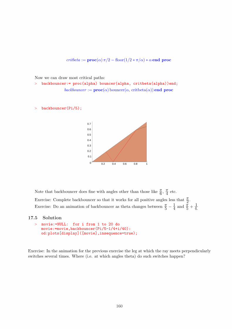
critbeta := proc(α)π/2 − floor(1/2 ∗ π/α) ∗ α end proc

Now we can draw most critical paths:> backbouncer:= proc(alpha) bouncer(alpha, critbeta(alpha))end;

backbouncer := proc(α) bouncer(α, critbeta(α)) end proc

> backbouncer(Pi/5);

0

0.1

0.2

0.3

0.4

0.5

0.6

0.7

0.2 0.4 0.6 0.8 1

Note that backbouncer does fine with angles other than those like π6 , π

4 etc.

Exercise: Complete backbouncer so that it works for all positive angles less that π2 .

Exercise: Do an animation of backbouncer as theta changes between π5 − 1

4 and π5 + 1

4.

17.5 Solution> movie:=NULL: for i from 1 to 20 do

movie:=movie,backbouncer(Pi/5-1/4+i/40):od:plots[display]([movie],insequence=true);

Exercise: In the animation for the previous exercise the leg at which the ray meets perpendicularlyswitches several times. Where (i.e. at which angles theta) do such switches happen?

160

Index

’procedurize’, 47

, 36, 38, 51

a mod b, 65assignment, 53

code , 45colon, 30components, 11

equality =, 65Exercises: Making 3d Alphabet Blocks, 38expression sequence , 50

floor. , 86for .. do ... od, 61

global variable,, 44

help(polygonplot3d);, 13

if ...then...elif.. then ...elif ...then...fi; , 66

l, 38list, 53local variables , 44

m mod 2 , 86make a movie , 78make the list to be animated , 73Maple words, 41

n-gon, 14nops (L);, 77nops (number of operands), 52NOTATION: If L is a Maple list then the nth

element of Lis L[n]—, 75NULL...., 50

op., 51

plot(sin(3*x),x=-Pi..Pi);, 10plots[display[(MOV[i], OnetoTen[i]);, 80plots[display], 58plots[display]., 38

plots[polygonplot3d], 41, 45plots[polygonplot3d]([[1,2,3],[4,1,5],[7,8,3]]);, 12plots[polygonplot], 36polygon, 14polygonplot3d , 12procedures., 42projection of X from P, 132

restart;, 36

seq, 55

T := 17;, 65the fact notwithstanding , 11

useful model for making animations , 74

Visual Problem Solving, 6Visual problem solving, 11

whattype, 51

161

Documents

Visual Problem Solving with Maple - University of Kentuckycarl/vps98/visualprobs.pdf · 2009-01-08 · Visual Problem Solving with Maple by Paul Eakin, [email protected] and Carl Eberhart,