Embed Size (px)
Citation preview

VISUAL QUALITY ASSESSMENT AT LOWER MUSKEGON WATERSHED
By
Di Lu
A THESIS
Submitted to Michigan State University
in partial fulfillment of the requirements for the degree of
MASTER OF ARTS
Environmental Design
2011
ABSTRACT
VISUAL QUALITY ASSESSMENT AT LOWER MUSKEGON WATERSHED
By
Di Lu
Planners, designers, governmental agencies, and citizens are interested in evaluating
environmental quality. However, environmental quality is often quite intangible and difficult to
be described quantitatively. Nevertheless, the hypothesis for this research is that: one can predict
landscape aesthetic qualities of the Lower Muskegon Watershed by producing a statistically
validated landscape visual quality map, meaning that a generated predictive map of visual quality
is highly concordant with real images in the watershed. To construct the predictive map, photos
were taken in the study area, their visual quality was measured with an equation developed by
Burley (1997), then matched to land-uses on the map, and thus the land-uses had a visual quality
score across the study area. With another set of photographs from the study area, the scores of
the photographs were compared with the predictions of the map, employing Kendall’s
Coefficient of Concordance. The results suggest that the predictions (land-use map based scores)
and the real photographs are in concordance and significant to a high (95%) confidence level,
which supports the hypothesis.
Key Words: Environmental Psychology, Landscape Architecture, Geography, Landscape
Planning

iii
ACKNOWLEDGEMENT
First and foremost, I am inclined to express my deep gratitude to a committee member, Prof. Jon
B. Burley, for his patience, support, and advice for my personal and academic development. He
always taught me how to conduct research, but he never pushed me to do anything. From him, I
have learned a lot, such as hard work, critical thinking, research methods, and enthusiasm for
nature. He is not only an teacher, but also a friend of mine.
I would also like to thank my advisor Dr. Pat L. Crawford and committee member Dr. Robert E.
Schutzki. Their questions and comments are always clear and inspiring for me to continue my
research.
I sincerely appreciate my parents. Thanks for all the unconditional love and financial support.
Their physical and emotional supports keep me going forward.
I appreciate the help from Sihui Wang on my photo data collection and GIS data processing.
Without her help, I could not have quickly used GIS.
I also appreciate the help from Shawn Partin for assisting me in my English writing.
I would like to express thanks to my friends and teachers who helped and supported me over the
past two years studying at Michigan State University.
iv
Table of Contents List of Tables ..................................................................................................................... v
List of Figures ................................................................................................................... vi
1. Introduction .............................................................................................................. 1
2. Literature Review ..................................................................................................... 3
2.1. The Expert Paradigm .............................................................................................. 3
2.2. The Psychophysical Paradigm ................................................................................ 6
2.3. The Cognitive Paradigm ........................................................................................ 10
2.4. The Experiential Paradigm ................................................................................... 13
2.5. Comparison of the Four Paradigms ..................................................................... 14
2.6. Mapping Visual Quality ........................................................................................ 15
3. Method .................................................................................................................... 20
3.1. Research Progress Diagram .................................................................................. 20
3.2. Study Area .............................................................................................................. 21
3.3. Collecting Data ....................................................................................................... 24
3.4. Analysis Techniques ............................................................................................... 25
4. Results ..................................................................................................................... 30
4.1. Mapping Visual Quality ........................................................................................ 30
4.2. Validating the Map ................................................................................................ 37
5. Discussion ................................................................................................................ 39
6. Limitation ................................................................................................................ 46
7. Conclusion ............................................................................................................... 49
Appendix .......................................................................................................................... 50
Bibliography .................................................................................................................... 59

v
List of Tables
Table 1: Burley’s Equation 1 ............................................................................................ 25
Table 2: Independent variables ......................................................................................... 26
Table 3: Environmental quality index ............................................................................... 27
Table 4: Visual quality score of set one and set two ......................................................... 32
Table 5: Visual quality mean scores of set one by land use ............................................. 33
Table 6: Predictive scores of set two ................................................................................ 36
Table 7: Real score and predictive score of set two .......................................................... 37

vi
List of Figures
Figure 1: Research progress diagram ................................................................................ 20
Figure 2: Geographic location of Lower Muskegon Watershed ....................................... 23
Figure 3: Land-use map of Lower Muskegon Watershed ................................................ 25
Figure 4: Locations of 131 photos at Lower Muskegon Watershed ................................. 30
Figure 5: Locations of set one ........................................................................................... 31
Figure 6: Locations of set two .......................................................................................... 31
Figure 7: A typical image of farmland .............................................................................. 34
Figure 8: A typical image of water ................................................................................... 34
Figure 9: A typical image of forest ................................................................................... 34
Figure 10: A typical image of urban savanna ................................................................... 34
Figure 11: A typical image of downtown ......................................................................... 35
Figure 12: A typical image of industry ............................................................................. 35
Figure 13: Predictive visual quality map .......................................................................... 35
Figure 14: A farmland image with a predictive score of 53.660695 ................................ 36
Figure 15: Graphs of 95% confidence tails for visual preference scores: the 95% confidence scores for Figure 5.2 (63.35648) and Figure 5.3 (80.44573) ............................................ 39
Figure 16: A typical downtown image with the score of 80.44573 .................................. 40
Figure 17: A typical farmland image with the score of 63.35648 .................................... 41
vii
Figure 18: A random farmland image with the predictive score of 53.660695 ................ 41
Figure 19: A random mixed image of urban savanna, water and forest with predictive average score of 58.9274 ................................................................................................................ 42
Figure 20: Images representing directions associated with viewsheds ............................. 45
Figure 21: A typical photo of the Grand Canyon ............................................................. 47
Figure 22: Set one NO.1 ................................................................................................... 50
Figure 23: Set one NO.2 ................................................................................................... 50
Figure 24: Set one NO.3 ................................................................................................... 50
Figure 25: Set one NO.4 ................................................................................................... 50
Figure 26: Set one NO.5 ................................................................................................... 50
Figure 27: Set one NO.6 ................................................................................................... 50
Figure 28: Set one NO.7 ................................................................................................... 50
Figure 29: Set one NO.8 ................................................................................................... 50
Figure 30: Set one NO.9 ................................................................................................... 51
Figure 31: Set one NO.10 ................................................................................................. 51
Figure 32: Set one NO.11 ................................................................................................. 51
Figure 33: Set one NO.12 ................................................................................................. 51
Figure 34: Set one NO.13 ................................................................................................. 51
Figure 35: Set one NO.14 ................................................................................................. 51

viii
Figure 36: Set one NO.15 ................................................................................................. 51
Figure 37: Set one NO.16 ................................................................................................. 51
Figure 38: Set one NO.17 ................................................................................................. 52
Figure 39: Set one NO.18 ................................................................................................. 52
Figure 40: Set one NO.19 ................................................................................................. 52
Figure 41: Set one NO.20 ................................................................................................. 52
Figure 42: Set one NO.21 ................................................................................................. 52
Figure 43: Set one NO.22 ................................................................................................. 52
Figure 44: Set one NO.23 ................................................................................................. 52
Figure 45: Set one NO.24 ................................................................................................. 52
Figure 46: Set one NO.25 ................................................................................................. 53
Figure 47: Set one NO.26 ................................................................................................. 53
Figure 48: Set one NO.27 ................................................................................................. 53
Figure 49: Set one NO.28 ................................................................................................. 53
Figure 50: Set one NO.29 ................................................................................................. 53
Figure 51: Set one NO.30 ................................................................................................. 53
Figure 52: Set two NO.1 ................................................................................................... 53
Figure 53: Set two NO.2 ................................................................................................... 53
ix
Figure 54: Set two NO.3 ................................................................................................... 54
Figure 55: Set two NO.4 ................................................................................................... 54
Figure 56: Set two NO.5 ................................................................................................... 54
Figure 57: Set two NO.6 ................................................................................................... 54
Figure 58: Set two NO.7 ................................................................................................... 54
Figure 59: Set two NO.8 ................................................................................................... 54
Figure 60: Set two NO.9 ................................................................................................... 54
Figure 61: Set two NO.10 ................................................................................................. 54
Figure 62: Set two NO.11 ................................................................................................. 55
Figure 63: Set two NO.12 ................................................................................................. 55
Figure 64: Set two NO.13 ................................................................................................. 55
Figure 65: Set two NO.14 ................................................................................................. 55
Figure 66: Set two NO.15 ................................................................................................. 55
Figure 67: Set two NO.16 ................................................................................................. 55
Figure 68: Set two NO.17 ................................................................................................. 55
Figure 69: Set two NO.18 ................................................................................................. 55
Figure 70: Set two NO.19 ................................................................................................. 56
Figure 71: Set two NO.20 ................................................................................................. 56

x
Figure 72: Set two NO.21 ................................................................................................. 56
Figure 73: Set two NO.22 ................................................................................................. 56
Figure 74: Set two NO.23 ................................................................................................. 56
Figure 75: Set two NO.24 ................................................................................................. 56
Figure 76: Set two NO.25 ................................................................................................. 56
Figure 77: Set two NO.26 ................................................................................................. 56
Figure 78: Set two NO.27 ................................................................................................. 57
Figure 79: Set two NO.28 ................................................................................................. 57
Figure 80: Set two NO.29 ................................................................................................. 57
Figure 81: Set two NO.30 ................................................................................................. 57
1
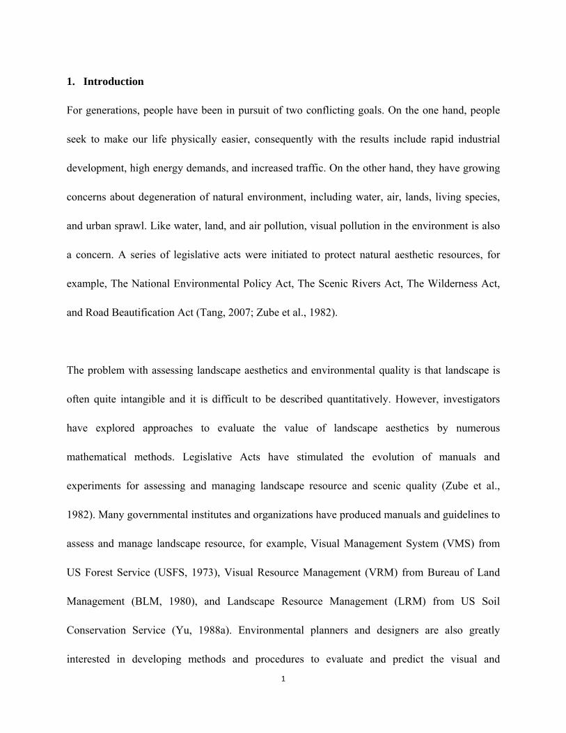
1. Introduction
For generations, people have been in pursuit of two conflicting goals. On the one hand, people
seek to make our life physically easier, consequently with the results include rapid industrial
development, high energy demands, and increased traffic. On the other hand, they have growing
concerns about degeneration of natural environment, including water, air, lands, living species,
and urban sprawl. Like water, land, and air pollution, visual pollution in the environment is also
a concern. A series of legislative acts were initiated to protect natural aesthetic resources, for
example, The National Environmental Policy Act, The Scenic Rivers Act, The Wilderness Act,
and Road Beautification Act (Tang, 2007; Zube et al., 1982).
The problem with assessing landscape aesthetics and environmental quality is that landscape is
often quite intangible and it is difficult to be described quantitatively. However, investigators
have explored approaches to evaluate the value of landscape aesthetics by numerous
mathematical methods. Legislative Acts have stimulated the evolution of manuals and
experiments for assessing and managing landscape resource and scenic quality (Zube et al.,
1982). Many governmental institutes and organizations have produced manuals and guidelines to
assess and manage landscape resource, for example, Visual Management System (VMS) from
US Forest Service (USFS, 1973), Visual Resource Management (VRM) from Bureau of Land
Management (BLM, 1980), and Landscape Resource Management (LRM) from US Soil
Conservation Service (Yu, 1988a). Environmental planners and designers are also greatly
interested in developing methods and procedures to evaluate and predict the visual and

2
ecological quality on wild and scenic rivers, scenic highways, scenic, and recreational parks,
trials, and wetlands (Burley, 1997).
Visual quality assessment is one approach for landscape professionals to analyze existing
conditions and proposed treatments. The approach often requires the use of photographic images
to assess the visual quality of the landscape. Photographs have been tested in many studies, and
investigators have demonstrated that photographs could be used as substitutes for site visits, as
there is no perceived variance between photos and real landscape (Boster, 1974; Zube, 1974).
Besides landscape planners and professional resource managers, a significant number of
individuals, including ecologists, geographers, environmental experts and psychologists are
engaging in landscape perception and assessment research, and all of them have introduced
different sets of methods and models from their disciplines (Burley, 1997; Yu, 1988b; Zube et al.,
1982). Today, four popular paradigms are universally recognized: the expert paradigm, the
psychophysical paradigm, the cognitive paradigm and the experimental paradigm (Kaplan and
Kaplan, 1989; Kaplan et al., 1989; Yu, 1988; Zube et al., 1982). Landscape perception and
assessment is often considered as a function of the interaction of humans and the landscape
(Zube et al., 1982; Zube, 1975). Besides those four paradigms, there is an increasing trend that
more and more people engage in mapping visual quality because of the growth of spatial model
and remote sensing. This project focuses on the connection concerning visual quality and
mapping.

3
2. Literature Review
Both public and experts show intense enthusiasm for landscape values, but no general
standardization of landscape values exists (Taylor et al., 1987). Many people tended to utilize
their own discipline to develop tools and methods to measure landscape aesthetics and ecological
values while ignoring existing data and methods from others (Burley, 1997; Brown, 1991; Vining
and Steven, 1986; Zube et al., 1982; Latimer et al., 1981; Malm et al., 1981;). Meanwhile there is
little agreement on how to evaluate landscape (Zube et al., 1975). After discussion and
exploration on the topic of landscape assessment for several decades, four paradigms were
identified on the basis of theoretical models and respondent participation: expert, psychophysical,
cognitive, and experiential (Kaplan and Kaplan, 1989; Kaplan et al., 1989; Zube et al., 1982; Yu,
1988b; Taylor et al., 1987; Daniel and Vining, 1983; Porteous, 1982). In the expert paradigm,
assessments are done by highly skilled experts, such as landscape planners and designers,
forestry managers and ecologists. In the psychophysical paradigm, assessing models derive from
landscape stimulus features by public respondents. In the cognitive paradigm, the core issue is to
understand meanings of landscape by terms, such as legibility, coherence, mystery, complexity,
and smoothness (Taylor et al., 1987). And the experimental paradigm emphasizes human-
landscape interaction (Yu, 1988b; Taylor et al., 1987).
2.1. The Expert Paradigm
Expert assessment of landscape quality is divided by two general traditions: fine art tradition and
ecological tradition (Taylor et al., 1987; Daniel and Vining, 1983). Laurie (1975) and Carlson

4
(1977) indicated that experts who are through their professional training are far superior judges
of landscape quality than general public. In the expert paradigm, four elements; form, line color
and texture are often described as dominance elements to assess scenic quality. In addition,
expert paradigm often takes ecological principle into account to assess landscape quality. For
example, Smardon’s experiment (1975) on inland wetland and Leopold’s experiment (1969) on
evaluating river corridor aesthetics demonstrated the importance of ecological tradition.
The expert approach has generally dominated the professional practice, including land use
planning, forest management, and correlative legislation, and has been accepted by governmental
institutes and organizations (Zube et al., 1982; Taylor et al., 1987). Manuals and guidelines to
assess and manage landscape resource, have been developed by the organizations, for example,
Visual Management System (VMS) of The U.S. Forest Service (USFS, 1973), Visual Resource
Management (VRM) of Bureau of Land Management (BLM, 1980), Visual Impact Assessment
(VIA) of Federal Highway Administration, and Landscape Resource Management (LRM) of The
U.S. Soil Conservation Service (Yu, 1988b). Management agencies explore expert ways of rating
landscapes for resource management, but their purposes vary. For instance, VMS of The U.S.
Forest Service and VRM of Bureau of Land Management target on natural landscape, and aim to
establish rational measurements by assessing the natural resources, including forest, mountain,
and water (USFS, 1973; BLM, 1980); LRM of The U.S. Soil Conservation Service targets on
country landscape; and VIA of Federal Highway Administration aims to assess influence of
5
human activities, such as construction and traffic, on landscape.
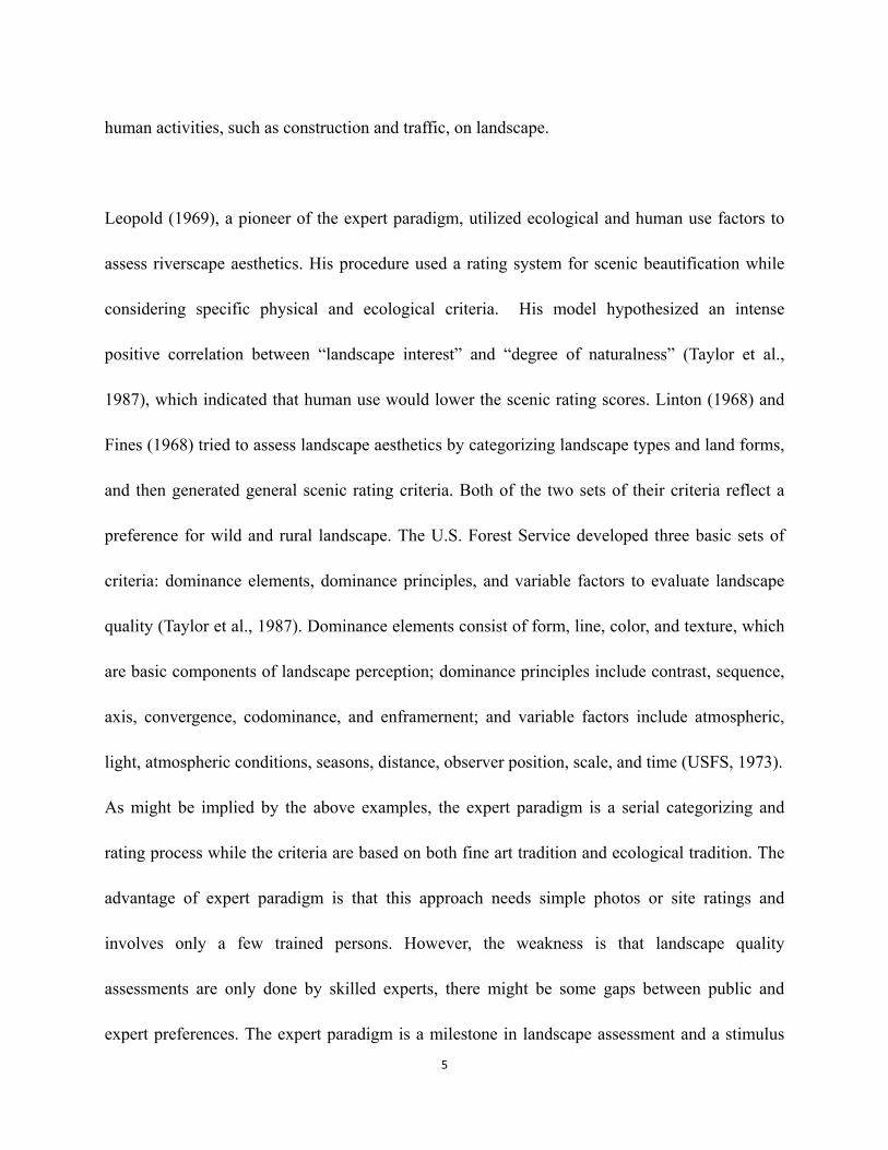
Leopold (1969), a pioneer of the expert paradigm, utilized ecological and human use factors to
assess riverscape aesthetics. His procedure used a rating system for scenic beautification while
considering specific physical and ecological criteria. His model hypothesized an intense
positive correlation between “landscape interest” and “degree of naturalness” (Taylor et al.,
1987), which indicated that human use would lower the scenic rating scores. Linton (1968) and
Fines (1968) tried to assess landscape aesthetics by categorizing landscape types and land forms,
and then generated general scenic rating criteria. Both of the two sets of their criteria reflect a
preference for wild and rural landscape. The U.S. Forest Service developed three basic sets of
criteria: dominance elements, dominance principles, and variable factors to evaluate landscape
quality (Taylor et al., 1987). Dominance elements consist of form, line, color, and texture, which
are basic components of landscape perception; dominance principles include contrast, sequence,
axis, convergence, codominance, and enframernent; and variable factors include atmospheric,
light, atmospheric conditions, seasons, distance, observer position, scale, and time (USFS, 1973).
As might be implied by the above examples, the expert paradigm is a serial categorizing and
rating process while the criteria are based on both fine art tradition and ecological tradition. The
advantage of expert paradigm is that this approach needs simple photos or site ratings and
involves only a few trained persons. However, the weakness is that landscape quality
assessments are only done by skilled experts, there might be some gaps between public and
expert preferences. The expert paradigm is a milestone in landscape assessment and a stimulus
6
for the development of alternative approaches, such as psychophysical paradigm.
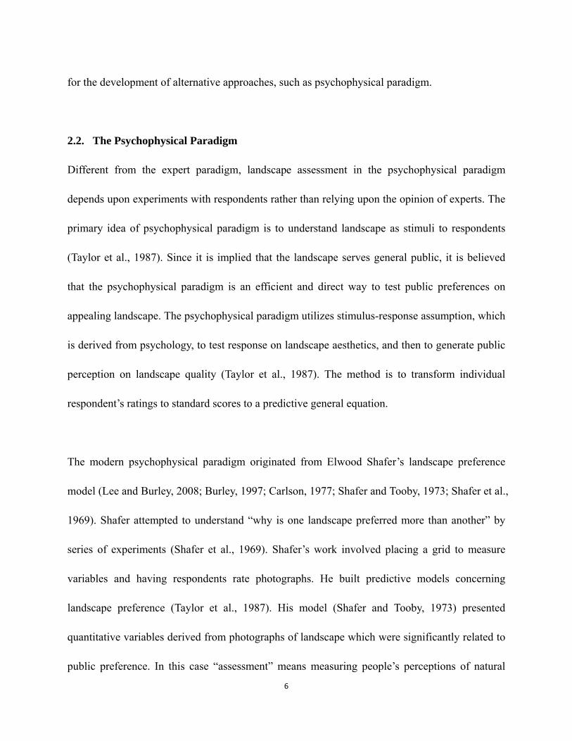
2.2. The Psychophysical Paradigm
Different from the expert paradigm, landscape assessment in the psychophysical paradigm
depends upon experiments with respondents rather than relying upon the opinion of experts. The
primary idea of psychophysical paradigm is to understand landscape as stimuli to respondents
(Taylor et al., 1987). Since it is implied that the landscape serves general public, it is believed
that the psychophysical paradigm is an efficient and direct way to test public preferences on
appealing landscape. The psychophysical paradigm utilizes stimulus-response assumption, which
is derived from psychology, to test response on landscape aesthetics, and then to generate public
perception on landscape quality (Taylor et al., 1987). The method is to transform individual
respondent’s ratings to standard scores to a predictive general equation.
The modern psychophysical paradigm originated from Elwood Shafer’s landscape preference
model (Lee and Burley, 2008; Burley, 1997; Carlson, 1977; Shafer and Tooby, 1973; Shafer et al.,
1969). Shafer attempted to understand “why is one landscape preferred more than another” by
series of experiments (Shafer et al., 1969). Shafer’s work involved placing a grid to measure
variables and having respondents rate photographs. He built predictive models concerning
landscape preference (Taylor et al., 1987). His model (Shafer and Tooby, 1973) presented
quantitative variables derived from photographs of landscape which were significantly related to
public preference. In this case “assessment” means measuring people’s perceptions of natural

7
environments. Shafer’s model could be considered as a “physical attributes” predictive model
because the variables in his model are all physical elements such as vegetation, sky, water.
However, Shafer’s model was questioned by some later studies (Bourassa, 1991; Carlson, 1977;
Weinstein, 1976), because equation based assessment on visual quality is lacking formal theory
to explain interaction between variables measured in the photos and the preferences of
respondents (Burley, 1997). For example, Carlson criticized Shafer’s method and assumption on
his research of quantifying scenic beauty; and he suggested certain alternatives to Shafer’s
assumption, which involved expert opinions and non-formalist approaches (Carlson, 1977).
Daniel and Boster (1976) developed “Scenic Beauty Estimation” (SBE) method, which involved
a standardized testing procedure. In this procedure, forest quality and quantity is measured, for
example, downed wood, tree diameter, deadwood, and low-level vegetation. They chose the term
“scenic beauty” rather than “natural beauty”, because “natural” would exclude many components,
and “beauty” could be more than visual (Daniel and Boster, 1976). SBE method asked
respondents to score landscape photographs on a 1 to 10 scale according to their own criteria,
while the photographs taken in random directions in the forest are presented in a random
sequence to avoid partial sampling procedure (Daniel and Boster, 1976). Then statistical
techniques were employed to test and analyze the reliability and validity of SBE data. SBE
showed promise as an efficient and objective way for assessing scenic beauty, and for predicting
the aesthetic consequences of alternative land uses. In addition, Daniel had explored mapping the
“scenic beauty” for road systems and road settings (Daniel and Boster, 1976; Daniel, 1977),

8
based on those SBE scores.
Besides SBE, Law of Comparative Judgment (LCJ) is another technique to utilize
psychophysical theory to evaluate landscape preference (Buhyoff et al.,1982). In LCJ experiment,
respondents are required to compare a set of photographs to generate tables of landscape
measures. Buhyoff and his colleagues set up multiple regression models to assess vista landscape,
while dependent variable is public preference and independent variables include forest area,
mountain area, and flat ground area. Although most researchers focused on studying natural
forest landscape, Buhyoff and his colleagues assessed quality of urban green space as well
(Buhyoff et al., 1984). Buhyoff and his colleagues established a mathematical model from two
aspects: like Daniel’s work, they assessed landscape elements during site visits and
established relational models based on public preferences; secondly, they directly measured
dominance components on photographs, for example, vegetation area in the photos, and then
established correlation between these components and public estheticism (Buhyoff et al., 1981).
Buhyoff’s study on urban green space showed that less large tress are more preferred as high
scenic quality than more small tress. Experiment has proved that group consensus values derived
from the Law of Comparative Judgment psychophysical scaling procedure is excellent, and
provided evidence of robustness of LCJ procedure (Buhyoff et al., 1984). However, both the
SBE and LCJ methods could be fairly time consuming in the judgments collection and data
processing, and heavily rely on high speed computers (Buhyoff et al., 1984).

9
After early pioneering experiments on psychophysical paradigms, photographs had been tested in
many studies and proved to be appropriate substitutes for site visits, as there is no perceived
variance between photos and real landscape (Boster, 1974; Zube, 1974). Nevertheless, drawings
of landscape should not be used in preference surveys (Smardon et al., 1986; Boster, 1974; Zube,
1974). Although Shafer’s model is questioned by many researchers, people from different
disciplines attempt to develop their own predictive preference equations based on Shafer’s model
to assess scenic quality (Burley, 1997; Brown, 1991; Vining and Steven, 1986; Latimer et al.,
1981; Malm et al., 1981;). Even today, the expert paradigm is still in an exploration phase, as no
expert could promise his or her method is the “canon”.
For transportation planning and design, Jon Burley developed a visual and ecological
environmental quality model that explains 67 percent of respondent preference to predict human
preference (Burley, 1997). Besides physical variables in grid measuring, he added an
“environmental quality index” in his equation. This equation has also been employed frequently
in surface mine reclamation assessment and landscape evaluation (Lu, et al., 2010; Lee and
Burley, 2008; Burley, 2006; Burley 1997). For example, Lee and Burley (2008) employed this
equation to measure two sets of photographs which were from 1980 and 2005 to compare
landscape changes after 25 years of reclamation in Plymouth, Minnesota. Burley’s model was
initially developed as a universal model across North America and illustrated its use for
transportation planning and design. According to those experimental results, his method is
applicable in many areas of natural landscape, from scenic road designs to post-mining areas. In
10
addition, Noffke and Burley (2004) used GIS based land-use data to substitute for photographs to
assess visual quality in Grand Traverse County, Michigan. This experiment suggests the
application of a remote, off-site method to measure landscape visual quality.
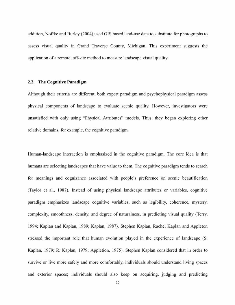
2.3. The Cognitive Paradigm
Although their criteria are different, both expert paradigm and psychophysical paradigm assess
physical components of landscape to evaluate scenic quality. However, investigators were
unsatisfied with only using “Physical Attributes” models. Thus, they began exploring other
relative domains, for example, the cognitive paradigm.
Human-landscape interaction is emphasized in the cognitive paradigm. The core idea is that
humans are selecting landscapes that have value to them. The cognitive paradigm tends to search
for meanings and cognizance associated with people’s preference on scenic beautification
(Taylor et al., 1987). Instead of using physical landscape attributes or variables, cognitive
paradigm emphasizes landscape cognitive variables, such as legibility, coherence, mystery,
complexity, smoothness, density, and degree of naturalness, in predicting visual quality (Terry,
1994; Kaplan and Kaplan, 1989; Kaplan, 1987). Stephen Kaplan, Rachel Kaplan and Appleton
stressed the important role that human evolution played in the experience of landscape (S.
Kaplan, 1979; R. Kaplan, 1979; Appletion, 1975). Stephen Kaplan considered that in order to
survive or live more safely and more comfortably, individuals should understand living spaces
and exterior spaces; individuals should also keep on acquiring, judging and predicting

11
information (S. Kaplan, 1987). Thus, in the landscape aesthetics assessment process, two terms
are identified: one is “making sense”, which focuses on suitable orientation of landscape; the
other is “involvement”, which focuses on challenge and stimulation (S. Kaplan, 1979). “Making
sense” could be immediately understood as “coherence”; and also be inferred as “legibility”
(Kaplan et al., 1989). “Involvement” immediately related to complexity (richness, intricate,
numbers of different elements, and inferential related to mystery (promise of new but related
information) (Kaplan et al., 1989). Mystery, which is a key element in cognitive model,
emphasizes an exploring process of the observers and points to the endless opportunity to see
new things, for example, the next hill or brooks behind the trees.
Several researchers in the cognitive paradigm showed great interest in cross-cultural experiments
for landscape perception. Zube and his colleagues (1973; 1976) did several cross-cultural
experiments, and found that in some of their experiments there were significant differences
between River Valley residents and college students; and in some of their experiments there were
high correlation of landscape preference, for example, between residents of Australia and college
students. By assessing photographs of lake landscapes within cross-cultural groups, Yu (1987)
summarized that the expert group has intuition in evaluating basic landscape elements associated
with ecological features, while the public group is mostly influenced by beauty in forms.
Some researchers have been involved in studies of the relationship between personality and
landscape perception. By series of experiments, Craik (1975) identified fourteen personality

12
types which might influence landscape perception. Little (1975) emphasized both “thing” and
“person” as personality dimensions.
In addition, unlike so many methodological experiments in the expert paradigm and in the
psychophysical paradigm, many cognitive researches utilized survey questions or adjective
checklist as techniques for studying (Taylor et al., 1987). For example, in Craik’s (1975) study
on San Francisco Bay Area, the respondents checked many terms describing landscape, such as
active, dark, and bushy. A landscape preference was created based on the checklist.
In the later studies, in order to avoid disadvantages of language expression of psychological tests,
Ulrich (1981) and his colleagues began to use more standard scientific test techniques, for
example, electroencephalograph (EEG) and electrocardiograph (EKG), to measure emotional
reactions objectively. Ulrich considered that the influence of natural scenes was not only as
aesthetic objects, but also directly affected human’s other physiological and psychological
reactions. His experiments proved that natural landscape scenes would significantly accelerate
patents’ recovery rate and positively influence them; but urban scenes would result in sadness for
patents (Ulrich, 1979; Ulrich, 1981).
We could see that the cognitive paradigm was gradually developed by Appleton, Kaplans, Craik,
Ulrich and other scholars to form a theoretical system, including evolution, aesthetic concept,
and emotional theory to integrally understand landscape. The problem with the approach is that
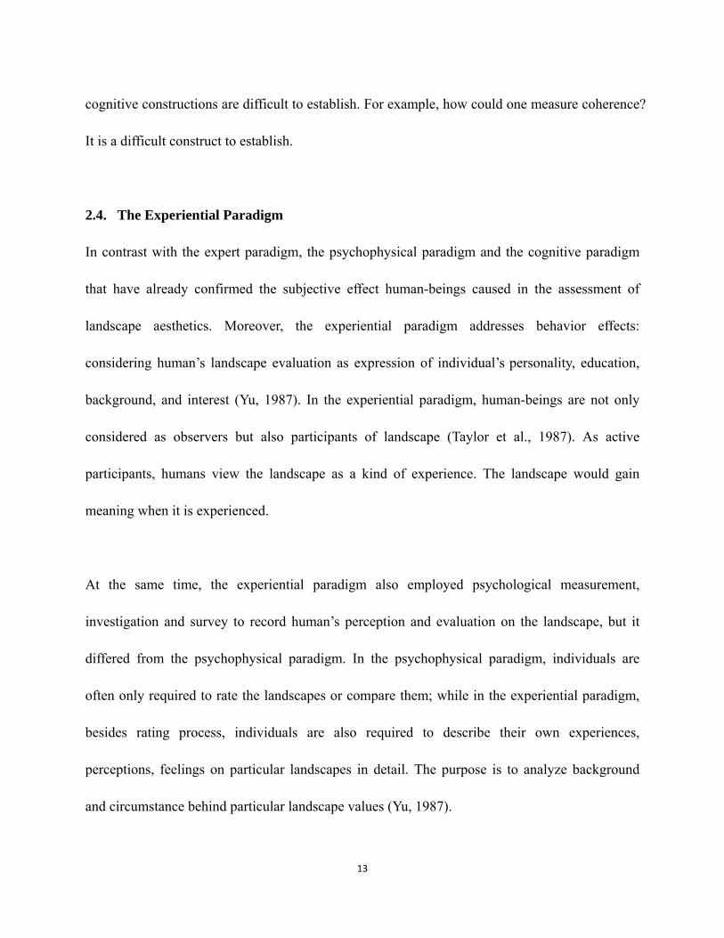
13
cognitive constructions are difficult to establish. For example, how could one measure coherence?
It is a difficult construct to establish.
2.4. The Experiential Paradigm
In contrast with the expert paradigm, the psychophysical paradigm and the cognitive paradigm
that have already confirmed the subjective effect human-beings caused in the assessment of
landscape aesthetics. Moreover, the experiential paradigm addresses behavior effects:
considering human’s landscape evaluation as expression of individual’s personality, education,
background, and interest (Yu, 1987). In the experiential paradigm, human-beings are not only
considered as observers but also participants of landscape (Taylor et al., 1987). As active
participants, humans view the landscape as a kind of experience. The landscape would gain
meaning when it is experienced.
At the same time, the experiential paradigm also employed psychological measurement,
investigation and survey to record human’s perception and evaluation on the landscape, but it
differed from the psychophysical paradigm. In the psychophysical paradigm, individuals are
often only required to rate the landscapes or compare them; while in the experiential paradigm,
besides rating process, individuals are also required to describe their own experiences,
perceptions, feelings on particular landscapes in detail. The purpose is to analyze background
and circumstance behind particular landscape values (Yu, 1987).

14
The experiential paradigm is not considered as a method to assess landscape, as it does not study
the quality of landscape; thus, the experiential paradigm rarely directly offers effective
information to landscape planning and management. As a result, the experiential paradigm is
powerless when compared with the other paradigms.
2.5. Comparison of the Four Paradigms
Some studies summarized and compared these different domains or paradigms of landscape
perception. In 1989, Kaplan et al. (1989) reported that they examined and compared four
domains: Physical Attributes, Land Cover Types, Informational Variables, and Perception-based
Variables to assess their relative benefit and deficiency in explaining environmental preference.
Their results suggested the importance of utilizing different predictor domains, rather than
relying on any single one, since their merits vary according to different study backgrounds. Some
researchers also analyzed and summarized four popular paradigms: the expert paradigm, the
psychophysical paradigm, the cognitive paradigm and the experimental paradigm to offer help in
choosing appropriate methods (Tang, 2007; Yu, 1988b; Taylor et al., 1987; Zube et al., 1982).
Each paradigm has its own strength and weakness, and might be suitable for different situations:
the expert paradigm describes landscape from the professional perspectives and could be applied
in planning, design and management decision; the psychophysical paradigm is rated mainly on
physical variables and associated with public participation; the cognitive paradigm emphasizes
understanding meanings of landscape (legibility, coherence, mystery, complexity, smoothness
and so on); and the experiential paradigm emphasizes human-landscape interaction (Taylor, et al.,

15
1987; Yu, 1988b). In short, the expert paradigm and the psychophysical paradigm focus on
landscape management practice (Terry, 2001; Yu, 1988b); while the cognitive and the
experiential seek to understand the importance of valued landscape to people. Those paradigms
have paralleled a long-standing debate in the philosophy of aesthetics (Terry, 2001; Yu, 1988b).
In general, each of the above four paradigms takes a unique approach and target on landscape
assessment. Nevertheless, if the landscape aesthetics process, as a system, is considered, it is
apparent that all different approaches are complemented rather than incompatible. For example,
the expert paradigm ignores the subjective function while the experiential paradigm emphasizes
human-beings.
2.6. Mapping Visual Quality
Because of the development of spatial modeling techniques, landscape visual quality assessment
has begun to work on a broader dimension: (1) integrating spatial models with assessment, and
(2) associating with ecological quality assessment. As Terry (2001) mentioned, technological
development such as remote sensing, three-dimensional geographic information system (GIS),
and advanced environmental modeling have improved the ability to measure ecologically
relevant landscape features, which has the potential to meet the urgent need of shifting toward
more comprehensive ecosystem management. Consequently, traditional visual quality
assessment, including expert and perception-based approaches, would be challenged by both
technological improvement and the emergence of landscape ecology.

16
Many studies have offered well-grounded evidence to support the validity of using
computer-based spatial modeling to assess landscape visual quality (Germino et al., 2001;
Dramstad et al., 2006; Bishop and Hulse, 1994; Crawford, 1994; Aamir and Gidalizon, 1990).
In early time, Brush (1979) and his colleague measured land use change in the Northwest to
illustrate the impact of urbanization on scenic quality. Aamir and Gidalizon (1990) used the
expert paradigm for quantitative evaluation of landscape visual absorption capacity (VAC), and
then used these data to output computer-printed maps in several regions with various
geographical characteristics in Israel. This method was found to be easy and effective to apply.
Bishop is a pioneer with integrating the use of GIS with the traditional method (prediction
equation) to assess landscape visual quality. The results of Bishop and Hulse’s (1994) experiment
on Oregon suggested that there existed considerable potential for use of GIS combing with a
predictor equation to map visual quality and that the mapped value at all locations would match
an assessment made by experts. Crawford (1994) used remote sensing to assess landscape visual
quality and replicated an experiment in Cook’s river, where the traditional method was used and
combined with extensive fieldwork to assess visual quality. The result of this study demonstrated
the feasibility of using remotely sensed data in the assessment of landscape visual quality and
showed the considerable savings in time and work. Dramstad (2006) tested map-derived
indicators of landscape structure in agricultural land with visual landscape preferences and found
significant positive correlations between preferences and spatial metrics. En-Mi Lim and his
colleagues (2006) tested three-dimensional computer graphic made with virtual reality modeling
language (VRML) as a stimulus for landscape assessment. The results indicated that VRML
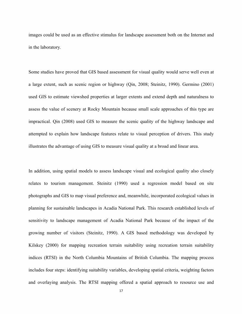
17
images could be used as an effective stimulus for landscape assessment both on the Internet and
in the laboratory.
Some studies have proved that GIS based assessment for visual quality would serve well even at
a large extent, such as scenic region or highway (Qin, 2008; Steinitz, 1990). Germino (2001)
used GIS to estimate viewshed properties at larger extents and extend depth and naturalness to
assess the value of scenery at Rocky Mountain because small scale approaches of this type are
impractical. Qin (2008) used GIS to measure the scenic quality of the highway landscape and
attempted to explain how landscape features relate to visual perception of drivers. This study
illustrates the advantage of using GIS to measure visual quality at a broad and linear area.
In addition, using spatial models to assess landscape visual and ecological quality also closely
relates to tourism management. Steinitz (1990) used a regression model based on site
photographs and GIS to map visual preference and, meanwhile, incorporated ecological values in
planning for sustainable landscapes in Acadia National Park. This research established levels of
sensitivity to landscape management of Acadia National Park because of the impact of the
growing number of visitors (Steinitz, 1990). A GIS based methodology was developed by
Kilskey (2000) for mapping recreation terrain suitability using recreation terrain suitability
indices (RTSI) in the North Columbia Mountains of British Columbia. The mapping process
includes four steps: identifying suitability variables, developing spatial criteria, weighting factors
and overlaying analysis. The RTSI mapping offered a spatial approach to resource use and

18
recreation management. Freeman and Buck (2003) developed an ecological mapping
methodology in the Dunedin city, New Zealand. In their experiment, the map is the first attempt
to record all natural land uses, and then GIS was used to map the urban habitats and store the
habitat data (Freeman and Buck, 2003). Combined mapping at a detailed level and at a broad
level was chosen as a final version to output ecological maps. Ayad (2005) integrated remote
sensing with GIS to assess visual changes in a developing coastal area of Egypt and succeeded in
detecting several changes in the attributes, and mapping the magnitude of those changes. Yasser
also suggested that the tourism resource in Egypt might be undermined if there is no
consideration of scenic value assessment in tourism management (Ayad, 2005). Mouflis and his
colleagues (2008) assessed the ecological, landscape and visual impacts of marble quarries on
the island of Thasos, Greece by mapping quarries and landscape changes. In this experiment,
remote sensing, landscape metrics and viewshed analysis were employed to monitor the
landscape dynamics (1984-2000) of marble quarries (Mouflis et al., 2008). The results
indicated that the visual impact of the quarries degraded the aesthetic impression of Thasos as a
touristic island.
Some researchers are extremely interested in assessing and mapping agricultural landscape.
Nassauer and Corry (2004) developed normative scenarios to anticipate and affect agricultural
landscape changes in Iowa. In their experiment, three distinct scenarios were proposed with
different emphases, including value of agricultural production, value of water quality and value
of biodiversity. They indicated their scenarios as a tangible goal for future landscape predictions.
19
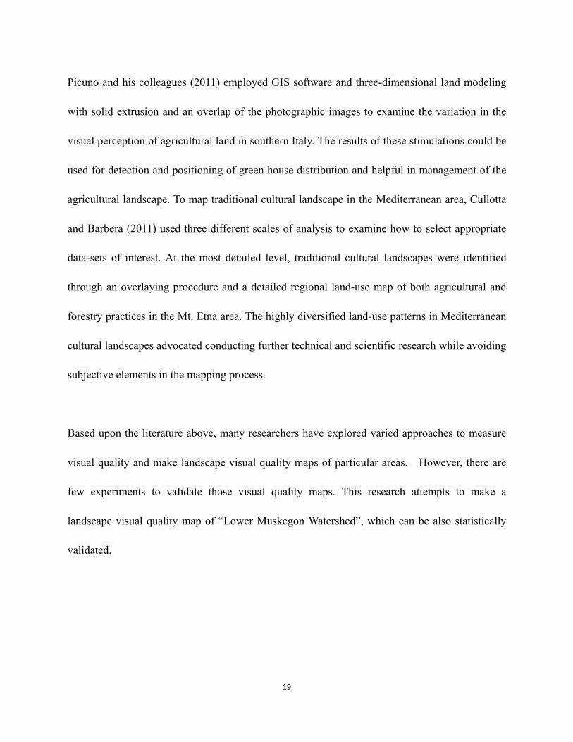
Picuno and his colleagues (2011) employed GIS software and three-dimensional land modeling
with solid extrusion and an overlap of the photographic images to examine the variation in the
visual perception of agricultural land in southern Italy. The results of these stimulations could be
used for detection and positioning of green house distribution and helpful in management of the
agricultural landscape. To map traditional cultural landscape in the Mediterranean area, Cullotta
and Barbera (2011) used three different scales of analysis to examine how to select appropriate
data-sets of interest. At the most detailed level, traditional cultural landscapes were identified
through an overlaying procedure and a detailed regional land-use map of both agricultural and
forestry practices in the Mt. Etna area. The highly diversified land-use patterns in Mediterranean
cultural landscapes advocated conducting further technical and scientific research while avoiding
subjective elements in the mapping process.
Based upon the literature above, many researchers have explored varied approaches to measure
visual quality and make landscape visual quality maps of particular areas. However, there are
few experiments to validate those visual quality maps. This research attempts to make a
landscape visual quality map of “Lower Muskegon Watershed”, which can be also statistically
validated.
20
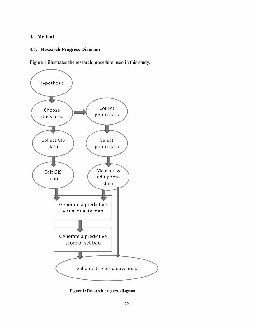
3. Method
3.1. Research Progress Diagram
Figure 1 illustrates the research procedure used in this study.
Figure 1: Research progress diagram

21
To assist planners and managers to assess landscape resources at Lower Muskegon Watershed,
this research hypothesizes: one can predict landscape aesthetic qualities of the Lower Muskegon
Watershed by producing a statistically validated landscape visual quality map, meaning that a
generated predictive map of visual quality is highly concordant with real images in the
watershed.(This research defines scores generated from Burley’s Equation 1 as real scores and
scores generated from the predictive map as predictive scores.)
3.2. Study Area
Michigan is located in the Great Lakes Region of the United States of America, with plentiful
inland lakes and river resources. Currently, a large portion of population lives in the southern part
of the Lower Peninsula but the Upper Peninsula is also important for tourism and natural
resources.
A watershed, or a drainage basin, is the area of land where surface water from rain, melting snow
and underground water drains into the same place. John Wesley Powell, scientist geographer,
defines watershed as “that area of land, a bounded hydrological system, within which all living
things are inextricably linked by their common water course and where, as humans settled,
simple logic demanded that they become part of a community” (Worster, 2009).
Muskegon River Watershed is one of the largest watersheds in the State of Michigan and spans
across nine counties: Wexford, Missaukee, Roscommon, Osceola, Clare, Mecosta, Montcalm,

22
Newaygo and Muskegon. There are several reasons that the Lower Muskegon Watershed was
chosen as the study area: (1) it is composed of several land cover types to study; (2) updated
information is readily available; and (3) it is nearby and fit within the study area of Burley’s
Equation 1 (1997). Since the late 1800s, Muskegon River Watershed drainage and riparian
vegetation were decimated by logging, constructing of dams, and forest fires (O’Neal, 1997).
During the 1900s, the expansion of urban and agricultural land use, accompanying with nutrient,
sediment, and chemical pollution have significant negative effects on the biological community
(O’Neal, 1997). Presently, people begin to consider limiting human influence on crucial habitats
and repairing the ruined environmental condition.
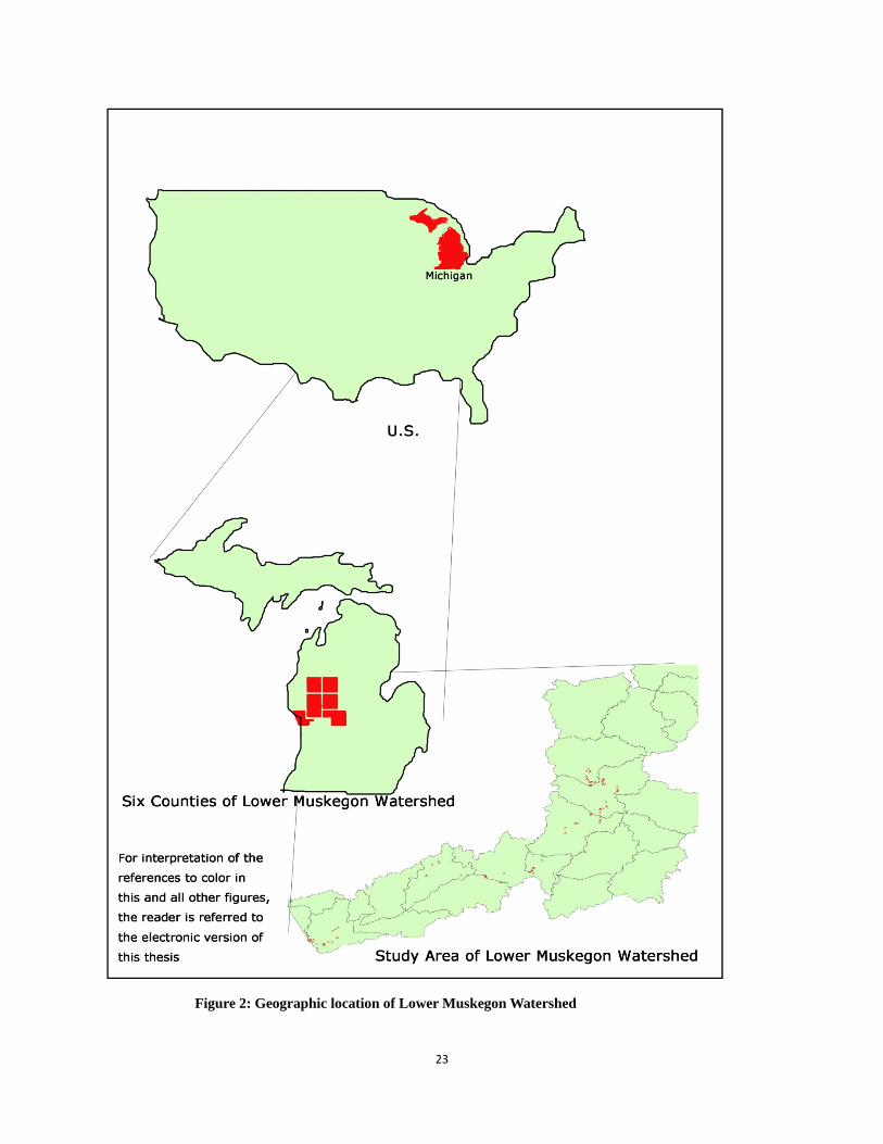
In this study, the Lower Muskegon Watershed (Figure 2) includes six counties: Muskegon
County, Lake County, Mecosta County, Montcalm County, Newaygo County, and Osceola
County. To examine our hypothesis, two crucial questions are additionally asked:
(1) What kinds of landscape are more preferred according to “Burley’s Visual Quality Equation”
in the Lower Muskegon Watershed?
(2) Are predictions (land-use map based scores) and the real photograph scores in concordance
and significant to a high confidence level?
23
Figure 2: Geographic location of Lower Muskegon Watershed

24
3.3. Collecting Data
The photos data in this study were taken by the author from site surveys on Lower Muskegon
Watershed in May and August of 2010. In May and August 2010, 131 photographs from Lower
Muskegon Watershed were recorded, and each of them was positioned and tagged on the map of
Lower Muskegon Watershed by Global Positioning System (GPS). Although the photo data were
acquired in different times of summer, there is almost no recognizable seasonal difference. The
objective and principle to collect photographs is trying to obtain different types of landscapes,
and across the study area. Typical recorded photos may contain such physical attributes as people,
wildlife, water, roads, flowers, vegetation, buildings, facilities and nonvegetated substrate across
urban savanna, farmland, forest, and watery areas. Two sets of 30 photos were chosen from the
original 131 photos to analyze. In the following study steps, set one would be used to create a
predictive landscape visual quality map while set two was employed to compare with predictions
and validate the predictive map.
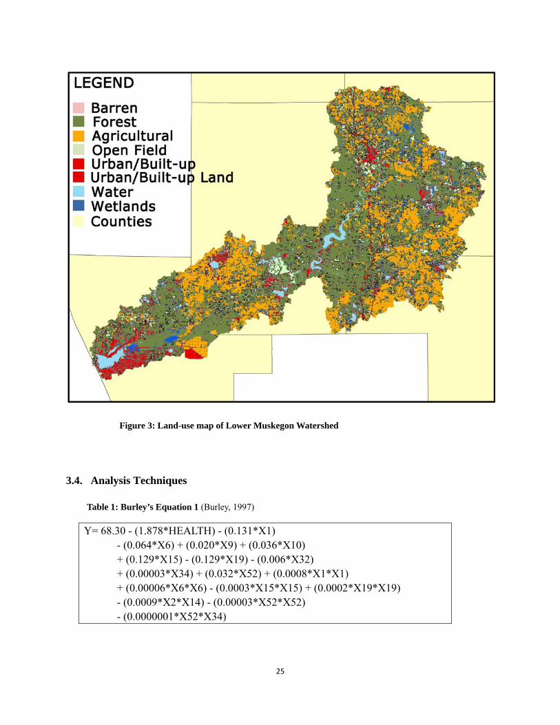
The basic GIS map data in this study were downloaded from a database of Grand Valley State
University. The project of “Sustainable Futures for the Muskegon River Watershed” from Grand
Valley State University provides all the “Updated 1998 Land Use Data” in Lower Muskegon
Watershed of six counties: Muskegon, Lake, Mecosta, Montcalm, Newaygo, and Osceola
counties. By merging all the land use data of these counties, a land-use map of Lower Muskegon
Watershed was generated (Figure 3).
25
Table 1: Burley’s Equation 1 (Burley, 1997)
3.4. Analysis Techniques
Y= 68.30 - (1.878*HEALTH) - (0.131*X1) - (0.064*X6) + (0.020*X9) + (0.036*X10) + (0.129*X15) - (0.129*X19) - (0.006*X32) + (0.00003*X34) + (0.032*X52) + (0.0008*X1*X1) + (0.00006*X6*X6) - (0.0003*X15*X15) + (0.0002*X19*X19) - (0.0009*X2*X14) - (0.00003*X52*X52) - (0.0000001*X52*X34)
Figure 3: Land-use map of Lower Muskegon Watershed

26
Table 2: Independent variables (Burley, 1997)
Variables
HEALTH= environmental quality index (Table 3.3)
X1= perimeter of immediate vegetation
X2= perimeter of intermediate non-vegetation
X3= perimeter of distant vegetation
X4= area of intermediate vegetation
X6= area of distant non-vegetation
X7= area of pavement
X8= area of building
X9= area of vehicle
X10= area of humans
X13= area of herbaceous foreground material
X14= area of wildflowers in foreground
X15= area of utilities
X16= area of boats
X17= area of dead foreground vegetation
X19= area of wildlife
X30= open landscapes = X2+X4+(2*(X3+X6))
X31= closed landscapes = X2+X4+(2*(X1+X17))
X32= openness = X30-X31
X34= mystery = X30*X1*X7/1140
X52= noosphericness = X7+X8+X9+X15+ X16
This study utilized Burley’s experimental method (Burley, 1997; Lee and Burley, 2008) to
measure photos. Each of the 30 photos from set one and set two was measured according to the
Equation 1 by Burley (1997), which is based on physical variables and environmental quality
index. The predictive model, where the equation explains 67 percent of respondent preference,
contained total area of noospheric features and total area of motorized vehicles; presence of

27
Table 3: Environmental quality index (Burley, 1997)
humans, wildlife, utility structures, and foreground flowers; total area of distant nonvegetation
landscape features such as mountains and buttes; perimeter of intermediate nonvegetation; total
area of foreground vegetation; and openness, mystery, and environmental quality index; with an
overall p-value for the equation <0.0001 and a p-value<0.05 for all regressors (Burley, 1997).
Environmental Quality Index Variable Score A. Purifies Air +1 0 -1 B. Purifies Water +1 0 -1 C. Builds Soil Resources +1 0 -1 D. Promotes Human Cultural Diversity +1 0 -1 E. Preserves Natural Resources +1 0 -1 F. Limits Use of Fossil Fuels +1 0 -1 G. Minimizes Radioactive Contamination +1 0 -1 H. Promotes Biological Diversity +1 0 -1 I. Provides Food +1 0 -1 J. Ameliorates Wind +1 0 -1 K. Prevents Soil Erosion +1 0 -1 L. Provides Shade +1 0 -1 M. Presents Pleasant Smells +1 0 -1 N. Presents Pleasant Sounds +1 0 -1 O. Does not Contribute to Global Warming +1 0 -1 P. Contributes to the World Economy +1 0 -1 Q. Accommodates Recycling +1 0 -1 R. Accommodates Multiple Use +1 0 -1 S. Accommodates Low Maintenance +1 0 -1 T. Visually Pleasing +1 0 -1
Total Score _________
In Burley’s Equation 1 (Table 1, Table 2), there is a set of regressors (regressors are the variables
from Table 2) with negative coefficients. This set of regressors positively relate to visual quality
(Burley, 1997). They include the presence of immediate vegetation and distant nonvegetation, the
28
presence of wildlife, presence of flowers and openness (X1, X6, X14, X19 and X32 from Table
2). These regressors are perceived as positive enhancement by respondents.
There is also a set of regressors with positive coefficients (Burley, 1997). This set of regressors
negatively related to visual quality (Burley, 1997). These regressors include the presence of
vehicles, humans, utility structure and overall noospheric features (X9, X10, X15 and X52 from
Table 2). This means that the more humans, vehicle, building and artificial structures in a
photograph, the worse the visual quality is.
There is a third set of regressors to be considered: neutral variables (Burley, 1997). Typical
neutral variables are sky, clouds, sun, moon, water, ice, snow and so on. They affect the presence
of both positive and negative variables. The more area these neutral variables occupy in a
photograph, the more likely the score is close to a neutral value, which is 70.
To analyze the visual quality scores of set one and set two, statistical analysis for our research is
executed in Microsoft EXCEL 2007 for Windows XP. As mentioned above, the real scores of set
two were generated according to Burley’s Equation 1. And the predicted average scores of set
two were generated from the real scores of set one. Then, the real scores of set two and the
predicted average scores of set two were ranked from 1 to 30, with the highest score receiving 1
and the lowest score receiving 30.
29
The two columns of scores were compared using Kendall’s Coefficient of Concordance (W)
(Daniel 1978), to test for similar agreement. Suppose that score i is given the rank ri, j by judge
number j, where there are in total n (30) scores and m (2) judges. Then the total rank given to
score i is
(1)
and the mean value of these total ranks is
(2)
The sum of squared deviations, S, is defined as
(3)
and then Kendall’s W is defined as (Kendall, 1939)
(4)
The test statistic W is between 0 and 1. If W is 0, there is no overall trend of agreement among
the respondents. If W is 1, the responses might be regarded as essentially random. Intermediate
values of W suggest a degree of concordance among different responses.

30
Figure 4: Locations of 131 photos at Lower Muskegon Watershed
4. Results
4.1. Mapping Visual Quality
The methodology generated a series of figures and tables. The collected 131 photographs were
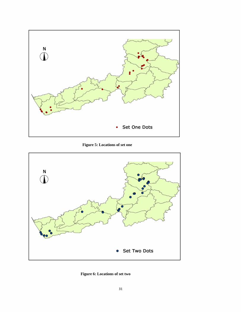
marked in the map to illustrate their locations (Figure 4). As shown in Figure 5 and Figure 6, the
locations of set one and set two were recorded in this experiment.
31
Figure 5: Locations of set one
Figure 6: Locations of set two

32
Table 4: Visual quality score of set one and set two
Visual Quality Score Set One Set Two
NO. Land Use Type Score Land Use Type Score 1 Urban Savanna 64.15325 Urban savanna 72.91732
2 Farmland 47.2868 Farmland 60.12997
3 Water 49.29968 Water 54.04903 4 Industrial 83.06227 Industrial 93.2968
5 Farmland 45.02445 Farmland 43.3638
6 Water 52.4 Water 44.4542 7 Forest 52.4952 Forest 52.3262
8 Farmland 64.63812 Farmland 51.06412
9 Water 52.89468 Water 42.1124 10 Farmland 51.5882 Farmland 51.93535
11 Downtown 78.67512 Downtown 80.84248
12 Farmland 53.00983 Farmland 48.79608 13 Forest 59.414 Forest 56.192
14 Forest 54.4982 Farmland 55.29468
15 Farmland 62.12048 Forest 48.2258 16 Water (Pier) 57.97836 Water (Urban Savanna) 72.98182
17 Farmland 42.2612 Farmland 59.01933
18 Forest (Road) 65.97347 Forest (Road) 54.71145 19 Water 49.628 Water 50.506
20 Water (Bridge) 54.47212 Water (Dam) 61.07647
21 Industrial 107.2581 Industrial 107.805 22 Downtown 80.44573 Downtown 81.84413
23 Farmland 63.35648 Farmland 41.91216
24 Urban savanna 64.24578 Urban savanna 67.92477 25 Water 48.944 Water 46.87449
26 Urban savanna 68.00453 Urban savanna 73.11433
27 Water 49.55917 Water 48.7268 28 Downtown 72.85386 Downtown 83.52013
29 Water 55.013 Water 48.1872
30 Forest 58.262 Water, Road and Forest 68.89192
Table 4 lists the visual quality scores for two sets of 30 images based on Burley’s Equation 1.
The 30 photos from set one were divided into 6 groups: downtown, industry, urban savanna,
33
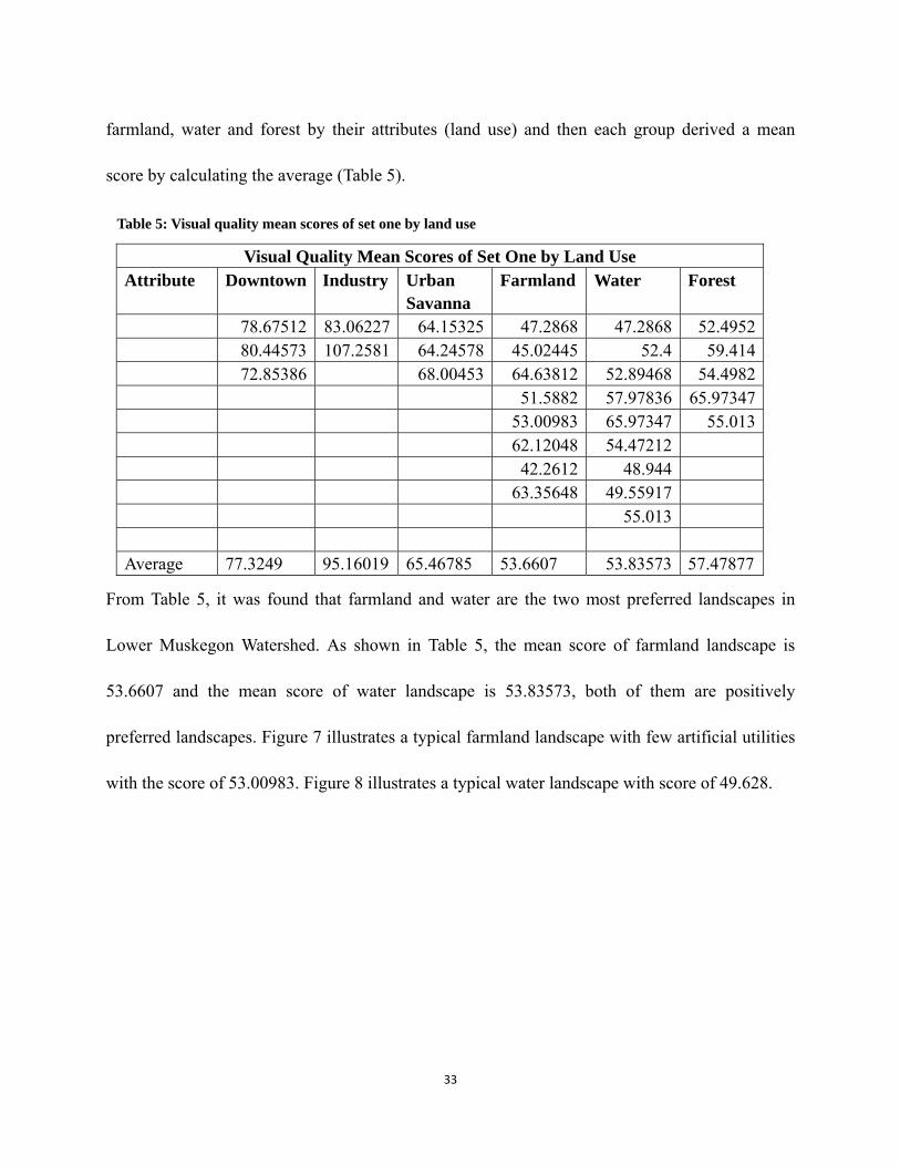
Table 5: Visual quality mean scores of set one by land use
farmland, water and forest by their attributes (land use) and then each group derived a mean
score by calculating the average (Table 5).
Visual Quality Mean Scores of Set One by Land Use Attribute Downtown Industry Urban
Savanna Farmland Water Forest
78.67512 83.06227 64.15325 47.2868 47.2868 52.4952 80.44573 107.2581 64.24578 45.02445 52.4 59.414 72.85386 68.00453 64.63812 52.89468 54.4982 51.5882 57.97836 65.97347
53.00983 65.97347 55.013 62.12048 54.47212 42.2612 48.944 63.35648 49.55917 55.013 Average 77.3249 95.16019 65.46785 53.6607 53.83573 57.47877
From Table 5, it was found that farmland and water are the two most preferred landscapes in
Lower Muskegon Watershed. As shown in Table 5, the mean score of farmland landscape is
53.6607 and the mean score of water landscape is 53.83573, both of them are positively
preferred landscapes. Figure 7 illustrates a typical farmland landscape with few artificial utilities
with the score of 53.00983. Figure 8 illustrates a typical water landscape with score of 49.628.

34
Forest landscape, with the mean score of 57.47877, and urban savanna landscape, with the mean
score of 65.46785, are positively preferred landscapes as well, but not as good as farmland and
water. Figure 9 illustrates a typical forest landscape, with score of 52.4952, while Figure 10
illustrates a typical urban savanna landscape, with score of 64.15325.
There are also negatively preferred landscapes, such as industry landscape, with the mean score
of 95.16019, and downtown landscape, with the mean score of 77.3249. Figure 11 illustrates a
typical downtown landscape, with score of 80.44573, while Figure 12 illustrates a typical
industry landscape, with score of 107.2581.
Figure 10: A typical image of urban
savanna
— Copyright © 2010, Di Lu
Figure 7: A typical image of farmland
— Copyright © 2010, Di Lu
Figure 9: A typical image of forest
— Copyright © 2010, Di Lu
Figure 8: A typical image of water
— Copyright © 2010, Di Lu

35
Figure 11: A typical image of
downtown
— Copyright © 2010, Di Lu
Figure 12: A typical image of industry
— Copyright © 2010, Di Lu
Figure 13: Predictive visual quality map

36
Table 6: Predictive scores of set two
Figure 14: A farmland image with a predictive score of 53.660695
— Copyright © 2010, Di Lu
A predictive visual quality map of Lower Muskegon Watershed (Figure 13) was generated. Table
5 shows that there are six corresponding predictive scores according to the six various land-use
types. To help validate this predictive map, the predictive scores of set two (Table 6) were
generated based on the predictive visual quality map. For example, Figure 14 is a farmland
landscape image and it acquired a predictive score of 53.660695.
NO. Score NO. Score NO. Score
1 65.46785333 11 77.32490333 21 95.160185
2 53.660695 12 53.660695 22 77.32490333
3 53.83573333 13 57.478774 23 53.660695
4 95.160185 14 53.660695 24 65.46785333
5 53.660695 15 53.660695 25 53.83573333
6 53.83573333 16 65.46785333 26 65.46785333
7 57.478774 17 53.660695 27 53.83573333
8 53.660695 18 57.478774 28 77.32490333
9 53.83573333 19 53.83573333 29 53.83573333
10 53.660695 20 53.83573333 30 58.92745

37
Table 7: Real score and predictive score of set two
4.2. Validating the Map
Set Two Image NO.
Real score Real score Ranking
Predictive Score
Predictive Score Ranking
21 107.805 1 95.160185 1.5 4 93.2968 2 95.160185 1.5 28 83.52013 3 77.32490333 4 22 81.84413 4 77.32490333 4 11 80.84248 5 77.32490333 4 26 73.11433 6 65.46785333 7.5 16 72.98182 7 65.46785333 7.5 1 72.91732 8 65.46785333 7.5 30 68.89192 9 58.92745 10 24 67.92477 10 65.46785333 7.5 20 61.07647 11 53.83573333 17.5 2 60.12997 12 53.660695 26 17 59.10933 13 53.660695 26 13 56.192 14 57.478774 12 14 55.29468 15 53.660695 26 18 54.71145 16 57.478774 12 3 54.04903 17 53.83573333 17.5 7 52.3262 18 57.478774 12 10 51.93535 19 53.660695 26 8 51.06412 20 53.660695 26 19 50.506 21 53.83573333 17.5 12 48.79608 22 53.660695 26 27 48.7268 23 53.83573333 17.5 15 48.2258 24 53.660695 26 29 48.1872 25 53.83573333 17.5 25 46.87449 26 53.83573333 17.5 6 44.4542 27 53.83573333 17.5 5 43.3638 28 53.660695 26 9 42.1124 29 53.83573333 17.5 23 41.91216 30 53.660695 26
In Table 7 the real scores ranked from high to low, with 107.805 assigned as the highest score
and 41.91216 assigned as the lowest score; while the predictive scores ranked according to
38
corresponding original image numbers and their attributes. Each column of scores has an
associated ranking. In Kendall’s Coefficient of Concordance, a W value of 0.851112347 was
generated. A corresponding Chi-Square table was consulted to determine if the derived value for
Chi-Square was significant (p≤0.05) at twenty-nine degrees of freedom (Daniel, 1978). Since the
derived value of 49.36451613 is greater than the table value of 42.55697, the null hypothesis was
rejected and the hypothesis that the two sets of numbers are in concordance (p≤0.05) was
accepted. It was determined, through statistical analysis, that the relationship of predictions
(land-use map based scores) and the real photographs are in concordance and significant to a
high (95%) confidence level.

39
Figure 15: Graphs of 95% confidence tails for visual preference scores: the
95% confidence scores for Figure 5.2 (63.35648) and Figure 5.3 (80.44573)
5. Discussion
The findings on visual quality assessment at Lower Muskegon Watershed are consistent with
many previous studies (Lee and Burley, 2008; Burley, 1997; Yu, 1988; Kaplan, S., 1979; Shafer,
et al., 1969): in general, natural landscapes are more preferred than highly disturbed human
landscape.

40
Figure 16: A typical downtown image with the score of 80.44573
— Copyright © 2010, Di Lu
It is possible to compare various photographs by constructing a plot of the predicted mean score
for a statistical equation and then calculating the 95% confidence tables for the mean scores
(Burley, 1997). A graph was constructed to illustrate the confidence plots (Figure 15).
Comparisons between scores from various images were made horizontally by determining
whether there is an overlap between the two tails (Burley, 1997). The confidence tails for Figure
16 and Figure 17 do not overlap in Figure 15, and thus it is possible to conclude the two images
are significantly different.
As shown in Figure 16 and Figure 17, a farmland image (63.35648) has a better score in visual
quality assessment than a downtown image (80.44573) because of less artificial structures and
more natural elements. It also indicated humans’ preference for rural and natural landscape.

41
Figure 17: A typical farmland image with the score of 63.35648
— Copyright © 2010, Di Lu
Figure 18: A random farmland image with the predictive score of
53.660695 — Copyright © 2010, Di Lu
The predictive visual quality map suggested that each random landscape image that is taken from
Lower Muskegon Watershed, and is qualified for each of the six land use types, would easily
have a predictive score of visual quality. For example, Figure 18 illustrates a random farmland
image with a predictive score of 53.660695. Even if a random photograph consists of mixed land
use types of landscape, there would be a predictive averaged score for it. Figure 19 is another
example of a mixed land use image.

42
Figure 19: A random mixed image of urban savanna, water and
forest with the predictive average score of 58.92745
— Copyright © 2010, Di Lu
In this research, many more photo samples could be taken to create a landscape visual quality
map; but for this research I was more interested in determining if only a few (30) number of
images would generate significant results. The reason was that by using fewer photos, this
research could examine the methodology to test for significant concordance (95%) under less
than ideal conditions and save money and time. Thus, only 30 pairs of images were chosen but
with high variation (from rural to urban landscape) to test the ability of the methodology in
assessing landscape visual quality. The results suggest that this methodology works.
Additionally, many previous investigations demonstrated the validity of using surveys, such as
respondent groups in landscape evaluation experiments (Chen et al., 2009; Burley, 1997; Yu,
1988; Buhyoff et al., 1984; Daniel and Boster, 1976; Boster, 1974; Zube, 1974). Nevertheless, in
this experiment, no respondent group was employed to evaluate landscape images, although the
equation utilized (Burley’s Equation 1) was generated from a respondent group study (Burley,

43
1997). It might be faster and more objective if this experiment does not involve people-based
surveys. Another issue in this experiment is the accuracy and reliability of these studying
photographs. Possible incomplete and bias photographs might influence the structure of this
study. A systematic way of taking photographs was used in this study: including assessing near
view visual quality, median view distance and horizontal viewshed (Chen et al., 2009; Clay and
Marsh, 2001). Thus, as presented in this study, a defined method for shooting pictures would
make this research highly reliable and reproducible.
In the context of landscape planning and design, landscape visual quality assessments are
sometimes considered not important because they lack substantial evidences or due to their
subjectivity (Ewald, 2001). The GIS based land use-map might be used in this context to
facilitate a reinforcement of visual quality assessment dealing with aesthetic depreciation. The
result of this experiment suggests that a GIS based land-use map could serve in visual quality
assessment as well as in the professional practices of landscape planning. Land-use maps could
be used to measure landscape quality instead of real images. With the help of GIS based land-use
maps, initial site surveys might be reduced. Designers and planners are able to use predictive
equations and GIS data during the early design phase. However, predicting site-assessed visual
quality does not mean that replacing public and expert assessment is advocated.
In an environmental impact assessment, visual quality assessment is an important factor as well.
Many of the environment impact properties could not be measured easily because these
44
indicators are very subjective. With the help of GIS based land-use maps to predict potential
visual impact, it might supply a quantitative method for environmental impact assessment. For
example, as it is known that the predictive visual quality score of farmland is significantly better
than the predictive score of industry in Lower Muskegon Watershed. If the developers initiate to
build a factory at a farmland area of Lower Muskegon Watershed, it is obvious that the report of
visual impact assessment would be negative according to the predictive model presented in this
study.
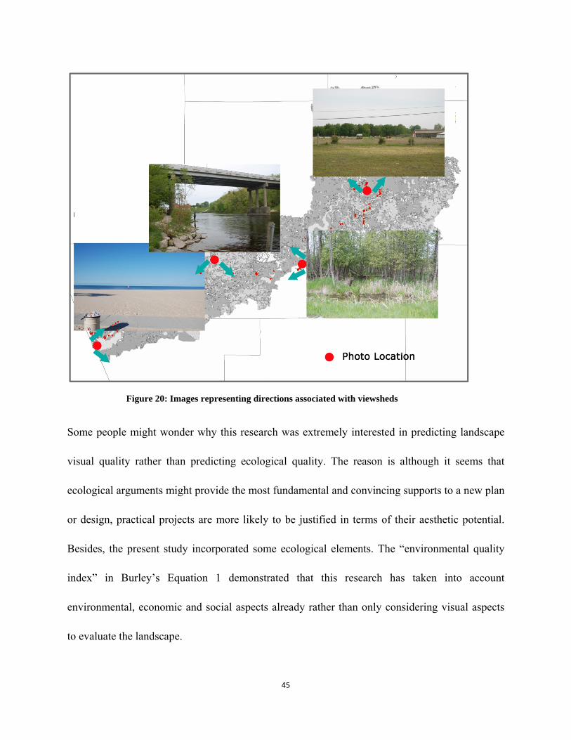
The results of the experiment could also help managing viewsheds. A viewshed is an area of land,
water, or other environmental element that is visible to the human eye from a fixed vantage point.
In this paper, the area covered by each recorded photograph is defined as a viewshed. An
example of four images and the direction of the viewsheds is shown in Figure 20. As well as
illustrated in this example, all the photo data collocated and located in this paper could be used
for later viewsheds management research.
45
Figure 20: Images representing directions associated with viewsheds
Some people might wonder why this research was extremely interested in predicting landscape
visual quality rather than predicting ecological quality. The reason is although it seems that
ecological arguments might provide the most fundamental and convincing supports to a new plan
or design, practical projects are more likely to be justified in terms of their aesthetic potential.
Besides, the present study incorporated some ecological elements. The “environmental quality
index” in Burley’s Equation 1 demonstrated that this research has taken into account
environmental, economic and social aspects already rather than only considering visual aspects
to evaluate the landscape.

46
6. Limitation
Although the potential for GIS-based land-use map seems endless, the limitations of land-use
map in visual quality studies are obvious as well. In this research, the land-use map which has
been chosen with only six categories: farmland, forest, water, urban savanna, industry, and
downtown. It is not sure, if a land-use map has more than these six categories or a photograph is
with a special landscape type, if it would still be an effective way to predict landscape visual
quality. For example, a typical photo taken from the Grand Canyon (Figure 21) might not work
in this experiment because that special landscape type is not included in the land-use map of
Lower Muskegon Watershed, although Burley’s Equation 1 was generated all across U.S.
(Burley, 1997). Sometimes, land-use map based scores are confused in adjacent areas, for
example, in an image containing a mix of farmland, water and forest. It is not always accurate or
reliable to use the average score as the predictive score of mixed landscape. In addition, land-use
map based scores could easily cover a wide area of research sites; however they could not be
assigned to a specific view or place. In those situations, site visits would become crucial:
photographs corresponding to land-use maps should be recorded and measured to solve those
problems.

47
Figure 21: A typical photo of the Grand Canyon
— Copyright © 2011, Di Lu
In addition, there are also some limitations in the current equation, especially with
“environmental quality index”. As “environmental quality index” is a subjective test, human
sense would significantly influence the results. It is entirely possible that various respondents
might perceive visual quality differently. For example, if a person extremely likes an industrial
property, his perception on this property would be more positive than others. Meanwhile better
and more independent variables are expected for this equation.
While this research has some limitations, the methodology presented in this article might provide
some inspirations in the landscape assessment and management in the Lower Muskegon
48
Watershed. For example, landscape planners could use the land-use map created in this study to
predict landscape visual quality or landscape change in the Lower Muskegon Watershed.
However, the methodology does not necessarily support the use of the predictive equation in
other areas. Some studies have shown that there is a relationship between landscape aesthetics
and visual impact of objects relevant to their scale (Shang and Bishop, 2000). Further
experiments could be carried out on a broader scale, such as the whole area of Michigan or North
America. This paper also raises some questions regarding future research:
(1) How would the results be affected if more updated GIS data is used in the research? Current
work is under the “Updated 1998 Land Use Data”, which is somewhat dated.
(2) Seasonal and annual changes in the landscape should be considered. This research only
assessed photographs in the summer while the studying area is full of leafed vegetation. How
would the results be affected if studying images were recorded during the winter?
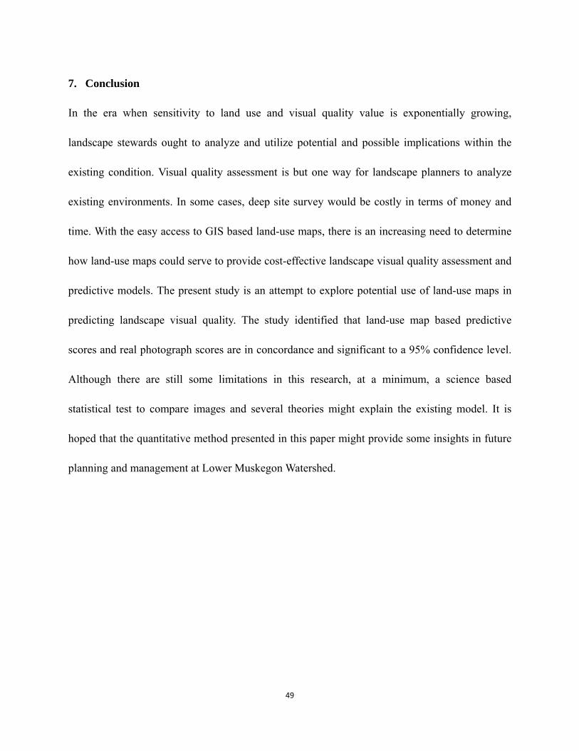
49
7. Conclusion
In the era when sensitivity to land use and visual quality value is exponentially growing,
landscape stewards ought to analyze and utilize potential and possible implications within the
existing condition. Visual quality assessment is but one way for landscape planners to analyze
existing environments. In some cases, deep site survey would be costly in terms of money and
time. With the easy access to GIS based land-use maps, there is an increasing need to determine
how land-use maps could serve to provide cost-effective landscape visual quality assessment and
predictive models. The present study is an attempt to explore potential use of land-use maps in
predicting landscape visual quality. The study identified that land-use map based predictive
scores and real photograph scores are in concordance and significant to a 95% confidence level.
Although there are still some limitations in this research, at a minimum, a science based
statistical test to compare images and several theories might explain the existing model. It is
hoped that the quantitative method presented in this paper might provide some insights in future
planning and management at Lower Muskegon Watershed.

50
Appendix

51
Figure 22: Set one NO.1
— Copyright © 2010, Di Lu
Figure 23: Set one NO.2
— Copyright © 2010, Di Lu
Figure 24: Set one NO.3
— Copyright © 2010, Di Lu Figure 25: Set one NO.4
— Copyright © 2010, Di Lu
Figure 28: Set one NO.7
— Copyright © 2010, Di Lu Figure 29: Set one NO.8
— Copyright © 2010, Di Lu
Figure 26: Set one NO.5
— Copyright © 2010, Di Lu Figure 27: Set one NO.6
— Copyright © 2010, Di Lu

52
Figure 30: Set one NO.9
— Copyright © 2010, Di Lu
Figure 31: Set one NO.10
— Copyright © 2010, Di Lu
Figure 32: Set one NO.11
— Copyright © 2010, Di Lu
Figure 33: Set one NO.12
— Copyright © 2010, Di Lu
Figure 34: Set one NO.13
— Copyright © 2010, Di Lu
Figure 35: Set one NO.14
— Copyright © 2010, Di Lu
Figure 35: Set one NO.15
Figure 37: Set one NO.16
— Copyright © 2010, Di Lu
Figure 36: Set one NO.15
— Copyright © 2010, Di Lu
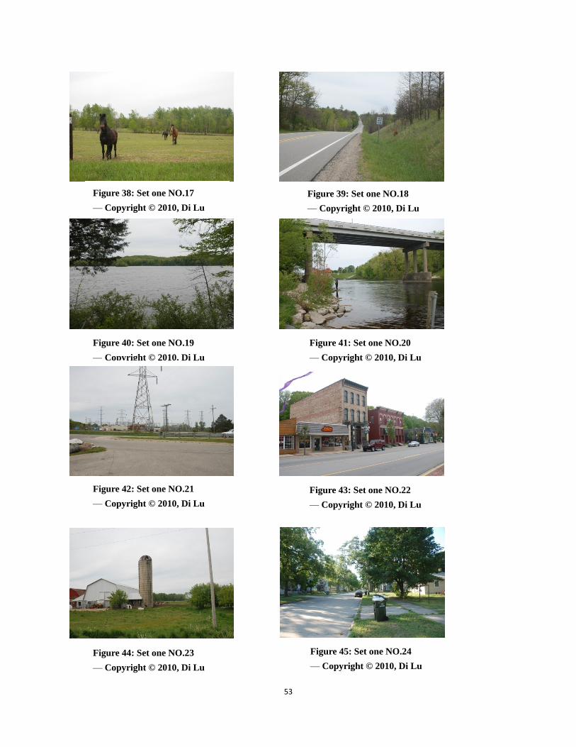
53
Figure 44: Set one NO.23
— Copyright © 2010, Di Lu
Figure 45: Set one NO.24
— Copyright © 2010, Di Lu
Figure 42: Set one NO.21
— Copyright © 2010, Di Lu
Figure 43: Set one NO.22
— Copyright © 2010, Di Lu
Figure 38: Set one NO.17
— Copyright © 2010, Di Lu
Figure 41: Set one NO.20
— Copyright © 2010, Di Lu
Figure 39: Set one NO.18
— Copyright © 2010, Di Lu
Figure 40: Set one NO.19
— Copyright © 2010, Di Lu

54
Figure 52: Set two NO.1
— Copyright © 2010, Di Lu
Figure 53: Set two NO.2
— Copyright © 2010, Di Lu
Figure 50: Set one NO.29
— Copyright © 2010, Di Lu
Figure 51: Set one NO.30
— Copyright © 2010, Di Lu
Figure 49: Set one NO.28
— Copyright © 2010, Di Lu
Figure 48: Set one NO.27
— Copyright © 2010, Di Lu
Figure 46: Set one NO.25
— Copyright © 2010, Di Lu
Figure 47: Set one NO.26
— Copyright © 2010, Di Lu

55
Figure 60: Set two NO.9
— Copyright © 2010, Di Lu
Figure 61: Set two NO.10
— Copyright © 2010, Di Lu
Figure 58: Set two NO.7
— Copyright © 2010, Di Lu
Figure 59: Set two NO.8
— Copyright © 2010, Di Lu
Figure 56: Set two NO.5
— Copyright © 2010, Di Lu
Figure 57: Set two NO.6
— Copyright © 2010, Di Lu
Figure 55: Set two NO.4
— Copyright © 2010, Di Lu
Figure 54: Set two NO.3
— Copyright © 2010, Di Lu
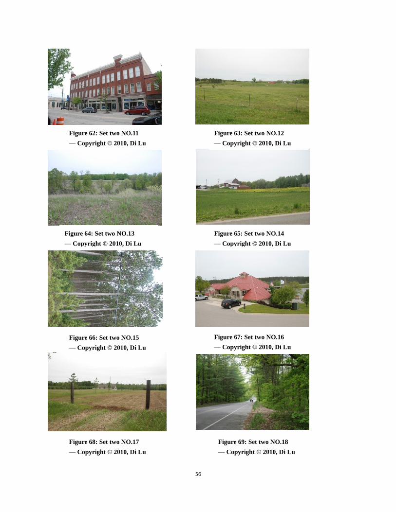
56
Figure 68: Set two NO.17
— Copyright © 2010, Di Lu
Figure 69: Set two NO.18
— Copyright © 2010, Di Lu
Figure 67: Set two NO.16
— Copyright © 2010, Di Lu
Figure 66: Set two NO.15
— Copyright © 2010, Di Lu
Figure 65: Set two NO.14
— Copyright © 2010, Di Lu
Figure 64: Set two NO.13
— Copyright © 2010, Di Lu
Figure 62: Set two NO.11
— Copyright © 2010, Di Lu
Figure 63: Set two NO.12
— Copyright © 2010, Di Lu
57
Figure 77: Set two NO.26
— Copyright © 2010, Di Lu
Figure 76: Set two NO.25
— Copyright © 2010, Di Lu
Figure 75: Set two NO.24
— Copyright © 2010, Di Lu Figure 74: Set two NO.23
— Copyright © 2010, Di Lu
Figure 73: Set two NO.22
— Copyright © 2010, Di Lu Figure 72: Set two NO.21
— Copyright © 2010, Di Lu
Figure 71: Set two NO.20
— Copyright © 2010, Di Lu Figure 70: Set two NO.19
— Copyright © 2010, Di Lu

58
Figure 81: Set two NO.30
— Copyright © 2010, Di Lu
Figure 80: Set two NO.29
— Copyright © 2010, Di Lu
Figure 78: Set two NO.27
— Copyright © 2010, Di Lu
Figure 79: Set two NO.28
— Copyright © 2010, Di Lu

59
Bibliography

60
Bibliography
Amir, S., Gidalizon, E., 1990. Expert-based method for the evaluation of visual absorption capacity of the landscape. Journal of Environmental Management. 30, 251–263. Aoki, Y., 1999. Review article: Trends in the study of the psychological evaluation of landscape. Landscape Research. 24(1), 85–94. Appleton, J., 1975. The experience of landscape. New York: Wiley. Ayad, Y. M., 2005. Remote sensing and GIS in modeling visual landscape change: a case study of the northwestern arid coast of Egypt. Landscape and Urban Planning. 73, 307–325. Bishop, I.D., Hulse, D.W., 1994. Prediction of scenic beauty using mapped data and geographic information systems. Landscape and Urban Planning. 30, 59–70. Boster, R.S., Daniel, T.C., 1974. Measuring public responses to vegetative management. Proc., 16th Annual Arizona Watershed Symposium. Arizona Water Commission. Bourassa, S.C., 1991. The aesthetic of landscape. Belhaven Press. Brown, T.C., Daniel, T.C., 1991. Landscape aesthetics of riparian environments: relationship of flow quantity to scenic quality along a wild and scenic river. Water Resource Research. 1787–1795. Brush, O. R., Palmer, J.F., 1979. Measuring the impact of urbanization on scenic quality: land use change in the Northeast. Presented at the National Conference on Applied Techniques for Analysis and Management of the Visual Resource, Incline Village, Nevada. Buhyoff, G.J., Arndt, L.K., Propst, D.B., 1981. Interval scaling of landscape preference by direct- and indirect-measurement methods. Landscape Planning. 8, 257–267. Buhyoff, G.J., Wellman, J. D., Daniel, T. C., 1982. Predicting scenic quality for Mountain Pine Beetle and Western Spruce Budworm damaged forest vistas. Forest Science. 28, 827-838. Buhyoff, G.J., Wellman, J. D., Harvey, H., and Fraser, R. A., 1978. Landscape architects’ interpretations of people’s landscape preferences. Journal of Environmental Management. 6, 255–262. Bureau of Landscape Management (BLM). 1980. Visual Resource Management Program.

61
Department of Interior. Burley, J.B., 1997. Visual and ecological environmental quality model for transportation planning and design. Transportation Research Record. 1549, 54–60. Carlson, A. A., 1977. On the possibility of quantifying scenic beauty. Landscape Planning. 4, 131–172. Chen, B., Ochieng, A. A., Bao, Z., 2009. Assessment of aesthetic quality and multiple functions of urban green space from the users’ perspective: The case of Hangzhou Flower Garden, China. Landscape and Urban Planning. 93, 76–82. Clay, G.R., Marsh, S.E., 2001. Monitoring forest transitions using scanned ground photographs as a primary data source. Photogramm. Eng. Remote Sens. 67 (3), 319–330. Craik, K.H., 1975. Individual variations in landscape description. In Landscape Assessment: Values, Perceptions, and Resources, ed. E. H. Zube. R. O. Brush, and J. g. Fabos. 130–150. Stroundsburg. Crawford, D., 1994. Using remotely sensed data in landscape visual quality assessment. Landscape and Urban Planning. 30, 7l–81. Cullotta, S., Barbera, G., 2011. Mapping traditional cultural landscapes in the Mediterranean area using a combined multidisciplinary approach: Method and application to Mount Etna (Sicily; Italy). Landscape and Urban Planning. 100, 98–108. Daniel, T. C., Anderson, L. M., Schroeder, H. W., Wheeler, L., 1977. Mapping the scenic beauty of forest landscape. Leisure Science. 1, 35–52. Daniel, T. C., Boster, R. S., 1976. Measuring landscape esthetics: the scenic beauty estimation method. USDA Forest Service, Research Paper RM- 167. Fort Collins, Colo. Daniel, T. C., Vining, J., 1983. Methodological issues in the assessment of visual landscape quality. In Behavior and the Natural Environmenta. Ed. I. Altman and J.WOHLWILL, 39–84. New York. Daniel, W.W., 1978. Applied nonparametric statistics. Houghton Mifflin Company, 326–335. Donald, W., 2009. A river running west: reflections on John Wesley Powell. Journal of Cultural. Geography. 26: 2, 113–126.

62
Dramstad, W.E., Tveit, M. S., Fjellstad, W.J., Fry, G.L.A., 2006. Relationships between visual landscape preferences and map-based indicators of landscape structure. Landscape and Urban Planning. 78, 465–474. Ewald, K.C., 2001. The neglect of aesthetics in landscape planning in Switzerland. Landscape and Urban Planning. 54, 255-266. Fines, K.D., 1968. Landscape evaluation: A research project in East Sussex. Regional Studies. 2, 41–55. Freeman, C., Buck, O., 2003. Development of an ecological mapping methodology for urban areas in New Zealand. Landscape and Urban Planning. 63, 161–173. Germino, M. J., Reiners, W. A., Blasko, B.J., McLeod, D., Bastian, C.T., 2001. Estimating visual properties of Rocky Mountain landscapes using GIS. Landscape and Urban Planning. 53, 71–83. Gonzalo, de la Fuente de Val., Jose, A. Atauri., Jose, V. de Lucio., 2006. Relationship between landscape visual attributes and spatial pattern indices: A test study in Mediterranean-climate landscapes. Landscape and Urban Planning. 77, 393–407. Hadrian, D.R., Bishop, I.D., Mitcheltree, R., 1988. Automated mapping of visual impacts in utility corridors. Landscape and urban Planning. 16, 261–282. Hull, R. B., Buhyoff, G.J., 1984. Individual and group reliability of landscape assessments. Landscape Planning. 11, 67–71. Kaplan, R., 1979. Visual resources and the public: An empirical approach. In Our National Landscape, ed. G. H. Elsner and R.C. Smardon, 209–216. USDA Forest Serivce, General Technical Report PSW-35. Berkeley. Kaplan, R., Kaplan, S., 1989. The experience of nature. Cambridge University Press. Kaplan, R., Kaplan, S., Brown, T.J., 1989. Environmental preference: a comparison of four domains of predictors. Environment and Behavior. 21, 509–503. Kaplan, S., 1979. Perception and landscape: Conceptions and misconception. In Our National Landscape, ed. G. H. Elsner and R.C. Smardon, 241-248. USDA Forest Serivce, General Technical Report PSW-35. Berkeley. Kaplan, S., 1987. Aesthetics, Affect, and Cognition: Environmental preference from an evolutionary perspective. Environment and Behavior. 19, 3–32. Landscape Urban Planning. 54,
63
255–266. Kaplan. S., 1987. Aesthetics, affect, and cognition: environmental preference from an evolutionary perspective. Environment and Behavior. 19, 3–32. Kendall, M.G., 1939. “The problem of m rankings”. The annals of mathematical statistics. 10(3), 275-287. Kliskey, A.D., 2000. Recreation terrain suitability mapping: a spatially explicit methodology for determining recreation potential for resource use assessment. Landscape and Urban Planning. 52, 33–43. Latimaer, D.A., Hogo, H., Daniel, T.C., 1981. The effects of atmospheric optical condition on perceived scenic quality. Atmospheric Environment. 15, 1865–1874. Laurie, I. C., 1975. Aesthetic factors in visual evaluation. In Landscape assessment: Values, Perceptions and Resources. Ed. E. H. Zube, R. O. Brush, and J. G. Fabos. 102–118. Lee, E.J., Burley, J.B., 2008. Assessing visual quality change 25 years after post-mining housing development in Plymouth, Minnesota. 2008 National Meeting of the American Society of Mining and Reclamation, Richmond, VA. Leopold, L.B., 1969. Quantitative comparisons of some aesthetic factors among river. U.S. Department of Interior. U.S. Geological Survey Circular 620. Washington, D.C. Lim, E., Honjo, T., Umeki, K., 2006. The validity of VRML images as a stimulus for landscape assessment. Landscape and Urban Planning. 77, 80–93. Little, B. R., 1975. Specialization and varieties of environmental experience: empirical studies within the personality paradigm. In Experiencing the Environment, ed. S. Wapner, S. B. Cohen, and B. Kaplan, 81–116. New York: Plenum. Litton, D., 1968. The assessment of scenery as a natural resource. Scottish Geographical Magazines. 84, 219–293. Litton, R.B., 1968. Forest landscape description and inventories. USDA Forest Service, Research Paper. Lu, D., Xia, Q., Lu, J., Assessing visual quality change twelve years after post-mining planting on Mufu Mountain, Nanjing, Harmony and prosperity, Traditional Inheritance and Sustainable Development. 47th IFLA Congress & CHSLA Annual Meeting, Suzhou, China, 2010
64
Malm, W., Kelley, K., Molenar, J., Daniel, T., Human perception of visual air quality. Atmospheric Environment. 15, 1875–1890. Mouflis, G.D., Gitas, I. Z., Iliadou, S., Mitri, G. H., 2008. Assessment of the visual impact of marble quarry expansion (1984-2000) on the landscape of Thasos island, NE Greece. Landscape and Urban Planning. 86, 92–102. Nassauer, J. I., Corry, R. C., 2004. Using normative scenarios in landscape ecology. Landscape Ecology. 19, 343–356. Noffke, M., Burley, J.B., 2004. Predicting visual quality with GIS based land-use data: an old Mission Peninsula, Michigan case study. P. 1-12. 83rd Annual Meeting. Transportation Research Board of National Academics, 04(2297). O’Neal, R. P.,1997, Muskegon river watershed assessment. Picuno, P., Tortora, A., Capobianco, R. L., 2011. Analysis of plasticulture landscapes in southern Italy through remote sensing and solid modeling techniques. Landscape and Urban Planning. 2011, 45–56. Porteous, D., 1982. Approaches to environmental aesthetics. Journal of Environmental Psychology. 2, 53–66. Qin, X., Meitner, M., Zhang, X.,Chamberlain, B.B., 2008. Developing scenic highway design guidelines using GIS and landscape visualizations. In Proceedings. 2008 ESRI Education Users conference, August 2008. San Diego. California. 10 pp (CD), ESRI Press. Shafer Jr., E., Hamilton Jr., J.F., Schmidt, E.A., 1969. Natural landscape preference: a predictive model. Journal of Leisure Research. 1, 1–19. Shafer Jr., E., Tooby, M., 1973. Landscape preference: an international replication. Journal of Leisure Research. 5, 60–65. Shang, H., Bishop, I.D., 2000. Visual thresholds for detection, recognition and visual impact in landscape settings. J. Environ. Psychol. 20, 125–140. Smardom, R., Palmer, J., Felleman, J., 1986.Foundations for visual project analysis. A Wiley-Interscience Publication. Smardon, R. C., 1975. Assessing visual-cultural values of inland wetlands in Massachusetts. In Landscape assessment: Values, Perceptions and Resources. Ed. E. H. Zube, R. O. Brush, and J. G.

65
Fabos. 289–318. Steinitz, C., 1986. World conference on education for landscape planning. Landscape and Urban Planning. 13, 329-332. Steinitz, C., 1990. Toward a sustainable landscape with high visual preference and high ecological integrity: the loop road in Acadia National Park, U.S.A. Landscape and Urban Planning. 19, 213–250. Steinitz, C., 2001. Visual evaluation models: some complicating questions regarding memorable scenes. Landscape and Urban Planning. 54, 283–287. Tang, X., 2007. Landscape visual environment assessment (LVEA): concept, origin and development. Journal of Shanghai Jiaotong University. In Chinese. Taylor, J. G., Zube, E. H., Sell., J. L., 1987. Landscape assessment and perception research methods. p. 361-393. Methods in Environmental and Behavioral Research. Van Nostrand Reinhold Company. Tyrvainen, L., 2006. Visualization and landscape laboratories in planning, design and management of urban woodlands. Forest Policy and Economics. 8, 811–823. Ulrich, R. S., 1979. Visual landscape and psychological well-being. Landscape Research. 4, 17–23. Ulrich, R. S., 1981. Natural versus urban scenes: some psycho physiological effects. Environment and Behavior. 13, 523–556. United State Forest Service. 1973. National forest landscape management. U.S. Department of Agriculture, Agriculture Handbook no. 434. U.S. Government Printing Office. Vining, J., Stevens, J.J., 1986. The assessment of landscape quality: Major Methodological Consideration. In Foundations for Visual Project Analysis.167–186. Weinstein, N.D., 1976. The statistical prediction of environmental preferences: problems of validity and application. Environment and Behavior.8(4), 611-626. Yu, K., 1987. Primary exploration to china’s natural landscape resource management. Chinese Landscape Architecture. 1987(3) Yu, K., 1988a. Assessment research on natural landscape quality. Journal of Beijing Forestry

66
University. In Chinese. Yu, K., 1988b. Major paradigm and methods on landscape resource assessment. Young Landscape Architects Symposium.pp.31–41. In Chinese. Zube, E. H., Mills, C. V. Jr., 1976. Cross-cultural perceptions of scenic and heritage landscape. Landscape Planning. 8, 69–87. Zube, E.H., 1973. Rating every day rural landscapes of northeastern U. S. Landscape Architectue. 63, 92–97. Zube, E.H., 1974. Cross-disciplinary and intermode Agreement on the description and evaluation of landscape resource. Environment and Behavior. 6, 69-89. Zube, E.H., Brush, R.O., Fabos, J.Gy., (Editors). 1975. Landscape assessment: values, perceptions and resources. Dowden, Hutchinson and Ross, Stroudsburg, PA, 367 pp. Zube, E.H., Pitt, D.G., Anderson, T.W., 1974. Perception and measurement of scenic resources in the southern Connecticut River Valley. Inst. Man Environ., Univ. Massachusetts, MA, 169 pp. Zube, E.H., Sell, J.L., Taylor, J.G., 1982. Landscape perception: research, application and theory. Landscape Planning. 9, l–33.