See discussions, stats, and author profiles for this publication at: https://www.researchgate.net/publication/256853016

Visualization and Analysis of Lumbar Spine Canal Variability in Cohort Study

Data

Conference Paper · October 2013

CITATIONS

20READS

326

7 authors, including:

Some of the authors of this publication are also working on these related projects:

Contrast perception View project

Epidemiology and prevention of iodine definiency disorders View project

Paul Klemm

Max Planck Institute for Metabolism Research

11 PUBLICATIONS   148 CITATIONS   

SEE PROFILE

Kai Lawonn

Friedrich Schiller University Jena

104 PUBLICATIONS   852 CITATIONS   

SEE PROFILE

Steffen Oeltze-Jafra

Otto-von-Guericke-Universität Magdeburg

116 PUBLICATIONS   1,218 CITATIONS   

SEE PROFILE

Henry Völzke

University of Greifswald

1,007 PUBLICATIONS   45,573 CITATIONS   

SEE PROFILE

All content following this page was uploaded by Bernhard Preim on 16 May 2014.

The user has requested enhancement of the downloaded file.

Vision, Modeling, and Visualization (2013)Michael Bronstein, Jean Favre, and Kai Hormann (Eds.)

Visualization and Analysis of Lumbar Spine Canal Variabilityin Cohort Study Data

P. Klemm1, K. Lawonn1, M. Rak1, B. Preim1, K. Toennies1, K. Hegenscheid2, H. Völzke2, S. Oeltze1

1Otto-von-Guericke University Magdeburg, Germany2Ernst-Moritz-Arndt-University Greifswald, Germany

Abstract

Large-scale longitudinal epidemiological studies, such as the Study of Health in Pomerania (SHIP), investigatethousands of individuals with common characteristics or experiences (a cohort) including a multitude of socio-demographic and biological factors. Unique for SHIP is the inclusion of medical image data acquired via anextensive whole-body MRI protocol. Based on this data, we study the variability of the lumbar spine and itsrelation to a subset of socio-demographic and biological factors. We focus on the shape of the lumbar spinal canalwhich plays a crucial role in understanding the causes of lower back pain.We propose an approach for the reproducible analysis of lumbar spine canal variability in a cohort. It is basedon the centerline of each individual canal, which is derived from a semi-automatic, model-based detection of thelumbar spine. The centerlines are clustered by means of Agglomerative Hierarchical Clustering to form groupswith low intra-group and high inter-group shape variability. The number of clusters is computed automatically.The clusters are visualized by means of representatives to reduce visual clutter and simplify a comparison betweensubgroups of the cohort. Special care is taken to convey the shape of the spinal canal also orthogonal to the viewplane. We demonstrate our approach for 490 individuals drawn from the SHIP data. We present preliminary resultsof investigating the clusters with respect to their associated socio-demographic and biological factors.

Categories and Subject Descriptors (according to ACM CCS): J.3 [Computer Applications]: Life and MedicalSciences—Health

1. Introduction

Exploiting the full potential of huge information spaces cre-ated by cohort studies like the Study of Health in Pomerania(SHIP) is one of the major challenges in modern epidemi-ology. The SHIP [VAS∗11] aims at characterizing health byassessing data relevant to prevalence and incidence of dis-eases and identifying their risk factors. With the recent in-corporation of medical image data in cohort studies, shapeand texture of organs may be characterized. Shape infor-mation linked to other medical or lifestyle data show greatpromise for better understanding of risk factors for certaindiseases [WP03]. For example, how does a physically hardjob influence the shape of the spine? Scientific findings yieldin precise precautions for people who belong to risk groups.

Our focus is on the lumbar spine, which is most oftenthe source of musculoskeletal disorders in clinical practice[vTKB02, WP03]. The whole-body MRI scans of the SHIP

are the basis for our approach to enable a reproducible anal-ysis of the lumbar spine canal variability. Our contributionsare:

• generation of groups of individuals sharing a similarshape of the lumbar spine canal,

• visualization of these groups by means of representatives,• illustration of 3D shape in a 2D view.

While the processing of the 490 data sets represents first re-sults, we were able to observe the expected behavior like de-creasing spine curvature with increasing subject body height.We also found unexpected clusters of unusual shape, whichare now subject to further epidemiological analysis.

2. Related Work

To the best of our knowledge, only Steenwijk and colleaguesconcurrently query and visualize both image and non-image

c© The Eurographics Association 2013.

P. Klemm et al. / Visualization and Analysis of Lumbar Spine Canal Variability in Cohort Study Data

data in a Visual Analytics framework [SMvB∗10]. They putemphasis on a structured data organization and employ a re-lational database. Their work is closest to ours albeit our in-vestigation of image and non-image data is at the momentstill being performed sequentially.

Non-image Data. Cohort study data is often very hetero-geneous. It consists of image and non-image data, differ-ent types of parameters, e.g. ordinal, nominal, and quanti-taive, and parameters of the same type but having differentdomains, which may partially overlap. Schulze-Wollgasts[SWST03] work supports the data exploration process andhypotheses generation by dividing the information spaceinto data cubes, which can then be understood as n-dimensional arrays. They are used to investigate normalizedparameters of different modalities and individuals. Linking& brushing is used to investigate interesting details in the re-sulting spaces. Zhang and colleagues [ZGP12] extended thisapproach by a web-based system which allows for group-ing of subjects based on associated data variables and feed-ing groups into a visualization system to support insight intocomplex correlations of the data attributes. Groups are pre-computed by calculating common sets of risk factors. Thiscan serve as starting point for an exploratory analysis. Weadapt this approach by computing clusters based on shape.

Image Data. Caban and colleagues [CRY11] give anoverview on how shape distribution models can be comparedusing different methods like deformation grids, likelihoodvolumes and glyphs. Their presented study favors a sphericalglyph representation of variation modes. Busking and col-leagues [BBP10] proposed a method which plots instancesof a structure on a 2D plane. The user can then generate in-terpolated views in an object space view via mesh morph-ing on a reference structure together with a color-coded de-formation field on the surface. In the shape evolution view,2D projections of all structure instances can be compared.With pairwise corresponding data points their segmentationmodel is of the same type as our spine detection model.Their methods, however, focuses largely on local structuralchanges while we address curvature. Visualizing our datawith their open source ShapeSpaceExplorer lead to avery cluttered view, since it is not suited for a large num-ber of input objects. We do not use their approach of mainvariation modes, since they also display models by interpo-lating between standard deviation steps, which are not partof the data. Hermann and colleagues [HSK11] comparedstatistical deformation models to detect anatomically differ-ent individuals of the rodent mandibles. They propose a se-mantically driven user-centered pipeline that includes expertknowledge as region-of-interest selection via interactive vol-ume deformation. This takes especially into account that notall shape information in a model is of equal interest to theuser. Chou and colleagues [CLA∗09] investigated the cor-relation of Alzheimer’s disease for 240 subjects with ven-tricular expansion, clinical characteristics, cognitive valuesand related biomarker by statistically linking them together

and ploting their p-values onto the ventricle surface. Thisway of directly mapping disease-related biomarkers is an ex-ample of how different data modalities can be expressivelycombined. A visual analytics approach for improving modelbased segmentation is presented by von Landesberger andcolleagues [vLBK∗13]. They introduced expert knowledgevia visual analytics tools into every important step of seg-mentation from pre-processing to evaluation.

Using deformation fields that describe dense correspon-dences, Rueckert and colleagues [RFS03] constructed an at-las of average anatomy with variability across a population.Registration-based statistical deformation models are shownto be suitable for characterizing shape over many subjects.

3. Epidemiology of Back Disorders

Epidemiological cohort studies aim to identify factors whichare associated with diseases and mortality risks. This in-cludes socio-economic characteristics and medical parame-ters. While the understanding of genetic mutations regardingback disorders made progress, the correlations with differ-ent environmental factors as well as physical stress are notsufficiently understood [MM05]. Manek and colleagues re-viewed the progress made in understanding causes of backpain and present influencing factors like age, gender, weightand different lifestyle aspects, such as smoking behavior andwork conditions. Tucer and colleagues [TYO∗09] concludethat depression is one of the independent risk factors for ex-periencing low back pain, although their analysis is based onsurveys of the subjects and does not rest upon clinical anal-ysis. Lang-Tapia and colleagues [LTERAC11] used a non-invasive method for analyzing spine curvature using a so-called "Spine-Mouse". They correlated spine curvature withage, gender, and weight-status. They did not find correlationsbetween lumbar spine deformation and weight status. VanTulder and colleagues [vTKB02] conclude that the value ofsuch identified risk factors as prognostic value remains low.No factor arose as strong indication for back pain throughmany different studies.

These studies share the relation to socio-demographic andmedical attribute data with most cohort studies that analyzeback disorders. Many studies do not include shape informa-tion, only very few use medical imaging at all. One distinctfeature of the SHIP are the whole-body MRI scans gatheredfor a large cohort of 3,368 subjects [HSS∗13]. Radiation act-ing on subjects makes CT imaging ethically unjustifiable.Body-imaging allows for linking the spine shape to other at-tributes. Spines can be divided into groups to evaluate theirpotential to induce a pathology. Future cohort assessmentseven allow to determine change of spine shape.

4. Image Data Acquisition and Spine Detection

All whole-body MRI scans were acquired on a 1.5 Teslascanner (Magnetom Avanto; Siemens Medical Solutions,

c© The Eurographics Association 2013.

P. Klemm et al. / Visualization and Analysis of Lumbar Spine Canal Variability in Cohort Study Data

Figure 1: The layered finite element model consists of morethan 2,000 tetrahedrons (left). The spine canal center lineis indicated by the dashed line. The model uses the image-induced potential field to align itself to find a local minimumafter the initialization (right).

Erlangen, Germany) by four trained technicians in a stan-dardized way. Subjects were placed in the supine position.Five phased-array surface coils were placed to the head,neck, abdomen, pelvis, and lower extremities for whole-body imaging. The spine coil is embedded in the patient ta-ble. The spine protocol consisted of a sagittal T1-weightedturbo-spin-echo sequence (676 / 12 [repetition time msec /echo time msec]; 150◦ flip angle; 500 mm field of view;1.1×1.1×4.0 mm voxels) and a sagittal T2-weighted turbo-spin-echo sequence (3760 / 106 [repetition time msec / echotime msec]; 180◦ flip angle; 500 mm field of view; 1.1×1.1×4.0 mm voxels). First, both sequences were placed overthe cervical and upper thoracic spine. Then, they were placedover the lower thoracic and lumbar spine. The MRI softwareautomatically composed a whole spine sequence from thetwo T1-weighted and T2-weighted sequences [HSS∗13]. Wewere provided with 490 data sets.

Our work requires a detection of the lumbar spine inthe MRI data. We employ a hierarchical finite elementmethod according to [RET13]. Tetrahedron-based finite el-ement models (FEM) of vertebrae and spinal canal are con-nected by a bar-shaped FEM (Fig. 1). The model comprisesa fixed number of points which are pairwise relatable be-tween instances of the model. Hence, correspondences be-tween lumbar spine representations of different data sets caneasily be established. The model is placed in the scene usingan empirically chosen initialization point. The force acting

on the model stems from aggregation of loads, which are de-rived from a potential field resulting from a weighted sumof the T1- and T2-weighted MRI images, see [RET13]. Af-ter detecting all spines, we register the models because in alater clustering step we only want to capture the local defor-mation of the lumbar spine, not different locations in worldspace. The models are registered using the Kabsch Algo-rithm [Kab76], which is designed to minimize the root meansquared deviation between paired sets of points. The model-based detection captures information about the spine canalcurvature as well as the alignment of the vertebrae. It is notmeant to capture information about vertebrae deformationand differences in spine canal extent.

5. Analysis of Lumbar Spine Canal Variability

We investigate the variability of the lumbar spine canal basedon the deformed and registered models of the detection step.Since our primary interest is on the curvature of the spine,we focus on the spinal canal. Centerlines capture curvatureand are easier to handle than the tetrahedral mesh. Cluster-ing using Agglomerative Hierarchical Clustering is carriedout to form groups that exhibit low intra-group and highinter-group shape variability. The clusters are visualized bymeans of representatives to reduce visual clutter and sim-plify a comparison between subgroups of the cohort.

5.1. Centerline Extraction

In this subsection, we describe how we compute the center-line cS of the lumbar spine model S. The model is given asa cylindrically shaped tetrahedral mesh. The axis of rotationis aligned to the z axis. Therefore, we use a parametric curvec(t) = p0 + t · vz where the z-component lies in [hmin,hmax].Here, hmin and hmax are the minimal and maximal height ofthe mesh, respectively. We can write the parametric curvec(t) as:

c(t) =

00

hmin

︸ ︷︷ ︸

p0

+ t ·

00

hmax−hmin

︸ ︷︷ ︸

vz

, t ∈ [0,1]. (1)

We determine the intersection points of the parametric curvewith the faces of the tetrahedra τ ∈ S of the undeformedlumbar spine model S0. Thus, we combine the vertices toobtain the triangles, faces and assess the intersection pointswith the curve. For this, we use vertices v0,v1,v2,v3 of everytetrahedra τ = {v0,v1,v2,v3} and solve the following matrixequation:

(vk vl vm vz1 1 1 0

)·

α

β

γ

−t

=

(p01

), (2)

with different permutated k, l,m ∈ {0,1,2,3} for the fourdifferent faces of the tetrahedra. The equation combines the

c© The Eurographics Association 2013.

P. Klemm et al. / Visualization and Analysis of Lumbar Spine Canal Variability in Cohort Study Data

parametric curve with the triangle face according to barycen-tric coordinates to obtain the intersection point. If we obtaina positive solution α,β,γ > 0, the considered curve point liesin the interior of a triangle of τ. Thus, we assign the corre-sponding tetrahedron with its triangle and their barycentriccoordinates to the curve point pi = p0 + t · vz. If one curvepoint lies on the boundary of a triangle, i.e., one of the co-ordinates is equal to zero, we assign only one tetrahedronto the curve point. Using these values, we obtain the center-line of every deformed lumbar spine model by applying thestored barycentric coordinates to the corresponding tetrahe-dron. Having one intersection point pi of the undeformedlumbar spine model with the assigned tetrahedra τ, the core-sponding triangle face vk,vl ,vm, and the assigned barycen-tric coordinates α,β,γ, we extract the new point p′i of thedeformd lumbar spine model by applying:

p′i = αvk + βvl + γvm. (3)

Hence, we gain the new centerline.

5.2. Centerline Clustering

To cluster the centerlines, we employ an Agglomerative Hi-erarchical Clustering (AHC) approach. It has been demon-strated that AHC delivers meaningful results in the cluster-ing of other plane and space curves, such as fiber tracts fromDiffusion Tensor Imaging (DTI) data [MVvW05], stream-lines from flow data [YWSC12], and brain activation curves(time-series) from functional Magnetic Resonance Imaging(fMRI) data [LCYL08]. Furthermore, it is flexible with re-gard to cluster shape and size. AHC relies on the differ-ence/similarity between data entities. Thus, a definition ofcenterline similarity is the prerequisite for AHC of center-lines.

Similarity is often evaluated by a distance measure. Gen-eral requirements for such a measure are positive definite-ness and symmetry. A valid example, that has been suc-cessfully employed for clustering fiber tracts and stream-lines [MVvW05,YWSC12], is the mean of closest point dis-tances (MCPD) proposed in [CGG04]. For two centerlinesci and c j with points p, the MCPD is computed as:

dM(ci,c j) = mean(dm(ci,c j),dm(c j,ci)) (4)

with dm(ci,c j) = meanpl∈ci minpk∈c j

‖pk− pl‖

Cluster Proximity. AHC requires beforehand the compu-tation of all pairwise centerline distances and their storage ina quadratic and symmetric distance matrix M. The algorithmoperates in a bottom-up manner. Initially, each centerline isconsidered as a separate cluster. The algorithm then itera-tively merges the two closest clusters until a single clusterremains. The merge step relies on M and a measure of clus-ter proximity. Various cluster proximity measures have beenpublished, among which single link, complete link, average

link, and Ward’s method [TSK05] are the most popular. Insingle link, the proximity of two clusters is defined as theminimum distance between any two centerlines in the dif-ferent clusters. Complete and average link employ the maxi-mum and the average of these distances, respectively. Ward’smethod aims at minimizing the total within-cluster varianceat each iteration. It defines the proximity of two clusters asthe sum of squared distances between any two centerlinesin the different clusters (SSE: sum of squared errors). Be-fore we elaborate on the most suitable proximity measurefor our application, we focus on automatically computing areasonable number of clusters k. This computation helps usin providing a good initial visual summary of the variantsin spinal canal shape and it facilitates a more reproducibleanalysis.

Number of Clusters. Salvador and Chan propose amethod for automatically computing the number of clustersin hierarchical clustering algorithms [SC04]. Their L-methodis based on determining the knee/elbow, i.e., the point ofmaximum curvature, in a graph that opposes the number ofclusters and a cluster evaluation metric. The knee is detectedby finding the two regression lines that best fit the evalua-tion graph, and then, the number of clusters that is closestto their point of intersection is returned. Locating the kneedepends on the shape of the graph, which again depends onthe number of tested cluster numbers k. Salvador and Chanrecommend using a full evaluation graph, which ranges fromtwo clusters to the number of data entities. Starting with thefull graph, the L-method is carried out iteratively on a de-creasing focus region until the current knee location is equalto or larger than the previous location. As evaluation metric,the proximity measure used by the different link versions ofAHC is applied. Furthermore, the evaluation is not based onthe entire dataset but only on the two clusters that are in-volved in the current merge step.

Evaluation of Cluster Proximity Measures. In an infor-mal evaluation based on 16 datasets, we tested AHC with thefour proximity measures and the L-method. The 16 datasetsrepresent the complete set of centerlines (n = 490) and epi-demiologically relevant subsets derived according to gender,age, e.g. 20-40, 41-60 and 61-80, body weight, and bodyheight. For each dataset, we applied the four proximity mea-sures and visualized all clustering results side-by-side. A vi-sual inspection of the results confirmed textbook knowledgewith regard to the strengths and weaknesses of the proxim-ity measures [TSK05] (Fig. 2 shows an exemplary scenario).In single link clustering, the chaining effect could be ob-served for every dataset. Here, a single large cluster arisescontaining almost the entire set of centerlines. This clustercontains very dissimilar centerlines but they are connectedby a chain of similar ones via some transitive relationship.For the majority of datasets, average link failed to avoid thiseffect. Instead, strong outliers were represented as individ-ual clusters while the remaining centerlines, being dissim-ilar and still comprising outliers, were grouped in a single

c© The Eurographics Association 2013.

P. Klemm et al. / Visualization and Analysis of Lumbar Spine Canal Variability in Cohort Study Data

Figure 2: Spinal canal centerlines of 242 female subjects clustered with Agglomerative Hierarchical Clustering using fourdifferent proximity measures and a technique for automatically computing the cluster count. Single link and average link sufferfrom the chaining effect (single large cluster), complete link produces compact, tightly bound clusters and Ward’s method isbiased towards generating clusters of similar size. The difference in centerline shape also occurs orthogonal to the view plane.

large cluster. Complete link clustering produced small, com-pact, and tightly bound clusters. Ward’s method was biasedtowards generating clusters with similar size. These clustersshowed less diversity than the ones generated by means ofcomplete link. In summary, due to the chaining effect of sin-gle link and average link, and the arbitrary assumption ofsimilar cluster sizes in Ward’s method, we favor completelink as a proximity measure.

The bottleneck of AHC in terms of time complexity is thecomputation of M, in particular when a multitude of clos-est point distances must be calculated (Eq. 4). However, ourtotal number of centerlines (n = 490) and the number ofvertices per centerline (v = 93) are relatively small. Further-more, we have parallelized the computation and the matrixmust be computed only once and may be stored. The com-putation of M based on the complete set of centerlines, i.e.the entire population, can be considered as the worst case.On a 3.07 GHz Intel 8-core PC with 8 GB RAM and a 64 bitWindows operating system, the computation took 7.9 s. TheL-method for determining the number of clusters took 24.2 sand represents the bottleneck in processing our data. This isdue to the multitude of computations required for finding thetwo best fit regression lines but may be mitigated by cuttingoff unlikely high numbers of clusters from the full evaluationgraph [SC04].

The clustering implementation is based on the AHC algo-rithm and the proximity measures being part of MATLAB’sStatistics Toolbox (MathWorks, Natick, MA, U.S.). Thesource code of the L-method is provided by A. Zagouras aspart of MATLAB Central’s file exchange [Zag].

Figure 3: Initially, all centerline clusters are closely inter-twined (left). To simplify their interpretation, they are trans-lated along the coronal axis and lined up at equidistant loca-tions (right). The annotations illustrate typical medical viewplanes/axes: sagittal (S), coronal (C), and transversal (T).Our default viewing direction~v is parallel to the sagittal axis(as can be seen in the right view).

5.3. Visualization of Clustered Centerlines

A standard medical view for inspecting the spine in MR im-ages is the sagittal view with the vertebrae located to the leftof the spinal canal (Fig. 1, right). Hence, we choose it as thedefault view for the presentation of the clustering results. Ini-tially, all centerlines and hence also the clusters, are closelyintertwined in space due to the co-registration of all spinedetection results (Sec. 4 and Fig. 3, left). In order to get abetter overview of the individual clusters, they are translated

c© The Eurographics Association 2013.

P. Klemm et al. / Visualization and Analysis of Lumbar Spine Canal Variability in Cohort Study Data

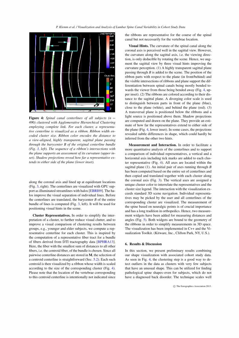
Figure 4: Spinal canal centerlines of all subjects (n =490) clustered with Agglomerative Hierarchical Clusteringemploying complete link. For each cluster, a representa-tive centerline is visualized as a ribbon. Ribbon width en-coded cluster size. Ribbon color encodes the distance toa view-aligned, highly transparent, sagittal plane passingthrough the barycenter B of the original centerline bundle(Fig. 3, left). The sequence of a ribbon’s intersections withthe plane supports an assessment of its curvature (upper in-set). Shadow projections reveal how far a representative ex-tends to either side of the plane (lower inset).

along the coronal axis and lined up at equidistant locations(Fig. 3, right). The centerlines are visualized with GPU sup-port as illuminated streamlines with halos [EBRI09]. The ha-los improve the visual separation of individual lines. Beforethe centerlines are translated, the barycenter B of the entirebundle of lines is computed (Fig. 3, left). It will be used forpositioning visual hints in the scene.

Cluster Representatives. In order to simplify the inter-pretation of a cluster, to further reduce visual clutter, and toimprove a visual comparison of clustering results betweengroups, e.g., younger and elder subjects, we compute a rep-resentative centerline for each cluster. This is inspired bythe computation of a representative fiber tract for a bundleof fibers derived from DTI tractography data [BPHRA13].Here, the fiber with the smallest sum of distances to all otherfibers, i.e. the centroid fiber, of the bundle is chosen. Since allpairwise centerline distances are stored in M, the selection ofa centroid centerline is straightforward (Sec. 5.2). Each suchcentroid is then visualized by a ribbon whose width is scaledaccording to the size of the corresponding cluster (Fig. 4).Please note that the location of the vertebrae correspondingto this centroid centerline is intentionally not indicated since

the ribbons are representative for the course of the spinalcanal but not necessarily for the vertebrae location.

Visual Hints. The curvature of the spinal canal along thecoronal axis is perceived well in the sagittal view. However,the curvature along the sagittal axis, i.e. the viewing direc-tion, is only deducible by rotating the scene. Hence, we aug-ment the sagittal view by three visual hints improving thecurvature perception. (1) A highly transparent sagittal planepassing through B is added to the scene. The position of theribbon parts with respect to the plane (in front/behind) andthe visible intersections of ribbons and plane support the dif-ferentiation between spinal canals being mostly bended to-wards the viewer from those being bended away (Fig. 4, up-per inset). (2) The ribbons are colored according to their dis-tance to the sagittal plane. A diverging color scale is usedto distinguish between parts in front of the plane (blue),close to the plane (white), and behind the plane (red). (3)A transversal plane is positioned below the ribbons and alight source is positioned above them. Shadow projectionsare computed and drawn on the plane. They provide an esti-mate of how far the representatives extend to either side ofthe plane (Fig. 4, lower inset). In some cases, the projectionsrevealed subtle differences in shape, which could hardly beinferred from the other two hints.

Measurement and Interaction. In order to facilitate amore quantitative analysis of the centerlines and to supporta comparison of individual representatives, a vertical and ahorizontal axis including tick marks are added to each clus-ter representative (Fig. 4). All axes are located within thesagittal plane (1). An initial pair of axes running through Bhas been computed based on the entire set of centerlines andthen copied and translated together with each cluster alongthe coronal axis (Fig. 3). The vertical axes are assigned aunique cluster color to interrelate the representatives and thecluster size legend. The interaction with the visualization ex-ceeds standard 3D scene navigation. Individual representa-tives may be picked by the user and all centerlines of thecorresponding cluster are visualized. The measurement ofthe spine based on neuralgic points is of crucial importanceand has a long tradition in orthopedics. Hence, two measure-ment widgets have been added for measuring distances andangles (Fig. 5). Both widgets are bound to the geometry ofthe ribbons in order to simplify measurements in 3D space.The visualization has been implemented in C++ and the Vi-sualization Toolkit. (Kitware, Inc., Clifton Park, NY, U.S.).

6. Results & Discussion

In this section, we present preliminary results combiningour shape visualization with associated cohort study data.As seen in Fig. 4, the clustering step is a good way to de-tect outliers in the data as clusters with very few subjectsthat have an unusual shape. This can be utilized for findingpathological spine shapes–even for subjects, which do nothave a diagnosed back disorder. The technique scales well

c© The Eurographics Association 2013.

P. Klemm et al. / Visualization and Analysis of Lumbar Spine Canal Variability in Cohort Study Data

Figure 5: Interaction facilities. The user may pick a clus-ter representative, i.e. a ribbon, causing the correspondingcluster to be visualized (centerlines with red and yellow ha-los). Widgets for measuring distances and angles facilitate aquantitative analysis of the spinal shape.

regarding the number of input center lines. It is possible togenerate an overview for hundreds of subjects as well as forsmaller subsets, e.g. subjects which share certain similar at-tributes. A subset visualization can be applied to detect ifthe different shape clusters imply a significant difference inassociated variables of interest. Does for example a physicaldemanding job correlate with an extraordinary curved spine?

Our clinical partners expected the lumbar spine to be morestraight along the coronal axis for tall people, while beingmore sinuous ("lordosis") with decreasing body height. Tocheck our results for medical plausibility, we created subsetsof the data based on body height. For each cluster we calcu-lated the distance to the arithmetic mean of age, body height,and weight. We computed the mean of the absolute lordosiscurvatures K using the Frenet formulas [Fre52].

While the mean curvature K for people sized 150 –160 cm is 38.99 · 10−4 (σ = 9.99 · 10−4), it gets smallerthe larger the subjects are, being at 34.59 · 10−4 (σ = 9.98 ·10−4) for 160 – 170 cm and at 31.95 ·10−4 (σ= 8.88 ·10−4)for 180 – 190 cm tall people. We could not only confirmthe expected differences in the distinct groups, but also giveclues for groups which share similar curvature. When look-ing at subject groups of body height 150 – 160 cm, 160– 170 cm and 170 – 180 cm we always found a clusterof subjects which are about 10 years older than the rest ofthe group. They all presented a lordosis shape as well as an"S" shape in sagittal direction ("scoleosis"). Since a cluster

showing the same characteristics was found in distinct sub-ject groups, it is subject of further investigation.

This finding is an example of how a clustering result cancreate groups related by shape in order to find other correla-tions in the associated socio-economic and medical attributeparameters. It can also serve as starting point for a visualanalytics tool to detect risk factors.

The visualization aims for at a visual comparability ofthe clusters. Additionally statistically reliable shape describ-ing features would enhance the method by making statisticalcalculation applicable to deformation information. This canbe achieved by storing the curvature and position of severalfixed points in the FEM model. While the visualization al-lows for characterization of the lumbar spine curvature, it iscurrently not possible to predicate information about spinalcanal narrowings, which can also be an indicator for patholo-gies like spinal stenosis. This is also the case for a vertebraedeformation, which is an indicator for osteoporosis. We planto incorporate such information, e.g, based on an extensionof the finite element model used for spine detection.

7. Conclusion & Future Work

Applying analysis of medical image data associated withnon-image data in a cohort study context is both promis-ing and challenging. The multitude of subjects requires ro-bust yet precise and at least semi-automatic detection andsegmentation algorithms which capture the shape of a struc-ture of interest over a large space of subjects. Assessing theresulting information space demands visualizations, whichmap relevant information among large groups of subjects.

We aim to include more shape describing metrics and ap-ply the technique to all cohort study subjects. This allows fora statistically reliable comparison of clusters. Currently, onlythe overall curvature and torsion is calculated. Those can bemisleading metrics, since coronal as well as sagittal defor-mation can induce a large curvature. The deformation shouldbe class-divided with the analyzed pathology in mind. Thoseand other morphology describing metrics can be transferredto the cohort study data dictionary. We also want to includeinformation about unusual vertebrae alignment.

Our presented approach implements a pipeline for analyz-ing the lumbar spine canal in order to correlate its shape toother variables associated with the cohort study. This wasdone using an association to body height, gender, age andweight. While this was a first step to confirm the expectedshape in different subject groups, it has to be enhanced to beapplicable to all data variables measured in the cohort.

We plan a web-based visual analytics framework thatallows for information visualization on non-image data incombination with complex data set queries including theshape of structures. This allows for possibilities to supportqueries which are not easy to make in classic statistics

c© The Eurographics Association 2013.

P. Klemm et al. / Visualization and Analysis of Lumbar Spine Canal Variability in Cohort Study Data

software, like filtering by geographic location as closenessto the coast. We want to provide the epidemiologists with afast and effective way to analyze their data sets exploitingthe potential which lies beneath the numbers.

Acknowledgements: SHIP is part of the CommunityMedicine Research net of the University of Greifswald,Germany, which is funded by the Federal Ministry ofEducation and Research (grant no. 03ZIK012), the Ministryof Cultural Affairs as well as the Social Ministry of theFederal State of Mecklenburg-West Pomerania. Whole-bodyMR imaging was supported by a joint grant from SiemensHealthcare, Erlangen, Germany and the Federal State ofMecklenburg-Vorpommern. The University of Greifswaldis a member of the ‘Centre of Knowledge Interchange’program of the Siemens AG. This work was supported bythe DFG Priority Program 1335: Scalable Visual Analytics.

References[BBP10] BUSKING S., BOTHA C., POST F.: Dynamic Multi-

View Exploration of Shape Spaces. Computer Graphics Forum29, 3 (2010), 973–982. 2

[BPHRA13] BRECHEISEN R., PLATEL B., HAAR ROMENY B.,A. V.: Illustrative uncertainty visualization of DTI fiber path-ways. The Visual Computer 29, 4 (2013), 297–309. 6

[CGG04] COROUGE I., GOUTTARD S., GERIG G.: Towards ashape model of white matter fiber bundles using diffusion tensormri. In IEEE International Symposium on Biomedical Imaging:Nano to Macro, 2004. (2004), pp. 344–347 Vol. 1. 4

[CLA∗09] CHOU Y.-Y., LEPORÉ N., AVEDISSIAN C., MAD-SEN S. K., PARIKSHAK N., HUA X., SHAW L. M., TRO-JANOWSKI J. Q., WEINER M. W., TOGA A. W., THOMPSONP. M., ALZHEIMER’S DISEASE NEUROIMAGING INITIATIVE:Mapping correlations between ventricular expansion and CSFamyloid and tau biomarkers in 240 subjects with Alzheimer’sdisease, mild cognitive impairment and elderly controls. Neu-roImage 46, 2 (June 2009), 394–410. 2

[CRY11] CABAN J. J., RHEINGANS P., YOO T.: An Evaluationof Visualization Techniques to Illustrate Statistical DeformationModels. Computer Graphics Forum 30, 3 (2011), 821–830. 2

[EBRI09] EVERTS M. H., BEKKER H., ROERDINK J. B., ISEN-BERG T.: Depth-dependent halos: Illustrative rendering of denseline data. IEEE Trans. Vis. Comput. Graphics 15, 6 (2009), 1299–1306. 6

[Fre52] FRENET F.: Sur les courbes à double courbure. Journalde Mathématiques Pures et Appliquées (1852), 437–447. 7

[HSK11] HERMANN M., SCHUNKE A. C., KLEIN R.: Seman-tically steered visual analysis of highly detailed morphometricshape spaces. In BioVis 2011: 1st IEEE Symposium on biologi-cal data visualization (Oct. 2011), pp. 151–158. 2

[HSS∗13] HEGENSCHEID K., SEIPEL R., SCHMIDT C. O.,VÖLZKE H., KÜHN J.-P., BIFFAR R., KROEMER H. K.,HOSTEN N., PULS R.: Potentially relevant incidental findingson research whole-body MRI in the general adult population: fre-quencies and management. European Radiology 23, 3 (2013),816–826. 2, 3

[Kab76] KABSCH W.: A solution for the best rotation to relatetwo sets of vectors. Acta Crystallographica Section A 32, 5 (Sep1976), 922–923. 3

[LCYL08] LIAO W., CHEN H., YANG Q., LEI X.: Analysisof fMRI Data Using Improved Self-Organizing Mapping andSpatio-Temporal Metric Hierarchical Clustering. IEEE Trans-actions on Medical Imaging 27, 10 (2008), 1472–1483. 4

[LTERAC11] LANG-TAPIA M., ESPAÑA-ROMERO V., ANELOJ., CASTILLO M.: Differences on spinal curvature in standingposition by gender, age and weight status using a noninvasivemethod. J Appl Biomech 27, 2 (2011), 143–50. 2

[MM05] MANEK N. J., MACGREGOR A. J.: Epidemiology ofback disorders: prevalence, risk factors, and prognosis. Currentopinion in rheumatology 17, 2 (Mar. 2005), 134–140. 2

[MVvW05] MOBERTS B., VILANOVA A., VAN WIJK J.: Evalu-ation of Fiber Clustering Methods for Diffusion Tensor Imaging.In IEEE Visualization (2005), pp. 65 – 72. 4

[RET13] RAK M., ENGEL K., TÖNNIES K. D.: Closed-FormHierarchical Finite Element Models for Part-Based Object De-tection. In Vision, Modeling, Visualization (2013). 3

[RFS03] RUECKERT D. D., FRANGI A. F. A., SCHNABEL J.A. J.: Automatic construction of 3-D statistical deformationmodels of the brain using nonrigid registration. IEEE Transac-tions on Medical Imaging 22, 8 (July 2003), 1014–1025. 2

[SC04] SALVADOR S., CHAN P.: Determining the Number ofClusters/Segments in Hierarchical Clustering/Segmentation Al-gorithms. In Proc. of Tools with Artificial Intelligence. ICTAI(2004), pp. 576 – 584. 4, 5

[SMvB∗10] STEENWIJK M., MILLES J., VAN BUCHEM M.,REIBER J. H. C., BOTHA C.: Integrated Visual Analysis for Het-erogeneous Datasets in Cohort Studies. Proc. of IEEE VisWeekWorkshop on Visual Analytics in Health Care (2010). 2

[SWST03] SCHULZE-WOLLGAST P., SCHUMANN H., TOMIN-SKI C.: Visual analysis of human health data. International Re-source Management Association, Philadelphia (2003). 2

[TSK05] TAN P.-N., STEINBACH M., KUMAR V.: Introductionto Data Mining. Addison Wesley, 2005. 4

[TYO∗09] TUCER B. B., YALCIN B. M. B., OZTURK A. A.,MAZICIOGLU M. M. M., YILMAZ Y. Y., KAYA M. M.: Riskfactors for low back pain and its relation with pain related disabil-ity and depression in a Turkish sample. Turkish Neurosurgery 19,4 (Sept. 2009), 327–332. 2

[VAS∗11] VÖLZKE H., ALTE D., SCHMIDT C., ET AL.: CohortProfile: The Study of Health in Pomerania. International Journalof Epidemiology 40, 2 (Mar. 2011), 294–307. 1

[vLBK∗13] VON LANDESBERGER T., BREMM S., KIRSCHNERM., WESARG S., KUIJPER A.: Visual analytics for model-basedmedical image segmentation: Opportunities and challenges. Ex-pert Systems with Applications 40, 12 (2013), 4934–4943. 2

[vTKB02] VAN TULDER M., KOES B., BOMBARDIER C.: Lowback pain. Best Practice & Research Clinical Rheumatology 16,5 (2002), 761 – 775. 1, 2

[WP03] WOOLF A. D., PFLEGER B.: Burden of major muscu-loskeletal conditions. Bulletin of the World Health Organization81, 9 (2003), 646–656. 1

[YWSC12] YU H., WANG C., SHENE C.-K., CHEN J. H.: Hier-archical Streamline Bundles. IEEE Transactions on Visualizationand Computer Graphics 18, 8 (2012), 1353–67. 4

[Zag] A. Zagouras. L-method for Com-puting the Optimal Number of Clusters.www.mathworks.com/matlabcentral/fileexchange/37295-l-method/content/Lmethod.m. 5

[ZGP12] ZHANG Z., GOTZ D., PERER A.: Interactive VisualPatient Cohort Analysis. Proc. of IEEE VisWeek Workshop onVisual Analytics in Healthcare, Seattle, Washington (2012). 2

c© The Eurographics Association 2013.

View publication statsView publication stats