Embed Size (px)
Citation preview
Visualization and inference based on wavelet
coefficients, SiZer and SiNos
Cheolwoo Park
Department of Statistics
University of Georgia
Athens, GA 30602-1952
Fred Godtliebsen
Department of Mathematics and Statistics
University of Tromsø
N-9037 Tromsø, Norway
Murad Taqqu
Department of Mathematics and Statistics
Boston University
Boston, MA 02215
Stilian Stoev
Department of Statistics
University of Michigan
Ann Arbor, MI 48109-1107
J. S. Marron
Department of Statistics and Operations Research
University of North Carolina
Chapel Hill, NC 27599-3260
November 18, 2006
1

Summary
SiZer (SIgnificant ZERo crossing of the derivatives) and SiNos (SIgnificant NOnSta-
tionarities) are scale-space based visualization tools for statistical inference. They are
used to discover meaningful structure in data through exploratory analysis involving sta-
tistical smoothing techniques. Wavelet methods have been successfully used to analyze
various types of time series. In this paper, we propose a new time series analysis approach,
which combines the wavelet analysis with the visualization tools SiZer and SiNos. We use
certain functions of wavelet coefficients at different scales as inputs, and then apply SiZer
or SiNos to highlight potential non-stationarities. We show that this new methodology
can reveal hidden local non-stationary behavior of time series, that are otherwise difficult
to detect.
Key words: Internet traffic, Long-range dependence, Non-stationarity, Scale-space method,
SiNos, SiZer, Time series, Wavelet coefficients.
1 Introduction
In a complicated time series, it can be challenging to detect underlying structure. For ex-
ample, Internet traffic data typically have long-range dependence properties, see Leland et
al. (1994), and even non-stationary behavior, see Park et al. (2004). In this context and
in general, it is difficult to distinguish between long-range dependence and non-stationarity.
Some work in this direction includes Teverovsky and Taqqu (1997), Dang and Molnar (1999),
Mikosch and Starica (2000), Rondonotti, Marron, and Park (2004), Giraitis, Kokoszka and
Leipus (2001), Stoev et al. (2006), Veitch and Abry (2001), and Uhlig, Bonaventure, and
Rapier (2003).
In this paper, we propose a new method based on a scale-space approach to detect hid-
den non-stationary behavior of time series which may possess long-range dependence. The
method is capable of tracking both sudden local and gradual changes in the mean, variance
and correlation structure of the time series. Especially, it is very sensitive to sharp local
variations and these variations can be detected on different frequency bands by analyzing
wavelet coefficients. An important advantage of this method is that it can be used to identify
stationary segments of the process as well as localized non-stationary fluctuations. By us-
ing this procedure, one may be able to better understand and possibly explain the observed
behavior in non-stationary regions of the process.
2

Many tools have been developed for the analysis of the long-range dependence structure
of a time series. Some of the most popular ones are, for example, the aggregation of variance
method, see Beran (1994), or Teverovsky and Taqqu (1997), the periodogram based Whit-
tle method, see Robinson (1995), or Taqqu and Teverovsky (1997), and the wavelet based
method, see Abry and Veitch (1998), or Feldmann et al. (1999), Doukhan, Oppenheim, and
Taqqu (2003). Among these, the wavelet methods have been very popular since they allow
us to visualize the scaling behavior of the data (e.g. Internet traffic) as well as to obtain
estimates of the Hurst long-range dependence parameter, see Park et al. (2004) or Abry et
al. (2003). The main idea there is to relate the different wavelet scales in order to estimate
the intensity of long-range dependence, and the Hurst parameter quantifies the degree of
long-range dependence of a time series (see, for example, Beran, 1994). In this paper, we
analyze wavelet coefficients of time series with scale-space methods. The focus of this paper,
is within scale, which is where the decorrelation feature of wavelets comes into play (see Sec-
tion 2.1 for the detail). Each wavelet scale is carefully investigated by scale-space methods
which conduct goodness-of-fit tests.
SiZer (SIgnificant ZERo crossing of the derivatives), which was originally proposed by
Chaudhuri and Marron (1999), combines the scale-space idea of simultaneously considering
a family of smooths (e.g., local linear estimates) with the statistical inference that is needed
for exploratory data analysis in the presence of noise. It brings an immediate insight into
a central scientific issue in exploratory data analysis: which features observed in a smooth
of data are “really” there?. Dependent SiZer, see Park, Marron, and Rondonotti (2004),
extends SiZer to dependent data and provides a goodness of fit test of the underlying time
series model. This can be done by adjusting the statistical inference using an autocovariance
function of the supposed model. Dependent SiZer is particularly useful in the analysis of
Internet traffic data. Indeed, it provides not only visual insights in the structure of these
data but also involves statistical tests for significance of the visually observed features against
those in an assumed noise model.
In addition to the scale-space methods mentioned above, we utilize the SiNos method,
developed by Olsen et al. (2006), to extract information from the wavelet coefficients. SiNos
simultaneously looks for significant changes in the mean, variance, and the first lag autocor-
relation of the observed time series under the null hypothesis that the process is stationary.
Our main idea is to apply SiZer and SiNos to wavelet coefficients of time series, and this
approach enables us to detect a variety of non-stationarities.
The scale-space approach allows for analysis on several time horizons. This is of crucial
3

importance in fields like climatology where the features on time horizons of length one year
and 100 years, respectively, may be very different. The methodology developed in this paper is
therefore very valuable in the analysis of e.g. ice core data from Antarctica. The methodology
is also potentially useful in many other applications, including financial mathematics, speech
recognition, imaging and Internet traffic data. In this paper, we illustrate our methods using
Internet traffic data which have been known to exhibit long-range dependence.
Section 2 describes the details of the wavelet spectrum and scale-space methods. At
the end of this section, a real example analyzed in this paper is introduced. Details and
issues about wavelet coefficient based scale-space methods are provided in Section 3. Real
data analysis, simulation study, and the proposal of a new graphical device summarizing
scale information are presented in Section 4. This new graphical device greatly reduces the
number of plots that must be studied to find significant features, which is very convenient
for exploring multiple time series. Section 5 provides some concluding remarks.
2 Wavelets and scale-space inference
This section describes the wavelet method proposed by Abry and Veitch (1998), and the
SiZer method proposed by Chaudhuri and Marron (1999) and Park, Marron, and Rondonotti
(2004). In addition, a description of SiNos, proposed by Olsen et al. (2006), is given.
2.1 Wavelet spectrum
Here, we briefly review the notion of wavelet spectrum of a time series. We discuss its inter-
pretation and sketch its use for the estimation of the Hurst long-range dependence parameter.
More details and deeper insights can be found in the seminal works of Abry and Veitch (1998),
Veitch and Abry (1999), and Abry et al. (2003).
Consider a discrete time series Y = {Y (i), i = 1, . . . , N}. Using Mallat’s fast discrete
wavelet transform algorithm (see Mallat, 1998) one obtains the set of transformation coeffi-
cients of Y :
{dj,k, k = 1, . . . , Nj}, j = 1, . . . , J,
where Nj ≈ N/2j and J ≈ log2 N . Here, A ≈ B means that the limit of A/B is a constant.
These coefficients are computed efficiently in O(N) operations. The coefficients dj,k can be
4
represented as:
dj,k =∫
RY (t)ψj,k(t)dt, (2.1)
where ψj,k(t) := 2−j/2ψ(2−jt − k), j, k ∈ Z and where Y (t), t ∈ R is a suitable continuous-
time approximation of the time series Y .
The function ψ involved in (2.1) is called an orthonormal mother wavelet. This function
has L zero moments, L ≥ 1, that is
∫tlψ(t)dt = 0, l = 0, 1, . . . , L− 1. (2.2)
It is chosen so that the set of dyadic dilations and integer translations ψj,k(t) = 2−j/2ψ(2−jt−k), j, k ∈ Z of ψ becomes an orthonormal basis of the space L2(dt). The class of Daubechies
wavelets ψ, see for example Daubechies (1992), is particularly useful in practice. These
wavelets have compact support and a number of other important properties. For more details
on the discrete wavelet transform and Mallat’s algorithm see, for example, Ch. 6 in Daubechies
(1992).
In view of (2.1), the coefficient dj,k captures features of the signal Y (t), which match the
time-location (≈ 2jk) and the time-scale (≈ 2j) of the basis function ψj,k. Therefore, the
indices j and k of the dj,k’s are typically called scale and location, respectively. For large j,
the support of ψj,k is wide and consequently the dj,k’s extract coarse scale or low frequency
features of Y (t). Conversely, the wavelet coefficients at small scales j contain fine scale or
high frequency details of the signal.
Suppose now that Y = {Y (i)}i∈Z is a second order stationary random time series. The
wavelet coefficients dj,k of Y reflect naturally its self-similarity and long-range dependence
properties. Indeed, for all j, the time series dj,k, k ∈ Z is stationary and, as j →∞, one has
that
log2
(Ed2
j,k
)∼ j(2H − 1) + C, (2.3)
where C does not depend on j and where H denotes the Hurst long-range dependence expo-
nent of the time series Y . Here A ∼ B means that the limit of A/B is 1. Furthermore, even
though the Y (i)’s can be strongly dependent, in practice, for each fixed scale j the wavelet
coefficients dj,k are essentially uncorrelated in k, i.e., under general conditions on Y , it follows
5

that for sufficiently large fixed j,
Cov(dj,k, dj,k′) = O(|k − k′|2H−1−2L), (2.4)
where L denotes the number of zero moments of the wavelet ψ (see Abry and Veitch, 1998,
and, for example, Stoev et al., 2005). An autocovariance such as (2.4) is summable i.e.∑∞
i=0 |Cov(dj,k, dj,k+i)| < ∞ if L > H. This is in contrast to the long-range dependent
situation where such a sum would diverge (see e.g. Taqqu, 2003).
Using this fact one can estimate well the mean energy Ed2j,k of the wavelet coefficients on
scale j by using sample statistics. Namely, let
Sj := log2
( 1Nj
Nj∑
k=1
d2j,k
)− gNj (j),
where gNj (j) ≈ 1/(ln(2)Nj) is a suitable first order bias correction term (for more details,
see Abry and Veitch, 1998). The statistics Sj are asymptotically unbiased estimators of the
quantities log2(Ed2j,k).
The set of statistics Sj , j = 1, . . . , J is called the wavelet spectrum of the time series
Y (i), i = 1, . . . , N . The wavelet spectrum can be related to the classical Fourier spectrum
of the time series (see Abry and Veitch, 1998, and, for example, Stoev et al., 2005). Large
scales j correspond to low frequency features in the spectral density of Y and therefore the
statistics Sj represent the long-range dependence properties of the data (see (2.3), above).
The statistics Sj for small scales j, however, capture high-frequency features pertinent to the
short term dependence structure of the time series.
In view of (2.3) one can use the wavelet spectrum to estimate the Hurst parameter H.
Indeed, let 1 ≤ j1 < j2 ≤ J and set
H :=( j2∑
j=j1
wjSj + 1)/2,
where∑j2
j=j1wj = 0 and
∑j2j=j1
jwj = 1. Using such weights wj , the estimator H is obtained
from the slope 2H − 1 of a weighted linear regression fit of Sj against j over the range of
scales j1, j1 + 1, . . . , j2. Since (2.3) holds for large j, when estimating the Hurst parameter
H, one focuses on the largest scales of the wavelet spectrum. These scales, however, involve
fewer wavelet coefficients and hence the statistics Sj have greater variability. The choice of
the range of scales [j1, j2] is a subtle problem in the estimation of H. It is partly addressed in
6

Veitch, Abry and Taqqu (2003). More details on the asymptotic statistical properties of H
and other related wavelet-based estimators of the Hurst parameter can be found in Bardet et
al. (2000), Pipiras, Taqqu and Abry (2001), Bardet et al. (2002), and the references therein.
One advantage of the wavelet method is that the vanishing moments property (see (2.2))
makes wavelet spectrum immune to polynomial trends in the data up to order L− 1. Thus,
a smooth, slowly varying trend in a time series is not an issue in the estimation of the Hurst
parameter using the wavelet method as long as L is sufficiently large. Also, Roughan and
Veitch (1999) showed that a smooth enough variation of the mean or variance of the wavelet
coefficients does not impair the estimation of the Hurst parameter.
While the Hurst parameter is important, it is not the only parameter of interest. The
whole range of the wavelet spectrum can carry useful information about the data. In Stoev
et al. (2005), the strengths and the limitations of the wavelet spectrum in Internet traffic
context are explored. As indicated in Section 2.4, one major limitation of the statistics Sj
is that they can average out important time location information contained in the wavelet
coefficients dj,k. To obtain a richer picture, which captures interesting local non-stationarity
features of time series, one should analyze in detail the time series of wavelet coefficients dj,k.
This is done in the following section using natural scale-space smoothing tools such as SiZer
and SiNos.
2.2 SiZer and dependent SiZer
SiZer analysis is a visualization method which enables statistical inference for discovery
of meaningful structure within the data, while doing exploratory analysis using statistical
smoothing methods. In particular, SiZer addresses the question of “which features observed
in a smooth are really there?”, meaning representing important underlying structure, not
artifacts of the sampling noise.
SiZer is based on scale-space ideas from computer vision, see Lindeberg (1994). Scale-
space is a family of kernel smooths indexed by the scale, which is the smoothing parameter or
bandwidth h. SiZer considers a wide range of bandwidths which avoids the classical problem
of bandwidth selection. Furthermore, the target of a SiZer analysis is shifted from finding
features in the “true underlying curve” to inferences about the “smoothed version of the
underlying curve”, i.e. the “curve at the given level of resolution”. The idea is that this
approach uses all the information that is available in the data at each given scale.
7

SiZer visually displays the significance of features over both location x and scale h, using
a color map. It is based on confidence intervals for the derivatives of the underlying curve
and it uses multiple comparison level adjustment. Each pixel shows a color that gives the
result of a hypothesis test for the slope of the smoothed curve, at the point indexed by the
horizontal location x, and by the bandwidth corresponding to the row h. At each (x, h), if the
confidence interval is above (below) 0, which means that the curve is significantly increasing
(decreasing), then that particular map location is colored black (white, respectively). On
the other hand, if the confidence interval contains 0, which means that the curve is not
significantly increasing or decreasing, then that map location is given the intermediate color
of gray. Finally, if there are not enough data points to carry out the test, then no decision
can be made and the location is colored darker gray.
Let us consider a regression problem with a fixed design setting. Given the data (xi, Y (i))
where xi = i/N, for i = 1, . . . , N , a regression problem is described as
Y (i) = g(xi) + εi, (2.5)
where g is a regression function and the εi’s are identically and independently distributed
with E(εi) = 0 and V ar(εi) = σ2 for all i. A time series setting can be viewed as a regression
setting in (2.5) with xi = i. The other difference is that the εi’s are not generally independent.
SiZer applies the local linear fitting method, see e.g. Fan and Gijbels (1996), for obtaining
a family of kernel estimates and derivatives of a regression function. Precisely, at a particular
point x0, the estimates are obtained by minimizing
N∑
i=1
{Y (i)− (β0 + β1(x0 − xi))}2Kh(x0 − xi) (2.6)
over β = (β0, β1)′, where Kh(·) = K(·/h)/h. K is called a kernel function which is usually a
symmetric probability density function. By using a Taylor expansion, it is easy to show that
the solution of (2.6) provides estimates of a regression function and its first derivatives at x0
for different bandwidths, that is β0 ≈ gh(x0) = Kh ∗ g(x0), and β1 ≈ g′h(x0) = K ′h ∗ g(x0)
where ∗ denotes the convolution. More specifically, β = (XT WX)−1XT WY where Y =
8

(Y (1), . . . , Y (n))T , the design matrix of the local linear fit at x0 is
X =
1 (x0 − x1)
1 (x0 − x2)...
...
1 (x0 − xn)
and W = diag{Kh(x0 − xi)}. From this solution, we can construct the family of smooths
parameterized by h and the confidence intervals that underlie the SiZer analysis. These are
of the form
g′h(x0)± q(h)sd(g′h(x0))
where q(h) is an appropriate Gaussian quantile. The significant features are determined
based on whether these confidence intervals are above (below) zero. The details including
the choice of q(h) and the estimation of the standard deviation can be found in Chaudhuri
and Marron (1999). Hannig and Marron (2006) have recently suggested a procedure, using
advanced distribution theory, to improve the multiple comparison tests. We use the updated
version of SiZer in this paper.
SiZer is a useful tool to find meaningful structures in the given data, but its usefulness
can be diminished in the case of dependent data because it assumes independent errors
and compares against a white noise null hypothesis. In cases of dependent data, significant
features appear in SiZer, which are due to the presence of dependence. For correlated data,
Cov(εi, εj) = γ(|i− j|), and the variance of the local polynomial estimator is given by
V (β|X) = (XT WX)−1(XT ΣX)(XT WX)−1
where, for the assumed correlation structure, Σ is the kernel weighted covariance matrix of
the errors where the generic element is given by
σij = γ(|i− j|)Kh(i− i0)Kh(j − i0).
This motivates the need for distinguishing between features due to trends and dependence.
Rondonotti, Marron, and Park (2004) extended SiZer to time series. That method finds
features of the underlying trend function, while taking into account the dependence structure.
Dependent SiZer has a slightly different goal from SiZer for time series. The dependent
SiZer, proposed by Park, Marron, and Rondonotti (2004), uses a true autocovariance function
9
γ of an assumed model instead of estimating it from the observed data. By doing so, a
goodness of fit test can be conducted and we can see how different the behavior of the data is
from that of the assumed model. The only difference between original SiZer and dependent
SiZer is that the latter compares the data with the specified model rather than with white
noise.
Implementation of dependent SiZer requires estimation of the parameters involved in the
autocovariance function. In dependent SiZer, the classical FGN model for the dependence
structure of the underlying time series is adopted. The autocovariance function of FGN, γ is
given by
γ(l) = σ2(|l + 1|2H + |l − 1|2H − 2|l|2H)/2, l = 0, 1, 2, . . . ,
where H, H ∈ (0, 1), is the Hurst long-range dependence parameter and σ2 is the variance
parameter. Thus, one needs to estimate H and σ2 to conduct a goodness of fit test using
dependent SiZer. This parameter estimation is important and detailed discussion of this issue
can be found in Park, Marron, and Rondonotti (2004). The details of the multiple comparison
test procedure in dependent SiZer can be found in Park, Marron, and Rondonotti (2004) and
Rondonotti, Marron, and Park (2004).
2.3 SiNos
The idea in SiNos (Significant Nonstationarities) is to use a sliding window to search for
changes in the mean, variance or first lag autocorrelation of the time series. During this
search, the data in the window are assumed to follow a stationary Gaussian process. A
thorough description of the SiNos method can be found in Olsen et al. (2006).
Let the time series under study be represented by {Y (i), i = 1, ..., N} where Y (i) denotes
the observed value at time point i and N denotes the total number of observations in the
time series. For each chosen scale we define a set of test points along the series. We assume
that θ1 and θ2 denote the true values of either the mean (µ), the variance (σ2), or the first
lag autocorrelation (ρ) in the two windows on each side of a test point. The following null
hypothesis
H0 : θ1 = θ2 against H1 : θ1 6= θ2,
is tested for each of the three parameters at each test point.
10

For a given test point, let
x = (x1,x2) = (x1,1, x1,2, ..., x1,M , x2,1, x2,2, ..., x2,M ) ∈ {Y (t)}
represent the true vector of observations in the two windows, where M denotes the sample
size in each window. When the null hypothesis is correct, the vector x is assumed to be
multinormal. We apply the following test statistics
Tµ(x1,x2) =(x1 − x2)2
s2p
, Tσ2(x1,x2) =s21
s22
, Tρ(x1,x2) =|γ1 − γ2|
s2p
,
where
xi =1M
M∑
j=1
xi,j , s2i =
1M − 1
M∑
j=1
(xi,j − xi)2,
γi =1
M − 1
M−1∑
j=1
(xi,j+1 − xi)(xi,j − xi), i = 1, 2,
denote the ordinary sample estimators for the means, variances and first lag autocorrelation
in the two windows to be compared. Given the null hypothesis, a common variance for the two
windows is assumed and estimated by the pooled estimator s2p = (s2
1 + s22)/2. As illustrated
in Olsen et al. (2006), accurate approximations for tail probabilities of the test statistics can
be found by a saddlepoint method when the vector x is multinormal. Note that this means
that SiNos is searching for changes in the mean, variance and first lag autocorrelation when
the null hypothesis states that the data follow a stationary Gaussian process.
For each window width, numerous tests are performed along the time series. To avoid
a large number of false detections, the method of False Discovery Rate (see Benjamini and
Hochberg, 1995) is used. Another important part of the method is the covariance matrix
estimation. As pointed out in Olsen et al. (2006), the performance of SiNos is good for
a broad range of stochastic processes as long as a reasonable estimate of autocovariance
function can be found. In SiNos, nonparametric estimation of the covariance matrix is used.
For a more detailed discussion of how multiple testing adjustment is taken care of and how
the covariance structure in the dataset is estimated in SiNos, readers are referred to Olsen et
al. (2006).
11

2.4 Illustration based on real data
In the area of Internet traffic analysis, there is a wide range of open research problems
for engineers, computer scientists, probabilists and statisticians. The Poisson process and
exponential distribution have provided a useful workhorse model for the telephone network.
However, it has been shown in a number of places, see e.g. Leland et al. (1994), and Paxon
and Floyd (1995), that the classical queueing theory is inappropriate for the Internet traffic
modeling. A major move away from standard queueing models was taken by a series of papers,
including Paxson and Floyd (1995), Feldmann, Gilbert and Willinger (1998), and Riedi and
Willinger (2000), that was based on the theory originally developed in other contexts by
Mandelbrot (1969), and Taqqu and Levy (1986). Also, several statistical tools have been
developed to explore Internet traffic data, for example, Abry and Veitch (1998), Veitch and
Abry (2001), Uhlig, Bonaventure, and Rapier (2003), Park, Marron, and Rondonotti (2004),
and Stoev et al. (2006). Our goal is to verify non-stationary features from Internet traffic
time series.
In this paper, aggregated traffic is studied via time series of packet counts over bin grids.
Binned time series come from taking the timestamps of individual packets, and reporting the
counts of the number of packets with timestamp values that fall between an equally spaced
grid of bin boundaries in time.
Figure 1 about here.
Figure 1 (a) displays a time series of binned packet counts in Internet traffic coming into
the University of North Carolina, Chapel Hill (UNC). They were measured at the link of
UNC on April 11, Thursday, from 1 p.m. to 3 p.m., 2002 (Thu1300). This time series,
which is the number of packets arriving at the link every 10 milliseconds, can be written
as Y = {Y (i), i = 1, 2, . . . , 726000}. The plot shows several spikes shooting up and down.
Figure 1 (b) displays the wavelet spectrum described in Section 2.1 of the Thu1300 time
series. We used Daubechies wavelets with three zero moments for all wavelet spectra in this
paper. The wavelet spectrum of this time series shows a bump at the scale j = 11. Since the
y–axis of the spectrum corresponds to the energy of the signal at a given scale, this bump
suggests a unusual behavior at j = 11. This has a serious impact on the estimation of the
Hurst parameter (see Stoev et al., 2005, for more details). A serious weakness of the wavelet
spectrum statistics is that they fail to provide information about the time location of the
unusual behavior, because they involve an average through time.
12
Since Internet traffic data are known to exhibit the self-similar property as well as long-
range dependence, see Leland et al. (1994), Fractional Gaussian Noise (FGN) has been a
useful model of Internet traffic time series. Figures 1 (c) and (d) display the dependent SiZer
analysis of the Thu1300 time series. The data are tested against a null hypothesis of FGN
where the Hurst parameter, H, and the variance are 0.9 and 485.6, respectively (see Park,
Marron, and Rondonotti, 2004, for the choice of the parameters). The goal is to see whether
FGN can be used to model the data at large time scales, and if not, to see how far the
data are from FGN. Because FGN is a stationary series, significant features discovered in the
dependent SiZer analysis can be considered as non-stationarities.
The thin curves in Figure 1 (c) display a family of kernel smooths of the Thu1300 time
series. The curve estimates are obtained from the observations, some of which are displayed
as jittered dots in Figure 1 (c). The thin curves correspond to different levels of smoothing,
i.e. bandwidths. The goal of dependent SiZer is to determine which features of the thin
curves are significantly different from those features one would expect to get according to the
assumed FGN model in this example. This is done by constructing the pointwise confidence
intervals of the derivatives of the family of smooths based on the assumed FGN model.
Observe that a sharp valley appears around x = 2500 (seconds). Figure 1 (d) displays the
SiZer map of the data. The horizontal locations in the SiZer map are the same as in the top
panel, and the vertical locations correspond to the same logarithmically spaced bandwidths
that were used for the family of smooths (thin curves) in the top panel. Black (white) colors
in the SiZer map indicate that the thin curves in Figure 1 (c) are significantly increasing
(decreasing, respectively), at the point indexed by the horizontal location and the bandwidth
corresponding to that row, as compared to a FGN model. Intermediate gray colors mean that
the trend shows no increase or decrease that is significantly different from those typical of FGN
at that particular location. The SiZer map in Figure 1 (d) suggests that the valley around
x = 2500 is different from FGN with the given parameters at fine scales. This indication,
however, is not strong in the sense that there are only a few bandwidths (scales) and locations
in the SiZer map where the valley around x = 2500 is flagged as significant. Since dependent
SiZer provides both location and scale information simultaneously, it is very useful to find non-
stationary behavior when a stationary model for the noise is assumed. However, it sometimes
fails to locate non-stationarities that have short durations. Furthermore, the model must be
specified before analyzing the data. Hence, estimation of parameters in the autocovariance
function of the specified FGN model for the noise is additionally needed.
Figures 1 (a)–(d) show that by combining the wavelet spectrum and dependent SiZer, we
13

can find locations where the time series has strong non-stationary behavior. However, there
are serious practical limitations to this approach, caused by the lack of location information
in the wavelet spectrum, by the need to specify an assumed model for the data, and by the
need for parameter estimation in dependent SiZer. In the following section, we propose an
analysis which addresses some of these difficulties.
3 Wavelet coefficient based scale-space methods
Motivated by the idea of combining the wavelet spectrum and dependent SiZer, and by
overcoming the difficulties that they cause, we propose a new visualization tool in this section.
This tool analyzes wavelet coefficients of the data by using the original SiZer, or SiNos tools.
We call these new tools wavelet SiZer and wavelet SiNos, respectively. First, the time series is
decomposed in the wavelet domain and then SiZer or SiNos are applied to each wavelet scale.
The results of statistical inference are indexed by a location parameter k, which is related to
a location in the original time series, and by two scale parameters which are j (frequency)
and h (bandwidth in SiZer) or M (window width in SiNos).
Wavelet SiZer uses functions of wavelet coefficients at different wavelet scales as inputs.
Next, SiZer is used to determine where and how they are significantly different from what
one would have, had the data been stationary. By doing so, wavelet SiZer considers not
only the wavelet coefficients at all scales, but also adds location information at each scale
obtained from SiZer. One advantage, compared to applying dependent SiZer on the raw time
series, is that the conventional SiZer can be used on the wavelet coefficients because they are
essentially uncorrelated (see (2.4) above). This removes the burdens of model specification
and parameter estimation.
In wavelet SiZer, any function f , for example f(x) = |x|p, p > 0, of the wavelet coefficients
{dj,k} in (2.1) of the data can be used as an input for a SiZer analysis. Because wavelet coef-
ficients are short-range dependent even when the original time series is long-range dependent,
as indicated in Section 2.1, it is possible to apply the conventional SiZer to {f(dj,k)}. Thus,
we can use the regression model in (2.5) by slightly modifying it:
f(dj,k) = g(k) + σjεj,k, k ∈ Z, (3.1)
where σj is the standard deviation of f(dj,k) for all j = 1, . . . , [log2(N)]. Here [log2(N)]
means the greatest integer that does not exceed log2(N).
14
We use f(x) = x2 in this paper because it captured the hidden non-stationary behavior
in the variance very well in the examples we considered. This choice is also comparable
to the wavelet spectrum which also involves the squared wavelet coefficients. Sometimes,
other choices of the function f in (3.1) can provide additional insight. For example, the
fourth power of the wavelet coefficients can be useful because it can capture very fine scaling
behavior of the time series by amplifying variations. An example will be presented in Figure
7 in Section 4.
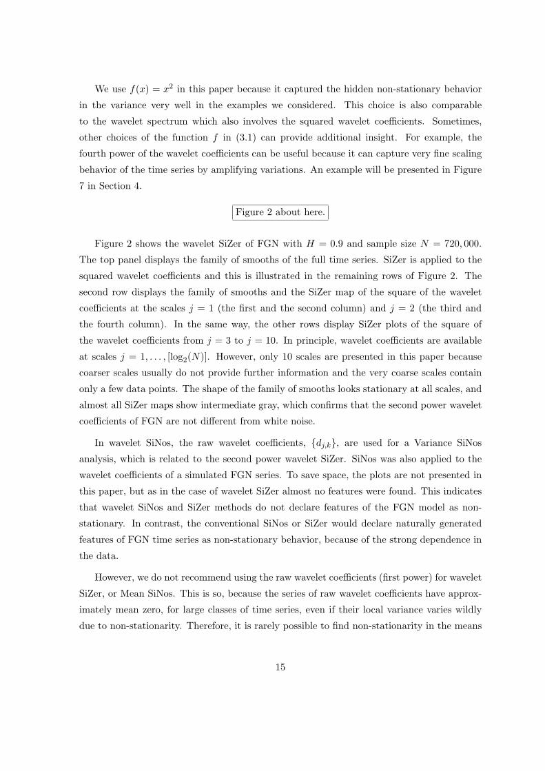
Figure 2 about here.
Figure 2 shows the wavelet SiZer of FGN with H = 0.9 and sample size N = 720, 000.
The top panel displays the family of smooths of the full time series. SiZer is applied to the
squared wavelet coefficients and this is illustrated in the remaining rows of Figure 2. The
second row displays the family of smooths and the SiZer map of the square of the wavelet
coefficients at the scales j = 1 (the first and the second column) and j = 2 (the third and
the fourth column). In the same way, the other rows display SiZer plots of the square of
the wavelet coefficients from j = 3 to j = 10. In principle, wavelet coefficients are available
at scales j = 1, . . . , [log2(N)]. However, only 10 scales are presented in this paper because
coarser scales usually do not provide further information and the very coarse scales contain
only a few data points. The shape of the family of smooths looks stationary at all scales, and
almost all SiZer maps show intermediate gray, which confirms that the second power wavelet
coefficients of FGN are not different from white noise.
In wavelet SiNos, the raw wavelet coefficients, {dj,k}, are used for a Variance SiNos
analysis, which is related to the second power wavelet SiZer. SiNos was also applied to the
wavelet coefficients of a simulated FGN series. To save space, the plots are not presented in
this paper, but as in the case of wavelet SiZer almost no features were found. This indicates
that wavelet SiNos and SiZer methods do not declare features of the FGN model as non-
stationary. In contrast, the conventional SiNos or SiZer would declare naturally generated
features of FGN time series as non-stationary behavior, because of the strong dependence in
the data.
However, we do not recommend using the raw wavelet coefficients (first power) for wavelet
SiZer, or Mean SiNos. This is so, because the series of raw wavelet coefficients have approx-
imately mean zero, for large classes of time series, even if their local variance varies wildly
due to non-stationarity. Therefore, it is rarely possible to find non-stationarity in the means
15

of the raw wavelet coefficients at a given wavelet scale, even when the original signal is non-
stationary. However, non-stationarity in the mean, local variance or local correlations of the
raw data is well–reflected as non-stationarity in the wavelet energy, that is, in the squares
of the wavelet coefficients. Therefore, we focus in this paper, on studying and detecting
non-stationarity in the squares of the wavelet coefficients at a given wavelet scale.
The last issue in wavelet coefficient based scale-space methods is the choice of wavelets.
Daubechies wavelets are typically used because they have compact support and good regu-
larity properties. We use three zero moments in this paper. Different wavelets with different
zero moments result in slight differences in the wavelet SiZer and wavelet SiNos analyses, but
they do not change the main conclusions we draw from the plots.
To save space, we do not report the results in this paper, but the issues discussed in this
section are posted at http://www-dirt.cs.unc.edu/net lrd/wavesizer.html with many
different packet counts traces.
4 Analysis of the Internet traffic data
4.1 Wavelet SiZer and SiNos results
Figure 3 about here.
Figure 3 shows the wavelet SiZer analysis of the Thu1300 time series introduced in Section
2.4. The SiZer plots in Figure 3 at different scales are mostly dominated by four major spikes,
labeled as 1, 2, 3, and 4 in the family of smooths at scale j = 7. Spike 1 appears from j = 1
to j = 5, which are fine wavelet scales. Spike 2 comes up at j = 5 and lasts until j = 10, i.e.
at relatively coarse scales. Note that this spike matches the location that dependent SiZer
had found in Figure 1. Spikes 3 and 4 appear from j = 2 to j = 9, which cover both fine and
coarse scales. Note that spikes 1, 3, and 4 could not be observed in Figure 1, but the wavelet
SiZer is able to reveal these hidden local non-stationarities.
Figure 4 about here.
However, the SiZer maps in Figure 3 do not confirm the significance of all four spikes. For
example, spike 2 is not significant for all j = 5, . . . , 10 according to the SiZer maps although
the smoothing families clearly show the sharp peak. Another scale-space visualization tool
16
which can be combined with wavelet coefficients is SiNos introduced in Section 2.3. Here,
we simply show a plot of the significant changes detected in the Variance SiNos at scale
j = 9 for the Thu1300 data set. In the upper panel of Figure 4, each curve represents an
estimate for the variance of the wavelet coefficients. Different curves correspond to different
degrees of smoothing. The lower panel of Figure 4 shows the feature map for the variance
of the wavelet coefficients. Black, white and gray colors mean increasing, decreasing and no
significant change in the variance respectively. Light gray shows areas where no inference
can be done. This shows the added value of wavelet SiNos, because both peaks are flagged
as significant, while they were not flagged by wavelet SiZer in the lower left part of Figure 3.
More discussion on this issue is presented in Section 5.
Figure 5 about here.
Having found these 4 regions of strong local non-stationarity, it is natural to investigate
them more deeply. To do so, we zoom into the original time series. The four regions high-
lighted as vertical lines in Figure 5 (a) correspond to the locations of the four spikes flagged
as significant by wavelet SiZer in Figure 3. Figures 5 (b), (c), (d), and (e) show the zoomed
time series corresponding to the four windows in Figure 5 (a), respectively. Figure 5 (b)
shows that there is a dropout (absence of signal) for a duration about 0.1 second perhaps
caused by a short router pause, which is a clear type of non-stationarity. Since this dropout
is quickly over with, the spike appears only at fine scales (high frequencies) in wavelet SiZer.
Figure 5 (f) displays the wavelet spectrum for the full time series with this subtrace (shown
in Figure 5 (b)) removed and the remaining two parts concatenated. This does not look
different from the original spectrum in Figure 1 (b), suggesting that this feature does not
cause the bump at j = 11 in the spectrum, therein. Figure 5 (c) shows a long dropout for
about 8 seconds, again a strong local non-stationarity. Since this dropout is much longer
in duration, the spike appears at much coarser scales (low frequencies) in wavelet SiZer in
Figure 3. Figure 5 (g) displays the wavelet spectrum of the full time series with the subtrace
(shown in Figure 5 (c)) removed as for Figure 5 (f), and the bump at j = 11 in Figure 1
(b) disappears. This suggests that the dropout feature plays an important role in causing
the j = 11 bump. Figures 5 (d) and (e) show two unusual drops in both subtraces. Because
the sizes of drops are about half of the size of the signal, this could be caused by one of two
routers pause. Although Figures 5 (h) and (i) display the wavelet spectra of the full time
series with the subtraces (shown in Figure 5 (d) and (e) respectively) removed as above, they
are not different from the original spectrum.
17

Note that since we used the squared wavelet coefficients, these local non-stationarities
are detected in wavelet SiZer and wavelet (Variance) SiNos plots because the time series has
local abnormal changes in the variance rather than it has jump discontinuities. One can
argue that the long dropout in Figure 5 (c) causes the bump at j = 11 in the original wavelet
spectrum, because the bump in Figure 5 (g) is no longer present. Also, additional hidden
non-stationarities were found by wavelet coefficient based visualization tools.
In Figure 3, spikes appear at a number of wavelet scales. This is so because the signal
power of a jump discontinuity, for example, is spread across a wide range of wavelet scales.
Therefore, a jump discontinuity in the mean of the signal results in a non-stationarity (spikes)
of the squares of the wavelet coefficients. We interpret the spikes in the wavelet coefficients
as follows: (i) Spike 1 is an indication of a high frequency, non-stationary disturbance in
the data, since it appears only on relatively fine wavelet scales j = 1 to j = 5. Spike 2
corresponds to a low frequency non-stationarity, since it appears only on the range of scales
j = 5 to 10. Indeed, these observations are confirmed by the analysis in Figures 5 (b) and
(c), where we zoomed into the original time series around the locations of the spikes. (ii)
Spikes 3 and 4 are caused by several variations, some of which are short in duration and some
longer, as seen in Figures 5 (d) and (e). Since these disturbances are located relatively close
to each other, the wavelet coefficients “feel” the non-stationarity over many scales.
Figure 6 about here.
In the Thu1300 data, only spikes are detected by our methods, but sometimes global linear
trends are found, which indicates gradual changes in the variance of the wavelet coefficients.
The top left plot in Figure 6 displays a time series of packet counts, which were measured on
April 12, Saturday, 2003, from 3 p.m. to 4 p.m. (Sat1500). This time series can be written
as Y = {Y (i), i = 1, 2, . . . , 366000}. The series looks rather flat and has less spikes than the
Thu1300 time series in Figure 1 (a). The top right plot shows its family of smooths. The
rest of the plot shows the second power wavelet SiZer of the Sat1500 time series. It shows
increasing trends which correspond to black colors from j = 1 to j = 5, and a dominant spike
extending across scales j = 5 to j = 10.
Figure 7 about here.
In Figure 6, the spike around x = 3000 (seconds) has a similar pattern as the Thu1300
time series in Figure 5. The first window in Figure 7 (a) corresponds to the spike in Figure 6
18

lasting from j = 5 to j = 9. Similar to Figure 5, two drops are observed in the window and
these are displayed in Figure 7 (b). Thus, we confirm that this kind of drop causes a spike
in the second power wavelet SiZer.
Sometimes, other choices of the function f in (3.1) can provide additional insight. Figure
7 (c) shows the SiZer plot of the scale j = 1 with the fourth power, i.e. f(x) = x4, in wavelet
SiZer. Compared to the second power wavelet SiZer in Figure 6, it clearly shows that there
is a spike at the end of the series at j = 1. The second window in Figure 7 (a) corresponds
to this spike and Figure 7 (d) displays the zoomed series corresponding to that window. An
apparent burst behavior is observed in this window. It is of very short duration and is now
flagged as significant because the size of its variation is magnified by taking the fourth power.
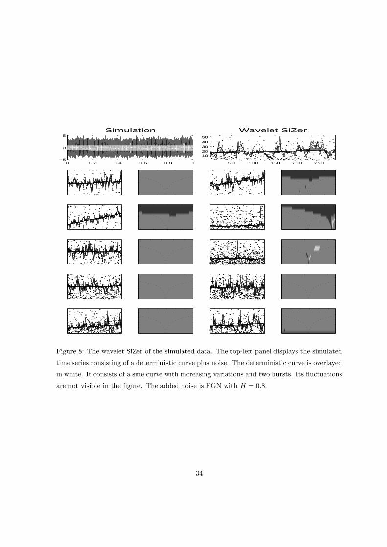
Figure 8 about here.
Having observed spikes or global trends from the scale-space methods in real data, it
would be interesting to explore the possible causation of the phenomena. That is, we would
like to investigate what kind of non-stationarities create spikes and global trends in wavelet
SiZer. Thus, we generated a simulated example, which is displayed in Figure 8. The top left
plot in Figure 8 shows the simulated time series. The underlying trend is a sine curve with
amplitude increasing in time plus two short duration lower frequency sine curves. This trend
is overlayed in white on the plot. The time series is obtained by adding the trend to a FGN
time series with H = 0.8. The trend function is given by
g(xi) = (1 + 0.1xi) sin(0.2πNxi) + sin(0.02πNxi) I(0.5 < xi ≤ 0.507)
+ sin(0.1πNxi) I(0.927 < xi ≤ 0.933),
where xi = i/N for i = 1, . . . , N and N = 300000 is the length of the simulated series.
In other words, the simulated data has a sinusoidal component with increasing amplitude
and two coarse scale bursts around xi = 0.5 and xi = 0.93. This results in a time series
with a gradual non-stationary oscillatory trend and two sharper local non-stationarities.
The increasing amplitude is reflected as an increasing trend in the squares of the wavelet
coefficients on scales j = 2 and 3, in wavelet SiZer. Since the non-stationary oscillatory trend
is of high frequency, the increasing trend in wavelet SiZer is only present at fine scales. On
the other hand, the effect of the two short bursts appears as two spikes at scales j = 4 and
j = 6 in the wavelet SiZer analysis. Since the first burst has lower frequency, it appears at
the coarser scale j = 6, and the second burst has higher frequency, it appears at the finer
19

scale j = 4. Thus, in the wavelet SiZer the increasing fine scale trends could be explained
by this type of increasing magnitude periodic component and the spikes could be caused by
local bursts with particular frequencies that match the scale locations.
These examples suggest that the idea of combining wavelet coefficients and scale-space
methods is a powerful technique for detecting hidden non-stationary behavior of time se-
ries. The types of non-stationarity detected by our tool are related to non-stationarity in
the squares of the wavelet coefficients (or wavelet energy) of the original time series. As
demonstrated, such non-stationarities in the wavelet coefficients can be associated with:
• Sharp, deterministic breaks or shifts in the mean of the data. These appear as spike-like
features in the wavelet coefficients on many wavelet scales.
• Oscillating trends with gradually or sharply changing amplitude. These appear as trends
in the squares of the wavelet coefficients or as spikes. These trends or spikes are found on
wavelet scales, which match the frequencies of the oscillations.
• Because of the use of wavelets, smooth slow deterministic trends cannot be detected if
one uses wavelets with high number of zero moments. They can be detected however with
other existing techniques, for example, dependent SiZer. Our method is particularly suitable
in detecting sudden abrupt changes or subtle stochastic non-stationarities appearing on many
time scales.
• The wavelet spectrum can be related to the Fourier spectrum of a time series. There-
fore, non-stationarity in the squares of the wavelet coefficients can be also related to non-
stationarity in the local covariance structure of the original time series. We therefore believe
that changes in the local second-order dependence structure of the data can be successfully
captured by the wavelet SiZer and wavelet SiNos tools. We plan to investigate this connection
in the future both theoretically and by using simulated examples.
In fact, the new tools enable us to easily find underlying structures in the original time
series that would have been hard to find by simply examining wavelet coefficients. Although
we have focused on Internet traffic data in this paper, the described methodology is also
applicable and useful for other types of time series with potential local non-stationarities.
We analyzed many different packet count traces collected from the UNC link in 2002
and 2003, but we do not report the other results here to save space. However, all results
are displayed and summarized at http://www-dirt.cs.unc.edu/net lrd/wavesizer.html.
We used MATLAB for all plots. As to computation time, it takes around 10 seconds to create
20

a wavelet SiZer plot with N = 300000.
4.2 Summary graphic
Figure 9 about here.
Finally, we propose a new visualization tool for combining inference into a single plot. We
have seen from the presented figures that a major problem with this methodology is that the
user has to analyze and interpret numerous plots for each time series under study. This can,
to some extent, be mitigated by the following approach. In Figure 9, we present a compressed
plot of the information in Figure 3. The upper panel is, as for SiZer, a family plot of the
smooths. In the lower panel we have, however, tried to summarize the important information
of the feature maps in Figure 3 using a gray scale. The horizontal axis shows time while the
vertical axis represents the ten scales from j = 1 to j = 10. For one particular scale and
time, e.g. j = 1 and a specific location on the horizontal axis, we count the number of times
a significant feature appears for this time location in the feature map for j = 1 in Figure 3.
That is, either a significantly increasing (black) or a decreasing (white) trend at this location
is counted as a “significant” feature. We add all significant features up over all bandwidths in
the SiZer map. If there are many (few) significant features for this scale and time in Figure
3, that pixel is colored dark (bright). By examining the plot in Figure 9, we see that it tells
much of the same story as we obtain from all the maps in Figure 3. Of course, it does not
give a detailed description of what is going on, but it certainly indicates that there are local
non-stationarities for many scales and time points. This plot reveals that it is worthwhile
to create and view the detailed plots shown in Figure 3 to learn more about the underlying
structure in the Thu1300 data set. We have also applied this idea to the FGN data set.
The compressed plot for FGN (not shown here to save space) was in this case essentially
white, indicating that it is not necessary to create and view all the feature maps. The idea
of this summary plot approach is simply to disregard automatically those data sets with no
statistically significant behavior. When interesting features are found from this summary
plot, we create wavelet SiZer or wavelet SiNos plot to gain detailed information. This is
an important issue in situations where many data sets are to be analyzed. In addition, it
gives an informative snap shot of the times and scales where potential non-stationarities are
present.
21

5 Discussion
Our main aim in this paper has been to develop tools that use the wavelet spectrum and
wavelet coefficients to detect important features in a time series, and to explore their appli-
cability.
We have adapted two existing scale-space methods to the problem of objectively detecting
significant features in (functions of) the wavelet coefficients. An important lesson is that most
of the features found show up in the squared wavelet coefficients. We therefore focused on
detecting non-stationarity in the second moment (variance) of the wavelet coefficients at a
given scale j. Wavelet SiZer and wavelet SiNos do not rely on a specific dependence model
of the original time series, and yet these tools do not erroneously detect non-stationarity in
strongly dependent data. We calibrated wavelet SiZer and wavelet SiNos over a stationary
long-range dependent FGN time series. Both methods worked well in this case, since as
expected, they did not detect non-stationary features in the squared wavelet coefficients.
When applied to real data (Thu1300, Internet traffic), the two methods give comparable
results with the exception that wavelet SiNos detects some peaks in the squares of the wavelet
coefficients that wavelet SiZer does not flag as significant. We believe that this is due to the
way the present version of SiZer estimates the variance of the test statistic. Preliminary
results (see Hannig and Lee, 2006), using a robust estimator for the variance of this test
statistic, seem promising in the sense that peaks could become easier to detect in this case.
We plan to incorporate the robust SiZer in subsequent versions.
As the referee suggested, the power study of wavelet SiZer and wavelet SiNos would be
an interesting subject, and we propose it as our future work. The thorough power studies of
the original SiZer and its time series version have been well-addressed in Hannig and Marron
(2006), and Rondonotti, Marron, and Park (2004), respectively.
The type of non-stationarity that our tools can detect relates to non-stationarity in the
squares (variance) of the wavelet coefficients of the original data. This analysis has many
advantages since the time series of wavelet coefficients are typically weakly correlated, even
when the data are long-range dependent, and since the wavelet coefficients are capable of lo-
cating features in the data in both frequency and time. Therefore, a possible non-stationarity
in the squares (variance) of the wavelet coefficients reflects changes in the local energy dis-
tribution in the signal, and hence may be attributed to: sharp or oscillating deterministic
trend; shift in the mean; change of the local variance, or, in fact, change in the local covari-
ance structure of the underlying time series. The fact that different wavelet scales correspond
22

to different frequency ranges also allows us to qualitatively interpret the nature and type of
the non-stationarity. More work is necessary to be able to completely understand the scope
of the new tools. We believe however, that our tools can be successfully used to detect subtle
non-stationarity in the data and to also illustrate their statistical nature, by exploring the
data simultaneously in time and frequency domains. In the future, we plan to investigate
further both theoretically and through detailed simulations what is the precise effect of non-
stationarity in the variance of the wavelet coefficients on the local correlation structure of the
data.
Acknowledgments
The Internet traffic data we use here have been processed from logs of IP packets by members
of the DIstributed and Real-Time (DIRT) systems lab at UNC Chapel Hill. Special thanks
are due to Felix Hernandez-Campos. This research was done while Murad S. Taqqu, Fred
Godtliebsen, and Stilian Stoev were visiting the University of North Carolina at Chapel Hill
and the Statistical and Applied Mathematical Sciences Institute (SAMSI) at the Research
Triangle Park. They would like to thank them for providing an excellent environment and
inspiring working atmosphere. This research was also partially supported by the NSF Grants
DMS-0102410 and DMS-0505747 at Boston University.
References
Abry, P. and Veitch, D (1998). Wavelet analysis of long-range dependent traffic. IEEE Trans-
actions on Information Theory, 44, 2–15.
Abry, P., Flandrin, P., Taqqu, M. S. and Veitch, D. (2003). Self-similarity and long-range
dependence through the wavelet lens., in P. Doukhan, G. Oppenheim & M. S. Taqqu, eds,
Theory and Applications of long-range Dependence, Birkhauser, 527–556.
Bardet, J.-M., Lang, G., Moulines, E. and Soulier, P. (2000). Wavelet estimator of long-
range dependent processes. Statistical Inference for Stochastic Processes, 3, 85–99.
Bardet, J.-M., Lang, G., Oppenheim, G., Philippe, A., Stoev, S. and Taqqu, M. (2002).
Semi-parametric estimation of the long-range dependence parameter : A survey, in P. Doukhan,
23
G. Oppenheim & M. S. Taqqu, eds, Theory and Applications of long-range Dependence, Birkhauser,
pp. 527–556.
Benjamini, Y. and Hochberg, Y. (1995). Controlling the false discovery rate: A practical and
powerful approach to multiple testing. Journal of the Royal Statistical Society, Series B, 57,
289–300.
Beran, J. (1994). Statistics for long-memory processes, Chapman & Hall, London.
Chaudhuri, P. and Marron, J. S. (1999). SiZer for exploration of structures in curves. Journal
of the American Statistical Association, 94, 807–823.
Dang, T.D. and Molnar, S. (1999). On the effects of non-stationarity in long-range dependence
tests. Peridica Polytechnica Series on Electrical Engineering, 43(4), 227–250
Daubechies, I. (1992). Ten Lectures on Wavelets, SIAM, Philadelphia.
Doukhan, P., Oppenheim, G., and Taqqu M. S. (2003). Theory and Applications of long-range
Dependence, Birkhauser.
Fan, J., and Gijbels, I. (1996). Local Polynomial Modelling and Its Applications, Chapman &
Hall, London.
Feldmann, A. Gilbert, A. C. and Willinger, W. (1998). Data networks as cascades: inves-
tigating the multifractal nature of Internet WAN traffic. Computer Communication Review,
Proceedings of the ACM/SIGCOMM ’98, 28, 42–55.
Feldmann, A., Gilbert, A. C., Huang, P. and Willinger, W. (1999). Dynamics of IP traffic:
A study of the role of variability and the impact of control. Proceedings of the ACM/SIGCOMM
’99, Boston, MA, 301–313.
Giraitis, L., Kokoszka, P. and Leipus, R. (2001). Testing for long memory in the presence of
a general trend. Journal of Applied Probability, 38(4), 1033–1054.
Hannig, J. and Lee, T. (2006). Robust SiZer for Exploration of Regression Structures and Outlier
Detection. Journal of Computational and Graphical Statistics, 15, 1–17.
Hannig, J. and Marron, J. S. (2006). Advanced Distribution Theory for SiZer. Journal of the
American Statistical Association, 101, 484–499.
Leland, W., Taqqu, M., Willinger, W., and Wilson, D. (1994). On the self-similar nature
of Ethernet traffic. IEEE/ACM Transactions on Networking 2, 1–15.
Lindeberg, T. (1994). Scale Space Theory in Computer Vision, Kluwer, Boston.
Mallat, S. (1998). A Wavelet Tour of Signal Processing, Academic Press, Boston.
24

Mandelbrot, B. B. (1969). Long-run linearity, locally Gaussian processes, H-spectra and infinite
variance. International Economic Review, 10, 82–113.
Mikosch, T. and Starica, C. (2000). Change of structure in financial time series, long-range
dependence and the GARCH model. Center for Analytical Finance, University of Aarhus,
Denmark, Working paper series No 58.
Olsen, L. R., Sørbye, S. H., and Godtliebsen, F. (2006). A scale-space approach for detecting
non-stationarities in time series. To appear in Scandinavian Journal of Statistics.
Park, C., Hernandez Campos, F., Le, L., Marron, J. S., Park, J., Pipiras, V., Smith F.
D., Smith, R. L., Trovero, M., and Zhu, Z. (2004). Long-range dependence analysis of
Internet traffic. Under revision, Technometrics.
Park, C., Marron, J. S. and Rondonotti, V. (2004). Dependent SiZer: goodness of fit tests
for time series models. Journal of Applied Statistics, 31, 999–1017.
Paxson, V. and Floyd, S. (1995). Wide Area traffic: the failure of Poisson modeling. IEEE/ACM
Transactions on Networking, 3, 226–244.
Pipiras, V., Taqqu, M. S. and Abry, P. (2001). Asymptotic normality for wavelet-based esti-
mators of fractional stable motion. Unpublished manuscript.
Riedi, R. and Willinger, W. (2000). Toward an improved understanding of network traffic
dynamics. Self-similar Network Traffic and Performance Evaluation, K. Park and W. Willinger
eds, Wiley, New York, 507–530.
Robinson, P. M. (1995). Gaussian semiparametric estimation of long-range dependence. The
Annals of Statistics, 23, 1630–1661.
Roughan, M. and Veitch, D. (1999). Measuring long-range dependence under changing traffic
conditions. Proceeding of IEEE INFOCOM ’99, 1513–1521.
Rondonotti, V., Marron, J. S., and Park, C. (2004). SiZer for time series: a new approach
to the analysis of trends. Under revison, Journal of Time Series Analysis.
Stoev, S., Taqqu, M., Park, C., and Marron, J. S. (2005). On the wavelet spectrum diagnostic
for Hurst parameter estimation in the analysis of Internet traffic. Computer Networks, 48, 423–
445.
Stoev, S., Taqqu, M., Park, C., Michailidis, G. and Marron, J. S. (2006). LASS: a tool for
the local analysis of self-similarity. Computational Statistics and Data Analysis, 50, 2447–2471.
Taqqu, M. (2003). Fractional Brownian motion and long-range dependence, in Theory and Appli-
cations of Long-range Dependence, P. Doukhan and G. Oppenheim and M. S. Taqqu, editors,
25

Birkhauser, 5–38.
Taqqu, M. and Levy, J. (1986). Using renewal processes to generate LRD and high variability.
Progress in probability and statistics, E. Eberlein and M. Taqqu eds. Birkhaeuser, Boston,
73–89.
Taqqu, M. and Teverovsky, V. (1997). Robustness of Whittle-type estimates for time series
with long-range dependence. Stochastic Models, 13, 723–757.
Teverovsky, V. and Taqqu, M. (1997). Testing for long-range dependence in the presence of
shifting means or a slowly declining trend, using a variance-type estimator. Journal of Time
Series Analysis, 18, 279–304.
Uhlig, S., Bonaventure, O., and Rapier, C. (2003). A graphical wavelet-based method for
analyzing scaling processes. ITC Specialist Seminar, Wurzburg, Germany, 329–336.
Veitch, D. and Abry, P. (1999). A wavelet–based joint estimator of the parameters of long-range
dependence. IEEE Transactions on Information Theory, 45(3), 878–897.
Veitch, D. and Abry, P. (2001). A statistical test for the time constancy of scaling exponents.
IEEE Transactions on Signal Processing, 49, 2325–2334.
Veitch, D., Abry, P. and Taqqu, M. (2003). On the automatic selection of the onset of scaling.
Fractals, 11, 373–390
26

0 2000 4000 60000
100
200
300
400
500
600
700
800
900
1000
(a)
time (sec)
packet
count
s
5 10 159
10
11
12
13
14
15
16
17
18
19
(b)
Scale j
Sj
1842 3684 5526 7368
275
280
285
290
295
300
305
310
315
320
325
(c)
time (seconds)pac
ket co
unts
(d)
time (seconds)
log10(h)
1842 3684 5526 7368
0.5
1
1.5
2
2.5
Figure 1: (a) Time series plot of packet counts measured every 10 milliseconds at the link of
University of North Carolina, Chapel Hill (UNC) on April 11, Thursday, from 1 p.m. to 3
p.m., 2002 (Thu1300). (b) The wavelet spectrum of the Thu1300 time series. The vertical
segments on this plot are the estimated 95% confidence intervals of the log-mean-energy
statistics of the wavelet spectrum. (c) and (d) display the dependent SiZer of the Thu1300
time series. In (d), the dotted curves show effective window widths for each bandwidth, as
intervals representing ±2h.
27

1 2 3 4 5 6 7
x 105
18
20
22
Figure 2: Wavelet SiZer plot of a simulated FGN with H = 0.9. At all scales, the shapes of
the family of smooths look similar.
28

1000 2000 3000 4000 5000 6000 7000
280
300
320
1 2 3 4
Figure 3: Wavelet SiZer plot of the Thu1300 time series. The top panel shows the family of
smooths of the original time series. The second row displays the family of smooths and the
SiZer map of the second power wavelet coefficients at the scales j = 1 and j = 2. In the same
way, the other rows display SiZer plots of the second power wavelet coefficients from j = 3
to j = 10.
29

200 400 600 800 1000 1200 14000
2
4
6
8
10x 10
4 Plot of smooths
estim
ated
Var
(x t)
200 400 600 800 1000 1200 1400 30 40 52 69 91120158208275362478
t
wind
ow w
idth
Variance SiNoS plot
Figure 4: The upper panel is a family plot of Variance SiNos for scale j = 9 of the wavelet
coefficients obtained from the Thu1300 data. The curves show the estimated variance of the
wavelet coefficients for various levels of smoothing. In the lower panel, a feature map showing
significant changes in the variance of the wavelet coefficients, is given.
30

0 1000 2000 3000 4000 5000 6000 70000
200
400
600
800
1000
(a)
time (seconds)
packet
count
s
0 0.5 10
100
200
300
400
500
600
700
(b)
packet
count
s
0 5 100
50
100
150
200
250
300
350
(c)
0 10
100
150
200
250
300
350
400
(d)
0 10 200
100
200
300
400
500
600
700
800
(e)
5 10 15
10
12
14
16
18
(f)
Octave j
yj
5 10 15
10
12
14
16
18
(g)
5 10 15
10
12
14
16
18
(h)
5 10 15
10
12
14
16
18
(i)
Figure 5: (a) Time series plot of the Thu1300 data. The four windows highlighted by the
vertical lines correspond to the significant spikes of the wavelet SiZer in Figure 3. (b), (c), (d),
and (e) show the subtraces corresponding to the four windows in (a), respectively. The units
of the x-axis are seconds. (f), (g), (h), and (i) are corresponding wavelet spectra when each
window is excluded from the full time series and the remaining two parts are concatenated.
31

500 1000 1500 2000 2500 3000 3500
200
400
600
Sat 1500
500 1000 1500 2000 2500 3000 3500450
460
470
480
490
Wavelet SiZer
Figure 6: Wavelet SiZer plot of packet counts measured every 10 millisecond at the link of
University of North Carolina, Chapel Hill (UNC) on April 12, Saturday, from 3 p.m. to 4
p.m. (Sat1500), 2003. The left of the top panel displays the original time series and the right
displays its family of smooths.
32

500 1000 1500 2000 2500 3000 3500
100
200
300
400
500
600
700
(a) Sat 1500
time (seconds)
packet
counts
0 5 10 15
100
200
300
400
500
600
700
(b) Zoomed 1
packet
counts
0 0.1 0.2 0.3 0.4
100
200
300
400
500
600
700
(d) Zoomed 2
time (sec)
packet
counts
5 10 15
x 104
0
5
10
15x 10
6 (c) j=1 (4th order)log 10(h)
0 5 10 15
x 104
3
3.5
4
4.5
5
Figure 7: (a) Time series plot of the Sat1500 data. The first window corresponds to the spike
in wavelet SiZer in Figure 6. (b) shows the subtrace corresponding to the first window in (a).
(c) shows the SiZer plot of scale j = 1 of the fourth power wavelet coefficients. (d) shows the
subtrace corresponding to the second window in (a).
33
0 0.2 0.4 0.6 0.8 1−5
0
5
Simulation
50 100 150 200 250
1020304050
Wavelet SiZer
Figure 8: The wavelet SiZer of the simulated data. The top-left panel displays the simulated
time series consisting of a deterministic curve plus noise. The deterministic curve is overlayed
in white. It consists of a sine curve with increasing variations and two bursts. Its fluctuations
are not visible in the figure. The added noise is FGN with H = 0.8.
34

1000 2000 3000 4000 5000 6000 7000
275
280
285
290
295
300
305
310
315
320
325
(a)
time (second)
(b)
time (second)
j
0 1000 2000 3000 4000 5000 6000 7000
10
9
8
7
6
5
4
3
2
1
Figure 9: The upper panel is a family plot of the Thu1300 time series. The lower panel is a
feature map summary for scales j = 1, 2, . . . , 10 and time points.
35