Visualization of electronic density

Bastien Grossoa,b, Valentino R. Cooperc, Polina Pined, Adham Hashibone,Yuval Yaisha, Joan Adlera,∗

aTechnion-IIT, Haifa, IsraelbEPFL, Lausanne, Switzerland

cOakridge National Laboratory, TN, USAdLoyola University, IL, USA

eFraunhofer IWM, Freiburg, Germany

Abstract

The spatial volume occupied by an atom depends on its electronic density.

Although this density can only be evaluated exactly for hydrogen-like atoms,

there are many excellent algorithms and packages to calculate it numerically

for other materials. Three-dimensional visualization of charge density is chal-

lenging, especially when several levels are intertwined in space. In this paper,

we explore several approaches to this, including the extension of an analglyphic

stereo visualization application based on the AViz package for hydrogen atoms

and simple molecules to larger structures such as nanotubes. We will describe

motivations and potential applications of these tools for answering interesting

physical questions about nanotube properties.

Keywords: visualization, electronic charge density, nanotube

2010 MSC: 00-01, 99-00

THIS is a DRAFT for internal circulation to authors and their supervisors!!

Some technical parts have been moved to appendices.

∗Corresponding authorEmail address: phr76ja@tx.technion.ac.il (Joan Adler)URL: http://phycomp.technion.ac.il (Joan Adler)

Preprint submitted to Journal of LATEX Templates November 4, 2014

1. Introduction and educational applications

The Computational Physics group at the Technion developed a desktop vi-

sualization code for their needs in Atomistic Vizualization, called AViz, [1, 2, 3].5

It is based on Mesa/OpenGL and Qt. Initially we modelled atoms as balls, spins

as cones or vectors and quadrupolar molecules orliquid crystals or pores as cylin-

ders. In a project motivated by educational use we invoked an “off-label” AViz

implementation to illustrate the electric probability density as calulated from

the H atom analytic solution in a smoke rendering form [4], using dots to enable10

semi-transparency. The dot representation of AViz, originally created to enable

quick selection of viewing angle etc for atomistic samples, creates a translucent

effect whereby the sample’s interiors are visible. Combined with color and rota-

tion it gives excellent insight into the nature of the different electronic states[5].

In order to draw the electronic density we (obviously) first need to calculate15

it. In brief, for the H case one calculates the electronic density on a grid, and

defines a box around each grid point. Dots are then drawn at randomly chosen

points within each box at an average density equal to the local electronic density

at the center of the box. Each of these points is given x, y and z coordinates and

is drawn using the dot feature of AViz. The .xyz format is common to many20

molecular visualization packages, but its normally used to indicate atoms, not

density points. For the hydrogen 2s case the datafiles contain some 50,000

points, rather larger than those typically used in atomic visualization, although

since they are not solid spheres, the rendering time is reasonable. In the left

frames of Figure 1 we show the AViz visualization of the electronic density of25

the 2s state of the H atom in both greyscale and color.

Three dimensional visualizations of hydrogen atom wavefunctions are very

helpful for teaching Modern Physics or Quantum Mechanics classes. The con-

cept of electronic density is hard to grasp. Animated gifs of these samples in

rotation are found at [5] using binned color and have been found to be helpful30

to students [6].

2

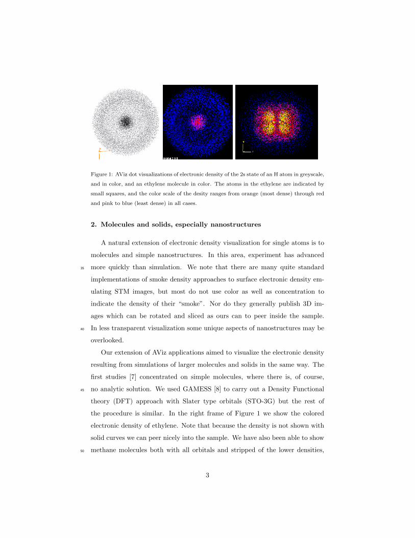
Figure 1: AViz dot visualizations of electronic density of the 2s state of an H atom in greyscale,

and in color, and an ethylene molecule in color. The atoms in the ethylene are indicated by

small squares, and the color scale of the desity ranges from orange (most dense) through red

and pink to blue (least dense) in all cases.

2. Molecules and solids, especially nanostructures

A natural extension of electronic density visualization for single atoms is to

molecules and simple nanostructures. In this area, experiment has advanced

more quickly than simulation. We note that there are many quite standard35

implementations of smoke density approaches to surface electronic density em-

ulating STM images, but most do not use color as well as concentration to

indicate the density of their “smoke”. Nor do they generally publish 3D im-

ages which can be rotated and sliced as ours can to peer inside the sample.

In less transparent visualization some unique aspects of nanostructures may be40

overlooked.

Our extension of AViz applications aimed to visualize the electronic density

resulting from simulations of larger molecules and solids in the same way. The

first studies [7] concentrated on simple molecules, where there is, of course,

no analytic solution. We used GAMESS [8] to carry out a Density Functional45

theory (DFT) approach with Slater type orbitals (STO-3G) but the rest of

the procedure is similar. In the right frame of Figure 1 we show the colored

electronic density of ethylene. Note that because the density is not shown with

solid curves we can peer nicely into the sample. We have also been able to show

methane molecules both with all orbitals and stripped of the lower densities,50

3

and have also explored specific orbitals [7, 9, 10]

Our next attempt at electronic density visualization was to periodically

bounded samples, employed DFT calculations as implemented in the Vienna

Ab Initio Simulation package VASP[11, 12]. In preparation for the larger sam-

ples, we returned to some of the simple molecules with the VASP code. At that55

time we used slice visualization with VESTA [13], since dot visualization for

many atom samples was limited by the very large datafile size issues. Despite

the VESTA solid visualization rather than the 3D dot-smoke type, we confirmed

that the main features agree. Note that VESTA images also include green in

the color range, the early AViz ones only used a red-blue scale for better depth60

perception.

3. Stereo, binned color smoke rendering

The next stage in our visualization development was to move to 3D stereo.

We selected an approach that has a long history, even predating GL. This old

concept of anaglyphic stereo relies on two images, slightly displaced, and viewed65

on a regular screen/projector or poster [14] through colored glasses, or two

squares of cellophane. Stereo Vision (SV) works by showing a different image

to each eye, thus creating the illusion of a 3D image.

AViz 6.1 [15, 16, 17, 18] has incorporated the possibility of SV, and although

more than two colors are possible there remains some color washout, depending70

on color selection. The SV images generated by AViz, such as those in this paper,

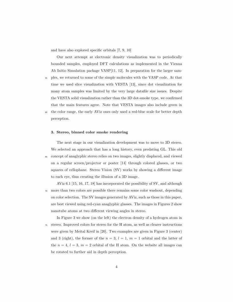
are best viewed using red-cyan anaglyphic glasses. The images in Figures 2 show

nanotube atoms at two different viewing angles in stereo.

In Figure 3 we show (on the left) the electron density of a hydrogen atom in

stereo. Improved colors for stereo for the H atom, as well as clearer instructions75

were given by Meital Kreif in [20]. Two examples are given in Figure 3 (center)

and 3 (right), the former of the n = 3, l = 1, m = 1 orbital and the latter of

the n = 4, l = 3, m = 2 orbital of the H atom. On the website all images can

be rotated to further aid in depth perception.

4

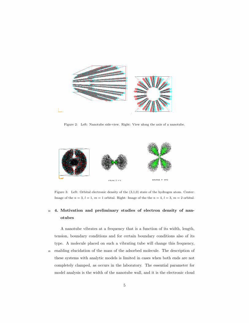
Figure 2: Left: Nanotube side-view. Right: View along the axis of a nanotube.

Figure 3: Left: Orbital electronic density of the (3,1,0) state of the hydrogen atom. Center:

Image of the n = 3, l = 1, m = 1 orbital. Right: Image of the the n = 4, l = 3, m = 2 orbital.

4. Motivation and preliminary studies of electron density of nan-80

otubes

A nanotube vibrates at a frequency that is a function of its width, length,

tension, boundary conditions and for certain boundary conditions also of its

type. A molecule placed on such a vibrating tube will change this frequency,

enabling elucidation of the mass of the adsorbed molecule. The description of85

these systems with analytic models is limited in cases when both ends are not

completely clamped, as occurs in the laboratory. The essential parameter for

model analysis is the width of the nanotube wall, and it is the electronic cloud

5

around the atomic nuclei that determines this.

In a series of papers and a thesis Pine and coworkers [21, 22, 23, 24, 25,90

26, 27] reviewed the literature and carried out extensive classical molecular

dynamics simulations at the atomistic scale to carefully determine the limits

of applicability of the analytic theory. While values for the wall width were

deduced indirectly by us and many others, direct estimation is of course more

desirable. It would be even more desirable to automate this. We are interested95

in the effect of nanotube local distortions (bending, stretching) on the width,

and also in the effect of total strain.

Of course any study to estimate the width directly has to be quantum me-

chanical. Given the limitations of computer resources, and the need for relatively

long tubes, simulated for long times, with a range of parameters it is natural100

that such width estimates should be deduced with a multiscale approach. Sim-

ulations in tandem at an atomistic scale and at an electronic scale are desirable.

The question of multiscale simulations in an efficient manner that minimizes

the difficulty of using diverse codes for different scales, inputs and outputs is

currently an important research issue. For example, in the European Union FP7105

program several collaborations under the banner of “NMP (Nanosciences, Nan-

otechnologies, materials and new production technologies) multiscale modelling”

are researching this issue. In particular the project “Simulation framework for

multiscale phenomena in nano and microscaled systems, or SimPhoNy” [28]

aims towards a uniform environment for scales from electronic to macroscopic,110

with visualization at all scales. The present study, in addition to its intrinsic in-

terest provides a prototype test bed for SimPhoNy. Together with the atomistic

scale and analytic continuum models developed previously, the present study ex-

plores the electronic scale and its visualization development and transfer from

atomistic scale. There is the caveat that the wrapper codes described below are115

C-based and will have to be moved to python for the SimPhoNy environment.

6

4.1. Molecular dynamics as the starting point

The nanotube simulations at the atomistic scale that form the basis for the

present study are described in [22, 23, 24, 25, 26] with codes given in [27].

In brief the tube is equilibrated with periodic boundary conditions, then “cut120

open” and clamped with the appropriate boundary conditions. When strain is

needed the tube is carefully stretched before clamping. It is then allowed to

vibrate for a long time and the vibration spectrum analysed with MATLAB

codes given in [27].

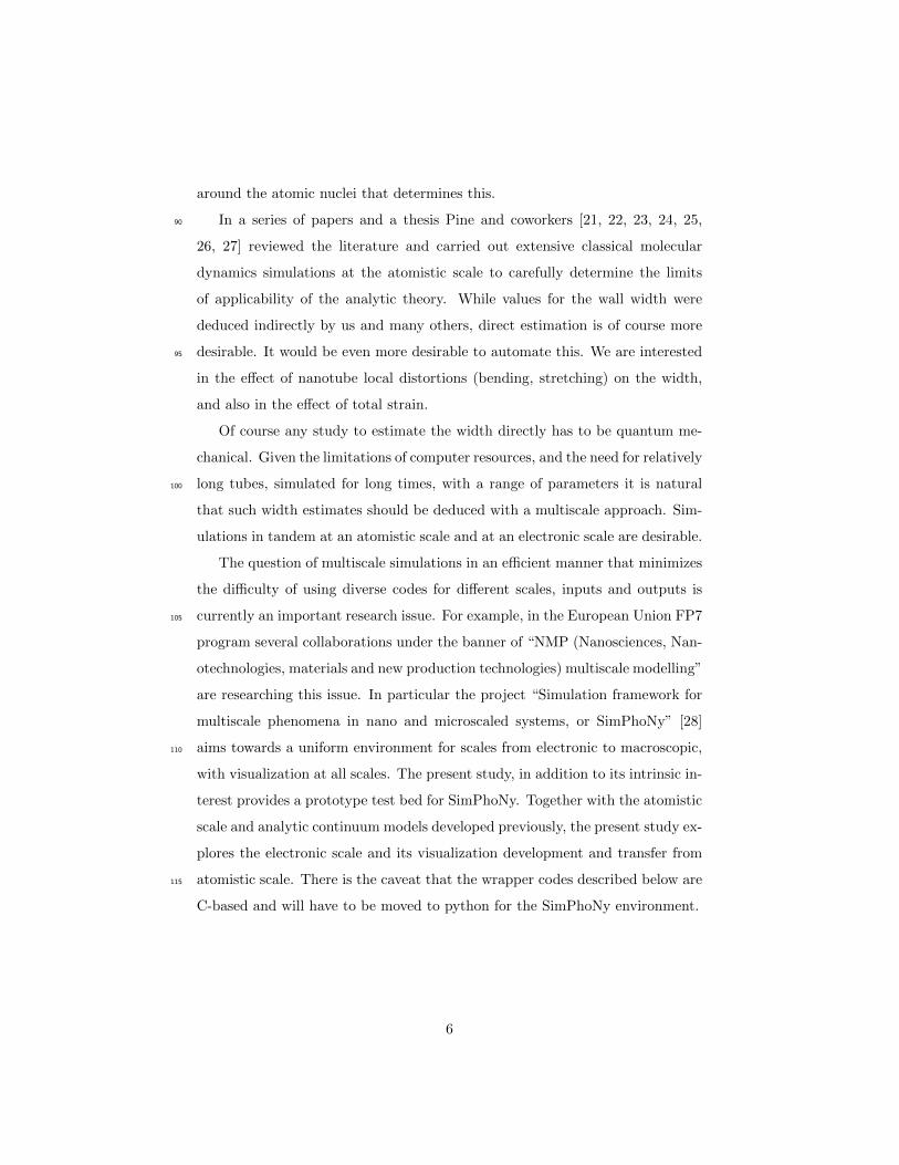
We used the Brenner [30] potential, and for the present study we selected125

four nanotubes with different strains from [26] and used rings near the center

of the tubes so as to minimize boundary effects. We show one of the nanotubes

with 10 percent strain from [26] in Figure 4. Note the slight extension at the

ends to which we will return below. Thoughout this study we refer to the axis

along the tube as the y direction and the two perpendicular dirctions as x and130

z.

Figure 4: Stretched nanotube, the y axis is along the axial direction and xand y directions

are perpendicular; observe extension near the ends.

4.2. Atomistic visualization from molecular dynamics output

For the nanotube simulations we carried out still and animated visualiza-

tion with AViz, creating .xyz files in the simulations and drawing them post-

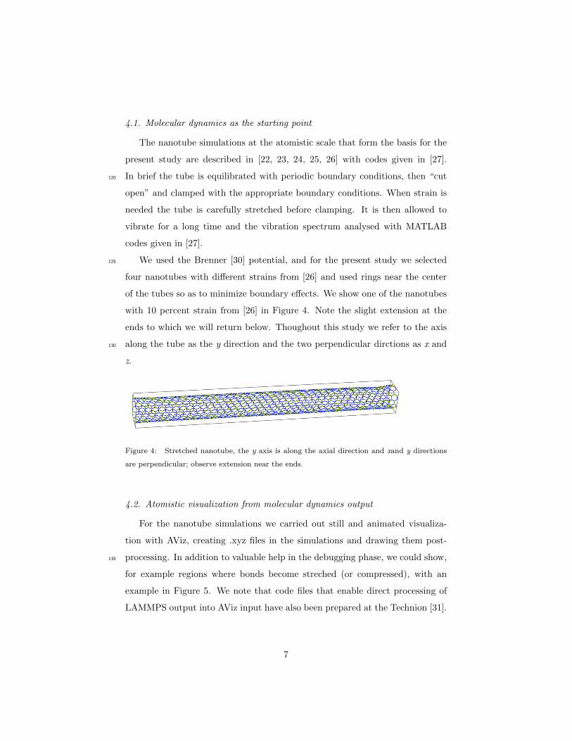
processing. In addition to valuable help in the debugging phase, we could show,135

for example regions where bonds become streched (or compressed), with an

example in Figure 5. We note that code files that enable direct processing of

LAMMPS output into AViz input have also been prepared at the Technion [31].

7

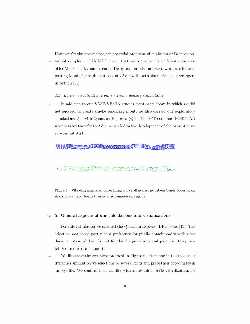
However for the present project potential problems of explosion of Brenner po-

tential samples in LAMMPS meant that we continued to work with our own140

older Molecular Dynamics code. The group has also prepared wrappers for out-

putting Monte Carlo simulations into AViz with both simulations and wrappers

in python [32].

4.3. Earlier visualization from electronic density simulations

In addition to our VASP-VESTA studies mentioned above in which we did145

not succeed to create smoke rendering input, we also carried out exploratory

simulations [34] with Quantum Espresso (QE) [33] DFT code and FORTRAN

wrappers for transfer to AViz, which led to the development of the present more

substantial study.

Figure 5: Vibrating nanotube; upper image shows all nearest neighbour bonds, lower image

shows only shorter bonds to emphasise compression regions.

5. General aspects of our calculations and visualizations150

For this calculation we selected the Quantum Espresso DFT code, [33]. The

selection was based partly on a preference for public domain codes with clear

documentation of their format for the charge density and partly on the possi-

bility of more local support.

We illustrate the complete protocol in Figure 6. From the initial molecular155

dynamics simulation we select one or several rings and place their coordinates in

an .xyz file. We confirm their validity with an atomistic AViz vizualization, for

8

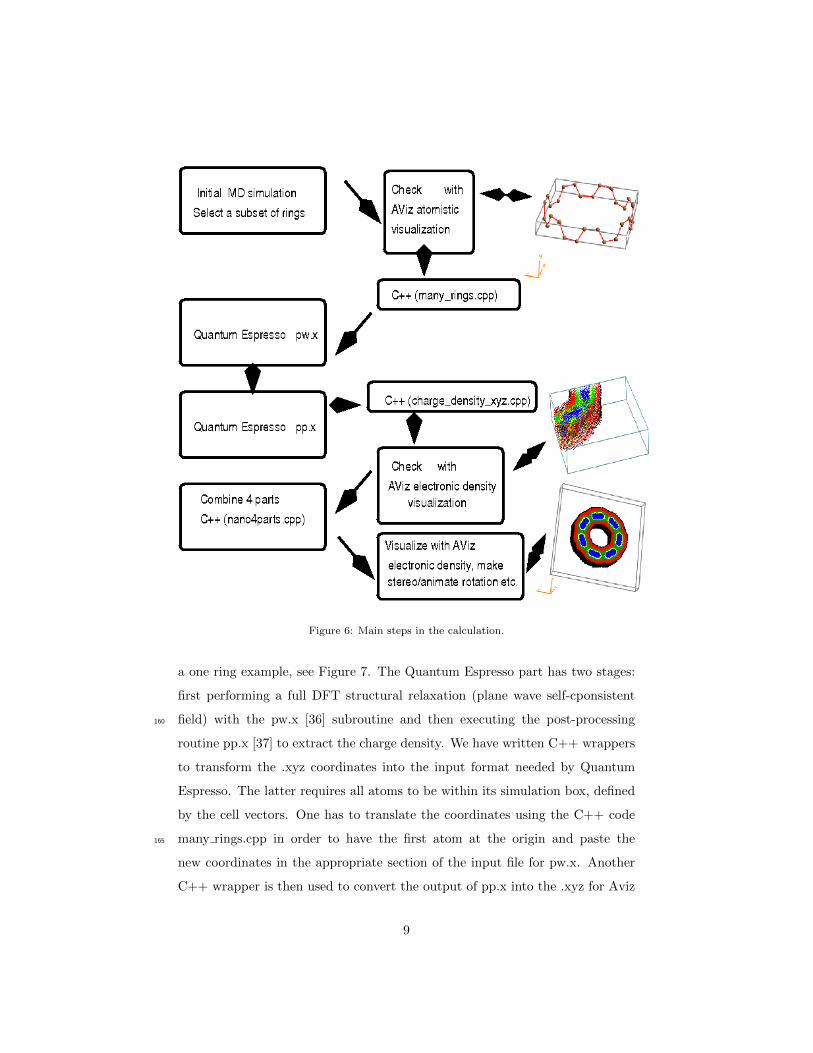
Figure 6: Main steps in the calculation.

a one ring example, see Figure 7. The Quantum Espresso part has two stages:

first performing a full DFT structural relaxation (plane wave self-cponsistent

field) with the pw.x [36] subroutine and then executing the post-processing160

routine pp.x [37] to extract the charge density. We have written C++ wrappers

to transform the .xyz coordinates into the input format needed by Quantum

Espresso. The latter requires all atoms to be within its simulation box, defined

by the cell vectors. One has to translate the coordinates using the C++ code

many rings.cpp in order to have the first atom at the origin and paste the165

new coordinates in the appropriate section of the input file for pw.x. Another

C++ wrapper is then used to convert the output of pp.x into the .xyz for Aviz

9

electronic density visualization. AViz requires an input file in the .xyz format

with two initial rows, the first being the integer number of atoms or dots and

the second a comment line. All other rows have a letter to indicate atomic type170

or dot color and at least three real number spatial coordinates.

All files that we use can be found in a single tar file on the website [35] in

QE charge density/ddl charge density.tar. In addition the input and additional

wrapper routines, currently written in C++ perform the tasks listed below. As

well as being part of the total download file they are also provided as separate175

tar files in the directory QE charge density with the name of the file in brackets

in this list:

• charge density xyz.cpp [35] extracts the charge from pp.x in the correct

input format for AViz (in ddl example input QE.tar)

• many rings.cpp provides the input coordinates for pw.x (in ddl many rings.tar)180

• nano4parts.cpp recombines the 4 quarters into a single ring (in ddl charge density.tar)

(In the current setup QE initially calculates the density in four quadrants

which have to be recombined prior to visualization).

It is also recommended to dilute the points prior to visualization and this is

currently done in this implementation as part of nano4parts.cpp. (This step185

was not needed in the H atom and simple molecule cases because the approach

used to generate points led naturally to a far more dilute concentration.)

We first describe the calculation for a single ring without strain. We then

describe the additional stages needed for systems of several rings and for systems

under strain. The details of the simulations are given in Appendix A, and details190

of the transformations on the output to create AViz input files in Appendix B

and recombination of the 4 parts in Appendix C.

6. Visualization of the charge density in 3D

Once all the steps described above are carried out, we reach the most in-

teresting aspect of this procedure - the visualization of the charge density in195

10

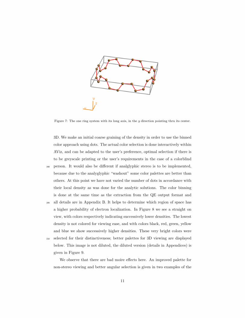
Figure 7: The one ring system with its long axis, in the y direction pointing thru its center.

3D. We make an initial coarse graining of the density in order to use the binned

color approach using dots. The actual color selection is done interactively within

AViz, and can be adapted to the user’s preference, optimal selection if there is

to be greyscale printing or the user’s requirements in the case of a colorblind

person. It would also be different if analglyphic stereo is to be implemented,200

because due to the analyglyphic “washout” some color palettes are better than

others. At this point we have not varied the number of dots in accordance with

their local density as was done for the analytic solutions. The color binning

is done at the same time as the extraction from the QE output format and

all details are in Appendix B. It helps to determine which region of space has205

a higher probability of electron localization. In Figure 8 we see a straight on

view, with colors respectively indicating successively lower densities. The lowest

density is not colored for viewing ease, and with colors black, red, green, yellow

and blue we show successively higher densities. These very bright colors were

selected for their distinctiveness; better palettes for 3D viewing are displayed210

below. This image is not diluted, the diluted version (details in Appendices) is

given in Figure 9.

We observe that there are bad moire effects here. An improved palette for

non-stereo viewing and better angular selection is given in two examples of the

11

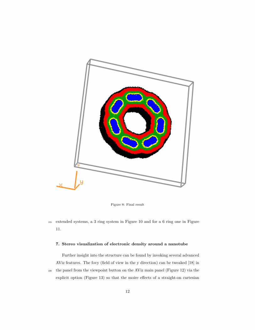
Figure 8: Final result

extended systems, a 3 ring system in Figure 10 and for a 6 ring one in Figure215

11.

7. Stereo visualization of electronic density around a nanotube

Further insight into the structure can be found by invoking several advanced

AViz features. The fovy (field of view in the y direction) can be tweaked [18] in

the panel from the viewpoint button on the AViz main panel (Figure 12) via the220

explicit option (Figure 13) so that the moire effects of a straight-on cartesian

12

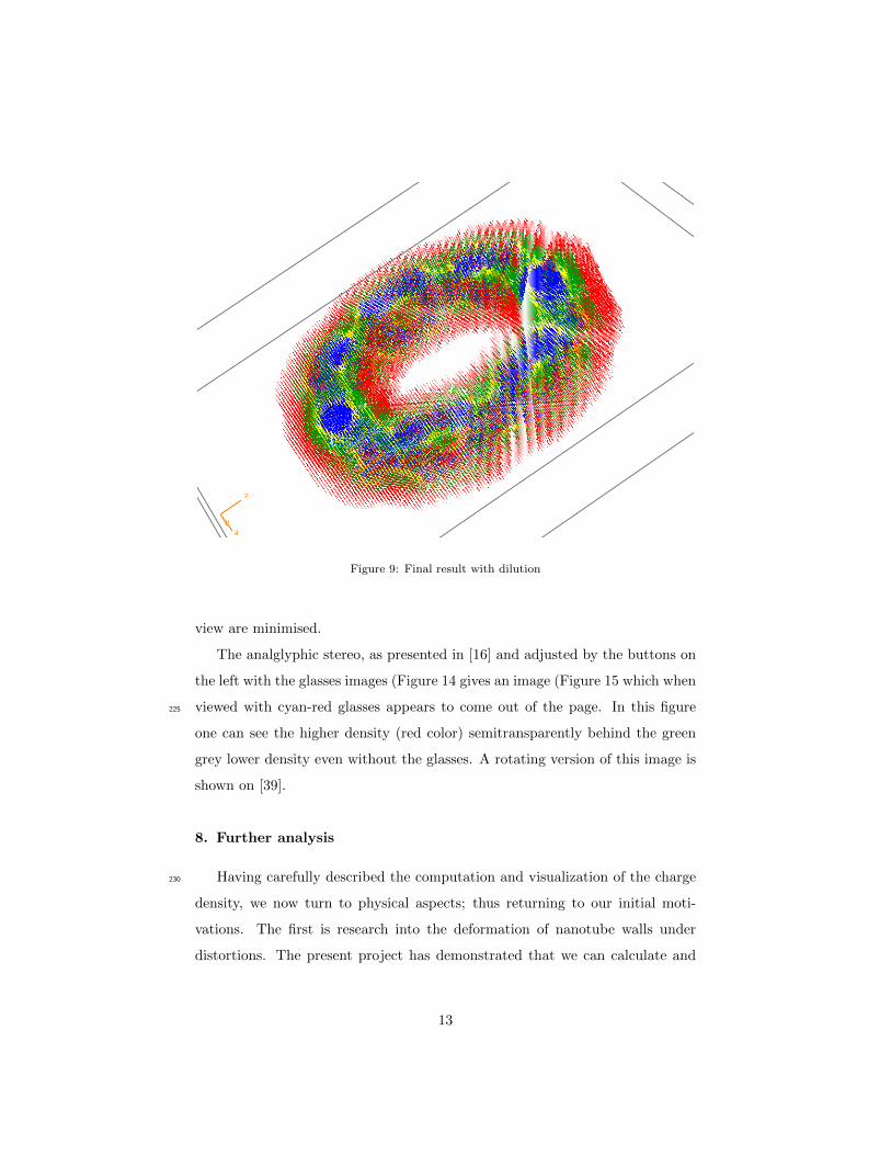
Figure 9: Final result with dilution

view are minimised.

The analglyphic stereo, as presented in [16] and adjusted by the buttons on

the left with the glasses images (Figure 14 gives an image (Figure 15 which when

viewed with cyan-red glasses appears to come out of the page. In this figure225

one can see the higher density (red color) semitransparently behind the green

grey lower density even without the glasses. A rotating version of this image is

shown on [39].

8. Further analysis

Having carefully described the computation and visualization of the charge230

density, we now turn to physical aspects; thus returning to our initial moti-

vations. The first is research into the deformation of nanotube walls under

distortions. The present project has demonstrated that we can calculate and

13

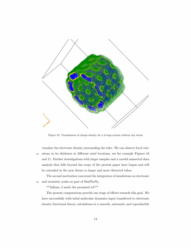
Figure 10: Visualization of charge density for a 3-rings system without any strain

visualize the electronic density surrounding the tube. We can observe local vari-

ations in its thickness at different axial locations, see for example Figures 10235

and 11. Further investigations with larger samples and a careful numerical data

analysis that falls beyond the scope of the present paper have begun and will

be extended in the near future to larger and more distorted tubes.

The second motivation concerned the integration of simulations on electronic

and atomistic scales as part of SimPhoNy.240

**Adham, I await the promised ref.**

The present computations provide one stage of efforts towards this goal. We

have successfully with intial molecular dynamics input transferred to electronic

density functional theory calculations in a smooth, automatic and reproducible

14

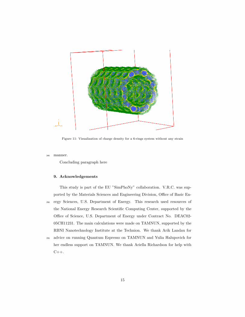
Figure 11: Visualization of charge density for a 6-rings system without any strain

manner.245

Concluding paragraph here

9. Acknowledgements

This study is part of the EU ”SimPhoNy” collaboration. V.R.C. was sup-

ported by the Materials Sciences and Engineering Division, Office of Basic En-

ergy Sciences, U.S. Department of Energy. This research used resources of250

the National Energy Research Scientific Computing Center, supported by the

Office of Science, U.S. Department of Energy under Contract No. DEAC02-

05CH11231. The main calculations were made on TAMNUN, supported by the

RBNI Nanotechnology Institute at the Technion. We thank Arik Landau for

advice on running Quantum Espresso on TAMNUN and Yulia Halupovich for255

her endless support on TAMNUN. We thank Ariella Richardson for help with

C++.

15

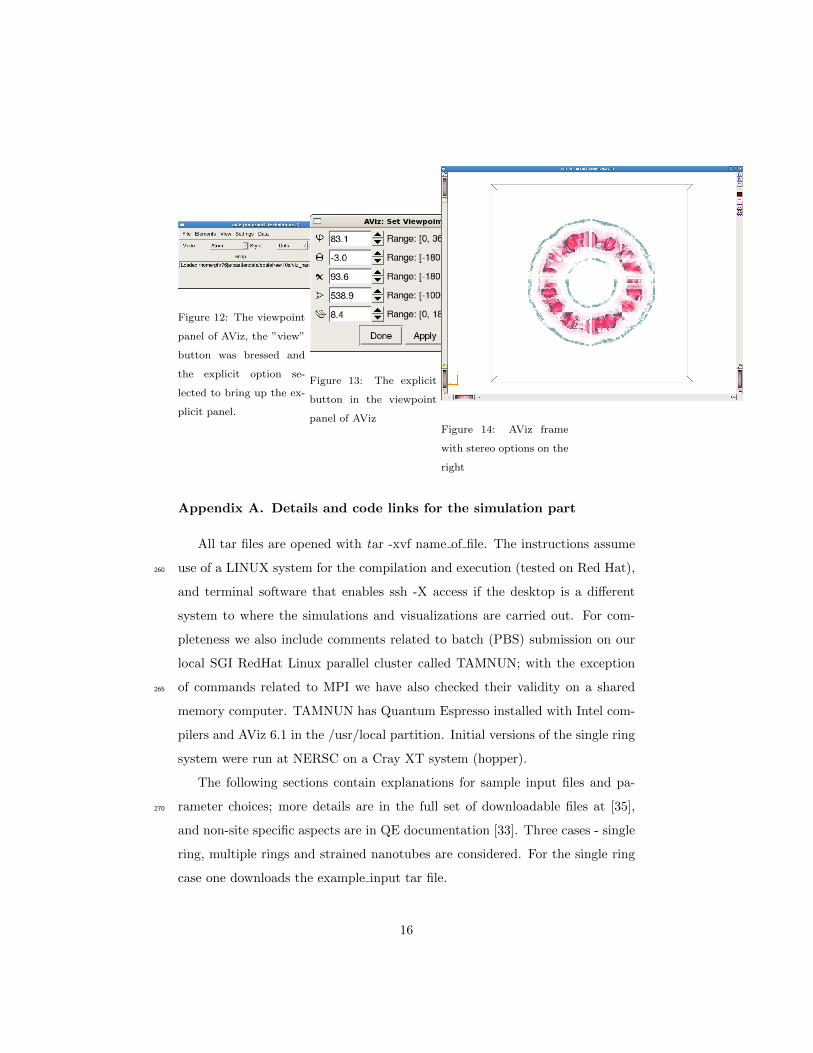
Figure 12: The viewpoint

panel of AViz, the ”view”

button was bressed and

the explicit option se-

lected to bring up the ex-

plicit panel.

Figure 13: The explicit

button in the viewpoint

panel of AVizFigure 14: AViz frame

with stereo options on the

right

Appendix A. Details and code links for the simulation part

All tar files are opened with tar -xvf name of file. The instructions assume

use of a LINUX system for the compilation and execution (tested on Red Hat),260

and terminal software that enables ssh -X access if the desktop is a different

system to where the simulations and visualizations are carried out. For com-

pleteness we also include comments related to batch (PBS) submission on our

local SGI RedHat Linux parallel cluster called TAMNUN; with the exception

of commands related to MPI we have also checked their validity on a shared265

memory computer. TAMNUN has Quantum Espresso installed with Intel com-

pilers and AViz 6.1 in the /usr/local partition. Initial versions of the single ring

system were run at NERSC on a Cray XT system (hopper).

The following sections contain explanations for sample input files and pa-

rameter choices; more details are in the full set of downloadable files at [35],270

and non-site specific aspects are in QE documentation [33]. Three cases - single

ring, multiple rings and strained nanotubes are considered. For the single ring

case one downloads the example input tar file.

16

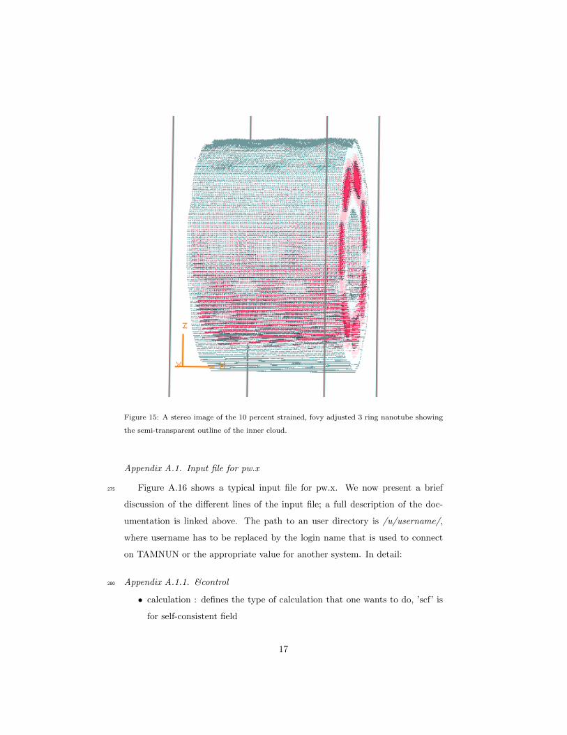
Figure 15: A stereo image of the 10 percent strained, fovy adjusted 3 ring nanotube showing

the semi-transparent outline of the inner cloud.

Appendix A.1. Input file for pw.x

Figure A.16 shows a typical input file for pw.x. We now present a brief275

discussion of the different lines of the input file; a full description of the doc-

umentation is linked above. The path to an user directory is /u/username/,

where username has to be replaced by the login name that is used to connect

on TAMNUN or the appropriate value for another system. In detail:

Appendix A.1.1. &control280

• calculation : defines the type of calculation that one wants to do, ’scf’ is

for self-consistent field

17

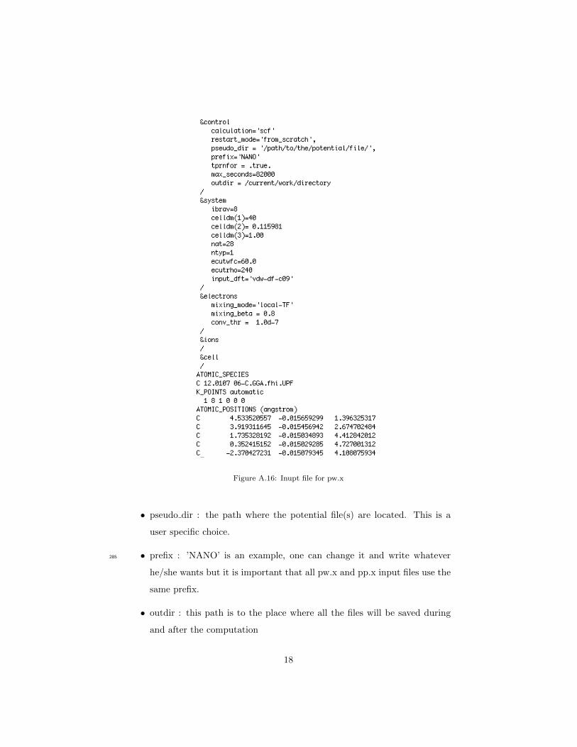
Figure A.16: Inupt file for pw.x

• pseudo dir : the path where the potential file(s) are located. This is a

user specific choice.

• prefix : ’NANO’ is an example, one can change it and write whatever285

he/she wants but it is important that all pw.x and pp.x input files use the

same prefix.

• outdir : this path is to the place where all the files will be saved during

and after the computation

18

Appendix A.1.2. &system290

• ibrav : defines the type of lattice that is used. For example 8 is orthorhom-

bic and depending on the lattice the following lines can change. In the

case of ’ibrav=8’ the basis vectors are given by : v1 = (a, 0, 0), v2 =

(0, b, 0), v3 = (0, 0, c).

• celldm : this part defines the crystallographic constants. An important295

remark is that these values are given in Bohr and not in Angstrom (1

Bohr = 0.529177249 Angstrom). In the orthorhombic case, celldm(1) =

a, celldm(2) = b/a and celldm(3) = c/a. Here an explanation about the

values shown in the example (fig. A.16) is necessary. The vector along

the length of the nanotube is given by celldm(2). The two others are set300

to a big value in order to ”insulate” the system from boundary conditions

effects (celldm(1) = 40, means that a = 40, and celldm(3) = 1, means

that c = 40). To define the value that one has to put for celldm(2), the

way is to measure with a visualization program, the distance between

two consecutive rings, convert this value to Bohr (1 nm = 18.8971 Bohr)305

and divide it by celldm(1), because the measured value will give ’b’, but

celldm(2) = b/a.

• nat : is the number of atoms in the simulation. It has to be equal to the

number of lines under the ”ATOMIC POSITIONS” section.

• ntyp : defines the number of different types of atoms present in the simu-310

lation.

• ecutwfc : is the cutoff for the kinetic energy of the wavefunctions.

• ecutrho : is the cutoff for the kinetic energy of the charge density and

potential, the default value (if not specified) is 4 · ecutwfc.

• :input dft:defines the exchange and correlation functionals employed in the315

calculation. here we cose the vdw-DF non-local correlation functional with

19

the C09x exchange functional in order o account for London dispersion

interactions (or van der Waals forces) within our calculations.

Appendix A.1.3. ATOMIC SPECIES

Under this header one has to specify the type of atom, the mass of the320

atom and the exact name of the pseudopotential that will be used for this atom

(located in ’pseudo dir’).

Appendix A.1.4. ATOMIC POSITIONS

These are the coordinates of the atoms present in the system. There are

many ways to do this; we just specified the type of atom (Carbon in the example325

Figure, A.16) and the coordinates using a .xyz file without the two first lines.

After ATOMIC POSITIONS, we specified the unit (see documentation for more

details). For the structures here we emplyed Cartesion coordinates in angstroms.

Appendix A.2. Run pw.x

Now that the input file is created, one can run pw.x using this input file.330

Using MPI the line to execute the code would be :

mpirun -np n /usr/local/espresso/bin/pw.x < name.in > name.out

where n has to be replaced by the number of processors used. The path before

pw.x is the right one for TAMNUN but could differ on another system. The

result of this first part should be a folder with the name ’prefix’.save, where335

’prefix’ is the name chosen for the prefix, (NANO in our example) and a file

name.out.

Appendix A.2.1. vdw-DF calculations

We have included dispersion(van der Waals) interactions within our DFT

calculations using the van der Walls density function (vdw-DF) [29]. To include340

these interactions in QE it is neccesary to first generate the vdW-DF kernel

table. This can be done using the following procedure:

In this case, the solution is :

20

• copy the file from usr/local/espresso/PW/src generate vdW kernel table.x

into the user’s directory - go into the destination folder and use the com-345

mand (note the . at the end, it is important):

cp usr/local/espresso/PW/src/generate vdW kernel table.x .

• run it with : generate vdW kernel table.x

• move the resulting table file (vdW kermel table) into the directory where350

the pseudopotential is located.

Remark : it can take a moment to execute the generate vdW kernel table.x

file but it only needs to be generated once. (If this is not done properly you

may get:

Error in routine read kernel table (1) :355

No \ ”vdW kernel table \ ” file could be found

If you see this error try again to follow the above directions carefully.)

)

Appendix A.3. Systems of multiple rings

Adding more rings is not totally trivial and should be omitted in a first360

calculation. As explained in section Appendix A.1.2, it is clear that if the

number of rings changes, the number of atoms will change (nat) and the unit

cell length along the c-axis, celldm(2) also change. For example, if the system

is now a 6-rings system the value of celldm(2) has to be multiplied by 6.

The position of the atoms is another aspect that requires care. Indeed, the365

celldm vectors define the simulation box. We recall the values are given in Bohr.

On the other hand, the values of the positions are given in Angstrom. The fact

that the positions are in Angstroms is a special case, it could be defined in

Bohrs if we wanted to. So an important thing to check is that all the atoms

are contained in the volume defined by the celldm vectors. For simplicity our370

box starts from (0,0,0) and has the size of the ’celldm vectors’ values. (Remark

21

: 1 Bohr = 0.5291 Angstrom). So if the atoms are not contained in these

boundaries they have to be translated. To check it, the y-coordinate of the

atom (in Angstrom) has to be in the interval [0, celldm(2) · 0.5291 · celldm(1)].

The atoms just need to be within one unit cell of each other and could be defined375

starting at say (-1/4, -1/4, -1/4).

The translation is done by a script that needs as input file an .xyz file with

the coordinates. After downloading and opening the many rings tar file,

• compile the code with : g++ many rings.cpp -o exec many rings

• put the xyz file in the same folder and execute the code with : ./exec many rings380

• enter the exact name of the file (.xyz included)

• select to do a manual translation or automatic one

A file with the same name plus ” translated.xyz” will be created in the current

directory. These are the new coordinates that will be used.

In the case one chooses to translate automatically, the program will find the385

minimum value in the first and last ring and translate every atom by this value

along the y direction in order to have one atom at the origin and all the others

contained inside of the simulation box.

——————————Valentino and Bastien can you please sort out this

next part—————————————————————390

Appendix A.4. System under strain

The third case that has to be considered with care is the case where there is a

strain in the nanotube. This can also be omitted in a first trial. The consequence

of the strain will be to change the distance between the atoms. When one adds a

strain in the nanotube the distance along y is increased and the distance along395

x and z (direction of the radius) is decreased. As the constraint is constant

the distance between two neighboor-cells along one given direction should be

the same. Nevertheless, as one can probably notice in Figure 4 the slice of

the nanotube does not fall along a perfectly straight line, which means that the

22

distance is not constant everywhere between the consecutive cells. This problem400

is due to the way that the nanotube was built numerically and more specifically

due to the boundary conditions. A way to minimise this problem is to take the

atoms in the middle of the nanotube in order to be as far as possible from the

edges. Every ring has 28 atoms. For the nanotube presented in Figure 4, if

one wants to select a system with 3 rings, the way to select them in the middle405

is to remove the 18 first rings removing the 504 first coordinates, then jump

84 coordinates and remove the rest. One can check that the distance is now

constant between all the atoms. This has been tested for a system of 3 rings

under 2.5, 5 and 10 percent strain. For a larger number of rings this could be

problematic if the distance is not constant.410

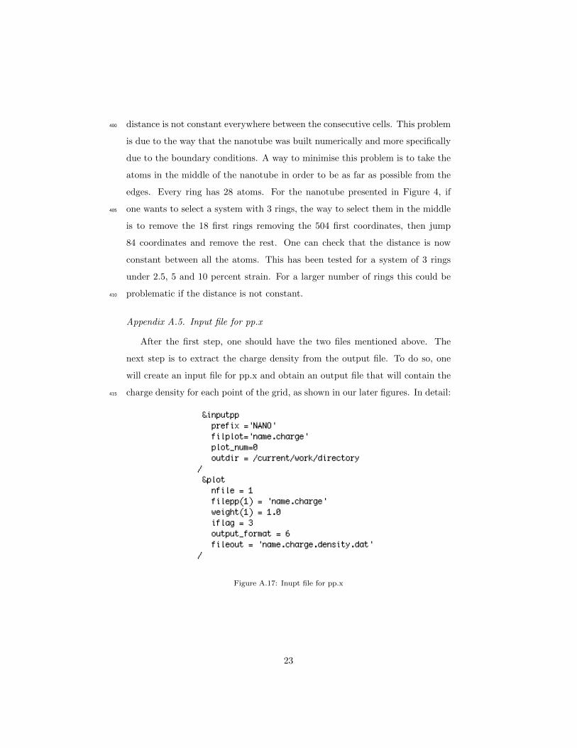
Appendix A.5. Input file for pp.x

After the first step, one should have the two files mentioned above. The

next step is to extract the charge density from the output file. To do so, one

will create an input file for pp.x and obtain an output file that will contain the

charge density for each point of the grid, as shown in our later figures. In detail:415

Figure A.17: Inupt file for pp.x

23

Appendix A.5.1. &inputpp

• prefix : as mentioned before it is really important that the name of the

prefix is exactly the same as it was for pw.x

• filplot : this is the name of the outputfile and can be changed

• plot num : defines the quantity that one is interested in during the post-420

processing, 0 is for the charge density (see the QE documentation for other

values)

• outdir : same as before

Appendix A.5.2. &plot

This section may not be needed for other systems but from our experience425

on TAMNUN it is better to specify it.

• filepp(1) : is the name of the output file that will contain the quantity to

be plotted and saved in fileout, here it is the charge density for example.

• output format : the integer defines the format of the output file (see doc-

umentation).430

• fileout : name of the file that contains the data to do the plot. This is not

used for AViz but it can be useful if one wants to use other software such

as xcrysden [38].

Appendix A.5.3. Remark

On TAMNUN it is important to put the outdir at the end of the section435

&inputpp. An other observation is that it is possible to specify the amount of

data saved during the computation using ’disk io’. If this is not specified the

default value is ’low’ but the less data are saved the more RAM is used and it

can be a problem if the available RAM is not sufficient. The default value is

advised.440

24

Appendix A.6. Run pp.x

The execution line is similar to the previous one :

mpirun -np n /usr/local/espresso/bin/pp.x < name.in > name.out

Appendix A.7. Example of a 1 ring system

For the one ring system (illustrated in Figure 7), the tar contains an input445

file for pw.x and an other one for pp.x and also two bash scripts that create

these files and submit them through the queuing system on TAMNUN.

Appendix A.8. Creation of the .xyz file for the charge density

The output file from pp.x should now be name.charge. This file has the

structure shown in Figure A.18. The first line has 8 numbers, the three first450

numbers are the size of the grid in the three spatial directions, the three following

are the same repeated. The seventh number corresponds to the number of atoms

and the last one to the number of different type of atoms. About the second

line, the first number is the type of Bravais lattice, and the three following

numbers are the celldm defined in the input file of pw.x. The first lines are not455

of interest to us because what we want is the charge density, which is defined

for each point of the grid starting at line 34.

Our aim is to create a .xyz format file with the charge density. More precisely,

each value of charge density given in the output file corresponds to a point in the

grid. To convert this file into an appropriate format one can download a script460

written in C++ as part of the example input file and carry out the following:

1. compile and execute the code : g++ charge density xyz.cpp -o exec charge density

2. copy the file you wish to process into the directory where the script is

3. run ./exec charge density to open the program

4. enter the name of the file to convert and press enter465

A new file with the right format is now created in the same folder and is ready

to be visualized. An older fortran convert file for QE output is at http://

phycomp.technion.ac.il/~aviz/download/download.html.

25

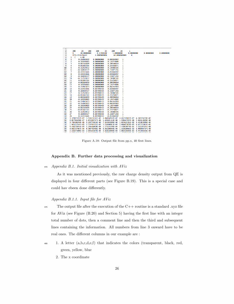
Figure A.18: Output file from pp.x, 40 first lines.

Appendix B. Further data processing and visualization

Appendix B.1. Initial visualization with AViz470

As it was mentioned previously, the raw charge density output from QE is

displayed in four different parts (see Figure B.19). This is a special case and

could hav ebeen done differently.

Appendix B.1.1. Input file for AViz

The output file after the execution of the C++ routine is a standard .xyz file475

for AViz (see Figure (B.20) and Section 5) having the first line with an integer

total number of dots, then a comment line and then the third and subsequent

lines containing the information. All numbers from line 3 onward have to be

real ones. The different columns in our example are :

1. A letter (a,b,c,d,e,f) that indicates the colors (transparent, black, red,480

green, yellow, blue

2. The x coordinate

26

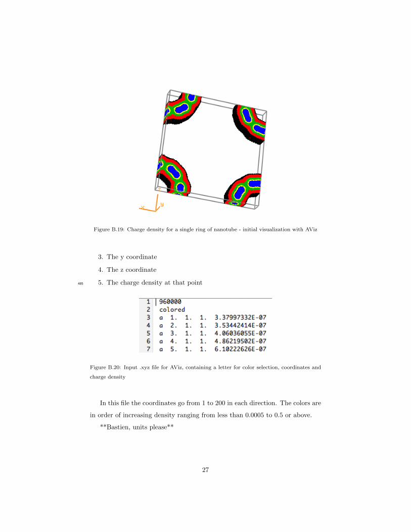
Figure B.19: Charge density for a single ring of nanotube - initial visualization with AViz

3. The y coordinate

4. The z coordinate

5. The charge density at that point485

Figure B.20: Input .xyz file for AViz, containing a letter for color selection, coordinates and

charge density

In this file the coordinates go from 1 to 200 in each direction. The colors are

in order of increasing density ranging from less than 0.0005 to 0.5 or above.

**Bastien, units please**

27

Appendix C. C++ code to recombine the circle

In this part the different important functions implemented will be presented.490

The general procedure is to read the file mentionned above, find which part

corresponds to which quarter of circle, recombine them and create a new input

file for AViz.

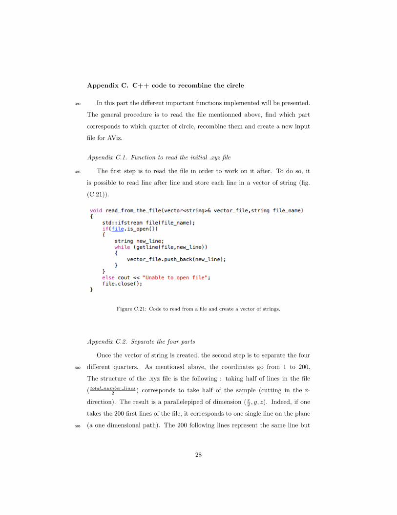
Appendix C.1. Function to read the initial .xyz file

The first step is to read the file in order to work on it after. To do so, it495

is possible to read line after line and store each line in a vector of string (fig.

(C.21)).

Figure C.21: Code to read from a file and create a vector of strings.

Appendix C.2. Separate the four parts

Once the vector of string is created, the second step is to separate the four

different quarters. As mentioned above, the coordinates go from 1 to 200.500

The structure of the .xyz file is the following : taking half of lines in the file

( total number lines2 ) corresponds to take half of the sample (cutting in the z-

direction). The result is a parallelepiped of dimension (x2 , y, z). Indeed, if one

takes the 200 first lines of the file, it corresponds to one single line on the plane

(a one dimensional path). The 200 following lines represent the same line but505

28

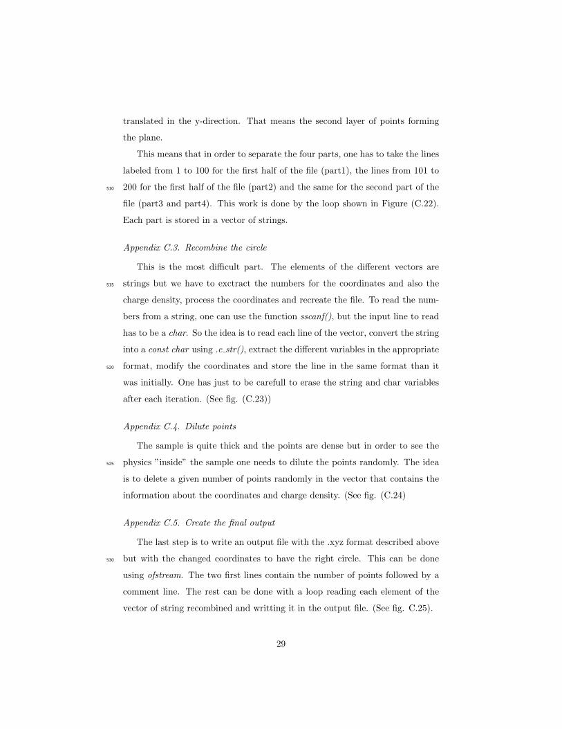
translated in the y-direction. That means the second layer of points forming

the plane.

This means that in order to separate the four parts, one has to take the lines

labeled from 1 to 100 for the first half of the file (part1), the lines from 101 to

200 for the first half of the file (part2) and the same for the second part of the510

file (part3 and part4). This work is done by the loop shown in Figure (C.22).

Each part is stored in a vector of strings.

Appendix C.3. Recombine the circle

This is the most difficult part. The elements of the different vectors are

strings but we have to exctract the numbers for the coordinates and also the515

charge density, process the coordinates and recreate the file. To read the num-

bers from a string, one can use the function sscanf(), but the input line to read

has to be a char. So the idea is to read each line of the vector, convert the string

into a const char using .c str(), extract the different variables in the appropriate

format, modify the coordinates and store the line in the same format than it520

was initially. One has just to be carefull to erase the string and char variables

after each iteration. (See fig. (C.23))

Appendix C.4. Dilute points

The sample is quite thick and the points are dense but in order to see the

physics ”inside” the sample one needs to dilute the points randomly. The idea525

is to delete a given number of points randomly in the vector that contains the

information about the coordinates and charge density. (See fig. (C.24)

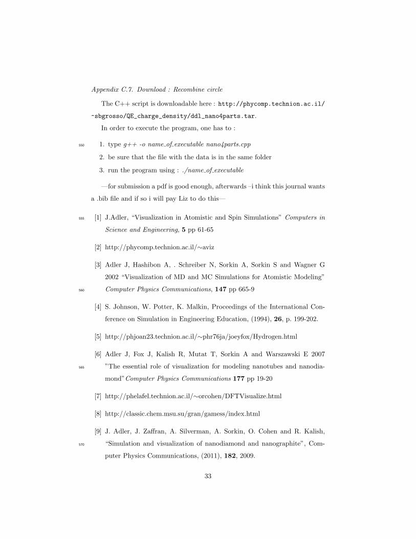
Appendix C.5. Create the final output

The last step is to write an output file with the .xyz format described above

but with the changed coordinates to have the right circle. This can be done530

using ofstream. The two first lines contain the number of points followed by a

comment line. The rest can be done with a loop reading each element of the

vector of string recombined and writting it in the output file. (See fig. C.25).

29

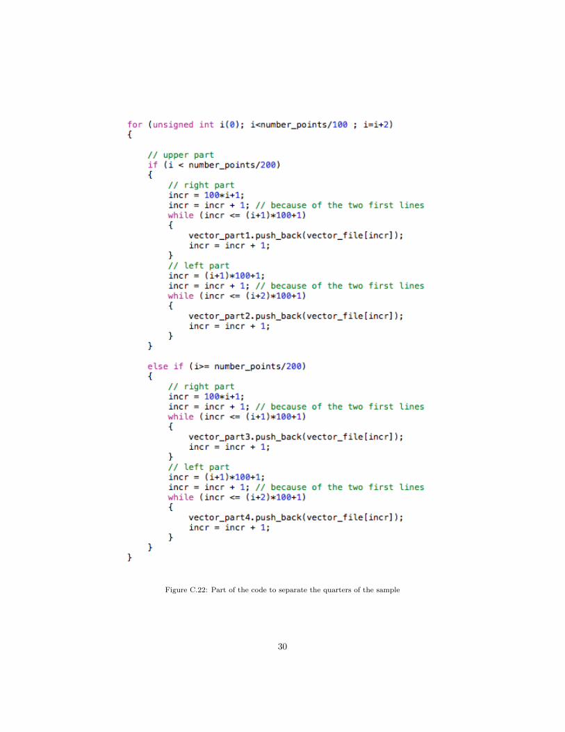
Figure C.22: Part of the code to separate the quarters of the sample

30

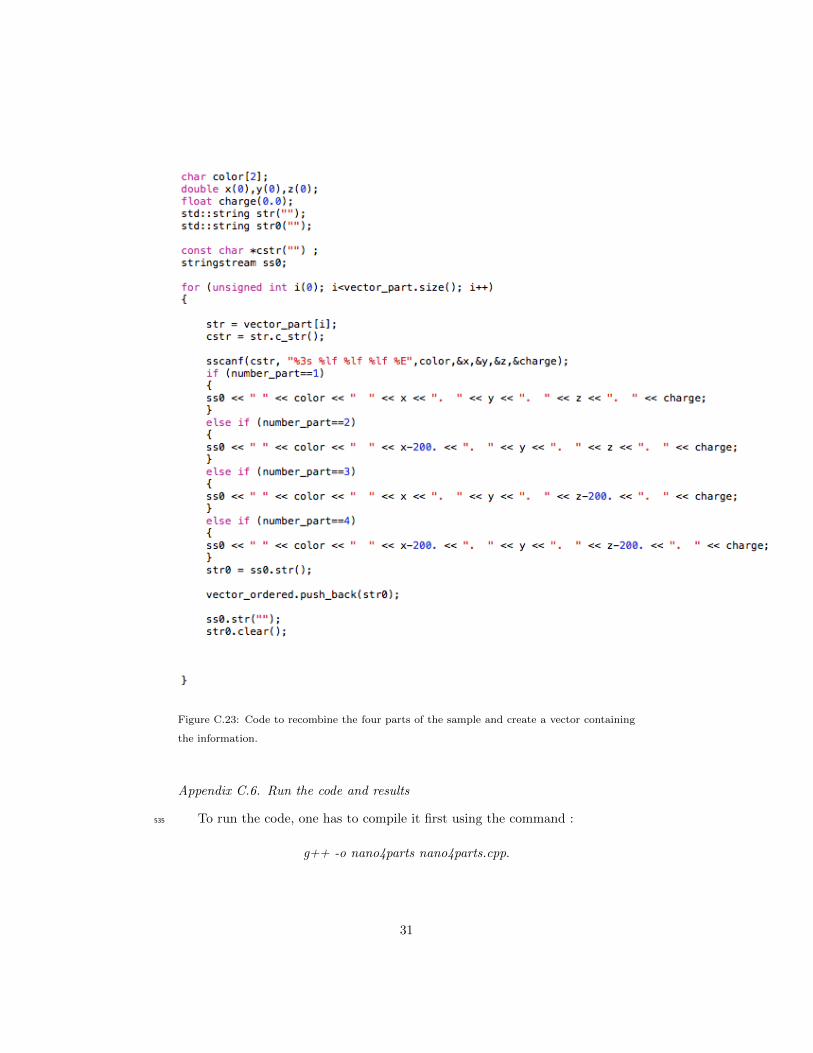
Figure C.23: Code to recombine the four parts of the sample and create a vector containing

the information.

Appendix C.6. Run the code and results

To run the code, one has to compile it first using the command :535

g++ -o nano4parts nano4parts.cpp.

31

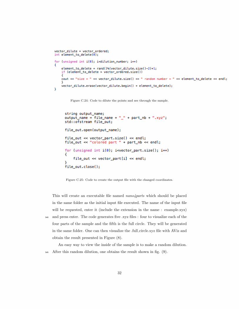
Figure C.24: Code to dilute the points and see through the sample.

Figure C.25: Code to create the output file with the changed coordinates.

This will create an executable file named nano4parts which should be placed

in the same folder as the initial input file executed. The name of the input file

will be requested, enter it (include the extension in the name : example.xyz)

and press enter. The code generates five .xyz files : four to visualize each of the540

four parts of the sample and the fifth is the full circle. They will be generated

in the same folder. One can then visualize the .full circle.xyz file with AViz and

obtain the result presented in Figure (8).

An easy way to view the inside of the sample is to make a random dilution.

After this random dilution, one obtains the result shown in fig. (9).545

32

Appendix C.7. Download : Recombine circle

The C++ script is downloadable here : http://phycomp.technion.ac.il/

~sbgrosso/QE_charge_density/ddl_nano4parts.tar.

In order to execute the program, one has to :

1. type g++ -o name of executable nano4parts.cpp550

2. be sure that the file with the data is in the same folder

3. run the program using : ./name of executable

—for submission a pdf is good enough, afterwards –i think this journal wants

a .bib file and if so i will pay Liz to do this—

[1] J.Adler, “Visualization in Atomistic and Spin Simulations” Computers in555

Science and Engineering, 5 pp 61-65

[2] http://phycomp.technion.ac.il/∼aviz

[3] Adler J, Hashibon A, . Schreiber N, Sorkin A, Sorkin S and Wagner G

2002 “Visualization of MD and MC Simulations for Atomistic Modeling”

Computer Physics Communications, 147 pp 665-9560

[4] S. Johnson, W. Potter, K. Malkin, Proceedings of the International Con-

ference on Simulation in Engineering Education, (1994), 26, p. 199-202.

[5] http://phjoan23.technion.ac.il/∼phr76ja/joeyfox/Hydrogen.html

[6] Adler J, Fox J, Kalish R, Mutat T, Sorkin A and Warszawski E 2007

”The essential role of visualization for modeling nanotubes and nanodia-565

mond”Computer Physics Communications 177 pp 19-20

[7] http://phelafel.technion.ac.il/∼orcohen/DFTVisualize.html

[8] http://classic.chem.msu.su/gran/gamess/index.html

[9] J. Adler, J. Zaffran, A. Silverman, A. Sorkin, O. Cohen and R. Kalish,

“Simulation and visualization of nanodiamond and nanographite”, Com-570

puter Physics Communications, (2011), 182, 2009.

33

[10] http://phycomp.technion.ac.il/∼jeremie

[11] G. Kresse and J. Furthmuller, (1996), Phys. Rev. B 54, 11 169.

[12] G. Kresse and D. Joubert, (1999), Phys. Rev. B. 59, 1758.

[13] http://www.geocities.jp/kmo mma/crystal/en/vesta.html575

[14] Sprott J C “Simple programs create 3D Images” 1992 Computers in Physics

6 pp 132-8

[15] http://phelafel.technion.ac.il/$\sim$peledan

[16] D. Peled, A. Silverman and J. Adler, “3D visualization for atomistic simu-

lations on every desktop”, IOP Conference Series, (2013) 454, p. 012076.580

[17] J. Adler, Y. Koenka and A. Silverman, 2011 “Adventures in carbon visu-

alization with AViz” Physics Procedia 15 pp 7-16

[18] http://phycomp.technion.ac.il/$\sim$newaviz

[19] http://phelafel.technion.ac.il/~meytal

[20] Joan Adler, Yaron Artzi, Liron ben Bashat, Tzipora Yael Izraeli, Meital585

Kreif, Ido Lavi, Alexander Leibenzon, Adam Levi, Itai Schlesinger, Elad

Toledano, Uria Peretz, Yonatan Weisler and Alon Yagil, “How do I simulate

problem X?”, IOP Conference Series, (2014) 510, 012003.

[21] ”Visualization Techniques for Modelling Carbon Allotropes”, J. Adler and

P. Pine, Computer Physics Communications, (2009), 180 , 580-2.590

[22] P. Pine, Y. Yaish and J. Adler, “Simulational and vibrational analysis

of thermal oscillations of single-walled carbon nanotubes”, Phys. Rev. B

(2011), 83, 155410.[/3]

[23] P. Pine, Y. Yaish and J. Adler, “Thermal oscillations of structurally distinct

single-walled carbon nanotubes”, Phys. Rev. B (2011).84,245409.595

34

[24] P. Pine, Y. Yaish and J. Adler, “The affect of boundary conditions on

the vibrations of single-walled carbon nanotubes”, J. App. Phys., (2011),

110, 124311, Also featured in Virtual Journal of Nanoscale Science and

Technology, 25, no 2.

[25] P. Pine, Y. Yaish and J. Adler, “Simulation of nanosensors based on single600

walled carbon nanotubes”, IOP Conference Series, (2012) 402, p.012002.

[26] P. Pine, Y. Yaish and J. Adler, “Vibrational analysis of thermal oscillations

of single-walled carbon nanotubes under axial strain”, PRB, (2014) 89,

115405.

[27] P. Pine, Ph. D. thesis, Technion, 2012, http://phycomp.technion.ac.605

il/~newphr76ja/polina.pdf

[28] http://www.simphony-project.eu

[29] http://pwscf.org/mailman/listinfo/pw_forum

[30] D. W. Brenner, Phys. Rev. B 42, 9458 (1990).

[31] http://phycomp.technion.ac.il/~tamnun/easy_lammps.html610

[32] Joan Adler, Hila Glanz, and Nadir Izrael, “A “Rosetta stone” for AViz”,

Physics Procedia, (2014), 57c pp 2-6. (DOI10.1016/j/phpro.2014.08.122)

[33] http://www.quantum-espresso.org

[34] http://phycomp.technion.ac.il/~tamnun/qe/draw.html

[35] http://phycomp.technion.ac.il/~sbgrosso615

[36] http://www.quantum-espresso.org/wp-content/uploads/Doc/INPUT_

PW.html#idm1680

[37] http://www.quantum-espresso.org/wp-content/uploads/Doc/INPUT_

PP.html

[38] http://www.xcrysden.org/XCrySDen.html620

35

[39] http://phycomp.technion.ac.il/~phr76ja/bastiendata/bastien2.

gif

36