Embed Size (px)
Citation preview
VISUALIZATION OF LARGE SCALE VOLUMETRIC
DATASETS
by
Hamidreza Younesy Aghdam
B.Sc., Sharif University of Technology, Tehran, Iran, 2002
a thesis submitted in partial fulfillment
of the requirements for the degree of
Master of Science
in the School
of
Computing Science
c© Hamidreza Younesy Aghdam 2005
SIMON FRASER UNIVERSITY
Summer 2005
All rights reserved. This work may not be
reproduced in whole or in part, by photocopy
or other means, without the permission of the author.
APPROVAL
Name: Hamidreza Younesy Aghdam
Degree: Master of Science
Title of thesis: Visualization of Large Scale Volumetric Datasets
Examining Committee: Dr. Arthur (Ted) Kirkpatrick, Assistant Professor,
Computing Science, Simon Fraser University
Chair
Dr. Torsten Moller, Assistant Professor,
Computing Science, Simon Fraser University
Senior Supervisor
Dr. Richard Zhang, Assistant Professor,
Computing Science, Simon Fraser University
Supervisor
Dr. Daniel Weiskopf, Assistant Professor,
Computing Science, Simon Fraser University
Supervisor
Dr. Hamish Carr, Lecturer, Computer Science, Uni-
versity College Dublin
External Examiner
Date Approved:
ii
Abstract
In this thesis, we address the problem of large-scale data visualization from two aspects,
dimensionality and resolution. We introduce a novel data structure called Differential Time-
Histogram Table (DTHT) for visualization of time-varying (4D) scalar data. The proposed
data structure takes advantage of the coherence in time-varying datasets and allows efficient
updates of data necessary for rendering during data exploration and visualization while
guaranteeing that the scalar field visualized is within a given error tolerance of the scalar
field sampled.
To address the high-resolution datasets, we propose a hierarchical data structure and
introduce a novel hybrid framework to improve the quality of multi-resolution visualization.
For more accurate rendering at coarser levels of detail, we reduce aliasing artifacts by ap-
proximating data distribution with a Gaussian basis at each level of detail and we reduce
blurring by using transparent isosurfaces to capture high-frequency features usually missed
in coarse resolution renderings.
iii
I dedicate this work to my parents
for their unconditional love and continuous supports
iv
“Let the beauty of what you love be what you do.”
— Jalal ad-Din Rumi (Persian Poet and Mystic, 1207-1273)
v
Acknowledgments
I would like to express my deepest gratitude to my supervisor Dr. Torsten Moller whose
expertise, inspiring ideas, understanding, and patience, added considerably to my graduate
experience.
I would like to thank the other members of my committee, Dr. Hamish Carr for his
generous support and invaluable remarks on my work, and to Dr. Richard Zhang and Dr.
Daniel Weiskopf for the assistance they provided at all levels of the research project.
Many thanks to Dr. Arman Rahmim, Hamidreza Vajihollahi, and my colleagues and
friends at Simon Fraser University and GrUVi Lab for their assistance on countless occasions,
exchanges of knowledge, and venting of frustration during my graduate program, which
helped enrich the experience.
Finally, I wish to thank my parents and family in Iran for all the sacrifices and support
they provided me through my entire life.
vi
Contents
Approval ii
Abstract iii
Dedication iv
Quotation v
Acknowledgments vi
Contents vii
List of Tables ix
List of Figures x
1 Introduction 1
2 State of the Art 5
2.1 State of the Art in Time-Varying Data Visualization . . . . . . . . . . . . . . 5
2.2 State of the Art in Multi-resolution Techniques . . . . . . . . . . . . . . . . . 7
3 Visualization of Time-Varying Volumetric Data 9
3.1 Data Characteristics . . . . . . . . . . . . . . . . . . . . . . . . . . . . . . . . 10
3.2 Case Studies: Data Characteristics of Isabel & Turbulence . . . . . . . . . . . 12
3.2.1 Temporal Coherence . . . . . . . . . . . . . . . . . . . . . . . . . . . . 12
3.2.2 Histogram Distribution . . . . . . . . . . . . . . . . . . . . . . . . . . 13
3.2.3 Spatial Distribution . . . . . . . . . . . . . . . . . . . . . . . . . . . . 15
vii
3.3 Differential Time-Histogram Table . . . . . . . . . . . . . . . . . . . . . . . . 15
3.3.1 Computing the DTHT . . . . . . . . . . . . . . . . . . . . . . . . . . . 15
3.3.2 Queries in the DTHT . . . . . . . . . . . . . . . . . . . . . . . . . . . 24
3.4 Results and Discussion . . . . . . . . . . . . . . . . . . . . . . . . . . . . . . . 25
4 Multi-resolution Volume Rendering 36
4.1 Rendering . . . . . . . . . . . . . . . . . . . . . . . . . . . . . . . . . . . . . . 38
4.1.1 Accurate Multi-resolution Transfer Functions . . . . . . . . . . . . . . 38
4.1.2 Translucent Isosurfaces . . . . . . . . . . . . . . . . . . . . . . . . . . 42
4.1.3 Combined Isosurface and Volumetric Rendering . . . . . . . . . . . . . 43
4.1.4 Progressive Refinement Using Image Caches . . . . . . . . . . . . . . . 44
4.2 Hybrid Branch-on-Need Octree (HYBON) . . . . . . . . . . . . . . . . . . . . 45
4.2.1 Hybrid Octree Representation . . . . . . . . . . . . . . . . . . . . . . . 45
4.2.2 Hybrid Octree Optimization . . . . . . . . . . . . . . . . . . . . . . . . 48
4.3 Implementation and Results . . . . . . . . . . . . . . . . . . . . . . . . . . . . 49
4.3.1 Memory and storage overhead . . . . . . . . . . . . . . . . . . . . . . . 51
5 Conclusions and Future Work 74
5.1 Future Work . . . . . . . . . . . . . . . . . . . . . . . . . . . . . . . . . . . . 75
Bibliography 76
viii
List of Tables
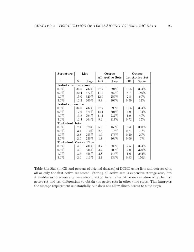
3.1 Size (in GB and percent of original dataset) of DTHT using lists and octrees
with all or only the first active set stored. Storing all active sets is expensive
storage-wise, but it enables us to access any time step directly. As an alter-
native we can store only the first active set and use differentials to obtain
the active sets in other time steps. This improves the storage requirement
substantially but does not allow direct access to time steps. . . . . . . . . . . 23
ix
List of Figures
3.1 Temporal Coherence: Number of samples that change by more than an error
bound of λ = 0%, 0.3%, 1%, 3% for the temperature and pressure scalars of
the Isabel dataset as well as the jets and vortex datasets. . . . . . . . . . . . 14
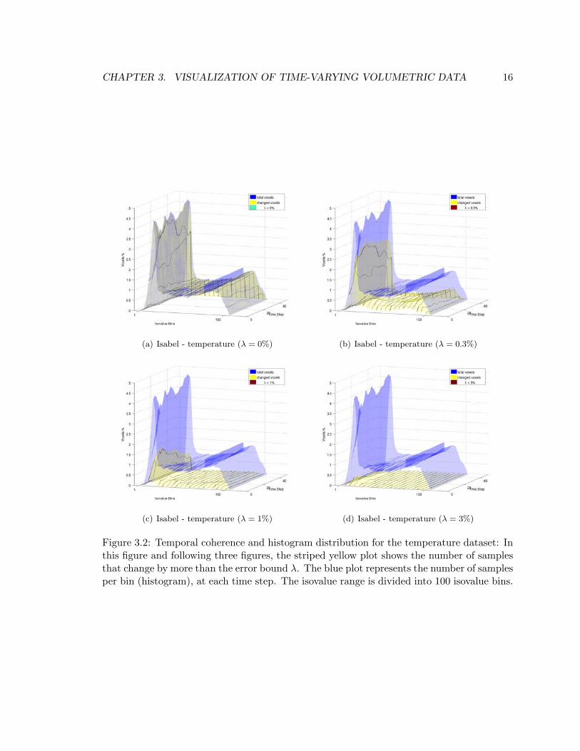
3.2 Temporal coherence and histogram distribution for the temperature dataset:
In this figure and following three figures, the striped yellow plot shows the
number of samples that change by more than the error bound λ. The blue
plot represents the number of samples per bin (histogram), at each time step.
The isovalue range is divided into 100 isovalue bins. . . . . . . . . . . . . . . 16
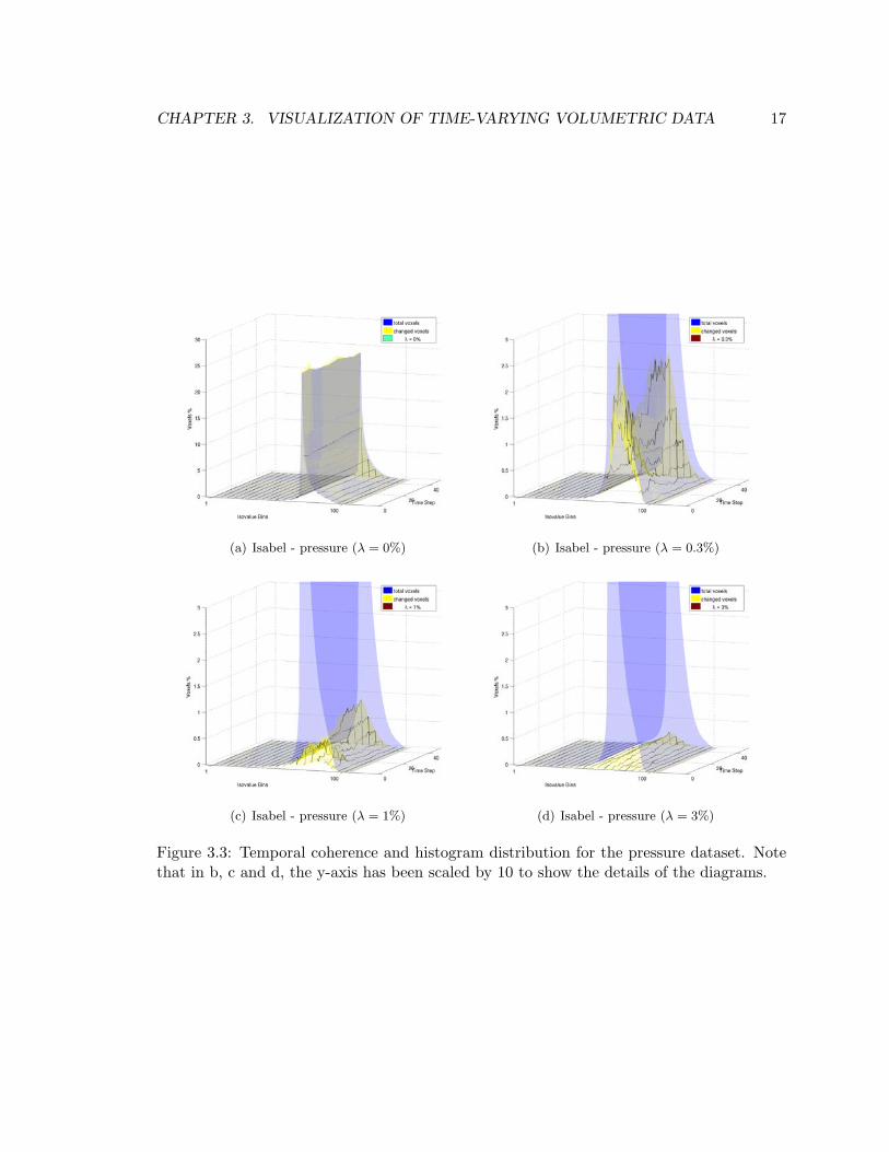
3.3 Temporal coherence and histogram distribution for the pressure dataset. Note
that in b, c and d, the y-axis has been scaled by 10 to show the details of the
diagrams. . . . . . . . . . . . . . . . . . . . . . . . . . . . . . . . . . . . . . . 17
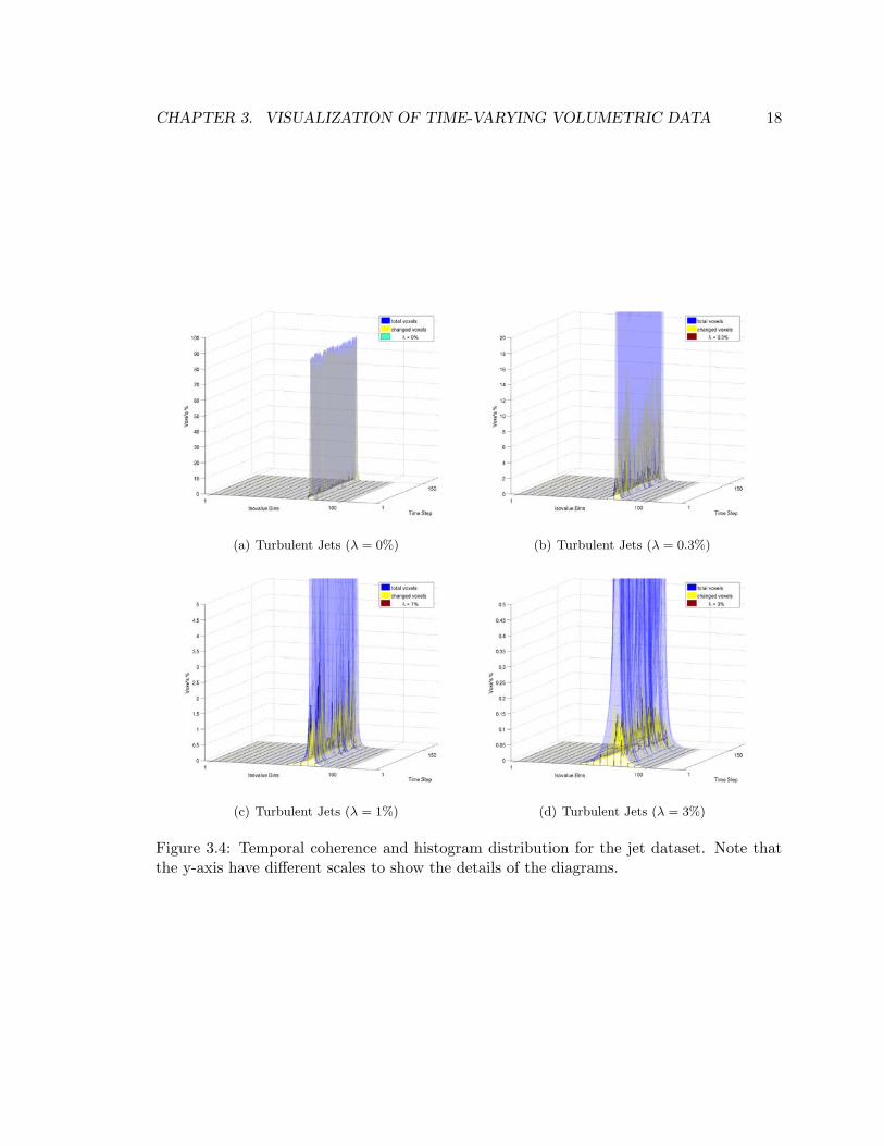
3.4 Temporal coherence and histogram distribution for the jet dataset. Note that
the y-axis have different scales to show the details of the diagrams. . . . . . . 18
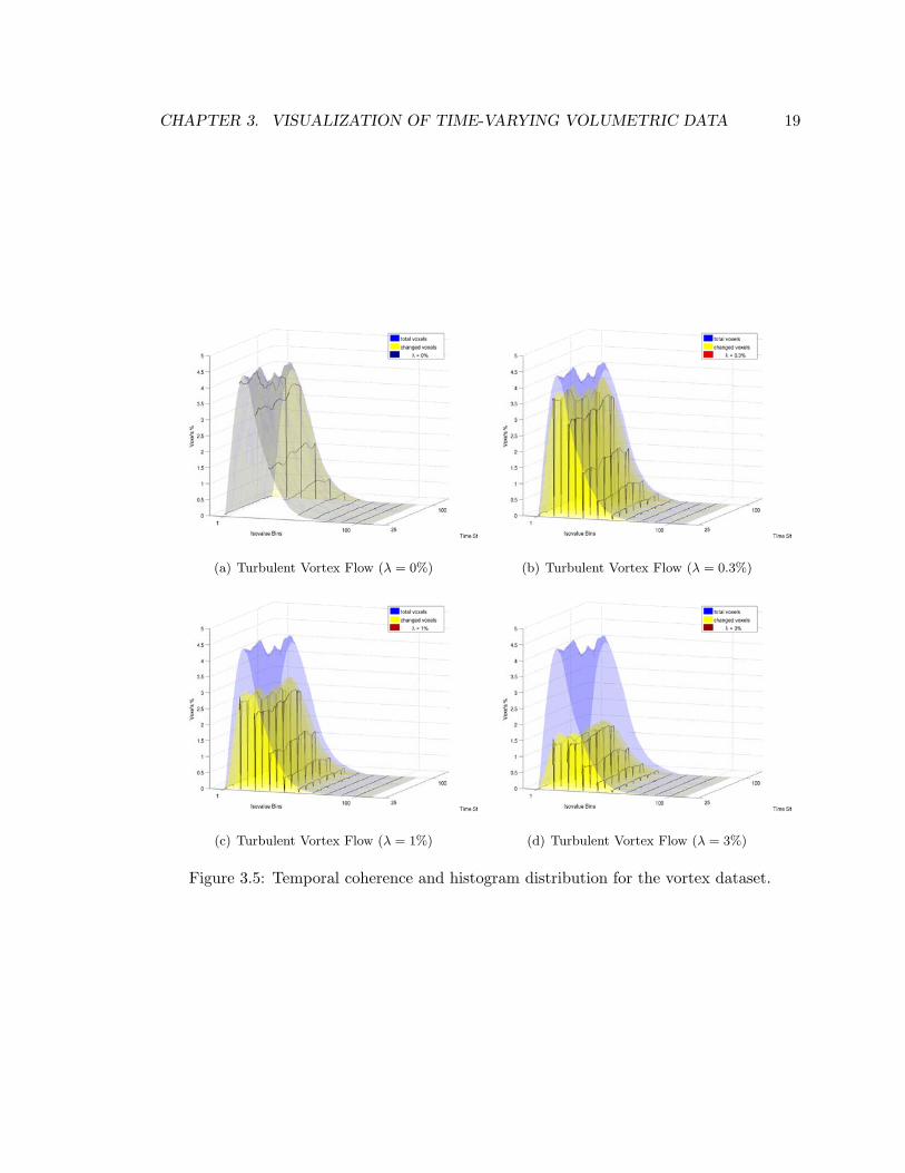
3.5 Temporal coherence and histogram distribution for the vortex dataset. . . . . 19
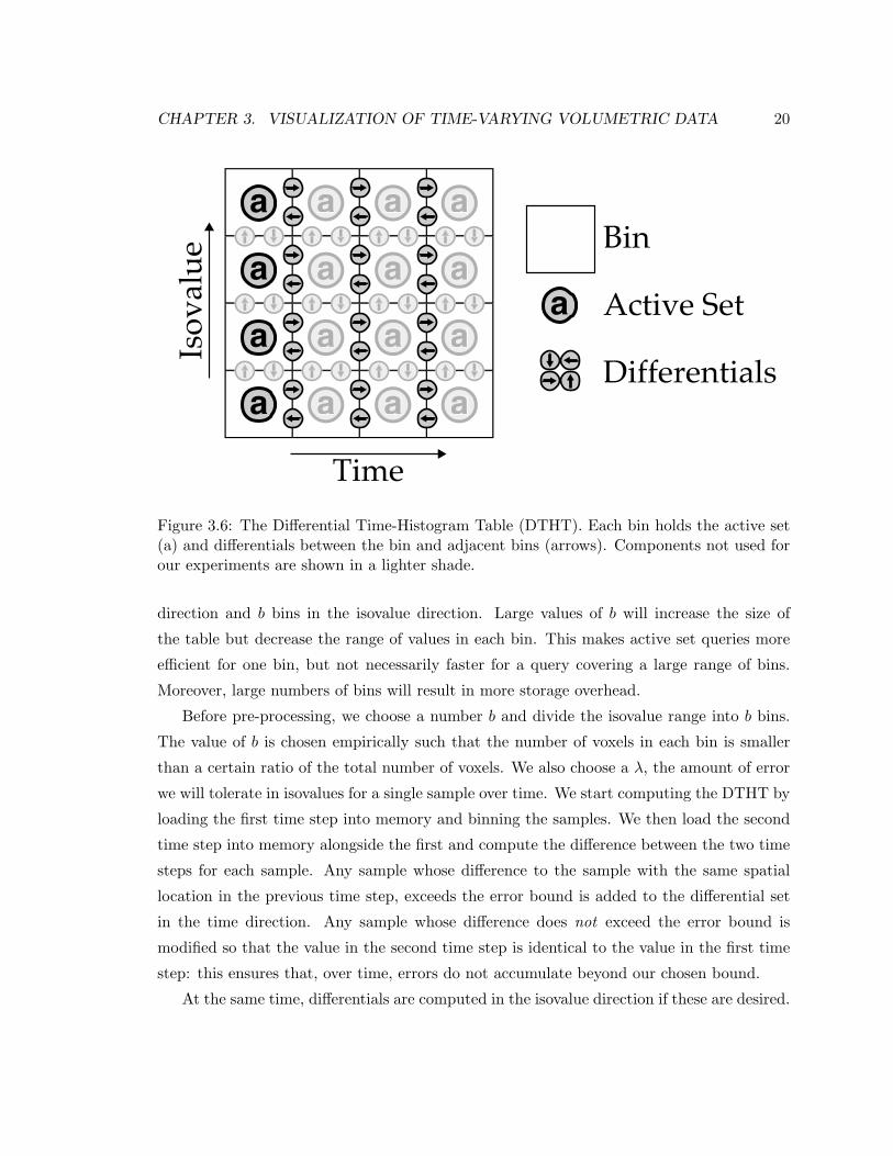
3.6 The Differential Time-Histogram Table (DTHT). Each bin holds the active
set (a) and differentials between the bin and adjacent bins (arrows). Compo-
nents not used for our experiments are shown in a lighter shade. . . . . . . . 20
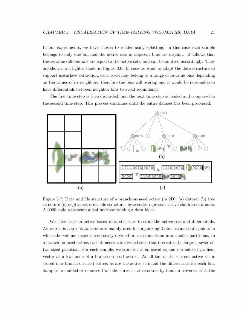
3.7 Data and file structure of a branch-on-need octree (in 2D): (a) dataset (b)
tree structure (c) depth-first order file structure: byte codes represent active
children of a node. A 0000 code represents a leaf node containing a data block. 21
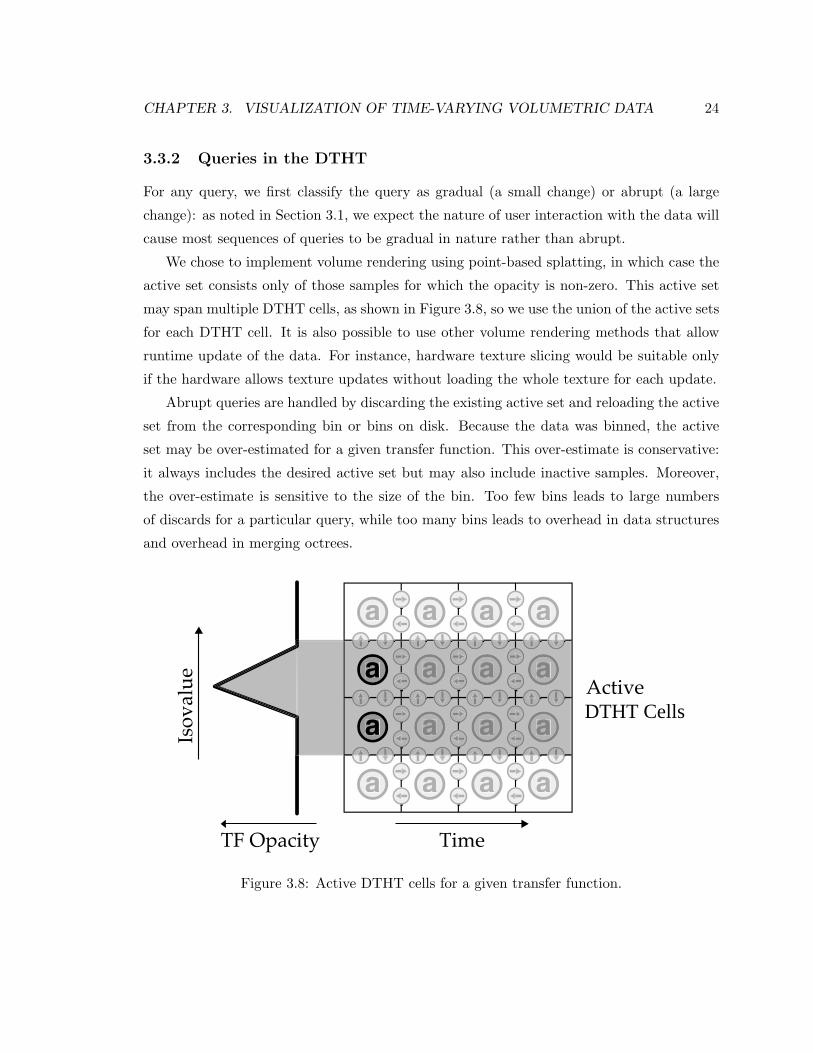
3.8 Active DTHT cells for a given transfer function. . . . . . . . . . . . . . . . . 24
x
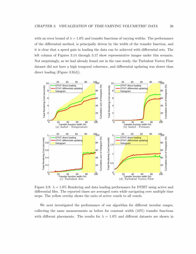
3.9 λ = 1.0% Rendering and data loading performance for DTHT using active
and differential files. The reported times are averaged costs while navigating
over multiple time steps. The yellow overlay shows the ratio of active voxels
to all voxels. . . . . . . . . . . . . . . . . . . . . . . . . . . . . . . . . . . . . . 26
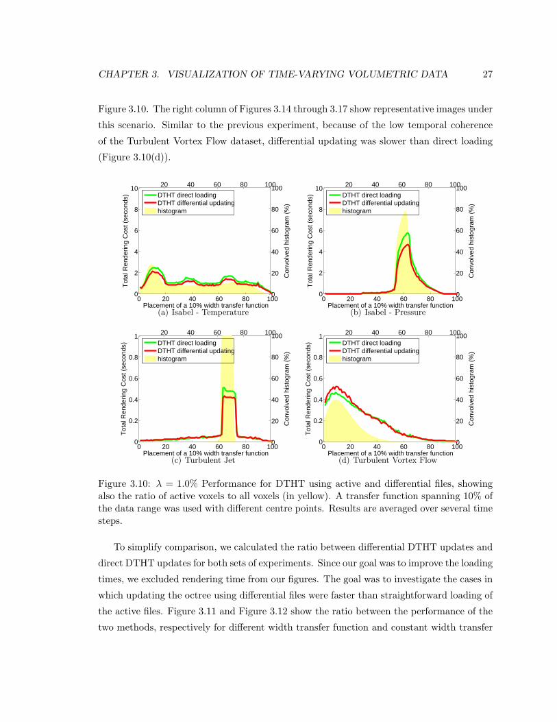
3.10 λ = 1.0% Performance for DTHT using active and differential files, showing
also the ratio of active voxels to all voxels (in yellow). A transfer function
spanning 10% of the data range was used with different centre points. Results
are averaged over several time steps. . . . . . . . . . . . . . . . . . . . . . . . 27
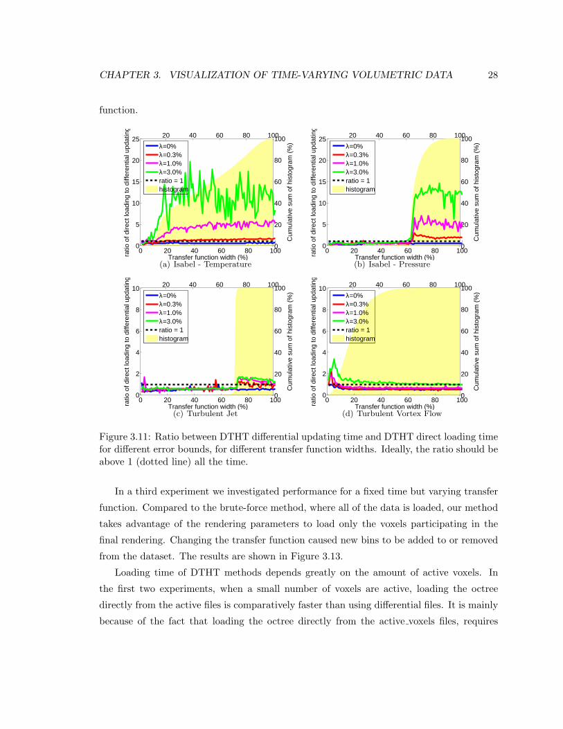
3.11 Ratio between DTHT differential updating time and DTHT direct loading
time for different error bounds, for different transfer function widths. Ideally,
the ratio should be above 1 (dotted line) all the time. . . . . . . . . . . . . . 28
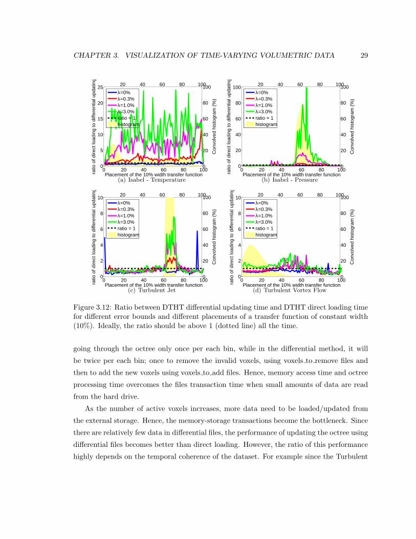
3.12 Ratio between DTHT differential updating time and DTHT direct loading
time for different error bounds and different placements of a transfer function
of constant width (10%). Ideally, the ratio should be above 1 (dotted line)
all the time. . . . . . . . . . . . . . . . . . . . . . . . . . . . . . . . . . . . . . 29
3.13 Loading time of incremental transfer function changes. The graphs show the
time to update the active sets when the active bins are changed in a constant
time step. Increasing the transfer function width (solid-red), only causes
additions to the active set; thus, there is only one peak in the diagram when
a large number of voxels are added to the active set. Changing the placement
of the transfer functions (dotted-blue), requires some voxels to be added and
some voxels to be removed; thus there is one peak in the diagram when a
large number of voxels are added and one peak later when those voxels are
removed. . . . . . . . . . . . . . . . . . . . . . . . . . . . . . . . . . . . . . . . 31
3.14 Rendered images with representative transfer functions for Isabel tempera-
ture dataset. In this figure and the following three figures the left column
shows the results for increasing transfer function width and the right column
shows the results for moving transfer function placement, corresponding to
our experiments in this section. The wired frame shows the octree structure
and the blocks containing active voxels. . . . . . . . . . . . . . . . . . . . . . 32
3.15 Rendered images with representative transfer functions for Isabel pressure
dataset. . . . . . . . . . . . . . . . . . . . . . . . . . . . . . . . . . . . . . . . 33
xi
3.16 Rendered images with representative transfer functions for Turbulent Jets
Flow dataset. . . . . . . . . . . . . . . . . . . . . . . . . . . . . . . . . . . . . 34
3.17 Rendered mages with representative transfer functions for Turbulent Vortex
Flow dataset. . . . . . . . . . . . . . . . . . . . . . . . . . . . . . . . . . . . . 35
4.1 Renderings of the Visible Human Male Head at different levels of details.
Top row: using mean value for approximation. Bottom row: using Gaussian
function for approximation. From left to right, each image represents an
additional level of coarsening by a factor of two in each dimension. . . . . . . 37
4.2 Renderings of a synthetic spherical distance dataset based on the Euclidean
distance to the centre of the volume, at different levels of details. Top row:
using mean value. Bottom row: using Gaussian basis approximation. From
left to right, each image represents an additional level of coarsening by a
factor of two in each dimension. . . . . . . . . . . . . . . . . . . . . . . . . . . 38
4.3 Bottom: a transfer function with the opacities as the vertical axis (V ). Top:
the computed Gaussian basis transfer function; The horizontal and vertical
axes are respectively mean (µ) and standard deviation (σ) and each point
has been drawn with the color and opacity computed for the related µ and σ. 42
4.4 Adding isosurfaces to reveal sharp features in the Richtmyer-Meshkov insta-
bility dataset. Left: splatting. Right: splatting + transparent isosurface. . . . 43
4.5 The structure and indexing of HYBON tree (in 2D). An index of a node
encodes the index of the parent node (2D: index / 4) and the child index of
the node (2D: index % 4) within the parent node. . . . . . . . . . . . . . . . . 46
4.6 Creating cell structures in subvolumes by overlapping border voxels. . . . . . 47
4.7 A high-frequency transfer function (top) and a low-frequency transfer func-
tion (bottom) used for our experiments. . . . . . . . . . . . . . . . . . . . . . 50
xii
4.8 Effects of downsampling distributions with a box low-pass filter on the spher-
ical distance function, rendered using a high-frequency transfer function. Top
most images are highest resolution (643) and quality, bottom images are low-
est resolution (83) and quality. For the high-frequency transfer function cho-
sen, downsampling should blur the thin colored shells into a grey-like color.
The histogram distribution (left), while expensive, does this correctly. The
mean distribution (right) fares poorly, while the Gaussian distribution (mid-
dle) is reasonably effective at low cost. . . . . . . . . . . . . . . . . . . . . . . 53
4.9 Effects of downsampling distributions with a tent low-pass filter on the spher-
ical distance dataset, rendered using a high-frequency transfer function. . . . 54
4.10 Effects of downsampling distributions with a cubic low-pass filter on the
spherical distance dataset, rendered using a high-frequency transfer function. 55
4.11 Effects of downsampling distributions with a box low-pass filter on the Visible
Human Male Head dataset, rendered using a high-frequency transfer function. 56
4.12 Effects of downsampling distributions with a tent low-pass filter on the Visible
Human Male Head dataset, rendered using a high-frequency transfer function. 57
4.13 Effects of downsampling distributions with a cubic low-pass filter on the Vis-
ible Human Male Head dataset, rendered using a high-frequency transfer
function. . . . . . . . . . . . . . . . . . . . . . . . . . . . . . . . . . . . . . . . 58
4.14 Effects of downsampling distributions with a box low-pass filter on the Richtmyer-
Meshkov Instability dataset, rendered using a high-frequency transfer function. 59
4.15 Effects of downsampling distributions with a tent low-pass filter on the Richtmyer-
Meshkov Instability dataset, rendered using a high-frequency transfer function. 60
4.16 Effects of downsampling distributions with a cubic low-pass filter on the
Richtmyer-Meshkov Instability dataset, rendered using a high-frequency trans-
fer function. . . . . . . . . . . . . . . . . . . . . . . . . . . . . . . . . . . . . . 61
4.17 Effects of downsampling distribution with a box low-pass filter on the spheri-
cal distance function , rendered using a low-frequency transfer function. Res-
olution and quality decrease from top to bottom. All three distributions
perform adequately. . . . . . . . . . . . . . . . . . . . . . . . . . . . . . . . . 62
4.18 Effects of downsampling distributions with a tent low-pass filter on the spher-
ical distance dataset, rendered using a low-frequency transfer function. . . . . 63
xiii
4.19 Effects of downsampling distributions with a cubic low-pass filter on the
spherical distance dataset, rendered using a low-frequency transfer function. . 64
4.20 Effects of downsampling distributions with a box low-pass filter on the Visible
Human Male Head dataset, rendered using a low-frequency transfer function. 65
4.21 Effects of downsampling distributions with a tent low-pass filter on the Visible
Human Male Head dataset, rendered using a low-frequency transfer function. 66
4.22 Effects of downsampling distributions with a cubic low-pass filter on the Visi-
ble Human Male Head dataset, rendered using a low-frequency transfer function. 67
4.23 Effects of downsampling distributions with a box low-pass filter on the Richtmyer-
Meshkov Instability dataset, rendered using a low-frequency transfer function. 68
4.24 Effects of downsampling distributions with a tent low-pass filter on the Richtmyer-
Meshkov Instability dataset, rendered using a low-frequency transfer function. 69
4.25 Effects of downsampling distributions with a cubic low-pass filter on the
Richtmyer-Meshkov Instability dataset, rendered using a low-frequency trans-
fer function. . . . . . . . . . . . . . . . . . . . . . . . . . . . . . . . . . . . . . 70
4.26 Errors of the mean and Gaussian approximations of the histogram for the
three test datasets. At a certain level of detail, for each method, the reported
error is the root mean squared error of the voxels’ approximated histogram in
comparison with their actual histogram, for all voxels in that level of coarsening. 71
4.27 Rendering errors of the mean and Gaussian approximations (f) of the his-
togram for the three test datasets using a high-frequency transfer function
(V ). At a certain level of detail, for each method, the reported error is the
root mean squared error of the voxels’ color computed using their approxi-
mated histogram in comparison with their color computed using their actual
histogram, for all voxels in that level of coarsening. . . . . . . . . . . . . . . . 72
4.28 Rendering errors of the mean and Gaussian approximations (f) of the his-
togram for the three test datasets using a medium-frequency transfer function
(V ). At a certain level of detail, for each method, the reported error is the
root mean squared error of the voxels’ color computed using their approxi-
mated histogram in comparison with their color computed using their actual
histogram, for all voxels in that level of coarsening. . . . . . . . . . . . . . . . 73
xiv
Chapter 1
Introduction
“Visualization is concerned with exploring data in such a way as to gain understanding
and insight into the data” [12]. The goal of visualization is “to promote a deeper level of
understanding of the data under investigation and to foster new insight into the underlying
processes, relying on the human’s powerful ability to visualize” [4]. The resulting visual
display of data enables the scientists “to visually perceive features which are hidden in the
data but nevertheless are needed for data exploration and analysis” [40].
One of the research areas in visualization is volume visualization which deals with meth-
ods to explore, analyze and visualize volumetric data acquired in medicine, computational
physics and various other scientific disciplines. In other words, “it is a method of extracting
meaningful information from volumetric data using interactive graphics and imaging and it
is concerned with data representation, modeling, manipulation and rendering” [40].
Volumetric data are acquired by sampling (e.g. CT and MRI), simulation (e.g. com-
putational fluid dynamics) or modeling (voxelization of geometric models) techniques and
are typically represented as a 3D regular or irregular discrete grid of volume elements called
voxels. Voxels are points in 3D, sampled at the grid points and have associated values which
represent some measurable properties or dependent variables (e.g. colour, density, material,
velocity) of the real phenomenon or object residing at the sample location of that voxel.
A Cell consists of a group of neighbor voxels and its geometrical shape depends on the
sampling grid used in sampling the dataset. In a regular Cartesian grid, each group of 8
neighbor voxels on a unit cube’s corners consist a cell.
Over the years many methods have been developed to visualize volumetric data. Among
1
CHAPTER 1. INTRODUCTION 2
those, two broad categories are isosurface extraction and direct volume rendering. Isosur-
face extraction methods approximate surfaces (representing material boundaries contained
within the volumetric data) using geometric primitives, most commonly triangles, and are
usually rendered using conventional graphics accelerator hardware. The resulting surface is
called the isosurface and is defined by a scalar isovalue as a visualization parameter. Some
isosurface extraction methods include marching cubes [32] marching tetrahedra [46], divid-
ing cubes [9] and ray tracing [37]. Representing a surface contained within a volumetric
dataset using geometric primitives can be useful in many applications, particularly when
the datasets contain actual boundaries between materials in the data. However, there are
several drawbacks to this approach. Geometric primitives approximate surfaces contained
within the original data. Adequate approximations may require an excessive number of ge-
ometric primitives and since only a surface representation is used, much of the information
contained within the data is lost during the rendering process [17] (chapter 7).
In response to this, direct volume rendering techniques were developed which create a
2D image directly from 3D volumetric data [26, 54, 23]. Direct volume rendering conveys
more information in a single image than surface rendering, and is thus a valuable tool for
the exploration and analysis of data. Instead of extracting an intermediate representation,
direct volume rendering provides a method for directly rendering the volumetric data by
compositing the original samples onto the image plane. This is typically done using a trans-
fer function which maps the samples to a color and intensity. Direct volume rendering
algorithms include object-order, image-order and domain-based approaches. Object-order
volume rendering approaches such as splatting [54] and shear-warp [23] use a forward map-
ping scheme by decomposing the volume into a set of basic elements and projecting them
individually into an image plane. Image-order algorithms such as raycasting [26], use a back-
ward mapping scheme where rays are cast from each pixel in the image plane through the
volume data to determine the final pixel value. In domain rendering, the spatial 3D data is
first transformed into another domain such as the frequency or the wavelet domain. A pro-
jection is generated using the information of the intermediate domain. Frequency domain
volume rendering [50] is an example of domain rendering algorithms. Due to the increased
computational effort required and the enormous size of volumetric datasets, the ongoing
challenge of research in direct volume rendering is to achieve interactive performance.
Traditional volume visualization methods work well on small and medium-scale datasets.
However, the size of average volumetric data continues to grow as the computational power
CHAPTER 1. INTRODUCTION 3
and scanning resolution increases. Hence, different approaches are required to address the
difficulties associated with the processing of the volumetric data. Large scale volumetric
datasets are commonly characterized as volumetric datasets that exceed the resource limits
of hardware such as memory and computational power. The challenges in visualizing large
datasets are, first, whether the data can be visualized at all and then, whether they can
be processed quickly enough to allow some degree of interactivity (i.e. performance). The
ability to achieve interactive frame rates, in the range of at least a few frames/s, for large
datasets is still an open research challenge. Although various methods have been proposed
to adapt traditional methods to be used with massive parallel hardware [39], it is still a
challenging problem to employ visualization methods on commodity computers.
Major factors that determine the size of a volumetric dataset include dimensionality,
resolution and data modality. Dimensionality is the number of independent coordinates
required to uniquely specify the sample points in the data space. We define resolution
to be the number of samples along each dimension, without considering the actual size of
the sampled phenomenon. Data modality is the number of scalar values per data point.
Considering the first two factors, this thesis addresses two major categories of large-scale
datasets: datasets with many frames of medium resolution volumes (four dimensional) and
datasets with a single high resolution volume. The first category of datasets are called time-
varying volumetric datasets, and are a sequence of varying three dimensional volumetric
data acquired at consecutive time steps. The number of these time steps determines the
resolution along the time dimension. In this thesis we have used time-varying datasets
of sizes ranging from about 128 × 128 × 128 × 150 of 4-byte float samples (1.3 GB) to
500 × 500 × 100 × 50 of 4-byte float samples (4.8 GB).
The second major category is large-scale single frame datasets which have a high res-
olution in the x, y and z dimensions. Since each of the two categories mentioned above
has unique properties and characteristics, we’ve studied these categories separately in this
thesis. The size of the datasets used in this thesis are in the range of about 500×500×2000
1-byte samples (0.5 GB) to 20003 1-byte samples (8 GB).
In this thesis we present new methods to exploit the properties of large-scale volumet-
ric datasets to visualize them efficiently. An overview of algorithms for visualization of
time-varying volumetric datasets and multi-resolution rendering is given in Chapter 2. In
Chapter 3 we study time-varying volumetric datasets and we introduce a new data structure
called Differential Time-Histogram Table [59]. We show how to exploit data characteristics
CHAPTER 1. INTRODUCTION 4
to build a binned data structure to accelerate interactive exploration of such data. Chapter 4
addresses high resolution datasets and introduces a hierarchical data structure to support
multi-resolution data visualization and progressive refinement of visualizations. Extending
the existing techniques, we address the question of multi-resolution rendering quality, using
statistical information to decrease aliasing artifacts in direct volume rendering while using
transparent isosurfaces to decrease the loss of high-frequency features. Finally, Chapter 5
presents the conclusions and discusses directions for future work.
Chapter 2
State of the Art
2.1 State of the Art in Time-Varying Data Visualization
The difficulty of rendering large datasets is well-recognized in the literature, with successive
solutions addressing progressively larger datasets by exploiting various data characteristics.
These characteristics will be thoroughly discussed in Section 3.1. However, in order to
discuss the previous work, we start by defining some of the characteristics briefly in this
chapter. We consider coherence in general as a property of the functions in which small
changes in the functions domain, imply small functional changes. In volumetric datasets,
spatial coherence is coherence of values of voxels with respect to the spatial location. In time-
varying volumetric datasets, temporal coherence is coherence of values of voxels sampled at
different time steps but same spatial location. Histogram distribution determines how well
the values of voxels have been distributed in the overall range of values.
Broadly speaking, the solutions proposed by researchers for visualization of time-varying
datasets have dealt with isosurface extraction and volume rendering as separate topics.
Modern isosurface extraction and volume rendering methods are based on the recognition
that the problem is decomposable into smaller sub-problems [60]. Lorensen & Cline [32]
recognized this and decomposed the extraction of an isosurface over an entire dataset by
extracting the surface for each cell in a cubic mesh independently.
Almost simultaneously, Wyvill, McPheeters & Wyvill [57] exploited spatial coherence
for efficient isosurface extraction in their continuation method. Spatial coherence has also
been exploited for volume rendering [51].
Other researchers [8, 13, 30, 55] exploit spatial distribution for efficient extraction of
5
CHAPTER 2. STATE OF THE ART 6
isosurface active sets. In particular, Wilhelms & van Gelder [55] introduced the Branch-On-
Need Octree (BONO), a space efficient variation of the traditional octree. Octrees, however,
do not always coincide with the spatial distribution of the data, and are not easily applicable
to irregular or unstructured grids.
Livnat et al. [30] introduced the notion of span space - plotting the isovalues spanned
by each cell and building a search structure to find only cells that span a desired isovalue.
Since this represents the range of isovalues in a cell by a single entry in a data structure, it
exploits histogram distribution. Histogram distribution has also been exploited to accelerate
rendering for isosurfaces [6] by computing active set changes with respect to isovalue.
Chiang et al. [7] clustered cells in irregular meshes into meta-cells of roughly equal
numbers of cells, then built an I/O-efficient span space search structure on these meta cells,
again exploiting histogram distribution.
For time-varying data, it is impossible to load an entire dataset plus search structures
into main memory, so researchers have reduced the impact of slow disk access by building
memory-resident search structures and loading data from disk as needed.
Sutton & Hansen [48] extended branch-on-need octrees to time-varying data with Tem-
poral Branch-on-Need Octrees (T-BON), using spatial and temporal coherence to access
only those portions of search structure and data which are necessary to update the active
set.
Similarly, Shen [42] noted that separate span space structures for each time step are inef-
ficient, and proposed a Temporal Hierarchical Index (THI) Tree to suppress search structure
redundancy between time steps, exploiting both histogram distribution and temporal co-
herence.
Reinhard et al. [39] binned samples by isovalue for each time step, loading only those
bins required for a given query: this form of binning exploits histogram distribution but not
temporal coherence.
For volume rendering, Shen & Johnson [45] introduced Differential Volume Rendering,
in which they precomputed the voxels that changed between adjacent time steps, and loaded
only those voxels that changed, principally exploiting temporal coherence.
Shen [43] extended Differential Volume Rendering with Time-Space Partitioning (TSP)
Trees, which exploit both spatial distribution and temporal coherence with an octree repre-
sentation of the volume. Binary trees store spatial and temporal variations for the sub-blocks
CHAPTER 2. STATE OF THE ART 7
of data at the nodes of the tree. This information is used for early termination of a ray-
tracing algorithm, based on a visual error metric. Shen also cached images for each sub-block
in case little or no change occurred between frames. Ma & Shen [34] further extended this
by quantizing the isovalues of the input data and storing them in octrees before computing
differentials.
Finally, Sohn and Bajaj [47] use wavelets to compress time-varying data to a desired
error bound, exploiting temporal coherence as well as spatial and histogram distribution.
In Chapter 3 we discuss statistical characteristics of time-varying datasets and unify
those characteristics in the form of our proposed data structure called Differential Time-
Histogram Table.
2.2 State of the Art in Multi-resolution Techniques
Since it is not always possible to interactively process data in the original sampling resolu-
tion, level of detail and multi-resolution techniques have been proposed by many researchers
to balance between architectural constraints (e.g. performance and memory) and fidelity.
Multi-resolution techniques have been employed in a variety of visual data representation
approaches including geometric rendering [55, 5, 33] and volumetric data visualization [24]
especially for out-of-core applications [43].
Multi-resolution volume rendering techniques principally use spatial hierarchies to rep-
resent different levels of detail. Often the goal is to maintain a specific frame-rate [29] at the
expense of image quality. A partial solution to this is progressive refinement [25, 36, 38], in
which the quality of the rendered image is improved when the user interaction stops.
Shen et al. [43] used image caches attached to the nodes of the octree in order to exploit
temporal coherence for time-varying data. In this thesis we extend that approach and the
idea of frameless rendering [36] in an object order fashion, by re-using previously rendered
images of sub-volumes of the volumetric data in order to avoid re-rendering of those sub-
volumes.
Direct volume rendering techniques [26] use transfer functions (often multi-dimensional [20])
in order to investigate complex scalar data. Surface extraction techniques [32] use geometric
models to represent surface structures in the data. Some approaches [27, 21, 22, 18] combine
both geometric surface models and volumetric transfer functions for hybrid visualization,
improving the insight into a data structure. Often these hybrid methods fail to properly sort
CHAPTER 2. STATE OF THE ART 8
the data during rendering and therefore fail to deal with transparent iso-surfaces combined
with direct volume rendering. In this thesis we deal with this problem and introduce a
framework that allows for accurate hybrid volume rendering. We also demonstrate how to
use transparent iso-surfaces effectively to add high-frequency details at coarse resolutions of
a multi-resolution rendering technique.
Most hierarchical multi-resolution schemes use the mean values of the underlying func-
tion values in order to construct the representations in different levels of detail. Notable
exceptions are wavelet-based multi-resolution schemes [14, 19], which use better filtering
methods to improve the quality of lower levels of the multi-resolution hierarchy. Guthe et
al. [16, 15] use a block based wavelet compression and employ graphics hardware to handle
large datasets at interactive speed.
A couple of the proposed multi-resolution hierarchies for volume rendering address the
underlying transfer function being used during the rendering. Ljung et al. [31] introduce the
use of transfer functions at decompression time to guide a level-of-detail selection scheme.
Wittenbrink et al. [56] have shown that interpolation of the underlying function before
the application of a transfer function is of utmost importance in order to assure the best
quality. Rottger et al. [41] have pointed out that the application of a transfer function to the
underlying scalar data can create arbitrarily high frequencies, making it difficult to render
the data properly. They have proposed Pre-integrated volume rendering to minimize the
impact of the modulation of the underlying signal by the transfer function.
None of these multi-resolution volume rendering methods addresses the proper use of
transfer function and the underlying distribution of the function values to improve the
quality of rendering. In Chapter 4 we propose a novel method to improve the quality of
multi-resolution rendering by approximating the distribution of function values at coarse
levels of detail.
Chapter 3
Visualization of Time-Varying
Volumetric Data
As computing power and scanning precision increase, scientific applications generate time-
varying volumetric data with thousands of time steps and billions of voxels, challenging
our ability to explore and visualize interactively. Although each time step can generally be
rendered efficiently, rendering multiple time steps requires efficient data transfer from disk
storage to main memory to graphics hardware.
We use the temporal coherence of sequential time frames, the spatial distribution of
data values, and the histogram distribution of the data for efficient visualization. Temporal
coherence is used to prevent loading unchanged sample values [48], spatial distribution to
preserve rendering locality between images [55], and histogram distribution to update for
incremental updates during data classification.
Of these, temporal coherence and histogram distribution are encoded in a differential
table computed in a preprocessing step. This differential table is used during visualization to
minimize the amount of data that needs to be loaded from disk between any two successive
images. Spatial distribution is then used to accelerate rendering by retaining unchanged
geometric, topological and combinatorial information between successive images rendered,
based on the differential information loaded from disk.
The major contribution of our method is to identify and analyze statistical characteristics
of large scientific datasets that permit efficient error-bounded visualization. We unify the
statistical properties of the data with the known spatial and temporal coherence of the data
9
CHAPTER 3. VISUALIZATION OF TIME-VARYING VOLUMETRIC DATA 10
in a single differential table used for updating a memory-resident version of the data.
We define coherence and distribution more formally in Section 3.1, and support our
definition of coherence and distribution in Section 3.2 with a case study. In Section 3.3
we show how to exploit data characteristics to build a binned data structure representing
the temporal coherence and spatial and histogram distribution of the data, and how to
use this structure to accelerate interactive exploration of such data. We then present our
implementation results in Section 3.4.
3.1 Data Characteristics
In order to discuss both previous work and our own contributions, we start by defining our
assumed input and the statistical properties of the data that we will exploit for accelerated
visualization: we will support these assertions empirically in our case study in Section 3.2.
Expanding the notation of [8], we define a time-varying dataset as follows: Formally,
a time-varying scalar field is a function f : <4 → <. Such data is often sampled at
fixed locations X = {x1, . . . ,xn} and fixed times T = {t1, . . . , tτ}. Since we exploit this
sampling regularity to accelerate visualization, we assume that our data is of the form
F = {(x, t, f(x, t)) | x ∈ X, t ∈ T}, where each triple (x, t, f(x, t)) is a sample.
Previous researchers report [35] that only a small fraction of F is needed for any given
image generated during visualization. Thus, any image can be thought of as the result of
visualizing a subset of F defined by a query q .
More formally, given F and a condition q (e.g. a transfer function), find the set F|qof all samples (x, t, f(x, t)) for which q is satisfied (e.g. the opacity of f(x, t) is non-zero).
Thus, F|q is the set of samples needed to render q, called the active set of q.
For a query q to extract the isosurface at isovalue h, F|q consists of all samples belonging
to cells whose isovalues span h. In direct volume rendering, the active set has a range of
isovalues for which the opacity transfer function is non-zero.
We now restate our observation: we expect ‖F|q‖ � ‖F‖ where ‖‖ denotes the size of
the set. Moreover, F|q is rarely random, nor is it evenly distributed throughout the dataset.
Instead, F|q tends to consist of large contiguous blocks of samples, due to the continuity
of the physical system underlying the data, and the inherent organization of most physical
systems being studied. We exploit both characteristics to accelerate visualization.
We also exploit the fact that human exploration of data usually involves continuous (i.e.
CHAPTER 3. VISUALIZATION OF TIME-VARYING VOLUMETRIC DATA 11
gradual) variation of queries. Formally, we are interested, not in a single query q , but in a
sequence q1, . . . , qk of closely-related queries, with occasional abrupt changes to a new query
sequence q ′1, . . . , q
′m. We expect that the active sets for any two sequential queries will be
nearly identical, i.e. that F|qi+1 ≈ F|qi.
In particular, we exploit coherence and distribution. Let us denote two samples σ1 =
(x1, t1, f(x1, t1)) and σ2 = (x2, t2, f(x2, t2)), and choose small values δ, λ > 0.
We consider coherence in general as a property of the functions in which small changes
in the functions domain, imply small functional changes.
Spatial coherence is coherence with respect to the spatial dimensions x, y, z of the
domain of f , and is based on the spatial continuity of the physical system. Small spatial
changes imply small functional changes, i.e. if |x1 − x2| < δ and t1 = t2, then |f1 − f2| < λ
for small λ.
Temporal coherence is coherence with respect to the time dimension t of the domain
of f and is based on the temporal continuity of the physical system. Hence, if |t1 − t2| < δ
and x1 = x2, then |f1 − f2| < λ for small λ.
Given two sequential queries qi , qi+1 (e.g. a change in isovalue or time step) which
differ only slightly in space or time, F|qi and F|qi+1 will therefore overlap significantly. We
exploit this to accelerate the task of updating the active set for rendering purposes, focusing
principally on temporal exploration. We also exploit statistical properties of the datasets in
question, which we describe in terms of data distribution:
Histogram distribution is a property of the the range of f and depends largely on
the data being studied and shows how well the function values are distributed over the
functional range. In a well distributed function, the active set for a query is usually a small
subset of the function domain (e.g. only a small number of voxels need to be considered
in order to visualize a particular isosurface). We expect f to be fairly well distributed,
although sampling may affect this.
Spatial distribution is a large scale form of spatial coherence, and is based (again)
on the physical phenomena scientists and engineers study. Although data is commonly
generated over large domains, it is often true that nothing interesting happens in most of
the domain. As a result, the active sets for queries made by the user are often clustered in
a subset of the space.
Histogram distribution is crucial where two sequential queries qi and qi+1 differ only
slightly in the functional dimension. For well-distributed data values, we expect F|qi and
CHAPTER 3. VISUALIZATION OF TIME-VARYING VOLUMETRIC DATA 12
F|qi+1 to be substantially identical: i.e. we can change transfer functions more rapidly by
loading only the new data values required. Moreover, the spatial distribution of the data
allows us to have spatially sparse data structures.
3.2 Case Studies: Data Characteristics of Isabel & Turbu-
lence
As noted in the previous sections, our approach to accelerating visualization depends on
mathematical, statistical and physical properties of the data being studied. Before pro-
gressing further, it is therefore necessary to demonstrate that these properties exist. We do
so by means of case studies of three different datasets.
The first and largest dataset is the Hurricane Isabel dataset provided by the National
Center for Atmospheric Research (NCAR) for the IEEE Visualization Contest 2004. This
dataset has 48 time steps of dimension 500 × 500 × 100, and contains 13 different floating
point scalar variables of which we study the temperature and pressure because they were
different kind of properties by nature and hence were expected to be almost independent
and not to have very similar properties. We have also studied the Turbulent Jets (jets) and
Turbulent Vortex Flow (vortex) datasets provided by D. Silver at Rutgers University and
R. Wilson at University of Iowa to Kwan-Liu Ma at University of California, Davis. The
jets dataset contains 150 time steps of 104× 129× 129 floats, while the vortex dataset were
originally containing 100 time steps of 1283 floating point scalars. Since frame 24 of this
dataset was corrupted, we were only able to use frames 25 through 100.
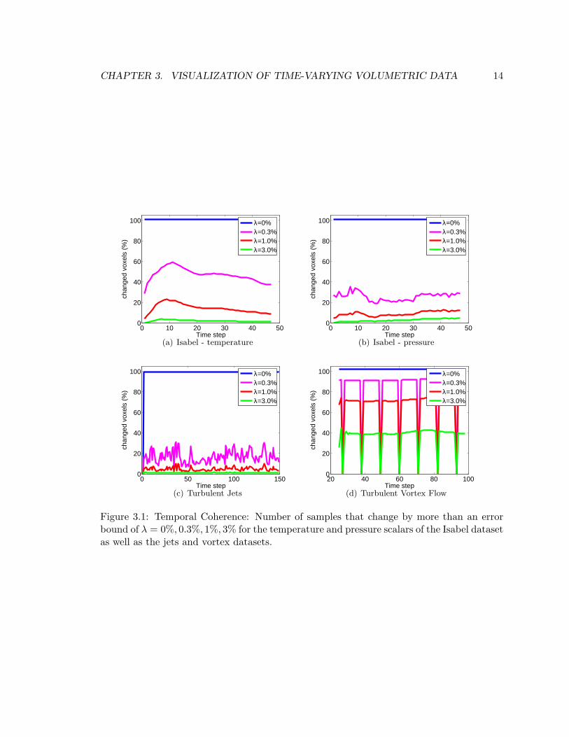
3.2.1 Temporal Coherence
We demonstrate temporal coherence by computing the difference between adjacent time
steps, and graphing the percentage of differences that exceed an error bound. The error
bound (λ%) is expressed as a percentage of the overall data range and its scalar value is
calculated as (max−min)× (λ%). As we see in Figure 3.1, at an error bound of 0%, (where
only identical values are ignored) all of the voxels differ from one time step to the next.
This may be due to numerical inaccuracies in the floating point data. It therefore follows
that 100% of the samples will need to be replaced for the memory-resident version of the
data to be numerically accurate.
CHAPTER 3. VISUALIZATION OF TIME-VARYING VOLUMETRIC DATA 13
However, as we see from the λ = 0.3% plot on the graph, between 40% and 60% of the
samples differ by more than 0.3%. Thus, for a 0.3% error in the isovalues displayed, we can
save as much as 60% of the load time between queries that only change the time step. As
the error bound is increased further, the number of samples to be loaded decreases further:
at 1% error, between 80% and 90% of the samples need not be reloaded, while at 3% error,
over 95% of the samples need not be reloaded.
Similar effects can be seen for pressure in Isabel (Figure 3.1(b)) and for the jets and
vortex datasets (Figure 3.1(c) & (d)). In Figure 3.1(d), we believe that the sharp periodic
dips indicate that certain time steps were inadvertently duplicated. This aside, the overall
conclusion is that relatively small error bounds permit us to avoid loading large numbers of
samples as time changes.
3.2.2 Histogram Distribution
In the last section, we saw that the statistics of temporal coherence give us the opportunity
for efficient differential updates of an active set for a given error bound. It is natural to
ask whether similar statistics are true for small changes in isovalues defining a query. We
show in Figure 3.2 to Figure 3.5 that this is true by examining the histogram distribution
for each dataset.
For these experiments, we set our error bound to 0%, 0.3%, 1% and 3% and computed
the size of the active set for individual data ranges (bins) and for different times. We also
computed the number of samples whose scalar values changed more than the error bound
from the previous time step. For example, we see in Figure 3.2 that temperature isosurfaces
in the Isabel dataset have active sets of less than 5% of the size of a single frame, and that
typically less than half of the samples in those active sets require replacement between one
time step and the next. For pressure (Figure 3.3), although nearly 25% of the samples are
in the active set in the worst case, these samples change little between timesteps, indicating
that the physical phenomenon marked by this pressure feature does not move much in space
between time steps.
In the jets dataset (Figure 3.4), the worst-case behavior is exhibited near the 75th
isovalue bin, where nearly 80% of the samples are in the active set. Although this has
implications for rendering, this set changes little with respect to time. However, in this
dataset these data values constitute most of the “air” surrounding the flow under study and
are likely to be ignored during data exploration because they are usually not interesting for
CHAPTER 3. VISUALIZATION OF TIME-VARYING VOLUMETRIC DATA 14
0 10 20 30 40 500
20
40
60
80
100
Time step
chan
ged
voxe
ls (
%)
λ=0%λ=0.3%λ=1.0%λ=3.0%
(a) Isabel - temperature
0 10 20 30 40 500
20
40
60
80
100
Time step
chan
ged
voxe
ls (
%)
λ=0%λ=0.3%λ=1.0%λ=3.0%
(b) Isabel - pressure
0 50 100 1500
20
40
60
80
100
Time step
chan
ged
voxe
ls (
%)
λ=0%λ=0.3%λ=1.0%λ=3.0%
(c) Turbulent Jets
20 40 60 80 1000
20
40
60
80
100
Time step
chan
ged
voxe
ls (
%)
λ=0%λ=0.3%λ=1.0%λ=3.0%
(d) Turbulent Vortex Flow
Figure 3.1: Temporal Coherence: Number of samples that change by more than an errorbound of λ = 0%, 0.3%, 1%, 3% for the temperature and pressure scalars of the Isabel datasetas well as the jets and vortex datasets.
CHAPTER 3. VISUALIZATION OF TIME-VARYING VOLUMETRIC DATA 15
the scientists.
In the vortex dataset (Figure 3.5), we see again that data bins involve relatively few
samples, and that these samples have some degree of temporal coherence.
In general, our studies show that although we can’t expect all datasets to have a fairly
well distributed histogram, the temporal coherence gives us the opportunity to reduce the
updates of active sets during the changing of time steps.
3.2.3 Spatial Distribution
Unlike histogram distribution, spatial distribution is harder to test, as it is best measured in
terms of the spatial data structure used to store the data. We therefore defer consideration
of spatial distribution to the discussion of Table 3.1 in Section 3.3.
3.3 Differential Time-Histogram Table
In the previous section, we demonstrated that temporal coherence and histogram distri-
bution offer the opportunity to reduce load times for gradual variations of visualization
queries when visualizing large time-varying datasets. To achieve the hypothesized reduction
in load-time we introduce a new data structure called the Differential Time-Histogram Table
(DTHT) along with an efficient algorithm for performing regular and differential queries in
order to visualize the dataset.
To exploit temporal coherence and histogram distribution, we apply differential visual-
ization in the temporal direction and binning in the isovalue direction. Since we expect user
exploration of the data to consist mostly of gradual variations in queries, we precompute the
differences between successive queries and store them as differentials. We modify temporal
coherence by including in the differential set only those samples for which the error exceeds
a chosen bound, further reducing the number of samples to be loaded at each time step.
3.3.1 Computing the DTHT
Our DTHT, shown in Figure 3.6, stores samples in a two-dimensional table of bins defined
by the isovalue range and the time step. In each bin, we store the active set (a), and a set
of differences (arrows) between the active sets of adjacent bins.
For a given dataset with τ time steps, we create a DTHT with τ bins in the temporal
CHAPTER 3. VISUALIZATION OF TIME-VARYING VOLUMETRIC DATA 16
(a) Isabel - temperature (λ = 0%) (b) Isabel - temperature (λ = 0.3%)
(c) Isabel - temperature (λ = 1%) (d) Isabel - temperature (λ = 3%)
Figure 3.2: Temporal coherence and histogram distribution for the temperature dataset: Inthis figure and following three figures, the striped yellow plot shows the number of samplesthat change by more than the error bound λ. The blue plot represents the number of samplesper bin (histogram), at each time step. The isovalue range is divided into 100 isovalue bins.
CHAPTER 3. VISUALIZATION OF TIME-VARYING VOLUMETRIC DATA 17
(a) Isabel - pressure (λ = 0%) (b) Isabel - pressure (λ = 0.3%)
(c) Isabel - pressure (λ = 1%) (d) Isabel - pressure (λ = 3%)
Figure 3.3: Temporal coherence and histogram distribution for the pressure dataset. Notethat in b, c and d, the y-axis has been scaled by 10 to show the details of the diagrams.
CHAPTER 3. VISUALIZATION OF TIME-VARYING VOLUMETRIC DATA 18
(a) Turbulent Jets (λ = 0%) (b) Turbulent Jets (λ = 0.3%)
(c) Turbulent Jets (λ = 1%) (d) Turbulent Jets (λ = 3%)
Figure 3.4: Temporal coherence and histogram distribution for the jet dataset. Note thatthe y-axis have different scales to show the details of the diagrams.
CHAPTER 3. VISUALIZATION OF TIME-VARYING VOLUMETRIC DATA 19
(a) Turbulent Vortex Flow (λ = 0%) (b) Turbulent Vortex Flow (λ = 0.3%)
(c) Turbulent Vortex Flow (λ = 1%) (d) Turbulent Vortex Flow (λ = 3%)
Figure 3.5: Temporal coherence and histogram distribution for the vortex dataset.
CHAPTER 3. VISUALIZATION OF TIME-VARYING VOLUMETRIC DATA 20
aaaa
aaaa
aaaa
aaaa
a
Bin
Active Set
Differentials
Time
Iso
va
lue
Figure 3.6: The Differential Time-Histogram Table (DTHT). Each bin holds the active set(a) and differentials between the bin and adjacent bins (arrows). Components not used forour experiments are shown in a lighter shade.
direction and b bins in the isovalue direction. Large values of b will increase the size of
the table but decrease the range of values in each bin. This makes active set queries more
efficient for one bin, but not necessarily faster for a query covering a large range of bins.
Moreover, large numbers of bins will result in more storage overhead.
Before pre-processing, we choose a number b and divide the isovalue range into b bins.
The value of b is chosen empirically such that the number of voxels in each bin is smaller
than a certain ratio of the total number of voxels. We also choose a λ, the amount of error
we will tolerate in isovalues for a single sample over time. We start computing the DTHT by
loading the first time step into memory and binning the samples. We then load the second
time step into memory alongside the first and compute the difference between the two time
steps for each sample. Any sample whose difference to the sample with the same spatial
location in the previous time step, exceeds the error bound is added to the differential set
in the time direction. Any sample whose difference does not exceed the error bound is
modified so that the value in the second time step is identical to the value in the first time
step: this ensures that, over time, errors do not accumulate beyond our chosen bound.
At the same time, differentials are computed in the isovalue direction if these are desired.
CHAPTER 3. VISUALIZATION OF TIME-VARYING VOLUMETRIC DATA 21
In our experiments, we have chosen to render using splatting: in this case each sample
belongs to only one bin and the active sets in adjacent bins are disjoint. It follows that
the isovalue differentials are equal to the active sets, and can be omitted accordingly. They
are shown in a lighter shade in Figure 3.6. In case we want to adapt the data structure to
support isosurface extraction, each voxel may belong to a range of isovalue bins depending
on the values of its neighbors; therefore the bins will overlap and it would be reasonable to
have differentials between neighbor bins to avoid redundancy.
The first time step is then discarded, and the next time step is loaded and compared to
the second time step. This process continues until the entire dataset has been processed.
(a)
(b)
(c)
1011 0010 0000 1110 0000 0000
00000000 1100 0000
1011
0010 1110 1100
Figure 3.7: Data and file structure of a branch-on-need octree (in 2D): (a) dataset (b) treestructure (c) depth-first order file structure: byte codes represent active children of a node.A 0000 code represents a leaf node containing a data block.
We have used an octree based data structure to store the active sets and differentials.
An octree is a tree data structure mainly used for organizing 3-dimensional data points in
which the volume space is recursively divided in each dimension into smaller partitions. In
a branch-on-need octree, each dimension is divided such that it creates the largest power-of-
two sized partition. For each sample, we store location, isovalue, and normalized gradient
vector at a leaf node of a branch-on-need octree. At all times, the current active set is
stored in a branch-on-need octree, as are the active sets and the differentials for each bin.
Samples are added or removed from the current active octree by tandem traversal with the
CHAPTER 3. VISUALIZATION OF TIME-VARYING VOLUMETRIC DATA 22
differential octrees of the active bins. Figure 3.7 shows the octree and its file structure.
Figure 3.7(a) demonstrates a sample dataset and the space division in 2D. Figure 3.7(b)
shows the tree data structure and Figure 3.7(c) shows the corresponding file structure to
store the tree. The tree is stored and loaded in a depth first order. Starting from the root
node, a byte-code is stored to indicate non-empty children nodes. Then for the leaf nodes
the data block is stored. Otherwise the non-empty sub-trees are processed recursively.
Instead of single samples, however, we store entire blocks of data (typically 32×32×32)
at octree leaves, either in linked lists or fixed size arrays. We use linked lists if no more than
60% of the block is active, in which we store the spatial locations of the samples as well as
their values. However, if more than 60% is active, we use a fixed size array where the spatial
locations of the samples are implied from their index in the array. The threshold of 60% is
computed to be the point at which the overhead of including spatial positions (indices) of
samples in a linked list is almost equal to the overhead of keeping empty samples in an array.
We save space by storing sample locations relative to the octree cell instead of absolutely,
requiring fewer bits of precision.
Moreover, octrees are memory coherent, so updates are more efficient than linear lists,
although at the expense of a larger memory footprint, as shown in Table 3.1. We note,
however, that the memory footprint is principally determined by the size of the octrees for
the active sets.
Further reductions in storage are possible depending on the nature of the queries to
be executed. We assume that abrupt queries are few and far between, and dispense with
storing active sets explicitly except for the first time step. If an abrupt query is made at
time t, we can construct the active set by starting with the corresponding active set at time
0 and applying all differential sets up to time t. Doing so reduces the amount of storage
required, as shown in the third column of Table 3.1. As with the isovalue differentials, we
indicate this in Figure 3.6 by displaying the unused active sets in a lighter shade. We can
also store active sets in a subset of a priorly chosen key frames so that we always start from
the nearest keyframe instead of starting from the first frame. Another way of reducing the
storage is to remove the active sets and differentials for the non-interesting isovalue ranges.
For example we can identify and remove the bins that contain the values of empty spaces
surrounding the actual phenomena of interest. This can have a huge impact depending on
the nature of the dataset, e.g. for the Turbulent Jets dataset, we can remove up to 80% of
the overall data.
CHAPTER 3. VISUALIZATION OF TIME-VARYING VOLUMETRIC DATA 23
Structure List Octree Octree
All Active Sets 1st Active Set
λ GB %age GB %age GB %ageIsabel - temperature
0.0% 34.6 737% 27.7 591% 18.5 394%0.3% 22.4 477% 17.9 382% 8.7 186%1.0% 15.0 320% 12.0 256% 2.8 60%3.0% 12.2 260% 9.8 209% 0.59 12%Isabel - pressure
0.0% 34.6 737% 27.7 590% 18.5 394%0.3% 17.6 371% 14.1 301% 4.9 104%1.0% 13.8 294% 11.1 237% 1.9 40%3.0% 12.4 264% 9.9 211% 0.72 15%Turbulent Jets
0.0% 7.4 673% 5.0 455% 3.4 330%0.3% 3.4 310% 2.4 216% 0.71 70%1.0% 2.8 255% 1.9 173% 0.20 20%3.0% 2.6 236% 1.8 164% 0.06 6%Turbulent Vortex Flow
0.0% 4.6 731% 3.7 588% 2.5 394%0.3% 4.0 636% 3.2 509% 2.0 320%1.0% 3.5 556% 2.8 445% 1.6 252%3.0% 2.6 413% 2.1 334% 0.93 150%
Table 3.1: Size (in GB and percent of original dataset) of DTHT using lists and octrees withall or only the first active set stored. Storing all active sets is expensive storage-wise, butit enables us to access any time step directly. As an alternative we can store only the firstactive set and use differentials to obtain the active sets in other time steps. This improvesthe storage requirement substantially but does not allow direct access to time steps.
CHAPTER 3. VISUALIZATION OF TIME-VARYING VOLUMETRIC DATA 24
3.3.2 Queries in the DTHT
For any query, we first classify the query as gradual (a small change) or abrupt (a large
change): as noted in Section 3.1, we expect the nature of user interaction with the data will
cause most sequences of queries to be gradual in nature rather than abrupt.
We chose to implement volume rendering using point-based splatting, in which case the
active set consists only of those samples for which the opacity is non-zero. This active set
may span multiple DTHT cells, as shown in Figure 3.8, so we use the union of the active sets
for each DTHT cell. It is also possible to use other volume rendering methods that allow
runtime update of the data. For instance, hardware texture slicing would be suitable only
if the hardware allows texture updates without loading the whole texture for each update.
Abrupt queries are handled by discarding the existing active set and reloading the active
set from the corresponding bin or bins on disk. Because the data was binned, the active
set may be over-estimated for a given transfer function. This over-estimate is conservative:
it always includes the desired active set but may also include inactive samples. Moreover,
the over-estimate is sensitive to the size of the bin. Too few bins leads to large numbers
of discards for a particular query, while too many bins leads to overhead in data structures
and overhead in merging octrees.
aaaa
aaaa
Time
Iso
val
ue
TF Opacity
aaaa
aaaaActiveDTHT Cells
Figure 3.8: Active DTHT cells for a given transfer function.
CHAPTER 3. VISUALIZATION OF TIME-VARYING VOLUMETRIC DATA 25
Gradual queries in the temporal direction edit the active set using differentials for each
bin spanned by the transfer function. Since forward and backward differentials are reciprocal
in nature, for each arrow we only store the set of samples that needs to be added in that
direction. The set of samples that needs to be removed is then the set of samples to be
added on the reciprocal arrow between the same bins.
Gradual queries in the isovalue direction discard all samples in a bin when the transfer
function no longer spans that bin, and add all samples in a bin when the transfer function
first spans that bin. It should be noted that random access to voxels in our octree based
data structure will not be efficient since it requires top down traversing of all octrees to
access a voxel. Hence, visualizing multi-modal data would be generally difficult in the cases
where different measures are stored in separate structures. For example it would be hard
to visualize an isosurface of temperature from one structure and color it with the value of
pressure from another structure.
Similar to TSP tree [43], for faster rendering, partial images for each base level block in
the current active octree are stored as image caches, and are used when the blocks don’t
change. Since we update base level blocks in the octree only when changes exceed the
λ-bound, these partial images can survive a few time steps.
3.4 Results and Discussion
We implemented our Differential Time-Histogram Table algorithm and visualized different
scalar time-varying datasets introduced in Section 3.2, using a 3.06 GHz Intel Xeon proces-
sor, 2 GB of main memory and an nVidia AGP 8x GeForce 6800 graphics card, with data
stored on a fileserver on a 100 Mb/s Local Area Network.
In our experiments we used b = 100 isovalue bins, set the base-level brick size in the
octrees to 32 × 32 × 32, and tested four different values for error bounds (λ = 0%, 0.3%,
1.0%, 3.0%).
In our first experiment we controlled the number of active voxels by changing the width
of a left-aligned transfer function to gradually increase the range of isovalues that are set
to non-transparent opacity values. Starting with a 0% width transfer function covering no
bins, we increased the width until all data values were classified as non-transparent and all
bins were loaded. In Figure 3.9, we compared the performance of DTHT active sets alone,
with the performance of DTHT using active and differential sets, rendering each dataset
CHAPTER 3. VISUALIZATION OF TIME-VARYING VOLUMETRIC DATA 26
with an error bound of λ = 1.0% and transfer functions of varying widths. The performance
of the differential method, is principally driven by the width of the transfer function, and
it is clear that a speed gain in loading the data can be achieved with differential sets. The
left column of Figures 3.14 through 3.17 show representative images under this scenario.
Not surprisingly, as we had already found out in the case study, the Turbulent Vortex Flow
dataset did not have a high temporal coherence, and differential updating was slower than
direct loading (Figure 3.9(d)).
20 40 60 80 100
0
20
40
60
80
100
Cum
ulat
ive
sum
of h
isto
gram
(%
)
0 20 40 60 80 1000
2
4
6
8
10
Transfer function width (%)
Tot
al R
ende
ring
Cos
t (se
cond
s) DTHT direct loadingDTHT differential updatinghistogram
(a) Isabel - Temperature
20 40 60 80 100
0
20
40
60
80
100
Cum
ulat
ive
sum
of h
isto
gram
(%
)
0 20 40 60 80 1000
2
4
6
8
10
Transfer function width (%)
Tot
al R
ende
ring
Cos
t (se
cond
s) DTHT direct loadingDTHT differential updatinghistogram
(b) Isabel - Pressure
20 40 60 80 100
0
20
40
60
80
100
Cum
ulat
ive
sum
of h
isto
gram
(%
)
0 20 40 60 80 1000
0.2
0.4
0.6
0.8
1
Transfer function width (%)
Tot
al R
ende
ring
Cos
t (se
cond
s) DTHT direct loadingDTHT differential updatinghistogram
(c) Turbulent Jets
20 40 60 80 100
0
20
40
60
80
100
Cum
ulat
ive
sum
of h
isto
gram
(%
)
0 20 40 60 80 1000
0.5
1
1.5
2
Transfer function width (%)
Tot
al R
ende
ring
Cos
t (se
cond
s) DTHT direct loadingDTHT differential updatinghistogram
(d) Turbulent Vortex Flow
Figure 3.9: λ = 1.0% Rendering and data loading performance for DTHT using active anddifferential files. The reported times are averaged costs while navigating over multiple timesteps. The yellow overlay shows the ratio of active voxels to all voxels.
We next investigated the performance of our algorithm for different isovalue ranges,
collecting the same measurements as before for constant width (10%) transfer functions
with different placements. The results for λ = 1.0% and different datasets are shown in
CHAPTER 3. VISUALIZATION OF TIME-VARYING VOLUMETRIC DATA 27
Figure 3.10. The right column of Figures 3.14 through 3.17 show representative images under
this scenario. Similar to the previous experiment, because of the low temporal coherence
of the Turbulent Vortex Flow dataset, differential updating was slower than direct loading
(Figure 3.10(d)).
20 40 60 80 100
0
20
40
60
80
100
Con
volv
ed h
isto
gram
(%
)
0 20 40 60 80 1000
2
4
6
8
10
Placement of a 10% width transfer function
Tot
al R
ende
ring
Cos
t (se
cond
s) DTHT direct loadingDTHT differential updatinghistogram
(a) Isabel - Temperature
20 40 60 80 100
0
20
40
60
80
100
Con
volv
ed h
isto
gram
(%
)
0 20 40 60 80 1000
2
4
6
8
10
Placement of a 10% width transfer functionT
otal
Ren
derin
g C
ost (
seco
nds) DTHT direct loading
DTHT differential updatinghistogram
(b) Isabel - Pressure
20 40 60 80 100
0
20
40
60
80
100
Con
volv
ed h
isto
gram
(%
)
0 20 40 60 80 1000
0.2
0.4
0.6
0.8
1
Placement of a 10% width transfer function
Tot
al R
ende
ring
Cos
t (se
cond
s) DTHT direct loadingDTHT differential updatinghistogram
(c) Turbulent Jet
20 40 60 80 100
0
20
40
60
80
100
Con
volv
ed h
isto
gram
(%
)
0 20 40 60 80 1000
0.2
0.4
0.6
0.8
1
Placement of a 10% width transfer function
Tot
al R
ende
ring
Cos
t (se
cond
s) DTHT direct loadingDTHT differential updatinghistogram
(d) Turbulent Vortex Flow
Figure 3.10: λ = 1.0% Performance for DTHT using active and differential files, showingalso the ratio of active voxels to all voxels (in yellow). A transfer function spanning 10% ofthe data range was used with different centre points. Results are averaged over several timesteps.
To simplify comparison, we calculated the ratio between differential DTHT updates and
direct DTHT updates for both sets of experiments. Since our goal was to improve the loading
times, we excluded rendering time from our figures. The goal was to investigate the cases in
which updating the octree using differential files were faster than straightforward loading of
the active files. Figure 3.11 and Figure 3.12 show the ratio between the performance of the
two methods, respectively for different width transfer function and constant width transfer
CHAPTER 3. VISUALIZATION OF TIME-VARYING VOLUMETRIC DATA 28
function.
20 40 60 80 100
0
20
40
60
80
100
Cum
ulat
ive
sum
of h
isto
gram
(%
)
0 20 40 60 80 1000
5
10
15
20
25
Transfer function width (%)ratio
of d
irect
load
ing
to d
iffer
entia
l upd
atin
g
λ=0%λ=0.3%λ=1.0%λ=3.0%ratio = 1histogram
(a) Isabel - Temperature
20 40 60 80 100
0
20
40
60
80
100
Cum
ulat
ive
sum
of h
isto
gram
(%
)
0 20 40 60 80 1000
5
10
15
20
25
Transfer function width (%)ratio
of d
irect
load
ing
to d
iffer
entia
l upd
atin
g
λ=0%λ=0.3%λ=1.0%λ=3.0%ratio = 1histogram
(b) Isabel - Pressure
20 40 60 80 100
0
20
40
60
80
100C
umul
ativ
e su
m o
f his
togr
am (
%)
0 20 40 60 80 1000
2
4
6
8
10
Transfer function width (%)ratio
of d
irect
load
ing
to d
iffer
entia
l upd
atin
g
λ=0%λ=0.3%λ=1.0%λ=3.0%ratio = 1histogram
(c) Turbulent Jet
20 40 60 80 100
0
20
40
60
80
100
Cum
ulat
ive
sum
of h
isto
gram
(%
)
0 20 40 60 80 1000
2
4
6
8
10
Transfer function width (%)ratio
of d
irect
load
ing
to d
iffer
entia
l upd
atin
g
λ=0%λ=0.3%λ=1.0%λ=3.0%ratio = 1histogram
(d) Turbulent Vortex Flow
Figure 3.11: Ratio between DTHT differential updating time and DTHT direct loading timefor different error bounds, for different transfer function widths. Ideally, the ratio should beabove 1 (dotted line) all the time.
In a third experiment we investigated performance for a fixed time but varying transfer
function. Compared to the brute-force method, where all of the data is loaded, our method
takes advantage of the rendering parameters to load only the voxels participating in the
final rendering. Changing the transfer function caused new bins to be added to or removed
from the dataset. The results are shown in Figure 3.13.
Loading time of DTHT methods depends greatly on the amount of active voxels. In
the first two experiments, when a small number of voxels are active, loading the octree
directly from the active files is comparatively faster than using differential files. It is mainly
because of the fact that loading the octree directly from the active voxels files, requires
CHAPTER 3. VISUALIZATION OF TIME-VARYING VOLUMETRIC DATA 29
20 40 60 80 100
0
20
40
60
80
100
Con
volv
ed h
isto
gram
(%
)
0 20 40 60 80 1000
5
10
15
20
25
Placement of the 10% width transfer functionratio
of d
irect
load
ing
to d
iffer
entia
l upd
atin
gλ=0%λ=0.3%λ=1.0%λ=3.0%ratio = 1histogram
(a) Isabel - Temperature
20 40 60 80 100
0
20
40
60
80
100
Con
volv
ed h
isto
gram
(%
)
0 20 40 60 80 1000
20
40
60
80
100
Placement of the 10% width transfer functionratio
of d
irect
load
ing
to d
iffer
entia
l upd
atin
g
λ=0%λ=0.3%λ=1.0%λ=3.0%ratio = 1histogram
(b) Isabel - Pressure
20 40 60 80 100
0
20
40
60
80
100
Con
volv
ed h
isto
gram
(%
)
0 20 40 60 80 1000
2
4
6
8
10
Placement of the 10% width transfer functionratio
of d
irect
load
ing
to d
iffer
entia
l upd
atin
g
λ=0%λ=0.3%λ=1.0%λ=3.0%ratio = 1histogram
(c) Turbulent Jet
20 40 60 80 100
0
20
40
60
80
100
Con
volv
ed h
isto
gram
(%
)
0 20 40 60 80 1000
2
4
6
8
10
Placement of the 10% width transfer functionratio
of d
irect
load
ing
to d
iffer
entia
l upd
atin
g
λ=0%λ=0.3%λ=1.0%λ=3.0%ratio = 1histogram
(d) Turbulent Vortex Flow
Figure 3.12: Ratio between DTHT differential updating time and DTHT direct loading timefor different error bounds and different placements of a transfer function of constant width(10%). Ideally, the ratio should be above 1 (dotted line) all the time.
going through the octree only once per each bin, while in the differential method, it will
be twice per each bin; once to remove the invalid voxels, using voxels to remove files and
then to add the new voxels using voxels to add files. Hence, memory access time and octree
processing time overcomes the files transaction time when small amounts of data are read
from the hard drive.
As the number of active voxels increases, more data need to be loaded/updated from
the external storage. Hence, the memory-storage transactions become the bottleneck. Since
there are relatively few data in differential files, the performance of updating the octree using
differential files becomes better than direct loading. However, the ratio of this performance
highly depends on the temporal coherence of the dataset. For example since the Turbulent
CHAPTER 3. VISUALIZATION OF TIME-VARYING VOLUMETRIC DATA 30
Vortex Flow dataset is not as temporally coherent as the other three datasets, even with a
1.0% error bound, differential updating is slower than the direct loading because the number
of voxels to add + voxels to remove is larger than the number of active voxels.
Noise in the diagrams is mainly due to loading the data through a local area network
connection which is fast, but does not always provide a constant data rate. There are also
large variations in some parts of Figure 3.11 and Figure 3.12. It can be seen that most of
the noise is in the parts in which not many voxels are active. This is because of the fact
that as the expected loading times become smaller, the slightest activities in the hardware
or the operating system can result in more relative noise in the measured times.
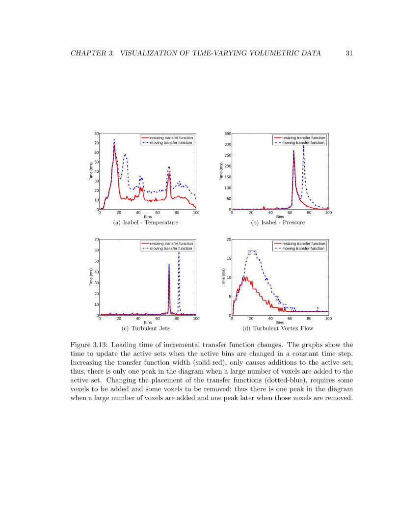
CHAPTER 3. VISUALIZATION OF TIME-VARYING VOLUMETRIC DATA 31
0 20 40 60 80 1000
10
20
30
40
50
60
70
80
Bins
Tim
e (m
s)
resizing transfer functionmoving transfer function
(a) Isabel - Temperature
0 20 40 60 80 1000
50
100
150
200
250
300
350
BinsT
ime
(ms)
resizing transfer functionmoving transfer function
(b) Isabel - Pressure
0 20 40 60 80 1000
10
20
30
40
50
60
70
Bins
Tim
e (m
s)
resizing transfer functionmoving transfer function
(c) Turbulent Jets
0 20 40 60 80 1000
5
10
15
20
Bins
Tim
e (m
s)
resizing transfer functionmoving transfer function
(d) Turbulent Vortex Flow
Figure 3.13: Loading time of incremental transfer function changes. The graphs show thetime to update the active sets when the active bins are changed in a constant time step.Increasing the transfer function width (solid-red), only causes additions to the active set;thus, there is only one peak in the diagram when a large number of voxels are added to theactive set. Changing the placement of the transfer functions (dotted-blue), requires somevoxels to be added and some voxels to be removed; thus there is one peak in the diagramwhen a large number of voxels are added and one peak later when those voxels are removed.
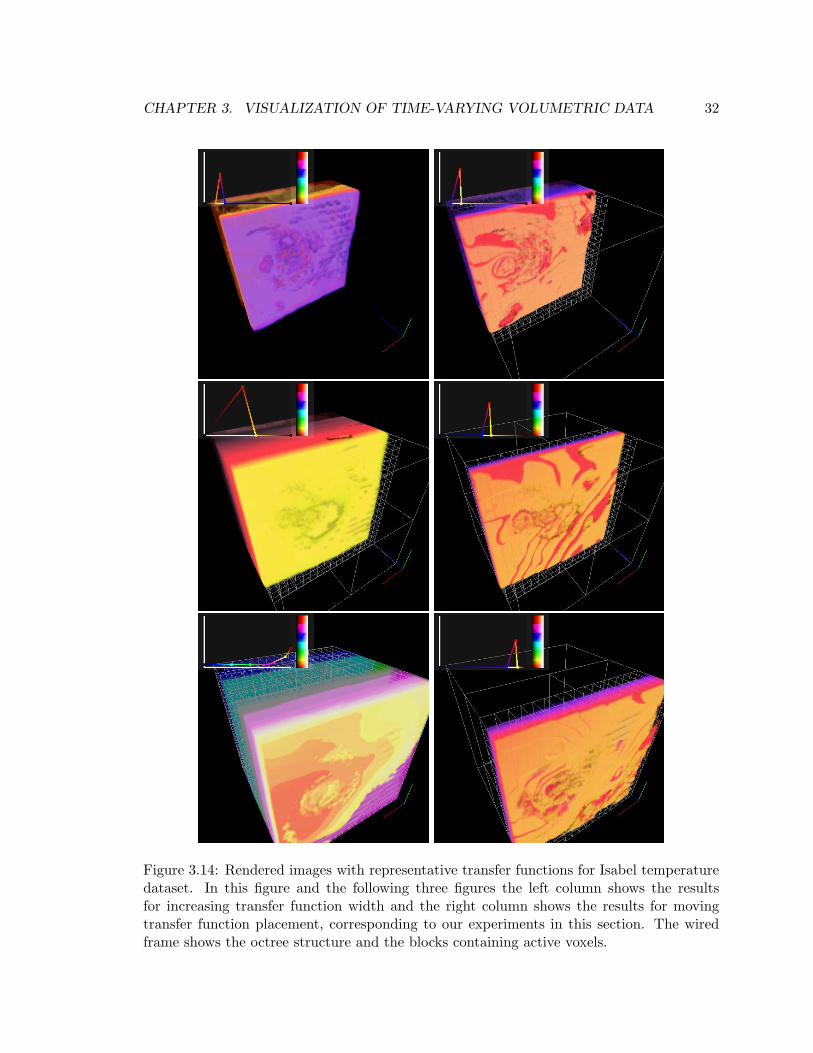
CHAPTER 3. VISUALIZATION OF TIME-VARYING VOLUMETRIC DATA 32
Figure 3.14: Rendered images with representative transfer functions for Isabel temperaturedataset. In this figure and the following three figures the left column shows the resultsfor increasing transfer function width and the right column shows the results for movingtransfer function placement, corresponding to our experiments in this section. The wiredframe shows the octree structure and the blocks containing active voxels.
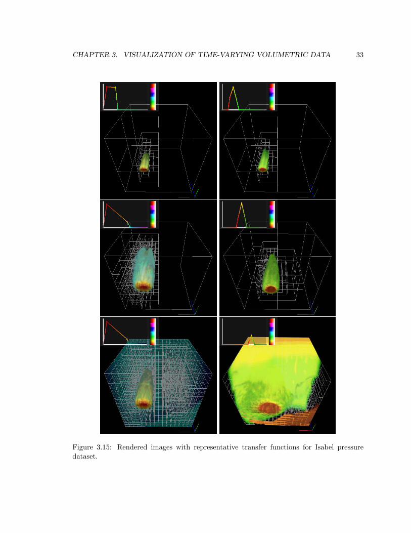
CHAPTER 3. VISUALIZATION OF TIME-VARYING VOLUMETRIC DATA 33
Figure 3.15: Rendered images with representative transfer functions for Isabel pressuredataset.
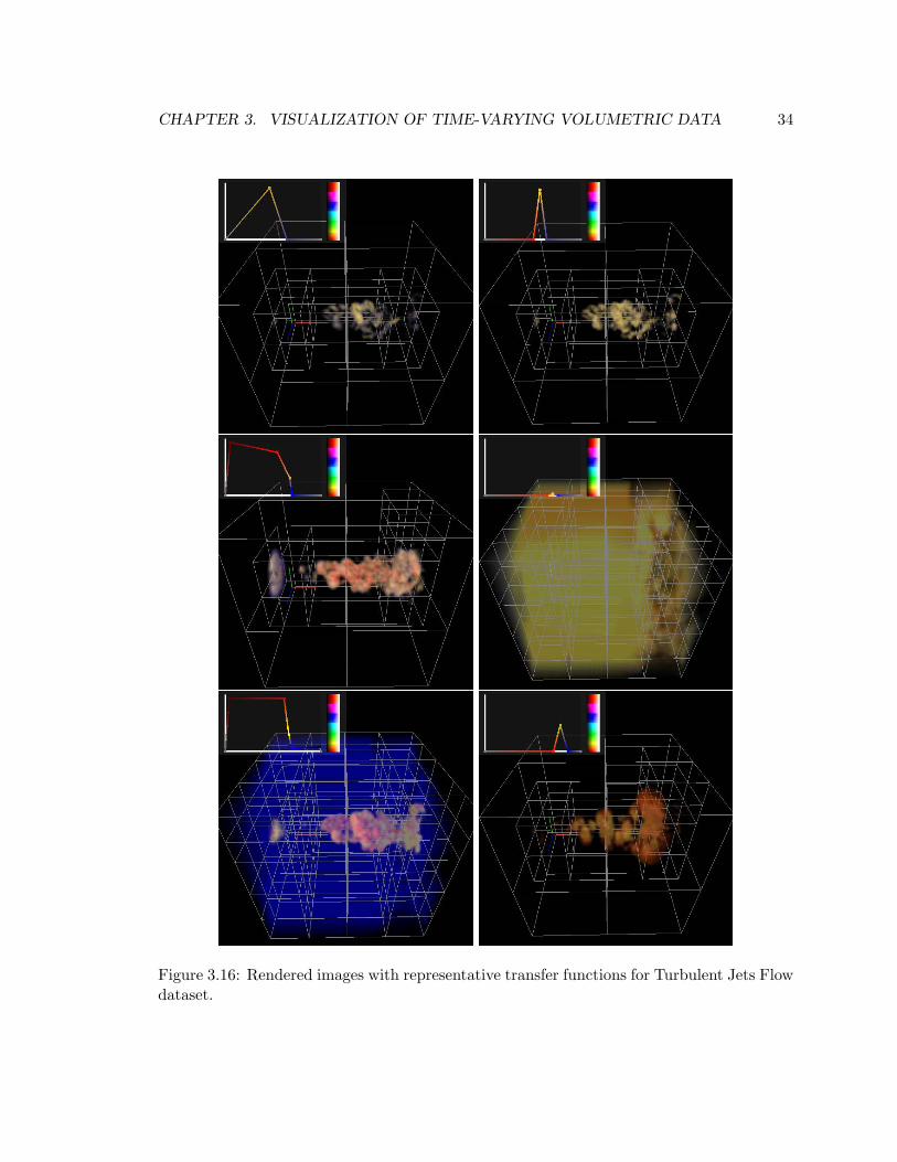
CHAPTER 3. VISUALIZATION OF TIME-VARYING VOLUMETRIC DATA 34
Figure 3.16: Rendered images with representative transfer functions for Turbulent Jets Flowdataset.
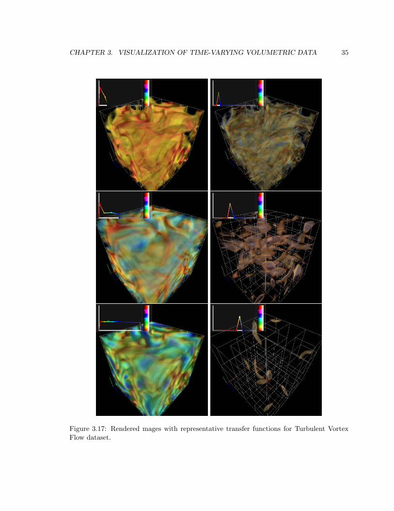
CHAPTER 3. VISUALIZATION OF TIME-VARYING VOLUMETRIC DATA 35
Figure 3.17: Rendered mages with representative transfer functions for Turbulent VortexFlow dataset.
Chapter 4
Multi-resolution Volume Rendering
In the previous chapter, we focused on the problem of large scale dataset visualization from
the aspect of dimensionality and studied time-varying datasets which consisted of multiple
time slices of 3D volumetric data. We focused on disk access performance by reducing
the data transfer from storage to main memory during user navigation. However, more
problems arise when the size of a single time step is larger than the size we can render
in an interactive rate. In such cases, a coarser resolution version of the data is chosen
for interactive frame rates. In this chapter we will be focusing on the aspect of resolution
and we will consider another common type of large scale datasets which are single frame
high-resolution three-dimensional datasets.
Scientific and medical volumetric data continues to grow in scale, and visualization in-
creasingly requires processing large amounts of data. Many methods have been proposed for
optimizing performance, especially for datasets too large to fit in main memory. One pop-
ular approach uses multi-resolution representation of the data combined with hierarchical
rendering algorithms to balance the tradeoff between quality and performance.
Multi-resolution methods typically optimize the rendering speed and memory footprints.
However, few works have addressed the question of multi-resolution visual quality, i.e., the
perceptual image quality when rendering in resolutions coarser than the original resolution
of data. In this chapter, we address the question of multi-resolution visual quality using
statistical information to decrease aliasing artifacts in direct volume rendering while using
transparent isosurfaces to decrease the loss of high-frequency features. To support this
approach, we extend previous work on branch-on-need octrees [55] to hybrid branch-on-
need octrees (HYBON), which simultaneously represent the octree structure of the samples
36
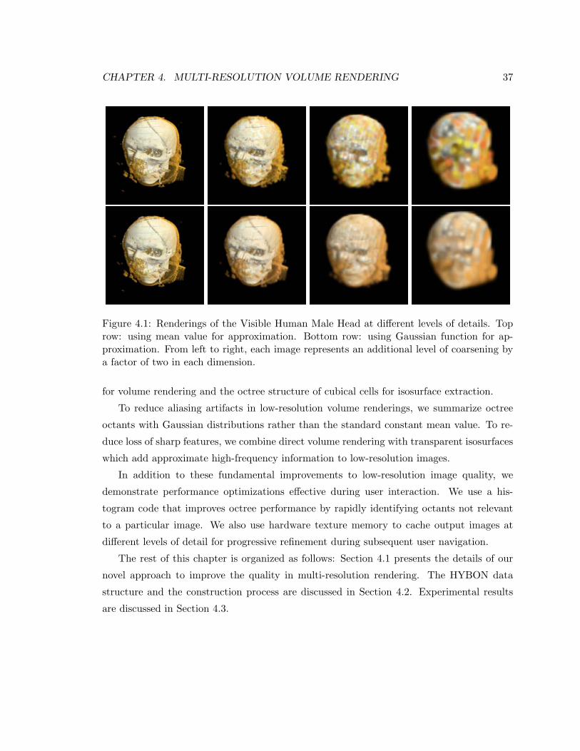
CHAPTER 4. MULTI-RESOLUTION VOLUME RENDERING 37
Figure 4.1: Renderings of the Visible Human Male Head at different levels of details. Toprow: using mean value for approximation. Bottom row: using Gaussian function for ap-proximation. From left to right, each image represents an additional level of coarsening bya factor of two in each dimension.
for volume rendering and the octree structure of cubical cells for isosurface extraction.
To reduce aliasing artifacts in low-resolution volume renderings, we summarize octree
octants with Gaussian distributions rather than the standard constant mean value. To re-
duce loss of sharp features, we combine direct volume rendering with transparent isosurfaces
which add approximate high-frequency information to low-resolution images.
In addition to these fundamental improvements to low-resolution image quality, we
demonstrate performance optimizations effective during user interaction. We use a his-
togram code that improves octree performance by rapidly identifying octants not relevant
to a particular image. We also use hardware texture memory to cache output images at
different levels of detail for progressive refinement during subsequent user navigation.
The rest of this chapter is organized as follows: Section 4.1 presents the details of our
novel approach to improve the quality in multi-resolution rendering. The HYBON data
structure and the construction process are discussed in Section 4.2. Experimental results
are discussed in Section 4.3.
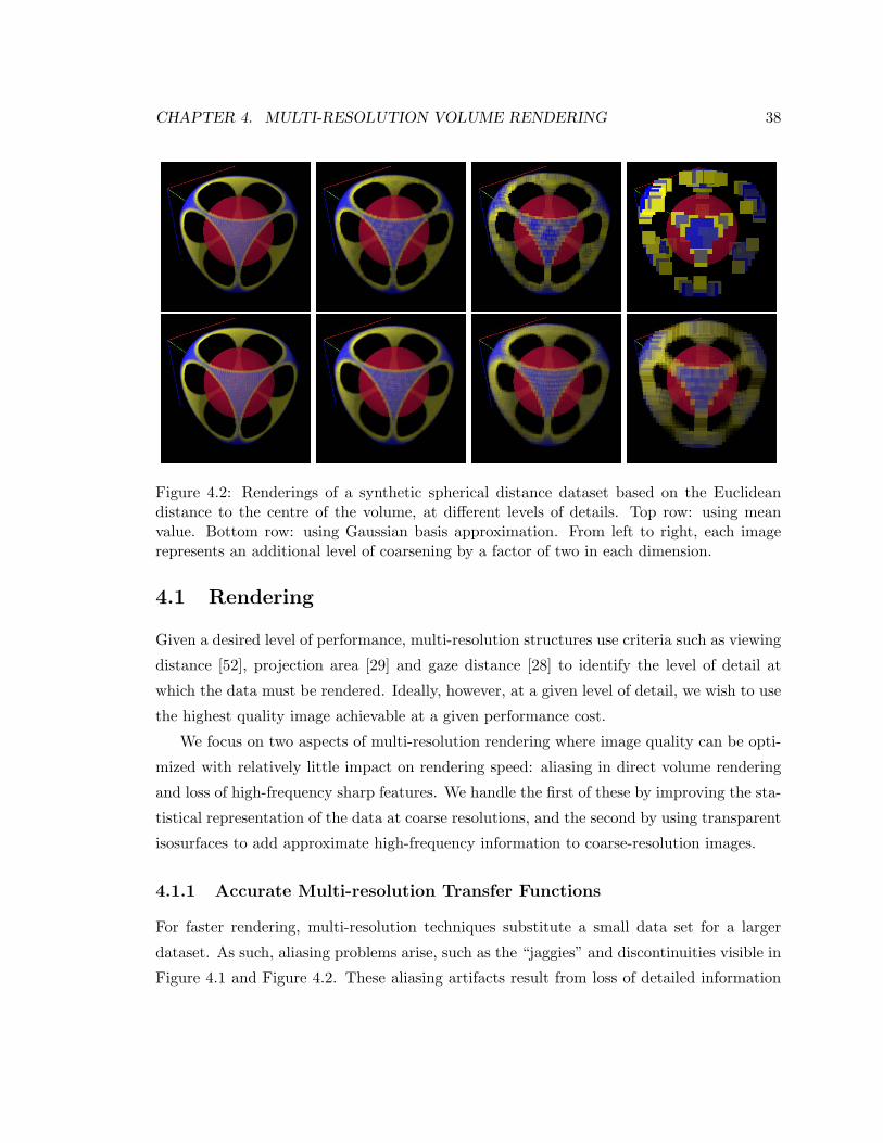
CHAPTER 4. MULTI-RESOLUTION VOLUME RENDERING 38
Figure 4.2: Renderings of a synthetic spherical distance dataset based on the Euclideandistance to the centre of the volume, at different levels of details. Top row: using meanvalue. Bottom row: using Gaussian basis approximation. From left to right, each imagerepresents an additional level of coarsening by a factor of two in each dimension.
4.1 Rendering
Given a desired level of performance, multi-resolution structures use criteria such as viewing
distance [52], projection area [29] and gaze distance [28] to identify the level of detail at
which the data must be rendered. Ideally, however, at a given level of detail, we wish to use
the highest quality image achievable at a given performance cost.
We focus on two aspects of multi-resolution rendering where image quality can be opti-
mized with relatively little impact on rendering speed: aliasing in direct volume rendering
and loss of high-frequency sharp features. We handle the first of these by improving the sta-
tistical representation of the data at coarse resolutions, and the second by using transparent
isosurfaces to add approximate high-frequency information to coarse-resolution images.
4.1.1 Accurate Multi-resolution Transfer Functions
For faster rendering, multi-resolution techniques substitute a small data set for a larger
dataset. As such, aliasing problems arise, such as the “jaggies” and discontinuities visible in
Figure 4.1 and Figure 4.2. These aliasing artifacts result from loss of detailed information
CHAPTER 4. MULTI-RESOLUTION VOLUME RENDERING 39
during construction of the multi-resolution representation. In particular, information is lost
here because the data in a subvolume is summarized with the mean of the samples in the
subvolume. This mean value is a good summary of the subvolume if the data values are
close to the mean, but is highly inaccurate when the standard deviation is relatively large.
This causes drastic problems in the resulting images because the transfer function often
does not have a smooth transition between colors and opacities for different values. More
sophisticated summaries of the subvolume can, however, be substituted for the mean, and
this idea forms the basis of our approach.
As an example, consider a subvolume with values {1, 1, 1, 1, 5, 5, 5, 5} and mean µ = 3.
Unless V (3), the color specified in the transfer function for 3, is near to the color produced
by blending V (1) and V (5), the summary information will misrepresent the data in the final
visual image.
For simplicity, we develop notation in one dimension: higher dimensions are essentially
identical, but with denser notation (i.e. integration along three dimensions). Assume that
the scalar field to be visualized is f(x), and that the sample points xi are evenly spaced:
i.e. that f(xi) = f(iT ) for some sampling distance T . For convenience, we use fi to refer
to f(xi).
Typically, the transfer function V is a vector-valued function mapping input isovalues
to output colors and opacity. We write this transfer function as V : IR → (R, G, B, α),
and state the rendering task in terms of visualizing V (f(x)), of which we only know the
values V (fi). A proper coarse visualization of this discrete dataset would involve smoothing
V (f) with a low-pass filter in order to avoid aliasing, then sub-sampling. For level n in the
multi-resolution hierarchy, this can be written as:
Vn+1(f(y)) =
∫ ∞
−∞Vn(f(y − x))w(x)dx (4.1)
where
f(x) =∞∑
k=−∞
f(k)h(x − k) (4.2)
where w is the (continuous) low-pass filter used for computing the (n + 1)st level of the
multi-resolution pyramid and h is a (continuous) interpolation filter used to reconstruct the
underlying function f from its discrete representation. The importance of Equation 4.2 in
volume rendering has been well documented by Wittenbrink et al. [56].
The formulation in Equation 4.1 is not particularly useful, as it requires recomputing
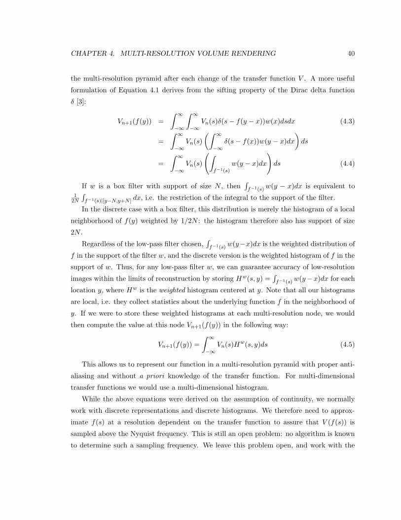
CHAPTER 4. MULTI-RESOLUTION VOLUME RENDERING 40
the multi-resolution pyramid after each change of the transfer function V . A more useful
formulation of Equation 4.1 derives from the sifting property of the Dirac delta function
δ [3]:
Vn+1(f(y)) =
∫ ∞
−∞
∫ ∞
−∞Vn(s)δ(s − f(y − x))w(x)dsdx (4.3)
=
∫ ∞
−∞Vn(s)
(∫ ∞
−∞δ(s − f(x))w(y − x)dx
)
ds
=
∫ ∞
−∞Vn(s)
(
∫
f−1(s)w(y − x)dx
)
ds (4.4)
If w is a box filter with support of size N , then∫
f−1(s) w(y − x)dx is equivalent to1
2N
∫
f−1(s)|[y−N,y+N ] dx, i.e. the restriction of the integral to the support of the filter.
In the discrete case with a box filter, this distribution is merely the histogram of a local
neighborhood of f(y) weighted by 1/2N : the histogram therefore also has support of size
2N .
Regardless of the low-pass filter chosen,∫
f−1(s) w(y−x)dx is the weighted distribution of
f in the support of the filter w, and the discrete version is the weighted histogram of f in the
support of w. Thus, for any low-pass filter w, we can guarantee accuracy of low-resolution
images within the limits of reconstruction by storing Hw(s, y) =∫
f−1(s) w(y−x)dx for each
location y, where Hw is the weighted histogram centered at y. Note that all our histograms
are local, i.e. they collect statistics about the underlying function f in the neighborhood of
y. If we were to store these weighted histograms at each multi-resolution node, we would
then compute the value at this node Vn+1(f(y)) in the following way:
Vn+1(f(y)) =
∫ ∞
−∞Vn(s)Hw(s, y)ds (4.5)
This allows us to represent our function in a multi-resolution pyramid with proper anti-
aliasing and without a priori knowledge of the transfer function. For multi-dimensional
transfer functions we would use a multi-dimensional histogram.
While the above equations were derived on the assumption of continuity, we normally
work with discrete representations and discrete histograms. We therefore need to approx-
imate f(s) at a resolution dependent on the transfer function to assure that V (f(s)) is
sampled above the Nyquist frequency. This is still an open problem: no algorithm is known
to determine such a sampling frequency. We leave this problem open, and work with the
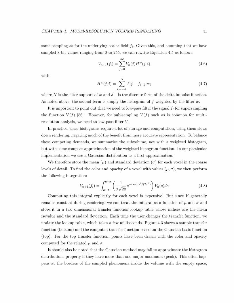
CHAPTER 4. MULTI-RESOLUTION VOLUME RENDERING 41
same sampling as for the underlying scalar field fi. Given this, and assuming that we have
sampled 8-bit values ranging from 0 to 255, we can rewrite Equation 4.5 as follows:
Vn+1(fi) =255∑
j=0
Vn(j)Hw(j, i) (4.6)
with
Hw(j, i) =N∑
k=−N
δ[j − fi−k]wk (4.7)
where N is the filter support of w and δ[ ] is the discrete form of the delta impulse function.
As noted above, the second term is simply the histogram of f weighted by the filter w.
It is important to point out that we need to low-pass filter the signal fi for supersampling
the function V (f) [56]. However, for sub-sampling V (f) such as is common for multi-
resolution analysis, we need to low-pass filter V .
In practice, since histograms require a lot of storage and computation, using them slows
down rendering, negating much of the benefit from more accurate representation. To balance
these competing demands, we summarize the subvolume, not with a weighted histogram,
but with some compact approximation of the weighted histogram function. In our particular
implementation we use a Gaussian distribution as a first approximation.
We therefore store the mean (µ) and standard deviation (σ) for each voxel in the coarse
levels of detail. To find the color and opacity of a voxel with values (µ, σ), we then perform
the following integration:
Vn+1(fi) =
∫ µ+σ
µ−σ
(
1
σ√
2πe−(s−µ)2/(2σ2)
)
Vn(s)ds (4.8)
Computing this integral explicitly for each voxel is expensive. But since V generally
remains constant during rendering, we can treat the integral as a function of µ and σ and
store it in a two dimensional transfer function lookup table whose indices are the mean
isovalue and the standard deviation. Each time the user changes the transfer function, we
update the lookup table, which takes a few milliseconds. Figure 4.3 shows a sample transfer
function (bottom) and the computed transfer function based on the Gaussian basis function
(top). For the top transfer function, points have been drawn with the color and opacity
computed for the related µ and σ.
It should also be noted that the Gaussian method may fail to approximate the histogram
distributions properly if they have more than one major maximum (peak). This often hap-
pens at the borders of the sampled phenomena inside the volume with the empty space,
CHAPTER 4. MULTI-RESOLUTION VOLUME RENDERING 42
Figure 4.3: Bottom: a transfer function with the opacities as the vertical axis (V ). Top: thecomputed Gaussian basis transfer function; The horizontal and vertical axes are respectivelymean (µ) and standard deviation (σ) and each point has been drawn with the color andopacity computed for the related µ and σ.
where a large number of voxels with priori values are included in the filtering. One solu-
tion for this case might be to use more than one Gaussian function for approximating the
distributions when the error of a single Gaussian approximation is not negligible. Although
this thesis does not addresses this approach, we use a straight forward method to solve the
problem of the empty regions, by not considering the voxels with priori values in calculating
µ and σ.
4.1.2 Translucent Isosurfaces
In addition to generating aliasing artifacts, multi-resolution rendering methods lose high-
frequency information, generating progressively blurrier views of the data, which can be
visually disconcerting. In theory, reconstruction methods can recapture the sharp features
if the data is properly sampled. Unfortunately, the very process of preparing the data
for multi-resolution rendering requires the elimination of high-frequency information in the
coarse resolutions.
To preserve at least the appearance of sharp features, we incorporate transparent iso-
surfaces in our multi-resolution renderings. By constructing sharp geometric features, this
approach has the effect of providing approximate high- resolution information without costly
reconstruction filters, improving the visual quality of the image at relatively low cost. Al-
though extracting isosurfaces itself requires interpolation and adds processing time, this can
be minimized by using octree-based methods which render a reduced number of cells de-
pending on the current resolution level. We used the Richtmyer-Meshkov instability dataset
CHAPTER 4. MULTI-RESOLUTION VOLUME RENDERING 43
(2048×2048×1920) from Lawrence Livermore National Laboratory which measures entropy
in a shock-driven instability. Figure 4.4 shows images rendered in the 5th level of coarsening
(643) and 6th level of coarsening (323) with and without isosurfaces. As it can be seen, in
the hybrid rendering of the lower level of detail Figure 4.4(d), we can perceive sharp features
that don’t appear in the direct volume rendering of the higher level of detail Figure 4.4(a).
(a) 643 (15 FPS) (b) 643 (8 FPS)
(c) 323 (78 FPS) (d) 323 (29 FPS)
Figure 4.4: Adding isosurfaces to reveal sharp features in the Richtmyer-Meshkov instabilitydataset. Left: splatting. Right: splatting + transparent isosurface.
4.1.3 Combined Isosurface and Volumetric Rendering
For correct composition of direct volume rendering and multiple shaded transparent isosur-
faces, we project the volume in sorted order [18]. We do so by processing the subvolumes in
back-to-front order and traverse the cells in each subvolume in back-to-front order. For each
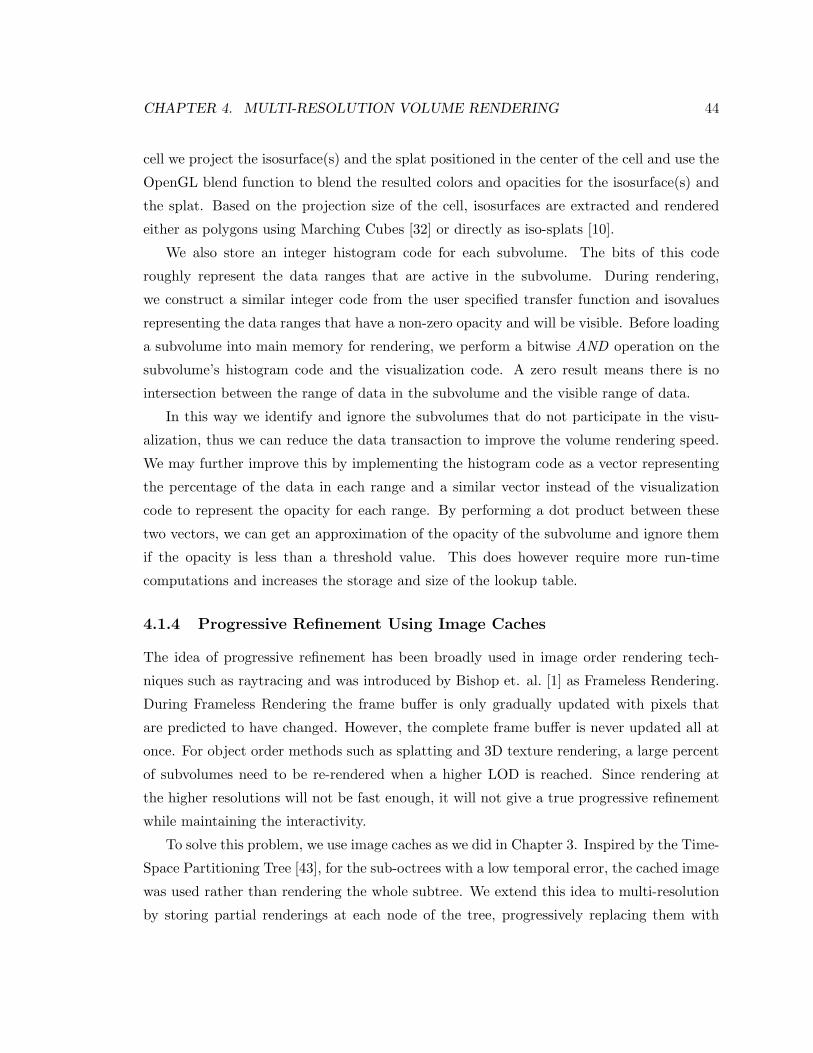
CHAPTER 4. MULTI-RESOLUTION VOLUME RENDERING 44
cell we project the isosurface(s) and the splat positioned in the center of the cell and use the
OpenGL blend function to blend the resulted colors and opacities for the isosurface(s) and
the splat. Based on the projection size of the cell, isosurfaces are extracted and rendered
either as polygons using Marching Cubes [32] or directly as iso-splats [10].
We also store an integer histogram code for each subvolume. The bits of this code
roughly represent the data ranges that are active in the subvolume. During rendering,
we construct a similar integer code from the user specified transfer function and isovalues
representing the data ranges that have a non-zero opacity and will be visible. Before loading
a subvolume into main memory for rendering, we perform a bitwise AND operation on the
subvolume’s histogram code and the visualization code. A zero result means there is no
intersection between the range of data in the subvolume and the visible range of data.
In this way we identify and ignore the subvolumes that do not participate in the visu-
alization, thus we can reduce the data transaction to improve the volume rendering speed.
We may further improve this by implementing the histogram code as a vector representing
the percentage of the data in each range and a similar vector instead of the visualization
code to represent the opacity for each range. By performing a dot product between these
two vectors, we can get an approximation of the opacity of the subvolume and ignore them
if the opacity is less than a threshold value. This does however require more run-time
computations and increases the storage and size of the lookup table.
4.1.4 Progressive Refinement Using Image Caches
The idea of progressive refinement has been broadly used in image order rendering tech-
niques such as raytracing and was introduced by Bishop et. al. [1] as Frameless Rendering.
During Frameless Rendering the frame buffer is only gradually updated with pixels that
are predicted to have changed. However, the complete frame buffer is never updated all at
once. For object order methods such as splatting and 3D texture rendering, a large percent
of subvolumes need to be re-rendered when a higher LOD is reached. Since rendering at
the higher resolutions will not be fast enough, it will not give a true progressive refinement
while maintaining the interactivity.
To solve this problem, we use image caches as we did in Chapter 3. Inspired by the Time-
Space Partitioning Tree [43], for the sub-octrees with a low temporal error, the cached image
was used rather than rendering the whole subtree. We extend this idea to multi-resolution
by storing partial renderings at each node of the tree, progressively replacing them with
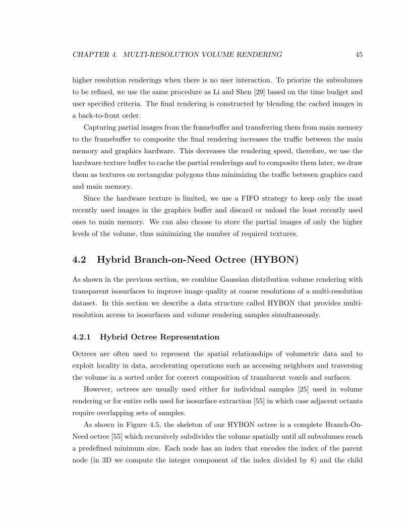
CHAPTER 4. MULTI-RESOLUTION VOLUME RENDERING 45
higher resolution renderings when there is no user interaction. To priorize the subvolumes
to be refined, we use the same procedure as Li and Shen [29] based on the time budget and
user specified criteria. The final rendering is constructed by blending the cached images in
a back-to-front order.
Capturing partial images from the framebuffer and transferring them from main memory
to the framebuffer to composite the final rendering increases the traffic between the main
memory and graphics hardware. This decreases the rendering speed, therefore, we use the
hardware texture buffer to cache the partial renderings and to composite them later, we draw
them as textures on rectangular polygons thus minimizing the traffic between graphics card
and main memory.
Since the hardware texture is limited, we use a FIFO strategy to keep only the most
recently used images in the graphics buffer and discard or unload the least recently used
ones to main memory. We can also choose to store the partial images of only the higher
levels of the volume, thus minimizing the number of required textures.
4.2 Hybrid Branch-on-Need Octree (HYBON)
As shown in the previous section, we combine Gaussian distribution volume rendering with
transparent isosurfaces to improve image quality at coarse resolutions of a multi-resolution
dataset. In this section we describe a data structure called HYBON that provides multi-
resolution access to isosurfaces and volume rendering samples simultaneously.
4.2.1 Hybrid Octree Representation
Octrees are often used to represent the spatial relationships of volumetric data and to
exploit locality in data, accelerating operations such as accessing neighbors and traversing
the volume in a sorted order for correct composition of translucent voxels and surfaces.
However, octrees are usually used either for individual samples [25] used in volume
rendering or for entire cells used for isosurface extraction [55] in which case adjacent octants
require overlapping sets of samples.
As shown in Figure 4.5, the skeleton of our HYBON octree is a complete Branch-On-
Need octree [55] which recursively subdivides the volume spatially until all subvolumes reach
a predefined minimum size. Each node has an index that encodes the index of the parent
node (in 3D we compute the integer component of the index divided by 8) and the child
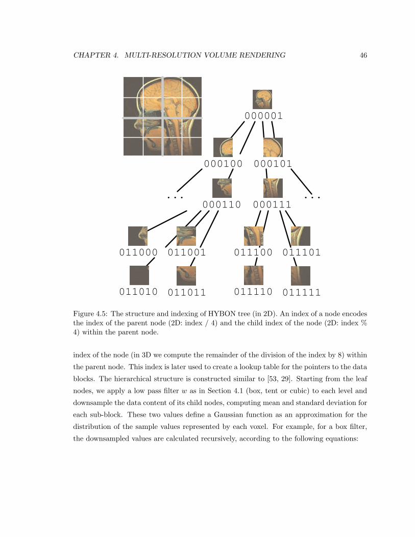
CHAPTER 4. MULTI-RESOLUTION VOLUME RENDERING 46
000001
000100 000101
000110 000111
011000 011001
011010 011011
011100 011101
011110 011111
......
Figure 4.5: The structure and indexing of HYBON tree (in 2D). An index of a node encodesthe index of the parent node (2D: index / 4) and the child index of the node (2D: index %4) within the parent node.
index of the node (in 3D we compute the remainder of the division of the index by 8) within
the parent node. This index is later used to create a lookup table for the pointers to the data
blocks. The hierarchical structure is constructed similar to [53, 29]. Starting from the leaf
nodes, we apply a low pass filter w as in Section 4.1 (box, tent or cubic) to each level and
downsample the data content of its child nodes, computing mean and standard deviation for
each sub-block. These two values define a Gaussian function as an approximation for the
distribution of the sample values represented by each voxel. For example, for a box filter,
the downsampled values are calculated recursively, according to the following equations:
CHAPTER 4. MULTI-RESOLUTION VOLUME RENDERING 47
cell
subvolume
voxel
null
Figure 4.6: Creating cell structures in subvolumes by overlapping border voxels.
µ =8∑
i=1
µi
8(4.9)
σ2 =N∑
i=1
(xi − µ)2
N(4.10)
=8∑
j=i
(µi + σi − µ)2 + (µi − σi − µ)2
2 × 8(4.11)
=1
8
8∑
i=1
(µi − µ)2 + σ2i (4.12)
In addition to the mean and standard deviation, we also precompute the normals in each
octant and quantize them as normalized vectors in polar coordinates.
The octree as described so far captures a multi-resolution version of the samples for vol-
ume rendering. For isosurface extraction, we add a cell-based structure in each subvolume.
As shown in Figure 4.6, to avoid cracks between the surfaces extracted from neighboring
subvolumes at the same level of detail, we copy the data points shared on the boundaries of
adjacent subvolumes.
CHAPTER 4. MULTI-RESOLUTION VOLUME RENDERING 48
4.2.2 Hybrid Octree Optimization
For rapid identification of octree cells that need to be rendered at a particular level of detail,
we apply a modified version of the span space scheme [44]. Instead of storing a minimum
and maximum isovalue for the cell, we store a quantized histogram code based on dividing
the isovalue range of the data into 32 equal bins. The isovalue span of a given cell will either
intersect a given bin or not, resulting in 32 single bits which we pack into a 32 bit variable
to compute the histogram code. At render time, we simply compute the bin into which an
isovalue of interest falls and compare the appropriate histogram code with the code for each
cell. Cells for which the corresponding bit is not set are guaranteed not to be needed for
rendering, and are immediately discarded.
Compared with a straightforward span space implementation, this histogram code has
two advantages: first, it replaces two comparisons with a single bitwise comparison, and
second, it permits simultaneous testing for a range of isovalues rather than a single isovalue.
Since we support the extraction of multiple transparent isosurfaces and generate a volume
rendering simultaneously, this significantly reduces the computation needed to determine
whether any subvolume in the octree needs processing.
As an additional optimization, we compress uniform regions of the data by setting a
threshold ε ≥ 0, and replacing any subvolume in the octree whose standard deviation is
less than ε with a single leaf node. Performed recursively through the octree, this has the
effect of compressing any large regions of little isovalue change to single entries in the octree,
again increasing rendering speed. We store the compressed data blocks containing the mean,
standard deviation and discretized normal vector, along with an lookup table that contains
pointers to the data blocks and the histogram code for each block.
Since the same partitioning policy is used in both pre-processing and run time, the
octree structure can be computed in run time for a volume with a certain resolution. In run
time, knowing a voxel’s spatial location and the level-of-detail, we can identify the index of
the block (Figure 4.5) containing that voxel. The lookup function converts the index to a
sequence number (to avoid redundant lookup entries in the table) and the sequence number
is used to get the histogram code and the pointer to the data block (or the offset to the
data block in the data file) from the lookup table. A null pointer shows the block has been
discarded in the preprocessing step. The histogram code is compared with the visualization
code (Section 4.1.3) and the data block is loaded, uncompressed and rendered if required.
CHAPTER 4. MULTI-RESOLUTION VOLUME RENDERING 49
4.3 Implementation and Results
We have implemented our HYBON data structure and our algorithms for high-quality multi-
resolution rendering on a 3.06 GHz Intel Xeon PC with 2 GB of main memory and an nVidia
AGP 8x GeForce 6800 graphics card. For evaluation purposes, we used three representative
datasets: a synthetic dataset, a medical dataset, and a fluid dynamics simulation dataset.
The synthetic dataset is a spherical distance function sampled at a resolution of 2563,
while the medical dataset is the visible human male CT dataset with a resolution of 512 ×512× 1878, and the simulation dataset is one frame (frame 250) of the Richtmyer-Meshkov
instability dataset from Lawrence Livermore National Laboratory which has a resolution of
2048 × 2048 × 1920.
Since the goal of our work was to provide higher-quality renderings at coarse resolutions
of a multi-resolution dataset, our first concern was the relative quality of the downsampling
and of the resultant images. We tested this by comparing V ◦ f , the function f with
transfer function V applied to it at coarse levels of resolution using three low-pass filters
for downsampling and under three different downsampling distributions. We used box, tent
(linear) and cubic (spline) low-pass filters for downsampling. The three distributions we
tested were mean (i.e. traditional BON downsampling), Gaussian distribution (mean +
standard deviation), and full filtered histogram as a benchmark to compare the former two
distributions with. Including the full histogram adds a huge overhead of 256 floating point
(or 4 byte integer) numbers per voxel (1KB) and storing the full datasets required much
more memory than our machine had available. Since it was not possible to perform the
tests at full resolution, we instead performed it at maximum resolutions of 643 and lower
for each of the datasets.
We performed two tests with the spherical distance function to illustrate the relationship
between the transfer function and the quality of the downsampling distribution. In the first
test, we applied a high-frequency transfer function which rapidly alternated between red,
green and blue, and in the second, we applied a lower-frequency transfer function which
also alternated between red, green and blue. Figure 4.7 shows these transfer functions for
reference. Each set of tests was repeated for box, tent and cubic filters for downsampling.
We show our rendering results in Figure 4.8 through Figure 4.25. In each of these figures,
the left column is the most accurate distribution: the histogram distribution, while the mid-
dle column is the Gaussian distribution, and the right column the least accurate: the mean
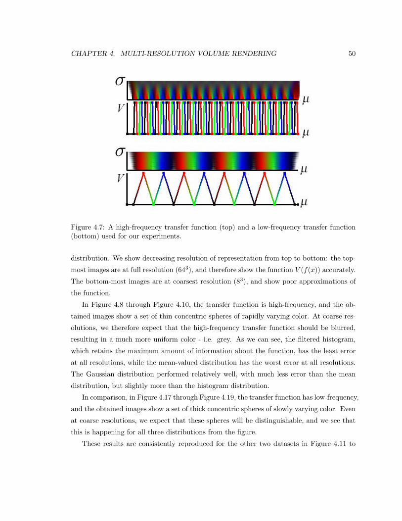
CHAPTER 4. MULTI-RESOLUTION VOLUME RENDERING 50
Figure 4.7: A high-frequency transfer function (top) and a low-frequency transfer function(bottom) used for our experiments.
distribution. We show decreasing resolution of representation from top to bottom: the top-
most images are at full resolution (643), and therefore show the function V (f(x)) accurately.
The bottom-most images are at coarsest resolution (83), and show poor approximations of
the function.
In Figure 4.8 through Figure 4.10, the transfer function is high-frequency, and the ob-
tained images show a set of thin concentric spheres of rapidly varying color. At coarse res-
olutions, we therefore expect that the high-frequency transfer function should be blurred,
resulting in a much more uniform color - i.e. grey. As we can see, the filtered histogram,
which retains the maximum amount of information about the function, has the least error
at all resolutions, while the mean-valued distribution has the worst error at all resolutions.
The Gaussian distribution performed relatively well, with much less error than the mean
distribution, but slightly more than the histogram distribution.
In comparison, in Figure 4.17 through Figure 4.19, the transfer function has low-frequency,
and the obtained images show a set of thick concentric spheres of slowly varying color. Even
at coarse resolutions, we expect that these spheres will be distinguishable, and we see that
this is happening for all three distributions from the figure.
These results are consistently reproduced for the other two datasets in Figure 4.11 to
CHAPTER 4. MULTI-RESOLUTION VOLUME RENDERING 51
Figure 4.16 (high-frequency transfer function) and Figure 4.20 to Figure 4.25 (low-frequency
transfer function), in which the histogram distribution consistently gives the best results,
the mean distribution the worst, and the Gaussian distribution good but not quite perfect
results.
For an analytic evaluation of the error of our approximation we plotted the root mean
squared error of mean and Gaussian approximations of the histogram distribution as the
benchmark. We computed the difference between the approximated distribution of f for each
voxel and the histogram distribution for the same voxel. As Figure 4.26 shows, the error of
the Gaussian approximation was consistently less than the error of the mean approximation
at each level of resolution, with the error usually diminishing under the Gaussian distribution
as the resolution was coarsened further. This usually occurs because the downsampled voxels
represent progressively more of the original data, with a Gaussian distribution becoming a
better fit to the data as more samples accumulate. Although using different low-pass filters,
effects the visual quality in coarser levels of detail (cubic better than linear, and linear better
that box), however it does not have a major effect on the approximations errors. This is
because the filters are not supposed to necessarily change the histograms to become more
close to Gaussian distributions.
To evaluate the effect of the Gaussian approximation on rendering, we calculated the
root mean squared error in each voxel of the function f after application of the transfer
function V . We computed the RGBA color of each voxel using the Gaussian approxima-
tion and mean approximation and compared it to the color when using the full histogram
distribution for that voxel, averaging the root mean squared errors of red, green, blue and
alpha components. A perceptual color space such as CIE Lab might be a better basis for
an insightful comparison. The results are presented in Figure 4.27 for the high-frequency
transfer function and Figure 4.28 for low-frequency transfer function. Again, as we had
already expected from the rendered figures, the average error of rendering is consistently
less for the Gaussian distribution than the mean distribution.
4.3.1 Memory and storage overhead
It is expected that encoding the standard deviation values for each voxel would add around
25% (1-byte σ added to 1-byte µ + 2-bytes gradient) overhead in terms of memory and
processing power. Surprisingly there was no significant memory or processing overhead,
presumably due to compiler optimization of data structures. Since voxel value (1 byte
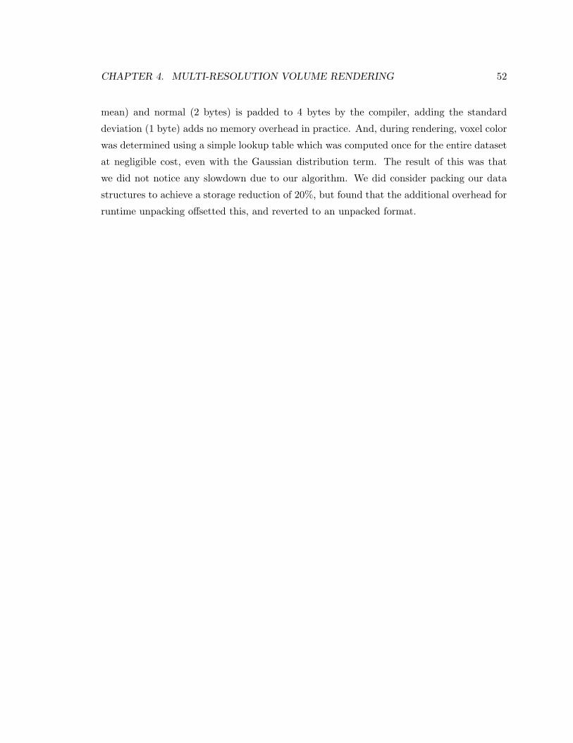
CHAPTER 4. MULTI-RESOLUTION VOLUME RENDERING 52
mean) and normal (2 bytes) is padded to 4 bytes by the compiler, adding the standard
deviation (1 byte) adds no memory overhead in practice. And, during rendering, voxel color
was determined using a simple lookup table which was computed once for the entire dataset
at negligible cost, even with the Gaussian distribution term. The result of this was that
we did not notice any slowdown due to our algorithm. We did consider packing our data
structures to achieve a storage reduction of 20%, but found that the additional overhead for
runtime unpacking offsetted this, and reverted to an unpacked format.
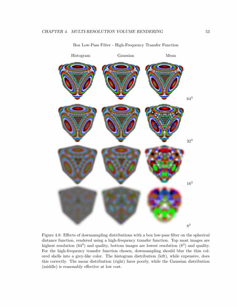
CHAPTER 4. MULTI-RESOLUTION VOLUME RENDERING 53
Box Low-Pass Filter - High-Frequency Transfer Function
Histogram Gaussian Mean
643
323
163
83
Figure 4.8: Effects of downsampling distributions with a box low-pass filter on the sphericaldistance function, rendered using a high-frequency transfer function. Top most images arehighest resolution (643) and quality, bottom images are lowest resolution (83) and quality.For the high-frequency transfer function chosen, downsampling should blur the thin col-ored shells into a grey-like color. The histogram distribution (left), while expensive, doesthis correctly. The mean distribution (right) fares poorly, while the Gaussian distribution(middle) is reasonably effective at low cost.
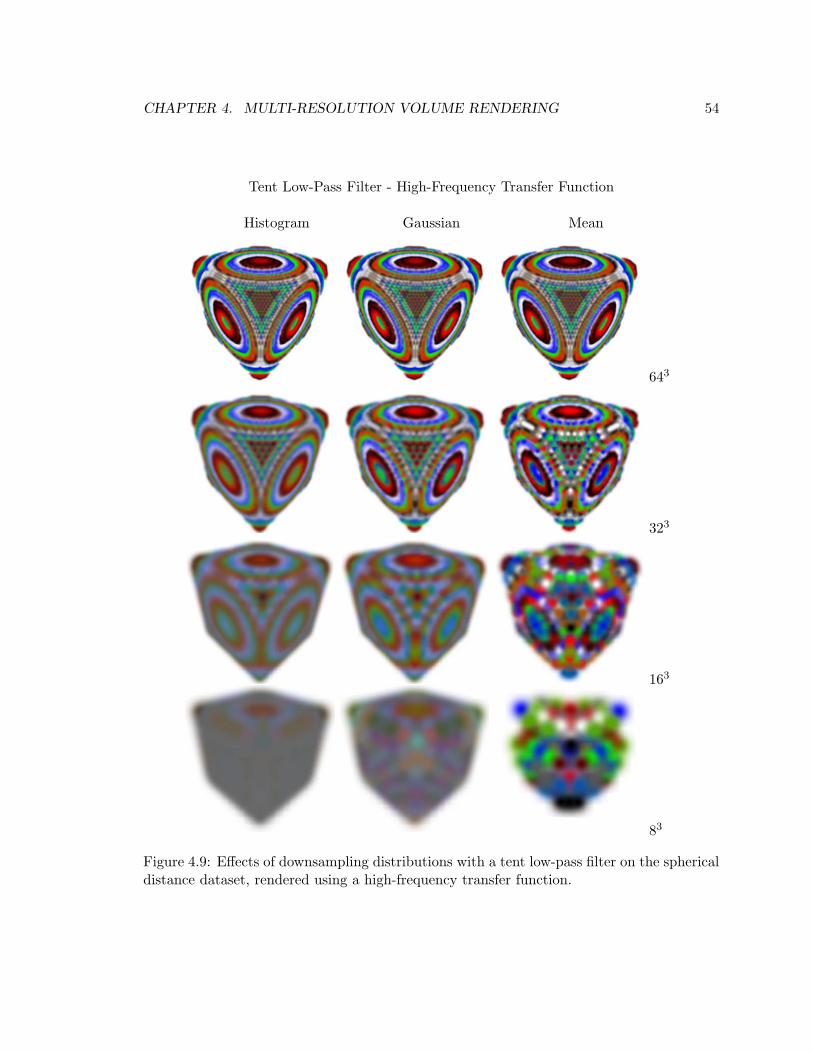
CHAPTER 4. MULTI-RESOLUTION VOLUME RENDERING 54
Tent Low-Pass Filter - High-Frequency Transfer Function
Histogram Gaussian Mean
643
323
163
83
Figure 4.9: Effects of downsampling distributions with a tent low-pass filter on the sphericaldistance dataset, rendered using a high-frequency transfer function.
CHAPTER 4. MULTI-RESOLUTION VOLUME RENDERING 55
Cubic Low-Pass Filter - High-Frequency Transfer Function
Histogram Gaussian Mean
643
323
163
83
Figure 4.10: Effects of downsampling distributions with a cubic low-pass filter on the spher-ical distance dataset, rendered using a high-frequency transfer function.
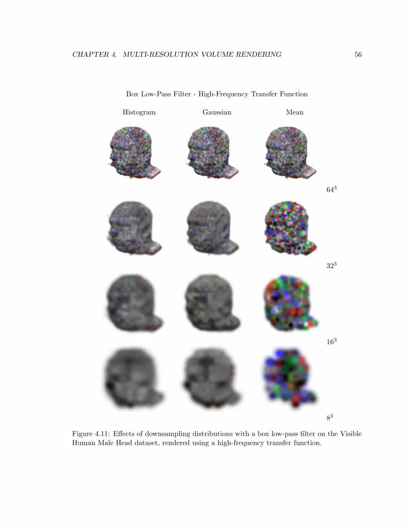
CHAPTER 4. MULTI-RESOLUTION VOLUME RENDERING 56
Box Low-Pass Filter - High-Frequency Transfer Function
Histogram Gaussian Mean
643
323
163
83
Figure 4.11: Effects of downsampling distributions with a box low-pass filter on the VisibleHuman Male Head dataset, rendered using a high-frequency transfer function.
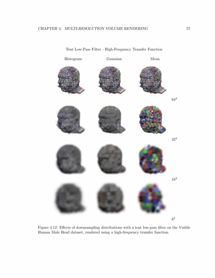
CHAPTER 4. MULTI-RESOLUTION VOLUME RENDERING 57
Tent Low-Pass Filter - High-Frequency Transfer Function
Histogram Gaussian Mean
643
323
163
83
Figure 4.12: Effects of downsampling distributions with a tent low-pass filter on the VisibleHuman Male Head dataset, rendered using a high-frequency transfer function.
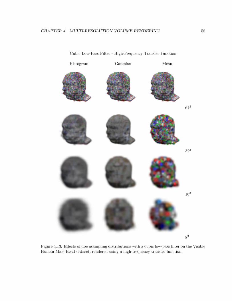
CHAPTER 4. MULTI-RESOLUTION VOLUME RENDERING 58
Cubic Low-Pass Filter - High-Frequency Transfer Function
Histogram Gaussian Mean
643
323
163
83
Figure 4.13: Effects of downsampling distributions with a cubic low-pass filter on the VisibleHuman Male Head dataset, rendered using a high-frequency transfer function.
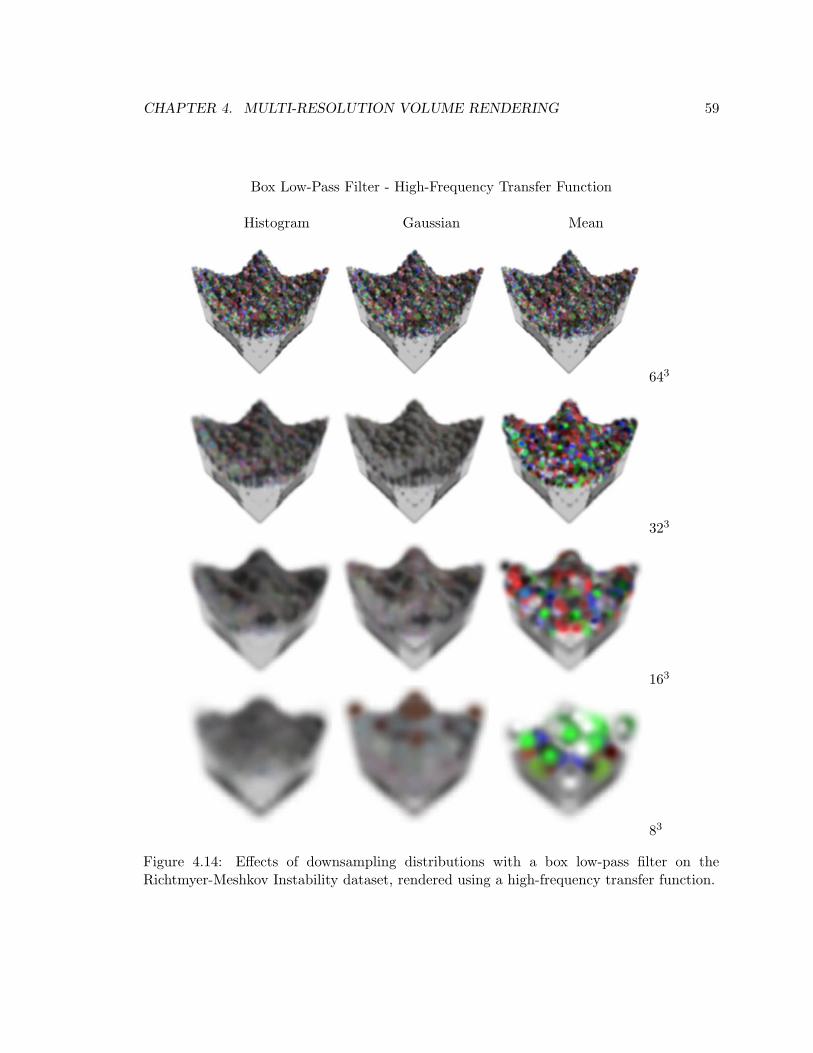
CHAPTER 4. MULTI-RESOLUTION VOLUME RENDERING 59
Box Low-Pass Filter - High-Frequency Transfer Function
Histogram Gaussian Mean
643
323
163
83
Figure 4.14: Effects of downsampling distributions with a box low-pass filter on theRichtmyer-Meshkov Instability dataset, rendered using a high-frequency transfer function.
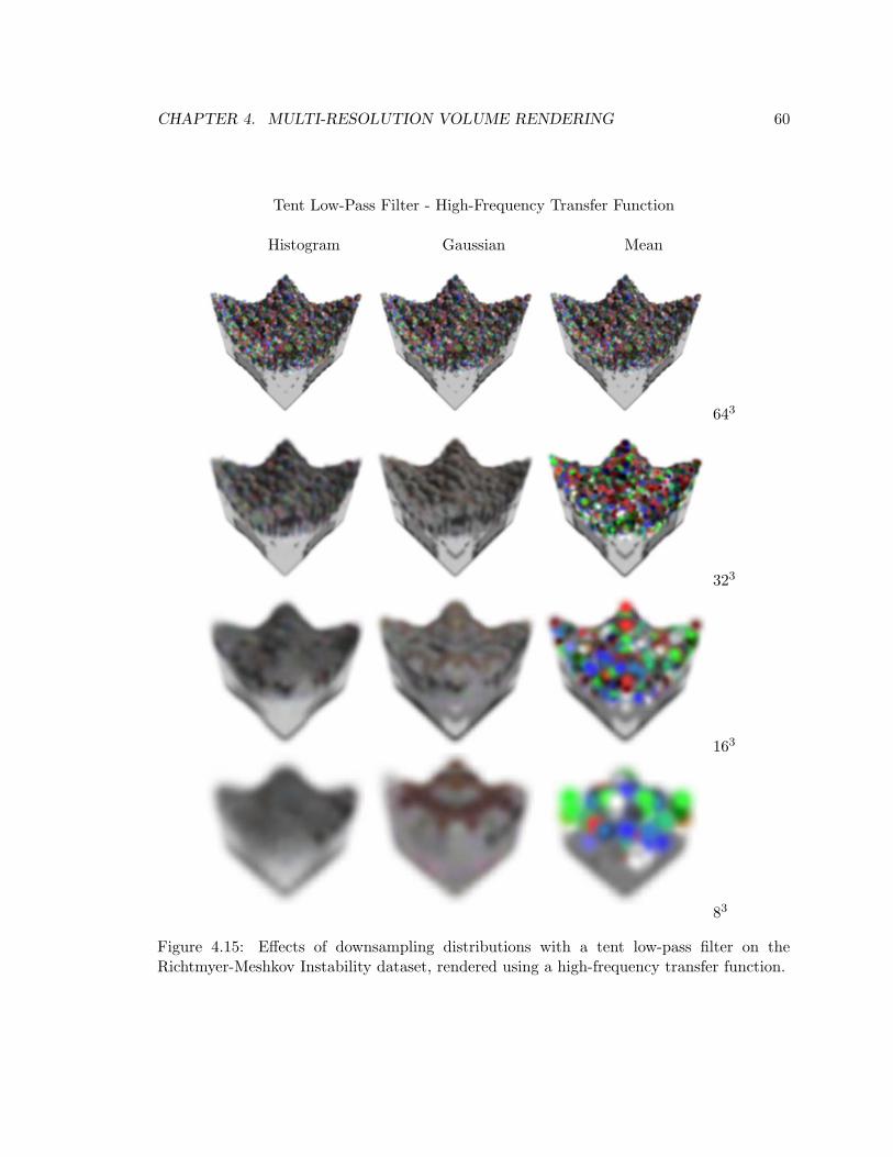
CHAPTER 4. MULTI-RESOLUTION VOLUME RENDERING 60
Tent Low-Pass Filter - High-Frequency Transfer Function
Histogram Gaussian Mean
643
323
163
83
Figure 4.15: Effects of downsampling distributions with a tent low-pass filter on theRichtmyer-Meshkov Instability dataset, rendered using a high-frequency transfer function.
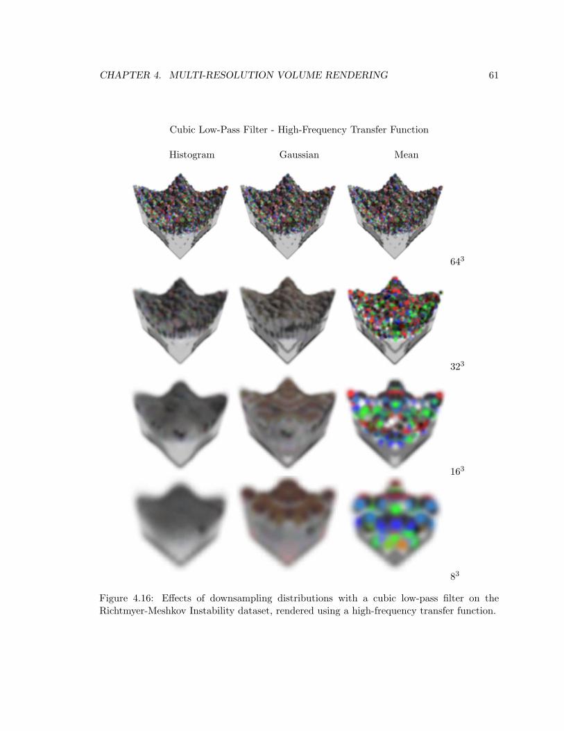
CHAPTER 4. MULTI-RESOLUTION VOLUME RENDERING 61
Cubic Low-Pass Filter - High-Frequency Transfer Function
Histogram Gaussian Mean
643
323
163
83
Figure 4.16: Effects of downsampling distributions with a cubic low-pass filter on theRichtmyer-Meshkov Instability dataset, rendered using a high-frequency transfer function.
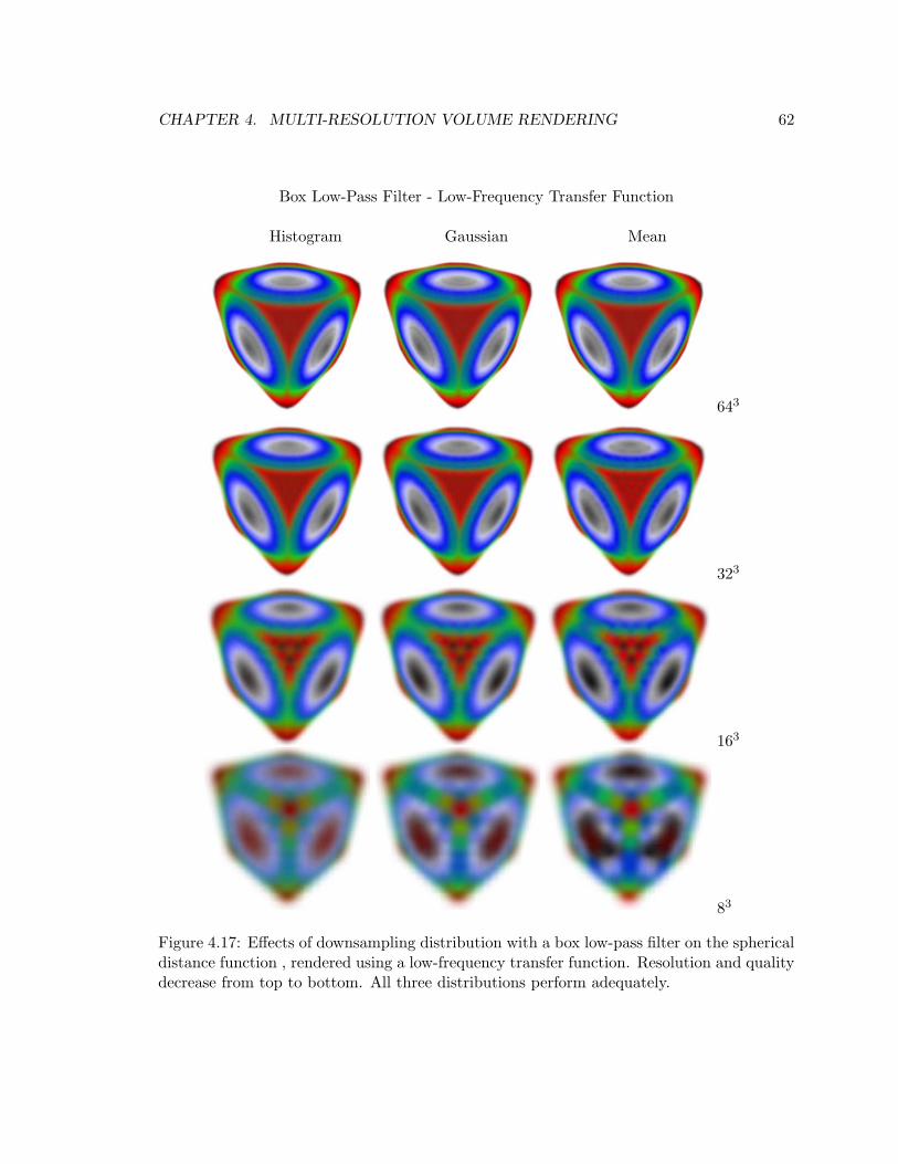
CHAPTER 4. MULTI-RESOLUTION VOLUME RENDERING 62
Box Low-Pass Filter - Low-Frequency Transfer Function
Histogram Gaussian Mean
643
323
163
83
Figure 4.17: Effects of downsampling distribution with a box low-pass filter on the sphericaldistance function , rendered using a low-frequency transfer function. Resolution and qualitydecrease from top to bottom. All three distributions perform adequately.
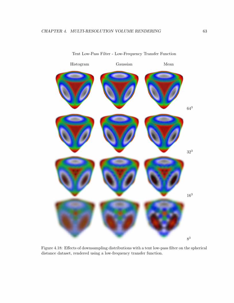
CHAPTER 4. MULTI-RESOLUTION VOLUME RENDERING 63
Tent Low-Pass Filter - Low-Frequency Transfer Function
Histogram Gaussian Mean
643
323
163
83
Figure 4.18: Effects of downsampling distributions with a tent low-pass filter on the sphericaldistance dataset, rendered using a low-frequency transfer function.
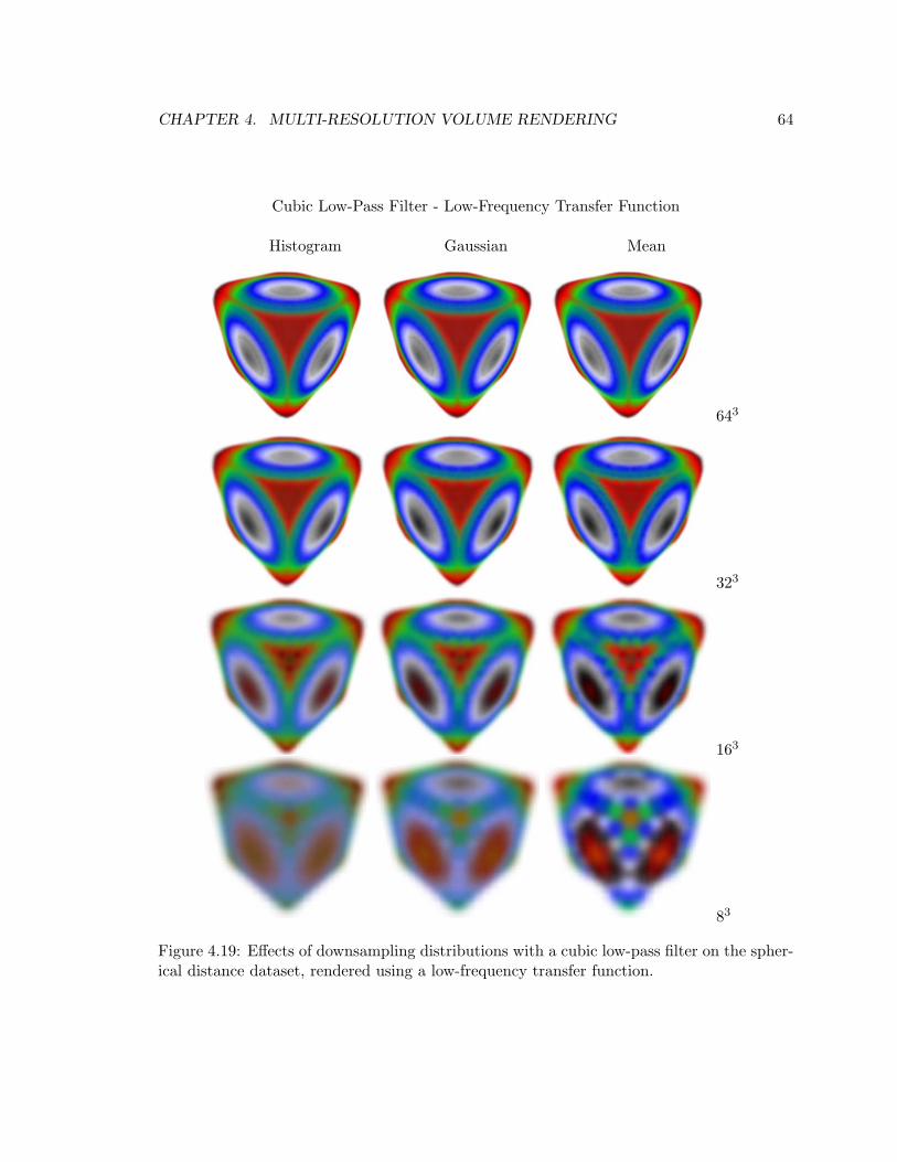
CHAPTER 4. MULTI-RESOLUTION VOLUME RENDERING 64
Cubic Low-Pass Filter - Low-Frequency Transfer Function
Histogram Gaussian Mean
643
323
163
83
Figure 4.19: Effects of downsampling distributions with a cubic low-pass filter on the spher-ical distance dataset, rendered using a low-frequency transfer function.
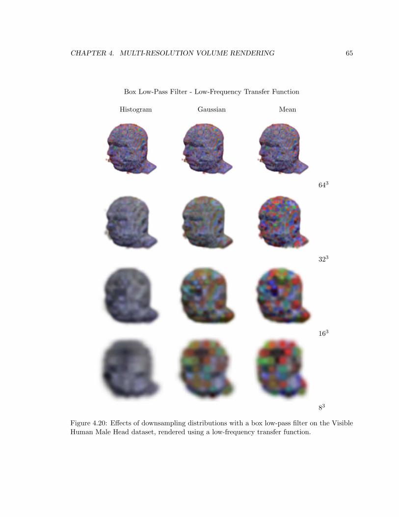
CHAPTER 4. MULTI-RESOLUTION VOLUME RENDERING 65
Box Low-Pass Filter - Low-Frequency Transfer Function
Histogram Gaussian Mean
643
323
163
83
Figure 4.20: Effects of downsampling distributions with a box low-pass filter on the VisibleHuman Male Head dataset, rendered using a low-frequency transfer function.
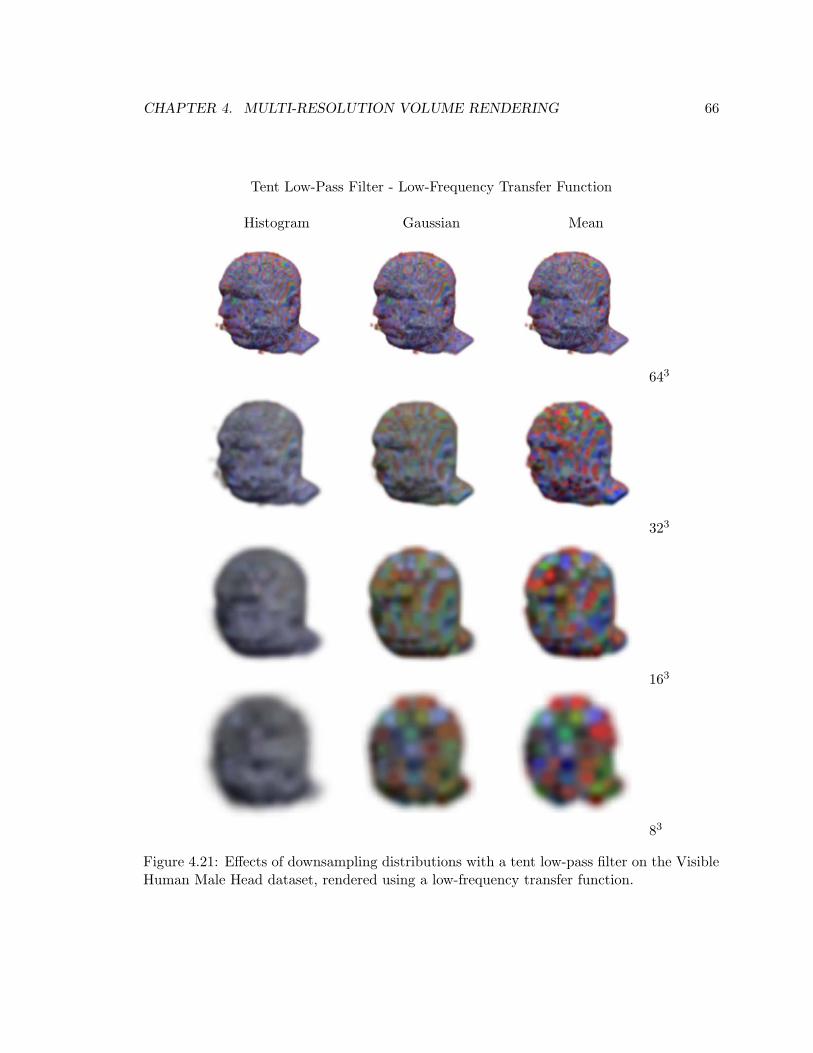
CHAPTER 4. MULTI-RESOLUTION VOLUME RENDERING 66
Tent Low-Pass Filter - Low-Frequency Transfer Function
Histogram Gaussian Mean
643
323
163
83
Figure 4.21: Effects of downsampling distributions with a tent low-pass filter on the VisibleHuman Male Head dataset, rendered using a low-frequency transfer function.
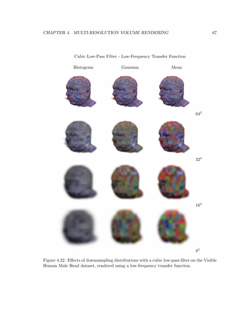
CHAPTER 4. MULTI-RESOLUTION VOLUME RENDERING 67
Cubic Low-Pass Filter - Low-Frequency Transfer Function
Histogram Gaussian Mean
643
323
163
83
Figure 4.22: Effects of downsampling distributions with a cubic low-pass filter on the VisibleHuman Male Head dataset, rendered using a low-frequency transfer function.
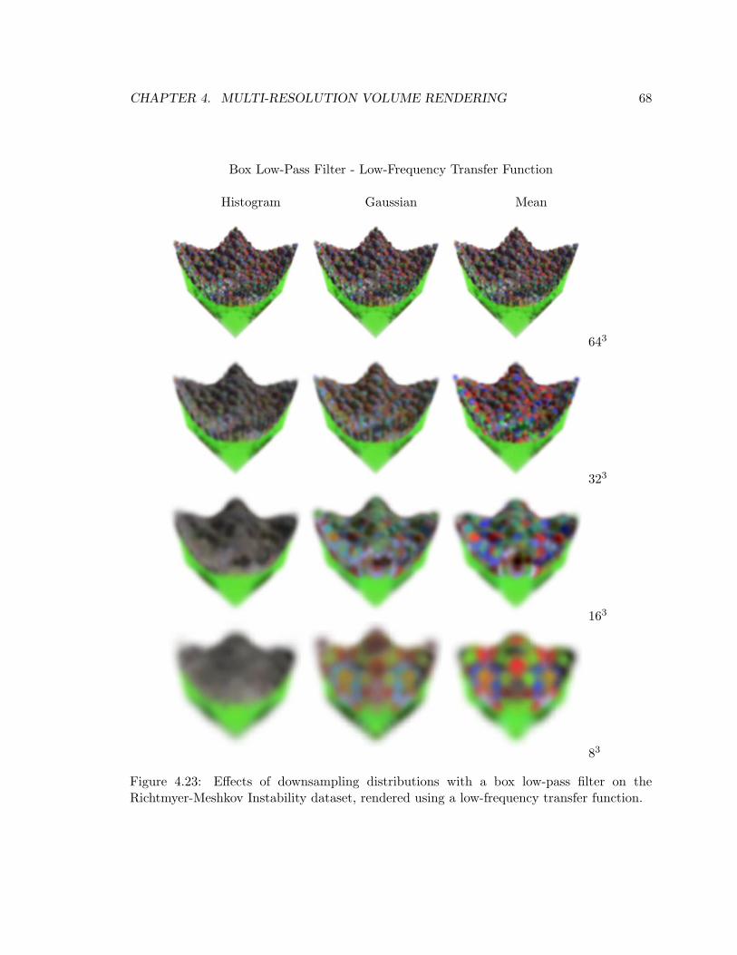
CHAPTER 4. MULTI-RESOLUTION VOLUME RENDERING 68
Box Low-Pass Filter - Low-Frequency Transfer Function
Histogram Gaussian Mean
643
323
163
83
Figure 4.23: Effects of downsampling distributions with a box low-pass filter on theRichtmyer-Meshkov Instability dataset, rendered using a low-frequency transfer function.
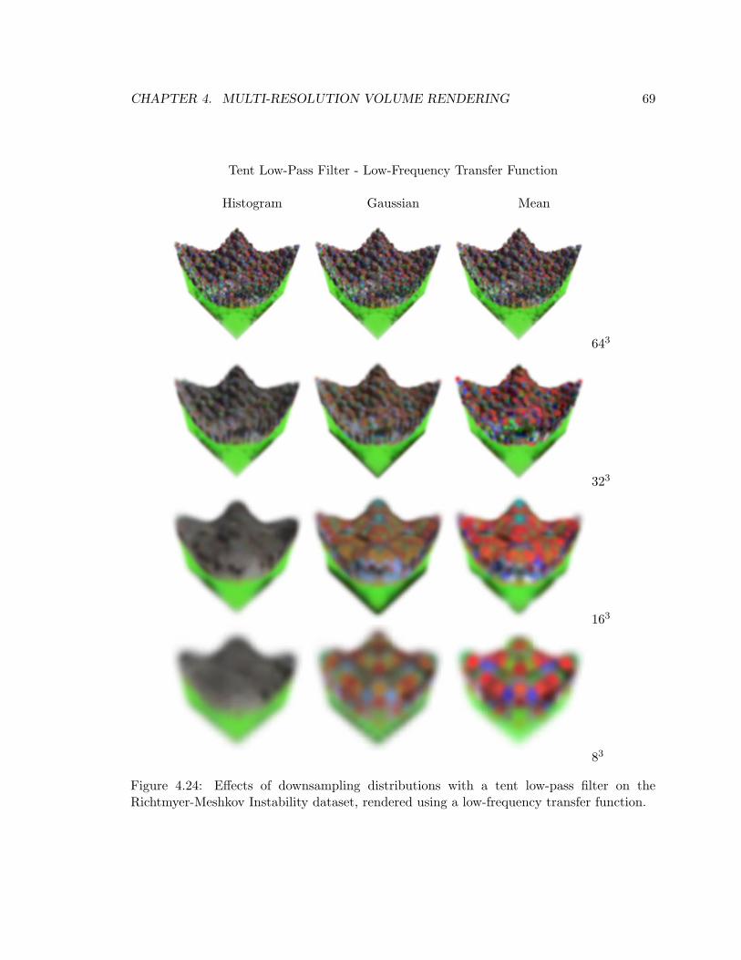
CHAPTER 4. MULTI-RESOLUTION VOLUME RENDERING 69
Tent Low-Pass Filter - Low-Frequency Transfer Function
Histogram Gaussian Mean
643
323
163
83
Figure 4.24: Effects of downsampling distributions with a tent low-pass filter on theRichtmyer-Meshkov Instability dataset, rendered using a low-frequency transfer function.
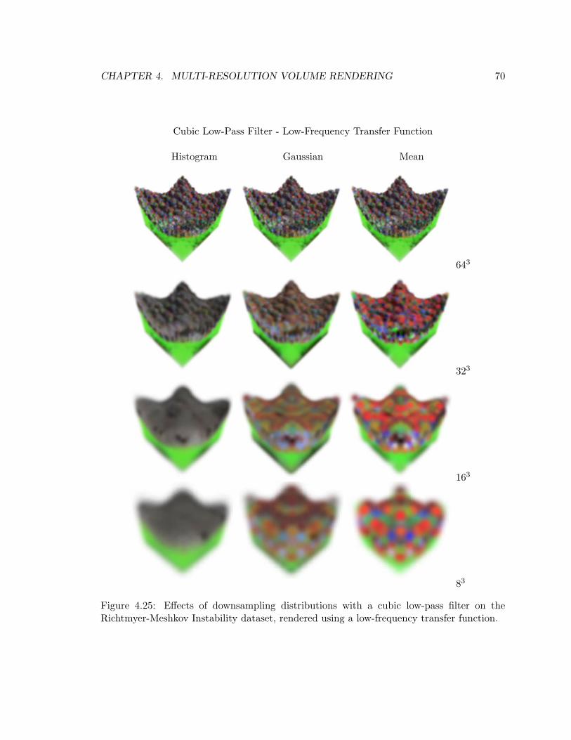
CHAPTER 4. MULTI-RESOLUTION VOLUME RENDERING 70
Cubic Low-Pass Filter - Low-Frequency Transfer Function
Histogram Gaussian Mean
643
323
163
83
Figure 4.25: Effects of downsampling distributions with a cubic low-pass filter on theRichtmyer-Meshkov Instability dataset, rendered using a low-frequency transfer function.
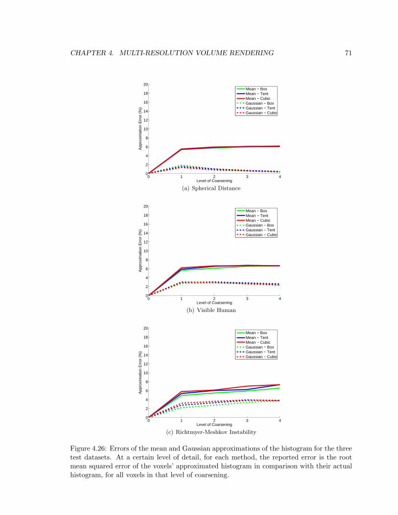
CHAPTER 4. MULTI-RESOLUTION VOLUME RENDERING 71
0 1 2 3 40
2
4
6
8
10
12
14
16
18
20
Level of Coarsening
App
roxi
mat
ion
Err
or (
%)
Mean − BoxMean − TentMean − CubicGaussian − BoxGaussian − TentGaussian − Cubic
(a) Spherical Distance
0 1 2 3 40
2
4
6
8
10
12
14
16
18
20
Level of Coarsening
App
roxi
mat
ion
Err
or (
%)
Mean − BoxMean − TentMean − CubicGaussian − BoxGaussian − TentGaussian − Cubic
(b) Visible Human
0 1 2 3 40
2
4
6
8
10
12
14
16
18
20
Level of Coarsening
App
roxi
mat
ion
Err
or (
%)
Mean − BoxMean − TentMean − CubicGaussian − BoxGaussian − TentGaussian − Cubic
(c) Richtmyer-Meshkov Instability
Figure 4.26: Errors of the mean and Gaussian approximations of the histogram for the threetest datasets. At a certain level of detail, for each method, the reported error is the rootmean squared error of the voxels’ approximated histogram in comparison with their actualhistogram, for all voxels in that level of coarsening.
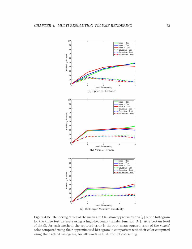
CHAPTER 4. MULTI-RESOLUTION VOLUME RENDERING 72
0 1 2 3 40
10
20
30
40
50
60
70
80
90
100
Level of Coarsening
Ren
derin
g E
rror
(%
)
Mean − BoxMean − TentMean − CubicGaussian − BoxGaussian − TentGaussian − Cubic
(a) Spherical Distance
0 1 2 3 40
10
20
30
40
50
60
70
80
90
100
Level of Coarsening
Ren
derin
g E
rror
(%
)
Mean − BoxMean − TentMean − CubicGaussian − BoxGaussian − TentGaussian − Cubic
(b) Visible Human
0 1 2 3 40
10
20
30
40
50
60
70
80
90
100
Level of Coarsening
Ren
derin
g E
rror
(%
)
Mean − BoxMean − TentMean − CubicGaussian − BoxGaussian − TentGaussian − Cubic
(c) Richtmyer-Meshkov Instability
Figure 4.27: Rendering errors of the mean and Gaussian approximations (f) of the histogramfor the three test datasets using a high-frequency transfer function (V ). At a certain levelof detail, for each method, the reported error is the root mean squared error of the voxels’color computed using their approximated histogram in comparison with their color computedusing their actual histogram, for all voxels in that level of coarsening.
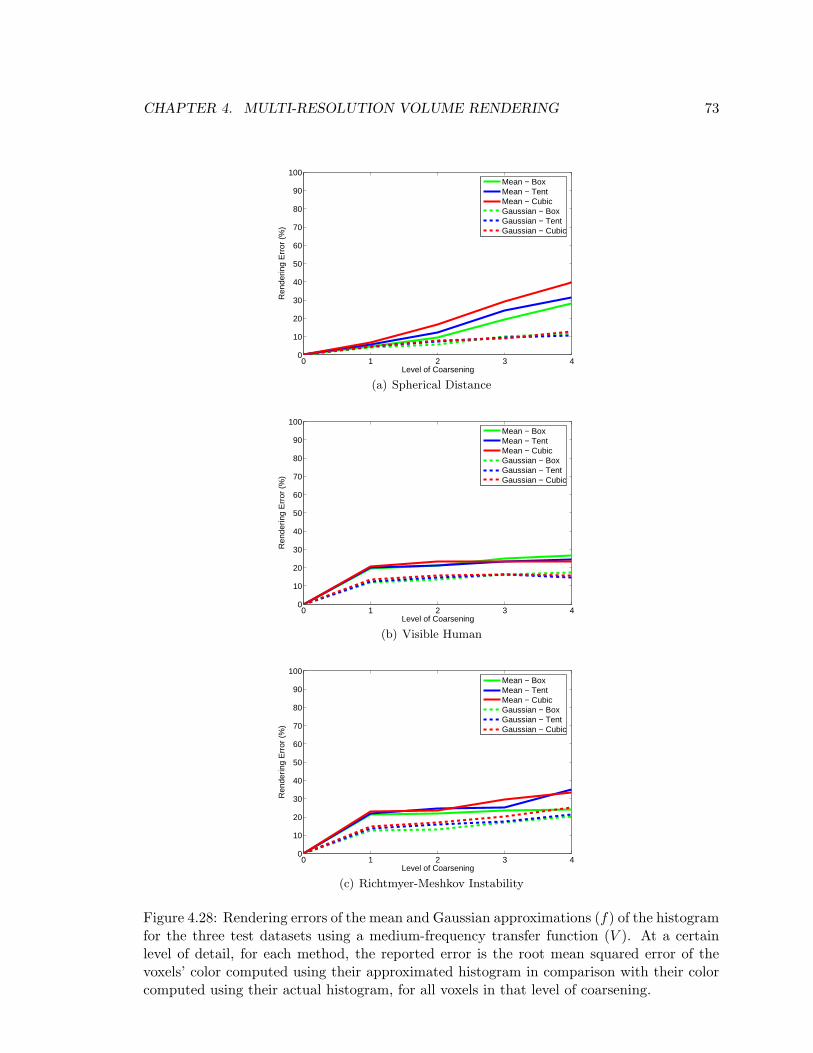
CHAPTER 4. MULTI-RESOLUTION VOLUME RENDERING 73
0 1 2 3 40
10
20
30
40
50
60
70
80
90
100
Level of Coarsening
Ren
derin
g E
rror
(%
)
Mean − BoxMean − TentMean − CubicGaussian − BoxGaussian − TentGaussian − Cubic
(a) Spherical Distance
0 1 2 3 40
10
20
30
40
50
60
70
80
90
100
Level of Coarsening
Ren
derin
g E
rror
(%
)
Mean − BoxMean − TentMean − CubicGaussian − BoxGaussian − TentGaussian − Cubic
(b) Visible Human
0 1 2 3 40
10
20
30
40
50
60
70
80
90
100
Level of Coarsening
Ren
derin
g E
rror
(%
)
Mean − BoxMean − TentMean − CubicGaussian − BoxGaussian − TentGaussian − Cubic
(c) Richtmyer-Meshkov Instability
Figure 4.28: Rendering errors of the mean and Gaussian approximations (f) of the histogramfor the three test datasets using a medium-frequency transfer function (V ). At a certainlevel of detail, for each method, the reported error is the root mean squared error of thevoxels’ color computed using their approximated histogram in comparison with their colorcomputed using their actual histogram, for all voxels in that level of coarsening.
Chapter 5
Conclusions and Future Work
In this thesis we studied the problems of large scale volumetric data visualization from the
aspect of data dimensionality and data resolution.
From the aspect of data dimensionality we studied the temporal coherence of sequential
time frames and histogram and spatial distribution of data in time-varying datasets and
proposed a new data structure called Differential Time-Histogram Table (DTHT) to take
advantage of these characteristics to efficiently load and render time-varying datasets.
In a preprocessing step, we encode the temporal coherence and histogram distribution
of the data in the DTHT data structure. Later, during the visualization step, we use this
differential information to accelerate updating data by minimizing the amount of data that
needs to be transfered from disk into main memory. To store the data in external storage and
to keep the active data in main memory, we use an octree data structure which accelerates
loading and processing data by exploiting spatial distribution.
To address high resolution data, we proposed a hybrid framework for volumetric multi-
resolution datasets to improve the quality of visualization. Using a Gaussian basis function
to approximate the data distribution at each level of detail, rather than the commonly used
mean approximation, we are able to composite color more accurately and reduce aliasing
artifacts. Our methods allow any low-pass filter to be applied to build the multi-resolution
pyramid without a-priori knowledge of the transfer function. We also use transparent iso-
surfaces to capture high-frequency sharp features and to reduce blurring in coarse resolution
renderings. In addition to the quality improvements we also proposed some techniques to
improve the interactivity of multi-resolution rendering by using a histogram code to bypass
the non-important data and by caching the partial renderings in the texture memory to do
74
CHAPTER 5. CONCLUSIONS AND FUTURE WORK 75
progressive refinement.
5.1 Future Work
The work presented for time-varying datasets was mainly focused on analyzing the statistical
characteristics of large datasets to reduce the data transfer between memory and external
storage during the visualization process. Further performance improvement would be pos-
sible by applying compression schemes for the data in leaf nodes and adding multi-level
information to the sub-levels of the data structure to enable multi-resolution renderings.
Currently the rendering time is dominating the overall time to produce an image. Image
caching, occlusion culling and parallel rendering will further drastically improve the render-
ing performance. Other future work includes applying proper modifications to DTHT in
order to enable the extraction of isosurfaces and to handle multi-modal datasets, investigat-
ing methods to change the error bounds (λ) during run time based on the user control and
the transfer funtion and methods to deal with multi-dimensional transfer functions.
For multi-resolution rendering, future work includes combining the framework with the
DTHT data structure to visualize multi-modal and time-varying datasets. We are also in-
vestigating the use of an adaptive approximation of the histogram distribution with different
function bases at different levels of detail for different datasets. To do so, we suggest to use
the ideas of Drew et al. [11] and use Singular Value Decompositon of a wavelet-compressed
histogram. Finally, we are planning on developing a parallel rendering pipeline to achieve
better performance with large datasets, and a compression scheme to benefit from locality
and spatial coherence in the data blocks to reduce the I/O and storage requirements.
Finally, a major extension to our work will be combining the idea of differential updat-
ing in DTHT with the multi-resolution framework in HYBON to create a multi-resolution
framework for visualization of large scale time-varying volumetric datasets.
Bibliography
[1] Gary Bishop, Henry Fuchs, Leonard McMillan, and Ellen J. Scher Zagier. Framelessrendering: double buffering considered harmful. In SIGGRAPH ’94: Proceedings ofthe 21st Annual Conference on Computer Graphics and Interactive Techniques, pages175–176, 1994.
[2] Imma Boada. An octree-based multiresolution hybrid framework. Future GenerationComputer Systems, 20(8):1275–1284, 2004.
[3] Ronald Bracewell. The Fourier Transform and Its Applications. McGraw-Hill, 3rdedition, 1999.
[4] Ken Brodlie, Lesley Carpenter, Rae Earnshaw, Julian Gallop, Roger Hubbold, AnneMumford, Chris Osland, and Peter Quarendon. Scientific Visualization Techniques andApplications, chapter 1. Springer-Verlag, 1992.
[5] Bradford Chamberlain, Tony DeRose, Dani Lischinski, David Salesin, and John Sny-der. Fast rendering of complex environments using a spatial hierarchy. In GI ’96:Proceedings of the Conference on Graphics Interface ’96, pages 132–141, 1996.
[6] Jatin Chhugani, Sudhir Vishwamanth, Jonathan Cohen, and Subodh Kumar. Isoslider:A system for interactive exploration of isosurfaces. In Proceedings of EurographicsVisualization Symposium 2003, pages 259–266, 304, 2003.
[7] Yi-Jen Chiang, Claudio T. Silva, and William J. Schroeder. Interactive out-of-coreisosurface extraction. In Proceedings of IEEE Visualization ’98, pages 167–174, 1998.
[8] Paolo Cignoni, Paola Marino, Claudio Montani, Enrico Puppo, and Roberto Scopigno.Speeding Up Isosurface Extraction Using Interval Trees. IEEE Transactions on Visu-alization and Computer Graphics, 3(2):158–169, 1997.
[9] Harvey Cline, William Lorensen, Siegwalt Ludke, Carl Crawford, and Bruce Teeter.Two algorithms for the reconstruction of surfaces from tomograms. Medical Physics,15(3):320–327, 1988.
[10] Scott Co, Bernd Hamann, and Kenneth I. Joy. Iso-splatting: A Point-based Alternativeto Isosurface Visualization. In Proceedings of Pacific Graphics 2003, pages 325–334,2003.
76
BIBLIOGRAPHY 77
[11] Mark S. Drew, Jie Wei, and Ze-Nian Li. Illumination–invariant color object recogni-tion via compressed chromaticity histograms of color–channel–normalized images. InICCV98, pages 533–540. IEEE, 1998.
[12] Rae A. Earnshaw and Norman Wiseman. An Introduction to Scientific Visualization,chapter 2. Springer-Verlag, 1992.
[13] Richard S. Gallagher. Span Filtering: An Optimization Scheme For Volume Visual-ization of Large Finite Element Models. In Proceedings of Visualization 1991, pages68–75. IEEE, 1991.
[14] Markus H. Gross, L. Lippert, R. Dittrich, and S. Haring. Two methods for wavelet-based volume rendering. Computers & Graphics, 21(2):237–252, 1997.
[15] Stefan Guthe and Michael Wand. Advanced techniques for high-quality multi-resolutionvolume rendering. Computers and Graphics, 28(1), 2004.
[16] Stefan Guthe, Michael Wand, Julius Gonser, and Wolfgang Straßer. Interactive ren-dering of large volume data sets. In In Proceedings of IEEE Visualization 2002, pages53–59, 2002.
[17] Editors: Charles D. Hansen and Christopher R. Johnson. The Visualization Handbook.Chapters 7, 25 – 28, 36. Elsevier Academic Press, 2005.
[18] Helwig Hauser, Lukas Mroz, Gian-Italo Bischi, and M. Eduard Groller. Two-level vol-ume rendering - fusing MIP and DVR. In Proceedings of the Conference on Visualization’00, pages 211–218, 2000.
[19] Stefan Horbelt, Martin Vetterli, and Michael Unser. High-quality wavelet splatting forvolume rendering. In Wavelet Applications Workshop, Monte Verita TI, Switzerland,September 28-October 2, 1998.
[20] Gordon Kindlmann and James W. Durkin. Semi-automatic generation of transfer func-tions for direct volume rendering. In Proceedings of the 1998 IEEE Symposium onVolume Visualization, pages 79–86, New York, NY, USA, 1998. ACM Press.
[21] Kevin Kreeger and Arie Kaufman. Hybrid volume and polygon rendering with cubehardware. In Proceedings of the ACM SIGGRAPH/EUROGRAPHICS Workshop onGraphics Hardware, pages 15–24, 1999.
[22] Kevin Kreeger and Arie Kaufman. Mixing translucent polygons with volumes. InProceedings of the Conference on Visualization ’99, pages 191–198, 1999.
[23] Phil Lacroute and Marc Levoy. Fast volume rendering using a shear-warp factorizationof the viewing transformation. In Proceedings of SIGGRAPH 94, pages 451–458, 1994.
BIBLIOGRAPHY 78
[24] Eric LaMar, Bernd Hamann, and Kenneth I. Joy. Multiresolution techniques for inter-active texture-based volume visualization. In Proceedings of the Conference on Visual-ization ’99, pages 355–361, 1999.
[25] David Laur and Pat Hanrahan. Hierarchical splatting: a progressive refinement al-gorithm for volume rendering. In SIGGRAPH ’91: Proceedings of the 18th AnnualConference on Computer Graphics and Interactive Techniques, pages 285–288, 1991.
[26] Marc Levoy. Display of surfaces from volume data. IEEE Computer Graphics andApplications, 8(3):29–37, 1988.
[27] Marc Levoy. A hybrid ray tracer for rendering polygon and volume data. IEEE Com-puter Graphics and Applications, 10(2):33–40, 1990.
[28] Marc Levoy and Ross Whitaker. Gaze-directed volume rendering. In SI3D ’90: Pro-ceedings of the 1990 Symposium on Interactive 3D Graphics, pages 217–223, 1990.
[29] Xinyue Li and Han-Wei Shen. Time-critical multiresolution volume rendering using 3Dtexture mapping hardware. In Proceedings of the 2002 IEEE Symposium on VolumeVisualization and Graphics, pages 29–36, Piscataway, NJ, USA, 2002. IEEE Press.
[30] Yarden Livnat, Han-Wei Shen, and Christopher R. Johnson. A Near Optimal IsosurfaceExtraction Algorithm Using the Span Space. IEEE Transactions on Visualization andComputer Graphics, 2(1):73–84, 1996.
[31] Patric Ljung, Claes Lundstrom, Anders Ynnerman, and Ken Museth. Transfer functionbased adaptive decompression for volume rendering of large medical data sets. InProceedings of IEEE Symposium on Visualization and Graphics 2004, pages 25–32,2004.
[32] William Lorensen and Harvey Cline. Marching cubes: A high resolution 3D surfaceconstruction algorithm. ACM SIGGRAPH Computer Graphics, 21(4):163–169, July1987.
[33] David Luebke, Benjamin Watson, Jonathan D. Cohen, Martin Reddy, and AmitabhVarshney. Level of Detail for 3D Graphics. Elsevier Science Inc., New York, NY, USA,2002.
[34] Kwan-Liu Ma and Han-Wei Shen. Compression and accelerated rendering of time-varying volume data. In Workshop on Computer Graphics and Virtual Reality, 2000International Computer Symposium, 2000.
[35] Jeff Orchard and Torsten Moller. Accelerated Splatting Using a 3D Adjacency DataStructure. In Proceedings of Graphics Interface 2001, pages 191–200, 2001.
[36] Steven Parker, Michael Parker, Yarden Livnat, Peter-Pike Sloan, Charles Hansen, andPeter Shirley. Interactive ray tracing for volume visualization. IEEE Transactions onVisualization and Computer Graphics, 5(3):238–250, 1999.
BIBLIOGRAPHY 79
[37] Steven Parker, Peter Shirley, Yarden Livnat, Charles D. Hansen, and Peter-Pike Sloan.Interactive ray tracing for isosurface rendering. In Proceedings of IEEE Visualization’98, pages 233–238, 1998.
[38] David M. Reed, Roni Yagel, Asish Law, Po-Wen Shin, and Naeem Shareef. Hardwareassisted volume rendering of unstructured grids by incremental slicing. In Proceedingsof the 1996 IEEE Symposium on Volume Visualization, pages 55–ff., Piscataway, NJ,USA, 1996. IEEE Press.
[39] Eric Reinhard, Charles D. Hansen, and Steven Parker. Interactive ray tracing of timevarying data. In Proceedings of the Fourth Eurographics Workshop on Parallel Graphicsand Visualization, pages 77–82, 2002.
[40] Larry Rosenblum, Rae A. Earnshaw, Jose Encarnacao, Hans Hagen, Arie Kaufman,Stanislav V. Klimenko, Gregory Nielson, Frits Post, and Daniel Thalmann. ScientificVisualization - Advances and Challenges, chapter 1. Academic Press, 1994.
[41] Stefan Rottger and Thomas Ertl. A two-step approach for interactive pre-integratedvolume rendering of unstructured grids. In Proceedings of the 2002 IEEE Symposiumon Volume Visualization and Graphics, pages 23–28, 2002.
[42] Han-Wei Shen. Isosurface extraction in time-varying fields using a temporal hirarchicalindex tree. In Proceedings of IEEE Visualization ’98, pages 159–166, 1998.
[43] Han-Wei Shen, Ling-Jen Chiang, and Kwan-Liu Ma. A fast volume rendering algorithmfor time-varying fields using a time-space partitioning (TSP) tree. In Proceedings ofIEEE Visualization ’99, pages 371–377, 1999.
[44] Han-Wei Shen, Charles D. Hansen, Yarden Livnat, and Christopher R. Johnson. Isosur-facing in Span Space with Utmost Efficiency (ISSUE). In Proceedings of Visualization1996, pages 287–294, 1996.
[45] Han-Wei Shen and Christopher R. Johnson. Differential volume rendering: a fast vol-ume visualization technnique for flow animation. In Proceedings of IEEE Visualization’94, pages 188–195. IEEE Computer Society Press, 1994.
[46] Peter Shirley and Allan Tuchman. A polygonal approximation to direct scalar volumerendering. Computer Graphics, 24(5):63–70, July 1990.
[47] Bong-Soo Sohn, Chandrajit Bajaj, and Vinay Siddavanahalli. Feature based volumetricvideo compression for interactive playback. In Proceedings of IEEE Symposium onVolume Visualization and Graphics 2002, pages 89–96, 2002.
[48] Philip Sutton and Charles D. Hansen. Isosurface extraction in time-varying fields usinga temporal branch-on-need tree (T-BON). In Proceedings of IEEE Visualization ’99,pages 147–153, 1999.
BIBLIOGRAPHY 80
[49] J. Edward Swan, Klaus Mueller, Torsten Moller, Naeem Shareef, Roger Crawfis, andRoni Yagel. An anti-aliasing technique for splatting. In Proceedings of the 8th Confer-ence on Visualization ’97, pages 197–ff., 1997.
[50] Takashi Totsuka and Marc Levoy. Frequency domain volume rendering. In Proceedingsof SIGGRAPH 93, pages 271–278, 1993.
[51] Ming Wan, Long Tang, Zesheng Tang, and Xinyou Li. PC-based quick algorithmfor rendering semi-transparent multi-isosurfaces of volumetric data. In Proceedings ofVisualization 1996, pages 54–61, 1996.
[52] Benjamin Watson, Neff Walker, Larry F. Hodges, and Aileen Worden. Managing levelof detail through peripheral degradation: effects on search performance with a head-mounted display. ACM Transactions on Computer-Human Interaction, 4(4):323–346,1997.
[53] Manfred Weiler, Rudiger Westermann, Chuck Hansen, Kurt Zimmermann, and ThomasErtl. Level-of-detail volume rendering via 3D textures. In Proceedings of the 2000 IEEESymposium on Volume Visualization, pages 7–13, 2000.
[54] Lee Westover. Footprint evaluation for volume rendering. In SIGGRAPH ’90: Proceed-ings of the 17th Annual Conference on Computer Graphics and Interactive Techniques,pages 367–376, 1990.
[55] Jane Wilhelms and Allen Van Gelder. Octrees for faster isosurface generation. ACMTransactions on Graphics, 11(3):201–227, July 1992.
[56] Craig M. Wittenbrink, Thomas Malzbender, and Michael E. Goss. Opacity-weightedcolor interpolation for volume sampling. In Proceedings of the 1998 IEEE Symposiumon Volume Visualization, pages 135–142, New York, NY, USA, 1998. ACM Press.
[57] Geoff Wyvill, Craig McPheeters, and Brian Wyvill. Data structure for soft objects.Visual Computer, 2:227–234, 1986.
[58] Hamid Younesy, Torsten Moller, and Hamish Carr. Hybon: Improving the qualityand interactivity of multi-resolution volume rendering using a hybrid framework. InSubmitted to IEEE Symposium on Visualization 2005, 2005.
[59] Hamid Younesy, Torsten Moller, and Hamish Carr. Visualization of time-varying vol-umetric data using differential time-histogram table. In Proceedings of Workshop onVolume Graphics 2005, pages 21–29, Stony Brook, NY, 2005.
[60] Michael Zyda. A decomposable algorithm for contour surface display generation. ACMTransactions on Graphics, 7(2):129–148, 1988.