Visualizing the Discrete Biharmonic Operator on SignedDistance Fields

Ben Jones

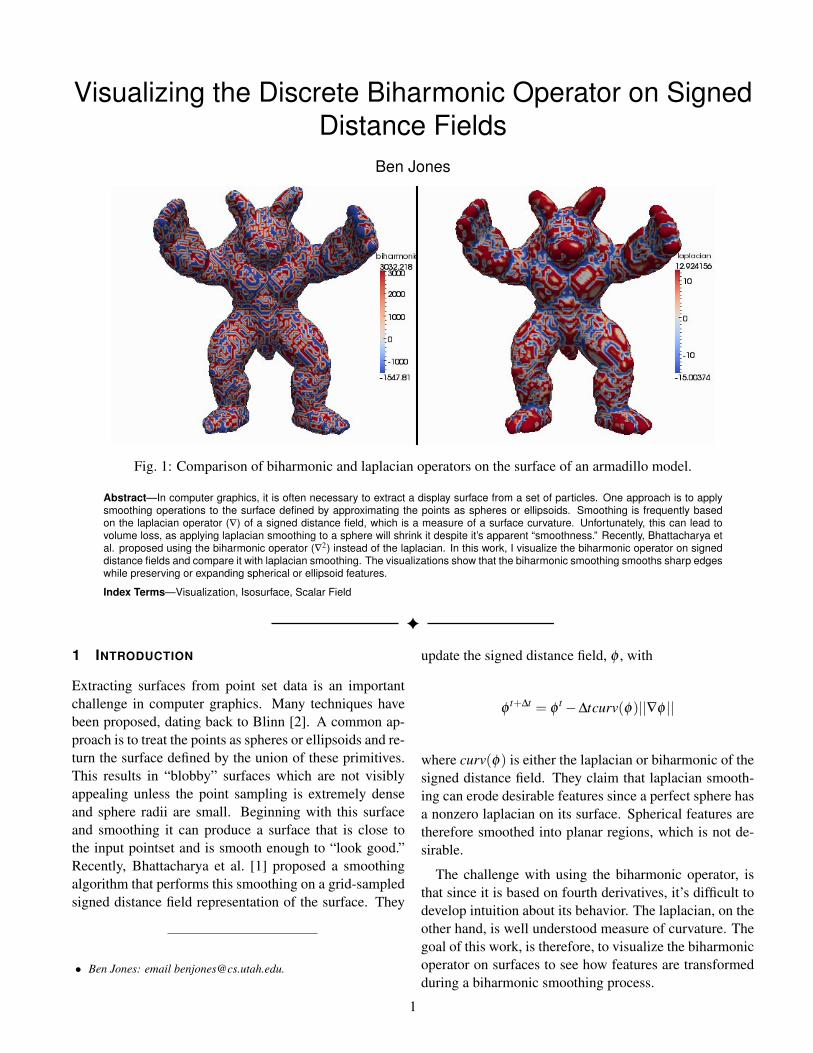
Fig. 1: Comparison of biharmonic and laplacian operators on the surface of an armadillo model.

Abstract—In computer graphics, it is often necessary to extract a display surface from a set of particles. One approach is to applysmoothing operations to the surface defined by approximating the points as spheres or ellipsoids. Smoothing is frequently basedon the laplacian operator (∇) of a signed distance field, which is a measure of a surface curvature. Unfortunately, this can lead tovolume loss, as applying laplacian smoothing to a sphere will shrink it despite it’s apparent “smoothness.” Recently, Bhattacharya etal. proposed using the biharmonic operator (∇2) instead of the laplacian. In this work, I visualize the biharmonic operator on signeddistance fields and compare it with laplacian smoothing. The visualizations show that the biharmonic smoothing smooths sharp edgeswhile preserving or expanding spherical or ellipsoid features.

Index Terms—Visualization, Isosurface, Scalar Field

1 INTRODUCTION

Extracting surfaces from point set data is an importantchallenge in computer graphics. Many techniques havebeen proposed, dating back to Blinn [2]. A common ap-proach is to treat the points as spheres or ellipsoids and re-turn the surface defined by the union of these primitives.This results in “blobby” surfaces which are not visiblyappealing unless the point sampling is extremely denseand sphere radii are small. Beginning with this surfaceand smoothing it can produce a surface that is close tothe input pointset and is smooth enough to “look good.”Recently, Bhattacharya et al. [1] proposed a smoothingalgorithm that performs this smoothing on a grid-sampledsigned distance field representation of the surface. They

• Ben Jones: email benjones@cs.utah.edu.

update the signed distance field, φ , with

φt+∆t = φ

t −∆tcurv(φ)||∇φ ||

where curv(φ) is either the laplacian or biharmonic of thesigned distance field. They claim that laplacian smooth-ing can erode desirable features since a perfect sphere hasa nonzero laplacian on its surface. Spherical features aretherefore smoothed into planar regions, which is not de-sirable.

The challenge with using the biharmonic operator, isthat since it is based on fourth derivatives, it’s difficult todevelop intuition about its behavior. The laplacian, on theother hand, is well understood measure of curvature. Thegoal of this work, is therefore, to visualize the biharmonicoperator on surfaces to see how features are transformedduring a biharmonic smoothing process.

1

Fig. 2: Comparison of biharmonic and laplacian operatorson a sphere. Biharmonic value is 0 across the surface,laplacian value is a positive constant.

2 APPROACH

To gain insight on the biharmonic operator, I chose torender example surfaces with a color map, correspond-ing the biharmonic value. The surfaces were generatedfrom two sources. First, for simple geometry, such ascubes and spheres, the signed distance field can be con-structed analytically. For more complicated examples, thecode from Bhattacharya et al. [1] was used to convert aset of spheres or ellipsoids into a signed distance field.In both cases, derivatives were computed using a 3-pointfinite difference stencil in each dimension. The laplaciancomputed as the sum of the finite differences of the signeddistance field, and the biharmonic analogously using thesame stencils on the laplacian field.

To render the surfaces, I used ParaView [3] visualiza-tion software, which is based on the VTK toolkit. Therendered surface is the 0-levelset of the signed distancefield, which was extracted by contouring. The color ismapped based on interpolated values of the biharmonicoperator.

In order to see how the biharmonic and laplacian fieldschanged during the smoothing passes described by Bhat-tacharya et al. [1], I generated animated sequences duringthe process. I used ParaView to generate animations fromthe three scalar fields at each timestep.

3 RESULTS

In all the example below, blue colors indicate negativevalues, and red shades indicate positive values. Duringsmoothing, blue regions would be pushed outward, andred regions would shrink inward. Animated versions ofmany examples are included in the accompanying video.

3.1 Sphere

To confirm that laplacian smoothing applied to a spherewill shrink it, while biharmonic smoothing will not, myfirst example is of a sphere, shown in fig. 2. As predicted,

Fig. 3: Comparison of biharmonic and laplacian operatorson an ellipsoid before smoothing.

Fig. 4: Comparison of biharmonic and laplacian operatorson an ellipsoid after biharmonic smoothing.

the laplacian is a positive constant over the entire surface,and would therefore be shrunk by a laplacian smoothingpass. The biharmonic field is zero over the entire surface,and would therefore be preserved.

3.2 Ellipsoid

Ellipsoids are also used to initialize a bounding surfaceof a point set when there is anisotropy. Examples of thisinclude stretching based on velocity or neighborhood in-formation. Figure 3 and fig. 4 show a comparison betweenbiharmonic and laplacian operators on an ellipsoid beforeand after 20 passes of biharmonic smoothing. Since theellipsoid is convex, the laplacian value is positive every-where on the surface. The biharmonic operator, however,changes sign near the center of the major axis of the ellip-soid. It appears that pure biharmonic smoothing wouldshrink the center of the ellipsoid and expand the ends.Without constraints, I hypothesize that it would result in2 distinct spheres at equilibrium.

3.3 Cube

A smoothing operator should smooth away sharp edgesin order to be useful. To ensure that the biharmonic op-erator does so, I analyzed it’s effect on a cube. As ex-pected, the flat sides have a zero biharmonic value mod-ulo errors in the finite difference approximations. With

2

Fig. 5: Biharmonic operator applied to cube. Flat surfaceswill be preserved, but edges and corners will be pushedinward during smoothing.

the stencil width of the edges, however, the values be-come positive and increasingly large. Sharp corners havethe largest values. When smoothing, the edges on thecube would be move inward, rounding them, resulting ina smoother surface as desired. The magnitude of the op-erator at sharp edges and corners is much greater than themagnitude seen on the sphere and ellipsoid examples, in-dicating that they will be smoothed much more aggres-sively than curved patches.

3.4 Armadillo

The final example I analyzed is a model representative ofactual use of particle skinning algorithms. It is a surfacecontaining a wide range of curvatures and features. Fig-ure 6 shows a comparison of the laplacian and biharmonicoperators before and after smoothing. The biharmonic op-erator tends to preserve appendages better than the lapla-cian operator, as can be seen in the close up of the hand infig. 7.

CONCLUSIONS

The visualizations generated demonstrate the differencebetween the biharmonic and laplacian operators on signeddistance fields. In general, laplacian smoothing tends toshrink extruding features, while biharmonic smoothingtends to expand the features, but shrink the regions con-necting them to other objects.

Improvements

The biggest problem with the approach I used is that thesmoothing algorithm I used from Bhattacharya et al. [1] isa constrained optimization. At each step, the signed dis-tance field is bounded by the original point set. Becauseof that, it’s difficult to examine how the biharmonic oper-ator is affecting the surfaces versus how the bounds affectit. For example, the chest of the armadillo does not have

Fig. 7: Close up of the armadillo’s hand. Biharmonicsmoothing would inflate the fingers, while laplaciansmoothing would shrink them.

a zero biharmonic value, yet the constraints keep it fromchanging significantly during the optimization. If I wereto re-do the project, I would remove the constraints andexamine how the surfaces evolve unconstrained, which Ibelieve would provide a better comparison between thetwo operators.

ACKNOWLEDGMENTS

This work made use of code provided by Haimasree Bhat-tacharya and Yue Gao and Adam Bargteil.

REFERENCES

[1] H. Bhattacharya, Y. Gao, and A. W. Bargteil. A level-set method for skinning animated particle data. InProceedings of the ACM SIGGRAPH/EurographicsSymposium on Computer Animation, Aug 2011.

[2] J. Blinn. A generalization of algebraic surface draw-ing. ACM Transactions on Graphics (TOG), 1(3):235–256, 1982.

[3] Kitware. Paraview, 2002-2011. www.paraview.org.

3

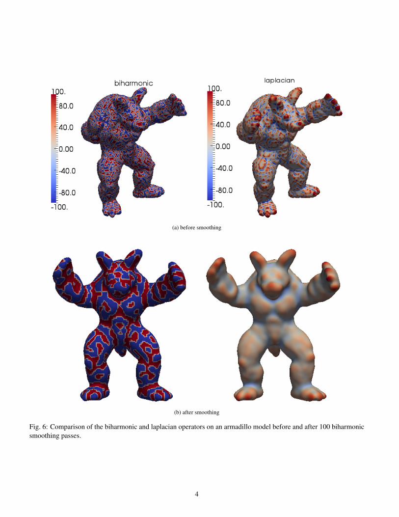
(a) before smoothing

(b) after smoothing

Fig. 6: Comparison of the biharmonic and laplacian operators on an armadillo model before and after 100 biharmonicsmoothing passes.

4