Potential Vortex Transient Analysis and Experiment John R. Cipolla

Email: john@aerorocket.com

709 West Homeway Loop, Citrus Springs FL 34434

Abstract A series of experiments and hydrodynamic analyses has been conducted to resolve the

paradox that a viscous-flow distribution between concentric cylinders can be identical to

a potential vortex (inviscid-flow) distribution at steady state. Where a potential vortex or

tornado can be described as the flow around and through a drain hole at the bottom of a

large container. As an approximation to this phenomenon, an experimental device to

simulate a three dimensional potential vortex was fabricated that used a rapidly rotating

central cylinder or rotating core located on the axis of a cylindrical basin filled with

water. The fluid surface shape and velocity profile of an artificially generated potential

vortex or free vortex was experimentally measured and compared with hydrodynamic

models to define the viscid and inviscid nature of the potential vortex flow. A new

program called VORTEX based on a finite difference solution of the Navier-Stokes

equations was developed to determine the transient velocity profile and transient free

surface shape of the potential vortex for comparison with experiment. From these

experiments it is proposed the paradox is resolved because energy-momentum is

conserved in a potential vortex under steady state conditions. This work can be applied to

the measurement of the potential vortex flow generated by aircraft wing tips, interior flow

of aircraft jet engines, rocket motor propellant tanks and natural phenomena like

tornadoes, hurricanes and General Relativity.

Copyright © 2014 John Cipolla/AeroRocket.com

I. Introduction An experimental device to simulate a three dimensional potential vortex was fabricated

that used a rapidly rotating central cylinder or core located on the axis of a cylindrical

basin filled with water. One purpose of this paper is to document the difficulty of

fabricating an experiment to generate a “standing” potential vortex without the inherent

mechanical vibrations that can cause turbulence in the flow field and make physical

measurement difficult. For even a well-designed apparatus, physical measurement of the

potential vortex surface is extremely difficult because of the constant wave action caused

by turbulence and flow separation. At first it was envisioned that a probe extended onto

the surface might be used to indicate surface location relative to a datum surface like the

still height,  𝑧!!. Where, the still height is the fluid surface location in the basin when the

rotating core is stationary. Instead, for comparison of theoretical and experimental fluid

surface shapes and velocity profiles the following approaches were used. First, theoretical

surface shapes are superimposed on photographs of the corresponding observed surface

shapes for a graphical approach to data reduction. Second, physical measurement of fluid

velocity was only practical in the center of the basin where turbulence effects were not

significant. Physical measurement of free surface velocity in the central location of the

basin was achieved by using video that recorded the motion of a small Styrofoam ball

placed in the vortex to determine orbital velocity of the fluid carrying the ball. Also, this

paper proves the velocity profile equation for a potential vortex where the outer cylinder

is located infinitely far away is not sufficient to model the case of fluid flow between two

concentric cylinders. Instead, an analysis where the inner cylinder rotates and the outer

cylinder is stationary is required to accurately model the velocity profile. Finally, an

attempt is made to explain why the transient flow between two concentric cylinders used

to generate a potential vortex has a steady state viscous-flow velocity distribution that is

identical to inviscid potential-flow.

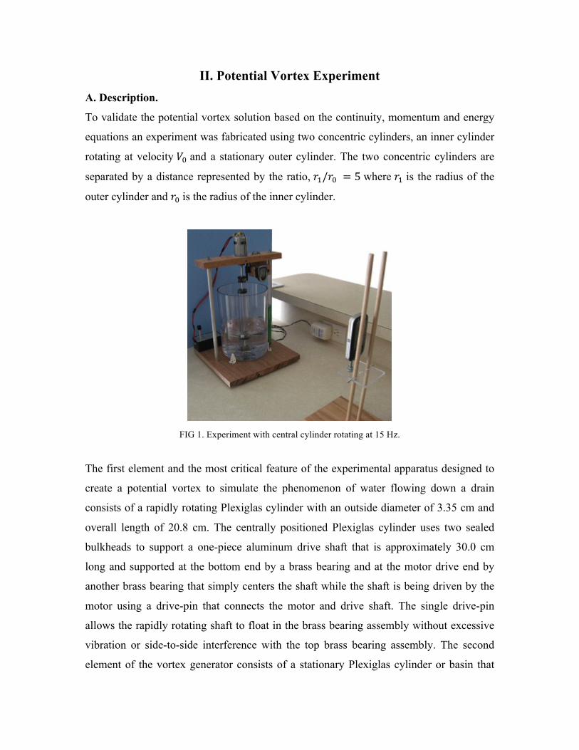
II. Potential Vortex Experiment A. Description.

To validate the potential vortex solution based on the continuity, momentum and energy

equations an experiment was fabricated using two concentric cylinders, an inner cylinder

rotating at velocity 𝑉! and a stationary outer cylinder. The two concentric cylinders are

separated by a distance represented by the ratio, 𝑟!/𝑟!  = 5 where 𝑟! is the radius of the

outer cylinder and 𝑟!  is the radius of the inner cylinder.

FIG 1. Experiment with central cylinder rotating at 15 Hz.

The first element and the most critical feature of the experimental apparatus designed to

create a potential vortex to simulate the phenomenon of water flowing down a drain

consists of a rapidly rotating Plexiglas cylinder with an outside diameter of 3.35 cm and

overall length of 20.8 cm. The centrally positioned Plexiglas cylinder uses two sealed

bulkheads to support a one-piece aluminum drive shaft that is approximately 30.0 cm

long and supported at the bottom end by a brass bearing and at the motor drive end by

another brass bearing that simply centers the shaft while the shaft is being driven by the

motor using a drive-pin that connects the motor and drive shaft. The single drive-pin

allows the rapidly rotating shaft to float in the brass bearing assembly without excessive

vibration or side-to-side interference with the top brass bearing assembly. The second

element of the vortex generator consists of a stationary Plexiglas cylinder or basin that

forms the outer boundary of the flow field which has an inside diameter of 16.4 cm and

overall height of 23.6 cm. A DC motor speed control and small DC motor form the third

element of the vortex generator. Rotation speed of 2 to 30 cycles per second (Hz) is

possible using the system depicted in Figure 1. Finally, the rotation rate measurement

system illustrated in Figure 1 forms the forth and final element of the vortex generator.

The measurement system consists of a standard bicycle speed measurement computer,

magnetic probe and a drum attached to the shaft that holds the sensor magnet. As

displayed in Figure 1 the velocity of the rotating drum is 4.6 km per hour, which means

the rotating drum holding the sensor magnet has a rotation rate of 15 Hz. This is the

rotation rate of the shaft and the rotating cylinder when driven by the DC electric motor.

B. Experimental and theoretical free surface deflection compared

A potential vortex or tornado is often approximated by the flow around a drain hole at the

bottom of a container. As an approximation to this phenomenon and to generate a

standing vortex, an experimental device to simulate a three dimensional potential vortex

has been fabricated that uses a rapidly rotating central cylinder located on the axis of a

cylindrical basin filled with water. A rotating cylindrical core forms the inner boundary

around which the potential vortex is created while maintaining an approximately non-

viscous or inviscid boundary condition on the outer boundary of the flow. The rotating

inner boundary’s non-slip or viscous boundary drags circumferential layers of fluid that

generate the potential vortex. The rotating inner core of the experiment represents the

rotating inner boundary of the potential vortex. The circumferential velocity profile for

the potential vortex at steady state is:

𝑢! =  !!    !!  !

(1)

Where r is measured from the center of the system, 𝑉! is the rotation velocity at the

surface of the inner vortex core and 𝑟! represents the radius of the inner rotating cylinder.

Velocity in the radial direction, 𝑢! is zero and 𝑟!  represents the outer radius of the

stationary cylindrical basin. Figure 2 displays the geometry for the free surface and

velocity profile analysis and provides nomenclature for the experiment. During initial

startup, viscous interactions between subsequent layers of fluid generate a time varying

velocity profile and free surface deflection. The transient phase of flow cannot be

considered irrotational. However, at steady state the velocity profile and free surface

deflection of the resulting fluid flow can be approximated by an irrotational solution

based on the viscous Navier Stokes equations in the circumferential, radial, and vertical

(𝜃, r, z) directions when the proper boundary conditions are imposed. The Navier Stokes

solution for the potential vortex generates a velocity distribution that is incompressible

where ∇   ∙  𝑽 = 𝟎 and irrotational where ∇  ×  𝑽 = 𝟎 throughout the flow field at steady

state. The final solution for the steady state potential vortex is the Bernoulli equation, that

holds everywhere in the flow including the free surface where p = 𝑝!"# and forms a

series of constant-pressure surfaces having the form of a second-order hyperboloid, that

is, z varies inversely with 𝑟!. Where the Bernoulli equation for p is expressed as1.

𝑝 =  !  !!

!  !!+  𝜌  𝑔  𝑧 = 𝐶 (2)

FIG. 2. Free body diagram for an object on the free surface of a potential vortex.

Where 𝐾 =  𝑉!  𝑟! and the constant, C must be determined to compute the shape of the

fluid surface at p = 𝑝!"#  which represents the free surface of the potential vortex

described in Figure 2. After solving for fluid height, z using the Bernoulli equation, then

applying the pressure boundary condition 𝑝 = 𝑝!"#  on the free surface to determine the

constant C, a free surface of constant pressure 𝑝!"#  has the following shape as a function

of r from the center of the rotating cylinder.

𝑧  !!!! =  𝐶! −  !!!!!!

!  !  !!  . Where 𝐶! =  𝑧! +

!!!

!!   (3)

Then, Eqn. 3 can be rearranged with one unknown, 𝑧! remaining.

𝑧 =  𝑧! +!!!

!!  (1− !!!

!!) (4)

Where, 𝑧!  is the vertical intersection of the fluid free surface with the central rotating

cylinder from the bottom of the basin illustrated in Figure 2. The unknown distance is

determined by solving the following fluid volume equation.

𝑉𝑂𝐿!"!#$ = 𝑉𝑂𝐿 + 𝑉𝑂𝐿! (5)

Where 𝑉𝑂𝐿!"!#$ is the total, still or motionless volume of fluid when the initial depth of

the fluid in the basin is 𝑧!!, 𝑉𝑂𝐿 is the volume of fluid below the plane defined by 𝑧 = 𝑧!

and the bottom of the basin and 𝑉𝑂𝐿!  is the volume of fluid determined by integrating

between the free surface (Eqn. 4) defined by 𝑝 = 𝑝!"#  and plane 𝑧 = 𝑧!. The following

three equations define the three fluid volumes required to determine the unknown.

𝑉𝑂𝐿!"!#$ = 𝜋 𝑟!! − 𝑟!! 𝑧!! (6)

𝑉𝑂𝐿 =  𝜋 𝑟!! − 𝑟!! 𝑧! (7)

𝑉𝑂𝐿! = !!!!

!!𝑟!! − 𝑟!! − 2𝑟!!ln

!!!!

(8)

Finally, after some algebra the resulting equation for the vertical intersection of the fluid

free surface with the central rotating cylinder from the bottom of the basin becomes.

𝑧!=𝑧!! −!!!

!!  1− !!!!

!!!!!!!ln !!

!! (9)

The potential flow equations represented by Eqn. 4 and Eqn. 9 are used to produce the

surface deflection curves superimposed on the experimental shapes depicted in Figures 3-

4 for rotation rates of 10 Hz and 15 Hz respectively. Results in Figure 3 validated the

experimental free surface deflection by superimposing theoretical surface deflection on a

photographic image of the actual surface deflection. Table I displays potential vortex

surface measurement results compared to theoretical inviscid and irrotational potential

vortex flow. Measurement of the potential vortex surface was extremely difficult because

of the constant wave action superimposed on the surface. At first it was envisioned that a

probe extended onto the surface might be used to indicate surface location relative to a

datum surface like the still height,  𝑧!!. The still height is the fluid surface location in the

basin when the central core is stationary. Instead, for comparison of theoretical and

experimental fluid surface deflection the following approach was used.

FIG. 3. Experimental free surface and theoretical free surface compared. (a) 10 Hz, (b) 15 Hz

FIG. 4. Experimental (red dots) verses theoretical (blue line) potential vortex surfaces. (a) 10 Hz, (b) 15 Hz

As illustrated in Figure 3a and Figure 3b theoretical potential vortex surface shapes are

superimposed on photographs of the corresponding experimental surface shapes for a

graphical approach to data reduction. When generating the composite images displayed in

Figures 3-4 care was taken to properly scale the curves using marks on the theoretical

plots and marks on the images of the fluid vortex rotating at 10 Hz and 15 Hz. In Figures

3-4 please note that agreement between experimental and theoretical surface shapes is

best for the 10 Hz case because turbulence effects are less than for the corresponding 15

Hz case. In both cases agreement between theoretical and experimental results were

worse near the rotating cylinder due to intense turbulence and flow separation. However,

agreement between experimental and theoretical surface shapes based on Eqn. 4 is good.

TABLE I. Summary of theoretical verses measured potential vortex surface deflection.

𝜔!

Hz  

𝑧!!(cm)

Still height

From bottom

𝑧(cm)

𝑟 = 3.5  𝑐𝑚

Equation 4

𝑧(cm)

𝑟 = 3.5  𝑐𝑚

Measured

𝑧!(𝑐𝑚)

𝑟 = 𝑟!

Equation 4

𝑧!(cm)

𝑟 = 𝑟!

Measured

10 8.26 7.77 7.2 (-7.33%) 8.80 8.4 (-4.54%)

15 8.26 7.17 6.7 (-6.55%) 9.48 8.7 (-8.23%)

Free surface shape measurements are displayed in Table I when the central cylinder

rotates at 10 Hz and 15 Hz. The values displayed in the second, third and fifth columns

are theoretical potential vortex deflections measured from the bottom of the basin where

𝑧 = 0 . As noted by these measurements good agreement between theoretical and

experimental free surface deflection is achieved in the central region of the potential

vortex because turbulence effects are minimal. In contrast, the region near the rotating

core departs from potential vortex theory due to intense turbulence caused by flow

separation from the surface of the rotating core.

C. Experimental and theoretical free surface orbital velocity compared

Potential vortex surface velocity is determined by measuring the time it takes a red-

spotted Styrofoam ball to orbit the potential vortex by using a video camera to document

the orbital motion on the surface of the potential vortex. Physical measurement of free

surface fluid velocity was only practical in the center of the basin where turbulence

effects were not significant. Measurement of free surface velocity was achieved by using

video that recorded the motion of a Styrofoam ball placed in the vortex to determine

orbital velocity of the fluid carrying the ball knowing the radius and orbital period.

The following discussion describes how the orbital velocity of an object on the free

surface relates to surface velocity of a potential vortex. The local surface shape of a

potential vortex that supports an orbiting object, allows an object to orbit at a velocity

that is a function of core rotation rate, radius to the object on the free surface and free

surface curvature or inclination. The velocity of an object on the free surface is due to the

dynamic equilibrium between object inertia, 𝑚𝑎! object weight, W and the local surface

deformation or curvature of the free surface. Specifically, the local slope of the vortex

free surface under an orbiting object allows the object to be in dynamic equilibrium under

the action of its own weight, W normal force, N exerted by the surface and the inertia

vector, −𝑚𝑎! directed opposite to 𝑎!.

FIG. 5. Free surface rotation velocity experiment

FIG. 6. Free surface rotation velocity movie. Requires QuickTime.

Where, the centripetal acceleration, 𝑎! is directed away from the center of the circular

path of the object when the object is in orbit around the rotating core of the vortex. The

local deformation or curvature of the vortex free surface causes the object to orbit in the

direction of rotation of the inner surface. Therefore, the velocity of the object orbiting at a

point on the free surface is purely a function of the physical characteristics of the inner

surface having some angular rate of rotation and radius. This analysis implies local

curvature of a potential vortex allows the object to orbit on the surface and objects placed

on the surface move at the same orbital velocity as the potential vortex in those locations.

Also, orbital velocity of an object on the potential vortex is derivable from the curvature

or slope of the free surface and is identical to the potential vortex velocity specified by

Eqn. 1. For this experiment, free surface velocity was validated using video that recorded

the motion of a small Styrofoam ball placed in the vortex to determine orbital velocity of

the fluid carrying the ball. Then, after selecting a segment of the video when the ball is at

the center of the basin an accurate fluid surface rotational velocity can be calculated by

measuring the time of rotation from the video. The data displayed in Figure 7a and Figure

7b indicates the presence of the stationary outer cylinder significantly affects the velocity

profile correlation between theory and experiment. A solution of the continuity and

momentum equations verified the cylinder separation has a profound effect on the

velocity profile as illustrated in Figures 7a and Figure 7b but correlation between

experiment and theory has been achieved to within engineering accuracy.

FIG. 7. Potential vortex velocity profile compared to theoretical prediction. (a) 10 Hz, (b) 15 Hz

Figure 7a and Figure 7b present results of the experiment where No outer cylinder

represents the case where there is no outer cylinder and Stationary outer cylinder

represents the case where the outer cylinder is a finite distance away. For the 10 Hz

rotation rate the orbital radius was determined from the video to be 5.4 cm from the

center of the basin and the time to orbit the basin was 1.8 seconds. Additionally, for the

15 Hz rotation rate the orbital radius was also determined to be 5.4 cm from the center of

the basin and the time to orbit the basin was 1.3 seconds. The surface velocity results

displayed in Table II are within engineering accuracy indicating the analysis for the

Stationary outer cylinder where the outer cylinder is a finite distance away is valid. In

addition, only when the outer cylinder is located infinitely far away does the velocity

profile result in true irrotational potential vortex flow as depicted by the curve labeled No

outer cylinder (Eqn. 1). This experiment generated potential vortex flow that is nearly

irrotational because the data labeled Measured compares favorably to the theoretical

analysis represented by the curve labeled, Stationary outer cylinder (Eqn. 23) for the

cylinder separation used in this experiment. However, designing an experiment that

generates true irrotational potential vortex flow would require a 𝑟!/𝑟! ratio so large that

the cost would be prohibitive. Therefore, for the generation of a nearly irrotational

potential vortex the separation ratio 𝑟!/𝑟! = 5  used in this experiment is considered

sufficient12. However, the objective here was to design an experiment that is capable of

producing a fluid flow having the theoretical properties of a potential vortex in the region

away from the concentric walls.

TABLE II. Summary of theoretical verses measured potential vortex surface velocity at 𝑅!"#$% .

𝜔!  

(Hz)

𝑉!

(cm/sec)

𝑟!

(cm)

𝑅!"#$%

(cm)

𝑇!"#$%

(sec)

𝑢!_!"#$%𝑉!

Eqn. 1

𝑢!_!"#$%𝑉!

Eqn. 23

𝑢!_!"#$%𝑉!

Measured

10 105.2 1.675 5.4 1.8 0.31 0.183 0.179 (-2.2%)

15 157.9 1.675 5.4 1.3 0.31 0.183 0.165 (-9.8%)

III. Verifying that potential vortex flow is irrotational Potential vortex irrotationality was determined by observing the axial rotation rate of a

red-spotted ball while orbiting the potential vortex. To determine the sense of rotation of

a point on the vortex free surface a 2.22 cm diameter red-spotted ball was inserted on the

surface when the flow was fully developed at steady state. The orbiting ball experiment,

as illustrated by the QuickTime movie in Figure 8, indicates potential vortex flow is

irrotational when the vortex is fully developed at steady state because the ball does not

rotate around its vertical axis relative to the surface of the potential vortex. However,

when the central core is turned off the flow is rotational because the ball rotates around

its vertical axis during the coast phase to zero motion.

FIG. 8. Free surface velocity and ball-spin movie. Requires QuickTime.

The following analysis illustrates that for potential vortex flow or the flow outside a

rotating central core, the flow is irrotational because vorticity, 𝜔! is zero. This

experiment illustrates the flow is irrotational because the red spotted ball moves as a solid

body in the central region of the basin. The vorticity of potential vortex flow is computed

as follows. Where, the angular motion of a particle is defined as  𝜔! =!!∇  ×  𝑽.

𝑢! =!!!!!

(10)

𝑉! = 𝑟!𝜔. Therefore 𝑢! =!!!!!

(11)

𝜔! =!!!(!!!)!"

- !!!!!!"

(12)

𝜔! = 0 (13)

In addition, for a solid vortex or the region within a rotating central core, the fluid flow is

rotational because vorticity is non-zero. The vorticity of solid vortex flow is computed as

follows. Where, the angular motion of a particle is defined as  𝜔! =!!∇  ×  𝑽.

𝑢! = 𝑟𝜔 (14)

𝜔! =!!!(!!!)!"

- !!!!!!"

(15)

𝜔! = 2𝜔 (16)

By definition,  𝜔!  is defined as the net angular rotation that measures the localized spin of

a fluid particle along its path of travel. As a consequence if 𝜔! = 0 the flow is irrotational

and the vorticity, ∇  ×  𝑽 must be zero. However, if the flow is rotational then the vorticity

∇  ×  𝑽 must be non-zero for a fluid particle along its path of travel. This definition

indicates the free surface carrying the red spotted ball at the central point where the

rotation was observed is irrotational and frictionless for potential vortex motion.

IV. General case of flow between two concentric cylinders The following is a general derivation of the velocity profile between two concentric

cylinders where viscous effects have been neglected. The continuity and momentum

equations and the associated boundary conditions for the flow field between rotating

concentric cylinders3, 4 is presented for the case of a central rotational solid vortex and

outer irrotational potential vortex. These equations prove that a rotational solid vortex is

at the heart of every potential vortex, which follows naturally from fluid mechanics.

Continuity: !"!"= 0 (17)

r momentum:

!"!"= !!!

!

! (18)

𝜃  momentum: !!!!!!!

+ !!"

!!!

= 0 (19)

The fluid boundary conditions at the inner cylinder, 𝑟!  and the outer cylinder, 𝑟!  can be

specified as the following.

𝑟 = 𝑟!: 𝑢! = 𝑟!𝜔!,𝑝 = 𝑝! and at 𝑟 = 𝑟!: 𝑢! = 𝑟!𝜔! (20)

The solution for 𝑢! can be put in dimensionless form as the following.

!!!!!!

=  ! !!

!!!/  !!!!!!!!!!

!!!!!− 1 −

!! !

!!!!!

!!!

!!!!− 1 (21)

The velocity profile in the limit where the inner cylinder vanishes (𝑟! = 0) and the outer

cylinder rotates at rotation rate, 𝜔! represents the case of rotational solid-body rotation.  

𝑢! = 𝜔!𝑟 (22)

Finally, the following equation is used to generate the red-dashed curve in Figures 7a and

Figure 7b labeled Stationary outer cylinder, where the data point Measured is the result

of this experiment. This equation generates the velocity profile in the 𝜃 direction when

the inner cylinder rotates and the outer cylinder is stationary. The following equation

provided the best fit with measured surface velocity displayed in Figure 7.

𝑢! =  !!!!

!!!/  !!!!!!!!

!!!− !

!! (23)

In the limit as the outer cylinder is placed infinitely far away 𝑟! → ∞  the flow becomes

a true potential vortex of the familiar form presented previously.

𝑢! =!!!!!!

(24)

In terms of rotating inner cylinder strength, K the velocity profile for a potential vortex is

the following. Where 𝐾 = 𝑉!𝑟!.

𝑢! =!! (25)

V. Transient velocity solution4, 6, 8 using the Navier-Stokes equation Steady state flow between two concentric cylinders is inviscid and irrotational when the

inner cylinder rotates and the outer cylinder is stationary. However, during the transient

or startup phase the flow is viscous and governed by the Navier-Stokes equations in

cylindrical coordinates where 𝑢! ,𝑢! and 𝑢! are flow velocities in the 𝑟,𝜃 and 𝑧 directions

respectively. To prove the paradox that transient free vortex flow is viscous and the

steady state solution is inviscid and irrotational the following analysis using a finite

difference solution of the Navier-Stokes equations in cylindrical coordinates is presented.

For this application a CFD computer code called VORTEX was developed to model the

general response of transient viscous flow between concentric cylinders. For one-

dimensional viscous flow the velocity is only a function of 𝜃, 𝑡 and viscosity. Therefore,

the Navier-Stokes equations reduce to the following single equation.

𝜇 !!!!!!!

+ !!!!!!"− !!

!!= 𝜌 !!!

!" (26)

After central differencing Eqn. 26 the resulting time marching finite difference equation

to determine velocity distribution as a function of time takes the following form.

𝑢!!!! = 𝑢!!+CFL 1+ !!!!!

𝑢!!!! − 2+ ∆!!!

!  𝑢!! + 1− ∆!

!!𝑢!!!!                  (27)

Where the non-dimensional time and stability criterion in Eqn. 27 is defined as follows.

CFL = !!

∆!∆! ! (28)

For these equations 𝜇 represents the coefficient of viscosity, 𝜌 is the fluid density, ∆𝑡 is

the time increment and ∆𝑟 is the special increment in the radial direction of fluid flow.

Table III summarizes numerical and stability criteria for the VORTEX finite difference

numerical analysis using Eqn. 27 and Eqn. 28. Where, adjusted viscosity allows the

transient solution to reach steady state (𝑇!!) in 2.46 minutes compared to 2.7 minutes for

the experimentally observed steady state response of the potential vortex free surface.

 TABLE III. Numerical analysis input parameters and kinematic viscosity.

CFL 𝑟!(cm) 𝑟!(cm)

𝑧!!  (cm) N 𝜈 =

𝜇𝜌    

𝑚!

𝑠𝑒𝑐   𝑇!! (Minutes)

0.5 1.675 8.2 8.26 50 1.05E-6 (water) 2.7 (measured)

0.5 1.675 8.2 8.26 50 1.05E-5 (adjusted) 2.46 (analysis)

Boundary conditions on the interior and exterior of the flow field determine if the

solution represents the case where the outer stationary cylinder is located infinitely far

away as represented by Eqn. 24 or if the outer cylinder is located a finite distance away as

represented by Eqn. 23. The boundary conditions on the interior and exterior of the flow

are represented by the following relationships. First, for when the outer cylinder is

located infinitely far away (Eqn. 24).

𝑢!!!! = 𝑢!!!!!! (29)

Then, for when the outer cylinder is located a finite distance away (Eqn. 23).

𝑢!!!! = 0 (30)

For both cases the velocity boundary condition on the inner cylinder is as usual.

𝑢!!!! = 𝑉!                                                                                                                            (31)

The finite difference solution of the Navier-Stokes equation predicts the flow between

two concentric cylinders is viscous and rotational during the transient or time-dependent

phase. However, at steady state the results are exactly equivalent to the potential flow

equations represented by Eqn. 23 and Eqn. 24 where the flow is inviscid.

FIG. 9. Velocity profile. (a) Infinitely far apart (3000 iterations). (b) Finite distance apart (1750 iterations).

Solution of the Navier-Stokes equation (Eqn. 27) using the finite difference approach is

illustrated in Figure 9a and Figure 9b. These results prove that during the transient phase

of fluid motion the flow is viscous and rotational but at steady state the flow is

irrotational and can be modeled using irrotational methods of fluid dynamics like the

Bernoulli equation (Eqn. 2). In Figure 9 the steady state solution is derived from a

transient analysis using a finite difference approximation to the Navier-Stokes equation

and the boundary conditions specified by Eqns. 29-31. Figure 9a plots VORTEX velocity

profile verses potential vortex theory when the outer cylinder is infinitely far away.

Figure 9b plots VORTEX velocity profile verses potential vortex theory when the outer

cylinder is a finite distance away. Convergence to steady state required 3000 iterations

when the outer cylinder is located infinitely far away and 1750 iterations when the outer

cylinder is located a finite distance away. Convergence required a stability criterion equal

to 0.5 as specified by Eqn. 28. Results displayed in Figure 9 explain why the measured

free surface velocity plotted in Figure 7a and Figure 7b agree better with the concentric

cylinder predictions labeled Stationary outer cylinder for both the 10 Hz and 15 Hz

rotation cases. As stated previously, the presence of an outer cylinder greatly affects

potential vortex velocity. However, these results also show that surface shape predicted

by Eqn. 4 is reasonably accurate for cases where the cylinder is located infinitely far

away or a finite distance away. However, accuracy departs greatly from measurement

near the rotating cylinder where turbulence and flow separation are most intense.

VI. Transient free surface shape Using methods available the only technique that accurately defines potential vortex

steady state is the measurement of transient free surface shape. Therefore, program

VORTEX free surface transient shape theory and analysis is developed. Free surface

shape as a function of time requires the free vortex transient velocity profile5, 6 derived

previously starting from the Navier-Stokes equations. Transient height of the free vortex

fluid surface measured from the bottom of the basin is determined by starting with the

fluid height equation (Eqn. 4) which was derived from Bernoulli’s equation and then

inserting the following equation for y to normalize, r.

𝑦 = !!!                (32)

The resulting equation for potential vortex fluid height at steady state is the following.

𝑔 𝑧 − 𝑧! = !!!

!1− !

!! (33)

It is possible to prove algebraically that by using Eqn. 33 the time-dependent velocity

profile determines the free surface transient height and therefore shape measured from 𝑧!.

The following integration provides the transient free surface shape for a potential vortex

that is the generalized form of Eqn. 33 using a time-dependent velocity profile.

𝑧 − 𝑧! =!!!

!!!!!

! !"!

!!! (34)

The transient height of fluid above the plane 𝑧 = 𝑧! is determined from the volume

equation (Eqn. 5) where 𝑉𝑂𝐿!, the transient volume of fluid above the plane 𝑧 = 𝑧!, is

determined by the following integration.

𝑉𝑂𝐿! = 2𝜋 𝑟𝑑𝑟𝑑𝑧!! (35)

Then, 𝑧! the location of the intersection of the fluid surface with the inner rotating

cylinder is determined using the volume equation (Eqn. 5).

𝑧! = 𝑧!! −!

!!!!!!!𝑟𝑑𝑟𝑑𝑧!!

! (36)

Finally, the general solution for the transient height of the fluid surface from the bottom

of the basin can be determined from available information. The following equation for

the time-dependent (transient) shape of the fluid surface is used in VORTEX.

𝑧 = 𝑧 − 𝑧! + 𝑧! (37)

FIG. 10. Transient surface at 10Hz, cylinders finite distance apart. (a) 150 iterations. (b) 1750 iterations.

Figure 10a and Figure 10b prove the transient response of the fluid surface is captured by

program VORTEX and that the fluid free surface develops with time to achieve a steady

state condition. Experimentally observed free surface shape is used to determine the time

required (𝑇!!) to a achieve steady state condition. Steady state is defined as the point in

time when no discernable change occurs in free surface height on the outer stationary

cylinder. The experimentally determined time to achieve steady state was approximately

2.7 minutes. However, VORTEX predicted a 𝑇!! of approximately 24.64 minutes using

the kinematic viscosity for water. Where, the standard value of kinematic viscosity (𝜈) for

water is 1.05𝐸 − 6  𝑚! 𝑠𝑒𝑐 . However, for the 𝑇!! predicted by VORTEX to match

experiment, kinematic viscosity required an order of magnitude reduction. The transient

analysis results provided in Table IV illustrates that by reducing kinematic viscosity of

water good theoretical agreement is achieved for the steady state time, 𝑇!!. Having to

reduce kinematic viscosity for the experimental and theoretical correlation of 𝑇!!  clearly

illustrates that turbulent conditions around the rotating cylinder are accelerating the rate

of momentum transfer into the fluid and that steady state conditions are affected by the

conservation of energy and momentum into the fluid. Reynolds number (𝑅!) displayed in

Table IV clearly illustrates the flow surrounding the rotating cylinder is turbulent. Where,

for the 10 Hz and 15 Hz rotation rates the Reynolds numbers are 35,081 and 52,622

respectively and the reference length is the diameter of the rotating cylinder, 𝐷!"# = 2𝑟!.

Reynolds number greater than the transition value of 2,000 indicate the flow is turbulent;

greatly accelerating the time it takes to achieve steady state.

TABLE IV. Transient solution results using adjusted kinematic viscosity (𝜈) for steady state time. 𝜔!

Hz  

𝑇!!

(Minutes)

Measured

𝑅! 𝑧(cm)

𝑟 = 3.5  𝑐𝑚

VORTEX

𝑧(cm)

𝑟 = 3.5  𝑐𝑚

Measured

𝑧!(cm)

𝑟 = 𝑟!

VORTEX

𝑧!(cm)

𝑟 = 𝑟!

Measured

10 2.7 35,081 8.06 7.2 (-11.9%) 8.55 8.4 (-1.79%)

15 2.7 52,622 7.82 6.7 (-16.7) 8.92 8.7 (-2.53%)

In conclusion, the viscous-flow distribution for a free vortex is identical to the potential-

flow distribution at steady state because the energy-momentum into a fluid volume equals

the energy-momentum out of a fluid volume balancing the viscous effects of fluid

motion. This relationship is shown in the Bernoulli equation (Eqn. 2) where the first term

on the right represents kinetic energy (E) and the second term on the right represents

gravitational potential energy (U). The kinetic energy of potential vortex flow (Eqns. 23-

24) and the gravitational potential energy of fluid displaced above the still height is

balanced by the work performed by the viscous boundary layer at the surface of the

rotating cylinder. The mechanical work performed by the viscous fluid is represented by

the following equation7. Where, 𝜏  is the shear stress (𝑛𝑒𝑤𝑡𝑜𝑛 𝑚!) acting on the rotating

cylinder and on the opposite side of each differential volume of fluid.

𝑊! = 𝜏  𝑑𝜃!!!!

(38)

This result is a statement of the work-kinetic energy theorem5 where mechanical work is

performed by the rotating inner boundary. For the Bernoulli equation (Eqn. 2) the units

for work, kinetic energy and potential energy is 𝑗𝑜𝑢𝑙𝑒𝑠 𝑚!. The energy equation1 takes

the following simplified form during the startup phase of rotating cylinder motion.

𝑊! +𝑊! = Δ 𝑝 + 𝐸 + 𝑈 (39)

Finally, it should be noted that for the case where the outer cylinder is infinitely far away

it would take an infinite amount of time for Eqn. 24 to transfer enough momentum (𝜌𝑢!)

for the fluid system to attain a steady state velocity profile3. Therefore, the viscous-flow

distribution is identical to the potential flow distribution at steady state because work

performed by the rotating cylinder (𝑊!) compensates for viscous losses (𝑊!) in the fluid.

VII. Conclusions The results of this experimental and analytical analysis of potential vortex flow

demonstrate that at steady state it is relatively simple to measure the free surface shape

and velocity profile of a potential or free vortex. Also, the method of determining

potential vortex surface deflection at steady state using the approach of superimposing

analytically generated curves on photographic images of the actual surface proved very

reliable. Also, determining potential vortex surface velocity using video that recorded the

time required for a red-spotted Styrofoam ball to orbit the basin at a measured distance

from the central rotating core also proved very useful.

FIG. 11. Methods presented are successful for predicting transient properties of the potential vortex.

In addition, it is proved that for concentric cylinders where the inner cylinder rotates and

the outer cylinder is stationary the potential flow equations are not sufficient for the

prediction of potential vortex shape and velocity profile when 𝑟!/𝑟! < 5. Therefore, a

cylinder separation ratio greater than 𝑟!/𝑟! = 5  is considered necessary for generating a

potential vortex under laboratory conditions. However, surface velocity measurements in

areas sufficiently far away from the inner rotating surface and outer stationary surface

were accurate compared to theoretical prediction using the general derivation of fluid

flow between two concentric cylinders. Agreement between theoretical potential vortex

predictions and experimental results were limited due to severe flow separation from the

inner rotating boundary and viscous interference from the outer stationary cylinder. As

stated previously, the presence of an outer cylinder greatly affects prediction of potential

vortex surface deflection and velocity. However, these results also show that surface

deflection predictions apply equally when the cylinder is located infinitely far away or a

finite distance away but depart greatly from measurement near the central rotating

cylinder where turbulence and flow separation are most intense. Also, the transient

solution of the Navier-Stokes equation (Eqn. 26) for concentric cylinders converges to

inviscid flow results because at steady state the energy-momentum into a fluid volume

equals the energy-momentum out of a fluid volume balancing the viscous effects of fluid

motion. This relationship is clearly shown by the Bernoulli equation that includes kinetic

and potential energy and by the associated Navier-Stokes equation that provides the

friction terms required for conservation of energy-momentum at steady state. Finally this

work can be applied to the measurement of the vortex flow generated by aircraft wing

tips, aircraft jet engines and atmospheric phenomena like tornadoes and hurricanes where

physical measurements are impractical or impossible.

References 1F. M. White, Fluid Mechanics, (McGraw-Hill, New York, 2010) 2F. P. Beer and E. R. Johnston, Vector Mechanics for Engineers (McGraw-Hill, New York, 1970) 3F. M. White, Viscous Fluid Flow, (McGraw-Hill, New York, 2005) 4H. Schlichting, Boundary Layer Theory, p. 87-89 (McGraw-Hill, New York, 1979) 5J. Cipolla, “Solid Vortex Transient Velocity and Free Surface Shape”, ME Design Project, URI (1972) 6R. C. Lessmann, “Diffusion of a Rectangular Vortex in a Weakly Viscoelastic Liquid”, J. Hydronautics,

VOL. 4, NO. 4 (1970) 7D. Halliday, R. Resnick, J. Walker, Fundamentals of Physics-7th Edition, p. 330-348 (John Wiley & Sons,

New Jersey, 2005) 8M.C. Wendl, “General Solution for the Couette Flow Profile”, Physical Review E 60, 6192–6194 (1999)

Copyright © 2014 John Cipolla/AeroRocket.com