HAL Id: insu-01180897https://hal-insu.archives-ouvertes.fr/insu-01180897

Submitted on 28 Jul 2015

HAL is a multi-disciplinary open accessarchive for the deposit and dissemination of sci-entific research documents, whether they are pub-lished or not. The documents may come fromteaching and research institutions in France orabroad, or from public or private research centers.

L’archive ouverte pluridisciplinaire HAL, estdestinée au dépôt et à la diffusion de documentsscientifiques de niveau recherche, publiés ou non,émanant des établissements d’enseignement et derecherche français ou étrangers, des laboratoirespublics ou privés.

VLF electromagnetic field structures in ionospheredisturbed by Sura RF heating facility

V.O. Rapoport, V.L. Frolov, S.V. Polyakov, G. P. Komrakov, G.A. Ryzhov,G.A. Markov, A. S. Belov, Michel Parrot, Jean-Louis Rauch

To cite this version:V.O. Rapoport, V.L. Frolov, S.V. Polyakov, G. P. Komrakov, G.A. Ryzhov, et al.. VLF electro-magnetic field structures in ionosphere disturbed by Sura RF heating facility. Journal of Geo-physical Research Space Physics, American Geophysical Union/Wiley, 2010, 115, A10322 (8 p.).�10.1029/2010JA015484�. �insu-01180897�

VLF electromagnetic field structures in ionosphere disturbedby Sura RF heating facility

V. O. Rapoport,1 V. L. Frolov,1 S. V. Polyakov,1 G. P. Komrakov,1 N. A. Ryzhov,1

G. A. Markov,2 A. S. Belov,2 M. Parrot,3 and J.‐L. Rauch3

Received 19 March 2010; revised 27 May 2010; accepted 29 June 2010; published 26 October 2010.

[1] Observation of spatial VLF field structures in an artificially disturbed ionosphere isreported. The disturbed area with horizontal sizes ∼50 km in a quiet middle‐latitudeionosphere was produced by the powerful RF Sura heating facility (56°1′N, 46°1′E).Measurements were carried out onboard the DEMETER satellite while passing thedisturbed area at height ∼700 km. Spectra broadening (Df < ±1 kHz) and considerable(up to 30 dB) increase of signal intensity of VLF transmitters’ signals were observed.The VLF field and electron density irregularities have similar spatial structure. Thecharacteristics of the VLF field in disturbed by RF heating area are analyzed.

Citation: Rapoport, V. O., V. L. Frolov, S. V. Polyakov, G. P. Komrakov, N. A. Ryzhov, G. A. Markov, A. S. Belov, M. Parrot,and J.‐L. Rauch (2010), VLF electromagnetic field structures in ionosphere disturbed by Sura RF heating facility, J. Geophys.Res., 115, A10322, doi:10.1029/2010JA015484.

1. Introduction

[2] Active experiments in ionosphere and magnetospherehave been carried out since the 1970s [Storey, 1953;Helliwell, 1969; Helliwell, 1988; Gurevich, 2007].[3] It is believed that VLF signals from powerful ground‐

based transmitters determines the lifetime of energetic radi-ation belt electrons (100 keV–1.5 MeV) on L‐shells in therange of 1.3–2.8 [Abel and Thorne, 1998a; Abel and Thorne,1998b; Millan and Thorne, 2007]. Moreover the authors of[Abel and Thorne, 1998a; Abel and Thorne, 1998b; Koonet al, 1981; Imhof et al, 1983] concluded that man‐madeVLF transmitters operating continuously in the 17–23 kHzrange have a significant impact on 100–1500 keV electronlifetimes. The studies of transmitter‐induced precipitation(e.g., Inan et al., 1984) have concentrated on magneto-spherically “ducted” propagation, placing the predictedprecipitation regions in the vicinity of the major transmitters,largely located at L‐shells of L > 2. To test the hypothesisthat VLF signals from ground‐based transmitters determinethe lifetimes of energetic radiation belt electrons, one needsto know the characteristics of the VLF signals in the radiationbelts. In turn, the intensity of VLF signal is determinedsubstantially by the structure of ionosphere‐magnetosphereplasma.[4] Usually it is believed that only large‐scale irregulari-

ties elongated along the magnetic field (ducts) can influencethe wave propagation into the ionosphere and magneto-sphere [Helliwell, 1969; Helliwell, 1988; Inan, 1987; Milikh

et al., 2008; Poulsen et al., 1990; Smith et al., 1960]. How-ever there is an alternative that small‐scale irregularities(∼100 m and over) also play a significant role in wavepropagation. In this case the wave‐scattering on irregularitieswith a mode transition is a significant phenomenon deter-mining the characteristics of VLF waves in upper ionosphereand magnetosphere.[5] Irregular structure of VLF field and increase of its

intensity in inhomogeneous ionosphere was observed innumerous DEMETER satellite measurements in the auroralregion [Titova et al., 1984a;Titova et al., 1984b;Trakhtengertsand Titova, 1985; Basu, 1978; Reid, 1968; Sudan et al., 1973;Villain et al., 1985, Sonwalkar et al., 2001; Baker et al., 2000;Groves et al., 1988; Seyler, 1990]. The increase of VLF fieldintensity was accompanied by a spectral broadening while thesatellite crosses the area with inhomogeneous medium. Theeffect of VLF wave spectrum broadening was also observedin satellite measurements of artificial ionosphere perturbationscreated by RF heating facilities [Bell et al., 2008; Rapoportet al., 2007]. Moreover the effect was observed only in theheated area and ceased when the satellite left the area.[6] The broadening of VLF signals’ spectra could be

interpreted by a whistler wave transformation into quasi‐longitudinal (electrostatic) mode. [Bell and Ngo, 1990; Belland Ngo, 1988; Trakhtengerts et al., 1996; Bell et al.,2008]. The lower hybrid (quasi‐longitudinal) waves areexcited as the electromagnetic whistler mode wave scatterfrom magnetic‐field‐aligned plasma density irregularities inthe ionosphere and magnetosphere. Calculations of wavescattering on small‐scale irregularities with whistler toelectrostatic mode transformation were performed by Belland Ngo [1990]. The spectrum width of lower hybridwaves in the process is determined by the irregularity’sspatial spectrum and is comparable with it.[7] Unlike the wave scattering on small‐scale irregulari-

ties the process of VLF wave propagation in duct has a

1Radiophysical Research Institute, Nizhniy Novgorod, Russia.2Nizhniy Novgorod State University, Nizhniy Novgorod, Russia.3Laboratorie de Physique et Chimie de l’Environnement et de l’Espace/

CNRS, Orléans, France.

Copyright 2010 by the American Geophysical Union.0148‐0227/10/2010JA015484

JOURNAL OF GEOPHYSICAL RESEARCH, VOL. 115, A10322, doi:10.1029/2010JA015484, 2010

A10322 1 of 8

narrow spectrum. Under the eikonal approximation theangle between wave vector and magnetic field is determinedby Snell’s law. It is approximately equal to the relativeelectron density perturbation and is no larger than 0.1–0.2.Thus the transversal component of the wave vector must beconsiderably smaller than longitudinal one in the process ofwave trapping into the duct. Analysis of wave propagationin artificially created waveguides was performed byKarpman and Kaufman [1982]. The eigenvalue and eigen-vectors of waves propagating in such a waveguide are givenby Yoom et al. [2007].[8] In our experiments discussed below the VLF wave

intensity increased sharply and its spectrum broadenedwhile the satellite crossed the disturbed area. This assumesthat the wave‐scattering on small‐scale irregularities with amode transition is realized in the experiments.[9] The subject of the present paper concerns the char-

acteristics of the VLF signals at 18.1 kHz as observed on theDEMETER spacecraft at 710 km altitude, see special issueof Planetary and Space Science, Parrot, M. (2006),“DEMETER,” Planet. Space Sci., 54, 411.[10] The analysis of the VLF waves’ propagation in the

area with artificially created irregularities allows us to matchthe data on transversal scales of waves with a theoreticalmodel’s characteristics (such as dispersion characteristics,impedance, etc.).The VLF signals spectral features permitsthe supposition that the process of energy transfer betweenthe whistler end electrostatic mode occurs and could bedescribed as diffusion in k‐space.[11] In our experiments, the heating of the ionospheric

plasma has been performed by the powerful RF Sura facility.The DEMETER satellite was used for diagnostics of iono-spheric parameters and electromagnetic waves [Rapoportet al., 2007; Frolov et al., 2007].

2. Experiment Results

[12] Measurements of VLF wave fields and plasmaparameters in the ionosphere disturbed by RF Sura heatingfacility were carried out by the DEMETER satellite[Rapoport et al., 2007; Frolov et al., 2007]. The experi-ments were carried out in the evening (22 LT ) on 1 May2006 and 17 May 2006. The height of the satellite orbit was

710 km, and the satellite velocity was ∼7.7 km s−1. The Surafacility operated during 15 min in CW (ordinary polarizedwave) mode creating an artificial ionosphere turbulence.The minimum distance between the satellite and the centerof the perturbed area was approximately 35–40 km.[13] The characteristics of the satellite instruments are

presented in a special issue of Planetary and Space Science,Parrot, M. (2006), “DEMETER,” Planet. Space Sci., 54, 411.[14] The DEMETER plasma wave instrument (ICE)

[Berthelier et al., 2006] was used to detect the VLF (up to20 kHz) and quasi‐static electric field (frequency range 0–1.25 kHz). Langmuir probe [Lebreton et al., 2006] was usedto measure electron density and the Magnetic Search Coil(IMSC) instrument [Parrot et al., 2006] for magnetic fieldmeasurements. The satellite measurements were carried outin Burst mode, under which the electron and ion density and

Table 1. Experimental Characteristics of 1 May 2006 and 17 May2006 Experiments

1 May 2006Experiment

17 May 2006Experiment

Time of the closest approach of thesatellite to the center of theperturbed region (UT)

18:28:38 18:28:30

The minimum distance from thesatellite to the center of thedisturbed magnetic tube

35 km 39 km

Pumping wave frequency 4300 kHz 4785 kHzPumping wave effective power 80 MW 120 MWInclination of SURA facility

antenna beam12° to the south 12° to the south

Ionosphere cutoff frequency, f0(F2) 5.8 MHz 5.9 MHzPumping wave reflection height 230 km 220 kmKp index 0+ 0Special conditions Es diffusivity up

to 3.8 MHz

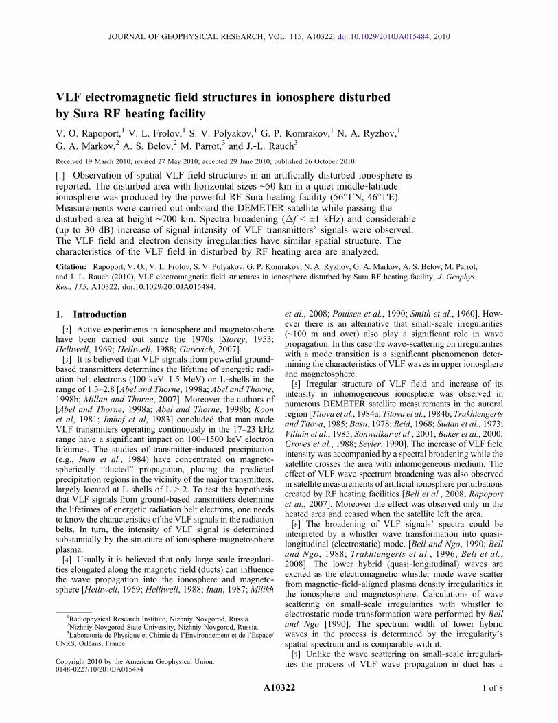
Figure 1. Electron density (Ne), VLF electric field (EVLF,frequency range of 17.6–19.1 kHz), and quasi‐static electricfield (EELF, frequency range of 0–1 kHz) as a function ofthe distance (in brackets) up to the center of the disturbedregion of field tube (the heated area). Figure 1a is relatedto the 1 May 2006 session whereas Figure 1b correspondsto the 17 May 2006 session.

RAPOPORT ET AL.: VLF STRUCTURES DISTURBED BY SURA FACILITY A10322A10322

2 of 8

the temperatures of the plasma component were registeredwith a time resolution of about 1 s. The sampling frequencyof electric and magnetic field detectors was 40,000 samplesper second. Ionosphere cutoff frequency f0(F2) and the mainparameters of the Sura facility during the experiment’ssessions are given in Table 1.[15] Figure 1a shows an electron density (Ne), intensity of

the VLF electric field in a frequency range of 17.6–19.1 kHz(EVLF), and the intensity of the quasi‐static electric field in arange of 0–1 kHz (EELF) over a 40 s time period for the 1May 2006 session. These data were acquired near themagnetic field line intersecting the heating area of the Surafacility. Figure 1b is the same for the 17 May 2006 session.In both sessions, the beginning of measurements in Burstmode was at 18:28:32 UT (22:28:32 LT).[16] From Figures 1a and 1b one can see that at the closest

approach to the center of the heated area both electrondensity of plasma and electric field intensity increase. Thesize of the perturbed electron density area is estimated as LN’ 45 km since time of satellite flight in the disturbed regionin about 6–7 s. The size of the increased electric field area isabout LE ’ 90–100 km and outside this area the intensity ofthe VLF field decreases abruptly by ∼30 dB.[17] The frequency‐time spectrogram of VLF electric field

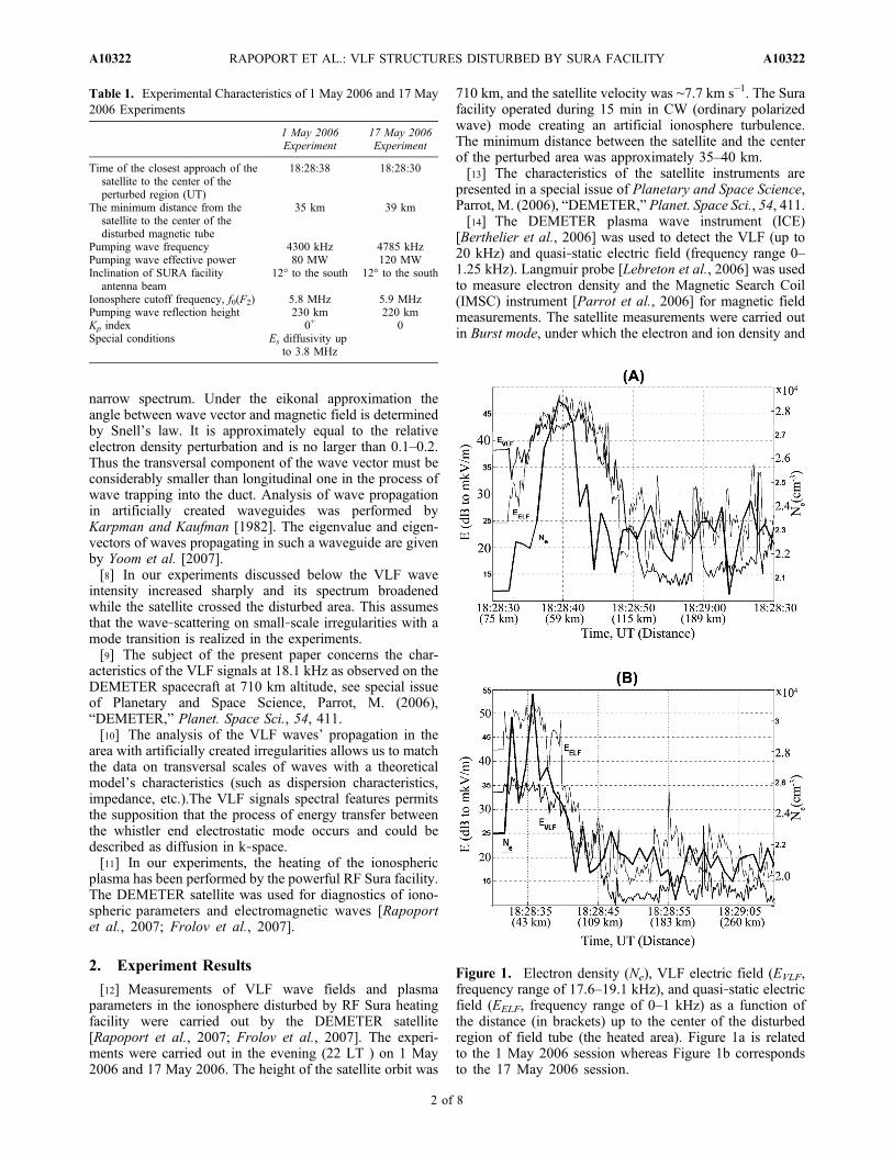
in a frequency range of 0–19.5 kHz is shown on Figure 2.This spectrogram is given for the 1 May 2006 experimentsession between 18:28:32 and 18:29:28 UT (distances to thecenter of the heated area are in brackets). Several VLFtransmitter signals were detected—a continuous wave (CW)signal at a frequency close to 18 kHz and a pulsing signal atfrequencies close to 12, 13, and 15 kHz. Ovals mark thefrequency broadening of CW VLF signal and quasi‐staticnoise caused by artificial ionosphere irregularities in theheated area.

[18] In the heated area of the ionosphere which DEMETERflew through at 18:28:33–18:28:45 UT (marked with verticallines) the intensity of CW VLF signal at 18 kHz significantlyincreases together with its spectrum width. Signal bandwidthfor this transmitter is as large as 1 kHz during this period.Spectra of pulsing VLF signals also broadened in the areaswith artificial ionosphere irregularities.[19] Figure 3 shows the sequence of electric and magnetic

fields’ power spectra measured in the disturbed area in afrequency range of 17.5–18.7 kHz. On each spectrum, theelectric field is shown by a thin line (the left scale of inten-sity, dB to 1 mV/m Hz1/2), and magnetic field is representedby a bold line (the right scale of intensity, dB to 1nT/Hz1/2).To compute spectra we used series of 10 data arrays of 0.2 sduration (spectral resolution ∼5 Hz) and then averaged thesepower spectra.[20] As one can see from Figure 3, the spectrum of the

VLF electric field consists of two components: a quasi‐monochromatic line at the VLF transmitter’s pumping wavefrequency (18.1 kHz) and a noise continuum with a maxi-mum at the same frequency and a bandwidth of about 0.4–0.5 kHz (at a 3 dB level). The noise continuum level increasesup to 30 dB in a bandwidth of ±0.3 kHz. At distances up to60 km from the center of disturbed area the carrier frequencyis masked by the noise level. At distances of 60–100 km theintensity of pumping frequency signal did not change, whilethe intensity of the noise continuummonotonously decreases.At distances of 100–130 km the signal decreases abruptly(by 30 dB).[21] Figure 4 shows the power spectra for the electrostatic

field (a continuous line for a frequency range of 0–1 kHz)and for the noise VLF continuum (2, 3). Here the VLFfrequency is counted both up and down from the pumpingfrequency (18.1 kHz). The dashed curve corresponds to the

Figure 2. The electric field frequency‐time spectrogram for 1 May 2006 session. Vertical lines mark thetime of DEMETER flight through the heated area. Signals of VLF stations (continuous wave and pulsing)are marked with arrows. The boundary at 8–11 kHz corresponds to LHR frequency.

RAPOPORT ET AL.: VLF STRUCTURES DISTURBED BY SURA FACILITY A10322A10322

3 of 8

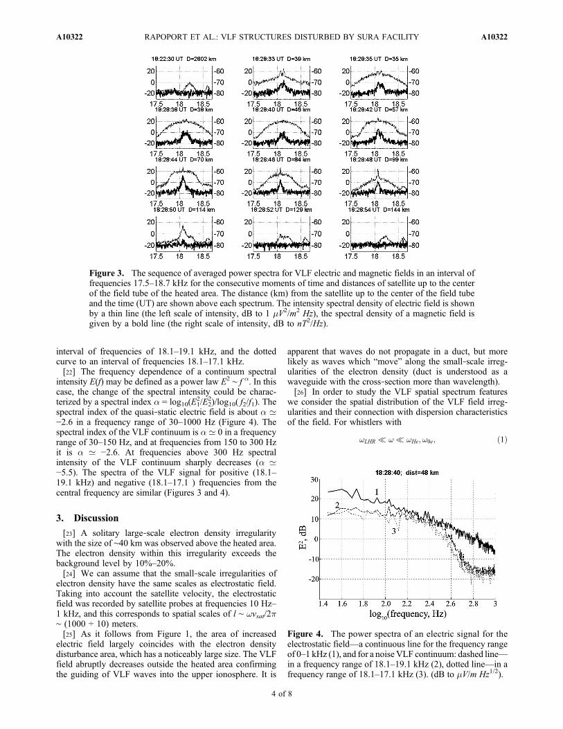
interval of frequencies of 18.1–19.1 kHz, and the dottedcurve to an interval of frequencies 18.1–17.1 kHz.[22] The frequency dependence of a continuum spectral

intensity E(f) may be defined as a power law E2 ∼ f a. In thiscase, the change of the spectral intensity could be charac-terized by a spectral index a = log10(E1

2/E22)/log10( f2/f1). The

spectral index of the quasi‐static electric field is about a ’−2.6 in a frequency range of 30–1000 Hz (Figure 4). Thespectral index of the VLF continuum is a ’ 0 in a frequencyrange of 30–150 Hz, and at frequencies from 150 to 300 Hzit is a ’ −2.6. At frequencies above 300 Hz spectralintensity of the VLF continuum sharply decreases (a ’−5.5). The spectra of the VLF signal for positive (18.1–19.1 kHz) and negative (18.1–17.1 ) frequencies from thecentral frequency are similar (Figures 3 and 4).

3. Discussion

[23] A solitary large‐scale electron density irregularitywith the size of ∼40 km was observed above the heated area.The electron density within this irregularity exceeds thebackground level by 10%–20%.[24] We can assume that the small‐scale irregularities of

electron density have the same scales as electrostatic field.Taking into account the satellite velocity, the electrostaticfield was recorded by satellite probes at frequencies 10 Hz–1 kHz, and this corresponds to spatial scales of l ∼ wvsat/2p∼ (1000 ÷ 10) meters.[25] As it follows from Figure 1, the area of increased

electric field largely coincides with the electron densitydisturbance area, which has a noticeably large size. The VLFfield abruptly decreases outside the heated area confirmingthe guiding of VLF waves into the upper ionosphere. It is

apparent that waves do not propagate in a duct, but morelikely as waves which “move” along the small‐scale irreg-ularities of the electron density (duct is understood as awaveguide with the cross‐section more than wavelength).[26] In order to study the VLF spatial spectrum features

we consider the spatial distribution of the VLF field irreg-ularities and their connection with dispersion characteristicsof the field. For whistlers with

!LHR � ! � !He; !0e; ð1Þ

Figure 3. The sequence of averaged power spectra for VLF electric and magnetic fields in an interval offrequencies 17.5–18.7 kHz for the consecutive moments of time and distances of satellite up to the centerof the field tube of the heated area. The distance (km) from the satellite up to the center of the field tubeand the time (UT) are shown above each spectrum. The intensity spectral density of electric field is shownby a thin line (the left scale of intensity, dB to 1 mV2/m2 Hz), the spectral density of a magnetic field isgiven by a bold line (the right scale of intensity, dB to nT2/Hz).

Figure 4. The power spectra of an electric signal for theelectrostatic field—a continuous line for the frequency rangeof 0–1 kHz (1), and for a noise VLF continuum: dashed line—in a frequency range of 18.1–19.1 kHz (2), dotted line—in afrequency range of 18.1–17.1 kHz (3). (dB to mV/m Hz1/2).

RAPOPORT ET AL.: VLF STRUCTURES DISTURBED BY SURA FACILITY A10322A10322

4 of 8

(where w is frequency of the VLF waves, wHe and w0e areelectron gyrofrequency and plasma frequency, respectively,and wLHR the lower hybrid resonance frequency), all com-ponents of dielectric permeability tensor are proportional tothe electron density [Karpman and Kaufman, 1982]. Thedispersion equation for the VLF waves with the condition(1) is as follows Karpman and Kaufman [1983a and 1983b]and:

n2? ¼ 2u2� ��1

1� 2u2� �

n2k � 2a�ffiffiffiffiffiffiffiffiffiffiffiffiffiffiffiffiffiffiffiffin4k � 4an2k

qh i; ð2Þ

(where k0 = w/c is the wave number in vacuum, a = w0e2 /wHe

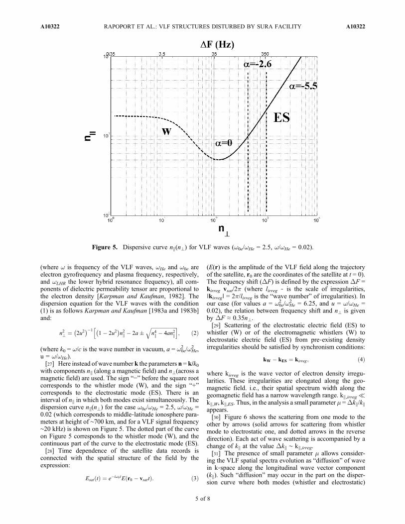
2 ,u = w/wHe).[27] Here instead of wave number k the parameters n = k/k0

with components nk (along a magnetic field) and n?(across amagnetic field) are used. The sign “−” before the square rootcorresponds to the whistler mode (W), and the sign “+”corresponds to the electrostatic mode (ES). There is aninterval of nk in which both modes exist simultaneously. Thedispersion curve nk(n?) for the case w0e/wHe = 2.5, w/wHe =0.02 (which corresponds to middle‐latitude ionosphere para-meters at height of ∼700 km, and for a VLF signal frequency∼20 kHz) is shown on Figure 5. The dotted part of the curveon Figure 5 corresponds to the whistler mode (W), and thecontinuous part of the curve to the electrostatic mode (ES).[28] Time dependence of the satellite data records is

connected with the spatial structure of the field by theexpression:

Esat tð Þ ¼ e�i!0 tE r0 � vsattð Þ: ð3Þ

(E(r) is the amplitude of the VLF field along the trajectoryof the satellite, r0 are the coordinates of the satellite at t = 0).The frequency shift (DF) is defined by the expression DF =kirreg vsat/2p (where lirreg ‐ is the scale of irregularities,∣kirreg∣ = 2p/lirreg is the “wave number” of irregularities). Inour case (for values a = w0e

2 /wHe2 = 6.25, and u = w/wHe =

0.02), the relation between frequency shift and n? is givenby DF ≈ 0.35n?.[29] Scattering of the electrostatic electric field (ES) to

whistler (W) or of the electromagnetic whistlers (W) toelectrostatic electric field (ES) from pre‐existing densityirregularities should be satisfied by synchronism conditions:

kW � kES ¼ kirreg; ð4Þ

where kirreg is the wave vector of electron density irregu-larities. These irregularities are elongated along the geo-magnetic field. i.e., their spatial spectrum width along thegeomagnetic field has a narrow wavelength range. kk,irreg �kk,W, kk,ES. Thus, in the analysis a small parameter m =Dkk/kkappears.[30] Figure 6 shows the scattering from one mode to the

other by arrows (solid arrows for scattering from whistlermode to electrostatic one, and dotted arrows in the reversedirection). Each act of wave scattering is accompanied by achange of kk at the value Dkk ∼ kk,irreg.[31] The presence of small parameter m allows consider-

ing the VLF spatial spectra evolution as “diffusion” of wavein k‐space along the longitudinal wave vector component(kk). Such “diffusion” may occur in the part on the disper-sion curve where both modes (whistler and electrostatic)

Figure 5. Dispersive curve nk(n?) for VLF waves (w0e/wHe = 2.5, w/wHe = 0.02).

RAPOPORT ET AL.: VLF STRUCTURES DISTURBED BY SURA FACILITY A10322A10322

5 of 8

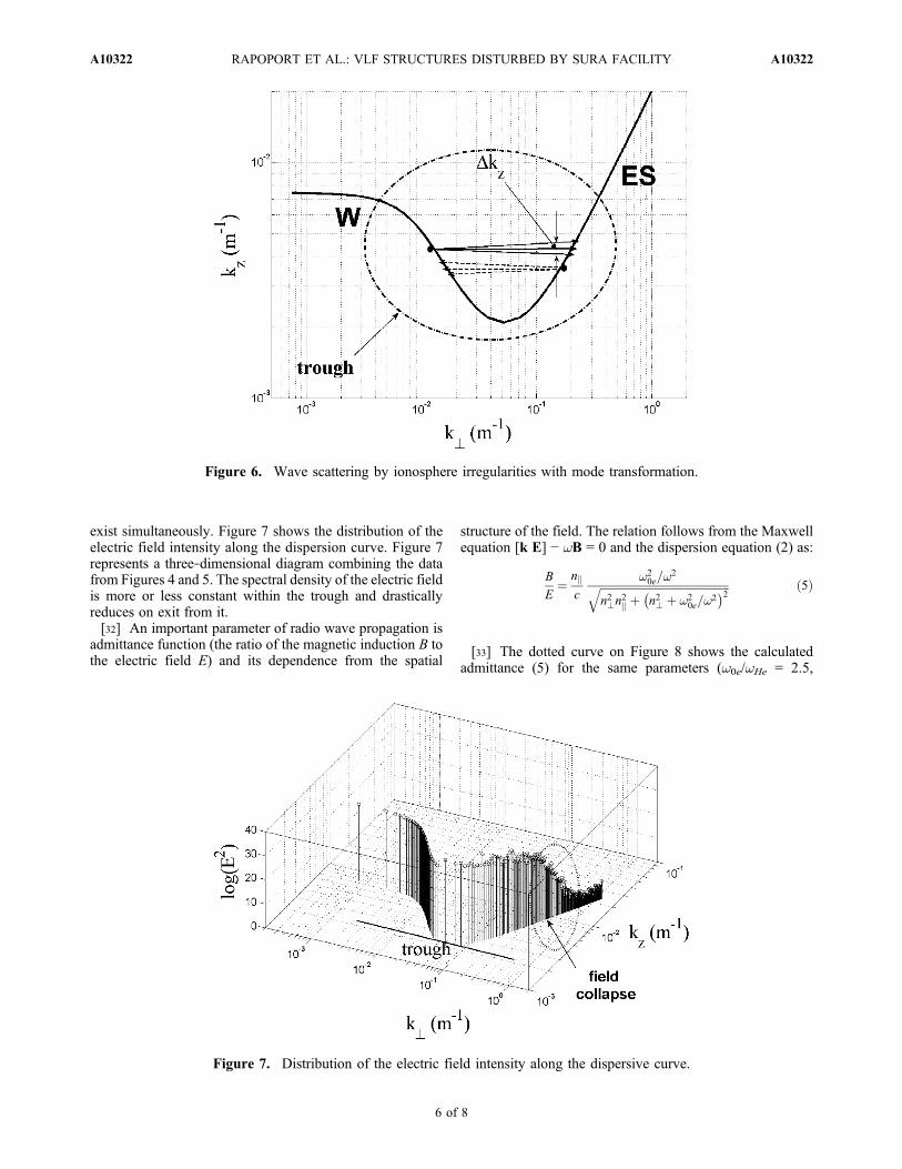
exist simultaneously. Figure 7 shows the distribution of theelectric field intensity along the dispersion curve. Figure 7represents a three‐dimensional diagram combining the datafrom Figures 4 and 5. The spectral density of the electric fieldis more or less constant within the trough and drasticallyreduces on exit from it.[32] An important parameter of radio wave propagation is

admittance function (the ratio of the magnetic induction B tothe electric field E) and its dependence from the spatial

structure of the field. The relation follows from the Maxwellequation [k E] − wB = 0 and the dispersion equation (2) as:

B

E¼ nk

c

!20e=!

2

ffiffiffiffiffiffiffiffiffiffiffiffiffiffiffiffiffiffiffiffiffiffiffiffiffiffiffiffiffiffiffiffiffiffiffiffiffiffiffiffiffiffiffiffiffiffiffin2?n

2k þ n2? þ !2

0e=!2

� �2q ð5Þ

[33] The dotted curve on Figure 8 shows the calculatedadmittance (5) for the same parameters (w0e/wHe = 2.5,

Figure 6. Wave scattering by ionosphere irregularities with mode transformation.

Figure 7. Distribution of the electric field intensity along the dispersive curve.

RAPOPORT ET AL.: VLF STRUCTURES DISTURBED BY SURA FACILITY A10322A10322

6 of 8

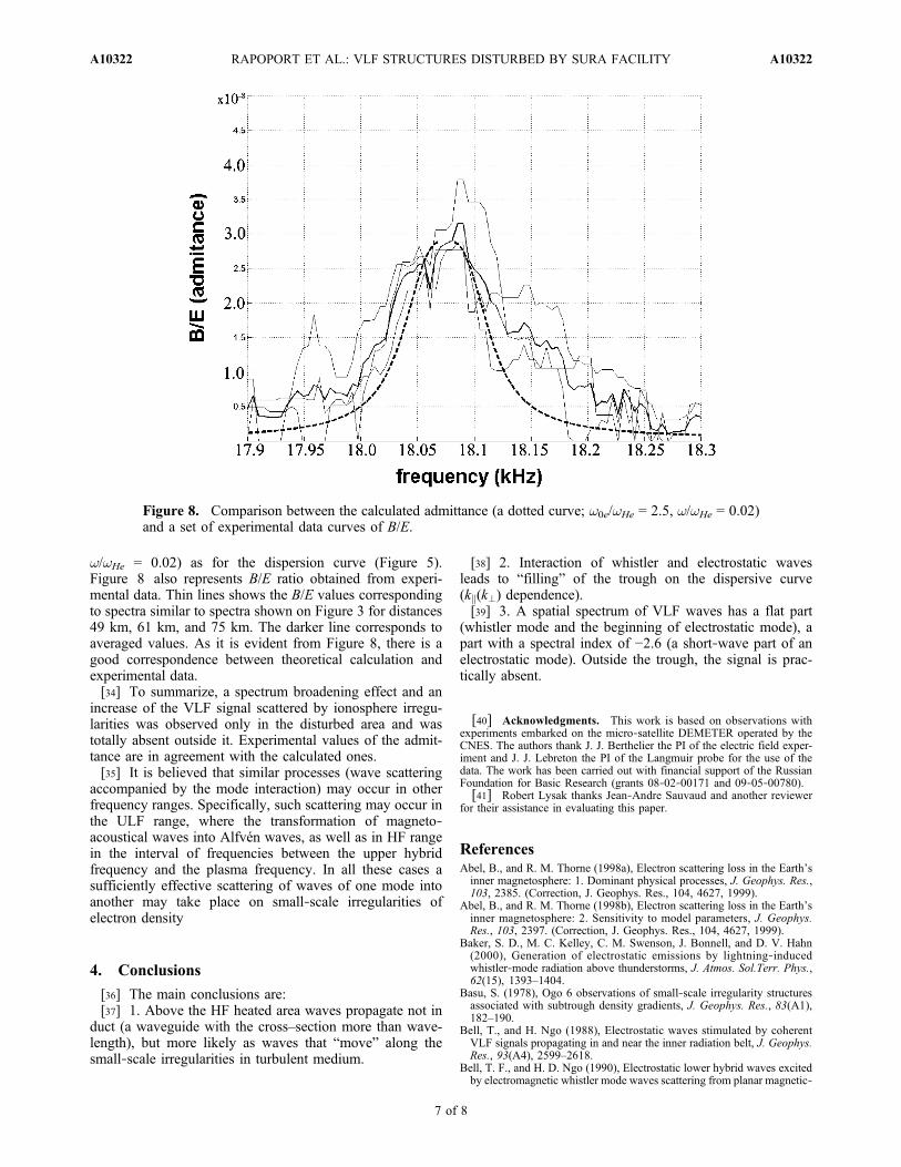
w/wHe = 0.02) as for the dispersion curve (Figure 5).Figure 8 also represents B/E ratio obtained from experi-mental data. Thin lines shows the B/E values correspondingto spectra similar to spectra shown on Figure 3 for distances49 km, 61 km, and 75 km. The darker line corresponds toaveraged values. As it is evident from Figure 8, there is agood correspondence between theoretical calculation andexperimental data.[34] To summarize, a spectrum broadening effect and an

increase of the VLF signal scattered by ionosphere irregu-larities was observed only in the disturbed area and wastotally absent outside it. Experimental values of the admit-tance are in agreement with the calculated ones.[35] It is believed that similar processes (wave scattering

accompanied by the mode interaction) may occur in otherfrequency ranges. Specifically, such scattering may occur inthe ULF range, where the transformation of magneto‐acoustical waves into Alfvén waves, as well as in HF rangein the interval of frequencies between the upper hybridfrequency and the plasma frequency. In all these cases asufficiently effective scattering of waves of one mode intoanother may take place on small‐scale irregularities ofelectron density

4. Conclusions

[36] The main conclusions are:[37] 1. Above the HF heated area waves propagate not in

duct (a waveguide with the cross–section more than wave-length), but more likely as waves that “move” along thesmall‐scale irregularities in turbulent medium.

[38] 2. Interaction of whistler and electrostatic wavesleads to “filling” of the trough on the dispersive curve(kk(k?) dependence).[39] 3. A spatial spectrum of VLF waves has a flat part

(whistler mode and the beginning of electrostatic mode), apart with a spectral index of −2.6 (a short‐wave part of anelectrostatic mode). Outside the trough, the signal is prac-tically absent.

[40] Acknowledgments. This work is based on observations withexperiments embarked on the micro‐satellite DEMETER operated by theCNES. The authors thank J. J. Berthelier the PI of the electric field exper-iment and J. J. Lebreton the PI of the Langmuir probe for the use of thedata. The work has been carried out with financial support of the RussianFoundation for Basic Research (grants 08‐02‐00171 and 09‐05‐00780).[41] Robert Lysak thanks Jean‐Andre Sauvaud and another reviewer

for their assistance in evaluating this paper.

ReferencesAbel, B., and R. M. Thorne (1998a), Electron scattering loss in the Earth’sinner magnetosphere: 1. Dominant physical processes, J. Geophys. Res.,103, 2385. (Correction, J. Geophys. Res., 104, 4627, 1999).

Abel, B., and R. M. Thorne (1998b), Electron scattering loss in the Earth’sinner magnetosphere: 2. Sensitivity to model parameters, J. Geophys.Res., 103, 2397. (Correction, J. Geophys. Res., 104, 4627, 1999).

Baker, S. D., M. C. Kelley, C. M. Swenson, J. Bonnell, and D. V. Hahn(2000), Generation of electrostatic emissions by lightning‐inducedwhistler‐mode radiation above thunderstorms, J. Atmos. Sol.Terr. Phys.,62(15), 1393–1404.

Basu, S. (1978), Ogo 6 observations of small‐scale irregularity structuresassociated with subtrough density gradients, J. Geophys. Res., 83(A1),182–190.

Bell, T., and H. Ngo (1988), Electrostatic waves stimulated by coherentVLF signals propagating in and near the inner radiation belt, J. Geophys.Res., 93(A4), 2599–2618.

Bell, T. F., and H. D. Ngo (1990), Electrostatic lower hybrid waves excitedby electromagnetic whistler mode waves scattering from planar magnetic‐

Figure 8. Comparison between the calculated admittance (a dotted curve; w0e/wHe = 2.5, w/wHe = 0.02)and a set of experimental data curves of B/E.

RAPOPORT ET AL.: VLF STRUCTURES DISTURBED BY SURA FACILITY A10322A10322

7 of 8

field‐aligned plasma density irregularities, J. Geophys. Res., 95(A1),149–172.

Bell, T. F., U. S. Inan, D. Piddyachiy, P. Kulkarni, and M. Parrot (2008),Effects of plasma density irregularities on the pitch angle scattering ofradiation belt electrons by signals from ground based VLF transmitters,Geophys. Res. Lett., 35, L19103, doi:10.1029/2008GL034834.

Berthelier, J. J., et al. (2006), ICE, The electric field experiment onDEMETER, Planet. Space Sci., 54, 456–471.

Frolov, V. L., et al. (2007), Modification of the earth’s ionosphere by high‐power high‐frequency radio waves, Phys. Usp., 50(3), 315–324.

Groves, K., M. Lee, and S. Kuo (1988), Spectral broadening of VLFradio signals traversing the ionosphere, J. Geophys. Res., 93(A12),14,683–14,687.

Gurevich, A. V. (2007), Nonlinear effects in the ionosphere, Phys. Usp.,50(11), 1091–1121.

Helliwell, R. A. (1969), Low‐frequency waves in the magnetosphere,Rev. Geophys., 7(1,2), 281–303.

Helliwell, R. A. (1988), VLF wave stimulation experiments in the magne-tosphere from Siple Station, Antarctica, Rev. Geophys., 26(3), 551–578.

Inan, U. S. (1987), Waves and instabilities, Rev. Geophys., 25(3), 588–598.Inan, U., H. Chang, and R. Helliwell (1984), Electron precipitation zonesaround major ground‐based VLF signal sources, J. Geophys. Res.,89(A5), 2891–2906.

Imhof, W. L., J. B. Reagan, H. D. Voss, E. E. Gaines, D. W. Datlowe,J. Mobilia, R. A. Helliwell, U.S. Inan, J. Katsufrakis, and R. G. Joiner(1983), The modulated precipitation of radiation belt electrons by con-trolled signals from ground‐based transmitters, Geophys. Res. Lett.,10, 615.

Karpman, V. I., and R. N. Kaufman (1982), Whistler wave propagation indensity ducts, J. Plasma Phys., 27(02), 225–238.

Karpman, V. I., and R. N. Kaufman (1983a), Peculiarities of whistlerwave’s propagation in magnetosphere ducts in subequatorial area. I.Ducts with increased density, Geomagn. Aeron., 23, 451–457.

Karpman, V. I., and R. N. Kaufman (1983b), Peculiarities of whistlerwave’s propagation in magnetosphere ducts in subequatorial area. II.Ducts with decreased density, Geomagn. Aeron., 23, 791–796.

Koon, H. C., B. C. Edgar, and A. L. Vampola (1981), Precipitation of innerzona electrons by whistler mode waves from the VLF transmitters UMSand NWC, J. Geophys. Res., 86(A2), 640–648.

Lebreton, J.‐P., et al. (2006), The ISL Langmuir probe experiment pro-cessing onboard DEMETER: Scientific objectives, description and firstresults, Planet. Space Sci., 54, 472–486.

Milikh, G. M., K. Papadopoulos, H. Shroff, C. L. Chang, T. Wallace,E. V. Mishin, M. Parrot, and J. J. Berthelier (2008), Formation of artificialionospheric ducts, Geophys. Res. Lett., 35, L17104, doi:10.1029/2008GL034630.

Millan, R. M., and R. M. Thorne (2007), Review of radiation belt rela-tivistic electron losses, J. Atmos. Sol.Terr. Phys., 69, 362.

Parrot, M., et al. (2006), The magnetic field experiment IMSC and its dataprocessing onboard DEMETER: Scientific objectives, description andfirst results, Planet. Space Sci., 54, 441–455, doi:10.1016/j.pss.2005.10.015.

Poulsen, W., T. Bell, and U. Inan (1990), Three‐Dimensional modeling ofsubionospheric VLF propagation in the presence of localized D region

perturbations associated with lightning, J. Geophys. Res., 95(A3),2355–2366.

Rapoport, V. O., V. L. Frolov, G. P. Komrakov, G. A. Markov, A. S. Belov,M. Parrot, and J. L. Rauch (2007), Some results of measuring the charac-teristics of electromagnetic and plasma disturbances stimulated in theouter ionosphere by high‐power high‐frequency radio emission fromthe “Sura” facility, Radiophysics Quantum Electri., 50(8), 645–656.

Reid, G. (1968), The formation of small‐scale irregularities in the iono-sphere, J. Geophys. Res., 73(5), 1627–1640.

Seyler, C. (1990), A mathematical model of the structure and evolutionof small‐scale discrete auroral arcs, J. Geophys. Res., 95(A10),17,199–17,215.

Smith, R. L., R. A. Helliwell, and I. W. Yabroff (1960), A theory of trap-ping of whistlers in field‐aligned columns of enchanced ionization,J. Geophys. Res., 65(3), 815.

Sonwalkar, V. S., X. Chen, J. Harikumar, D. L. Carpenter, and T. F Bell.(2001), Whistler‐mode wave‐injection experiments in the plasmaspherewith a radio sounder, J. Atmos. Sol.Terr. Phys., 63(11), 1199–1216.

Storey, L. R. O. (1953), An investigation of whistling atmospherics. Phil.Trans. R. Soc. London, Ser. A, 246, 113–141.

Sudan, R., J. Akinrimisi, and D. Farley (1973), Generation of small‐scale irregularities in the equatorial electrojet, J. Geophys. Res., 78(1),240–248.

Titova, E. E., V. I. Di, V. E. Yurov, O. M. Raspopov, V. Yu. Trakhtengertz,F. Jiricek, and P. Triska (1984a), Interaction between VLF waves and theturbulent ionosphere, Geophys. Res. Lett., 11(4), 323–326.

Titova, E. E., V. I. Di, F. Jiricek, I. V. Lychkina, O. M. Raspopov, V. Yu.Trakhtengertz, P. Triska, and V. E. Yurov (1984b), VLF transmitters’spectra broadening in upper ionosphere, Geomagn. Aeron., 24(6),935–943.

Trakhtengerts, V. Yu., and E. E. Titova (1985), Interaction of monochro-matic VLF waves with the turbulent ionosphere, Geomagn. Aeron.,25(1), 89–96.

Trakhtengerts, V., M. Rycroft, and A. Demekhov (1996), Interrelation ofnoise‐like and discrete ELF/VLF emissions generated by cyclotron inter-actions, J. Geophys. Res., 101(A6), 13,293–13,301.

Villain, J., G. Caudal, and C. Hanuise (1985), A Safari‐Eiscat comparisonbetween the velocity of F region small‐scale irregularities and the iondrift, J. Geophys. Res., 90(A9), 8433–8443.

Yoom, P. H., S. Ye. LaBelle, A. T. Weatherwax, and J. D. Menietti (2007),Methods in the study of discrete upper hybrid waves, J. Geophys. Res.,112, A11305, doi:10.1029/2007JA012683.

Yurov, V. E. (1984), VLF transmitters’ spectra broadening in upper iono-sphere, Geomagn. Aeron., 24(6), 935–943.

A. S. Belov and G. A. Markov, Nizhniy Novgorod State University,Nizhniy Novgorod, Russia.V. L. Frolov, G. P. Komrakov, S. V. Polyakov, V. O. Rapoport, and

N. A. Ryzhov, Radiophysical Research Institute, Nizhniy Novgorod,Russia. (wrapoport@nirfi.sci‐nnov.ru)M. Parrot and J.‐L. Rauch, Laboratorie de Physique et Chimie de

l’Environnement et de l’Espace/CNRS, Orléans, France.

RAPOPORT ET AL.: VLF STRUCTURES DISTURBED BY SURA FACILITY A10322A10322

8 of 8