Astronomy & Astrophysics manuscript no. Antares˙PIONIER˙v5r0˙prod c© ESO 2018March 14, 2018

The convective surface of the red supergiant Antares?

VLTI/PIONIER interferometry in the near infraredM. Montarges1, A. Chiavassa2, P. Kervella3,4, S. T. Ridgway5, G. Perrin4, J.-B. Le Bouquin6, and S. Lacour4

1 Institut de Radioastronomie Millimetrique, 300 rue de la Piscine, 38406, Saint Martin d’Heres, France2 Universite Cote dâĂŹAzur, Observatoire de la Cote dâĂŹAzur, CNRS, Lagrange, CS 34229, Nice, France3 Unidad Mixta Internacional Franco-Chilena de Astronomıa (UMI 3386), CNRS/INSU, France & Departamento de

Astronomıa, Universidad de Chile, Camino El Observatorio 1515, Las Condes, Santiago, Chile.4 LESIA, Observatoire de Paris, PSL Research University, CNRS UMR 8109, Sorbonne Universites, UPMC, Universite

Paris Diderot, Sorbonne Paris Cite, 5 place Jules Janssen, F-92195 Meudon, France5 National Optical Astronomy Observatories, 950 North Cherry Avenue, Tucson, AZ 85719, USA6 UJF-Grenoble 1/CNRS-INSU, Institut de Planetologie et d’Astrophysique de Grenoble (IPAG), UMR 5274, Grenoble,

France

Received 31 Oct. 2016; Accepted 15 May 2017

ABSTRACT

Context. Convection is a candidate to explain the trigger of red supergiant star (RSG) mass loss. Owing to the smallsize of the convective cells on the photosphere, few of the characteristics of RSGs are known.Aims. Using near infrared interferometry, we intend to resolve the photosphere of RSGs and to bring new constraintson their modeling.Methods. We observed the nearby red supergiant Antares using the four-telescope instrument VLTI/PIONIER. Wecollected data on the three available configurations of the 1.8m telescopes in the H band.Results. We obtained unprecedented angular resolution on the disk of a star (6% of the star angular diameter) thatlimits the mean size of convective cells and offers new constraints on numerical simulations. Using an analytical modelwith a distribution of bright spots we determine their effect on the visibility signal.Conclusions. We determine that the interferometric signal on Antares is compatible with convective cells of various sizesfrom 45% to 5% of the angular diameter. We also conclude that convective cells can strongly affect the angular diameterand limb-darkening measurements. In particular, the apparent angular diameter becomes dependent on the sampledposition angles.

Key words. Stars: individual: Antares; Stars: imaging; Stars: supergiants; Stars: mass-loss; Infrared: Stars; Techniques:interferometric

1. IntroductionChemical enrichment of the Universe is driven by evolvedstars. Although currently rare, massive stars were muchmore numerous during the early times of the Universe.When entering the red supergiant (RSG) phase in theirlater evolution, these stars experience intense mass loss.The material expelled from the star cools, allowing the for-mation of molecules and dust that will be essential con-tributions to new stellar systems. However, the processesdriving this outflow of material remain only partly under-stood.

RSG stars do not experience flares or large-scale pulsa-tions that could inject enough momentum for the materialto be launched away from the star. Arroyo-Torres et al.(2015) demonstrated that pulsation models do not repro-duce the molecular extension of the atmosphere of RSGthat would be consistent with their mass loss. Harper (2010)stated that there is no available physical scenario that canbe shown to initiate the outflow of massive evolved stars.

? Based on observations made with ESO telescopes at ParanalObservatory, under ESO programs 093.D-0378(A), 093.D-0378(B), 093.D-0378(C) and 093.D-0673(C).

Schwarzschild (1975) predicted that, compared to thesun, the photosphere of RSG could be host to a smallernumber of much larger convective cells. From spectroscopicobservations of a sample of RSGs, Josselin & Plez (2007)proposed that large convective cells could trigger mass lossby locally lowering the effective gravity and allowing radia-tive pressure on molecular lines to initiate the outflow.

Early imaging observations offered further evidence forconvective activity. Only two large hot spots were detectedover the visible hemisphere of Betelgeuse by Haubois et al.(2009) in a high-dynamic-range reconstructed image fromIOTA H band interferometric observations. Chiavassaet al. (2010b, hereafter C10b) identified a possible con-vective pattern in the same dataset using 3D radiativehydrodynamics simulations (RHD).

Antares (α Sco, HD 148478, HR 6134) is the closestRSG (π = 5.89±1.00 mas, van Leeuwen 2007). Its apparentdiameter of ∼ 37 mas, measured from VLTI/AMBER databy Ohnaka et al. (2013, hereafter O13), makes it one ofthe largest stars in our sky. The same authors derived amass of 15±5 M� and an age of 11-15 Myr. It is a classicalRSG with a spectral type M0.5Iab. It has a B3V companion

1

arX

iv:1

705.

0782

9v2

[as

tro-

ph.S

R]

14

Sep

2017

M. Montarges et al.: The convective surface of Antares

(Antares B) located far enough away (2.7”, Ohnaka 2014)that we can consider the primary alone in the present study.

Around this RSG, O13 observed upward and down-ward motions of CO in the upper atmosphere or near cir-cumstellar region (1.3 R?), strongly pointing towards aconvection-based mechanism. Observations of the circum-stellar environment of Antares by Ohnaka (2014) using theVLT/VISIR instrument revealed a clumpy and dusty en-velope. This is compatible with convection-triggered massloss.

Pugh & Gray (2013) studied the short timescale radialvelocity variations of the star. In addition to large hotspots, reported earlier on RSG, they suggested that thisobservation could be associated to smaller-scale convectiveactivity. Stothers (2010) showed that the long secondaryphotometric period of RSGs, and in particular of Antares,could be related to convection. Therefore we see that thereare several reasons for suspecting the importance of con-vection in RSG atmospheres, and for hypothesizing that itis triggering the mass loss. However, an observational basisfor constraining the spatial scale of convection is neededfor empirical and theoretical modeling of the mass loss.

Until now, near-infrared interferometric observationsof RSGs have only probed the spatial frequencies up tothe fifth or sixth lobe of the visibility function at most.Convective simulations from Chiavassa et al. (2011, here-after C11a) predicted that the convective cell structurescould enhance the visibility signal up to the tenth lobe atleast. The smaller granules detected at those high spatialfrequencies are expected to be more numerous. They haveyet to be detected with optical interferometry. This isessential to minimally constrain the surface convectionpattern on RSGs.

Interferometry is the only way to obtain detailed ob-servations of the photospheric region of RSGs. We presentVLTI/PIONIER observations of Antares at a very high an-gular resolution (∼ 1/15th of the stellar radius). In Sect. 2we present our observations and the data reduction. We fitthe data with analytical models in Sect. 3, ranging fromclassical disks to a distribution of models that includesbright Gaussian spots. We continue the analysis with 3Dradiative hydrodynamics simulations in Sect. 4.

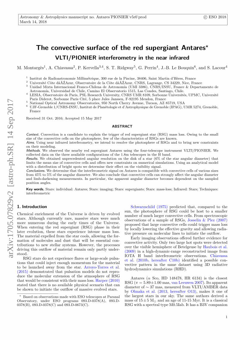
2. ObservationsTo observe Antares, we used the European SouthernObservatory’s Very Large Telescope Interferometer (VLTI,Haguenauer et al. 2010) located on top of Cerro Paranal inNorthern Chile with the PIONIER instrument (PrecisionIntegrated-Optics Near-infrared Imaging ExpeRiment, LeBouquin et al. 2011), which recombines the light of fourtelescopes simultaneously. We observed with the four 1.8 mdiameter Auxiliary Telescopes (AT) of the VLTI in threedifferent configurations that gave us access to baselinesfrom 11.3 m to 153.0 m on the ground. The resulting(u, v) coverage is represented in Fig. 1. The instrumentwas configured in the high spectral resolution mode (R∼ 40) that produces seven spectral channels over the Hband (1.54− 1.80 µm). To avoid saturation, without usinga neutral density, we read only the three central pixels ofthe detector (1.60 − 1.71 µm). Antares and its calibratorswere observed on 2014 April 24, 29 and May 4 and 7.

15010050050100150U (m)

150

100

50

0

50

100

150

V (

m)

0.0

0.1

0.2

0.3

0.4

0.5

0.6

0.7

0.8

0.9

1.0

Fig. 1. (u, v) coverage of our VLTI/PIONIER observationsof Antares. North is up and East is left. The compactAT configuration is represented with the green circles, themedium configuration with the blue triangles and the ex-tended configuration is represented with the red squares.Underneath, the visibility amplitude of a power-law limb-darkened disk matching the best fit parameters for Antaresat 1.61 µm is represented (see Sect 3).

Table 1. Adopted uniform disk diameters for the interfero-metric calibrators. (Bonneau et al. 2006, 2011 and Merandet al. 2005)

Name Diameter(mas)

HR 5969 1.79 ± 0.13HR 6145 0.84 ± 0.06HD 142407 1.27 ± 0.09HD 143900 1.28 ± 0.05HD 148643 1.47 ± 0.08ψ Oph 1.89 ± 0.13

The data were reduced using the publicly availablePIONIER pipeline (Le Bouquin et al. 2011). We adoptedthe angular diameters of Table 1 for the calibrators, ob-tained using the JMMC tool SearchCal1 (Bonneau et al.2006, 2011). The pipeline automatically computes the un-certainties: on the uncalibrated data it derives the statisti-cal dispersion over 100 scans each of ∼ 30 s exposure. Thenfor the calibrated product it quadratically adds the errorfrom the transfer function. As PIONIER is a four-telescopeinstrument, we finally got six squared visibility and four clo-sure phase measurements per observation and per spectralchannel. We had to ignore the data from baseline A1-K0because of their poor signal to noise ratio.

1 Available at http://www.jmmc.fr/searchcal

2

M. Montarges et al.: The convective surface of Antares

1.50 1.55 1.60 1.65 1.70 1.75Wavelength (µm)

2.4

2.6

2.8

3.0

3.2

3.4

3.6

3.8

Inte

nsi

ty (

x 1

0−

11 W

.m−

2.µ

m−

1)

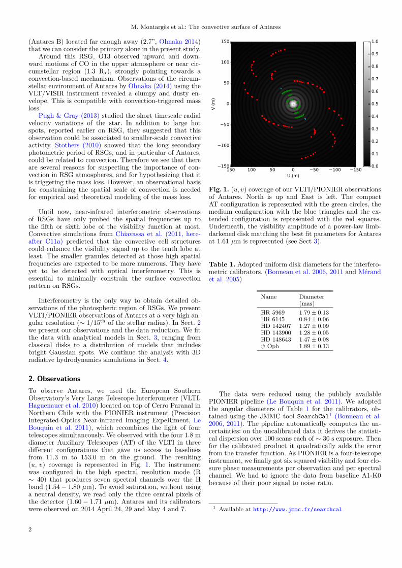
Fig. 2. Spectrum of the M0Ib-II star HD236697, in the Hband, from the Infrared Telescope Facility spectral library(Rayner et al. 2009). The PIONIER spectral channels areindicated with colored horizontal lines.

3. Analytical model analysis3.1. Classical disk models

To derive the angular diameter of the star, we use two dif-ferent models that are commonly employed in the litera-ture for RSGs: a uniform disk (UD) and a power law limb-darkened disk (LDD, with I(µ)/I0 = µδ). The squared vis-ibility of the later is given by Hestroffer (1997) :

VLDD(u, v) = Γ(ν + 1) Jν(x)(x/2)ν , (1)

where ν = δ/2 + 1 and Γ is the Euler function.No bandwidth smearing was used in any of the following

fits as tests showed that its effect kept the derived valueswithin their error bars.

We first fitted the entire squared visibility dataset (allbaseline lengths and spectral channels). However we noticedimportant positive deviations from the simple disk modelsindicating the presence of small additional features on thestellar surface. The reduced χ2 (χ2 hereafter) reaches ∼ 180for the UD model and ∼ 25 for the LDD.

To avoid the contamination of possible small scale fea-tures (also suggested by the closure phase deviations from0◦ or 180◦ on Fig. 5), we then only fitted the first lobe of thesquared visibility function (spatial frequencies lower than35 arcsec−1) for the UD model and the first two lobes for theLDD model (spatial frequencies lower than 50 arcsec−1).The χ2 is ∼ 20 and ∼ 16, respectively, meaning that im-portant deviations from the models are present.

Our VLTI/PIONIER observations consist of three dis-tinct spectral channels probing various molecular lines (Fig.2). Fitting those three channels separately in the first andfirst two lobes for the UD and LDD models, respectively,lowers the χ2 to 18-56 for the UD and 7-10 for the LDD.Therefore, we can conclude that the star does not look thesame in these three different wavelengths in the H band.Still, some deviations cannot be reproduced by the models.

In addition to the spectral channels, our observationscover several position angle (PA) directions in the first andsecond lobes. Figure 3 represents the PA dependency ofthe squared visibilities in the first two lobes. Three areas

27.5 30.0 32.5 35.0 37.5 40.0 42.5 45.0 47.5Spatial frequency (arcsec 1)

10 4

10 3

10 2

Squa

red

visib

ility

502502550

40

20

0

20

4060

70

80

90

100

110

10.0

12.5

15.0

17.5

20.0

22.5

25.0

27.5

Posit

ion

angl

e (

)

Fig. 3. VLTI/PIONIER squared visibilities measured onAntares as a function of spatial frequency for the first twolobes. In the inset, the (u, v) coverage is represented inarcsec−1. In both sub-figures, the PA is color-coded.

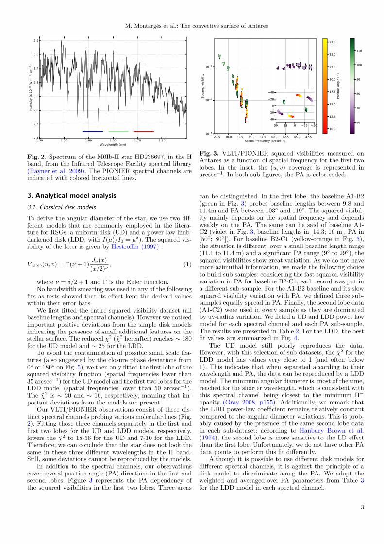
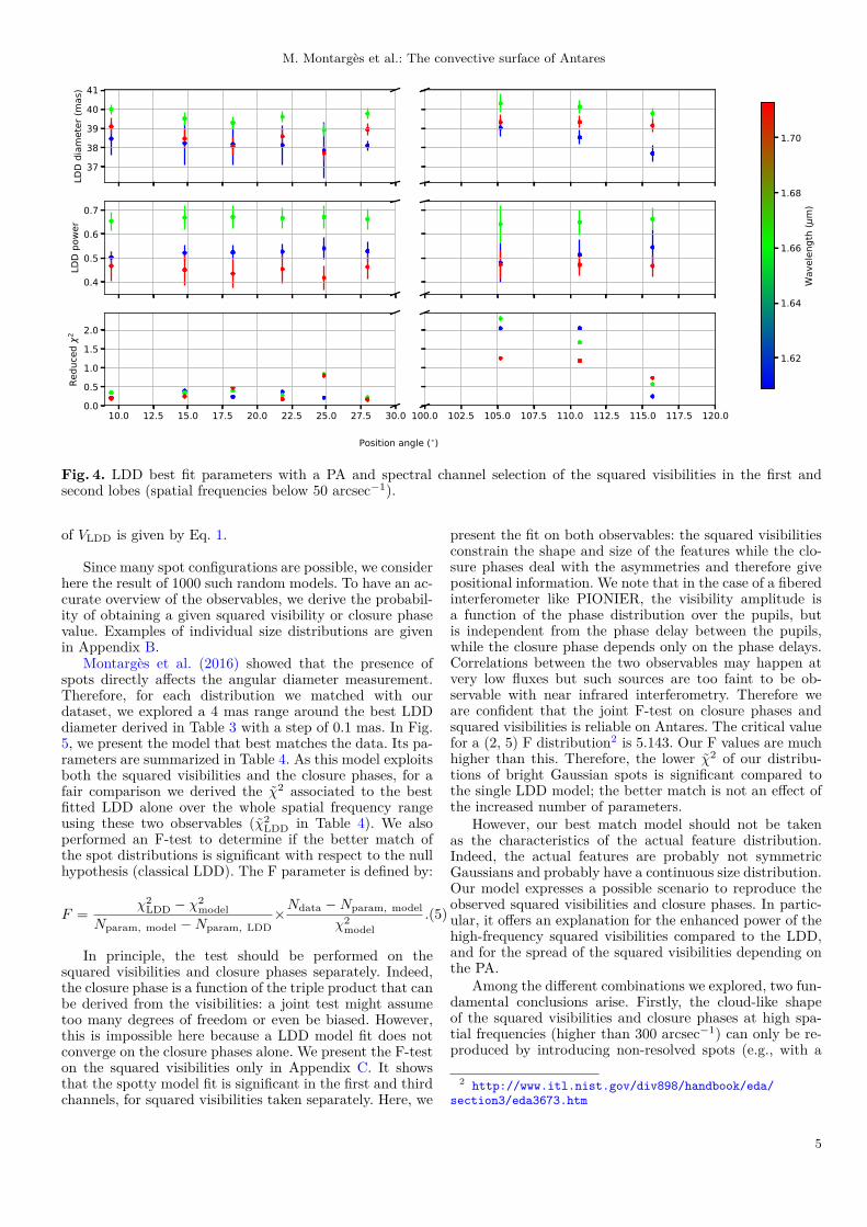
can be distinguished. In the first lobe, the baseline A1-B2(green in Fig. 3) probes baseline lengths between 9.8 and11.4m and PA between 103◦ and 119◦. The squared visibil-ity mainly depends on the spatial frequency and dependsweakly on the PA. The same can be said of baseline A1-C2 (violet in Fig. 3, baseline lengths in [14.3; 16 m], PA in[50◦; 80◦]). For baseline B2-C1 (yellow-orange in Fig. 3),the situation is different: over a small baseline length range(11.1 to 11.4 m) and a significant PA range (9◦ to 29◦), thesquared visibilities show great variation. As we do not havemore azimuthal information, we made the following choiceto build sub-samples: considering the fast squared visibilityvariation in PA for baseline B2-C1, each record was put ina different sub-sample. For the A1-B2 baseline and its slowsquared visibility variation with PA, we defined three sub-samples equally spread in PA. Finally, the second lobe data(A1-C2) were used in every sample as they are dominatedby uv-radius variation. We fitted a UD and LDD power lawmodel for each spectral channel and each PA sub-sample.The results are presented in Table 2. For the LDD, the bestfit values are summarized in Fig. 4.

The UD model still poorly reproduces the data.However, with this selection of sub-datasets, the χ2 for theLDD model has values very close to 1 (and often below1). This indicates that when separated according to theirwavelength and PA, the data can be reproduced by a LDDmodel. The minimum angular diameter is, most of the time,reached for the shorter wavelength, which is consistent withthis spectral channel being closest to the minimum H−

opacity (Gray 2008, p155). Additionally, we remark thatthe LDD power-law coefficient remains relatively constantcompared to the angular diameter variations. This is prob-ably caused by the presence of the same second lobe datain each sub-dataset: according to Hanbury Brown et al.(1974), the second lobe is more sensitive to the LD effectthan the first lobe. Unfortunately, we do not have other PAdata points to perform this fit differently.

Although it is possible to use different disk models fordifferent spectral channels, it is against the principle of adisk model to discriminate along the PA. We adopt theweighted and averaged-over-PA parameters from Table 3for the LDD model in each spectral channel.

3

M. Montarges et al.: The convective surface of Antares

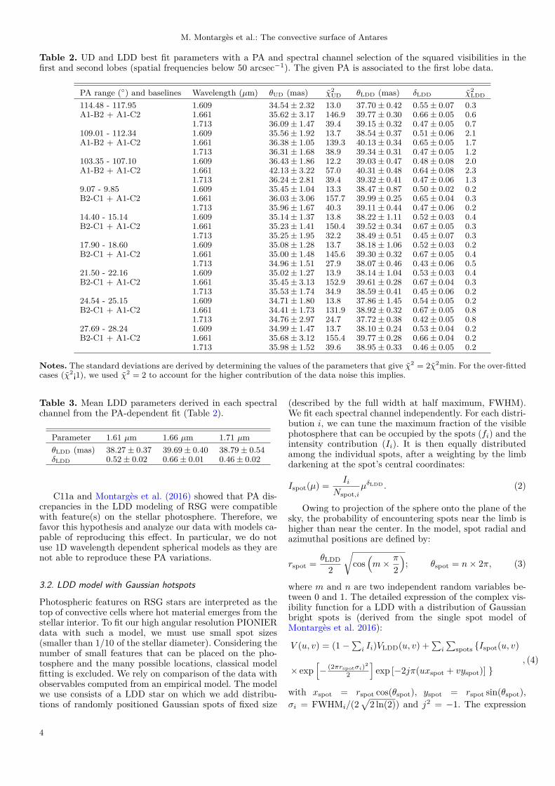
Table 2. UD and LDD best fit parameters with a PA and spectral channel selection of the squared visibilities in thefirst and second lobes (spatial frequencies below 50 arcsec−1). The given PA is associated to the first lobe data.

PA range (◦) and baselines Wavelength (µm) θUD (mas) χ2UD θLDD (mas) δLDD χ2

LDD

114.48 - 117.95 1.609 34.54 ± 2.32 13.0 37.70 ± 0.42 0.55 ± 0.07 0.3A1-B2 + A1-C2 1.661 35.62 ± 3.17 146.9 39.77 ± 0.30 0.66 ± 0.05 0.6

1.713 36.09 ± 1.47 39.4 39.15 ± 0.32 0.47 ± 0.05 0.7109.01 - 112.34 1.609 35.56 ± 1.92 13.7 38.54 ± 0.37 0.51 ± 0.06 2.1A1-B2 + A1-C2 1.661 36.38 ± 1.05 139.3 40.13 ± 0.34 0.65 ± 0.05 1.7

1.713 36.31 ± 1.68 38.9 39.34 ± 0.31 0.47 ± 0.05 1.2103.35 - 107.10 1.609 36.43 ± 1.86 12.2 39.03 ± 0.47 0.48 ± 0.08 2.0A1-B2 + A1-C2 1.661 42.13 ± 3.22 57.0 40.31 ± 0.48 0.64 ± 0.08 2.3

1.713 36.24 ± 2.81 39.4 39.32 ± 0.41 0.47 ± 0.06 1.39.07 - 9.85 1.609 35.45 ± 1.04 13.3 38.47 ± 0.87 0.50 ± 0.02 0.2B2-C1 + A1-C2 1.661 36.03 ± 3.06 157.7 39.99 ± 0.25 0.65 ± 0.04 0.3

1.713 35.96 ± 1.67 40.3 39.11 ± 0.44 0.47 ± 0.06 0.214.40 - 15.14 1.609 35.14 ± 1.37 13.8 38.22 ± 1.11 0.52 ± 0.03 0.4B2-C1 + A1-C2 1.661 35.23 ± 1.41 150.4 39.52 ± 0.34 0.67 ± 0.05 0.3

1.713 35.25 ± 1.95 32.2 38.49 ± 0.51 0.45 ± 0.07 0.317.90 - 18.60 1.609 35.08 ± 1.28 13.7 38.18 ± 1.06 0.52 ± 0.03 0.2B2-C1 + A1-C2 1.661 35.00 ± 1.48 145.6 39.30 ± 0.32 0.67 ± 0.05 0.4

1.713 34.96 ± 1.51 27.9 38.07 ± 0.46 0.43 ± 0.06 0.521.50 - 22.16 1.609 35.02 ± 1.27 13.9 38.14 ± 1.04 0.53 ± 0.03 0.4B2-C1 + A1-C2 1.661 35.45 ± 3.13 152.9 39.61 ± 0.28 0.67 ± 0.04 0.3

1.713 35.53 ± 1.74 34.9 38.59 ± 0.41 0.45 ± 0.06 0.224.54 - 25.15 1.609 34.71 ± 1.80 13.8 37.86 ± 1.45 0.54 ± 0.05 0.2B2-C1 + A1-C2 1.661 34.41 ± 1.73 131.9 38.92 ± 0.32 0.67 ± 0.05 0.8

1.713 34.76 ± 2.97 24.7 37.72 ± 0.38 0.42 ± 0.05 0.827.69 - 28.24 1.609 34.99 ± 1.47 13.7 38.10 ± 0.24 0.53 ± 0.04 0.2B2-C1 + A1-C2 1.661 35.68 ± 3.12 155.4 39.77 ± 0.28 0.66 ± 0.04 0.2

1.713 35.98 ± 1.52 39.6 38.95 ± 0.33 0.46 ± 0.05 0.2

Notes. The standard deviations are derived by determining the values of the parameters that give χ2 = 2χ2min. For the over-fittedcases (χ2¡1), we used χ2 = 2 to account for the higher contribution of the data noise this implies.

Table 3. Mean LDD parameters derived in each spectralchannel from the PA-dependent fit (Table 2).

Parameter 1.61 µm 1.66 µm 1.71 µmθLDD (mas) 38.27 ± 0.37 39.69 ± 0.40 38.79 ± 0.54δLDD 0.52 ± 0.02 0.66 ± 0.01 0.46 ± 0.02

C11a and Montarges et al. (2016) showed that PA dis-crepancies in the LDD modeling of RSG were compatiblewith feature(s) on the stellar photosphere. Therefore, wefavor this hypothesis and analyze our data with models ca-pable of reproducing this effect. In particular, we do notuse 1D wavelength dependent spherical models as they arenot able to reproduce these PA variations.

3.2. LDD model with Gaussian hotspots

Photospheric features on RSG stars are interpreted as thetop of convective cells where hot material emerges from thestellar interior. To fit our high angular resolution PIONIERdata with such a model, we must use small spot sizes(smaller than 1/10 of the stellar diameter). Considering thenumber of small features that can be placed on the pho-tosphere and the many possible locations, classical modelfitting is excluded. We rely on comparison of the data withobservables computed from an empirical model. The modelwe use consists of a LDD star on which we add distribu-tions of randomly positioned Gaussian spots of fixed size

(described by the full width at half maximum, FWHM).We fit each spectral channel independently. For each distri-bution i, we can tune the maximum fraction of the visiblephotosphere that can be occupied by the spots (fi) and theintensity contribution (Ii). It is then equally distributedamong the individual spots, after a weighting by the limbdarkening at the spot’s central coordinates:

Ispot(µ) = IiNspot,i

µδLDD . (2)

Owing to projection of the sphere onto the plane of thesky, the probability of encountering spots near the limb ishigher than near the center. In the model, spot radial andazimuthal positions are defined by:

rspot = θLDD

2

√cos(m× π

2

); θspot = n× 2π, (3)

where m and n are two independent random variables be-tween 0 and 1. The detailed expression of the complex vis-ibility function for a LDD with a distribution of Gaussianbright spots is (derived from the single spot model ofMontarges et al. 2016):

V (u, v) = (1−∑i Ii)VLDD(u, v) +

∑i

∑spots {Ispot(u, v)

× exp[− (2πrspotσi)2

2

]exp [−2jπ(uxspot + vyspot)] }

, (4)

with xspot = rspot cos(θspot), yspot = rspot sin(θspot),σi = FWHMi/(2

√2 ln(2)) and j2 = −1. The expression

4

M. Montarges et al.: The convective surface of Antares

3738394041

LDD

diam

eter

(mas

)

0.4

0.5

0.6

0.7

LDD

powe

r

10.0 12.5 15.0 17.5 20.0 22.5 25.0 27.5 30.00.00.51.01.52.0

Redu

ced

2

100.0 102.5 105.0 107.5 110.0 112.5 115.0 117.5 120.0

1.62

1.64

1.66

1.68

1.70

Wav

elen

gth

(m

)

Position angle ( )

Fig. 4. LDD best fit parameters with a PA and spectral channel selection of the squared visibilities in the first andsecond lobes (spatial frequencies below 50 arcsec−1).

of VLDD is given by Eq. 1.

Since many spot configurations are possible, we considerhere the result of 1000 such random models. To have an ac-curate overview of the observables, we derive the probabil-ity of obtaining a given squared visibility or closure phasevalue. Examples of individual size distributions are givenin Appendix B.

Montarges et al. (2016) showed that the presence ofspots directly affects the angular diameter measurement.Therefore, for each distribution we matched with ourdataset, we explored a 4 mas range around the best LDDdiameter derived in Table 3 with a step of 0.1 mas. In Fig.5, we present the model that best matches the data. Its pa-rameters are summarized in Table 4. As this model exploitsboth the squared visibilities and the closure phases, for afair comparison we derived the χ2 associated to the bestfitted LDD alone over the whole spatial frequency rangeusing these two observables (χ2

LDD in Table 4). We alsoperformed an F-test to determine if the better match ofthe spot distributions is significant with respect to the nullhypothesis (classical LDD). The F parameter is defined by:

F = χ2LDD − χ2

modelNparam, model −Nparam, LDD

×Ndata −Nparam, model

χ2model

.(5)

In principle, the test should be performed on thesquared visibilities and closure phases separately. Indeed,the closure phase is a function of the triple product that canbe derived from the visibilities: a joint test might assumetoo many degrees of freedom or even be biased. However,this is impossible here because a LDD model fit does notconverge on the closure phases alone. We present the F-teston the squared visibilities only in Appendix C. It showsthat the spotty model fit is significant in the first and thirdchannels, for squared visibilities taken separately. Here, we

present the fit on both observables: the squared visibilitiesconstrain the shape and size of the features while the clo-sure phases deal with the asymmetries and therefore givepositional information. We note that in the case of a fiberedinterferometer like PIONIER, the visibility amplitude isa function of the phase distribution over the pupils, butis independent from the phase delay between the pupils,while the closure phase depends only on the phase delays.Correlations between the two observables may happen atvery low fluxes but such sources are too faint to be ob-servable with near infrared interferometry. Therefore weare confident that the joint F-test on closure phases andsquared visibilities is reliable on Antares. The critical valuefor a (2, 5) F distribution2 is 5.143. Our F values are muchhigher than this. Therefore, the lower χ2 of our distribu-tions of bright Gaussian spots is significant compared tothe single LDD model; the better match is not an effect ofthe increased number of parameters.

However, our best match model should not be takenas the characteristics of the actual feature distribution.Indeed, the actual features are probably not symmetricGaussians and probably have a continuous size distribution.Our model expresses a possible scenario to reproduce theobserved squared visibilities and closure phases. In partic-ular, it offers an explanation for the enhanced power of thehigh-frequency squared visibilities compared to the LDD,and for the spread of the squared visibilities depending onthe PA.

Among the different combinations we explored, two fun-damental conclusions arise. Firstly, the cloud-like shapeof the squared visibilities and closure phases at high spa-tial frequencies (higher than 300 arcsec−1) can only be re-produced by introducing non-resolved spots (e.g., with a

2 http://www.itl.nist.gov/div898/handbook/eda/section3/eda3673.htm

5

M. Montarges et al.: The convective surface of Antares

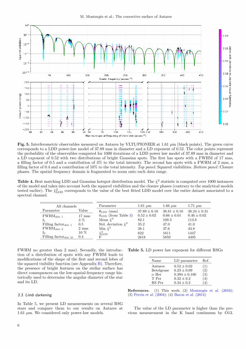
Fig. 5. Interferometric observables measured on Antares by VLTI/PIONIER at 1.61 µm (black points). The green curvecorresponds to a LDD power-law model of 37.89 mas in diameter and a LD exponent of 0.52. The color points representthe probability of the observables computed for 1000 iterations of a LDD power law model of 37.89 mas in diameter anda LD exponent of 0.52 with two distributions of bright Gaussian spots. The first has spots with a FWHM of 17 mas,a filling factor of 0.5 and a contribution of 3% to the total intensity. The second has spots with a FWHM of 2 mas, afilling factor of 0.4 and a contribution of 10% to the total intensity. Top panel: Squared visibilities. Bottom panel: Closurephases. The spatial frequency domain is fragmented to zoom onto each data range.

Table 4. Best matching LDD and Gaussian hotspot distribution model. The χ2 statistic is computed over 1000 instancesof the model and takes into account both the squared visibilities and the closure phases (contrary to the analytical modelstested earlier). The χ2

LDD corresponds to the value of the best fitted LDD model over the entire dataset associated to aspectral channel.

All channelsParameter ValueFWHMdist 1 17 masI1 3 %Filling factordist 1 0.5FWHMdist 2 2 masI2 10 %Filling factordist 21 0.4

Parameter 1.61 µm 1.66 µm 1.71 µmθLDD (mas) 37.89 ± 0.10 38.81 ± 0.10 38.24 ± 0.31δLDD (from Table 3) 0.52 ± 0.02 0.66 ± 0.01 0.46 ± 0.02Mean χ2 82.1 109.3 113.8Std. deviation χ2 35.2 47.0 41.0Min χ2 28.1 37.6 43.8χ2

LDD 622 1611 1447F 2818 5859 4495

FWHM no greater than 2 mas). Secondly, the introduc-tion of a distribution of spots with any FWHM leads tomodifications of the shape of the first and second lobes ofthe squared visibility function (see Appendix B). Therefore,the presence of bright features on the stellar surface hasdirect consequences on the low-spatial-frequency range his-torically used to determine the angular diameter of the starand its LD.

3.3. Limb darkening

In Table 5, we present LD measurements on several RSGstars and compare them to our results on Antares at1.61 µm. We considered only power-law models.

Table 5. LD power law exponent for different RSGs

Name LD parameter Ref.Antares 0.52 ± 0.02 (1)Betelgeuse 0.23 ± 0.09 (2)α Her 0.394 ± 0.180 (3)T Per 0.32 ± 0.2 (4)RS Per 0.34 ± 0.2 (4)

References. (1) This work; (2) Montarges et al. (2016);(3) Perrin et al. (2004); (4) Baron et al. (2014)

The value of the LD parameter is higher than the pre-vious measurement in the K band continuum by O13.

6

M. Montarges et al.: The convective surface of Antares

Although we have analyzed our dataset differently, wewould like to state that even by considering the whole spa-tial frequency range, we reach a LD parameter of ∼ 0.4;still higher than theirs. This makes it also higher than sim-ilar observations on other RSGs. However, as we have onlyone PA direction in the second lobe to constrain the LDmeasurement, we cannot exlude that this value is biasedby photospheric features.

4. Numerical approach: radiative hydrodynamicssimulation

To go beyond analytical models, we now turn to nu-merical convective simulations based on 3D radiativehydrodynamics computations. On Betelgeuse, C10b andMontarges et al. (2014) managed to reproduce the mea-sured squared visibilities with such numerical models.However, Montarges et al. (2016) did not reproduce boththe squared visibilities and the closure phases of their Hband PIONIER observations of the same star. They sug-gested that the convective activity was disturbed by thepresence of a large hot spot identified as the top of a hugeconvective cell.

To fit our PIONIER data of Antares, we used two sim-ulations obtained with the CO5BOLD code (COnservativeCOde for the COmputation of COmpressible COnvectionin a BOx of L Dimensions, L = 2, 3, Freytag et al. 2012),with stellar parameters close to those derived on Antares(O13). The characteristics of these numerical models aregiven in Table 6. We note that rotation is not yet imple-mented in these models. Computation of RHD models iscomplex and very demanding of computer resources, andit has not yet been possible to prepare a suite of modelsspecifically tuned to Antares. For now, we choose the bestavailable models, and leave for the future custom modelgeneration and iteration for each star studied.

We checked that we do not reach the numerical limit in-duced by the spatial gridding of the simulations. Accordingto Chiavassa et al. (2009, Eq.3), artifacts will affectthe derived visibilities for spatial frequencies higher than0.03 R−1

� . Using the equation:

ν[arcsec−1] = ν[R−1� ] · d[pc] · 214.9, (6)

we convert this to 1250 arcsec−1. We note that thedistance in parsec is not the actual distance between thesolar system and Antares but the distance required for thestellar model to have the same apparent angular size asAntares. Therefore, our VLTI/PIONIER data, althoughwith a very high resolution, are still below the frequencyof expected artifacts in the simulations.

For each simulation, hundreds of temporal snapshotswere computed; each of them is a realization of the con-vective pattern of the star. Using the 3D pure-LTE (lo-cal thermodynamical equilibrium) radiative transfer codeOptim3D (Chiavassa et al. 2009), intensity images are com-puted in the three spectral channels of our PIONIER obser-vations. As Antares may have any orientation on the planeof the sky relative to the simulation, we rotated each imagearound its center. We used 36 angle positions between 0◦

and 180◦. The distance of Antares was taken into accountby scaling the angular diameters to the value we derived

from the LD power law. Interferometric observables werecomputed using a Fast Fourier Transform algorithm.

Contrary to previous matches of interferometric datawith these simulations (C10b, Chiavassa et al. 2010c,Montarges et al. 2014, 2016 or Arroyo-Torres et al. 2015), we did not seek the best matching snapshot and rotationangle. Instead, we considered the χ2 associated to the wholegrid of temporal snapshots and rotation angles for bothsimulations. The characteristics of these χ2 distributionsare given in Table 7. The closure phases are mostly con-strained by positional information of the inhomogeneities.Therefore, we only considered the squared visibilities thatgive mainly information about the number and size of thestellar features.

The simulation st35gm03n13 gives a better match to theobserved squared visibilities. It has a non-gray opacity ap-proximation (we refer to C11a for the details about thisphysical approximation). This causes an intensified heatexchange of a fluid element with its environment, reduc-ing the temperature/density fluctuations (Fig. 5 in C11a).Less intense fluctuations reduce the surface intensity con-trast of nearby areas and, eventually, interferometric ob-servables. On the contrary, the st35g03n07 simulation hasa gray opacity approximation.

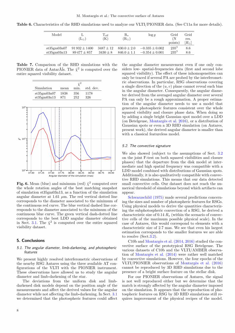
We saw in Sect. 3 that the angular diameter determi-nation is strongly sensitive to the presence of stellar fea-tures as they may directly affect the squared visibilities inthe first lobe. Thus, for the best matching temporal snap-shot of the best simulation, we generated squared visibili-ties matching our PIONIER observations for a stellar modelbetween 37.0 and 39.0 mas with a step of 0.1 mas, and wekept the 36 rotation angles. The mean and minimum χ2 arerepresented on Fig. 6. It appears that the χ2 value stronglydepends on the fixed angular diameter of the simulation. Inparticular, the simulations computed with the best LDD di-ameter (38.24 ± 0.37 mas) derived in Sect. 3.1 do not givethe best result. The minimum χ2 of 182.2 is reached foran angular diameter of 37.60 ± 0.08 mas at 1.61 µm. Thissmaller size between the 3D simulations and the classicalangular diameter fit of interferometric data is consistentwith previous results from Chiavassa et al. (2010a) thatnoted a similar discrepancy with K giant observations. Themain origin would be the presence of bright inhomogeneitiesthat force a smaller angular diameter in order to keep thesame integrated luminosity over the stellar disk.

However, this χ2 , computed over the squared visibilitiesonly, remains worse than what is achievable with the powerlaw LDD alone (∼ 25 for the whole squared visibility data inSect. 3.1) or the random distribution of Gaussian spots (∼28− 44 in Sect. 3.2 for both closure phases and visibilities,that should be in principle more difficult to fit). This is alsowhat was obtained on the RSG Betelgeuse (Montarges et al.2016). This comes as a surprise as previous interferometricobservations in the H (C10b) and K bands (Montarges et al.2014) were well matched by 3D RHD simulations. It is notwithin the scope of this paper to study the quality of thematch between observations and simulations over time forRSG stars but we would like to stress the importance ofcontinuous monitoring of these stars over time with variousinterferometric instruments. Their convective patterns donot appear to be always reproducible by current state-of-the-art RHD simulations.

7

M. Montarges et al.: The convective surface of Antares

Table 6. Characteristics of the RHD simulations used to analyze our VLTI/PIONIER data. (See C11a for more details).

Model L Teff R? log g Grid Grid(L�) (K) (R�) (N res.

points) [R�]st35gm03n07 91 932 ± 1400 3487 ± 12 830.0 ± 2.0 −0.335 ± 0.002 2353 8.6st35gm03n13 89 477 ± 857 3430 ± 8 846.0 ± 1.1 −0.354 ± 0.001 2353 8.6

Table 7. Comparison of the RHD simulations with thePIONIER data of AntarÃĺs. The χ2 is computed over theentire squared visibility dataset.

χ2

Simulation mean min. std. dev.st35gm03n07 1838 356 1178st35gm03n13 871 252 326

37.00 37.25 37.50 37.75 38.00 38.25 38.50 38.75 39.00Angular diameter of the simulation (mas)

102

103

104

2

Fig. 6. Mean (blue) and minimum (red) χ2 computed overthe whole rotation angles of the best matching snapshotof simulation st35gm03n13, as a function of the simulationangular diameter at 1.61 µm. The red vertical dotted linecorresponds to the diameter associated to the minimum ofthe continuous red curve. The blue vertical dashed line cor-responds to the diameter associated to the minimum of thecontinuous blue curve. The green vertical dash-dotted linecorresponds to the best LDD angular diameter obtainedin Sect. 3.1. The χ2 is computed over the entire squaredvisibility dataset.

5. Conclusions5.1. The angular diameter, limb-darkening, and photospheric

features

We present highly resolved interferometric observations ofthe nearby RSG Antares using the three available AT con-figurations of the VLTI with the PIONIER instrument.These observations have allowed us to study the angulardiameter and limb-darkening of the star.

The deviations from the uniform disk and limb-darkened disk models depend on the position angle of themeasurements and affect the derived values for the angulardiameter while not affecting the limb-darkening. In Sect. 3.1we determined that the photospheric features could affect

the angular diameter measurement even if one only con-siders low- spatial-frequencies data (first and second lobesquared visibility). The effect of these inhomogeneities canonly be traced if several PA are probed by the interferomet-ric observations. In particular, RSG observations coveringa single direction of the (u, v) plane cannot reveal such biasin the angular diameter. Consequently, the angular diame-ter derived from the averaged angular diameter over severalPA can only be a rough approximation. A proper estima-tion of the angular diameter needs to use a model thatgenerates photospheric features consistent over the wholesquared visibility and closure phase data. When doing soby adding a single bright Gaussian spot model over a LDD(on Betelgeuse, Montarges et al. 2016), or a distribution ofGaussian spots or even a 3D RHD simulation (on Antares,present work), the derived angular diameter is smaller thanwith a classical featureless model.

5.2. The convective signature

We also showed (subject to the assumptions of Sect. 3.2on the joint F-test on both squared visibilities and closurephases) that the departure from the disk model at inter-mediate and high spatial frequency was compatible with aLDD model combined with distributions of Gaussian spots.Additionally, it is also qualitatively compatible with convec-tive RHD simulations. This means that our data detectedsmall convective cells. Our dataset does not reach the nu-merical threshold of simulations beyond which artifacts canappear.

Schwarzschild (1975) made several predictions concern-ing the sizes and number of photospheric features for RSGs.Using physical models to derive the quantities characteriz-ing the subphotospheric convection of a RSG, he derived acharacteristic size of 0.14 R? (within the scenario of convec-tive cells of the maximum possible physical scale). In thecase of Antares, this would correspond to elements with acharacteristic size of 2.7 mas. We see that even his largestestimation corresponds to the smaller features we are ableto resolve (Sect.3.2).

C10b and Montarges et al. (2014, 2016) studied the con-vective surface of the prototypical RSG Betelgeuse. Thevarious datasets of C10b and the VLTI/AMBER observa-tion of Montarges et al. (2014) were rather well matchedby convective simulations. However, the four epochs of theVLTI/PIONIER observations of Montarges et al. (2016)cannot be reproduced by 3D RHD simulations due to thepresence of a bright surface feature on the stellar disk.

For our PIONIER observations of Antares, the signalis not well reproduced either but we determine that thematch is strongly affected by the angular diameter imposedon the simulation. It appears that the reproduction of pho-tospheric features on RSG by 3D RHD simulations still re-quires improvement of the physical recipes of the model.

8

M. Montarges et al.: The convective surface of Antares

Temporal monitoring at different wavelengths of severalRSG stars would help constrain those missing ingredientsby providing more examples of convective patterns.

Acknowledgements. We are grateful to the Paranal Observatory teamfor the successful execution of the observations. This research re-ceived the support of PHASE, the high angular resolution partner-ship between ONERA, Observatoire de Paris, CNRS and UniversityDenis Diderot Paris 7. We acknowledge financial support from the“Programme National de Physique Stellaire” (PNPS) of CNRS/INSU,France. The authors would like to thank Alain Chelli for his useful ad-vice on the handling of closure phases and squared visibilities from astatistical point of view. We used the SIMBAD and VIZIER databasesat the CDS, Strasbourg (France)3, and NASA’s Astrophysics DataSystem Bibliographic Services. This research has made use of Jean-Marie Mariotti Center’s Aspro4 service, of the LITpro5 software (co-developped by CRAL, LAOG and FIZEAU) and of the SearchCalservice6 (co-developped by FIZEAU and LAOG/IPAG). This re-search made use of IPython (Perez & Granger 2007) and Astropy7, acommunity-developed core Python package for Astronomy (AstropyCollaboration et al. 2013).

ReferencesArroyo-Torres, B., Wittkowski, M., Chiavassa, A., et al. 2015, A&A,

575, A50Astropy Collaboration, Robitaille, T. P., Tollerud, E. J., et al. 2013,

A&A, 558, A33Baron, F., Monnier, J. D., Kiss, L. L., et al. 2014, ApJ, 785, 46Bonneau, D., Clausse, J.-M., Delfosse, X., et al. 2006, A&A, 456, 789Bonneau, D., Delfosse, X., Mourard, D., et al. 2011, A&A, 535, A53Chiavassa, A., Collet, R., Casagrande, L., & Asplund, M. 2010a, A&A,

524, A93Chiavassa, A., Freytag, B., Masseron, T., & Plez, B. 2011, A&A, 535,

A22Chiavassa, A., Haubois, X., Young, J. S., et al. 2010b, A&A, 515, A12Chiavassa, A., Lacour, S., Millour, F., et al. 2010c, A&A, 511, A51Chiavassa, A., Plez, B., Josselin, E., & Freytag, B. 2009, A&A, 506,

1351Freytag, B., Steffen, M., Ludwig, H.-G., et al. 2012, Journal of

Computational Physics, 231, 919Gray, D. F. 2008, The Observation and Analysis of Stellar

PhotospheresHaguenauer, P., Alonso, J., Bourget, P., et al. 2010, in Society

of Photo-Optical Instrumentation Engineers (SPIE) ConferenceSeries, Vol. 7734

Hanbury Brown, R., Davis, J., Lake, R. J. W., & Thompson, R. J.1974, MNRAS, 167, 475

Harper, G. M. 2010, in Astronomical Society of the Pacific ConferenceSeries, Vol. 425, Hot and Cool: Bridging Gaps in Massive StarEvolution, ed. C. Leitherer, P. D. Bennett, P. W. Morris, & J. T.Van Loon, 152

Haubois, X., Perrin, G., Lacour, S., et al. 2009, A&A, 508, 923Hestroffer, D. 1997, A&A, 327, 199Josselin, E. & Plez, B. 2007, A&A, 469, 671Le Bouquin, J.-B., Berger, J.-P., Lazareff, B., et al. 2011, A&A, 535,

A67Merand, A., Borde, P., & Coude du Foresto, V. 2005, A&A, 433, 1155Montarges, M., Kervella, P., Perrin, G., et al. 2016, A&A, 588, A130Montarges, M., Kervella, P., Perrin, G., et al. 2014, A&A, 572, A17Ohnaka, K. 2014, A&A, 568, A17Ohnaka, K., Hofmann, K.-H., Schertl, D., et al. 2013, A&A, 555, A24Perez, F. & Granger, B. E. 2007, Computing in Science and

Engineering, 9, 21Perrin, G., Ridgway, S. T., Coude du Foresto, V., et al. 2004, A&A,

418, 675Pugh, T. & Gray, D. F. 2013, ApJ, 777, 10Rayner, J. T., Cushing, M. C., & Vacca, W. D. 2009, ApJS, 185, 289Schwarzschild, M. 1975, ApJ, 195, 137

3 Available at http://cdsweb.u-strasbg.fr/4 Available at http://www.jmmc.fr/aspro5 Available at http://www.jmmc.fr/litpro6 Available at http://www.jmmc.fr/searchcal7 Available at http://www.astropy.org/

Stothers, R. B. 2010, ApJ, 725, 1170van Leeuwen, F. 2007, A&A, 474, 653

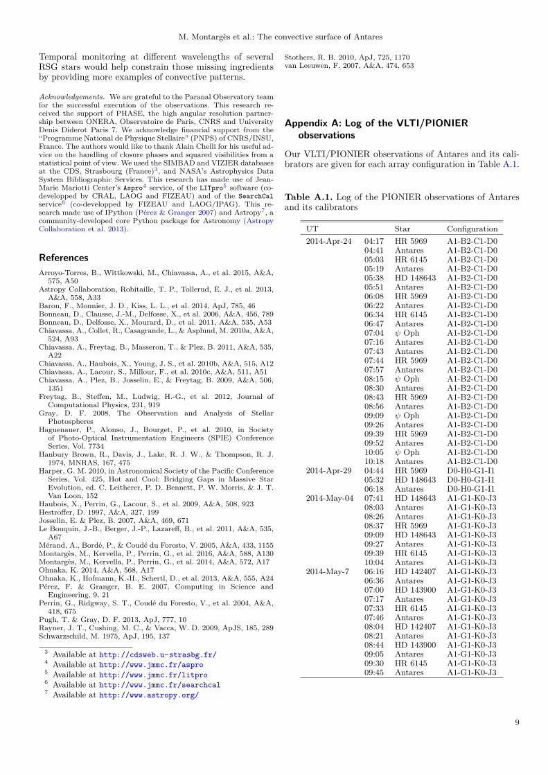
Appendix A: Log of the VLTI/PIONIERobservations

Our VLTI/PIONIER observations of Antares and its cali-brators are given for each array configuration in Table A.1.

Table A.1. Log of the PIONIER observations of Antaresand its calibrators

UT Star Configuration2014-Apr-24 04:17 HR 5969 A1-B2-C1-D0

04:41 Antares A1-B2-C1-D005:03 HR 6145 A1-B2-C1-D005:19 Antares A1-B2-C1-D005:38 HD 148643 A1-B2-C1-D005:51 Antares A1-B2-C1-D006:08 HR 5969 A1-B2-C1-D006:22 Antares A1-B2-C1-D006:34 HR 6145 A1-B2-C1-D006:47 Antares A1-B2-C1-D007:04 ψ Oph A1-B2-C1-D007:16 Antares A1-B2-C1-D007:43 Antares A1-B2-C1-D007:44 HR 5969 A1-B2-C1-D007:57 Antares A1-B2-C1-D008:15 ψ Oph A1-B2-C1-D008:30 Antares A1-B2-C1-D008:43 HR 5969 A1-B2-C1-D008:56 Antares A1-B2-C1-D009:09 ψ Oph A1-B2-C1-D009:26 Antares A1-B2-C1-D009:39 HR 5969 A1-B2-C1-D009:52 Antares A1-B2-C1-D010:05 ψ Oph A1-B2-C1-D010:18 Antares A1-B2-C1-D0

2014-Apr-29 04:44 HR 5969 D0-H0-G1-I105:32 HD 148643 D0-H0-G1-I106:18 Antares D0-H0-G1-I1

2014-May-04 07:41 HD 148643 A1-G1-K0-J308:03 Antares A1-G1-K0-J308:26 Antares A1-G1-K0-J308:37 HR 5969 A1-G1-K0-J309:09 HD 148643 A1-G1-K0-J309:27 Antares A1-G1-K0-J309:39 HR 6145 A1-G1-K0-J310:04 Antares A1-G1-K0-J3

2014-May-7 06:16 HD 142407 A1-G1-K0-J306:36 Antares A1-G1-K0-J307:00 HD 143900 A1-G1-K0-J307:17 Antares A1-G1-K0-J307:33 HR 6145 A1-G1-K0-J307:46 Antares A1-G1-K0-J308:04 HD 142407 A1-G1-K0-J308:21 Antares A1-G1-K0-J308:44 HD 143900 A1-G1-K0-J309:05 Antares A1-G1-K0-J309:30 HR 6145 A1-G1-K0-J309:45 Antares A1-G1-K0-J3

9

M. Montarges et al.: The convective surface of Antares

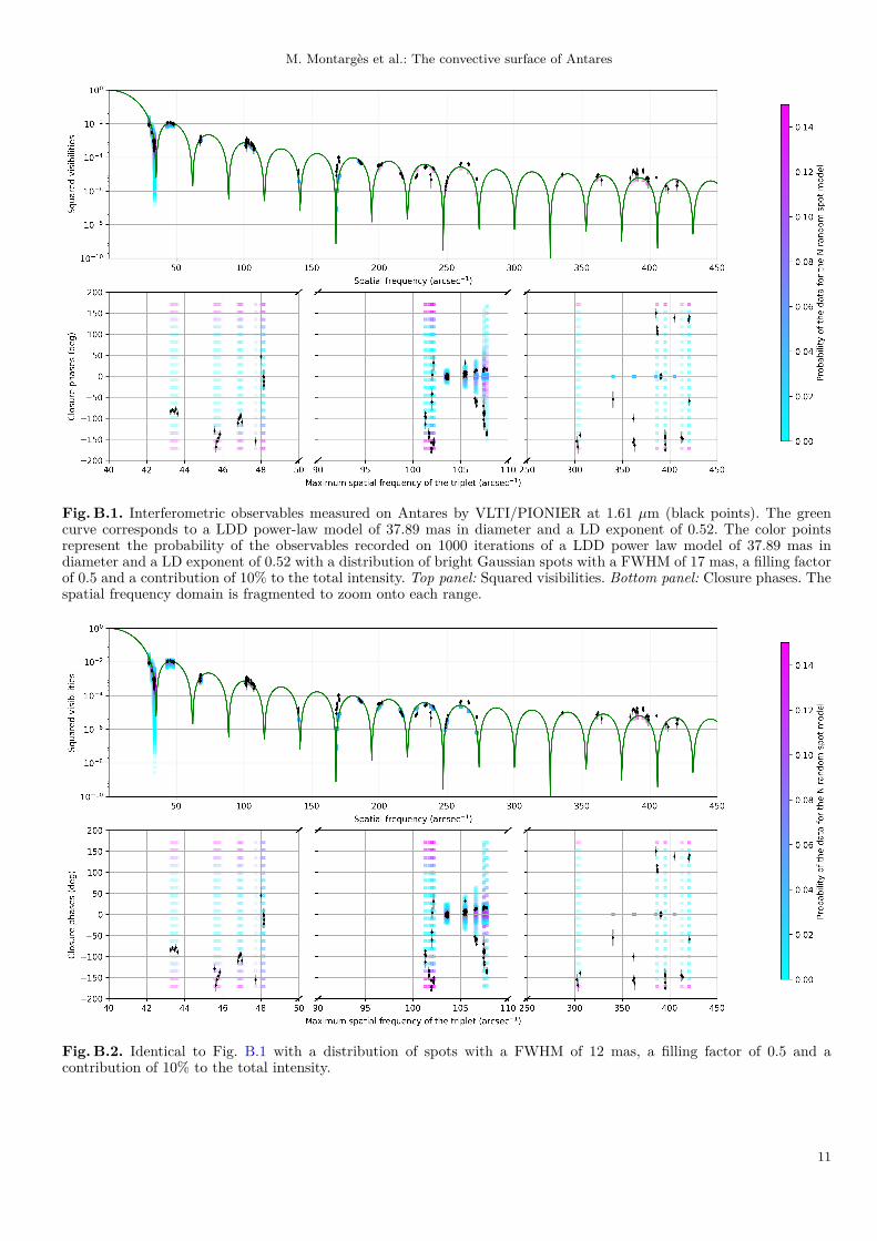
Appendix B: Example of random Gaussian spotdistribution in a limb-darkened disk

To obtain more details on the model used in the followingexamples, we refer the reader to Sect. 3.2. The example arepresented in Figs. B.1, B.2, B.3 and B.4.

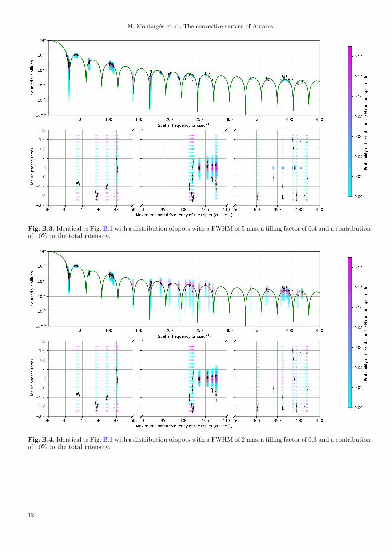
The decreasing size of the bright Gaussian spots cre-ates more dispersion of the squared visibilities at higherand higher spatial frequencies and also increases the clo-sure phase signal (deviation from 0◦ or 180◦).

Appendix C: F-test to determine the significanceof the limb-darkening disk and Gaussian spotdistribution model fit on the squared visibilities

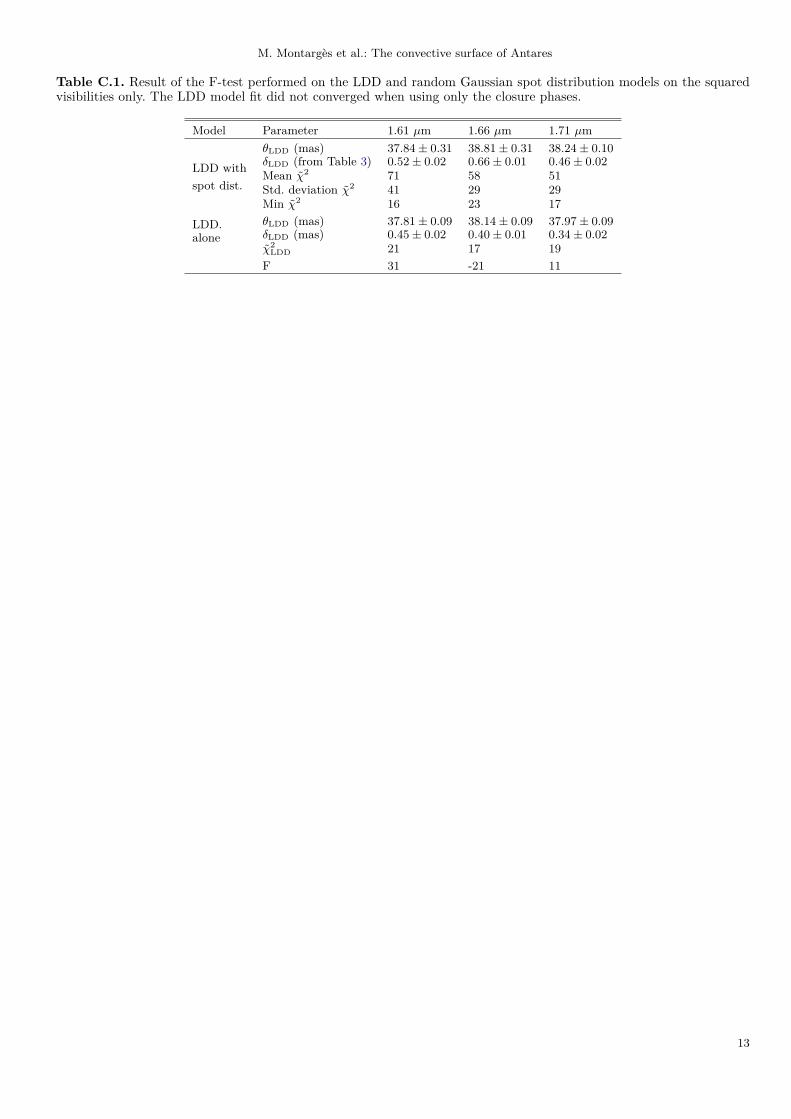
We performed an F-test to determine if the better matchof the spot distribution model is significant with respectto the null hypothesis (classical LDD). The F parameterexpression is given in Eq. 5. We tried to perform the testseparately on the squared visibilities and closure phases.However, it was impossible to make the LDD model (with-out spots) fit to converge with the closure phases only.Therefore, we only present the F-test on the squared vis-ibilities. The critical value for a (2, 5) F distribution8 is5.143. Therefore, from the values of Table C.1, our modelfitting with bright spots is significant only in the first andthird spectral channels of our VLTI/PIONIER squared vis-ibilities. This could mean that at 1.66 µm the features areless prominent but this is without taking into account theclosure phase signal. In Sect. 3.2, we present the fit on boththe squared visibilities and closure phases with a F factormuch higher, meaning that the closure phases bring infor-mation about the asymmetries that are reproduced by ourmodel.

8 http://www.itl.nist.gov/div898/handbook/eda/section3/eda3673.htm

10

M. Montarges et al.: The convective surface of Antares

Fig. B.1. Interferometric observables measured on Antares by VLTI/PIONIER at 1.61 µm (black points). The greencurve corresponds to a LDD power-law model of 37.89 mas in diameter and a LD exponent of 0.52. The color pointsrepresent the probability of the observables recorded on 1000 iterations of a LDD power law model of 37.89 mas indiameter and a LD exponent of 0.52 with a distribution of bright Gaussian spots with a FWHM of 17 mas, a filling factorof 0.5 and a contribution of 10% to the total intensity. Top panel: Squared visibilities. Bottom panel: Closure phases. Thespatial frequency domain is fragmented to zoom onto each range.

Fig. B.2. Identical to Fig. B.1 with a distribution of spots with a FWHM of 12 mas, a filling factor of 0.5 and acontribution of 10% to the total intensity.

11

M. Montarges et al.: The convective surface of Antares

Fig. B.3. Identical to Fig. B.1 with a distribution of spots with a FWHM of 5 mas, a filling factor of 0.4 and a contributionof 10% to the total intensity.

Fig. B.4. Identical to Fig. B.1 with a distribution of spots with a FWHM of 2 mas, a filling factor of 0.3 and a contributionof 10% to the total intensity.

12

M. Montarges et al.: The convective surface of Antares

Table C.1. Result of the F-test performed on the LDD and random Gaussian spot distribution models on the squaredvisibilities only. The LDD model fit did not converged when using only the closure phases.

Model Parameter 1.61 µm 1.66 µm 1.71 µmθLDD (mas) 37.84 ± 0.31 38.81 ± 0.31 38.24 ± 0.10

LDD with δLDD (from Table 3) 0.52 ± 0.02 0.66 ± 0.01 0.46 ± 0.02

spot dist.Mean χ2 71 58 51Std. deviation χ2 41 29 29Min χ2 16 23 17

LDD. θLDD (mas) 37.81 ± 0.09 38.14 ± 0.09 37.97 ± 0.09alone δLDD (mas) 0.45 ± 0.02 0.40 ± 0.01 0.34 ± 0.02

χ2LDD 21 17 19

F 31 -21 11

13