VLV RI PLWLJDWLRQ PHDVXUHV RQ XUEDQ DUWHULDOV …

European Transport \ Trasporti Europei (2021) Issue 81, Paper n° 7, ISSN 1825-3997

https://doi.org/10.48295/ET.2021.81.7

Development of congestion index model and analysis of mitigation measures on urban arterials using

microsimulation

Akshara S.1, S. Marisamynathan2

1Postgraduate student, Department of Civil Engineering, National Institute of Technology Tiruchirappalli, Tamil Nadu – 620015, India

2Assitant Professor, National Institute of Technology Tiruchirappalli, Tamil Nadu – 620015, India Abstract Traffic congestion is one of the main issues related to traffic engineering, planning, and policies that directly influence the economy, environment, and lifestyle in developing countries, particularly in India. This study's main objectives are to establish the congestion index model and analyze the various mitigation measures using microsimulation. The required data were collected from selected two corridors in Tiruchirappalli, India. A correlation test was performed to identify the significant parameters that influence traffic congestion. Congestion Indices and Travel time reliability measures were computed to quantify congestion. Using a conventional regression technique, the congestion index model was developed to predict the congestion levels. The validated model predicts the congestion accurately. The mentioned statistical tests and model development were performed in SPSS 25.0 software at 95% confidence interval. A VISSIM based microsimulation was calibrated and simulated various mitigation measures with possible scenarios. Thus, the mind-numbing traffic jams can be reduced, and as a result, a great loss for the Indian economy can be reduced. Keywords: Congestion, Regression Analysis, Speed Reduction Index, Microsimulation, VISSIM.

1. Introduction

Transportation network plays the key role on urban activities. Due to increased population and various land-use activities, the transportation system requires major updates or readjustments. Traffic congestion leads to time loss, environmental pollution, and economic loss on society. Congestion creates both quantifiable and unquantifiable costs for individual road users and society. Due to variation in daily traffic supply and demand, any city transportation system network faces imbalanced conditions. Thus, congestion is one of the main pre-occupation of transport decision-makers. Congestion occurs when the demand goes beyond the transportation network system capacity. Congestion creates a greater impact on the travel speed and time of individual users. Travel time, travel speed, and delay are the primary measures that are used to quantify congestion. These measures are considered travel time-based measures and they are more flexible to define traffic conditions with various levels in both space and time. The volume

Corresponding author: Akshara S ([email protected])


2

to capacity ratio is considered an alternative measure to define travel time reliability, which can help estimate the adequacy of the service provided in the transportation network. With the increase in travel demand, congestion has been established as an inescapable reality of urban life. From the road user’s perspective, they expect that the road network should meet the higher requirements on the level of services, instead of travel demand. Thus, establishing a clear, timely, and efficient road network system is a suitable solution for this congestion problem. To improve the mobility and operational efficiency of the road network, the existing network efficiency is to be found. For this purpose of quantifying congestion, various congestion indices have been advocated, which is a measure of roadway service quality. Therefore, this study aims to identify the various matrices to quantify congestion and develop a Congestion Index Model concerning the speed with speed reduction index as the dependent variable.

2. Literature Review

Congestion can be defined as the state of high densities and low speeds in a given corridor (Bovy and Salomon, 2002). Many studies described congestion as traffic delay (Weisbrod et al., 2001), excess travel time (Lomax et al., 1997), and immobility (Levinson and Lomax 1996). Boarnet et al. (1998) suggested the various issues on network performance which is to be addressed while measuring congestion. Turner (1992) studied indicators of congestion and suggested measures to quantify the level of congestion. Medley and Demetsky (2003) examined congestion with respect to total delay and buffer index. Stathopoulos and Karlaftis (2002) developed the log-logistic function to estimate the duration of congestion on a given road stretch. Most of the studies adopted recurrent and non-recurrent congestion (Dowling et al. (2004)), (Skabardonis et al., (2003)), judgmental model (Ishida et al. (2003)), regression model (Cottrell (1991)), fuzzy model (Hamad and Kikuchi 2002) and simulation program (Dewees (1978), G Gomez et al., (2004), Cardenas et al., (2018), Akbar et al., (2018)) for estimating the congestion level in a given corridor.

Sruthy Henry and Bino I Koshy (2016) stated that congestion reduces residents' effective accessibility, resulting in lost opportunities for both the public and business. S. Vasantha Kumar and R.Sivanandan (2012) proved that travel-time based congestion quantification delivers more advantages compared with other approaches. Aachal Dhote et al., (2017) stated that traffic congestion occurs when traffic volume generates demand for space greater than the available road capacity i.e. when demand approaches the capacity of the road.

Krishna Saw et al., (2016) developed a travel speed index to evaluate congestion and developed a multiple linear regression model to model congestion. M.V.L.R. Anjaneyulu and B.N. Nagaraj (2009) have provided a new approach that considered the speed variations as the basis for estimating congestion and improving the level of service. A microscopic simulation tool was used for evaluating the congestion mitigation alternatives and their performance before implementing for the existing traffic conditions (Amudapuram Mohan Rao and K. Ramachandra, 2016). Dewan and Ahmad (2007) suggested a car-pooling system for reducing congestion in Delhi, and found the willingness of road used to shift car-pooling system from individual vehicles.

The literature review has revealed that the fluctuations in speed, which is the most primary effect of congestion, have not yet been utilized for congestion modeling under heterogeneous traffic conditions, particularly in India. Most of the existing studies focused on volume to capacity ratios and level of service measurements to estimate the


3

travel condition. Existing models on congestion prediction fail to predict the congestion for Indian conditions due to mixed traffic conditions and different road user behaviors. This study attempts to provide an alternative methodology for congestion model development in terms of speed and travel time and identify the various possible mitigation measures using calibrated microsimulation model.

3. Research Objectives

The objectives of this study are as follows: (a) to analyze the traffic congestion on the urban road network and understand the various parameters involved in it; (b) to quantify congestion using different congestion indices and to evaluate travel time reliability measures; (c) to develop congestion index model to predict the level of congestion on the selected corridors; and (d) to prioritize the selected mitigation measures by performing micro-simulation analysis.

4. Study Sites

The prime focus of this study lies in the urban arterials of Tiruchirappalli, Tamil Nadu, India. The road stretches taken into consideration were Gandhi Market Road of about 1.42 km and Palakkarai Road of about 500 m, as shown in Figure 1. Gandhi Market road is a busy commercial road stretch, the heart of the city along which most of the buses connecting Thanjavur and Chatram ply. Palakkarai is one of the primary residential and densely populated areas.

Figure 1: Study stretch for the congestion analysis in Gandhi market and Palakkarai (54 m trap length)

In both the study locations, there were no proper pavement markings and illegal on street parking was observed on either sides of the road stretches. The illegal parking on either side of the road stretch was using the existing pavement, limiting the space available and thereby leading to congestion.

5. Data Collection

Before the data collection process, a site investigation survey was conducted to determine the study stretch suitability. Initially, the possible road sections were selected using Google Map. Site investigations were performed to estimate the potentiality of study segments. The details of the selected study stretches are presented in Table 1.

Traffic data was collected during peak hours and off-peak hours by videographic survey on weekdays. During the study, six categories of vehicles were identified such as Bus, Two-wheeler (TW), Car, Light Commercial Vehicle (LCV), Heavy Commercial Vehicle


4

(HCV), and Auto rickshaw. A parking survey was also carried out in both locations to study parked vehicles influence on the street to the moving traffic.

Table 1 Details of the selected study stretches Sl

No. Name of the road

Class of road

Lane characteristics Length (m) Land use pattern

1 Gandhi Market Arterial Two-lane undivided 1420 Commercial area 2 Palakkarai Arterial Two-lane undivided 500 Commercial area

6. Data Extraction and Analysis

6.1. Data Extraction

The required data was extracted from the collected video using Traffic Data Extractor (TDE). It is used to obtain the volume count, vehicle speed, and vehicle trajectory separately for two directions from each road network. The extraction of the data was extremely time-consuming as the video was played very slowly.

Another parameter extracted from the video was the number of pedestrians crossing the street at every 5-minute interval. The stretch's geometric details were obtained from the field by means of a measuring tape as shown in Table 2. Dwelling time of bus was obtained from the field using the stopwatch.

Table 2 Geometric details of the selected corridors Location ID Name of the road Length (m) Trap length (m) Width (m)

1 Gandhi market 1420 54 7.5 2 Palakkarai 500 54 8

6.2. Traffic Volume Analysis

Traffic volume count results give a measure of comparison of heterogeneous traffic on the selected study stretch. Volume count was done at an interval of 5 minutes for each category of vehicles from the video. The volume count was computed in vehicles/hr, and it was converted to PCU/hr using the conversion factors provided by Indo-HCM. The results are tabulated in Table 3.

Table 3 Traffic volume counts on the selected road stretch

Table 3 presents the traffic volume count on Gandhi Market and Palakkarai in both directions separately. The traffic characteristics of the roads are changing as years are passing mainly due to change in pricing of vehicles and change in the economy. The vehicle ownership levels are increasing tremendously. The traffic composition for the selected two roads was picturized in Figures 2 and 3.

Location Id

Road Name Direction Peak Volume (PCU / hr)

From To Up Down 1 Gandhi Market road Palpannai Chatram Market 2142 1987 2 Palakkarai Junction Chatram 2184 2006


5

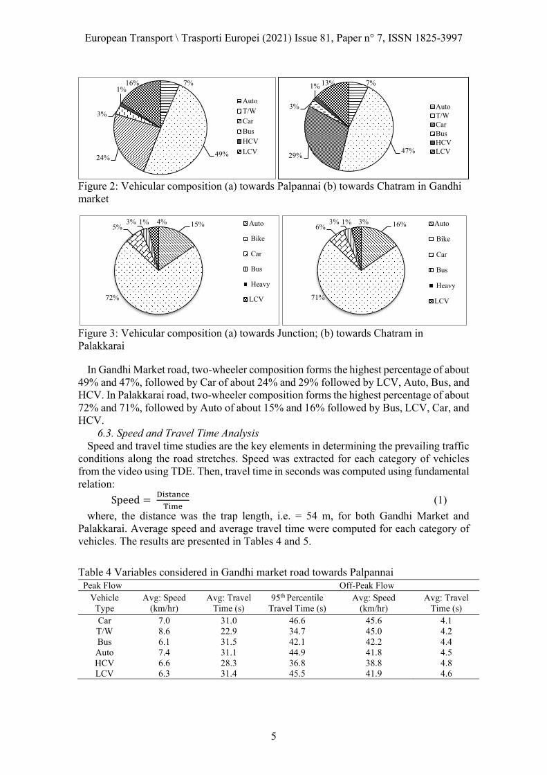
Figure 2: Vehicular composition (a) towards Palpannai (b) towards Chatram in Gandhi market

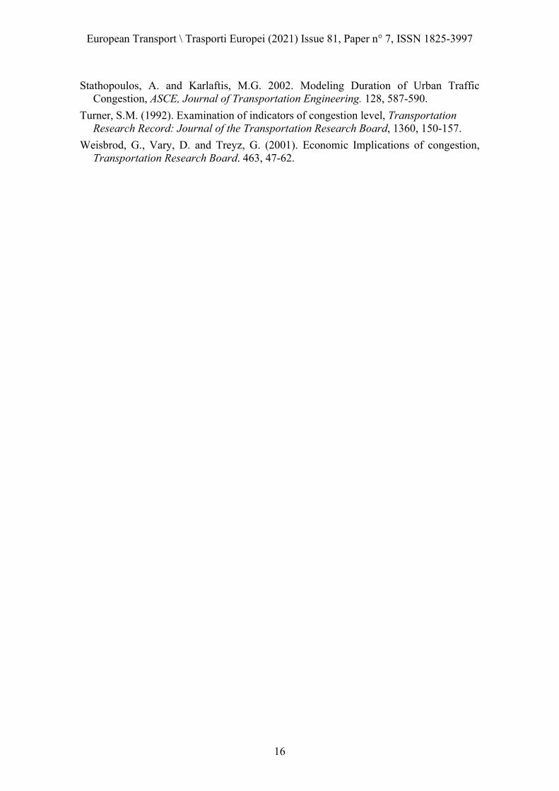
Figure 3: Vehicular composition (a) towards Junction; (b) towards Chatram in Palakkarai

In Gandhi Market road, two-wheeler composition forms the highest percentage of about 49% and 47%, followed by Car of about 24% and 29% followed by LCV, Auto, Bus, and HCV. In Palakkarai road, two-wheeler composition forms the highest percentage of about 72% and 71%, followed by Auto of about 15% and 16% followed by Bus, LCV, Car, and HCV.

6.3. Speed and Travel Time Analysis Speed and travel time studies are the key elements in determining the prevailing traffic

conditions along the road stretches. Speed was extracted for each category of vehicles from the video using TDE. Then, travel time in seconds was computed using fundamental relation:

Speed = (1)

where, the distance was the trap length, i.e. = 54 m, for both Gandhi Market and Palakkarai. Average speed and average travel time were computed for each category of vehicles. The results are presented in Tables 4 and 5.

Table 4 Variables considered in Gandhi market road towards Palpannai

7%

49%24%

3%

1%16%

AutoT/WCarBusHCVLCV

7%

47%29%

3%

1% 13%

AutoT/WCarBusHCVLCV

15%

72%

5%3% 1% 4% Auto

Bike

Car

Bus

Heavy

LCV

16%

71%

6%3% 1% 3% Auto

Bike

Car

Bus

Heavy

LCV

Peak Flow Off-Peak Flow Vehicle

Type Avg: Speed

(km/hr) Avg: Travel

Time (s) 95th Percentile

Travel Time (s) Avg: Speed

(km/hr) Avg: Travel

Time (s) Car 7.0 31.0 46.6 45.6 4.1 T/W 8.6 22.9 34.7 45.0 4.2 Bus 6.1 31.5 42.1 42.2 4.4 Auto 7.4 31.1 44.9 41.8 4.5 HCV 6.6 28.3 36.8 38.8 4.8 LCV 6.3 31.4 45.5 41.9 4.6


6

Table 5 Variables considered in Gandhi market road towards Chatram Peak Flow Off-Peak Flow

Vehicle Type

Avg: Speed (km/hr)

Avg: Travel Time (s)

95th Percentile Travel Time (s)

Avg: Speed (km/hr)


Car 7.8 23.5 45.2 45.9 4.1 T/W 9.1 18.1 34.6 43.3 4.4 Bus 7.4 21.7 35.3 42.3 4.4 Auto 8.5 20.6 38.2 39.3 4.8 HCV 7.3 21.1 35.1 39.3 4.7 LCV 7.0 24.6 43.1 43.0 4.3

From Table 4 and Table 5, the speed during peak and off-peak flow towards Palpannai and Chatram in Gandhi market road, it is clear that the speed during peak flow was much less than that during free flow, i.e., the flow during peak hours was jammed. Thus, the stretch under consideration, i.e., Gandhi market road stretch, is under severe congestion.

Table 6 Variables considered in Palakkarai towards Chatram Peak Flow Off-Peak Flow

Vehicle Type

Avg: Speed (km/hr)



Avg: Speed (km/hr)



Table 7 Variables considered in Palakkarai towards Junction Peak Flow Off-Peak Flow

Vehicle Type

Avg: Speed (km/hr)



Avg: Speed (km/hr)



From Table 6 and Table 7, the speed during peak and off-peak flow towards Chatram and Junction respectively in Palakkarai, it is clear that speed during peak flow is much less than that during free flow, i.e., the flow during peak hours is jammed. Parameters that are evaluated from the data collected for computing the various congestion indices were average speed, average travel time, and 95th percentile travel time during peak flow, average speed, and average travel time during free flow.

7. Measures to Quantify Congestion

Congestion indices are used to measure the mobility and operational efficiency of the given road network system. Different types of indices used to measure the efficiency, speed reduction index, congestion index, and travel time reliability measures can produce more accurate results of existing conditions of road network system.


7

7.1 Speed Reduction Index (SRI)

SRI is a measure to denote the ratio of the reduction in speeds compared with free-flow conditions. SRI is computed using the following equation for each class of vehicle.

SRI = 1 −

∗ 10 (1)

If SRI is more than 4, it implies that the road stretch under consideration is congested.

7.2 Congestion Index (CI)

Travel time in peak and off-peak is compared using CI and is computed by using the following equation.

CI =

(2)

A value of 0 indicates a very low level of congestion, and a value greater than or equal to 2 corresponds to a very congested condition.

7.3 Travel Time Reliability Measures

Travel time reliability measures are used for evaluating existing measures of congestion in the transportation system. The three recommended measures used in this study such as Travel Time Index (TTI), Planning Time Index (PTI), and Buffer Index (BI).

7.4 Buffer Index (BI)

The BI represents the extra buffer time, which adds to most travelers’ average travel time when they target for on-time arrival. The BI is denoted by percentage. In this study, the BI were estimated using

BI =

(3)

7.5 Planning Time Index (PTI)

The PTI indicates the total travel time of individuals, which includes all buffer time in their journey. In this study, PTI is estimated using

PTI =

(4)

7.6 Travel Time Index (TTI)

TTI is the ratio between average travel time of peak hours and off-peak hour travel time. It is estimated as follows:

TTI =

(5)

Using equations 1 to 5, various congestion indices were computed and tabulated in Tables 8 to 11. Table 8 and 9 show that SRI value was greater than 4 and CI was greater than 2, towards Chatram and towards Palpannai, thus the selected corridors were congested. In Market road towards Chatram, PTI value of 8 indicates that 8 times of average travel time one has to plan as the total travel time while planning in the market road towards Palpannai. BI value of 0.71 indicates that 0.71 times of average travel time is the extra time one has to consider so as to reach the destination on time. In Market road towards Palpannai, TTI value of 7.5 indicates that the average travel time during peak hours is 7.5 times of average free-flow travel time.

Table 10 and 11 show that SRI value is greater than 4 and CI is greater than 2, towards Chatram and towards Palpannai, thus the selected corridor is congested. In Palakkarai towards Chatram, PTI value of 9.9 indicates that 9.9 times of average travel time one has


8

to plan as the total travel time while planning in Palakkarai towards Junction. BI value of 0.71 indicates that 0.71 times of average travel time is the extra time one has to consider so as to reach the destination on time. In Palakkarai towards Junction. TTI value of 3.9 indicates that the average travel time during peak hours is 3.9 times of average free-flow travel time.

Table 8 Congestion indices in Gandhi market road towards Chatram Indices

Type SRI CI PTI TTI BI


Table 9 Congestion indices in Market road towards Palpannai

Indices Type

SRI CI PTI TTI BI


Table 10 Congestion indices in Palakkarai towards Chatram Indices


Car 7.21 2.4 5.4 3.4 0.58 T/w 6.35 2.5 6.5 3.4 0.89 Bus 6.49 2.2 5.0 2.9 0.76 Auto 6.52 2.1 5.0 2.9 0.74 HCV 6.43 2.6 4.0 2.5 0.55 LCV 6.91 2.4 4.1 2.9 0.40

Table 11 Congestion indices in Palakkarai towards Junction Indices


Car 7.16 2.6 6.6 3.6 0.82 Auto 7.12 1.8 5.2 2.1 0.88 LCV 7.37 2.9 6.5 3.9 0.68 Bus 7.18 2.7 6.8 3.7 0.88 HCV 6.58 2.0 5.2 3.0 0.72 T/W 7.10 2.6 6.1 3.6 0.71

Finally, congestion indices were compared for each vehicle category in both directions in Market road and Palakkarai. The values indicate that both the road stretches under considerations were congested.

7.7 Parking Details Parking is one of the main causes of creating traffic congestion, mainly in urban areas.

The demand for parking is increased due to lack of parking space, especially in the central business district. This study found that congestion was developed in the selected study corridor due to on-street parking. In this study, the congestion issues related to on-street


9

parking are captured by conducting the license plate method. The parking data was collected at a continuous interval of 15 minutes for one hour. The details of collected parking data are presented in Table 12.

Table 12 Parking survey data from Gandhi market road Duration Avg

Duration No of veh

parked legally

Veh Hrs

% Comp

No of veh parked

illegally

Veh Hrs

% comp

Total no of veh parked

0.25 0.25 102 25.50 24 45 11.25 23 147 0.25-0.50 0.375 102 38.25 24 48 18.00 25 150 0.50-0.75 0.625 106 66.25 25 51 31.88 27 157 0.75-1.00 0.875 113 98.88 27 48 42.00 25 161

From Table 13, it is clear that it is considerable on-street parking which obstructs the flow. Thus, it takes considerable road space, which reduces the road capacity and leads to traffic congestion.

8. Development and Validation of Speed Reduction Index

The existing literature review indicated that most of the studies used volume to capacity ratios and level of service to define travel conditions to evaluate traffic congestion. Very few studies used speed as a variable to measure congestion. In this chapter, a multiple linear regression model was developed with SRI as the dependent variable.

A simple linear regression equation is of the form: P = 𝑎 + 𝑏𝑄 (6) Where, ‘P’ is the dependent variable; ‘Q’ is the independent variable, ‘b’ is the slope

of the line and ‘a’ is the intercept. A multiple linear regression is of the form: P = 𝛼˳ + 𝛼₁𝑄₁ + 𝛼₂𝑄₂ + ⋯ 𝛼ᵢ𝑄ᵢ + 𝜀 (7) where, ‘P’ is the dependent variable; 𝑄₁, 𝑄₂, … 𝑄ᵢ is the independent variables; 𝛼˳ is the

average unexplained component of all variables that are not considered; 𝛼₁, 𝛼₂ … 𝛼ᵢ is the coefficients corresponding to the independent variables, and 𝜀 is the random error.

Before developing the model, a correlation test was performed to identify the significant variables. The test was conducted at 99% confidence interval using SPSS software. Table 13 shows the correlation between SRI and other variables; those marked with a superscript (**) are significant at 0.01 level.

Table 13 Results of Correlation Test between various variables and SRI Sl No Variables Correlation coefficient Sig.

1 Speed Reduction Index 1.000 0.000 2 Peak - travel time 0.576** 0.000 3 Peak - speed -0.603** 0.000 4 Off peak - Time -0.647** 0.000 5 Off peak - Speed 0.610** 0.000 6 No: of pedestrians crossing -0.118** 0.001 7 Dwelling time of a bus 0.032 0.371 8 No: of vehicles parked legally 0.213** 0.000 9 Vehicle hours legally 0.181** 0.000 10 % composition legally 0.213** 0.000 11 No: of vehicles parked illegally -0.052 0.148 12 Vehicle hours illegally 0.161** 0.000 13 % composition illegally -0.052 0.148 14 Total no: of vehicles parked 0.156** 0.000

** - Correlation is significant at 0.01 level.


10

In the linear regression model, the dependent variable is SRI, and the independent variables are peak and off-peak speed and number of buses. A stepwise regression technique was adopted at 95% confidence interval in SPSS software. The linear regression equation obtained is

SRI = 8.370 + 0.103 X₁ - 0.519 X₂ + 0.101 X₃ + 0.034 X₄ (8)

where, SRI - Speed Reduction Index; X1 - Peak Travel Time; X2 - Off-peak Travel Time; X3 – Volume; X4 - Illegal % compositions. The results with significant values of the developed model are presented in Table 14.

Table 14 Estimation of coefficients Variables Coefficient Std. Error t value Sig. Constant 8.370 0.131 56.711 0.000 Peak – Travel Time (X₁) 0.103 0.002 57.722 0.000 Off peak – Travel Time (X₂) -0.519 0.007 -66.105 0.000 Volume(X₃) 0.101 0.004 3.284 0.001 Illegal - % composition (X₄) 0.034 0.010 3.019 0.003

From Table 14, A negative sign in the off-peak travel time coefficient indicates that as time decreases,

the dependent variable i.e. SRI, increases, which indicates that the road stretch is congested. A positive sign in the peak travel time coefficient indicates that as travel time increases, traffic congestion increases, and hence SRI increases.

All variables possess a significance value less than 0.05 and a t value greater than 1.96. R squared value was found to be 0.899. It indicates that 89.9% of the variation in the dependent variable (SRI) is explained by the variations in the independent variables, and ANOVA was obtained as 0.000.

The collected data was divided into two sets, 80% of the data were used to calibrate the congestion model, and the remaining 20% data were used for data validation. The mean absolute percentage error (MAPE), MAPE value was computed for each observation, and an average MAPE value is obtained as 4.4 %. Thus, the model is validated accurately. Variation in the observed SRI and predicted SRI is very small and can be clearly seen from Figure 4. Thus, the analysis shows that the model is capable of predicting congestion in terms of SRI accurately.

Figure 4: Comparison between the observed and predicted SRI

0,00

1,00

2,00

3,00

4,00

5,00

6,00

7,00

8,00

9,00

1 2 3 4 5 6 7 8 9

Spee

d re

duct

ion

Ind

ices

ObservedSRI

PredictedSRI

Sample


11

10. Microsimulation Model to Evaluate the Mitigation Strategies

The microscopic simulation can be used to study individual characteristics of the vehicles and interactions with the other vehicles. VISSIM is the tool employed for conducting microsimulation. It can be used to find solutions for various transportation issues.

9.1 Driver Behaviour Models in VISSIM and Calibration Car following and lane changing models are used to calibrate the VISSIM model for

representing the driver behavior. A strong mathematical relationship is used to develop these models to capture the real-world scenario. Flow rates, speed, and travel times are calibrated using the default VISSIM Wiedemann 74 car following, which can produce better real-world conditions. The ultimate goal of calibration is to match the simulated data and file observed data to represent the actual conditions. Based on the available data, the objective of calibration was finalized in this study. Thus, the objective is to provide the required reliability of the model produced by suitable variables for replicating the local conditions. Based on literature and field conditions, this study identified three parameters for calibration: vehicle speed, travel time, and traffic volumes. The average speed was matched for vehicle speed within the acceptable range of observed speeds on the study corridor. For travel times, simulated values matched with field value for estimating the performance of traffic. In traffic volumes, link flows were matched with observed link volume with the GEH statistical analysis.

Using the standard parameters in VISSSIM, the study corridors were simulated, and outputs were extracted by setting various data collection points. The simulated outcomes are quite different from actual observations. The first comparison was made with respect to the simulated volume and field volume. A percentage error or comparison is not sufficient evidence to conclude the calibration process. Thus, this study used GEH for comparing the simulated and field values. The empirical form of GEH statistic is:

GEH = √( )

( ) (9)

where O is the simulated traffic volume (vph) and A is the real-world traffic volume (vph). The ranges of GEH values are given below;

GEH < 5, Concluded that it produces a good fit on traffic volume. 5 < GEH < 10, Decided that further investigation required. GEH > 10, finalized that it can’t be a good fit.

Table 15 Statistics for Traffic Volume and Speed Location Actual

Volume (vph) VISSIM

output (vph) GEH Actual Speed

(km/hr) Simulated

Speed (km/hr) Percentage

Error Gandhi Market 3875 3206 11.21 9.5 11.5 10.6

From Table 15, GEH value obtained is greater than 10, that is 11.21, which indicates that the existing facility is not sufficient for the traffic flow. In second, the travel speed was calibrated by changing the driving parameters in the simulation model with certain conditions. The calibration process was repeated till the simulated speed match with the observed speed value. In third, the travel time comparisons were performed for all six categories of vehicles. The comparisons made for the car was presented in Table 16.

Table 16 Percentage error in travel times

Location Error (%)

Run 1 Run 2 Gandhi Market -5.5 19.3


12

9.2 Evaluation of Mitigation Scenarios To reduce congestion and improve overall network efficiency, various mitigation

measures can be used for analyzing and implementing. Mitigation measures use to varies place to place, and different combinations can be tested for possible better solutions. In this study, three scenarios were simulated and compared, and those scenarios were:

Scenario 1: Base condition or Do nothing Scenario 2: Elimination of HCV during peak hours Scenario 3: Elimination of HCV and considering parking restraint

Scenario 1: Base case or Do nothing: The base case is the do-nothing case; this scenario consists of existing conditions. Table

17 shows the parameters considered.

Table 17 Parameters considered

Scenario 2 (Elimination of HCV during peak hours): Spot speed is marginally increased in Gandhi Market when HCV is eliminated and also

travel time is reduced. Changes in the various parameters such as average speed, travel time, SRI and CI from the base condition when HCV is eliminated during peak hours are tabulated as shown in Table 18.

Table 18 Changes in various parameters considered in Scenario 2

Scenario 3 (Elimination of HCV and considering parking restraint): Spot speed is considerably increased in Gandhi Market under this scenario, and also

travel time is also reduced significantly. Changes in the various parameters such as average speed, travel time, SRI, and CI from the base condition when HCV is eliminated during peak hours and parking is restrained tabulated as shown in Table 19.

Table 19 Changes in various parameters considered in Scenario 3

Figures 5 and 6 show the variation in speed, travel time, SRI and CI respectively under the base condition and two scenarios considered. From Fig 5, it is clear that the spot speed is increased from the base situation in scenario 2 (Elimination of HCV during peak hours)

Veh Type Avg. speed (km/hr) Avg. time (s) SRI CI Car 9.375 20.959 7.958 4.160 T/W 9.458 20.776 7.817 3.760 Bus 9.71 19.976 7.703 3.592 Auto 9.811 19.784 7.502 3.139 LCV 9.177 20.8 7.864 3.809

Veh type Avg. speed (km/hr) Avg. time (s) SRI CI Car 12.215 15.915 7.4 1.65 T/W 14.517 13.391 6.6 1.53 Bus 13.546 14.351 6.8 1.45 Auto 14.216 13.674 6.4 1.34 LCV 12.251 15.868 7.1 1.02

Veh type Avg. speed (km/hr) Avg. time (s) SRI CI Car 25.299 7.68 4.49 0.57 T/W 28.579 6.80 3.40 0.41 Bus 24.386 7.97 4.23 0.30 Auto 25.316 7.68 3.56 0.22 LCV 26.543 7.32 3.81 0.22


13

and scenario 3 (Elimination of HCV and considering parking restraint) and also travel time is reduced in comparison to the base situation as shown in Fig 6. SRI and CI values are reduced from the base condition marginally in scenario 2 (Elimination of HCV during peak hours) and considerably in scenario 3 (Elimination of HCV and considering parking restraint). Microscopic traffic simulation models are the most detailed models where traffic is simulated at a level of individual vehicles. VISSIM does microsimulation and the results indicate that speed has considerably increased, which suggests that congestion is reduced marginally.

Figure 5: Speed and Travel time Variation for different simulated scenarios

Figure 6: SRI and CI Variation for different simulated scenarios

11. Conclusions

In developing countries like India, the vehicle travel time to reach the destination faces the biggest challenge due to mixed traffic conditions. The prime focus of the study relies on understanding congestion and the parameters influencing it. The study was focused on the selected two roads in Trichy, i.e., in Gandhi Market road and Palakkarai. Data collection was done by using videographic mode of surveying, and data were extracted using Traffic Data Extractor. Parameters extracted include the volume composition, speed and travel time of each category of vehicles. A parking survey was conducted in Gandhi Market. Various congestion indices like Speed Reduction Index and Congestion Index and travel time reliability measures were computed. The congestion prediction model was developed using stepwise linear regression technique with the dependent variable as speed reduction index. The developed model was validated compared with field data. MAPE value was an average of 4.4%, and the R squared value of 0.899, which implies that the independent variables variations explained 89.9% of the dependent variable (SRI). Mitigation measures were analyzed, and microscopic simulation was done using VISSIM software to evaluate the traffic congestion mitigation measures.

Based on the study carried out in Market road and Palakkarai,

0

5

10

15

20

25

30

35

car T/w bus auto lcv

Spee

d (k

m/h

r)

base condition scenario 1 scenario 2

0

5

10

15

20

25

car T/w bus auto lcvT

rave

l Tim

e (s

)


0123456789


SRI


0

0,5

1

1,5

2

2,5

3


CI

Base condition Scenario 1 Scenario 2


14

i. The parameters influencing congestion were identified as speed, travel time, and volume count.

ii. In Gandhi Market Road, the volume composition shown that two wheeler constitutes the major part followed by car.

iii. In Palakkarai, the volume composition showed that the two-wheeler constitutes the major part, followed by Auto.

iv. Congestion indices such as SRI and CI were computed for both the directions and found to be greater than 4 and 2, respectively, thus indicating that the road stretch selected i.e., Gandhi Market Road and Palakkarai were highly congested.

v. Travel time reliability measures such as PTI, TTI and BI were computed to reach the destination on time

vi. Comparing various congestion indices was done for each category of vehicles in the considered road stretches in both directions.

vii. The model gives SRI values considerably nearer to 4 and CI values less than 2, thus indicates congestion is reduced considerably

The study area now selected in Tiruchirappalli can further be extended to other roads in the city which experience traffic congestion. The impact of traffic congestion on economy and the environment can be studied, and more mitigation measures can also be identified. In this study, a linear regression model has been used with limited data sequence to forecast the future traffic congestion; factors related to socioeconomic are not considered, which can give them further direction to explore more or soft computing techniques for model development. Mitigation measures are chosen in consideration to the existing land use that is commercial type; thus, many measures cannot be considered.

References

Abianeh, A. S., Mark W Burris, Takebpour, Alireza Sinha and Kumares C (2018) ‘The Impacts of Connected Vehicles on Fuel Consumption, and Traffic Operation under Recurring and Nonrecurring Congestion’ ASCE, International Conference on Transportation and Development, 289–298.

Maryam Akbar, M Tariq Khan, Rawid Khan, Bashir Alam, Manzoor Elahi Behram Wali and Akhtar Ali Shah. (2018) ‘Methodology for Simulating Heterogeneous Traffic Flow at Intercity Roads in Developing Countries : A Case Study of University Road in Peshawar’, Arabian Journal for Science and Engineering. Springer Berlin Heidelberg, 43, 2021–2036.

Anjaneyulu, M. V. L. R. and Nagaraj, B. N. (2009) ‘Modelling Congestion on Urban Roads using Speed Profile Data’, Journal of Indian Road Congress, 70, 65–74.

Boarnet, M.G.; Kim, E.J.; Parkany, E. (1998). Measuring traffic congestion, Transportation Research Record: Journal of the Transportation Research Board. 5: 93-99.

Bovy, P.H.L. and Salomon, I. (2002). Congestion in Europe: measurements, patterns and policies. In Monograph Travel Behavior: spatial patterns, congestion and modelling. 143-179.

Cárdenas, O., Valencia, A. and Montt, C. (2018) ‘Congestion Minimization Through Sustainable Traffic’ Scientific Journal of Logistics, 14, pp. 21–31.


15

Cottrell, W.D. (1991). Measurement of the extent and duration of traffic congestion in urban areas. In Proceedings of the 61st Annual Meeting, Institute of Transportation Engineers. 427-432.

Dewan, K.K.; Ahmad, I. (2007). Carpooling: A Step to Reduce Congestion (A Case Study of Delhi), Engineering Leers, 14, 61-66.

Dowling, R., Skabardonis, A., Carroll, M. and Wang, Z. (2004). Methodology for Measuring Recurrent and Nonrecurrent Traffic Congestion, Transportation Research Record: Journal of the Transportation Research Board. 7, 60-68.

Indo-HCM (2018), Highway capacity manual, CSIR-CRRI published by Union Ministry of Road Transport and Highways

JSTOR Still stuck in traffic: coping with peak hour traffic congestion. Washington, D.C.:The Brookings Institution, 2004

Gomes, G., May, A. and Horowitz, R. (2004) ‘Congested Freeway Microsimulation Model Using VISSIM’, Transportation Research Record, 1, 71–81.

Hamad, K. and Kikuchi, S. (2002) ‘Developing a Measure of Traffic Congestion’, Transportation Research Record, 2, 77–85.

Sruthy Henry and Bino I Koshy (2016) ‘Congestion Modelling for Heterogeneous Traffic’,International Journal Of Engineering Research and Technology, 5, 114–119.

Ishida, H.; Furuya, H.; Kai, S.H; Okamoto, S. (2003). Travel speed and traffic congestions recognition on expressways, Journal of the Eastern Asia Society for Transportation Studies, 5: 1881-1892.

Krishna, S., Katti, B. K. and K Das, A. (2016) ‘Traffic Congestion Modelling with Reference to Speed Profiles under Mixed Traffic Conditions : A Case Study of Surat Corridor’, Global Research and Development Journal for Engineering, 5, 381–386.

Kumar, S. V. and Sivanandan, R. (2012) ‘Congestion Quantification Measures and their Applicability to Indian Traffic Conditions’, Proceedings of International Conference on Advances in Architecture and Civil Engineering, 526–533.

Levinson, H. and Lomax, T. (1996) ‘Developing a Travel Time Congestion Index’, Transportation Research Record: Journal of the Transportation Research Board, 1564, 1–10.

Lomax, S.T.T., Turner, S., Shunk, G., Levinson, H.S., Pratt, R.H., Bay, P.N. and Douglas, G.B. (1997). Quantifying congestion, Transportation Research Board. 1,108 - 119

Medley, S.B. and Demetsky, M.J. (2003). Development of Congestion Performance Measures Using Its Information, Final Report. Charlottesville: Virginia Transportation Research Council. 43-59.

Pawar, S., Gupte, S. and Bhatt, K. (2018) ‘Traffic Congestion- Cause and Solutions : A Case Study of Hadapsar Road, Magarpatta, Pune’,International Journal Of Scientific Research In Science, Engineering and Technology 4, 953–955.

Rao, K. R Rao and Mohan Rao, A. (2015) ‘Microscopic simulation to evaluate the traffic congestion mitigation strategies on urban arterials’, European Transport, 58, 1–20.

Skabardonis, A.; Varaiya, P.; Petty, K.F. (2003). Measuring recurrent and non-recurrent traffic congestion, Transportation Research Record: Journal of the Transportation Research Board. 1856, 118-124.


16

Stathopoulos, A. and Karlaftis, M.G. 2002. Modeling Duration of Urban Traffic Congestion, ASCE, Journal of Transportation Engineering. 128, 587-590.

Turner, S.M. (1992). Examination of indicators of congestion level, Transportation Research Record: Journal of the Transportation Research Board, 1360, 150-157.

Weisbrod, G., Vary, D. and Treyz, G. (2001). Economic Implications of congestion, Transportation Research Board. 463, 47-62.

Documents

VLV RI PLWLJDWLRQ PHDVXUHV RQ XUEDQ DUWHULDOV …