Volatility and the timing of earnings announcements

Matthew R. Lyle, Christopher Rigsby, Andy Stephan, and Teri Lombardi Yohn∗

May 22, 2017

Abstract

Approximately 95% of publicly traded firms announce earnings outside of regulartrading hours, either in the pre-open (before the opening bell) or in the post-close(after the closing bell). We examine whether the timing of the announcement af-fects how quickly equity investors process the earnings information, as proxied byvolatility. We hypothesize that earnings announced farther from regular tradinghours and in the pre-open instead of the post-close period receive relatively less in-vestor attention at the time of the announcement and are therefore associated withgreater volatility in the days after the announcement. Consistent with our hypothe-ses, we find greater abnormal volatility in the days after earnings are announcedfor announcements made farther from regular trading hours and for earnings an-nounced in the pre-open rather than the post-close. These volatility differences per-sist for at least three trading days following an earnings announcement. It cannotbe explained by common determinants of volatility such as firm size, profitability,volume, earnings surprises, stock returns, or historical volatility, and is not drivenby strategic announcement timing. Option trading strategies based on pre-openversus post-close announcements yield economically large returns, whereas tradingstrategies using equities yield economically insignificant returns.

JEL: G12, G14, G17

Keywords: Volatility, Earnings Announcements, Disclosure Timing, Option Returns∗Lyle (m-lyle@kellogg.northwestern.edu) is Assistant Professor of Accounting and Information Man-

agement and the Ernst and Young Live Research Fellow at the Kellogg School of Management. Rigsby(christopher.rigsby@kellogg.northwestern.edu) and Stephan (andrew.stephan@kellogg.northwestern.edu)are doctroral candidates. Yohn (tyohn@indiana.edu) is Professor of Accounting and Conrad Prebys Pro-fessor at the Kelley School of Business. We appreciate helpful suggestions and comments from SalmanArif, Mark Bradshaw, Pablo Casasarce, Ken French, Amy Hutton, Johnathan Lewellen, Sri Sridha-ran, Linda Vincent, Beverly Walther, and workshop participants at Boston College, Dartmouth College(Tuck), Queen’s University, and the Kellogg School of Management. We are grateful for the funding ofthis research by the Kellogg School of Management and Lyle thanks The Accounting Research Center(ARC) at Kellogg for funding provided through the EY Live Research Fellowship.

1. Introduction

A stream of research has attempted to provide insight into how the timing of earnings

announcements affects the market’s reaction to the announcement. The notion of differ-

ential reactions to earnings announcements based on their timing has been attributed to

investor inattention. That is, prior research suggests that investors may under-react to

information (Hong and Stein, 1999) because of inattention to, or distraction from, the

information (Hirshleifer and Teoh, 2003).

In this study, we examine the market’s response to earnings announcements based

on the timing of earnings announcements issued outside of regular trading hours. As

of December 2014, approximately 95 percent of publicly traded firms announce earnings

outside of regular trading hours, either in the pre-open (before the opening bell) or in the

post-close (after the closing bell). Despite the high propensity for firms to issue earnings

announcements outside of trading hours, there is little insight into how the timing of these

announcements affects the market reaction to the announcement. We therefore extend

the literature by examining whether announcing earnings farther from regular trading

hours or announcing earnings in the pre-open as opposed to the post-close period affects

how quickly investors process the earnings news, as proxied by stock return volatility in

the days after the earnings announcement.

We hypothesize that investors react less quickly to earnings announcements that are

released farther from regular trading hours. Patell and Wolfson (1982) suggest that

earnings released outside of regular trading hours receive less attention because traders

are less likely to be at work. Expanding this argument suggests that the farther the

earnings announcement is from regular trading hours, the more likely it is that investors

are not at work and are distracted by other activities. We also hypothesize that the

release of earnings prior to the open (pre-open, or PO) leads to a greater delay in the

market reaction to earnings than the release of earnings after the close (post-close, or

PC). This hypothesis is based on the notion that issuing earnings PC allows investors

1

more time to process the information prior to trading which allows for a quicker market

reaction to earnings once the market opens.

We test these hypotheses by examining stock return volatility in the days after the

earnings announcement. We examine stock return volatility for two reasons. First, be-

cause volatility is tightly linked to information (e.g., Pastor and Veronesi, 2009; Ross,

1989), it is a natural candidate for examining how the timing of disclosure impacts how

and when information is processed by investors. All else equal, higher volatility on a

day indicates more information processing as investors revise their beliefs and engage in

trade; this activity moves prices and induces stock return volatility. We use volatility to

investigate whether the amount of time between the earnings announcement and regular

trading hours or whether announcing earnings PO versus PC affects how quickly investors

process earnings information.

Second, understanding the behavior of volatility itself is of interest. It is a key input

variable for portfolio selection, derivative pricing, and virtually all asset pricing models.

Moreover, there now exists an active market for traded volatility that represents a large

asset class in the modern economy (Bollerslev et al., 2009; Carr and Wu, 2009; Drechsler

and Yaron, 2011). Option contracts allow us to design trading strategies to determine if

investors price volatility differently for firms that announce earnings at different times.

Given that news is a major driver of volatility (e.g., Engle and Ng, 1993), understanding

how the timing of news relates to volatility is important.

Using a large sample of earnings announcements with precise timestamps from 2006

to 2014 we find that approximately 47 percent of the earnings announcements that occur

outside of regular trading hours occur in the PO (within four and a half hours before

the opening bell) and the remaining in the post-close (within four hours after the closing

bell). We also find that: 1) earnings announced farther from regular trading hours are

associated with significantly higher abnormal stock return volatility in the days after the

announcement; and 2) that PO firms have significantly higher abnormal stock return

volatility than PC firms in the days after the announcement. Remarkably, this higher

2

abnormal return volatility persists for at least three trading days after the announcement.

The difference in abnormal volatility we document is highly predictable and cannot

be explained by a large set of determinants of volatility such as firm size, profitability,

earnings surprises, stock returns, volume, spreads, or historical volatility. Moreover, the

difference is not driven by the day of the week that the firm announces earnings, busy

earnings announcement days, lead times for the earnings announcement, the delay be-

tween the earnings announcement and conference calls, or analyst revisions. We also note

that neither advances nor delays of earnings news (e.g., Bagnoli et al., 2002; So and We-

ber, 2015) drive our results because when we remove advanced or delayed announcements

from our sample, our results remain, and if anything they become stronger.

Given the finding that investors predictably process information differentially depend-

ing on the timing of a disclosure, in our final set of empirical tests we use option contracts

to determine if investors anticipate this predictable behavior. Specifically, we examine

whether option-markets anticipate the differential volatility response for PO versus PC

announcements. To do this, we construct two option-based trading strategies with payoffs

that are directly linked to future stock return volatility: delta hedged returns (Bakshi

and Kapadia, 2003) and straddle returns (Coval and Shumway, 2001; Goyal and Saretto,

2009). Presumably, if option traders correctly impound the predictable volatility spread

between PO and PC announcements into option prices, then returns to these strate-

gies should not be significantly different across PO and PC announcement portfolios.

However, we find that each strategy that we examine generates economically large re-

turns. Portfolios that go long volatility of PO announcements and short volatility of

PC announcements generate daily returns that range from 0.3% to 2.3%, depending on

the strategy used. Importantly, these option-based returns are not driven by underlying

stock returns as similar portfolios based on equities result in returns that are not distin-

guishable from zero. Given how predictable the volatility spread is between PO and PC

announcements, the returns to these option-based strategies suggest that option traders

either do not fully understand this predictability or that there is a priced risk related to

3

earnings announcement timing that is present in traded volatility, but not in traded eq-

uity. When we examine the association between abnormal stock returns on the earnings

announcement date and the earnings surprise, we find a muted reaction to earnings for

announcements released in the PO and farther from regular trading hours. In addition,

using an intraperiod timeliness (IPT) metric, we find that the information in earnings is

more slowly impounded into prices in the five days after the earnings announcement for

earnings announced in the PO and farther from regular trading hours.

Our paper contributes to the growing literature that examines whether the timing of

the earnings news affects the market reaction to the announcement. First, prior studies

have found evidence consistent with strategic timing of earnings announcements in that

a large proportion of bad news is announced in the PC on Fridays. However, the number

of firms that actually announce during that time is relatively small (approximately 1.1

percent as reported by Michaely et al., 2016). Our finding that a remarkably simple

difference between announcing earnings before or after the bell has an impact on stock

return volatility is based on a large sample, is insensitive to Friday announcements and

other strategic considerations, and is present across firms and through time. Second,

because our finding is new to the literature, it offers new insights into how the timing

of disclosure impacts information processing and asset prices. Third, by using forward-

looking option contracts to construct trading strategies based on earnings announcement

times, we shed new light on option traders’ beliefs about impending information events

and how information will be processed by equity markets.

The remainder of this paper is organized as follows. Section 2 reviews the prior

literature. Section 3 discusses data and variable construct. Empirical results are discussed

in Section 4. Section 5 concludes.

2. Literature Review and Hypotheses Development

There has been a gradual shift in the timing of earnings announcements over time. Earlier

studies document a large proportion of firms announcing earnings during regular trading

4

hours; however, recent studies show that, since at least the late 1990’s, more than 90

percent of firms now announce earnings outside of regular trading hours. Consistent

with this, we document that between 2006 and 2014, approximately 95 percent of firms

announce outside of regular trading hours with a near 50-50 split between PO (47 percent)

and PC (53 percent) announcements.

The reason for this shift is not entirely clear and rarely has been discussed in the prior

literature. A potential explanation is that as financial markets have changed over time,

announcement times have changed in response. If firms prefer to announce earnings when

the proportion of sophisticated traders is highest, allowing information to be impounded

into prices while noise traders are absent (Gennotte and Trueman, 1996; Jiang et al.,

2012), then announcing outside of regular trading hours may be optimal and help to

explain this trend in announcement times.

Patell and Wolfson (1982; 1984) examine earnings announcements and price reactions

in the late 1970’s and document that a large number of announcements took place during

regular trading hours. However, this was a time period when markets had few day traders

and after-hours trading was not widespread. Over time markets have changed; electronic

day-trading by individuals is now common. Electronic Communication Networks (ECNs)

and other Alternative Trading Systems (ATSs) have proliferated allowing after-hours

trading to become more accessible and prevalent, particularly for sophisticated investors.

Indeed Barclay and Hendershott (2003, 2004) examine after-hours trading and find that

informed traders dominate the after-hours trading sessions.

Michaely et al. (2014) argue that Regulation Fair Disclosure (Reg FD) and the

Sarbanes-Oxley Act (SOX), which mandate material disclosure to all market partici-

pants to allow equal access to information and to help reduce accounting-related fraud,

may have played a role in the reduction of regular trading hours announcements. The

legislation promoted corporate governance, which Michaely et al. (2014) find is signif-

icantly associated with moving earnings announcements to the after hours. It is also

possible that firms release earnings outside of regular trading hours to allow informed

5

traders to process this information before regular hours, while still complying with Reg

FD and SOX (Jiang et al., 2012). Whatever the reason, it is now a stylized fact that the

vast majority of firms announce earnings outside of regular trading hours.

Exploring this fact, deHann et al. (2015) examine the differential response to earnings

announcements released after versus during regular trading hours. They find a lower

reaction to earnings announcements released after market close relative to earnings an-

nouncements released during trading hours and attribute the muted reaction to investor

inattention. This is consistent with a stream of literature that suggests that investors

may underreact to information (Hong and Stein, 1999) because of inattention to, or dis-

traction from, the information (Hirshleifer and Teoh, 2003). Other empirical research is

consistent with this notion. For example, DellaVigna and Pollet (2009) find a delayed

reaction to earnings announcements released on Fridays, Hirshleifer et al. (2009) find a

delayed response to earnings news on days with a greater number of earnings announce-

ments (busy days), and Drake et al. (2015) document a delayed reaction to earnings

announcements during March Madness.

We hypothesize that investors react less quickly to earnings announcements that are

released farther from regular trading hours. Patell and Wolfson (1982) suggest that

earnings released outside of regular trading hours receive less attention because traders are

less likely to be at work. Expanding this argument suggests that the farther the earnings

announcement is from regular trading hours, the more likely it is that investors are not

at work and are distracted by other activities. However, there are credible arguments for

the null. Namely, there are traders all over the world in different time zones, suggesting

that there may be sufficient traders available to react to the announcement. In addition,

sophisticated investors likely have processes and procedures in place to react to earnings

announcements no matter when the announcement is made. Finally, there has been an

increase in the disclosure of the anticipated earnings announcements such that investors

should be aware of upcoming announcements. Despite the arguments for the null, we

hypothesize that there is a delayed market response to earnings announcements that

6

are released farther from regular trading hours given the research on limited attention

(Hirshleifer et al., 2009; Drake et al., 2015) and the evidence that earnings announcements

released outside of regular trading are associated with less attention (deHann et al., 2015).

This leads to the first component of our first hypothesis:

H1a: There is a more delayed market reaction to earnings announcements

that are released farther from regular trading hours.

We also hypothesize that PO earnings announcements lead to a greater delay in the mar-

ket reaction to earnings than PC earnings announcements. This hypothesis is based on

the notion that issuing earnings PC allows investors more time to process the information

prior to trading which would allow for a quicker market reaction to earnings once the

market opens. This leads to the second component of our first hypothesis:

H1b: There is a more delayed market reaction to earnings announcements

that are released PO than to those released PC.

We examine volatility after the earnings announcement because it reflects belief re-

vision and captures the market reaction to earnings news. Our hypotheses suggest that

there is a delayed and longer-lived reaction to earnings news announced farther from regu-

lar trading hours due to the inattention to the announcement. Therefore, we hypothesize

greater abnormal volatility for earnings released farther from regular trading hours and

earnings released in the PO period. Based on this notion, we also hypothesize that an

options (volatility) trading strategy based on the timing of the earnings announcement

earns significant abnormal returns.

H2a: An options (volatility) trading strategy based on the distance of the

earnings announcement to regular trading hours earns significant returns.

H2b: An options (volatility) trading strategy based on whether the earnings

announcement is released PO vs PC earns significant returns.

7

3. Data and Variable Construction

3.1. Data

Our sample consists of a large panel of publicly traded companies over the period 2006

to 2014. Quarterly earnings announcement dates and times are provided by Wall Street

Horizon (WSH). The sample begins in 2006 because this is the earliest year of any WSH

dataset. WSH collects precise dates and times of earnings announcements and conference

calls for firms that announce over primary source newswires. We use WSH instead of

I/B/E/S because our research study requires highly accurate time stamps, and time

stamps provided by I/B/E/S are often inaccurate (Bradley et al., 2014; Li, 2016; Michaely

et al., 2014). We merge WSH data with Compustat, CRSP, TAQ, and I/B/E/S, dropping

firm-quarters with a market capitalization less than $10 million or with an equity price

less than $5. We also remove Canadian and delisted stocks, as identified by WSH, and

limit our sample to firms with at least one trading session immediately following an

earnings announcement. This final filter ensures that firms that announce Friday’s in the

PC are purged from our sample. Our final sample consists of 80,630 firm-quarters. In

some of our analyses we use option contract data from OptionMetrics. For those tests

our sample is reduced because not all firms have actively traded options and we are left

with between 41,028 and 39,578 firm-quarters depending on the option strategy.

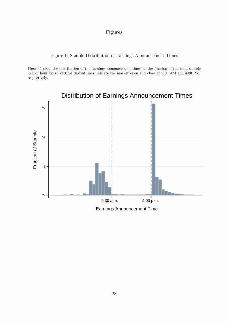
Figure 1 presents the intra-day distribution of the timing of earnings announcements

as the fraction of our sample in half hour windows throughout the day. The figure shows

that the vast majority of earnings announcements occur in the PO period (the four and

a half hours prior to the market open at 9:30 AM) or the PC (the four hours after

the market close at 4:00 PM).1 In our sample we have dropped the small fraction of

announcements that occur outside of the PO and PC hours. In our empirical analyses

we use a binary variable, PO, that is equal to one if the earnings announcement occurs

in the pre-open, and zero if the announcement occurs in the post-close. We also use a1The distribution of announcement times for our sample is similar to that reported by Michaely et al.

(2016).

8

continuous variable to measure the distance between the nearest open or close of regular

trading hours and the earnings announcement time. DIST is calculated as the absolute

value of the amount of time, in hours, between the market close and the announcement

time for PC announcements, or the market open and the announcement time for PO

announcements. For example, announcements at 4:30 PM and 9:00 AM would both

receive a DIST value of 0.5.

3.2. Variable Construction

Various estimates of volatility have been used extensively as proxies for information

around events (e.g., Bushee et al., 2011; Kirk and Markov, 2016; Matsumoto et al.,

2011). The basic intuition is straight forward. Consider an investor who applies Bayes

rule when setting equity prices. Such an investor makes revisions in beliefs about equity

prices as news about future cash flows and discount rates arrives. Value-relevant news

causes revisions in beliefs, which leads to revisions in stock prices. Estimated volatility

represents a measure of variation in the belief revisions through time. If an earnings

announcement is uninformative, all else equal, investors do not revise their beliefs and

volatility is flat. If an event has information, prices move and volatility increases.

Consistent with this, Patell and Wolfson (1979, 1981) examine the behavior of option-

implied as well as realized stock return volatility around earnings announcements. They

find that implied volatility increases before earnings announcements, in anticipation that

earnings news will carry value-relevant information that will increase stock price variabil-

ity. Patell and Wolfson (1981) use ex post realized volatility as a proxy for information

and indeed find that volatility increases on average following an earnings announcement.

Our empirical tests of the information in the timing of earnings are similarly motivated:

if announcing in the PO is associated with less attention to the announcement and there-

fore a delayed reaction to the announcement, then it is expected that volatility will be

higher in the days after the announcement for PO versus PC announcements. Like-

wise, if announcing farther from regular trading hours is associated with inattention, we

9

would expect the distance from regular trading hours to the announcment to be related

to volatility.

Our main empirical tests rely on volatility that is estimated using intraday trading

and quote data from TAQ. We calculate volatility from high frequency TAQ data for

two reasons: 1) volatility estimated from intraday data is considered a superior measure

of realized volatility than are estimates based on lower frequency data, such as daily or

weekly returns (Bollerslev et al., 2009); 2) we are interested in volatility estimated over

small windows around earnings events. TAQ data allows us to calculate volatility at high

frequency, this is not possible with daily data provided by CRSP.

We calculate volatility as follows. For each firm we collect volume-weighted average

prices (VWAPs) every minute from the TAQ execution files. We then construct volatility

over daily regular trading hours by summing the squared one-minute log-returns and then

taking the square root of the sum.2 We also calculate abnormal volatility to control for

common trends and persistence in firm-level volatility. We calculate abnormal volatility

(ABV OL) as the ratio of current volatility to the average historical volatility over the

same trading interval on the same trading day for the prior five weeks, excluding the

week before the earnings announcement, minus 1 and multiplied by 100. This allows

us to control for historical firm-level volatility behavior at identical trading times on

non-earnings announcement days.3

In addition to volatility, we measure abnormal volume, abnormal returns, and abnor-

mal bid-ask spreads around the earnings announcement. Abnormal volume (ABV OLUME)

is the total trading volume during the regular hours period as obtained from TAQ, nor-

malized using the same equation as ABV OL, i.e., dividing volume for firm i on day t

by the average volume on the same day of the week over four prior weeks, subtracting 1

and multiplying by 100. Abnormal spread (ABSPREAD) is the mean bid-ask spread,2We also calculate volatility for regular trading hours using mid-points instead of execution prices

to ensure that our results are not driven by microstructure noise. We find that our results are virtuallyidentical if we use mid points instead of execution prices.

3In untabulated robustness tests we find that varying the historical window we use to calculatehistorical volatility or using more sophisticated techniques, such as GARCH-based estimation, has verylittle impact on our results.

10

calculated per minute from TAQ, throughout the trading day normalized as above. Ab-

normal returns (ABRET ) are calculated daily using the Fama-French three factor model

and are multiplied by 100.

In Table 1 we present summary statistics for the full sample.4 Daily variables (ABV OL,

ABV OLUME, ABSPREAD, and ABRET ) are presented as the average of the three

day period from 0 to +2, where day 0 is the first full trading day immediately following

the release of earnings.5 For PO announcers, day 0 is the exact same calendar day that

earnings are announced, but for PC announcers, it is the following trading day. Mean

abnormal volatility is 61.49, indicating volatility following the earnings announcement

increases by approximately 61% compared to its historical volatility on the same days of

the week. Likewise, volume almost triples (165.59), and average abnormal returns are

slightly negative (-0.07), inconsistent with the prior literature that has documented, on

average, an earnings announcement premium (Barber et al., 2013).

SIZE is the natural log of the market capitalization of the firm (share price times

total shares outstanding). The book-to-market ratio of the firm (BM) is calculated as

the natural log of book value of equity divided by the market value of equity (share price

times the common shares outstanding). Return on equity (ROE) is natural log of one

plus the firm’s net income divided by its book value of equity. Unexpected earnings (or an

earnings surprise) (UE) is calculated as the earnings per share (EPS) from WSH, minus

the median analyst forecast from I/B/E/S, scaled by the stock price at the end of the

prior quarter, and multiplied by 100. If the firm has no analyst forecasts, the actual EPS

from the same quarter, prior year is used. The mean and median UE are 0.00. NUE is

an indicator equal to one if UE is negative, and zero otherwise. LEV is calculated as

total liabilities divided by total assets. IO is calculated quarterly as the percentage of

shares owned by institutions required to make 13-f filings. We measure the announcement

reporting lag (REPLAG) as the natural log of the number of days between the quarter4All variables are winsorized at the top and bottom 0.5%.5When calculating the three day ABV OL, the sum of squared log returns is taken over the three

day period before taking the square root for both the three day period of interest and the four referenceperiods.

11

end date and the earnings announcement date. The mean (median) analyst following

(ANALY STS) is 8.11 (6.00). Analyst dispersion (DISP ) is the standard deviation of

EPS forecasts that are used to calculate the consensus in I/B/E/S. We also calculate

the historical volatility (LAGV OL) as the log of the average intra-day volatility over the

prior six months and historical returns (LAGRET ) as the average returns over the prior

six months.

In our option-based tests we construct two different trading strategies with payoffs

that are directly linked to future stock return volatility: delta hedged returns (Bakshi

and Kapadia, 2003) and straddle returns (Coval and Shumway, 2001; Goyal and Saretto,

2009). Returns on delta hedge and straddle strategies are calculated as follows:

Delta Hedge Return: RDHt+1 = Ot+1 −∆tSt+1

Ot −∆tSt

− 1, (1)

Straddle Return: RSt+1 = Ct+1 + Pt+1

Ct + Pt

− 1. (2)

Here Ot represents the price of an option (a call or a put), Ct is the price of a call

option and Pt is the price of a put option. St is the price of the stock.

All options data are obtained from the IvyDB OptionMetrics database. We select all

options that have expirations at least three days following an earnings announcement.

From these, we keep only those options that are closest to at-the-money and have the

shortest expiration. For straddles, we construct put-call pairs, where the put and the call

have identical expiration and strike prices.

Table 1, Panel B presents the descriptive statistcs by distance to trading (DIST ).

We note that PO appears to be associated with distance to trading. Panel C of Table

1 presents the descriptive statistics for PO and PC announcements separately. We note

that there are significant differences in firm and earnings announcement characteristics

based on PO versus PC announcements. Because of this, we perform analyses with firm

fixed effects and propensity score matching.

12

Table 2 presents a correlation matrix of the variables used in the study. Consistent

with intuition, abnormal volatility is positively correlated with volume, bid-ask spreads,

and pre-open announcement (PO). It is negatively correlated with stock returns (consis-

tent with Ang et al., 2006, 2009) and book-to-market.

4. Empirical Tests

Our main empirical focus is on examining the difference in stock return volatility

for earnings announcements made farther from regular trading hours and for PO versus

PC earnings announcements. We initially test whether announcing farther from regular

trading hours and in the PO are significantly associated with abnormal volatility. We

also examine option-based trading strategies to determine if option traders price options

differently for PO and PC firms.

4.1. Abnormal Volatility

Panel A of Table 3 presents the mean difference in ABV OL, measured using daily

volatility from intraday prices, between PO and PC firm-quarters over days -5 to +5

around the announcement day, where day 0 is the first trading day following the an-

nouncement. Differences greater than zero indicate PO firms have higher abnormal

volatility than PC firms on average, and differences less than zero indicate PC firms

have higher volatility than PO firms. The differences support our first hypothesis related

to PO earnings announcements: following an earnings announcement, PO firms have

higher abnormal volatility than PC firms. Importantly, it is also clear that this is not a

one-day phenomenon. The abnormal volatility spread is close to zero three days before

the announcement, when it starts to turn negative and continues this trend until one

trading day prior to the earnings announcement, indicating that PO firms have lower

abnormal volatility going into an announcement. This trend reverses on the day of the

announcement, at which point the PO announcers’ volatility increases and remains above

the PC announcers’ volatility for approximately three days following the announcement.

13

Panel B of Table 3 presents the mean daily ABV OL across subsets of earnings an-

nouncements based on DIST , or the number of hours the earnings announcement is from

regular trading hours. The univariate statistics support our first hypothesis related to the

market reaction to earnings announcements released farther from regular trading hours.

Specifically, the table documents a decreasing trend in ABV OL as distance increases

in the days prior to the earnings announcement and an increasing trend in ABV OL as

distance increases in the days after the announcement. While we do not provide a hypoth-

esis regarding the lower volatility prior to the earnings announcement for announcements

farther from regular trading hours or in the PO, we control for the pre-announcement

volatility in our analyses.

Table 4 presents a formal test of Table 3. In Table 4 Panel A, we measure ABV OL as

the cumulative abnormal volatility over days +0 to +2, where day zero is the first trading

period following the earnings announcement. We regress ABV OL on PO, DIST , and

the interaction between PO and DIST and with year and industry fixed effects. We

include the interaction to determine if the relation between volatility, PO and DIST is

conditional upon PO and/or DIST .

It is possible the difference in volatility is simply a feature of the type of firm that

discloses farther from regular trading hours or in the PO versus the PC. So we control

for firm characteristics that could impact stock return volatility as well as proxies for

firms’ information environments. We control for size (SIZE), book-to-market (BM),

return on equity (ROE), leverage (LEV ), institutional ownership (IO), analyst follow-

ing (ANALY STS), analyst dispersion (DISP ), historical volatility (LAGV OL), and

historical returns (LAGRET ). Size, book-to-market, leverage, and return on equity are

all lagged one quarter, so the data are available prior to the announcement. The results

show that all but three (firm size, leverage, and analyst forecast dispersion) of the firm-

level control variables are significantly associated with abnormal volatility across all the

models.

It is also possible that our results may be driven by other earnings announcement char-

14

acteristics such as the abnormal volatility in the days prior to the earnings announcement,

the magnitude of the earnings surprise that is announced, the sign of the earnings sur-

prise, or the earnings reporting lag. To consider this possibility, we include controls for

abnormal volatility in the three days prior to the announcement (ABV OLP RE), unex-

pected earnings (UE), an indicator variable for negative unexpected earnings (NUE),

fourth quarter announcements (Q4), and the earnings reporting lag (REPLAG). The

results show that these earnings announcement controls are significantly associated with

abnormal volatility after the announcement.

Columns (1) through (3) include firm-level and earnings announcement character-

istic controls while columns (4) through (6) also include controls for contemporaneous

abnormal volume (ABV OLUME), abnormal returns (ABRET ), and abnormal bid-ask

spreads (ABSPREAD). In both specifications, the coefficient on PO and the coefficient

on DIST is positive and significant at the 1% level when included individually.

In Table 4 Panel B, we perform the same tests but include firm fixed effects in the

regression to ensure the results are not driven by a persistent firm-level characteristic not

captured by our control variables. Again, the results confirm the finding that abnormal

volatility for earnings announcements released farther from regular trading hours (DIST )

and PO earnings announcements are higher in the days after the announcement.

To ensure that our results are not driven by a single trading day, in untabulated

analyses we run daily regressions of abnormal volatility for each day from day 0 to day 5

where day 0 is the first trading day following the earnings announcement. We include all

of the control variables used in Table 4. The daily regressions are broadly consistent with

the univariate findings in Table 3. Post-announcement abnormal volatility is positively

associated with PO and DIST , but only on trading days, t = 0 through t = +3.

Despite including a number of firm and earnings announcement characteristics in our

regression analysis, there is a possibility that these characteristics could drive our results.

To ensure that this is not the case, we also perform a propensity score matching analysis.

Specifically, we estimate a model to explain whether a firm releases earnings PO versus

15

PC using all non-contemporaneous controls from Table 4 in the propensity score model.

Panel A of Table 5 reports the differences in the characteristics between the PO and

PC earnings announcements and Panel B reports the abnormal volatility results on the

propensity score matched sample.

The results in Panel A show that the matching achieves covariate balance on all the

variables except leverage and analyst coverage. These differences, though statistically

significant, are small in absolute magnitude. Overall, the matching process appears rea-

sonable and generates groups with similar characteristics. Table 5, Panel B shows that

the results are robust to propensity score matching. Specifically, abnormal volatility in

the days after the earnings announcement is significantly greater the farther the earnings

announcement is from regular trading hours (DIST ) and when the earnings announce-

ment is in the PO.

4.2. Robustness Tests

4.2.1. Placebo Tests

As a robustness test to ensure that our findings are not driven by firm characteris-

tics and differential trading behavior for firms that release earnings farther from regular

trading hours or in the PO, we perform two placebo tests. The first examines the re-

lation between abnormal volatility and PO and DIST during a non-announcement day

which is 21 days prior to the earnings announcement day. The results of this pseudo-

announcement test are reported in Panel A of Table 6. The second placebo test examines

the relation around a Federal Reserve meeting announcement and is reported in Panel

B of Table 6. We include the abnormal volatility in the following three days as the

dependent variable and the same explanatory variables as in previous analyses. If the

previous findings are not driven by firm characteristics, we expect no relation between

abnormal volatility and PO or DIST . Consistent with this, in both placebo tests, we

find insignificant relations between abnormal volatility and PO announcements and the

distance from regular trading hours.

16

4.2.2. Other Earnings Announcement Characteristics

We also examine whether the relations between abnormal volatility and PO and

DIST are incremental to other earnings announcement timing characteristics that have

been documented to be associated with investor inattention. Specifically, Hirshleifer

et al. (2009) find investor underreaction to earnings announcements released on days

with a greater number of earnings announcements from other firm and deHann et al.

(2015) document greater attention to earnings announcements that receive more advanced

warning. We therefore examine whether PO and DIST provide incremental information

content for abnormal volatility after controlling for earnings announcement frequency

(EAFREQ) and lead time (LEADTIME). To calculate EAFREQ, we measure the

number of contemporaneous earnings announcements on each day in Compustat and

define decile cutoffs for the population. EAFREQ is the decile number in which a

given earnings announcement day falls. The results of the analysis including this control

variable are reported in Panel A of Table 7. LEADTIME is defined as the logged lead

time (in days) between the date on which the firm schedules its earnings announcement

date and the EA date itself, and the results including this variable in the regression

are reported in Panel B of Table 7. We find that both PO and DIST continue to be

significantly positively associated with abnormal volatility after controlling for EAFREQ

and after controlling for LEADTIME.

We also perform robustness tests (untabulated) to include characteristics of the earn-

ings announcement that have been shown in prior research to be associated with the

market’s reaction to the announcement. Specifically, we reestimate the regressions in

Table 4 with an indicator variable for earnings announcements that are released on the

same day as the 10-K or 10-Q filing (Li and Ramesh, 2009), an indicator variable for

earnings announcements released prior to audit completion (Bronson et al., 2011), and

earnings announcements that are released with a management forecast included in the

announcement (Anilowski et al., 2007). We find that our main result, namely greater ab-

17

normal volatility in the three days after the announcement for earnings announcements

released farther from regular trading hours and in the PO, is robust to inclusion of these

variables.

4.2.3. Alternative Information Releases

One possible explanation for our results is that additional public information releases,

whether in the form of a conference call, annual or quarterly filing, analyst revision, or

news story, are delayed for PO announcements compared to PC announcements, which

might be a cause for a difference in volatility over the subsequent days. We perform

three tests (untabulated) to address this concern. First, we examine the distribution

of conference call times. For our sample, the vast majority of PO announcers hold the

call on the same day as the announcement and PC announcers split between the same

day they announce and the following trading day. Apart from this difference, we closely

inspect the empirical distribution of the time between the earnings announcement and the

conference call and find the distributions are similar. We also include the time between

announcement and conference call as an additional control in our regression analysis and

find that it has very little impact on our results. Second, we count the number of analyst

revisions on each day following the announcement as a proxy for additional news that

might generate trading and find our results are robust to the inclusion of this variable as

a control. Last, we collect from RavenPack news data and count the number of articles

published on each day following the announcement, again finding our results are robust

to this control. As a whole, it does not appear that public releases of other information

are driving our result.

4.2.4. Predictability Over Time

Our sample period includes the financial crisis, a rapid increase in equity prices fol-

lowing the crisis, and continued expansion of algorithmic trading. To ensure that our

results are not driven by a specific time period, we also performed empirical tests for

18

each year in our sample period. Our results indicate that the strong positive associations

between PO and DIST and abnormal volatility is not driven by a single year. In fact,

we find these significant relations with abnormal volatility for every year in our sample,

aside from 2011.

4.3. Option-Based Returns

Given the strong relations between abnormal volatility and announcing in the PO

versus the PC and the distance of the earnings announcement to regular trading hours,

we examine whether option markets anticipate the differential volatility response based on

PO and DIST . To do this, we construct two option-based trading strategies with payoffs

that are directly linked to future stock return volatility that are common for trading on

stock return volatility: delta hedged returns (Bakshi and Kapadia, 2003) and straddle

returns (Coval and Shumway, 2001; Goyal and Saretto, 2009). The goal of looking at

returns to these strategies is to determine if option traders impound the volatility spread

based on PO and DIST into option prices. If option traders anticipate this difference

then returns to these strategies should not be significantly related to PO and DIST .

We test this two ways. First, we conduct regressions using both option return strate-

gies as the dependent variable. Second, we form portfolios and determine if the returns to

these portfolios are sensitive to firm characteristics. Like our prior tests, our window of

interest is from the announcement day (t = 0) to two days following the announcement

(t = + 2), which represents three trading days in total.

Table 8 presents return regressions analysis results for both option strategies as well

as results for equity returns. For each strategy, we report the coefficient on PO and

DIST with the same controls as the previous analyses. Table 8 clearly shows that each

option strategy has strong positive associations with PO and DIST with economically

meaningful magnitudes. For example, the average daily return for a PO earnings an-

nouncement is approximately 0.29% higher for the delta hedge and 2.27% higher for the

straddle. The table also indicates that average stock returns are neither economically nor

19

statistically associated with PO and DIST .

To ensure that our regression-based results are not being driven by idiosyncratic noise

or the linear structure that is imposed by these tests, we also form portfolios. By forming

portfolios, we are able to reduce the potential impact from idiosyncratic noise through

the power of diversification and examine how returns to these portfolios vary with certain

firm characteristics. Table 9 presents portfolio returns of a long position in PO firms and

short position in PC firms, sorted on firm characteristics. Panel A shows the returns on

equity and each option-based strategy sorted on firm size (SIZE). Panel B shows the

same returns but sorts on historical volatility (LAGV OL). Panel C sorts on historical

bid-ask spread (LAGSPREAD). The results tell a similar story as the regression results

presented in Table 8. Returns on each of the option-based strategies are significant and

are not sensitive to firm characteristics, but equity returns are unrelated to announcing

in the PO or PC.

4.4. Market Return Reaction to Earnings Announcements

To provide additional insight into whether there is a delayed investor reaction to

earnings announcements released farther from regular trading hours or in the PO, we

examine the association between abnormal stock returns and the earnings surprise on the

day of the announcement and the intraperiod timeliness (IPT) of the reaction to earnings

news in the five days after the announcement. Panel A of Table 10 reports the results of

the announcement date returns, and Panel B reports the results of the IPT tests.

The dependent variable in the market reaction test (Panel A) is the size adjusted

abnormal returns on the day of the earnings announcement.6 We include the same ex-

planatory variables as in the previous analyses. Given that prior research finds a lower

market response to losses (Hayn, 1995), we include an interaction term, UE ∗ LOSS,

in the regression reported in the first set of columns. Prior research also documents a

lower market response to bad earnings news (Kothari, 2001), and as such we include an6We measure returns from the market close immediately prior to which earnings are announced to

the market close immediately after which earnings are announced.

20

interaction term, UE ∗NUE, in the second set of columns. To test for a muted reaction

to announcements released in the PO, we include an interaction term for PO and UE

(PO∗UE). To test for a muted reaction to earnings announcements released farther from

regular trading hours, we include an interaction term for DIST and UE (DIST ∗ UE).

Consistent with a muted reaction to the earnings announcement, we find a significant

negative coefficient on PO ∗ UE as well asDIST ∗ UE.7

In Panel B of Table 10, we report the results of the IPT test. The IPT captures the

speed with which information is incorporated into price after controlling for the price

response to the information (Twedt, 2016; Butler et al., 2007). The dependent variable

is the daily proportion of size-adjusted abnormal returns realized up to and including

a given day, starting on day 0 (the day of the earnings announcement) and continuing

through day +5. For each day, we calculate the cumulative buy-and-hold return from

day 0 to that day, scaled by the cumulative abnormal return for the entire period. We

then estimate the area under this curve for each earnings announcement, where a larger

area indicates that the information is more quickly impounded into price.

We regress the IPT metric on PO and DIST to test whether the market reacts less

quickly to earnings announced in the PO and farther from regular trading hours.8 We

include the same control variables as in the previous analyses. Consistent with a delayed

reaction to earnings released farther from regular trading hours and in the PO, we find

significant negative coefficients on PO and DIST .

Figure 2 provides graphical representation of the findings in Table 10. Panel A plots

the IPT metric for the days around the earnings announcement based on the distance of

the earnings announcement to regular trading hours. Panel B plots the IPT metric for

PO and PC firms. The figures show that the graphical depiction of the IPT metric is

consistent with the findings in Panel B of Table 10.7In Table 10, the contemporaneous controls do not include ABRET , as returns are the dependent

variable.8In this test, we truncate the sample at the top and bottom 1 percent of IPT value, as these

observations are primarily firms with net six-day abnormal returns extremely close to zero. In thesecases, the IPT measure is greatly inflated or deflated, as the total abnormal returns are the denominatorin the measure.

21

Overall, the findings of a muted reaction on the day of the announcement and a

delayed reaction in the five days after the announcement for earnings released farther

from regular trading hours and in the PO provides additional support for the notion that

investors are less attentive to these earnings announcements.

5. Conclusion

This paper documents that earnings announcements released farther from regular

trading hours and in the pre-open (before the opening bell) have higher abnormal volatil-

ity following the announcement relative to firms that announce closer to regular trading

hours and in the post-close (after the bell). This volatility difference persists for at least

three trading days following an earnings announcement and is highly predictable. It

cannot be explained by common determinants of volatility such as firm size, profitabil-

ity, volume, earnings surprises, stock returns, and historical volatility, and is not driven

by strategic announcement timing. Option trading strategies based on pre-open versus

post-close announcements and distance from regular trading hours yield economically

large returns, whereas trading strategies using equities yield economically insignificant

returns. We also find a muted market reaction to unexpected earnings on the day of the

announcement and slower incorporation of earnings news into prices over the five days

after the announcement for earnings released farther from regular trading hours and in

the PO. Collectively our results suggest that equity investors pay less attention and delay

the processing of earnings information when earnings are announced farther from regular

trading hours and in the pre-open. In addition, our results suggest that option traders

are unable to fully unravel this predictable phenomenon.

Our paper conjectures that investors process information differently for firms that

announce similar information farther from regular trading hours and in the morning

(the pre-open) versus the evening (the post-close); however, we cannot fully explain why

this happens. Research that can provide a more precise mechanism that can help us to

understand our robust empirical results represents a fruitful area of future work.

22

References

Ang, A., R. J. Hodrick, Y. Xing, and X. Zhang (2006). The cross-section of volatility

and expected returns. Journal of Finance 61 (1), 259–299.

Ang, A., R. J. Hodrick, Y. Xing, and X. Zhang (2009). High idiosyncratic volatility

and low returns: International and further U.S. evidence. Journal of Financial Eco-

nomics 91 (1), 1–23.

Anilowski, C., M. Feng, and D. J. Skinner (2007). Does earnings guidance affect market

returns? the nature and information content of aggregate earnings guidance. Journal

of Accounting and Economics 44 (1), 36–63.

Bagnoli, M., W. Kross, and S. G. Watts (2002). The information in management’s

expected earnings report date: A day late, a penny short. Journal of Accounting

Research 40 (5), 1275–1296.

Bakshi, G. and N. Kapadia (2003). Delta-hedged gains and the negative market volatility

risk premium. Review of Financial Studies 16 (2), 527–566.

Barber, B. M., E. T. De George, R. Lehavy, and B. Trueman (2013). The earnings

announcement premium around the globe. Journal of Financial Economics 108 (1),

118–138.

Barclay, M. J. and T. Hendershott (2003). Price discovery and trading after hours. Review

of Financial Studies 16 (4), 1041–1073.

Barclay, M. J. and T. Hendershott (2004). Liquidity externalities and adverse selection:

Evidence from trading after hours. The Journal of Finance 59 (2), 681–710.

Bollerslev, T., G. Tauchen, and H. Zhou (2009). Expected stock returns and variance

risk premia. Review of Financial studies 22 (11), 4463–4492.

23

Bradley, D., J. Clarke, S. Lee, and C. Ornthanalai (2014). Are analysts’ recommendations

informative? intraday evidence on the impact of time stamp delays. The Journal of

Finance 69 (2), 645–673.

Bronson, S. N., C. E. Hogan, M. F. Johnson, and K. Ramesh (2011). The unintended

consequences of pcaob auditing standard nos. 2 and 3 on the reliability of preliminary

earnings releases. Journal of Accounting and Economics 51 (1), 95–114.

Bushee, B. J., M. J. Jung, and G. S. Miller (2011). Conference presentations and the

disclosure milieu. Journal of Accounting Research 49 (5), 1163–1192.

Butler, M., A. Kraft, and I. S. Weiss (2007). The effect of reporting frequency on the

timeliness of earnings: The cases of voluntary and mandatory interim reports. Journal

of Accounting and Economics 43 (2), 181–217.

Carr, P. and L. Wu (2009). Variance risk premiums. Review of Financial Studies 22 (3),

1311–1341.

Coval, J. and T. Shumway (2001). Expected option returns. Journal of Finance 56 (3),

983–1009.

deHann, E., T. Shevlin, and J. Thornock (2015). Market (in) attention and the strategic

scheduling and timing of earnings announcements. Journal of Accounting and Eco-

nomics 60 (1), 36–55.

DellaVigna, S. and J. M. Pollet (2009). Investor inattention and Friday earnings an-

nouncements. The Journal of Finance 64 (2), 709–749.

Drake, M. S., K. H. Gee, and J. R. Thornock (2015). March market madness: The

impact of value-irrelevant events on the market pricing of earnings news. Contemporary

Accounting Research.

Drechsler, I. and A. Yaron (2011). What’s vol got to do with it. Review of Financial

Studies 24 (1), 1–45.

24

Engle, R. F. and V. K. Ng (1993). Measuring and testing the impact of news on volatility.

The Journal of Finance 48 (5), 1749–1778.

Gennotte, G. and B. Trueman (1996). The strategic timing of corporate disclosures.

Review of Financial Studies 9 (2), 665–690.

Goyal, A. and A. Saretto (2009). Cross-section of option returns and volatility. Journal

of Financial Economics 94 (2), 310–326.

Hayn, C. (1995). The information content of losses. Journal of accounting and eco-

nomics 20 (2), 125–153.

Hirshleifer, D., S. S. Lim, and S. H. Teoh (2009). Driven to distraction: Extraneous

events and underreaction to earnings news. The Journal of Finance 64 (5), 2289–2325.

Hirshleifer, D. and S. H. Teoh (2003). Limited attention, information disclosure, and

financial reporting. Journal of accounting and economics 36 (1), 337–386.

Hong, H. and J. C. Stein (1999). A unified theory of underreaction, momentum trading,

and overreaction in asset markets. The Journal of Finance 54 (6), 2143–2184.

Jiang, C. X., T. Likitapiwat, and T. H. McInish (2012). Information content of earn-

ings announcements: Evidence from after-hours trading. Journal of Financial and

Quantitative Analysis 47 (06), 1303–1330.

Kirk, M. and S. Markov (2016). Come on over: Analyst/investor days as a disclosure

medium. The Accounting Review 91 (6), 1725–1750.

Kothari, S. (2001). Capital markets research in accounting. Journal of accounting and

economics 31 (1), 105–231.

Li, E. X. and K. Ramesh (2009). Market reaction surrounding the filing of periodic sec

reports. The Accounting Review 84 (4), 1171–1208.

25

Li, J. (2016). Slow price adjustment to public news in after-hours trading. The Journal

of Trading 11 (3), 16–31.

Matsumoto, D., M. Pronk, and E. Roelofsen (2011). What makes conference calls useful?

the information content of managers’ presentations and analysts’ discussion sessions.

The Accounting Review 86 (4), 1383–1414.

Michaely, R., A. Rubin, and A. Vedrashko (2014). Corporate governance and the timing

of earnings announcements. Review of Finance 18 (6), 2003–2044.

Michaely, R., A. Rubin, and A. Vedrashko (2016). Further evidence on the strategic

timing of earnings news: Joint analysis of weekdays and times of day. Journal of

Accounting and Economics 62 (1), 24–45.

Pastor, L. and P. Veronesi (2009). Learning in financial markets. Annual Review of

Financial Economics 1 (1), 361–381.

Patell, J. M. and M. A. Wolfson (1979). Anticipated information releases reflected in call

option prices. Journal of Accounting and Economics 1 (2), 117–140.

Patell, J. M. and M. A. Wolfson (1981). The ex ante and ex post price effects of quarterly

earnings announcements reflected in option and stock prices. Journal of Accounting

Research, 434–458.

Patell, J. M. and M. A. Wolfson (1982). Good news, bad news, and the intraday timing

of corporate disclosures. The Accounting Review, 509–527.

Patell, J. M. and M. A. Wolfson (1984). The intraday speed of adjustment of stock prices

to earnings and dividend announcements. Journal of Financial Economics 13 (2), 223–

252.

Ross, S. A. (1989). Information and volatility: The no-arbitrage martingale approach to

timing and resolution irrelevancy. The Journal of Finance 44 (1), 1–17.

26

So, E. C. and J. Weber (2015). Time will tell: Information in the timing of scheduled

earnings news. Working paper .

Twedt, B. (2016). Spreading the word: Price discovery and newswire dissemination of

management earnings guidance. The Accounting Review 91 (1), 317–346.

27

Figures

Figure 1: Sample Distribution of Earnings Announcement Times

Figure 1 plots the distribution of the earnings announcement times as the fraction of the total samplein half hour bins. Vertical dashed lines indicate the market open and close at 9:30 AM and 4:00 PM,respectively.

0.1

.2.3

Fra

ctio

n of

Sam

ple

9:30 a.m. 4:00 p.m.

Earnings Announcement Time

Distribution of Earnings Announcement Times

28

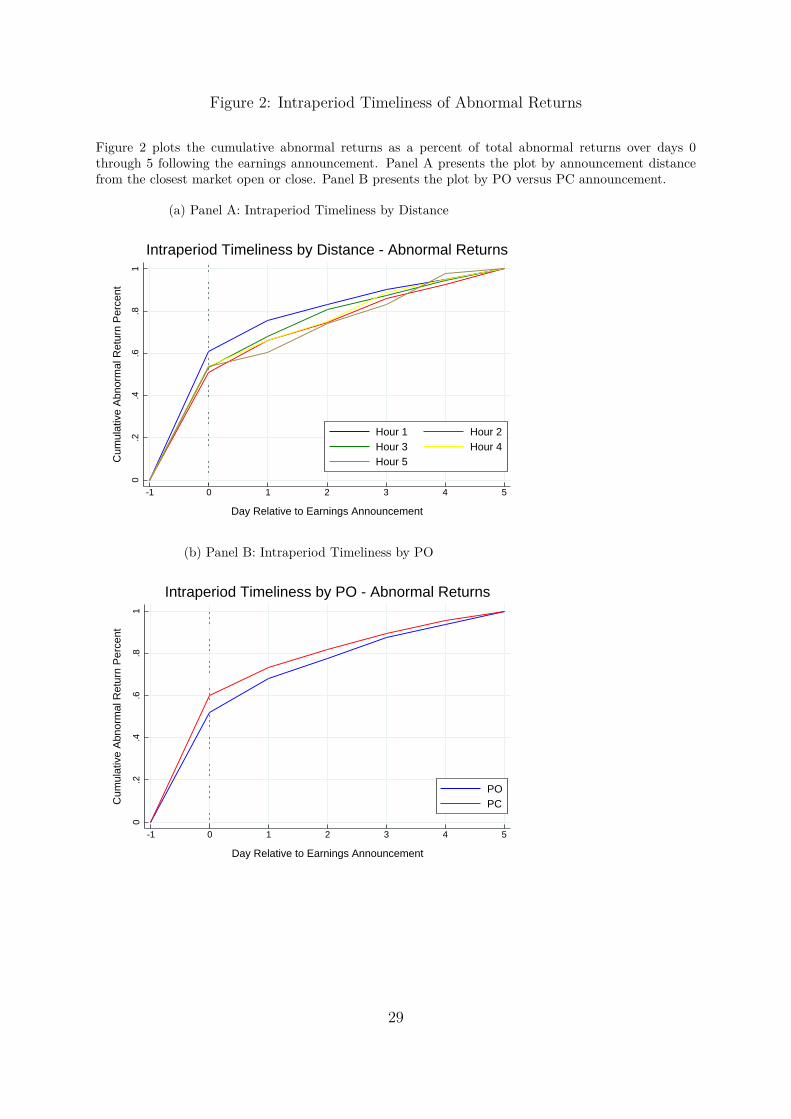
Figure 2: Intraperiod Timeliness of Abnormal Returns

Figure 2 plots the cumulative abnormal returns as a percent of total abnormal returns over days 0through 5 following the earnings announcement. Panel A presents the plot by announcement distancefrom the closest market open or close. Panel B presents the plot by PO versus PC announcement.

(a) Panel A: Intraperiod Timeliness by Distance

0.2

.4.6

.81

Cum

ulat

ive

Abn

orm

al R

etur

n P

erce

nt

-1 0 1 2 3 4 5

Day Relative to Earnings Announcement

Hour 1 Hour 2Hour 3 Hour 4Hour 5

Intraperiod Timeliness by Distance - Abnormal Returns

(b) Panel B: Intraperiod Timeliness by PO

0.2

.4.6

.81

Cum

ulat

ive

Abn

orm

al R

etur

n P

erce

nt

-1 0 1 2 3 4 5

Day Relative to Earnings Announcement

POPC

Intraperiod Timeliness by PO - Abnormal Returns

29

Tables

Table 1: Panel A, Summary Statistics

Table 1 presents summary statistics for key variables used in our study. Panel A presents the summarystatistics for the full sample. Panel B presents the mean values by announcement time distance fromthe nearest open or close (DIST ). Panel C presents the univariate differences between PO and PCannouncements. PO is an indicator equal to 1 if the firm announces in the pre-open period and 0if the firm announces in the post-close. DIST is the amount of time, in hours, between the earningsannouncement time and the nearest open or close of regular trading hours. ABV OL represents abnormalvolatility over the three day period from day 0 to +2, where day 0 is the first trading day after earningsare announced. ABV OLUME is abnormal volume from day 0 to +2. ABRET is the cumulativeabnormal return over day 0 to +2, calculated using the Fama-French three factor model, times 100.ABSPREAD is the average abnormal spread measured from day 0 to +2. SIZE is the natural log ofthe firm’s market value of equity (share price times the common shares outstanding). BM is the naturallog of the book value of equity divided by the market value of equity. ROE is the natural log of one plusnet income divided by the book value of equity. UE is the unexpected earnings of the firm, calculatedas the realized earnings per share less the consensus median estimate, scaled by the share price. LEVis the leverage of the firm, calculated as total liabilities divided by total assets. IO is the percentage ofthe firm’s shares owned by institutions required to make 13-f filings. REPLAG is the natural log of thenumber of days between the fiscal quarter end date and the earnings announcement date. ANALY STSis the number of analysts following the firm, measured as the number who contribute to the consensusEPS estimate prior to the earnings announcement. DISP is the standard deviation of the analyst EPSforecasts that make up the consensus forecast. LAGV OL is the mean daily volatility from -183 to -7days prior to the earnings announcement. LAGRET is the sum of the daily log returns over the period-183 to -7 days prior to the earnings announcement..

N Mean StDev P25 P50 P75

PO 80,630 0.47 0.50 0.00 0.00 1.00DIST 80,630 1.26 1.17 0.00 1.00 2.00ABV OL 80,630 61.49 71.50 16.71 45.23 86.02ABV OLUME 80,630 165.59 246.50 18.25 95.01 221.93ABRET 80,630 -0.07 7.27 -4.13 -0.18 3.89ABSPREAD 80,630 -1.04 25.20 -15.53 -1.68 10.03SIZE 80,630 7.10 1.60 5.92 6.95 8.09BM 80,630 -1.11 0.99 -1.65 -0.97 -0.42ROE 80,630 0.02 0.08 0.01 0.02 0.04UE 80,630 0.00 0.02 0.00 0.00 0.00NUE 80,630 0.34 0.47 0.00 0.00 1.00LEV 80,630 0.50 0.24 0.32 0.50 0.68IO 80,630 0.67 0.30 0.49 0.73 0.88REPLAG 80,630 3.45 0.33 3.22 3.47 3.64ANALY STS 80,630 8.11 6.80 3.00 6.00 11.00DISP 80,630 0.05 0.06 0.01 0.03 0.05LAGV OL 80,630 0.28 0.84 -0.29 0.27 0.81LAGRET 80,630 0.00 0.30 -0.14 0.02 0.16

30

Table 1: Panel B, Summary Statistics by Distance to Trading

Hours from Trading (→)0-1 1-2 2-3 3-4 4-5+

N 37,009 18,315 17,085 7,259 8,66PO 0.11 0.66 0.87 0.86 1.00DIST 0.21 1.36 2.34 3.34 4.62ABV OL 59.69 60.75 65.19 64.13 58.74ABV OLUME 195.21 137.67 144.26 137.81 148.71ABRET -0.08 -0.08 -0.04 -0.04 0.12ABSPREAD -2.61 0.46 0.19 0.27 -0.94SIZE 6.91 7.07 7.41 7.42 7.39BM -1.17 -0.95 -1.20 -1.08 -0.91ROE 0.01 0.02 0.02 0.02 0.02UE 0.00 0.00 0.00 0.00 0.00NUE 0.00 0.00 0.00 0.00 0.00LEV 0.47 0.54 0.52 0.54 0.48IO 0.66 0.65 0.69 0.68 0.63REPLAG 3.45 3.46 3.45 3.46 3.51ANALY STS 8.33 6.98 8.73 8.40 8.39DISP 0.04 0.05 0.05 0.06 0.05LAGV OL 0.22 0.30 0.32 0.38 0.37LAGRET 0.01 -0.02 -0.01 -0.01 -0.06

31

Table 1: Panel C, Summary Statistics by PO and PC

PO PCN Mean N Mean Diff t-stat

DIST 37,813 2.06 42,816 0.54 1.52 242.57ABV OL 37,813 64.69 42,816 60.16 4.53 8.53ABV OLUME 37,813 136.53 42,816 197.31 -60.78 -34.43ABRET 37,813 -0.08 42,816 -0.18 0.10 1.64ABSPREAD 37,813 0.65 42,816 -2.54 3.19 17.95SIZE 37,813 7.35 42,816 6.89 0.46 40.82BM 37,813 -1.12 42,816 -1.11 -0.01 -1.45ROE 37,813 0.02 42,816 0.01 0.01 10.86UE 37,813 0.00 42,816 0.00 0.00 -8.52NUE 37,813 0.36 42,816 0.32 0.04 11.64LEV 37,813 0.53 42,816 0.48 0.04 25.97IO 37,813 0.67 42,816 0.66 0.01 3.35REPLAG 37,813 3.44 42,816 3.46 -0.02 -6.41ANALY STS 37,813 8.29 42,816 7.96 0.33 6.76DISP 37,813 0.05 42,816 0.04 0.01 14.66LAGV OL 37,813 0.33 42,816 0.23 0.11 17.60LAGRET 37,813 -0.01 42,816 0.00 -0.01 -5.54

32

Tabl

e2:

Cor

rela

tion

Mat

rix

Tabl

e2

repo

rtst

heco

rrel

atio

nm

atrix

ofke

yva

riabl

esus

edin

the

anal

ysis

and

othe

rcom

mon

firm

-leve

lcha

ract

erist

ics.

See

Tabl

e1

forv

aria

ble

defin

ition

s.*

deno

tes

stat

istic

alsig

nific

ant

atth

e10

%le

vel.

(1)

(2)

(3)

(4)

(5)

(6)

(7)

(8)

(9)

(10)

(11)

(12)

(13)

(14)

(15)

(16)

(17)

(1)

PO

1.00

(2)

DIS

T0.

73*

1.00

(3)

AB

VO

L0.

03*

0.04

*1.

00(4

)A

BV

OL

UM

E-0

.17*

-0.1

4*0.

25*

1.00

(5)

AB

RE

T-0

.00

0.00

-0.0

3*-0

.05*

1.00

(6)

AB

SP

RE

AD

0.10

*0.

08*

0.26

*-0

.14*

0.21

*1.

00(7

)S

IZ

E0.

17*

0.11

*-0

.01*

-0.1

5*-0

.01*

0.10

*1.

00(8

)B

M0.

03*

0.05

*-0

.08*

-0.0

7*0.

000.

00-0

.20*

1.00

(9)

RO

E0.

04*

0.04

*0.

05*

0.03

*0.

07*

0.04

*0.

23*

-0.0

9*1.

00(1

0)U

E-0

.03*

-0.0

3*0.

000.

01*

0.13

*0.

05*

0.02

*-0

.05*

0.31

*1.

00(1

1)L

EV

0.05

*0.

04*

0.01

0.01

-0.2

3*-0

.09*

-0.0

7*0.

10*

-0.2

0*-0

.40*

1.00

(12)

IO

0.18

*0.

17*

-0.0

1-0

.14*

0.01

*0.

06*

0.28

*0.

02*

0.03

*-0

.05*

0.06

*1.

00(1

3)R

EP

LA

G0.

010.

03*

0.06

*0.

06*

0.04

*-0

.00

-0.0

3*-0

.02*

0.06

*-0

.01

-0.0

3*-0

.04*

1.00

(14)

AN

AL

YS

TS

-0.0

4*0.

000.

01*

0.04

*-0

.01

-0.0

4*-0

.34*

0.03

*-0

.14*

-0.0

3*0.

09*

-0.1

3*-0

.04*

1.00

(15)

DIS

P-0

.01

-0.0

2*-0

.04*

-0.0

6*0.

010.

05*

0.64

*-0

.12*

0.10

*0.

01*

-0.0

8*0.

09*

0.06

*-0

.29*

1.00

(16)

LA

GV

OL

0.08

*0.

09*

-0.0

5*-0

.08*

-0.0

2*0.

03*

0.08

*0.

22*

-0.1

1*-0

.14*

0.14

*0.

19*

0.02

*0.

06*

0.00

1.00

(17)

LA

GR

ET

0.04

*0.

04*

-0.0

5*-0

.03*

0.00

0.02

*0.

30*

-0.1

9*0.

15*

-0.0

2*-0

.02*

0.00

0.13

*-0

.07*

0.20

*0.

24*

1.00

33

Tabl

e3:

Pane

lA,A

bnor

mal

Vola

tility

byTr

adin

gD

ayfo

rPO

and

PCfir

ms

Tabl

e3

Pane

lApr

esen

tsth

eun

ivar

iate

daily

AB

VO

Lfr

omda

y-5

to+

5,w

here

day

0is

the

first

regu

lar

hour

str

adin

gda

yaf

ter

whi

chea

rnin

gsar

ean

noun

ced,

byP

O.

See

Tabl

e1

for

varia

ble

defin

ition

s.Pa

nelB

pres

ents

the

daily

AB

VO

Lby

the

anno

unce

men

ttim

edi

stan

cefr

omth

ene

ares

top

enor

clos

eof

regu

lar

trad

ing

hour

s.

POPC

NM

ean

NM

ean

Diff

t-st

at

t=−

537

,813

11.3

2742

,817

11.7

96-0

.469

-1.3

66t

=−

437

,813

12.3

9742

,817

12.6

94-0

.297

-0.8

49t

=−

337

,813

12.4

8442

,817

13.3

78-0

.894

-2.5

35t

=−

237

,813

14.0

4142

,817

16.4

11-2

.37

-6.5

76t

=−

137

,813

22.1

1342

,817

28.0

74-5

.961

-15.

334

t=

+0

37,8

1310

9.01

442

,817

106.

153

2.86

13.

709

t=

+1

37,8

1338

.538

42,8

1729

.598

8.94

19.6

t=

+2

37,8

1321

.494

42,8

1720

.477

1.01

72.

476

t=

+3

37,8

1317

.336

42,8

1715

.975

1.36

13.

567

t=

+4

37,8

1314

.997

42,8

1714

.571

0.42

61.

138

t=

+5

37,8

1314

.807

42,8

1714

.681

0.12

60.

328

34

Tabl

e3:

Pane

lB,A

bnor

mal

Vola

tility

byTr

adin

gD

ayan

dD

istan

ceto

Reg

ular

Trad

ing

Hou

rs

Hou

rsfro

mTr

adin

g(→

)0-

11-

22-

33-

44-

5+N

on-p

aram

eter

ictr

end

z-va

lue

N37

,009

18,3

1517

,085

7,25

986

6t

=−

511

.77

11.6

311

.51

10.7

710

.41

-2.4

0t

=−

412

.63

13.2

312

.11

11.6

011

.62

-2.4

8t

=−

313

.29

13.6

711

.88

11.9

213

.70

-2.6

3t

=−

216

.19

15.5

813

.88

13.4

614

.20

-6.9

7t

=−

128

.18

23.5

022

.53

22.2

119

.30

-15.

75t

=+

010

6.86

103.

1711

2.31

111.

2910

1.15

3.81

t=

+1

29.9

536

.24

37.9

936

.75

36.7

217

.46

t=

+2

20.3

121

.63

21.4

821

.31

20.4

03.

92t

=+

315

.86

17.5

617

.18

16.6

116

.06

3.87

t=

+4

14.1

815

.53

14.9

215

.31

16.3

93.

40t

=+

514

.49

14.9

314

.70

15.7

413

.44

1.75

35

Table 4: Panel A, Post-Announcment Abnormal Volatility Regressions

Table 4 presents the results of regressions of ABV OL on PO and DIST . Panel A presents the post-announcement abnormal volatility measured from day 0 to +2, where day zero is the first trading dayafter earnings are announced, without firm fixed effects. Panel B presents the same regressions with firmfixed effects. See Table 1 for variable definitions. . Q4 is an indicator equal to 1 if it is the firm’s fiscalfourth quarter, and 0 otherwise. Standard errors are clustered by earnings announcement date. *, **,and *** denote two-tailed statistical significance at the 10%, 5%, and 1% levels, respectively.

(1) (2) (3) (4) (5) (6)

P O 6.20*** 3.11*** 7.21*** 4.71***(6.95) (2.59) (9.00) (4.24)

DIST 2.30*** 0.34 2.63*** 0.79*(7.85) (0.79) (10.03) (1.95)

P O × DIST 1.26** 0.66(2.23) (1.23)

ABV OLUME 0.08*** 0.08*** 0.08***(26.46) (26.39) (26.48)

ABRET -0.82*** -0.82*** -0.82***(-15.96) (-15.96) (-15.97)

ABSP READ 0.86*** 0.86*** 0.86***(19.23) (19.35) (19.23)

ABV OLP RE 0.50*** 0.49*** 0.50*** 0.35*** 0.35*** 0.35***(20.47) (20.52) (20.48) (20.15) (20.21) (20.16)

UE -53.17*** -53.04*** -52.82*** -45.63*** -45.47*** -45.03***(-3.43) (-3.42) (-3.41) (-3.12) (-3.11) (-3.08)

NUE 4.85*** 4.89*** 4.87*** 3.84*** 3.91*** 3.84***(7.75) (7.84) (7.78) (6.69) (6.84) (6.69)

SIZE -0.33 -0.24 -0.37 0.84*** 0.94*** 0.79***(-1.30) (-0.95) (-1.47) (3.30) (3.70) (3.11)

BM -3.64*** -3.66*** -3.64*** -3.17*** -3.21*** -3.20***(-11.83) (-11.92) (-11.81) (-11.34) (-11.48) (-11.39)

ROE 26.30*** 26.27*** 26.36*** 21.24*** 21.27*** 21.20***(7.96) (7.97) (7.99) (7.10) (7.12) (7.09)

LEV 1.34 1.44 1.35 3.15*** 3.26*** 3.07***(1.03) (1.11) (1.04) (2.70) (2.78) (2.61)

IO 20.19*** 19.92*** 20.06*** 19.81*** 19.53*** 19.70***(19.10) (18.81) (18.97) (18.27) (18.05) (18.18)

REP LAG 8.21*** 7.92*** 8.09*** 8.38*** 8.04*** 8.27***(3.59) (3.46) (3.54) (4.23) (4.07) (4.17)

Q4 -5.03** -4.98** -5.00** -5.79*** -5.69*** -5.77***(-2.53) (-2.50) (-2.51) (-3.50) (-3.45) (-3.49)

ANALY ST S 0.18*** 0.18*** 0.18*** 0.10** 0.09** 0.10**(3.52) (3.46) (3.52) (2.02) (1.96) (2.13)

DISP 2.07 2.12 1.98 -2.31 -2.26 -2.38(0.48) (0.50) (0.47) (-0.59) (-0.58) (-0.61)

LAGV OL -2.58*** -2.61*** -2.56*** -3.10*** -3.14*** -3.10***(-6.11) (-6.18) (-6.08) (-7.94) (-8.04) (-7.94)

LAGRET 5.54*** 5.58*** 5.58*** -0.62 -0.57 -0.56(4.10) (4.14) (4.13) (-0.53) (-0.50) (-0.49)

# Observations 80,630 80,630 80,630 80,630 80,630 80,630R2 0.15 0.15 0.15 0.28 0.27 0.28Year and Industry FE Yes Yes Yes Yes Yes Yes

36

Table 4: Panel B, Post-Announcement Abnormal Volatility Regressions with Firm FixedEffects

(1) (2) (3) (4) (5) (6)

PO 5.98*** 5.50*** 6.52*** 6.84***(5.30) (3.09) (6.26) (4.09)

DIST 1.69*** 0.99* 1.61*** 0.94*(4.31) (1.75) (4.39) (1.78)

PO ×DIST -0.38 -0.75(-0.43) (-0.92)

ABV OLUME 0.08*** 0.08*** 0.08***(25.24) (25.21) (25.24)

ABRET -0.82*** -0.82*** -0.82***(-15.99) (-15.96) (-15.97)

ABSPREAD 0.89*** 0.89*** 0.89***(19.44) (19.47) (19.44)

ABV OLP RE 0.50*** 0.49*** 0.50*** 0.34*** 0.34*** 0.34***(19.95) (19.96) (19.96) (20.20) (20.21) (20.20)

UE 7.37 7.62 7.37 5.02 5.35 5.02(0.43) (0.45) (0.43) (0.30) (0.32) (0.30)

NUE 5.74*** 5.71*** 5.72*** 4.44*** 4.43*** 4.42***(8.99) (8.96) (8.96) (7.46) (7.44) (7.43)

SIZE 6.70*** 6.79*** 6.73*** 6.82*** 6.93*** 6.86***(5.15) (5.21) (5.17) (6.03) (6.11) (6.06)

BM -1.11 -1.12 -1.11 -1.72*** -1.74*** -1.73***(-1.58) (-1.59) (-1.59) (-2.61) (-2.62) (-2.62)

ROE -2.50 -2.42 -2.41 -2.52 -2.46 -2.46(-0.58) (-0.57) (-0.56) (-0.63) (-0.61) (-0.61)

LEV 13.88*** 13.83*** 13.82*** 5.92* 5.89* 5.84*(3.66) (3.64) (3.64) (1.68) (1.68) (1.66)

IO 5.65** 5.62** 5.69** 3.26 3.22 3.31(2.54) (2.53) (2.56) (1.61) (1.59) (1.63)

REPLAG 1.86 1.90 1.83 4.55** 4.61** 4.51**(0.77) (0.79) (0.75) (2.01) (2.03) (1.99)

Q4 -2.84 -2.89 -2.87 -4.33*** -4.36*** -4.35***(-1.51) (-1.53) (-1.52) (-2.65) (-2.67) (-2.66)

ANALY STS 0.56*** 0.55*** 0.56*** 0.37*** 0.36*** 0.37***(4.61) (4.54) (4.60) (3.23) (3.16) (3.24)

DISP 7.13 6.97 7.06 5.96 5.80 5.89(1.25) (1.22) (1.24) (1.12) (1.09) (1.10)

LAGV OL -6.00*** -6.02*** -6.02*** -4.75*** -4.77*** -4.77***(-7.26) (-7.27) (-7.27) (-6.91) (-6.94) (-6.93)

LAGRET 3.15* 3.18** 3.16* -2.94** -2.91** -2.93**(1.95) (1.97) (1.95) (-2.19) (-2.17) (-2.18)

# Observations 80,630 80,630 80,630 80,630 80,630 80,630R2 0.25 0.25 0.25 0.36 0.36 0.36Year and Firm FE Yes Yes Yes Yes Yes Yes

37

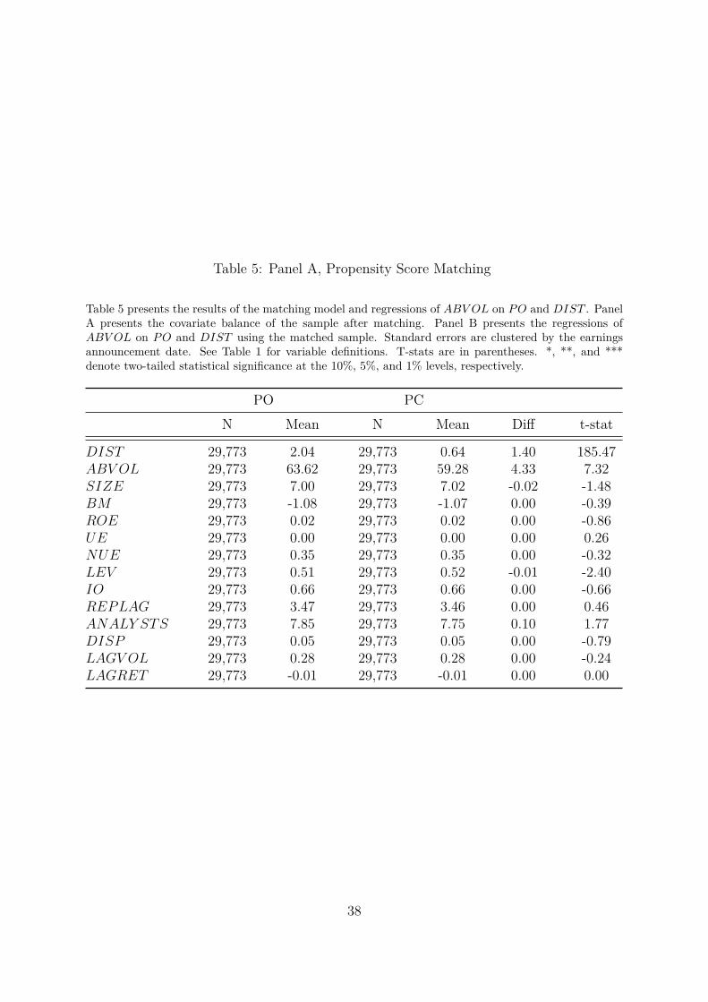
Table 5: Panel A, Propensity Score Matching

Table 5 presents the results of the matching model and regressions of ABV OL on PO and DIST . PanelA presents the covariate balance of the sample after matching. Panel B presents the regressions ofABV OL on PO and DIST using the matched sample. Standard errors are clustered by the earningsannouncement date. See Table 1 for variable definitions. T-stats are in parentheses. *, **, and ***denote two-tailed statistical significance at the 10%, 5%, and 1% levels, respectively.

PO PCN Mean N Mean Diff t-stat

DIST 29,773 2.04 29,773 0.64 1.40 185.47ABV OL 29,773 63.62 29,773 59.28 4.33 7.32SIZE 29,773 7.00 29,773 7.02 -0.02 -1.48BM 29,773 -1.08 29,773 -1.07 0.00 -0.39ROE 29,773 0.02 29,773 0.02 0.00 -0.86UE 29,773 0.00 29,773 0.00 0.00 0.26NUE 29,773 0.35 29,773 0.35 0.00 -0.32LEV 29,773 0.51 29,773 0.52 -0.01 -2.40IO 29,773 0.66 29,773 0.66 0.00 -0.66REPLAG 29,773 3.47 29,773 3.46 0.00 0.46ANALY STS 29,773 7.85 29,773 7.75 0.10 1.77DISP 29,773 0.05 29,773 0.05 0.00 -0.79LAGV OL 29,773 0.28 29,773 0.28 0.00 -0.24LAGRET 29,773 -0.01 29,773 -0.01 0.00 0.00

38

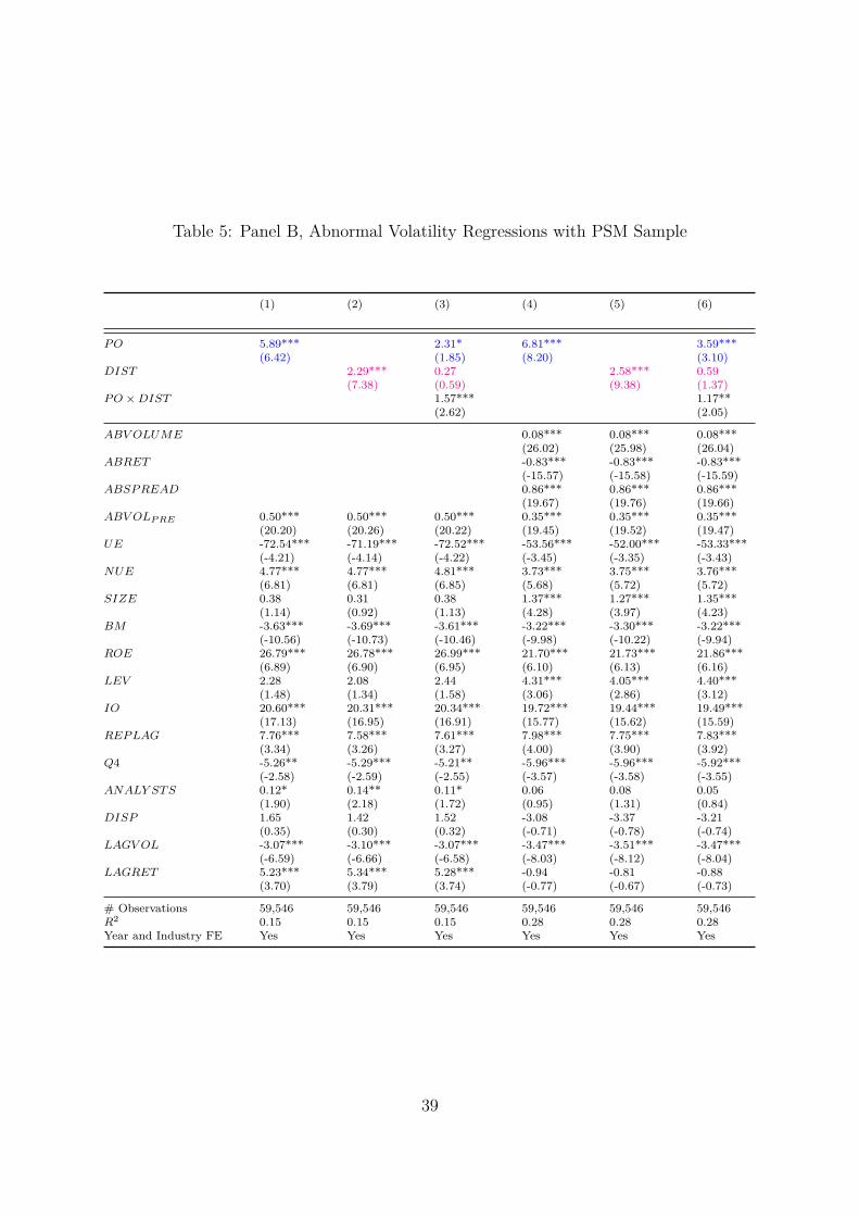
Table 5: Panel B, Abnormal Volatility Regressions with PSM Sample

(1) (2) (3) (4) (5) (6)

P O 5.89*** 2.31* 6.81*** 3.59***(6.42) (1.85) (8.20) (3.10)

DIST 2.29*** 0.27 2.58*** 0.59(7.38) (0.59) (9.38) (1.37)

P O × DIST 1.57*** 1.17**(2.62) (2.05)

ABV OLUME 0.08*** 0.08*** 0.08***(26.02) (25.98) (26.04)

ABRET -0.83*** -0.83*** -0.83***(-15.57) (-15.58) (-15.59)

ABSP READ 0.86*** 0.86*** 0.86***(19.67) (19.76) (19.66)

ABV OLP RE 0.50*** 0.50*** 0.50*** 0.35*** 0.35*** 0.35***(20.20) (20.26) (20.22) (19.45) (19.52) (19.47)

UE -72.54*** -71.19*** -72.52*** -53.56*** -52.00*** -53.33***(-4.21) (-4.14) (-4.22) (-3.45) (-3.35) (-3.43)

NUE 4.77*** 4.77*** 4.81*** 3.73*** 3.75*** 3.76***(6.81) (6.81) (6.85) (5.68) (5.72) (5.72)

SIZE 0.38 0.31 0.38 1.37*** 1.27*** 1.35***(1.14) (0.92) (1.13) (4.28) (3.97) (4.23)

BM -3.63*** -3.69*** -3.61*** -3.22*** -3.30*** -3.22***(-10.56) (-10.73) (-10.46) (-9.98) (-10.22) (-9.94)

ROE 26.79*** 26.78*** 26.99*** 21.70*** 21.73*** 21.86***(6.89) (6.90) (6.95) (6.10) (6.13) (6.16)

LEV 2.28 2.08 2.44 4.31*** 4.05*** 4.40***(1.48) (1.34) (1.58) (3.06) (2.86) (3.12)

IO 20.60*** 20.31*** 20.34*** 19.72*** 19.44*** 19.49***(17.13) (16.95) (16.91) (15.77) (15.62) (15.59)

REP LAG 7.76*** 7.58*** 7.61*** 7.98*** 7.75*** 7.83***(3.34) (3.26) (3.27) (4.00) (3.90) (3.92)

Q4 -5.26** -5.29*** -5.21** -5.96*** -5.96*** -5.92***(-2.58) (-2.59) (-2.55) (-3.57) (-3.58) (-3.55)

ANALY ST S 0.12* 0.14** 0.11* 0.06 0.08 0.05(1.90) (2.18) (1.72) (0.95) (1.31) (0.84)

DISP 1.65 1.42 1.52 -3.08 -3.37 -3.21(0.35) (0.30) (0.32) (-0.71) (-0.78) (-0.74)

LAGV OL -3.07*** -3.10*** -3.07*** -3.47*** -3.51*** -3.47***(-6.59) (-6.66) (-6.58) (-8.03) (-8.12) (-8.04)

LAGRET 5.23*** 5.34*** 5.28*** -0.94 -0.81 -0.88(3.70) (3.79) (3.74) (-0.77) (-0.67) (-0.73)

# Observations 59,546 59,546 59,546 59,546 59,546 59,546R2 0.15 0.15 0.15 0.28 0.28 0.28Year and Industry FE Yes Yes Yes Yes Yes Yes

39

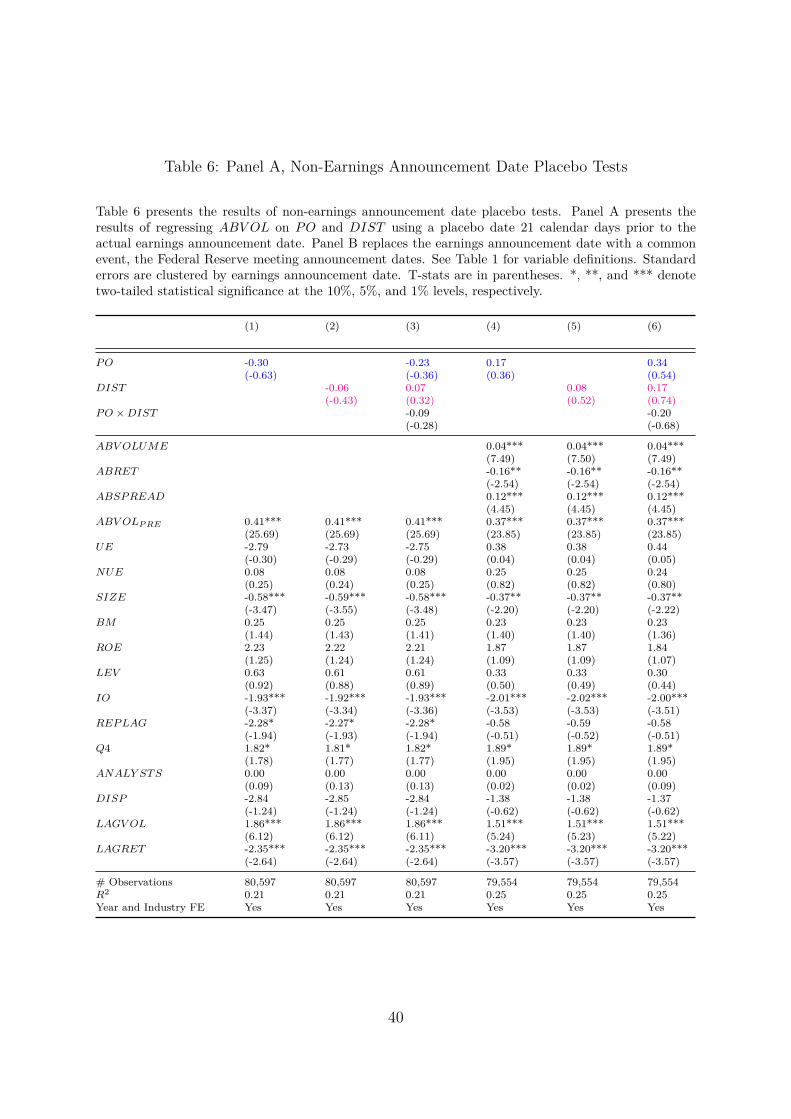
Table 6: Panel A, Non-Earnings Announcement Date Placebo Tests

Table 6 presents the results of non-earnings announcement date placebo tests. Panel A presents theresults of regressing ABV OL on PO and DIST using a placebo date 21 calendar days prior to theactual earnings announcement date. Panel B replaces the earnings announcement date with a commonevent, the Federal Reserve meeting announcement dates. See Table 1 for variable definitions. Standarderrors are clustered by earnings announcement date. T-stats are in parentheses. *, **, and *** denotetwo-tailed statistical significance at the 10%, 5%, and 1% levels, respectively.

(1) (2) (3) (4) (5) (6)

P O -0.30 -0.23 0.17 0.34(-0.63) (-0.36) (0.36) (0.54)

DIST -0.06 0.07 0.08 0.17(-0.43) (0.32) (0.52) (0.74)

P O × DIST -0.09 -0.20(-0.28) (-0.68)

ABV OLUME 0.04*** 0.04*** 0.04***(7.49) (7.50) (7.49)

ABRET -0.16** -0.16** -0.16**(-2.54) (-2.54) (-2.54)

ABSP READ 0.12*** 0.12*** 0.12***(4.45) (4.45) (4.45)

ABV OLP RE 0.41*** 0.41*** 0.41*** 0.37*** 0.37*** 0.37***(25.69) (25.69) (25.69) (23.85) (23.85) (23.85)

UE -2.79 -2.73 -2.75 0.38 0.38 0.44(-0.30) (-0.29) (-0.29) (0.04) (0.04) (0.05)

NUE 0.08 0.08 0.08 0.25 0.25 0.24(0.25) (0.24) (0.25) (0.82) (0.82) (0.80)

SIZE -0.58*** -0.59*** -0.58*** -0.37** -0.37** -0.37**(-3.47) (-3.55) (-3.48) (-2.20) (-2.20) (-2.22)

BM 0.25 0.25 0.25 0.23 0.23 0.23(1.44) (1.43) (1.41) (1.40) (1.40) (1.36)

ROE 2.23 2.22 2.21 1.87 1.87 1.84(1.25) (1.24) (1.24) (1.09) (1.09) (1.07)

LEV 0.63 0.61 0.61 0.33 0.33 0.30(0.92) (0.88) (0.89) (0.50) (0.49) (0.44)

IO -1.93*** -1.92*** -1.93*** -2.01*** -2.02*** -2.00***(-3.37) (-3.34) (-3.36) (-3.53) (-3.53) (-3.51)

REP LAG -2.28* -2.27* -2.28* -0.58 -0.59 -0.58(-1.94) (-1.93) (-1.94) (-0.51) (-0.52) (-0.51)

Q4 1.82* 1.81* 1.82* 1.89* 1.89* 1.89*(1.78) (1.77) (1.77) (1.95) (1.95) (1.95)

ANALY ST S 0.00 0.00 0.00 0.00 0.00 0.00(0.09) (0.13) (0.13) (0.02) (0.02) (0.09)

DISP -2.84 -2.85 -2.84 -1.38 -1.38 -1.37(-1.24) (-1.24) (-1.24) (-0.62) (-0.62) (-0.62)

LAGV OL 1.86*** 1.86*** 1.86*** 1.51*** 1.51*** 1.51***(6.12) (6.12) (6.11) (5.24) (5.23) (5.22)

LAGRET -2.35*** -2.35*** -2.35*** -3.20*** -3.20*** -3.20***(-2.64) (-2.64) (-2.64) (-3.57) (-3.57) (-3.57)

# Observations 80,597 80,597 80,597 79,554 79,554 79,554R2 0.21 0.21 0.21 0.25 0.25 0.25Year and Industry FE Yes Yes Yes Yes Yes Yes

40

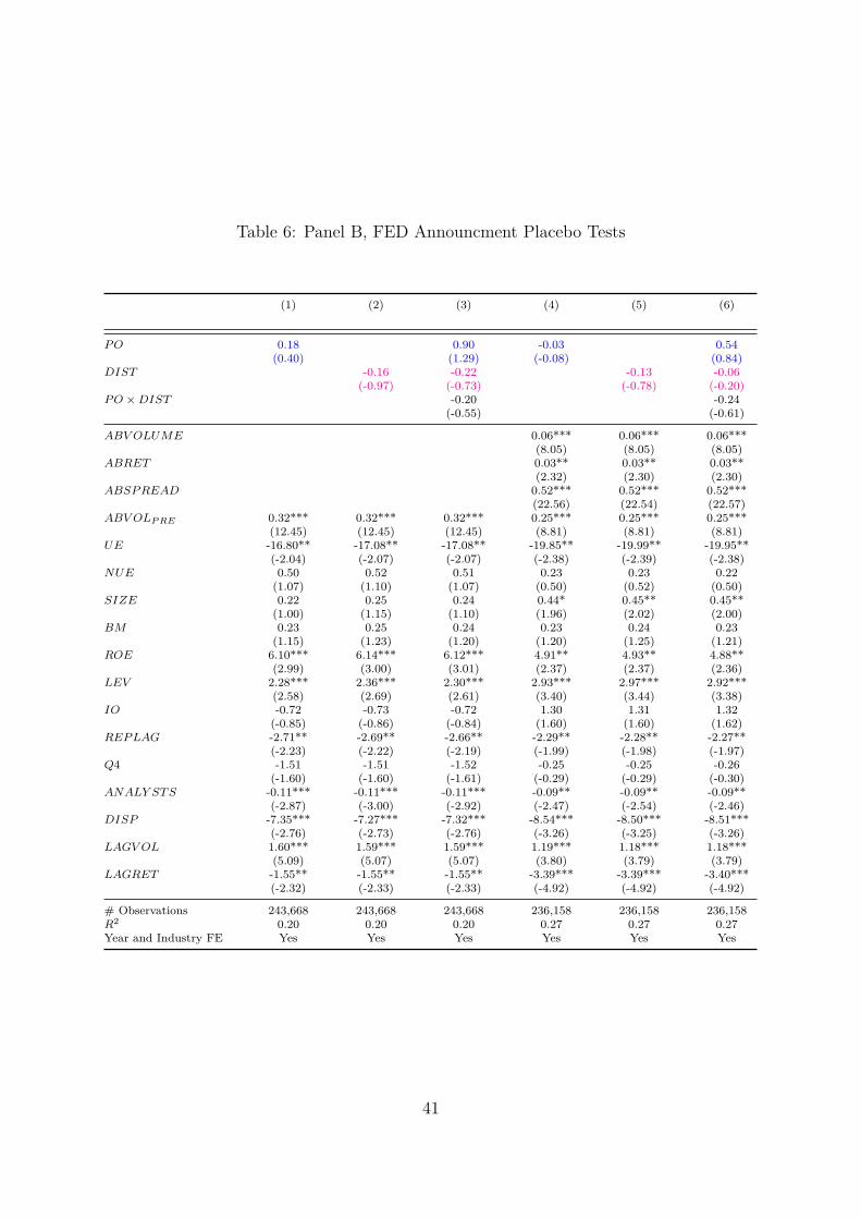
Table 6: Panel B, FED Announcment Placebo Tests

(1) (2) (3) (4) (5) (6)

P O 0.18 0.90 -0.03 0.54(0.40) (1.29) (-0.08) (0.84)

DIST -0.16 -0.22 -0.13 -0.06(-0.97) (-0.73) (-0.78) (-0.20)

P O × DIST -0.20 -0.24(-0.55) (-0.61)

ABV OLUME 0.06*** 0.06*** 0.06***(8.05) (8.05) (8.05)

ABRET 0.03** 0.03** 0.03**(2.32) (2.30) (2.30)

ABSP READ 0.52*** 0.52*** 0.52***(22.56) (22.54) (22.57)

ABV OLP RE 0.32*** 0.32*** 0.32*** 0.25*** 0.25*** 0.25***(12.45) (12.45) (12.45) (8.81) (8.81) (8.81)

UE -16.80** -17.08** -17.08** -19.85** -19.99** -19.95**(-2.04) (-2.07) (-2.07) (-2.38) (-2.39) (-2.38)

NUE 0.50 0.52 0.51 0.23 0.23 0.22(1.07) (1.10) (1.07) (0.50) (0.52) (0.50)

SIZE 0.22 0.25 0.24 0.44* 0.45** 0.45**(1.00) (1.15) (1.10) (1.96) (2.02) (2.00)

BM 0.23 0.25 0.24 0.23 0.24 0.23(1.15) (1.23) (1.20) (1.20) (1.25) (1.21)

ROE 6.10*** 6.14*** 6.12*** 4.91** 4.93** 4.88**(2.99) (3.00) (3.01) (2.37) (2.37) (2.36)

LEV 2.28*** 2.36*** 2.30*** 2.93*** 2.97*** 2.92***(2.58) (2.69) (2.61) (3.40) (3.44) (3.38)

IO -0.72 -0.73 -0.72 1.30 1.31 1.32(-0.85) (-0.86) (-0.84) (1.60) (1.60) (1.62)

REP LAG -2.71** -2.69** -2.66** -2.29** -2.28** -2.27**(-2.23) (-2.22) (-2.19) (-1.99) (-1.98) (-1.97)

Q4 -1.51 -1.51 -1.52 -0.25 -0.25 -0.26(-1.60) (-1.60) (-1.61) (-0.29) (-0.29) (-0.30)

ANALY ST S -0.11*** -0.11*** -0.11*** -0.09** -0.09** -0.09**(-2.87) (-3.00) (-2.92) (-2.47) (-2.54) (-2.46)

DISP -7.35*** -7.27*** -7.32*** -8.54*** -8.50*** -8.51***(-2.76) (-2.73) (-2.76) (-3.26) (-3.25) (-3.26)

LAGV OL 1.60*** 1.59*** 1.59*** 1.19*** 1.18*** 1.18***(5.09) (5.07) (5.07) (3.80) (3.79) (3.79)

LAGRET -1.55** -1.55** -1.55** -3.39*** -3.39*** -3.40***(-2.32) (-2.33) (-2.33) (-4.92) (-4.92) (-4.92)

# Observations 243,668 243,668 243,668 236,158 236,158 236,158R2 0.20 0.20 0.20 0.27 0.27 0.27Year and Industry FE Yes Yes Yes Yes Yes Yes

41

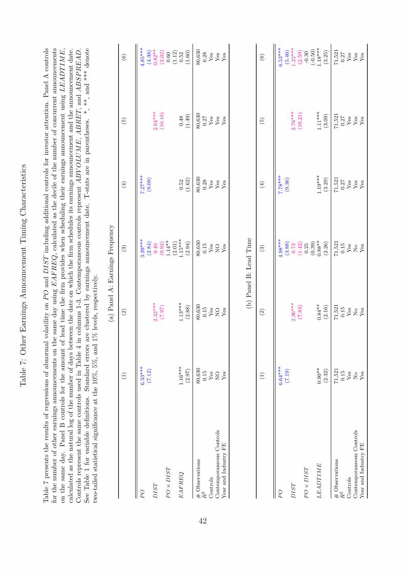
Tabl

e7:

Oth

erEa

rnin

gsA

nnou

ncem

ent

Tim

ing

Cha

ract

erist

ics

Tabl

e7

pres

ents

the

resu

ltsof

regr

essio

nsof

abno

rmal

vola

tility

onP

Oan

dD

IS

Tin

clud

ing

addi

tiona

lcon

trol

sfo

rin

vest

orat

tent

ion.

Pane

lAco

ntro

lsfo

rth

enu

mbe

rof

othe

rea

rnin

gsan

noun

cem

ents

onth

esa

me

day

usin

gE

AF

RE

Q,c

alcu

late

das

the

deci

leof

the

num

ber

ofco

ncur

rent

anno

unce

men

tson

the

sam

eda

y.Pa

nel

Bco

ntro

lsfo

rth

eam

ount

ofle

adtim

eth

efir

mpr

ovid

esw

hen

sche

dulin

gth

eir

earn

ings

anno

unce

men

tus

ing

LE

AD

TIM

E,

calc

ulat

edas

the

natu

rall

ogof

the

num

ber

ofda

ysbe

twee

nth

eda

teon

whi

chth

efir

msc

hedu

les

itsea

rnin

gsan

noun

cem

ent

and

the

anno

unce

men

tda

te.

Con

trol

sre

pres

ent

the

sam

eco

ntro

lsus

edin

Tabl

e4

inco

lum

ns1-

3.C

onte

mpo

rane

ous

cont

rols

repr

esen

tA

BV

OL

UM

E,A

BR

ET

,an

dA

BS

PR

EA

D.

See

Tabl

e1

for

varia

ble

defin

ition

s.St

anda

rder

rors

are

clus

tere

dby

earn

ings

anno

unce

men

tda

te.

T-s

tats

are

inpa

rent

hese

s.*,

**,

and

***

deno

tetw

o-ta

iled

stat

istic

alsig

nific

ance

atth

e10

%,5

%,a

nd1%

leve

ls,re

spec

tivel

y.

(a)

Pane

lA:E

arni

ngs

Freq

uenc

y

(1)

(2)

(3)

(4)

(5)

(6)

PO

6.33

***

3.39

***

7.27

***

4.85

***

(7.1

2)(2

.84)

(9.0

9)(4

.38)

DIS

T2.

33**

*0.

402.

64**

*0.

82**

(7.9

7)(0

.92)

(10.

10)

(2.0

2)P

O×

DIS

T1.

14**

0.60

(2.0

1)(1

.12)

EA

FR

EQ

1.16

***

1.13

***

1.15

***

0.52

0.48

0.52

(2.9

7)(2

.88)

(2.9

4)(1

.62)

(1.4

9)(1

.60)

#O

bser

vati

ons

80,6

3080

,630

80,6

3080

,630

80,6

3080

,630

R2

0.15

0.15

0.15

0.28

0.27

0.28

Con

trol

sY

esY

esY

esY

esY

esY

esC

onte

mpo

rane

ous

Con

trol

sN

ON

ON

OY

esY

esY

esY

ear

and

Indu

stry

FE

Yes

Yes

Yes

Yes

Yes

Yes

(b)

Pane

lB:L

ead

Tim

e

(1)

(2)

(3)

(4)

(5)

(6)

PO

6.64

***

4.98

***

7.78

***

6.53

***

(7.1

9)(3

.88)

(9.3

6)(5

.46)

DIS

T2.

36**

*0.

732.

76**

*1.

22**

*(7

.83)

(1.4

2)(1

0.21

)(2

.59)

PO

×D

IS

T0.

25-0

.30

(0.3

9)(-

0.50

)L

EA

DT

IM

E0.

90**

0.84

**0.

88**

1.19

***

1.11

***

1.18

***

(2.3

2)(2

.16)

(2.2

6)(3

.29)

(3.0

9)(3

.25)

#O

bser

vati

ons

71,5

2171

,521

71,5

2171

,521

71,5

2171

,521

R2

0.15

0.15

0.15

0.27

0.27

0.27

Con

trol

sY

esY

esY

esY

esY

esY

esC

onte

mpo

rane

ous

Con

trol

sN

oN

oN

oY

esY

esY

esY

ear

and

Indu

stry

FE

Yes

Yes

Yes

Yes

Yes

Yes

42

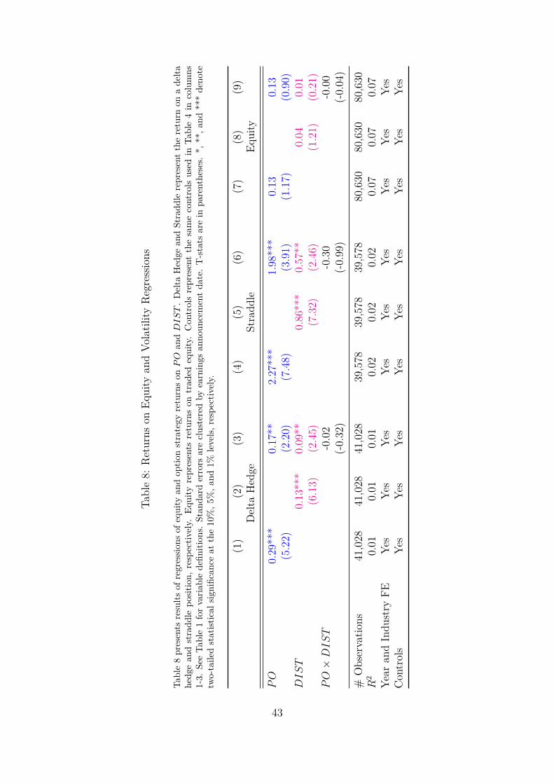
Tabl

e8:

Ret

urns

onEq

uity

and

Vola

tility

Reg

ress

ions

Tabl

e8

pres

ents

resu

ltsof

regr

essio

nsof

equi

tyan

dop

tion

stra

tegy

retu

rns

onP

Oan

dD

IS

T.

Del

taH

edge

and

Stra

ddle

repr

esen

tth

ere

turn

ona

delta

hedg

ean

dst

radd

lepo

sitio

n,re

spec

tivel

y.Eq

uity

repr

esen

tsre

turn

son

trad

edeq

uity

.C

ontr

ols

repr

esen

tth

esa

me

cont

rols

used

inTa

ble

4in

colu

mns

1-3.

See

Tabl

e1

for

varia

ble

defin

ition

s.St

anda

rder

rors

are

clus

tere

dby

earn

ings

anno

unce

men

tda

te.

T-s

tats

are

inpa

rent

hese

s.*,

**,a

nd**

*de

note

two-

taile

dst

atist

ical

signi

fican

ceat

the

10%

,5%

,and

1%le

vels,

resp

ectiv

ely.

(1)

(2)

(3)

(4)

(5)

(6)

(7)

(8)

(9)

Del

taH

edge

Stra

ddle

Equi

ty

PO

0.29

***

0.17

**2.

27**

*1.

98**

*0.

130.

13(5

.22)

(2.2

0)(7

.48)

(3.9

1)(1

.17)

(0.9

0)D

IS

T0.

13**

*0.

09**

0.86

***

0.57

**0.

040.

01(6

.13)

(2.4

5)(7

.32)

(2.4

6)(1

.21)

(0.2

1)P

O×

DIS

T-0

.02

-0.3

0-0

.00

(-0.

32)

(-0.

99)

(-0.

04)

#O

bser

vatio

ns41

,028

41,0

2841

,028

39,5

7839

,578

39,5

7880

,630

80,6

3080

,630

R2

0.01

0.01

0.01

0.02

0.02

0.02

0.07

0.07

0.07

Year

and

Indu

stry

FEYe

sYe

sYe

sYe

sYe

sYe

sYe

sYe

sYe

sC

ontr

ols

Yes

Yes

Yes

Yes

Yes

Yes

Yes

Yes

Yes

43

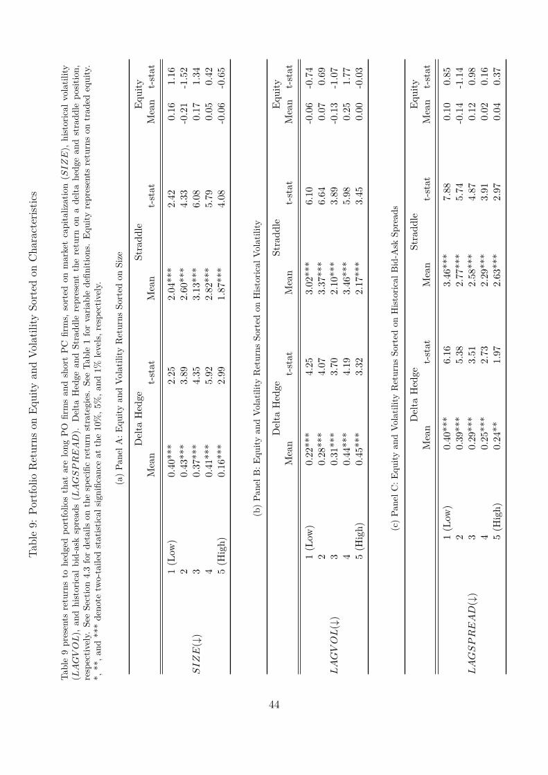
Tabl

e9:

Port

folio

Ret

urns

onEq

uity

and

Vola

tility

Sort

edon

Cha

ract

erist

ics

Tabl

e9

pres

ents

retu

rns

tohe

dged

port

folio

sth

atar

elo

ngPO

firm

san

dsh

ort

PCfir

ms,

sort

edon

mar

ket

capi

taliz

atio

n(S

IZ

E),

hist

oric

alvo

latil

ity(L

AG

VO

L),

and

hist

oric

albi

d-as

ksp

read

s(L

AG

SP

RE

AD

).D

elta

Hed

gean

dSt

radd

lere

pres

ent

the

retu

rnon

ade

ltahe

dge

and

stra

ddle

posit

ion,

resp

ectiv

ely.

See

Sect

ion

4.3

for

deta

ilson

the

spec

ific

retu

rnst

rate

gies

.Se

eTa

ble

1fo

rva

riabl

ede

finiti

ons.

Equi

tyre

pres

ents

retu

rns

ontr

aded

equi

ty.

*,**

,and

***

deno

tetw

o-ta

iled

stat

istic

alsig

nific

ance

atth

e10

%,5

%,a

nd1%

leve

ls,re

spec

tivel

y.

(a)

Pane

lA:E

quity

and

Vola

tility

Ret

urns

Sort

edon

Size

Del

taH

edge

Stra

ddle

Equi

tyM

ean

t-st

atM

ean

t-st

atM

ean

t-st

at

SIZ

E(↓

)

1(L

ow)

0.40

***

2.25

2.04

***

2.42

0.16

1.16

20.

43**

*3.

892.

60**

*4.

33-0

.21

-1.5

23

0.37

***

4.35

3.13

***

6.08

0.17

1.34

40.

41**

*5.

922.

82**

*5.

790.

050.

425

(Hig

h)0.

16**

*2.

991.

87**

*4.

08-0

.06

-0.6

5

(b)

Pane

lB:E

quity

and

Vola

tility

Ret

urns

Sort

edon

Hist

oric

alVo

latil

ity

Del

taH

edge

Stra

ddle

Equi

tyM

ean

t-st

atM

ean

t-st

atM

ean

t-st

at

LA

GV

OL

(↓)

1(L

ow)

0.22

***

4.25

3.02

***

6.10

-0.0

6-0

.74

20.

28**

*4.

073.

37**

*6.

640.

070.

693

0.31

***

3.70

2.10

***

3.89

-0.1

3-1

.07

40.

44**

*4.

193.

46**

*5.

980.

251.

775

(Hig

h)0.

45**

*3.

322.

17**

*3.

450.

00-0

.03

(c)

Pane

lC:E

quity

and

Vola

tility

Ret

urns

Sort

edon

Hist

oric

alB

id-A

skSp

read

s

Del

taH

edge

Stra

ddle

Equi

tyM

ean

t-st

atM

ean

t-st

atM

ean

t-st

at

LA

GS

PR

EA

D(↓

)

1(L

ow)

0.40

***

6.16

3.46

***

7.88

0.10

0.85

20.

39**

*5.

382.

77**

*5.

74-0

.14

-1.1

43

0.29

***

3.51

2.58

***

4.87

0.12

0.98

40.

25**

*2.

732.

29**

*3.

910.

020.

165

(Hig

h)0.

24**

1.97

2.63

***

2.97

0.04

0.37

44

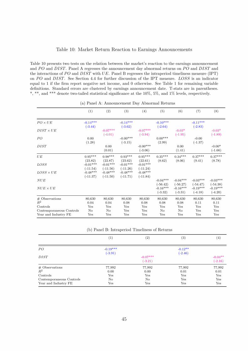
Table 10: Market Return Reaction to Earnings Announcements

Table 10 presents two tests on the relation between the market’s reaction to the earnings announcementand PO and DIST . Panel A regresses the announcement day abnormal returns on PO and DIST andthe interactions of PO and DIST with UE. Panel B regresses the intraperiod timeliness measure (IPT)on PO and DIST . See Section 4.4 for further discussion of the IPT measure. LOSS is an indicatorequal to 1 if the firm report negative net income, and 0 otherwise. See Table 1 for remaining variabledefinitions. Standard errors are clustered by earnings announcement date. T-stats are in parentheses.*, **, and *** denote two-tailed statistical significance at the 10%, 5%, and 1% levels, respectively.

(a) Panel A: Announcement Day Abnormal Returns

(1) (2) (3) (4) (5) (6) (7) (8)

P O × UE -0.14*** -0.14*** -0.10*** -0.11***(-3.44) (-3.62) (-2.64) (-2.83)

DIST × UE -0.07*** -0.07*** -0.03* -0.03*(-4.01) (-3.94) (-1.95) (-1.89)

P O 0.00 -0.00*** 0.00*** -0.00(1.28) (-3.15) (2.99) (-1.37)

DIST 0.00 -0.00*** 0.00 -0.00*(0.01) (-3.06) (1.41) (-1.66)

UE 0.95*** 0.98*** 0.93*** 0.95*** 0.35*** 0.34*** 0.37*** 0.37***(23.82) (22.87) (23.62) (22.61) (8.62) (8.06) (9.41) (8.78)

LOSS -0.01*** -0.01*** -0.01*** -0.01***(-11.54) (-11.56) (-11.26) (-11.24)

LOSS × UE -0.48*** -0.48*** -0.48*** -0.48***(-11.37) (-11.50) (-11.71) (-11.84)

NUE -0.04*** -0.04*** -0.03*** -0.03***(-56.42) (-56.27) (-54.47) (-54.38)

NUE × UE -0.16*** -0.16*** -0.19*** -0.19***(-3.32) (-3.31) (-4.18) (-4.20)

# Observations 80,630 80,630 80,630 80,630 80,630 80,630 80,630 80,630R2 0.04 0.04 0.08 0.08 0.08 0.08 0.11 0.11Controls Yes Yes Yes Yes Yes Yes Yes YesContemporaneous Controls No No Yes Yes No No Yes YesYear and Industry FE Yes Yes Yes Yes Yes Yes Yes Yes

(b) Panel B: Intraperiod Timeliness of Returns

(1) (2) (3) (4)

P O -0.19*** -0.12**(-3.91) (-2.46)

DIST -0.07*** -0.04**(-3.21) (-2.16)

# Observations 77,992 77,992 77,992 77,992R2 0.00 0.00 0.01 0.01Controls Yes Yes Yes YesContemporaneous Controls No No Yes YesYear and Industry FE Yes Yes Yes Yes

45