Volatility as Investment - Crash Protection with … as Investment - Crash Protection with Calendar ... both negative risk premium and ... decreases linearly with time as a direct

Volatility as Investment -Crash Protection with Calendar Spreads of Variance

Swaps∗

Uwe WystupMathFinance AG

[email protected]

Qixiang ZhouFrankfurt School of Finance & Management

[email protected]

25 July 2014

Abstract

Nowadays, volatility is not only a risk measure but can be also considered anindividual asset class. Variance swaps, one of the main investment vehicles, can ob-tain pure exposure on realized volatility. In normal market phases, implied volatilityis often higher than the realized volatility will turn out to be.

In this paper, we show a volatility investment strategy which can benefit fromboth negative risk premium and correlation of variance swaps to the underlyingstock index. The empirical evidence demonstrate a significant diversification effectduring the financial crisis by adding this strategy to the equity portfolio. Theback testing analysis includes the last ten years of history of the S&P500 and theEUROSTOXX50.

∗We thank Nils Detering for his contribution a previous German version of this paper, Julia Weinhardtfor proof-reading the English version and Lupus alpha for supporting the research work.

1

mailto:[email protected]

mailto:[email protected]

Volatility as Investment 2

1 Introduction

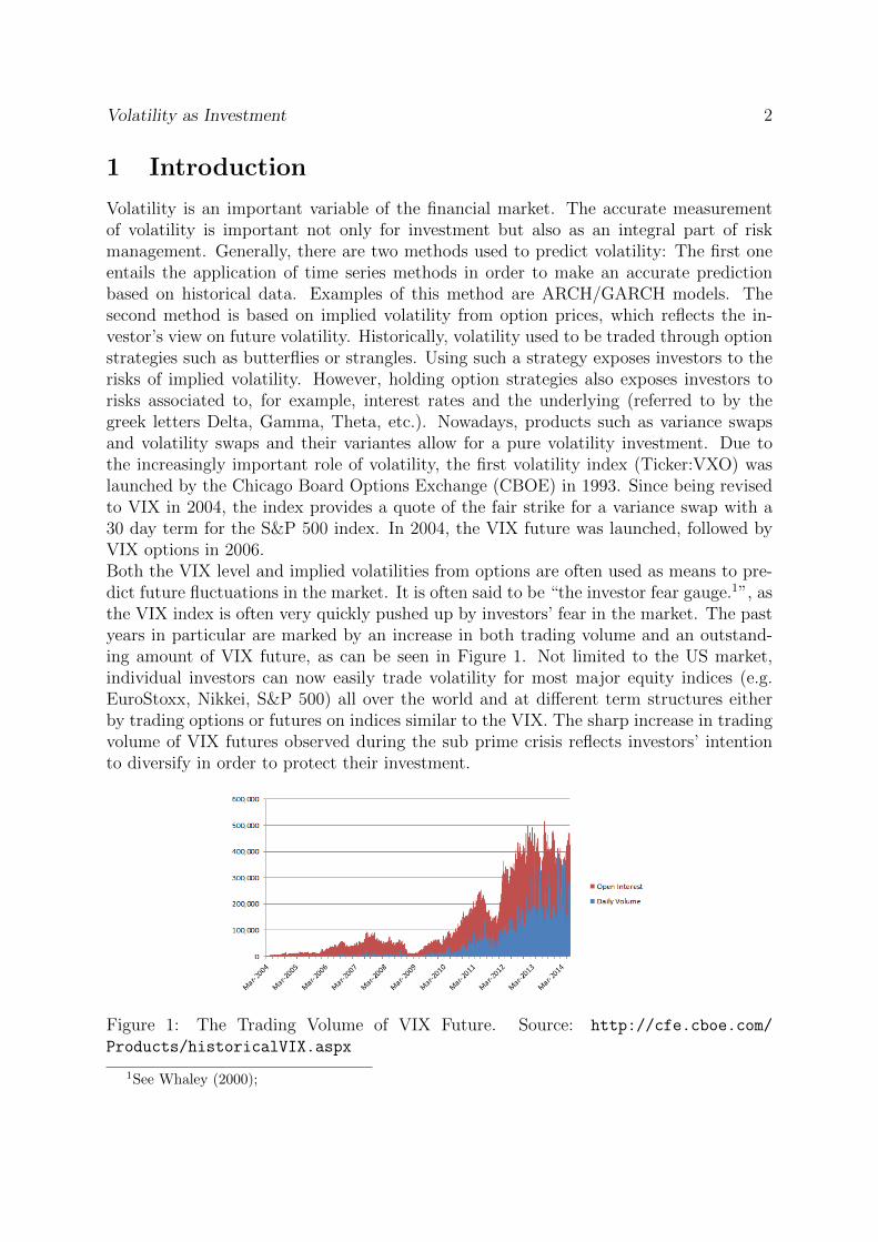
Volatility is an important variable of the financial market. The accurate measurementof volatility is important not only for investment but also as an integral part of riskmanagement. Generally, there are two methods used to predict volatility: The first oneentails the application of time series methods in order to make an accurate predictionbased on historical data. Examples of this method are ARCH/GARCH models. Thesecond method is based on implied volatility from option prices, which reflects the in-vestor’s view on future volatility. Historically, volatility used to be traded through optionstrategies such as butterflies or strangles. Using such a strategy exposes investors to therisks of implied volatility. However, holding option strategies also exposes investors torisks associated to, for example, interest rates and the underlying (referred to by thegreek letters Delta, Gamma, Theta, etc.). Nowadays, products such as variance swapsand volatility swaps and their variantes allow for a pure volatility investment. Due tothe increasingly important role of volatility, the first volatility index (Ticker:VXO) waslaunched by the Chicago Board Options Exchange (CBOE) in 1993. Since being revisedto VIX in 2004, the index provides a quote of the fair strike for a variance swap with a30 day term for the S&P 500 index. In 2004, the VIX future was launched, followed byVIX options in 2006.Both the VIX level and implied volatilities from options are often used as means to pre-dict future fluctuations in the market. It is often said to be “the investor fear gauge.1”, asthe VIX index is often very quickly pushed up by investors’ fear in the market. The pastyears in particular are marked by an increase in both trading volume and an outstand-ing amount of VIX future, as can be seen in Figure 1. Not limited to the US market,individual investors can now easily trade volatility for most major equity indices (e.g.EuroStoxx, Nikkei, S&P 500) all over the world and at different term structures eitherby trading options or futures on indices similar to the VIX. The sharp increase in tradingvolume of VIX futures observed during the sub prime crisis reflects investors’ intentionto diversify in order to protect their investment.

Figure 1: The Trading Volume of VIX Future. Source: http://cfe.cboe.com/

Products/historicalVIX.aspx

1See Whaley (2000);

http://cfe.cboe.com/Products/historicalVIX.aspx

http://cfe.cboe.com/Products/historicalVIX.aspx


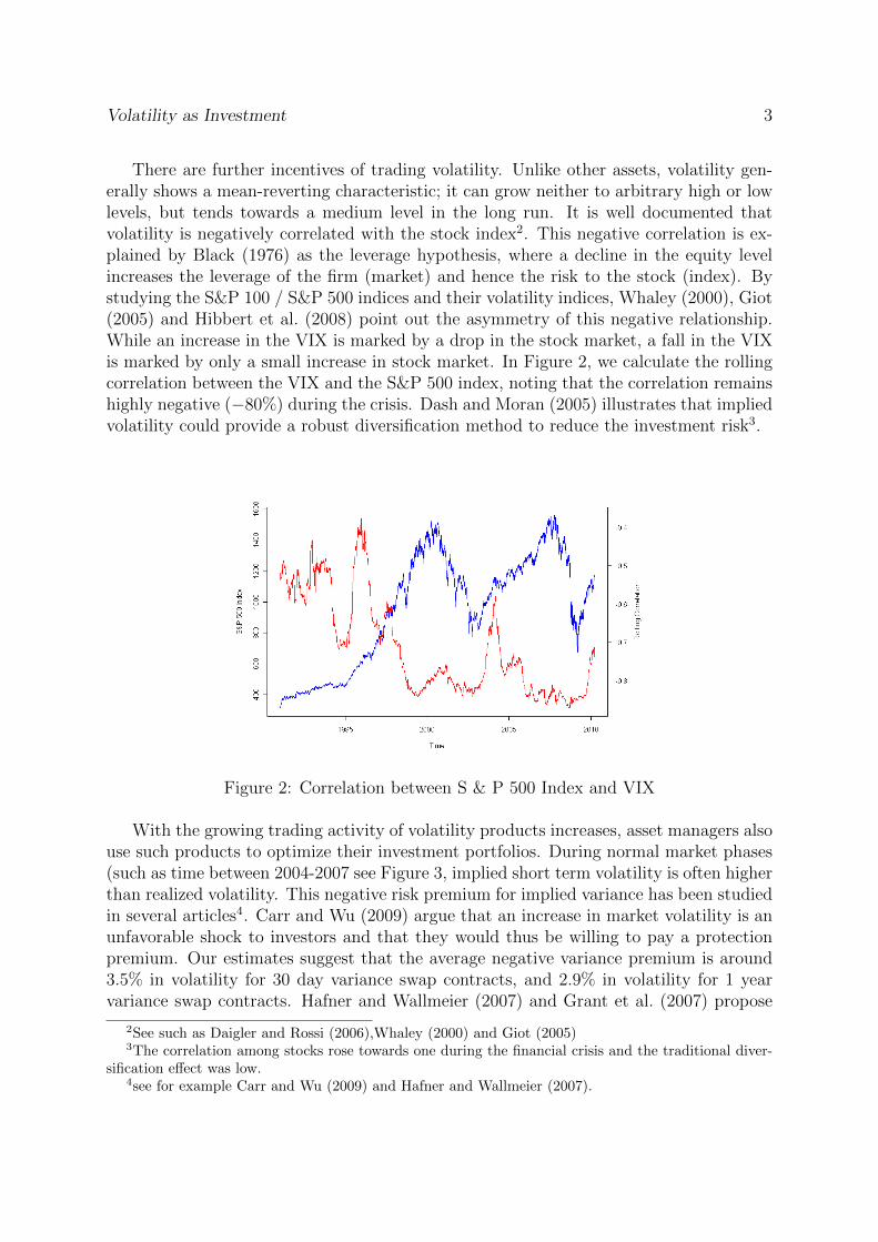
There are further incentives of trading volatility. Unlike other assets, volatility gen-erally shows a mean-reverting characteristic; it can grow neither to arbitrary high or lowlevels, but tends towards a medium level in the long run. It is well documented thatvolatility is negatively correlated with the stock index2. This negative correlation is ex-plained by Black (1976) as the leverage hypothesis, where a decline in the equity levelincreases the leverage of the firm (market) and hence the risk to the stock (index). Bystudying the S&P 100 / S&P 500 indices and their volatility indices, Whaley (2000), Giot(2005) and Hibbert et al. (2008) point out the asymmetry of this negative relationship.While an increase in the VIX is marked by a drop in the stock market, a fall in the VIXis marked by only a small increase in stock market. In Figure 2, we calculate the rollingcorrelation between the VIX and the S&P 500 index, noting that the correlation remainshighly negative (−80%) during the crisis. Dash and Moran (2005) illustrates that impliedvolatility could provide a robust diversification method to reduce the investment risk3.

Figure 2: Correlation between S & P 500 Index and VIX

With the growing trading activity of volatility products increases, asset managers alsouse such products to optimize their investment portfolios. During normal market phases(such as time between 2004-2007 see Figure 3, implied short term volatility is often higherthan realized volatility. This negative risk premium for implied variance has been studiedin several articles4. Carr and Wu (2009) argue that an increase in market volatility is anunfavorable shock to investors and that they would thus be willing to pay a protectionpremium. Our estimates suggest that the average negative variance premium is around3.5% in volatility for 30 day variance swap contracts, and 2.9% in volatility for 1 yearvariance swap contracts. Hafner and Wallmeier (2007) and Grant et al. (2007) propose

2See such as Daigler and Rossi (2006),Whaley (2000) and Giot (2005)3The correlation among stocks rose towards one during the financial crisis and the traditional diver-

sification effect was low.4see for example Carr and Wu (2009) and Hafner and Wallmeier (2007).


to add an exclusive variance swap selling strategy to a portfolio in order to earn thispremium. However, a strategy based exclusively on selling does not make use of the neg-ative correlation between the variance swaps and the underlying asset, thus rendering thediversification effect trivial. Szado (2009) points out that a long volatility strategy wouldsignificantly help investors to diversify and protect their portfolio during the financialcrisis. However, he does admit that this would be an expensive means of protection as itcauses negative returns during normal market phases.

Figure 3: Negative Premium of Variance Swaps

In this study, complementing existing research, we introduce a trading strategy ofimplied volatility that provides diversification at almost zero cost. We use the idea ofcalendar spreads from option trading and apply it to variance swaps. A calendar spreadof variance swaps combines selling short term and buying long term variance swaps. Thisstrategy can avoid the high costs encountered in single buying strategies and the lowdiversification effects in simple selling strategies. The key idea here lies in buying thevariance swaps with long maturities at low frequencies while selling short term swaps ata higher frequency. At each trading point, we weigh the long term contract with a muchhigher notional than the short term ones in order to maintain a net zero vega. In theempirical study part, we use original broker quotes for 1, 3, 6 and 12 month varianceswaps between 2004 and 2011. We assume our original investment portfolio to consist of70% S&P 500 and 30% fixed income investment. We apply a calendar spread of buying1 year and selling 1 month variance swaps to diversify the portfolio. Our estimates showthat the addition of this strategy raises the mean return of the original portfolio by around250%, while reducing the realized portfolio volatility to 50% of the original portfolio’svolatility.


The remaining paper is organized as follows: Section 2 briefly introduces the valuationmodel of variance swaps and Section 3 analyzes the performance of trading single varianceswaps. In Section 4, the calendar spread settings are introduced and we present theperformance of a predefined case. Further, we expand the strategy to different weightsand illustrate more general cases of performance. We will show the robustness of uing acalendar spread by shifting the trading dates in Section 5. We conclude in Section 6.

2 Empirical Study Setup

Variance swaps started to be traded in the late 1980s as an over-the-counter (OTC)derivative paying the difference between the realized variance σ2

R and the predefinedimplied variance or strike σ2

K . Usually the strike σ2K is determined such that the initial

value of the swap is zero. The variance swap can be replicated by trading a series ofout-of-the-money (OTM) call and put options. The term of a variance swap contract istaken to be 1 month (30 days) and 1 year (365 days) in our study. The fair strike σK is theimplied volatility, as determined at the beginning of the contract. For simplicity, if theend of a variance swap is not a business day, the settlement of the variance swap contractis adjusted to be the last business day over the duration period of the study. Generally,variance swap contracts are measured in dollar notional (Notional). In our empiricalstudy, we will use fix leg payments (or “DollarAmount”) to measure the weights of thevariance swaps. The relationship between notional and dollar amount is given by

DollarAmount = Notional · σ2K . (1)

We denote Vega exposure of variance swaps as Vegat. It calculates as Vegat = 2·Notional·σK . The vega exposure will be positive if we buy implied volatility and negative if wesell. The contract ends with a cash payment at maturity, determined by the formula

Payoff = Notional · (σ2R − σ2

K). (2)

Here, the realized volatility σR is calculated by

σR =

√√√√252

N

N∑i=1

(xi)2 · 100. (3)

The return is a daily log return xi = ln Si

Si−1and N is the number of business days within

the contract. The mark-to-market value of a variance swap at any time t ∈ (0, T ) is theweighted sum of realized variance and implied variance,

Pricet = Notional× PVt(T )

[t

T(σR(0, t))2 +

T − tT

(σim(t, T ))2 − σ2K

](4)

Here, the PVt(T ) is the present value at time t of receiving 1$ at maturity T . And σR(0, t)is the realized volatility until time t and σim(t, T ) is the implied volatility from time t to


maturity. In our study, the σim(t, T ) is determined by linear interpolation. The inputsare implied volatilities for term structures with maturity of 1 month, 3 month, 6 monthand 1 year. We use the 1 month implied volatility for any implied volatility that is shorterthan 30 days and apply a linear interpolation to calculate σimplied(t, T ) in other cases as

σimplied(t, T ) = impV olt1 + (T − t− t1) ·impV olt2 − impV olt1

t2 − t1, (5)

where t1, t2 is the time interval that T − t belongs to and impV olt1 , impV olt2 are thecorresponding implied volatilities. The sensitivity of a variance swap to implied volatilitydecreases linearly with time as a direct consequence of mark-to-market additivity and isgiven by

Vega =δPricetδσimplied

= Notional · (2 · σimplied) ·T − tT

. (6)

Here, the σimplied is the implied volatility until contract maturity, t is the valuation timeand T is the maturity.

3 Single Variance Swap Strategy

We assume our underlying portfolio to be a mix of 70% of S&P 500 index and 30% fixedincome investment with an initial value of $1 Million. In the first part of empirical studywe want to demonstrate the diversification effect by adding a single variance swap tothat 70-30 portfolio. We consider the time interval from January 2004 to June 20115,which covers the sub-prime crisis. Further, we use short term (1 month) or long term(12 month) variance swaps. We focus on the daily log change of the stock index andimplied volatility. We present basic statistics concerning their features in Table 1, andfind that both indices show non-normal characteisticss due to their high kurtosis. Weshould expect an extreme fat tail in the distribution of implied volatility.

Mean Return Volatility Skew KurtosisVarSwap 1M 0.00% (-0.46% p.a.) 6.59% (104.68% p.a.) 0.59 4.03VarSwap 1Y 0.02% (4.37% p.a.) 2.43% (38.61% p.a.) 0.53 4.38

Table 1: Summary statistics

In total, there are four scenarios in which we add a single variance swap to a portfolio- namely by selling or buying 1 month/1 year variance swaps. In our study, we assumeno transaction costs and the portfolio to be rebalanced at a weekly frequency. FromEquation (5), we see that the vega exposure of a variance swap decays linearly with time.In order to maintain a more stable vega exposure, we need to trade a variance swap ata frequency that allows the contracts to overlap each other. Considering the possibletransaction costs in practice, we set the trading frequency to be approximately 1

4of the

5In this time series we only use the business days on which all quotes are available.


tenor. We then have four contracts overlapping each other at any valuation point. So fora 1 month variance swap, we assume it to be traded weekly 6. The trading frequency for a1 year contract is quarterly 7. Another important issue is how to manage the notional ofthe variance swap. If we measure the weights by notional, the vega exposure will have apositive relationship with the prevailing implied volatility. This in turn would cause morevega risk in turbulent markets than at any other time. In general, a high risk exposureduring the financial crisis is not a preferable situation for the investor. Consequently, wepropose to use a dollar amount (Equation 1) to manage the notional. When we fix thetotal dollar amount, we will trade much more notional of variance swap during normalmarket phases than during turbulence. This dynamic notional management is in linewith most investors’ preference. Considering the portfolio value of 1 million, we set thedollar amount to be 7500$ for 1 month variance swap at each trading point and 50, 000$for 1 year variance swap. In order to measure the portfolio performance as well as thepotential risks, we use three risk adjusted measures: the Sharpe ratio, Kappa 1 (known asSortino Ratio) and Kappa 2 (known as Omega Ratio). The results of different portfoliosare presented in Table 2 and the cumulative returns are shown in Figure 5.

Mean Return Volatility Sharpe Ratio Kappa 1 Kappa 270/30 Strategy 3.72% 14.70% 0.1476 14.03 5.55Selling VarSwap 1M 9.49% 17.98% 0.4417 29.17 10.74Buying VarSwap 1M -6.65% 12.26% -0.6686 -25.4765 -14.2876Selling VarSwap 1Y 4.18% 45.35% 0.0579 7.8531 1.9065Buying VarSwap 1Y 3.25% 10.24% 0.1656 17.7183 8.4176

Table 2: Single Variance Swap Strategy

With respect to the selling strategy, we realized similar results as Hafner and Wall-meier (2007) and Grant et al. (2007).

The premium we earn from the selling strategy significantly increases the portfolio’smean return. Through the weekly selling of a 1 month variance swap, the portfolio’smean return rises by more than 250% while the volatility only increases by less than25%. Therefore, we observe much better risk-adjusted performance measures for theportfolio. However, when we look at the cumulative return in Figure 5 between 2008and 2009, rather than provide protection during the crisis, selling variance swaps furtherpushes down the portfolio’s return. This does not favor investors looking to diversifywith volatility.When it comes to the buying strategy, the volatility of the new portfolio is significantlylower than the original one. During the financial crisis, the variance swap provides pro-tection to the investor and we can not find a significant drop in the total portfolio returnsin the buying strategy. However, a high risk premium paid to protect the market from

6We assume that a variance swap is traded on each Monday. If Monday is not a business day thenwe move to the next possible business day.

7We assume that a variance swap is traded on the first day of the months January, April, July andOctober. If that day is not a business day then we move to the next possible business day.


crashing sharply results in a reduction of mean return from the investment. The premi-ums of buying variance swaps are even higher than the total returns from the index. Inthe case of buying a 1 month contract we even have a highly negative return at −6.65%per year.

Figure 4: Single Variance Swap Strategy

4 Calendar Spread Strategy

In the last section, we demonstrated the performance achieved when adding single vari-ance swaps to a traditional portfolio. The shortcomings of these strategies are obvious.The selling strategy does not benefit from the diversification and buying one is too ex-pensive to be carried out in a normal market phase. We estimated that the averagenegative premiums of 1 month and 1 year variance swaps are −51.65 and −46.06 pernotional. We can consider the expected marginal cost of buying 1 notional variance swapto be approximately 50$. If we supposedly want to offer crash protection to the portfo-lio incase of an increase in volatility, we need to retain a positive vega in our varianceswap strategy. Therefore, a long variance swap would be our only choice. This wouldbe expensive and we want to reduce the risk premium. It is not difficult to find that wecan sell the variance swaps at the same time to earn a similar amount of risk premiumas compensation. Further, the correlation between the movement of 1 month and 1 yearimplied volatility is strong at 84.56%. We could expect a similar implied volatility curvemovement from this high correlation. In practice, a derivatives trader uses a calendarspread to benefit from this parallel volatility curve movement. In the simplest case, webuy a 1 year variance swap and sell a 1 month contract with 1 notional each day. The


expected risk premium to be paid on the 1 year swap could be compensated by selling the1 month swap. Thus, by using a calendar spread structure, we provide a strategy withalmost zero expected risk premium. After 1 month the sold contract will expire and thebought 1 year variance swap could provide protection to the portfolio for the remaining11 months. Within the first month, we hold both, the short and the long contract. FromTable 1, we know that the volatility of the 1 month implied volatility is about 2.5 timesof the 1 year implied one. Therefore, if we want to offset the returns of a variance swapcalendar spread, we need to keep the vega exposure for the long one to be 2.5 times higherthan for the short one. It is not very difficult to solve this problem. We can expand theidea above to buying a 1 year variance swap today and selling a 1 month contract in thesecond month and repeat this for the third month. We combine three simple strategiesand now buy 3 times the notional of 1 year variance swaps at the beginning while sellinga 1 notional swap on the first day of every month for the next three months. We cankeep the vega exposure for the long position to be 2.5 times or more than for the shortposition. Finally, the expected premium of the long and shot variance swaps offset eachother and within the first three months, the return on the two contracts would be welldiversified and we get full protection for the remaining 9 months. We can repeat thisstrategy every quarter and the overlapping strategy would give reasonable protection tothe portfolio. So far, we have constructed a calendar spread to provide crash protectionto the stock portfolio at almost no cost. The key idea of the calendar spread could besummarized as,

1. We need to have two variance swaps at different maturities;

2. A long position is held for variance swaps with longer maturity and short for theother one;

3. At each trading point, we trade more notional in the long term swaps than in theshort term one;

4. We need to sell variance swaps at a higher frequency to match the total notional ofthe long position;

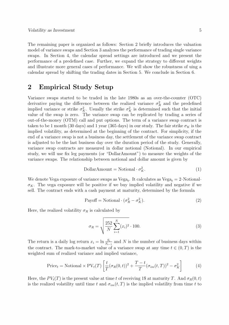
We will now demonstrate a more general case. Coming back to the example of the singlestrategy in the last section. We buy a 50, 000$ 1 year swap quarterly and sell a 7, 500$1 month variance swap contract on a weekly basis. Theoretically, we have four contractsoverlapping each other. By estimation, we hold 200, 000$ in long variance swaps whileholding 30, 000$ in short variance swaps at any time. The vega difference between thelong and short strategy is shown as the blue line in Figure 5. If we now combine thesetwo single strategies, the resulting strategy matches the key idea of a calendar spreadfor variance swaps. In each calender year, we could estimate to sell 360, 000$ of varianceswaps which is greater than the 200, 000$ buying amount. We are actually earning pre-mium in this situation.We show the results of the calendar spread variance swap strategy8. Figure 5 shows the

8As there is no initial investment for the variance swap, we add 1 million dollar cash to the strategyto calculate the performance of this calendar spread.


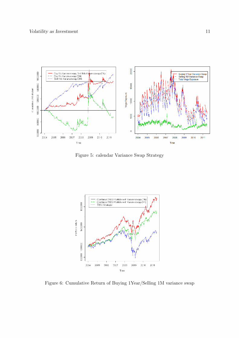
cumulative return of this strategy and Table 3 presents a summary of the statistics.In Figure 5, we show cumulative returns of the exclusive short strategy (blue line), longstrategy (green line) and calendar spread (red line). Prior to 2008, unlike the portfoliovalue of the buy strategy which falls below the initial value, our calendar spread actuallygenerates positive returns. When the financial crisis hits in 2008, the calendar spreadjumps upward while the value of the short strategy drops heavily. The calendar spreadreaches the highest risk adjusted performance in Kappa 1 and Kappa 2. Unlike the neg-ative mean return of the 1 year strategy, it has a significant positive return of 5.43% inour case, which is only about 1% lower than the sell strategy. Finally, we estimate thatthe correlation between calendar spread and our underlying portfolio is around −79.70%.Recognizing the advantages of the combined calendar spread, we now want to add itto the portfolio to analyze the extent to which the performance can be improved. Wepresent the cumulative returns of the combined portfolio in Figure 6 and summarizingstatistics in Table 4. By adding the calendar spread to the 70-30 portfolio, we successfullyincrease the return from 3.72% to 9.19% while reducing the volatility to 9.63% by almost5%. We get a Sharpe ratio which is 5 times greater than in the original portfolio, and 2-3times greater in Kappa 1 and Kappa 2 measures. As we can see from Figure 6, during2008 the down side drop is significantly reduced by the variance swap. In the densityplot shown in Figure 7, we can clearly see that the combined strategy is skewed to theright and that the down side tail distribution is rather small. The density has shiftedto the right from the original distribution significantly. In Table 5, we show some riskmeasures at the extreme condition. By adding a calendar spread, the minimum returnand high quantile VaR are significantly reduced. We have thus successfully used twovariance swaps with different maturities to construct a calendar spread strategy whichcorrelates highly negatively with the stock index while no or even positive premium isearned.

Strategy Selling 1-Month Buying 1-Year CombinedMean 6,59% -1,70% 5,43%Volatility 5,08% 21,61% 10,28%Sharpe Ratio 1,2975 -0,0787 0,5284Kappa 1 29.17 17.7183 49.0037Kappa 2 10.74 8.4176 20.7640

Table 3: Buying 1 Year, Selling 1 Month variance swap strategy

Taking this idea further, we will weigh a 1Y and a 1M variance swaps differentlyusing the calendar spread strategy. As we know, the portfolio value changes with marketfluctuation. A fixed notional would thus not be a good choice with regards to portfoliomanagement. We adjust the notional when buying a 1Y contract to be a percentage ofthe total portfolio value. As we sell a 1M contract at a smaller amount but at a higherfrequency each time, we weigh the dollar amount sold as a proportion of the 1 year vari-ance swap notional. We set the minimum amount of buying a 1Y variance swap to be


Figure 5: calendar Variance Swap Strategy

Figure 6: Cumulative Return of Buying 1Year/Selling 1M variance swap


S&P 500 JPM 70/30 Strat. Combined (DN)Mean Return 2, 52% 5, 29% 3, 72% 9,19%Volatility 21, 40% 4, 07% 14, 70% 9,63%Sharpe Ratio 0,0441 0,9178 0,1475 0,7924Kappa 1 14.03 49.0037Kappa 2 5.55 20.7640

Table 4: Statistic Character of Portfolios

Min VaR 99% VaR 99.9%70/30 Strat. −6.54% −6.21% −2.90%Combined −5.36% −3.58% −1.78%

Table 5: Risk measures of Portfolio

1% of the total portfolio value and cap the maximum amount at 10%. The 1M varianceswap would have a weight of 5% compared to 10% of the 1Y notional.

We present all results in Figure 8. If we fix the weights of the 1M notional, we see thatthe Sharpe ratio is a concave function of the 1Y notional. If we only buy a small amountof 1Y variance swaps, it can not provide enough protection during the crisis. However,if the weight a 1Y contract too much, the portfolio would not peform well due to thehigh premium paid when buying variance swaps. It is thus very important to determinesuitable weights for the 1Y variance swap. The portfolio volatility is a convex function ofthe weights of a 1Y contract. The diversification effect is most significant when buying3%-4% 1Y variance swaps. In summary, weighting 1Y variance swaps at 3%-4% of thetotal portfolio value would be a good choice, as this strategy provides both a high Sharperatio and the desired diversification effect.

If we fix the amount of long 1Y contracts and sell a larger number of 1M contracts, thiswould always give us a positive marginal change of the portfolio Sharpe ratio. However,the speed at which it increases would decrease if we weigh them at more than 20% of thelong amount. The volatility of the portfolio does not change significantly when we raisethe weights of the sold notional. We should observe the effect on the Sharpe ratio. As westated before, selling single variance swaps would increase the Sharpe ratio but aggregatethe loss in the financial crisis. This is why it is important for us to find the right ratio.The figure shows that we can expect a 1Y notional in the range of 15%-20% to give usthe best portfolio performance.

5 Robustness of the Strategy

We have seen the significant performance improvement achieved through trading a cal-endar spread variance swap strategy. However, we assume that the trading occurrs onsome specific date. One would argue that the strategy might not work well if we shift


Figure 7: Kernel Density of Combined Portfolio

Figure 8: Surface of Sharpe Ratio and Volatility at Different Weight scheme


the trading date. We now want to show the robustness of this calendar spread strategyin the face of a change in dates. We maintain the same trading frequency, but choose adifferent starting date. For the single 1M strategy, we will show the results if we tradefrom every Monday to Friday 9 And for selling the 1Y strategy, we shift the starting dateby five business days (Weekly). All the results are presented in Table 6 and Table 7.For the selling 1M strategy, we always reach a Sharpe ratio greater than 0.8, in mostcases, a Sharpe ratio greater than 1. Similarly, the Sharpe ratio of selling 1Y contractsis always positive. We consider the difference between different Sharpe ratios within anacceptable range. We get similar results when shifting trading days of variance swapson the EuroStoxx index. The variance swap maintains its own characteristic throughouttime.

Day 0 1 2 3 4Mean Return p.a. 4.78% 4.34% 5.05% 5.46% 5.69%Sharpe Ratio p.a. 1.0154 0.8868 1.1158 1.2181 1.2420Difference in % 0.00% -19.78% 0.94% 10.20% 12.36%Here, 0-4 corresponds to Monday-Friday;

Table 6: Trading Day Shift of 1M Strategy

Week 0 1 2 3 4 5Mean Return p.a. 2.15% 2.35% 2.35% 2.08% 2.05% 1.86%Sharpe Ratio p.a. 0.1069 0.1269 0.1324 0.1078 0.1090 0.0921Difference in % 0.00% 18.78% 23.89% 0.86% 1.99% -13.80%Week 6 7 8 9 10 11Mean Return (USD) 1.70% 1.75% 2.02% 1.57% 1.80% 1.92%Sharpe Ratio p.a. 0.0837 0.0868 0.0999 0.0720 0.0874 0.0895Difference in % -21.66% -18.79% -6.54% -32.66% -18.18% -16.28%Week 12Mean Return (USD) 2.42%Sharpe Ratio p.a. 0.1220Difference in % 14.17%

Table 7: Trading Day Shift of 1Y Strategy

6 Conclusion

In this paper, we show the different characteristics of variance swaps. In the post crisistime, the implied volatility remains at a high level while the market is recovering and hasa much smaller realized volatility. We also find that, by selling single variance swaps, one

9If a given date is not a business day, we shift them to the day after.


can improve the Sharpe ratio of the portfolio by achieving a much higher mean return.However, a pure selling strategy would also leverage the loss during the financial crisisand would not provide any diversification effect to the portfolio. We analyze a calendarspread strategy that consists of buying long term variance swaps and selling short termcontracts at a higher frequency.

In a backtest we analyse a calendar spread strategy trading variance swaps to avoidthe shortcomings encountered when trading single variance swap contracts. Ignoring bid-offer spreads, this calendar spread strategy gives us good protection from potential marketcrashes at almost zero or even negative costs. The combined strategy can maintain acorrelation of almost −80% to the original portfolio, providing a noticeable diversificationeffect. We show that the volatility of a 70-30 equity-bond portfolio would decrease from14.70% to 9.63% while the mean return would increase from 3.72% to 9.19%. Besidesthat, the calendar spread also greatly reduces the tail risk at a higher quantile. The lossat the 0.1% and 1% quantile would be less than 60% of the original portfolio. Finally, welink the notional of a variance swap to the portfolio value. We suggest that buying 1Yvariance swaps at 3 − 4% of the total value and selling 1M variance swaps at 15 − 20%to the 1Y notional would provide the best performance of the calendar spread strategy.

Finally, we would like to point out that the results are based on a backtesting analysisand have no automatic predicitive power. For example, the strategy may perform badlyin the future in case of a linear (zero variance) asset melt-down.

References

Black, F. (1976). Studies of stock price volatility changes. In Proceedings of the 1976Meetings of the American Statistical Association, Business and Economics StatisticsSection, pages 177–181.

Carr, P. and Wu, L. (2009). Variance risk premiums. Review of Financial Studies,22(3):1311–1341.

Daigler, R. T. and Rossi, L. (2006). A portfolio of stocks and volatility. The Journal ofInvesting, 15:99–106.

Dash, S. and Moran, M. T. (2005). Vix as a companion for hedge fund portfolios. TheJournal of Alternative Investments, 8:75–80.

Giot, P. (2005). Relationships between implied volatility indexes and stock index returns.The Journal of Portfolio Management, 31(3):92–100.

Grant, M., Gregory, K., and Lui, J. (2007). Volatility as an asset. Goldman Sachs StrategyResearch.

Hafner, R. and Wallmeier, M. (2007). Volatility as an asset class: European evidence.European Journal of Finance, 13(7):621–644.


Hibbert, A. M., Daigler, R. T., and Dupoyet, B. (2008). A behavioral explanation forthe negative asymmetric return-volatility relation. Journal of Banking & Finance,32(10):2254–2266.

Szado, E. (2009). Vix futures and options a case study of portfolio diversification duringthe 2008 financial crisis. CBOE Research Paper.

Whaley, R. E. (2000). The investor fear gauge. Journal of Portfolio Management, 26:12–17.

Documents

Volatility as Investment - Crash Protection with … as Investment - Crash Protection with Calendar ... both negative risk premium and ... decreases linearly with time as a direct