Embed Size (px)
Citation preview

Sponsored by the Department of Science and Technology
Volume 27 Number 3 • August 2016

SubmissionsIt is the policy of the Journal of Energy in Southern Africa topublish papers covering the technical, economic, policy,environmental and social aspects of energy research anddevelopment carried out in, or relevant to, Southern Africa.Only previously unpublished work will be accepted;conference papers delivered but not published elsewhereare also welcomed. Short comments, not exceeding 500words, on articles appearing in JESA are invited. Relevantitems of general interest, news, statistics, technical notes,reviews and research results will also be included, as willannouncements of recent publications, reviews,conferences, seminars and meetings. Those wishing to submit contributions should refer to theguidelines given on the JESA website (although these arecurrently under review). The Editorial Committee does not accept responsibility forviewpoints or opinions expressed here, or the correctnessof facts and figures.
The Journal of Energy in South Africa is accredited by theSouth African Department of Higher Education and Trainingfor university subsidy purposes. It is abstracted and indexedin Environment Abstract, Index to South African Periodicals,and the Nexus Database System. JESA has also beenselected into the Science Citation Index Expanded byThomson Reuters (as from Volume 19 No 1). It is also onthe Scientific Electronic Library Online SA platform and ismanaged by the Academy of Science of South Africa.
The Editorial Committee does not accept responsibility forviewpoints or opinions expressed here, or the correctnessof facts and figures.
Website: www.erc.uct.ac.za/journals/jesa
© Energy Research Centre ISSN 1021 447X
Scholarly Managing EditorMokone Roberts
Editorial board Kornelis Blok Ecofys Consultancy Group, Utrecht, The Netherlands
Anton Eberhard UCT Graduate School of Business, Cape Town, South Africa
Roula Inglesi-Lotz University of Pretoria, Pretoria, South Africa
Gilberto M. Jannuzzi University of Campinas, São Paulo, Brazil
Daniel Kammen University of California, Berkeley, USA
Jiang Ke Jun Energy Research Institute, China
Barry MacColl Eskom, Pretoria, South Africa
Yacob Malugetta University College, London, UK
Nthabiseng Mohlakoana University of Twente, Enschede, Netherlands
Angela Cadena Monroy Mining Planning Unit Energy, Colombia
Velaphi Msimang Mapungubwe Institute for Strategic Reflection,Johannesburg, South Africa
Anand Patwardhan Indian Institute of Technology, Bombay, India
Ambuj Sagar Indian Institute of Technology, Delhi, India
Wikus Van Niekerk Stellenbosch University, Stellenbosch, South Africa
Francis Yamba University of Zambia, Lusaka, Zambia
Sponsored by the Departmentof Science & Technology

CONTENTS
1 Promoting energy efficiency in a South African university Nandarani Maistry, Tracey Morton McKay
11 Scoping exercise to determine load profile archetypereference shapes for solar co-generation models inisolated off-grid rural African villages Gerro Prinsloo, Robert Dobson, Alan Brent
28 Varying percentages of full uniform shading of a PV module in a controlled environment yields linearpower reductionArthur James Swart, Pierre E. Hertzog
39 Determination of oxidation characteristics anddecomposition kinetics of some Nigerian biomassEC Okoroigwe, SO Enibe, SO Onyegegbu
50 Ranking South African provinces on the basis of MERRA2D surface incident shortwave flux Jyotsna Singh
Volume 27 Number 3 • August 2016
Editorial Thank you to all the authors and all who helped make Issue 2 ofVolume 27 of the Journal of Energy in Southern Africa a success!Much consideration will preferentially be given to researchdesigned or set up in the southern African region and to studiesassociated with energy-related matters in the southern Africanregion.

AbstractElectricity supply issues have resulted in widespreadblackouts and increased utility costs in South Africa.This is placing financial pressure on universities asthey have limited means of increasing their incometo cover the additional energy costs and, at thesame time, are energy-intensive due to peculiarusage patterns and sprawling campuses with many(and often large) buildings. Thus, they mustbecome energy-efficient. This is a case study of onesuch attempt. Four main findings emerged. Firstly,energy demand side management (DSM) had to beimplemented in distinct phases due to unforeseenimplementation hurdles. Secondly, there are bothbarriers and enablers to becoming an energy-effi-cient campus; that is, DSM requires managerialbuy-in, capacitated operational personnel andmoney. Thirdly, personnel can either support orhinder DSM implementation. So, while hiring ded-icated, skilled personnel to harness organisationalcommitment to DSM is essential, all personnel needtraining in energy-efficient behaviour and should beheld accountable for DSM initiatives within theirsphere of influence. An energy champion – at thehighest level of the organisation – to influence policyand drive the behavioural and structural changesrequired, is strongly recommended. Lastly, DSMtechnologies may be readily available but are not
necessarily bought, installed or used correctly dueto behavioural and institutional cultural constraints.
Keywords: sustainability, campus operations, bar-riers, champions
Highlights • The challenges facing universities when adopt-
ing energy-efficiency are identified. • There are also enablers to achieving energy-effi-
ciency targets.
1
Promoting energy efficiency in a South African university
Nandarani Maistry,a Tracey Morton McKayb
a Department of Geography, Environmental Management and Energy Studies, University of Johannesburg, PO Box 524 Auckland Park, 2006
b Department of Environmental Science, University of South Africa, Unisa Science Campus. Corner of Christiaande Wet Road and Pioneer Avenue, Florida, 1709
* Corresponding author: Tel: +27 11 559 4590 Email: [email protected]
Journal of Energy in Southern Africa 27(3): 1–10

1. Introduction South African universities, like other organisations,households and businesses are faced with increas-ing pressure to manage electricity demand andcosts down by becoming energy efficient [1]. This isto address financial and generation capacity con-straints. As Pretorius et al. note, residential energyconsumption increased by 50% from 1994 to 2007[2]. The price of electricity in South Africa hasincreased by over 200% between 2008 and 2014,so that universities face escalating energy costs, at atime when their operating budgets face multipledemands and opportunities to increase income arefew. In addition, South Africa’s main energy supplycompany, Eskom, is unable to keep up withdemand and rolling blackouts (known locally asload shedding) often ensue [3]. Such losses of elec-tricity supply are hugely disruptive and costly. Thus,managing energy costs down has become essential.Furthermore, many South Africans look to universi-ties to provide leadership, and as such pressure ison them to be exemplars of energy efficiency. Onekey aspect thereof is to retrofit their built environ-ment into an energy-efficient one, as buildings areknown to consume significant amounts of energy,mostly during the operations phase. Most SouthAfrican campuses were not, however, designed forenergy efficiency. They cover large areas, havemany buildings, and were mostly constructed in anera when energy optimisation was unimportant. Asenergy efficiency is seldom viewed as a core univer-sity function, prioritising it is a new concept. Thereare a number of implementation barriers that needto be overcome. This study, of a large, multi-cam-pus contact residential university in Gauteng,explored what managerial approach is requiredto 1successfully achieve energy efficiency, that ismanage down electricity consumption. It con-tributes to the literature, as previous energy efficien-cy studies at universities, focused mainly on nation-al initiatives. Furthermore, little research has beenconducted on energy efficiency within public build-ing typologies.
1.1 An international perspectiveA number of authors have long maintained thatuniversities have a moral responsibility to engage insustainable practices, including the creation of ener-gy-efficient campuses [4–8]. Thus, the notion thatuniversities must lead by example is not new [9,10]. Despite this, few universities have assumed aleadership role in environmental responsibility andsustainability [11–13]. Arguably, this is due to anumber of barriers impeding the emergence of sus-tainable campuses [14–15]. Empirical studies posit
numerous explanations for why this is so. Theseinclude: (1) university management not seeing sus-tainability as part of their core business; (2) rhetoricis more common than action; (3) lack of financialresources (made worse by the usually long paybackperiods); (4) lack of expertise and information; (5)inhibiting organisational structures and organisa-tional culture; and (6) a lack of incentives [16].Krizek et al. [17] suggest that universities face spe-cific and unique pressures, such as competing yetequally important priorities; organisational diffu-sion; financial constraints and internal power strug-gles, as shown in Figure 1.
Sharp suggests that the various university sub-cultures (teaching, research, administration, opera-tions) create power groupings and internal strugglesensue [18] so that organisational alignment isrequired to ensure an overarching vision of campussustainability. Some scholars also point to the lackof leadership within the sector [15,19,20]).Rosenbloom concurs, recommending that sustain-ability requires a champion at very senior levels todrive it, as implementation requires authority andresources [21]. Therefore, institutions have toaccept that sustainability is not simply an account-ing exercise, but requires a change in approach andway of thinking.
Pearce and Miller [23] argue that universitiesoften fail to capitalise on the enviro-economicopportunities because campus operations are invis-ible to campus decision-makers, making themunaware of the issues at hand. In addition, there isa tendency to save money by deferring mainte-nance, especially in an environment where capitaland labour are often costly and scarce in the firstplace. For example, a survey of approximately 400USA colleges and universities found billions of USdollars value in deferred maintenance [22]. Rosen-bloom [21] found that decentralised decision-mak-ing is a major inhibitor. For example, although a(temporary) shift in funds from student services toretrofitting buildings would ultimately offer studentsa better service, this seldom happens, as budgetsare devolved to different people with differentresponsibilities. Other studies point to organisation-al complexity as the primary problem [5,18,23–26].
1.2 Sustainable campuses – the SouthAfrican perspective South African universities face not only internal bar-riers to the establishment of sustainable campuses,but also considerable national ones (see Table 1),the most significant being energy generation, trans-mission and distribution. In particular, Eskommonopolises electricity generation [2,27] and soplays a pivotal role in either hindering or helping anorganisation become energy efficient. For example,Eskom is the custodian of national energy data, itsets electricity prices (along with the National
1 Universities’ primary goals are seen as recruiting stu-dents, skilled staff and grant funds [22], [6].
2 Journal of Energy in Southern Africa • Vol 27 No 3 • August 2016

Energy Regulator and the municipalities) and oftenlarge users pay less per kilowatt hour than smallerones. This creates an unfavourable environment forenergy efficiency [28]. However, with Eskom facingserious supply problems, rolling blackouts and steepelectricity prices increases (at rates far above infla-tion) are frequent occurrences, so that many con-sumers are prompted to seek ways to become ener-gy efficient (to contain costs) and reduce theirreliance on Eskom (to ensure security of supply).
Another pivotal player is the local municipalities,who buy electricity from Eskom and sell it to con-sumers, such as universities. Consequently, munici-palities are ‘middle men’ in the electricity supplychain and they sell electricity on at a profit. Withtheir small tax base and limited monetary transfersfrom national government, most municipalities useelectricity sales to sustain themselves and cross-sub-sidise other municipal services. Accordingly, they
have a stake in high tariffs and high electricity con-sumption. Be this as it may, there are additional,and serious problems at the municipality level inSouth Africa, with respect to metering and billing.That is, most municipalities do not have the techni-cal and financial skill to bill accurately, and whatinformation they do have is often of such a poorquality that it is unusable [28]. So, electricity or util-ity bills can be best described as estimates, althoughsome municipalities, such as the City ofJohannesburg have been found to be systematicallyovercharging [31]. As Thovhakale et al. [32] high-light, such accounting problems are a significantbarrier to energy efficiency because users areunable to make informed decisions about theirenergy consumption and there is seldom a directrelationship between reduced consumption and areduced utility bill. Therefore, building a businesscase for energy efficiency is difficult, as the return
3 Journal of Energy in Southern Africa • Vol 27 No 3 • August 2016
Figure 1: Barriers to achieving sustainable campuses (adapted from Krizek et al. [17]).
Table 1: National barriers to energy efficiency [29, 30].
Barrier Description
Historically low energy pricing Due to historically low prices of coal and electricity
Lack of knowledge and understanding ofenergy efficiency Across all stakeholders
Institutional barriers, and resistance tochange
Fears that energy efficiency will disrupt production orwork processes
Lack of investment confidence Scepticism that the returns on the initial investment willmaterialise

on investment cannot be calculated with certainty.Users are often forced to verify their own consump-tion by installing additional meters. In fact,Thovhakale et al. [32] advocate the installation ofadditional meters to verify consumption, togetherwith the nomination of champions within an organ-isation to drive energy efficiency. Thus, they argue,reducing energy consumption in buildings is askilled activity. South Africa also has specific tech-nological barriers that need to be overcome, in, forexample, lighting, solar water geysers and heatpumps. For South Africans, such technologies rep-resent high investment costs coupled with a lack oftrust in unfamiliar technology. People lack trainingand understanding of how they work. In somecases, there are also operational problems relatingto the use of the technologies [33]. Thus, incentivesfor their adoption are not clear.
South African universities also have internal bar-riers to overcome. To date there have been fewstudies on their energy efficiency. Heun & DeVries[34], however, found that a lack of clarity within theorganisation meant that those wanting to imple-ment energy efficiency measures do not know whoto approach or even how to get the process going.University personnel and students are found to be‘disengaged’ with respect to DSM – unaware of howmuch electricity they consume and how much itcosts, and unwilling to change unless there areincentives or enablers to do so. They concluded thatdedicated personnel and policies are required ifenergy efficiency is to be achieved. Other studiesfound other hurdles such as: a lack of in-houseexpertise (and hiring such personnel is difficult dueto the skills shortage and high salaries they cancommand) and lack of data (a perennial SouthAfrican problem) [35, 36, 37]. Additionally, the ini-tial high capital investment requires an understand-ing of long-term savings benefits, which is a chal-lenge as budgetary pressures are usually short-term[34, 37]. If all the savings generated from DSMinterventions are not ring-fenced for additionalDSM investments, then momentum is lost, limitingopportunities and long-term benefits. Based on theliterature, the barriers to achieving energy efficiencyare: (1) lack of in-house experience or of dedicatedcapacity; (2) lack of data; (3) lack of initial capitalinvestment; (4) lack of incentives; (5) unclear organ-isational boundaries (6) unwilling personnel; (7)lack of awareness, and poor communication withpersonnel. There are also proposed solutions in theliterature: (1) a dedicated enthusiastic driving teamheaded by an energy manager located in facilitiesmanagement; (2) support from management, witha focus beyond mere financial viability; (3) sub-metering and reliable data management; (4) havinga sustainability office; and (5) having a revolvingenergy efficiency fund [34–37]. Systemic solutionsto these barriers involve three key components:
behaviour, information (or data), and integration[36]. At the institutional level, Delport [35] recom-mends the formation of an Energy Co-ordinationCommittee, an Energy Action Team, and the draft-ing of an Energy Policy as a precursor for successfulenergy DSM. This is in line with what Fawkes [38]found in a specific South African industry, alongwith poor managerial commitment, low levels ofcommitment by personnel, confusing investmentand communication channels, and the lack of anenergy policy. Lastly, any public South Africanorganisation, including universities, will find thatmost energy DSM research has focused on residen-tial, commercial and industry buildings. With littleresearch on public building typology, the learningcurve is great and costly.
Unlike some of their international counterparts,however, South African universities also experienceother unique pressures, including the need to pro-mote transformation and diversification. Dealingwith issues of access, equity and quality relative tothe standard functions of a university are significantchallenges [39]. Thus, Badat [40] refers to a situa-tion where universities face ‘demand overload’,compounded by the fact that South African univer-sities are significantly underfunded. South Africanuniversities are, then, seldom in a position to imple-ment DSM, even should funds be available, as pres-sure to channel such funds to other functions isimmense. In such a context, it seems that a way for-ward for them is to focus on the pragmatic benefitof cost reduction, to enable savings on the utility billto be redirected to the core mission of teaching andresearch [3]. Although energy-efficient campusesare not common in South Africa, where attemptshave been made, the focus has been on technicalinterventions to reduce consumption (e.g. energy-efficient lighting). But technical interventions havetheir limits [41–43]. There is a growing body of evi-dence to suggest that adopting a behaviouralapproach in conjunction with technical interven-tions is required if energy efficiency is to beachieved [43–45]. The behavioural approachinvolves trying to influence people’s attitudes usingvarious techniques such as incentives, awarenessraising or skills development [46]. Saini [47] arguesthat ‘well-motivated personnel are best able todevelop and implement energy efficiency policies’.
2. Research design and methodologyA qualitative research design, with in-depth inter-views with key university personnel and a casestudy approach, was adopted. Case studies are apopular qualitative research methodology [48].Case studies have been adopted in various studieswith a sustainable campus focus [49–54]. The uni-versity that formed this case study is one of SouthAfrica’s the largest residential universities, with astudent population of roughly 50 000 and a person-
4 Journal of Energy in Southern Africa • Vol 27 No 3 • August 2016
nel complement of approximately 6 000. It wasformed through the merger of various smaller high-er education institutions and has four campusescomprising 302 buildings or 661 974m2 of builtenvironment [55]. The utility bill is high. The insti-tution is flagged as a ‘high energy user’ by the localauthority, indicating that in the future it will beforced to implement energy reduction targets orendure financial penalties. Recognising this, theuniversity committed itself in 2012 to achieving a7% consumption reduction by 2013 [3]. This studyexplored the process through which the universityset about achieving this target and records thelessons it learnt along the way. Interviews with keystakeholders involved in DSM initiatives were con-ducted between January 2011 and December2012, using a purposive sampling approach, andeach was interviewed twice. Seven individuals (aca-demics, executive managers and a consultant) par-ticipated (see Table 2). All ethical considerationswere adhered to and consent from university man-agement was obtained. The narrow range and lim-ited number of participants is a shortcoming, and abetter distribution between academic and adminis-trative personnel would have been preferred.
3. ResultsThe need to manage the 2005 merger between thethree ‘parent’ institutions of university, meant thatfor a number of years energy efficiency was not apriority. Thus, the first step towards DSM was anelectrical safety audit in 2010. Although the auditrevealed that the biggest campus had the highestelectricity consumption, the serious problem of noextant wiring data for the other campuses meantthat all electrical infrastructural investment had togo into extensive (and costly) electrical infrastruc-tural rehabilitation and upgrading (Respondent D).
Then attention turned to electrical metering andthe auditing of the municipal electrical accounts.This audit found that accounting personnel had leftsome utility accounts unpaid for years as, with no
access to meter readings, they could not authorisepayments as they could not verify their accuracy(Respondent H). Forensic auditing of all the utilityaccounts revealed that the municipal bills wereinaccurate, sometimes resulting in under-billing, butevidence of systematic overcharging by the munici-pality emerged and it could not be determined if theelectricity meters were read on a regular basis(Respondent C). Improving the electricity meteringsystem to verify accounts was, therefore, urgent.But this was seriously hampered when, in 2011,there was a data system crash, and all real-timeelectricity readings for the main campus were lost.Consequently, the creation of an electricity con-sumption baseline dataset was delayed(Respondent C). In addition, establishing and vali-dating electrical metering took on a lengthy trial anderror approach until it was realised that meteringmust at the level of individual buildings(Respondents D and H).
During this time, some DSM interventions werecarried out, such as installing energy-efficient lights,banning the purchase of new air-conditioners,removing hot water boilers and buying stand-bygenerators to cope with the blackouts. It was foundthat the main campus-wide air-conditioning systemwas extremely energy-intensive, partly because theplant was old and inefficient. The student resi-dences were also found to be major energy users(Respondent G). It was also a period when aSteering Committee on Energy Efficiency, Waterand Resource Efficiency was formed and made asub-committee of the University Council. But still ‘alot had to be done’ (Respondent C), especially as‘over weekends [power consumption] should dropyet [it hasn’t]’ but where, how and why this wasoccurring remained unknown and unaddressed(Respondent D).
Another realisation was that dedicated person-nel – energy efficiency champions to drive energyefficiency – are needed (Respondents F and D). Theuse of ‘consultants and temps’ meant DSM initia-tives were undertaken on an ad hoc basis. Therewas no overall plan, policy or strategy. Thus, a ‘util-ities director’ with high levels of DSM technicalexpertise (knowledge and experience) and compe-tence is needed to institutionalise DSM (Respond-ent D). Such a utilities director would ensure thatinstitutional energy efficiency targets are met, andthat a more structured or coordinated approach toenergy efficiency is taken. Considering the size ofthe problem and the lack of internal capacity, thisUtilities Director also needs strong leadership andmanagerial skills, and the ability to think on theirfeet and be a consummate problem solver(Respondent D).
Be that as it may, both the creation of the utilitiesdirector post and filling it was fraught with delays,partly due to financial constraints and human
5 Journal of Energy in Southern Africa • Vol 27 No 3 • August 2016
Table 2: Description of respondents withreferences used in text.
Respon-dent
Level inorganisation
Cited as
Prof A Research professor Respondent A
Dr B Senior lecturer Respondent B
Dr C Executive Respondent C
Mr D Director Respondent D
Mr E Director Respondent E
Mr F Director Respondent F
Mr G Consultant Respondent G
Mr H Campus official Respondent H

resources policies. Although the position required ahighly skilled, senior, qualified and experiencedengineer, the university remuneration bands couldnot accommodate the salary such a person com-manded. Although one was eventually hired, oncethe university overrode its remuneration bands, hesoon left due to uncompetitive performance incen-tives and retention polices (Respondents D and E).Despite this, significant advances were made underhis leadership. The university was able to recoupmonies overpaid to the municipality (about R23million) and energy efficiency targets were includedin the performance contracts of specific personnelmembers for the first time (Respondent D).
Lack of training and development of personnelin relation to DSM was another finding. It wasrealised that all personnel, ‘even the finance guys’,need to know about energy efficiency (RespondentF). This includes management, which must graspthe business case for DSM, that is, that ‘the capitalcosts will be recovered through lower operatingcosts’ (Respondent F). There also needs to be col-laboration with academics, which was not occurringand so the skills and knowledge of academics wentunutilised: ‘we should be tapping into that intellec-tual space … we may have done stuff which, if weconsulted with them, we could have done different-ly or solved the problem’ (Respondent D). Lastly, itwas realised that a formal energy policy wasrequired to get buy-in from all stakeholders andensure enforcement of energy efficiency decisions,systems and initiatives. Policy proved to be pivotalas it ‘binds every person’ and ‘without an energyefficient policy, you do not have a fall-back position’(Respondent B). With no clear-cut policy on energyefficiency there was ‘no enforcement, no rules, andno regulation’ (Respondent G). That is, the policycan be used to defend DSM initiatives if they arechallenged.
The promulgation of an energy policy was aturning point in DSM initiatives, as it institution-alised energy efficiency, preventing new employeesderailing it with a new focus (Respondent B). Thus,policy has a lasting effect. Unfortunately it tookyears to get the policy drafted and ratified as it wasdelayed by conflicting priorities and bureaucraticprocedures (Respondents D and F). Universitystructures and governance processes are so cum-bersome and complex, with numerous administra-tive steps and approval levels required, so ‘youneed to be very patient’ (Respondent B). It tooktime to get everyone to sign off the documents, butthe tender processes are also very long, as is theevaluation period and appointing the contractor.There could be up to 12 months of delays, or evenmore (Respondents D and F).
Rising electricity costs proved to be a major driv-er of DSM (Respondent C). Above-inflation increas-es and threatened financial penalties compelled
university management to include energy-savingtargets in the institutional scorecard (RespondentD). Once this occurred, the business case to use areturn on investment argument to justify DSMenabled the approval of energy-efficiency projects.But as there was ‘only so much money’, DSM argu-ments needed to be financially very strong to com-pete against other priorities, as all were funded fromone limited reserve fund (Respondent C). Onerespondent said that ‘five years ago [management]wouldn’t be very positive [but as] these initiatives[have] such a huge effect on the bottom line…itmakes business sense [now]’ (Respondent C).Despite this, money was limited and the projectswere run on tight budget (Respondent D). Oncemanagement set targets, operational personnel hadto meet them, with targets embedded in the perfor-mance contracts of personnel at Director level. Asthese targets were not filtered down to more juniorpersonnel, however, their effectiveness was limited(Respondent F). For example, procurement person-nel did not have DSM targets. Procurement itselfwas highly inefficient (Respondent G described pro-curement as the ‘backwards and forwards throwingof documentation’). Procurement challenges de-moralised operational personnel. Thus, there is aneed to ‘streamline procurement and [fix) glaringproblems’ (Respondents G and F).
The organisational structure of the OperationsDivision resulted in ‘nobody [being] responsible forDSM’ at individual campus level, as DSM projectswere driven centrally despite implementation beingrequired at campus level (Respondents B, D andG). Consequently there was a lack of focus andcoherency (Respondents D & F). It also caused ten-sions between campus and central decision-making(Respondent D). For instance, campus personnel,who controlled capital budgets, were told to reducespending, which they did – by purchasing cheaper,energy-inefficient incandescent lights (RespondentF).
Whilst there was recognition that ‘projectsshould be planned [and] executed’, the universityseldom followed planned processes as regularcrises/emergencies derailed a strategic approach(Respondent D). Power struggles between person-nel and between divisions were another problem.For example, academics and operations personnelcompeted for money: ‘You [want] money for green-ing [but] a professor needs something urgently forhis research laboratory’ (Respondents C, F and H).What is more, although there were a number ofacademics involved in the field of energy efficiency,only a few actively participated in the operationalinterventions of the university.
The institutional culture did not value energyefficiency or change. Long-serving personnel werethe most resistant to change, perhaps due to exten-sive merger-related change resulted in ‘change
6 Journal of Energy in Southern Africa • Vol 27 No 3 • August 2016

fatigue’ (Respondent F). Personnel were apatheticand/or negative towards energy efficiency: ‘The tapisn’t closed … air-conditioners left on’. Somerefused to co-operate. For example, each divisionor department had its own kitchen but personneleach had ‘their own kettle, own heater, even theirown microwave in their office’ (Respondents C andG). This was also true for students in residences, allof whom had a plethora of personal appliances intheir rooms (Respondent B). Negligence was anoth-er issue, such as failing to switch off computers orlights: ‘If it doesn’t affect a person in his personalcapacity, there is a tendency of ‘don’t care thatmuch’ (Respondent C). It was felt that personneland students did not treat university funds andproperty with care (Respondents A and C).
Some of this could be attributed to users beingunaware of the need to conserve energy or howmuch electricity cost the university (Respondents B,D and F). Technology could, therefore, assist inreducing wastage: ‘Technology will solve 60% ofthe … issues where people fail to put off their com-puters, lights’ (Respondents A and H). Respondentsfelt that if users were provided with feedback andinformation, using the university website, personnelcirculars, and posters in lifts and real time displays(e.g. dashboards) things would improve (Respond-ent C). One respondent suggested that manage-ment should inform personnel better, communicatethe energy target and reiterate that it must be met(Respondent F).
4. Discussion The four main findings emerging from the data willnow be discussed. For this university, implementa-tion of DSM occurred in two distinct phases: an‘uncoordinated phase’ and a ‘coordinated phase’.The former was characterised by the dominance ofmerger-related issues, with DSM not being priori-tised. Thus, the merger was a disruptive, time- andresource-intensive process. There was no energypolicy, which also inhibited the achievement ofenergy efficiency targets. The coordinated phasecommenced with the appointment of a professionalengineer as utilities director. This phase had anenergy policy that empowered operations person-nel and linked energy efficiency interventions toinstitutional goals and governance systems. Thus,an energy policy promotes buy-in to DSM, embedsenergy efficiency into institutional practice, makesDSM targets enforceable, and ensures procurementof energy-efficient products (embedding DSM tar-gets into purchasing decisions so that the lowest bidis not automatically accepted if it means DSM tar-gets cannot be met). Furthermore, such a policyensures that new managers cannot arbitrarilychange targets, systems and procedures.
Analysis of the utility accounts proved to beinvaluable. Firstly, scrutinising the bills made per-
sonnel aware of the true cost of energy inefficiencyand awakened personnel to possibilities for savingmoney, as other researchers have found [57, 58].Secondly, the university realised that independentmeters must be used to verify account readings. Inthis regard, the sub-metering of individual buildingsis essential. Unfortunately the overall universitybudget hindered the adoption of DSM systems andtechnologies, as capital was seldom available forretrofitting. In particular, limited operational bud-gets caused all energy-efficiency projects to be driv-en by short-term financing concerns. This is prob-lematic as most DSM return on investment takesplace over the medium to long term. The humanresources budget was also a barrier to the hiring(and retention) of the energy champion in the formof the utilities director. Thus, finances can act as adriver and a barrier at the same time, as others havefound [21,59,60].
Personnel are key role-players in DSM and, assuch, operational and technical personnel must beempowered with the right levels of expertise, deci-sion-making ability and accountability. Energy-effi-ciency targets must be embedded in the perfor-mance contracts of all operations personnel. Theyalso require specific DSM training and develop-ment. In addition, as finance personnel pay the util-ity bills and manage procurement, they also needDSM training and targets. Initially, the lack of anenergy-efficiency champion with specific DSMexpertise hindered the implementation of DSM. Forexample, although the energy policy took a longwhile to be adopted, partly due to competing prior-ities that are natural in a large, complex institution,it was mainly because there was no one to drive orchaperone it through the system. In South Africaprofessional engineers with DSM experience are,however, much in demand and in short supply, sohiring such a person challenged the universityhuman resources policy due to performance bonus-es and retention-incentive constraints. This situationwas aggravated by the need to adhere to national(and regional) employment equity targets. Withoutdedicated personnel, however, DSM progress isslow, ad hoc and subject to whimsical changes.
The study also revealed that the academics werean untapped source of expertise, so that opportuni-ties for academics and operational personnel to col-laborate on DSM initiatives went unrealised. Forexample, academics could supervise postgraduatestudents using the campus as their study site, orassist with the analysis of campus energy consump-tion data. Academics could also embed energy effi-ciency and sustainability issues into the universitycurriculum, at the very least promoting user aware-ness of the need to save energy. That said, opera-tional personnel must still be able to achieve energyefficiency targets independently. In this regard, anenergy efficiency task team has a crucial role to play
7 Journal of Energy in Southern Africa • Vol 27 No 3 • August 2016

in integrating DSM measures across all universityactivities. In particular, a senior university manager,preferably the utilities director, must chair the team.The task team must meet regularly and everyoneinvolved in DSM initiatives should report to it.
For this university, organisational culture hin-dered the uptake of DSM projects, as the organisa-tional culture inhibited quick decision-making, slow-ing reaction times in an environment that is unpre-dictable and fluid. Delays in the adoption of anenergy policy, for example, were partly due to thecumbersome, procedural and bureaucratic natureof the organisation. For example, numerous stake-holders had to be engaged and re-engaged. Thisartificially prolonged the processes and caused frus-trating delays. This is in line with the findings ofTudor et al. [56], who identify an ‘ingrained’ organ-isational culture often negating individual actions.In addition, organisational culture did not promotecooperation across divisions. Thus, although per-sonnel from different divisions were responsible fordifferent aspects of the energy efficient campus ini-tiative, they did not work as a team. Decision-mak-ing devolved to the level of the division, but theoverall lack of collective ownership meant thatoperational logjams resulted. Line managers foundthemselves having to make both reactive decisionsand manage crises simultaneously. The structuralseparation of divisions contributed to inter-depart-mental power struggles, tensions and conflicts. Forexample, there were often tensions between institu-tional-level decision-making, where energy efficien-cy projects had to be approved, and the campuseswhich were responsible for day-to-day implementa-tion. Finance personnel had a significant role toplay (with respect to analysing utility accounts,procuring DSM technologies and managing capitalexpenditure), but this was seldom recognised by thevarious parties. Improved communication, informa-tion-sharing, training and development are requiredto effect a cultural change. Another inhibitor wasthe mismatch between the skills and attitudes ofpeople in the job and those required for the job. Inline with many studies, all respondents were unani-mous that the management of the behaviour ofusers (personnel and students) was a key factor toreduce energy consumption [43, 61, 62]. Usersdrive up energy consumption for reasons related toperceived comfort levels, convenience and neglect.Thus, managing behaviour is the next step for thisuniversity to achieve energy efficiency. It is recom-mended that marketing campaigns are used tocommunicate energy efficiency messages to users.
5. ConclusionsOverly bureaucratic systems and internal powerstruggles were barriers to DSM in this study, show-ing that organisational structure and culture impacton DSM initiatives. In addition, other priorities,
such as dealing with the merging of three differentinstitutions, can delay the implementation of DSM.Untrained and unaccountable personnel hinderDSM initiatives; DSM is enabled when employeesare skilled and tasked with achieving energy effi-ciency. The existence of a high-level champion con-tributes significantly to the success of DSM activi-ties. Finally, academics should be viewed as a keyresource that can be harnessed to enhance DSMachievements. In conclusion, successful DSMrequires top-level managerial buy-in, capacitatedoperations personnel capacity, and dedicatedfunds.
AcknowledgementsThe authors would like to thank the participants for theirvaluable time and insights, as well as the university man-agement for their permission to conduct the study.
References[1] P. Govender, ‘Energy audit of the Howard College
Campus of the University of KwaZulu-Natal’,University of KwaZulu-Natal, 2005.
[2] I. Pretorius, I., P. Piketh, R. Burger and H.Neomagus, ‘A perspective on South African coalfired power station emissions’, Journal of Energy inSouthern Africa, vol. 26, no. 3, pp. 27–40, 2016
[3] N. Maistry and H. Annegarn, ‘Using energy profilesto identify university energy reduction opportuni-ties’. International Journal of Sustainability inHigher Education, , vol. 17, no. 2, pp. 188-207,2016.
[4] L.W. Filho, ‘Dealing with misconceptions on theconcept of sustainability’. International Journal forSustainability in Higher Education, vol. 1, no. 1,pp. 9–19, 2000.
[5] M. Dahle and E. Neumayer, E. ‘Institutions inLondon: UK Overcoming barriers to campus green-ing’. International Journal of Sustainability inHigher Education, vol. 2. no. 2, pp. 139–160,2001.
[6] J. Moore, ‘Seven recommendations for creatingsustainability education at the university level: Aguide for change agents’, International Journal ofSustainability in Higher Education, vol. 6, no. 4,pp. 326–339, 2005.
[7] M. M’Gonigle and J. Starke, Planet U: Sustainingthe World, Reinventing the University, GabriolaIsland, BC: New Society, 2006.
[8] S. Knuth, B. Nagle, C. Steuer and B. Yarnal,‘Universities and climate change mitigation,advancing grassroots climate policy in the US’,Local Environment, vol. 12, no. 5, pp. 485–504,2007.
[9] B. Czypyha, J. Freeman, T. O’Brien, T. Thomson,and H. West, ‘Greening Pearson Project,Sustainable Campus Planning, ES420 MajorProjects 2003–2004’, Report submitted to PearsonCollege and Royal Roads University. Victoria, BC:Eco-Balance Consultants, 2004.
[10] N. Cloete, T. Bailey, P. Pillay, I. Bunting and P.Maassen, P. ‘Universities and Economic
8 Journal of Energy in Southern Africa • Vol 27 No 3 • August 2016

Development in Africa’, Cape Town: Centre forHigher Education Transformation, 2011.
[11] M. Adomssent, J. Godemann and G. Michelsen,G., ‘Transferability of approaches to sustainabledevelopment at universities as a challenge’,International Journal of Sustainability in HigherEducation, vol. 8. No. 4, pp. 385–402, 2007.
[12] K. Kevany, D. Huisingh and F. Garcia,‘Sustainability: new insights for education’, Journalof Sustainability in Higher Education, vol. 8, no. 2(guest editorial), 2007.
[13] P. Christensen, M. Thrane, T. Herreborg Jørgensenand M. Lehmann, ‘Sustainable development –Assessing the gap between preaching and practiceat Aalborg University’, International Journal ofSustainability in Higher Education, vol. 10, no. 1,pp. 4–20, 2008.
[14] W. Calder and R.M. Clugston, ‘Progress towardsustainability in higher education’, EnvironmentalLaw Reporter, News & Analysis, vol. 33, no. 1, pp.10003-23, January 2003.
[15] K.H. McNamara, ‘Fostering sustainability in highereducation: A mixed-methods study of transforma-tive leadership and change strategies’. PhD disser-tation: Antioch University, Yellow Springs, OH,2008.
[16] S.H. Creighton, S. H. Greening the Ivory Tower:Improving the Environmental Track Record ofUniversities, Colleges and Other Institutions.Cambridge, MA: MIT Press, 1998.
[17] K.J. Krizek, D. Newport, J. White and A.R.Townsend, ‘Higher education’s sustainability imper-ative: How to practically respond?’ InternationalJournal of Sustainability in Higher Education, vol.13, no. 1, pp. 19–33, 2012.
[18] L. Sharp, Green campuses: The road from littlevictories to systemic transformation’, InternationalJournal of Sustainability in Higher Education, vol.3, no. 2, pp. 128–145, 2003.
[19] M. Coffman, M., ‘University leadership in island cli-mate change mitigation’, International Journal ofSustainability in Higher Education, vol. 10, no. 3,pp. 239–249, 2009.
[20] P.G. Williams, ‘Institutionalising sustainability incommunity colleges: The role of the college presi-dent’, PhD dissertation: Oregon State University,2009.
[21] D. Rosenbloom, ‘Are Canadian universities takingsustainability seriously? A case study analysis ofsustainability initiatives at three Canadian campus-es and the lessons decision-makers can learn fromthese efforts’, ISEMA: Perspectives on Innovation,Science and the Environment, vol. 5, pp. 1–24,2010.
[22] T.S.A. Wright, ‘Definitions and frameworks forenvironmental sustainability in higher education’,International Journal of Sustainability in HigherEducation, vol. 3, no. 3, pp. 203–220, 2002.
[23] J.M. Pearce and L.L. Miller, ‘Energy service com-panies as a component of a comprehensive univer-sity sustainability strategy’, International Journal ofSustainability in Higher Education, vol. 7, no. 1,pp. 16–33, 2006.
[24] M. Shriberg, ‘Institutional assessment tools for sus-tainability in higher education: Strengths, weak-nesses, and implications for practice and theory’,International Journal of Sustainability in HigherEducation, vol. 3, no. 3, pp. 254–270, 2002.
[25] A.E. Dade, ‘The impacts of individual decisionmaking on campus sustainability initiatives’, PhDdissertation: University of Nevada, 2010.
[26] K.F. Mulder, ‘Don’t preach. Practice! Value ladenstatements in academic sustainability education’,International Journal of Sustainability in HigherEducation, vol. 11, no. 1, pp. 74–85, 2010.
[27] M. Tsikata and A.B. Sebitosi, ‘Struggling to wean asociety away from a century-old legacy of coalbased power: Challenges and possibilities for SouthAfrican electric supply future, Energy, vol. 35, no.3, pp. 1281–1288, 2010.
[28] A. Clark, ‘Demand-side management investment inSouth Africa: Barriers and possible solutions fornew power sector contexts’, Energy for SustainableDevelopment, vol. 4, no. 4, pp. 27–35, 2000.
[29] H. Winkler and D van Es, ‘Energy efficiency andthe CDM in South Africa: Constraints and opportu-nities’, Journal of Energy in Southern Africa, vol.18, no. 1, 29–38, 2007.
[30] Department of Minerals and Energy, NationalEnergy Efficiency Strategy of the Republic of SouthAfrica. Pretoria: Department of Minerals andEnergy, 2009.
[31] Mail and Guardian, 2011, ‘Jo’burg reports progresson billing queries’. Mail and Guardian Onlinehttp://mg.co.za/article/2011-03-01-joburg-reports-progress-on-billing-queries (Accessed on 03 July2013).
[32] T.B. Thovhakale, T.M. McKay and J. Meeuwis,‘Retrofitting to lower energy consumption: Comparing two buildings’, Proceedings of the 20th
International Domestic Use of Energy Conference,Cape Town: Cape Peninsula University ofTechnology, 2011.
[33] H. Winkler (Ed.), Energy Policies for SustainableDevelopment in South Africa: Options for theFuture. Cape Town: Energy Research Centre,University of Cape Town, 2006.
[34] M.K. Heun and H.E. DeVries, ‘Designing andestablishing an institutional energy efficiency fund’,In Proceedings of the 18th International DomesticUse of Energy Conference, Cape Town, 14-16April. Cape Town: Cape Peninsula University ofTechnology, 2009.
[35] G.J. Delport, ‘Energy management at a tertiaryinstitution – research or commercial?’, Proceedingsof the 9th International Domestic Use of EnergyConference, 145–148, Cape Town, 1-3 April 2002.Cape Town: Cape Peninsula University ofTechnology, 2002.
[36] E. Mata, F. López and A. Cuchí, ‘Optimisation ofthe management of building stocks: An example ofthe application of managing heating systems inuniversity buildings in Spain’, Energy andBuildings, vol. 41, no. 12, pp. 1334–1346, 2009.
[37] A. Potgieter, ‘Energy efficiency potential, 10 univer-sity audit results’, Presentation to 7th Industrial and
9 Journal of Energy in Southern Africa • Vol 27 No 3 • August 2016

Commercial Use of Energy Conference. CapeTown: Cape Peninsula University of Technology,2010.
[38] H. Fawkes, ‘Energy efficiency in South Africanindustry’, Journal of Energy in Southern Africa,vol. 16, no. 4, 18–25, 2005.
[39] Council for Higher Education, ‘The state of highereducation in South Africa’, A report of the CHE,Advice and Monitoring Directorate, HigherEducation Monitor No. 8, Pretoria: Council forHigher Education, October 2009.
[40] S. Badat, ‘The role of higher education in society:Valuing higher education’. In: HERS-SA Academy2009, 13-19 Sept 2009, University of Cape Town,Graduate School of Business, Cape Town, SouthAfrica. http://eprints.ru.ac.za/1502/1/badat_hers.pdf(Accessed on 23 August 2013).
[41] United Nations Environment Programme,‘Buildings and climate change: Current status, chal-lenges and opportunities’, DG Environment NewsAlert Service, Nairobi: United Nations EnvironmentProgramme, 2007.
[42] K.K. Asli, ‘Strategies for promoting sustainablebehaviour regarding electricity consumption in stu-dent residential buildings in the city of Linköping’,Masters dissertation: Linköping University: Sweden,2011.
[43] K.B. Janda, ‘Buildings don’t use energy: Peopledo’, Architectural Science Review, vol. 54, no. 1,pp. 15–22, 2011.
[44] C.W. Wai, ‘Energy conservation: A conceptualframework of energy awareness development pro-cess’. Malaysian Journal of Real Estate, vol. 1, no.1, pp. 58–67, 2009.
[45] K.S. Nyatsanza, S.J. Davis, B. Merven and B.Cohen, ‘Modelling the impact of energy efficiencyinitiatives in the South African residential sector’,Proceedings of the 19th International Domestic Useof Energy Conference, pp. 4–9, Cape Town: CapePeninsula University of Technology, 2010.
[46] C.W. Wai, ‘The conceptual model of energy aware-ness development process: The transferor seg-ment’, Proceedings of the 3rd InternationalConference on Energy and Environment, Malacca,Malaysia, 7–8 December 2009, pp. 306–313. NewYork, NY: IEEE Xplore, 2009.
[47] S. Saini, ‘Demand-side management module’. InSustainable Energy Regulation and Policymakingfor Africa, 2007. ww.unido.org/fileadmin/media/documents/pdf/Module15.pdf (Accessed 15 July2011).
[48] R. Yin, Case Study Research, 4th Edition,California: Sage, 2009.
[49] J.E. Petersen, V. Shunturov, K. Janda, G. Platt andK. Weinberger, ‘Dormitory residents reduce electric-ity consumption when exposed to real-time visualfeedback and incentives’, International Journal ofSustainability in Higher Education, vol. 8, no. 1,pp. 16–33, 2007.
[50] P. Rastogi, ‘Conserving energy in existing build-ings: A case study of Purdue University’s residencehalls, Lafayette’, 2007.www.aashe.org/files/resources/student-research/
2009/Rastogi2007.pdf, accessed 20 January 2013.[51] E. Weyer, ‘Practice what you preach? Assessing the
potential for inclusive sustainability management atMaastricht University’, Masters dissertation:Maastricht University, 2008.
[52] W. Riddell, K.K. Bhatia, M. Parisi, J. Foote, and J.Imperatore, J., ‘Assessing carbon dioxide emissionsfrom energy use at a university’, InternationalJournal of Sustainability in Higher Education, vol.10, no. 3, pp. 266–278, 2009.
[53] R.W. Marans, J.Y. Edenstein, ‘The human dimen-sion of energy conservation and sustainability: Acase study of the University of Michigan’s energyconservation program’, International Journal ofSustainability in Higher Education, vol. 11, no. 1,pp. 6-18, 2010.
[54] A. Atherton and D. Giurco, ‘Campus sustainability:Climate change, transport and paper reduction’.International Journal of Sustainability in HigherEducation, vol. 12, no. 3, pp. 269–279, 2011.
[55] H.J. Annegarn, L. Maduse, K. de Wet and N.Maistry, N. ‘Energy efficiency program at theUniversity of Johannesburg’. Presentation to the 7th
Industrial and Commercial Use of EnergyConference, Cape Town, 11-12 August 1010.Cape Town: Cape Peninsula University ofTechnology.
[56] T.L. Tudor, S.W. Barr and A.W. Gilg, ‘A novel con-ceptual framework for examining environmentalbehaviour in large organisations: A case study ofthe Cornwall National Health Service (NHS) in theUnited Kingdom’, Environment and Behaviour,vol. 40, no. 3, pp. 426–450, 2007.
[57] S. Darby, ‘The effectiveness of feedback on energyconsumption: A review for DEFRA of the literatureon metering, billing and direct displays’, Oxford:Environmental Change Institute, University ofOxford, 2006.
[58] D. Fuente and M. Robinson, ‘Excellence in meter-ing, a step toward sustainability’. SustainabilityInternship Project Final Report. Bloomington, IN:Indiana University, 2007.
[59] P. Rohdin, and P. Thollander, ‘Barriers to and driv-ing forces for energy efficiency in the non-energyintensive manufacturing industry in Sweden’,Energy, vol. 31, no. 12, pp. 1836–44, 2006.
[60] A. Hasanbeigi, C. Menke and P. Pont, ‘Barriers toenergy efficiency improvement and decision-mak-ing behavior in Thai industry’, Energy Efficiency,vol. 3, no. 1, pp. 33–52, 2009.
[61] R.M.J. Benders, R. Kok, H.C. Moll, G. Wiersmaand K.J. Noorman, ‘New approaches for house-hold energy conservation: In search of personalhousehold energy budgets and energy reductionoptions’, Energy Policy, vol. 34, no. 18, pp. 3612–22, 2006.
[62] W. Abrahamse, L. Steg, C. Vlek and T.Rothengatter, T., ‘The effect of tailored information,goal setting, and tailored feedback on householdenergy use, energy-related behaviours, andbehavioural antecedents’, Journal ofEnvironmental Psychology, vol. 27, no. 4, pp.265–76, 2007.
10 Journal of Energy in Southern Africa • Vol 27 No 3 • August 2016
AbstractFor many off-grid rural communities, renewable energyresources may be the only viable option for householdand village energy supply and electrification. This isespecially true for many rural regions in southernAfrica, where the population spread is characterised bysmall villages. These rural villages rely heavily on fire-wood, charcoal, biochar, biogas and biomass to meetthermal energy needs (hot water and cooking), whilecandles, kerosene and paraffin are mostly used for light-ing. Alternative energy systems such as hybrid concen-trated solar micro-CHP (combined heat and power)technology systems have been proposed as viable ener-gy solutions. This paper reports on a scoping exercise todetermine realistic hourly reference profile shapes forthermal and power energy consumption in isolatedrural African villages. The results offer realistic energyconsumption load profiles for a typical rural African vil-lage in time-series format. These reference load profilesenable experimental comparison between computer-modelled solar micro-CHP systems and controlautomation solutions in isolated rural village micro-gridsimulations.
Keywords: smart village; community microgrids; dis-crete time simulation; off-grid demand response; disag-gregated load profile; sustainable energy
* Corresponding author Tel: +27 21 808 4376 Email: [email protected]
Scoping exercise to determine load profile archetypereference shapes for solar co-generation models inisolated off-grid rural African villages
Gerro Prinsloo,a,* Robert Dobson,a Alan Brentb
a Department of Mechanical and Mechatronic Engineering, Stellenbosch University, Private Bag X1, Matieland7602, South Africa
b Centre for Renewable and Sustainable Energy Studies, School of Public Leadership, Stellenbosch University,Private Bag X1, Matieland 7602, South Africa
Journal of Energy in Southern Africa 27(3): 11–27

1. IntroductionLimited grid infrastructure to certain sparsely popu-lated parts of Africa still deprives many ruralAfricans of access to the basic energy requirements.Figures from the International Energy Agency (IEA)show that around 59% of the total African popula-tion do not have access to electricity (IEA, 2014). Toimprove living standards in remote parts of Africa,research towards rural electrification and the provi-sion of clean green energy to isolated domestic ruralsettlements are essential (Dagbjartsson et al., 2007).
A framework for rural renewable energy provi-sion has shown that energisation options, based onhybrid renewable energy systems and resources,may be the only viable option for rural village ener-gy supply and electrification (Kruger, 2007). This istrue for many off-grid rural communities in Africa,where the nature of the population spread hasresulted in small isolated villages. Such rural settle-ments call for smart energy management in stand-alone decentralised off-grid renewable energy sys-tems (Mulaudzi and Qase, 2008), and zero-net-energy based 100% renewable energy systems incommunity-shared solar power solution configura-tions (Lund, 2015).
Standalone concentrating solar micro combinedheat and power (micro-CHP) technology has beenidentified as a potential solution to meet energydemands in isolated off-grid rural areas (Barbieri etal., 2012; Prinsloo & Dobson, 2015). In order tosimplify the development of control automationsolutions for micro-CHP systems, dynamic mod-elling approaches have been followed to simulatethese systems (Cho et al., 2007). These parametricmodel representations are then used in controlapproaches (i.e. Model Predictive Control), tomathematically optimise the micro-CHP systemoperation and energy balance through energy stor-age and intelligent dispatch algorithms in a multi-family homestead or family micro-grid environment(Lund, 2015; Cho et al., 2008).
Realistic hourly energy consumption profiles forheat and electricity are required to validate andcompare mathematical and computer simulationmodels for storage and control automation solu-tions in cyber-physical micro-CHP model represen-tations (i.e. TRNSYS, Homer, EnergyPlus,EnergyPlan, ReEds, REopt) (Ho, 2008). Currently,it is difficult to find time-series datasets that repre-sent load profiles for thermal and electrical powerconsumption in a rural African village context.Thermodynamic modelling and optimisation canbe improved when realistic reference profile shapes(archetypes) are available. These profiles can beused as a benchmark in the evaluation and compar-ison of computer simulation and system controlmodels for new locally relevant village-scaleautonomous solar Stirling micro-CHP systems, suchas the community solar system currently under
development at Stellenbosch University (Prinsloo &Dobson, 2015).
Big Data (large datasets, in this case containinginformation on user energy consumption) and ener-gy informatics research offer smart-meter (a devicethat can record and communicate user electricityconsumption) datasets to study hourly domestichousehold energy usage patterns. The recordeddatasets are used to develop residential load profiles(OpenEI, 2015). These load profiles have proven tobe immensely valuable in optimising intelligentpower systems, particularly when developing opti-misation strategies in deep learning and demandresponse algorithms (Cho et al., 2008). In modernco-generation and micro-grid optimisationresearch, micro-grid and Smartgrid user demanddata can be processed to determine standardisedhourly load profile shapes as archetypes for varioustypes of energy users (Shilts & Fischer, 2014).These datasets are further valuable in load forecast-ing, daily demand response analysis, storagescheduling optimisation and resource coordinationstrategies in smart micro-grid ecosystems (Deloitte,2011; OpenEI, 2015). Smart-meter datasets arealmost exclusively available for electricity usage ingrid-connected urban applications, making it diffi-cult to statistically determine realistic thermal orelectrical load profile patterns for prospective newinstallations in rural Africa.
This paper presents a load profiling and scopingexercise based on available literature on thermaland electrical power consumption patterns in smallrural African villages (Cross & Gaunt, 2003; Heunis& Dekenah, 2014; Meyer, 2000; Muya, 1996;OpenEI, 2015; Tinarwo, 2009; Sprei, 2002). Theresults of the study offer basic geometric archetypalenergy reference shapes for hourly heat and electricload profiles. These load profiles will be incorporat-ed in simulation software, and used in conjunctionwith computer models representing combined heatand power as well as distribution automation forremote rural electric power systems. These demandprofiles will allow researchers to evaluate the perfor-mance of the modelled generation system in remoterural and islanded community microgrid configura-tions for deregulated micro-markets, based on sta-tistical tariff price data, generation capacity, energystorage capacity, weather data, and user load pro-files.
2. The traditional rural African village energycontextThe South African government has committed itselfto provide basic free electricity to its citizens, basedon a favourable low-income social residential ener-gy tariff structure (DME, 2003). In certain parts ofAfrica and southern Africa, however, the landtopography and mountainous terrain have, overthe years, caused people to spread out and to live
12 Journal of Energy in Southern Africa • Vol 27 No 3 • August 2016

on the habitable parts of the hilltops and ridges. Inthis context, families often live in these isolatedhomestead clusters and typically stay inround/square indigenous huts with thatched grass-top roofs. This pattern of development makes itimportant to research the determinants of electricitydemand for potential newly electrified low-incomerural African village households.
Many of these traditional rural African villagesrely on a combination of biomass and fossil-fuelsources to meet their day-to-day energy require-ments (i.e. candles, biomass, firewood, paraffin)(Mulaudzi & Qase, 2008; Lloyd, 2014). Surveyshave also found that fuelwood is often the mainsource of energy for cooking and heating, whileparaffin and candles are mainly used for lighting(Masekoameng, 2005; Reddy, 2008). Specific datafor the African country of Malawi is shown in Table1. The data shows an overwhelmingly high percent-age of fuelwood consumption relative to the othersources of energy (Makungwa et al., 2013). This isespecially true in the case of the rural population,where most of the rural communities are tradition-ally dependent on subsistence farming. Table 1shows that fuelwood accounts for 89% of energyconsumed by households in Malawi; in fact, solidbiomass such as fuelwood is the primary source ofenergy used in cooking in many self-sufficientAfrican homes.
The map of Africa in Figure 1 shows the popu-lation percentage in African countries that use solidfuels (fuelwood, charcoal, coal, crop waste, anddung) as the primary cooking fuel, especially inrural areas (WHO, 2010). This is further supportedby the IEA’s Africa Energy Outlook report (IEA,2014), which offers a breakdown of the cookingfuel type per African region in Figure 2. The statisti-cal bars for rural Africa on the right-hand side of thefigure confirm that a large portion of rural Africarelies mostly on fuelwood and other forms of solidbiomass for cooking. It also emphasises the fact thatAfrican governments have not yet been able toenergise rural areas, to the extent that electricity is
recognised as a basic right or basic service as forcefor development (DME, 2003). Figure 2 shows thatrural people in sub-Saharan Africa, with SouthAfrica being the exception, rely heavily on fuelwoodfor their day to day energy needs.
The situation in the rural areas of South Africa islittle different. A survey conducted in three rural vil-lages in the area around Giyani, Limpopo Province,for example, showed fuelwood to be the mainsource of energy for heating and cooking, whilecandles and paraffin provided indoor and outdoorlighting (Masekoameng, 2005). Another studylooked at domestic energy use in recently electrifiedlow-income households in a fairly remote area inthe Eastern Cape Province (Africa et al., 2008) andreported that, despite electrification, a large portionof the rural community still used (non-forest type)fuels to meet much of their energy requirements,particularly cooking, boiling water and space heat-ing. It is typical for communities in rural areas thatgain access to electricity to keep using more tradi-
13 Journal of Energy in Southern Africa • Vol 27 No 3 • August 2016
Figure 1: Percentage of households in Africausing solid fuels such as fuelwood as the
primary cooking fuel (WHO, 2010).
Fuel type Rural Urban National %
Fuelwood 105 320 10 560 115 880 89.1
Charcoal 2 360 6 340 8 700 6.7
Crop residue 2 980 11 2 991 2.3
Electricity 0 1 798 1 798 1.4
Paraffin 240 430 670 0.5
Coal 0 5 5 0.0
LPG gas 0 2 2 0.0
Total 110 970 19 076 130 046 100
Table 1: Energy share and variations in African household cooking fuel type for ruraland non-rural areas in Malawi, figures in terra-joules per year (TJ/y) (IEA, 2014).

tional fuels (such as wood) for such thermal relatedactivities. Another investigation in the Eastern CapeProvince, into the use of household fuelwood insmall electrified towns in the Makana District, foundthat more than two-thirds of rural households stillused fuelwood (despite wood carrying burdens andtransportation discomforts). The consistent opinionin this region had favoured fuelwood, as it was saidthat wood provided good heat and was available tobe collected cheaply, while it helped saved electric-ity costs (Shackleton et al., 2007). The study furtherprovides interesting figures on the territorial use ofenergy, the annual demand and direct-use value offuelwood; the volume/weight of wood collected;amounts used for cooking and boiling hot water perhousehold; the collection trip duration; droughtimpact and shortages; collection frequencies andperceptions around the ease of collection(Shackleton et al., 2007).
Fuelwood deficits are becoming an increasingproblem in rural parts of Africa, adding to the woodcollection burden on rural households. In manyparts of Africa, households are highly vulnerable tothe rapidly degrading forest resources (Palmer &MacGregor, 2008). The reason is that fuelwood iscollected primarily from natural wood-land andshrub-land, which are non-forest-type sustainablesources (Aron et al., 1991). A study in Ethiopiashows that rural households in forest-degradedareas increase their labour input for collection inresponse to a shortage in fuelwood (Damte et al.,2012). A Namibian study on fuelwood scarcity alsoconfirmed more labour going into wood collection
rather than reduced energy consumption (Palmer &MacGregor, 2008). These studies found limited evi-dence for energy substitution away from fuelwoodto other energy sources, despite the declining avail-ability of forest and non-forest stocks. It shows thatsheer determination and the Ubuntu culture helpedAfricans learn to cope with fuelwood scarcity.Interesting in Table 2 is the gender-disaggregatedhousehold responses to changes in firewood avail-ability and time allocated to collect energy resourcesfor rural Ethiopia (Scheurlen, 2015).
From a solar co-generation energy supply andvillage demand profiling point of view, the datafrom these studies is valuable in a bottom-up loadprofiling exercise, especially in an environmentwhere fuelwood and other traditional fuels. Theinformation from studies cited is also useful in antic-ipating the potential energy demand and shape ofthe daily load profile for any potential co-genera-tion system solution that may be installed as pro-sumer-based systems (cooperative, self-generationor self-supply). The profiles are also required ingrid-edge utility or municipal power supply systemsfor isolated rural villages in Africa. A survey con-ducted by Lloyd and Cowan (2004) in an informalsettlement in South Africa further provides impor-tant information on average daily and monthlyhousehold electricity consumption. A summary ofthis survey, presented in Table 3, shows that theaverage monthly energy consumption level for ruralhouseholds cooking without electricity is 150 kWh,while for those cooking with electricity is 210 kWh(Lloyd & Cowan, 2004). An average monthly ener-
14 Journal of Energy in Southern Africa • Vol 27 No 3 • August 2016
Figure 2: Energy share and variations in household cooking fuel type for rural and non-rural areasin African regions (IEA, 2014).
Subjects Guinea Madagascar Malawi Sierra Leone
Women 5.7 4.7 9.1 7.3
Men 2.3 4.1 1.1 4.5
Girls 4.1 5.1 4.3 7.7
Boys 4.0 4.7 1.4 7.1
Table 2: Average numbers of hours per week spent to fetch fuelwood in African rural areas (United Nations Development Programme, 2011).

gy consumption level of 150 kWh per rural house-hold equates to approximately 0.484 kWh per day.This information can help to define a realistic refer-ence archetype energy profile for a rural Africanhomestead once the load shape has been defined.
Another finding from Lloyd and Cowan’s study(2004) is that many houses with access to electricityalso use paraffin for cooking, corroborating thefindings of other studies showing that a significantpercentage of newly electrified households continueto also use alternative fuels (iShack, 2013).Approximately 68% of Khayelitsha households witha regular metered supply of electricity use electricstoves as the main cooking appliance and the resttypically use paraffin stoves. Among non-electrifiedhouseholds, it was found that 92% used paraffinstoves as the main cooking appliance and the restmainly used LPG.
3. Rural African village hourly load profilesSince renewable energy can act as socio-economiccatalyst, this section focuses on electricity supply toisolated rural villages from a smart village perspec-tive. It describes the load profile or hourly scheduleof energy use (electrical and thermal) anticipatedfor rural households in Africa from an energy man-agement system perspective. This load profile anal-ysis uses both quantitative and qualitative informa-tion on energy use patterns by non-electrified andelectrified rural households. Sample load profilesare typically presented as hourly or sub-hourly timegraphs that show the variation in energy consump-tion over the duration of a full day.
In general, a two-dimensional load profile repre-sents the relative timing in the demand versus theamount of energy used for each time increment. Ofparticular interest is the time factor of the load pro-files, while less emphasis is placed on variation inmagnitude between the different studies. The infor-mation presented in this section will assist with theemulation of realistic rural electrical and thermalload profiles to be used in solar combined heat andpower microgrid simulations.
In this part of the profile scoping exercise, theinterest is more on the timing of the energy usagepattern for the energy consumption curve than onthe comparative energy load amplitude levels. Withthis in mind, it becomes interesting to compare thebasic geometric shapes and general trends in the
load profiles for rural and agriculture-based home-steads in Africa.
3.1 Rural electrical energy usage profileshapesIt is difficult to locate hourly-based time-seriesdatasets on electrical power consumption in isolat-ed rural African homes since existing smart-meterinstrumentation datasets are almost exclusivelyavailable for electricity usage in grid-connectedurban applications. This is one reason why the pre-sent scoping exercise was initiated, to locate what-ever data is available on energy consumption forremote rural areas and to be able to match thesepatterns to hybrid renewable energy based micro-production of electricity. It further allows researchersto see how this data can contribute towards compil-ing a reference archetypal remote rural load profilethat represent the behavioural patterns and socialpractices around the energy usage culture in Africa.
In this respect, consider two hourly-based elec-trical load profiles for single rural village householdsmeasured in two different African countries. Figure3 shows the averaged single household load profilesfor rural villages in Zimbabwe and Uganda(Tinarwo, 2009; Sprei, 2002). The load profiles inboth these studies were obtained from physicalmeasurements taken in rural African settlements.The measured load profiles for the two sets of ruralhouseholds (Figure 3) are both broadly charac-terised by an energy peak in the morning followedby a slightly larger energy peak in the late afternoonand evening. The geometric shape of these loadprofiles are typical for domestic energy systems,where occupants mainly use electricity when athome during the morning and evening (Shilts &Fischer, 2014). A study concerning microgriddesign for rural African villages made use of loadprofiles that are remarkably similar to those inFigure 3 (Bokanga & Kahn, 2014).
In the data logger-based measurements, taken ata small farming community in Zimbabwe in Figure3 (a), a smaller third load peak of electricity usageis visible around noon. This mid-day peak whichappears briefly before fading away and can proba-bly be attributed to farmworkers returning homeduring their lunch hour. This behaviour is typical fora farming village where people work in close prox-imity to their homes. For the energy consumption
15 Journal of Energy in Southern Africa • Vol 27 No 3 • August 2016
Homestead type Paraffin Electricity
Sampled Median Median
Households cooking with electricity 124 6 litres 210 kWh
Households not cooking with electricity 102 18 litres 150 kWh
Table 3: Monthly use of electricity and paraffin at homesteads in Khayelitsha (Lloyd & Cowan, 2004).
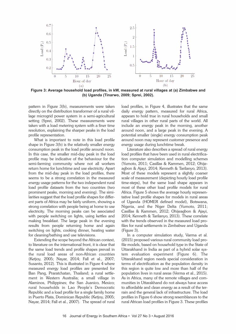
pattern in Figure 3(b), measurements were takendirectly on the distribution transformer of a rural vil-lage microgrid power system in a semi-agriculturalsetting (Sprei, 2002). These measurements weretaken with a load metering system with a finer timeresolution, explaining the sharper peaks in the loadprofile representation.
What is important to note in this load profileshape in Figure 3(b) is the relatively smaller energyconsumption peak in the load profile around noon.In this case, the smaller mid-day peak in the loadprofile may be indicative of the behaviour for thesemi-farming community where not all workersreturn home for lunchtime and use electricity. Apartfrom the mid-day peak in the load profiles, thereseems to be a strong correlation in the measuredenergy usage patterns for the two independent ruralload profile datasets from the two countries (twoprominent peaks, morning and evening). The simi-larities suggest that the load profile shapes for differ-ent parts of Africa may be fairly uniform, showing astrong correlation with people being at home to useelectricity. The morning peaks can be associatedwith people switching on lights, using kettles andmaking breakfast. The large peak in the eveningresults from people returning home and againswitching on lights, cooking dinner, heating waterfor cleaning/bathing and use televisions.
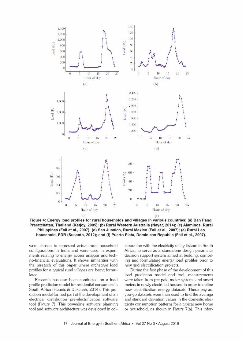
Extending the scope beyond the African context,to literature on the international front, it is clear thatthe same load trends and profile shapes prevail inthe rural load areas of non-African countries(Ketjoy, 2005; Nayar, 2014; Fall et al., 2007;Susanto, 2012). This is illustrated in Figure 4 wheremeasured energy load profiles are presented forBan Pang, Praratchatan, Thailand; a rural settle-ment in Western Australia; a small village inAlaminos, Philippines; the San Juanico, Mexico;rural households in Lao People’s DemocraticRepublic and a load profile for a single family homein Puerto Plata, Dominican Republic (Ketjoy, 2005;Nayar, 2014; Fall et al., 2007). The spread of rural
load profiles, in Figure 4, illustrates that the samedaily energy pattern, measured for rural Africa,appears to hold true in rural households and smallrural villages in other rural parts of the world. Allinclude an energy peak in the morning, anotheraround noon, and a large peak in the evening. Apotential smaller (single) energy consumption peakaround noon may represent customer presence andenergy usage during lunchtime break.
Literature also describes a spread of rural energyload profiles that have been used in rural electrifica-tion computer simulation and modelling schemes(Yumoto, 2011; Casillas & Kammen, 2012; Ohije-agbon & Ajayi, 2014; Kenneth & Tarilanyo, 2013).Most of these models represent a slightly coarserscale of measurement (depicting hourly load profiletime-steps), but the same load shape appears inmost of these other load profile models for ruralAfrica. Figure 5 shows the average hourly represen-tative load profile shapes for models in rural areasof Uganda (HOMER defined model), Botswana,Nigeria, and the Niger Delta (Yumoto, 2011;Casillas & Kammen, 2012; Ohijeagbon & Ajayi,2014; Kenneth & Tarilanyo, 2013). These correlatewith the trends observed in the measured load pro-files for rural settlements in Zimbabwe and Uganda(Figure 3).
In a computer simulation study, Varma et al.(2015) proposed various rural community load pro-file models, based on household type in the State ofUttarakhand in India as part of a hybrid solar sys-tem evaluation experiment (Figure 6). TheUttarakhand region needs special consideration interms of electrification as the population density inthis region is quite low and more than half of thepopulation lives in rural areas (Verma et al., 2015).As in Africa, many of the remote villages and com-munities in Uttarakhand do not always have accessto affordable and clean energy as a result of the ter-rain and the general lack of infrastructure. The loadprofiles in Figure 6 show strong resemblances to therural African load profiles in Figure 3. These profiles
16 Journal of Energy in Southern Africa • Vol 27 No 3 • August 2016
Figure 3: Average household load profiles, in kW, measured at rural villages at (a) Zimbabwe and(b) Uganda (Tinarwo, 2009; Sprei, 2002).
were chosen to represent actual rural householdconfigurations in India and were used in experi-ments relating to energy access analysis and tech-no-financial evaluations. It shows similarities withthe research of this paper where archetype loadprofiles for a typical rural villages are being formu-lated.
Research has also been conducted on a loadprofile prediction model for residential consumers inSouth Africa (Heunis & Dekenah, 2014). This pre-diction model formed part of the development of anelectrical distribution pre-electrification softwaretool (Figure 7). This powerline software planningtool and software architecture was developed in col-
laboration with the electricity utility Eskom in SouthAfrica, to serve as a standalone design parameterdecision support system aimed at building, compil-ing and formulating energy load profiles prior tonew grid electrification projects.
During the first phase of the development of thisload prediction model and tool, measurementswere taken from pre-paid meter systems and smartmeters in newly electrified houses, in order to definenew electrification energy datasets. These pay-as-you-go datasets were then used to find the averageand standard deviation values in the domestic elec-tricity consumption patterns for a typical new homeor household, as shown in Figure 7(a). This infor-
17 Journal of Energy in Southern Africa • Vol 27 No 3 • August 2016
Figure 4: Energy load profiles for rural households and villages in various countries: (a) Ban Pang,Praratchatan, Thailand (Ketjoy, 2005); (b) Rural Western Australia (Nayar, 2014); (c) Alaminos, Rural
Philippines (Fall et al., 2007); (d) San Juanico, Rural Mexico (Fall et al., 2007); (e) Rural Laohousehold, PDR (Susanto, 2012); and (f) Puerto Plata, Dominican Republic (Fall et al., 2007).

18 Journal of Energy in Southern Africa • Vol 27 No 3 • August 2016
Figure 5: Computer models for selected daily rural energy load profiles for various Africancountries (a) Homer model, rural Africa (Casillas & Kammen, 2012); (b) Botswana (Yumoto, 2011);(c) Sokoto, North-west Nigeria (Ohijeagbon & Ajayi, 2014); and (d) Akassa, Niger Delta (Kenneth &
Tarilanyo, 2013).
Figure 6: Daily average connected load for rural village scenarios in India. (a) Small village 5–6small households; (b) Medium households, range of appliances; (c) Small standalone household;
and (d) Small standalone off-grid rural household (Verma et al., 2015).

mation was subsequently used in a predictionmodel and grid-planning strategy to compute prob-able domestic load curves for a group of newhouseholds, as shown in Figure 7(b). This predic-tion model and tool was developed to help antici-pate consumption levels in newly planned electricalgrids as well as in planning distribution retrofits forgrid power network infrastructure extensions to newvillage zones and small towns.
By nature of the demand side load modellingtechnique, the load characteristics and electricityconsumption patterns in Figure 7 represent profilesfor newly planned homes in grid-connected town-ship areas, where newly built homes are often fittedwith electrical water heaters. These, and the addi-tion of other appliances that would not typically bepresent in off-grid households, may explain themid-day variations in the daily energy consumptionprofiles when comparing urban housing load pro-files to the load profile shapes for rural villagehomes as shown earlier in Figure 3.
3.2 Rural thermal energy profile shapesThe consumption load profiles for thermal energy,like electrical energy, are also presented on a two-dimensional chart that shows the instantaneousthermal or electrical load in kilowatts over 24 hours.This again offers a convenient way to visualise geo-metrical profiles for thermal energy usage patternsand to observe dynamic timing variations in thethermal load requirements, while making it easy tostudy the temporal load variations and changes.Since the current research focus is on water-cooledmicro-CHP systems, the interest in thermal energyin this paper is largely biased toward rural hot waterusage. In an electrified rural environment, hot waterusage makes up, on average, 30–50% of total ener-gy usage (Harris et al., 2008).
As with the electrical energy profiling exercise, itwas found that very little data was available on hotwater usage in rural African village settlements.Electronic datasets on hot water draw-off patternsfor off-grid isolated rural areas are virtually non-
19 Journal of Energy in Southern Africa • Vol 27 No 3 • August 2016
Figure 7: Load prediction with a grid distribution pre-electrification tool. (a) Average and standarddeviation profiles; (b) Predicted energy profile and deviation (Heunis & Dekenah, 2014).
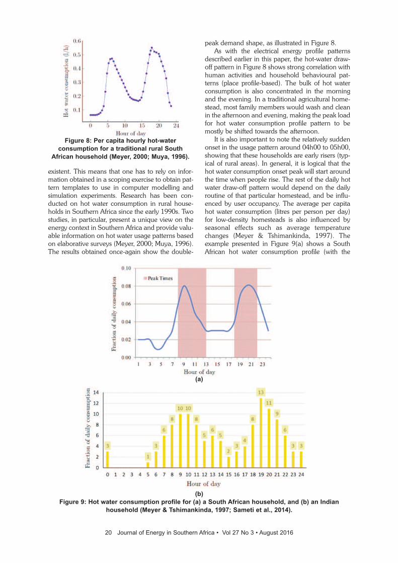
existent. This means that one has to rely on infor-mation obtained in a scoping exercise to obtain pat-tern templates to use in computer modelling andsimulation experiments. Research has been con-ducted on hot water consumption in rural house-holds in Southern Africa since the early 1990s. Twostudies, in particular, present a unique view on theenergy context in Southern Africa and provide valu-able information on hot water usage patterns basedon elaborative surveys (Meyer, 2000; Muya, 1996).The results obtained once-again show the double-
peak demand shape, as illustrated in Figure 8.As with the electrical energy profile patterns
described earlier in this paper, the hot-water draw-off pattern in Figure 8 shows strong correlation withhuman activities and household behavioural pat-terns (place profile-based). The bulk of hot waterconsumption is also concentrated in the morningand the evening. In a traditional agricultural home-stead, most family members would wash and cleanin the afternoon and evening, making the peak loadfor hot water consumption profile pattern to bemostly be shifted towards the afternoon.
It is also important to note the relatively suddenonset in the usage pattern around 04h00 to 05h00,showing that these households are early risers (typ-ical of rural areas). In general, it is logical that thehot water consumption onset peak will start aroundthe time when people rise. The rest of the daily hotwater draw-off pattern would depend on the dailyroutine of that particular homestead, and be influ-enced by user occupancy. The average per capitahot water consumption (litres per person per day)for low-density homesteads is also influenced byseasonal effects such as average temperaturechanges (Meyer & Tshimankinda, 1997). Theexample presented in Figure 9(a) shows a SouthAfrican hot water consumption profile (with the
20 Journal of Energy in Southern Africa • Vol 27 No 3 • August 2016
Figure 8: Per capita hourly hot-waterconsumption for a traditional rural South
African household (Meyer, 2000; Muya, 1996).
(b)Figure 9: Hot water consumption profile for (a) a South African household, and (b) an Indian
household (Meyer & Tshimankinda, 1997; Sameti et al., 2014).
(a)

peak band marked in the maroon bars), and Figure9(b) shows a so-called Rand profile for the fractionof daily hot water energy consumption. This Randprofile is an archetypal profile pattern profile shapeused to represent daily hot water consumption (120litres at a temperature of 50 °C) for a family of four(Sameti et al., 2014). These profiles agree with thefindings of Meyer shown in Figure 9.
The REEE 5/99 report on the Simulation andmonitoring of solar powered electric water heatingsystems in Namibia used pre-installed digital datalogging and flow rate recording equipment to reporton hot water usage patterns in rural Namibia(EMCON, 2000). The report shows graphs of hotwater consumption patterns measured at sites inNamibia, with plots of hot water draw-off patternsin terms of month-days, week-days and daily-hoursmeasured in a variety of households. Figure 10shows the hot water drawing pattern for an inde-pendently located low-income household of sevenpeople (EMCON, 2000). The data was recordedwith a digital data logger to show two importantresults. Figure 10(a) shows the household’s typicalhot water consumption for each day of the week,and Figure 10(b) shows the average hourly hotwater consumption profile for the household inhour time steps.
This section concludes with a reference to thethermal energy requirements related to cooking in arural African village. The micro-CHP system will beable to supplement some of the heat required for
cooking, which is why this thermal energy profile isconsidered to be important. In this regard, Figure11 shows a digitised version of a daily cooking pro-file, indicating the electricity used for a recently elec-trified rural homestead in southern Africa (Crossand Gaunt, 2003).
Although this paper will not discuss this profile indetail, it is valuable to note that the cooking profileis similar to the hot water usage profile. Once again,occupant behaviour may be related to the profilepeaks and will vary between households. From theinformation presented in this part of the scopingexercise, one can more confidently define appropri-ate load requirements for rural African communi-ties. The above exercise thus forms the basis for for-mulating a reference daily energy profile, in antici-pation of a potential transition for the villagetowards a modern solar co-generation supply sys-tem.
4. Consolidation of the load profiling resultsLoad profiling and energy consumption analysis iscentral in energy usage planning and micro-CHPmodelling analysis for isolated and remote ruralareas. Realistic load profiles are required, and serveas a guideline for the supply system design, as wellas the dynamic distribution viability on the demandside. This scoping exercise focused on the thermal(mainly hot water) and electrical load profiles. Theresults should be presented in a data format suitablefor reading or import by thermodynamic and elec-trical multi-carrier microgrid technology platformsand smartgrid software simulation platforms. Thesecomputer modelling simulation tools typically usethe terms ‘Rows-per-day’ or ‘Single-column data’ todescribe the format used to save data. In the Rows-per-day format, daily load profile data is saved as24-hour packets (i.e. date, time, kWh) in a singlerow with the following day in the next row, etc. Inthe single column format, all the data can be savedin a single column. In these formats, every linerecord in the dataset may contain several energy
21 Journal of Energy in Southern Africa • Vol 27 No 3 • August 2016
(b)Figure 10: Recorded hot water draw-offpatterns for a low-income homestead in
Namibia, showing the average hot water draw-off pattern per week (a) and draw-off per day (b)
(EMCON, 2000).
Figure 11: Daily cooking activity profile for ruralhouse in South Africa (Cross & Gaunt, 2003).
(a)

parameter fields, separated by a comma, semi-colon, tab or blank characters.
The focus of this study is on finding load profileshapes for hot water and electricity consumptionthat are typical for rural African households. Thismeans that less emphasis is placed on the actualquantity of energy used (kW or litres of hot water),but rather on the amount used per time step relativeto other times of the day. The aim is to provide ascientific base for evaluating and comparing tech-nology options and control automation optionsbased on realistic load profile patterns for Africanvillages. At the same time, an understanding isrequired of the operational requirements in an off-grid village with no previous access to electricity.This will assist in emulating a profile that is realisti-cally comparable to experiences and trendsobserved in the load patterns from recently electri-fied rural homes. This, in turn, can be used in com-puter models and simulation experiments aimed atrural African customised system design. The previ-ous section described the context and circum-stances around rural African village energy con-sumption. Following an energy load profile scopingexercise, the background from available literatureallows one to experiment with realistic thermalpower consumption patterns in such locations(Tinarwo, 2008; Sprei, 2002; Meyer, 2000; Muya,1996). The remainder of the discussion offers basicarchetypal energy reference shapes for rural heatand power load profiles aimed at micro-CHPresearch for rural Africa.
4.1 Rural African village electricity useprofile pattern: ScopingFrom the scoping exercise, a load profile thatdefines a realistic reference consumption pattern fora rural African homestead needs to be selected. Thekey aspect in defining the archetype is the one thatrelates to the time of energy consumption over a 24hour time interval.
In this paper, Section 2 presented informationon the patterns of rural African electricity usage,with data and plots offering various options fromwhich to select a potential candidate load profilereference pattern for use as electrical load patternfor remote isolated rural village homesteads inAfrica. The shape of the electrical load profile forrural Western Australia (Figure 4(b)) may seem par-ticularly familiar, as it has informally become a stan-dard or benchmark reference in many studies thatrequire a rural energy load profile and is often usedas an exemplary load profile in computer modellingstudies (Ibrahim & Ilinca, 2012; Nayar, 2014). It issimilar to the profiles measured by Tinarwo (2008)in Figure 3(a) and Sprei (2002) in Figure 3(b),which are other attractive candidates, both correlat-ing well with the experimental energy load profilemodels developed as representative models of ener-
gy consumption in rural African (Casillas &Kammen, 2012; Yumoto, 2011; Ohijeagbon &Ajayi, 2014; Kenneth and Tarilanyo, 2013). Of allthe load profile shapes observed in this scopingexercise, the model in Figure 3(b) was found to beparticularly valuable. This profile represents therural African village context in a realistic way. Theshape also correlates fairly well with rural profiles inother developing countries (Figure 4), as well aswith African village load profile models generallyused in computer simulation models (Figure 5).Since the Sprei (2002) dataset was measured with ahigh time-resolution, the load data should besmoothed to be comparable to hour-based resolu-tion load profiles typically used in computer simula-tion models. For this reason, an interpolation algo-rithm was used on the measured dataset of Sprei toprovide smoother average hourly energy usagesamples. The resulting archetypal reference loadprofile is presented in Figure 12.
By using inverse algorithmic curve fitting tech-niques, one can further approximate this referencerural power load profile in terms of a mathematicalexpression. The formula given in Equation 1 offersone such approximation for the load Pe profiledepicted in Figure 12, representing the electricalpower consumption (kW) for a typical rural villagedemand load as a function of time.
Pe = e[sin(0.3409−sin(0.68039t)−0.16801t)] (1)
An important aspect in defining a referencearchetype energy profile for a rural African home-stead or village is to define the amplitude scale forthe hourly load curve. This scale may represent theaverage daily level of the energy consumption, orthe hourly power kW requirement for the house-hold or rural village. From a rural African referenceload profile perspective, one can correlate thisrequirement with government regulations, with IEAlocal load estimates, or alternatively to conduct aload synthesis analysis to determine the integratedscaled village load profile amplitudes (IEA, 2014,Prieto-Araujo et al., 2015).
From Table 3, it was noted that the monthlyenergy consumption level for a rural household notcooking with electricity is around 150 kWh, whilethe energy consumption for electricity cookinghouseholds averaged around 210 kWh per house-hold (Lloyd & Cowan, 2004). An average monthlyenergy consumption level of 150 kWh per monthper rural household equates to approximately0.484 kWh per household per day. This estimatedaverage daily electricity load would thus spread outover the 24-hour time period in accordance withthe proposed archetypal hourly rural load profileshape in Figure 12. This would give the correctamplitude scaling of the curve.
When the village size changes, load scaling must
22 Journal of Energy in Southern Africa • Vol 27 No 3 • August 2016

further be used. In this way one can vary load pro-file magnitude as a function of village size (numberof clustered homesteads grouped in a small rural vil-lage, connected to the same local microgrid distri-bution line). This means that the same geometricshape for the reference archetype energy profile inFigure 12 would be used to represent any villagesize by scaling the amplitude based on the numberof houses. Figure 13 offers the final proposed anddigitised hourly load time-series graph for a ruralvillage settlement suitable for microgrid controlintelligence analysis and experimentation. This digi-tised generic hourly scaled computer modellingdataset version of the proposed hourly rural villageenergy consumption profile is presented in anhourly format suitable for use in energy systemsanalysis and computer simulation platforms (i.e.TRNSYS, Homer, EnergyPlus, EnergyPlan, ReEds,REopt), as well as transactive financial and eco-
nomic analysis packages (i.e. SAM, CREST,Community Solar Scenario).
4.2 Rural African hot water profile pattern:ScopingIn terms of hot water consumption in a rural Africanenergisation context, micro-CHP computer simula-tion evaluation experiments further require infor-mation about hot water usage in a rural African vil-lage. A valuable option is to learn from solar hotwater draw-off patterns measured at flat-plate andevacuated tube solar hot water systems at remotelocations. In general, domestic hot water patternsare driven by water use for household activitiessuch as house cleaning, washing dishes, washinglaundry, bathing and cooking. At the same time,this domestic hot water typically needs to be heatedin a hot water heater and stored at around 55 °C,and then applied at a blended outlet temperature of
23 Journal of Energy in Southern Africa • Vol 27 No 3 • August 2016
Figure 12: Potential rural electrical energy load profile reference shape for micro-CHP computermodelling and simulation experimentation.
Figure 13: Reference hourly electrical energy load profile for rural African village suitable for micro-CHP computer modelling and simulation experimentation.

around 40–45 °C (Agama, 2002).In the case of the first Namibian low-income
household (Figure 10), seven people occupied thedwelling. The average measured daily hot waterconsumption per day was 14.4 ± 4.8 l/person,while a second low-income household with twoinhabitants showed an average daily consumptionof 23.7 ± 5.8 l/person (EMCON, 2000). The dailyhot water consumption of rural African villageswithout access to municipal water is typically lowerthan the numbers found in this study (Meyer,2000). While the exact amount of hot water used ineach case may be different, the usage pattern inboth of these studies follow the same trend.
Figure 8 shows the chosen geometric shape forhot water draw-off patterns which is based onextensive research by Muya (1996) and Meyer(2000) and should serve as the guideline in profile-based central domestic hot water distribution.Figure 14 represents the digitised computer mod-elling version of the proposed hourly hot waterdraw-off profile in a format suitable for use in com-puter software simulation and thermodynamic anal-ysis platforms. This hourly time series hot waterdraw-off profile dataset can also be used to helpvalidate and compare mathematical and computersimulation models for storage and control automa-tion solutions in micro-CHP models.
The above load profiling and energy/hot waterconsumption analysis is central in the energy usageplanning and micro-CHP modelling analysis for iso-lated and remote rural areas. The above sectionoffers realistic load profiles in format suitable forcomputer simulation platforms. These profiles cannow be used as archetype rural consumption refer-ence shapes in solar microgrids and solar micro-CHP system simulation experiments. It will in futurealso be helpful in comparing embedded off-grid dis-
tribution management system control schemes andstand-alone distributed energy resource manage-ment system approaches in micro-CHP microgridsimulation experiments.
5. ConclusionsA community solar micro-CHP system generates
energy from variable renewable energy sources. Insuch shared community energy systems, specialconsideration should be given to a control automa-tion and energy management solution. Such a solu-tion should be capable of energy conservation aswell as energy supply and demand-balancing inscalable community microgrid configurations. Todevelop and evaluate suitable computer-guidedcontrol automation and storage solutions for digitalmicro-CHP system models in isolated rural micro-grid applications, reference energy consumptionprofiles for the use (or potential use) of thermal andelectrical energy usage is required. Even with theavailability of Big Data and Smart metering, it is stillproving to be difficult to find thermal and electricalenergy profile shapes for a rural African village. Ascoping exercise was subsequently performed toinvestigate how literature data can be used asmeans to define universal load profile shapes for aremote and isolated rural African context (Cross &Gaunt, 2003; Heunis & Dekenah, 2014; Meyer,2000; Muya, 1996; OpenEI, 2015; Tinarwo, 2009;Sprei, 2002).
The results from the scoping exercise showedthat the thermal and electrical profiles for domesticrural energy had certain characteristic features. Themost important is the two peaks that have beenextensively discussed. The scoping exercise showedthat the peaks in the electrical and thermal loadscoincided with the patterns of user activity, beingpresent in the early morning and in the evening,with the latter always being more prominent. In
24 Journal of Energy in Southern Africa • Vol 27 No 3 • August 2016
Figure 14: Proposed characteristic rural domestic hot water profile archetype reference shape formicro-CHP computer modelling and simulation experimentation

some cases, a peak around noon could be seen andwas mostly associated with agricultural communi-ties.
From the scoping exercise, hot water usage byrural households is better understood. There ismuch more consistency in the data, which is differ-ent from electricity usage in rural households wherepatterns fluctuate greatly between studies. Thismeans that even though the time of electricity con-sumption is known, it is difficult to know how muchgeneration the system needs to be designed for. Thescoping profile can also serve as baseline load in thedevelopment of a software tool to formulate andpredict load profiles in multi-carrier microgrids foroff-grid rural areas.
The outcome of the scoping exercise offers digi-tised computer model ready hourly electricity andhourly hot water draw-off profiles in a format suit-able for use in dynamic microgrid analysis andcomputer software for energy simulation platforms(i.e. TrnSys, Homer Energy, EnergyPLAN,EnergyPlus, ReEds, RetScreen, Leap, andOSeMOSYS). These hourly time series electricityusage and hot water draw-off profile datasets cannow be used to help validate and compare mathe-matical and computer simulation models for storageand control automation solutions in micro-CHPmodels. It will also be useful in techno-economicanalyses for integrated or isolated district communi-ty energy systems. Disaggregated load profiles(radio, TV, cellphone charger, lights, security sys-tem) derived from the above load profiles will fur-ther help to develop demand response, demandmanagement, responsive load curtailment anddynamic load control systems, to account forrenewable supply variability in distributed energyresources within sustainable rural development sys-tems.
AcknowledgmentsThe authors thank the South African Department ofScience and Technology, the National ResearchFoundation for funding this research work.
ReferencesAfrica, L., Blore, M., Dwight, R., Reichhardt, C., Retief,
D., Mpando, T., 2008. Domestic energy use of lowincome households in Grahamstown East. State ofthe Environment Report (SoER) for Grahamstown,Eastern Cape, 1–29.
Agama, 2002. Sustainable Energy Services, LynedochEco-Village. AGAMA Energy (Pty) Ltd P O Box 606,Constantia, 7848, South Africa, 1–28.
Aron, J., Eberhard, A., Gandar, M., 1991. Fuelwooddeficits in rural South Africa. Biomass and Bioenergy1 (2); 89–98.
Barbieri, E. S., Spina, P. R., Venturini, M., 2012.Analysis of innovative micro-CHP systems to meet
household energy demands. Applied Energy 97:723–733.
Bokanga, G. M., Kahn, M. T. E., 2014. Design of a lowvoltage DC microgrid system for rural electrificationin South Africa 25 (2), 9–14.
Casillas, C. E., Kammen, D. M., 2012. The challenge ofmaking reliable carbon abatement estimates: Thecase of diesel microgrids. S.A.P.I.EN.S. Surveys andPerspectives Integrating Environment and SocietyJournal 5 (1).
Cho, H., Eksioglu, S. D., Luck, R., Chamra, L. M.,2008. Operation of a CCHP system using an opti-mal energy dispatch algorithm. ASME 2008 2ndInternational Conference on Energy Sustainabilitycollocated with the Heat Transfer, FluidsEngineering; 1–8.
Cho, H., Luck, R., Chamra, L. M., 2007. Dynamic simu-lation of a Micro-CHP facility: A case study. ASME2007 Energy Sustainability Conference, LongBeach, California, USA; 247–254.
Cross, N., and Gaunt, C., 2003. Application of rural res-idential hourly load curves in energy modelling.IEEE Conference: Power Tech ConferenceProceedings, 2003 IEEE Bologna; 1–4.
Dagbjartsson, G., Gaunt, C., Zomers, A., 2007. Ruralelectrification: A scoping report. Cigre WorkingGroup C6-13 Rural Electrification Workshop 1; 1–24.
Damte, A., Koch, S. F., Mekonnen, A., 2012. Copingwith Fuelwood Scarcity. Household Responses inRural Ethiopia. Environment for Development.Disucssion Paper Series 12-01 (January), 1–34.
Deloitte, 2011. Advanced metering infrastructure cus-tomer impacts study. Department of PrimaryIndustries, Victoria, Australia, Final report: Volume 1and 2 (1), 1–89.
Department of Minerals and Energy, 2003. Electricitybasic support services tariff (Free basic electricity)policy. Pretoria: Department of Minerals and Energy,South Africa (DME), 1-5.
EMCON, 2000. Simulation and monitoring of solar andelectric water heating systems. REEE 5/99, EMCONConsulting Engineers for Ministry of Mines andEnergy Private Bag 13297, Windhoek, Namibia, 1–116.
Fall, N., Giles, L., Marchionini, B., Skolnik, E. G., 2007.Remote area power supply (RAPS) load andresource profiles: A study for the DOE energy stor-age program. SAND REPORT SAND2007-4268Unlimited Release Printed July 2007 (July), 47.
Fogarty, A., 2015. African Kaleidoscope Safari, Code(OV08) A 12 day tour. Overnight Tours 1 (1), 1–2.[online]http://mobi.alantours.co.za/mobi_listings/overnight_tours (accessed 1 Sept 2015).
Harris, A., Kilfoil, M., Uken, E., 2008. Options for resi-dential hot water heating. Energy Technology Unit,Cape Peninsula University of Technology, CapeTown, South Africa, 1–8.
Heunis, S., Dekenah, M., 2014. A load profile predic-tion model for residential consumers in South Africa.Proceedings of the 22nd Conference on theDomestic Use of Energy, DUE 2014, 3–8.
25 Journal of Energy in Southern Africa • Vol 27 No 3 • August 2016
Ho, C. K., 2008. Software and codes for analysis of con-centrating solar power technologies. Sandia NationalLaboratories, Report SAND2008-8053 (December),1–35.
Hussein Ibrahim, H. and Ilinca, A., 2012. Contributionof the Compressed Air Energy Storage in theReduction of GHG - Case Study: Application on theRemote Area Power Supply System, Air Pollution - AComprehensive Perspective, Dr. Budi Haryanto(Ed.), InTech, DOI: 10.5772/50131.
International Energy Agency, 2014. Africa EnergyOutlook. A focus on the energy prospects in sub-Saharan Africa. World Energy Outlook SpecialReport, International Energy Agency Publication, 1–237.
iShack, 2013. The iShack: A business model for incre-mentally upgrading informal settlements.Sustainability Institute, Stellenbosch University(April), Stellenbosch, South Africa. 2011–2014.
Kenneth, A. P., Tarilanyo, A. J., 2013. Developing sus-tainable power supply for rural communities inAkassa of Bayelsa state using photovoltaic systemand battery. Research Journal of Applied Sciences,Engineering and Technology 6 (4), 545–550.
Ketjoy, N., 2005. Photovoltaic hybrid systems for ruralelectrification in the Mekong countries. University ofKessel, Library, 1–135.
Kruger, J. L., 2007. Towards an appropriate frameworkfor South African rural renewable energy provision.MPhil dissertation, Stellenbosch University,Stellenbosch, South Africa. (December), 1–180.
Lloyd, P., 2014. The energy profile of a low-incomeurban community. Domestic Use of EnergyConference, 29 March 2 April, 2014, Cape Town,South Africa 25 (3), 80–85.
Lloyd, P., Cowan, B., 2004. Improving access to electric-ity: Lessons from Khayelitsha. Energy ResearchCentre, University of Cape Town, South Africa, 1–6.
Lund, H., 2015. Renewable energy systems: A smartenergy systems approach to the choice and modelingof 100% renewable solutions. Academic Press, 225Wyman Street, Waltham, MA, USA, ISBN:9780124104235: 1-384.
Makungwa, S. D., Epulani, F., Woodhouse, I. H., 2013.Fuelwood supply: A missed essential component in afood security equation. Journal of Food Security 1(2); 49–51.
Masekoameng, K. E., 2005. Household energy needsand utilization patterns in the Giyani rural communi-ties of Limpopo Province, South Africa. Journal ofEnergy in Southern Africa 16 (3), 4–9.
Meyer, J. P., 2000. A review of domestic hot-water con-sumption in South Africa. R & D Journal 16; 55–61.
Meyer, J. P., Tshimankinda, M., 1997. Hot water con-sumption by developing communities in SouthAfrican traditional houses. International Journal ofEnergy Research 21 (12); 667–673.
Mulaudzi, S., Qase, N., 2008. New and renewable ener-gy: Mini-grid hybrid viability and replication poten-tial: The Hluleka and Lucingweni pilot projects.Department of Minerals and Energy of South Africa,1–299. Pretoria, South Africa.
Muya, T., 1996. Hot water consumption in South Africa.
Phd dissertation, Rand Afrikaans University (nowUniversity of Johannesburg), Johannesburg, SouthAfrica.
Nayar, C., 2014. Energy security in small islands andremote communities through innovative micro-gridsystems. Remote Area Power Supply Conference,Regen Power Sustainable Power Solutions (3), 1–65.
Ohijeagbon, O. D. and Ajayi, O. O., 2014. Potential andeconomic viability of standalone hybrid systems fora rural community of Sokoto, North-west Nigeria.Frontiers in Energy 8 (2); 145–159.
OpenEI, 2015. Commercial and residential hourly loadprofiles for all TMY3 locations in the United States.Available from http://en.openei.org/doe-opendata/dataset/commercial-and-residential-hourly-load-profiles-for-all-tmy3-locations-in-the-united-states [Accessed 25 Sept 2015].
Palmer, C., MacGregor, J., 2008. Fuelwood scarcity,energy substitution and rural livelihoods in Namibia.Proceedings of the German DevelopmentEconomics Conference, Zurich (32), 1–29.
Prieto-Araujo, E., Olivella-Rosell, P., Cheah-Mane, M.,Villafafila-Robles, R., Gomis-Bellmunt, O., 2015.Renewable energy emulation concepts for micro-grids. Renewable and Sustainable Energy Reviews,Elsevier 50; 325–345.
Prinsloo, G. J. and Dobson, R. T., 2015. Combinedsolar heat and power with microgrid storage and lay-ered smartgrid control toward supplying off-gridrural villages. Energy Science & Engineering 3 (2):135-144.
Reddy, Y., 2008. An exploration of household energyuse patterns among grid electrified households inlow-income rural and peri-urban communities inSouth Africa. PhD thesis, University of Cape Town,Cape Town, South Africa.
Sameti, M., Kasaeian, A., Mohammadi, S. S. andSharifi, N., 2014. Thermal performance analysis of afully mixed solar storage tank in a ZEB hot watersystem. Sustainable Energy 2 (2): 52–56.
Scheurlen, E., 2015. Time allocation to energy resourcecollection in rural Ethiopia gender-disaggregatedhousehold responses to changes in firewood avail-ability. IFPRI Discussion Paper 01419, Environmentand Production Technology Division, Internationalfood Policy Research Institute, 1–48.
Shackleton, C., Gambiza, J. and Jones, R., 2007.Household fuelwood use in small electrified towns ofthe Makana District, Eastern Cape, South Africa.Journal of Energy in Southern Africa 18 (3): 4–10.
Shilts, E. and Fischer, B., 2014. We plotted 812,000energy usage curves on top of each other, this is thepowerful insight we discovered. OPower Labs, Load-curve-archetypes. Available online:https://blog.opower.com/2014/10/load-curve-archetypes/ [Accessed 20 Sept 2015].
Sprei, F., 2002. Characterization of power system loadsin rural Uganda. Masters thesis, Lund University ofTechnology, Lund, Sweden.
Susanto, J., 2012. Limits of grid extension in the LaoPDR: A financial perspective. Journal ofHumanitarian Engineering 1 (1): 27–38.
Tinarwo, D., 2009. Design of village power and micro-
26 Journal of Energy in Southern Africa • Vol 27 No 3 • August 2016

grids for rural areas of Zimbabwe with specific atten-tion to voltage regulation on low voltage meshed dis-tribution grids. Kassel University Press, Kassel,Germany.
United Nations Development Programme, 2011.Sustainability and equity: A better future for all.Human Development Report, United NationsDevelopment Programme, New York. 1-58.
Verma, A., Biswas, S. and Ahmad, S. Y., 2015. Techno-financial analysis of energy access through hybridsystem with solar PV under the various rural com-munity models for State of Uttarakhand, India.Smart Grid and Renewable Energy 6 (April): 75–94.
World Health Organisation, 2010. Households usingsolid fuels as the primary cooking fuel, by WHOregion. WHO Global Health Observatory Repository,World Health Organisation, Geneva, Switzerland, 1–10.
Yumoto, N., 2011. Sustainability conditions for PVhybrid systems: Environmental considerations.Energy and Environment Institute, IEA PVPS Task11 Report IEA-PVPS T11-03:2011, 1–28.
27 Journal of Energy in Southern Africa • Vol 27 No 3 • August 2016

AbstractPartial shading of a PV module has received muchattention over the past few years, as it results inuneven cell power generation, compromising a PVsystem performance. Full uniform shading of a PVmodule has not received as much attention. Thisarticle correlates the percentage of full uniformshading of a given PV module within a controlledenvironment to its output power. The percentage offull uniform shading provided by shade nets wasfirstly determined. These shade nets are then usedto cover a specific PV module (experimental sys-tem), while an identical PV module remains totallyunshaded (control system). Increasing percentagesof full uniform shading negatively affected the directbeam component in a linear way. Decreasing thelight intensity falling on the PV model exhibited alinear increase in the percentage of output powerreduction of the PV module. This is observed in thata shade net providing 36% of full uniform shadingresulted in a 56% output power reduction, while a63% full uniform shading net yielded 82% powerreduction. These results hold a strong promise toimprove current simulation modules that focus ondetermining the output power of a given PV arrayunder specific environmental conditions or for spe-cialised geographical locations.
Keywords: partial shading, PV simulation, shadenet
Highlights1. Six different shade nets were quantified using
the shading experiment.2. A 36% shade net resulted in a 56% output
power reduction.3. A 63% shade net yielded 82% power reduction.
28
Journal of Energy in Southern Africa 27(3): 28–38
Varying percentages of full uniform shading of a PV module in a controlled environment yields linearpower reduction
Arthur James Swart, Pierre E. Hertzog*
Department of Electrical, Electronics and Computer Engineering, Central University of Technology, Private Bag X20539, Bloemfontein, 9300
Corresponding author: Tel.: +27 (0)51 507 3682 Email: [email protected]

1. Introduction‘Almost every way we make electricity today, exceptfor the emerging renewables and nuclear, puts outcarbon dioxide. And so, what we’re going to haveto do at a global scale is create a new system. Andso, we need energy miracles’ [1]. Energy miracles,as referred to by Bill Gates, require on-goingresearch into developing and understanding newenergy systems, including renewable energy sys-tems in the form of photovoltaic (PV) systems [2].The PV systems still require much research anddevelopment in order to improve efficiency andreduce manufacturing costs. In fact literature statesthat an ever-increasing need to improve the efficien-cy of energy production still exists today [3], espe-cially in view of the ever increasing global demand,as shown in Figure 1. This demand has a potentialto not only necessitate the production of more ener-gy (an increase of 60% by 2030), but also theincrease of carbon dioxide by an even greater per-centage (an increase of 62% by 2030).
The efficiency of PV cells varies depending onthe technology, light spectrum, atmospheric condi-tions, temperature, design and material used, andcan be up to 46% efficient [5]. The conventionalsolar PV panels have a conversion efficiency of only5–17% [6]. Interrupting direct beam radiation low-ers the output voltage of a PV module significantly,influencing the amount of output power availablefor driving an alternative energy system, which maylead to system downtime or even component failureover a period of time [7]. This interruption is usuallydue to cloud movement or shading of the PV mod-ule by natural or man-made causes. Partial shading
of a PV module has received much attention overthe past few years, as it results in uneven cell powergeneration that my compromise total power pro-duction [8]. Numerous simulation models were pro-posed to study the effect of partial shading, includ-ing the model by Tian et al. [9]. A Google ScholarSearch of the terms ‘partial shading’ and ‘photo-voltaic’ revealed some 3510 hits in December2014, while the words ‘uniform shading’ and ‘pho-tovoltaic’ revealed only 95 hits in that same month.
It must therefore be noted that research relatingto the exact effect that varying percentages of fulluniform shading exert on the output power of a PVmodule is lacking. For example, Giaffreda et al. [10]contrasted full uniform shading to partial shading ofa PV cell and proved that its cell temperaturesincreased when shaded. No percentages of varyingshade were, however, reported, nor the effect onthe output power. Results given by Christy regard-ing shading suggested that the reduction in currentwas not proportional to the amount of shading onthe PV panel [11]. Again, no varying percentages offull uniform shading were reported. Gummeson etal. [12] reported that a fully-shaded 11.4 cm2 PVmodule produced 29 times less power than thesame PV module under bright indoor lighting con-ditions. Again, no percentages of full shade werementioned, although a significant power reductionwas given. Johnson [13] used Blue Hawk 4 mmthick, heavy-duty plastic sheeting to cover the top ofPV modules to provide varying levels of insolation,which included unshaded, partially shaded andfully shaded modules. Power reduction was foundto be around 33% for full uniform shading. Again,
29 Journal of Energy in Southern Africa • Vol 27 No 3 • August 2016
Figure 1: Global energy demand [4].
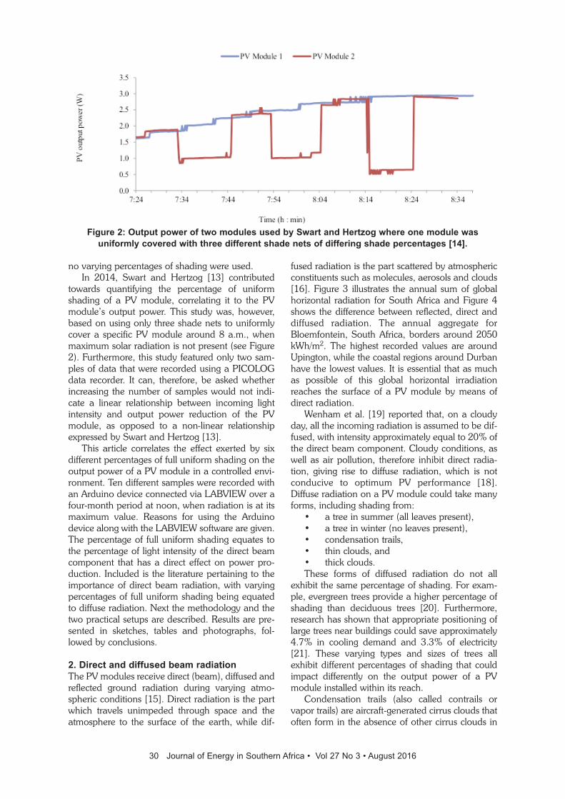
no varying percentages of shading were used. In 2014, Swart and Hertzog [13] contributed
towards quantifying the percentage of uniformshading of a PV module, correlating it to the PVmodule’s output power. This study was, however,based on using only three shade nets to uniformlycover a specific PV module around 8 a.m., whenmaximum solar radiation is not present (see Figure2). Furthermore, this study featured only two sam-ples of data that were recorded using a PICOLOGdata recorder. It can, therefore, be asked whetherincreasing the number of samples would not indi-cate a linear relationship between incoming lightintensity and output power reduction of the PVmodule, as opposed to a non-linear relationshipexpressed by Swart and Hertzog [13].
This article correlates the effect exerted by sixdifferent percentages of full uniform shading on theoutput power of a PV module in a controlled envi-ronment. Ten different samples were recorded withan Arduino device connected via LABVIEW over afour-month period at noon, when radiation is at itsmaximum value. Reasons for using the Arduinodevice along with the LABVIEW software are given.The percentage of full uniform shading equates tothe percentage of light intensity of the direct beamcomponent that has a direct effect on power pro-duction. Included is the literature pertaining to theimportance of direct beam radiation, with varyingpercentages of full uniform shading being equatedto diffuse radiation. Next the methodology and thetwo practical setups are described. Results are pre-sented in sketches, tables and photographs, fol-lowed by conclusions.
2. Direct and diffused beam radiationThe PV modules receive direct (beam), diffused andreflected ground radiation during varying atmo-spheric conditions [15]. Direct radiation is the partwhich travels unimpeded through space and theatmosphere to the surface of the earth, while dif-
fused radiation is the part scattered by atmosphericconstituents such as molecules, aerosols and clouds[16]. Figure 3 illustrates the annual sum of globalhorizontal radiation for South Africa and Figure 4shows the difference between reflected, direct anddiffused radiation. The annual aggregate forBloemfontein, South Africa, borders around 2050kWh/m2. The highest recorded values are aroundUpington, while the coastal regions around Durbanhave the lowest values. It is essential that as muchas possible of this global horizontal irradiationreaches the surface of a PV module by means ofdirect radiation.
Wenham et al. [19] reported that, on a cloudyday, all the incoming radiation is assumed to be dif-fused, with intensity approximately equal to 20% ofthe direct beam component. Cloudy conditions, aswell as air pollution, therefore inhibit direct radia-tion, giving rise to diffuse radiation, which is notconducive to optimum PV performance [18].Diffuse radiation on a PV module could take manyforms, including shading from:
• a tree in summer (all leaves present),• a tree in winter (no leaves present),• condensation trails,• thin clouds, and• thick clouds. These forms of diffused radiation do not all
exhibit the same percentage of shading. For exam-ple, evergreen trees provide a higher percentage ofshading than deciduous trees [20]. Furthermore,research has shown that appropriate positioning oflarge trees near buildings could save approximately4.7% in cooling demand and 3.3% of electricity[21]. These varying types and sizes of trees allexhibit different percentages of shading that couldimpact differently on the output power of a PVmodule installed within its reach.
Condensation trails (also called contrails orvapor trails) are aircraft-generated cirrus clouds thatoften form in the absence of other cirrus clouds in
30 Journal of Energy in Southern Africa • Vol 27 No 3 • August 2016
Figure 2: Output power of two modules used by Swart and Hertzog where one module wasuniformly covered with three different shade nets of differing shade percentages [14].

ice-supersaturated conditions at temperatures lessthan -39 °C [22]. Since such conditions are relative-ly common in the upper troposphere, contrails candevelop into relatively long-lived cirrus cloud [23].They can add to naturally occurring cloud coverand may be important for the earth’s radiative bal-ance [24]. Persistent contrails are an important cli-mate impact of aviation that could potentially bereduced by re-routing aircraft. This, however, gen-erally increases both the flight length and its corre-
sponding CO emissions [25]. Contrails are visiblefor several minutes, or even longer when the rela-tive humidity is slightly below saturation, in particu-lar at low temperatures [26]. A national flight oper-ator in South Africa has a number of scheduledflights between Johannesburg and Port Elizabeth,with the flight path often being directly overBloemfontein [27]. This results in a number of con-trails that are visible on the ground, especially dur-ing the colder winter months. However, these con-
31 Journal of Energy in Southern Africa • Vol 27 No 3 • August 2016
Figure 3: Daily average solar radiation for South Africa [17].
Figure 4: Different radiation beams [18].

trails may be considered to be cirrus-clouds that areusually optically thin in the sub millimeter [28], asshown in Figure 5.
Figure 5: Contrails are considered to be cirrusclouds which may be equated to thin clouds
[29].
Figure 5 shows that thin clouds are relativelytransparent to sunlight [30], thereby providing alower percentage of shading on the earth’s surfacewhen compared to thick clouds. These thin cloudsare hard to identify on satellite images because theyeither reflect too little solar radiation or block too lit-tle terrestrial emission [31], while thick clouds areeasier to detect [32]. Thick clouds are easy to distin-guish because they are obviously brighter, and usu-ally gathered together, forming a large block [33],resulting in a larger percentage of shading on theearth’s surface. PV modules, being exposed to boththin and thick clouds, are subjected to varying per-centages of shading [34].
These varying percentages of shading have thepotential to negatively influence PV-based systems,such as PV/hydro hybrid renewable energy systemsor innovative solar vehicles. In turn, these hybridgenerators could be used as a standby powersource for remote sites [35] where an importantrequirement would be the availability of directbeam radiation. In terms of solar vehicles, the sizeof the PV system is usually determined according tothe power and voltage requirements of the electricalmotor [36]. Direct beam radiation, as opposed todiffuse beam radiation, makes up the majority oftotal solar radiation and is required for the optimaloperation of these types of energy generator sys-tems and vehicles [37]. Quantifying the percentageof full uniform shading of a given PV module to itsoutput power may assist in optimising the designand development of these types of hybrid genera-tors and solar vehicles for varying percentages ofdirect beam radiation.
3. The PV technologyA typical PV cell generates around 0.6 V, dependingon the type of semiconductor used and the manu-
facturing technology employed [38]. To increasethe voltage and current requires several cells to beconnected in series and/or parallel to form a PVmodule. The working principle of a PV cell is basedon the ‘photovoltaic effect’ in that when sunlightfalls on a cell that consists of a normal p-n junction,photons are absorbed, resulting in electron-holepairs being generated [39]. Essentially, circuits thatcontain semiconductor devices are non-linear, mostobviously for devices such as diodes and silicon-controlled rectifiers where the IV characteristicschange abruptly [40]. The characteristics of PV cellsare therefore non-linear, depending to a largedegree on environmental parameters like tempera-ture, solar irradiation, shading, humidity and pres-sure [41]. It may, therefore, be hypothesised thatthe relationship between the incoming light intensi-ty and the output power of a PV module is non-lin-ear. One aim of this research is to either support orreject this hypothesis.
4. Research methodologyThe first objective of this study is to quantify thepercentage of the direct beam radiation that passesthrough the six different shade nets that will be usedin the full uniform shading of the PV modules. Thiswas done using two methods. In the first method, aconstant light source, light sensor and two blackcylinders (see Section 5 for setup) were used.Multiple tests done on the same day results in ahigher reliability coefficient than does a test–reteston separate days [42]. A number of tests were,therefore, done on the same day, using both ananalogue light intensity meter (PHYWE) and a dig-ital light intensity meter (ISO-TECH). This was doneto verify the percentages of light reduction that werestated by the manufacturers of the shade nets. Asecond method involved placing the shade netsdirectly over the sensor (placed at the same tiltangle as are the PV modules) of the light intensitymeter, using the sun as the light source.
The second study objective is to correlate thedifferent percentages of full uniform shading to theoutput power of a PV module (termed PV Module2). Each shade net was used to cover PV Module 2for one minute (experimental system), with one-minute intervals where no shading was used. Thisenabled PV Module 2 to return to normal operationin line with PV module 1, which remained com-pletely unshaded (control system) for the durationof the tests. Multiple samples were acquired on dif-ferent days of the months (May–August 2014)around 11:30 am, as maximum solar radiationoccurred around noon. The reasons for using thistime period was the low rainfall during thesemonths at the research site.
The multiple samples within a natural settingensured reliability and validity of the results. Thereliability of a study begins to decrease when it
32 Journal of Energy in Southern Africa • Vol 27 No 3 • August 2016

becomes more difficult to replicate the results [43],and would therefore be increased if the same resultswere obtained over a period of time.
5. Practical setup 1: Determining shadingpercentagesA constant light source, light sensor and cylinderswere used in order to establish an environment withminimum influence from external light. Two blackcylinders (each 525 cm long and 27 cm in diame-ter) were staked upon each other (see Figure 6).The top cylinder was sealed from external light anda 12 V, 3 W (230 lm) light-emitting diode (LED)lamp was securely mounted in the centre of the topcylinder as a light source. In the control system, theLED lamp was switched on and the light intensitymeasured using an analogue PHYWE light intensitymeter (light sensor mounted at the bottom of thebottom cylinder) and a digital ISO-TECH lightintensity meter. Six different percentages of shadenet were placed between the top and bottom cylin-ders (525 cm from the light source and light sensor)in the first method. In this instance, light from thelight source would have to travel through the shadenet to reach the light sensor. This light intensity wasmeasured to enable the exact calculations of theshading percentages. These shade nets were thenused in the practical setup of the PV system. In thesecond method, the sensors of the light meters wereplaced at the same tilt angle of the PV modules. Theshade nets were then placed directly over the sen-sors, just as the shade nets would be placed directlyover the surface of the PV modules. Three differentsamples were obtained from which the averagesvalues were used.
Figure 6: Practical setup for verifying the shadenet specifications.
6. Practical setup 2: Identical PV systemsNo batteries were included in the practical setup ofthe two identical PV systems because of uncertain
variations that might exist between batteries fromthe same manufacturer and with the same modelnumber. In fact, battery-to-battery variations inelectromotive force at a given state of charge couldbe in the order of 50 mV due to variations in themanufacturing process, ageing and charge-dis-charge cycling of a single 2.25 V cell [44]. A 60 LEDlamp (12 V, 3 W) was, therefore, chosen as the loadresistance that was connected directly to the PVmodule via a 22 Ω resistor. The purpose of theseries resistor was to raise the threshold operatingvoltage and ensure that the voltage across the LEDnever exceeded 12 V, as the stated output voltage ofthe PV module used was 16.5 V at standard testconditions. The threshold operating voltage is thepoint at which the LED starts emitting light, despitebeing very faint. A data logging interface wasincluded between the PV module and the LEDlamp, which served to condition the voltage andcurrent from the PV module to enable logging viaan ARDUINO board to a PC. This circuit was basedon Swart [45] and Asowata [46, 47].
The ARDUINO board is an electronic platformdesigned to simplify the process of studying digitalelectronics, and comprises a microcontroller, a pro-gramming language and an integrated develop-ment environment [48]. The ARDUINO was estab-lished to teach interaction design, a design disci-pline that puts prototyping at the centre of itsmethodology [49]. The hardware is relatively cheapand the development software can be downloadedfor free from the internet. There are also a growingnumber of freely-available software examples thatmake the implementation of ideas on these boardseasier to achieve. Academics from different fieldsmake extensive use of these ARDUINO boards [50-52]. These boards are used in conjunction with theNational Instruments LabVIEW software, a graphi-cal programming language that has its roots inautomation control and data acquisition [53]. TheLabVIEW has several key features that make it agood choice in an automation environment andincludes simple network communication, turnkeyimplementation of common communication proto-cols, powerful toolsets for process control and datafitting, fast and easy user interface construction, andan efficient code execution environment [54]. Thepractical setup is shown in Figure 7. Six differentshade nets (with exact measured and calculatedshading percentages) were placed over PV Module2 (becoming the experimental system – Point A inFigure 7), while PV Module 1 remained completelyunshaded (becoming the reference or control sys-tem – Point B in Figure 7). An aluminum frame,with a protractor placed 90º due North, was con-structed to securely mount the two identical 10 WPV modules (Point D in Figure 7). This protractorwas used to verify the direct alignment of the sun tothe PV modules at 12:00. The modules were
33 Journal of Energy in Southern Africa • Vol 27 No 3 • August 2016

mounted at the same tilt angle of 39º, equating tothe latitude value of 29º plus 10º for the CentralUniversity of Technology, Bloemfontein. Values oflatitude plus 10º for PV module tilt angles in SouthAfrica were suggested by Chinnery [55] and sub-stantiated by Asowata [56]. The practical setup wasdone inside an air-conditioned room where thetemperature was kept constant at 24 . This was inorder to prevent excess temperature degradationthat has a significant effect on the output voltage ofa PV module [57]. Due to the low output power ofthese PV modules as well as the short period of time(one minute) in which the shading nets wereapplied, no significant temperature differencesbetween the two modules were observed. The cur-rent through the LED lamp (Point C in Figure 7indicating that Module 1 is completely unshaded) aswell as the voltage across it was logged for both thecontrol and the experimental system.
Figure 7: Practical setup of the two identical PVsystems. Points A = the experimental system, B
= control system, C = LED lamp, D = twoidentical 10 W PV modules.
These voltage and current values (for both theexperimental and control system) were then used tocalculate the output power of the PV module, withthe percentage of power reduction being calculatedusing Equation 1. The aluminum frame was placedagainst a north-facing large glass window (Point Cin Figure 8). Point A represents Module 2 (experi-mental system) and Point B represents Module 1(control system) in Figure 8.
% Power reduction= 100 (1)
7. Results and discussionThe results of the shading experiment are shown inFigure 9. Using both the noon SUN and two differ-ent LEDs (3 W and 4 W) revealed similar resultsusing the different shade nets that were sandwichedbetween two black pipes, according to Figure 6.The 22% shade net (Net 1) allowed 80% of light topass, while a 42% shade net (Net 3) allowed 60%of light to pass. A 92% shade net (Net 6) onlyallowed 10% of light to pass. This, consequently,yielded a negative linear relationship (R2 = 0.9807)between shade net percentage increase and light
intensity decrease. The results for the 3 W LED, 4W LED and the SUN-2Pipes were recorded usingthe first method described in Section 5 in relation toFigure 6. The second method, using only the sunand shade nets placed directly over the tilted sensorof the light meters (thereby replicating the setup ofthe shade nets and PV modules), provided theresults given for the SUN experimental setup shownin Figure 9.
Figure 10 shows the power reduction for a PVmodule (PV Module 2 represented by the yellowline), which was exposed to six shade nets with dif-ferent shading percentages. This sketch is obtainedfrom the LabVIEW interface that was developed forthis investigation. The sampling interval was set atone second and the different shade nets were usedin one-minute intervals in order to give the systeman opportunity to stabilise after each given event.The PV Module 1 (red line) exhibited a continuousoutput power and served as a control experiment.Figure 10 shows evidence of power reduction foreach increase in shade net percentage. This trendwas reversed as smaller percentages of uniformshade net were, subsequently, used from 11:09 to11:22. Large overshoots occurred when the shadenet was placed over the PV module and when itwas removed, as the boundary around the shadenet is composed of solid wood.
Figure 11 illustrates a correlation of outputpower with the percentage of full uniform shadingof a given PV module within a controlled environ-ment. These results were averaged from four sam-ples taken on four days within the same week ofAugust 2014. The percentage of full uniform shad-ing equated to the percentage of light intensity ofthe direct beam component, which was not propor-tional to the output power of the PV module (e.g.22% shading allows 78% of light to pass whichresults in a 48% reduction in output power). A neg-
34 Journal of Energy in Southern Africa • Vol 27 No 3 • August 2016
Figure 8: Photograph of the practical setupinside an air conditioned room with a north-facing window. Points A = the experimentalsystem, B = control system, C = north-facing
glass window.
1-(P(shaded)(P(unshaded)æè
öø

35 Journal of Energy in Southern Africa • Vol 27 No 3 • August 2016
Figure 9: Full uniform shading results using LEDs, and the SUN, measured with an analoguePHYWE and digital ISO-TECH light meter.
Figure 10: Output voltage of experimental and control systems.
Figure 11: Correlation between the percentages for power reduction and full uniform shading.
R² = 0.9989
R² = 0.9442
0%
20%
40%
60%
80%
100%
0%
20%
40%
60%
80%
100%
20 30 40 50 60 70 80 90 100
Pow
er re
duct
ion
(%)
Lig
ht in
tens
ity (%
)
Shade net (%)
Average full shading (%) Average power reduction (%)
Linear (Average full shading (%)) Linear (Average power reduction (%))

ative linear relationship occurred (R2 = 0.9989)between the average full shading percentage andthe percentage of light intensity, as shown in Figure11. A positive linear relationship (R2 = 0.9442),however, occurred between the percentage of lightintensity and the reduction in output power of a PVmodule. This indicates that there was a linear rela-tionship between the percentages of full uniformshading and the output power reduction of a PVmodule under controlled environmental conditions.
8. ConclusionsThe purpose of this investigation was to quantifythe percentages of full uniform shading of a givenPV module within a relatively pollution-free envi-ronment, correlating it to the output power of themodule. Several load alternatives were investigatedand a 60 LED lamp with a 22 ohm series resistorwere chosen, based on previous research done bySwart and Hertzog [2]. Six different shade netswere quantified using the shading experimentencompassing two different methods (outlined inSection 4). Two identical PV systems were used,where PV Module 1 was the control system and PVModule 2 was the experimental system. Resultsshow a negative linear relationship between theaverage percentage of full shading and the percent-age of light intensity, which was allowed to passthrough the shade nets. Results further show a pos-itive linear relationship between the average per-centage of full shading and the reduction in outputpower of a PV module. This was caused by a 36%shade net that provided a 63% output power reduc-tion, while a 63% shade net provided 85% powerreduction. The hypothesis stating that a non-linearrelationship existed between the incoming lightintensity and the output power of a PV module, istherefore rejected. These results may be used infuture investigations to classify the amount of powerreduction given by thick and thin clouds, includingcontrails left by commercial airplanes. These valuesmay also assist in improving current simulationmodules that focus on determining the outputpower of a given PV array under specific environ-mental conditions or for specialised geographicallocations.
References[1] Gates, B. (2016, 20 August). Bill Gates Quotes at
Brainyquote.Com. Available: www.brainyquote.com/quotes/quotes/b/billgates412407.html
[2] Hertzog, P. and Swart, A. Quantifying the Effect ofVarying Percentages of Full Uniform Shading onthe Output Power of a Pv Module in a ControlledEnvironment, presented at the SATNEC 2014,2014.
[3] Karim, G. A. Fuels, Energy, and the Environment.Boca Raton: CRC Press, 2012.
[4] Bose, B. K. Global Warming: Energy,Environmental Pollution, and the Impact of PowerElectronics. Industrial Electronics Magazine, IEEE,4, 6-17, 2010.
[5] Taguchi, M., Yano, A., Tohoda, S., Matsuyama, K.,Nakamura, Y., Nishiwaki, T., et al. 24.7% RecordEfficiency Hit Solar Cell on Thin Silicon Wafer.IEEE Journal of Photovoltaics, 4, 96-99, 2014.
[6] Raval, H. D., Maiti, S. and Mittal, A.Computational Fluid Dynamics Analysis andExperimental Validation of Improvement inOverall Energy Efficiency of a Solar PhotovoltaicPanel by Thermal Energy Recovery. Journal ofRenewable and Sustainable Energy, 6, 033138,2014.
[7] Swart, A. J., Schoeman, R. M. and Pienaar, H. C.Ensuring Sustainability of Pv Systems for a GivenClimate Region in South Africa, presented at theAFRICON 2013, Mauritius, 2013.
[8] Kim, K. A. Voltage-Offset Resistive Control forPhotovoltaics. 2012.
[9] Tian, Y., Xia, B., Sun, W., Xu, Z. and Zheng, W.Modeling and Global Maximum Power PointTracking for Photovoltaic System under PartialShading Conditions Using Modified ParticleSwarm Optimization Algorithm. Journal ofRenewable and Sustainable Energy, 6, 1-16,2014.
[10] Giaffreda, D., Omana, M., Rossi, D. and Metra, C.Model for Thermal Behavior of ShadedPhotovoltaic Cells under Hot-Spot Condition,Defect and Fault Tolerance in VLSI andNanotechnology Systems (DFT), 2011 IEEEInternational Symposium on, 2011, 252-258.
[11] Christy, D. W., An Experimental Evaluation of thePerformance of the Amorphous Silicon Pv Arrayon the Ncsu Afv Garage, Masters of Science,Mechanical Engineering, North Carolina StateUniversity, Raleigh, 2007.
[12] Gummeson, J., Clark, S. S., Fu, K. and Ganesan,D. On the Limits of Effective Hybrid Micro-EnergyHarvesting on Mobile Crfid Sensors, Proceedingsof the 8th international conference on Mobile sys-tems, applications, and services, 2010, 195-208.
[13] Johnson, Z. S., Module-Level Power Convertersfor Parallel Connected Photovoltaic Arrays, Masterof Science, Missouri University of Science andTechnology, Missouri, 2012.
[14] Swart, A. J. and Hertzog, P. E. Quantifying theEffect of Varying Percentages of Full UniformShading on the Output Power of a Pv Module in aControlled Environment, presented at theSATNAC 2014, Boardwalk Conference Centre,Nelson Mandela Bay, South Africa, 2014.
[15] El-Sebaii, A. A., Al-Hazmi, F. S., Al-Ghamdi, A. A.and Yaghmour, S. J. Global, Direct and DiffuseSolar Radiation on Horizontal and Tilted Surfacesin Jeddah, Saudi Arabia. Applied Energy, 87,568-576, 2010.
[16] Ramachandra, T. V. and Shruthi, B. V. SpatialMapping of Renewable Energy Potential.Renewable and Sustainable Energy Reviews, 11,1460-1480, 2007.
36 Journal of Energy in Southern Africa • Vol 27 No 3 • August 2016

[17] New Solar Resource Maps for South Africa[Online]. Available: http://energy.org.za/news/158-new-solar-resource-maps-for-south-africa
[18] Swart, A. J., Pienaar, H. C. and Schoeman, R. M.Assessing the Effect of Variable AtmosphericConditions on the Performance of PhotovoltaicPanels: A Case Study from the Vaal Triangle, pre-sented at the SAEEC 2011, Emperor’s PalaceConvention Centre, Johannesburg, 2011.
[19] Wenham, S. R., Green, M. A., Watt, M. E. andCorkish, R. Applied Photovoltaics, 2nd ed.Cornwall: TJ International Ltd, 2007.
[20] Gardner, D. S. and Goss, R. M. Management ofTurfgrass in Shade. Turfgrass: Biology, Use, andManagement, 219-247, 2013.
[21] Shultz, J., Witmer, L., Rey, J. E. and Brownson,S., Impact of Shade on Hvac EnergyConsumption in Buildings: A Residential CaseStudy, The Pennsylvania State University, 2011.
[22] Minnis, P., Duda, D. P., Palikonda, R., Bedka, S.T., Boeke, R., Khlopenkov, K., et al. EstimatingContrail Climate Effects from Satellite Data.American Institute of Aeronautics andAstronautics, 1-12, 2011.
[23] Bock, L. and Burkhardt, U. The TemporalEvolution of a Long-Lived Contrail Cirrus Cluster:Simulations with a Global Climate Model. Journalof Geophysical Research: Atmospheres, 121,3548-3565, 2016.
[24] Duda, D. P., Minnis, P., Khlopenkov, K., Chee, T.L. and Boeke, R. Estimation of 2006 NorthernHemisphere Contrail Coverage Using Modis Data.Geophysical Research Letters, 40, 612-617, 2013.
[25] Irvine, E., Hoskins, B. and Shine, K. A SimpleFramework for Assessing the Trade-Off betweenthe Climate Impact of Aviation Carbon DioxideEmissions and Contrails for a Single Flight.Environmental Research Letters, 9, 064021, 2014.
[26] Schumann, U. and Graf, K. On the Life Time ofContrail Cirrus, EGU General AssemblyConference Abstracts, 2012, 3768.
[27] Flight Schedule Timetables South African Airways[Online]. Available: www.flysaa.com/za/en/plan-mytrip/schedulesroutes/flight_schedules.html
[28] Evans, K. F., Walter, S. J., Heymsfield, A. J. andDeeter, M. N. Modeling of Submillimeter PassiveRemote Sensing of Cirrus Clouds. Journal ofApplied Meteorology, 37, 184-205, 1998.
[29] Grissom, R. A. Clouds Create Dramatic Skies |Unc Charlotte Urban Institute, ed, 2016.
[30] Groisman, P. Y., Karl, T. R. and Knight, R. W.Observed Impact of Snow Cover on the HeatBalance and the Rise of Continental SpringTemperatures. Science, 263, 198-200, 1994.
[31] Sun, W., Videen, G., Kato, S., Lin, B., Lukashin,C. and Hu, Y. A Study of Subvisual Clouds andTheir Radiation Effect with a Synergy of Ceres,Modis, Calipso, and Airs Data. Journal ofGeophysical Research: Atmospheres (1984–2012),116, 2011.
[32] Ahmad, A., Aboobaider, B. M., Ghani, M., Abdul,K., Razali, S., Isa, S. M., et al. A Localised CloudDetection and Masking Method Using Spectral
Analysis. Australian Journal of Basic & AppliedSciences, 7, 2013.
[33] Yu, Y. D., Yang, X. B., Xiao, S. J. and Lin, J. L.Automated Ship Detection from Optical RemoteSensing Images. Key Engineering Materials, 500,785-791, 2012.
[34] Chowdhury, S. R. and Saha, H. Maximum PowerPoint Tracking of Partially Shaded SolarPhotovoltaic Arrays. Solar energy materials andsolar cells, 94, 1441-1447, 2010.
[35] Meshram, S., Agnihotri, G. and Gupta, S.Advanced Photovoltaic/Hydro Hybrid RenewableEnergy System for Remote Areas. Journal ofRenewable and Sustainable Energy, 6, 13140,2014.
[36] Dayem, A. M. A. Set-up and PerformanceInvestigation of an Innovative Solar Vehicle.Journal of Renewable and Sustainable Energy, 4,033109, 2012.
[37] Robinson, J. and Raichle, B. PerformanceComparison of Fixed, 1-, and 2-Axis TrackingSystems for Small Photovoltaic Systems withMeasured Direct Beam Fraction, AppalachianState University. Proceedings of the WorldRenewable Energy Forum, WREF2012, 2012, 13-17.
[38] Mori, I., Kubota, M. and Mita, Y. A Test Structureof Bypass Diodes for on-Chip High-Voltage SiliconPhotovoltaic Cell Array, Microelectronic TestStructures (ICMTS), 2014 InternationalConference on, 2014, 157-160.
[39] Salmi, T., Bouzguenda, M., Gastli, A. andMasmoudi, A. Matlab/Simulink Based Modellingof Solar Photovoltaic Cell. International JournalOf Renewable Energy Research, 2, 1-8, 2012.
[40] Xia, L., Farooq, M. U., Bell, I. M., Hussin, F. A.and Malik, A. S. Survey and Evaluation ofAutomated Model Generation Techniques forHigh Level Modeling and High Level FaultModeling. Journal of Electronic Testing, 29, 861-877, 2013.
[41] Hemalatha, J., Hariprasad, S. and Anitha, G.Performance Evaluation of Single Ended PrimaryInductance Converter for Photo VoltaicApplications, Emerging Research Areas:Magnetics, Machines and Drives(AICERA/iCMMD), 2014 Annual InternationalConference on, 2014, 1-8.
[42] Thomas, J. R., Nelson, J. K. and Silverman, S. J.Research Methods in Physical Activity, 6th ed.Champaign: Human Kinetics, 2010.
[43] Hesse-Biber, S. N. Mixed Methods Research:Merging Theory with Practice. New York: GuilfordPublications, 2010.
[44] Gopikanth, M. L. and Sathyanarayana, S.Impedance Parameters and the State-of-Charge.Ii. Lead-Acid Battery. Journal of AppliedElectrochemistry, 9, 369-379, 1979/05/01 1979.
[45] Swart, A. J., Pienaar, H. C. and Schoeman, R. M.Cost-Effective Energy Monitoring of Domestic Off-Grid Pv Systems, presented at the APPEEC 2013,Beijing Yanshan Hotel, Beijing, China, 2013.
[46] Asowata, O., Swart, A. J. and Pienaar, H. C.
37 Journal of Energy in Southern Africa • Vol 27 No 3 • August 2016

Evaluating the Effect of a Stationary Pv Panel onthe Charging Rate of Deep-Cycle Valve-RegulatedLead-Acid Batteries, presented at the AFRICON2013, Mauritius, 2013.
[47] Asowata, O., Swart, J. and Pienaar, C. Evaluatingthe Effect of Orientation Angles on the OutputPower of a Stationary Photovoltaic Panel. JRSE,Journal of Renewable and Sustainable Energy, 6,1-9, 2014.
[48] Martins, A., Lourenço, J., Patrício, T. and deAlexandria, A. Sensor Kinect in a TelepresenceApplication. Computational Vision and MedicalImage Processing IV: VIPIMAGE 2013, 151, 2013.
[49] Banzi, M. Getting Started with Arduino: O’ReillyMedia, Inc., 2009.
[50] Rao, A. S., Marshall, S., Gubbi, J., Palaniswami,M., Sinnott, R. and Pettigrovet, V. Design of Low-Cost Autonomous Water Quality MonitoringSystem, Advances in Computing, Communicationsand Informatics (ICACCI), 2013 InternationalConference on, 2013, 14-19.
[51] Gonçalves, P. J., Torres, P. and Lopes, P. Robiho–aRobot Companion for Elderly People’s Homes.Applied Mechanics and Materials, 282, 158-161,2013.
[52] Zeebaree, S. R. and Yasin, H. M. Arduino BasedRemote Controlling for Home: Power Saving,Security and Protection. International Journal ofScientific & Engineering Research, 5, 266-272,2014.
[53] Kumar, S. V., Hudson III, D. G., Kodosky, J. L.,Rogers, S. W. and Petersen, N. G. Type GenericGraphical Programming, ed: Google Patents,2015.
[54] Elliott, C., Vijayakumar, V., Zink, W. and Hansen,R. National Instruments Labview: A ProgrammingEnvironment for Laboratory Automation andMeasurement. Journal of the Association forLaboratory Automation, 12, 17-24, 2007.
[55] Chinnery, D. N. W., Solar Heating in South Africa,Pretoria CSIR-Research Report 248, 1981.
[56] Asowata, O., Swart, A. J., Pienaar, H. C. andSchoeman, R. M. Optimizing the Output Power ofa Stationary Pv Panel, presented at the SATNAC2013, Stellenbosch, South Africa, 2013.
[57] Ozemoya, A., Swart, J. and Pienaar, C.Controlling the Ambient Temperature of a PvPanel to Maintain High Conversion Efficiency,Telecommunication Networks and ApplicationsConference (SATNAC), 2012.
38 Journal of Energy in Southern Africa • Vol 27 No 3 • August 2016

AbstractThe oxidation characteristics and devolatilisationkinetics studies of palm kernel shell (Elaeis guineen-sis), African bush mango wood and shell (Irvingiawombolu), and African border tree wood(Newbouldia laevis), were carried out by the ther-mogravimetric method. A thermogravimetric anal-yser TA Q500 instrument was used at a heating rateof 30 °C.min-1 under oxidative conditions. It wasobserved that all the samples followed a two-stagestructural decomposition between 200 °C and500 °C. The greatest mass loss rate occurred withinthe oxidation stage (200–375 °C) in all the samples.The ignition temperature of the samples rangedfrom 275–293 °C while their burnout temperaturesranged from 475–500 °C. During the oxidationstage, African bush mango shell was the most reac-tive sample, while palm kernel shell was the least.During the char combustion stage (375–500 °C),the reactivity of palm kernel shell was the highest.The average activation energy of the samples for theentire decomposition period are 140, 270, 131 and231 kJ.mol-1 respectively. The biomass samplesconsidered are thus suitable for combustion purpos-es for bioenergy production with minimal externalenergy input.
Keywords: thermogravimetric analysis; combustionindex; activation energy; biomass; bioenergy reac-tion order
39 Journal of Energy in Southern Africa • Vol 27 No 3 • August 2016
Determination of oxidation characteristics anddecomposition kinetics of some Nigerian biomass
EC Okoroigwe,a,b,* SO Enibe,b SO Onyegegbuba. National Centre for Energy Research and Development, University of Nigeria, 1 University Road, Nsukka410001, Nigeria
b. Department of Mechanical Engineering, University of Nigeria, 1 University Road, Nsukka 410001, Nigeria
Journal of Energy in Southern Africa 27(3): 39–49
Corresponding author: Tel. +234-8057156223, email: [email protected]
1. Introduction The prevailing issues of fossil fuels as primary ener-gy sources have continued to provoke interest inexploiting suitable biomass resources for combus-tion processes in the energy industry. Climatechange persistence, environmental pollution anddegradation, uneven widespread of fossil deposit,and price fluctuations are among the problemswhich integrating biomass into the primary energyproduction has aimed to abate. With biofuel recog-nised as an alternative fuel source that is net carbondioxide-neutral, policies to integrate it into nationalenergy mixes have been promoted by some gov-ernments. For instance, Nigeria’s biofuel policy stip-ulated a blend of up to 10% ethanol with gasoline,even though the biofuel would be imported for theinitial three years until capacity and capability(infrastructure) are built for local production(Anyaoku, 2007). The policy envisages the countryachieve a 100% biofuel production by 2020.Brazil’s biofuel programme has a long history(Soccol et al., 2005), with the fuel contributing tolocal fuel consumption and export. Germany is thelargest producer of biodiesel, with Argentina, Brazil,France, Italy, Malaysia and the USA as other lead-ing producers and consumers of biodiesel (Ubrabio& Getulio, 2010). South Africa’s national biofuelstrategic policy targeted a 2% biofuel integrationinto the liquid fuel mix by 2015 (DME, 2007).
As the policies are implemented globally at dif-ferent scales, biomass demand for energy produc-tion is going to increase in the near future. In orderto forestall the challenge of inadequate supply ofsuitable plant varieties, a good number of possiblebiomass species need to be screened for theirpotential for bioenergy production. As a contribu-tion to this, some biomass species in Nigeria such aspalm kernel shell (Elaeis guineensis), African bushmango wood and shell (Irvingia gabonensis/wom-bolu), and African border tree wood (Newbouldialaevis), were selected for determination of theircombustion properties. Palm kernel shell (PKS) is acommon residue from oil palm produce which isrich in carbon and is commercially produced inNigeria and neighbouring West African countries.About 5–7% of a typical fresh palm fruit bunch iscomposed of PKS, suggesting its relative abun-dance (Okoroigwe & Saffron, 2012). Similarly,African bush mango (locally called Ogbono) woodand its shell are common residues in the growingand processing of the seed kernel and pulp (for thesweet species), which are commonly consumed asfood in West and Central Africa. They are amongsome highly valuable and extensively utilised tropi-cal African trees (Ainge & Brown, 2001). Afterextraction of the seed, the shell is generally dumpedat waste collection sites. The tree is classified as anon-timber tree even though it attains a height of upto 30 m and a girth of about 1.0 m when fully
developed (Extension bulletin, 1999). According toAyuk et al. (1999), about 169 kg per grower ofIrvingia spp seed is recorded in three divisions inCameroon. Usually, the shell of Irvirngia spp isabout five times the mass of the kernel (seed),which would amount to about 845 kg of shell pro-duced per grower in the divisions. The African bor-der tree (called Ogirisi in South-Eastern Nigeria) isnon-edible, but medicinal values of its leaves andbark have been reported (Okpala, 2015; Bafor& Sanni, 2009; Ejele et al., 2012), and it is com-monly used as a land boundary marker. It is a fast-growing, soft-wood and drought-resistant tree.
Thermogravimetric (TG) analysis is the mostcommonly applied thermoanalytical technique insolid-phase thermal degradation studies (Ninan,1989) for the purposes of understanding and estab-lishing their thermal degradation kinetics. Usually,the mass of the material heated at a specific heatingrate is monitored with respect to time and tempera-ture. Some researchers have used the technique tostudy the thermal decomposition of biomass underoxidative and inert conditions. For instance, Wilsonet al. (2011) studied the thermal degradation char-acteristics of bagasse, palm stem, cashew nut shells,coffee husks, and sisal bole under oxidative condi-tions, and found that cashew nut shells were themost reactive of the samples, based on their massloss rate and lower burnout temperature. Similarly,Munir et al. (2009) used the TG method to establishthe combustion kinetics of cotton stalk, sugar canebagasse and shea meal, while El may et al. (2012)characterised date palm residue using TG analysisunder oxidative conditions.
Understanding the decomposition kinetics andcombustion behaviour of the selected biomasswould aid in the design of chemical processes lead-ing to biofuel production from them. This is inagreement with similar understanding derived fromstudies of the kinetics of thermal decomposition ofother fuels such as coal char (Roberts et al., 2015;Niu et al., 2016), plastics (Apaydin-Varol et al.,2014), municipal solid waste (Conesa & Rey, 2015)and biodiesel (Lin et al., 2013). Hence, the objec-tive of this investigation is to determine the combus-tion and decomposition characteristics of the fourtropical biomass species using the TG method. Theplants are classified as agricultural residues, non-tree timber and wild plant (non-food plant). Theresidues constitute environmental nuisance if theyare not burnt to dispose of them. In large-scaleplantations, their offcuts (residues), pose problemsfor agricultural machines; there is therefore a needto find an alternative use for the residues.
2. Material and method 2.1 Feedstock In this investigation, four biomass samples, viz:palm kernel shell (Elaeis guineensis), African bush
40 Journal of Energy in Southern Africa • Vol 27 No 3 • August 2016

mango wood and its shell (Irvingiagabonensis/wombolu), and the African border treewood (Newbouldia laevis), were randomly selectedfor the study. The woody samples are counted asnon-timber trees even though they can grow largetrunks. The feedstock samples obtained withinNsukka town in South East, Nigeria, were air driedand milled to particles of about 1 mm using a Wileymilling machine. TGA was used to determine thedevolatilisation data for plotting the TG and thederivative thermogravimetric (DTG) curves. Thesample masses used were 24.989 mg, 14.284 mg,18.840 mg, and 14.907 mg for PKS, African bushmango (ABM) wood, African bush mango (ABM)shell and African border tree (ABT) wood respec-tively while thermogravimetric analyser, modelTGA Q500 was used in the temperature range of30–750 °C under synthetic air at a temperature gra-dient of 30 °C.min-1.
2.2 Kinetic studyKinetic parameters of biomass materials such asactivation energy, reaction order and pre-exponen-tial (frequency) factor can be determined by manymodels. Several investigations have used theArrhenius equation for the determination of theparameters in both oxidative and inert conditionsbecause of its flexibility and simplicity, comparedwith other models (Munir et al., 2009; El may et al.,2012; Sait et al., 2012; Parthasarathy et al., 2013;Jeguirim et al., 2014). The Arrhenius model is usedin this investigation in determining activation ener-gy, reaction order and frequency factors that gov-erned the decomposition of the feedstock in oxida-tive conditions. All models used for biomass kineticstudies are based on rate laws that obey Arrheniusrate expression in Equation 1:
K(T) = Ae–E/RT (1)
where k(T) is temperature dependent reaction rateconstant, A is pre-exponential or frequency factor, Eis activation energy (J.mol-1), R is the universal gasconstant – 8.314 J.mol.-1K-1, and T is absolute tem-perature, K.
The activation energy is regarded as ‘the energythreshold that must be overcome before moleculescan get close enough to react and form products’(White et al., 2011).
The kinetics of biomass decomposition can beexpressed by the relation in Equation 2.
= k(T)ƒ(a) = Ae–E/RT f(a) (2)
where t is time, a is degree of conversion, da/dt israte of isothermal process, and f(a) is the conver-sion function that represents the model used whichdepends on the controlling mechanism, accordingto Equation 3.
ƒ(a) = (1 – a)n (3)
By definition, a can be expressed as the massfraction of biomass substrate that has decomposedin a time t during the decomposition process ormass fraction of volatiles evolved as shown inEquation 4 (White et al., 2011).
a = (4)
where mo, is the mass of the biomass substrate atthe beginning of reaction or initial time, m is themass of the biomass substrate at any time t, and mf,is the mass of the biomass at the end of the reactiontime. The unreacted mass or residue is accountedfor in mf.
For non-isothermal decomposition, the rateexpression which represents reaction rates as func-tion of temperature at a linear heating rate is givenin Equation 5.
41 Journal of Energy in Southern Africa • Vol 27 No 3 • August 2016
DaDt
mo – mmo – mƒ

2.3 Combustion parameters 2.3.1 Reactivity The reactivity of the biomass samples under oxida-tive condition was determined according to themethod defined by Munir et al. (2009), El may et al.(2012), Park & Jang (2012) and Ghetti et al.(1996). The DTG curve height is a measure of thereactivity of the samples during decompositionstage, hence reactivity RM is directly proportional tothe maximum weight loss rate RDTGmax and inverse-ly proportional to its corresponding peak tempera-ture TPeak. This is given in Equation 10.
The summation takes account of any secondarypeak or shoulder present in each of the regions con-sidered.
2.3.2 Ignition and burn-out temperatureThe ignition temperature Ti is the temperature atwhich major decomposition of the biomass samplesbegan to take place. It is determined by the methoddescribed by Xiang-guo et al. (2006) according toFigure 1 using the TG and DTG plots of each sam-ple. From the maximum DTG point A, in the oxida-tion stage, a line is drawn to touch the TG curve atpoint B. From this point a line BC is drawn as tan-gent to point B to meet an extended TG level line atC. From point C a vertical line is drawn to touch thetemperature scale at point D. The value indicatedby D is the approximate ignition temperature Ti.
Figure 1: Ignition temperature determinationsketch (Nie et al., 2001; Li et al., 2006).
The burnout temperature is defined as the temper-ature at which there is no noticeable weight loss inthe TG and DTG curve.
2.3.3 Ignition index and combustion index The ignition index Di and combustion index S werecalculated by Equations 11 and 12 according tomethods used in previous research involving otherbiomass samples (El may et al., 2009; Vamvuka,2011; Xiang-guo et al., 2006; Sahu et al., 2010).
where Rmax = maximum combustion rate (%°C-1s-1)being the peak point on the DTG curve in the com-bustion zone, tm and ti = times (s) corresponding tomaximum combustion rate and ignition tempera-ture respectively, Ra is the average mass loss rateunder oxidative conditions (%s-1), Ti and Tb areignition and burn-out temperatures (°C) respectively.
3. Results and discussion3.1 TG and DTG analysisThe TG and the DTG of the samples are presentedindividually in Figure 2(a)-(d), which must be readtogether with Figures 3 and 4 to compare the TGsand DTGs of the respective samples. These resultsshow that major thermal decomposition of all thesamples followed a similar two stage structuraldecomposition. The first stage was from: 180 to 355°C, for PKS (Figure 2a), 200 to 375 °C for ABMwood (Figure 2b), 200 to 350 °C for ABM shell(Figure 2c) and ABT wood (Figure 2d), which is theregion of volatile decomposition (oxidative stage).This is the region of cellulose and hemicellulosedecomposition. All the samples except PKS experi-enced greatest mass loss within this stage though atdifferent temperatures due to differences in theirstructural composition, as can be seen in Table 1.The second stage from 355–500 °C (PKS), 350 –475 °C (ABM shell), 375–500 °C (ABM wood) and350–460 °C (ABT wood) region of char combus-tion.
Figures 2 and 3 show that the decomposition ofthe biomass samples followed a three step methodwith the initial mass loss between room temperatureand about 110 °C being moisture loss (drying). Theamount of moisture lost by each sample is present-ed in Table 2. There was mass loss observed forPKS and ABM wood between 100 °C and 200 °Cbefore major structural decomposition of the sam-ples. This can be attributed to light volatile releasethat was not present in other samples.
42 Journal of Energy in Southern Africa • Vol 27 No 3 • August 2016

The second and last steps are the decompositionstages, during which the samples reached a com-plete combustion in the presence of oxygen,decomposing into volatile and ash release respec-tively. The mass fractions of these products are inTable 2 and Table 3. The TG and DTG profilesshow distinctive regions of cellulose and hemicellu-lose decomposition in the PKS whereas there wasno strong indication of this distinctive decomposi-tion of the carbohydrates in the rest of the samples.The hemicellulose decomposition in ABM woodand shell is indicated by the shoulder peak by theleft-hand end of their DTG curves while the shoul-
der peak at the right-hand end of ABT wood DTGshows its cellulose decomposition. The major massloss in PKS at the combustion zone is confirmed byits large lignin content (Okoroigwe & Saffron,2012). This is because lignin decomposition takesplace over a large range of temperature usuallyfrom 180 – 900 °C (Luangkiattikhun, 2008).
3.2 Combustion parameters3.2.1 Reactivity The reactivity of the samples in the oxidative andchar combustion stages is shown in Tables 2 and 3respectively. The reactivity index RM is a measure of
43 Journal of Energy in Southern Africa • Vol 27 No 3 • August 2016
200 400 600100 300 500 700
20
40
60
80
10
30
50
70
90
Temperature (oC)
Wei
ght l
oss
(%)
200 400 600100 300 500 700
0
0.2
0.4
0.6
0.8
0.1
0.3
0.5
0.7
Der
iv. W
eigh
t los
s (%
/oC
)
TGDTG
Figure 2a: TG and DTG of Palm kernel shell. Figure 2b: TG and DTG of African bush mango wood.
200 400 600 800100 300 500 700
20
40
60
80
10
30
50
70
90
Temperature (oC)
Wei
ght l
oss
(%)
200 400 600 800100 300 500 700
0
1
0.2
0.4
0.6
0.8
0.1
0.3
0.5
0.7
0.9
1.1
Der
iv. W
eigh
t los
s (%
/oC
)
TGDTG
Figure 2c: TG and DTG of African bush mango shell. Figure 2d: TG and DTG plot of African border tree wood.
200 400 600100 300 500 700
20
40
60
80
10
30
50
70
90
Temperature (oC)
Wei
ght l
oss
(%)
200 400 600100 300 500 700
0
1
0.2
0.4
0.6
0.8
0.1
0.3
0.5
0.7
0.9
Der
iv. W
eigh
t los
s (%
/oC
)TGDTG
200 400 600100 300 500 700
20
40
60
80
10
30
50
70
90
Temperature (oC)
Wei
ght l
oss
(%)
200 400 600100 300 500 700
0
1
0.2
0.4
0.6
0.8
0.1
0.3
0.5
0.7
0.9
1.1
Der
iv. W
eigh
t los
s (%
/oC
)
TGDTG
Table 1: Structural carbohydrate and lignin content of samples (Okoroigwe, 2014).
Lignin (%) Cellulose (%)
Hemicellulose (%)
Inorganicmaterials (%)
Palm kernel shell 53.85 6.92 26.16 13.07
African bush mango wood 35.96 40.19 11.47 12.38
African bush mango shell 36.18 36.12 8.77 18.93
African border tree wood 34.96 36.91 18.32 9.81

the rate of decomposition of the structural compo-nents measured by the peak DTG profiles. Theresults show that within the volatile decomposition(oxidative) stage, PKS was the least reactive, whileABM shell was the most reactive sample in the mix.This is because the hemicellulose and cellulosecomponents of PKS are small compared to its lignincontent (Table 1). On the other hand during thechar combustion stage, PKS became the most reac-tive. These are again expressed by the height oftheir DTG curves within the regions explained.
3.2.2 Ignition index and combustion index The ignition and combustion indices of the samplesare shown in Table 4, where ABT wood showed theleast ignition temperature, Ti, of 275 °C, while PKSshowed the highest ignition temperature, Ti, of 293°C and least ignition index of 1.068 x10⁷% °C -1s-2.All these could be attributed to the low reactivity ofthe sample due to its high lignin content. It is notquick to ignite PKS but it releases enormous heatduring combustion owing to its high heating value(Okoroigwe & Saffron, 2012). The ABM wood and
44 Journal of Energy in Southern Africa • Vol 27 No 3 • August 2016
0 200 400 600100 300 50050 150 250 350 450 5500
100
20
40
60
80
10
30
50
70
90PKS
ABM wood
ABM shell
ABT wood
Figure 3: TG of all the samples.
0 200 400 600100 300 50050 150 250 350 450 550
0
1
−0.2
0.2
0.4
0.6
0.8
1.2
Figure 4: DTG of the samples.
Table 2: Combustion parameters during oxidative degradation.
Biomass Moistureloss (%)
Tpeak(°C)
Volatiles(%)
Temperat-ure range(°C)
Max. weightloss rate(%°C -1)
ReactivityRM x103(%°C -1s-1)
Av. weightloss rate Ra(%°C -1)
Palm kernelshell 6.0 305 89.0 180 - 355 0.55 0.48 0.2675
African bushmango wood 5.5 325 89.0 200 -375 1.10 0.91 0.3462
African bushmango shell 5.5 315 88.5 200 -350 1.25 1.10 0.3862
African bordertree wood 6.0 291 89.0 200 -350 1.01 0.59 0.4098
Table 3: Combustion parameters during char combustion.
BiomassTempera-ture range
(°C)
Tpeak(°C)
Rmax(%°C -1)
Averageweight lossrate Ra
ReactivityRM x103(%oC-1s-1)
Ash (%)
Palm kernel shell 355–500 455 0.80 0.2822 2.45 5.0
African bush mango wood 375–500 445 0.48 0.2267 0.17 5.5
African bush mango shell 350–475 430 0.71 0.2055 0.29 6.0
African border tree wood 350–460 423 0.49 0.2580 0.20 5.0

its shell have close ignition temperature but havevarying ignition index and combustion index. Thelarger combustion index of the shell might not beunconnected with the larger lignin content than itswood.
3.2.3 Burn-out temperatureBurnout temperature has been applied byresearchers to characterise combustion properties ofsome fuels (Lu & Chen, 2015; Son & Sohn, 2015;Moon et al., 2015). It is defined as a temperaturewhere the rate of weight loss consistently decreasesto less than 1%.min-1 (Wilson et al., 2011). At thistemperature, the sample decomposition can beassumed to be nearly complete and there is no fur-ther noticeable mass loss in the form of volatiles.The burnout temperatures, Tb, of the biomass sam-ples used are presented in Table 4. Usually, lowburnout temperatures indicate how readily the sam-ple combusts; the lower the burnout temperature,the more readily the fuel is burned (Rostam-Abadi
et al., 1988). Among the four samples, ABM shelland ABT wood exhibited the lowest burnout tem-perature (475 °C) which implies that they can com-bust more readily than others (Zang et al., 1992;Alvarez & González, 1999) as a result of the sam-ples composition of softer tissues and lower ligninmaterial, as shown in Table 1. Despite the highercontent of lignin in ABM shell than the ABM wood,as shown in Table 1, its burning was aided by the oilcontent of the kernel (housed in the shell). Theburnout temperatures were, however, higher than377, 365, 364, 378 and 382 °C obtained by Wilsonet al. (2011), for mill bagasse, palm stem, cashewnut shells, coffee husks and sisal bole biomassspecies found in the tropics. In spite of these beingall tropical plants, two different biomass samples aremost likely to differ in their thermal characteristicbehaviour due to agronomical differences. Theburnout temperature results reported in this investi-gation can be attributed to the morphological andagronomical differences of the samples used. It can,
45 Journal of Energy in Southern Africa • Vol 27 No 3 • August 2016
Table 4: Combustion characteristics of the samples.
Sample Ti(°C)
ti(s)
Ra(%°C-1)
Rmax(%°C-1)
tmax(s)
Tb (°C)
D x 107(%°C -1s-2) S x109
Palm kernel shell 293 2300 0.2822 0.8019 3264 500 1.068 5.272
African bush mango wood 290 1648 0.2267 0.4632 2627 495 1.070 2.522
African bush mango shell 285 1672 0.2055 0.7129 2496 475 1.708 3.797
African border tree wood 275 1606 0.2580 0.4986 2489 475 1.247 3.581
21.6 1.8 2.21.5 1.7 1.9 2.1
20
10
8
12
14
16
18
9
11
13
15
17
19PKS
African bush mango wood
African bush mango shell
African border tree wood
Figure 5a: Plots of against T-1 for all samples during oxidative stage.g(a)T2éë
ùû
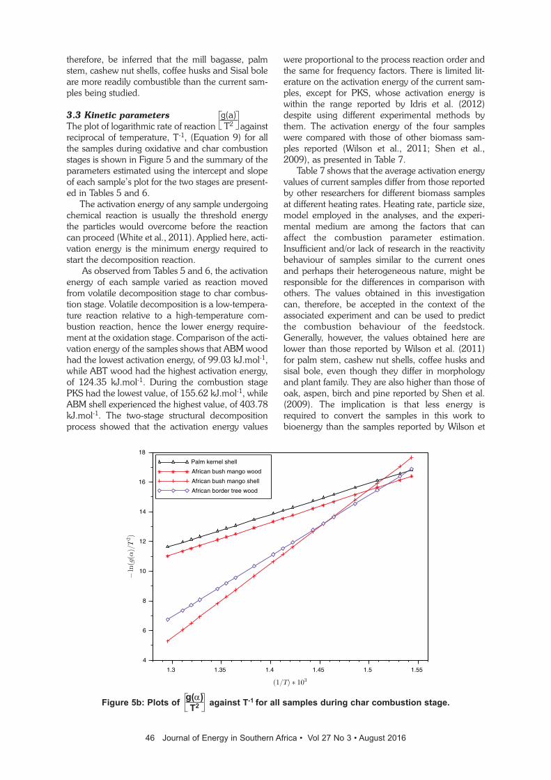
therefore, be inferred that the mill bagasse, palmstem, cashew nut shells, coffee husks and Sisal boleare more readily combustible than the current sam-ples being studied.
3.3 Kinetic parameters The plot of logarithmic rate of reaction againstreciprocal of temperature, T-1, (Equation 9) for allthe samples during oxidative and char combustionstages is shown in Figure 5 and the summary of theparameters estimated using the intercept and slopeof each sample’s plot for the two stages are present-ed in Tables 5 and 6.
The activation energy of any sample undergoingchemical reaction is usually the threshold energythe particles would overcome before the reactioncan proceed (White et al., 2011). Applied here, acti-vation energy is the minimum energy required tostart the decomposition reaction.
As observed from Tables 5 and 6, the activationenergy of each sample varied as reaction movedfrom volatile decomposition stage to char combus-tion stage. Volatile decomposition is a low-tempera-ture reaction relative to a high-temperature com-bustion reaction, hence the lower energy require-ment at the oxidation stage. Comparison of the acti-vation energy of the samples shows that ABM woodhad the lowest activation energy, of 99.03 kJ.mol-1,while ABT wood had the highest activation energy,of 124.35 kJ.mol-1. During the combustion stagePKS had the lowest value, of 155.62 kJ.mol-1, whileABM shell experienced the highest value, of 403.78kJ.mol-1. The two-stage structural decompositionprocess showed that the activation energy values
were proportional to the process reaction order andthe same for frequency factors. There is limited lit-erature on the activation energy of the current sam-ples, except for PKS, whose activation energy iswithin the range reported by Idris et al. (2012)despite using different experimental methods bythem. The activation energy of the four sampleswere compared with those of other biomass sam-ples reported (Wilson et al., 2011; Shen et al.,2009), as presented in Table 7.
Table 7 shows that the average activation energyvalues of current samples differ from those reportedby other researchers for different biomass samplesat different heating rates. Heating rate, particle size,model employed in the analyses, and the experi-mental medium are among the factors that canaffect the combustion parameter estimation.Insufficient and/or lack of research in the reactivitybehaviour of samples similar to the current onesand perhaps their heterogeneous nature, might beresponsible for the differences in comparison withothers. The values obtained in this investigationcan, therefore, be accepted in the context of theassociated experiment and can be used to predictthe combustion behaviour of the feedstock.Generally, however, the values obtained here arelower than those reported by Wilson et al. (2011)for palm stem, cashew nut shells, coffee husks andsisal bole, even though they differ in morphologyand plant family. They are also higher than those ofoak, aspen, birch and pine reported by Shen et al.(2009). The implication is that less energy isrequired to convert the samples in this work tobioenergy than the samples reported by Wilson et
46 Journal of Energy in Southern Africa • Vol 27 No 3 • August 2016
g(a)T2éë
ùû
1.41.3 1.51.35 1.45 1.55
10
4
6
8
12
14
16
18
Palm kernel shell
African bush mango wood
African bush mango shell
African border tree wood
Figure 5b: Plots of against T-1 for all samples during char combustion stage.g(a)T2éë
ùû
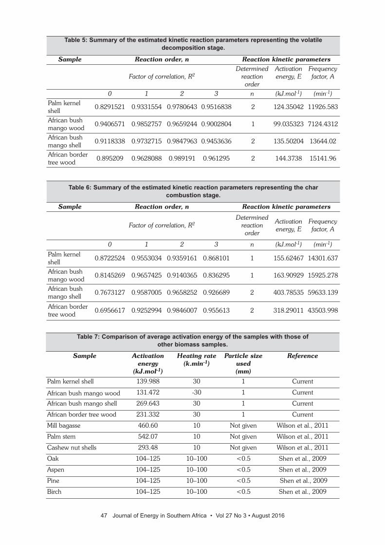
47 Journal of Energy in Southern Africa • Vol 27 No 3 • August 2016
Table 5: Summary of the estimated kinetic reaction parameters representing the volatiledecomposition stage.
Sample Reaction order, n Reaction kinetic parameters
Factor of correlation, R2Determined
reactionorder
Activationenergy, E
Frequencyfactor, A
0 1 2 3 n (kJ.mol-1) (min-1)Palm kernelshell 0.8291521 0.9331554 0.9780643 0.9516838 2 124.35042 11926.583
African bushmango wood 0.9406571 0.9852757 0.9659244 0.9002804 1 99.035323 7124.4312
African bushmango shell 0.9118338 0.9732715 0.9847963 0.9453636 2 135.50204 13644.02
African bordertree wood 0.895209 0.9628088 0.989191 0.961295 2 144.3738 15141.96
Table 6: Summary of the estimated kinetic reaction parameters representing the char combustion stage.
Sample Reaction order, n Reaction kinetic parameters
Factor of correlation, R2Determined
reactionorder
Activationenergy, E
Frequencyfactor, A
0 1 2 3 n (kJ.mol-1) (min-1)
Palm kernelshell 0.8722524 0.9553034 0.9359161 0.868101 1 155.62467 14301.637
African bushmango wood 0.8145269 0.9657425 0.9140365 0.836295 1 163.90929 15925.278
African bushmango shell 0.7673127 0.9587005 0.9658252 0.926689 2 403.78535 59633.139
African bordertree wood 0.6956617 0.9252994 0.9846007 0.955613 2 318.29011 43503.998
Table 7: Comparison of average activation energy of the samples with those of other biomass samples.
Sample Activationenergy
(kJ.mol-1)
Heating rate(k.min-1)
Particle sizeused(mm)
Reference
Palm kernel shell 139.988 30 1 Current
African bush mango wood 131.472 -30 1 Current
African bush mango shell 269.643 30 1 Current
African border tree wood 231.332 30 1 Current
Mill bagasse 460.60 10 Not given Wilson et al., 2011
Palm stem 542.07 10 Not given Wilson et al., 2011
Cashew nut shells 293.48 10 Not given Wilson et al., 2011
Oak 104–125 10–100 <0.5 Shen et al., 2009
Aspen 104–125 10–100 <0.5 Shen et al., 2009
Pine 104–125 10–100 <0.5 Shen et al., 2009
Birch 104–125 10–100 <0.5 Shen et al., 2009

al., but may require more energy than those report-ed by Shen et al. In addition to using different sam-ples from the ones reported by Wilson et al. andShen et al., geographical location, climatic condi-tions and biomass origin can contribute to the vari-ation in the parameters obtained.
4. ConclusionsThe combustion characteristics and decompositionkinetics of the biomass samples under oxidativeconditions were studied. The thermal decomposi-tion process showed distinctly the regions of mois-ture loss, structural decomposition and char com-bustion stages.
At the heating rate of 30 °C.min-1 the volatilerelease stage was the most critical of the degrada-tion process in all the samples because the greatermass loss was observed in this region, with theexception only of PKS. The greater combustion pro-cess of the samples, except for PKS, would, there-fore, most likely take place at this temperatureregion, with lower degree of combustion takingplace at the higher temperatures.
The samples were characterised by low activa-tion energies and decomposed at low energy inputcompared with some biomass samples reported inliterature under combustion conditions but differentheating rate and particle size. The samples also dis-played high reaction rates during the structuraldecomposition stages with high volatile release.
Under an oxygenated medium, the combustionprocesses of the samples was complete, leading tolow-carbon emission, which is a good attribute ofbiomass combustion for bioenergy production.
Owing to lack of reports on oxidative and com-bustion characteristics of the biomass samples stud-ied in this research, further investigation involvingvarying particle size, heating rates, pre-treatments,cultivation, location and biomass age (maturity) areproposed. This will not only provide additionalinformation on the combustion properties of thesamples but also validate the results presented inthis research.
References Ainge L. and Brown, N. Irvingia genensis and wombolu:
a state of knowledge report undertaken for theCentral African Regional program for the environ-ment. Oxford Forestry Institute, Department of PlantSciences, University of Oxford United Kingdom,2001. Online:http://carpe.umd.edu/Documents/2001/report-ainge-brown2001.pdf (accessed 23/3/2015).
Alvarez, E. and González, J. F. 1999. Combustion ofSpanish coals under simulated pressurized–fluidized-bed-combustion conditions. Fuel 78: 335–340.
Anyaoku, O. A. 2007. Nigerian bio-fuel policy andincentives, Official gazette of the Nigerian bio-fuelpolicy and incentives, Federal Republic of Nigeria.Online:
www.sunbirdbioenergy.com/docs/Nigeria_E10_POLI-CY_GAZETTED.pdf
Apaydin-Varol, E. Polat, S. and Putun, A. E. 2014.Pyrolysis kinetics and thermal decompositionbehaviour of polycarbonate – a TGA-FTIR study.Thermal Science 18(3): 833 – 842.
Ayuka, E. T., Duguma, B., Franzel, S., Kengue, J.,Mollet, M., Tiki-Manga, T. and Zenkeng, P. 1999.
Uses, management and economic potential of Irvingiagabonensis in the humid lowlands of Cameroon.Forest Ecology and Management 113(1): 1–9.
Bafor, E. and Sanni, U. 2009. Uterine contractile effectsof the aqueous and ethanol leaf extracts of newboul-dia laevis (Bignoniaceae) in vitro. Indian Journal ofPharmaceutical Science, 2009, 71(2):124–127.
Coats, A. W. and Redfern, J. P. 1964. Kinetic parame-ters from thermogravimetric data. Nature 201:68–69.
Conesa, J.A. and Rey, L. 2015. Thermogravimetric andkinetic analysis of the decomposition of solid recov-ered fuel from municipal solid waste, Journal ofThermal Analysis and Calorimetry. 120: 1233–1240.doi 10.1007/s10973-015-4396-4.
Department of Minerals and Energy. 2007. Biofuelsindustrial strategy of the Republic of South Africa,Online: www.energy.gov.za/files/esources/renew-ables/biofuels_indus_strat.pdf%282%29.pdf(accessed 09/02/2015).
Ejele, A.E., Enenebaku, C.K., Akujobi, C.O. and Ngwu,S.U. 2012. Effect of microbial spoilage on phyto-chemistry, antisickling and antimicrobial potential ofNewbouldia laevis leaf extract, InternationalResearch Journal of Microbiology 3(4):113-116.
El may, Y., Mejdi, J., Sophie D., Gwenaelle, T, andRachid, S. 2012. Study on the thermal behaviour ofdifferent date palm residues: characterization anddevolatilization kinetics under inert and oxidativeatmospheres. Energy 44: 702–709.http://dx.doi.org/10.1016/j.energy.2012.05.022.
Extension Bulletin. 1999. Production and utilization of‘ogbono, African bush mango’ (Irvingia gabonensis),Extension Bulletin no 140, Horticulture Series no 4.National Agricultural Extension and ResearchLiaison Services, Federal Ministry of Agriculture andWater Resources, ABU Zaria.
Ghetti, P., Leandro, R. and Luciana, A. 1966. Thermalanalysis of biomass and corresponding pyrolysisproducts. Fuel 75(5):565 – 573.
Idris, S. S., Rahman, N. A. and Ismail, K. 2012.Combustion characteristics of Malaysian oil palmbiomass, sub-bituminous coal and their respectiveblends via thermogravimetric analysis (TGA).Bioresource Technology 123:581–591.
Jeguirim, M., Bikai, J., El may, Y., Limousy, L., andNjeugna, E. 2014. Thermal characterization andpyrolysis kinetics of tropical biomass feedstocks forenergy recovery. Energy for SustainableDevelopment 23:188–193.
Lin, R., Zhu, Y. and Tavlarides, L.L. 2013. Mechanismand kinetics of thermal decomposition of biodieselfuel. Fuel 106:593–604.
Lu, J-J. and Chen, W-H. 2015. Investigation on theignition and burnout temperatures of bamboo and
48 Journal of Energy in Southern Africa • Vol 27 No 3 • August 2016

sugarcane bagasse by thermogravimetric analysis.Applied Energy 160:49–57.
Luangkiattikhun, P., Tangsathitkulchai, C. andTangsathitkulchai, M. 2008. Non-isothermal thermo-gravimetric analysis of oil-palm solid wastes.Bioresource Technology 99:986– 997.
Moon, C., Sung, Y., Eom, S. and Choi G. 2015. NOxemissions and burnout characteristics of bituminouscoal, lignite, and their blends in a pulverized coal-fired furnace. Experimental Thermal and FluidScience 62:99–108.
Munir, S., Daood, S. S., Nimmo, W., Cunliffe, A. M.and Gibbs, B. M. 2009. Thermal analysis anddevolatilization kinetics of cotton stalk, sugar canebagasse and shea meal under nitrogen and airatmospheres. Bioresource Technology 100:1413-1418.
Ninan, K. N. 1989. Kinetics of solid-state thermaldecomposition reactions, Journal of ThermalAnalysis 35:1267–1278.
Niu, Z., Liu, G., Yin, H., Wu, D. and Zhou, C. 2016.Investigation of mechanism and kinetics of non-isothermal low temperature pyrolysis of perhydrousbituminous coal by in-situ FTIR. Fuel 172:1–10.
Okoroigwe, E. C. Energy conversion of woody biomassby fast pyrolysis method. 2014. PhD dissertation.University of Nigeria, Nsukka, Nigeria.
Okoroigwe, E. C. and Saffron, C. M. 2012.Determination of bio-energy potential of palm kernelshell by physicochemical characterization. NigerianJournal of Technology. 31(3): 329–335.
Okpala, B. 2015. Incredible benefits of newbouldia lae-vis (ogilisi). Global food book. Online: http://global-foodbook.com/incredible-benefits-of-newbouldia-lae-vis-ogilisi/.
Park, S. W. and Jang, C. H. 2012. Effects of pyrolysistemperature on changes in fuel characteristics ofbiomass char. Energy 39:187 – 195.
Parthasarathy, P. Narayanan, K. S. and Arockiam, L.2013. Study on kinetic parameters of differentbiomass samples using thermo-gravimetric analysis.Biomass and Bioenergy 58:58–66.
Rainville, E. D. 1960. Special Functions. New York:Macmillan.
Roberts, M. J., Everson, R. C., Domazetis, G,Neomagus, H.W.J.P., Jones, J.M., Van Sittert,C.G.C.E., Okolo, G.N., Van Niekerk, D. andMathews, J. P. 2015. Density functional theorymolecular modelling and experimental particle kinet-ics for CO2–char gasification. Carbon 93:295–314.
Rostam-Abadi, M., DeBarr, J. A. and Moran, D. L.1988. Burning characteristics of partiallydevolatilized coals. Fuel Chemistry33:869-874.
Sahu, S. G., Sarkar, P., Chakraborty, N. and Adak, A. K.2010. Thermogravimetric assessment of combustioncharacteristics of blends of a coal with differentbiomass chars. Fuel Processing Technology91(3):369–378.
Shen, D. K., Gu, S., Luo, K. H., Bridgwater, A. V., andFang, M. X. 2009. Kinetic study on thermal decom-position of woods in oxidative environment. Fuel88:1024–1030.
Soccol, C. R., Vandenberghe, L. P. S., Costa, B.,
Woiciechowski, A. L., De Carvalho, J. C., MedeirosA. B. P., Franscisco, A. M. and Bonomi, L. J. 2005.Brazilian biofuel program: An overview. Journal ofScientic and Industrial Research 64(11):897–904.
Son, J. W. and Sohn, C. H. 2015. Evaluation ofburnout performance of biomass wastes in a rocket-engine-based incinerator. Fuel 143:308–317.
União Brasileira do Biodiesel e Bioquerosene (Ubrabio)and Getulio Vargas Foundation. 2010. Biodiesel andits contribution to Brazilian development, 1-34.Online:http://fgvenergia.fgv.br/sites/fgvenergia.fgv.br/files/ubrabio.pdf
Vamvuka, D. and Sfakiotakis, S. 2011. Combustionbehaviour of biomass fuels and their blends with lig-nite. Thermochimica Acta 526:192–199.
Wilson, L., Yang, W., Blasiak, W., John, G. R.and Mhilu,C. F. 2011. Thermal characterization of tropicalbiomass feedstocks, Energy Conversion andManagement 52:191–198.
Xiang-guo, L., Bao-guo, M., Li, X., Zhen-wu, H. andXin-gang, W. 2006. Thermogravimetric analysis ofthe co-combustion of the blends with high ash coaland waste tyres. Thermochimica Acta 441:79–83.
Zhang, D., Wall, T.F., and Tate, A.G. 1992. The reactivi-ty of pulverized coal char particles; experimentsusing ignition, burnout and DTG techniques andpartly burnt chars. Fuel 71:1247–1253.
49 Journal of Energy in Southern Africa • Vol 27 No 3 • August 2016

AbstractThe main objective of the present study is to rankSouth African provinces on the basis of incomingsolar radiation. The surface incident shortwave flux(SWFlux, Wm-2) of NASA Modern-Era RetrospectiveAnalysis for Research and Applications (MERRA2D) reanalysis data for the period 1980–2009 overSouth Africa was analysed on annual, seasonal andmonthly scales. The monthly mean ± standarddeviation values of SWFlux for the period revealedthat, Northern Cape received the most (267.38 ±4.32 Wm-2) incoming solar radiation throughout theyear, followed by North West (263.37 ± 7.13 Wm-
2) and Free State (259.20 ± 7.66 Wm-2). The north-ern region of Limpopo also showed a good amountof incoming solar radiation (257.95 ± 6.16 Wm-2)at the surface. KwaZulu-Natal received least(232.99 ± 7.02 Wm-2) amount of mean monthlysolar radiation in comparison with other provinces.On an annual scale, the Northern Cape ranked first,and on seasonal and monthly scales North Westranked first. Limpopo and Free State also per-formed well in the present study.
Keywords: solar radiation, solar energy, reanalysisdata
50
Journal of Energy in Southern Africa 27(3): 50–57
Corresponding author: Tel: +2712 367 6049 Email: [email protected]
Ranking South African provinces on the basis of MERRA2D surface incident shortwave flux
Jyotsna Singh*
South African Weather Service, 442 Rigel Avenue South, Erasmusrand, Pretoria, 0181, South Africa

1. IntroductionSolar radiation mainly reaches the earth’s surface inthe form of shortwave radiation. With a changingclimate, the amount of solar radiation reaching theearth’s surface is also changing. In this regard, themonitoring and analysis of solar radiation over aregion is important. Satellite data is good for theanalysis of solar radiation because of its better spa-tial coverage compared to the ground measure-ments.
The sun is also the source of solar energy.Efficient use of solar energy not only decreasesreliance on fossil fuels, but will also reduce environ-mental degradation associated with fossil fuels(Atilgan and Azapagic, 2015; Singh et al., 2011). Itsavailability over the earth’s surface varies fromplace to place due to factors including latitude, ele-vation and cloud cover. The geographic location ofSouth Africa is highly favorable for solar energy-based applications. Previous studies (Schulze andMcGee, 1976; Drummond and Vowinckel, 1957)indicate that over South Africa daily insolation mayreach up to 29 MJm-2. The population of SouthAfrica is over 50 million and to satisfy energydemand sustainably renewable energy is necessary.Development of any country’s renewable energypotential is important for sustainable development.Solar energy is considered as the most reliablerenewable energy resources (Kleissl, 2013). It isfreely available, but collecting and transforming it isnot very much cost-effective (Kougias et al., 2016).Means of collecting solar energy include photo-voltaic systems (PV), solar thermals (solar waterheaters, solar hot water panel, solar hot water col-lector), and solar thermal and PV working together.Before installing any solar energy collecting deviceat any site it is advisable to perform a detailed anal-ysis of the site, as any wrong information may leadto sub-optimal performance and unexpectedly pooreconomic returns. For example, the size and designof PV systems to be installed at any site should bedecided after proper solar resource assessment(Munzhebdi and Sebitosi, 2009). To assess a site’ssolar energy potential, long-term solar radiationdata is needed. Typical meteorological year (TMY)data have been also used in many solar resourceassessment studies (Kleissl, 2013) - that is, a long-term average of solar irradiance. TMY data, whichrepresent the typical conditions, might be less usefulwhere substantial variability and extremes in weath-er are observed.
While information related to incoming solarradiation is valuable, observational solar radiationdata is sparse. Radiometric stations provide data forsingle locations and sometime for a relatively shortduration. In this case, satellite data are reliablysourced. There is no doubt that in situ observationsare valuable but satellite data are arguably a betteroption due to their better spatial coverage. It is nec-
essary to understand the characteristics of datacarefully in order to use them for solar resourceassessment, as requirements for different projectsvary. The focus of solar radiation project on a PVinstallation requires mainly global horizontal irradi-ance (GHI) dataset, while concentrating solarpower needs a direct normal irradiance (DNI)dataset. For some solar projects, exceedance prob-abilities (P10, P50, P90, P95 and P99) of GHI andDNI are also calculated. The present study aims tostudy SWFlux, from MERRA 2D reanalysis data(1980–2009) over the nine provinces (see details inSection 2). SWFlux data were analysed in all theprovinces separately to understand its variation onprovincial scale. The provinces were also ranked onthe basis of available SWFlux. Studies based on rankare useful to convert large information intodigestible information and it is easier to rememberand present rank than actual values. In manyrenewable energy studies ranking method has beenused (Şengül et al, 2015; Mohamadabadi et al.2009; Goumas and Lygerou, 2000). Solar energystudies that focus on provinces can help govern-mental decision-making on a provincial scale. Thisstudy can also assist small-to-large solar energyinvestors, construction engineers, tourism industriesand architects to plan activities and make decisionsin their respective areas. It can also serve as a base-line for further studies related to solar energy poten-tial using MERRA 2D data.
2. Study area and datasetsSouth Africa lies between 22°–34° S latitude and16°–32° E longitude. On the west it is bounded bythe Atlantic Ocean; on the south and east by theIndian Ocean; on the North by Namibia, Botswanaand Zimbabwe; and by Mozambique and Swazi-land on the north-east. There are nine provinces:Free State, Northern Cape, Western Cape, Gau-teng, Mpumalanga, North West, Limpopo, Kwa-Zulu-Natal and Eastern Cape (Figure 1). There arefour primary climatic zones: desert (Northern Cape,North-Eastern parts of Western Cape); arid (Lim-
51 Journal of Energy in Southern Africa • Vol 27 No 3 • August 2016
Figure 1: The provinces of South Africa.
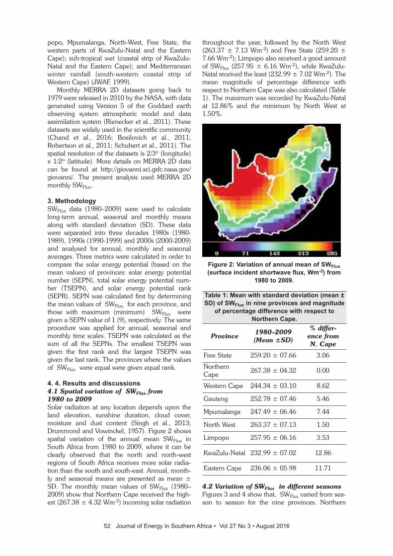
popo, Mpumalanga, North-West, Free State, thewestern parts of KwaZulu-Natal and the EasternCape); sub-tropical wet (coastal strip of KwaZulu-Natal and the Eastern Cape); and Mediterraneanwinter rainfall (south-western coastal strip ofWestern Cape) (JWAF, 1999).
Monthly MERRA 2D datasets going back to1979 were released in 2010 by the NASA, with datagenerated using Version 5 of the Goddard earthobserving system atmospheric model and dataassimilation system (Rienecker et al., 2011). Thesedatasets are widely used in the scientific community(Chand et al., 2016; Bosilovich et al., 2011;Robertson et al., 2011; Schubert et al., 2011). Thespatial resolution of the datasets is 2/3o (longitude)x 1/2o (latitude). More details on MERRA 2D datacan be found at http://giovanni.sci.gsfc.nasa.gov/giovanni/. The present analysis used MERRA 2Dmonthly SWFlux.
3. Methodology SWFlux data (1980–2009) were used to calculatelong-term annual, seasonal and monthly meansalong with standard deviation (SD). These datawere separated into three decades 1980s (1980-1989), 1990s (1990-1999) and 2000s (2000-2009)and analysed for annual, monthly and seasonalaverages. Three metrics were calculated in order tocompare the solar energy potential (based on themean values) of provinces: solar energy potentialnumber (SEPN), total solar energy potential num-ber (TSEPN), and solar energy potential rank(SEPR). SEPN was calculated first by determiningthe mean values of SWFlux for each province, andthose with maximum (minimum) SWFlux weregiven a SEPN value of 1 (9), respectively. The sameprocedure was applied for annual, seasonal andmonthly time scales. TSEPN was calculated as thesum of all the SEPNs. The smallest TSEPN wasgiven the first rank and the largest TSEPN wasgiven the last rank. The provinces where the valuesof SWFlux were equal were given equal rank.
4. 4. Results and discussions4.1 Spatial variation of SWFlux from 1980 to 2009Solar radiation at any location depends upon theland elevation, sunshine duration, cloud cover,moisture and dust content (Singh et al., 2013;Drummond and Vowinckel, 1957). Figure 2 showsspatial variation of the annual mean SWFlux inSouth Africa from 1980 to 2009, where it can beclearly observed that the north and north-westregions of South Africa receives more solar radia-tion than the south and south-east. Annual, month-ly and seasonal means are presented as mean ±SD. The monthly mean values of SWFlux (1980–2009) show that Northern Cape received the high-est (267.38 ± 4.32 Wm-2) incoming solar radiation
throughout the year, followed by the North West(263.37 ± 7.13 Wm-2) and Free State (259.20 ±7.66 Wm-2); Limpopo also received a good amountof SWFlux (257.95 ± 6.16 Wm-2), while KwaZulu-Natal received the least (232.99 ± 7.02 Wm-2). Themean magnitude of percentage difference withrespect to Northern Cape was also calculated (Table1). The maximum was recorded by KwaZulu-Natalat 12.86% and the minimum by North West at1.50%.
Figure 2: Variation of annual mean of SWFlux(surface incident shortwave flux, Wm-2) from
1980 to 2009.
4.2 Variation of SWFlux in different seasonsFigures 3 and 4 show that, SWFlux varied from sea-son to season for the nine provinces. Northern
52 Journal of Energy in Southern Africa • Vol 27 No 3 • August 2016
Table 1: Mean with standard deviation (mean ±SD) of SWFlux in nine provinces and magnitude
of percentage difference with respect toNorthern Cape.
Province 1980–2009(Mean ±SD)
% differ-ence from N. Cape
Free State 259.20 ± 07.66 3.06
NorthernCape 267.38 ± 04.32 0.00
Western Cape 244.34 ± 03.10 8.62
Gauteng 252.78 ± 07.46 5.46
Mpumalanga 247.49 ± 06.46 7.44
North West 263.37 ± 07.13 1.50
Limpopo 257.95 ± 06.16 3.53
KwaZulu-Natal 232.99 ± 07.02 12.86
Eastern Cape 236.06 ± 05.98 11.71

Cape showed more SWFlux in summer than anyother provinces, while Limpopo had more SWFlux inautumn (235 ± 4.61 Wm-2) and winter (201.60 ±4.7 Wm-2). During summer, autumn, winter andspring the maximum (minimum) SWFlux was inNorthern Cape, 357.57 ± 7.51 Wm-2 (KwaZulu-Natal, 288.714 ± 10.02 Wm-2), Limpopo, 235 ±4.61 Wm-2 (Eastern Cape, 199.74 ± 11.36 Wm-2),Limpopo, 201.60 ± 4.39 Wm-2 (Western Cape,141.31 ± 8.57 Wm-2), and Northern Cape, 310.40± 6.9 Wm-2 (KwaZulu-Natal, 264.41 ± 10.76 Wm-
2), respectively, as shown in Figure 4. Most areas inthe Northern Cape during the winter showed lessamount of SWFlux .The monthly mean of SWFluxwith SD for 1980–2009 in the nine provinces is pre-sented in Table 2, which shows that during the win-ter and autumn months Limpopo had higherSWFlux than other provinces. Present studies ofSWFlux results on annual and seasonal scale showsimilarity to the maps generated using the UnitedStates National Renewable Energy Laboratorydatabase (Fluri, 2009). These maps show that thesolar radiation was higher in Northern Cape duringsummer and spring and lower in winter. Themonthly mean values of SWFlux (1980-2009) withSD are presented in Table 2. In almost all theprovinces the SWFlux was higher in December andlower in June.
4.3 Spatial variation of SWFlux over threedecades SWFlux was analysed spatially over the threedecades of the datasets – the 1980s, 1990s and2000s (Figure 5). SWFlux in Northern Cape washigher than in any other province in all three
53 Journal of Energy in Southern Africa • Vol 27 No 3 • August 2016
Figure 3: Climatological mean of monthly means of SWFlux (surface shortwave incident flux, W/m2) from MERRA 2D reanalysis (1980–2009), by season.
Figure 4: Seasonal variation of surface incidentshortwave flux (SWFlux), Wm-2 in the nine
provinces of South Africa. (FS, NC, WC, GT, MP,NW, LP, KZN and EC stand respectively for FreeState, Northern Cape, Western Cape, Gauteng,Mpumalanga, North West, Limpopo, KwaZulu-
Natal and Eastern Cape).

54 Journal of Energy in Southern Africa • Vol 27 No 3 • August 2016
Table 2: Monthly mean of surface incident shortwave flux, Wm-2 with a standard deviation (SD) for 1980–2009in the nine provinces of South Africa.
SWFlux (Mean ±SD)
Province Jan Feb Mar Apr May June
Free State 334.45 ± 16.57 305.80 ± 8.36 270.28 ± 3.97 225.09 ± 3.60 184.94 ± 5.54 163.31 ± 6.03
Northern Cape 366.74 ± 8.41 330.39 ± 7.31 279.72 ± 5.12 223.46 ± 8.61 177.27 ± 11.56 153.94 ± 12.59
Western Cape 359.65 ± 11.46 319.92 ± 12.70 261.91 ± 11.65 195.73 ± 9.81 145.71 ± 8.77 121.94 ± 7.84
Gauteng 297.93 ± 5.37 285.93 ± 2.90 260.82 ± 2.99 229.67 ± 1.06 197.02 ± 1.28 177.01 ± 1.82
Mpumalanga 325.53 ± 3.14 286.72 ± 3.87 258.23 ± 3.32 224.53 ± 4.35 192.55 ± 4.25 173.56 ± 4.29
North West 325.53± 16.50 300.26 ± 9.77 271.14 ± 5.73 234.22 ± 2.37 196.98 ± 3.30 175.69 ± 3.47
Limpopo 304.72 ± 2.70 294.37 ± 4.39 267.59 ± 4.38 234.93 ± 4.91 202.48 ± 4.54 183.21 ± 3.82
KwaZulu-Natal 291.84 ± 9.83 277.56 ± 8.78 246.21 ± 8.77 207.06 ± 8.52 172.13 ± 7.85 152.87 ± 7.38
Eastern Cape 324.41 ± 19.17 291.27 ± 14.21 248.47 ± 11.67 196.00 ± 11.11 154.00 ± 11.30 133.03 ± 11.02
July Aug Sept Oct Nov Dec
Free State 174.53 ± 6.16 212.17 ± 4.76 264.44 ± 3.74 299.65 ± 6.32 331.56 ± 12.86 344.23 ± 17.85
Northern Cape 164.82 ± 12.07 205.33 ± 11.80 261.02 ± 9.65 314.41 ± 5.65 355.76 ± 5.43 375.58 ± 6.81
Western Cape 131.78 ± 8.61 170.58 ± 9.26 229.78 ± 9.41 291.69 ± 10.39 338.63 ± 10.43 365.10 ± 11.00
Gauteng 187.96 ± 1.69 223.07 ± 1.51 270.49 ± 0.99 294.46 ± 2.04 305.63 ± 5.79 303.35 ± 7.13
Mpumalanga 183.88 ± 04.68 217.58 ± 05.28 261.84 ± 06.38 284.33 ± 06.24 293.24 ± 06.74 295.68 ± 05.96
North West 186.90 ± 03.50 223.97 ± 02.80 273.58 ± 02.06 305.86 ± 04.94 330.08 ± 13.18 336.19± 18.52
Limpopo 193.37 ± 04.33 228.22 ± 05.04 272.31 ± 05.95 301.59 ± 06.48 306.96 ± 6.84 305.62 ± 5.29
KwaZulu-Natal 162.67 ± 08.01 195.61 ± 09.17 238.45 ± 11.29 267.42 ± 09.56 287.35 ± 11.42 296.75 ± 11.45
Eastern Cape 143.85 ± 11.42 179.89 ± 12.80 231.28 ± 13.11 279.38 ± 12.91 316.07 ± 14.82 334.25 ± 18.46
Figure 5: Spatial variation of SWFlux (surface incident shortwave flux, Wm-2) in the last threedecades over South Africa.
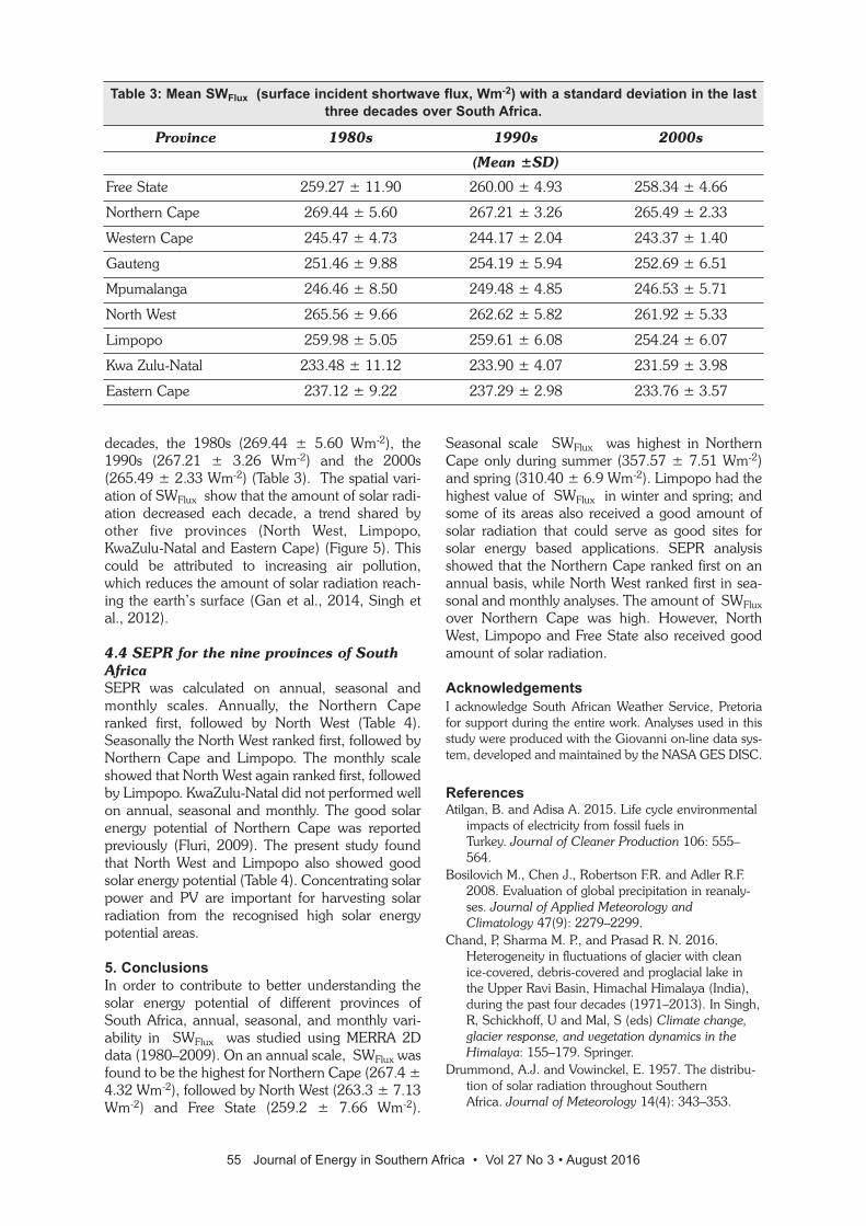
decades, the 1980s (269.44 ± 5.60 Wm-2), the1990s (267.21 ± 3.26 Wm-2) and the 2000s(265.49 ± 2.33 Wm-2) (Table 3). The spatial vari-ation of SWFlux show that the amount of solar radi-ation decreased each decade, a trend shared byother five provinces (North West, Limpopo,KwaZulu-Natal and Eastern Cape) (Figure 5). Thiscould be attributed to increasing air pollution,which reduces the amount of solar radiation reach-ing the earth’s surface (Gan et al., 2014, Singh etal., 2012).
4.4 SEPR for the nine provinces of SouthAfricaSEPR was calculated on annual, seasonal andmonthly scales. Annually, the Northern Caperanked first, followed by North West (Table 4).Seasonally the North West ranked first, followed byNorthern Cape and Limpopo. The monthly scaleshowed that North West again ranked first, followedby Limpopo. KwaZulu-Natal did not performed wellon annual, seasonal and monthly. The good solarenergy potential of Northern Cape was reportedpreviously (Fluri, 2009). The present study foundthat North West and Limpopo also showed goodsolar energy potential (Table 4). Concentrating solarpower and PV are important for harvesting solarradiation from the recognised high solar energypotential areas.
5. ConclusionsIn order to contribute to better understanding thesolar energy potential of different provinces ofSouth Africa, annual, seasonal, and monthly vari-ability in SWFlux was studied using MERRA 2Ddata (1980–2009). On an annual scale, SWFlux wasfound to be the highest for Northern Cape (267.4 ±4.32 Wm-2), followed by North West (263.3 ± 7.13Wm-2) and Free State (259.2 ± 7.66 Wm-2).
Seasonal scale SWFlux was highest in NorthernCape only during summer (357.57 ± 7.51 Wm-2)and spring (310.40 ± 6.9 Wm-2). Limpopo had thehighest value of SWFlux in winter and spring; andsome of its areas also received a good amount ofsolar radiation that could serve as good sites forsolar energy based applications. SEPR analysisshowed that the Northern Cape ranked first on anannual basis, while North West ranked first in sea-sonal and monthly analyses. The amount of SWFluxover Northern Cape was high. However, NorthWest, Limpopo and Free State also received goodamount of solar radiation.
AcknowledgementsI acknowledge South African Weather Service, Pretoriafor support during the entire work. Analyses used in thisstudy were produced with the Giovanni on-line data sys-tem, developed and maintained by the NASA GES DISC.
ReferencesAtilgan, B. and Adisa A. 2015. Life cycle environmental
impacts of electricity from fossil fuels inTurkey. Journal of Cleaner Production 106: 555–564.
Bosilovich M., Chen J., Robertson F.R. and Adler R.F.2008. Evaluation of global precipitation in reanaly-ses. Journal of Applied Meteorology andClimatology 47(9): 2279–2299.
Chand, P, Sharma M. P., and Prasad R. N. 2016.Heterogeneity in fluctuations of glacier with cleanice-covered, debris-covered and proglacial lake inthe Upper Ravi Basin, Himachal Himalaya (India),during the past four decades (1971–2013). In Singh,R, Schickhoff, U and Mal, S (eds) Climate change,glacier response, and vegetation dynamics in theHimalaya: 155–179. Springer.
Drummond, A.J. and Vowinckel, E. 1957. The distribu-tion of solar radiation throughout SouthernAfrica. Journal of Meteorology 14(4): 343–353.
55 Journal of Energy in Southern Africa • Vol 27 No 3 • August 2016
Table 3: Mean SWFlux (surface incident shortwave flux, Wm-2) with a standard deviation in the lastthree decades over South Africa.
Province 1980s 1990s 2000s
(Mean ±SD)
Free State 259.27 ± 11.90 260.00 ± 4.93 258.34 ± 4.66
Northern Cape 269.44 ± 5.60 267.21 ± 3.26 265.49 ± 2.33
Western Cape 245.47 ± 4.73 244.17 ± 2.04 243.37 ± 1.40
Gauteng 251.46 ± 9.88 254.19 ± 5.94 252.69 ± 6.51
Mpumalanga 246.46 ± 8.50 249.48 ± 4.85 246.53 ± 5.71
North West 265.56 ± 9.66 262.62 ± 5.82 261.92 ± 5.33
Limpopo 259.98 ± 5.05 259.61 ± 6.08 254.24 ± 6.07
Kwa Zulu-Natal 233.48 ± 11.12 233.90 ± 4.07 231.59 ± 3.98
Eastern Cape 237.12 ± 9.22 237.29 ± 2.98 233.76 ± 3.57

Earth data, Giovanni. http://giovanni.sci.gsfc.nasa.gov/giovanni/ (Retrieved on June, 2015).
Fluri, T.P. The potential of concentrating solar power inSouth Africa. 2009. Energy Policy 37(12): 5075–5080.
Gan, C.M., Pleim, J., Mathur, R., Hogrefe, C., Long,C.N., Xing, J., Roselle, S. and Wei, C. 2014Assessment of the effect of air pollution controls ontrends in shortwave radiation over the United Statesfrom 1995 through 2010 from multiple observationnetworks. Atmospheric Chemistry and Physics 14(3):1701–1715.
Goumas, M., and V. Lygerou. 2000. An extension of thePROMETHEE method for decision making in fuzzyenvironment: Ranking of alternative energy exploita-tion projects. European Journal of OperationalResearch 123(3): 606–613.
JAWF (Joint Agricultural Weather Facility), 1999. Majorworld crop areas and climate profiles. www.usda.gov/oce/waob/jawf/profiles/mwcacp2.htm (Retrievedon May, 2015).
Kleissl, J. 2013. Solar energy forecasting and resourceassessment. Academic Press.
Kougias, I., Szabó, S., Monforti-Ferrario, F., Huld, T. andBódis, K. 2016. Methodology for optimization of thecomplementarity between small-hydropower plantsand solar PV systems. Renewable Energy 87: 1023–1030.
Mohamadabadi, H. Safaei, G. Tichkowsky, and A.Kumar. 2009. Development of a multi-criteria assess-ment model for ranking of renewable and non-renewable transportation fuel vehicles. Energy 34(1):112–125.
Munzhedzi, R. and Sebitosi, A.B. 2009. Redrawing the
56 Journal of Energy in Southern Africa • Vol 27 No 3 • August 2016
Table 4: Solar energy potential number (SEPN), total solar energy potential number (TSEPN), andsolar energy potential rank (SEPR) on annual, seasonal and monthly scales in the nine provinces
of South Africa.
Free State
N. Cape
W. Cape
Gau-teng
Mpuma-langa
North West
Lim-popo
KwaZulu-Natal
E. Cape
SEPNAnnual 3 1 7 5 6 2 4 9 8
TSEPNAnnual 3 1 7 5 6 2 4 9 8
SEPRAnnual 3 1 7 5 6 2 4 9 8
SEPNSummer 3 1 2 7 8 4 6 9 5
SEPNAutumn 5 4 8 3 6 2 1 7 9
SEPNWinter 5 6 9 2 4 3 1 7 8
SEPNSpring 3 1 6 5 7 2 4 9 8
TSEPNSeasonal 16 12 25 17 25 11 12 32 30
SEPRSeasonal 3 2 5 4 5 1 2 7 6
SEPNJan 3 1 2 7 8 4 6 9 5
SEPNFeb 3 1 2 8 7 4 5 9 6
SEPNMar 3 1 5 6 7 2 4 9 8
SEPNApril 4 6 9 3 5 2 1 7 8
SEPNMay 5 6 9 2 4 3 1 7 8
SEPNJune 5 6 9 2 4 3 1 7 8
SEPNJuly 5 6 9 2 4 3 1 7 8
SEPNAug 5 6 9 3 4 2 1 7 8
SEPNSpet 4 6 9 3 5 1 2 7 8
SEPNOct 4 1 6 5 7 2 3 9 8
SEPNNov 3 1 2 7 8 4 6 9 5
SEPNDec 3 1 2 7 9 4 6 8 5
TSEPNMonthly 47 42 73 55 72 34 37 95 85
SEPRMonthly 4 3 7 5 6 1 2 9 8

solar map of South Africa for photovoltaic applica-tions. Renewable Energy 34(1):165–169.
Rienecker, M.M., Suarez, M.J., Gelaro, R., Todling, R.,Bacmeister, J., Liu, E., Bosilovich, M.G., Schubert,S.D., Takacs, L., Kim, G.K. and Bloom, S. 2011.MERRA: NASA’s modern-era retrospective analysisfor research and applications. Journal of Climate24(14): 3624–3648.
Robertson, F.R., Bosilovich, M.G., Chen, J. and Miller,T.L. 2011. The effect of satellite observing systemchanges on MERRA water and energyfluxes. Journal of Climate 24(20): 5197–5217.
Schulze, R. E., and O. S. McGee. 1976. Winter andsummer insolation patterns for SouthernAfrica. South African Journal of Science, 72:182-183.
Schubert, S., Wang, H. and Suarez, M. 2011. Warmseason subseasonal variability and climate extremesin the northern hemisphere: The role of stationaryRossby waves. Journal of Climate 24(18): 4773–4792.
Şengül, Ü., Eren, M., Shiraz, S.E., Gezder, V. andŞengül, A.B. 2015. Fuzzy TOPSIS method for rank-ing renewable energy supply systems inTurkey. Renewable Energy 75: 617–625.
Singh, J., Kumar, M. and Bhattacharya, B.K. 2011.Solar energy potential of two metropolitan cities ofIndia. In Pradhan, R.P. (ed). Infrastructure – the keyto development. Proceedings of InternationalConference on Infrastructure Finance (ICIF 2010)held jointly by Vinod Gupta School of Managementand RCG School of Infrastructure Design andManagement, Indian Institute of TechnologyKharagpur on June 03-05, 2010. Macmillan India.
.Singh, J., Bhattacharya, B.K., Kumar, M. and Mallick,K. 2013. Modelling monthly diffuse solar radiationfraction and its validity over the Indian sub-tropics.International Journal of Climatology 33(1):77–86.
Singh, J., Bhattacharya, B. K., Kumar, M. 2012. SolarRadiation and Evaporation Trend overIndia. Journal of Earth Science and Engineering,2(3): 160-165.
57 Journal of Energy in Southern Africa • Vol 27 No 3 • August 2016