VOLUME 4 GEOTECHNICS AND DRAINAGE SECTION 2 · PDF fileVOLUME 4 GEOTECHNICS AND DRAINAGE ... for a given frequency of ... of rainfall intensity with storm duration. HD 33: Design of

November 2017

DESIGN MANUAL FOR ROADS AND BRIDGES

VOLUME 4 GEOTECHNICS AND DRAINAGE

SECTION 2 DRAINAGE

PART 4

HA 37/17

HYDRAULIC DESIGN OF ROAD-EDGE SURFACE WATER CHANNELS

SUMMARY

This Advice Note describes a method of determining the length of road between outlets that can be drained by a given size of surface water channel constructed along the edge of the road. The design method can be used for channels of triangular, rectangular or trapezoidal cross section.

INSTRUCTIONS FOR USE

1. Remove existing Contents pages for Volume 4.

2. Insert new Contents pages for Volume 4, dated November 2017.

3. Remove HA 37/97 from Volume 4, Section 2.

4. Insert HA 37/17 into Volume 4, Section 2, Part 4.

5. Archive this sheet as appropriate.

Note: A quarterly index with a full set of Volume Contents Pages is available separately from The Stationery Office Ltd.


Summary: This Advice Note describes a method of determining the length of road between outlets that can be drained by a given size of surface water channel constructed along the edge of the road. The design method can be used for channels of triangular, rectangular or trapezoidal cross section.

Hydraulic Design of Road-edge Surface Water Channels

HA 37/17 Volume 4, Section 2, Part 4

HIGHWAYS ENGLAND

TRANSPORT SCOTLAND

LLYWODRAETH CYMRUWELSH GOVERNMENT

DEPARTMENT FOR INFRASTRUCTURE NORTHERN IRELAND

November 2017

Registration of AmendmentsVolume 4 Section 2Part 4 HA 37/17

Amend No Page No Signature & Date of incorporation of amendments


REGISTRATION OF AMENDMENTS

November 2017

Registration of AmendmentsVolume 4 Section 2

Part 4 HA 37/17



REGISTRATION OF AMENDMENTS

November 2017


VOLUME 4 GEOTECHNICS AND DRAINAGE

SECTION 2 DRAINAGE

PART 4

HA 37/17

HYDRAULIC DESIGN OF ROAD-EDGE SURFACE WATER CHANNELS

Contents

Chapter

1. Introduction

2. Scope

3. Safety Aspects

4. Basis of Design Method

5. Description of Design Equations

6. Storm Return Period

7. Geographical Location

8. Channel Geometry

9. Channel Gradient

10. Drainage Length

11. Channel Roughness

12. Catchment Width

13. Surcharged Channels

14. By-Passing at Outlets

15. Construction Tolerances

16. Worked Examples

17. Glossary of Symbols

18. References

19. Approval

Annex A Rainfall data

Annex B Channel roughness

Annex C Run-off from cuttings

Annex D List of Amendments from Previous Version

November 2017 1/1

Chapter 1Introduction

Volume 4 Section 2Part 4 HA 37/17

1. INTRODUCTION1.1 Background

In the United Kingdom there are three main methods of dealing with surface run-off from rural trunk roads: combined surface and sub-surface drains; kerbs and gullies connecting to pipes below ground; and surface water channels along the pavement edge.

The term “Roads” used in Scotland and Northern Ireland is synonymous with the term “Highways” defined in the Highways Act 1980. In this document the term highway will be used as the standard terminology, however for clarity, where the term “roads” is used in this document, it should be taken to be equivalent to “highway”.

This document provides advice on the hydraulic design of surface water channels and should treated as such in the design of new schemes.

The use of surface water channels allows larger distances between outlets than conventional gully systems, and the positions of the outlets can often be chosen to suit the local topography and the occurrence of natural watercourses. With this type of system, seepage flows in the pavement construction are usually drained by means of fin or narrow filter drains at the edge of the pavement. Geometric and performance requirements for surface water channels and fin drains are given in Volumes 1 to 3 of the Manual of Contract Documents for Highway Works (MCHW 1, 2 & 3) (ref 1) and in HA 39, Edge of Pavement Details (DMRB 4.2).

In order to design a surface water channel for a given frequency of flooding, it is necessary to take account of the time of travel of flow along the channel and the variation of rainfall intensity with storm duration. HD 33: Design of Highway Drainage Systems (DMRB 4.2) states the adjustments to design rainfall intensities to account for Climate Change. The design method described in this document is obtained by combining results from kinematic wave theory about time-varying flow conditions in channels with UK rainfall characteristics. The validity of kinematic wave theory for flows in shallow drainage channels was checked using measurements from a trial on the M6 motorway [Ref 6].

The hydraulic design guidance contained in this document utilises a rainfall formula that has been optimised for storm durations between two minutes and twenty minutes; this range covers the great majority of applications. The design method has been generalized so that it can additionally now be applied to channels of trapezoidal cross-section. The results are presented in the form of equations instead of graphs so as to allow a simpler calculation procedure that is also suitable for use in computer-based design packages.

Further guidance on the design of grassed surface water channels is contained in HA 119: Grassed Surface Water Channels for Highway Runoff (DMRB 4.2) (Ref 2)

1.2 Scope and Purpose

The principles outlined in this Advice Note apply to all schemes on motorways and all-purpose trunk roads. The scope of this document is defined in Section 2

Design Policy

HD 49: Highway Drainage Design Principal Requirements (DMRB 4.2) (Ref 2) describes the policy for the selection and design of road drainage systems for sustainability and the relevant legislation. The design of drainage systems for all trunk roads and motorways in England and Wales is subject to certification and specific guidance on the certification process is given HD50: The Certification of Drainage Design (DMRB 4.2).


1/2 November 2017



Recording of asset inventory and condition data

Data regarding the inventory and condition of the drainage assets described in this document, and their connectivity with the rest of the drainage system, is to be uploaded and maintained in the drainage data management system described in HD 33 Chapter 10 (DMRB 4.2). All continuous assets must be connected to a point asset at each end, with one point defined as upstream and the other as downstream.

Surface water channels are recorded as continuous assets with the appropriate item type. In addition to the recommended attributes for all continuous assets, particular attention should be given to recording overall dimensions of the channel, invert levels, the shape of the cross-section, and the location of the channel within the highway cross-section. Further details such as a diagram of the cross-section may be attached to the record as a document.

This is applicable to England and Wales only; for Northern Ireland and Scotland consult the relevant Overseeing Organisation.

1.3 Definitions,AcronymsandAbbreviations

The definitions of the various drainage asset types are contained in HD43 (DMRB 4.2) whereas environmental definitions are contained in HD45 (DMRB 11)

A glossary of symbols used in this document is contained in Section 7.

1.4 Equality Impact Assessments

This document shall be implemented in accordance with GD1. An assessment as to the applicability of an equality impact assessment (EqIA) shall be carried out for all designs. Where the assessment indicates that an EqIA is required, then the designer shall carry out an EqIA.

1.5 Devolved Administrations

In Northern Ireland, this Advice Note will be applicable to those roads designated by the Department for Infrastructure Northern Ireland.

1.6 Implementation

This Advice Note should be used forthwith for all schemes currently being prepared provided that, in the opinion of the Overseeing Organisation, this would not result in significant additional expense or delay progress. Design Organisations should confirm its application to particular schemes with the Overseeing Organisation (see HD 33 – DMRB 4.2).

1.7 Assumptions made in the preparation of the Document

Guidance is given on the basic assumption that the works will be constructed in accordance with the MCHW. Assumptions relate to hydraulic flow properties in channels and on the permeability of surfaces being drained.

1.8 Feedback and Enquiries

Users of this document are encouraged to raise any enquiries and/or provide feedback on its contents and usage to the dedicated HE team. The email address for all enquiries and feedback is: [email protected]

November 2017 2/1

Chapter 2Scope


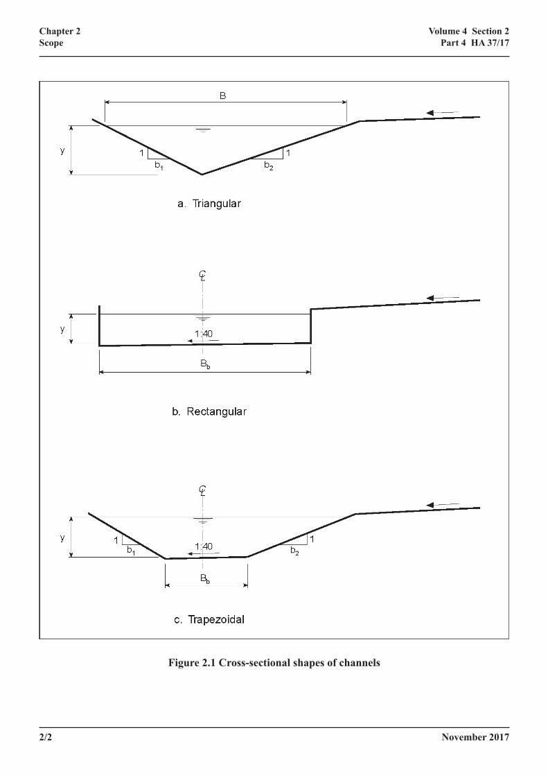
2. SCOPE2.1 This Advice Note describes a method of determining the length of road that can be drained by a given size

of surface water channel constructed along the edge of the road between outlets. The design method can be used for channels of triangular, rectangular or trapezoidal cross-section (see Figure 2 1), and is based on application of Equation (13) in paragraph 5.3.

2.2 Safety considerations limit the depth and types of cross-sectional shape that may be used for surface water channels which are not segregated from traffic. Permitted dimensions and cross-falls given in the 500 Series of MCHW1 (ref 1) and HA 39 (DMRB 4.2) are summarized in Chapter 3.

2.3 In the design method, the longitudinal gradient of a channel may either be constant or vary with distance. In the latter case, the gradient can be zero at the upstream or downstream end of the channel, but at all intermediate points there must be a positive fall towards the outlet. An approximate procedure is also given for checking the performance of channels when they are surcharged.

2.4 The design equations are based on assumptions that the cross-sectional properties of a channel do not vary with distance or depth of flow and that the width of road drained between two adjacent outlets is constant. If these assumptions are not satisfied, approximate results may be obtained using average values of road width or cross- sectional shape.

2.5 The design of outlets for use with surface water channels is described in HA 78, Design of Outlets for Surface Water Channels (DMRB 4.2).

2/2 November 2017

Chapter 2Scope


Figure 2.1 Cross-sectional shapes of channels

November 2017 3/1

Chapter 3Safety Aspects


3. SAFETY ASPECTS3.1 When considering the use of surface water channels, in particular those of rectangular cross-section, safety

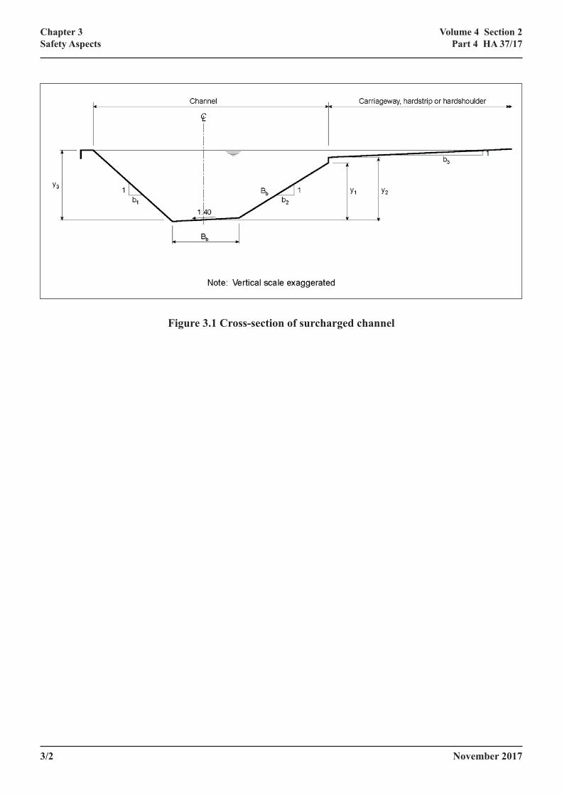
aspects relating to their location should be taken into account. Triangular or trapezoidal channels will usually be sited adjacent to the hardstrip or hardshoulder or at the edge of the carriageway and in front of the road restraint barrier, where one is provided; general layouts are given in the ‘A’ and ‘B’ Series of the Highway Construction Details (HCD) (MCHW 3). In these locations the maximum design depth of flow (dimension y1 in Figure 3.1) should be limited to 150mm. In both verges and central reserves the channel slopes (1:b1 and 1:b2 in Figure 3.1) should not be steeper than 1:5 for triangular channels and 1:4.5 for trapezoidal channels; in very exceptional cases slopes of 1:4 are allowable for both types of channel.

3.2 Rectangular channels, or triangular channels of depth greater than 150mm, should be used only where a barrier is provided between the channel and the carriageway; such channels can, therefore, normally only be justified where a barrier is warranted by other considerations. In addition, these channels should not be located in the barrier deflection zone into which the barrier is designed to deflect on vehicle impact. Shallower channels as described in paragraph 3.1 may lie in this deflection zone, or be crossed by the barrier (usually at a narrow angle) provided that the combined layout complies with the requirement of TD 19: Requirements for Road Restraint Systems, (DMRB 2.2)and the HCD (MCHW 3). Further advice on such layouts should be sought from the Overseeing Department. in terms of set-back and clearance dimensions and the mounting height of the barrier.

3.3 Co-ordination of the barrier and surface water channel layout should be arranged at an early stage in design and not left to compromise at later stages. Where barriers are not immediately deemed necessary, sufficient space should be provided in the verge or central reserve to allow for their possible installation. The combined layout must comply with the requirements of TD 19 and the HCD in terms of set-back and clearance dimensions and the mounting height of the safety fence.

3.4 The geometric constraints given in this document should also be applied to channel outfall details. In outfall design and at other channel terminations, slopes exceeding 1:4 should not be used on any faces, particularly those orthogonal to the direction of traffic, unless such faces are behind a barrier.

3/2 November 2017

Chapter 3Safety Aspects


Figure 3.1 Cross-section of surcharged channel

November 2017 4/1

Chapter 4Basis of Design Method


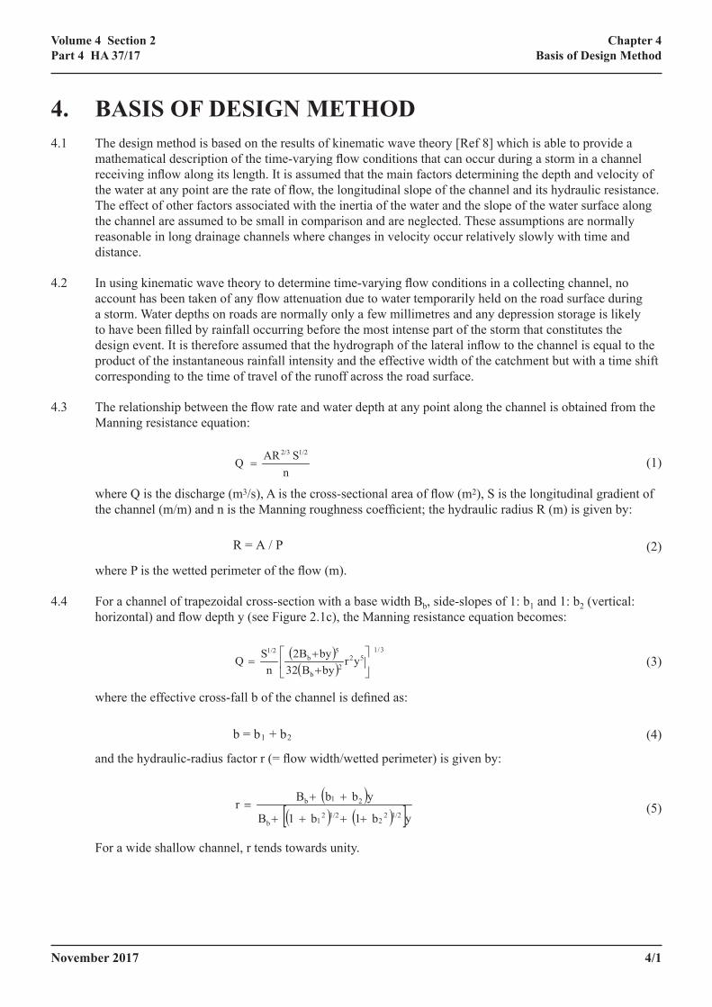
4. BASIS OF DESIGN METHOD4.1 The design method is based on the results of kinematic wave theory [Ref 8] which is able to provide a

mathematical description of the time-varying flow conditions that can occur during a storm in a channel receiving inflow along its length. It is assumed that the main factors determining the depth and velocity of the water at any point are the rate of flow, the longitudinal slope of the channel and its hydraulic resistance. The effect of other factors associated with the inertia of the water and the slope of the water surface along the channel are assumed to be small in comparison and are neglected. These assumptions are normally reasonable in long drainage channels where changes in velocity occur relatively slowly with time and distance.

4.2 In using kinematic wave theory to determine time-varying flow conditions in a collecting channel, no account has been taken of any flow attenuation due to water temporarily held on the road surface during a storm. Water depths on roads are normally only a few millimetres and any depression storage is likely to have been filled by rainfall occurring before the most intense part of the storm that constitutes the design event. It is therefore assumed that the hydrograph of the lateral inflow to the channel is equal to the product of the instantaneous rainfall intensity and the effective width of the catchment but with a time shift corresponding to the time of travel of the runoff across the road surface.

4.3 The relationship between the flow rate and water depth at any point along the channel is obtained from the Manning resistance equation:

n

S AR Q1/22/3

=

R = A / P

( )( )

++

= 522

b

5b

1/2

yrbyB32by2B

nSQ

3/1

b = b1 + b2

( )

( ) ( )[ ]yb1b1B

ybbBr1/22

21/22

1b

21b

++++

++=

=

32yr

nbSQ

821/2 3/1

( ) ( )1/222

1/221

21

b1b1

bbr+++

+=

(1)

where Q is the discharge (m3/s), A is the cross-sectional area of flow (m2), S is the longitudinal gradient of the channel (m/m) and n is the Manning roughness coefficient; the hydraulic radius R (m) is given by:

n

S AR Q1/22/3

=

R = A / P

( )( )

++

= 522

b

5b

1/2

yrbyB32by2B

nSQ

3/1

b = b1 + b2

( )

( ) ( )[ ]yb1b1B

ybbBr1/22

21/22

1b

21b

++++

++=

=

32yr

nbSQ

821/2 3/1

( ) ( )1/222

1/221

21

b1b1

bbr+++

+=

(2)

where P is the wetted perimeter of the flow (m).

4.4 For a channel of trapezoidal cross-section with a base width Bb, side-slopes of 1: b1 and 1: b2 (vertical: horizontal) and flow depth y (see Figure 2.1c), the Manning resistance equation becomes:

n

S AR Q1/22/3

=

R = A / P

( )( )

++

= 522

b

5b

1/2

yrbyB32by2B

nSQ

3/1

b = b1 + b2

( )

( ) ( )[ ]yb1b1B

ybbBr1/22

21/22

1b

21b

++++

++=

=

32yr

nbSQ

821/2 3/1

( ) ( )1/222

1/221

21

b1b1

bbr+++

+=

(3)

where the effective cross-fall b of the channel is defined as:

n

S AR Q1/22/3

=

R = A / P

( )( )

++

= 522

b

5b

1/2

yrbyB32by2B

nSQ

3/1

b = b1 + b2

( )

( ) ( )[ ]yb1b1B

ybbBr1/22

21/22

1b

21b

++++

++=

=

32yr

nbSQ

821/2 3/1

( ) ( )1/222

1/221

21

b1b1

bbr+++

+=

(4)

and the hydraulic-radius factor r (= flow width/wetted perimeter) is given by:

n

S AR Q1/22/3

=

R = A / P

( )( )

++

= 522

b

5b

1/2

yrbyB32by2B

nSQ

3/1

b = b1 + b2

( )

( ) ( )[ ]yb1b1B

ybbBr1/22

21/22

1b

21b

++++

++=

=

32yr

nbSQ

821/2 3/1

( ) ( )1/222

1/221

21

b1b1

bbr+++

+=

(5)

For a wide shallow channel, r tends towards unity.

4/2 November 2017

Chapter 4Basis of Design Method


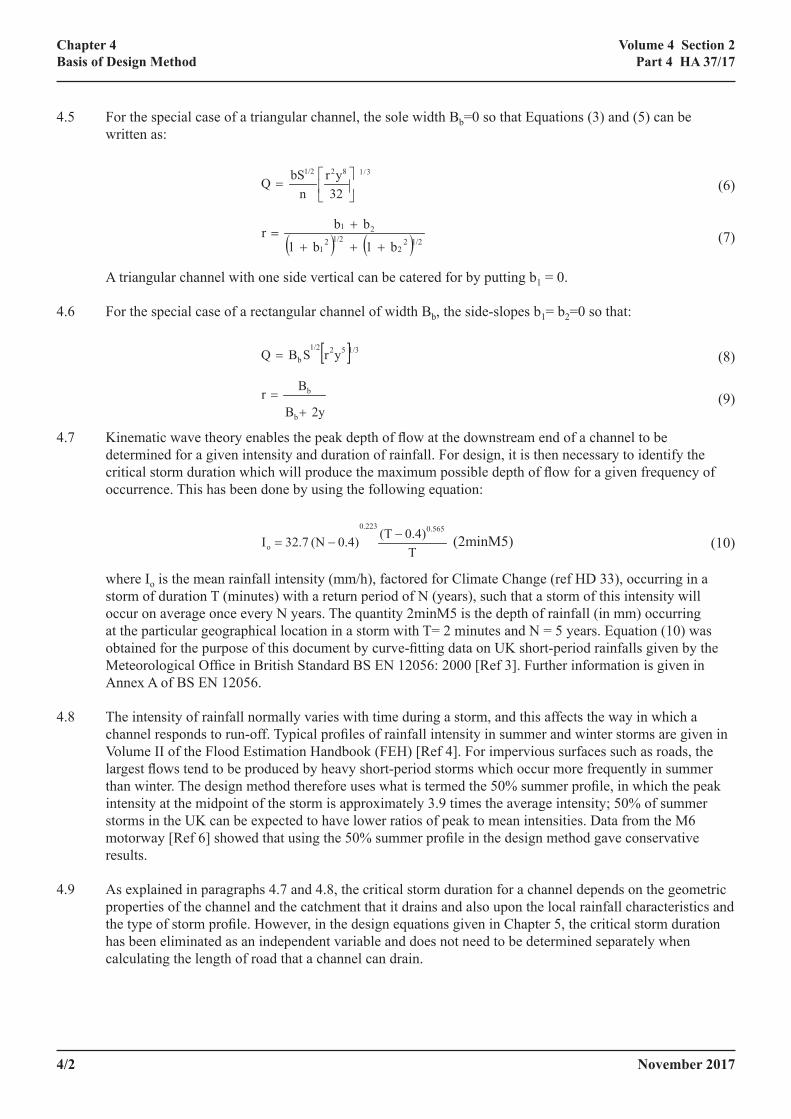
4.5 For the special case of a triangular channel, the sole width Bb=0 so that Equations (3) and (5) can be written as:

n

S AR Q1/22/3

=

R = A / P

( )( )

++

= 522

b

5b

1/2

yrbyB32by2B

nSQ

3/1

b = b1 + b2

( )

( ) ( )[ ]yb1b1B

ybbBr1/22

21/22

1b

21b

++++

++=

=

32yr

nbSQ

821/2 3/1

( ) ( )1/222

1/221

21

b1b1

bbr+++

+=

(6)

n

S AR Q1/22/3

=

R = A / P

( )( )

++

= 522

b

5b

1/2

yrbyB32by2B

nSQ

3/1

b = b1 + b2

( )

( ) ( )[ ]yb1b1B

ybbBr1/22

21/22

1b

21b

++++

++=

=

32yr

nbSQ

821/2 3/1

( ) ( )1/222

1/221

21

b1b1

bbr+++

+=

(7)

A triangular channel with one side vertical can be catered for by putting b1 = 0.

4.6 For the special case of a rectangular channel of width Bb, the side-slopes b1= b2=0 so that:

[ ]1/3521/2b yrSBQ =

2yB

Brb

b

+=

T0.4)(T0.4)(N 32.7I

0.5650.223

o−

−= (2minM5)

(8) [ ]1/3521/2

b yrSBQ =

2yB

Brb

b

+=

T0.4)(T0.4)(N 32.7I

0.5650.223

o−

−= (2minM5)

(9)

4.7 Kinematic wave theory enables the peak depth of flow at the downstream end of a channel to be determined for a given intensity and duration of rainfall. For design, it is then necessary to identify the critical storm duration which will produce the maximum possible depth of flow for a given frequency of occurrence. This has been done by using the following equation:

[ ]1/3521/2b yrSBQ =

2yB

Brb

b

+=

T0.4)(T0.4)(N 32.7I

0.5650.223

o−

−= (2minM5)

(10)

where Io is the mean rainfall intensity (mm/h), factored for Climate Change (ref HD 33), occurring in a storm of duration T (minutes) with a return period of N (years), such that a storm of this intensity will occur on average once every N years. The quantity 2minM5 is the depth of rainfall (in mm) occurring at the particular geographical location in a storm with T= 2 minutes and N = 5 years. Equation (10) was obtained for the purpose of this document by curve-fitting data on UK short-period rainfalls given by the Meteorological Office in British Standard BS EN 12056: 2000 [Ref 3]. Further information is given in Annex A of BS EN 12056.

4.8 The intensity of rainfall normally varies with time during a storm, and this affects the way in which a channel responds to run-off. Typical profiles of rainfall intensity in summer and winter storms are given in Volume II of the Flood Estimation Handbook (FEH) [Ref 4]. For impervious surfaces such as roads, the largest flows tend to be produced by heavy short-period storms which occur more frequently in summer than winter. The design method therefore uses what is termed the 50% summer profile, in which the peak intensity at the midpoint of the storm is approximately 3.9 times the average intensity; 50% of summer storms in the UK can be expected to have lower ratios of peak to mean intensities. Data from the M6 motorway [Ref 6] showed that using the 50% summer profile in the design method gave conservative results.

4.9 As explained in paragraphs 4.7 and 4.8, the critical storm duration for a channel depends on the geometric properties of the channel and the catchment that it drains and also upon the local rainfall characteristics and the type of storm profile. However, in the design equations given in Chapter 5, the critical storm duration has been eliminated as an independent variable and does not need to be determined separately when calculating the length of road that a channel can drain.

November 2017 5/1

Chapter 5Description of Design Equations


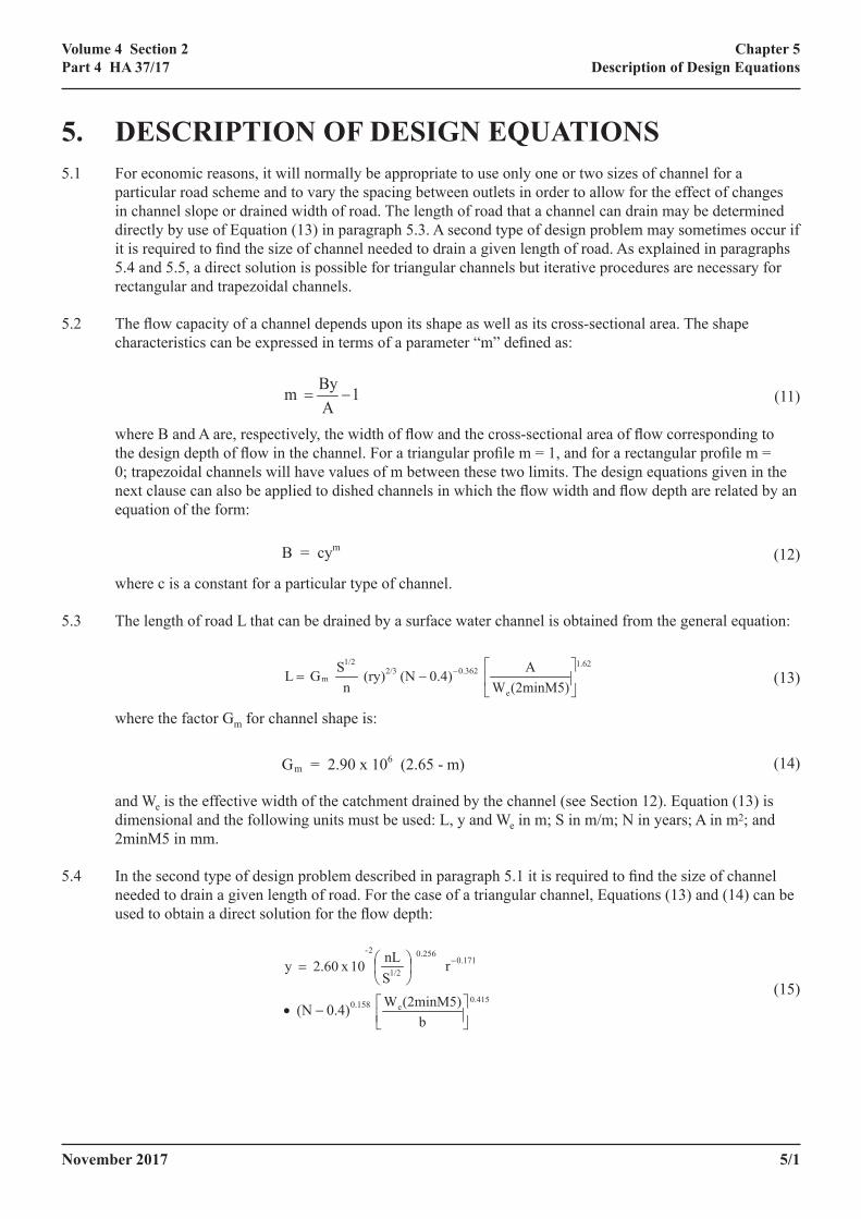
5. DESCRIPTION OF DESIGN EQUATIONS5.1 For economic reasons, it will normally be appropriate to use only one or two sizes of channel for a

particular road scheme and to vary the spacing between outlets in order to allow for the effect of changes in channel slope or drained width of road. The length of road that a channel can drain may be determined directly by use of Equation (13) in paragraph 5.3. A second type of design problem may sometimes occur if it is required to find the size of channel needed to drain a given length of road. As explained in paragraphs 5.4 and 5.5, a direct solution is possible for triangular channels but iterative procedures are necessary for rectangular and trapezoidal channels.

5.2 The flow capacity of a channel depends upon its shape as well as its cross-sectional area. The shape characteristics can be expressed in terms of a parameter “m” defined as:

1ABy m −=

B = cym

0.3622/31/2

m 0.4)(N (ry)n

SG L −−=1.62

e(2minM5)WA

Gm = 2.90 x 106 (2.65 - m)

= 1/2

2-

SnL10x 2.60 y

256.0

171.0r−

0.1580.4)(N −•0.415

e

b(2minM5)W

0.292

b

0.437

1/24-

B2y 1

SnL 10x 2.60 y

+

=

0.1580.4)(N −•0.708

b

e

B(2minM5)W

(11)

where B and A are, respectively, the width of flow and the cross-sectional area of flow corresponding to the design depth of flow in the channel. For a triangular profile m = 1, and for a rectangular profile m = 0; trapezoidal channels will have values of m between these two limits. The design equations given in the next clause can also be applied to dished channels in which the flow width and flow depth are related by an equation of the form:

1ABy m −=

B = cym

0.3622/31/2

m 0.4)(N (ry)n

SG L −−=1.62

e(2minM5)WA

Gm = 2.90 x 106 (2.65 - m)

= 1/2

2-

SnL10x 2.60 y

256.0

171.0r−

0.1580.4)(N −•0.415

e

b(2minM5)W

0.292

b

0.437

1/24-

B2y 1

SnL 10x 2.60 y

+

=

0.1580.4)(N −•0.708

b

e

B(2minM5)W

(12)

where c is a constant for a particular type of channel.

5.3 The length of road L that can be drained by a surface water channel is obtained from the general equation:

1ABy m −=

B = cym

0.3622/31/2

m 0.4)(N (ry)n

SG L −−=1.62

e(2minM5)WA

Gm = 2.90 x 106 (2.65 - m)

= 1/2

2-

SnL10x 2.60 y

256.0

171.0r−

0.1580.4)(N −•0.415

e

b(2minM5)W

0.292

b

0.437

1/24-

B2y 1

SnL 10x 2.60 y

+

=

0.1580.4)(N −•0.708

b

e

B(2minM5)W

(13)

where the factor Gm for channel shape is:

1ABy m −=

B = cym

0.3622/31/2

m 0.4)(N (ry)n

SG L −−=1.62

e(2minM5)WA

Gm = 2.90 x 106 (2.65 - m)

= 1/2

2-

SnL10x 2.60 y

256.0

171.0r−

0.1580.4)(N −•0.415

e

b(2minM5)W

0.292

b

0.437

1/24-

B2y 1

SnL 10x 2.60 y

+

=

0.1580.4)(N −•0.708

b

e

B(2minM5)W

(14)

and We is the effective width of the catchment drained by the channel (see Section 12). Equation (13) is dimensional and the following units must be used: L, y and We in m; S in m/m; N in years; A in m2; and 2minM5 in mm.

5.4 In the second type of design problem described in paragraph 5.1 it is required to find the size of channel needed to drain a given length of road. For the case of a triangular channel, Equations (13) and (14) can be used to obtain a direct solution for the flow depth:

1ABy m −=

B = cym

0.3622/31/2

m 0.4)(N (ry)n

SG L −−=1.62

e(2minM5)WA

Gm = 2.90 x 106 (2.65 - m)

= 1/2

2-

SnL10x 2.60 y

256.0

171.0r−

0.1580.4)(N −•0.415

e

b(2minM5)W

0.292

b

0.437

1/24-

B2y 1

SnL 10x 2.60 y

+

=

0.1580.4)(N −•0.708

b

e

B(2minM5)W

(15)

5/2 November 2017

Chapter 5Description of Design Equations


where the effective cross-fall b and the hydraulic-radius factor r are given by Equations (4) and (7) respectively. For the situation of a rectangular channel of width Bb, the corresponding result is:

1ABy m −=

B = cym

0.3622/31/2

m 0.4)(N (ry)n

SG L −−=1.62

e(2minM5)WA

Gm = 2.90 x 106 (2.65 - m)

= 1/2

2-

SnL10x 2.60 y

256.0

171.0r−

0.1580.4)(N −•0.415

e

b(2minM5)W

0.292

b

0.437

1/24-

B2y 1

SnL 10x 2.60 y

+

=

0.1580.4)(N −•0.708

b

e

B(2minM5)W

(16)

In this case, the unknown flow depth y appears on both sides of the equation so a small amount of iteration is needed to find the solution. The units for the quantities in Equations (15) and (16) must be as specified in paragraph 5.3.

5.5 No general equation for directly determining the flow depth y in trapezoidal channels can be obtained because different solutions are possible depending upon the particular values of base width and side-slope chosen. The following design procedure is therefore recommended.

(a) Make an initial estimate of the size and shape of channel needed.

(b) Calculate the flow area A and the hydraulic-radius factor r (from Equation (5)).

(c) Determine the values of m from Equation (11) and Gm from Equation (14).

(d) Calculate from Equation (13) the length L of road that can be drained and compare with the required length.

(e) Revise the channel geometry and repeat steps (a) to (d) until the required drainage length is achieved.

5.6 If it is necessary to determine the critical storm duration that produces the design flow conditions in a channel, a method of estimating the duration is given in Annex A.

5.7 Information on how to calculate or choose suitable values for the various parameters in Equations (13), (15) and (16) are given in Chapters 6 to 14.

November 2017 6/1

Chapter 6Storm Return Period


6. STORM RETURN PERIOD6.1 The degree of security against flooding that should be provided by a surface drainage channel needs to be

decided on a case-by-case basis.

6.2 On critical lengths of road, it may be necessary to design channels for storms of higher return period than normal in order to reduce the risk of overflowing. Examples are lengths in which a change in superelevation from one side of the road to the other causes the cross-fall to be locally zero; flooding at such a point might spread across the full width of the road. A higher standard of design may also be appropriate for sections draining to longitudinal sag points where it is important to prevent ponding.

6.3 In the absence of special factors of the type described in paragraph 6.2, it will normally be appropriate for a channel in the verge to be designed to just flow full for a storm with a return period of N = 1 year. The cross section profile shown in the HCD (MCHW 3) and HA 39 (DMRB 4.2) can have the outer edge of a verge channel (farthest from the carriageway) set higher than the inner edge, as shown in Figure 3.1. This allows some surcharging to occur on to the adjacent hardstrip or hardshoulder during less frequent storm events. The maximum permissible widths of flooding are stated in HD33 as 1.0m for all-purpose roads and 1.5m for motorways. As an example, a 1.0m width of flooding on a road with a cross-fall of 1:40 can be allowed by constructing the outer edge of the channel so that it is 25mm higher than the inner edge. Larger flows will cause the channel to overflow into the verge rather than to encroach farther on to the carriageway. Unless there are special factors, it will normally be appropriate to check that a surcharged channel is able to cater for a storm with a return period of N = 5 years without overflowing.

6.4 Channels in the central reserve may need to be designed to a higher standard than those in the verge because it is important to prevent water from encroaching on to the adjacent lane or from overflowing on to the opposite carriageway. HA 39 (DMRB 4.2) contains the geometric requirements in order to prevent such occurrences. If no surcharging of a channel in the central reserve is permissible, the channel should be designed to flow just full for a storm with a return period of N = 5 years (in the absence of other special factors such as those described in paragraph 6.2).

6.5 If the cross-sectional profile in the central reserve does safely permit some surcharging, then the normal design requirements should be similar to those for verge channels: ie, N = 1 year for the channel just flowing full; and N = 5 years for the channel with the permitted amount of surcharging.

6.6 The standard of performance appropriate for critical sections of road (see paragraph 6.2) will depend upon the particular circumstances but design storm return periods of N = 10 years or N = 20 years may be suitable choices.

6/2 November 2017

Chapter 6Storm Return Period


November 2017 7/1

Chapter 7Geographical Location


7. GEOGRAPHICAL LOCATION7.1 The effect of geographical location on rainfall characteristics is taken into account in Equation (10) by

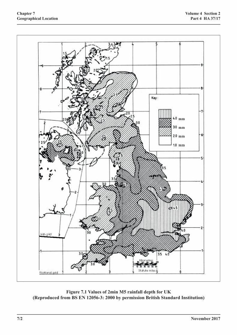
means of the value of 2minM5 – the rainfall depth (in mm) occurring in a storm event with a duration of T = 2 minutes and a return period of N = 5 years. The value of 2minM5 appropriate for any particular road scheme in the UK is obtained from Figure 7.1 (taken from BS EN 12056-3: 2000, Ref 3). This value is then used in the design Equations (13), (15) or (16) as appropriate. The rainfall intensity used in the calculations should be increased to allow for the effects of climate change, by the percentage stated in HD33.

7.2 It should be noted from Figure 7.1 that the most severe rainfall conditions are to be expected in East Anglia and the South-East of England. Although these areas have much lower values of average annual rainfall than parts of Wales, Scotland and the North-West of England, they experience heavier and more frequent short-duration storms, of the kind typically associated with summer thunderstorms.

7/2 November 2017

Chapter 7Geographical Location


Figure 7.1 Values of 2min M5 rainfall depth for UK

(Reproduced from BS EN 12056-3: 2000 by permission British Standard Institution)

November 2017 8/1

Chapter 8Channel Geometry


8. CHANNEL GEOMETRY8.1 The design equations (13), (15) and (16) are valid for all types of triangular, rectangular or trapezoidal

channel provided the cross-sectional shape factors b1, b2 and Bb (as appropriate) do not vary with the depth of flow or with distance along the drainage length.

8.2 Limits on the permissible depth and side-slopes for surface water channels that may be subject to traffic are given in paragraph 3.1. A trapezoidal channel provides a higher flow capacity than a triangular channel with the same depth and side-slopes and will therefore enable longer lengths of road to be drained between outlets. If a channel is protected or removed far enough from traffic, larger depths or steeper side-slopes can be used; the occurrence of the flow depth y in Equation (13) shows that a relatively deeper channel is more efficient hydraulically than a shallower channel of the same cross-sectional area.

8.3 The base sections of trapezoidal or rectangular channels should be given a 1:40 cross-fall away from the carriageway (see Figure 2.1) so as to provide self-cleansing characteristics that are similar to those of conventional kerbed channels. The effect of the 1:40 cross-fall on flow capacity is very small and can be neglected; the value of y used in Equations (11), (13) and (16) should be the flow depth measured from the centreline of the channel invert.

8.4 Figure 3.1 defines the flow depths that may need to be considered when designing a surface water channel. The depth y1 from the lower inner edge of the channel to the centreline of the invert corresponds to the channel full capacity and is termed the “design flow depth”. If water is permitted to encroach on to the adjacent hardstrip or hardshoulder during rarer storms, the “surcharged flow depth” y3 is the depth from the outer edge of the channel to the centreline of the invert. There should, if possible, be no step between the inner edge of the channel and the top edge of the carriageway. However, if one is formed, it may be necessary in the calculations to take account of the depth y2 between the top edge of the carriageway and the centreline of the channel invert. In cases where porous asphalt surfacing is used in conjunction with road-edge channels, a step will normally be necessary to allow water to drain from the permeable layer; the vertical distance between the top of the porous asphalt layer and the invert of the channel should not exceed 150mm.

8.5 As described in Chapter 6, surface water channels should be designed to provide security against flooding. As an example, a verge channel might typically be sized so that the design flow depth y1 provides sufficient flow capacity for storms with a return period of N = 1 year. In some instances it may be desirable that the channel is able to cater for storms of N = 5 years without exceeding the surcharged flow depth y3. If the second criterion was not satisfied, the size of the channel would need to be increased or the distance between outlets reduced. If no surcharging was permitted (eg, for a channel in the central reserve), it might be specified that the design flow depth y1 should provide sufficient capacity for storm return periods of N = 5 years. Further guidance on the choice of suitable design criteria is given in Chapter 6.

8.6 If a channel is permitted to surcharge, the cross-sectional shape of the flow area becomes more complex and does not comply with the assumptions given in paragraph 8.1. An approximate method of determining the drainage capacity of surcharged channels is given in Chapter 13.

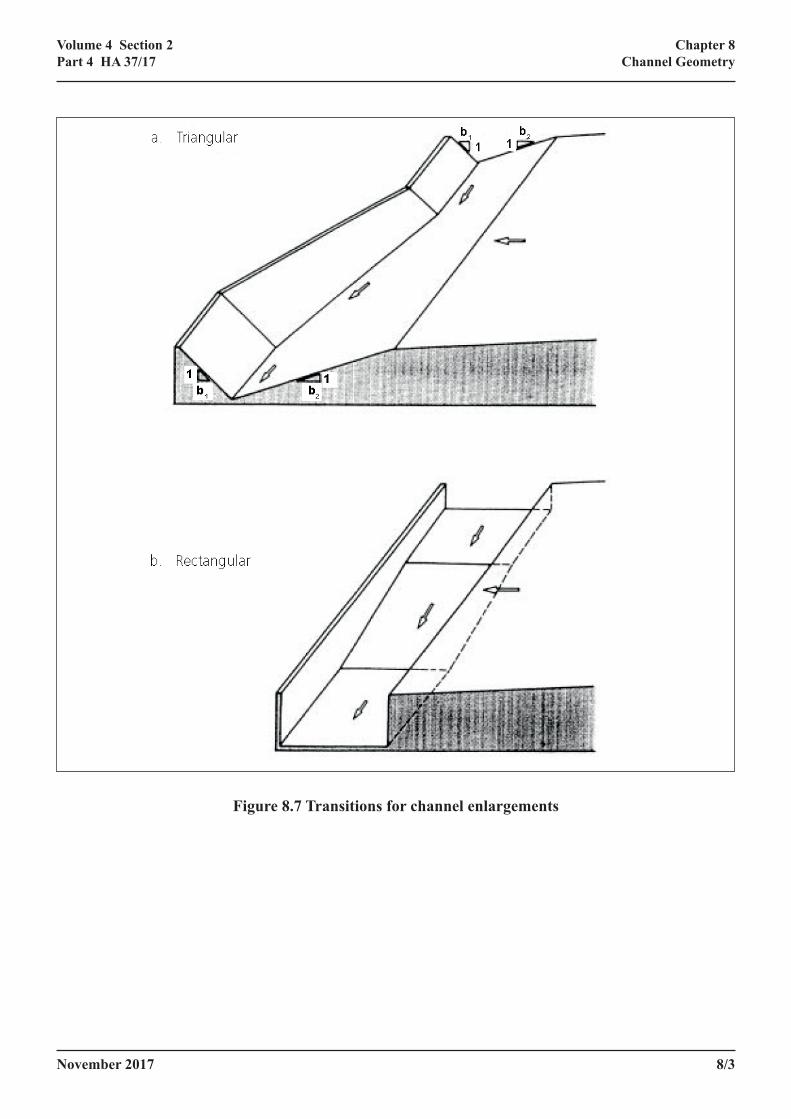
8.7 In some situations it may be wished to increase the size of a channel part way along a drainage length. In the case of a triangular profile, it is possible to deepen the channel without altering the cross-falls b1 and b2, and similarly a rectangular channel can be deepened while keeping the width Bb constant; examples of suitable transitions are shown in Figure 8.7. The design equations (13), (15) and (16) can be applied to such cases without approximation. The flow capacity of the smaller, upstream channel should be checked to ensure that it is sufficient to drain the length of road upstream of the transition point; the capacity of the larger, downstream channel should be similarly checked using the overall length of road draining to the outlet.

8/2 November 2017



8.8 If a trapezoidal channel is enlarged part way along a drainage length, it is not possible to keep all the shape factors b1, b2 and Bb constant. The capacities of the two parts of the channel should be checked in the way described in paragraph 8.7, but the result for the downstream length may be less accurate because the assumption of constant shape is not satisfied. For this reason, it is recommended that the downstream channel should be designed assuming a drainage length 5% greater than the actual length draining to the outlet.

8.9 Transitions of the type shown in Figure 8.7 should be gradual in order to minimize energy losses. If the invert is lowered, the length of the transition should not be less than 15 times the change in depth. Similarly, the side of a channel should not diverge outwards from the longitudinal centreline at an angle greater than 1:3 in plan.

8.10 Fixed obstructions in a drainage channel, such as a longitudinal line of posts for a road restraint barrier, will reduce its flow capacity. In order to prevent excessive local disturbance of the flow, no more than 15% of the cross- sectional area of the flow should be blocked by an obstruction if it is located within the downstream half of a drainage length; in the upstream half the blockage should not be more than 25% of the cross-sectional area of the flow. The energy losses produced by a longitudinal line of posts can be taken into account by using a higher value of the Manning resistance coefficient n, as described in paragraph 11.2. Allowance need not normally be made for one or two isolated posts in a particular drainage length.

November 2017 8/3



Figure 8.7 Transitions for channel enlargements

8/4 November 2017



November 2017 9/1

Chapter 9Channel Gradient


9. CHANNEL GRADIENT9.1 The longitudinal gradient S of a channel is defined as the vertical fall per unit distance measured along the

channel. A channel will normally have the same longitudinal gradient as the adjacent carriageway, but this is not a condition for use of the design method.

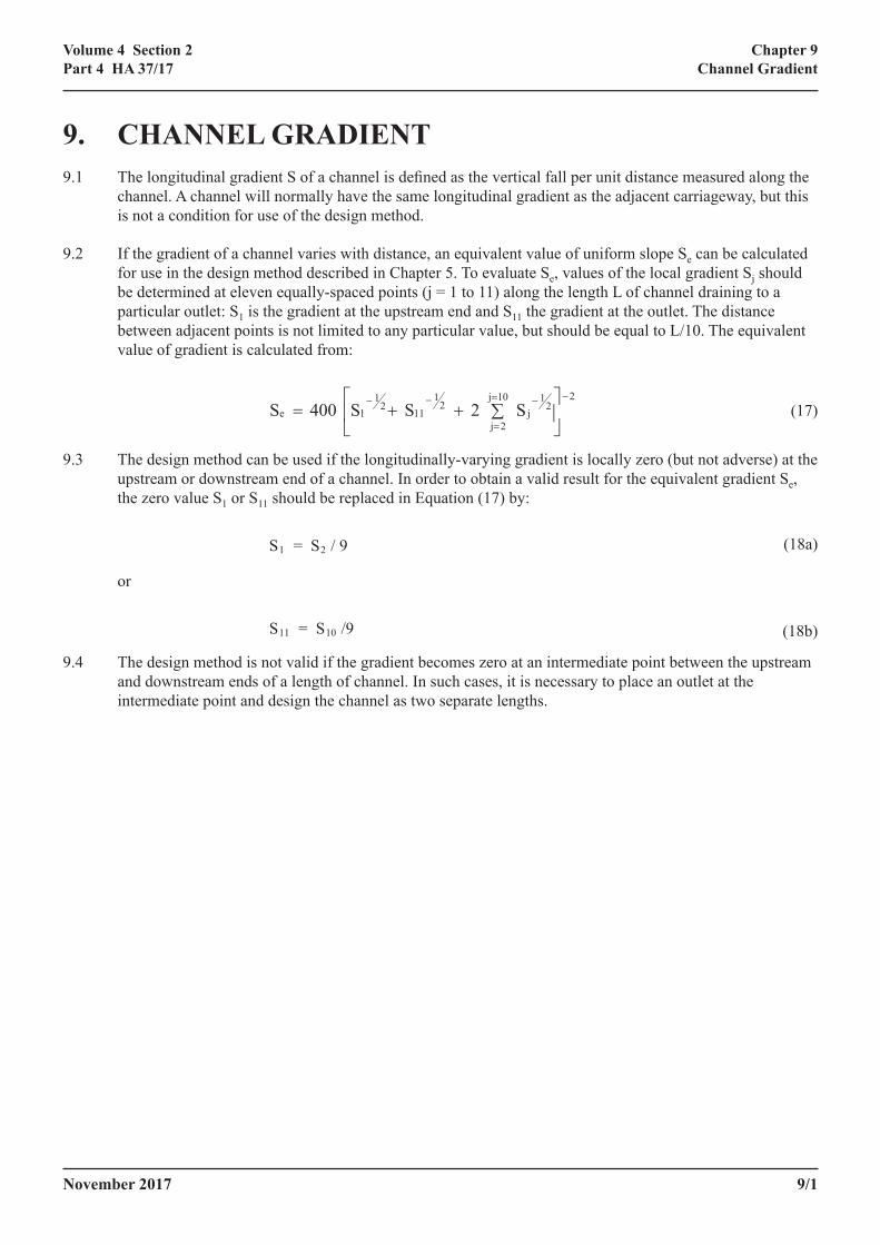
9.2 If the gradient of a channel varies with distance, an equivalent value of uniform slope Se can be calculated for use in the design method described in Chapter 5. To evaluate Se, values of the local gradient Sj should be determined at eleven equally-spaced points (j = 1 to 11) along the length L of channel draining to a particular outlet: S1 is the gradient at the upstream end and S11 the gradient at the outlet. The distance between adjacent points is not limited to any particular value, but should be equal to L/10. The equivalent value of gradient is calculated from:

22

1j

10j

2j

21

112

11e S2SS400S

−−=

=

−−

∑++=

S1 = S2 / 9

S11 = S10 /9

(17)

9.3 The design method can be used if the longitudinally-varying gradient is locally zero (but not adverse) at the upstream or downstream end of a channel. In order to obtain a valid result for the equivalent gradient Se, the zero value S1 or S11 should be replaced in Equation (17) by:

22

1j

10j

2j

21

112

11e S2SS400S

−−=

=

−−

∑++=

S1 = S2 / 9

S11 = S10 /9

(18a)

or

22

1j

10j

2j

21

112

11e S2SS400S

−−=

=

−−

∑++=

S1 = S2 / 9

S11 = S10 /9

(18b)

9.4 The design method is not valid if the gradient becomes zero at an intermediate point between the upstream and downstream ends of a length of channel. In such cases, it is necessary to place an outlet at the intermediate point and design the channel as two separate lengths.

9/2 November 2017

Chapter 9Channel Gradient


November 2017 10/1

Chapter 10Drainage Lengths


10. DRAINAGE LENGTHS10.1 The drainage length L is the distance along a channel between two adjacent outlets on a continuous slope,

or the distance between a point of zero slope and the downstream outlet.

10.2 Surface water channels can be used most effectively if their layout is considered at an early stage in the design of a road scheme. Where possible, horizontal and vertical alignments should be chosen so that suitable drainage lengths can be defined taking into account the location of outlets discharging to natural watercourses.

10.3 If the drainage length to a natural watercourse requires too large a channel capacity, intermediate outlets should be used to remove water from the road-edge channel. The flow from the outlets may be conveyed to a suitable discharge point by carrier pipes or an open ditch.

10/2 November 2017

Chapter 10Drainage Lengths


November 2017 11/1

Chapter 11Channel Roughness


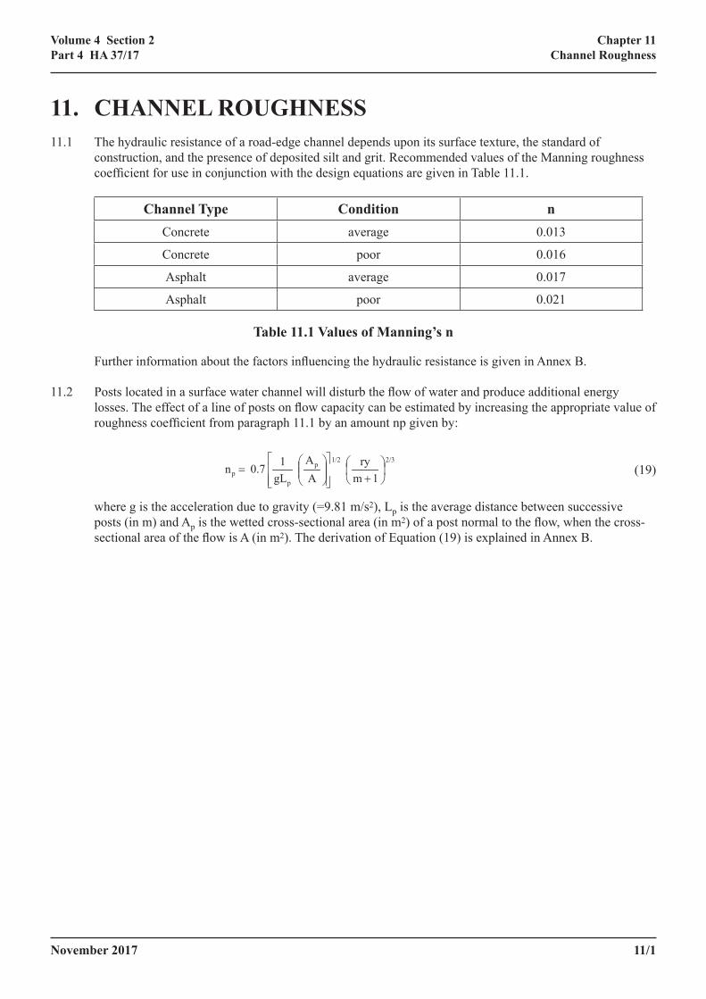
11. CHANNEL ROUGHNESS11.1 The hydraulic resistance of a road-edge channel depends upon its surface texture, the standard of

construction, and the presence of deposited silt and grit. Recommended values of the Manning roughness coefficient for use in conjunction with the design equations are given in Table 11.1.

Channel Type Condition nConcrete average 0.013

Concrete poor 0.016

Asphalt average 0.017

Asphalt poor 0.021

Table 11.1 Values of Manning’s n

Further information about the factors influencing the hydraulic resistance is given in Annex B.

11.2 Posts located in a surface water channel will disturb the flow of water and produce additional energy losses. The effect of a line of posts on flow capacity can be estimated by increasing the appropriate value of roughness coefficient from paragraph 11.1 by an amount np given by:

2/31/2

p

pp 1m

ry AA

gL

1 0.7 n

+

=

(19)

where g is the acceleration due to gravity (=9.81 m/s2), Lp is the average distance between successive posts (in m) and Ap is the wetted cross-sectional area (in m2) of a post normal to the flow, when the cross-sectional area of the flow is A (in m2). The derivation of Equation (19) is explained in Annex B.

11/2 November 2017

Chapter 11Channel Roughness


November 2017 12/1

Chapter 12Catchment Width


12. CATCHMENT WIDTH12.1 The effective catchment width We is equal to the width of the carriageway drained, plus the width of the

channel and any other impermeable surface draining to the channel, plus an allowance (if appropriate) for runoff from a cutting.

12.2 The design method assumes that We does not vary along a particular drainage length. However, minor local variations can be allowed for by using an average width, calculated by dividing the total effective area draining to an outlet by the drainage length L.

12.3 It is assumed that 100% run-off occurs from concrete and black-top surfaces during design storms.

12.4 Surface channels may be used to collect run-off from cuttings as well as from roads. The amount of runoff from a cutting depends upon many factors including its height, slope, soil type and antecedent wetness, and also upon the quantity of rainfall and the direction of the wind.

12.5 Information on the additional run-off contributed by cuttings is very limited. In the absence of suitable field data, the effective width We of a catchment should be calculated from the formula:

We = W + α C

(20)

where W is the width of the impermeable part of the catchment (m), a is the run-off coefficient for the cutting, and is the average plan width of the cutting (m) drained by the length of channel being considered. Details of the derivation of Equation (20) are given in Annex C.

12.6 Suitable values of the run-off coefficient a can be estimated from Table 12.6.1. These figures contain some allowance for the relative steepness of road cuttings, which may result in more run-off than from equivalent natural catchments. For design purposes it is assumed that the antecedent wetness of the cutting is dependent upon the average annual rainfall at the site. Appropriate choices of antecedent wetness for Northern Ireland, Scotland, Wales and English Counties are given in Table 12.6.2.

Soil Type Antecedent Wetness α

High permeability low

medium

high

0.07

0.11

0.13

Medium permeability low

medium

high

0.11

0.16

0.20

Low permeability low

medium

high

0.14

0.21

0.26

Table12.6.1Run-offcoefficientsforcuttings

12/2 November 2017

Chapter 12Catchment Width


Low Medium HighBedfordshireBuckinghamshireCambridgeshireEssexGreater LondonHertfordshireNorfolkRutlandSuffolk

BerkshireClevelandDerbyshireDurhamEast SussexHampshireHereford & WorcesterHumbersideIsle of WightKentLeicestershireLincolnshireNorth YorkshireNorthamptonshireNorthumberlandNottinghamshireOxfordshireShropshireSouth YorkshireStaffordshireSurreyTyne & WearWarwickshireWest SussexWest Yorkshire

Northern IrelandScotlandWalesAvonCheshireCornwallCumbriaDevonDorsetGloucestershireGreater ManchesterLancashireMerseysideSomersetWiltshire

Table 12.6.2 Antecedent wetness categories

The basis of the data in Tables 12.6.1 and 12.6.2 is explained in Annex C.

November 2017 13/1

Chapter 13Surcharged Channels


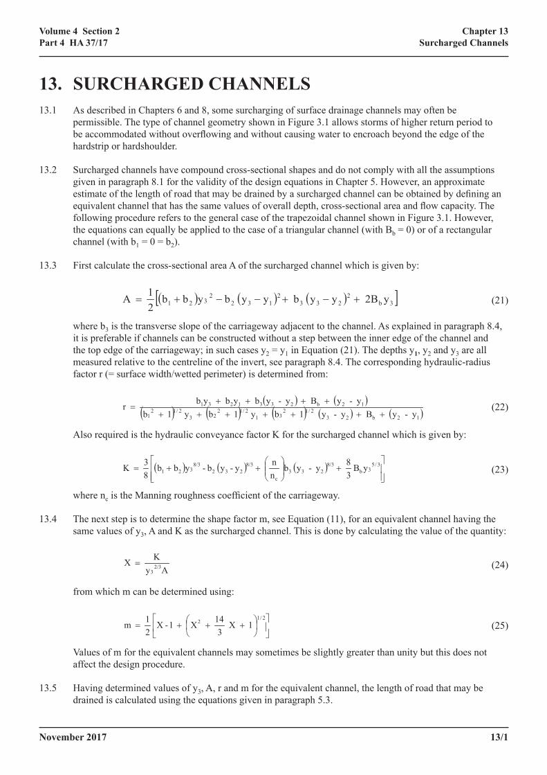
13. SURCHARGED CHANNELS13.1 As described in Chapters 6 and 8, some surcharging of surface drainage channels may often be

permissible. The type of channel geometry shown in Figure 3.1 allows storms of higher return period to be accommodated without overflowing and without causing water to encroach beyond the edge of the hardstrip or hardshoulder.

13.2 Surcharged channels have compound cross-sectional shapes and do not comply with all the assumptions given in paragraph 8.1 for the validity of the design equations in Chapter 5. However, an approximate estimate of the length of road that may be drained by a surcharged channel can be obtained by defining an equivalent channel that has the same values of overall depth, cross-sectional area and flow capacity. The following procedure refers to the general case of the trapezoidal channel shown in Figure 3.1. However, the equations can equally be applied to the case of a triangular channel (with Bb = 0) or of a rectangular channel (with b1 = 0 = b2).

13.3 First calculate the cross-sectional area A of the surcharged channel which is given by:

( ) ( ) ( )[ ]3b2

2332

1322

321 y2B y y b y y b yb b 21 A +−+−−+=

( ) ( )( ) ( ) ( ) ( ) ( )12b23

2/1231

2/1223

2/121

12b2331231

y- y B y- y 1 b y1 b y1 b y- y B y- yb yb yb r

+++++++++++

=

( ) ( ) ( )

+

++= 3/5

3b8/3

233c

8/3232

8/3321 y B

38 y- y b

nn y- y b - yb b

83 K

Ay

K X 2/33

=

+++=

2/12 1 X

314 X 1 - X

21 m

(21)

where b3 is the transverse slope of the carriageway adjacent to the channel. As explained in paragraph 8.4, it is preferable if channels can be constructed without a step between the inner edge of the channel and the top edge of the carriageway; in such cases y2 = y1 in Equation (21). The depths y1, y2 and y3 are all measured relative to the centreline of the invert, see paragraph 8.4. The corresponding hydraulic-radius factor r (= surface width/wetted perimeter) is determined from:

( ) ( ) ( )[ ]3b2

2332

1322

321 y2B y y b y y b yb b 21 A +−+−−+=

( ) ( )( ) ( ) ( ) ( ) ( )12b23

2/1231

2/1223

2/121

12b2331231


+++++++++++

=

( ) ( ) ( )

+

++= 3/5

3b8/3

233c

8/3232

8/3321 y B

38 y- y b

nn y- y b - yb b

83 K

Ay

K X 2/33

=

+++=

2/12 1 X

314 X 1 - X

21 m

(22)

Also required is the hydraulic conveyance factor K for the surcharged channel which is given by:

( ) ( ) ( )[ ]3b2

2332

1322

321 y2B y y b y y b yb b 21 A +−+−−+=

( ) ( )( ) ( ) ( ) ( ) ( )12b23

2/1231

2/1223

2/121

12b2331231


+++++++++++

=

( ) ( ) ( )

+

++= 3/5

3b8/3

233c

8/3232

8/3321 y B

38 y- y b

nn y- y b - yb b

83 K

Ay

K X 2/33

=

+++=

2/12 1 X

314 X 1 - X

21 m

(23)

where nc is the Manning roughness coefficient of the carriageway.

13.4 The next step is to determine the shape factor m, see Equation (11), for an equivalent channel having the same values of y3, A and K as the surcharged channel. This is done by calculating the value of the quantity:

( ) ( ) ( )[ ]3b2

2332

1322

321 y2B y y b y y b yb b 21 A +−+−−+=

( ) ( )( ) ( ) ( ) ( ) ( )12b23

2/1231

2/1223

2/121

12b2331231


+++++++++++

=

( ) ( ) ( )

+

++= 3/5

3b8/3

233c

8/3232

8/3321 y B

38 y- y b

nn y- y b - yb b

83 K

Ay

K X 2/33

=

+++=

2/12 1 X

314 X 1 - X

21 m

(24)

from which m can be determined using:

( ) ( ) ( )[ ]3b2

2332

1322

321 y2B y y b y y b yb b 21 A +−+−−+=

( ) ( )( ) ( ) ( ) ( ) ( )12b23

2/1231

2/1223

2/121

12b2331231


+++++++++++

=

( ) ( ) ( )

+

++= 3/5

3b8/3

233c

8/3232

8/3321 y B

38 y- y b

nn y- y b - yb b

83 K

Ay

K X 2/33

=

+++=

2/12 1 X

314 X 1 - X

21 m

(25)

Values of m for the equivalent channels may sometimes be slightly greater than unity but this does not affect the design procedure.

13.5 Having determined values of y3, A, r and m for the equivalent channel, the length of road that may be drained is calculated using the equations given in paragraph 5.3.

13/2 November 2017

Chapter 13Surcharged Channels


November 2017 14/1

Chapter 14By-Passing at Outlets


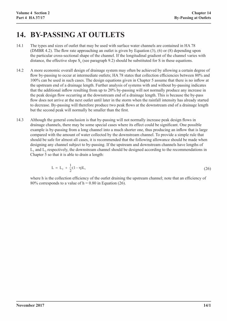
14. BY-PASSING AT OUTLETS14.1 The types and sizes of outlet that may be used with surface water channels are contained in HA 78

(DMBR 4.2). The flow rate approaching an outlet is given by Equation (3), (6) or (8) depending upon the particular cross-sectional shape of the channel. If the longitudinal gradient of the channel varies with distance, the effective slope Se (see paragraph 9.2) should be substituted for S in these equations.

14.2 A more economic overall design of drainage system may often be achieved by allowing a certain degree of flow by-passing to occur at intermediate outlets; HA 78 states that collection efficiencies between 80% and 100% can be used in such cases. The design equations given in Chapter 5 assume that there is no inflow at the upstream end of a drainage length. Further analysis of systems with and without by-passing indicates that the additional inflow resulting from up to 20% by-passing will not normally produce any increase in the peak design flow occurring at the downstream end of a drainage length. This is because the by-pass flow does not arrive at the next outlet until later in the storm when the rainfall intensity has already started to decrease. By-passing will therefore produce two peak flows at the downstream end of a drainage length but the second peak will normally be smaller than the first.

14.3 Although the general conclusion is that by-passing will not normally increase peak design flows in drainage channels, there may be some special cases where its effect could be significant. One possible example is by-passing from a long channel into a much shorter one, thus producing an inflow that is large compared with the amount of water collected by the downstream channel. To provide a simple rule that should be safe for almost all cases, it is recommended that the following allowance should be made when designing any channel subject to by-passing. If the upstream and downstream channels have lengths of L1 and L2 respectively, the downstream channel should be designed according to the recommendations in Chapter 5 so that it is able to drain a length:

12 )L (121 L L η−+=

(26)

where h is the collection efficiency of the outlet draining the upstream channel; note that an efficiency of 80% corresponds to a value of h = 0.80 in Equation (26).

14/2 November 2017

Chapter 14By-Passing at Outlets


November 2017 15/1

Chapter 15Construction Tolerances


15. CONSTRUCTION TOLERANCES15.1 The effect of allowable construction tolerances on the capacity of a channel should be considered in design.

As an approximate guide, flow capacity will be within ±5% of the design capacity if the local channel gradient is within ±10% or the depth of the channel within ±2% of the required values. In general, the design capacity of the channel should be determined for the combination of tolerances that give minimum channel capacity. Adherence to tolerances is most important at the downstream ends of drainage lengths where the flows are greatest.

15/2 November 2017

Chapter 15Construction Tolerances


November 2017 16/1

Chapter 16Worked Examples


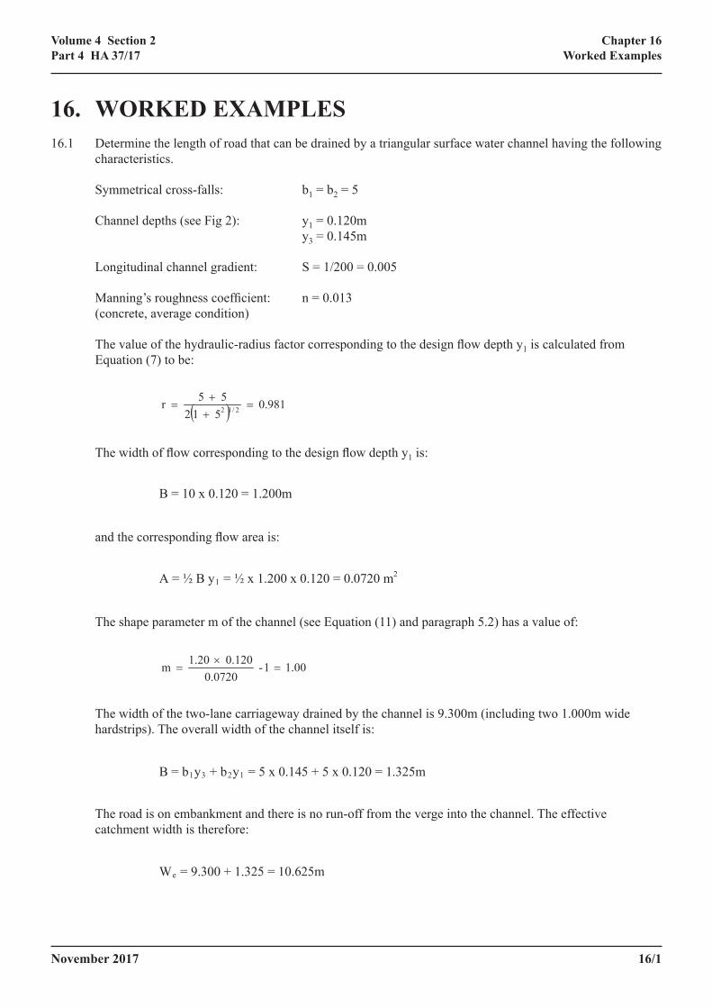
16. WORKED EXAMPLES16.1 Determine the length of road that can be drained by a triangular surface water channel having the following

characteristics.

Symmetrical cross-falls: b1 = b2 = 5

Channel depths (see Fig 2): y1 = 0.120m y3 = 0.145m

Longitudinal channel gradient: S = 1/200 = 0.005

Manning’s roughness coefficient: n = 0.013 (concrete, average condition)

The value of the hydraulic-radius factor corresponding to the design flow depth y1 is calculated from Equation (7) to be:

( ) 0.981 5 12

5 5 r 2/12 =++

=

B = 10 x 0.120 = 1.200m

A = ½ B y1 = ½ x 1.200 x 0.120 = 0.0720 m2

1.00 1- 0.0720

0.120 1.20 m =×

=

B = b1y3 + b2y1 = 5 x 0.145 + 5 x 0.120 = 1.325m

We = 9.300 + 1.325 = 10.625m

2minM5 = 4.0mm

N = 1 year

The width of flow corresponding to the design flow depth y1 is: ( ) 0.981

5 125 5 r 2/12 =

++

=

B = 10 x 0.120 = 1.200m

A = ½ B y1 = ½ x 1.200 x 0.120 = 0.0720 m2

1.00 1- 0.0720

0.120 1.20 m =×

=

B = b1y3 + b2y1 = 5 x 0.145 + 5 x 0.120 = 1.325m

We = 9.300 + 1.325 = 10.625m

2minM5 = 4.0mm

N = 1 year

and the corresponding flow area is:

( ) 0.981 5 12

5 5 r 2/12 =++

=

B = 10 x 0.120 = 1.200m

A = ½ B y1 = ½ x 1.200 x 0.120 = 0.0720 m2

1.00 1- 0.0720

0.120 1.20 m =×

=

B = b1y3 + b2y1 = 5 x 0.145 + 5 x 0.120 = 1.325m

We = 9.300 + 1.325 = 10.625m

2minM5 = 4.0mm

N = 1 year

The shape parameter m of the channel (see Equation (11) and paragraph 5.2) has a value of:

( ) 0.981 5 12

5 5 r 2/12 =++

=

B = 10 x 0.120 = 1.200m

A = ½ B y1 = ½ x 1.200 x 0.120 = 0.0720 m2

1.00 1- 0.0720

0.120 1.20 m =×

=

B = b1y3 + b2y1 = 5 x 0.145 + 5 x 0.120 = 1.325m

We = 9.300 + 1.325 = 10.625m

2minM5 = 4.0mm

N = 1 year

The width of the two-lane carriageway drained by the channel is 9.300m (including two 1.000m wide hardstrips). The overall width of the channel itself is:

( ) 0.981 5 12

5 5 r 2/12 =++

=

B = 10 x 0.120 = 1.200m

A = ½ B y1 = ½ x 1.200 x 0.120 = 0.0720 m2

1.00 1- 0.0720

0.120 1.20 m =×

=

B = b1y3 + b2y1 = 5 x 0.145 + 5 x 0.120 = 1.325m

We = 9.300 + 1.325 = 10.625m

2minM5 = 4.0mm

N = 1 year

The road is on embankment and there is no run-off from the verge into the channel. The effective catchment width is therefore:

( ) 0.981 5 12

5 5 r 2/12 =++

=

B = 10 x 0.120 = 1.200m

A = ½ B y1 = ½ x 1.200 x 0.120 = 0.0720 m2

1.00 1- 0.0720

0.120 1.20 m =×

=

B = b1y3 + b2y1 = 5 x 0.145 + 5 x 0.120 = 1.325m

We = 9.300 + 1.325 = 10.625m

2minM5 = 4.0mm

N = 1 year

16/2 November 2017



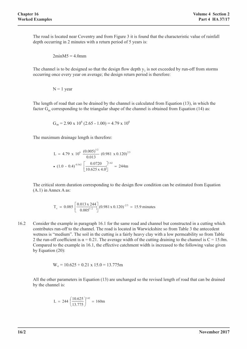
The road is located near Coventry and from Figure 3 it is found that the characteristic value of rainfall depth occurring in 2 minutes with a return period of 5 years is:

( ) 0.981 5 12

5 5 r 2/12 =++

=

B = 10 x 0.120 = 1.200m

A = ½ B y1 = ½ x 1.200 x 0.120 = 0.0720 m2

1.00 1- 0.0720

0.120 1.20 m =×

=

B = b1y3 + b2y1 = 5 x 0.145 + 5 x 0.120 = 1.325m

We = 9.300 + 1.325 = 10.625m

2minM5 = 4.0mm

N = 1 year The channel is to be designed so that the design flow depth y1 is not exceeded by run-off from storms

occurring once every year on average; the design return period is therefore:

( ) 0.981 5 12

5 5 r 2/12 =++

=

B = 10 x 0.120 = 1.200m

A = ½ B y1 = ½ x 1.200 x 0.120 = 0.0720 m2

1.00 1- 0.0720

0.120 1.20 m =×

=

B = b1y3 + b2y1 = 5 x 0.145 + 5 x 0.120 = 1.325m

We = 9.300 + 1.325 = 10.625m

2minM5 = 4.0mm

N = 1 year

The length of road that can be drained by the channel is calculated from Equation (13), in which the factor Gm corresponding to the triangular shape of the channel is obtained from Equation (14) as:

Gm = 2.90 x 106 (2.65 - 1.00) = 4.79 x 106

2/31/2

6 0.120)x (0.981 013.0

(0.005) 10x 4.79 L =

244m 4.0x 10.625

0.0720 0.4) - (1.0 62.1

0.362- =

minutes 15.9 0.120)x (0.981 005.0

244x 0.013 0.085 T 2/3-2/1c =

=

We = 10.625 + 0.21 x 15.0 = 13.775m

160m 13.77510.625 244 L

62.1=

=

( )

0.984 0.150x 5 1 2 0.300

0.150x 5) (5 0.300 r 2

12++

++=

B = 0.300 + 10 x 0.150 = 1.800m

( ) 2221211b 0.158m 0.150x 5) (5 2

1 0.150x 0.300 yb b21 y B A =++=++=

0.71 1- 0.158

0.150 1.800 m =×

=

•

The maximum drainage length is therefore: Gm = 2.90 x 106 (2.65 - 1.00) = 4.79 x 106

2/31/2

6 0.120)x (0.981 013.0

(0.005) 10x 4.79 L =

244m 4.0x 10.625

0.0720 0.4) - (1.0 62.1

0.362- =

minutes 15.9 0.120)x (0.981 005.0

244x 0.013 0.085 T 2/3-2/1c =

=

We = 10.625 + 0.21 x 15.0 = 13.775m

160m 13.77510.625 244 L

62.1=

=

( )

0.984 0.150x 5 1 2 0.300

0.150x 5) (5 0.300 r 2

12++

++=

B = 0.300 + 10 x 0.150 = 1.800m

( ) 2221211b 0.158m 0.150x 5) (5 2

1 0.150x 0.300 yb b21 y B A =++=++=

0.71 1- 0.158

0.150 1.800 m =×

=

•

The critical storm duration corresponding to the design flow condition can be estimated from Equation (A.1) in Annex A as:

Gm = 2.90 x 106 (2.65 - 1.00) = 4.79 x 106

2/31/2

6 0.120)x (0.981 013.0

(0.005) 10x 4.79 L =

244m 4.0x 10.625

0.0720 0.4) - (1.0 62.1

0.362- =

minutes 15.9 0.120)x (0.981 005.0

244x 0.013 0.085 T 2/3-2/1c =

=

We = 10.625 + 0.21 x 15.0 = 13.775m

160m 13.77510.625 244 L

62.1=

=

( )

0.984 0.150x 5 1 2 0.300

0.150x 5) (5 0.300 r 2

12++

++=

B = 0.300 + 10 x 0.150 = 1.800m

( ) 2221211b 0.158m 0.150x 5) (5 2

1 0.150x 0.300 yb b21 y B A =++=++=

0.71 1- 0.158

0.150 1.800 m =×

=

•

16.2 Consider the example in paragraph 16.1 for the same road and channel but constructed in a cutting which contributes run-off to the channel. The road is located in Warwickshire so from Table 3 the antecedent wetness is “medium”. The soil in the cutting is a fairly heavy clay with a low permeability so from Table 2 the run-off coefficient is α = 0.21. The average width of the cutting draining to the channel is C = 15.0m. Compared to the example in 16.1, the effective catchment width is increased to the following value given by Equation (20):

Gm = 2.90 x 106 (2.65 - 1.00) = 4.79 x 106

2/31/2

6 0.120)x (0.981 013.0

(0.005) 10x 4.79 L =

244m 4.0x 10.625

0.0720 0.4) - (1.0 62.1

0.362- =

minutes 15.9 0.120)x (0.981 005.0

244x 0.013 0.085 T 2/3-2/1c =

=

We = 10.625 + 0.21 x 15.0 = 13.775m

160m 13.77510.625 244 L

62.1=

=

( )

0.984 0.150x 5 1 2 0.300

0.150x 5) (5 0.300 r 2

12++

++=

B = 0.300 + 10 x 0.150 = 1.800m

( ) 2221211b 0.158m 0.150x 5) (5 2

1 0.150x 0.300 yb b21 y B A =++=++=

0.71 1- 0.158

0.150 1.800 m =×

=

•

All the other parameters in Equation (13) are unchanged so the revised length of road that can be drained by the channel is:

Gm = 2.90 x 106 (2.65 - 1.00) = 4.79 x 106

2/31/2

6 0.120)x (0.981 013.0

(0.005) 10x 4.79 L =

244m 4.0x 10.625

0.0720 0.4) - (1.0 62.1

0.362- =

minutes 15.9 0.120)x (0.981 005.0

244x 0.013 0.085 T 2/3-2/1c =

=

We = 10.625 + 0.21 x 15.0 = 13.775m

160m 13.77510.625 244 L

62.1=

=

( )

0.984 0.150x 5 1 2 0.300

0.150x 5) (5 0.300 r 2

12++

++=

B = 0.300 + 10 x 0.150 = 1.800m

( ) 2221211b 0.158m 0.150x 5) (5 2

1 0.150x 0.300 yb b21 y B A =++=++=

0.71 1- 0.158

0.150 1.800 m =×

=

•

November 2017 16/3


Annex 16Worked Examples

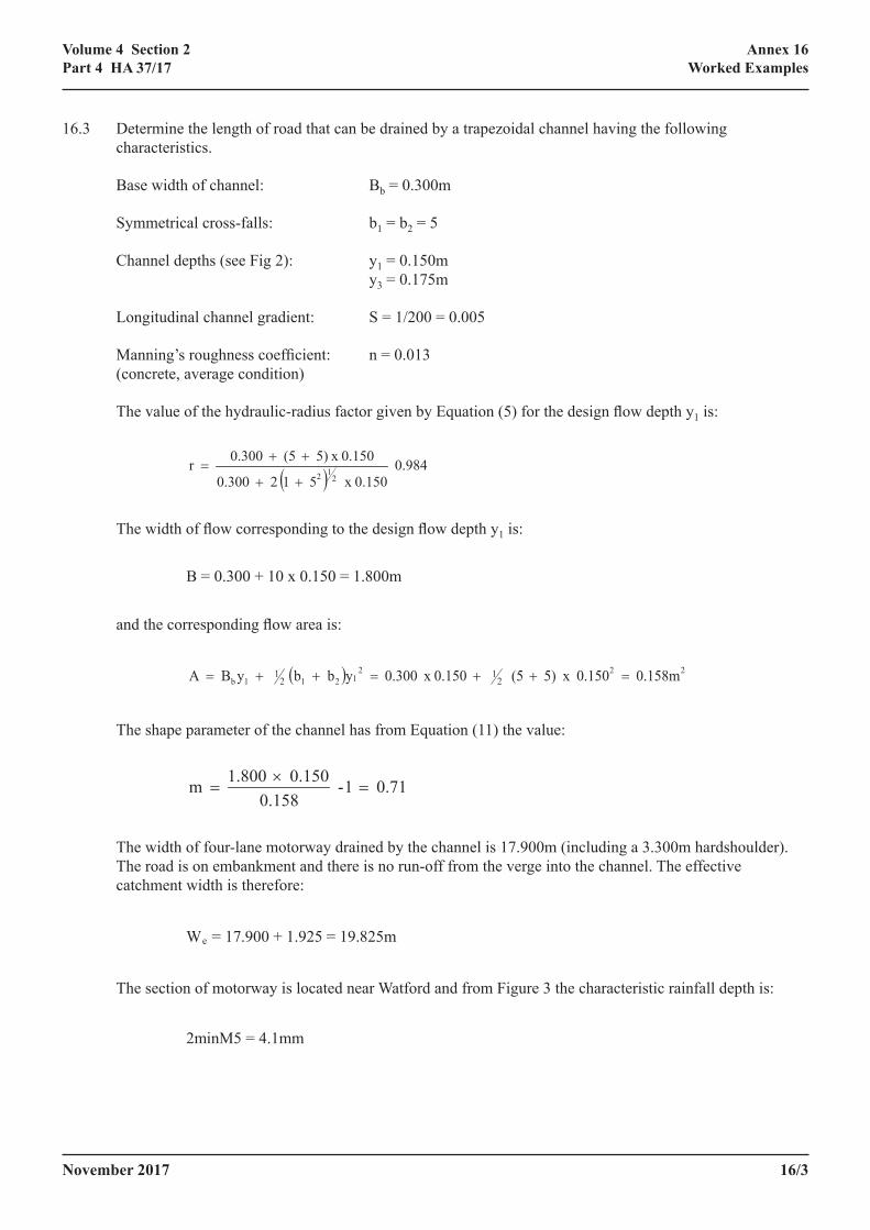
16.3 Determine the length of road that can be drained by a trapezoidal channel having the following characteristics.

Base width of channel: Bb = 0.300m

Symmetrical cross-falls: b1 = b2 = 5

Channel depths (see Fig 2): y1 = 0.150m y3 = 0.175m

Longitudinal channel gradient: S = 1/200 = 0.005

Manning’s roughness coefficient: n = 0.013 (concrete, average condition)

The value of the hydraulic-radius factor given by Equation (5) for the design flow depth y1 is:

Gm = 2.90 x 106 (2.65 - 1.00) = 4.79 x 106

2/31/2

6 0.120)x (0.981 013.0

(0.005) 10x 4.79 L =

244m 4.0x 10.625

0.0720 0.4) - (1.0 62.1

0.362- =

minutes 15.9 0.120)x (0.981 005.0

244x 0.013 0.085 T 2/3-2/1c =

=

We = 10.625 + 0.21 x 15.0 = 13.775m

160m 13.77510.625 244 L

62.1=

=

( )

0.984 0.150x 5 1 2 0.300

0.150x 5) (5 0.300 r 2

12++

++=

B = 0.300 + 10 x 0.150 = 1.800m

( ) 2221211b 0.158m 0.150x 5) (5 2

1 0.150x 0.300 yb b21 y B A =++=++=

0.71 1- 0.158

0.150 1.800 m =×

=

•

The width of flow corresponding to the design flow depth y1 is:

Gm = 2.90 x 106 (2.65 - 1.00) = 4.79 x 106

2/31/2

6 0.120)x (0.981 013.0

(0.005) 10x 4.79 L =

244m 4.0x 10.625

0.0720 0.4) - (1.0 62.1

0.362- =

minutes 15.9 0.120)x (0.981 005.0

244x 0.013 0.085 T 2/3-2/1c =

=

We = 10.625 + 0.21 x 15.0 = 13.775m

160m 13.77510.625 244 L

62.1=

=

( )

0.984 0.150x 5 1 2 0.300

0.150x 5) (5 0.300 r 2

12++

++=

B = 0.300 + 10 x 0.150 = 1.800m

( ) 2221211b 0.158m 0.150x 5) (5 2

1 0.150x 0.300 yb b21 y B A =++=++=

0.71 1- 0.158

0.150 1.800 m =×

=

•

and the corresponding flow area is:

Gm = 2.90 x 106 (2.65 - 1.00) = 4.79 x 106

2/31/2

6 0.120)x (0.981 013.0

(0.005) 10x 4.79 L =

244m 4.0x 10.625

0.0720 0.4) - (1.0 62.1

0.362- =

minutes 15.9 0.120)x (0.981 005.0

244x 0.013 0.085 T 2/3-2/1c =

=

We = 10.625 + 0.21 x 15.0 = 13.775m

160m 13.77510.625 244 L

62.1=

=

( )

0.984 0.150x 5 1 2 0.300

0.150x 5) (5 0.300 r 2

12++

++=

B = 0.300 + 10 x 0.150 = 1.800m

( ) 2221211b 0.158m 0.150x 5) (5 2

1 0.150x 0.300 yb b21 y B A =++=++=

0.71 1- 0.158

0.150 1.800 m =×

=

•

The shape parameter of the channel has from Equation (11) the value:

Gm = 2.90 x 106 (2.65 - 1.00) = 4.79 x 106

2/31/2

6 0.120)x (0.981 013.0

(0.005) 10x 4.79 L =

244m 4.0x 10.625

0.0720 0.4) - (1.0 62.1

0.362- =

minutes 15.9 0.120)x (0.981 005.0

244x 0.013 0.085 T 2/3-2/1c =

=

We = 10.625 + 0.21 x 15.0 = 13.775m

160m 13.77510.625 244 L

62.1=

=

( )

0.984 0.150x 5 1 2 0.300

0.150x 5) (5 0.300 r 2

12++

++=

B = 0.300 + 10 x 0.150 = 1.800m

( ) 2221211b 0.158m 0.150x 5) (5 2

1 0.150x 0.300 yb b21 y B A =++=++=

0.71 1- 0.158

0.150 1.800 m =×

=

•

The width of four-lane motorway drained by the channel is 17.900m (including a 3.300m hardshoulder). The road is on embankment and there is no run-off from the verge into the channel. The effective catchment width is therefore:

We = 17.900 + 1.925 = 19.825m

2minM5 = 4.1mm

Gm = 2.90 x 106 (2.65 - 0.71) = 5.63 x 106

322

16 0.150)x (0.984

013.0(0.005) 10x 5.63 L =

417m 4.1x 19.825

0.158 0.4) - (1.0 62.1

0.362- =

•

We = 17.900 + 1.000 = 18.900m

292.0437.0

21

4-

1.0000.150x 2 1

005.0

300x 0.013 10x 9.75 y

+

=

0.168m 4.1x 1.00018.900 0.4) - (5

708.00.158 =

•

The section of motorway is located near Watford and from Figure 3 the characteristic rainfall depth is: We = 17.900 + 1.925 = 19.825m

2minM5 = 4.1mm

Gm = 2.90 x 106 (2.65 - 0.71) = 5.63 x 106

322

16 0.150)x (0.984

013.0(0.005) 10x 5.63 L =

417m 4.1x 19.825

0.158 0.4) - (1.0 62.1

0.362- =

•

We = 17.900 + 1.000 = 18.900m

292.0437.0

21

4-

1.0000.150x 2 1

005.0

300x 0.013 10x 9.75 y

+

=

0.168m 4.1x 1.00018.900 0.4) - (5

708.00.158 =

•

16/4 November 2017



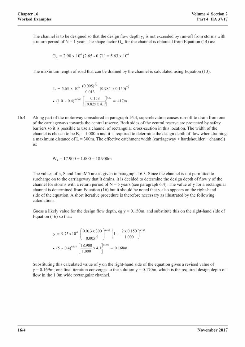
The channel is to be designed so that the design flow depth y1 is not exceeded by run-off from storms with a return period of N = 1 year. The shape factor Gm for the channel is obtained from Equation (14) as:

We = 17.900 + 1.925 = 19.825m

2minM5 = 4.1mm

Gm = 2.90 x 106 (2.65 - 0.71) = 5.63 x 106

322

16 0.150)x (0.984

013.0(0.005) 10x 5.63 L =

417m 4.1x 19.825

0.158 0.4) - (1.0 62.1

0.362- =

•

We = 17.900 + 1.000 = 18.900m

292.0437.0

21

4-

1.0000.150x 2 1

005.0

300x 0.013 10x 9.75 y

+

=

0.168m 4.1x 1.00018.900 0.4) - (5

708.00.158 =

•

The maximum length of road that can be drained by the channel is calculated using Equation (13):

We = 17.900 + 1.925 = 19.825m

2minM5 = 4.1mm

Gm = 2.90 x 106 (2.65 - 0.71) = 5.63 x 106

322

16 0.150)x (0.984

013.0(0.005) 10x 5.63 L =

417m 4.1x 19.825

0.158 0.4) - (1.0 62.1

0.362- =

•

We = 17.900 + 1.000 = 18.900m

292.0437.0

21

4-

1.0000.150x 2 1

005.0

300x 0.013 10x 9.75 y

+

=

0.168m 4.1x 1.00018.900 0.4) - (5

708.00.158 =

•

16.4 Along part of the motorway considered in paragraph 16.3, superelevation causes run-off to drain from one of the carriageways towards the central reserve. Both sides of the central reserve are protected by safety barriers so it is possible to use a channel of rectangular cross-section in this location. The width of the channel is chosen to be Bb = 1.000m and it is required to determine the design depth of flow when draining a maximum distance of L = 300m. The effective catchment width (carriageway + hardshoulder + channel) is:

We = 17.900 + 1.925 = 19.825m

2minM5 = 4.1mm

Gm = 2.90 x 106 (2.65 - 0.71) = 5.63 x 106

322

16 0.150)x (0.984

013.0(0.005) 10x 5.63 L =

417m 4.1x 19.825

0.158 0.4) - (1.0 62.1

0.362- =

•

We = 17.900 + 1.000 = 18.900m

292.0437.0

21

4-

1.0000.150x 2 1

005.0

300x 0.013 10x 9.75 y

+

=

0.168m 4.1x 1.00018.900 0.4) - (5

708.00.158 =

•

The values of n, S and 2minM5 are as given in paragraph 16.3. Since the channel is not permitted to surcharge on to the carriageway that it drains, it is decided to determine the design depth of flow y of the channel for storms with a return period of N = 5 years (see paragraph 6.4). The value of y for a rectangular channel is determined from Equation (16) but it should be noted that y also appears on the right-hand side of the equation. A short iterative procedure is therefore necessary as illustrated by the following calculations.

Guess a likely value for the design flow depth, eg y = 0.150m, and substitute this on the right-hand side of Equation (16) so that:

We = 17.900 + 1.925 = 19.825m

2minM5 = 4.1mm

Gm = 2.90 x 106 (2.65 - 0.71) = 5.63 x 106

322

16 0.150)x (0.984

013.0(0.005) 10x 5.63 L =

417m 4.1x 19.825

0.158 0.4) - (1.0 62.1

0.362- =

•

We = 17.900 + 1.000 = 18.900m

292.0437.0

21

4-

1.0000.150x 2 1

005.0

300x 0.013 10x 9.75 y

+

=

0.168m 4.1x 1.00018.900 0.4) - (5

708.00.158 =

•

Substituting this calculated value of y on the right-hand side of the equation gives a revised value of y = 0.169m; one final iteration converges to the solution y = 0.170m, which is the required design depth of flow in the 1.0m wide rectangular channel.

November 2017 17/1

Chapter 17Glossary of Symbols


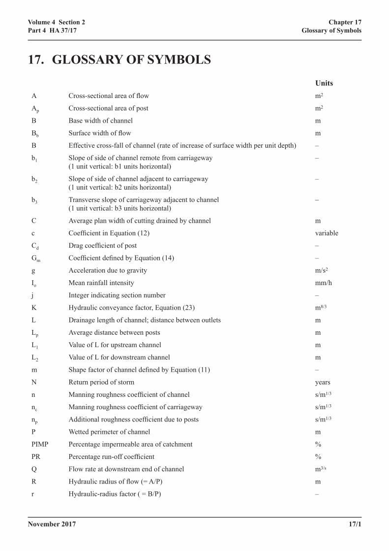
17. GLOSSARY OF SYMBOLS

UnitsA Cross-sectional area of flow m2

Ap Cross-sectional area of post m2

B Base width of channel m

Bb Surface width of flow m

B Effective cross-fall of channel (rate of increase of surface width per unit depth) –

b1 Slope of side of channel remote from carriageway (1 unit vertical: b1 units horizontal)

–

b2 Slope of side of channel adjacent to carriageway (1 unit vertical: b2 units horizontal)

–

b3 Transverse slope of carriageway adjacent to channel (1 unit vertical: b3 units horizontal)

–

C Average plan width of cutting drained by channel m

c Coefficient in Equation (12) variable

Cd Drag coefficient of post –

Gm Coefficient defined by Equation (14) –

g Acceleration due to gravity m/s2

Io Mean rainfall intensity mm/h

j Integer indicating section number –

K Hydraulic conveyance factor, Equation (23) m8/3

L Drainage length of channel; distance between outlets m

Lp Average distance between posts m

L1 Value of L for upstream channel m

L2 Value of L for downstream channel m

m Shape factor of channel defined by Equation (11) –

N Return period of storm years

n Manning roughness coefficient of channel s/m1/3

nc Manning roughness coefficient of carriageway s/m1/3

np Additional roughness coefficient due to posts s/m1/3

P Wetted perimeter of channel m

PIMP Percentage impermeable area of catchment %

PR Percentage run-off coefficient %

Q Flow rate at downstream end of channel m3/s

R Hydraulic radius of flow (= A/P) m

r Hydraulic-radius factor ( = B/P) –

17/2 November 2017

Chapter 17Glossary of Symbols


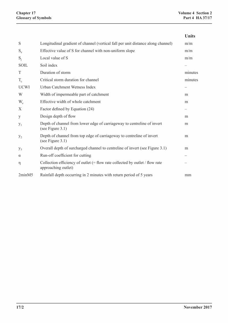
UnitsS Longitudinal gradient of channel (vertical fall per unit distance along channel) m/m

Se Effective value of S for channel with non-uniform slope m/m

Sj Local value of S m/m

SOIL Soil index –

T Duration of storm minutes

Tc Critical storm duration for channel minutes

UCWI Urban Catchment Wetness Index –

W Width of impermeable part of catchment m

We Effective width of whole catchment m

X Factor defined by Equation (24) –

y Design depth of flow m

y1 Depth of channel from lower edge of carriageway to centreline of invert (see Figure 3.1)

m

y2 Depth of channel from top edge of carriageway to centreline of invert (see Figure 3.1)

m

y3 Overall depth of surcharged channel to centreline of invert (see Figure 3.1) m

α Run-off coefficient for cutting –

η Collection efficiency of outlet (= flow rate collected by outlet / flow rate approaching outlet)

–

2minM5 Rainfall depth occurring in 2 minutes with return period of 5 years mm

November 2017 18/1

Chapter 18References


18. REFERENCESNormative

1. Manual of Contract Documents for Highway Works (MCHW) (HMSO)

Specification for Highway Works (MCHW 1)

Notes for Guidance on the Specification for Highway Works (MCHW 2)

Highway Construction Details (MCHW 3) – B Series

2. Design Manual for Roads and Bridges (DMRB) (HMSO)

HD 33 Design of Highway Drainage Systems (DMRB 4.2)

HD 45 Road Drainage and the Water Environment (DMRB 11.3.10)

HD 49: Highway Drainage Design Principal Requirements (DMRB 4.2.)

HD 50: The Certification of Drainage Design (DMRB 4.2)

TD 19 Requirements for Road Restraint Systems (DMRB 2.2)

HA 39 Edge of Pavement Details (DMRB 4.2) Section 6

HA 78 Design of Outfalls for Surface Water Channels (DMRB 4.2) Sections 6 and 7

HA 119 Grassed Surface Water Channels for Highway Runoff (DMRB 4.2)

3. BRITISH STANDARDS INSTITUTION. BS EN 12056: 2000, Gravity drainage systems inside buildings. Roof drainage layout and calculation.

Informative

4. FEH (1999). “Flood Estimation Handbook, Volume 2 Rainfall frequency estimation” by Faulkner D., Institute of Hydrology, UK, ISBN for volume 2: 0948540 90 7.

5. HR WALLINGFORD. The Wallingford Procedure: Design and Analysis of Urban Storm Drainage. 1981.

6. HR WALLINGFORD. Motorway Drainage Trial on the M6 Motorway, Warwickshire. TRRL Contractor Report 8, 1985.

7. IZZARD C F. Hydraulics of Runoff from Developed Surfaces. Highway Research Board (USA), Proceedings, 26, 1946, pp129 – 150.

8. FSSR16 (1985) Flood Studies Supplementary Report 16, Institute of Hydrology UK.

18/2 November 2017

Chapter 18References


November 2017 19/1

Chapter 19Approval


19. APPROVALApproval of this document for publication is given by:

Department for InfrastructureClarence Court10-18 Adelaide StreetBelfast P B DOHERTY BT2 8GB Director of Engineering

Welsh GovernmentTransport S HAGUECardiff Deputy DirectorCF10 3NQ Network Management Division

Transport Scotland8th Floor, Buchanan House58 Port Dundas RoadGlasgow R BRANNENG4 0HF Chief Executive

Highways EnglandTemple Quay HouseThe SquareTemple QuayBristol M WILSONBS1 6HA Chief Highway Engineer

All technical enquiries or comments on this Document should be sent to [email protected]

19/2 November 2017

Chapter 19Approval


November 2017 A/1


Annex ARainfall Data

ANNEX A RAINFALL DATAA.1 The Meteorological office is able to provide individual data on rainfall characteristics for any location in

the UK. However, in order to produce a general design method for surface water channels, it is necessary to be able to describe the rainfall characteristics by means of an equation relating mean intensity to the duration and return period of the storm event. The rainfall intensity used in the equation should be increased to allow for climate change by the percentage stated in HD33 [Ref 2].

A.2 Relevant information on short-period storms with durations between 1 minute and 10 minutes was provided by the Met Office for use in BSEN 12056:2000 [Ref 3]. The following general calculation procedure is given in Annex A of BSEN 12056

(a) Determine from a map of the UK (reproduced in this document as Figure 7.1) the value of rainfall depth (2minM5) occurring in 2 minutes with a return period of 5 years at the chosen location.

(b) Calculate (using a table and the value of 2minM5) the rainfall depth for the required duration T but still with a return period of 5 years (ie TminM5)

(c) Calculate (using a graph and the value of TminM5) the rainfall depth for the required duration T and return period N (ie TminMN).

(d) Divide the rainfall depth TminMN by the duration to give the mean intensity I0.

A.3 Equation (10) for predicting I0 was obtained for this document by curve-fitting the tabular and graphical data corresponding to steps (b) to (d) above. The applicability of the equation to storm durations greater than 10 minutes was checked using data in Volume II of the Flood Estimation Handbook [Ref 4]. The equation is optimized for values of T = 2-20 minutes and N = 1-20 years and tends to overestimate I0 (ie err on the safe side) outside these ranges. The recommended upper limits for use of Equation (10) are T = 30 minutes and N = 50 years.

A.4 The critical storm duration Tc that gives rise to the design flow conditions in a particular channel can be estimated from:

32-

21c (ry)

S

nL 0.085 T

=

(A.1)

where Tc is in minutes and the units for the other quantities are as defined in paragraph 5.3.

A/2 November 2017


Annex ARainfall Data

November 2017 B/1


Annex BChannel Roughness

ANNEX B CHANNEL ROUGHNESSB.1 The Manning resistance equation is appropriate when a flow is rough-turbulent (ie, with its resistance

mainly determined by the surface texture of the channel). This is likely to be the case in most road drainage channels, except perhaps near the upstream end where the velocity or depth of flow is small and the flow may be smooth- turbulent (ie, with its resistance mainly determined by the viscosity of the water). It is often assumed that the roughness coefficient n depends only upon the surface texture of the channel, but experimental evidence indicates that it can vary with the relative depth of flow, the cross-sectional shape of the channel and the intensity of any lateral inflow.

B.2 A modified version of Manning’s equation for shallow triangular channels was developed by Izzard [Ref 7] and is recommended by the US Federal Highway Administration. The equation has the form:

382

1

yn

bS 83 Q =

(B.1)

and is obtained by applying Manning’s equation to vertical elements in the cross-section and integrating the discharge across the channel; no allowance is made for the resistance of a vertical kerb. Equation (B.1) gives capacities that are approximately 20% higher than the conventional version in Equation (6). Values of n quoted in the literature for triangular channels therefore depend upon which of the two formulae were used to analyse the experimental data.

B.3 The conventional form of Manning’s equation has been used in this document (ie, Equations (1), (3), (6) and (8)) so as to provide a common basis for all shapes of channel. Values of n given in the literature vary typically from 0.010 to 0.017 for concrete channels and from 0.012 to 0.022 for asphalt channels. In Table 11.1 the recommended figures for “average” condition correspond approximately to the mean of the published values; the figures for “poor” condition are slightly less than the corresponding maximum values.

B.4 Factors which will tend to increase the resistance of a channel are lateral inflow from the road surface and the presence of silt and grit in the invert. Data on these effects are not available, but it is probable that at the downstream ends of channels (which are the most critical points) they are not very large in relation to the uncertainties in the basic n values. An “average” value of n = 0.013 for a concrete channel would be appropriate if it has a trowel-type finish, no sharp discontinuities in line or elevation, and is regularly cleaned.

B.5 An approximate procedure is given in Chapter 13 for applying the design method for simple cross-sectional shapes to the case of surcharged compound channels. It was found that a direct solution for compound channels could be obtained only when using a development of the modified Manning’s equation in Equation (B.1). The relationships in Equations (21) to (25), between the relevant hydraulic characteristics (flow capacity and storage capacity) for a compound channel and an equivalent “simple” channel, are therefore based on the modified form of Manning’s equation.

B.6 Equation (19) in paragraph 11.2 for estimating the extra flow resistance produced by a longitudinal line of posts is obtained by considering the drag force acting on each post. The factor of 0.7 in the equation corresponds to a drag coefficient of Cd = 1.2 with an allowance for the effect of varying water depth between the upstream and downstream ends of a channel.

B/2 November 2017


Annex BChannel Roughness

November 2017 C/1


Annex CRun-Off from Cuttings

ANNEX C RUN-OFF FROM CUTTINGSC.1 In the absence of suitable published data, it was decided to use an existing run-off equation to provide a

method for estimating run-off from road cuttings. The selected equation was developed during studies for the Wallingford Procedure [Volume 1 of Ref 5] as a means of predicting surface run-off to urban storm sewers in the UK, and has the form:

PR = 0.662 PIMP + 0.00219 (100 - PIMP). SOIL. UCWI

C 300

SOIL.UCWI W We

+=

(C.1)

where PR is the percentage run-off from the whole catchment, PIMP is the percentage of impervious area, SOIL is a number related to the infiltration potential of the soil and UCWI is an index of the urban catchment wetness. [A different run-off formula was finally adopted for the Wallingford Procedure, but Equation (C.1) is more suitable for application to roads in cuttings].

C.2 The effective width We of a road in cutting is defined as the equivalent width of road which will produce the same total amount of run-off as a road of width W and a cutting of average width C. From Equation (C.1) it can be shown that:

PR = 0.662 PIMP + 0.00219 (100 - PIMP). SOIL. UCWI

C 300

SOIL.UCWI W We

+=

(C.2)

C.3 The Flood Studies Supplementary Report 16 (FSSR16)] [Ref 8] classified UK soils into five Soil Classes, S1 to S5 according to their infiltration potential. These SOIL parameters are between 0.10 and 0.53; the lowest value would apply to a well-drained sandy soil and the highest to a rocky soil on a fairly steep slope. Maps showing regional distributions of SOIL classes are given in Volume 5 of Ref 4 and Volume 3 of Ref 5; the type of soil in a cutting should, however, be assessed from a site survey since the maps do not identify small local variations. Cuttings for roads are steeper than most natural catchments, and for a given soil type may produce relatively more run-off. Approximate allowance can be made for this by classifying a soil in a category of lower infiltration potential than normal; values of the SOIL parameter for cuttings might therefore be expected to be in the range 0.3 to 0.53.

C.4 Design values of UCWI for use with Equation (C.1) are given in Volume 1 of Ref 5 as a function of the standard average annual rainfall at a site. Representative values for UK regions were obtained by finding the maximum range of UCWI within each region (excluding only peaks in highland areas), and adopting a figure one third of this range below the maximum value. The regions were then grouped into categories of high, medium and low catchment wetness, and an average representative value of UCWI calculated for each group.

C.5 The values of the run-off coefficient α in Table 12.1 were obtained from Equation (C.2) using figures of SOIL = 0.3, 0.47 and 0.53 for soils of high, medium and low permeability, and representative values of UCWI = 71, 107, and 132 for low, medium, and high categories of antecedent wetness.

C.6 Site data should be collected where possible to improve the estimate of run-off from the cuttings.

C/2 November 2017


Annex CRun-Off from Cuttings

November 2017 D/1


Annex DList of Amendments from Previous Version

ANNEX D LIST OF AMENDMENTS FROM PREVIOUS VERSION

Amend No

Page No

Signature & Date of incorporation of amendments

Amend No

Page No

Signature & Date of incorporation of amendments

01/17 Full Clause changes have been made throughout the document to make it compliant with the CPR. References which have been superseded by hENs or ETAs have been replaced with the relevant hEN/ETA. The Normative and Informative References have been updated accordingly.

Various other minor, non-material changes have been made to the text.

Requirement for climate change to be taken into account added to Section 7.1

D/2 November 2017


Annex DList of Amendments from Previous Version