Embed Size (px)
Citation preview

i
Volume: 4
Issue : 1
Year : 2016

ii
Volume 4 / Issue 1
Journal of Engineering and Science
Editor in Chief (Owned By Academic Platform)
Prof.Dr.Mehmet SARIBIYIK, Sakarya University, Turkey
Editors
Prof.Dr. Barış Tamer TONGUÇ, Sakarya University, Turkey
Assoc. Prof. Dr. Fatih ÇALIŞKAN, Sakarya University, Turkey
Asst. Prof. Dr. Hakan ASLAN, Sakarya University, Turkey
Support
Lec. Gökhan ATALI, Sakarya University, Turkey
Members of Advisory Board
Prof. Dr. Abdullah Çavuşoğlu, Council of Higher Education, Turkey
Prof. Dr. Mehmet Emin AYDIN, University of West of England, England
Prof. Dr. Erol ARCAKLIOĞLU, The Scientific and Technological Research Council of Turkey
Prof. Dr. Fahrettin ÖZTÜRK, The Petroleum Institute, The United Arab Emirates
Prof. Dr. Ahmet TÜRK, Celal Bayar University, Turkey
Contact
Academic Platform
http://apjes.com/

iii
Journal of Engineering and Science
Contents Image Damage Analysis With Morphological Image Processing Technique Using Artificial Neural Networks
1-7
Engineering Models of Masonry by Joint Repairing Techniques
8-14
Development and Characterization of Parian Bodies Using Feldspar from Two Selected Deposits in Nigeria
15-20
Fractional Distribution of Heavy Metals from the Tailings of Itagunmodi Goldmine Site Osun State, Nigeria
21-27
The Solution of Shift Scheduling Problem by Using Goal Programming
28-37
Design of a Novel Architecture for QPSK Modulator
38-47

iv
Journal of Engineering and Science
İçindekiler Morfolojik Görüntü İşleme Tekniği ile Yapay Sinir Ağlarında Görüntü Tahribat Analizi
1-7
Engineering Models of Masonry by Joint Repairing Techniques
8-14
Development and Characterization of Parian Bodies Using Feldspar from Two Selected Deposits in Nigeria
15-20
Fractional Distribution of Heavy Metals from the Tailings of Itagunmodi Goldmine Site Osun State, Nigeria
21-27
Hedef Programlama ile Nöbet Çizelgeleme Probleminin Çözümü
28-37
Yeni Bir QPSK Modülatör Mimarisinin Tasarımı
38-47

G. ATALI/APJES IV-I (2016) 01-07
*Corresponding author: Address: Sakarya Meslek Yüksekokulu, Mekatronik Programı Sakarya Üniversitesi, 54187,
Sakarya TÜRKİYE. E-mail address: [email protected], Telefon: +902642953495
Doi:10.21541/apjes.27271
Morfolojik Görüntü İşleme Tekniği ile Yapay Sinir Ağlarında
Görüntü Tahribat Analizi
*1Gökhan Atalı, 2S.Serdar Özkan, 2Durmuş Karayel
*1Sakarya Meslek Yüksekokulu, Mekatronik Programı Sakarya Üniversitesi, Türkiye 2Teknoloji Fakültesi, Mekatronik Mühendisliği Sakarya Üniversitesi, Türkiye
Geliş Tarihi: 2015-12-25 Kabul Tarihi: 2016-04-09
Öz
Teknolojinin gelişmesine paralel olarak kamera sistemlerinde yüksek düzeyde kaliteyi öngören lensler tasarlanmıştır.
Ancak bu lensler yapısal olarak her ne kadar görüntü kalitesinde başarılı olsalar da üzerinde tahribat meydana gelmiş
görüntülerin ayırt edilmesinde herhangi bir ek özellik mevcut değildir. Esasen bu tür tahribatların giderilmesi için
yapay zeka teknikleri kullanmak mümkündür. Bu çalışmada, yapay sinir ağları kullanarak üzerinde tahribat meydana
gelmiş görüntülerin morfolojik görüntü işleme teknikleri ile birleştirilerek tahribatın derecesine göre orijinal görüntüye
yakınsaması ele alınmıştır. Ayrıca bu amaca ulaşmak ve kullanımı kolaylaştırmak amacıyla geliştirilen arayüz
sayesinde eğitim ve test verilerinin yanı sıra ağı oluşturmak için kullanılacak parametrelerin kolaylıkla hazırlanan
algoritmaya entegrasyonu sağlanmaktadır.
Anahtar Kelimeler: Yapay Sinir Ağları, Karakter Tespiti, Morfolojik Görüntü İşleme
Image Damage Analysis With Morphological Image Processing Technique
Using Artificial Neural Networks
*1Gökhan Atalı, 2S.Serdar Özkan, 2Durmuş Karayel
1Sakarya Meslek Yüksekokulu, Mekatronik Programı Sakarya Üniversitesi, Türkiye 2Teknoloji Fakültesi, Mekatronik Mühendisliği Sakarya Üniversitesi, Türkiye
Abstract
The lenses providing high quality for camera systems are designed as parallel with developing technologies. These
lenses do not have any additional functionality to distinguish damaged images while they are successful with regard
to image quality. Essentially, artificial intelligence techniques can be used to eliminate such damaged cases. In this
study, convergence to original image of the damaged images according to the degree of damage using together artificial
neural networks and morphological image processing techniques are discussed. Also, it is provided to be integrated
training and test data with used algorithm thanks to developed interfaces to achieve goal and to facilitate use. In
addition, this interface is used to be entered the training parameters to the system.
Keywords: Artificial Neural Networks (ANN), Character detection, Morphological image processing
1. Giriş
Günümüzde birçok alanda morfolojik görüntü işleme
teknikleri ile çeşitli analizler yapılmaktadır. Bunlardan
en bilinenleri; araç plakası tanıma, bant üzerindeki
ürünlerin tanımlanması, cisimlerin çap ve boy
uzunlukları için görüntü analizleridir. Görüntü işleme
esasen görüntünün sayısallaştırılarak veri setlerine
dönüştürülmesi ve çeşitli yöntemlerle işlenmesi olarak
tanımlanır. Bu konu ile ilgili yapılan çalışmalar
incelendiğinde araştırmacıların; kenar ayrıştırma,
Hough dönüşümü, simetri özelliği, renk özelliği,
histogram analizi, Gabor süzgeçleri gibi görüntü
işleme tekniklerini kullandıkları görülmektedir [1-8].

G. ATALI/APJES IV-I (2016) 01-07
Bu konu hakkında Literatür incelendiğinde; Fatih
Kahraman ve arkadaşları aktif görünüm modeline
dayalı yüz tanıma isimli çalışmalarında insan yüzünün
temel bileşenlerini otomatik olarak saptayan aktif
görünüm modeline ve Gabor süzgeçlerine dayalı bir
yüz tanıma yöntemi geliştirmişlerdir [9]. C.Tu ve
arkadaşları Hough dönüşümünü kullanarak araçların
belirli bir rota üzerindeki pozisyonlarının bulunmasını
amaçlamış ve bu konuda bir çalışma
gerçekleştirmişlerdir [10]. C. Lopez-Molina ve
arkadaşları ayrıt saptama yöntemine ait performans
analizleri üzerine çalışma yapmışlardır [11].
Görüntü üzerinde yer saptama için en yaygın olarak
kullanılan yöntemlerin başında ayrıt saptama ve
eşikleme tabanlı yöntemler gelmektedir. Ayrıt saptama
ve eşikleme giriş görüntüsünü 1 ve 0 bilgilerinden
oluşan ikili resme dönüştürmek için kullanılır. Daha
sonra elde edilen bu ikili resmin dikey ve yatay
izdüşüm histogramları analiz edilerek resmin üzerinde
istenilen bölgeler tespit edilir [12-17]. Diğer bir
yöntemde ayrıtlar bulunduktan sonra Hough
dönüşümü uygulanarak resmin çevresi bulunmaktadır
[18]. Bahsedilen bu yöntemler ile elde edilen ikili
moda dönüştürülmüş sayısal görüntü üzerinde
morfolojik açma ve kapama gibi işlemler uygulanarak
görüntüyü gerçek halinden uzaklaştırmak mümkündür.
Esasen burada gerçek görüntüden uzaklaşmadan
maksat, görüntü üzerinde tahribat meydana geldiği
manasındadır. Çevre şartlarından ve metnin yazılı
olduğu zeminden kaynaklı problemler gibi birçok
olumsuz etki görüntü üzerine yansımakta ve görüntüyü
gerçek halinden uzaklaştırmaktadır.
Bu çalışmada bahsedilen bu etkilere benzer şekilde
görüntü üzerinde morfolojik açma ve kapama işlemleri
uygulanarak görüntü üzerinde tahribat meydana
getirilmiştir. Üzerinde değişiklik meydana gelerek
farklı bir görüntü haline gelen yeni görüntü, tahribat
analizi yaparak doğruya yaklaşımda bulunan bir yapay
sinir ağına (YSA) test verisi olarak sunulmuş ve analiz
edilmiştir. Bu işlemler sırasında eğitim verileri için
hazırlanan resimler üzerinde ayrıt saptama, eşikleme
yöntemleri kullanılmış ardından oluşan ikili bilginin
dikey yatay izdüşümleri bir veri setine dönüştürülerek
MATLAB ortamında yapay sinir ağları tarafından
oluşturulan bir ağa eğitim verisi olarak tanıtılmıştır.
Ayrıca çalışmada MATLAB ortamında bir arayüz
tasarlanarak veri setlerinin eğitimi ve testleri için
uygulanacak fonksiyon çeşitleri, ara katman sayısı, ara
katmandaki nöron sayısı, açma-kapama miktarı gibi
bilgilerin dışarıdan müdahale ile değiştirilebilir olması
sağlanmıştır.
2. Yapay Sinir Ağları ve Görüntü İşleme
Yapay Sinir Ağları (YSA), insan beyninin bilgi işleme
tekniğinden esinlenerek geliştirilmiş bir bilgi işlem
teknolojisidir. YSA ile basit biyolojik sinir sisteminin
çalışma şekli simüle edilmektedir. Simüle edilen sinir
hücreleri nöronlar içerirler ve bu nöronlar çeşitli
şekillerde birbirlerine bağlanarak ağı oluştururlar. Bu
ağlar öğrenme, hafızaya alma ve veriler arasındaki
ilişkiyi ortaya çıkarma kapasitesine sahiptirler. Diğer
bir ifadeyle, YSA'lar, normalde bir insanın düşünme ve
gözlemlemeye yönelik doğal yeteneklerini gerektiren
problemlere çözüm üretmektedir. Bir insanın,
düşünme ve gözlemleme yeteneklerini gerektiren
problemlere yönelik çözümler üretebilmesinin temel
sebebi ise insan beyninin ve dolayısıyla insanın sahip
olduğu yaşayarak veya deneyerek öğrenme
yeteneğidir. Görüntü işleme ölçülmüş veya
kaydedilmiş olan dijital görüntü verilerini, elektronik
ortamda çeşitli yazılımlar ile amaca uygun şekilde
değiştirmeye yönelik yapılan çalışmaları
kapsamaktadır. Görüntü işleme, daha çok, kaydedilmiş
olan, mevcut görüntüleri işlemek, yani mevcut resim
ve grafikleri, değiştirmek, yabancılaştırmak ya da
iyileştirmek için kullanılmaktadır.
3. Morfolojik Görüntü İşleme
Matematiksel morfoloji, lineer olmayan komşuluk
işlemlerinde güçlü bir görüntü işleme analizidir.
Morfolojik görüntü işlemede genişletme ve aşındırma
isimli temel iki işlem kullanılmaktadır. Morfolojik
görüntü işlemede bilinen açma ve kapama işlemleri
gibi diğer tüm yöntemler bu iki işlemi referans alarak
gerçekleştirilir. Üzerinde kare ve daire gibi geometrik
şekillerle yapısal filtre uygulanan görüntü açma veya
kapama gibi morfolojik işlemlere tabi tutulur. Ancak
görüntü üzerinde yapısal filtre uygulayarak genişletme
veya aşındırma işlemi yapabilmek için görüntü önce
binary (ikili) moda çevrilir.
3.1. Genişletme İşlemi
İkili moda dönüştürülen görüntü üzerinde büyütme ya
da kalınlaştırma işlemlerinin yapıldığı morfolojik
işlemleri kapsamaktadır. Sayısal bir resmi genişletmek
resmi yapısal elemanla kesiştiği bölümler kadar
büyütmek demektir. Kalınlaştırma işleminin nasıl
yapılacağını Şekil 3’te örnek verilen yapı elemanları
belirler. Şekil 1 de görüldüğü üzere üzerinde
genişletme yapılan sayısal görüntüde açma meydana
gelmiş ve dolayısıyla görüntüde normalin dışına çıkan
bir bozulma gözlenmektedir.

G. ATALI/APJES IV-I (2016) 01-07
Şekil 1. 3x3 yapısal elemanı ile genişletme işlemi
3.2. Aşındırma İşlemi
İkili moda dönüştürülen görüntü üzerinde küçültme ya
da inceltme işlemlerinin yapıldığı morfolojik işlemleri
kapsamaktadır. Aşındırma işlemi bir bakıma
genişletme işleminin tersidir. Aşındırma işlemi ile
sayısal resim üzerinde inceltme yapılmış dolayısıyla
görüntüde tahribat meydana gelmiş olur.
Aşındırmadan kaynaklı bu tahribat sonucunda resim
içerisindeki nesneler boyutsal olarak daralır, delik
varsa genişler ve bağlı nesneler ayrılma eğilimi
gösterir. Şekil 2 de aşındırma işlemi için bir örnek
görüntü verilmiştir.
Eğer sayısal bir görüntüye genişletme ve aşındırma
işleminin ardışık olarak uygulanırsa görüntüde açma
işlemi meydana gelmektedir. Açma işleminde birbirine
yakın iki nesne görüntüde fazla değişime sebebiyet
vermeden ayrılmış olurlar. Açmanın tersi olarak
sayısal görüntü üzerinde aşındırma ve genişletme
işleminin ardışık uygulanmasıyla da kapama işlemi
meydana gelmektedir. Dolayısıyla birbirine yakın iki
nesne görüntüde fazla değişiklik yapılmadan birbirine
bağlanmış olur. Bu işlemlerin matematiksel gösterimi
şu şekildedir;
Genişletme: A B
Aşındırma: A B
Açma işlemi: A o B =( A B ) B
Kapama işlemi: A ● B =( A B ) B
Yapısal eleman olarak adlandırılan ifade istenilen
boyutlarda ve istenilen şekilde hazırlanmış matris
formunda yapıları içermektedir. Yapısal eleman çeşitli
geometrik şekillerden biri olabilmektedir; en sık
kullanılan yapısal elemanlar kare, dikdörtgen ve daire
şeklindedir. Yapısal eleman örnekleri Şekil 3’ te
gösterilmiştir. Eğer morfolojik işlem olarak resimdeki
nesnelerin keskin hatları silinip yerlerine kavisli veya
daha yumuşak hatlar getirilmek isteniyorsa dairesel
yapısal eleman kullanılmalıdır.
4. Uygulama Çalışması
Bu çalışmada yapay sinir ağları ile üzerinde morfolojik
görüntü işleme teknikleri uygulanmış sayısal
görüntünün daha önceden ağa tanıtılan orijinal
resimler ile karşılaştırılması ve ağın doğruya
yaklaşımları incelenmiştir. Bu yaklaşımları
yapabilmek için Şekil 4'te verilen yol ve yöntemler
sırası ile gerçekleştirilmiştir.
4.1. Eğitim verilerinin alınması
Geliştirilen bir ara yüz aracılığı ile ağda eğitime tabii
tutulacak görüntülerin alınması bu basamakta
gerçekleştirilmektedir. Ağda eğitilmesi düşünülen veri
setleri 27x27 pixel boyutlarında (yaklaşık 18-24 punto)
resimlerden oluşmaktadır. Bu resimler 50x50
boyutlarında sayısal 1 ve 0 değerlerinden oluşan
sayısal veri seti haline getirildikten sonra 2500x1 sütun
matrisine dönüştürülmektedir. Bu sayede görüntü
yapay sinir ağlarında kullanılmak üzere hazır bir
eğitim veri setine dönüştürülür. Veri seti olarak
aşağıdaki gibi kullanılmıştır. Bu veri setlerinin %20'si
eğitim için, diğer %80'i ise test için kullanılmıştır.
Şekil 2. 3x3 yapısal elemanı ile aşındırma işlemi
0 1 0
1 1 1
0 1 0
0 1 1
1 0 1
1 1 0
1 0 1
0 1 0
1 0 1
Şekil 3. Yapısal eleman örnekleri

G. ATALI/APJES IV-I (2016) 01-07
Şekil 4. Uygulamanın gerçekleşme basamakları
4.2. Oluşturulacak ağ için parametrelerin
belirlenmesi ve ağın eğitimi
Yapay sinir ağı oluşturmak için gerekli eğitim,
performans ve transfer fonksiyonları ile ağda
ulaşılması hedeflene nihai değer için gerekli
parametrelerin girişi bu basamakta sağlanır. Ayrıca ilk
katmandaki nöron sayısı ve maksimum epoch (devir)
değeri de yine bu basamakta girilen parametreler
arasında yer alır. Bu parametreler yapay sinir ağları
oluşturulurken esas alınan temel parametrelerdir. Bu
çalışmada izlenen yöntem ve teknikler için en uygun
parametre dizisi Tablo 1 de verilmiştir.
Tablo 1 de belirtilen parametreler dahilinde ağa
sunulan eğitim verilerinin eğitimi sonucu Şekil 5 ve
Şekil 6 da görüldüğü üzere regresyon değeri 0.999,
gradyan değeri ise 148 iterasyonda 0.00010054 olarak
saptanmıştır.
4.3. Test verilerinin alınması ve morfolojik teknik
uygulanması
Eğitilmiş ağda test etmek üzere test verilerinin
alınması ve morfolojik teknik uygulayarak görüntü
üzerinde tahribat meydana getirilmesi bu basamakta
gerçekleştirilmiştir. Test verilerinin ağda eğitilmek
üzere dosyadan alınması eğitim verileri için izlenen
yöntem ve teknik ile aynıdır. Görüntüler
sayısallaştırıldıktan sonra sayısal veri setine 1, 2, 3 ve
4 derecelik dairesel ortalama filtresi ayrı ayrı
uygulanmış ve görüntü orijinalliğinden
uzaklaştırılarak, görüntüde tahribat meydana
getirilmiştir (Şekil 7). Üzerinde değişiklik yapılan
görüntü köşe bulma yöntemi ve ayrıt saptama tekniği
ile uygun matris formuna dönüştürülmüş ve yapay
sinir ağına test verisi olarak sunulmuştur. Daha sonra
orijinal görüntü ile üzerinde tahribat meydana gelmiş
görüntü metinsel ve görüntü olarak incelemeye tabii
tutulmuş ve çıkarımda bulunulmuştur.
Şekil 5. Ağın eğitimi
Eğitim verilerinin alınması
Oluşturulacak ağ için parametrelerin
belirlenmesiAğın eğitilmesi
Test verilerinin alınması
Test verilerine morfolojik teknik
uygulanması
Test verilerini oluşturulan ağda
eğitimi
Sonuçlar ve karşılaştırma

G. ATALI/APJES IV-I (2016) 01-07
Şekil 6. Ağın eğitim sonuçları
Tablo 1. Belirlenen ağ parametreleri
Eğitim fonk.
Performans
fonksiyonu
Transfer fonk. Max.
Epoch
Hedef İlk katmandaki nöron
sayısı
trainscg mse Logsig 1000 1e-5 10
Şekil 7. 4 derecelik dairesel ortalama filtresi uygulanmış görüntü
5. Sonuçlar ve Tartışma
Görüntüler üzerinde çeşitli etkenlerden dolayı
meydana gelen tahribatlar, morfolojik görüntü işleme
platformundan yararlanılarak görüntü üzerinde
oluşturulmuş ve yapay sinir ağları kullanılarak
üzerinde tahribat meydana gelmiş görüntünün gerçeğe
yakınlığı test edilmiştir. Görüntüde meydana
gelebilecek bu tahribatlar dört farklı derecede dairesel
ortalama filtresinin görüntüye uygulanması ile
gerçekleşmiş ve sonuç olarak elde edilen değerler
Tablo 2 ve Şekil 8’de sunulmuştur. Bu değerlere göre
geliştirilen yapay sinir ağında, 2 ve 3 derecelik dairesel
ortalama filtresi ile oluşturulan morfolojik görüntüde
ortalama yüzde 75 başarım sağlanırken aşınma şayet 4
dereceye çıkarılırsa görüntünün orijinalliğinden
oldukça uzaklaşması sebebiyle yaklaşımda da
azalmanın görüldüğü sonucuna varılmıştır. Ayrıca
tablo 2 de bahsi geçen yaklaşımlar var-yok olarak
nitelendirilmiş ve bu doğrultuda yüzde olarak ifade
edilmiştir. İlerleyen çalışmalarda yaklaşım değerleri
fuzzy lojik ya da neuro fuzzy kullanılarak geniş
aralıklarda ifade edilebilir. Meydana gelebilecek
tahribatın Gaussian alçak geçiren filtresi, motion

G. ATALI/APJES IV-I (2016) 01-07
hareket benzetimi filtresi gibi değişik filtreler altında
da incelenmesi sağlanabilir. Ayrıca bu çalışmadakine
benzer uygulamaları içeren kamera lensleri
tasarlanarak görüntülerin algı esnasında analizleri
sağlanabilir.
Tablo 2. YSA yaklaşım karşılaştırmaları
Test verisi
Morfolojik
sonuç
Açma
Derecesi Yaklaşım (%) Yaklaşım (%)
Açma
Derecesi
Morfolojik
sonuç
Test
verisi
A A 3 100 100 4 A A
B C 3 0 0 4 A B
C C 3 100 100 4 C C
D D 3 100 0 4 C D
AC AC 3 100 100 4 AC AC
AD AC 3 50 50 4 AC AD
ACB ACA 3 66 66 4 ACC ACB
BAC BAC 3 100 66 4 AAC BAC
CAB CAB 3 100 66 4 CAD CAB
CBA CBA 3 100 66 4 CDA CBA
ABCD ACCD 3 50 50 4 ADCA ABCD
Ortalama Yaklaşım : 78,727 60,364
Şekil 8. 1-2-3-4 derecelik açma derecelerine karşı YSA yaklaşımı
69,45573,364 78,727
60,364
0
20
40
60
80
100
1 2 3 4
Yak
laşı
m (
%)
Açma derecesi
YSA yaklaşımı
Test verisi
Morfolojik
sonuç
Açma
Derecesi Yaklaşım (%) Yaklaşım (%)
Açma
Derecesi
Morfolojik
sonuç
Test
verisi
A A 1 100 100 2 A A
B C 1 0 0 2 A B
C C 1 100 0 2 D C
D D 1 100 100 2 D D
AC AC 1 100 100 2 AC AC
AD AC 1 50 100 2 AD AD
ACB ACD 1 66 100 2 ACB ACB
BAC CAC 1 66 100 2 BAC BAC
CAB CAD 1 66 66 2 CAC CAB
CBA CDA 1 66 66 2 CCA CBA
ABCD ACCD 1 50 75 2 ABCA ABCD
Ortalama Yaklaşım: 69,455 73,364

G. ATALI/APJES IV-I (2016) 01-07
Referanslar
[1] Barroso, J., Rafael, A., Dagless, E. L., Bulas-Cruz,
J., Number plate reading using computer vision, IEEE
– International Symposium on Industrial Electronics
ISIE’97, Universidade do Minho, Guimarães, 1997.
[2] Morphological Segmentation for Textures and
Particles, Published as Chapter 2 of Digital Image
Processing Methods, E. Dougherty, Editor, Marcel-
Dekker, New York, 1994, Pages 43--102.
[3] B. Hongliang and L. Changping. A hybrid license
plate extraction method based on edge statistics and
morphology.17th International Conference On Pattern
Recognition(ICPR’04), 2:831–834, 2004.
[4] M. Sarfraz, M. J. Ahmed, and S. A. Ghazi. Saudi
arabian license plate recognition system. Proceedings
of the 2003 International Conference on Geometric
Modeling and Graphics(GMAG’03), pages 36–41,
2003.
[5] V. Kamat and S. Ganesan. An efficient
implementation of hough transform for detecting
vehicle license plate using dsp’s. 1st IEEE Real-Time
Technology and Applications Symposium, pages 58–
59, 1995.
[6] V. Shapiro, D. Dimov, S. Bonchev, V. Velichkov,
and G. Gluhchev. Adaptive license plate image
extraction. International Conference on Computer
Systems and Technologies, 2003.
[7] F. Mart´ın, M. Garc´ıa, and J. L. Alba. New
methods for automatic reading of vlps (vehicle license
plates). Signal Processing Patten Recognition and
Application, 2002.
[8] Kahraman F., Gökmen M. “GABOR Süzgeçler
Kullanılarak Taşıt Plakalarının Yerinin Saptanması”,
11. sinyal İşleme ve İletişim Uygulamaları Kurultayı,
İstanbul, 2003.
[9] F. Kahraman, B.Kurt, M.Gökmen "Aktif Görünüm
Modeline Dayalı Yüz Tanıma" Signal Processing and
Communications Applications Conference, 2005.
Proceedings of the IEEE 13th, May 2005, Pages 483-
486, Print ISBN: 0-7803-9239-6.
[10] C.Tu, B.J van Wyk, Y. Hamam, K. Djouani,
Shengzhi Du "Vehicle Position Monitoring Using
Hough Transform" IERI Procedia Volume 4, 2013,
Pages 316–322 2013 International Conference on
Electronic Engineering and Computer Science (EECS
2013).
[11] C.Lopez-Molina, B. De Baets, H. Bustince
"Quantitative error measures for edge detection"
Pattern Recognition Volume 46, Issue 4, April 2013,
Pages 1125–1139.
[12] P. Ponce, S. S. Wang, D. L. Wang, “License Plate
Recognition-Final Report”, Department of Electrical
and Computer Engineering, Carnegie Mellon
University, 2000.
[13] M. Yu and Y. D. Kim, ``An Approach to Korean
License Plate Recognition Based on Vertical Edge
Matching", IEEE International Conference, vol. 4,
2975-2980, 2000.
[14] J.R. Parker, P. Federl, ``An Approach To Licence
Plate Recognition", The Laboratory For Computer
Vision, University of Calgary, 1996.
[15] Cui Y., Huang Q., Extracting Characters of
License Plates from Video Sequences, Machine Vision
and Applications 10, 308-320, 1998.
[16] Naito, T., Tsukada, T., Yamada, Yamamoto, S.,
Robust License-Plate Recognition Method for Passing
Vehicles under Outside Environment, IEEE Trans.
Vehicular Technology 49, 2309-2319, 2000.
[17] Nishiyama, K., Kato, K., Hinenoya, T.: Image
processing system for traffic measurement,
Proceedings of International Conference on Industrial
Electronics, Control and Instrumentation Kobe, Japan,
(1991) 1725–1729.
[18] Lu, Y., Machine printed character segmenation,
Pattern Recognition, vol. 28, n. 1, 67-80, Elsevier
Science Ltd, UK, 1995.

K. KAPTAN/APJES IV-I (2016) 08-14
*Corresponding author: Kubilay Kaptan, Address :Beykent University, Civil Engineering Department, Istanbul,
TURKEY, E-mail Address: [email protected]
Doi:10.21541/apjes.61359
Engineering Models of Masonry by Joint Repairing Techniques
Kubilay Kaptan
Beykent University, Civil Engineering Department, Istanbul, TURKEY
Geliş Tarihi: 2015-12-05 Kabul Tarihi: 2016-05-17
Abstract
When repointing historic masonry, it is the quality of the bond between mortar and stones that decides on the
lifecycle of the structure. Once the composite system or the mortar start cracking, moisture can penetrate into the
masonry and destroy the system. What mortar to use for what kind of masonry is normally an empirical decision.
But in how far the mortar eventually selected is really suited for the purpose in question will not turn out until
several years later. It is with this knowledge in mind that a simple engineering model has been developed, which
is easy to use and which is to permit the likelihood of cracks to be assessed quantitatively. The model is based on
calculations made for stresses occurring on the surface of the masonry and only requires a few material
parameters. A combined, complex research model is being developed, which is to provide for exact structural
analysis. For this model, the temperature and moisture transport is calculated with the aid of an FDM program.
The temperature and moisture fields thus determined are then transferred to an FEM program which uses the
material models of Rots (1997), Lourenço (1996) and Van Zijl (2000) for stress and deformation calculation.
Keywords: FDM program, Masonry, Joint Repairing Techniques
1. Introduction
Conservation of historic structures normally
involves rehabilitation of joints, and the jointing
mortar has the function of providing weathering
protection. In particular in case of rehabilitation
measures extending far into the masonry, the mortar
also has to be able to transmit forces. An essential
condition for the durability of such repair meas-ures
is that the bond between stone and joint mortar is of
a good quality and does not show any cracks.
The decision as to what kind of mortar to use for
joint repair measures in natural stone masonry of
historic buildings is usually a question of
experience, while trying to give due regard to
preservation requirements. Whether or not the
masonry mortar or joint mortar chosen is actually
suited for the given kind of masonry often does not
show until it has been in place for several years. A
major criterion is the weather protection for the
masonry, i.e. protection against weathering of the
stones and mortar destruction, which depends in
particular on the crack-free bond between stone and
joint mortar.
Even if a joint mortar itself has good weather
protection properties, the mortar/stone flank bond
region is a critical weak spot for the durability of
masonry. Since the stones and the mortar in new
joints tend to differ in their deformation behaviour
(which is the result of differences in their thermal,
hygral and mechanical properties), cracks are likely
to occur between stones and mortar, or in the
mortar itself. Material qualification tests alone do
not suffice to predict the occurrence of cracks in the
composite stone / mortar system.
To be able to assess the risk of cracking, a large
number of tests have to be per-formed on composite
stone / mortar elements. Since historic buildings are
made from a variety of different stones (normally
natural stones whose properties tend to vary
considerably), the bond characteristics would have
to be examined separately for each structure
requiring rehabilitation (Grazzini, 2006). This
would not only be very costly, but also rather time-
consuming. Another aspect is that different kinds of
mortar are generally used in a particular structure.
Mortar in the base region will not be the same as
that in the ris-ing masonry or on inclined surfaces.
This large number of factors would increases the
test requirements considerably.
However, if it should be possible to use models to
predict the durability of new joints in historic
masonry for defined boundary conditions, such
costly and time consuming tests could be either
limited or be avoided altogether. Broadly based
parameter analy-ses made before starting any
rehabilitation measures will then allow the
suitability of a mortar to be reviewed for the
application in question. Should the mortar be found
to be inadequate, the properties of the mortar can be
varied to decide what changes need to be made to
produce a joint that is free from cracks.
K. KAPTAN/APJES IV-I (2016) 08-14
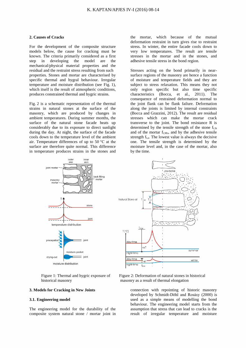
2. Causes of Cracks
For the development of the composite structure
models below, the cause for cracking must be
known. The criteria primarily considered as a first
step in developing the model are the
mechanical/physical material properties and the
residual and the restraint stress resulting from such
properties. Stones and mortar are characterised by
specific thermal and hygral behaviour. Irregular
temperature and moisture distribution (see Fig. 1),
which itself is the result of atmospheric conditions,
produces constrained thermal and hygric strains.
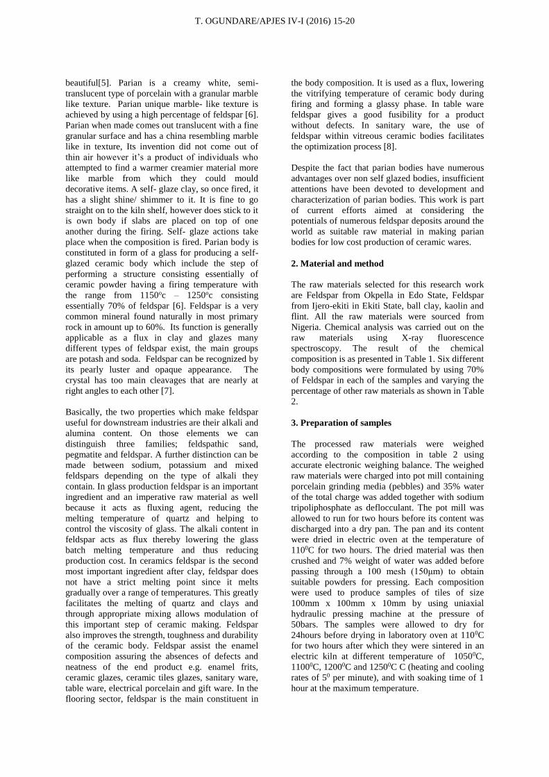
Fig. 2 is a schematic representation of the thermal
strains in natural stones at the surface of the
masonry, which are produced by changes in
ambient temperatures. During summer months, the
surface of the natural stone facade heats up
considerably due to its exposure to direct sunlight
during the day. At night, the surface of the facade
cools down to the temperature level of the ambient
air. Temperature differences of up to 50 °C at the
surface are therefore quite normal. This difference
in temperature produces strains in the stones and
the mortar, which because of the mutual
deformation restraint in turn gives rise to restraint
stress. In winter, the entire facade cools down to
very low temperatures. The result are tensile
stresses in the mortar and in the stones, and
adhesive tensile stress in the bond region.
Stresses acting on the bond primarily in near-
surface regions of the masonry are hence a function
of moisture and temperature fields and they are
subject to stress relaxation. This means they not
only region specific but also time specific
characteristics (Bocca, et al., 2011). The
consequence of restrained deformation normal to
the joint flank can be flank failure. Deformation
along the joints is limited by internal constraints
(Bocca and Grazzini, 2012). The result are residual
stresses which can make the mortar crack
transverse to the joint. The bond resistance R is
determined by the tensile strength of the stone ft,St
and of the mortar ft,Mo, and by the adhesive tensile
strength ft,a. The lowest value is always the decisive
one. The tensile strength is determined by the
moisture level and, in the case of the mortar, also
by the time.
Figure 1: Thermal and hygric exposure of
historical masonry
Figure 2: Deformation of natural stones in historical
masonry as a result of thermal elongation
3. Models for Cracking in New Joints
3.1. Engineering model
The engineering model for the durability of the
composite system natural stone / mortar joint in
connection with repointing of historic masonry
developed by Schmidt-Döhl and Rosásy (2000) is
used as a simple means of modelling the bond
behaviour. The engineering model starts from the
assumption that stress that can lead to cracks is the
result of irregular temperature and moisture

K. KAPTAN/APJES IV-I (2016) 08-14
distribution across the masonry cross section.
Thermal and hygral strain at the surface is
restrained by the inner masonry structure. The basic
function of the model is to calculate stresses at the
surface, starting from the simplifying assumption of
a fully constrained composite stone / mortar
element and maximum temperature difference:
0, CplelST (1)
(where T = Thermal strain, S = Shrinkage strain,
el,pl = Elastic-plastic strain and C = Creep strain)
Under conditions of full constraint, the sum total of
all strain components has to be 0 at the surface. For
the cases flank cracking (crack in parallel with the
joint, Fig. 3) and mortar cracking (crack normal to
the longitudinal direction of the joint, Fig. 4) the
different strain components are examined more
closely.
Figure 3: Cracking
parallel to joint
Figure 4: Cracking
normal to the joint
3.2. Crack initiation parallel to joint (side
cracks)
Thermal strain T is calculated with the aid of the
coefficient of thermal expansion T of mortar and
stone, the maximum temperature difference Tmax
occurring between mortar and stone or the
constraining action of the inside of the masonry (cf.
Figs. 1 and 2), and the percentage of area l0 taken
up by mortar and stone:
)1( ,0max,,,0max,, MoStStTMoMoMoTT lTlT
(2)
Shrinkage strain S is calculated with the aid of the
final degree of shrinkage S, of mortar and stone,
and the area percentage l0 of mortar and stone
(Collepardi, 1990). The final degree of shrinkage is
used for simplification, because it is expected that
the relative moisture in the mortar and stone
surfaces decisive for cracking will very quickly
follow any changes in the relative moisture of the
ambient air and that the constraint-induced
shrinkage strain will be produced at the surface:
)1( ,0,,,0,, MoStSMoMoSS ll (3)
Elastic-plastic strain el,pl is the result of the actual
stress t and the secant modulus Esec of mortar and
stone, and of the area percentage l0 of mortar and
stone in the composite stone / mortar system.
Respecting flank failure, the model starts from
series arranged mortar and stone:
St
Mo
MoMo
Mo
tplel
E
Ell
E
sec,
sec,
,0,0
sec,,
)1(
(4)
))1(
(,0,,0,
st
Mostt
Mo
MoMot
tCE
lC
E
lC
(5)
Creep strain C is calculated from the actual stress
t, the creep coefficients Ct of mortar and stone, the
modulus of elasticity E of mortar and stone, as well
as the area percentage l0 of mortar and stone
(Alberto, et al., 2011). Plugging equations 2 to 5
into eq. 1 and solving the equation for the
maximum stress the composite stone / mortar
system can take, or for the modulus of elasticity of
the mortar, yields equations 6 and 7:
StStSttMoMoMot
Mo
StMoStMo
StSStStTStMoSMoTMo
t
ElCElCE
EEll
TlTl
///1
)()(
,0,,0,
sec,
sec,sec,,0,0
,,max,,,0,,max,,0
(6)
MöMötMö
StStStStStt
t
StSStStTStMoSMoMoTMo
Mö
lCl
ElElCTlTl
E
,0,,0
sec,,0,0,
,,max,,,0,,max,,,0//
)()((
1
(7)
3.3. Crack initiation normal to joint (mortar
cracks)
The risk of crack propagation perpendicular to the
joint is assessed by connecting mortar and stones in
parallel rather than in series. When compared with
the residual stress in the mortar, the influence of the
stones on crack propagation in the mortar is
insignificant. This is why in this case the
engineering model is restricted to the mortar and
does not consider a composite stone / mortar
system. Again, considerations start from a fully
restrained system and the maximum temperature
difference.
The thermal strain is calculated with the aid of the
thermal coefficient of expansion T of the mortar
and the maximum difference in temperature Tmax
between mortar and the restraining masonry:
MoMoTT Tmax,, (8)
MoSS ,, (9)

K. KAPTAN/APJES IV-I (2016) 08-14
The shrinkage strain corresponds to the relevant
final degree of shrinkage S, of the mortar.The
elastic-plastic strain follows from the actual stress
t and the secant modulus Esec of the mortar
Mo
tplel
Esec,
,
(10)
Mo
Mott
CE
C ,
(11)
The creep strain C can be calculated from the
actual stress t, the creep coefficient Ct of the
mortar, and the modulus of elasticity E of the
mortar. Plugging equations 8 to 11 into eq. 1 and
solving the equation for the maximum stress the
mortar can take, or for the modulus of elasticity of
the mortar, yields equations 12 and 13.
Mot
MoSMoMoT
MotC
TE
,
,,max,,
1
(12)
MoSMoMoT
Mott
MoT
CE
,,max,,
, )1(
(13)
3.4. Implementation and application of the
engineering model
Equations 6 and 7, as well as 12 and 13, form the
basis for the engineering model which is applied in
the form of a Microsoft Access® database.
Respecting the variables in equations 2 to 5 and 8 to
11 the following distinctions can be made:
1. Parameters established on the structure :
Area percentage of mortar and stone
2. Parameters established experimentally or from
databases
coefficient of thermal expansion T of
mortar and stone
final degree of shrinkage S, of mortar
and stone
maximum temperature differences T
between mortar and stone
creep coefficients Ct of mortar and stone
modulus of elasticity of stone
Should these parameters not be established
experimentally, they can be assessed with the aid of
the engineering model or they can be imported from
the data records in the database.
3. Values established with the engineering model
and serving as a basis for mortar selection
stress t normal and perpendicular to the
joint flank
modulus of elasticity EMo of the mortar.
Stress t must not be greater than the strength of the
mortar, the strength of the stone or the bond
strength.
It has been developed a graphical user interface
using mortar and stone data available from
literature and data compiled from our own
investigations and analyses. This database can be
used for rough parameter studies to be able to select
mortars that promise to be a good choice for a given
masonry, and it can alternatively be used to
determine the requirements the intended mortar has
to meet. For verification of the model, the cracking
behaviour in the region of the joint of restrained
two-stone bodies was examined for constant
climatic conditions and for one-sided weather
exposure (Schmidt-Döhl and Rosásy 2000).A total
of three test series were run, all of them using
dolomite rock from the Harz mountains and green
sandstone from Rüthen as natural stone, and mortar
based on granulated blast-furnace slag and gypsum.
Stone and joint deformations, and deformations
beyond the joint were measured continuously, as
were the temperatures in the joint mortar. The
cracking behaviour was assessed weekly, and the
moisture content of mortar and stone was
determined gravimetrically once at the end of each
test series. Changes in the mortar temperature were
in addition measured at five points of a masonry
section at depths of approx. 2.5, 5, 10, 35 and
60 centimetres.
Even though the model only starts from linear-
elastic material behaviour (while considering time-
specific deformation), experimentally determined
results could be shown with a high degree of
approximation. But the accuracy of the model is
limited. Because it has so far been formulated as a
deterministic model, it does, for instance, not
account for the considerable variation of properties
of natural stone (Fassina, et al., 2002). Much
thought is at the moment being given to the
possibility of automated parameter studies. These
would also account for the variation in the mortar
and stone properties, provided they have been
stored in the database. Another aspect which is at
the moment not included in the calculation is the
bond shear strength, which is why shear stress
perpendicular to the crack front is not accounted
for. Neither does the model at the moment consider
any chemical degradation processes and frost-
induced processes, such as the degradation of
mortar properties as a result of weathering.

K. KAPTAN/APJES IV-I (2016) 08-14
Figure 5. Calculated Results of Flank Cracking of Three Different Gypsum-Lime-Mortars (R) and Two Different
Bricks (SLB = sand-lime brick – CB = clay brick)
Fig. 5 shows the results of comparative calculations
using the engineering model for flank failure under
temperature load case ΔT=5K. In this case, the
bond between three different gypsum-lime mortars
and calcareous sandstone or highly absorbent bricks
is considered (Twelmeier, et al., 2008). Once the
maximum stresses exceed the measured bond
strength, the flanks will fail. It is evident that the
stress-reducing effect of the creep deformation of
gypsum mortar has been considered in a very
realistic manner. Masonry samples exposed to this
temperature load case showed flank failure in the
same specimens as had been forecast in the model.
3.5. Research model
For the time being no model is available that would
be able to describe both heat and moisture
transport, and the complex material behaviour of
masonry (shrinkage, thermal strain, creep,
relaxation, failure patterns) with a high degree of
precision. One reason is the highly complex
dependence of the material behaviour on moisture
and temperature. This dependence pattern produces
coupled differential equations that have so far not
been solved satisfactorily with the FEM method
(Van Zijl 2000).
Up to the point at which cracking starts, hygral and
thermal transport can be assumed to be a process
that is independent of the mechanical condition of
the system. This is why a model has been
developed which combines the detailed sub-models
(Sperbeck 2004). Transport processes are calculated
with a program based on the finite-difference
method (FDM). This also provides for realistic
determination of transport processes under real
climatic conditions, including the effects of solar
radiation and driving rain. Results of the time-
specific thermal and moisture fields are transmitted
to an FEM program, which uses the material
models of Rots (1997), Lourenço (1996) and Van
Zijl (2000) to calculate the resultant deformations,
stresses, and cracking, due regard being given to
viscous and plastic material behaviour.
Figure 6. Geometric model and deformation conditions in
the research model
Figure 7. Two-dimensional illustration for the
wall cross section / Utilization of symmetries

K. KAPTAN/APJES IV-I (2016) 08-14
The research model is to serve as a basis for
extensive and effective analyses before starting
rehabilitation measures, while allowing the number
of pre-rehabilitation tests to be reduced
substantially. Quantitative determination of the
deformation and stress components, sensitivity
analyses etc. give more detailed insight into the
possible cause of cracks. The research model also
permits the moisture distribution to be assessed for
the entire cross section as a function of time. So far,
the model has been used to describe two-stone
bodies (see Fig. 6), in which heat and moisture
transport processes were still simulated separately
by making use of the symmetry (see Fig. 7).
Figs. 8 and 9 show the results of moisture
distribution, stress distribution and deformations for
a two-stone body when dried for 100 days (initial
situation: masonry with 90 % rel. air humidity; air
with 50 % rel. air humidity). The expected cracking
pattern as a result of the high dryness could be
approximated with a high degree of precision,
which is what measurements during test
programmes cannot achieve. Another advantage is
that climatic conditions can be simulated at random
and that the numerical model can be used for
probabilistic analyses. In this way it can also be
determined under what conditions the bond
between mortar and stone is particularly likely to
fail.
Figure 8. Moisture content and deformation
pattern across the cross section
Figure 9. Detail stone-joint: resulting stress in y-
direction and deformation pattern
4. Conclusions
The simple engineering model offers a tool that
permits the likelihood of cracks in new joints to be
assessed in a realistic manner. There is good
agreement between the results calculated with the
engineering model and the results of experimental
tests. On the whole, the cracking pattern was
forecast correctly. First coupled calculations using
the more complex research model also produce
plausible results. Model development aims at
providing an instrument that permits a better
understanding of the failure mechanisms in the
bond between natural stone and mortar joint. More
broadly based experiments are essential for
verification of both models.
5. References
[1] Alberto A., Antonaci P., Valente S. 2011.
Damage analysis of brick-to-mortar interfaces. In
Proceedings of 11th International Conference on
the Mechanical Behavior of Materials, 1151-1156,
Como Lake (Italy).
[2] Bocca P., Grazzini A., Masera D., Alberto
A.,Valente S. 2011. Mechanical interaction
between historical brick and repair mortar:
experimental and numerical tests. Journal of
Physics, 305, 1-10.
[3] Bocca P., Grazzini A. 2012. Experimental
procedure for the pre-qualification of strengthneing
mortars. International Journal of Architectural
Heritage, 6 (3): 302-321.
[4] Collepardi M. 1990. Degradation and
restoration of masonry walls of historical buildings.
Materials and Strctures, 23: 81-102.
[5] Fassina V., Favaro M., Naccari A. and Pigo M.
2002. Evaluation of compatibility and durability of
a hydraulic lime-based plaster applied on brick wall
masonry of historical buildings affected by rising
damp phenomena. Journal of Cultural Heritage, 3:
45-51.
[6] Grazzini, A. 2006. Experimental techniques for
the evaluation of the durability of strengthening

K. KAPTAN/APJES IV-I (2016) 08-14
works on historical masonry. Masonry
International, 19: 113-126.
[7] Lourenço, P. B. 1996. Dissertation.
Computational strategies for masonry strictures.
Delft University of Technology, Netherlands.
[8] Rots, J. G. 1997. Structural Masonry: An
Experimental/Numerical Basis for Practical Design
Rules., Rotterdam, Netherlands. Balkema.
[9] Schmidt-Döhl, F. and Rostàsy, F. S. 2000.
Abschlussbericht. Ingenieurmodell zur
Dauerhaftigkeit des Verbundsystems
Naturstein/Mörtelfuge mit Bezug auf die
Neuverfugung historischen Mauerwerks. iBMB,
TU Braunschweig.
[10] Twelmeier, H., Sperbeck, S. T., and
Budelmann, H. 2008. Restoration Mortar for
Historical Masonry – Durability Prediction by
means of numerical and Engineering Models, 14th
International Brick and Block Masonry Conference.
[11] Van Zijl, G.P.A.G. 2000. Computational
Modelling of Masonry Creep and Shrinkage.
Meinema BV, Delft, Netherlands.

T. OGUNDARE/APJES IV-I (2016) 15-20
*Corresponding author: Toluwalope OGUNDARE, Address: Department of Glass and Ceramic Technology Federal Polytechnic Ado Ekiti, Ekiti State, Nigeria, E-mail Address: [email protected], Phone:
2348038058132
Doi: 10.21541/apjes.08877
Development and Characterization of Parian Bodies Using Feldspar from
Two Selected Deposits in Nigeria
Toluwalope OGUNDARE1*, Oluwagbenga FATILE2 Olusola AJAYI,3 1,2,3Department of Glass and Ceramic Technology
Federal Polytechnic Ado Ekiti, Ekiti State, Nigeria
Geliş Tarihi: 2015-12-10 Kabul Tarihi: 2016-04-01
Abstract
Self glazed bodies also called Parian Bodies are chiefly composed of Feldspar which majorly acts as flux in
reducing the melting temperature of the particular ceramic body thereby reducing the stress of double firing a
ceramic product. In this present research work, Okpella and Ijero-Ekiti feldspar deposits in Nigeria together with
other raw materials were utilized to develop parian bodies which are very suitable for making ceramic tiles, dolls
and figurines. Chemical analyses were carried out on the raw materials using X-ray fluorescence (XRF) in order
to ascertain their suitability for developing parian bodies. Six compositions were made from these two deposits
using a standard parian body composition of 70% feldspar. The samples were shaped, dried and sintered between
1050 oC - 1250 oC at the interval of 500C. Flexural strength, fired shrinkage, porosity and water absorption tests
were used to characterize the samples. The results showed that samples fired at 12000C and 12500C exhibited
technological properties that meet up with ISO standards. The two feldspar deposits were found to be suitable for
developing parian bodies.
Keywords: Parian, Feldspar, Kaolin, Porcelain, Sintered, Whiteware.
1. Introduction
Recently, the development of self glazed porcelain
ware is attracting interest from researchers in
Ceramic Technology field owing to their
technological properties and low cost of production.
Porcelain bodies are usually made up of at least
three components that play the three fundamental
roles for optimum processing, and hence
performance of the final products, kaolin or
kaolinitic clay for plasticity, feldspar for fluxing
and silica as filler for the structure [1]. The thermal,
dielectric and mechanical properties of the products
can be improved by varying the proportions of the
three main ingredients [2]. The main differences
between compositions are in the relative amounts
and kinds of raw materials used. Most times, it is
observed that an increasing amount of feldspar
added to porcelain body composition usually results
in formation of liquid phase at the eutectic
temperature, which increases the degree of
vitrification and translucency at lower temperature
[3]. As feldspar is replaced by clay, higher
temperatures are required for vitrification due to the
introduction of a more refractory material, and the
firing process becomes more difficult and
expensive. However, the forming processes become
easier, and the mechanical properties of the
resulting body are improved [4]. Porcelain happens
to be a class of whiteware, which is distinguished
from the other class by its firing temperature,
composition and mainly by the lack of open
porosities on the fired body, but self glazing effect
can be achieved from porcelain bodies with
introduction of high quantity of fluxes. This self
glazing ceramic ware is known as “Parian” and has
been achieved by introducing certain fluxes like
feldspar which when fired at high temperatures
contributes to the formation of a thin layer of glass
fused at the ware surface. This glass film has a very
similar composition to the respective ceramic
material and prevents the hairline cracks known as
crazing. Parian is extremely translucent through a
large temperature range and ideally suited for
casting to produce figurines, dolls and light forms.
This body is chiefly made up of very white feldspar
which uses a floatation method of particles
distribution and some frothing may occur due to
high speed of mixing. Parian was a development of
earlier biscuit porcelain, but has higher proportion
of feldspar in body composition than the normal
porcelain, makers fired it at a lower temperature
and the high content of feldspar present in the body
will make the fired ware to be more vitrified, thus
possessing a colour verging on ivory and having a
marble like structure that is smoother than that of
biscuit or glazed ware. When parian bodies are
made, they come out faint but extremely
T. OGUNDARE/APJES IV-I (2016) 15-20
beautiful[5]. Parian is a creamy white, semi-
translucent type of porcelain with a granular marble
like texture. Parian unique marble- like texture is
achieved by using a high percentage of feldspar [6].
Parian when made comes out translucent with a fine
granular surface and has a china resembling marble
like in texture, Its invention did not come out of
thin air however it’s a product of individuals who
attempted to find a warmer creamier material more
like marble from which they could mould
decorative items. A self- glaze clay, so once fired, it
has a slight shine/ shimmer to it. It is fine to go
straight on to the kiln shelf, however does stick to it
is own body if slabs are placed on top of one
another during the firing. Self- glaze actions take
place when the composition is fired. Parian body is
constituted in form of a glass for producing a self-
glazed ceramic body which include the step of
performing a structure consisting essentially of
ceramic powder having a firing temperature with
the range from 1150oc – 1250oc consisting
essentially 70% of feldspar [6]. Feldspar is a very
common mineral found naturally in most primary
rock in amount up to 60%. Its function is generally
applicable as a flux in clay and glazes many
different types of feldspar exist, the main groups
are potash and soda. Feldspar can be recognized by
its pearly luster and opaque appearance. The
crystal has too main cleavages that are nearly at
right angles to each other [7].
Basically, the two properties which make feldspar
useful for downstream industries are their alkali and
alumina content. On those elements we can
distinguish three families; feldspathic sand,
pegmatite and feldspar. A further distinction can be
made between sodium, potassium and mixed
feldspars depending on the type of alkali they
contain. In glass production feldspar is an important
ingredient and an imperative raw material as well
because it acts as fluxing agent, reducing the
melting temperature of quartz and helping to
control the viscosity of glass. The alkali content in
feldspar acts as flux thereby lowering the glass
batch melting temperature and thus reducing
production cost. In ceramics feldspar is the second
most important ingredient after clay, feldspar does
not have a strict melting point since it melts
gradually over a range of temperatures. This greatly
facilitates the melting of quartz and clays and
through appropriate mixing allows modulation of
this important step of ceramic making. Feldspar
also improves the strength, toughness and durability
of the ceramic body. Feldspar assist the enamel
composition assuring the absences of defects and
neatness of the end product e.g. enamel frits,
ceramic glazes, ceramic tiles glazes, sanitary ware,
table ware, electrical porcelain and gift ware. In the
flooring sector, feldspar is the main constituent in
the body composition. It is used as a flux, lowering
the vitrifying temperature of ceramic body during
firing and forming a glassy phase. In table ware
feldspar gives a good fusibility for a product
without defects. In sanitary ware, the use of
feldspar within vitreous ceramic bodies facilitates
the optimization process [8].
Despite the fact that parian bodies have numerous
advantages over non self glazed bodies, insufficient
attentions have been devoted to development and
characterization of parian bodies. This work is part
of current efforts aimed at considering the
potentials of numerous feldspar deposits around the
world as suitable raw material in making parian
bodies for low cost production of ceramic wares.
2. Material and method
The raw materials selected for this research work
are Feldspar from Okpella in Edo State, Feldspar
from Ijero-ekiti in Ekiti State, ball clay, kaolin and
flint. All the raw materials were sourced from
Nigeria. Chemical analysis was carried out on the
raw materials using X-ray fluorescence
spectroscopy. The result of the chemical
composition is as presented in Table 1. Six different
body compositions were formulated by using 70%
of Feldspar in each of the samples and varying the
percentage of other raw materials as shown in Table
2.
3. Preparation of samples
The processed raw materials were weighed
according to the composition in table 2 using
accurate electronic weighing balance. The weighed
raw materials were charged into pot mill containing
porcelain grinding media (pebbles) and 35% water
of the total charge was added together with sodium
tripoliphosphate as deflocculant. The pot mill was
allowed to run for two hours before its content was
discharged into a dry pan. The pan and its content
were dried in electric oven at the temperature of
1100C for two hours. The dried material was then
crushed and 7% weight of water was added before
passing through a 100 mesh (150μm) to obtain
suitable powders for pressing. Each composition
were used to produce samples of tiles of size
100mm x 100mm x 10mm by using uniaxial
hydraulic pressing machine at the pressure of
50bars. The samples were allowed to dry for
24hours before drying in laboratory oven at 1100C
for two hours after which they were sintered in an
electric kiln at different temperature of 10500C,
11000C, 12000C and 12500C C (heating and cooling
rates of 50 per minute), and with soaking time of 1
hour at the maximum temperature.

T. OGUNDARE/APJES IV-I (2016) 15-20
4. Characterization of the samples
The samples produced were characterized using
standard methods in order to determine their
technical properties. The shrinkage test was carried
out on the samples by determining the initial length
before firing (Lo) and the length after firing (Lf)
using digital venier caliper. The Percentage linear
shrinkage was determined using equation (1).
% 𝐿𝑖𝑛𝑒𝑎𝑟 𝑆ℎ𝑟𝑖𝑛𝑘𝑎𝑔𝑒 =Lo – Lf
Lo x 100 (1)
Table 1: Chemical Composition of Raw Materials (wt. %)
Material Oxides (wt. %)
SiO2 Al2O3 CaO Na2O Fe2O3 K2O MgO MnO LOI
Ijero
Feldspar
66.47 18.20 0.65 2.84 0.33 9.61 0.25 - -
Okpella
Feldspar
65.98 14.62 0.95 3.62 0.76 8.87 0.29 - -
Kaolin 48.21 33.36 0.23 0.13 0.74 0.77 0.05 - 12.83
Quartz 96.12 1.17 0.11 0.62 0.12 0.20 0.07 - 3.84
Ball Clay 44.82 37.35 0.07 0.11 1.09 0.89 0.12 - -
Table 2: Formulation of the Samples (Wt. %)
Okpella Feldspar Ijero Feldspar Flint Kaolin Ball Clay
A 70 30
B 70 10 20
C 70 10 20
D 70 30
E 70 10 20
F 70 10 20
The flexural strength was determined using a
universal testing machine (MTS 810.23M), in
three-point bending fixture, 70 mm support span
and with a crosshead speed of s0.5mm min-1.
Porosity and water absorption were determined
using boiling method.The specimen were subjected
to 1 hour boiling followed by an additional two
hour water soaking and then weighed as Wsat .The
soaked specimen were then suspended from the
beam of a balance in a vessel of water in such a
way that specimen were completely immersed in
the water without touching the side of the vessel.
Weights of the suspended specimen were
determined as Wsus. The specimen were dried in
oven for 24hours and the weight were determined
as Wd. The test was carried out on four
representative specimens. Percentage porosity and
water absorption were calculated using equation 2
and equation 3 respectively.
𝑃𝑜𝑟𝑜𝑠𝑖𝑡𝑦 =Wsat− Wd
Wsat− Wsus x 100 (2)
𝑊𝑎𝑡𝑒𝑟 𝑎𝑏𝑠𝑜𝑟𝑝𝑡𝑖𝑜𝑛 =Wsat− Wd
Wd x 100 (3)
5. Results and discussion
Result of the linear shrinkages after firing at
different temperatures is as presented in figure
1.The linear shrinkage indicates the degree of
densification during firing, and it is very important
for the dimensional control of the ceramic products.
It is observed from figure 1 that linear shrinkage
values of the samples were within the range of
2.4%-10.4%. These values are within the safe limits
for industrial production of self glazed porcelain
products. Generally, it is observed that the linear
shrinkage of the samples increased with increase in
temperature with samples sintered at 12000C
exhibiting the highest linear shrinkage with the
exception of sample A and F. It is also observed
that sample C exhibited the highest linear shrinkage
at all temperatures in comparison with other
samples.
Figure 2 also shows the results of water absorption
tests carried out on the samples. From figure 2, it is
observed that the water absorption generally
decreased with increase in firing temperature with
samples fired at 12500C exhibiting the lowest water
absorption values. The decrease in water absorption
values at high temperature could be attributed to the
formation of more liquid phase that mainly
originated from the feldspar. The liquid phase aids
sintering which resulted in maximum vitrification at
high temperature. This behaviour is similar to that
showed by nearly all porcelain bodies [2].
All the samples fired at 12000C and 12500C had
water absorption values within the range of 0.1%-

T. OGUNDARE/APJES IV-I (2016) 15-20
0.5%.This implies that all the samples fired at
12000C and 12500C meet up with ISO standard
which recommended water absorption value of not
greater than 0.5% for porcelain tiles. The result is
also in agreement with previous work reported by
other authors [1, 9].
Figure 1. Linear shrinkage of samples sintered at different temperature
Figure 2. Water absorption of samples sintered at different temperature
0
2
4
6
8
10
12
A B C D E F
Lin
ear
Sh
rin
kage
(%
)
Sample Designation
1050 oC
1100 oC
1200 oC
1250 oC
0
0,5
1
1,5
2
2,5
3
3,5
4
A B C D E F
Wat
er
Ab
sorp
tio
n (
%)
Sample Designation
1050 oC
1100 oC
1200 oC
1250 oC

T. OGUNDARE/APJES IV-I (2016) 15-20
Figure 3. Porosity of samples sintered at different temperature
Figure 4. Flexural strength of samples sintered at different temperature
The result of porosity tests carried out on the
samples is as presented in figure 3. Porosity of the
fired samples is associated to other properties such
as water absorption and linear shrinkage. The result
followed the same trend with that of water
absorption rate. From figure 3, it is generally
observed that the percentage porosity value of the
samples decreased with increase in sintering
temperature. Martin-Marquez et al [10] have
reported that optimum vitrification range is
achieved in porcelain tiles when open porosity
reaches a minimum value, tending to be nearly
zero, and simultaneously linear shrinkage is
maximum.
0
2
4
6
8
10
12
14
16
18
A B C D E F
Po
rosi
ty (
%)
Sample Designation
1050 oC
1100 oC
1200 oC
1250 oC
0
10
20
30
40
50
60
A B C D E F
Fle
xura
l Str
en
gth
(M
Pa)
Sample Designation
1050 oC
1100 oC
1200 oC
1250 oC
T. OGUNDARE/APJES IV-I (2016) 15-20
The result of bending strength test of the samples
sintered between 10500C and 12500C is as
presented in figure 4. The result shows that the
flexural strength values of the samples are within
the range of 20.4Mpa-53.4Mpa. From figure 4, it is
generally observed that the flexural strength of the
samples increased with increase in firing
temperature with sample C exhibiting the highest
flexural strength values at all temperature in
comparison with other samples. The high flexural
strength values exhibited by sample C at all
temperature are also consistence with the water
absorption values. Boussak et al. [11] have reported
that increase in temperature of ceramic
compositions containing clays and feldspars result
in higher mullite formation, thereby improving
mechanical properties.
Although, sample C and F contained 70% of
Okpella feldspar and Ijero feldspar respectively but
chemical analyses of the two feldspar samples
showed Okpella feldspar contains more fluxes in
comparison with Ijero feldspar. The higher
percentage of fluxes in Okpella feldspar contributed
to formation of more liquid phase in sample C
which enhanced its vitrification and flexural
strength in comparison with sample F. According to
ISO standard, the minimum flexural strength value
recommended for porcelain tiles is 35Mpa. This
implies that nearly all the samples fired at 12000C
and 12500C meet up with ISO standard with the
exemption of sample A and D fired at 12000C.
6. Conclusions
The development and characterization of parian
body using feldspar from two selected deposits in
Nigeria was successfully investigated. The results
show that:
The percentage linear shrinkage of the
samples increased with increase in firing
temperature with sample C exhibiting the
highest linear shrinkage.
All the samples fired at 12000C and
12500C had water absorption values of not
greater than 0.5% which is the required
standard for porcelain tiles according to
ISO.
All the samples fired at 12000C and
12500C had flexural strength values of not
less than 35Mpa with the exemption of
sample A and D.
Sample C and F fired at 12000C and
12500C produced the best self glazed body
which also meet up with require standards.
7. References
[1] Kamseu E., Leonelli C., Boccaccini D.N.,
Veronesi P., Miselli P., Giancarlo P. and Chinje
M.U., Characterisation of Porcelain Compositions
Using Two China Clays from Cameroon, Ceramics
International, 2007, 33, p. 851-857.
[2] Peter W.O., Stefan J. and Joseph K.B.,
Characterization of Feldspar and Quartz Raw
Materials in Uganda for Manufacture of Electrical
Porcelains, Journal of Australia Ceramic Society,
2006, 41(1), p. 29-35.
[3] Reed, J.S., Principles of Ceramics Processing,
New York, Wiley & Sons, 1995.
[4]McLaren E. A. and Cao P. T. Ceramics in
Dentistry—Part I: Classes of Materials. Inside
Dentistry; 2009.
[5] Carty, W.M., 2002, Observation on the Glass
Phase Composition in Porcelains. Chem. Eng. Sci.
Proc., 2002, 23(2), p. 79-94.
[6] Holdren, G.R and Berner, R.A, Mechanism of
Feldspar Weathering.
low Temperature Feldspars in Sedimentary Rocks,
American Journal of Science, 1999, p. 279, 435-
479.
[7] Ima (2000). Ceramic Raw Materials. London
Pergarmon Press.
[8] Nelson,I and Stephen, A (2008): Weathering
and Clays minerals.
[9] Matthew G.O., and Fatile B.O.,
Characterization of Vitrified Porcelain Tiles Using
Feldspar from Three Selected Deposits in Nigeria.
Research Journal of Recent Sciences, 2014, 3(9), p.
67-72.
[10] Martín-Márquez J., Rincón M.J. and Romero
M., Effect of firing temperature on sintering of
porcelain stoneware tiles, Ceramics Internacional,
2008, 34, p. 1867-1873.
[11] Boussak H., Chemani H., and Serier A.,
Characterization of Porcelain Tableware
Formulation Containing Bentonite Clay,
International Journal of Physical Sciences, 2014,
10(1), p. 38-45.

A.O. FATOYE/APJES IV-I (2016) 21-27
*Corresponding author: Department of Chemistry, Federal University of Technology, Akure, Ondo State, Nigeria,
E- mail: [email protected], Phone: +2348036605518
Doi:10.21541/apjes.61578
Fractional Distribution of Heavy Metals from the Tailings of Itagunmodi
Goldmine Site Osun State, Nigeria
Abiodun O. FATOYE1,2* and Albert. O ADEBAYO1 1*Department of Chemistry, Federal University of Technology, Akure, Ondo State, Nigeria.
2Department of Science Technology, Federal Polytechnic Ado Ekiti, Ekiti State, Nigeria.
Geliş Tarihi: 2015-11-19 Kabul Tarihi: 22.03.2016
Abstract
The distribution of heavy metals (Cu, Ni, Cd, Cr, Zn and Fe) in goldmine tailing was determined using multi- step
sequential extraction. Chemical properties such as pH, conductivity, cation exchange capacity, organic matter,
residual humidity and particle size were also analyzed. Similar characteristics distribution patterns were observed for
Cd, Cr, Fe and Zn except Cu. The percentage recovery of Ni ranged from 95.25-99.24%. The high Mobility factor
and bioaccumulation factor values of soil Ni may be interpreted as symptoms of relatively high liability and
biological availability of the metals in soil.
Keywords: Tailings, Heavy Metals, Goldmine, Sequential Extraction, Distribution
1. Introduction
Mining gives rise to soil erosion and environmental
contamination by generating waste during the
extraction, beneficiation, and processing of minerals.
After closure, mines can still impact the environment
by contaminating air, water, soil, and wetland
sediments from the scattered tailings, as well as
pollution of groundwater by discharged leachate,
unless the proper remediation is conducted [1].
Mining activities contribute to heavy metal pollution
of the environment [2,3]. Progressive accumulation
of heavy metals in soils surrounded by mines, result
in increased heavy metal uptake by plants. This is
worrisome because of potential health risk to the
people leaving in the surrounding areas [4].
Elements like Cd, Cr and Ni, are said to be non
biodegradable thus, persist everywhere in the
environment and have the ability to be deposited in
various body organs which poses a great threat to the
human health. Several studies have shown that plants,
growing in heavy metal contaminated soils have
higher concentrations of heavy metals than those
grown in uncontaminated soil [5]. It has been
reported that serious health problems may develop as
a result of excessive accumulation of heavy metals
such as Cd, and Pb in the human body [6]. Despite
Zn and Cu being essential elements in the diet, high
concentration in plants is of great concern because
they are toxic to humans and animals [7]. Pb and Cd
metals are believed to be potential carcinogens and
are implicated in the ontology of many diseases,
especially cardiovascular diseases, kidney, nervous
system, blood as well as bone ailments [8].
Heavy metal contamination of agricultural soils and
crops surrounding the mining areas is a serious
environmental problem in many countries, Nigeria
inclusive [9].
It is well known that metals in soil are presented in
different chemical forms, which influence their
reactivity and hence their mobility and
bioavailability. Evaluating metal pollution of soils on
the basis of total metal content provides little
information on the mobility and bioavailability of
heavy metals and thus gives poor guidance for the
selection of appropriate remediation strategies for
contaminated soil.
Recently, pollution of general environment has
increasingly gathered a global interest. In this respect,
contamination of agricultural soils with heavy metals
has always been considered a critical challenge in
scientific community [10].

A.O. FATOYE/APJES IV-I (2016) 21-27
A sequential chemical extraction technique
fractionates heavy metals into forms of different
solubilities and mobilities, and can therefore furnish
potential valuable information for predicting metal
availability and metal movement in the soil.
Speciation of metals in soils, sediments and solid
wastes is often studied using sequential extraction
techniques whereby the target metals are fractionated
into several fractions using extractant solutions of
increasing strength [11] Several such sequential
extraction schemes have been described [11,12]. The
technique has been used to study the speciation of
heavy metals in soils, street sweepings and urban
aquatic sediments, lake sediments, pelagic sediments,
semiarid soils, dredged sediment derived surface
soils, and solid waste materials [12]. The technique
has also been used to study the speciation, mobility
and bioavailability of radionuclides [13,14,15]. It is
very important to evaluate the mine tailing to actually
ascertain the distribution of the heavy metals which is
the focus of the research.
2. Material and Method
Itagunmodi is a small community lies between
latitudes 7°30’ and 7°33’ N and between longitudes
4°36’ and 4°39’ E in Atakumosa West Local
Government Council southwestern Nigeria (Figure
1). The study area as shown in the map below is a
rural community of about 2,400 to 2,600 people that
engage predominantly in subsistence farming and
cocoa plantation. Itagunmodi is a community with
many dilapidated buildings.
Figure 1. A map is belonging to Itagunmodi
Tailings samples were oven dried at 400C for two
weeks. Samples were sieved through a 0.8mm mesh
and stored in clean polythene bags for further
analysis.
The pH was determined by the method [16], particle
size analysis by (hydrometer meter), conductivity by
(conductivity meter), CEC by ammonium acetate
method [17], Organic matter content [18], Residual
humidity [19].
Dried and powdered soil sample of 1.2 g was
digested with aqua regia (3:1 HCl: HNO3) in 100 ml
conical flask on a hotplate and diluted to volume with
distilled water. Fe, Cr, Cu, Zn, Cd, and Ni in the
digest were determined using 210 VGP (Buck
Scientific) atomic absorption spectrophotometer. The
detection limit of the atomic absorption
spectrophotometer used is 0.01.
The sequential extraction of metals was done by the
method of Tessier et al,1979 which partitions metals
into exchangeable, bound to carbonates, bound to Fe
– Mn Oxides, bound to organic matter and residual.
1g of air dried tailing sample were used.

A.O. FATOYE/APJES IV-I (2016) 21-27
Table 1. Testing parameters
Fraction Extractant Shaking Time(hr) Temp(oC) Designation
F1 1M MgCl2,pH 7 1 RM Exchangeable
F2 1M NaAC, pH 5 5 RM Carbonate
F3 0.04M
NH2(OH)Cl/25%CH3COOH
5 96 Fe-Mn oxide
F4 0.02M HNO3/30%H2O2, pH2 5 85 0rganic/Sulphide
F5 HClO4/HF Residual
Source : Tessier et al, (1979).
Validation of the analytical results was tested by
recovery experiments because there was no standard
reference material (SRM), which is more preferential
or needed to control the accuracy of the method
studied, in our laboratory. An important consideration
in the reliability of a sequential extraction data is the
percentage recovery relative to a single digestion
using a mixture of strong mineral acids or generally a
mixture of strong acids at the digestion of the residual
phase of the sequential extraction protocol employed
[20]. Recovery is defined as follows:
R= X100
F is the different fractions while SDSA is the single
digestion for single acid
The distribution of heavy metals in the sample allows
us to predict their mobility and bioavailability. The
bioavailability factor was expressed as the ratio of the
available concentration of a metal in soil to its total
concentration. It shows the potentials of a particular
metal from the soil matrix to enter the soil solution
from which it can be absorbed by plants. Mobility
factor was expressed as percentage of the
Bioavailability factor
3. Results
Table 2. Showing the result of physicochemical characteristics of tailing samples
Av: Average, Ran: Range
P value=0.834, then P>0.05, there is no significant difference (ANOVA & DUNCAN)
EC= Electrical conductivity, CEC= Cation exchange capacity, OC= Organic carbon, OM= Organic matter, RH=
Residual humidity
pH EC
(uS/cm)
CEC
(Meq/100g)
OC
(%)
OM
(%)
RH
(%)
Sand
(%)
Clay
(%)
Silt
(%)
Texture
1 4.27±0.77 66.0±6.50 3.16±5.35 0.45±1.13 0.78±1.97 0.30±0.02 75.0±4.30 18.0±5.80 7.0±4.20 Sand
2 4.30±0.77 70.0±6.50 2.30±5.35 0.72±1.13 1.25±1.97 0.22±0.02 78.0±4.30 5.0±5.80 17.0±7.40 Loamy
Sand
3 4.84±0.77 75.0±6.5 3.06±5.35 0.35±1.13 0.60±1.97 0.20±0.02 74.0±4.30 3.0±5.80 23.0±7.40 Loamy
Sand
4 5.61±0.77 79.0±6.50 13.48±5.35 2.49±1.13 4.28±1.97 0.26±0.02 85.0±4.30 10.0±5.80 5.0±7.40 Sand
5 5.98±0.77 82.0±6.50 11.70±5.35 2.62±1.13 4.59±1.97 0.25±0.02 78.0±4.30 8.0±5.80 14.0±7.40 Loamy
Sand
Av. 5.0 78.4 6.74 1.33 2.30 0.246 - - - -
Ran 4.27-5.98 66-95 2.30-13.48 0.35-2.62 0.60-4.59 0.20-0.30 - - - -

A.O. FATOYE/APJES IV-I (2016) 21-27
Table 3. Concentration of Tailing Cu in individual Fractions (mg/kg)
Loc F1 F2 F3 F4 F5 Total Cu in
original
Sample
%Recovery %BF %MF
1 0.00a,b 1.00a±0.35 0.00a 6.00a±0.20 36.0b±0.20 43.0 48.13 99.69 0.023 2.3
2 0.00a,b 2.00a±0.20 0.00a 0.00a 28.0b±0.20 30.0 30.71 97.68 0.07 7.0
3 0.00a,b 0.00a 0.00a 0.00a 30.0b±0.10 30.0 31.80 94.38 0.00 0
4 0.00a,b 1.00a±0.35 0.00a 0.50a±0.10 15.5b±0.20 17.0 18.05 94.18 0.06 6.0
5 0.50a,b±0.3 0.00a 0.00a 17.5a±0.20 45.0b±0.25 63.0 65.0 96.77 0.08 0.8
Value with different superscript on the same row are significant (p<0.05)
Table 4. Concentration of Tailing Ni in individual Fractions (mg/kg) Loc F1 F2 F3 F4 F5 Total Ni in
original
Sample
% Reco
very
%BF %MF
1 9.00 a±0.95 6.00 a±0.25 5.00a±0.10 1.00a±1.20 57.5 b±0.1 78.0 79.91 98.25 0.19 19
2 8.50 a±2.05 7.50 a±1.40 5.00 a±0.35 0.00 a 56.0 b±2.0 77.0 77.84 98.92 0.21 21
3 8.00 a±0.95 6.50 a±0.45 0.35 a±0.12 1.00 a1.0 68.15b±1.5 84.0 84.16 95.25 0.17 17
4 8.00 a±0.40 8.00 a±1.40 3.00 a±0.65 1.00 a±1.0 35.0 b±0.5 55.0 56.15 97.95 0.29 29
5 7.00 a±0.30 0.00a 0.00 a 17.50 a±0.20 45.0 b±3.2 55.50 91.69 60.53 0.13 13
Value with different superscript on the same row are significant (p<0.05)
Table 5. Concentration of Tailing Zn in individual Fractions (mg/kg) Loc F1 F2 F3 F4 F5 Total Zn in
original
Sample
%Reco
very
%BF %MF
1 7.50 a±0.65 11.50a±3.70 12.30a±4.15 9.00 a±2.25 28.0a±2.30 68.5 69.19 99.00 0.28 28
2 2.80 a±1.25 8.00 a±2.25 9.50 a±1.45 8.00 a±0.05 26.0a±2.00 54.5 55.87 97.55 0.19 19
3 2.00 a±1.65 7.00 a±1.65 8.50 a±1.50 9.50 a±2.00 27.0 a±1.00 54.0 55.30 97.65 0.17 17
4 6.00 a±0.55 7.50 a±1.25 12.0 a±2.35 11.5 a±1.30 6.00 a±0.50 43.0 44.18 97.33 0.31 31
5 1.00 a±0.30 38.0 a±0.80 39.5 a±0.20 32.5 a±1.10 31.0 a±4.45 141.5 142.91 99.00 0.28 28
Value with different superscript on the same row are significant (p<0.05)
Table 6. Concentration of Tailing Cr in individual Fractions (mg/kg) Loc F1 F2 F3 F4 F5 Tota
l
Cr in \
original
Sample
%Reco
very
%BF %MF
1 0.00 a 2.25 b±0.25 0.00 a 2.45 b±0.45 0.40 a±0.04 5.10 5.58 91.40 0.44 44
2 0.00 a 4.75 b±0.25 0.00 a 4.20 b±0.40 0.85 a±0.45 9.80 10.40 94.23 0.48 48
3 0.00 a 6.40 b±0.15 0.00 a 6.20 b±0.60 0.20 a±0.05 12.8 13.48 94.96 0.50 50
4 0.00 a 8.05 b±0.25 1.00 a±0.20 8.45 b±0.65 0.00 a 17.5 18.55 94.34 0.46 46
5 6.15a±0.65 0.00 b 1.85 a±0.20 8.20 b±0.05 0.15 a±0.50 16.35 17.46 93.64 0.38 38
Value with different superscript on the same row are significant (p<0.05)
Table 7. Concentration of Tailing Cd in individual Fractions (mg/kg) Loc F1 F2 F3 F4 F5 Total Cd in
original
Sample
%Reco
very
%BF %MF
1 0.00 a 0.25 a±0.05 0.25a±0.05 0.10 a±0.00 0.10a±0.05 0.85 1.54 55.19 0.29 29
2 1.10 a±0.50 0.50 a±0.20 0.35 ±0.05 0.05 a±0.05 0.00 a 0.20 2.17 92.17 0.80 80
3 0.50 a±0.10 0.30 a±0.10 0.15 ±0.10 0.85 a±0.05 0.40a±0.15 2.20 2.43 90.95 0.36 36
4 0.015a±0.00 0.25 a±0.00 0.30a±0.00 0.45 a±0.05 0.35a±0.10 1.37 1.49 91.95 0.19 19
5 0.25 a±0.05 0.30 a±0.05 0.50a±0.15 0.60 a±0.05 0.20a±0.05 1.85 2.00 92.50 0.30 30
Value with different superscript on the same row are significant (p<0.05)

A.O. FATOYE/APJES IV-I (2016) 21-27
Table 8. Concentration of Tailing Fe in individual Fractions (mg/kg) Loc F1 F2 F3 F4 F5 Total Fe in
original
Sample
%Recov
ery
%BF %MF
1 10.40a±0.50 392.15b±0.15 446.15d±0.35 345.95b,c±1.75 338.25c,d±0.20 1552.90 1554.31 100.09 0.26 26
2 5.50 a±0.05 164.90b±0.15 435.50d±0.30 182.80b,c±0.20 425.0 c,d±1.50 1213.70 1634.98 74.24 0.14 14
3 6.25 a±0.10 388.95b±0.40 441.80d±1.50 182.20b,c±1.35 472.0 c,d±0.10 1491.20 1506.20 99.0 0.27 27
4 6.80 a±0.60 16.25 b±0.15 477.25d±0.35 276.05b,c±1.55 476.0 c,d±1.00 1052.35 1057.55 99.51 0.022 2.2
5 4.95 a±0.10 51.15 b±0.05 484.75d±0.15 474.60b,c±1.60 486.5 c,d±0.10 1401.15 1412.15 99.28 0.040 4.0
Value with different superscript on the same row are significant (p<0.05)
4. Discussion
Physicochemical properties of the tailings was
conducted and the result is presented on Table 2. The
pH values of the tailing samples range from 4.27 to
5.98 with a mean value of 5.0 which shows that the
tailings are slightly acidic. Residual humidity range
from 0.20-0.30% with an average of 0.246. Since
residual humidity is proportional to the content of
clay and organic matter, tailing has low residual
humidity, it indicated less clay but range from loamy
sand to sand.. EC range from 66-95 µS/cm with a
mean value of 78.4 µS /cm. Furthermore, CEC
ranged from 2.30 to 13.48Meq/100g with a mean
value of 6.74Meq/100g. The percentage organic
carbon (%OC) ranged from 0.35 to 2.62 with a mean
value of 6.74. Also, percentage organic matter (%0N)
ranged from 0.60-4.59 with a mean value of 2.30.
Similar results are reported [1].
The sequential extraction procedures results provided
information on the potential mobility and
bioavailability of the studied elements in this
research. The distribution of heavy metals in the
sample allows us to predict their mobility and
bioavailability in the tailing. The bioavailability
factor was expressed as the ratio of the available
concentration of a metal in soil to its total
concentration. It shows the potentials of a particular
metal from the soil matrix to enter the soil solution
from which it can be absorbed by plants. Mobility
factor was expressed as percentage of the
Bioavailability factor. The speciation of the metals
are shown in Table 3-7 for their individual metals.
Cu was mainly presented in the residual fraction and
organic matter fraction as shown in Table 3. The
content of residual fraction ranged from 68%-91%
and varied in the range of 5%-27% in organic matter
fraction .the level of copper is exchangeable ,
carbonate fraction and fraction bond to hydrate oxide
of iron and manganese was lower. Copper is bound
much more tightly by organic matter than Ni and is
much less likely to be displaced by the
hydroxylamine hydrochloride reagent. Similar results
are reported by [21,22]. Copper in the soil is not
present in the ionic forms which reduce its toxicity.
Ni is mainly found in the fraction bound to residual
that it varies from 63%-81% as shown on Table 4.
Whereas 0%-27.7% in organic and sulfide fraction.
The level of Ni in other fraction is considerably low.
Toxicity of nickel is not important because of its low
concentration in the mobile and bio available
fractions.
Heavy metals in residual fraction are not likely to be
discharged under normal environment conditions. Ni
was mainly associated with residual fractions, so its
status in the soil was considered stable [22].
The analysis from Table 5 shows that Zn has been
bound to hydrated oxides of iron and manganese
fraction and varied in different sample in the range of
15.7%-27.9%. The amount of zinc found in the
carbonated fractions varies from 13%-26.9%.Similar
results are reported by [24].
Chromium in the tailings sample is mainly found in
the organic and sulfide metal fraction with an average
of 48% and little lesser in the range of 44%-46%
bound to carbonate. Whereas it is smaller in residual
ranges from 0%-8.7% as shown on Table 6.
Thus, the bioavailability of chromium in the tailing
sample is considered insignificant. It is low in
exchangeable and iron-manganese oxide metal bound
fraction.
The analysis of cadmium from Table 7 in different
soil samples have been found in organic and sulfide
metal fraction range from 2.5%-38.65% and varied in
the range of 6.8%-27% in iron manganese oxide
metal fraction. The level of cadmium in
exchangeable, carbonate bound, and residue fraction
was lower absorption by hydrated CaCO3 has been
shown to be reversible [23].

A.O. FATOYE/APJES IV-I (2016) 21-27
The results shows that iron occurred more in residual
fraction which is varied between 26% and 34.7% in
different sample and also 27.5%-45.4% of iron is
bound to oxide fraction as presented in Table 8. It is
also found in different ranges- carbonate, organic and
sulfide metal fraction but minor amount of iron were
detected in the exchangeable fractions . Similar
results were reported by [25].
The metal concentrations, percentage recovery,
mobility and bioavailability factors of all the
sequential extraction steps including the residual
phase fractions, determined at each extraction step in
Tables 3-8, indicate that each metal has a
characteristic distribution pattern.
Table 4, shows the mobility and bioavailability
factors and percentage recovery of Ni for all the
sequential extractions steps. The MF of Ni gave
average value of 20% while average Bf of Ni was
0.20. The percentage recovery of Ni ranged from
95.25 -99.24%. The high MF and BF values of soil
Ni may be interpreted as symptoms of relatively high
liability and biological availability of the metals in
soil [26,27]. Similar characteristics distribution
patterns were observed for Cd, Cr, Fe and Zn except
Cu with low Mf of 3.2% and Bf of 0.032(Tables 1 -
6). The average mobility of Ni, Cu, Cd, Cr, Fe and
Zn levels in all the six fractions were in the order:
Cr> Cd > Zu > Ni > Fe> Cu.
Conclusion
The distribution of heavy metals (Cu, Cr, Cd, Ni, Zn,
Fe) in the tailings of Itagunmodi Gold mine was
assessed. The results obtained in the heavy metal
speciation indicated that all metals were mainly
associated with the residual and organic& sulfide
fraction whereas only small fraction of heavy metals
is extracted in exchangeable, carbonate and Fe-Mn
oxide fraction.
References
[1] Ekwue Y.A, Gbadebo A.M, Arowolo T.A, and
Adeosun J.K. Assessment of metal contamination in
sooil and plants from abandoned secondary, and
primary goldmines in osun state, Nigeria. Journal
of soil science and environmental mgt 2012, vol3
(11), pp 262-274.
[2] Navarro MC, Perez-Sirvent C, Martinez-Sanchez
MJ, Vidal J, Tovar PJ, Bech J. Abandoned
mine sites as a source of contamination by heavy
metals:A case study in a semi-arid zone. J. Geochem.
Explor., (2008) 96: 183-193.
[3] Singh AN, Zeng DH, Chen FS. Heavy metal
concentrations in redeveloping soil of mine spoil
under plantations of certain native woody species in
drytropical environment, India. J Environ. Sci.,
(2005) 1: 168-174.
[4] Pruvot C, Douay F, Herve F, Waterlot C. Heavy
metals in soil, crops and grass as a source of human
exposure in the former mining areas. J Soils
Sediments, (2006) 6: 215-220.
[5] Akan JC, Abdulrahaman FI, Sodipo OA, Lange
AG. Physicochemical parameters in soil and
vegetable samples from Gongulon Agricultural site,
Maiduguri, Borno state, Nigeria. J. Am. Sci.,
(2010) 6: 12.
[6] Zhuang P, McBride MB, Xia H, Li H, Li Z .
Heavy metal contamination in soils and food crops
around Dabaoshan mine in Guangdong, China:
implication for human health. Environ. Geochem.
Health, (2008) 31: 707-715.
[7] Kabata-Pendias A, Mukherjee AB. Trace
elements from soil to human. NewYork: Springer-
Verlag (2007).
[8] Jarup L . Hazards of heavy metal contamination.
Brit. Med. Bull., (2003)68: 167-182.
[9] Aslibekian O, Moles R. Environmental risk
assessment of metal contaminated soils at silver
mines abandoned mine site, co tipperary, Ireland.
Environ. Geochem. Health (2003) 25:247-266. (Pub
Med)
[10] Faruk O, Nazim S, Kara SM . Monitoring of
cadmium and micronutrients in spices commonly
consumed in Turkey. Res. J. Agric. Biol. Sci. (2006)
2:223-226.
[11] Tessier A, Campbell PG, Bisson M . Sequential
extraction procedures for the specification of
particulate trace metals. Anal. Chem., (1979) 5: 844-
855.Ma
[12] Gibson MJ, Farmer JG . Multi-step sequential
chemical extraction of heavy metals from urban soils.
Environ. Pollut. Ser. B, (1986)11(2): 117-135.
[13] Riise G, Bjornstad HE, Lien HN, Oughton DH,
Salbu B. A study on radionuclide association with
soil components using a sequential extraction
procedure. J. Radioanal. Nuclear Chem.,
(1990)142(2): 531-538.
[14] Salbu, B, Oughton DH, Ratnikov AV, Zhigareva
TL, Kruglov SV, Petrov KV,Grebenshakikova NV,
Firsakova SK, Astasheva N P, Loshchilov NA,
HoveK, Strand P. The mobility of 137Csand 90Sr in
agricultural soils inthe Ukraine, Belarus, and Russia,
1991. Health Phys., (1994) 67(5): 518-528.
[15] Blanco P, Tome VF, Lozano JC. Sequential
extraction for radionuclidefractionation in soil
samples: A comparative study. Appl. Radiat. Iso.,
(2004) 61(2-3): 345-350.

A.O. FATOYE/APJES IV-I (2016) 21-27
[16] Carter Mr, ciregorich E G(19940. Soil sampling
and method of analysis. P. 99, accessed on
www.amazon.com
[17] Thomas G W (1982). Exchangeable cations in
A. L page et al (ed) methods of soil analysis: part 2.
Chemical and microbiological properties. ASA
monograph 9 :159-165.
[18] Nelson D W sommers L.E(1982). Toltal carbon,
organic matter .pp 539-580. In page et al (ed)
methods of soil analysis. Part 2 2nd ed . argon
monogr.9 ASA and SSSA, Madison, WI.
[19] Yobouet Y. A., Adouby K., Trokourey A. and
Yao B.Cadmium, Copper, Lead and Zinc speciation
in contaminated soils. International Journal of
Engineering Science and Technology ,2010,Vol.
2(5), 802-812.
[20] Boch, K. Schuster, M., Risse, G., Schwarzer, M.
Anal Chem. Acta (2002) 257 – 459.
[21] Mclarem R.G and clucas L.M, fractionation of
copper, nickel and zinc in metal spiked sewage
sludge, journal of environmental quality, vol. 30,
no.6.2001 pp 1968-1975.
[22] Huang s, Fractional distribution and risk
assessment of heavy metals contaminated soil in
vicinity of a lead/zinc mine, trans nonferrous met.
Soc. China 24(2014) 3324-3331.
[23] Sager M. Chemical speciation and
environmental mobility of heavy metals in sediments.
In Hazardous Metals in the Environment, Stoeppler
M, Ed., Elsevier Science Publ., Amsterdam,(1992)
pp. 133-174.
[24] Kwapulisnski J and Wiechula D., forms of
science heavy metals in the bottom sediment of
goczalkowice reservoir, chemistry and environmental
protection, polythenic university of lubhin, lubhin
Poland, 1993.
[25] Cotton F A,Wllkinson G(1972c).nadvanced
inorganic chemistry; wiley interscience, new York, p.
513.
[26] Ma, L.Q and Rao, G.N. Chemical Fractionation
of Calcium, Copper, Nickel and Zincin contaminated
soils. J. Env. Qual. 1997,26: 259 – 264.
[27] Gzyl, J. Lead and Cadmium Contamination of
Soil and Vegetables in the Upper Silasia Region of
Poland. Sci. Total Env. (1996);119 – 209.
[28] Akintola, A.I, Olorunfemi,A.O, Bankole,S.I,
Omotoye,S.J and Ajayi, B.O. Petrography and
Geochemical evaluation of major and trace elements
concentrations in the stream sediments of
Itagunmodi and its environs, Southwestern, Nigeria.
Journal of Earth Sci & Geochemical Engineering Vol
3 no. 4, 2013, pg 1-24.

F.M. ÜNAL/APJES IV-I (2016) 28-37
*Corresponding author: Endüstri Mühendisliği Bölümü, Mühendislik Fakültesi, Kırıkkale Üniversitesi, 71450,
Kırıkkale, [email protected]
Doi: 10.21541/apjes.59022
Hedef Programlama ile Nöbet Çizelgeleme Probleminin Çözümü
Fatih Mehmet ÜNAL1 ve Tamer EREN2* 1Cumhurbaşkanlığı Muhafız Alayı, Tören Tabur Komutanlığı, 06680, Çankaya, Ankara
2*Endüstri Mühendisliği Bölümü, Mühendislik Fakültesi, Kırıkkale Üniversitesi, 71450, Kırıkkale
Geliş Tarihi: 2016-01-19 Kabul Tarihi: 2016-04-01
Öz
Nöbet çizelgeleme birçok üretim ve hizmet sektöründe kullanılmaktadır. Nöbet çizelgeleme yapılırken birçok
kritere dikkat edilmesi ve nöbet tutacak personelin memnuniyetinin aynı anda sağlanmak istenmesi problemi
daha karışık hale getirebilmektedir. Bu çalışmada hizmet sektöründeki bir devlet kurumunda nöbet çizelgeleme
problemi ele alınmıştır. Ele alınan problemde nöbet tutan personelin istekleri göz önüne alınarak ağırlıklı hedef
programlama modeli geliştirilmiştir. Problemin çözümleri GAMS 22.5 paket programı ile gerçekleştirilmiştir.
Anahtar Kelimeler: Nöbet Çizelgeleme, Hedef Programlama, Çok Amaçlı Karar Verme.
The Solution of Shift Scheduling Problem by Using Goal Programming
Fatih Mehmet ÜNAL1 ve Tamer EREN2* 1Cumhurbaşkanlığı Muhafız Alayı, Tören Tabur Komutanlığı, 06680, Çankaya, Ankara
2*Endüstri Mühendisliği Bölümü, Mühendislik Fakültesi, Kırıkkale Üniversitesi, 71450, Kırıkkale
Abstract
Shift scheduling is being used in various production and service sectors. It makes it more complicated to
consider many aspects while doing shift scheduling and also taking into account the gladness of the shift
scheduling. In this study also we are looking at shift scheduling problem of a service sector which belongs to a
government association. In this particular problem, goal programming model is developed by considering the
wishes of shift scheduling. The solution for the problem is acquired by GAMS 22.5 packet program.
Keywords: Shift Scheduling, Goal Programming, Multiple-Objective Decision Making.
1. Giriş
Personel çizelgeleme, hastane, havayolu, otel,
telekomünikasyon merkezi, çağrı merkezi ve
güvenlik sektörü gibi geniş çaplı alanlarda sıkça
uygulanmaktadır. Bu tarz hizmet sektörlerinde
genellikle yıl boyunca 7 gün 24 saat hizmet esası
bulunmaktadır. Bunun için kurumlar personelinden
24 saat esasına göre hizmet istemekte ve
personellerini kurumlarının özel ihtiyaçlarına göre
çizelgelemektedirler. Çizelgeler günlük, haftalık,
aylık gibi birçok şekilde düzenlenmektedir.
Personel çizelgeleme, yasal düzenlemelere ve
kurumların amaçlarına uygun kısıtların
sağlanmasının yanında, personel isteklerini
karşılayarak onların memnuniyetlerini arttıracak
aynı zamanda hizmet alanların ihtiyaçlarını
karşılayacak işgücü planlarını ve çizelgeleri
oluşturmaktır.
Günümüzdeki personel çizelgeleme problemleri,
Edie [1] ve Dantzig [2]’nin 1950’lerde tanımladığı
problemlerden çok farklıdır. Personel çizelgeleme
problemlerinde çalışanların ihtiyaçlarını
karşılamanın önemi artmaktadır. Kurumlar personel
çizelgeleme yaparken çalışanların isteklerini
dikkate almaktadırlar [3].
Personel çizelgelemede temel amaç; kaynaklardan
etkili bir biçimde yararlanmak, dengeli iş yükü
dağılımını sağlamak ve mümkün olduğunca
bireysel istekleri karşılamaktır. İyi bir çizelge,
çalışanların ve hizmet alanların ihtiyaçları ile
kurumun görevlerini dengeler, gerekli olan iş
yükünü personele adaletli ve uygun bir şekilde
planlar.

F.M. ÜNAL/APJES IV-I (2016) 28-37
İşgücü, vardiya ve görevlere atanırken çalışan
tercihlerine dikkat etmek önemlidir. Çünkü
çalışanların tercihlerine dikkat edildiği zaman,
personel daha verimli olmakta ve bunun sonucunda
hizmet kalitesi artmaktadır. İşletmeler, işgücü
yoğunluğunun fazla olduğu hizmet sektörünün
artan önemi sonucunda, işgücünün etkin
kullanımına daha fazla önem vermeye
başlamışlardır [4].
Bu çalışmada, bir devlet kurumunda aylık dönemler
halinde nöbet çizelgeleme problemi için ağırlıklı
hedef programlama modeli önerilmiştir. Önerilen
modelin en önemli özelliği, personele görevi gereği
zorunlu olarak tutacağı nöbetlerini seçme imkânı
tanımasıdır. Ancak bu hedef aynı zamanda her
personele eşit sayıda ve ağırlıkta nöbet planlamak
ile bu nöbetlerin mümkün olduğunca aralıklı
olmasını sağlamak hedefleri ile birlikte
değerlendirilmektedir. Yani personel nöbet tutmak
istediği günleri belirtmekte olup, kurum ve diğer
çalışanlar zarara uğratılmayacak şekilde, personel
mümkün olduğunca kendi belirttiği günlere nöbetçi
olarak atanmaktadır.
Çalışmanın planı şu şekildedir: İkinci bölümde,
personel çizelgeleme üzerine literatürde yapılmış
çalışmalar sunulmuştur. Üçüncü bölümde, nöbet
çizelgeleme problemlerinin özelliklerinden
bahsedilmiştir. Dördüncü bölümde, problemin
özellikleri ve çözümü için önerilen hedef
programlama modeli üzerinde durulmuştur. Beşinci
bölümde örnek uygulama yapılmıştır. Son bölüm
olan altıncı bölümde ise yapılan çalışma için genel
bir değerlendirme yapılmış, ileride yapılabilecek
çalışmalar konusunda önerilerde bulunulmuştur.
2. Literatürde Yapılan Çalışmalar
Personel çizelgeleme çok zahmetli ve vakit
harcayan bir iştir. Çizelgeleme yapılırken birçok
zorunlu kısıt ile personelin ve hizmet alanların
memnuniyetinin aynı anda sağlanmak istenmesi
problemi daha karışık hale getirebilmektedir.
Genellikle el ile hazırlanan ve göz önünde
bulundurulacak çok sayıda kısıtın olmasından
dolayı hazırlanması uzun ve zahmetli olan
çizelgelerin, uygulanan yenilikçi sistematikler
sayesinde, çok kısa sürelerde ve daha etkin şekilde
oluşturulması sağlanabilmektedir. Gün geçtikçe
kurumlar arasında yenilikçi sistematiklerin
uygulanması artmaktadır.
Ernst vd. [5] yaptıkları çalışmada personel
çizelgeleme problemi ile ilgili yapılan çalışmaları,
uygulama alanlarına göre sınıflandırarak, bunların
modellerini ve çözüm algoritmalarını
incelemişlerdir. Bergh vd. [3] yapmış oldukları
çalışmada personel çizelgeleme problemleri üzerine
yapılan çalışmaları incelemişlerdir. Öncelikle daha
önce yapılan inceleme makalelerini inceleyerek
sınıflandırma yöntemlerini oluşturmuşlardır. Daha
sonra 300'e yakın çalışmayı inceleyerek, oluşturmuş
oldukları sınıflandırma yöntemlerine göre bu
çalışmaları sınıflandırmışlardır.
Ünal [6] hizmet sektöründeki bir devlet kurumunda,
yasal ve kurumsal hedeflerin yanında personel
isteklerini de ön plana alarak, hedef programlama
ve analitik hiyerarşi proses yöntemini birlikte
kullanarak personel çizelgeleme problemini
incelemiştir. Azaies ve Al-Sharif [7] yaptıkları
çalışmada hemşire çizelgeleme problemini ele
almışlardır. Burada el ile yapılan çizelgeler yerine
0-1 hedef programlama yaklaşımı ile bir model
geliştirmişlerdir. Topaloğlu [8] yaptığı çalışmada
hedef programlama ile acil tıp çalışanları
çizelgeleme problemini ele almıştır. Chu [9] yaptığı
çalışmada hedef programlama ile Hong Kong
uluslararası havaalanının bir biriminde personel
çizelgeleme problemini incelemiştir. Bağ vd. [10]
çalışmalarında hemşire çizelgeleme problemini
incelemişlerdir. Problemi çözmek için 0-1 hedef
programlama yöntemini kullanmışlardır.
Hedeflerinin ağırlıklarının belirlenmesi için ise
analitik ağ proses yöntemini kullanmışlardır. Hung-
Tsu vd. [11] hedef programlama ile Güney
Tayvan'da bir mağazada personel çizelgeleme
problemini incelemişlerdir. Bektur ve Hasgül [4]
geliştirmiş olduğu hedef programlama modeli ile
bir restoranda personel çizelgelenme problemini
incelemişlerdir. Louly [12] yaptığı çalışmada bir
telekomünikasyon merkezinde vardiya çizelgeleme
problemi için hedef programlama modeli
geliştirmiştir. Labadi vd. [13] Banka Bilgi
Teknolojileri personeli çizelgelemesi için çok
amaçlı hedef programlama modeli geliştirmişlerdir.
Todovic vd. [14] çalışmalarında hedef programlama
modeli ile Bosna Hersek’teki bir polis karakolunda,
polis memurların çizelgelenmesini incelemişlerdir.
Horn vd. [15] yaptıkları çalışmada Avustralya
Kraliyet Donanmasında karakol botları ve
mürettebatını çizelgeleme problemini
incelemişlerdir. Li vd. [16] birçok zorunlu ve
yumuşak kısıttan oluşan hedef programlama ile
sezgisel yöntemleri bir arada kullanarak, melez bir
yaklaşımla personel çizelgelemesi yapmışlardır.
Bard vd. [17] yaptıkları çalışmada Amerika Birleşik
Devletleri posta servisinde tur planlama problemini
ele almışlar ve problemi tamsayılı doğrusal
programlama olarak formüle etmişlerdir. Çetin vd.
[18] yaptıkları çalışmada tamsayılı programlama ile
uçuş ekibi planlaması üzerinde durmuşlardır. Ekip
planlamanın iki aşaması olan, ekip eşleştirme ve
ekip atama problemlerini bütünleşik bir yapıda ele
almışlardır. Öztürkoğlu ve Çalışan [19]
çalışmalarında hemşire çizelgeleme problemi için
tam sayılı matematiksel bir model oluşturmuşlardır.
Oluşturulan modelde, klasik çizelgeleme

F.M. ÜNAL/APJES IV-I (2016) 28-37
modellerinin aksine hemşirelerin işe başlama
saatlerine esneklik getirilmiştir. Sungur [20] yaptığı
çalışmada bir güzellik salonunda, tur çizelgeleme
problemi için karma tamsayılı programlama modeli
geliştirmiştir. Fırat ve Hurkens [21] yaptıkları
çalışmada karışık tamsayılı programlama ile farklı
yetenek isteyen işlere uygun yetenekli teknisyenleri
atamışlardır.
Güneş vd. [22] yaptıkları çalışmada, genetik
algoritma kullanılarak bir yazılım geliştirmiş ve çok
zaman alan askeri nöbet çizelgesi hazırlama
işlemlerinin; harcanan süre ve sağlanan doğruluk
yönü ile en iyilenmesini amaçlamışlardır. Tsai ve Li
[23] yapmış oldukları çalışmada genetik algoritma
ile hemşire çizelgeleme problemini ele almışlardır.
Zolfaghari vd. [24] yapmış oldukları çalışmada
perakende sektöründe, personel çizelgeleme
problemi için genetik algoritma modeli
geliştirmişlerdir.
Görüldüğü üzere literatürde personel ve vardiya
özelliklerine göre birçok farklı çizelgeleme
problemi ele alınmıştır. Oluşturulan çizelgeleme
modellerinin, kurumun amaçlarının yanında
personel isteklerini ve hizmet alanların
memnuniyetini aynı anda sağlaması gerektiği
görülmekte olup incelenen problemlerde personel
memnuniyeti açısından birçok isteğin sağlandığı
görülmektedir. Ancak personelin kendi istek
belirttiği günlere nöbetçi olarak atanmasını
amaçlayan bir çalışmaya rastlanmamıştır. Aşağıda
önerdiğimiz ağırlıklı hedef programlama modeli,
personele görevi gereği zorunlu olarak tutacağı
nöbetlerini, kurumu ve diğer çalışanları zarara
uğratmadan imkânlar dâhilinde seçme imkânı
tanımaktadır. Aynı zamanda tüm personele kıdem
seviyelerine göre eşit sayıda ve ağırlıkta nöbet
planlamayı ve planlanan bu nöbetlerin, personelin
yorulmaması için mümkün olduğunca aralıklı
olmasını amaçlamaktadır.
3. Nöbet Çizelgeleme Probleminin Özellikleri
Bu çalışmada bir devlet kurumunda personel
çizelgeleme problemi incelenmiştir. Kurum,
görevleri kapsamında çalışanlarından her gün bir
kişiyi, normal mesai saatleri dışında nöbetçi olarak
görevlendirmektedir. Hâlihazır durumda nöbet
çizelgeleri aylık dönemler halinde, görevlendirilen
bir personel tarafından el ile hazırlanmaktadır.
Görevlendirilen personel bulunulan aylık dönemin
son haftası, çizelgeleme yapılacak bir sonraki
dönem için personel mazeretlerini toplamakta ve
çizelgeleri oluşturmaktadır.
Çizelgeler oluşturulurken personel mazeretlerine ve
kıdem seviyelerine dikkat edilmekte ve bütün
personele hafta sonu ve hafta içi dağılımı adil
olmak üzere eşit sayıda nöbet yazılmak
istenmektedir. Ancak bütün günlerin aynı ağırlıkta
olmaması ve bazı ayların gün olarak fazla
olmasından kaynaklı olarak, bu hedefler tam olarak
sağlanamayabilmektedir. Böyle durumlarda her
personele eşit sayıda ve ağırlıkta nöbet yazıldıktan
sonra artık günler öncelikle kıdemsiz personelden
kıdemliye doğru yazılmak istenmektedir. Ayrıca
personelin gün aşırı veya yakın tarihli nöbetler
tutması personeli olumsuz olarak etkilemekte ve
nöbetlerin arasının gün olarak uzun olmasının
istenmesi problemi daha karmaşık hale
getirmektedir. Bu gibi etkenler sonucu el ile
hazırlanan çizelgelerin hazırlanma süresi artmakta
ve personel isteklerini tam olarak karşılayan
çizelgeler hazırlanamamaktadır.
Ayrıca çalışanlar birtakım özel sebeplerinden dolayı
ayın belirli günlerinde nöbet tutmaya istekli
olabiliyorlar. Yani görevi gereği zorunlu olarak
tutacağı nöbeti, kurumu ve diğer çalışanları zarara
uğratmadan imkânlar dâhilinde kendi belirttiği
günlerde tutmak isteyebilmektedirler.
Matematiksel bir model ile nöbet çizelgelerinin
hazırlanma süresinin azalacağı ve istenilen seviyede
çizelgelerin hazırlanacağı öngörülmüştür. Fakat
oluşturulacak olan model ile kurumun zorunlu
kısıtlarının sağlanmasının yanında tüm personele 1
aylık dönemde eşit sayıda ve ağırlıkta nöbet
yazılması ile örtüşen personel istekleri sonucu
isteklerin tam olarak sağlanamayacağı
değerlendirilmiştir. Bu sebepten dolayı problemin
çözümü için hedef programlama yöntemi
seçilmiştir.
4. Geliştirilen Hedef Programlama Modeli
Zorunlu ve gevşek kısıtlardan oluşan hedef
programlama modeli ile personel nöbetlere
atanmaktadır. Amaç fonksiyonu zorunlu kısıtların
sağlanmasının yanında kıdem seviyelerine göre
gevşek kısıtların en küçüklenmesi ve nöbet tutmak
için istekli olunan günlere nöbet yazılmasının en
büyüklenmesidir. Problemde kullanılan indisler,
parametreler, karar değişkenleri ile matematiksel
model ve hedefler aşağıda verilmiştir.
4.1. Modelde Kullanılan İndisler
i → Personel,
i = 1,2, … ,10
ic → Personel,
ic ∈ i
j → Çizelgeleme yapılan günler,
j = 1,2, … ,30
l → Hedefler,
l = 1,2,3,41,42 … ,48
4.2. Modelde Kullanılan Parametreler

F.M. ÜNAL/APJES IV-I (2016) 28-37
ki → 𝑖. personelin kıdem katsayısı,
i = 1,2, … ,10
gj → 𝑗. günün ağırlığı,
j = 1,2, … ,30
Wl → 𝑙. hedefin ağırlığı,
l = 1,2,3,41,42 … ,48
Mij = {1, i. personel j. gün mazeret belirtmiş
0, d. d. i = 1,2, … ,10
j = 1,2, … ,30
Tij = {1, i. pers. j. gün nöbet tutmak için istekli
0, d. d.
i = 1,2, … ,10
j = 1,2, … ,30
4.3. Modelde Kullanılan Karar Değişkenleri
xij = {1, i. personel j. gün nöbetçi
0, d. d.
i = 1,2, … ,10
j = 1,2, … ,30
vi,ic+1 = 1. Gevşek kısıtın pozitif yönde sapma
değişkeni i = 1,2, … ,10
vi,ic−1 = 1. Gevşek kısıtın negatif yönde sapma
değişkeni i = 1,2, … ,10
vi,ic+2 = 2. Gevşek kısıtın pozitif yönde sapma
değişkeni i = 1,2, … ,10
vi,ic−2 = 2. Gevşek kısıtın negatif yönde sapma
değişkeni i = 1,2, … ,10
vi+3 = 3. Gevşek kısıtın pozitif yönde sapma
değişkeni i = 1,2, … ,10
vi−3 = 3. Gevşek kısıtın negatif yönde sapma
değişkeni i = 1,2, … ,10
vi,j+4a = 4. Gevşek kısıtın pozitif yönde sapma
değişkeni i = 1,2, … ,10
a = 1,2, … ,8
vi,j−4a = 4. Gevşek kısıtın negatif yönde sapma
değişkeni, i = 1,2, … ,10
a = 1,2, … ,8 4.4.
Kısıtlar
10
1
, 1i
jix , 30,,2,1 j ,(1)
(1) numaralı kısıt her gün sadece bir personelin
nöbetçi olarak atanmasını sağlamaktadır.
11,, jiji xx , 10,,2,1 i , 29,,2,1 j
,(2)
(2) numaralı kısıt her personel için ardışık nöbet
yazılmasını engellemektedir. Modelde zorunlu
olarak ardışık nöbetlere izin verilmemektedir.
10
1
30
1
,, 0i j
jiji Mx ,(3)
(3) numaralı kısıt ise personelin mazeret belirttiği
günlere nöbet yazılmasını engellemektedir.
01
,
1
,
30
1
,
30
1
,
iciici
j
jic
j
ji vvxx ,
9,,2,1 i , 10,),1( iic ,(4)
02
,
2
,
30
1
,
30
1
,
iciici
j
jjic
j
jji vvgxgx
, 9,,2,1 i , 10,),1( iic ,(5)
03330
1
,,
ii
j
jiji vvTx , 10,,2,1 i ,(6)
Kısıt (4), (5), (6) ve (7-14) gevşek kısıtlardır. Kısıt
(4) ile her personel ikili olarak karşılaştırılarak aylık
toplam nöbet sayıları arasındaki fark
bulunmaktadır. Kısıt (5) ile yine her personel ikili
olarak karşılaştırılarak aylık toplam nöbet ağırlıkları
arasındaki fark bulunmaktadır. Her 2 kısıtta da her
personel kıdem olarak kendisinden sonra gelen her
personelle karşılaştırılmaktadır. Böylece her
personelin gereksiz yere 2 defa kıyaslanması
engellenmiştir. Pozitif sapmalar kıdemli personelin
fazla nöbet sayısını (vi,ic+1) ve fazla nöbet ağırlığını
(vi,ic+2), negatif sapmalar ise kıdemsiz personelin
fazla nöbet sayısını (vi,ic−1) ve fazla nöbet ağırlığını
(vi,ic−2) göstermektedir. Kısıt (6) her personelin nöbet
tutmak için istek belirttiği günlere, kaç adet
nöbetinin yazıldığını tespit etmek için
geliştirilmiştir. Buradaki pozitif sapmalar (vi+3)
personelin kaç adet nöbetinin personelin istek
belirttiği günlere planlandığını göstermektedir.
141
,
41
,2,1,,
jijijijiji vvxxx , 10,,2,1 i , 28,,2,1 j (7)
142
,
42
,3,2,1,,
jijijijijiji vvxxxx ,
10,,2,1 i , 27,,2,1 j (8)
143
,
43
,4,3,2,1,,
jijijijijijiji vvxxxxx , 10,,2,1 i , 26,,2,1 j (9)
144
,
44
,5,4,3,2,1,,
jijijijijijijiji vvxxxxxx ,
10,,2,1 i , (10)
145
,
45
,6,5,4,3,2,1,,
jijijijijijijijiji vvxxxxxxx ,
10,,2,1 i , 24,,2,1 j (11)
146
,
46
,7,6,5,4,3,2,1,,
jijijijijijijijijiji vvxxxxxxxx ,

F.M. ÜNAL/APJES IV-I (2016) 28-37
10,,2,1 i , 23,,2,1 j (12)
147
,
47
,8,7,6,5,4,3,2,1,,
jijijijijijijijijijiji vvxxxxxxxxx ,
10,,2,1 i , 22,,2,1 j (13)
148
,
48
,9,8,7,6,5,4,3,2,1,,
jijijijijijijijijijijiji vvxxxxxxxxxx ,
10,,2,1 i , 21,,2,1 j (14)
Kısıt (7-14) serisi personel nöbetlerinin ne kadar ara
ile yazıldığını kontrol etmektedir. Her personelin;
kısıt (7) ile her ardışık 3 günde 1’den fazla
nöbetinin olup olmadığı, kısıt (8) ile her ardışık 4
günde 1’den fazla nöbetinin olup olmadığı, kısıt (9)
ile her ardışık 5 günde 1’den fazla nöbetinin olup
olmadığı, kısıt (10) ile her ardışık 6 günde 1’den
fazla nöbetinin olup olmadığı, kısıt (11) ile her
ardışık 7 günde 1’den fazla nöbetinin olup
olmadığı, kısıt (12) ile her ardışık 8 günde 1’den
fazla nöbetinin olup olmadığı, kısıt (13) ile her
ardışık 9 günde 1’den fazla nöbetinin olup
olmadığı, kısıt (14) ile her ardışık 10 günde 1’den
fazla nöbetinin olup olmadığı kontrol edilmektedir.
1,0, jix 10,,2,1 i , 30,,2,1 j (15)
(15) numaralı kısıt ile 𝑥𝑖,𝑗 değişkeninin 0 veya 1 değerlerinden herhangi birini alabileceği belirtilmiştir.
0,,,,,
,,,,,,,,,,,,,,,
48
,
48
,
47
,
47
,
46
,
46
,
45
,
45
,
44
,
44
,
43
,
43
,
42
,
42
,
41
,
41
,
332
,
2
,
1
,
1
,
jijijijijiji
jijijijijijijijijijiiiiciiciiciici
vvvvvv
vvvvvvvvvvvvvvvv (15)
Son olarak kısıt (16) ise ilgili karar değişkenlerinin 0’a büyük veya eşit olabileceğini göstermektedir.
4.5 Hedefler
Hedef 1: Her personele eşit sayıda nöbet
yazılmalıdır.
9
1
10
1
1
,
9
1
10
1
1
,1
i iic
icici
i iic
iici kvkvW ,
(16)
Denklem (17), kısıt (4)’ün sapmalarını en
küçüklemek için geliştirilmiştir. Yani her
personelin aylık toplam nöbet sayısı eşitlenmek
istenmektedir. Ancak farklı aylarda toplam gün
sayısının, toplam personel sayısının tam katları
olmayan dönemler ile karşılaşılabilir. Böyle
durumlarda her personelin toplam nöbet sayısını
eşitlememiz mümkün olmayacaktır. Her personelin
toplam nöbet sayısını eşitleyemediğimizde artık
nöbetlerin öncelikle kıdemsiz personelden
kıdemliye doğru yazılması için pozitif sapmalar
kıdemli personelin kıdem katsayısı, negatif
sapmalar ise kıdemsiz personelin kıdem katsayısı
ile çarpılmıştır.
Hedef 2: Her personelin toplam nöbet ağırlığı
eşit olmalıdır.
9
1
10
1
2
,
9
1
10
1
2
,2
i iic
icici
i iic
iici kvkvW ,
(17)
Denklem (18), kısıt (5)’in sapmalarını en
küçüklemek için geliştirilmiştir. Burada amaç her
personele toplamda eşit ağırlıkta nöbet
atayabilmektir. Ancak her günün ağırlığının aynı
olmaması kaynaklı olarak her personelin toplam
nöbet ağırlığını eşitleyememe durumumuz
oluşabilmektedir. Böyle durumlarda toplam nöbet
ağırlığının öncelikle kıdemli personelden kıdemsize
doğru artması için pozitif sapmalar kıdemli
personelin kıdem katsayısı, negatif sapmalar ise
kıdemsiz personelin kıdem katsayısı ile çarpılmıştır.
Hedef 3: Her personelin nöbetleri, nöbet tutmak
için istek belirttiği günlere planlanmalıdır.
10
1
3
3
i
ii kvW , (18)
Denklem (19), kısıt (6)’nın sapmalarını en
büyüklenmek için geliştirilmiştir. Buradaki her bir
𝑣𝑖+3 değeri i. personelin kaç tane nöbetinin,
personelin nöbet tutmak için istek belirttiği günlere
atandığını göstermektedir. Ayrıca 𝑣𝑖+3 değeri ilgili
personelin kıdem katsayısıyla çarpılarak öncelikle
kıdemli personelden itibaren, kıdemsiz personele
doğru istekler karşılanmaktadır.
Hedef 4: Her personelin nöbetler arası mesafesi
mümkün olduğunca gün olarak uzun olmalıdır.
10
1
28
1
41
,41
i j
iji kvW , (19)
10
1
27
1
42
,42
i j
iji kvW ,(20)

F.M. ÜNAL/APJES IV-I (2016) 28-37
10
1
26
1
43
,43
i j
iji kvW ,(21)
10
1
25
1
44
,44
i j
iji kvW ,(22)
10
1
24
1
45
,45
i j
iji kvW ,(23)
10
1
23
1
46
,46
i j
iji kvW ,(24)
10
1
22
1
47
,47
i j
iji kvW ,(25)
10
1
21
1
48
,48
i j
iji kvW ,(26)
Denklem (20-27) serisi ile (7-14) serisi kısıtların
pozitif sapmaları en küçüklenmektedir. Bahse konu
nöbet grubunda 10 personel olduğu için 1 aylık
çizelgeleme döneminde her personele ortalama 3
nöbet düşmektedir. Bundan dolayı her personelin
ortalama 10 günde 1 nöbet tutması hedeflenmiştir.
Ancak bu hedefimizi tek kısıt olarak (14) yazmamız
halinde, ilgili gevşek kısıtının sağlanamaması
durumunda 1 veya 2 gün gibi yakın aralıklı
nöbetlerle karşılaşabilme durumumuz
oluşabilmektedir. Bunun engellenmesi için bu kısıt
kendi içinde kademelendirilmiş ve her personel için
nöbetler arasının gün olarak mümkün olduğunca
uzun olması sağlanmıştır.
4.6. Amaç Fonksiyonu
10
1
21
1
48
,48
10
1
22
1
47
,47
10
1
23
1
46
,46
10
1
24
1
45
,45
10
1
25
1
44
,44
10
1
26
1
43
,43
10
1
27
1
42
,42
10
1
28
1
41
,41
10
1
3
3
9
1
10
1
2
,
9
1
10
1
2
,2
9
1
10
1
1
,
9
1
10
1
1
,1min
i j
iji
i j
iji
i j
iji
i j
iji
i j
iji
i j
iji
i j
iji
i j
iji
i
ii
i iic
icici
i iic
iici
i iic
icici
i iic
iici
kvWkvWkvW
kvWkvWkvW
kvWkvWkvW
kvkvWkvkvW
(27)
Amaç fonksiyonumuz (28), gevşek kısıtlar olan (4), (5) ve (7-14)’ün sapmalarının kıdem seviyelerine göre en
küçüklenmesi ile (6) numaralı kısıtların pozitif sapmalarının kıdem seviyelerine göre en büyüklenmesidir.
4.7. Hedef Ağırlıklarının Belirlenmesi
Hedeflerin ağırlık değerleri belirlerken öncelikle 4.
Hedefin kendi içerisinde kademelendirildiği için bu
hedefimizden başlamamız doğru olacaktır. Burada
en iyi senaryonun personele 10 günde bir nöbet
yazılması olduğundan bu hedefimizin ağırlığı
𝑊48 = 1 olarak kabul edilmiştir. Bu hedefin
gerçekleşememesi halinde bir alt kademe olan
personele 9 günde 2 nöbet yazılmaya çalışılmalıdır.
Bundan dolayı bu hedefimizin değeri bir önceki
hedefe göre 2 kat daha fazla bir ağırlığa sahip
olduğu düşünülerek 𝑊47 = 2 olarak kabul
edilmiştir. Aynı düşünce ile 𝑊46 = 4, 𝑊45 = 8,
𝑊44 = 16, 𝑊43 = 32, 𝑊42 = 64 ve son olarak en
istenmeyen durum olan personele 3 günde 2 nöbet
yazılması olan hedefin ağırlığı 𝑊41 = 128 olarak
belirlenmiştir.
Personele planlanacak olan nöbetlerin mümkün
olduğunca personelin istek belirttiği günlere
planlanmasını sağlayan 3. Hedefin, nöbetler arası
mesafelerin mümkün olduğunca gün olarak uzun
olmasını sağlayan 4. Hedeften daha büyük bir
ağırlığa sahip olması gerektiği görülmektedir.
Çünkü personel kendi isteği ile yakın tarihli
nöbetler tutmak isteyebilir. Bundan dolayı 3.
Hedefin ağırlığı, 4. Hedefin son kademesinin
ağırlığından 2 kat daha fazla öneme sahip olduğu
düşünülerek 𝑊3 = 256 olarak belirlenmiştir.
Diğer iki hedef, personel arasındaki nöbet
adaletinin sağlanması için 3. ve 4. Hedefimizden
daha büyük bir ağırlığa sahip olmalıdır. Burada en
önemli hedef olarak, her personele eşit sayıda nöbet
yazılması olan 1. Hedef belirlenmiştir. İkinci olarak
da her personelin toplam nöbet ağırlığının
eşitlenmesi olan 2. Hedef belirlenmiştir. Sonuç
olarak 2. Hedefin ağırlığı 3. Hedefinin ağırlığından
2 kat daha fazla ağırlığa sahip olduğu
düşünüldüğünden 𝑊2 = 512 ve aynı ilişki 1. ve 2.
Hedeflerin arasında da kurulduğunda 𝑊1 = 1024
olarak belirlenmiştir. Belirlenen ağırlıklar toplu
olarak Tablo 1.’de sunulmuştur.

F.M. ÜNAL/APJES IV-I (2016) 28-37
Tablo 1. Hedeflerin Ağırlıkları
Hedef 𝑊1 𝑊2 𝑊3 𝑊41 𝑊42 𝑊43 𝑊44 𝑊45 𝑊46 𝑊47 𝑊48
Ağırlık 1024 512 256 128 64 32 16 8 4 2 1
4.8. Gün Ağırlıklarının Belirlenmesi
Hafta içi nöbetleri saat 17:00 ile ertesi sabah saat
08:00 arasını kapsamaktadır. Yani hafta içi tutulan
bir nöbet 15 saat sürmektedir. Cuma günü nöbetleri
ise saat 17:00’da başlamakta ve ertesi sabah
09:00’da son bulmaktadır. Bu nöbet 16 saatlik bir
süreyi kapsamakta ve personelin ilgili hafta sonu
tatilini kısıtlamaktadır. Hafta sonu nöbetleri ise
sabah 09:00’da başlamakta ve ertesi sabah 09:00’da
son bulmakta olup toplam 24 saat sürmektedir.
Görüldüğü üzere farklı günlerdeki nöbetlerin
ağırlıkları aynı değildir. Bundan dolayı gün
ağırlıkları, çalışanların ortak düşünceleri
doğrultusunda, günlerin zorluk derecelerine göre
birbiriyle karşılaştırılması sonucunda Tablo 2.’de
gösterildiği gibi belirlenmiştir. Ayrıca ilgili nöbet
döneminde hiçbir günün ağırlığının ay başladıktan
sonra değişmediği varsayılmıştır.
Tablo 2. Gün Ağırlıkları
Günler Ağırlıkları
Haftaiçi 3
Cuma 5
Cumartesi 9
Pazar 8
Resmi Bayram 7
Dini Bayram 10
4.9. Personel Kıdem Seviyelerinin Belirlenmesi
Kurumda kıdem seviyeleri farklı toplam 10
personel çalışmaktadır. Modelde her personelin
kıdem seviyesi, kurumda çalıştığı toplam yıl olarak
alınmış olup Tablo 3.’de sunulduğu gibidir.
Tablo 3. Personel Kıdem Seviyeleri
Personel Kıdem Seviyesi
1, 2 9
3, 4 8
5, 6 7
7, 8 6
9, 10 5
Burada farklı çalışan özelliklerine göre değişik
seviyelendirme yapılabilir. Personel sayısının ve
kurumda çalışılan toplam yıl sayısının çok artması
durumunda, seviyeler 2’şer veya 3’er yıllık
dönemler olarak alınabilir. Ancak toplam nöbet
dengesinin bozulmaması için çalışanların kıdem
katsayıları arasındaki oranın 2’den küçük olması
gerektiği unutulmamalıdır. Ayrıca İlgili nöbet
döneminde hiçbir personelin nöbet grubundan ay
başladıktan sonra çıkmadığı ve başka hiçbir
personelin nöbet grubuna sonradan dâhil olmadığı,
ayrıca hiçbir personelin kıdem seviyesinin ilgili
dönem içerisinde değişmediği varsayılmıştır.
5. Örnek Uygulama
Aylık nöbet çizelgesi hazırlanırken ilk önce her
personelden, ilgili nöbet dönemi için mazeretli
olduğu günler istenmektedir. Çalışanlar her hangi
bir sebepten dolayı mazeretli olarak nöbet
tutamayacakları günleri bildirmektedirler. Tablo
4’de sunulmuş olan excel sayfasına personelin
mazeret durumları girilmektedir. i. çalışan j. gün
mazeret belirtmiş ise Tablo 4’de sunulmuş olan
personel mazeret çizelgesinde ilgili değişken 1
değerini almaktadır. Mazeret belirtilmeyen diğer
günler ise 0 değerini almaktadır. Çizelgeleme
yapılacak örnek ay için personel mazeretleri Tablo
4’de gösterildiği gibidir.
İkinci olarak her personelden nöbet tutmak için
istekli olduğu günleri belirtmeleri istenmektedir.
Tablo 5’te sunulmuş olan excel sayfasına
personelin nöbet tutmak için istek belirttiği günler
girilmektedir. i. çalışan j. gün nöbet tutmak için
istek belirtmiş ise Tablo 5’te sunulmuş olan
personel istek çizelgesinde ilgili değişken 1
değerini almaktadır. İstek belirtilmeyen diğer
günler ise 0 değerini almaktadır. Personel istekleri
Tablo 5’te gösterildiği gibidir.
Geliştirilen çok amaçlı ağırlıklı hedef programlama
modeli GAMS 22.5 paket programında kodlanarak,
‘Intel® Core™ i3-380M’ işlemcisi, 3 GB belleği
olan Windows 8 işletim sistemine sahip bilgisayar
ile çözülmüştür. Burada Tablo 4 ve Tablo 5 ile
modelin çözümü için gerekli olan 𝑀𝑖𝑗 ve 𝑇𝑖𝑗
parametreleri personelden toplanmış olup; yapılan
kodlamalar ile GAMS paket programının bu
parametreleri doğrudan tablolar halinde ilgili excel
sayfalarından alması sağlanmıştır.
Tablo 6. personel mazeret ve isteklerinin de
belirtildiği problemimizin optimal çözümüdür.
Personel mazeretleri kırmızı, istekleri ise yeşil renk
tonları ile gösterilmiştir. i. personelin j. gün nöbetçi
olarak atanması halinde ilgili değişken ‘X’ işareti
ile belirtilmiştir.

F.M. ÜNAL/APJES IV-I (2016) 28-37
Tablo 4. Personel Mazeret Çizelgesi
Gün/
Personel 1
2
3
4
5
6
7
8
9
10
11
12
13
14
15
16
17
18
19
20
21
22
23
24
25
26
27
28
29
30
1. Personel
1
1 1
1 1
2. Personel
1
1
1
1
1
3. Personel
1 1
1
1
1
4. Personel 1
1 1
1
1
5. Personel
1
1
1 1 1
6. Personel
1
1
1
1 1
7. Personel
1 1
1
1
1
8. Personel 1
1
1
1 1
9. Personel
1
1
1
1
1
10. Personel
1 1
1
1
1
Tablo 5. Personel İstek Listesi
Gün/
Personel 1
2
3
4
5
6
7
8
9
10
11
12
13
14
15
16
17
18
19
20
21
22
23
24
25
26
27
28
29
30
1. Personel
1
1
1
1 1
2. Personel 1
1
1 1
1
3. Personel
1
1
1
1
1
4. Personel
1
1
1
1
1
5. Personel 1
1
1
1
1
6. Personel
1
1
1
1
1
7. Personel
1
1
1
1
1
8. Personel
1
1
1
1
1
9. Personel
1
1
1
1
1
10. Personel
1
1
1
1
1
Tablo 6. Personel Nöbet Listesi
Gün/
Personel 1
2
3
4
5
6
7
8
9
10
11
12
13
14
15
16
17
18
19
20
21
22
23
24
25
26
27
28
29
30
1. Personel X X X
2. Personel X X X
3. Personel X X X
4. Personel X X X
5. Personel X X X
6. Personel X X X
7. Personel X X X
8. Personel X X X
9. Personel X X X
10. Personel X X X

F.M. ÜNAL/APJES IV-I (2016) 28-37
Burada modelin zorunlu kısıtların sağlandığı
görülmektedir. Her gün bir kişi olacak şekilde ayın
bütün günlerine nöbetçi atanmıştır. Hiçbir personele
gün aşırı nöbet atanmamıştır. Yine ilgili çizelgede
görüldüğü üzere amaç fonksiyonumuzla uyumlu
olarak her personelin toplam nöbet sayısı eşitlenmiş
olup, toplamda her personel 3 gün nöbetçi olarak
atanmıştır.
Her günün ağırlığı eşit olmadığı için her personelin
nöbet ağırlığı eşitlenememiştir. Fakat toplam nöbet
ağırlıkları kıdem seviyelerine göre optimumdur.
Her personele sadece 1 hafta sonu nöbeti atandığı
görülmekte olup en kıdemli personelin toplam
nöbet ağırlığının en az olması model ile uyumludur.
Nöbetlerin % 93 oranında personelin istek belirttiği
günlere atandığı görülmektedir. İstek dışı atanan 2
nöbet olmakla birlikte 17’nci günde zaten hiçbir
personelin istek belirtmeği görülmektedir. Burada
istek dışı nöbetlerin öncelikle kıdemsiz personele
atanması model ile uyumludur.
Nöbetler arası mesafeler, mazeret ve istek günleri
ile toplam nöbet sayısını ve ağırlığını eşitleme
hedefleriyle birlikte değerlendirildiği için tüm
personele 10 günde 1 nöbet yazılamamıştır. Ancak
nöbetlerin genel olarak en az 7 gün arayla atandığı,
sadece 3 nöbetin 5 gün aralıklı olarak atandığı
görülmekte olup sonuçlar çalışanlar için çok iyi
seviyede bulunmuştur.
6. Sonuç ve Öneriler
Yapılan çalışmada, 24 saat esasına göre hizmet
veren bir devlet kurumda personel çizelgeleme
problemi incelenmiştir. Literatürde personel
çizelgeleme üzerine birçok çalışma yapılmıştır.
Ancak yasal ve kurumsal kısıtların sağlanmasının
yanında, çalışanlara kıdem durumlarına göre eşit
sayıda ve ağırlıkta nöbet yazılması hedeflenirken
aynı zamanda ilgili nöbetlerin çalışanların istediği
günlere planlamasını hedefleyen bir çalışmaya
rastlanmamıştır.
Geliştirilen hedef programlama modeli ile personel,
kıdem durumlarına göre eşit sayıda ve ağırlıkta
olmak üzere, kurumu ve diğer çalışanları zarara
uğratmadan, öncelikle kendi belirttiği günlere
nöbetçi olarak atanmıştır. Aynı zamanda personeli
yormamak için nöbetler arası mesafelerin, mümkün
olduğunca fazla olması sağlanmıştır.
Model GAMS 22.5 paket programında kodlanarak,
farklı kıdem seviyelerinde 10 personelin çalıştığı
bir kurumda uygulanmış olup, sonuçlar el ile
hazırlanan çizelgelerle karşılaştırılmıştır. Öncelikle
daha kısa sürelerde daha etkili çizelgelerin
hazırlandığı görülmüştür. Oluşturulan nöbet
çizelgesi ise çalışanlar için son derece tatminkâr
bulunmuştur. Özellikle personelin görevi gereği
zorunlu olarak tutacağı nöbetlerin, imkânlar
dâhilinde personelin kendi belirttiği günlere
atanması, personel üzerinde çok büyük olumlu etki
yaratmıştır. Personelin moral ve motivasyonda artış
gözlemlenmiş olup, bu durum kurumsal aidiyet
duygusunun gelişmesinde de katkı sağlamıştır.
İlerideki çalışmalarda model geliştirilerek iki
aşamalı bir yapıya dönüştürülüp, her personelin
yıllık toplam nöbet sayısının ve ağırlığının
eşitlenmesi amaçlanabilir. Model yeni kısıtlar
eklenerek veya mevcut kısıtlar değiştirilerek farklı
kurumlar için kullanılabilir.
7. Kaynaklar
[1] L.C. Edie, "Traffic delays at toll booths",
Operations Research, 2, 107–138 (1954).
[2] B.G. Dantzig, "Letter to the Editor—A
Comment on Edie’s ‘Traffic Delays at Toll
Booths’", Operations Research, 2, 339–341 (1954).
[3] J.V. Bergh, J. Beliën, P. Bruecker, E.
Demeulemeester, ve L. Boeck, "Personnel
scheduling: A literature review", Eur. J. Oper. Res.,
226, 367–385 (2013).
[4] G. Bektur ve S. Hasgül, "Kıdem
seviyelerine göre işgücü çizelgeleme problemi:
Hizmet sektöründe bir uygulama", Afyon Kocatepe
Üniversitesi İktisadi ve İdari ve Bilimler Fakültesi
Dergisi, 15, 385-402 (2013).
[5] A.T. Ernst, H. Jiang, M. Krishnamoorthy,
ve D. Sier, "Staff scheduling and rostering: a review
of applications, methods and models", Eur. J. Oper.
Res., 153, 3–27 (2004).
[6] Ünal, F.M., Analitik Hiyerarşi Prosesi ve
Hedef Programlama ile Nöbet Çizelgeleme
Probleminin Çözümü, Yüksek Lisans Tezi,
Kırıkkale Üniversitesi Fen Bilimleri Enstitüsü,
Kırıkkale, 2015.
[7] M.N. Azaiez, ve S.S. Al-Sharif, "A 0–1
goal programming model for nurse scheduling",
Computers and Operations Research, 32, 491–507
(2005).
[8] S. Topaloğlu, "A multi-objective
programming model for scheduling emergency
medicine residents", Computers and Industrial
Engineering, 51, 375–388 (2006).
[9] S.C.K. Chu, "Generating, scheduling and
rostering of shift crew-duties: Applications at the
Hong Kong International Airport", Eur. J. Oper.
Res., 177, 1764–1778 (2007).
[10] N. Bağ, N.M. Özdemir ve T. Eren, "0-1
Hedef Programlama ve ANP Yöntemi ile Hemşire
Çizelgeleme Problemi Çözümü", International
Journal of Engineering Research and Development,
4, 2-6 (2012).
[11] L. Hung-Tso, C. Yen-Ting, C. Tsung-Yu
ve L. Yi-Chun, "Crew rostering with multiple
goals: an empirical study", Computers and
Industrial Engineering, 63, 483–493 (2012).
F.M. ÜNAL/APJES IV-I (2016) 28-37
[12] M.A. Louly, "A goal programming model
for staff scheduling at a telecommunications
center", Journal of Mathematical Modelling and
Algorithms in Operations Research, 12, 167-178
(2013).
[13] M. Labidi, M. Mrad, A. Gharbi, ve M.A.
Louly, "Scheduling IT Staff at a Bank: A
Mathematical Programming Approach", The
Scientific World Journal, Article ID 768374 (2014).
[14] D. Todovic, D. Makajic-Nikolic, M.
Kostic-Stankovic ve M. Martic, "Police officer
scheduling using goal programming", Policing: An
International Journal of Police Strategies and
Management, 38, 295-313 (2015).
[15] M. Horn, H. Jiang ve P. Kilby,
"Scheduling patrol boats and crews for the Royal
Australian Navy", Journal of the Operational
Research Society, 58, 1284-1293 (2007).
[16] J. Li, E.K. Burke, T. Curtois, S. Petrovic
ve Q. Rong, "The falling tide algorithm: a new
multi-objective approach for complex workforce
scheduling", Omega, 40, 283–293 (2012).
[17] J.F. Bard, C. Binici ve A.H. DeSilva,
"Staff scheduling at the United States Postal
Service", Comput. Oper. Res., 30, 745–771 (2003).
[18] E.İ. Çetin, A. Kuruüzüm ve S. Irmak,
"Ekip Çizelgeleme Probleminin Küme Bölme
Modeli ile Çözümü", Havacılık ve Uzay
Teknolojileri Dergisi, 3, 47-54 (2008).
[19] Y. Öztürkoğlu ve F. Çalışkan, "Hemşire
Çizelgelemesinde Esnek Vardiya Planlaması ve
Hastane Uygulaması", Dokuz Eylül Üniversitesi
Sosyal Bilimler Enstitüsü Dergisi, 16, 115-133
(2014).
[20] B. Sungur, "Bir güzellik salonunun tur
çizelgeleme problemi için karma tamsayılı hedef
programlama modelinin geliştirilmesi", İstanbul
Üniversitesi İşletme Fakültesi Dergisi, 37, 49-64
(2008).
[21] M. Fırat ve C.A.J. Hurkens, "An improved
MIP-based approach for a multi-skill workforce
scheduling problem", Journal of Scheduling, 15,
363–380 (2011).
[22] A. Güneş, A. Kahvecioğlu ve H. Tuncel,
"Askeri nöbet çizelgelerinin genetik algoritma
kullanılarak en iyilenmesi", Elektrik-Elektronik-
Bilgisayar Mühendisliği 11'inci Ulusal Kongresi ve
Fuarı, İstanbul, 470-474 (2005).
[23] C.C. Tsai ve S.H.A. Li, "A two-stage
modeling with genetic algorithms for the nurse
scheduling problem", Expert Systems with
Applications, 36, 9506–9512, (2009).
[24] S. Zolfaghari, V. Quan, A. El-Bouri ve M.
Khashayardoust, "Application of a genetic
algorithm to staff scheduling in retail sector",
International Journal of Industrial and Systems
Engineering, 5, 20–47 (2010).

M. SÖNMEZ/APJES IV-I (2016) 38-47
*Corresponding author: Address: Fırat Üniversitesi Mühendislik Fakültesi Elektrik-Elektronik Mühendisliği
Bölümü, E-mail address : [email protected]
Doi:10.21541/apjes.41021
Yeni Bir QPSK Modülatör Mimarisinin Tasarımı
1Mehmet Sönmez ve 2Ayhan Akbal
1,2Fırat Üniversitesi Mühendislik Fakültesi Elektrik-Elektronik Mühendisliği Bölümü
Geliş Tarihi: 2016-01-23 Kabul Tarihi: 2016-03-22
Öz
Bu çalışmada kablosuz haberleşme sistemlerinde yaygın olarak kullanılan QPSK (Quadrate Phase Shift Keying:
Dördün Faz Kaydırmalı Anahtarlama) modülasyon tekniği için yeni bir mimari önerilmiştir. QPSK modülasyon
tekniği, OFDM (Orthogonal Frequency Division Multiplexing: Dikgen Frekans Bölmeli Çoğullama) ve CDMA
(Code Division Multiplexing Access: Kod Bölmeli Çoklu Erişim) gibi çoklu kullanıcılara hizmet veren sistemlerde
yaygın olarak kullanılmaktadır. Dolayısıyla vericilerin kaynak kullanımının düşük olması oldukça önemlidir. Yeni
mimari sayesinde QPSK tekniğinin RAM bit kullanım miktarı %87.5 oranında düşürülmüştür. Ancak sistemin
karmaşıklığı arttığı için TLE (Total Logic Element: Toplam Lojik Eleman) ve kaydedici kullanımı da artmıştır.
Ayrıca önerilen yöntemin pratik uygulaması da düşük maliyetli Altera DE-0 Nano bord ile gerçekleştirilmiştir.
Anahtar Kelimeler: QPSK, FPGA, RAM Bit Kullanımı.
Design of a Novel Architecture for QPSK Modulator
1Mehmet Sönmez and 2Ayhan Akbal
1,2Fırat University, Faculty of Engineering, Department of Electrical and Electronics Engineering
Abstract
In this study, a new architecture is proposed for QPSK (Quadrate Phase Shift Keying) modulation technique which is
widely used in wireless communication systems. QPSK modulation technique is generally utilized in systems serve
multiple user such as OFDM (Orthogonal Frequency Division Multiplexing) and CDMA (Code Division
Multiplexing Access). Therefore, it is very important that transmitters have low resource utilization. Thanks to the
new architecture, RAM bit utilization of QPSK technique is decreased by up to 87.5%. However, the use of TLE
(Total Logic Element) and register rise since complexity of the system increases. Besides, practical application of the
proposed technique is realized by using low-cost Altera DE-0 Nano Board.
Keyword: QPSK, FPGA, RAM Bit Utilization
1. Giriş
Günümüzde haberleşme sistemlerinin donanımsal
tasarımı oldukça ilgili gören bir konudur. Bunun
nedeni daha yüksek hızlarda veri paylaşımı
gerçekleştiriliyorken güç tüketiminin düşürülmek
istenmesinden dolayıdır. En fazla kullanılan devre
yapıları mikrodalga, VLSI (Very-Large-Scale
Integration: Çok Geniş Ölçekli Tümleşim) tabanlı ve
FPGA tabanlı devrelerdir [1, 2, 3]. Bu devre yapıları
kullanılarak birçok modülasyon tekniğinin
uygulaması literatürde mevcuttur [4, 5]. Bu
modülasyon tekniklerinin arasında kablosuz
haberleşme sistemlerinde kullanılan modülasyon
tekniklerinden birisi de QPSK modülasyon tekniğidir.
QPSK modülasyon tekniğinin FPGA tabanlı
uygulaması birçok çalışmada gerçekleştirilmiştir [6-
10 ]. Yapılan çalışmalarda veri iletim oranını artırmak
için mikrodalga tabanlı devre yapıları kullanılmıştır.
Mikrodalga tabanlı devre yapılarında sinyal üreteci
mikrodalga devre kullanılarak gerçekleştirilmiş olup
anahtarlama işlevi FPGA ile sağlanmıştır [6]. Bazı

M. SÖNMEZ/APJES IV-I (2016) 38-47
uygulamalarda QPSK modülatörün geleneksel yapısı
kullanılmıştır. Yani modülatör şemalarında paralel I
ve Q kanal yapılarıyla çarpım blokları kullanılmıştır
[7, 8]. Bu çalışmalarda yol uzunluğu mux tabanlı
mimarilere oranla daha fazladır ve bu mimarilerde
senkronizasyon problemi en büyük sorundur. Bazı
çalışmalarda NCO (Numerically Controlled
Oscillator: Sayısal Kontrollü Osilatör) yapıları ile
sinyal üretimi gerçekleştirilmiştir [9]. NCO yapıları
kullanılarak gerçekleştirilen tasarımlarda kaynak
kullanım miktarları oldukça yüksektir. Dolayısıyla
kaynak kullanımı açısından bu mimariler diğer
mimarilere göre daha fazla dezavantaja sahiptirler.
Mux tabanlı olarak kullanılan mimarilerde ise QPSK
modülatör için dört adet ROM bloğuna ihtiyaç
duyulmuştur. QPSK modülasyon tekniğinin
demodülasyonu için taşıyıcı senkronizasyonunun
başarılmasına yönelik birçok çalışma
gerçekleştirilmiştir [11-14]. Bu çalışmalarda önerilen
tasarımlar için BER (Bit Error Rate: Bit Hata Oranı)
düşürülmesi oldukça önem arz etmektedir. Yapılan
çalışmaların benzetim programları yardımıyla BER
değişimi izlendikten sonra FPGA üzerinde
uygulamaları gerçekleştirilmiştir. Yapılan bir diğer
çalışmada adres üreteç blokları kullanılarak BPSK
(Binary Phase Shift Keying: İkili Faz Kaydırmalı
Anahtarlama), QPSK, 16-QAM (Quadrate Amplitude
Modulation, Dördün Genlik Modlasyonu) ve 64
QAM modülasyon teknikleri için mimari tasarımları
gerçekleştirilmiştir. Ayrıca önerilen mimarinin temeli
mux tabanlı yapılar ile oluşturulmuştur [15].
Bu çalışmada QPSK modülasyonu için yeni bir
mimari yapısı önerilerek RAM bit kullanımının
düşürülmesi amaçlanmıştır. Bu amaç için I ve Q
kanalı sinyallerinin üretimi BPSK olarak düşünülmüş
ve ikinci bir mux sayesinde I veya Q kanalı
sinyallerinden birisinin seçimi I veya Q kanalı
bitlerinin durumları kullanılarak gerçekleştirilmiştir.
Sonuç olarak QPSK sinyali başarılı bir şekilde
üretilmiş olup uygulanabilir olduğu deneysel
sonuçlarla gösterilmiştir.
2. QPSK Modülasyon Tekniği
İkili modülasyon teknikleri ile üretilen sinyaller
sadece bir bitin değişimine göre durum
değiştirmektedirler. Ancak bant genişliliği
verimliliğini artırmak için bir bit periyodunun katları
süresince belirli sayıdaki bitlerden oluşan bir
sembolün gönderilmesini sağlayan modülasyon
teknikleri de mevcuttur. QPSK modülasyon tekniği
de bu modülasyon tekniklerinden birisidir. QPSK
modülasyon tekniğinde bir sembol iki farklı bitten
oluşmakta olup sembolün iletilmesi için geçen süre
bir bit periyodunun iki katı kadardır. Böylece bit
periyodu artırılırken sinyalin bant genişliği de
düşürülmüş olur. QPSK modülasyonlu sinyali
üretebilmek için Denklem 2.10 kullanılmaktadır [16].
4,3,2,1i)tf2cos(A)t(QPSK ic (1)
4
1i2i
(2)
Denklem 2.10 ve Denklem 2.11’den görüldüğü gibi
QPSK sinyali dört farklı sinyalden oluşmaktadır. Bu
sinyallerin frekans ve genlikleri ayı olup fazları
farklıdır. Denklem 2.11’den her bir sinyal arasındaki
faz farkının 90 derece olduğu görülmektedir.
Dolayısıyla θi değerleri sırasıyla, 45, 135, 225 ve 315
derece değerlerindedir. Denklem 2.10 kullanılarak
QPSK için daha açık bir ifade Denklem 2.12’de
verilmiştir.
)tf2sin()sin(A)tf2cos()cos(A)t(QPSK cici
(3)
)2sin()(2
)2cos()(2
)( tftQA
tftIA
tQPSK cc (4)
Tablo 2.1’de QPSK modülasyonlu sinyalin faz
değişimine göre Denklem 2.12’nin alacağı ifade
verilmiştir.
Tablo-1. Her sembol için taşıyıcı sinyalin seçimi
Sembol
Tipi
QPSK Sinyal
10 ))twsin()tw(cos(*A*707.0 ccc
00 ))twsin()tw(cos(*A*707.0 ccc
01 ))twsin()tw(cos(*A*707.0 ccc
11 ))twsin()tw(cos(*A*707.0 ccc
Tablo 1’den faydalanılarak oluşturulan QPSK
sinyal uzayı Şekil 2.24’de verilmiştir. Şekilden
görüldüğü gibi birbirlerine göre bir bitlik fark
bulunan sembollerin arasında 90 derece fark
bulunmaktadır. Ayrıca 10-01 ve 00-11 gibi semboller
arasında iki bitlik değişim varsa QPSK sinyalin tam
bu noktalardaki geçişlerinde 180 derecelik faz farkı
oluşmaktadır.
3. Önerilen QPSK Modülatör Mimarisi
QPSK modülasyon tekniği için RAM bit kullanımını
düşürmek için bu bölümde yeni bir mimari
verilmiştir. Ancak kontrol sinyalleri ile birlikte veri

M. SÖNMEZ/APJES IV-I (2016) 38-47
bitlerinin işlemsel bloklardan geçirilmesi ve
kullanılan mux sayısındaki artış karmaşıklığın
arttığının bir göstergesidir. Daha önceden de
açıklandığı gibi QPSK modülasyonlu bir sinyal için
dört durum mevcuttur. Önerilen QPSK modülatör
şemasında 10-01 sembolleri için ve 00-11 sembolleri
için iki ayrı ROM bloğu kullanılmıştır. Dolayısıyla iki
ayrı sayaç ve iki ayrı ROM kullanılarak 01-10 ve 11-
00 sembollerini temsil etmek için QPSK
modülasyonlu sinyal üretilebilmektedir.
Şekil 1. I1, I2, Q1 ve Q2 bitlerinin dört durum için değişimi
Şekil 1’den görüldüğü gibi I1 ve Q1 bitleri, sinyalin
alternans değiştirmesi sırasında değerini
değiştirmektedir. Ancak I2 ve Q2 bitleri sinyalin
genlik değerinin artması ve azalması durumuna göre
değişmektedirler. Dolayısıyla I2 ve Q2 bitleri önerilen
çalışmada sayacı kontrol eden sinyaller olarak
kullanılmıştır. Şekil 1’de ayrıca I2 ve Q2 bitleri,
başlangıç durumunda ‘0’ bit değerini almalarına
rağmen oluşturdukları sinyallerin örneklerinin genlik
değerleri I2 biti için azalırken Q2 biti için artmıştır.
Yani sinyaller birbirlerine göre zıt bir davranış
göstermişlerdir. Bunu sağlamak için Q2 biti ile I2
bitleri ile dolaylı olarak kontrol edilen ROM
bloklarına kaydedilen örneklerin sırası
değiştirilmiştir. Yani i kanalı sinyalini oluşturan
ROM bloğunun sıfırıncı adresine kaydedilmiş veri ile
q kanalı sinyalini oluşturan rom bloğunun son
adresine kaydedilmiş veriler eşittir. Dolayısıyla iki
sinyal birbirine göre ters bir şekilde oluşturulurlar. Bu
mimari ile ilgili bir algoritma aşağıda verilmiştir.
Algoritma-1
Giriş: d, I1, I2, Q1, Q2
Değişkenler:
i,q,j,s,s1,s2,max,son
Çıkış: QPSK
Basla:
b:=b+1;
else
QPSK<= i00
end if;
end if;
if d(i)=’1’ and d(q)=0
then if Q1=’1’
if b<son then
if I2=’0’ then
s1:=s1+1;
else
s1:=s1-1;
end if;
if Q2=’0’ then
s2:=s2+1;
else
s2:=s2-1;
end if;
s:=s+1;
if s=max+1 then
s:=0;
if i=j then
i:=1;
q:=0;
else
i:=i+2;
q=q+2;
end if;
if d(i)=’1’ and d(q)=1 then
if I1=’1’ then
QPSK<=i11;
then QPSK<=i01;
else
QPSK<= i10
end if;
end if;
if d(i)=’0’ and
d(q)=’1’ then
if Q1=’1’
then QPSK<=i10;
else
QPSK<= i01
end if;
end if;
if d(i)=’0’ and
d(q)=’0’ then
if I1=’1’ then
QPSK<=i00;
else
QPSK<= i11
end if;
end if;
if b=>son then
programı sonlandır;
end if;
GİT Basla

M. SÖNMEZ/APJES IV-I (2016) 38-47
Algoritma-1’de verilenlere göre maksimum
iletilebilecek bilgi biti sayısına erişildiğinde
programdan çıkılacaktır. Bilgi biti sayısı b ile ifade
edilirken maksimum gönderilebilecek bilgi biti sayısı
da son değişkeni ile gösterilmektedir. Ayrıca bir
sembolü oluşturan maksimum bit sayısı da j ile ifade
edilmektedir. Eğer i değişkeni (sembolün I
kanalından iletilecek bilgi bitinin saklanmasına
yardımcı olan değişken) j değişkenine eşit olursa
diğer farklı bir örneğin iletileceği bildirilmektedir.
Girişd, I1, I2, Q1, Q2
Değişkenler
i, q, s, s1, s2,max,S(t)
s=s+1
s=max+1E
s=0
i==jE
q=0;i=1
q=q+2;i=i+2
H
d(i)=1;d(q)=1
H
d(i)=0;d(q)=0 d(i)=0;d(q)=1 d(i)=1;d(q)=0
S(t)=C11 S(t)=C00 S(t)=C10 S(t)=C01
BAŞLA
I2==0
s1:=s1+1 s1:=s1-1
Q2==0
s2:=s2+1 s2:=s2-1
EH
E H
Q1==1Q1==1I1==1I1==1
QPSK=S(t)
E
H
E
HH H
E E
b:=b+1
b==son
SON
H
Şekil 2. Algoritma-1 için oluşturulan akış diyagramı
Algoritma-1’de I2 ve Q2 sinyalleri sayaçları kontrol
etmek için kullanılmıştır. Algoritmadan görüldüğü
gibi her bir durum iç içe iki if döngüsü
oluşturmaktadır. İf döngüsü ile birlikte verilen and
işlemi bizim algoritmamızda xor bloğu olarak işlem
görecektir. Yani iki bitin aynı veya farklı olma
durumu diye tanımlanmıştır. Bu algoritmaya ait
doğruluk tablosu Tablo 2’de verilmiştir.
Tablo 2. Önerilen QPSK için doğruluk tablosu
i q I1 Q1 QPSK
0 0 0 X i11
0 0 1 X i00
0 1 X 0 i01
0 1 X 1 i10
1 0 X 0 i10
1 0 X 1 i01
1 1 0 X i00
1 1 1 X i11

M. SÖNMEZ/APJES IV-I (2016) 38-47
Doğruluk tablosundan da görüldüğü gibi i ve q
bitlerinin aynı olması durumunda çıkışın I1 biti ile
belirlenmesinden dolayı Q1 önemsiz bit olarak
tanımlanmıştır. Ancak i ve q bitlerinin farklı olduğu
durumlarda ise I1 önemsiz bit olarak görülmektedir.
Dolayısıyla verilen algoritmada ilk denetlenmesi
gereken özellik i ve q bitlerinin aynı veya farklı olma
durumlarıdır. Daha sonra da i biti ile I1 bitinin ve q
biti ile de Q1 bitlerinin aynı ve farklı olma durumları
ele alınmalıdır. Eğer i ve q bitleri aynıysa ve I1 biti ile
de i biti aynıysa çıkış i11 olur. Ancak i ve q bitlerinin
durumu değiştirilmeden I1 bitinin durumu
değiştirilirse çıkış i00 olur. Aynı şekilde eğer i ve q
bitlerinin durumu farklıysa ve Q1 biti ile q bitinin
durumu aynıysa çıkış i10 oluyorken Q1 biti ile q
bitinin durumu farklıysa çıkış i01 olacaktır. Bu
durumda üç adet xor kapısı ve art arda bağlı iki adet
mux gereklidir. Birinci mux kapısı i ile I1 ve q ile Q1
blokları için sinyalin üretiminde kullanılıyorken bir
sonraki mux kapısı da i ve q bitlerinin aynı veya farklı
olma durumlarında çıkışa vereceği sinyale karar
vermek için kullanılır. Şekil 3’de önerilen QPSK
mimarisi verilmektedir.
Şekil 3’de görüldüğü gibi son mux bloğu I kanalı ve
Q kanalı sinyallerinden birisini seçmek için
kullanılmıştır. Eğer i ve q bitleri aynıysa alt koldan
gelen sinyal (Q kanalı sinyali) QPSK sinyalini
oluşturuyorken (00 ve 11 durumu) bu bitlerin farklı
olması durumunda da üst koldan gelen sinyal (I kanalı
sinyali) QPSK sinyalini oluşturur (10 ve 01 durumu).
Ayrıca her iki kanal için de farklı ROM kullanıldığı
görülmektedir.
Sayaç rom
-1
S/P
I
mux
Bilgi
Bitleri
I
i
Q
q
rom
Çarpıcı
-1
K
muxSayaç
Q
mux
QPSK
Çarpıcı
K
2
1
1
2
Şekil 3. Önerilen QPSK modülatör şema
Şekilde Q2 ve I2 bitleri I kanalı ve Q kanalı
sayaçlarının kontrolünü sağlamaktadır. Önerilen
yapının FPGA ortamındaki tasarımı Şekil 4’de
görüldüğü gibidir. Şekil 4’de görüldüğü gibi I kanalı
ve Q kanalı sinyalleri ayrı ayrı üretilmiştir. Önce
sinyallerin üretimi sağlanarak ardından sinyal seçimi
yapılmaktadır. Aslında ilk aşamadaki I kanalı ve Q
kanalı mux blokları hem üretimi sağlamakta olup hem
de I kanalı ve Q kanalı bitlerinin durumuna göre I ve
Q kanalı sinyallerini oluşturmaktadır. Yani her bir kol
birer BPSK modülatör gibi davranmaktadır. Şekil 4
için elde edilen benzetim sonuçları Şekil 5’de
verilmiştir.
Şekil 4. Önerilen QPSK modülatör şemasının FPGA ortamındaki tasarımı

M. SÖNMEZ/APJES IV-I (2016) 38-47
Şekil 5’de verilen değişimde I kanal sinyali ve Q
kanal sinyalleri sırasıyla üst kol ve alt kolda verilen
mux bloklarının çıkışlarıdır. Ayrıca I kanal rom ve Q
kanal rom sinyalleri ise I kanalı ve Q kanalı için
kullanılan ROM bloklarının çıkışlarıdır. Bu ROM
bloklarının çıkışları paralel olarak hem bir
kaydediciden hem de bir tersleyiciden
geçirilmektedir. Tersleyici ve kaydedici çıkışları I1 ve
Q1 bitleri sayesinde belirli bir süre aktif ve pasif
edilerek önce I kanalı ve Q kanalı sinyalleri
oluşturulmuştur. Oluşan bu sinyallerden sonra gelen
bilgi bitleri Q kanalında görünen sinyali veya I
kanalındaki sinyali aktif ederek daha düşük kaynak
kullanımına sahip yeni bir mimarinin oluşturulmasını
sağlamıştır. I kanalında ve Q kanalında kullanılan
ROM bloklarına kaydedilen örneklerin zamanda
sürekli halleri Şekil 6 (a) ve (b)’de görüldüğü gibidir.
Şekil 5. Önerilen QPSK modülatör şemasının benzetim sonuçları
1.durum
2. durum
3. durum
4. durum
5. durumB.N B.N
1.du
rum
2. duru
m
3. duru
m
4. duru
m
5. durum
(a) (b)
Şekil 6 (a) Q kanalı ve (b) I kanalı için kullanılan rom bloğuna kaydedilen sinyal

M. SÖNMEZ/APJES IV-I (2016) 38-47
Şekil 6 (a) ve (b)’ de görülen sinyallerin örnekleri
sırasıyla Q ve I kanalı ROM bloklarına
kaydedilmiştir. BN (Başlangıç Noktasından) başlayan
sinyal bir periyodu tamamlayabilmek için yine
başlangıç noktasında bitmiştir. Şekillerden de
görüldüğü gibi 5 durum mevcuttur. Bu durumların
kontrolü sayacı kontrol eden I2 ve Q2 bitleri ile
sağlanmaktadır. Örneğin 1. durum için bu bitler lojik
‘0’ seviyesindedir. 2.durumda, 3.durumda, 4.durumda
ve 5.durumda sırasıyla 1-0-1-0 lojik seviyelerini
almaktadır. Karmaşıklığı azaltmak için I ve Q kanalı
içerisine kaydedilen örneklerin sırası değiştirilmiştir. I
kanalı için sinüs fonksiyonunun çeyrek periyodu
kullanılırken Q kanalı için de kosinüs fonksiyonunun
çeyrek periyodu kullanılmıştır.
4. Önerilen QPSK Modülatör için Derleme ve
Deneysel Sonuçlar
Bu bölümde önerilen QPSK modülatör için deneysel
ve derleme sonuçları verilmektedir. Derleme
sonuçları Tablo-3’de görülmektedir. Dört ROM bloğu
kullanılarak oluşturulan mux tabanlı bir QPSK
modülatör ile bu çalışmada önerilen düşük RAM bit
kullanımlı modülatörün kaynak kullanım oranları ve
maksimum çalışma frekansları verilmiştir.
Tablo 3. Önerilen QPSK ve mux tabanlı QPSK için
derleme sonuçları
Tablo 3’de verilen sonuçlara göre bir periyotta
kullanılan örnek sayısı (F0=80) eşit olmak şartıyla
RAM bit kullanımı önerilen yeni QPSK modülatör
yardımıyla düşürülmüştür. Önerdiğimiz mimarinin
RAM bit kullanımını düşürmek için diğer lojik
elemanlardan faydalandığı da Toplam lojik eleman ve
kaydedici sayısındaki artıştan görülmektedir. Ayrıca
iki mimarinin maksimum çalışma frekansları
birbirlerine yakın çıkmıştır. Önerilen mimari için elde
edilen deneysel sonuçları aşağıda verildiği gibidir.
(a)
(b)
Şekil 7 (a) I kanalı not_operator bloğu çıkışı (b) I
kanalı mux bloğunun seçici biti ile mux bloğu
çıkışının değişimi
Şekil 7 (a) ve (b), I kanalı sinyallerini göstermektedir.
Şekil 7 (a)’dan görüldüğü gibi öncelikle I kanalı
not_operator bloğu çıkışından sinyaller
üretilmektedir. Bu sinyallerin y eksenine göre
simetrik olması genliklerinin mutlak değerinin
birbirlerine eşit olduğunu göstermektedir. Yani
sinyallerden birisi sinüsün pozitif alternansını
gösteriyorken diğer sinyal negatif alternansını
göstermektedir. Bu durum Şekil 8 (a)’da da aynıdır.
Yani QPSK modülasyonlu sinyali üretebilmek için
önerilen algoritmada ilk önce bir sinüs sinyalinin
pozitif ve negatif alternanslarının üretimi
amaçlanmıştır. Şekil 7 (a)’da görülen mavi veya
kırmızı sinyallerin sadece yarım periyotluk örnek
değerleri rom bloğuna kaydedilmiştir. Şekil 7 (b)’de
ve Şekil 8 (b)’de ise I ve Q kanalı sinyallerinin seçimi
için kullanılan mux bloklarının seçici pinlerinin girişi
ve mux bloklarının çıkış sinyallerinin zamana göre
değişimi verilmiştir.
Mimari Önerilen
QPSK
Mux tabanlı
QPSK
TLE 181 76
Kaydedici 96 54
RAM bit 320 2560
F0 80 80
Maksimum Çalışma
Frekansı 173.27 MHz 180.52 MHz
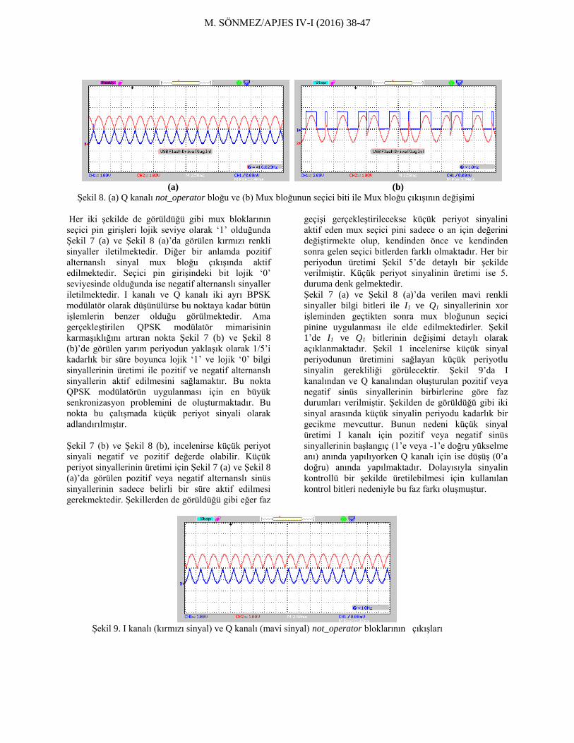
M. SÖNMEZ/APJES IV-I (2016) 38-47
(a) (a) (b)
Şekil 8. (a) Q kanalı not_operator bloğu ve (b) Mux bloğunun seçici biti ile Mux bloğu çıkışının değişimi
Her iki şekilde de görüldüğü gibi mux bloklarının
seçici pin girişleri lojik seviye olarak ‘1’ olduğunda
Şekil 7 (a) ve Şekil 8 (a)’da görülen kırmızı renkli
sinyaller iletilmektedir. Diğer bir anlamda pozitif
alternanslı sinyal mux bloğu çıkışında aktif
edilmektedir. Seçici pin girişindeki bit lojik ‘0’
seviyesinde olduğunda ise negatif alternanslı sinyaller
iletilmektedir. I kanalı ve Q kanalı iki ayrı BPSK
modülatör olarak düşünülürse bu noktaya kadar bütün
işlemlerin benzer olduğu görülmektedir. Ama
gerçekleştirilen QPSK modülatör mimarisinin
karmaşıklığını artıran nokta Şekil 7 (b) ve Şekil 8
(b)’de görülen yarım periyodun yaklaşık olarak 1/5’i
kadarlık bir süre boyunca lojik ‘1’ ve lojik ‘0’ bilgi
sinyallerinin üretimi ile pozitif ve negatif alternanslı
sinyallerin aktif edilmesini sağlamaktır. Bu nokta
QPSK modülatörün uygulanması için en büyük
senkronizasyon problemini de oluşturmaktadır. Bu
nokta bu çalışmada küçük periyot sinyali olarak
adlandırılmıştır.
Şekil 7 (b) ve Şekil 8 (b), incelenirse küçük periyot
sinyali negatif ve pozitif değerde olabilir. Küçük
periyot sinyallerinin üretimi için Şekil 7 (a) ve Şekil 8
(a)’da görülen pozitif veya negatif alternanslı sinüs
sinyallerinin sadece belirli bir süre aktif edilmesi
gerekmektedir. Şekillerden de görüldüğü gibi eğer faz
geçişi gerçekleştirilecekse küçük periyot sinyalini
aktif eden mux seçici pini sadece o an için değerini
değiştirmekte olup, kendinden önce ve kendinden
sonra gelen seçici bitlerden farklı olmaktadır. Her bir
periyodun üretimi Şekil 5’de detaylı bir şekilde
verilmiştir. Küçük periyot sinyalinin üretimi ise 5.
duruma denk gelmektedir.
Şekil 7 (a) ve Şekil 8 (a)’da verilen mavi renkli
sinyaller bilgi bitleri ile I1 ve Q1 sinyallerinin xor
işleminden geçtikten sonra mux bloğunun seçici
pinine uygulanması ile elde edilmektedirler. Şekil
1’de I1 ve Q1 bitlerinin değişimi detaylı olarak
açıklanmaktadır. Şekil 1 incelenirse küçük sinyal
periyodunun üretimini sağlayan küçük periyotlu
sinyalin gerekliliği görülecektir. Şekil 9’da I
kanalından ve Q kanalından oluşturulan pozitif veya
negatif sinüs sinyallerinin birbirlerine göre faz
durumları verilmiştir. Şekilden de görüldüğü gibi iki
sinyal arasında küçük sinyalin periyodu kadarlık bir
gecikme mevcuttur. Bunun nedeni küçük sinyal
üretimi I kanalı için pozitif veya negatif sinüs
sinyallerinin başlangıç (1’e veya -1’e doğru yükselme
anı) anında yapılıyorken Q kanalı için ise düşüş (0’a
doğru) anında yapılmaktadır. Dolayısıyla sinyalin
kontrollü bir şekilde üretilebilmesi için kullanılan
kontrol bitleri nedeniyle bu faz farkı oluşmuştur.
Şekil 9. I kanalı (kırmızı sinyal) ve Q kanalı (mavi sinyal) not_operator bloklarının çıkışları

M. SÖNMEZ/APJES IV-I (2016) 38-47
(a) (b)
Şekil 10. (a) I ve (b) Q kanalı mux bloğu çıkışı (kırmızı renkli sinyaller) ile QPSK (mavi renkli sinyal) sinyalin değişimi
Şekil 10’da ise kırmızı renkli sinyaller I ve Q
kanalında kullanılan mux bloğunun çıkışını
gösterirken kırmızı renkli sinyal I kanalında
kullanılan mux bloğunun çıkışını göstermektedir.
Şekilden görüldüğü gibi QPSK müdülasyonlu sinyal I
ve Q kanal bitlerinin durumuna göre ya I kanalındaki
sinyali ya da Q kanalındaki sinyali aktif ederek QPSK
sinyalini üretmektedirler.
(a) (b)
Şekil 11 (a)-QPSK sinyali. (b)-I kanalı biti ve Q kanalı biti sinyalleri
Şekil 11’de görüldüğü gibi veri bitlerine göre elde
edilen QPSK sinyal başarılı bir şekilde elde
edilmiştir. Şekil 11’de veri bitlerinin başlangıcı
osiloskobun soldan üçüncü karesinden başlanırsa ilk
bitler “11” olarak görülecektir. QPSK sinyal de tam
olarak soldan ikinci kare içerisinde değişim
göstermiştir ve “11” bilgi sinyalleri için başlangıç
noktası bu noktadır. Bütün durumlar (dört durum: 11,
01, 10, 00) için QPSK sinyalin oluşumu
gösterilmiştir.
Önerilen QPSK modülatör mimarisi incelenirse I
kanalı ve Q kanalı mux bloklarının çıkışları sonucu
verecek son bir mux bloğunun girişine
uygulanmaktadır. Son aşamadaki mux bloğunun
çıkışı ise bilgi sembolünü oluşturan bitlerin aynı ve
farklı olmasına göre I kanalı ve Q kanalı
sinyallerinden birisini çıkışa aktaracaktır. Dolayısıyla
Şekil 10, ve Şekil 11 (b)’den görüldüğü gibi bilgi
sembolünü oluşturan bitler farklıysa Şekil 10 (a)’da
görülen kırmızı renkli sinyal, aynıysa Şekil 10 (b)’de
görülen kırmızı renkli sinyal iletilecektir. Dolayısıyla
Şekil 11 (b)’de verilen bilgi bitleri incelenirse ilk
durumda I kanalından iletilen bitin (mavi renkli
sinyal) ‘1’, Q kanalından iletilen bitin (kırmızı renkli
sinyal) de ‘0’ olduğu görülmektedir. Dolayısıyla
bitler farklı olduğundan dolayı I kanalı sinyali son
aşamadaki mux bloğu çıkışında aktif edilerek QPSK
sinyali oluşturulur (Şekil 10 (a) ve Şekil (b)’de
görülen mavi renkli sinyaller). Bu bilgi bitlerinden bir
sonraki bitler birbiriyle aynı olduğundan dolayı
(“00”) algoritmanın son katmanındaki mux bloğu Q
kanalından iletilen sinyali aktif etmiştir.
Kaynaklar
[1] M. Nozaki, S. Yoshizawa, and Hiroshi Tanimoto,
"VLSI Design of an Interference Canceller for QPSK
OFDM-IDMA Systems", IEEE Asia Pacific
Conference on Circuits and Systems (APCCAS),
Ishigaki, Japonya, 715-718, (2014).
[2] H. M. Thien, N. Sugii, and K. Ishibashi, "A 1.36
μW 312–315MHz synchronized-OOK receiver for
wireless sensor networks using 65nm SOTB CMOS
technology", Journal of Solid-State Electronics, vol.
117, no. 1, pp. 161-169, Mar. 2016.
[3] P. Bhagawat, R. Dash, and C. Gwan,
"Architecture for reconfigurable MIMO detector and
its FPGA implementation", 15th IEEE International

M. SÖNMEZ/APJES IV-I (2016) 38-47
Conference on Electronics, Circuits and Systems,
Denver, ABD, 61-64, (2008).
[4] L., Jri, Y. Chen, and Y. Huang, "A low-power
low-cost fully-integrated 60-GHz transceiver system
with OOK modulation and on-board antenna
assembly." IEEE Journal of Solid-State Circuits, vol.
45, no. 2, pp. 264-275, Feb. 2010.
[5] D. Denis, and A. P. Chandrakasan. "An energy-
efficient OOK transceiver for wireless sensor
networks." IEEE Journal of Solid-State Circuits, vol.
42, no. 5, pp. 1003-1011, May. 2007.
[6] Z. He, W. Wu, J. Chen, Y. Li, D. Stackenas, and
H. Zirath, "An FPGA-based 5 Gbit/s D-QPSK
modem for E-band point-to-point radios", 41st
European Microwave Conference (EuMC),
Manchester, İnglitere, 690-692, (2011).
[7] S.O. Popescu, A.S.Gontean, and D.Ianchis,
"QPSK Modulator on FPGA", IEEE 9th International
Symposium on Intelligent Systems and Informatics,
Subotica, Sırbistan, 359-364, (2011).
[8] W. Song, and Q. Yao, "Design and Implement of
QPSK Modem Based on FPGA", IEEE International
Conference on Computer Science and Information
Technology, Chengdu, Çin, 599-601, (2010).
[9] T. Kazaz, M. Kulin, and M. Hadzialic, "Design
and Implementation of SDR Based QPSK Modulator
on FPGA", MIPRO 2013, Opatija, Hırvatistan, 513-
518, (2013).
[10] X. Xiquan, "Implementation of PSK Digital
Demodulator with Variable Rate Based on FPGA",
Open Automation and Control Systems Journal, vol.
7, no. 2, pp.1280-1286, Sep. 2015.
[11] Y. Linn, "A Self-Normalizing Symbol
Synchronization Lock Detector for QPSK and
BPSK", IEEE Transactions on Wireless
Communıcations, vol. 5, no. 2, pp. 347-353, Feb.
2006.
[12] J. Bao, C.Y. Lu, P. D. Graca, S. Zeng, and T.
Poon, "A New Timing Recovery Method For DTV
Receivers", IEEE Transactions on Consumer
Electronics, vol. 44, no. 4, pp. 1243-1249, Nov. 1998.
[13] A. Tolmachev, I. Tselniker, M. Meltsin, I.
Sigron, D. Dahan, A. Shalom, and M. Nazarathy,
"Multiplier-Free Phase Recovery With Polar-domain
Multisymbol-Delay-Detector", Journal of Lightwave
Technology, vol. 31, no. 23, pp. 3638-3650, Dec.
2013.
[14] P. P. Schönwälder, J. B. Dalmau, F. X. Geniz, F.
A. López, and R. G. Mas "A Superregenerative QPSK
Receiver", IEEE Transactions on Circuıts and
Systems—I: Regular Papers, Vol. 61, No. 1, pp. 258-
265, Jan. 2014
[15] N. K. Venkatachalam, L. Gopalakrishnan, M.
Sellathurai, "Low complexity and area efficient
reconfigurable multimode interleaver address
generator for multistandard radios", IET Computers
& Digital Techniques, vol. 10, no. 2, pp. 59-68, Mar.
2016.
[16] S. Ertürk, "Sayısal Haberleşme", Birsen
Yayınevi, İstanbul, 2005.