Embed Size (px)
Citation preview

Volume 6, No. 4, 2003ISSN 1077-291X
The Journal of Public Transportation is published quarterly by
National Center for Transit ResearchCenter for Urban Transportation Research
University of South Florida • College of Engineering4202 East Fowler Avenue, CUT100
Tampa, Florida 33620-5375Phone: 813•974•3120
Fax: 813•974•5168Email: [email protected]
Website: www.nctr.usf.edu/journal
© 2003 Center for Urban Transportation Research
PublicTransportation
JOURNAL OF

Gary L. Brosch, EditorLaurel A. Land, AICP, Managing Editor
EDITORIAL BOARD
Robert B. Cervero, Ph.D. William W. MillarUniversity of California, Berkeley American Public Transportation Association
Chester E. Colby Steven E. Polzin, Ph.D., P.E.E & J Consulting University of South Florida
Gordon Fielding, Ph.D. Sandra Rosenbloom, Ph.D.University of California, Irvine University of Arizona
David J. Forkenbrock, Ph.D. Lawrence SchulmanUniversity of Iowa LS Associates
Jose A. G\mez-Ib<ñez, Ph.D. George Smerk, D.B.A.Harvard University Indiana University
Naomi W. LedJ, Ph.D.Texas Transportation Institute
The contents of this document reflect the views of the authors, who are responsible for the facts andthe accuracy of the information presented herein. This document is disseminated under thesponsorship of the U.S. Department of Transportation, University Research Institute Program, in theinterest of information exchange. The U.S. Government assumes no liability for the contents or usethereof.

SUBSCRIPTIONS
Complimentary subscriptions can be obtained by contacting:
Laurel A. Land, Managing EditorCenter for Urban Transportation Research (CUTR) • University of South Florida4202 East Fowler Avenue, CUT100 • Tampa, FL 33620-5375Phone: 813•974•1446Fax: 813•974•5168Email: [email protected]: www.nctr.usf.edu/journal.htm
SUBMISSION OF MANUSCRIPTS
The Journal of Public Transportation is a quarterly, international journal containing originalresearch and case studies associated with various forms of public transportation and relatedtransportation and policy issues. Topics are approached from a variety of academic disci-plines, including economics, engineering, planning, and others, and include policy, method-ological, technological, and financial aspects. Emphasis is placed on the identification ofinnovative solutions to transportation problems.
All articles should be approximately 4,000 words in length (18-20 double-spaced pages).Manuscripts not submitted according to the journal’s style will be returned. Submission ofthe manuscript implies commitment to publish in the journal. Papers previously publishedor under review by other journals are unacceptable. All articles are subject to peer review.Factors considered in review include validity and significance of information, substantivecontribution to the field of public transportation, and clarity and quality of presentation.Copyright is retained by the publisher, and, upon acceptance, contributions will be subjectto editorial amendment. Authors will be provided with proofs for approval prior to publi-cation.
All manuscripts should be submitted electronically, double-spaced in Word file format.Manuscripts should consist of type and equations only. Footnotes should be grouped at theend of the text. Charts, tables, and graphs should be in Excel format. Each drawing, diagram,picture, and/or photograph must be in black and white and submitted separately in itsoriginal format, having a minimum 300 dpi. Each chart and table must have a title, and eachfigure must have a caption.
All manuscripts should include sections in the following order, as specified:
Cover Page – title (12 words or less), and short biographical sketch of all authorsFirst Page of manuscript – title and abstract (up to 150 words)Main Body – organized under section headingsReferences – Chicago Manual of Style, author-date format
Be sure to include the author’s complete contact information, including email address,mailing address, telephone, and fax number. Submit manuscripts to the Managing Editor, asindicated above.

Volume 6, No. 4, 2003ISSN 1077-291X
CONTENTS
The Importance Customers Place on Specific Service Elements ofBus Rapid TransitMichael R. Baltes ......................................................................................................................................... 1
Bus Transit and Land Use:Illuminating the InteractionAndy Johnson .............................................................................................................................................. 21
Evaluating the Urban Commute Experience:A Time Perception ApproachYuen-wah Li .................................................................................................................................................. 41
A Review of Approaches for Assessing MultimodalQuality of ServiceRhonda G. Phillips, Martin Guttenplan ........................................................................................ 67
Externalities by Automobiles and Fare-Free Transit in Germany—A Paradigm Shift?Karl Storchmann ...................................................................................................................................... 87
Our troubled planet can no longer afford the luxury of pursuitsconfined to an ivory tower. Scholarship has to prove its worth,
not on its own terms, but by service to the nation and the world.—Oscar Handlin
iii

Service Elements of Bus Rapid Transit
1
The Importance Customers Placeon Specific Service Elements of
Bus Rapid TransitMichael R. Baltes
National Bus Rapid Transit Institute
AbstractAbstractAbstractAbstractAbstract
Bus Rapid Transit (BRT) is a rapidly growing national trend in the provision of publictransportation. At present, with more than 150 New Start Rail Projects currently inthe FTA pipeline, a wide range of alternatives is necessary to fulfill the demand forcost-effective rapid public transportation. As a lower cost, high-capacity mode ofpublic transportation, BRT can serve as an option to help address the growing trafficcongestion and mobility problems in both urban and nonurban areas. Carefuldocumentation and analyses of BRT systems and the unique features of these projectswill help determine the most effective features offered by the BRT systems such themost successful service characteristics, level of transit demand, region size, and otheramenities. This article presents a statistical analysis of the data from two on-boardcustomer surveys conducted in 2001 of the BRT systems in Miami and Orlando,Florida. Using data from the two on-board surveys, the simplest method for measur-ing the importance that customers place on specific BRT service characteristics is tocalculate mean scores for each characteristic using some type of numeric scale (e.g.,a scale of 1 through 5, with 5 being the highest). While there are no real discernabledrawbacks to this simple method, an alternate technique to measure the impor-tance of each service attribute is to derive the importance of each attribute usingSTEPWISE regression. This statistical method estimates the importance of each

Journal of Public Transportation, Vol. 6, No. 4, 2003
2
attribute to overall customer satisfaction. The results indicate that customers placea high value on the BRT service characteristics frequency of service, comfort, traveltime, and reliability of service.
IntroductionOne of the main goals of the Federal Transit Administration’s (FTA) Bus RapidTransit (BRT) Demonstration Program is to determine the effects of 10 nation-wide BRT demonstration projects through a scientific evaluation process. TheFTA designated the South Miami-Dade Busway, Busway for short, as one of its 10BRT demonstration sites. While not one of FTA’s 10 designated BRT demonstra-tion projects, the Lynx LYMMO in Orlando was chosen by the FTA for evaluationdue to its Intelligent Transportation Systems (ITS) and as a model for the imple-mentation of similar BRT systems. According to the FTA, careful documentationand analyses of the BRT demonstration projects and the unique features of theseprojects will help determine the most effective features (i.e., type of service offered,most successful service characteristics, level of transit demand, region size, andother amenities). It is anticipated that the BRT demonstration projects will serveas learning tools and as models for other locales throughout the country, andpossibly the world. For these demonstrations to have maximum effectiveness intheir respective operational capacities, a consistent and carefully structured ap-proach to project evaluation is necessary.
The following, taken verbatim from Evaluation Guidelines for Bus Rapid TransitDemonstration Projects (Schwenk 2001), are the four evaluation guidelines for the10 BRT demonstration projects:
1. Determine the benefits, costs, and other impacts of individual BRT fea-tures, including ITS/APTS applications, and of the system as a whole.
2. Characterize successful and unsuccessful aspects of the demonstration.
3. Evaluate the demonstration’s achievement of FTA and agency goals.
4. Assess the applicability of the demonstration results to other sites.
In addition, the FTA plans to examine specific impacts of the BRT demonstrationprojects. These impacts include: degree that bus speeds and schedule adherenceimprove; degree that ridership increases (due to improved bus speeds, scheduleadherence, and convenience); effect of BRT on other traffic; effect of each of theBRT components on bus speed and other traffic; benefits of ITS/APTS applica-tions to the demonstration project; and effect of BRT on land use and develop-

Service Elements of Bus Rapid Transit
3
ment. To meet these objectives, it is necessary to collect a variety of data on severalaspects of the BRT demonstration project, including measurable impacts to BRTcustomers via the on-board survey process.
In keeping with the FTA’s evaluation guidelines, the National Bus Rapid TransitInstitute at the Center for Urban Transportation Research (CUTR), working jointlywith Miami-Dade Transit (MDT) and Lynx, conducted on-board surveys of SouthMiami-Dade Busway customers in March 2001 and Lynx LYMMO customers inDecember 2001. The South Miami-Dade Busway and Lynx LYMMO are examplesof different applications of BRT systems that are specifically designed to offer fastertravel choices to customers compared to standard local bus service and possibly,even the private automobile. Evaluation of the various components of the Buswayand LYMMO are crucial parts of the demonstration project. The two on-boardsurveys serve as the first phase of the independent review of the Busway andLYMMO BRT systems. The second phase will include analyses of the more detailedcomponents of each BRT system, including engineering and construction, tech-nical documentation, ITS, and system performance.
The on-board surveys were conducted to assess customer perceptions, behavior,and to develop customer profiles. The survey instruments asked customers toevaluate the various BRT elements of service as well as overall satisfaction, with theultimate purpose of measuring the impacts of the systems on customer percep-tions. Other questions focused on customer behavior, including trip origins anddestinations and frequency of use.
ObjectiveThis article presents a statistical analysis of the data from two on-board customersurveys of the BRT systems in Miami and Orlando, Florida. Using data from thetwo on-board surveys, the simplest method for measuring the importance thatcustomers place on specific BRT service characteristics is to calculate mean scoresfor each characteristic using some type of numeric scale (e.g., a scale of 1 through5, with 5 being the highest). While there are no real discernable drawbacks to thissimple averaging method, an alternate technique to measure the importance ofeach service attribute is to derive the importance of each attribute to overall satis-faction using more advanced statistical procedures such as STEPWISE regression.This statistical method estimates the importance of each service attribute to over-all customer satisfaction. While there may be a degree of intercorrelation betweeneach of the service attributes, this method can be used to measure the relative

Journal of Public Transportation, Vol. 6, No. 4, 2003
4
importance of each attribute when determining what elements or combinationof elements best comprise overall customer satisfaction with these two BRT sys-tems.
South Miami-Dade and Orlando LYMMO BRT SystemsSouth Miami-Dade BuswayThe South Miami-Dade Busway, or Busway for short, is an 8-mile, two-lane bus-only roadway constructed in a former rail right-of-way (the former Florida EastCoast Railroad corridor) adjacent to US 1, a major north-south arterial in south-ern Miami-Dade County. Miami-Dade Transit (MDT) opened the first phase ofthe Busway on February 3, 1997. The Busway was designed for exclusive use bytransit buses and emergency and security vehicles. The purpose of the Buswayservice is to address the need for faster travel choices for MDT customers. Much ofthe Busway BRT service uses 20-seat minibuses to keep costs to a minimum.
Currently, there are 18 intersections and 15 stations in each direction (30 totalstations), as shown in Figure 1. The Busway corridor over much of its length iswithin 100 feet of the west side of US 1, one of the most heavily traveled corridorsin Miami-Dade County. There are several types of service in the Busway corridor:
Local—Only operates on the exclusive Busway and makes every stop at alltimes (referred to as the Busway Local).
Limited Stop—Operates along the length of the Busway and beyond, skipsstops nearest the Metrorail station during peak periods (Busway MAX orMetro Area Express).
Feeder—Collects passengers in neighborhoods and then enters the Busway ata middle point (service is known as either the Coral Reef MAX or Saga BayMAX).
Crosstown—Preexisting routes in the corridor that now take advantage of theBusway when possible. These routes enter and exit the Busway at middlepoints. These routes are designed to provide access to many destinationsin the region, not just to the center city (Routes 1, 52, and 65).
Intersecting—Routes in the corridor that intersect with Busway routes, some-times stopping at Busway stations.

Service Elements of Bus Rapid Transit
5
Figure 1. Map of South Miami-Dade Busway

Journal of Public Transportation, Vol. 6, No. 4, 2003
6
The Busway stations are located at roughly half-mile intervals, more than twice thecustomary stop spacing for conventional MDT local bus service. For example,when Route 1 operated on US 1, it had 19 designated stops southbound and 23northbound (on the portion of the route using US 1). When it was moved to theBusway, only 10 Busway stations served the same distance. Most stations are onthe far side of intersections. In two locations there are mid-block stops to servemajor generators. All stations have large shelters designed to protect customersfrom the weather. Stations platforms are in three lengths: 40 feet, 60 feet, and 80feet. Busway vehicles operate parallel in a bidirectional manner with vehicular traf-fic operating separate from Busway vehicles.
According to MDT, bus ridership on the U.S. 1 corridor in South Miami-DadeCounty increased greatly with the implementation of the Busway service. As aresult of Busway service, ridership in the corridor increased by 49 percent onweekdays, 69 percent on Sundays, and 130 percent on Saturdays since May 1998.MDT staff indicated that the major reasons for the increases in ridership were theincrease in service provided, in terms of new areas served, more frequent service,and a greater span of service. Except for Saturdays, revenue miles increased evenfaster than boardings and operating costs increased at only half the rate of theincrease in vehicle revenue miles—due to the use of 20-seat minibuses, which costthe MDTA $31 to $35 per hour to operate, significantly less than the $51 to $53per hour it costs to operate full-size buses. The difference in cost is due to fuel andmaintenance costs and to the lower wages paid to minibus operators.
Orlando LYMMOThe LYMMO BRT system is very different in application from the Busway oper-ated by MDT. It operates on a 3-mile continuous loop through Downtown Or-lando using a combination of the various types of dedicated running ways includ-ing median and same-side travel way configurations. The exclusive running waysare paved with distinctive gray-colored pavers to delineate them from generaltraffic lanes. They are separated from general traffic lanes either with a raised me-dian or a double row of raised reflective ceramic pavement markers embedded inthe asphalt.
Because the LYMMO operates in places and directions contrary to other traffic, allbus movements at intersections are controlled by special bus signals. To preventmotorist confusion, these signal heads use lines instead of the standard red, yel-low, and green lights. When a LYMMO bus approaches an intersection, an em-

Service Elements of Bus Rapid Transit
7
Figure 2. Map of the LYMMO System

Journal of Public Transportation, Vol. 6, No. 4, 2003
8
bedded loop detector in the dedicated running way triggers the intersection toallow the bus to proceed either in its own signal phase or at the same time as othertraffic is released when no conflicting traffic movements are permitted.
The LYMMO uses 10 low-floor vehicles fueled by environmentally friendly com-pressed natural gas. The vehicles use high-quality, modern interiors that incorpo-rate the Transit TV Network, an ITS system. The Transit TV Network provides real-time information such as Downtown events, weather, and fun and trivia to cus-tomers. In addition, public art exteriors are used on the vehicles to enhance thecustomer’s experience with the LYMMO. The LYMMO system has 11 lighted andcomputerized stations and 9 additional stops, as shown in Figure 2.
LYMMO vehicles operate approximately every 5 minutes during office hours; afteroffice hours, vehicles operate approximately every 10 minutes. Since the inceptionof service, the LYMMO has been free to ride during all hours of operation. Opera-tion and maintenance of the LYMMO is 100 percent funded by revenue generatedby the City of Orlando’s Parking and Enterprise Fund. The LYMMO operates from6 A.M. to 10 P.M., Monday through Thursday, 6 A.M. to midnight on Friday, 10A.M. to midnight on Saturday, and 10 A.M. to 10 P.M. on Sunday. LYMMO’starget market is customers who drive to Downtown Orlando and then useLYMMO to get to other Downtown locations, such as the courthouse, restau-rants, shopping, and other land uses.
For comparison, Table 1 shows the key components of the both the Busway andLYMMO BRT systems.
Survey Methodology and Statistical ProceduresThe Busway survey instrument was printed in English on one side and Spanish onthe other due to the bilingual nature of Miami. It contained 18 questions andprovided space for additional written comments by customers. The LYMMOsurvey instrument was printed in English only and contained a total 13 questions.NBRTI/CUTR and MDT and Lynx staff developed the survey instruments jointly.
The on-board surveys specifically targeted customers riding only those routesthat operate along the Busway for either all or a portion of their trips and for all ora portion of their trips in Downtown Orlando on the LYMMO. At least half of alltrips on a particular Busway route were selected for surveying. For example, ifthere were eight trips on a route, four were to be surveyed. If there were nine trips,five were surveyed. The trips selected for survey distribution spanned the service

Service Elements of Bus Rapid Transit
9
hours (i.e., morning peak, midday off-peak, afternoon peak, and evening). For theLYMMO, surveying began at the start of service and concluded at about 7 P.M.Given that the typical weekday LYMMO schedule consists of about 186 21-minuteround trips (circulations) and the last trip begins at 10 P.M., this translates intojust over 90 percent of all weekday trips being included in the sample.
Surveyors were instructed to offer a survey form to each customer upon boardinga bus. Every time a customer boarded a Busway or LYMMO vehicle to make asubsequent trip (regardless of the whether the trip was their second, third, fourth,and so on), they were asked to complete another survey. Surveyors were instructedto do the best they could to encourage participation in the survey. If a surveycould not be handed directly to a customer, surveyors were instructed to “drop”a survey in each vehicle seat. All surveys were collected on-board buses. No mail-back provision was provided for returning the completed surveys.
Key BRT AttributesBusway LYMMO
Yes No Yes No
Simple route structure ✔ ✔
Frequent service ✔ ✔
Headway-based schedules ✔ ✔
Less frequent stops ✔ ✔
Level boarding and alighting ✔ ✔
Color-coded buses ✔ ✔
Color-coded stations/stops ✔ ✔
Bus signal priority ✔ ✔
Exclusive lanes ✔ ✔
Modern vehicle interiors ✔ ✔
Higher-capacity buses ✔ ✔
Multiple door boarding and alighting ✔ ✔
Off-vehicle fare payment ✔ ✔
Feeder network ✔ ✔
ITS/APTS on vehicles ✔ ✔
ITS/APTS at stations ✔ ✔
Coordinated land-use planning ✔ ✔
Table 1. Key Bus Rapid Transit Components

Journal of Public Transportation, Vol. 6, No. 4, 2003
1 0
Once collected, survey data were entered into an Excel spreadsheet for archivingand later analyses. CUTR staff performed the review and data analyses using SPSS(Statistical Product and Service Solutions) software.
Prior to the analyses, survey responses were weighted based on the total weekdayridership and completed surveys for each route to more accurately reflect Buswayand LYMMO ridership as a whole. Weighting factors were derived to ensure properrepresentation of Busway and LYMMO customers. Specifically, weights were cal-culated by dividing the total weekday ridership (obtained from MDT and Lynxstaff) for the survey period by the number of surveys returned. The resultingweight factors were applied to each completed survey’s data for statistical analysis.The survey methodologies involved the survey of willing customers. The method-ologies correspond most closely with ridership data that are reported as unlinkedtrips. Table 2 indicates Busway ridership figures for March 19–23, 2001 and Table3 shows ridership for the LYMMO for December 20, 2001. The data in Table 2 arerepresentative of the five-day (Monday through Friday) total weekday ridershipand the data in Table 3 represent monthly LYMMO patronage. Daily ridershipfigures were not available for either of the two BRT systems.
Table 2. Weekday Busway Ridership (March 19–23, 2001)
Entire Route Weekday Ridership* Percent of Ridership on TripsSurveyed
1 8,182 17.4
31/231 (Busway Local) 8,820 18.8
38 (Busway MAX) 17,368 37.0
52 6,619 14.1
252 (Coral Reef MAX) 4,491 9.6
287 (Saga Bay MAX) 1,491 3.2
Total Busway routes ridership 46,971 100
* Total weekday ridership for the entire route length.

Service Elements of Bus Rapid Transit
1 1
The response rates for the on-board surveys of Busway and LYMMO customersranged from a low of 6.45 percent to 23.7 percent. Although somewhat low, theseresponse rates are fairly usual for surveys of this type where prior experience hasshown them to be in the 10 to 20 percent response range. It should be noted thatthe following results are based on a sample of system users and not a 100 percentcensus. There is the chance of some customers not choosing these two BRT sys-tems because they felt that additional factors not discussed in the results weremore important to their selection of mode choice. In addition, survey instru-ments were not originally designed to ask customers of these two BRT systemsabout their satisfaction with the Busway and LYMMO compared to other alterna-tives such as standard local bus. For example, the Busway survey could have in-cluded a question asking respondents to indicate their satisfaction with the traveltime on Busway buses versus the travel time on standard local Miami-Dade Transitbus service. Everyone has a different approach to determining satisfaction withthe various components that comprise a particular mode including travel timeand frequency of service, for example. It is only when customers are asked todirectly compare the various BRT components to those of other modes thatcomparable results can be obtained. Nevertheless, the results presented in thisarticle show the measurement of actual customer satisfaction with the two BRTsystems. Currently, there are many BRT systems in the planning and design phasesas well as in operation that will benefit from the results presented in this article.
Table 3. Monthly LYMMO Ridership (December 2001)
Week (Saturday through Friday) Ridership Proportion of Ridership on TripsSurveyed
December 1-7 20,618 27.8
December 8-14 20,592 27.8
December 15-21 19,992 27.0
December 22-28 10,304 13.9
December 29-31 2,541 3.4
Total ridership 74,047 100

Journal of Public Transportation, Vol. 6, No. 4, 2003
1 2
Measuring the Importance of BRT ElementsMean ScoresQuestions 17 (Busway) and 13 (LYMMO) on the survey instruments were multi-part questions that asked customers to rate their perception of different aspectsof Busway and LYMMO BRT services, using five-point scales (1 = “very dissatisfied”and 5 = “very satisfied”). Each survey included a question that asked about overallcustomer satisfaction with the BRT services offered by both systems.
These two questions offered customers an opportunity to rate their individuallevels of satisfaction with various service characteristics. Using the five-point ratingsystem’s numerical scoring values, an average score was calculated for each servicecharacteristic. The resulting mean scores give a good indication of overall cus-tomer satisfaction with each of the service aspects. Since a score of 5 indicates a“very satisfied” rating, the closer to 5 that a characteristic’s mean score is, the higherthe degree of customer satisfaction is with that particular characteristic.
Table 4 presents all of the weighted average customer satisfaction ratings for theservice characteristics included in the surveys. The responses indicate a very highlevel of satisfaction with the services offered by the Busway and LYMMO; all meanscores fell between “neutral” and “very satisfied,” including the aspects travel timeand reliability. An analysis of the very high customer mean scores and importanceof the service attributes inquired about clearly shows that users regard the Buswayand LYMMO BRT systems as premium services.
STEPWISE RegressionThe simplest way to measure the importance that customers of public transitplace on specific service characteristics is to calculate mean scores for each charac-teristic on some type of numeric scale (e.g., a scale of 1 through 5). While there areno real discernable drawbacks to this simple method, an alternate and more ad-vanced technique to measure the importance of each service attribute is to deriveimportance by examining the relationship of each attribute to overall customersatisfaction. This methodology uses STEPWISE regression analysis to estimate theimportance of each service attribute. While there is a degree of intercorrelationbetween each of the service attributes, this method can be used to measure therelative importance of each attribute when determining what elements or combi-nation of elements comprise overall customer satisfaction of these two BRT sys-tems. By using STEWISE regression, the r-squared values can be used as surrogatesfor customer satisfaction.

Service Elements of Bus Rapid Transit
1 3
The STEPWISE regression analysis enters independent factors (each BRT servicecharacteristic) one at a time, backwards and forwards, to determine which onehas the highest correlation with the dependent factor (in this case, overall cus-tomer satisfaction). Additional independent factors are entered into the regres-sion equation only when they make a significant contribution to the predictivepower of the equation. During the process, if any of the independent factors fallsbelow the specified criterion, it is removed automatically from the equation build-ing process. In this case, the criterion for entering the regression equation was p <0.05, and the criterion for removal from the regression equation was p > 0.10. TheSTEPWISE regression analysis resulted in all four of the service characteristics enter-ing the regression equation, accounting for 69.3 percent of the customers’ overallsatisfaction with the LYMMO service. For the Busway, the STEPWISE regressionanalysis resulted in all eight of the service characteristics entering the regressionequation, accounting for 67.3 percent of the customers’ overall satisfaction with
Table 4. Means Satisfaction Scores for Busway and LYMMO
CharacteristicsMean Score
Busway LYMMO
Safety on bus 3.81 4.41
Availability of seats on the bus/comfort 3.60 4.41
Dependability of buses (headway adherence) 3.18 4.47
Travel time on buses 3.63 4.48
Cost of riding buses 3.76 Not asked
Availability of information/maps 3.69 Not asked
Convenience of routes 3.69 Not asked
Satisfaction with recent changes to Busway 3.68 Not asked(traffic signals)
Safety at Busway stops 3.65 Not asked
Hours of Busway service 3.50 Not asked
Frequency of Busway service 3.25 Not asked

Journal of Public Transportation, Vol. 6, No. 4, 2003
1 4
Table 6. Results from Busway Customer Satisfaction STEPWISE Analysis
Table 5. Results from LYMMO Customer Satisfaction STEPWISE Analysis
ModelModel Independent R R-Square Adjusted Std. Error ofDepend.
Variables R-Square the EstimateVariable
Comfort 0.750 0.563 0.563 0.473
Comfort + Travel Time 0.810 0.656 0.656 0.419
Comfort + Travel Time + 0.830 0.689 0.689 0.399Reliability of Service
Comfort + Travel Time + 0.832 0.692 0.693 0.396Reliability of Service + Safety
overallcustomer
satisfaction
ModelModel/Service R R-Square Adjusted Std. Error ofDepend.Characteristics R-Square the EstimateVariable
Frequency of Service 0.694 0.481 0.480 0.734
Frequency of Service + 0.771 0.594 0.593 0.649Convenience
Frequency of Service + 0.792 0.628 0.627 0.622Travel Time + Seat Availability
Frequency of Service + 0.805 0.649 0.647 0.605Travel Time + Seat Availability+ Convenience
Frequency of Service + 0.814 0.662 0.660 0.594Travel Time + Seat Availability+ Convenience + Hrs of Service
Frequency of Service + 0.818 0.669 0.667 0.588Travel Time + Seat Availability+ Convenience + Hrs of Service+ Safety on Bus
Frequency of Service + 0.821 0.674 0.671 0.584Travel Time + Seat Availability+ Convenience + Hrs of Service+ Safety on Bus + Dependability
Frequency of Service + 0.823 0.677 0.673 0.582Travel Time + Seat Availability+ Convenience + Hrs of Service+ Safety on Bus + Dependability
overallcustomer
satisfaction

Service Elements of Bus Rapid Transit
1 5
Busway service. Or, put another way, these service characteristics aided in under-standing between almost 64 and 70 percent of overall customer satisfaction withthe Busway and LYMMO services, as shown in Tables 5 and 6.
Busway
For the Busway, the first three-service characteristic to enter the regressionequation were “frequency of service,” “travel time,” and “seat availability”(comfort). These three independent variables accounted for 62.7 percent ofthe equations overall predictive power, or overall customer satisfaction withthe Busway. This finding is not surprising given the results for the simplemean scores for these service aspects where Busway customers rated eachhighly given the more “rapid” (real or perceived) nature of Busway servicecompared to MDT local service. Each of these service aspects (independentvariables) is an important element of BRT service. The remaining serviceaspects to enter into the Busway STEPWISE regression model were, in orderof entry, “convenience of routes,” “hours of service,” “safety on Buswayvehicles,” dependability (on-time performance), and the availability of routeinformation. These remaining five variables added only 4.6 percent to themodels overall predictive power. All of the service characteristics are signifi-cant at the p < 0.05 level.
However, one important Busway service characteristic, “cost of riding thebus,” did not enter into the regression equation as originally hypothesized.This result is counterintuitive to what is assumed about the factors thatcustomers weigh in their decision to use local bus service. However, with apremium service such as that offered by a BRT system, it appears that cost isless of a concern than the overall quality of the BRT service and traveltimesavings offered to customers. By its omission in the regression model,the data seem to indicate that if high quality premium service is offered,persons are willing to pay a little extra for the additional benefits of such asystem.
LYMMO
The first service characteristic to enter the regression equation was “comfortof the LYMMO vehicles,” accounting for 56.3 percent of the equationsoverall predictive power. This result is not surprising given that customersindicated that they liked the low-floor vehicles and modern vehicle interiorsthe most, each of these an important “comfort” element and aspect of BRTservice. The second service characteristic to enter the regression equationwas “travel time on LYMMO vehicles.” The entry of “travel time” into the
Journal of Public Transportation, Vol. 6, No. 4, 2003
1 6
regression equation increased its overall predictive power to 65.6 percent, asignificant increase in predictive power. Again, this result is not too surpris-ing given that LYMMO customers indicated that they elected to use theLYMMO service because it is faster than walking to their destination. Thisfinding is consistent with the “rapid” or “perceived rapid” nature of BRTservices such as the LYMMO. The third variable to enter the regressionequation was “reliability of LYMMO service.” Interestingly, this servicecharacteristic only marginally increased the overall predictive power of theregression model. This result is somewhat hard to explain, given thatcustomers of public transit systems typically put a high premium on vehiclereliability that includes both on-time performance and vehicle breakdowns.The same holds true for the final service characteristic, “safety on vehicles,”that entered into the regression equation. This service characteristicincreased the predictive or explanatory power of the overall regressionequation by only 0.004 percent. All of the service characteristics are signifi-cant at the p < 0.05 level.
Discussion and ConclusionsBased on the results of the STEPWISE regression analysis, it appears that an argu-ment could be made for a narrow and comprehensive set of traits as the basis fordefining and providing different applications of BRT service. Based on the idea ofproviding a premium service that is more comfortable, frequent, rapid, and reli-able than “typical” local bus service or other modes, BRT could be treated as anattempt to inject new energy and life into stagnant local transit bus services. Build-ing on the results from this analysis, the unique services aspects of BRT that can beadded to improve other bus services is good for all concerned.
Much discussion of late in the transit industry has been made about how to makeBRT distinct and different from standard local service within an individual transitsystem. The answer may be found not in the type of vehicles that are provided toriders, but found mainly in the quality of BRT service that is ultimately offered.One only has to look at the success (increased ridership, decreased travel times) ofthe different BRT applications in Los Angeles; Pittsburgh; Ottawa, Canada; Brisbane,Australia; and Curitiba, Brazil to see the virtue of this statement. All of these BRTsystems provide extremely frequent, reliable, easy to use, comfortable, safe, andfast (rapid) service (even in mixed traffic) essentially using conventional-lookingbuses. The results from the STEPWISE regression analysis seem to suggest thatthese systems are providing the right mix of service aspects to foster sustainedpatronage and growth. Perhaps what the customer really wants is to get from

Service Elements of Bus Rapid Transit
1 7
home to work and back again in the shortest time with the greatest overall level ofcomfort and personal safety (and to a degree, the cost of riding may not be anoverriding factor). The results from this article suggest that future customers willrely more on the quality of the BRT service that’s offered than any other aspect.Again, the success in terms of ridership gains and public acceptance of the Buswayand LYMMO provide ample evidence to support this suggestion.
Based on MDT analysis, the Busway seems to have provided little or no traveltimesavings for Busway vehicles compared to existing local service—yet, ridershipin the corridor increased by 49 percent on weekdays, 69 percent on Sundays, and130 percent on Saturdays since May 1998. This increase is mostly explained by the72 percent increase in weekly revenue miles. This suggests that the MDT manage-ment did a good job of listening to customers when deploying and implementingBusway service. The combination of Busway service characteristics including highfrequency, both in the peak and off-peak, travel time (real or perceived), and seatavailability (comfort) are clearly central factors leading to this success.
Lynx reports that despite exclusive running ways and signal preemption, averageroundtrip speeds are not as great as expected and are one-third slower on theLYMMO than its downtown predecessor the FreeBee. The reasons for this arehard to discern. One possible explanation is that LYMMO buses stop at eachstation, whether customers are waiting or not. Another possibility is that in-creased ridership has resulted in additional station dwell time during the boardingand alighting process—despite the use of low-floor vehicles and no fare collec-tion. Despite the slow average system speed, LYMMO ridership has increased dra-matically since system implementation—the real measure of success. Additionalpossible sources for increased ridership other than increased service hours is thecreation of an overall pleasant and safe riding experience, an aggressive marketingcampaign, comfort of the LYMMO vehicles, travel time (whether real or perceived)of LYMMO vehicles, reliability of LYMMO service, and safety on LYMMO vehiclesand at stations.
Every customer of public transit has a different approach to determining theirsatisfaction with the various components that comprise a particular mode in-cluding travel time and frequency of service, for example, and their decision to usethat mode at any given time. There is a chance that factors not present in the twoBRT systems analyzed in this article could have caused customers not to choicethe BRT mode for their trip making. For example, the Transit Cooperative Re-search Program (TCRP) Report 47 (1999) offers many different potential mea-

Journal of Public Transportation, Vol. 6, No. 4, 2003
1 8
sures of transit service quality including overcrowding, bilingual signage andsystem information, quietness of vehicles, fairness of fare structure, announce-ments of delays, cost of making transfers, absence of offensive odors, ease of pay-ing fare, number of transfer points outside of the downtown core, courteoussystem staff, physical condition of stations, station access, posted minutes to nextbus, and so on in addition to the factors presented in this article. The surveyinstruments used to gather information for this article were not originally de-signed to ask customers about every possible service characteristic related to theBusway and LYMMO. Nevertheless, the results presented here show the measure-ment of actual customer satisfaction with important service characteristics of thetwo BRT systems and those elements that are important to all BRT systems. Atpresent, there are many BRT systems in the planning and design phases as well asin operation that will benefit from the results presented in this article even using alimited number of service quality measures to determine overall customer satisfac-tion.
Although the R2 –values are fairly high even with the small number of indepen-dent factors (4 for the LYMMO and 10 for the Busway), it is important to notethat about 33 percent of with the Busway and 31 percent with the LYMMOservice related to overall customer satisfaction remains unexplained. As part of theBRT evaluation processes, a number of focus groups will be conducted that couldaid in uncovering the remaining factors related to overall customer satisfaction.Certainly, the four service characteristics included in the regression equation makeit clear that they are important factors to customers of this BRT system. However,the unexplained variance also makes it clear that a full understanding behind thedynamics of customer satisfaction may require the inclusion of additional inde-pendent variables in futures regression analyses as noted in the preceding para-graph. These service characteristics would certainly include those present in otherBRT systems or perhaps psychological factors related to customer satisfaction.
While BRT is the talk of the U.S. public transit industry (and even the global transitindustry), there is still a long way to go to make this a successful and publiclyaccepted mode of public transportation as in other places including Canada,South America, Australia, and Europe. There is a continued need for marketing,vehicle development, data collection, project evaluation, an updated AlternativesAnalysis process to include BRT, revised New Starts eligibility criteria, research, andadditional technology transfer. The author supports the statements made by theFTA that no single mode of public transportation is right for all situations. How-

Service Elements of Bus Rapid Transit
1 9
ever, given the incontestable merits of BRT, it should receive serious considerationas an important alternative in the planning toolkit.
References
Schwenk, J.C. 2002. Evaluation guidelines for Bus Rapid Transit DemonstrationProjects. DOT-VNTSC-FTA-02-02, DOT-MA-26-7033-02. February.
Transit Cooperative Research Program. 1999. TCRP Report 47—A handbook formeasuring customer satisfaction and service quality. Washington D.C.: Trans-portation Research Board, National Research Council.
Los Angeles County Metropolitan Transportation Authority. Metro Rapid Evalua-tion Before and After Survey Results. Unpublished paper, date unknown.
Henke, Cliff. A Practical Approach to Bus Rapid Transit. Unpublished paper. NorthAmerican Bus Industries, Woodland Hills, CA, 2002.
U.S. General Accounting Office. Bus Rapid Transit Shows Promise. September 2001.
Levinson, Herbert S. et al., Bus Rapid Transit Synthesis of Case Studies. Presented atthe Annual Meeting of the 2003 Transportation Research Board and sched-uled for publication in an upcoming Transportation Research Record.
About the Author
MICHAEL R. BALTES ([email protected]) is a senior research associate at the Na-tional Bus Rapid Transit Institute (NBRTI) located at the Center for Urban Trans-portation Research in Tampa, Florida. He has worked at the Center for UrbanTransportation Research for 12 years. During his tenure at the center, he has gainedextensive experience in the areas of Bus Rapid Transit (BRT), transit planning,transportation economics, Intelligent Transportation Systems, and a variety ofother transportation research areas. Mr. Baltes holds both graduate and under-graduate degrees from the University of South Florida. He is an active member ina number of professional organizations, and is regularly cited and published inacademia and media on BRT and other transportation issues. He is also a memberof the Transportation Research Board Committee on Bicycle Transportation andthe American Public Transportation Association‘s BRT Task Force.

Journal of Public Transportation, Vol. 6, No. 4, 2003
2 0

Bus Rapid Transit and Land Use
2 1
Bus Transit and Land Use:Illuminating the Interaction
Andy JohnsonOregon Department of Transportation
AbstractAbstractAbstractAbstractAbstract
Attracting people to public transit in urban areas has proven to be a difficult taskindeed. Recent research on the transportation–land use connection has suggestedthat transit use can be increased through transit-friendly land use planning. Whilesignificant evidence exists that a relationship between land use and transit is appar-ent, the exact nature of the relationship remains ambiguous. Despite the murkynature of the relationship, many practitioners and researchers have asserted claimsregarding land use policy, namely TOD, and its effect on travel. This article examinesthe effect of land use, socioeconomics, and bus transit service on transit demand inthe Twin Cities. The findings suggest that vertical mixed-use is important close totransit access and retail plays an important role up to a quarter mile from transitservice. Population density is more important at a block-group level than block level,suggesting that density adjacent to the line may not play as critical a role as densityin the larger surrounding area.
IntroductionWhy do some intraurban areas attract more transit riders than others? Whattypes of neighborhoods may induce greater transit demand? The pressure to findan answer has increased as a result of population growth, congestion, and discon-tent with existing transportation options.

Journal of Public Transportation, Vol. 6, No. 4, 2003
2 2
Despite the growing disenchantment with urban transportation, people haveshown little interest in changing their ways; transit’s share of work trips is still onlyabout 4.5 percent nationally (Bureau of the Census 2000). An increase in traveltimes and the stability of the auto modal split suggests that people remain willingto sacrifice transportation convenience for perceived housing and neighborhoodamenities. The relative low cost of auto ownership, existing cultural preferences,and transit-inefficient land use patterns only reinforce the current auto-orientedtransportation situation.
The relationship between transportation and land use has received increased at-tention in recent years, however, the exact nature of the relationship relative toother causes remains somewhat ambiguous. Despite the ambiguous nature, pro-ponents of transit use have focused much attention on regulating developmentin a manner that is more supportive of transit use, which has been coined transit-oriented development (TOD). TOD proponents have blamed much of today’stransportation woes on inefficient development patterns, and propose TOD asone of many contributors to a solution.
In response to this problem and policy response, this article seeks to illuminate thecomplex relationship between transit demand and its influences, including den-sity, land use, socioeconomic characteristics, and transit service.
This analysis seeks to answer the question: What intraurban qualities make onearea generate more or less demand for transit services? This article will first sum-marize the current state of transportation land use and transit literature; secondly,describe the methodology employed: next, present findings of this research; andfinally expand on the findings to suggest directions of future research and publicpolicy.
State of the LiteratureTransportation Land Use and Travel BehaviorThe interaction between land use and travel behavior has been studied heavily inrecent years; one need look no further than the most recent studies eloquentlycompiled by Ewing and Cervero (2001), and Seskin and Cervero (1996). The sur-veyed research typically measured one of six different outcome variables: trip fre-quency, trip length, mode choice, cumulative person miles traveled (PMTs), ve-hicle miles traveled (VMTs), or vehicle hours traveled (VHTs) (Table 1). The latterthree variables are different measures representing the same phenomenon—ag-

Bus Rapid Transit and Land Use
2 3
gregate travel. Research to date has found the primary determinant of the variousoutputs to vary, although these concepts are interconnected.
Table 1. Output Variables from Travel and Land Use Studies
Generally, mode choice is affected primarily by density and land use (Table 1). Thisis particularly important given that local-level public policy has little direct effecton neighborhood socioeconomics or regional accessibility in the short term, whilelocal land use regulations and neighborhood-level policy directly affect the landuse and density.
In addition to density, transit ridership appears to be a function of size of thecentral business district (CBD) and the distance from downtown (Puskarev andZupan 1977), as well as parking supply and price, transit service quality, pedestrianaccessibility, and land use mix (Figure 1). The size of the CBD and distance fromthe CBD of a given stop is important because, due to the radial nature of mostpublic transit systems, a larger CBD equates to a more accessible transit system. Inaddition, a larger CBD often means fewer parking spaces per person or job, whichdecreases the incentive to drive.
While those characteristics cited by Pushkarev and Zupan are important, parkingsupply, accessibility, and land use mix are also important. Recent research suggestsa positive relationship between parking price and transit use (Hess 2001). This isparticularly troubling to transit supporters due to the finding that free parking isenjoyed at the end of 99 percent of all trips (Cervero 1998). In addition to theeconomic influences of parking, parking lots, and ramps are poor land uses forinducing transit ridership. Although accessibility of transit systems has been shrink-ing relative to automobile accessibility for decades due to increased growth at thesuburban fringe, it remains an important aspect of transit service. In addition to
Output Variable Primary Determinants
Trip frequency Socioeconomic characteristics
Trip length Regional accessibility
Mode choice (1) Density/(2) land use
Cumulative PMTs/VMTs/VHTs Regional accessibility
Source: Ewing and Cervero, 2001.

Journal of Public Transportation, Vol. 6, No. 4, 2003
2 4
Figu
re 1
. In
flue
nces
of
Tran
sit
Dem
and

Bus Rapid Transit and Land Use
2 5
regional accessibility by means of transit, accessibility to transit is a critical factor inwillingness to use transit. Due to safety concerns, perceived comfort and the effectof climate, the design of transit stops and station area amenities play an integralrole in transit patronage. The importance of climate and comfort is particularlyimportant in areas such as Minneapolis-St. Paul that often endure harsh winterweather conditions.
The effect of land use on transit is murky, although it is believed that a positivefeedback loop between transit and land use exists. Transit availability increasesaggregate accessibility to a given location and the attributes of the specific locationdetermine whether people visit the location. However, the precise effects of differ-ent land uses on transit use are unclear, in part, due to the degree ofinterconnectedness with density and socioeconomic influences. What is clear isthat the greater the intensity of land use, the greater demand for transit.
The general applicability of this research is unknown because most research hasfocused around rail transit, despite the prevalence of bus transit. Rail transit hasbecome increasingly en vogue with policy-makers, the media, and researchersalike due to nostalgia (e.g., “new urbanism” or “rail revival”), potential environ-mental efficiency, the ease in the provision of high-frequency service, and theattractiveness of guaranteed service provision to potential developers and inves-tors.
TOD has received increased attention in recent years. TOD’s bark is perhaps biggerthan its bite; it has been rarely practiced due to reluctance in the private landmarket and institutional barriers (Boarnet and Crane 1998). Also, there is littleempirical evidence to support that individual TOD projects in a sea of single-familyhomes can actually sustain transit and lower auto reliance (Cervero 1998). A simi-lar affinity toward TOD near rail transit has persisted, leaving the relationshipbetween bus transit and TOD unclear at best.
Minneapolis-St. Paul: Transit, Land Use, and HistoryThe Minneapolis-St. Paul metropolitan region has enjoyed significant economicvitality in recent years, and as a result significant population growth. The growthhas manifest as primarily moderate- to low-density development on the urbanfringe. The Minneapolis-St. Paul region has long befriended the automobile andauto-oriented development. The Metropolitan Council, the regional transit op-erator and land use planning agency, has responded with several public policy andmarketing programs aimed at limiting geographical dispersion of residential

Journal of Public Transportation, Vol. 6, No. 4, 2003
2 6
growth and concentrating development along transit corridors. The Livable Com-munities Act was created to achieve these goals by dedicating a pool of publicmoney that is awarded on a competitive basis for “Smart Growth” developments.The goal of the policy is to encourage developments that could be more easilyserved by transit in hopes of avoiding the high cost of constructing or expandingthe highway system.
The regional transit system, as of 2002 exclusively bus–transit, carries about 250,000riders per weekday. The bus system will soon be joined by an 11-mile, $750 millionlight-rail transit line connecting the Minneapolis CBD, the Minneapolis-St. PaulInternational airport, and the Mall of America, the largest enclosed shopping mallin the United States. Metro Transit, the regional transit operator, currently oper-ates the annual 73 million bus trips offered, primarily in the two central cities andinner-ring suburbs.
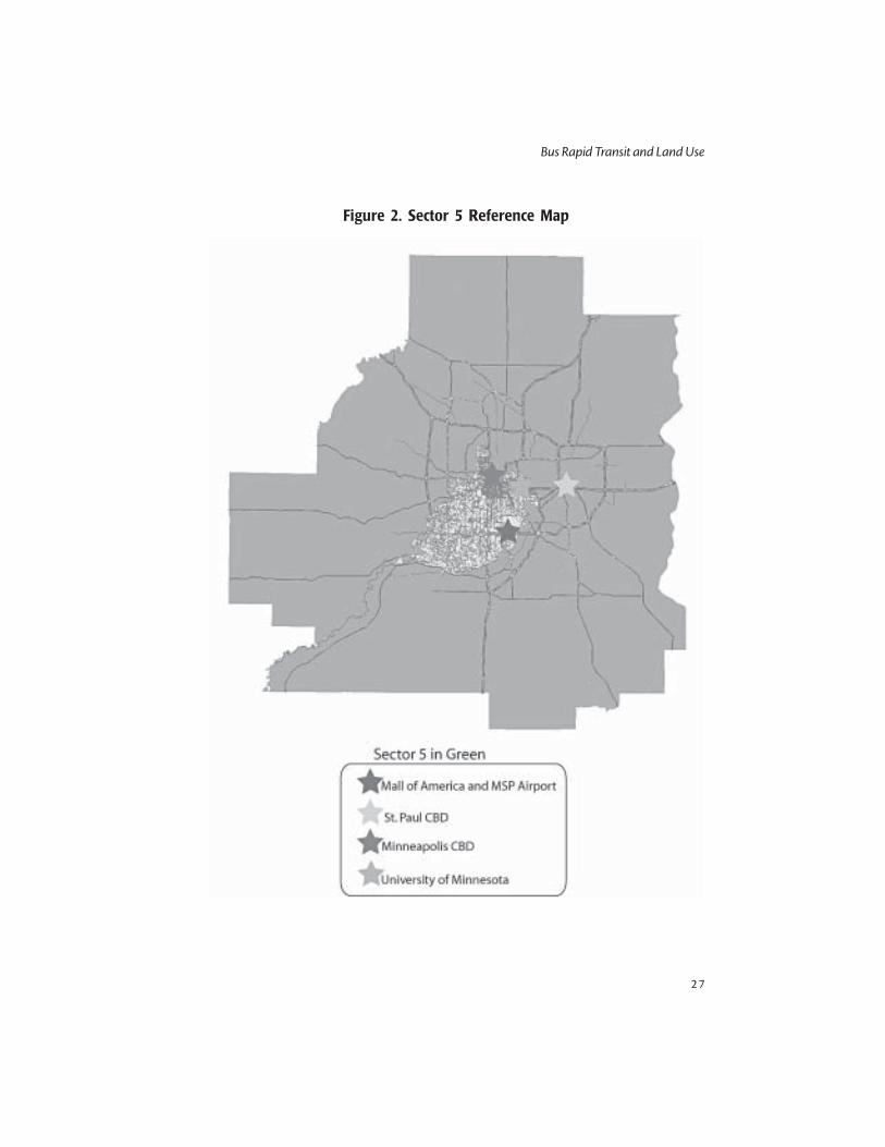
MethodologyThis analysis uses the Sector 5 restructuring data obtained from the MetropolitanCouncil, the regional planning agency for the Minneapolis-St. Paul metropolitanarea. Sector 5 is the transit planning subregion that consists of downtown Minne-apolis and a radial slice running due south and southwest (Figure 2). Sector 5contains four of the primary trip generators in the entire metro region: the Min-neapolis CBD, Mall of America, International Airport, and part of the University ofMinnesota Twin Cities campus. These data count only the downtown boardingsonto buses that serve Sector 5.
The attractiveness of Sector 5 in this analysis primarily lies in its relative importanceand potential for increased service. It currently serves 55 percent of all transitriders, offers 38 percent of all routes, and almost 20 percent of the jobs and resi-dents in the entire region. This is particularly important given the area only com-prises about 10 percent of the geographic area.
The Sector 5 data used for this analysis consist of weekday transit boardings at busstops in Sector 5 south of the Minneapolis CBD and west of the Mississippi River,known as areas B and C of Sector 5 (approximately 95% of all stops in the sector).Bus stops of different routes at the same location have unique ID numbers, whichallowed control of route orientation and service. Only boardings were used dueto the correlation between boardings and alightings; in other words, people starttheir return trip the same place they ended the beginning trip. This assumptionwas affirmed via visual confirmation of boarding and alighting maps and tables.
Bus Rapid Transit and Land Use
2 7
Figure 2. Sector 5 Reference Map

Journal of Public Transportation, Vol. 6, No. 4, 2003
2 8
The data were compiled using GIS to select and join the relevant census and landuse information with the exact location of the bus stop. The data were enteredinto a demand model and analyzed using a linear regression model. The land usedata were simplified by combining open space, roads, and other categories andomitted from the model to allow a comparison of other land uses to relatively“dead” transit uses.
The cross-town routes are controlled for, while the radial routes feature approxi-mately the same levels of parking availability and price. Generally all parking for alldestinations on routes going away from the CBD is free, and all radial routes goingtoward the CBD terminate there.
The use of transit stops as data collection points, as opposed to individual data viatravel behavior surveys, is useful for several reasons. First, transit agencies planroutes based primarily on area statistics. Similarly, land use planning can moreeasily create types of environments that are more conducive to transit ridership,than it can cause people to use transit. Although ideally both would be used, thesmall area level analysis is often overlooked, and potentially more useful to localplanning agencies.
The transit demand model was created to illuminate the intraurban differences,and so many causes of demand were eliminated. For example, macro-level predic-tors on transit certainly affect transit use. Recent evidence shows that much of the12 percent decline in transit ridership in the first half of the 1990s can be attrib-uted to a sluggish economy and low gas prices, while the increased gas prices andburgeoning economy resulted in a 21 percent increase in ridership in the later halfof the 1990s (Pucher 2001). Density, land use, and transit service provide strongerexplanatory power given the complex decision-making process associated withmode choice within a metropolitan region. Because this analysis only looked atone market at one point in time the macro-level predictors were eliminated fromthe analysis. Similarly, parking prices and size of the CBD were left out becausethese aspects are relatively constant in the area of analysis.
The land use data were classified into basic categories: single-family, multifamily,retail–commercial, office, industrial–-utility, mixed-use, and other. The other cat-egory includes open space, roads, and unused/vacant lands or spaces. Interactionvariables were entered to tease out the influence that various mixes have on transitdemand. Land uses were categorized into groups based whether they are primary

Bus Rapid Transit and Land Use
2 9
job-based (office, industrial–utility), shopping-based (retail–commercial), andhousing-based (single-family, multifamily).
FindingsGeographyA majority of the weekday transit demand in Sector 5 is currently located insidethe City of Minneapolis, and more than 12 percent of total boardings in Sector 5occurred in downtown Minneapolis (Table 2). Demand is clustered along LakeStreet in South Minneapolis and peaks at the confluence of other transit routes(Figure 3). The ridership clustered along the Lake Street corridor, featuring cross-town service, is the area of maximum transit accessibility in Sector 5. This area is atmaximum accessibility because route 21 runs the distance of Lake Street, connectsto nearly every radial route in sector 5, and offers very high-frequency service.
Table 2. Weekday Boardings by Location in Sector 5
Transit ServiceThe type of transit service plays a significant role in demand of a given stop (Table3). Compared to the Urban Local service, the most prevalent service in the corearea, Urban Local-Limited Stop was negatively associated with demand (Table 3).Surprisingly the level of weekday service was not a significant determinant of tran-sit demand. To better understand the relationship between transit service andridership, a longitudinal analysis is warranted.
Location Boardings % of TotalMinneapolis City 46964 76.1%
St Paul City 6551 10.6%
Minneapolis Suburbs 7571 13.3%
Total Boardings in Analysis 61697 100.0%
Major Trip GeneratorsMinneapolis CBD 8553 13.9%
Mall of America 838 1.3%
Airport 238 0.4%

Journal of Public Transportation, Vol. 6, No. 4, 2003
3 0
Figure 3. Total Boardings by Bus Stop in Sector 5
Some degree of reverse causality is likely occurring and subsequently, altering thefindings. Transit planning is ideally demand responsive; the direction of causality islikely in reverse. The level of service is altered to more accurately reflect existingdemand and the routes have reached a point of relative equilibrium.

Bus Rapid Transit and Land Use
3 1
Table 3. Linear Regression Model of Transit Demand

Journal of Public Transportation, Vol. 6, No. 4, 2003
3 2
SocioeconomicsAreas of with higher percentages of the population in the 0–16 cohort enjoyhigher transit demand relative to the 30–50 cohort (Table 3). Most likely, peoplewithout a driver’s license must rely on transit service, as they, theoretically, areunable to operate an automobile. Also, these areas are likely to have a larger house-hold size and have lower levels of income available for more convenient transpor-tation (i.e., the automobile).
The percentage of residents with access to an automobile was not surprisinglynegatively associated with transit demand (Table 3). The greater the percentage ofthe population with access to an auto, the more likely someone will drive, espe-cially given that most people enjoy abundant free or inexpensive parking in theTwin Cities. This finding seems particularly troubling given most people have ac-cess to an automobile.
The general lack of significance of socioeconomic variables suggests that some ofthe myths regarding urban public transportation may be easily debunked. Forexample, a general perception exists that transit (especially buses) is for poor peopleand poor areas; however, the evidence here fails to support such a notion. Simi-larly, the model fails to support any notion regarding public transit use as relatedto race/ethnicity, household size, or education.
DensityNearly every study that has focused on transit ridership has provided evidencethat density is the primary determinant of transit ridership (see Seskin and Cervero1996 and Table 1). A study by Nelson/Nygaard (1995) showed 93 percent of thevariation of transit demand in different parts of the Portland region is explained byemployment and housing density, even after controlling for 40 land use andsociodemographic variables. One problem with density is that it is highlyintercorrelated with other variables, as studies that have focused on density areprobably missing everything that comes with it (Handy 1996a).
While population density of the block the bus stop is on is unrelated to transitdemand, population density of the larger block group is significantly related totransit demand (Table 3). Many bus routes run along commercial corridors andso the lower demand associated with density at the block level is likely a result ofadjacent commercial uses and while the residential areas are off the block proper.The significant relationship at the block-group level would support this notion
Bus Rapid Transit and Land Use
3 3
and give further credence that density is of primary importance relative to transitdemand.
Land UseMultifamily residential land use was associated with lower transit demand withinan eighth mile of transit stops, and associated with higher demand from an eighthmile to a quarter mile of transit stops. While the negative association near transitstations is counter to the hypothesis, the positive association within a quarter milegives further credence to the finding that larger densities within the larger areahave stronger implications on transit demand than do high densities adjacent tothe line.
Transit demand is related to the percentage of mixed-use and retail-commercialland within a quarter mile of the bus stop (Table 3). The significance of adjacentvertical mixed uses to transit demand is consistent with the claims of TOD propo-nents and existing literature. The positive association of retail–commercial usesuggests that people use transit for both nonwork and work-related travel or thatemployees of retail–commercial activities are more likely to use transit. Retail use ispositively related to transit demand both within an eighth mile and quarter mileof the transit stop (Table 3).
Land Use Interaction EffectsSome land use interaction is evident (Table 3). The greater the difference betweenhousing-based and employment-based land uses, the lower the demand for tran-sit (Table 3). Jobs–housing balance is believed to be the outcome of a free market,as jobs and housing colocate to maximize access to one another (Cervero 1996).However, there is generally little evidence to support that jobs–housing balanceactually occurs, and secondly, that it has any noticeable impact on transit.
A negative relationship exists between housing–shopping balance and transit rid-ership (Table 3). While this contradicts the standard TOD model, it is consistentwith the standard gravity model. In other words, if shopping opportunities existnearby, there is no need to travel longer distances to reach the same opportuni-ties.
Greater opportunity is considered preferable to most because it reduces the needto travel. However, reducing the need to travel does not necessarily equate to lesstravel. Some people enjoy travel in the automobile (i.e., the culture of cruising);however, there is little evidence that people ride transit in that manner (except for

Journal of Public Transportation, Vol. 6, No. 4, 2003
3 4
tourism). In other words, a greater balance between shopping, housing, and em-ployment-based land uses would seem to lower transit demand.
Future Research DirectionSignificant advances have been achieved in transit/transportation–land use re-search in recent years, but much is left to be desired. Future research of this kindshould focus on determining the catchment areas of the various land uses anddensity variables. The general rule estimates that people are willing to walk a quar-ter mile to transit stations. However, it remains unclear exactly how this assump-tion was estimated and how this number might change based on the quality ofservice and climate differences, as it is unlikely to be a one-size-fits-all application.
Understanding the temporal variation of transit demand would greatly enhancethe ability to provide efficient and effective transit service. Travel behavior litera-ture has created a strong foundation for understanding how people change theirbehavior, including mode choice, based on the time of day that they are able totravel. For example, people may be more likely to visit retail locations via transitbetween the hours of 5 and 7 P.M. during the week, and middle of the afternoonon the weekends. Information such as this, combined with spatial transit demanddata would increase the ability of transit planners to provide the service transit-dependents require, while capturing a larger share of “choice riders,” or those whochoose transit over other modes. This information is particularly useful given thegeneral propensity of government funding toward the auto and auto-orienteduses and lack of funding available for transit.
Another major drawback to transit–land use analyses is the difficulty in measuringland use design and diversity measures. Diversity measures have employed en-tropy measures and a dissimilarity index (Cervero and Kockelman 1997; Frank andPivo 1994), and estimated the distances between several different retail commer-cial uses and residential units (Handy 1996b). While these measures are innovativeuses of existing data, they leave much to be desired . To truly illuminate the com-plex causes of transit demand, a much more robust statistical foundry is needed.Considering the difficulty in funding such comprehensive data collection andentry, and slim funding to transit agencies, large data enhancement is as unlikely asit is necessary. Similarly, researchers have made significant progress onoperationalizing other aspects of land use in recent years (Evans et al. 1997;Loutzenheiser 1997; Cervero and Kockelman 1997; Krizek 2002; Hess et al. 2002).Despite these improvements, highlighting the effect of pedestrian environmental

Bus Rapid Transit and Land Use
3 5
factors (street lighting, sidewalk width, timing of crosswalks, on-street parking) orland use factors (setbacks, presence of front porches, windows facing the front),and possibly even social connectivity (tightness of community, social organiza-tions) could greatly enhance the collective understanding of the effect of designand diversity on travel behavior and transit ridership.
Also, the existing measures fail to address the interaction between different landuses and the effect of interaction on travel behavior and transit use. The use of aheterogeneity measures assumes that every mix is the same, which is inaccurate(Hess et al. 2002). Measuring land use complementarity is an important step to-ward crafting “transit-friendly” land use plans and regulations, as well as testingand increasing the effectiveness of TOD.
Finally, a combination of a cross-sectional and longitudinal analyses, as well asboth area and individual level data, will provide a stronger foundation to predictthe effect changes in service have on ridership and development patterns neartransit stops. In addition, such an analysis would help control for self-selection,and would provide insight toward the effect that various levels of transit servicechange have on residential demand near transit stops.
Conclusions and Policy ImplicationsLand Use ImplicationsThe results of this research suggest there are three primary means available toplanners to enhance transit ridership through land use planning: increase residen-tial density in the areas near transit corridors, concentrate mixed-use develop-ment within an eighth mile of the transit corridors, and channel a greater propor-tion of the retail development within a quarter mile of transit lines. In fact, thisanalysis suggests that transit planners would increase ridership to a greater degreethrough catalyzing retail, mixed-use and multifamily development than increas-ing transit service.
While the results of the model provide support to TOD, some minor changes tothe traditional TOD model are proposed. The clustering of vertical mixed-usesand retail–commercial near transit stops and higher density residential within aquarter mile of transit stops remains consistent with the traditional CalthorpeTOD model. However, existing literature in conjunction with this analysis wouldnot promote office use in neighborhoods, but would rather cluster office uses inthe CBD. Although the model in Figure 4 is crude, it provides a visual representa-tion of the land use findings from this analysis.

Journal of Public Transportation, Vol. 6, No. 4, 2003
3 6
Figu
re 4
. Com
pari
son
of t
he T
radi
tion
al T
OD
Mod
el a
nd M
odel
Res
ulti
ng f
rom
thi
s A
naly
sis

Bus Rapid Transit and Land Use
3 7
Despite the auspiciousness of land use planning as a transit ridership tool, it isdifficult to determine the degree self-selection affects these results. Most likelythose who choose to ride transit choose their residential location based on thatpremise. In other words, changing the land use or density around a given bus stopdoes not necessarily make people in the vicinity more likely to use transit
While substantial improvements are needed in the world of research, even greaterimprovements are needed in the world of practitioners. Those ideas that havebeen reinforced by numerous studies (i.e., intensity of use and limited parkingresult in higher transit ridership) have yet to be implemented by planning agenciesto any significant degree. To increase ridership to the point that an effect oncongestion and the built environment is evident, strong land use planning, invest-ment in transit, and political will are necessary.
Finally, while these results illuminate the causes of transit demand, the effect isquite small. Predicting complex human behavior is a problem that has plaguedthe social sciences since their development. While some of these results are statis-tically significant, they fail to explain much of the variation associated with transitdemand. The result of implementing these results will increase transit demand,but only marginally, which is evident given the small coefficients associated withthese predictors. However, the results, and subsequent policies prescribed, shouldbe weighed in light of the alternatives. The effect of these contributors to transitdemand may be small, but they are better than the continuation of the omnipres-ent auto-oriented environment in the United States.
As urban America becomes increasingly disgruntled with its transportation op-tions, public officials will have their feet held to the policy flame in order to makechanges. At some point politicians and researchers will be forced to convince theAmerican public to change or balance their preferences for accessibility and hous-ing-related amenities. Enhanced research, and putting what is known into prac-tice, will go a long way toward doing so.
Journal of Public Transportation, Vol. 6, No. 4, 2003
3 8
References
Boarnet, M. G., and R. Crane. 1998. Public finance and transit-oriented planning:New evidence from Southern California. Journal of Planning Education andResearch 17: 206–219.
Bureau of the Census. 2000. STF3A summary files. Washington DC.
Calthorpe, P. 1993. The next American metropolis: Ecology, community and theAmerican dream. New York: Princeton University Press.
Cervero, R. 1998. The transit metropolis: A global inquiry. Washington DC: IslandPress.
Cervero, R. 1996. Jobs-housing balance revisited: Trends and impacts in the SanFrancisco Bay Area. Journal of the American Planning Association 62(4): 492–512.
Cervero, R., and K. Kockelman. 1997. Travel demand and the 3 Ds: Density, diver-sity and design. Transportation Research D 2(3): 199–219.
Evans, John E., V. Perincherry, and G. B. Douglas III. 1997.Transit friendliness fac-tor: Approach to quantifying transit access environment in transportationplanning model. Transportation Research Record 1604: 32–39
Ewing, R., and R. Cervero. 2001. Travel and the built environment. TransportationResearch Record 1780: 87–114.
Frank, L. D., and G. Pivo. 1995. Impacts of mixed use and density on utiliation ofthree modes of travel: Single-occupant vehicle, transit and walking. Transpor-tation Research Record 1466: 44–52.
Handy, S. 1996a. Travel behavior issues related to neo-traditional development—A review of the research. Presented at TMIP Conference on Urban Design,Telecommuting, and Travel Behavior. FFWA, U.S. Department of Transporta-tion.
Handy, S. 1996b. Understanding the link between urban form and nonwork travelbehavior. Journal of Planning Education and Research 15:183–198.
Hess, D. 2001. Effect of free parking on commuter mode choice: Evidence fromtravel diary data. Transportation Research Record 1753: 35–42.

Bus Rapid Transit and Land Use
3 9
Hess, P. M., A. V. Moudon, et al. 2002. Measuring land use patterns for transporta-tion research. Transportation Research Record 1780: 17–24.
Krizek, K. 2002. Operationalizing neighborhood accessibility for land use travelbehavior research and regional modeling. Journal of Planning Education andResearch.
Loutzenheiser, D. R. 1997. Pedestrian access to transit: Model of walk trips andtheir design and urban form determinants around BART stations. Transpor-tation Research Record 1604: 40–49.
Nelson/Nygaard Consulting Associates. 1995. Land use and transit demand: Thetransit orientation index, Chapter 3. Primary Transit Network Study. Portland,OR: Tri-Met.
Pucher, J. 2001. Renaissance of public transport in the United States? Transporta-tion Quarterly 56(1): 33–49.
Puskarev, B., and J. Zupan. 1977. Public transportation and land use policy.Bloomington, IN: University Press.
Seskin, S., and R. Cervero. 1996. Transit and urban form. Washington DC: FederalTransit Administration.
About the Author
ANDY JOHNSON ([email protected]) is a long-range transportation planner forthe Oregon Department of Transportation. He is a graduate of the master’s inUrban and Regional Planning program at the University of Minnesota and theCenter for Transportation Studies. Mr. Johnson worked as a planning consultantfor the Ventura Village neighborhood on the Southside of Minneapolis and beeninvolved with transit, land use, and travel behavior research at the University ofMinnesota. He was recently awarded the Barbara Lukermann Service to PlanningAward for his efforts in connecting the planning program to the larger commu-nity.

Journal of Public Transportation, Vol. 6, No. 4, 2003
4 0

Evaluating Urban Commute Experience
4 1
Evaluating the Urban CommuteExperience: A Time Perception
ApproachYuen-wah Li
AbstractAbstractAbstractAbstractAbstract
This article examines the perception of travel time and evaluation of the urbancommute experience. It reviews the literature on time perception in psychology,positing perceived travel time as a function of commute characteristics, journeyepisodes, travel environments, and expectancy. Insights from emerging behavioraleconomics are drawn to illuminate evaluation of the urban commute experience.The perception–evaluation correspondence presents the potential of a new researchapproach to travel behavior. A time perception model for evaluating urban com-mute experience is formulated to accommodate all the posited relationships, withpossible moderations by goal attainment, economic values associated, and timeurgency. Practical significance of the model is exemplified through its use in explain-ing mode choice, and as a guide for service planning and design.
IntroductionLike many other domains of consumer behavior, travel behavior has convention-ally been studied with the approach that treats all (including monetary and tem-poral) aspects of evaluation of a travel experience as a single dimension. A traveleris assumed to view temporal and monetary expenditures alike, and trade one foranother on a compensatory basis. In the transportation literature, this single mea-sure is referred to as the “generalized cost,” and represents the overall utility (or
Journal of Public Transportation, Vol. 6, No. 4, 2003
4 2
disutility) of a given commute. The conventional approach, despite its prevalencein transportation research, has devoted inadequate attention to possible distinc-tive features of temporal experience and expenditures. In consumer research lit-erature, time behavior has received increasing interest over the past decade withthe growth of service industries (Carmon 1991). Yet, most of the studies havebeen conducted primarily with waits (see Durrande-Moreau 1999 for a review)among experiences of time consumption. While waiting time is just one episodeof a travel journey, the temporal experience of an urban commuter over the entirejourney has rarely been examined in sufficient detail.
Given the fact that daily commutes incur a rather substantial amount of temporalrather than monetary expenditures, investigation of commuters’ perceptions ofthe travel time and their evaluation of the travel experiences is justified. This articlediscusses the perceived time (i.e., psychological time) vis-à-vis objective clock timethat one spends in daily commutes, and examines how it relates to the evaluationof one’s travel experience. This proposed research approach is of potential toexpand the extant body of knowledge in travel behavior that rests primarily onutilitarian assumptions. It illuminates the human processes, such as perception,underlying the evaluation of travel experiences, rather than the evaluative out-comes per se. The time perception approach is promising not only because itopens up new venues for transportation research, but also because of its implica-tion for the design and planning of transportation systems and the formulationof transport policy. Advances in knowledge and practice as a result of innovativeresearch approaches should be pursued by transport planners and policy-makerswho have endeavored to promote the use of public transportation while autodominance (ownership and use) has been on the rise during the past decades. It is,therefore, particularly worthwhile to focus the research context on public trans-portation.
This article begins with a brief review of the potential contribution of time percep-tion research to the understanding of a traveler’s temporal experience in dailycommute. Next, findings from the time perception literature are drawn and dis-cussed as pertinent to the specific context of urban commute, with tentativeconclusions proposed in the form of research hypotheses. Then commuter evalu-ation of travel experience, as inspired by the emerging behavioral decision theory,is examined as a way to explore its possible connection to the perception of com-muting time. Based on the tentative conclusions arrived, a framework proposingtime perception to be pivotal to evaluation of daily commute experience is ad-

Evaluating Urban Commute Experience
4 3
vanced to guide future empirical validation and further research. Lastly, summaryand concluding remarks are presented. As public transportation offers the mostdiverse form of urban commute experiences, discussion and tentative conclu-sions are made and drawn with reference to this specific context.
Concepts and Models for Time PerceptionTime perception has a long history in psychology research, dating back to the late18th century (Roeckelein 2000). Research findings have rendered a valuable sourceof reference to the understanding of temporal experience of the daily commute.This article presents a selective review of essential concepts and models from majorcontributors such as Fraisse (1984), Block and Zakay 1996), Boltz (1993), andHornik (1992).
Time PerceptionThe notion of time refers to succession and duration, two different concepts butboth related to one’s experience of change (Fraisse 1984). The concept of succes-sion involves the perception of two or more different and sequentially organizedevents, whereas the concept of duration concerns the interval between two suc-cessive events. Temporal experience refers to an individual’s perceptual physicalchanges, and the duration in perception is measured against a regular sequence ofsuccession. Time perception, according to Fraisse’s conception, is defined as “theattention to, or apprehension of, change through the integration of a series ofstimuli and characterized by the ability to conceive of duration, simultaneity, andsuccession” (Roeckelein 2000, p. 53). It implies that time in perception bears nostraightforward relationships to physical time (Fraisse 1984). Hence, the subjec-tive duration experienced by a traveler may be different from the objective timepassed.
In fact, this conception lies with the major research interest of time psychophysicsthat concerns the psychological magnitude of the passage of time (Grondin 2001).Evidences from the psychophysics literature have suggested perceived (subjective)time as a power function of the objective clock time, which is often referred to as“Stevens’ law” (Roeckelein 2000; Grondin 2001). Growth of the psychologicalmagnitude of a given duration may be faster than, slower than, or equal to growthof the physical magnitude, subject to the exponent value being greater than,lower than, or equal to unity respectively (Grondin 2001). Eisler (1976), for in-stance, concluded an exponent value of 0.9 as the best overall approximate for thepsychological law applied to time perception.
Journal of Public Transportation, Vol. 6, No. 4, 2003
4 4
Contextual-Change ModelSeveral models of psychological time have been advanced in the literature with anattempt to better explain and model psychological time. These models fall intotwo conventions of research: sensory-process convention and cognitive conven-tion (Block and Zakay 1996). The cognitive approach has prevailed research inpsychological time, namely because it offers a more useful way to understandduration experience based on such basic concepts as attention, information pro-cessing, and memory (Block and Zakay 1996; Grondin 2001).
Block’s (1985) contextualistic model, among cognitive models, proposes thatduration experience results from an interaction among:
1. contents of time periods (e.g., empty or filled time);
2. activities during time periods, including temporal and nontemporal at-tentions;
3. subjects’ characteristics (e.g. personality); and
4. temporal behavior (e.g., method of measurement).
Block’s model seems to corroborate Fraisse’s conception of time perception asrelated to contextual changes on the one hand, and has elaborated the effect ofthe contextual changes in terms of attentional processes on the other. Subse-quently, Block and Zakay (1996) advanced the contextual-change model thathighlighted the importance of temporal attention in determining prospectiveduration judgments. According to Block and Zakay’s model, contextual changesare encoded as time-tags in one’s temporal information processing, and hencedirectly influence duration judgment. However, given the scarcity of one’s cogni-tive resource, nontemporal events taken place in the meantime may competewith temporal cues for attention and processing, and affect duration judgment.
The literature on psychological time has also distinguished between prospectiveand retrospective duration judgments or estimations (Block and Zakay 1996;2001). The prospective paradigm refers to the situation in which participants areaware of being engaged in a duration estimation task. Participants may encodetemporal information as part of the experience of the time period, and so theirjudgment is referred to as an “experienced duration.” On the other hand, in theretrospective paradigm, participants have no prior knowledge of the durationjudgment task. When asked afterward about the duration, participants may re-trieve whatever information available in memory. Their judgment is referred to as

Evaluating Urban Commute Experience
4 5
a “remembered duration.” As most urban commutes (e.g., going to work) aremade regularly, and draw one’s attention and estimation of the time spent some-how, the prospective paradigm should be appropriate for the task of judging anexperienced duration of commute.
Temporal and Situational EnvironmentsCorroborating Fraisse’ (1984) conception of time as the succession of events overa period, researchers such as Boltz and her colleagues (e.g., Jones and Boltz 1989)have advocated that the structure of events constitutes the temporal environ-ment of duration judgment tasks. The temporal pattern of events (usually in theform of nontemporal information) over a period of time affects the way individu-als attend to the events, and thus their determination of duration estimates. Highlycoherent events present structural predictability over an arbitrary time span, andhence conducive to future-oriented attending, whereas lowly coherent eventscontain little predictability, and hence conducive to analytic attending. Individualsadopting future-oriented attending will seek higher order time patterns and gen-erate expectancies about the start and end of a series of events, whereas thoseadopting analytic attending will turn to adjacent events in organizing ill-struc-tured information. Therefore, in duration judgment tasks, the former group willbe biased by the disconfirmation of expected (starting or ending) times, and thelatter group by their attention to the amount of local details. Urban commutes ofa daily or regular practice should be more conformed to events of high coherence,and so individual travelers are likely to adopt future-oriented attending in theirperception of the commute time consumed.
On the other hand, the consumption and perception of time is also situationbound (Hornik 1982; 1984; 1992). Hornik’s (1992) research evidence focuses onthe effect of affective moods as a situational variable on temporal judgment. It ishypothesized that mood biases temporal judgment by influencing the informa-tion to be recalled from memory. Individuals in a good (bad) mood, for instance,are prone to retrieve positive (negative) information, which in turn biases theirjudgment in a direction congruent with the mood. Alternatively, their judgmentmay be conceived as a direct consequence of the affective responses, positive ornegative, to the stimuli under investigation. Urban commuters moving throughhassles of various kinds are liable to fluctuating affective states that influence theirtemporal judgment of the commute.

Journal of Public Transportation, Vol. 6, No. 4, 2003
4 6
Time Perception in an Urban Commute ContextIt is hypothesized in this article that the perceived travel time of urban commuters(presumably with public transportation) varies with commute characteristics,journey episodes (i.e., ride, wait, access and transfer, service environments), andtheir expectancies. These relationships are discussed below, making reference tothe insights from the time perception literature. The discussion is summarized inthe form of research propositions as shown in Table 1.
Table 1. Summary of Propositions for Perceived Travel Time
Evaluating Urban Commute Experience
4 7
Commute CharacteristicsCommute characteristics include commute duration and commute stage.
Commute Duration
Dating back to the 19th century, Vierordt, among the pioneers of time psy-chophysics, conducted experiments on time judgment. His observations arereferred to as Vierordt’s law (Roeckelein 2000). One conclusion is that “for allcategories of time from seconds to years, the same law holds good (i.e., rela-tively short intervals are lengthened by judgment, and relatively long intervalsare shortened” [p. 73]). In regard to a commute experience, a traveler will finda short commute duration longer, whereas a long commute duration shorter,compared to the objective clock-time measurement. This implies that com-mute duration per se biases the commuter’s perceived duration.
Commute Stage
Urban commuters, particularly those using public transportation, are usedto journey interrupts of various kinds (e.g., making transfers in the middle ofa trip). These interrupts may be conceived as dividing a single journey intomultiple commute stages. Fraisee’s principles (Roeckelein 2000) provide in-sights into the understanding of the effect of staged journeys on perceivedtravel time. The principles state:
1. A divided interval of time appears to be longer than an empty (standard)interval of the same duration.
2. An interval of time with more divisions appears longer than one withfewer.
3. Of two divided intervals, the one that is evenly divided appears longer thanthat which is irregularly divided. (p. 124–125).
The first principle supports the prediction that travelers perceive a given com-mute experience as being longer, when the journey has more commute stages.In other words, from the commuter’s perception, interrupts over a journeyare time consuming. Fraisee’s second principle further suggests that the morecommute stages (e.g., transfers) a journey requires, the longer the travel timewill be perceived. The third principle, on the other hand, reveals how thedistribution of interrupts affects one’s experienced duration of a journey. Itsuggests that, given the same number of interrupts as required by a journey,travelers subject to more evenly distributed stages perceive the travel time as

Journal of Public Transportation, Vol. 6, No. 4, 2003
4 8
being longer. To illustrate, all else being equal, travelers perceive a given two-staged journey comprising two equal-duration segments as being longer,than a short (long) duration segment followed by a long (short) durationsegment.
Journey EpisodesAccess, wait, ride, and transfer characterize the episodes of urban commute expe-rience, particularly with public transportation. Perceived duration, however, islikely to vary across the episodes in the light of the relative attention to temporaland nontemporal information (Block and Zakay 1996) and the likely affectivestate elicited (Hornik 1992) in particular episodes. A description of the generalexperience in each commute episode follows.
Ride
Given a reasonably stable and comfortable environment, urban commutersin ride episode are likely to be engaged voluntarily or involuntarily in activitiessuch as scheduling daily jobs, reading, day dreaming or napping, and chattingwith friends (in person or on phone). These activities demand either a consid-erable amount of cognitive resource or high involvement by commuters,thus substantially undermining the chance of temporal information process-ing. The taking place of these activities in concurrence with one’s commutecharacterizes the polychronic time use (i.e., “two or more activities are per-formed within the same time block, apparently at the same time”) (Kaufman,Lane, and Lindquist 1991, p. 393). That is, riding in a setting of reasonablecomfort is conducive to polychronic time use which shortens the perceivedduration of travel. Urban commuters in ride episode, compared to otherjourney episodes, are likely to experience the fastest pace of time passage andperceive a given duration as being the soonest.
Wait
Travelers on wait (e.g., for bus service) are subject to unoccupied time, andthus very attentive to the passage of time (Block and Zakay 1996). Temporalcues embedded in the wait context (e.g., repeated passing of unintended busservices or frequent time-checking behaviors by travelers in the same queue),will easily elicit the traveler’s temporal attention and temporal informationprocessing. Moreover, the waiting experience will expose travelers to an unful-filled goal. A discomfort or dissatisfying mood may lead to overestimation ofthe traveler’s temporal judgment. In combination of these effects, urban com-

Evaluating Urban Commute Experience
4 9
muters in wait episode are plausibly perceiving a given duration as being thelongest among the journey episodes.
Access and TransferTravelers in access or transfer for public transportation will be required toaccomplish nontemporal tasks, such as walking, looking for guides, and mak-ing their way out of a moving crowd. Subject to the scarcity of cognitiveresources, travelers may be inattentive about temporal information, thus notnoticing time passage. However, unlike riding on board, access or transferrequires efforts that cannot free travelers for other activities of their choice.Furthermore, travelers may find dealing with access or transfer a stressful task,particularly with an unfriendly arrangement or setting. The negative affectthus aroused may bias the perceived duration upward. As a consequence,urban commuters are likely to perceive a given duration in access or transferepisode as being longer than in ride episode, though shorter than in waitepisode.
Travel EnvironmentGiven the fact that both temporal attention and affect are context dependent,perceived travel time is subject to an array of environmental factors. The effect ofcomfort and entertainment provided along the journey episodes are examinedbelow.
Comfort
Comfort has been widely reported in the literature as one of the key dimen-sions of customer satisfaction for public transportation (see Li 2001 for areview). It is a composite measure of attributes related to service environ-ment, including but not limited to seat availability, smoothness of rides, spa-ciousness (or loading), air-conditioning (or ventilation), lighting, cleanliness,spatial layout, and furniture and facilities design. A comfortable and pleasantcommute environment is, on the one hand, conducive to polychronic timeuse, and on the other hand, of benefit to mitigate commuting stress and thenegative emotions elicited. These effects in combination lead to underestima-tion of one’s temporal judgment.
Entertainment
Entertainment is provided in commute environments, as in many service set-tings, as a time filler to direct customer attention to the nontemporal stimuli

Journal of Public Transportation, Vol. 6, No. 4, 2003
5 0
presented so as to undermine temporal information processing. Moreover,amusing entertainment is able to elicit positive moods during one’s com-mute. These effects altogether appear to be conducive to shorten perceivedtravel time of urban commuters. However, the use of time fillers (e.g., visualand audio entertainment, and music broadcasting as commonly used in publictransportation) can lead to mixed results. Entertainment containing overlyrepetitive or perpetually familiar content has been shown to lengthen one’sperceived duration (Kowal 1987), when presenting as temporal cues, or in-ducing boredom, or both. Also, customer affective responses to musical piecesvary with individual tastes and preferences (North and Hargreaves 1999).
ExpectancyUrban commute, regardless of the transportation mode used, is likely to be ha-bituated through repeated practice as a routine activity. Conceiving the daily rou-tine as a series of highly coherent events, urban commuters may have adoptedfuture-oriented attending, and generated certain temporal expectations or pre-dictions (Jones and Boltz 1989) for the duration normally required for each jour-ney episode and the journey as a whole for instance. Research by Boltz (Jones andBoltz 1989; Boltz 1993) has indicated that departures from one’s temporal expec-tation led to biased temporal perception. Therefore, urban commuters perceive agiven duration of travel as being longer (shorter) if the duration is longer (shorter)than expected, that is when the expectation is negatively (positively) disconfirmed.
In a relatively unstable commute environment (e.g., frequent road congestion forcar commuters or public transportation with frequent delays), travelers may havedifficulty apprehending temporal expectancy, making the commute an uncertaintask. Given the correlation between task uncertainty and overestimated duration(Boltz 1998), an urban commute taking place in a rather unpredictable setting isexpected to result in longer perceived journey time.
Evaluation of the Urban Commute ExperienceTraditional decision theory presumes people make choices based on “decisionvalue” (i.e., the predicted outcome for future experiences with perfect accuracyand option evaluation) (Kahneman and Tversky 1984). Emerging behavioral eco-nomics, in contrast, recognizes the important role of “experience value” in thedecision-making process. It assumes decision-makers to be hedonic and con-cerned about “the degree of pleasure or pain, satisfaction or anguish in the actualexperience of an outcome” (p. 170), instead of being utilitarian and concerned

Evaluating Urban Commute Experience
5 1
about the anticipated outcome. In this article, evaluation refers to the “experiencevalue” that commuters rate toward a given urban commute experience. The fol-lowing sections examine evaluation of the urban commute experience by com-mute characteristics, journey episodes, and expectancy. The extant body of litera-ture on behavioral economics, particularly the Prospect theory (Kahneman andTversky 1979), is taken as the primary source of reference, with support from thefindings of transportation research where appropriate. Tentative conclusions aresummarized as propositions in Table 2.
Table 2. Summary of Propositions for Evaluation of the UrbanCommute Experience
Journal of Public Transportation, Vol. 6, No. 4, 2003
5 2
Commute Characteristics
Commute Duration
The Prospect theory suggests that value is assessed with respect to gains orlosses, and the value function generally exhibits a concave shape in the gaindomain and a convex shape in the loss domain (Kahneman and Tversky1979). To the extent that commuting time is considered a loss, the valuefunction of commute duration is expected to exhibit convexity. Otherthings being equal, the experience value for a given urban commute isexpectedly subject to diminishing sensitivity of the total travel duration: thelonger (shorter) the commuting time, the lower (higher) its marginal value.Findings from the transportation research literature also lend support tothe convexity of the value function of commute duration (e.g., Kjoerstadand Renolen’s [1996] valuation of travel time in five Norwegian towns, andSmall and colleagues’ [Small, Noland, Chu, and Lewis 1999] willingness topay study for reduced congestion delay for various trip lengths in theUnited States).
Commute Stages
Travelers making a multistaged journey may be conceived as subject tocombined prospects, in which losses are segregated by commute stages(Kahneman and Tversky 1979). Given a convex loss function, the segregatedlosses in accumulation shall loom larger for a multistaged journey, com-pared to an equivalent journey of no or fewer commute stages. Further-more, for a constant number of commute stages over a journey, thesegregated losses in accumulation will be greater if those stages are moreuniformly distributed temporally. Though these predictions are by andlarge consistent with the decision behavior based on monetary evaluation,urban commuters as consumers of time are expected to demonstrate aneven stronger propensity to integrate losses (Leclerc, Schmitt, and Dube1995), say by reducing the number of commute stages. Kjoerstad andRenolen (1996) reported a strong preference for direct trips withouttransfer, even if the journey time was longer. In two Norwegian cities, directconnection without transfer was rated 1.8 to 5.0 times as valuable for ajourney requiring a transfer with a 5-minute waiting time, or 2.5 to 9.2times as valuable for the one with a transfer with 10 minutes waiting time.

Evaluating Urban Commute Experience
5 3
Journey Episodes
Peak Episode
Kahneman’s research (1999) notes that “retrospective evaluations ofaffective episodes are strongly influenced by the affect experienced atsingular moment” (p. 2). As far as urban commute experience is concerned,some singular moments along the journey episodes may be more affect-laden than the others (e.g. ride without seats, waiting on-streetunsheltered). These instances are likely to arouse strong negative affect, andreturn the most regretful value (i.e., the greatest loss) to the commuters,characterizing “the most extreme affect experienced” (p. 6) moment(s) orthe “peak” snapshot(s) of a journey. For instance, in six Norwegian towns,travel time standing was found to be very “expensive”—rated 2.0 to 3.0times as undesirable for travel time seated (Kjoerstad and Renolen 1996).Walking access, waiting, and transfer were rated 2.0 to 2.5, 1.5 to 3.4, and1.3 to 2.9 times, respectively, as undesirable for travel time seated. Recentresearch studies for the United States revealed the value of out-of-vehicletimes to be 2 to 3 times of that of in-vehicle times (U.S. Department ofTransportation 1997; Bhat 1998), remaining in order with study findingsreviewed in Cherlow (1981). Riding with discomfort and out-of-vehicleepisodes, such as wait or access, are likely to be the peak experiences duringan urban commute.
End Episode
On the other hand, evaluation as to whether the journey’s goal can beattained will usually be processed near the end of a trip. This near-endevaluation may again lead to an extreme affect as at the peak episode,characterizing the “end” snapshot of a journey (Kahneman 1999). Forexample, failing to get to work on time is very likely to elicit a commuter’sintense negative mood. Such strong emotion can overwhelm one’s evalua-tion of the commute, and the entire journey may be viewed as being overlynegative, even though all previous episodes are satisfying. The end-episodeeffect may offer partial support to the notion of higher willingness to payfor more reliable arrival time to work than nonwork trips in the UnitedStates (Small et al. 1999).
Duration Neglect
The “peak” and “end” snapshots, as Kahneman (1999) suggested, determinethe overall evaluation of a given experience, and undermine the significanceof the experience duration. This undermining is referred to as “duration

Journal of Public Transportation, Vol. 6, No. 4, 2003
5 4
neglect” in the behavioral decision literature. Duration neglect suggeststhat, given the intense emotionality of certain singular moments along ajourney, the duration is likely to be negligibly valued, if not totally neglected,in one’s evaluation. Ariely and Carmon (forthcoming) recently set out twoconditions for duration neglect to be in place:
1. when the duration as an attribute is not attended to; and
2. when the duration of the experience is inherent to the experience.
Though duration is inherent to urban commute experience, commuters will some-how care about the duration (e.g., for scheduling or comparing services). It istherefore unlikely that duration neglect will take place in full range in the urbancommute context.
Expectancy
Commuter Reference
As mentioned above, through repeated practice, urban commuters havegenerated certain temporal expectancies. These expectancies are encoded ina commuter’s mental account as costs for routine (temporal) transactions,rather than occasional losses (Thaler 1985). They serve as a reference contextfor one’s assessment of temporal gains (time saved) or losses (time wasted).Given the S-shape of the value function about a given reference point(Kahneman and Tversky 1979), temporal losses shall loom larger thantemporal gains with reference to a commuter’s expectation.
Commute Reliability
Prospect theory (Kahneman and Tversky 1979) predicts that decision-makers rate the importance of sure gains as more valuable than probable(i.e., uncertain) gains, contrasting traditional decision theory that assumesevaluation based on expected value criteria. Leclerc, Schmitt, and Dube(1995) further contend with empirical evidence that individuals are morehighly risk averse toward temporal resources, compared to monetaryresources. One reason given is the low transferability of temporal resources.The certainty effect in regard to temporal resources will be considered moreappealing than monetary resources. As for the urban commute, thecertainty effect is likely to imply a disproportionately high value attached toa stable commute, be it a reliable service (in terms of punctuality andadherence to schedule for instance) or a flow traffic. The predictabilityassociated with a stable commute allows urban commuters to plan how touse their temporal resources more effectively. Kjoerstad and Renolen’s

Evaluating Urban Commute Experience
5 5
(1996) report revealed that passengers in Oslo, Norway, had strong prefer-ences for highly reliable services, and considered even short delays a prob-lem.
Time Perception Model of Evaluating the Urban CommuteExperienceCorrespondence Between Perception and EvaluationThe propositions set out for time perception in the urban commute context andtemporal evaluation of the urban commute experience are outlined and com-pared in Table 3. The comparison exhibits high correspondence between the twoproposition sets. The correspondence reminisces the psychological origin of theemerging behavioral economics, particularly the Prospect theory. The S-shapedvalue function, for instance, seems to reverberate Stevens’ power law as proposedin the psychophysics literature (Roeckelein 2000).
Table 3. Comparison of Propositions Sets for Perceived Travel Time andEvaluation of the Urban Commute Experience

Journal of Public Transportation, Vol. 6, No. 4, 2003
5 6
Furthermore, the correspondence suggests a more coherent relationship withone’s evaluation for the perceived rather than the physical stimuli, despite thedeparture of the perceived reality from the physical reality which Tversky referredto as “perceptual illusion” (McFadden 1998). In other words, subjective time,however illusive, may be rather informative of one’s evaluation of a commuteexperience, as compared to the objective clock time. In fact, research studies onwaiting times have offered consistent evidence for the connection of increasedperceived (wait) time with more negative customer evaluation (e.g., Katz, Larson,and Larson 1991; Pruyn and Smidts 1998; Antonides, Verhoef, and van Aalst 2002).
The ModelThis section discusses the development potential of a research approach to com-mute behaviors that places perceived travel time as central to one’s evaluation of acommute experience. A tentative model is proposed, linking the hypothesizedfactors to one’s perception of travel time, and hence commute experience evalua-tion, as represented by the black solid lines in Figure 1. More specifically, perceivedtravel time is expected to vary with four factor categories:
1. commute characteristics (objective duration and number of commutestages);
2. journey episodes (e.g., commuters are riding or transferring);
3. service or commute environment (comfort and the provision of enter-tainment or the quality of entertainment provided); and
4. expectancy (commuter expectancy and service reliability).
Furthermore, the perceived travel time determined is expected to be predictive ofone’s evaluation of the commute experience.
Despite the postulated importance of perceived travel time to commute experi-ence evaluation, the proposed model accommodates potential direct impacts ofthe identified factor categories on a commuter’s evaluation. These direct contri-butions may be conceived as support for the notion of duration neglect as dis-cussed above. The model, however, leaves open for empirical evaluation the ques-tion as to the extent of explained variances on the commute experience evaluationto be accounted for by the four factor categories with and without the mediationof perceived travel time.

Evaluating Urban Commute Experience
5 7
Moderators for Perception–Evaluation LinkThere may be other constructs at play (e.g., goal attainment, economic values,time urgency) that influence commuters’ perceptions, or moderate the percep-tion–evaluation link, as represented by the dotted lines in Figure 1.
Goal Attainment
As mentioned above, goal attainment is usually assessed near the end of thejourney, and the assessment will possibly bring about intense emotions thatmoderate the perception–evaluation link. On the other hand, as the goal ofmost urban commutes is associated with production or economic activities(e.g., going to work), goal attainment is related to economic gains or losses,which lead to corresponding changes in experience value.
Figure 1: Time Perception Model of Evaluating the UrbanCommute Experience

Journal of Public Transportation, Vol. 6, No. 4, 2003
5 8
Economic Values
The economic costs or values associated with a commute also influence acommuter’s evaluation. For one, fare represents the monetary payoff for thechosen public transportation modes. Wage reflects the economic cost of thetime consumed, as most economists assumed (e.g., Becker 1965). Part of theeconomic values may also be related to goal attainment (e.g. monetary pen-alty for late-comers). Antonides et al.’s work (2002) presents the moderatingeffect of monetary cost of time on the perception–evaluation link for a tele-phone wait setting.
Time Urgency
While perception and evaluation involves subjective judgment of individualcommuters, individual differences should have their part to play. In particular,time urgency as a personality trait or a personality state (Koslowsky, Kluger,and Reich 1995) is expected to affect time perception and experience evalua-tion of individual commuters. As a personality trait, time urgency refers to anindividual’s disposition about time in general (e.g., Type A behavior), whereasas a personality state, it reflects specific time demands of the external environ-ments (e.g., getting to work on time).
ImplicationsExplaining Modal ChoiceThe postulated time perception model is of potential contribution to a betterunderstanding of travel behavior, such as the notion of auto dominance and thepreference for bus over rail as exemplified below.
Auto Dominance
The private car has remained the prevailing mode of transportation for theurban commute. In 1995, the automobile accounted for 43 percent of pas-senger kilometers worldwide (Pucher 1999). The time perception model ofcommute evaluation may well explain the notion of auto dominance in re-gard to a commuter’s perception of travel time. An auto commute is attrac-tive in most courses of perceived travel time, compared to a public transpor-tation commute. It is most likely a door-to-door service, thus minimizing thenumber of commute stages. It spends time predominantly on the ride epi-sode, usually with seats secured and even entertainment (e.g., music) of thecommuter’s choice. It demands the commuter’s (i.e., driver’s) continuous

Evaluating Urban Commute Experience
5 9
attention to road conditions and motor operation, rather than temporalcues or information, and hence exploits the cognitive resource for nontemporalinformation processing. Also, it avoids the temporal and monetary losses dueto unreliable public transportation services. All these may result in a givenjourney perceived as shorter for an auto commute, and hence the commuteexperience to be more positively evaluated than for a commute with publictransportation. Though people intending to travel by car to save time are notnecessarily objectively justified, their savings in the experienced time and posi-tive evaluation associated may be arguably real (Hjorthol 2001).
Bus Versus Rail
Of the public transportation modes, bus and coaches are the most preferred.In 1995, bus and coaches recorded a 20 percent modal split of the world’spassenger transport in terms of passenger kilometers, compared to only a 6percent split for rail-based modes (Pucher 1999). The notion of a larger modalsplit for bus than rail remains valid for well-developed countries such as theUnited States, where modal shares (in passenger-miles) of bus and rail were1.1 percent and 0.5 percent, respectively, in 1997. Though there are manyreasons (e.g., the investment required) to the relative prevalence of bus overrails, the time perception model potentially offers a good account. For in-stance, bus is usually more accessible than rail and is likely to entail fewercommute stages or transfers for urban commuters. On the other hand, bus ismore likely to offer commuters with seats than is rail, and hence more condu-cive to polychronic time use (Kaufman et al. 1991). Therefore, though theobjective travel time for a given journey may be longer for bus than rail, theperceived travel time can be shorter for a commuter with bus than rail, lead-ing to a more desirable evaluation of the bus mode. The reliability of busservices, however, is more susceptible to road conditions, and in some casesrenders bus to be less preferred than rail in view of possible temporal andmonetary losses as a result of service delays.
Guiding Service Planning and DesignThe proposed time perception model of evaluating commute experience is in-tended not only to provide a better understanding of urban commute behaviors,but also to be of practical value to the planning and design of a public transporta-tion system. Of the potential contributions, it highlights perceptual vis-à-vis physi-cal aspects in service planning and design for public transportation. The conven-

Journal of Public Transportation, Vol. 6, No. 4, 2003
6 0
tional approach to service planning design has been obsessed with such efficiencycriteria as maximum flows and shortest paths (travel durations). The proposedapproach, however, calls for the creation of commute patterns conducive topolychronic time use, and the provision of reliable services and a pleasant travelenvironment. It also lends support to the potential of developing walking as adesirable transportation mode.
Transfers
Most public transportation networks are designed with an overwhelmingconcern on efficiency, resulting in transfer points of various kinds for intramodalor intermodal connections. It is inevitable that, in their journey with publictransportation, urban commuters go through more than one commute stage,and experience the transfer episode(s). The tolerance of urban commuters inregard to the number of transfers required, and their temporal distribution,over a journey, however, has yet to be determined. Obviously, travel disruptedby frequent transfers hampers commuters’ polychronic time use. Travel re-quiring a transfer midway keeps commuters attentive for half of the journeyand the related temporal information. It appears, for instance, that the num-ber of transfers required for a journey to work should be limited to two,though more transfers may be acceptable for commutes of other purposes(e.g., leisure). On the other hand, a congenial design of transfer points re-duces the extent of perceived contextual changes, and hence the perceivedpassage of time during the transfer episode. Transfer points so designed, amongothers, may require just a brief access from one line (mode) to another, andhave an integrated in and out for all modes available.
Reliable Services
The time perception model suggests that unreliable or disconformed servicesare evaluated as extremely undesirable by urban commuters, because the traveltime is perceived as unreasonably long. The negative evaluation is likely to becoupled with failure in goal attainment, for instance, due to delayed arrivals.This is in contrast with the auto commute experience in which, under normalroad conditions, the driver has control over the departure time, route choice,speed used, and even the arrival time, as conformed with the commuter’sexpectation. The comparative disadvantage on commute reliability or pre-dictability of public transportation may be one reason that continues tomotivate urban commuters to use autos. Service reliability is, therefore, ex-

Evaluating Urban Commute Experience
6 1
tremely important in attracting urban commuters to public transportation,though not equally important in drawing auto commuters. However, trans-port operators obsessed with efficiency are tempted to publicize the bestachievable service level or the shortest travel time, ignoring the adverse impactof variability on commuters’ perceived duration and service evaluations.Whereas, planners having regard to perceptual elements should seek to man-age commuters’ expectations, say by presenting realistic or rather conserva-tive estimates of service information on the one hand, and give variability adisproportionate weight in service planning and design on the other.
Travel Environment
A comfortable and pleasant travel environment is conducive to polychronictime use, and reduces commute stress and hence a negative mood. Such anenvironment helps to shorten perceived travel time, and bring about positiveevaluation of the commute experience. In regard to the determination ofservice levels for public transportation, for instance, planners overwhelmedwith doing more for less are tempted to pack as many passengers in a givencompartment as the safety requirement would allow at the expense ofcommuter’s experiences. However, it is recommended to establish target loadlevels for different periods of operation that balance efficiency and perceptualconcerns. On the other hand, congeniality, suggested as the guiding principlefor the design of transfer points, should also be adhered to wherever possiblein the design of other commute environments (e.g., wait and access areas). Itencompasses the logistic aspects as well as perceptual factors such as tempera-ture and color tones. It should be noted that while entertainment in publictransportation settings is intended to distract commuters’ attention fromtemporal information, reaction toward the entertainment used, be it visualor audio, depends very much on individual taste. Thus, the effect is ratherunpredictable. A boring film, for example, may be a driver to attend to timepassage, or to go napping while traveling. It is, therefore, difficult to generalizethe use of entertainment as a tool for managing perception.
Walking as a Mode
Walking as a nonmotorized transport mode accounted for 17 percent pas-senger kilometers made among the world’s passenger transport in 1995(Pucher 1999). Walking has met with increasing recognition by policy-makersas an important transportation mode in both the United States and Euro-

Journal of Public Transportation, Vol. 6, No. 4, 2003
6 2
pean countries. While the time perception model suggests that a short com-mute is likely to be perceived as longer, walking presents potential to reduceperceived travel time particularly well for relatively short-distance travels, saywithin 800M. Unlike commutes with public transportation, walking demandsthe traveler’s continuous attention to the environment and motor opera-tion. This may help divert a traveler’s attention from temporal information tonontemporal goals (e.g., a certain building ahead), thus reducing the per-ceived duration of travel. On the other hand, walking, like an auto commute,allows travelers (commuters) to control departure time, route choice, andarrival time, possibly leading to conformed expectation in travel time. It isequivalent to, and as valuable as, a highly reliable transportation mode, par-ticularly for short-distance travels. However, the walking environment pro-vided, including facilities (e.g., air-conditioning), traffic priority, pedestriansafety measures, etc., is essential to promoting walking as a desirable alterna-tive mode. Policy-makers in this pursuit should endeavor to create a pleasantand safe walking environment.
Summary and Concluding RemarksThis article has attempted to contribute an alternative approach to the research oftransportation behavior which has been drawing predominately on conventionaldecision theory and particularly random utility models. It examined the subjectiveperception of travel time spent for the urban commute and evaluation of thecommute experience. In view of the long history of time perception in psychologyresearch, the time perception literature was reviewed, particularly psychophysicsand cognitive models of time perception, as pertinent to the context of the urbancommute. Through the literature review, perceived travel time of urban commut-ers was hypothesized to be contingent with (1) commute characteristics (dura-tion and the number and distribution of commute stages); (2) journey episodes(ride, wait, and access and transfer); (3) travel environments (condition of com-fort and entertainment provided); and (4) expectancy (commuter expectationand commute reliability).
The article has also made reference to the emerging behavioral decision theory,particularly Kahneman and Tversky’s Prospect theory, in the examination of theevaluation of the urban commute experience. It appeared that (1) asymmetricand segregation effects was relating evaluation to commute characteristics; (2)peak-end effect and duration neglect (less likely though) were at play to affectevaluation through journey episodes; and (3) reference and certainty effects ac-

Evaluating Urban Commute Experience
6 3
counted for the impact of commuter expectation and commute reliability onevaluation. Furthermore, the hypothesized relationships exhibited high corre-spondence with those identified for perceived travel duration. A time perceptionmodel of evaluating urban commute experience was proposed, accommodatingall the posited relationships, and placing perceived travel time as central to theevaluation of a given urban commute experience. Some possible moderators forthe link between perceived travel time and evaluation were also postulated anddiscussed, namely goal attainment, economic values associated, and time urgency.
The proposed model not only suggested an innovative approach for transporta-tion research, but also to be of descriptive and prescriptive value for practitioners.It was applied to explain mode choice behaviors, namely auto dominance and thepreference of bus over rail, from the perspective of perceived duration. Moreimportantly, it drew the attention of transport planners and policy-makers to theperceptual vis-à-vis physical aspects of transportation system. Transfers, servicereliability, travel environment, and walking as a transport mode were highlightedand discussed.
Some limitations of this article are acknowledged. The literature reviewed was byno means exhaustive of the total body of the research in psychology and behav-ioral economics. Also, research studies adopting the behavioral economics ap-proach to the investigation of transport behavior are parsimonious. This articlemay be among the few of its kind. In addition, the hypothesized relationships ofthe model are tentative, and yet to be confirmed by empirical evaluation. Thereshould be much room for modification and development based on the result ofempirical examination. Apparently, it is remote to apply behavioral decision theoryto inquire transport choice behavior, to the same extent as conventional decisiontheory is applied. Despite these limitations, this article hopefully presents a pio-neering attempt.

Journal of Public Transportation, Vol. 6, No. 4, 2003
6 4
References
Antonides, G., P. C. Verhoef, and M. van Aalst. 2002. Consumer perception andevaluation of waiting time: A field experiment. Journal of Consumer Psychology12 (3): 193–202.
Ariely, D., and Z. Carmon, Z. Forthcoming. Summary assessment of experiences:The whole is different from the sum of its parts. In G. Loewenstein, D. Readand R. Baumeister, eds., Time and Decision: Economic and Psychological Per-spectives on Intertemporal Choice. NY: Russell Sage Foundation Press.
Becker, G. 1965. A theory of the allocation of time. The Economic Journal 75: 299,493–517.
Bhat, C. R. 1998. Accommodating variations in responsiveness to level-of-servicemeasures in travel mode choice modeling. Transportation Research, A 32 (7):495–507.
Block, R. A. 1985. Contextual coding in memory: Studies of remembered dura-tion. In J. A. Michon and J. L. Jackson, eds., Time, mind, and behavior. Hillsdale,NJ: Erlbaum, p. 1–35.
Block, R. A., and D. Zakay. 1996. Models of psychological time revisited. In H.Helfrich ed., Time and Mind. Kirkland, WA: Hogrefe & Huber, 171–195.
Block, R. A., and D. Zakay. 2001. Retrospective and prospective timing: Memory,attention, and consciousness. In C. Hoerl and T. McCormack, eds., Time andMemory: Issues in Philosophy and Psychology. New York: Oxford UniversityPress, 59–76).
Boltz, M. 1993. Time estimation and expectancies. Memory and Cognition 21 (6):853–863.
Boltz, M. 1998. Task predictability and remembered duration. Perception and psy-chophysics 60 (5): 768–784.
Carmon, Z. 1991. Recent studies of time in consumer behavior. Advances in Con-sumer Research 18: 703–705.
Cherlow J. R. 1981. Measuring values of travel time savings. Journal of ConsumerResearch 7: 360–371.
Durrande-Moreau, A. 1999. Waiting for service: Ten years of empirical research.International Journal of Service Industry Management 10 (2): 171–189.

Evaluating Urban Commute Experience
6 5
Eisler, H. 1976. Experiments on subjective duration 1878–1975: A collection ofpower function exponents. Psychological Bulletin 83: 185–200.
Fraisse, P. 1984. Perception and estimation of time. Annual Review of Psychology 35:1–36.
Grondin, S. 2001. From physical time to the first and second moments of psycho-logical time. Psychological Bulletin 127 (1): 22–44.
Hjorthol, R. 2001. Gendered aspects of time related to everyday journey. ACTASociologica 44: 37–49.
Hornik, J. 1982. Situational effects on the consumption of time. Journal of Market-ing 46: 44–55.
Hornik, J. 1984. Subjective vs. objective time measures: A note on the perceptionof time in consumer behavior. Journal of Consumer Research 11: 615–618.
Hornik, J. 1992. Time estimation and orientation mediated by transient mood.Journal of Socio-Economics 21 (3): 209–227.
Jones, M. R., and M. Boltz. (1989). Dynamic attending and responses to time.Psychological Review 96 (3): 459–491.
Kahneman, D. 1999. Evaluation by moments: Past and future. Retrieved July 19,2001, from University of Massachusetts Web site: http://www.umass.edu/preferen/wpapers/wp-danielk1.pdf.
Kahneman, D., and A. Tversky. 1979. Prospect Theory: An analysis of decisionsunder risk. Econometrica 47: 263–291.
Kahneman, D., and A. Tversky. 1984. Choices, values, and frames. American Psy-chologist 39: 341–350.
Katz, K. L., B. M. Larson, and R. C. Larson. 1991. Prescription for the waiting-in-lineblues: Entertain, enlighten, and engage. Sloan Management Review: 44–53.
Kaufman, C. F., P. M. Lane, and J. D. Lindquist. 1991. Exploring more than 24 hoursa day: A preliminary investigation of polychromic time use. Journal of Con-sumer Research 18: 392–401.
Kjoerstad, K. N., and H. Renolen. 1996. Better public transport passengers’ valua-tion of time and service improvements. Paper presented at PTRC annual meet-ing 1996.

Journal of Public Transportation, Vol. 6, No. 4, 2003
6 6
Koslowsky, M., A. N. Kluger, and M. Reich. 1995. Commuting stress: Causes, effects,and methods of coping. New York: Plenum Press.
Kowal, K. 1987. Apparent duration and numerosity as a function of melodicfamiliarity. Perception and Psychophysics 42 (2): 122–131.
Leclerc, F., B. H. Schmitt, and L. Dube. 1995. Waiting time and decision making: Istime like money. Journal of Consumer Research 22 (1): 110–119.
Li, Y. W. 2001. Service quality of public transport services. Unpublished manuscript.
McFadden, D. 1998. Rationality and economists? Retrieved July 11, 2001, fromUniversity of California, Berkeley, Econometric Laboratory website: http://emlab.berkeley.edu/eml/nsf97/mcfadden.pdf.
North, A., and D. J. Hargreaves. 1999. Can music move people? The effects ofmusical complexity and silence on waiting time. Environment and Behavior 31(1): 136–149.
Pruyn, A., and A. Smidts. Effects of waiting on the satisfaction with the service:Beyond objective time measures. International Journal of Research in Market-ing 15: 321–334.
Pucher, J. 1999. Transportation trend, problems, and policies: An internationalperspective. Transportation Research Part A 33 (7–8): 493–503.
Roeckelein, J. E. 2000. The concept of time in psychology: A resource book andannotated bibliography. Westport, CT: Greenwood Press.
Small, K., R. Noland, X. Chu, and D. Lewis. 1999. Valuation of travel-time saving andpredictability in congested conditions for highway user-cost estimation. NationalCooperative Highway Research Program Report 431. National Academy Press,Washington, DC.
Thaler, R. H. 1985. Mental accounting and consumer choice. Marketing Science 4(3): 199–214.
U.S. Department of Transportation. 1997. The value of saving travel time: Depart-mental guidance on the evaluation of travel time in economic analysis. Memo.U.S. Department of Transportation.

Assessing Multimodal Quality of Service
6 7
About the Author
YUEN-WAH LI ([email protected]) is a DBA candidate at Argosy University/Sarasota. Mr. Li received an MA in economics from the University of Oklahoma(Norman) and a BA in quantitative analysis for business at City University of HongKong.
Since 1993, Mr. Li has served as assistant manager for planning and development atHong Kong’s Kowloon Motor Bus Co. Ltd., one of the world’s largest public buscompanies owned by private enterprises.

Journal of Public Transportation, Vol. 6, No. 4, 2003
6 8

Assessing Multimodal Quality of Service
6 9
A Review of Approaches forAssessing Multimodal
Quality of Service
Rhonda G. PhillipsUrban and Regional Planning Department, University of Florida
Martin GuttenplanSystems Planning Office, Florida Department of Transportation
Abstract Abstract Abstract Abstract Abstract
Prompted by a need to respond to increasing traffic congestion, national, state, andlocal organizations have called for increased multimodal planning. This changingfocus has added more complexity, data needs, and desire for supportive analyticaltools to the transportation planning process overall. Multimodal performance meth-odologies are needed that can be readily applied. This article provides an analysis ofexisting methodologies to assess quality of service and related concerns for pedes-trian, bicycle, and transit modes. It explores the methodologies in the context ofsupply-side considerations and provides considerations for their use. By placing tran-sit-level service in line with pedestrian and bicycle, it brings all the modes together,making management easier.
IntroductionThe Transportation Equity Act for the 21st Century (TEA-21) has recently calledfor communities to provide a multimodal transportation system in response to

Journal of Public Transportation, Vol. 6, No. 4, 2003
7 0
increasing traffic congestion. Pressure is increasing for local governments and plan-ning organizations to respond by planning for multimodal transportation sys-tems, yet tools to assist in these efforts are not readily apparent. The multimodalperformance measures in many local congestion management plans are cursoryat best—a confirmation of the lack of tools to help devise effective plans. The endresult is that many communities do not utilize multimodal transportation op-tions to ease congestion, as there are not many available methodologies to quan-tify the results or even measure the problem.
Quality of service (QOS) and related methodologies can function as tools to assistcommunities in planning multimodal transportation options. This article pro-vides a summary of the types of QOS and related methodologies. While a few ofthese are not directly considered a QOS methodology, they provide a useful sup-ply-side analysis, or in some cases, a relative demand potential perspective that isused in conjunction with supply approaches. Also, it should be noted that QOSliterature for transit focuses on work by only a few researchers. The dominance ofthe transit level of service technique is apparent in the literature. While severalattempts at pedestrian methodologies exist, they have not produced validatedmodels as those for the bicycle mode; thus, the literature in this area is not asplentiful. The following section summarizes current approaches and relates themtransit-level service.
Multimodal QOS ConceptsThe words, “quality of service” are often used interchangeably with “level of ser-vice” (LOS) and “performance measures,” yet caution is needed, as the three sets ofterms are distinct. According to the Transit Capacity and QOS Manual (Kittelsonet al. 1999d), the terms are simply defined as:
Quality of Service: The overall measure or perceived performance of servicefrom the passenger’s or user’s point of view.
Level of Service: LOS is a range of six designated ranges of values for a particularaspect of service, graded from “A” (best) to “F” (worst) based on a user’sperception.
Performance Measures: A quantitative or qualitative factor used to evaluate aparticular aspect of service.

Assessing Multimodal Quality of Service
7 1
The primary differences between performance measures and service measures are(Kittelson, et al. 1999d: 5–2):
• Service measures represent the passenger’s or user’s point of view, whileperformance measures can reflect any number of points of view.
• Service measures should be relatively easy to measure and interpret in or-der to be beneficial to users.
• LOS grades (A–F) are typically developed and applied to service measures.The term has been used for more than 30 years in the Highway CapacityManual.
Also, performance measures are typically viewed as the operator’s point of view,are more vehicle-oriented, and incorporate various utilization and economic mea-sures. For example, operator-based performance measures usually reflect rider-ship and economic factors while vehicle-based performance measures includesuch factors as roadway capacity and traffic signal delay time (Kittelson et al.1999c:2). In contrast, service measures are person-oriented to reflect the passenger’sor user’s point of view.
To further illustrate the QOS concept, the case of transit is explored, using ex-amples from the Transit Capacity and QOS Manual (Kittelson et al. 1999c, 1–38/39). Generally, a person is faced with a decision whether to use transit or an alter-native mode. There are two parts to this decision process: (1) the potential pas-senger will assess the availability of transit and whether transit is an option for thetrip; and (2) the potential passenger will compare the comfort and convenience oftransit to alternative modes.
The following five conditions affect transit availability. All of these conditions mustbe met for the potential passenger to consider transit as an option for the trip: (1)transit must be provided near one’s trip origin; (2) transit must be provided nearone’s destination; (3) transit must be provided at or near the times required; (4)information on using the transit service must be available; and (5) sufficient capac-ity must be provided. If these conditions are met, then transit is an option for thepotential passenger; however, comfort and convenience issues are then consid-ered. If these factors compare favorably with competing modes, then transit willbe used. Some of the comfort and convenience factors affecting transit quality are:reliability of the transit service (time required to arrive at their destinations); totaldoor-to-door travel time, as compared with alternative modes; costs of using thetransit service, compared with alternative modes; safety and security of using the

Journal of Public Transportation, Vol. 6, No. 4, 2003
7 2
transit service, including accessing transit stops; passenger amenities provided;appearance and comfort of transit facilities and stops; and passenger loads on thetransit vehicles (Kittelson et al. 1999d: 1–39).
Any of these factors (and others identified by local transit systems operators andtransportation planners) can be analyzed for a particular transit stop, route seg-ment, or an entire system to generate a QOS assessment. LOS measures, typicallythe A through F range, can be applied at this point. However, it is important fortransit system planners and operators not to focus entirely on the LOS rangecalculations as a variety of other factors influence QOS that may not readily lendthemselves to an “A–F” categorization.
Current ApproachesDifficulties are reported by both users and researchers with many of the existingmethodologies used for measuring multimodal performance (Phillips,Karachepone, and Landis 2001). The difficulties are primarily due to the limitedscope of factors imposed by these methodologies. For example, the Highway Ca-pacity Manual (Transportation Research Board 1985) defines performance mea-sures for bicycle and pedestrian environments simply as the degree of discomfortto the user due to overcrowding of the facilities. However, this measure may applyto only a small percentage of collector and arterial networks throughout urbanareas; thus its applicability is severely limited. Other measures from the user’s pointof view to assess QOS are not standardized, or routinely utilized, leaving transpor-tation planners with little or no feasible methodologies to use.
Similarly, much of the current transit QOS methodological approach follows theHighway Capacity Manual guidelines of evaluating the performance of the transittrip only. Other factors, such as transit accessibility, including how the user ac-cesses the transit vehicle, are rarely included. For example, many transit stops donot have adequate amenities, such as sidewalk access; other areas have extremelylong waiting times (headways) yet these areas are considered to have transit ser-vice. The obstacles the user must overcome are rarely considered in this type ofmethodological approach, leaving an inadequate and unclear assessment of transit’squality of service. Solutions to these obstacles can be integrated into pedestrianand bicycle planning as well, supporting all three modes.
Until recently, traditional concepts applied to highway and roadway policy, plan-ning, and design have been superimposed to try to fit the needs of multimodalplanning. Rarely has this worked to the extent that effective QOS methodologies

Assessing Multimodal Quality of Service
7 3
are utilized to support planning and design for bicycle, pedestrian, and transitmodes. As part of the overall transportation planning process, considerations formultimodal facilities have often been lacking due to the quiet nature and lack ofknowledge of bicycle and pedestrian modes, in particular. For example, low tripvolume, low space requirements as compared with motor vehicles’ needs, and theinability of some travel demand models to account for these trips often com-mands less attention than other modes (Burrell 1994/95). Methodologies andtools are needed that can bring the level of analysis for multimodal to the samedegree of confidence and usability as that for highway and roadway planning, yettake into account the distinct needs of multimodal planning. Bringing togetherthe pedestrian, bicycle, and transit modes makes management easier at the localand municipal planning organization (MPO) level.
QOS methodologies are considered supply-side assessments—in other words,evaluation of existing facilities (Cambridge Systematics 1998a, b, c; Landis et al.1996). Thus, past assessments have often focused on factors such as overcrowd-ing of facilities and transit vehicle performance, or the quality of supply of multimodalfacilities. Supply-side assessments do not predict or estimate future demand. How-ever, they are invaluable in providing information for decision making regardinginvestments in improved or new multimodal facilities. They are indicators of thequality and benefits to users—information that can be used to guide or justifyprovision of additional facilities. Quality norms and perceptions of quality areessential to effective transportation planning; as described by Pettina (1991), qual-ity can be assessed by usage, experience of the trip, and future values. Usage isdetermined by travelling time; experience is determined by safety and comfort;and future value is mostly determined by maintenance.
Comparatively, demand-side methods are used to generate quantitative estimatesof demand for multimodal facilities. A variation of demand models are relativedemand potential methodologies, those methods that assess the potential de-mand levels rather than predict actual demand. Supply-side assessments can beused in tandem with some of the demand-side methods, especially when demandis associated with the quality of existing facilities. For example, the City of Olympia,Washington, is considering measuring transit LOS through assessing the latentdemand for transit service—basically how many people want to travel through acorridor or segment, a demand estimation technique (Lazar 1998). By combiningthis with more traditional transit LOS indicators, the City hopes to generate infor-mation and direction for complying with the Washington Growth Management

Journal of Public Transportation, Vol. 6, No. 4, 2003
7 4
Act stipulation that transportation systems be measured and assessed. There arenumerous demand models in existence.1 The focus of this article however is onsupply-side methods.
Reviews of MethodologiesEnvironment Factors for Bicycle, Pedestrian, and Transit Modes Supply-side approaches for measuring the quality of an area’s bicycle and pedes-trian characteristics typically are used in conjunction with regional travel models.While substantial field data collection is required to develop environment factorratings for local application (Antonakos 1994), the factors are generally relevant toa variety of regions and area types (Cambridge Systematics, Inc. 1998b). Environ-ment factors can also be used for predicting transit trips as well as for bicycle andpedestrian modes because the quality of the pedestrian environment can influ-ence transit selection. A “Transit Friendliness Factor” was developed for the Tri-angle Transit Authority in Raleigh, North Carolina, to predict automobile versustransit choice (Evans et al. 1997). Four elements were rated (on a scale of one tofive): sidewalks, street crossings, transit amenities, and proximity to destinations.It was reported that including the transit friendliness factors greatly improved themodel’s ability to predict automobile versus transit trip selection (CambridgeSystematics, Inc. 1998a). These transit friendliness factors are directly related topedestrian and bicycle mode planning as they are interrelated and support eachother.
Portland, Oregon, was one of the first areas to develop a pedestrian environmentfactor (PEF) system, incorporated with its regional travel model. Portland’s PEFincludes: sidewalk availability, ease of street crossing, terrain, and connectivity ofthe street and sidewalk system (Cambridge Systematics, Inc. 1998a and 1998b).The factors are ranked, with points ranging from 0 to 12; bicycle factors are addedfor an additional range of 0 to 15. Portland has reported success with improve-ments for predicting automobile versus pedestrian and bicycle mode split. Also,the significance of the scoring system is that the higher the PEF score, the morelikely people choose walking, bicycling, or transit over automobile usage. In otherwords, there was a measurable relationship between the quality of the pedestrianenvironment and the travel mode choices being made (Parsons Brinckerhoff Quadeand Douglas, Inc. et al. 1993).
This relationship is powerful support for integrating pedestrian environment analy-sis into transportation planning efforts. For example, in the 1970s communities
Assessing Multimodal Quality of Service
7 5
began to realize that for transit systems to operate effectively, conditions such ashigh-speed traffic, wide streets, and narrow sidewalks that make it difficult tooperate convenient service for riders must be addressed. Instead of relying ontransportation agencies to make decisions from the top down, communities haveencouraged a more integrated process of merging traffic and transit concernswith development and environmental concerns. This livable community approachis detailed in the Transit Cooperative Research Program Report 33 (1998:3):
For the transit user, better management and design of streets (and other condi-tions) not only can improve reliability of service—by reducing the competitionfor street space among cars, buses, or light rail vehicles—but can also make itsafer and more accessible for transit patrons….(these approaches) can be com-bined with other transit strategies to realize even greater social and economicimpacts, whether it be revitalizing a downtown, restoring cohesiveness to acommunity, or creating new development opportunities.
Further, some travel demand methods are enhanced by incorporating pedestrianenvironment analysis (Turner et al. 1998). By merging “supply” with demand analysisto provide a more complete analysis of issues for bicycle, pedestrian, and transitfacilities, cities are able to implement a more holistic or integrated approach totransportation planning. Other areas have followed Portland’s lead, applying envi-ronment factors to regional travel models. These areas include Washington, D.C.(Chesapeake Bay Foundation 1996) and Sacramento, California. MontgomeryCounty, Maryland, developed a different pedestrian and bicycle environment fac-tor (PBEF) that includes five elements: amount of sidewalks, land-use mix, build-ing setbacks, transit-stop conditions, and bicycle infrastructure (Cambridge Sys-tematics, Inc. 1998a and 1998b). Montgomery County reports a significant im-provement in the performance of its regional travel model by including the pedes-trian and bicycle environment factor.
Compatibility Measures for Bicycle, Pedestrian, and Transit ModesAnother type of supply-side or quality of supply approach is compatibility analy-sis. There are several types of compatibility approaches: pedestrian stress level andLOS assessments, bicycle stress level and LOS assessments, and transit LOS assess-ments. Pedestrian compatibility approaches measure the quality of existing facili-ties for pedestrian travel, rather than forecasting demand for expanded facilities.Pedestrian approaches and methods are considerably less developed than for bi-cycle or transit modes (Dixon 1996; Khisty 1994; Landis 1998b). Yet the value of

Journal of Public Transportation, Vol. 6, No. 4, 2003
7 6
assessing pedestrian facilities ranks high as an important tool in improving thetransportation planning process (FDOT 1992). Khisty (1994:49) points out sev-eral applications of pedestrian compatibility approaches: results can be used as atool to guide decision-makers in evaluating quality of facilities beyond quantita-tive measures of flow, speed, and density; results identify ideal benchmarks; can beused as a planning tool to develop future routes; and results can be used in bud-geting funds for improvements. Although pedestrian approaches and method-ologies are still “emerging,” the inclusion of the pedestrian element has long beenrecognized by some as vitally important, with the need to fully integrate the pro-cess of pedestrian facility planning into other planning activities such as compre-hensive planning, subarea planning, and site plan review (JKL & Associates et al.1987).
As part of a congestion management plan, the City of Gainesville, Florida, incor-porated LOS measures for pedestrian facilities. This methodology represents oneof the more comprehensive approaches taken to date. A point system, rangingfrom 1 to 21 was used to evaluate actual roadway corridors for pedestrian suitabil-ity. Scores were then converted into a LOS range from A to F. The following criteriawere used: pedestrian facility type (dominant facility type, sidewalk width, off-street parallel alternative facility); conflicts (number of driveways and sidewalks,pedestrian signal delay times, reduced turn-conflict implementations, crossingwidths, speed of traffic, medians present); amenities in right-of-way (buffers,benches or pedestrian-scale lighting, shade trees); maintenance; and TDM andmultimodal support (Dixon 1996).
Gainesville’s method focuses on pedestrian facility conflicts, amenities, mainte-nance, and several other factors. Another pedestrian LOS and stress level methodwas developed by Mozer (1998). This approach focuses on facility design withspeed, outside lane width, and volume as the primary criteria. Both methods havenot been designed to be incorporated with travel demand models, in contrast tothe environment factors approach. Similar to Dixon’s checklist of pedestrian travelconditions, the City of Fort Collins, Colorado, provided a LOS standards for fiveareas of concern: directness, continuity, street crossings, visual interest and ame-nity and security. For each of these areas, brief descriptions were given to providea scale, with LOS A representing the best pedestrian environment through level-ofservice F representing the worst pedestrian environment. It attempts to applyparticular LOS standards to geographical areas of the Fort Collins community,determining a minimal LOS standard for that area. For example, the downtown

Assessing Multimodal Quality of Service
7 7
business district, where compactness is an asset, would score highly on all LOSthresholds.
A different method developed by Romer and Sathisan (1997) combined factorsto analyze entire pedestrian systems, rather than individual factors. Using the keyvariables in each of the three method elements (sidewalks, corner areas, and cross-walks), a balanced approach is attempted to provide an overall LOS assessment. Amethod used in Europe assesses existing quality against desired quality, with lessquantitative focus than LOS methodologies (Centre for Research and ContractSpecialization in Civil Engineering 1993).
At the behest of the Hillsborough County (Florida) Metropolitan Planning Orga-nization, Sprinkle Consulting, Inc. assisted in the formation of a community-widepedestrian system plan. With the expressed purpose of designing a mathematicalmodel to quantify the perceived safety of the pedestrian environment, the Sprinklemethodology provided Hillsborough County with a method in which roadwayscould be prioritized for sidewalk construction and sidewalk retrofit. In the mid -1990s Hillsborough County searched for a “blueprint” in which to upgrade itspedestrian environment. Sprinkle’s criteria for evaluating the pedestrian environ-ment included six performance factors (of which three were considered signifi-cant) and were rigorously tested in Hillsborough County (Hillsborough CountyMetropolitan Planning Organization 1999). The factors, determined by groupconsensus, include:
1. lateral separation between pedestrians and motor vehicle traffic;
2. outside (motor vehicle) lane volume;
3. effect of (motor vehicle) speed;
4. roadway (transverse) crossing inconvenience;
5. environmental amenities; and
6. sidewalk surface condition.
Designed to assess walking conditions (with or without the presence of side-walks), the evaluation was based on a mathematical approach called the RoadsidePedestrian Condition model (RPC). Hillsborough County streets were given LOSletter grades, ranging from A to F. Hillsborough County used this LOS rankingsystem to assist in evaluating and prioritizing its roadways for sidewalk retrofit andconstruction.

Journal of Public Transportation, Vol. 6, No. 4, 2003
7 8
A variety of bicycle stress level and LOS assessments (Eddy 1996; Turner et al. 1997)exists, including the Bicycle Compatibility Index (BCI) developed for the FederalHighway Administration. The BCI is an attempt to promote a methodology thatcan be widely applied by transportation planners and engineers to determine howcompatible a roadway is for allowing operation of both bicycle and motor vehicletraffic (Cambridge Systematics, Inc. 1998c). It incorporates roadway variables withthose bicyclists typically use to assess the “bicycle friendliness” of a roadway (Harkeyet al. 1998a and b). The BCI uses several independent variables for the model,including: presence of bicycle lane or paved shoulder and width, presence of aparking lane with more than 30 percent occupancy, type of roadside develop-ment, 85th percentile speed of traffic, curb-lane width, curb-lane volume, andother lane volume. The method has good validation techniques that improve itseffectiveness and is considered an improvement by some researchers (CambridgeSystematics 1998a) upon earlier stress level work of Sorton and Walsh (1994a) andthe Geelong Planning Committee (1978).
Sorton and Walsh (1994a and b) provided an earlier model to determine the stresslevel for bicyclists and bicycle compatibility of roadways. Building on three pri-mary variables (curb-lane speed, curb-lane width, and peak hour volume), a bi-cycle LOS measure was developed. However, the model has been criticized forleaving out crucial factors, such as pavement conditions, roadways with bicyclelanes, and intersection density and volume (Cambridge Systematics 1998a).
In addition to the pedestrian compatibility approach developed by Gainesville,Florida (Dixon 1996), a bicycle LOS measure was also developed and implemented.The LOS developed is more comprehensive than some of the earlier efforts, andreflects an improvement upon the works by Davis (1987), Epperson (1994), andSorton and Walsh (1994a). A point system was developed to evaluate roadwaycorridors, and then converted into an LOS range of A to F. Measures for thebicycle LOS included: basic facilities (outside lane width, off-street facilities); con-flicts (driveways and sidestreets, barriers, no on-street parking, medians present,unrestricted sight distance, intersection implementation); speed; motor vehicles;maintenance; and transportation demand management multimodal facilities.
The Interaction Hazard Score model was developed several years ago to provide asupply-side measure of the on-road bicycling environment (Landis 1994 and 1996).The model utilizes existing traffic and roadway data and variables to estimate theperceived hazard of bicycle and automotive compatibility. The interaction modelwas developed to overcome deficiencies of earlier models, such as Florida’s Road-

Assessing Multimodal Quality of Service
7 9
way Condition Index (Epperson 1994), the Segment Condition Index, and theDavis model’s Bicycle Safety Index Rating (Davis 1987; Horowitz 1996).
Several factors influence a bicyclist’s perception of interaction hazard: speed of themotor vehicle traffic, traffic characteristics, proximity of the bicyclist to motorvehicle traffic, and the volume of the motor vehicle traffic (Landis 1996). Citiesthroughout the United States utilize the interaction model, often translating theresults into LOS categories for bicycle facility planning. This practice has promptedthe acceptance of the perception of hazard as a valid LOS measure.
The Interaction Hazard Score model led to the development of the Bicycle Level ofService model (BLOS), designed to quantify the level of comfort or threat of road-way hazard that, in theory, is connected with the use of roadways. The model isstatistically based, and reflects the effect on bicycle compatibility due to factorssuch as traffic volume, pavement surface conditions, motor vehicle speed andtype, on-street parking, bike lane widths and striping, and roadway width (Landis1998a). The BLOS model differs from others in that it provides a theoretical basisfor testing. A study measuring the responses of 150 bicyclists in Tampa, Florida,was used as the baseline data for developing the model and software, which ac-cording to the developer, can be applied to the majority of roadways in the UnitedStates (Landis 1998). The BLOS is based solely on human responses to measurableroadway and traffic stimuli (Landis et al. 1996:120), rather than estimations orproxies as are some of the other stress level approaches.
Another approach at assessing bicycle facilities was formulated by Nelson andAllen (1997) to analyze existing data for 18 U.S. cities (Goldsmith 1994). The re-search was driven by the question: Does providing bicycle facilities mean thatpeople will use them? In other words, this research incorporates a supply-sideapproach to assessing facilities. A regression equation was used to test the researchquestion with somewhat inconclusive results. The most statistically valid findingwas the strength of the relationship between the miles of bicycle paths per 100,000residents and the percentage of commuters using them—as the miles of pathsincreased, so did usage (as was expected). The researchers use these results topromote the theory that a latent demand for bicycle facilities may only be tappedby providing bicycle facilities, as suggested earlier by researchers at the Universityof North Carolina Highway Safety Research Center (1994).

Journal of Public Transportation, Vol. 6, No. 4, 2003
8 0
Transit MeasuresExisting measures of transit availability—a key measure of transit quality—typi-cally overstate the degree to which transit service is available at a location. Toovercome this, the Florida Department of Transportation contracted with Kittelson& Associates (1999a) to develop the FDOT Transit Level of Service (TLOS) indica-tor to address both the spatial and temporal aspects of transit availability. TheTLOS indicator, which is software-based, uses percent person-minutes served,defined as the average percent of time that people have transit service available(over time) and accessible (spatially) to them (Kittelson & Associates 1999a andb).
An even more extensive QOS measure was presented in The Transit Capacity andQOS Manual (Kittelson & Associates, Inc. 1999d), the transit counterpart to theHighway Capacity Manual. This measure is broader than the Transit Level of Serviceindicator because it addresses factors other than accessibility and modes otherthan fixed-route transit; it is more generalized because it requires less detailedinformation, although it produces less precise results. However, the Transit Levelof Service indicator is compatible with this national QOS framework. The mea-sures used in the Transit Capacity and QOS framework are:
• Availability: Transit stop (frequency, availability, passenger loads), routesegment (hours of service, accessibility), system (service coverage, % per-son-minutes served indices);
• Quality: Transit stop (passenger loads, amenities, reliability), route segment(reliability, travel speed, transit/auto travel time), and system (transit/autotravel time, travel time, safety) (Kittelson & Associates 1999aand d).
ConclusionAll of the methods explored represent varying degrees of improvement over pastefforts. Each approach offers contributions and often one or more approachesare used to provide a more comprehensive assessment. With improvement, all aretools to bring transit level service “to the table” so that pedestrian, bicycle, andtransit can be considered together.
A shortcoming of current methodologies is the lack of consideration for parallelpaths, trails, or sidewalk systems that are used or could be used, as transportationcorridors. If safe and relatively direct paths can be provided away from vehiculartraffic, then it is likely that bicycle, pedestrian, and transit mode choices would

Assessing Multimodal Quality of Service
8 1
increase. Urban trails and other alternative routes may help create a shift in de-mand from vehicular usage to pedestrian and bicycle modes, yet little research hasbeen conducted in this area. Increasing bicycle and pedestrian modes will enhancetransit level service as all three modes interface.
Advances made in assessing conditions for nonautomobile transportation canhelp in the routine accommodation of these modes in transportation systems.Local governments can now set quantifiable standards for levels of service. Somelocal governments are already doing this in the areas surrounding schools, parks,and other areas with high demand for nonautomobile transportation.2 In clos-ing, the work summarized in this article should help bring legitimacy to providingfor all modes of transportation and provide information to governments con-cerned with multimodal quality of service. By strengthening all modes, transit levelservice is improved as well.
Endnotes1 For examples of demand-side models see: comparison studies (Wigan et al. 1998);aggregate behavior studies (Nelson and Allen 1997; Ridgway 1995); discrete choicemodels (Loutzenheiser 1997; Kitamura et al. 1997; Noland and Kunreuther 1995;Taylor and Mahmassani 1996); regional travel models (Cambridge Systematics,Inc. 1998b; Hunt et al. 1998; Replogle 1996; Replogle 1995; Stein 1996); and sketchplan methods (Ercolano et al. 1995; Ercolano 1997; Matlick 1996).
2 Florida DOT has adopted a simplified methodology using default assumptions,which integrates the SCI Bicycle LOS, Pedestrian LOS, Transit Capacity and Qualityof Service Manual and the Highway Capacity Manual. By integrating these into astand-alone interactive software product, it is now possible to conduct what-if-type analysis to see how proposed changes in the roadway environment affecteach of the modes. This should become a powerful tool for alternatives analysis inpreliminary engineering studies. Florida DOT has also been expanding its initialmultimodal Q/LOS research to include intersection, transit stop, corridors, pe-destrian mid-block crossing, and areawide analysis. The most up-to-date infor-mation on this work can be found at the Florida DOT’s Level of Service webpage:http://www11.myflorida.com/planning/systems/sm/los/default.htm.

Journal of Public Transportation, Vol. 6, No. 4, 2003
8 2
References
Antonakos, Cathy. 1994. Environmental and travel preferences of cyclists. Trans-portation Research Record 1438:25–36.
Burrell, Donald. 1994/95. Making bicycle and pedestrian planning work, A supplyand demand approach. Transportation Planning XXI(4): 1, 10–14.
Cambridge Systematics, Inc., Bicycle Federation of America, and Michael Replogle.1998a. Guidebook on methods to estimate nonmotorized travel. Cambridge,MA.
Cambridge Systematics, Inc. 1998b. Supporting documentation on methods to esti-mate nonmotorized travel. Cambridge, MA.
Cambridge Systematics, Inc. 1998c. Forecasting bicycle and pedestrian travel.Workshop presented at the ProBike/ProWalk ’98, Santa Barbara, CA.
Centre for Research and Contract Standardization in Civil Engineering. 1993. Signup for the bike, design manual for a cycle-friendly infrastructure. The Nether-lands.
Chesapeake Bay Foundation, Environment Defense Fund. 1996. A network oflivable communities: Evaluation travel behavior effects of alternative transpor-tation and community design for the national capital region. Washington, D.C.
Davis, Jeff. 1987. Bicycle safety evaluation. Auburn, AL: Auburn University.
Dixon, Linda B. 1996. Bicycle and pedestrian level-of-service performance mea-sures and standards for congestion management systems. TransportationResearch Record 1538, 1–9.
Eddy, Niles. 1996. Developing a level of service for bicycle use. Bicycle Federation ofAmerica—Pedestrian Federation of America: 310–314.
Epperson, Bruce. 1994. Evaluating suitability of roadways for bicycle use: Toward acycling level-of-service standard. Transportation Research Record 1438:9–16.
Ercolano, James, Jeffrey Olson, and Douglas Spring. 1995. Sketch-plan method forestimating pedestrian traffic for Central Business Districts and suburban growthcorridors. Transportation Research Record 1578:38–47.
Ercolano, James, Jeffrey Olson, and Douglas Spring. 1997. Sketch plan method forestimating pedestrian traffic. New York: Transportation Planning, Highway
Assessing Multimodal Quality of Service
8 3
Safety and Traffic Engineering Division, New York State Department of Trans-portation.
Evans, John E., IV., Vijay Perincherry, and G. Bruce Douglas, III. 1997. Transit friend-liness factor: An approach to quantifying the transit access environment in atransportation planning model. Presented at the 1997 Transportation Re-search Board Annual Meeting, Paper #971435.
Florida Department of Transportation. 1992. Florida Pedestrian Plan. Tallahassee,FL: Florida Department of Transportation, February.
Geelong Planning Committee. 1978. Geelong Bikeplan. Geelong, Australia.
Goldsmith, S. A. 1994. National bicycling and walking study, Case Study No. 1: Rea-sons why bicycling and walking are and are not being used more extensively astravel modes. FHWA-PD-92_041: FHWA, U.S. Department of Transportation.
Harkey, David, Donald Reinfurt, Matthew Knuniman, Richard Stewart, Alex Sorton.1998a. Development of the Bicycle Compatibility Index: A level of service con-cept. Chapel Hill, NC: FHWA-RD-98-072, University of North Carolina.
Harkey, David, Donald Reinfurt, and Alex Sorton. 1998b. The Bicycle CompatibilityIndex: A level of service concept, implementation manual. Chapel Hill, NC:FHWA-RD-98-095, University of North Carolina.
Hillsborough County Metropolitan Planning Organization. 1999. The HillsboroughCounty MPO pedestrian system plan. Tampa, FL.
Horowitz, Mark. 1996. Overview of three roadway condition indexing models forbicycle transportation. ProBike ProWalk 96: Forecasting the Future. BicycleFederation of America/Pedestrian Federation of America, pp. 303–309.
Hunt, J. D., A. T. Brownlee, and L. P. Doblanko. 1998. Design and calibration of theEdmonton transport analysis model. Presented at the 1998 TransportationResearch Board Annual Meeting, Paper #981076.
JKL & Associates, Center for Applied Research, RTKL Associates, Inc. 1987. Plan-ning and implementing pedestrian facilities in suburban and developing ruralareas. National Cooperative Highway Research Program Report 294A. Trans-portation Research Board.
Khisty, C. Jotin. 1994. Evaluation of pedestrian facilities: Beyond the level-of-ser-vice concept. Transportation Research Record 1438:45–50.

Journal of Public Transportation, Vol. 6, No. 4, 2003
8 4
Kitamura, Ryuichi, Patricia Mokhtarian, and Laura Laidet. 1997. A micro-analysisof land use and travel in five neighborhoods in the San Francisco Bay Area.Transportation 24(2).
Kittleson & Associates, Inc. 1999a. Development of a transit level of service (TLOS)indicator. Ft. Lauderdale, FL: Kittleson & Associates, Inc.
Kittleson & Associates, Inc. 1999b. Transit planning and operations techniques. Ft.Lauderdale, Florida.
Kittleson & Associates, Inc., URS Greiner Woodward Clyde, Inc., and REP Associ-ates, Inc. 1999c. Transit level of service (TLOS) indicator. Ft. Lauderdale, FL.
Kittleson & Associates, Inc., Texas Transportation Institute, and Transport Con-sulting Limited. 1999d. Transit capacity and QOS manual. Transit CooperativeResearch Program,Washington, D.C. January.
Landis, Bruce. 1994. “Bicycle Interaction Hazard Score: A Theoretical Model. Trans-portation Research Record 1438:3–8.
Landis, Bruce. 1996. Bicycle system performance measures. ITE Journal: 18–25.
Landis, Bruce. 1998a. Bicycle suitability evaluation of roadways. Lutz, FL: SprinkleConsulting, Inc.
Landis, Bruce. 1998b. Level of service methodology: The roadside pedestrian environ-ment. Transportation Research Board Paper No. 990570. Sprinkle Consulting,Inc., Lutz, FL.
Landis, Bruce, and Jennifer Toole. 1996. #70 Using the latent demand score modelto estimate use. Forecasting the Future, ProBike/ProWalk 96. Bicycle Federa-tion of America–Pedestrian Federation of America.
Landis, Bruce, Venkat Vattikuti, and Michael Brannick. 1996. Real-time humanperceptions toward a bicycle level of service. Transportation Research Record1578:119–126.
Lazar, Jim. 1998. Toward a multimodal approach to measuring transportation levelof service under the Washington Growth Management Act. Olympia, WA: Lazar.
Loutzenheiser, David. 1997. Pedestrian Access to Transit: A Model of Walk Tripsand Their Design and Urban Form Determinants Around BART Stations.Transportation Research Board, 76th Annual Meeting, Washington, D.C.

Assessing Multimodal Quality of Service
8 5
Matlick, Julie M. 1996. If we build them, will they come? #69 Forecasting PedestrianUse and Flows, Forecasting the Future. Bicycle Federation of America – Pedes-trian Federation of America, Pro Bike/Pro Walk ’96, pp. 315–319.
Mozer, David. 1998. Calculating multimodal levels-of-service. International Bi-cycle Fund, www.ibike.org/los.htm:1-8.
Nelson, Arthur C., and David Allen. 1997. If You Build Them, Commuters Will UseThem: Cross-Sectional Analysis of Commuters and Bicycle Facilities. City Plan-ning Program, Georgia Institute of Technology, presented to the Transporta-tion Research Board, 76th Annual Meeting, Washington, D.C.
Noland, Robert, and Howard Kunreuther. 1995. Short-run and long-run policiesfor increasing bicycle transportation for daily commuter trips. Transport Policy2(1).
Parsons Brinckerhoff Quade and Douglas, Inc., Cambridge Systematics, Inc., andCalthorpe Associates. 1993 Making the land use transportation air quality con-nection — The pedestrian environment. Vol. 4a. Portland, OR: Thousand Friendsof Oregon.
Pettina, Andre. 1991. Can big cities be bicycle friendly cities? In Still More BikesBehind the Dikes. The Netherlands: Centre for Research and Contract Stan-dardization in Civil and Traffic Engineering.
Phillips, Rhonda, John Karachepone, and Bruce Landis. 2001. Multimodal QOSproject. Gainesville, FL: University of Florida.
Replogle, Michael. 1995. Integrating pedestrian and bicycle factors into regionaltransportation planning models: Summary of the state-of-the-art and sug-gested steps forward. Environmental Defense Fund, pp. 1–21.
Replogle, Michael. 1996. Inside the black box: An insider’s guide to transportationmodels. ProBike ProWalk 96, Bicycle Federation of America/Pedestrian Fed-eral of America, pp. 276–280, September.
Ridgway, Matthew D. 1995. Projecting Bicycle Demand: An Application of TravelDemand Modeling Techniques to Bicycles. 1995 Compendium of TechnicalPapers, Institute of Transportation Engineers 65th Annual Meeting, pp. 755–785.
Romer, Richard T., and Shashi Sathisan. 1997. Integrated systems methodologyfor pedestrian traffic flow analysis. Transportation Research Record 1578.

Journal of Public Transportation, Vol. 6, No. 4, 2003
8 6
Sorton, Alex, and Thomas Walsh. 1994a. Bicycle stress level as a tool to evaluateurban and suburban bicycle compatibility. Transportation Research Record1438:17–24.
Sorton, Alex. 1994b. Urban and Suburban Bicycle Compatibility Street EvaluationUsing Bicycle Stress Level. Presented at the 73rd Annual Meeting of the Trans-portation Research Board, Washington, D.C.
Stein, William R. 1996. Pedestrian and bicycle modeling in North America’s urbanareas: A survey of emerging methodologies and MPO practices. Thesis, Geor-gia Institute of Technology.
Taylor, Dean, and Hani Mahmassani. 1996. Analysis of stated preferences forintermodal bicycle-transit facilities. Transportation Research Record 1556.
Transit Cooperative Research Program. 1998. Transit-Friendly Streets: Design andTraffic Management Strategies to Support Livable Communities. TCRP Report33. Transportation Research Board.
Transportation Research Board. 1985. Highway Capacity Manual. Washington,DC: National Research Council.
Turner, Shawn, Gordon Shunk, and Aaron Hottenstein. 1998. Development of amethodology to estimate bicycle and pedestrian travel demand. College Sta-tion, TX: Texas Transportation Institute.
Turner, Shawn, C. Scott Shafer, and William P. Stewart. 1997. Bicycle suitabilitycriteria for state roadways in Texas. College Station, TX: Texas TransportationInstitute.
University of North Carolina Highway Safety Research Center. (1994) A Compen-dium of Available Bicycle and Pedestrian Trip Generation Data in the UnitedStates. Federal Highway Administration, FHWA-PF-95-009.
Wigan, Marcus, Anthony J. Richardson, and Paris Brunton. 1998. Simplified esti-mation of demand for nonmotorized trails using GIS. Transportation ResearchBoard, Preprint #981203.

Assessing Multimodal Quality of Service
8 7
About the Authors
RHONDA G. PHILLIPS ([email protected]) is director of the Center for Building BetterCommunities at the University of Florida where she teaches economic and com-munity development in the Urban and Regional Planning Department. She holdsdual professional certifications in planning (AICP) and economic development(CED).
MARTIN GUTTENPLAN ([email protected]) is a manager in the FloridaDepartment of Transportation’s Systems Planning Office where he conducts avariety of projects for multimodal integration in communities throughout Florida.

Journal of Public Transportation, Vol. 6, No. 4, 2003
8 8

Externalities by Automobiles and Fare-Free Transit in Germany
8 9
Externalities by Automobiles andFare-Free Transit in Germany —
A Paradigm Shift?Karl Storchmann
Yale University
AbstractAbstractAbstractAbstractAbstract
To mitigate automobile-caused externalities, several European cities have introducedfare-free transit schemes. Best known are the plans introduced in Hasselt, Belgium,and Templin, Germany. The staggering increases in ridership in both cities seem toprove the overwhelming success of this policy. In addition, a study carried out for theGerman Federal Ministry of Transportation scrutinized the program in Templin andfound that a positive net effect is likely and fare-free transit is a viable policy to curbautomobile externalities. Fare-free schemes are based on the economic theory of thesecond-best. Automobile users should be encouraged to shift to environmentallyfriendly transit. An undesired side effect, however, may be the increase in the demandby former transit users and the attraction of pedestrians and bicycle riders. In Templin,the side effect was prevailing, whereas the shift from automobile to transit was onlyminimal. The positive net benefit was due to the reduction in fatalities and casualties:Since pedestrians and bicycle riders belong to the most endangered road users, everydecrease in these modes will lead to a reduction of automobile-caused costs. Theundesired side effect thus became the main effect.

Journal of Public Transportation, Vol. 6, No. 4, 2003
9 0
IntroductionThe growth in transportation with respect to number of trips, passenger milesand vehicle miles is second to none not only in the United States but in mostdeveloped countries. From 1960 to 2000 passenger miles by automobiles andtransit have risen by about 250 percent—from 1,276 billion to 4,442 billion. Dueto decreasing occupation rates, vehicle miles have even grown from 587 billion to2,536 billion—more than 330 percent. Most countries in Western Europe haveexperienced the same level of transportation growth in recent decades. Even if thisincrease is losing in dynamics, saturation is not in sight. Most, if not all, of thisgrowth is driven by the automobile. Public transportation barely benefits fromthis development, resulting in little or stagnating growth rates. However, themounting costs of externalities caused by automobile travel (e.g., accidents, trafficjams, environmental problems), suggest a modal shift from cars to public trans-portation as an increasingly desirable goal. Given the immense spatial and tempo-ral concentration, this is particularly true for the commuter streams during peakhours.
Several policy options can initialize and support this modal shift. Aside from regu-latory instruments, such as the reduction of parking opportunities or an increasein the supply of public transportation services, economists focus on the change ofrelative prices. In general, they distinguish transit-supporting policies (pull poli-cies) from schemes aimed at constraining automobile use (push policies). The firstpolicy is considerably more popular with the public as well as transit companies.
Against this background, the long-time muted demand for fare-free transit isawakening. For a long time, it seemed as though the intense discussion of the1970s about free transit would be on the decline and eventually disappear. How-ever, recent developments have shown that a renaissance is imminent if not al-ready flourishing. Several environmental groups (e.g., Greenpeace and RobinWood) and political parties, such as PDS1 (the successor of the former east Ger-man socialist party) have put fare-free transit on their agendas.
At the same time the number of European cities that have adapted fare-free tran-sit schemes is growing steadily. One of the most stunning examples of the plan’ssuccess is Hasselt, Belgium. Since the abolishment of all transit fares for the entireurban area in July 1997, ridership has increased by more than 1,000 percent (Cityof Hasselt 2000). The reasoning behind the idea of fare free transit is the following:A considerable modal shift from car travel to public transportation makes the

Externalities by Automobiles and Fare-Free Transit in Germany
9 1
construction of new roads unnecessary, and existing roads can even be built back.The resulting savings more than offset the increasing subsidies for transit services,thus leading to a positive financial net effect. Following the attractive example setby Hasselt, many cities, especially in Germany, hope to resolve their financial andtransportation issues through the introduction of fare-free transit schemes. TheGerman town of Templin is another positive example of fare-free transit. Since1997 the purchase of a ticket has been obsolete in several small German cities,including Templin (14,000 inhabitants). A study carried out for the German Fed-eral Ministry of Transportation investigated and evaluated the benefits of fare-freeschemes using Templin as reference (Keuchel et al. 2000). Overall, the results arefairly positive and encouraging—the benefits outweigh the costs by far. This couldlead to a dominance of pull policies over push policies. Is this the beginning of aparadigm shift in policies aimed at solving environmental problems of transporta-tion?
This article describes whether and to what extent countrywide fare-free transitschemes —aside from small pilot projects—are able to induce a large-scale modalshift from car travel to public transportation and, therefore, mitigate externalities.After presenting the theoretical background, the article discusses the experiencesin Templin from an economist’s point of view. The article ends with a summaryand an overall assessment of fare-free transit schemes.
Second-Best Pricing SolutionFrom an individual firm’s point of view, it is evident that the implementation offare-free schemes always entails financial deficits for the transportation company:There is no payment in return for a service anymore. In fact, the financial situationof public transportation companies is traditionally precarious even without fare-free schemes. To provide and maintain an effective public service of an appropriatesize, the mobilization of considerable subsidies has been required for decades. Inthe United States the Federal Transit Administration (FTA) collects and dissemi-nates data on the state of mass transportation via the National Transit Database(NTD) program. As reported by the FTA (2002), total federal, state, and localsubsidies have risen from $0.9 billion in 19702 to about $25.6 billion in 2002.Subsidies for mass transit in Germany, as reported in “Bericht über die Folgekostendes öffentlichen Personennahverkehrs” (Deutscher Bundestag 1997), account forabout $6 billion (Ratzenberger 1997; WIBERA 1996; Storchmann 1999). Often,the level of subsidies is not only regarded as an indicator of a lack of efficiency, infact, they are deemed as the main cause of ineffectiveness (Pucher et al. 1983). This

Journal of Public Transportation, Vol. 6, No. 4, 2003
9 2
may be correct for the vast majority of private companies. Mass transportationcompanies, however, are mainly public companies and thus pursue a differentgoal. In general, they do not aim at the goal of profit maximization but want tomaximize welfare; in financial terms only is cost recovery desirable (e.g., Bös 1986;Turvey 1971). Therefore, the term “efficiency” focuses on the questions:
• What level of service should be provided?
• How should it be priced?
Since the early 1970s, several welfare-oriented models have been developed todetermine the optimal service and price level for mass transit under first-bestconditions (e.g., Mohring 1972; Turvey and Mohring1975; Jansson 1980).3 All ofthese studies refer to the term “social cost” which, aside from the companies cost,particularly accounts for time costs of third parties (externalities). On the base offirst-best marginal pricing rules, a deficit can, in fact, be compatible with the achieve-ment of the welfare optimum. However, since costs should be borne by thosetransit passengers who cause them, peak fares should be significantly higher thanoff-peak fares. Whereas marginal costs caused by off-peak passengers tend tozero, an incremental peak passenger requires considerable resources. By law, thesize of capital stock and staff has to be dimensioned according to the transporta-tion needs in rush hours.
Under first-best conditions, service and price level are calculated and optimizedfor each mode of transportation separately. This solution is welfare optimal only ifsubstitute modes to public transportation follow the same rules and also chargefirst-best prices. However, these conditions are not always readily fulfilled. If arelevant substitute mode deviates from the marginal cost-pricing rule due toimperfect markets or externalities, transit fares should deviate from this rule as wellin order to guarantee a welfare maximum. This new optimal fare is called the“second-best optimal” price. The theory of the second best, thus, aims at answer-ing the question whether and to what extent a deviation from first-best prices canbe beneficial to reach welfare gains. In its general form, the second-best theory wasfirst introduced in the 1950s by Lipsey and Lancaster (1956/57); later it was appliedin several specific fields. Given the extent of automobile-caused externalities, suchas congestion and environmental damage, and the fact that public transportationand automobile travel are relatively close substitutes, the consideration of second-best arguments for mass transit pricing is almost compelling.4 This leads to thequestion whether public transportation should deviate from first-best pricing

Externalities by Automobiles and Fare-Free Transit in Germany
9 3
rules and charge lower (deficit-causing) second-best fares. In this context, theintroduction of fare-free transit has been discussed since the early 1970s.5
In its simple version, the second-best approach distinguishes only between thetwo modes of public transportation (t) and automobile (a). The second-bestoptimal fare is then calculated according to the following formula (Gómez-Ibáñez1999):
(1)
where:
Pt, MC
t, and Q
t stand for fare, marginal cost, and quantity consumed of tran-
sit services.
Pa, MC
a, and Q
a denote the respective variables for automobile travel.
Eta
denotes the cross-price elasticity of automobile travel in response to changesof transit fares.
Et is the own-price elasticity of public transportation.
According to the logic of second-best pricing, the reduction of transit fares paysas long as the marginal reduction cost of automobile-caused externalities by con-verting automobile users to mass transit is smaller than the actual marginal dam-age. Or more concretely, subsidies to public transportation are worthwhile aslong as every additional dollar avoids a marginal damage higher than a dollar.Thus, the optimal amount of the subsidy is reached when marginal damage andmarginal reduction costs are equal.
As can be seen from equation (1), the second-best optimal transit fare equalsmarginal cost (MC
t) minus the term in brackets. Only if the term in brackets is
equal to zero, should public transportation charge marginal cost prices (i.e., first-best prices); otherwise a deviation is worthwhile. Given that automobile-causedexternalities are predominantly negative, this “deviation” translates into a fare re-duction. This reduction will be larger the more the cross-price elasticity domi-nates the own-price elasticity; that is, the easier it is to attract automobile userscompared to transit users. On the one hand, fare reductions are inefficient anduseless if the cross-price elasticity is equal to zero. In this case not a single car driverwill be attracted by low transit fares. On the other hand, an automobile domi-

Journal of Public Transportation, Vol. 6, No. 4, 2003
9 4
nated modal split as well as high marginal externalities per passenger mile (MCa>Pa)induce low second-best transit fares.
The actual amount of the fare reduction is dependent on the value of each vari-able, i.e., the price and cross-price elasticities, the current modal split, and therespective marginal costs. In general, any transit fare is possible, including zerofares or even negative fares. However, a second-best optimum of exactly zerorequires a very specific constellation. Hence, the economic justification of a fare-free transit regime demands high empirical requirements. General fares of zero,therefore, are to be taken as rule of thumb rather than as an exact second-bestoptimal outcome. They are not much more than an approximation to a second-best optimum.
Generally, equation (1) can be applied for different service times, such as peak andoff-peak. However, in this case we are able to consider intermodal substitutionbetween automobile and transit for one service time only (peak or off-peak). Forinstance, a shift from peak-automobile travel to off-peak transit cannot be de-picted. To account for intertemporal interrelations, more complex approacheshave been developed (Glaister 1974). Empirical studies, however, suggest thatmodal substitutions clearly prevail over temporal substitutions (Table 1). Theodds to turn peak into off-peak travel—regardless of the mode—tend to be closeto zero.
Table 1. Transit Fares and Price Elasticities
Source: De Borger et al., 1996; Glaister and Lewis, 1978.

Externalities by Automobiles and Fare-Free Transit in Germany
9 5
From a theoretical point of view, second-best prices, and thus fare-free transit, isassociated with several implications. First, a change in relative prices gives the nec-essary incentive for a modal switch from automobiles to environmentally friendlypublic transportation; this is the intended substitution process. Second, they willalso induce additional demand by former transit users. This undesired side effectwill be the greater the more the own-price elasticity dominates the cross-priceelasticity. Since transit is a substitute not only to passenger cars but also tononmotorized modes, a shift of bicyclists and pedestrians to transit is likely. Third,fare-free transit is likely to generate new travel demand (induced traffic). Finally,fare-free transit will entail an income effect: Consumers who use mass transit andautomobiles will face an increase in real income. This can lead to more automobiletravel.
According to empirical studies, there is only a very small potential for shiftingautomobile travel to public transportation. As shown in Table 1, cross-price elas-ticities of car travel with regard to transit price changes are almost zero. For in-stance, a decrease in peak fares by 10 percent will lead to an increase in peakridership by 3.5 percent. Automobile travel, however, will be reduced by only 0.3percent. Hence, the vast majority of new riders consists of former transit users,pedestrians, bike riders, or is newly induced traffic. There will also be a moderateintertemporal shift from off-peak transit to peak transit.
In addition, increasing ridership will require adjustments in the capital stock—regardless whether this is due to shifted or induced demand. This will entail animpact on the marginal production cost, which as MC
t is an implicit part of
equation (1). However, investment decisions are not to be made only using apartial cost-benefit analysis. In fact, if alternative applications were considered, onehas to account for opportunity costs. Given market imperfections within onesegment, the second-best optimum should not be determined partially but ratherfor the overall economy; peripheral piecemeal policy and second-best optimumare incompatible (e.g., Bös 1986). Otherwise, the reference to second-best solu-tions could justify any suspension of competition.
Experience in TemplinTemplin, a health resort town with about 14,000 inhabitants, is located in eastGerman Brandenburg, about 60 miles northeast of Berlin. Its bus system in rela-tively small. There are two main lines and two auxiliary lines. The “fare-free busservice” project was launched on December 15, 1997. Since then the usage of

Journal of Public Transportation, Vol. 6, No. 4, 2003
9 6
public transportation has been free for everybody. Financial means are providedby the city of Templin, the Land Brandenburg, the county, and the local transpor-tation authority Uckermärkische Verkehrsgesellschaft mbH. The declared goal ofthis policy was to reduce automobile usage and its main externalities such as noise,pollution, and the risk of accidents (Stadt Templin 2000).
Within a year after the transit scheme’s introduction, transit ridership increased byalmost 750 percent —from 41,360 to 350,000 passengers per year. Two years later,in 2000, ridership was above 512,000—almost 13 times its original amount (StadtTemplin 2000).
A study carried out on behalf of the Federal Ministry of Transportation investi-gated transit ridership before and after the fare-free program by surveying passen-gers (Keuchel et al. 2000). The study found that the vast majority of new transitriders are children and adolescents. This agrees with experiences in fare-free transitprograms launched more than 30 years ago. As early as 1973, Baum reported on“additional demand accruing from useless and senseless journeys by children”(Baum 1973). A similar “adverse selection” occurred in early fare-free programs inthe United States. Aside from joy-riding kids, transportation authorities wereespecially worried about increasing vandalism. The best-known U.S. fare-free projectwas launched in 1989 in Austin, Texas. It was abandoned after only 15 months.One of the issues was the increase in incidents involving intoxicated passengers(Hodge 1994).
When asked what means of transportation would be replaced, most people an-swered they would substitute public transportation for nonmotorized travel.The study found that 35 to 50 percent of transit passengers would walk less, 30 to40 percent would replace bicycle rides, and 10 to 20 percent would reduce auto-mobile trips. However, it is unclear whether this refers to the driver or the passen-ger. Nor is the length of the respective trip mentioned. Hence, conclusions regard-ing passenger miles cannot be drawn. Using simulation techniques Keuchel et al.evaluated the impact of the program on the modal split. It turned out that own-price elasticities for the trip purposes school, work, and shopping are significantlyhigher than those for leisure related trips.6 Cross-price elasticities are considerablylower and worth mentioning only for the trip purposes to school or work. Thismatches empirical results drawn from an econometric transportation model forGermany as a whole (Storchmann 2001). According to these numbers, a moder-ate modal shift potential can be expected only for school and work trips (see Table

Externalities by Automobiles and Fare-Free Transit in Germany
9 7
2). The vast majority of these trips occurs during peak hours which will entailincreasing marginal production cost.
Table 2. Price Elasticities of Public Transportationa and AutomobileTravelb by Trip Purpose
What are the benefits of fare-free transit for the town of Templin? Could the goalof mitigating private automobile travel be achieved? Keuchel, et al. (2000), distin-guish the four benefit components - production, infrastructure, image, and ex-ternalities - and quantify the respective effects.
ProductionGenerally, fare-free transit schemes make all activities associated with collectingfares unnecessary. Depending on the system, the cost savings can be considerable.However, for small bus systems, as in Templin, these savings can be neglected.Keuchel et al., therefore, assume no cost reduction. On the other hand, all activi-
a. Comprising subways, tramways, and buses.
b. Measured in passenger kilometers.
Source: Storchmann, 1999.
Own-Price Elasticities
Public transportation Work -0.321
School -0.121
Business -0.052
Shopping -0.087
Leisure -0.076
Total -0.150
Cross-Price Elasticities
Automobile travel Work 0.045
School 0.136
Business 0.001
Shopping 0.015
Leisure 0.005
Total 0.017

Journal of Public Transportation, Vol. 6, No. 4, 2003
9 8
ties associated with checking tickets can be abandoned also. In Templin, this leadsto cost reductions of • 5,000 to •10,000.
It is questionable whether the time spent at bus stops can be reduced by lettingpassengers board without having to buy a ticket. This would lead to an increase inthe velocity and could save considerable cost. Even though this seems to be thecase at first glance, we have to account for the increasing number of passengerswhich could offset any time saving. Given an increase in ridership by more than1,200 percent, this effect will prevail. In addition, fare-free transit will not onlyincrease the number of passengers, it will entail a changing structure as well. Ac-cording to the elasticity figures mentioned above, an above-average increase inpeak riders can be assumed. Peak travel is characterized by significantly highermarginal production costs than off-peak travel. This may lead to a blowing-up ofthe capital stock only to accommodate peak demand. Hence, a considerable in-crease in average costs will be the consequence. For Templin, the respective costswere estimated at • 20,000.
InfrastructureInfrastructural benefits can be subdivided into those for flowing and for parkingtraffic. Due to the minimal modal shift, almost no cost or benefits are to be ex-pected. Road construction cannot be avoided nor are new parking facilities (e.g.,for “park and ride”) to be built.
ImageWithout doubt, the introduction of the fare-free transit scheme brought muchmedia attention and contributed to the fact that the City of Templin is well-known in all of Germany and beyond. According to city officials, this advertise-ment effect was crucial for the 33 percent increase in overnight stays (Stadt Templin2000). However, it is doubtful that this increase is caused only by popularity of thefare-free bus service. The role of the overall economic growth in the late 1990sshould not be neglected. To separate the effects, econometric models should beapplied. Hence, Keuchel et al., did not quantify this point. In addition, it has to bepointed out that any advertisement effect is based on the sole position of the Cityof Templin. With an increasing number of towns introducing the same fare scheme,the marginal advertisement effect will move close to zero.

Externalities by Automobiles and Fare-Free Transit in Germany
9 9
ExternalitiesSince the introduction of the fare-free transit program in Templin was aimeddirectly at reducing car-related externalities, this point is of paramount interest,especially in terms of environmental costs and road safety. In the context of fare-free transit, the mitigation of environmental costs is caused by the reduction ofspecific emissions per passenger kilometer (i.e., by a shift from automobiles to lesspolluting public transportation). Since there is only a small reduction in automo-bile travel, the environmental effect is very moderate. Keuchel et al., estimate thevalue of avoided environmental cost (noise, CO, NOx, SO2, HC, particulate matter,CO
2) at • 5,000. Because of the chosen money value per unit of pollution, this is
the maximum limit.7
In contrast, the benefits with respect to road safety are considerably higher. Be-cause fare-free transit is particularly attractive to pedestrians and bicyclists, it helpsto reduce the usage of the most dangerous means of transportation. As shown inTable 3, the fatality ratio as well as the casualty ratio of pedestrians and bicycleriders exceeds that of automobiles and buses by a multiple. However, there is awide range in the valuation of the prevention of fatalities and casualties. Table 4shows that the figures used by the German Bundesanstalt für Straßenwesen (BASt)are considerably lower than those used by the British Department of Environ-ment, Transport, and the Regions (DETR). Depending on the value chosen, fare-free transit induced cost reductions between • 43,000 and 120,000.
Table 3. Fatalities and Casualties by Transportation Mode(per billion passenger kilometer 1999)
Pedestrian Bicycle Auto Bus TotalFatalities 39.1 25.1 8.9 0.1 9.0
Casualties, serious 481.6 664.4 109.4 3.1 119.5
Casualties, light 864.8 2094.8 381.2 23.2 386.5
Source: Bundesministerium für Verkehr, Bau- und Wohnungswesen , 2000.
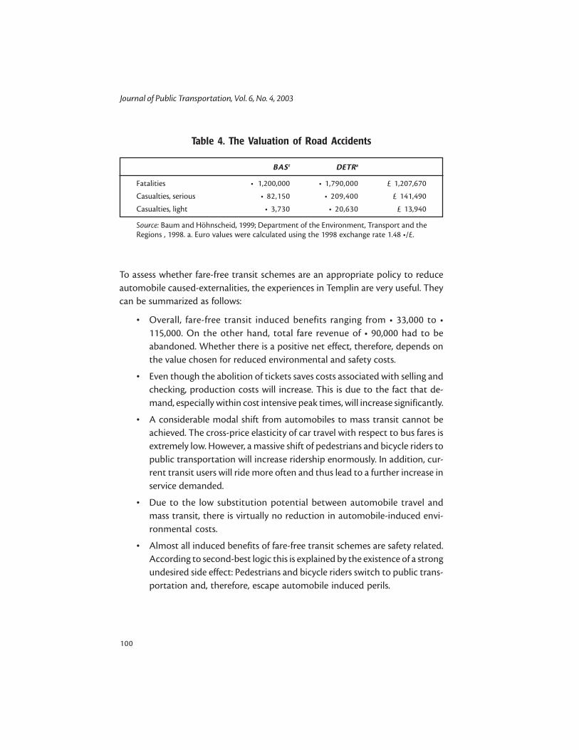
Journal of Public Transportation, Vol. 6, No. 4, 2003
100
Table 4. The Valuation of Road Accidents
To assess whether fare-free transit schemes are an appropriate policy to reduceautomobile caused-externalities, the experiences in Templin are very useful. Theycan be summarized as follows:
• Overall, fare-free transit induced benefits ranging from • 33,000 to •115,000. On the other hand, total fare revenue of • 90,000 had to beabandoned. Whether there is a positive net effect, therefore, depends onthe value chosen for reduced environmental and safety costs.
• Even though the abolition of tickets saves costs associated with selling andchecking, production costs will increase. This is due to the fact that de-mand, especially within cost intensive peak times, will increase significantly.
• A considerable modal shift from automobiles to mass transit cannot beachieved. The cross-price elasticity of car travel with respect to bus fares isextremely low. However, a massive shift of pedestrians and bicycle riders topublic transportation will increase ridership enormously. In addition, cur-rent transit users will ride more often and thus lead to a further increase inservice demanded.
• Due to the low substitution potential between automobile travel andmass transit, there is virtually no reduction in automobile-induced envi-ronmental costs.
• Almost all induced benefits of fare-free transit schemes are safety related.According to second-best logic this is explained by the existence of a strongundesired side effect: Pedestrians and bicycle riders switch to public trans-portation and, therefore, escape automobile induced perils.
BASt DETRa
Fatalities • 1,200,000 • 1,790,000 £ 1,207,670
Casualties, serious • 82,150 • 209,400 £ 141,490
Casualties, light • 3,730 • 20,630 £ 13,940
Source: Baum and Höhnscheid, 1999; Department of the Environment, Transport and theRegions , 1998. a. Euro values were calculated using the 1998 exchange rate 1.48 •/£.

Externalities by Automobiles and Fare-Free Transit in Germany
101
Conlcusion and AssessmentFollowing the extraordinary growth in automobile travel over the last few de-cades, transportation externalities have risen to an alarming level. Policies aimed atreducing external costs (e.g., accidents, noise, pollution) can be distinguished intotwo different approaches: the automobile burdening push policy and the transitfavoring pull policy. Against this background the introduction of general fare-freetransit schemes appears to experience a renaissance in several European cities; bestknown are the Belgian Hasselt and the German City of Templin. The staggeringincreases in ridership in both cities seem to be a clear indication of the overwhelm-ing success of this policy approach. In addition, a study carried out for the Ger-man Federal Ministry of Transportation found that the benefits of fare-free transitin Templin could offset the costs. According to the study, the positive net benefitshows that fare-free transit is a viable policy instrument to curb automobile causedexternalities. Is this the first step toward a paradigm shift in transportation andenvironmental policies?
Fare-free schemes are based on the economic theory of the second best. Underfirst-best conditions, service level and prices of transportation modes were opti-mized separately; the price should be equal to the respective marginal cost. How-ever, since the private marginal costs of automobile travel lie below the socialmarginal costs, a welfare improving second-best approach suggests a reduction oftransit fares below the first-best optimum. Under particular conditions, this evenallows to derive a fare of zero. The objective of this policy is to encourage automo-bile users to shift to environmentally friendly public transportation. An undesiredside effect of fare-free transit, however, may be an increase in the demand byformer transit users and the attraction of users of nonmotorized transportation.
This could be confirmed in the City of Templin. A study aimed at quantifying thebenefits of fare-free transit found that ridership increased by 1,200 percent. Thevast majority of this additional demand consisted of former transit users andattracted pedestrians and bicycle riders. The shift from automobile to transit wasonly minimal. Depending on the values chosen for intangibles, a positive net ben-efit may result. This is due mainly to a reduction in fatalities and casualties. Sincepedestrians and bicycle riders belong to the most endangered road users, everydecrease in these modes will necessarily lead to a reduction of automobile causedcosts. The undesired side effect thus becomes the main effect.

Journal of Public Transportation, Vol. 6, No. 4, 2003
102
This astounding result appears to be cynical. Should it be the goal of transporta-tion policies to minimize external automobile costs by converting nonmotorizedtravel into motorized travel? Using the same argument one could introduce a taxon pedestrians and bicycle riders as well. The effect would be more direct andmore efficient. In fact, this would be a paradigm shift. Overall, we can state thatautomobile-caused externalities should not be answered by transit fare reduc-tions. Externalities should better be countered at the source, by internalizing policyapproaches.
Endnotes1 For instance, the PDS is demanding fare-free transit for major German cities suchas Mainz (200,000 inhabitants) and Munich (1.2 million inhabitants).
2 This is equal to $4.1 billion in 2002 prices.
3 A comprehensive literature survey is provided by Small (1992).
4 In general, uncovered costs of accidents or infrastructure can lead to inefficientprices as well. Second-best analyses are to be found, e.g., in Calabresi (1970). Therelationship between road accidents and transit pricing was investigated by Allsopand Robertson (1994) and Evans and Morrison (1997). , S. 117 ff. For a compre-hensive approach encompassing infrastructure, congestion, environmental, safety,and distribution effects see De Borger et al. (1996).
5 Compare for instance, the discussion lead in the then German language journalKyklos by Bohley (1973) and Blankart (1975). Also, in English, Baum (1973).
6 Encompassing holiday hotel city center, private errands, and other trip purposes.
7 The following values per avoided automobile kilometer driven were assumed:noise • 0.030; CO, NOx, SO2, HC and particulate matter • 0.022; CO2 • 0.008.

Externalities by Automobiles and Fare-Free Transit in Germany
103
References
Allsop, R. E., and S. A. Robertson. 1994. Road casualties in relation to public trans-port policy. Journal of Transport Economics and Policy 28: 61–82.
Baum, H. 1973. Free public transport. Journal of Transport Economics and Policy 7:3–19.
Baum, H. and K. Höhnscheid. 1999. Volkswirtschaftliche Kosten derPersonenschäden im Straßenverkehr. Bericht der BASt, Reihe Mensch undSicherheit, Heft M 102. Bergisch-Gladbach, Germany: BASt.
Blankart, C. B. 1975. Der Nulltarif im Nahverkehr als kollektive und individuelleEntscheidung. Kyklos 28: 154–157.
Bohley, P. 1973. Der Nulltarif im Nahverkehr. Kyklos 26: 113–142.
Bös, D. 1986. Public enterprise economics. Theory and application. Amsterdam andNew York: North Holland.
Bundesministerium für Verkehr, Bau- und Wohnungswesen. 2000. Verkehr inZahlen 2000. Hamburg: Deutscher Verkehrs-Verlag.
Calabresi, G. 1970. The costs of accidents: a legal and economic analysis. New Ha-ven, CT: Yale University Press.
City of Hasselt. 2000. Mobility with an eye on the environment—Hasselt, an examplefor Europe. Hasselt, Belgium: City of Hasselt.
De Borger, B., I. Mayeres, S. Proost, and S. Wouters. 1996. Optimal pricing of urbanpassenger transport. Journal of Transport Economics and Policy 30: 31–54.
Department of the Environment, Transport and the Regions. 1998. HighwaysEconomics (Note 1). London: DETR.
Deutscher Bundestag, Unterrichtung durch die Bundesregierung, Bericht derBundesregierung 1996 über die Entwicklung der Kostenunterdeckung imöffentlichen Personennahverkehr (ÖPNV). Drucksache 13/7552 vom 22.04.97.Prior reports are to be found in Drs. 12/1965 (1992), Drs. 10/6773 (1987), Drs.9/1658 (1982), Drs. 7/4556 (1976). Bonn: Deutscher Bundestag.
Evans, A. W., and A. D. Morrison. 1997. Incorporating accident risk and disrup-tion in economic models of public transport. Journal of Transport Economicsand Policy 31: 117–146.

Journal of Public Transportation, Vol. 6, No. 4, 2003
104
Federal Transit Administration (FTA). 2002. National Transit Database. Online:http://www.fta.dot.gov/ntl/database.html. Washington, DC: FTA.
Glaister, S. 1974. Generalised consumer surplus and public transport pricing. TheEconomic Journal 84: 849–867.
Glaister, S. and D. Lewis. 1978. An integrated fares policy for transport in London.Journal of Public Economics 9: 341–355.
Gómez-Ibáñez, J.1999. Pricing. In Essays in transportation economics and policy. J.Gómez-Ibáñez, W. Tye, and C. Winston, eds. Washington DC: Brookings In-stitution Press, pp. 99–136.
Hodge, D. C. et al. 1994. Fare-free policy: costs, impacts on transit service, andattainment of transit system goals. Springfield, VA: Washington State Depart-ment of Transportation.
Jansson, J. O. 1980. Transport system optimization and pricing. Stockholm: Eco-nomic Research Institute at the Stockholm School of Economics.
Keuchel, S., et al. 2000. Kommunaler Nutzen von ÖPNV-Angeboten am Beispielfahrscheinfreier Tarif-/Finanzierungskonzepte bei Stadtbusverkehren vonKlein-und Mittelstädten. Forschungsbericht FE 70.588/99 im Auftrag desBundesministers für Verkehr, Bau-und Wohnungswesen. Recklinghausen,Germany: Fachhochschule Gelsenkirchen.
Lipsey, R. G., and K. Lancaster. 1956/57. The general theory of second best. Reviewof Economic Studies 26: 11–32.
Mohring, H. 1972. Optimization and scale economics in urban bus transporta-tion. The American Economic Review 62: 591–604.
Pucher, J., A. Markstedt, and I. Hirschman. 1983. Impacts of subsidies on the costsof urban public transport. Journal of Transport Economics and Policy 17: 155–176.
Ratzenberger, R. 1997. Finanzleistungen für den öffentlichen Personennahverkehr.ifo Schnelldienst Nr. 14/97, (Munich: ifo).
Small, K. 1992. Urban transportation economics. Chur, Switzerland: Harwood Aca-demic Publishers.
Stadt Templin. 2000. Fahrscheinfreier Stadtverkehr der Stadt Templin.Informationsschrift. Templin, Germany: Stadt Templin.

Externalities by Automobiles and Fare-Free Transit in Germany
105
Storchmann, K. 1999. Das Defizit im öffentlichen Personennahverkehr in Theorieund Empirie. (Schriftenreihe des Rheinisch-Westfälischen Instituts fürWirtschaftsforschung, Neue Folge 64. Berlin: Duncker & Humblodt.
Storchmann, K. 2001. The impact of fuel taxes on public transport—an empiricalassessment for Germany. Transport Policy 8: 19–28.
Turvey, R. 1971. Economic analysis and public enterprises. London: Allan & Unwin.
Turvey, R., and H. Mohring. 1975. Optimal bus fares. Journal of Transport Econom-ics and Policy 9: 280–286.
WIBERA Wirtschaftsberatung AG. 1996. Darstellung der Kosten, Erträge,Betriebsergebnisse und Leistungen des ÖPNV im Jahre 1993 und Vergleichmit vorangegangenen Zeiträumen, insbesondere 1988, getrennt nachBallungsräumen und übriges Bundesgebiet sowie alten und neuenBundesländern. Schlußbericht. Untersuchung im Auftrag des Bundesministersfür Verkehr, FE-Nr. 70456/94. Düsseldorf, Germany: Wibera.
About the Author
KARL STORCHMANN ([email protected]) is a lecturer in the Econom-ics Department at Yale University. His main research interests are appliedmicroeconomic issues related to environmental and resource economics, trans-portation, energy, and agriculture. His most recent articles have appeared in Trans-port Policy and Agricultural Economics.

Journal of Public Transportation, Vol. 6, No. 4, 2003
108