Volume and Complexity Bounded Simplification of SolidModel Represented by Binary Space Partition

Pu Huang Charlie C. L. Wang∗

Department of Mechanical and Automation EngineeringThe Chinese University of Hong Kong

Shatin, N.T., Hong Kong, Chinacwang@mae.cuhk.edu.hk

ABSTRACTWe present a volume and complexity bounded solid sim-plification of models represented by Binary Space Partition

(BSP). Depending on the compact and robust representa-tion of a solid model in BSP-tree, the boundary surface of asimplified model is guaranteed to be two-manifold and self-intersection free. Two techniques are investigated in thispaper. The volume bounded convex simplification can col-lapse parts with small volumes on the model into a simpleconvex volume enclosing the volumetric cells on the inputmodel. The selection of which region to simplify is basedon a volume-difference metric, with the help of which thevolume difference between the given model and the simpli-fied one is minimized. Another technique is a plane collapsemethod which reduces the depth of the BSP-tree while stillpreserving volume bounding. These two techniques are in-tegrated into our solid simplification algorithm to give sat-isfactory results. Related applications are given at the endof this paper to demonstrate the function of our algorithm.

Categories and Subject DescriptorsI.3.5 [Computational Geometry and Object Model-ing]: Boundary representations – Curve, surface, solid, andobject representations

KeywordsSimplification, Volume Bounded, Complexity Bounded, Bi-nary Space Partition, Solid Model

1. INTRODUCTIONBinary Space Partition (BSP) tree is a binary tree whichrepresents a d-space partitioning by hyper-planes for dimen-sion d, and it can provide an exact representation of arbi-trary polyhedral objects in d-dimensional space. A balancedBSP representation of a model allows fast point classifica-tion [5,20], collision detection [13,17], visible surface detec-tion [9] and Boolean operations [4, 20, 25]. It also generates

∗Corresponding Author.

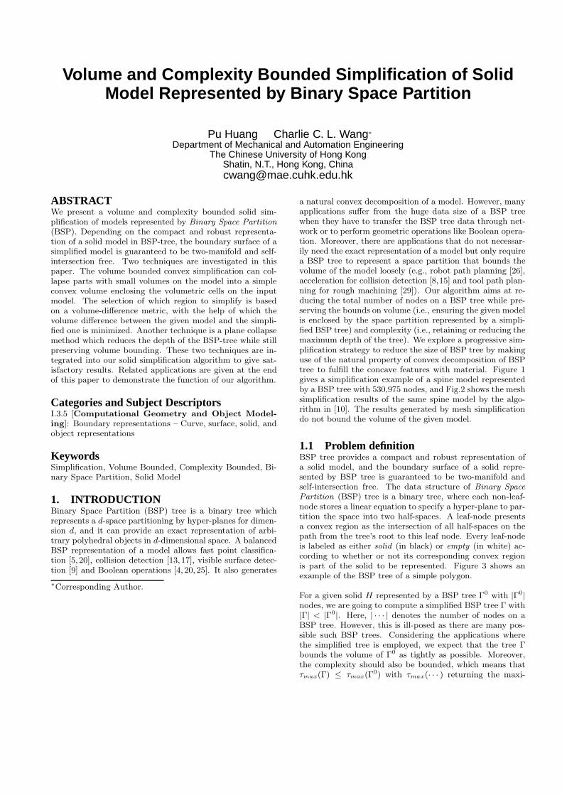
a natural convex decomposition of a model. However, manyapplications suffer from the huge data size of a BSP treewhen they have to transfer the BSP tree data through net-work or to perform geometric operations like Boolean opera-tion. Moreover, there are applications that do not necessar-ily need the exact representation of a model but only requirea BSP tree to represent a space partition that bounds thevolume of the model loosely (e.g., robot path planning [26],acceleration for collision detection [8,15] and tool path plan-ning for rough machining [29]). Our algorithm aims at re-ducing the total number of nodes on a BSP tree while pre-serving the bounds on volume (i.e., ensuring the given modelis enclosed by the space partition represented by a simpli-fied BSP tree) and complexity (i.e., retaining or reducing themaximum depth of the tree). We explore a progressive sim-plification strategy to reduce the size of BSP tree by makinguse of the natural property of convex decomposition of BSPtree to fulfill the concave features with material. Figure 1gives a simplification example of a spine model representedby a BSP tree with 530,975 nodes, and Fig.2 shows the meshsimplification results of the same spine model by the algo-rithm in [10]. The results generated by mesh simplificationdo not bound the volume of the given model.

1.1 Problem definitionBSP tree provides a compact and robust representation ofa solid model, and the boundary surface of a solid repre-sented by BSP tree is guaranteed to be two-manifold andself-intersection free. The data structure of Binary Space

Partition (BSP) tree is a binary tree, where each non-leaf-node stores a linear equation to specify a hyper-plane to par-tition the space into two half-spaces. A leaf-node presentsa convex region as the intersection of all half-spaces on thepath from the tree’s root to this leaf node. Every leaf-nodeis labeled as either solid (in black) or empty (in white) ac-cording to whether or not its corresponding convex regionis part of the solid to be represented. Figure 3 shows anexample of the BSP tree of a simple polygon.

For a given solid H represented by a BSP tree Γ0 with |Γ0|nodes, we are going to compute a simplified BSP tree Γ with|Γ| < |Γ0|. Here, | · · · | denotes the number of nodes on aBSP tree. However, this is ill-posed as there are many pos-sible such BSP trees. Considering the applications wherethe simplified tree is employed, we expect that the tree Γbounds the volume of Γ0 as tightly as possible. Moreover,the complexity should also be bounded, which means thatτmax(Γ) ≤ τmax(Γ0) with τmax(· · · ) returning the maxi-

Figure 1: The solid simplification of a spine model. From the left: the input spine solid (with 530k nodes ona BSP tree and the maximum depth, τmax, of the tree is 124), a slightly simplified solid (with 70% of nodesretained and τmax = 112), a simplified solid (with 30% of nodes and τmax = 113), a further simplified solid (with5% of nodes and τmax = 114), and a coarser solid (with only 0.5% of nodes and τmax = 114) – regions in differentconvex hulls are displayed in different colors. The relative volume errors of the simplified solids are 1.83%,23.5%, 77.9% and 148.2% of the original model respectively.

Figure 2: The mesh simplification results of thespine model using the quadric error metrics in [10]:(left) about 5% of vertices are retained, and (right)only 0.5% of vertices of the original model are re-tained. The simplified models do not bound thevolume of the original spine.

mum depth of a tree. The tightness of volume bounding ismeasured by the volume difference between the solids rep-resented by the simplified and the original trees as

M(Γ) = |V (Γ) − V (Γ0)|, (1)

where V (Γ) =∑

siV (si) is evaluated by summing up the

volumes of all solid leaf-nodes si ∈ Γ.

1.2 Related workWe briefly review the work closely related to the conversionbetween B-rep and BSP tree, the volume simplification, BSPtree based solid modeling and other applications.

At present, the most popular representation for free-formobjects is piecewise linear B-rep – polygonal meshes, whichis convenient for local manipulation and rendering. How-ever, it inherits the common drawback of B-rep – difficultfor space evaluation (e.g., point membership classificationand volume computation). The most conventional methodto convert polyhedra from B-rep to BSP tree is the approach

Figure 3: A polygon can be decomposed to be rep-resented by a BSP tree, where non-leaf-nodes are ingrey and leaf-nodes are in black or white accordingto whether its convex region is solid or empty.

presented by Thibault and Naylor in [25]. The algorithm isbased on repeatedly selecting a planar polygon on the sur-face of a given model as a clipping plane (i.e., the non-leaf-node on BSP tree) to separate other polygons into its leftand right half-spaces. Although the constructed BSP treecan present the boundary surface of a given model exactly,the tree itself is not well balanced. Bajaj et al. introduced aprogressive conversion from B-rep to BSP tree for streaminggeometric modeling in [1]. They used eigen decompositionof the Euler tensor which represents surface inertia to cutthe model in order to get relatively balanced BSP tree. Forthe BSP trees constructed by different strategies, the simpli-fied solids generated by our method are quite different (seethe illustration shown in Fig.4). In our tests, the simplifiedmodels obtained from a balanced BSP tree by [1] generallygive better visual appearance than the results of the BSP

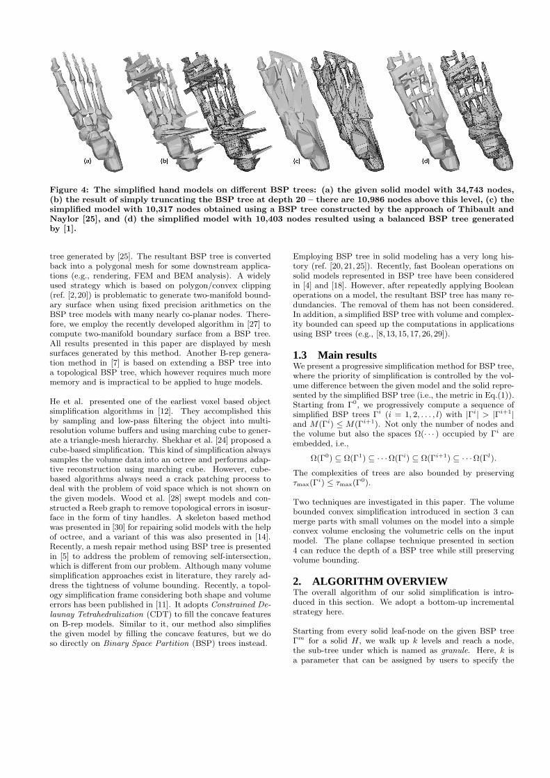
Figure 4: The simplified hand models on different BSP trees: (a) the given solid model with 34,743 nodes,(b) the result of simply truncating the BSP tree at depth 20 – there are 10,986 nodes above this level, (c) thesimplified model with 10,317 nodes obtained using a BSP tree constructed by the approach of Thibault andNaylor [25], and (d) the simplified model with 10,403 nodes resulted using a balanced BSP tree generatedby [1].

tree generated by [25]. The resultant BSP tree is convertedback into a polygonal mesh for some downstream applica-tions (e.g., rendering, FEM and BEM analysis). A widelyused strategy which is based on polygon/convex clipping(ref. [2,20]) is problematic to generate two-manifold bound-ary surface when using fixed precision arithmetics on theBSP tree models with many nearly co-planar nodes. There-fore, we employ the recently developed algorithm in [27] tocompute two-manifold boundary surface from a BSP tree.All results presented in this paper are displayed by meshsurfaces generated by this method. Another B-rep genera-tion method in [7] is based on extending a BSP tree intoa topological BSP tree, which however requires much morememory and is impractical to be applied to huge models.

He et al. presented one of the earliest voxel based objectsimplification algorithms in [12]. They accomplished thisby sampling and low-pass filtering the object into multi-resolution volume buffers and using marching cube to gener-ate a triangle-mesh hierarchy. Shekhar et al. [24] proposed acube-based simplification. This kind of simplification alwayssamples the volume data into an octree and performs adap-tive reconstruction using marching cube. However, cube-based algorithms always need a crack patching process todeal with the problem of void space which is not shown onthe given models. Wood et al. [28] swept models and con-structed a Reeb graph to remove topological errors in isosur-face in the form of tiny handles. A skeleton based methodwas presented in [30] for repairing solid models with the helpof octree, and a variant of this was also presented in [14].Recently, a mesh repair method using BSP tree is presentedin [5] to address the problem of removing self-intersection,which is different from our problem. Although many volumesimplification approaches exist in literature, they rarely ad-dress the tightness of volume bounding. Recently, a topol-ogy simplification frame considering both shape and volumeerrors has been published in [11]. It adopts Constrained De-

launay Tetrahedralization (CDT) to fill the concave featureson B-rep models. Similar to it, our method also simplifiesthe given model by filling the concave features, but we doso directly on Binary Space Partition (BSP) trees instead.

Employing BSP tree in solid modeling has a very long his-tory (ref. [20, 21, 25]). Recently, fast Boolean operations onsolid models represented in BSP tree have been consideredin [4] and [18]. However, after repeatedly applying Booleanoperations on a model, the resultant BSP tree has many re-dundancies. The removal of them has not been considered.In addition, a simplified BSP tree with volume and complex-ity bounded can speed up the computations in applicationsusing BSP trees (e.g., [8, 13,15,17,26,29]).

1.3 Main resultsWe present a progressive simplification method for BSP tree,where the priority of simplification is controlled by the vol-ume difference between the given model and the solid repre-sented by the simplified BSP tree (i.e., the metric in Eq.(1)).Starting from Γ0, we progressively compute a sequence ofsimplified BSP trees Γi (i = 1, 2, . . . , l) with |Γi| > |Γi+1|and M(Γi) ≤ M(Γi+1). Not only the number of nodes andthe volume but also the spaces Ω(· · · ) occupied by Γi areembedded, i.e.,

Ω(Γ0) ⊆ Ω(Γ1) ⊆ · · ·Ω(Γi) ⊆ Ω(Γi+1) ⊆ · · ·Ω(Γl).

The complexities of trees are also bounded by preservingτmax(Γ

i) ≤ τmax(Γ0).

Two techniques are investigated in this paper. The volumebounded convex simplification introduced in section 3 canmerge parts with small volumes on the model into a simpleconvex volume enclosing the volumetric cells on the inputmodel. The plane collapse technique presented in section4 can reduce the depth of a BSP tree while still preservingvolume bounding.

2. ALGORITHM OVERVIEWThe overall algorithm of our solid simplification is intro-duced in this section. We adopt a bottom-up incrementalstrategy here.

Starting from every solid leaf-node on the given BSP treeΓm for a solid H , we walk up k levels and reach a node,the sub-tree under which is named as granule. Here, k isa parameter that can be assigned by users to specify the

granularity of simplification in each step; k = 6 is selectedin all our examples in this paper. We wish to approximatethe solid inside a granule γ by a simplified BSP sub-tree cγ

that holds fewer nodes (i.e., half-spaces). Also, the depth ofcγ should satisfy τmax(cγ) ≤ τmax(γ). Details about how toobtain cγ are presented in sections 3 and 4.

When replacing γ by the half-spaces in cγ , the volume erroradded to the new tree is (V (cγ) − V (γ)). Therefore, in ouralgorithm, all candidate granules are inserted into a prior-ity queue keyed by this volume error, which can guaranteethat the granule with the minimal volume error is alwayssimplified first. After a simplification step, a new granule isidentified and inserted into the queue.

The simplification procedure keeps running until the volumedifference M(Γn) of the current new tree Γn or the reducednumber of nodes exceeds the given thresholds. The tree Γ isthen reported as the simplification result. The pseudo-codeis presented in Algorithm BSPSolidSimplification.

Algorithm 1 BSPSolidSimplification

1: Verr = 0 and nred = 0;2: Duplicate a BSP tree Γ from the input Γ0;3: Initialize the priority queue Θ;4: Find all granules starting from the left deepest solid leaf-

nodes; We visit the tree in the LMR order5: for all granules γ do6: Compute the simplified BSP sub-tree cγ ;7: Insert γ into Θ by the weight (V (cγ) − V (γ));8: end for9: while Θ 6= φ do

10: Remove the granule γcur from the top of Θ;11: On the BSP tree Γ, replace γcur by cγcur ;12: Verr = Verr + (V (cγcur ) − V (γcur));13: nred = nred + ∆γcur ;

∆γcur reporting the number of nodes reduced14: Update the queue Θ by adding the new granule;

Note that the new granule is determined by the new

solid leaf-node on γcur15: if (Verr > threshold) OR (nred > threshold) then16: break;17: end if18: end while19: return Γn;

3. VOLUME BOUNDED CONVEX SIMPLI-FICATION

The method for computing a volume bounded simplificationfrom a given BSP tree Γm is presented in this section. For agiven granule represented by a BSP sub-tree γ, we wish toapproximate the solid inside it by a simplified BSP tree withfewer nodes (i.e., half-spaces). A BSP tree representationprovides a natural convex decomposition for a model. Thenumber of solid convex hulls equals to the number of blacknodes. For example in Fig.3, the granule of node B containstwo convex hulls, where the one below D is surrounded byA+, B+, C− and D−, and the one below E is formed byA+, B− and E−. Here the signs specify the portion of theircorresponding half-spaces.

Proposition 1 For a set of convex hulls ci ∈ ℜ3, if the

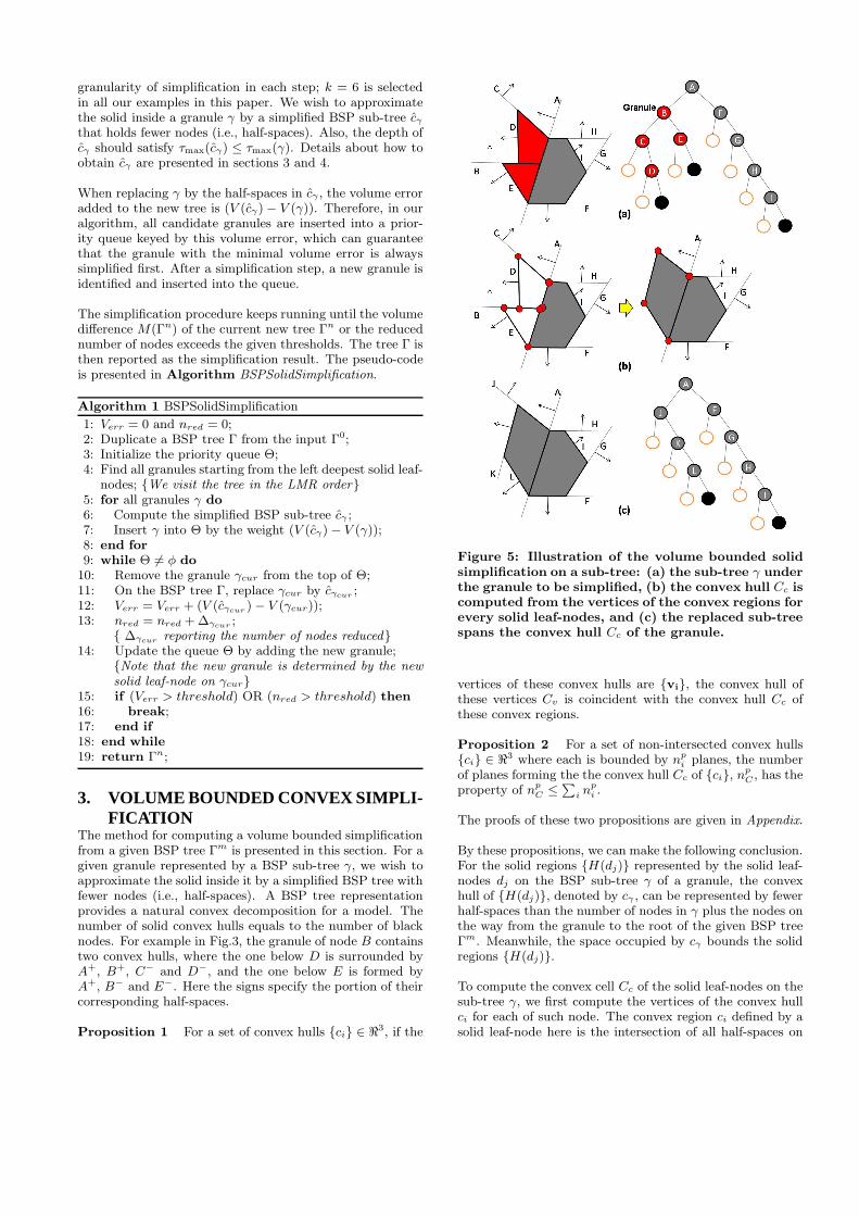
Figure 5: Illustration of the volume bounded solidsimplification on a sub-tree: (a) the sub-tree γ underthe granule to be simplified, (b) the convex hull Cc iscomputed from the vertices of the convex regions forevery solid leaf-nodes, and (c) the replaced sub-treespans the convex hull Cc of the granule.

vertices of these convex hulls are vi, the convex hull ofthese vertices Cv is coincident with the convex hull Cc ofthese convex regions.

Proposition 2 For a set of non-intersected convex hullsci ∈ ℜ3 where each is bounded by n

pi planes, the number

of planes forming the the convex hull Cc of ci, npC , has the

property of npC ≤

∑in

pi .

The proofs of these two propositions are given in Appendix.

By these propositions, we can make the following conclusion.For the solid regions H(dj) represented by the solid leaf-nodes dj on the BSP sub-tree γ of a granule, the convexhull of H(dj), denoted by cγ , can be represented by fewerhalf-spaces than the number of nodes in γ plus the nodes onthe way from the granule to the root of the given BSP treeΓm. Meanwhile, the space occupied by cγ bounds the solidregions H(dj).

To compute the convex cell Cc of the solid leaf-nodes on thesub-tree γ, we first compute the vertices of the convex hullci for each of such node. The convex region ci defined by asolid leaf-node here is the intersection of all half-spaces on

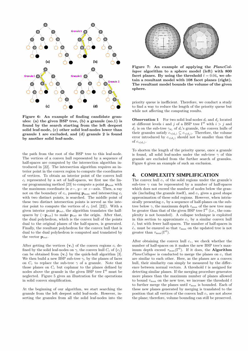
Figure 6: An example of finding candidate gran-ules: (a) the given BSP tree, (b) a granule (no.1) isfound by the search starting from the left deepestsolid leaf-node, (c) other solid leaf-nodes lower thangranule 1 are excluded, and (d) granule 2 is foundby another solid leaf-node.

the path from the root of the BSP tree to this leaf-node.The vertices of a convex hull represented by a sequence ofhalf-spaces are computed by the intersection algorithm in-troduced in [22]. The intersection algorithm requires an in-terior point in the convex region to compute the coordinatesof vertices. To obtain an interior point of the convex hullci represented by a set of half-spaces, we first use the lin-ear programming method [23] to compute a point pmax withthe maximum coordinate in x−, y− or z−axis. Then, a raynot on the boundary of ci, passing pmax and intersecting ci

with two distinct points, is searched. The middle point ofthese two distinct intersection points is served as the inte-rior point to compute the vertices of ci (ref. [22]). With agiven interior point pint, the algorithm translates the half-spaces by (−pint) to make pint as the origin. After that,the dual polyhedron, which is the convex hull of the pointsdual to the original planes of the half-spaces, is generated.Finally, the resultant polyhedron for the convex hull that isdual to the dual polyhedron is computed and translated bythe vector pint.

After getting the vertices vi of the convex regions ci de-fined by the solid leaf-nodes on γ, the convex hull Cc of cican be obtained from vi by the quick-hull algorithm [3].We then build a new BSP sub-tree γc by the planes of faceson Cc to replace the sub-tree γ of a granule. Note thatthose planes on Cc but coplanar to the planes defined bynodes above the granule in the given BSP tree Γ0 must beneglected. Figure 5 gives an illustration for the operationsin solid convex simplification.

At the beginning of our algorithm, we start searching thegranule from the left deepest solid leaf-node. However, in-serting the granules from all the solid leaf-nodes into the

Figure 7: An example of applying the PlaneCol-

lapse algorithm to a sphere model (left) with 800facet planes. By using the threshold t = 0.04, we ob-tain a resultant model with 108 facet planes (right).The resultant model bounds the volume of the givensphere.

priority queue is inefficient. Therefore, we conduct a studyto find a way to reduce the length of the priority queue butwhile not affecting the computing results.

Observation 1 For two solid leaf-nodes di and dj locatedat different levels i and j of a BSP tree Γ0 with i > j anddj is on the sub-tree γdi

of di’s granule, the convex hulls oftheir granules satisfy cγ(di) ⊆ cγ(dj ). Therefore, the volumeerror introduced by cγ(dj) should not be smaller than thatof cγ(di).

To shorten the length of the priority queue, once a granuleis found, all solid leaf-nodes under the sub-tree γ of thisgranule are excluded from the further search of granules.Figure 6 gives an example of such an exclusion.

4. COMPLEXITY SIMPLIFICATIONThe convex hull cγ of the solid regions under the granule’ssub-tree γ can be represented by a number of half-spaceswhich does not exceed the number of nodes below the gran-ule (including the granule itself), and cγ gives a good shapeapproximation of these solid regions. However, when intrin-sically presenting cγ by a sequence of half-planes on the sub-tree below γ, the maximum depth τmax of the new tree maybe greater than that of the given BSP tree Γ0 (i.e., the com-plexity is not bounded). A collapse technique is exploitedin this section to approximate cγ by a similar convex hullcγ but with fewer half-spaces. The number of half-spaces incγ must be ensured so that τmax on the updated tree is notgreater than τmax(Γ

0).

After obtaining the convex hull cγ , we check whether thenumber of half-spaces on it makes the new BSP tree’s max-imum depth exceed τmax(Γ

0). If it does, the AlgorithmPlaneCollapse is conducted to merge the planes on cγ thatare similar to each other. Here, as the planes are a convexhull, their similarity can simply be measured by the differ-ence between normal vectors. A threshold t is assigned fordetecting similar planes. If the merging procedure generatesmore planes than the maximum number of planes allowedto bound τmax on the new tree, we increase the threshold tto further merge the planes until τmax is bounded. Each ofthese new planes generated by merging is translated to theposition that all vertices of the convex hull cγ are not abovethe plane; therefore, volume bounding can still be preserved.

More than that, only the planes which do not belong to thenodes above the granule on the BSP tree Γm are processedby the collapse algorithm to be merged. Pseudo-code of Al-gorithm PlaneCollapse is listed below. Figure 7 shows theresult of applying this algorithm to a sphere.

Algorithm 2 PlaneCollapse

Require: the threshold t, the list of planes to be collapsedLI , and the convex hull cγ

Ensure: the output list of planes LO

1: while LI is NOT empty do2: Randomly remove a plane from LI ;3: Insert into Lt;4: for all ∈ LI do5: if the normals have ‖n − n‖

2 < t then6: Remove from LI and insert it into Lt;7: end if8: end for9: Calculate the average normal navg of all planes in Lt;

10: Clear up Lt;11: Find a vertex v ∈ cγ that maximizes (v · navg);12: Determine a new plane new by navg and v;13: Insert new into LO;14: end while15: return LO ;

5. RESULTSWe have already implemented the proposed algorithm ina C++ program. The examples shown in this paper are alltested on a PC with Intel Core 2 Quad CPU Q6600 2.4GHz.

5.1 Experimental tests and discussionThe results of experimental tests on our algorithm are en-couraging. The first example is a spine model with morethan 530k nodes on a BSP tree, which is shown in Fig.1. Oursolid simplification algorithm can significantly reduce thenumber of nodes on the BSP tree. The original spine modelis guaranteed to be enclosed by the simplified solids, and themaximum depth of the simplified BSP tree is bounded bythe maximum depth of the given tree.

The second example is a chair model in Fig.8. Together withthe bump model shown in Fig.9, we study the performanceof our solid simplification algorithm with and without theplane collapse step. An interesting result we observed isthat, when stopping with a similar number of retained nodes,the simplification procedure without the plane collapse stepfills up more void spaces. This is because more nodes arereduced after consolidating a granule if the plane collapsestep is taken. Therefore, when reaching a similar number ofreduced nodes, fewer granules are consolidated, which meansthat less void volume is filled if the plane collapse step istaken. However, the shape of convex hull cγ without takingthe plane collapse bounds the shape of the given model moretightly than cγ , the one with fewer nodes on the sub-tree.

Two more examples from biomedical applications are shownin Fig.10 and 11. The computational statistics of our algo-rithm are listed in Table 1. It shows that our algorithm isvery fast when being applied to models with a moderate size.The thresholds chosen in the Algorithm BSPSolidSimplifi-

cation are specified by users according to their applications.

Table 1: Computational Statistics

Given BSP Tree Resultant BSP Tree*Model Fig. Nodes τmax Nodes τmax Time

Spine 1 530,975 124 3,787 114 7.31 min.Chair 8 247,979 140 3,331 129 2.27 min.Bump 9 202,621 308 4,293 301 2.25 min.Donna 10 1,520,949 188 6,831 163 39.7 min.

Hand 11 38,535 46 723 43 12.5 sec.Twirl 14 23,461 35 481 31 5.38 sec.Venus 15 11,673 79 389 43 3.28 sec.

*Note that we report the full simplification with both thevolume and the complexity bounded.

Figure 10: The simplification results of the donnamodel (the BSP tree has 1,520,949 nodes and τmax =188) obtained by retaining different numbers ofnodes.

Choosing thresholds with very few nodes and very large al-lowed volume error eventually makes the results of our al-gorithm converge to a loose convex hull1 of the given model(see Fig.12). Our algorithm proposed in this paper can beemployed in many applications. Several are demonstratedbelow.

5.2 Application I: post-processing for Booleanoperation

The first application is the post-processing of the BSP treegenerated by repeatedly applying Boolean operations to amodel. For the BSP tree obtained in such a scenario, thereare lots of redundancies retained. For example, the modelshown in Fig.13 is produced by simulating shaping opera-tion (using Boolean operation) on a piece of stock material.Although the shape of the resultant model is simple, its cor-responding BSP tree generated by the approach in [18] con-tains 787,683 nodes. To remove the redundancy, we applyour solid simplification approach to this BSP tree with anextremely small volume threshold (e.g., 10−8). The number

1When neglecting the plane collapse step, the algorithm con-verges to the tight convex hull.

Figure 8: A simplification example of a chair model: (top row) the results obtained from full solid simplifica-tion algorithm, and (bottom row) the complexity simplification is neglected. Simplification stops at differentnumbers of retained nodes compared with the given BSP tree: (a) 50%, (b) 30%, (c) 10%, (d) 5% and (e) 1.5%.

Figure 9: A simplification example of a bump model: (top row) the results obtained from full solid simplifica-tion algorithm, and (bottom row) the complexity simplification is neglected. Simplification stops at differentnumbers of retained nodes compared with the given BSP tree: (a) 70%, (b) 50%, (c) 30%, (d) 10% and (e) 5%.

of nodes on the tree can be reduced from 787,683 to 410,575in 9.953 seconds.

5.3 Application II: collision detectionThe BSP tree representation of solid models has been em-ployed to accelerate collision detection in many applications(ref. [8,15]). A common strategy to speed up collision detec-tion algorithm is to develop some methods to fast excludethose collision-free cases, while not missing any of those pos-sibly collided cases. Meanwhile, there are also some appli-cations, where physical simulation involving collision detec-tion is only conducted on a coarser level of geometry than theshape in visual rendering (e.g., games). Our solid simplifica-tion algorithm presented in this paper satisfies the require-ments of a coarse collision detection. First, the simplifiedBSP tree with fewer nodes can be adopted to detect thosecollision-free cases efficiently. Second, our simplification re-sults tightly bound the volume of the given models, which

guarantees that the collided cases will never be missed. Inaddition, the tight volume bounding could also have morecollision-free cases being quickly detected. Moreover, as thecomplexity of the simplified BSP tree is also bounded, thesimplified BSP tree usually gives better speed performance.See the examples of simplified models shown in Fig.14 and15.

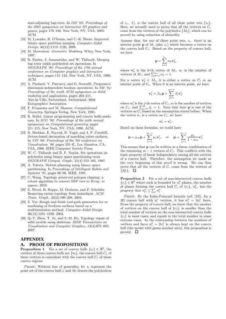
5.4 Application III: rough material prepara-tion

The last application demonstrated in this paper is the gener-ation of rough material prepared for further subtractive ma-chining. In product manufacturing, the final part can onlybe produced by subtractive machining; thus, the rough ma-terial prepared should bound the volume of the final product– our method can ensure this. Although the convex hull ofthe designed part can always satisfy this requirement, itsshape may have a large volume difference compared with

Figure 11: The results of simplifying the hand model(the BSP tree has 38,535 nodes and τmax = 46) to theBSP trees with different percentages of nodes on thegiven model.

Figure 12: The result of our simplification algorithmconverges to a loose convex hull of the given model.

the designed model, which leads to a long machining time.Therefore, some coarser shapes which still bound the givenmodel is wanted (e.g., the model with volume simplified asshown in Fig.16). A more practical strategy for solving thisproblem may be the feature-based approach like [16]; how-ever, our algorithm provides a general geometric tool forimplementing feature-based methods.

6. CONCLUSIONS AND DISCUSSIONIn this paper, we present a general solid simplification al-gorithm that works on solids represented by Binary Space

Partition (BSP) trees. The volume and the complexity ofgiven models are bounded in our simplification algorithm.Depending on the compact and robust representation ofa solid model in BSP-tree, boundary surfaces of the sim-plified models are guaranteed to be two-manifold and self-intersection free. Two techniques have been investigated inthis paper. The volume bounded convex simplification cancollapse parts with small volumes on the model into a simpleconvex volume enclosing the volumetric cells on the input

Figure 13: The results of repeatedly applyingBoolean operations to a box model. The redun-dancy on the resultant BSP tree can be removedby our solid simplification algorithm.

Figure 14: The twirl model (with 23,461 nodes onthe BSP tree and τmax = 35) has been simplified intosolids represented by BSP trees with different num-bers of nodes compared with the given BSP tree.The convex hull contains 69 half-spaces. The resul-tant BSP trees form several convex hulls which aredisplayed in different colors. The maximum depthsof the simplified BSP trees are: 28, 28, 28, 31 and35 respectively.

model. The selection of which region to simplify is basedon a volume-difference metric, which minimizes the volumedifference between the given model and the simplified oneis minimized. The plane collapse approach can reduce thedepth of a BSP tree while still preserving volume bounding.The effectiveness of our approach has been proved by severalexperimental tests.

Two problems of the current approach need to be solvedin our future research. First, the plane collapse approachsomewhat loose the tightness of volume bound. A zero vol-ume error approach is planned to be developed from a com-binatorial algorithm. Another alternative is to adopt theLloyd algorithm based shape approximation like [6]. Sec-ond, the shape of a simplified solid does depend on the waythe BSP tree is constructed (see the illustration in Fig.4).We plan to develop some feature-based approach to con-struct BSP trees for applications like feature-based multi-

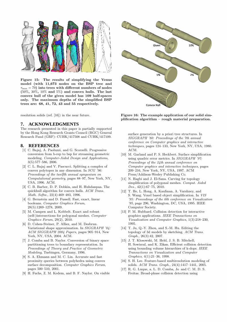
Figure 15: The results of simplifying the Venusmodel (with 11,673 nodes on the BSP tree andτmax = 79) into trees with different numbers of nodes(50%, 30%, 10% and 5%) and convex hulls. The lastconvex hull of the given model has 109 half-spacesonly. The maximum depths of the simplified BSPtrees are: 68, 41, 72, 43 and 55 respectively.

resolution solids (ref. [16]) in the near future.

7. ACKNOWLEDGMENTSThe research presented in this paper is partially supportedby the Hong Kong Research Grants Council (RGC) GeneralResearch Fund (GRF): CUHK/417508 and CUHK/417109.

8. REFERENCES[1] C. Bajaj, A. Paoluzzi, and G. Scorzelli. Progressive

conversion from b-rep to bsp for streaming geometricmodeling. Computer-Aided Design and Applications,3(5):577–586, 2006.

[2] C. L. Bajaj and V. Pascucci. Splitting a complex ofconvex polytopes in any dimension. In SCG ’96:

Proceedings of the twelfth annual symposium on

Computational geometry, pages 88–97, New York, NY,USA, 1996. ACM.

[3] C. B. Barber, D. P. Dobkin, and H. Huhdanpaa. Thequickhull algorithm for convex hulls. ACM Trans.

Math. Softw., 22(4):469–483, 1996.

[4] G. Bernstein and D. Fussell. Fast, exact, linearbooleans. Computer Graphics Forum,28(5):1269–1278, 2009.

[5] M. Campen and L. Kobbelt. Exact and robust(self-)intersections for polygonal meshes. Computer

Graphics Forum, 29(2), 2010.

[6] D. Cohen-Steiner, P. Alliez, and M. Desbrun.Variational shape approximation. In SIGGRAPH ’04:

ACM SIGGRAPH 2004 Papers, pages 905–914, NewYork, NY, USA, 2004. ACM.

[7] J. Comba and B. Naylor. Conversion of binary spacepartitioning trees to boundary representation. InProceedings of Theory and Practice of Geometric

Modeling, Tuebingen, Germany, 1996.

[8] S. A. Ehmann and M. C. Lin. Accurate and fastproximity queries between polyhedra using convexsurface decomposition. Computer Graphics Forum,pages 500–510, 2001.

[9] H. Fuchs, Z. M. Kedem, and B. F. Naylor. On visible

Figure 16: The example application of our solid sim-plification algorithm – rough material preparation.

surface generation by a priori tree structures. InSIGGRAPH ’80: Proceedings of the 7th annual

conference on Computer graphics and interactive

techniques, pages 124–133, New York, NY, USA, 1980.ACM.

[10] M. Garland and P. S. Heckbert. Surface simplificationusing quadric error metrics. In SIGGRAPH ’97:

Proceedings of the 24th annual conference on

Computer graphics and interactive techniques, pages209–216, New York, NY, USA, 1997. ACMPress/Addison-Wesley Publishing Co.

[11] N. Hagbi and J. El-Sana. Carving for topologysimplification of polygonal meshes. Comput. Aided

Des., 42(1):67–75, 2010.

[12] T. He, L. Hong, A. Kaufman, A. Varshney, andS. Wang. Voxel based object simplification. In VIS

’95: Proceedings of the 6th conference on Visualization

’95, page 296, Washington, DC, USA, 1995. IEEEComputer Society.

[13] P. M. Hubbard. Collision detection for interactivegraphics applications. IEEE Transactions on

Visualization and Computer Graphics, 1(3):218–230,1995.

[14] T. Ju, Q.-Y. Zhou, and S.-M. Hu. Editing thetopology of 3d models by sketching. ACM Trans.

Graph., 26(3):42, 2007.

[15] J. T. Klosowski, M. Held, J. S. B. Mitchell,H. Sowizral, and K. Zikan. Efficient collision detectionusing bounding volume hierarchies of k-dops. IEEE

Transactions on Visualization and Computer

Graphics, 4(1):21–36, 1998.

[16] S. H. Lee. Feature-based multiresolution modeling ofsolids. ACM Trans. Graph., 24(4):1417–1441, 2005.

[17] R. G. Luque, a. L. D. Comba, Jo and C. M. D. S.Freitas. Broad-phase collision detection using

semi-adjusting bsp-trees. In I3D ’05: Proceedings of

the 2005 symposium on Interactive 3D graphics and

games, pages 179–186, New York, NY, USA, 2005.ACM.

[18] M. Lysenko, R. D’Souza, and C.-K. Shene. Improvedbinary space partition merging. Computer-Aided

Design, 40(12):1113–1120, 2008.

[19] M. Mortenson. Geometric Modeling. Wiley, New York,1997.

[20] B. Naylor, J. Amanatides, and W. Thibault. Mergingbsp trees yields polyhedral set operations. InSIGGRAPH ’90: Proceedings of the 17th annual

conference on Computer graphics and interactive

techniques, pages 115–124, New York, NY, USA, 1990.ACM.

[21] A. Paoluzzi, V. Pascucci, and G. Scorzelli. Progressivedimension-independent boolean operations. In SM ’04:

Proceedings of the ninth ACM symposium on Solid

modeling and applications, pages 203–211,Aire-la-Ville, Switzerland, Switzerland, 2004.Eurographics Association.

[22] F. Preparata and M. Shamos. Computational

Geometry. Springer-Verlag, New York, 1985.

[23] R. Seidel. Linear programming and convex hulls madeeasy. In SCG ’90: Proceedings of the sixth annual

symposium on Computational geometry, pages211–215, New York, NY, USA, 1990. ACM.

[24] R. Shekhar, E. Fayyad, R. Yagel, and J. F. Cornhill.Octree-based decimation of marching cubes surfaces.In VIS ’96: Proceedings of the 7th conference on

Visualization ’96, pages 335–ff., Los Alamitos, CA,USA, 1996. IEEE Computer Society Press.

[25] W. C. Thibault and B. F. Naylor. Set operations onpolyhedra using binary space partitioning trees.SIGGRAPH Comput. Graph., 21(4):153–162, 1987.

[26] A. Tokuta. Motion planning using binary spacepartitioning. In Proceedings of Intelligent Robots and

Systems ’91, pages 86–90. IEEE, 1991.

[27] C. Wang. Topology preserved polygon clipping: arobust algorithm to convert BSP tree to B-rep. to

appear, 2010.

[28] Z. Wood, H. Hoppe, M. Desbrun, and P. Schroder.Removing excess topology from isosurfaces. ACM

Trans. Graph., 23(2):190–208, 2004.

[29] Z. Yin. Rough and finish tool-path generation for ncmachining of freeform surfaces based on amultiresolution method. Computer-Aided Design,36(12):1231–1239, 2004.

[30] Q.-Y. Zhou, T. Ju, and S.-M. Hu. Topology repair ofsolid models using skeletons. IEEE Transactions on

Visualization and Computer Graphics, 13(4):675–685,2007.

APPENDIXA. PROOF OF PROPOSITIONSProposition 1 For a set of convex hulls ci ∈ ℜ3, thevertices of these convex hulls are vi, the convex hull Cv ofthese vertices is coincident with the convex hull Cc of theseconvex regions.

Proof. Without loss of generality, let si represent thepoint set of the convex hull ci and Mi denote the polyhedron

of ci. Cc is the convex hull of all these point sets si.Here, we actually need to prove that all the vertices on Cc

come from the vertices of the polyhedra Mi, which can beproved by using reduction of absurdity.

Assume that, for one of these point sets, sr, there is aninterior point p of Mr (also sr) which becomes a vertex onthe convex hull Cc. Based on the property of convex hull,we have

p =

nr∑

k=1

αkvrk,

where vrk is the k-th vertex of Mr, nr is the number of

vertices of Mr, and∑nr

k=1 αk = 1.

For a vertex vrk ∈ Mr, it is either a vertex on Cc or an

interior point of Cc. When it is an interior point, we have

vrk = βmp +

m−1∑

j=1

βjvcj ,

where vcj is the j-th vertex of Cc, m is the number of vertices

on Cc, and∑m

j=1 βj = 1. Note that here p is one of thevertices on Cc based on the assumption stated before. Whenthe vertex vr is a vertex on Cc, we have

vrk = vc

j .

Based on these formulas, we could have

p = µmp +m−1∑

j=1

µjvcj , ⇒ p =

m−1∑

j=1

µj

1 − µm

vcj .

This means that p can be written as a linear combination ofthe remaining m − 1 vertices of Cc. This conflicts with thebasic property of linear independency among all the verticesof a convex hull. Therefore, the assumption we made atthe very beginning of this proof is wrong. We can thusprove that all the vertices of Cc come from the vertices ofMi.

Proposition 2 For a set of non-intersected convex hullsci ∈ ℜ3 where each is bounded by n

pi planes, the number

of planes forming the convex hull Cc of ci, npC , has the

property that npC ≤

∑in

pi .

Proof. By the Euler-Poincare formula (ref. [19]), for a3D convex hull with nv

i vertices, it has npi = 2nv

i faces.From the property of convex hull, we know that the numberof vertices on the convex hull of ci, is smaller than thetotal number of vertices on the non-intersected convex hullsci in most cases, and equals to the total number in someextreme cases. As the relationship between the numbers ofvertices and faces n

pi = 2nv

i is always kept on the convexhull (the model with genus number zero), this proposition isproved.