Embed Size (px)
Citation preview
Volume Imbalance and Algorithmic Trading
Alvaro [email protected]
University College Londonjoint work with
Ryan Donnelly, EPFLSebastian Jaimungal, University of Toronto
December, 2014
1 / 59
Outline
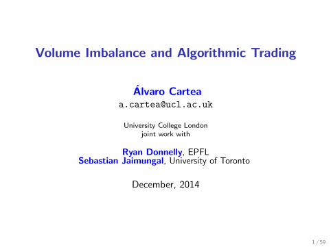
I The limit order book.
I Volume order imbalance as an indicator of market behaviour.
I Imbalance model and market model.
I Optimal trading problem.
I The value of knowing imbalance.
2 / 59

The Limit Order BookI The limit order book is a record of collective interest to buy or
sell certain quantities of an asset at a certain price.
Buy Orders Sell OrdersPrice Volume Price Volume60.00 80 60.10 7559.90 100 60.20 7559.80 90 60.30 50
I Graphical representation of the limit order book:
Price
Volum
e
3 / 59
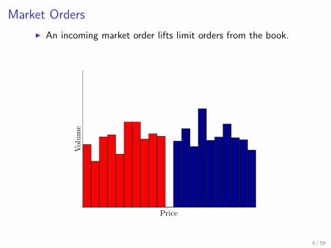
Market Orders
I An incoming market order lifts limit orders from the book.
Price
Volume
4 / 59
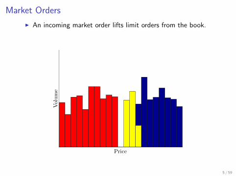
Market Orders
I An incoming market order lifts limit orders from the book.
Price
Volume
5 / 59
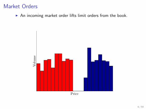
Market Orders
I An incoming market order lifts limit orders from the book.
Price
Volume
6 / 59
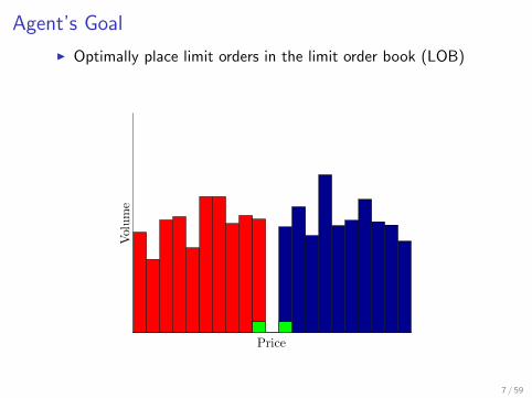
Agent’s Goal
I Optimally place limit orders in the limit order book (LOB)
Price
Volume
7 / 59
Agent’s Goal
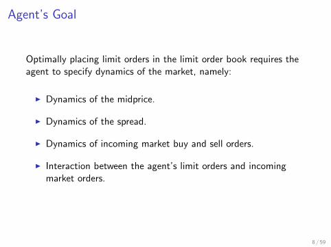
Optimally placing limit orders in the limit order book requires theagent to specify dynamics of the market, namely:
I Dynamics of the midprice.
I Dynamics of the spread.
I Dynamics of incoming market buy and sell orders.
I Interaction between the agent’s limit orders and incomingmarket orders.
8 / 59
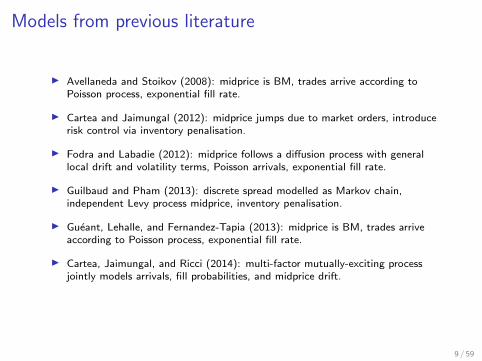
Models from previous literature
I Avellaneda and Stoikov (2008): midprice is BM, trades arrive according toPoisson process, exponential fill rate.
I Cartea and Jaimungal (2012): midprice jumps due to market orders, introducerisk control via inventory penalisation.
I Fodra and Labadie (2012): midprice follows a diffusion process with generallocal drift and volatility terms, Poisson arrivals, exponential fill rate.
I Guilbaud and Pham (2013): discrete spread modelled as Markov chain,independent Levy process midprice, inventory penalisation.
I Gueant, Lehalle, and Fernandez-Tapia (2013): midprice is BM, trades arriveaccording to Poisson process, exponential fill rate.
I Cartea, Jaimungal, and Ricci (2014): multi-factor mutually-exciting processjointly models arrivals, fill probabilities, and midprice drift.
9 / 59
Volume Order Imbalance
10 / 59
Volume Order Imbalance
I Volume order imbalance is the proportion of best interest onthe bid side.
I Defined as:
It =V bt
V bt + V a
t
.
I V bt is the volume at the best bid at time t.
I V at is the volume at the best ask at time t.
I It ∈ [0, 1].
11 / 59
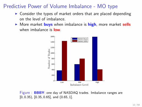
Predictive Power of Volume Imbalance - MO typeI Consider the types of market orders that are placed depending
on the level of imbalance.I More market buys when imbalance is high, more market sells
when imbalance is low.
Low Mid High0
200
400
600
800
1000
1200
1400
1600
Imbalance Level
Number
ofTrades
Market BuysMarket Sells
Figure : BBBY: one day of NASDAQ trades. Imbalance ranges are[0, 0.35), [0.35, 0.65], and (0.65, 1].
12 / 59
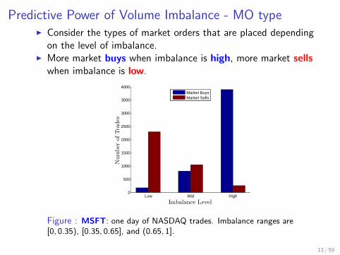
Predictive Power of Volume Imbalance - MO typeI Consider the types of market orders that are placed depending
on the level of imbalance.I More market buys when imbalance is high, more market sells
when imbalance is low.
Low Mid High0
500
1000
1500
2000
2500
3000
3500
4000
Imbalance Level
Number
ofTrades
Market BuysMarket Sells
Figure : MSFT: one day of NASDAQ trades. Imbalance ranges are[0, 0.35), [0.35, 0.65], and (0.65, 1].
13 / 59
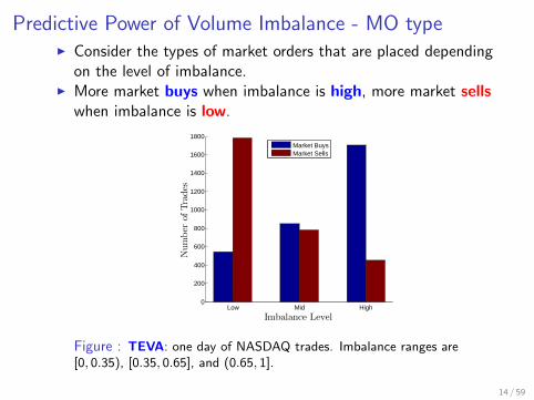
Predictive Power of Volume Imbalance - MO typeI Consider the types of market orders that are placed depending
on the level of imbalance.I More market buys when imbalance is high, more market sells
when imbalance is low.
Low Mid High0
200
400
600
800
1000
1200
1400
1600
1800
Imbalance Level
Number
ofTrades
Market BuysMarket Sells
Figure : TEVA: one day of NASDAQ trades. Imbalance ranges are[0, 0.35), [0.35, 0.65], and (0.65, 1].
14 / 59
Volume Imbalance and Midprice Change
15 / 59
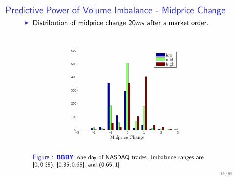
Predictive Power of Volume Imbalance - Midprice ChangeI Distribution of midprice change 20ms after a market order.
−3 −2 −1 0 1 2 30
100
200
300
400
500
600
Midprice Change
lowmidhigh
Figure : BBBY: one day of NASDAQ trades. Imbalance ranges are[0, 0.35), [0.35, 0.65], and (0.65, 1].
16 / 59

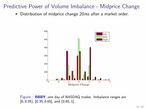
Predictive Power of Volume Imbalance - Midprice ChangeI Distribution of midprice change 20ms after a market order.
−3 −2 −1 0 1 2 30
100
200
300
400
500
600
Midprice Change
lowmidhigh
Figure : BBBY: one day of NASDAQ trades. Imbalance ranges are[0, 0.35), [0.35, 0.65], and (0.65, 1].
17 / 59
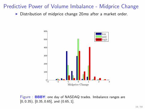
Predictive Power of Volume Imbalance - Midprice ChangeI Distribution of midprice change 20ms after a market order.
−3 −2 −1 0 1 2 30
100
200
300
400
500
600
Midprice Change
lowmidhigh
Figure : BBBY: one day of NASDAQ trades. Imbalance ranges are[0, 0.35), [0.35, 0.65], and (0.65, 1].
18 / 59
Predictive Power of Volume Imbalance - Midprice ChangeI Distribution of midprice change 20ms after a market order.
−3 −2 −1 0 1 2 30
100
200
300
400
500
600
Midprice Change
lowmidhigh
Figure : BBBY: one day of NASDAQ trades. Imbalance ranges are[0, 0.35), [0.35, 0.65], and (0.65, 1].
19 / 59
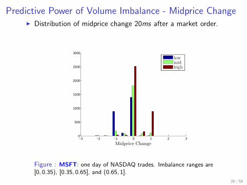
Predictive Power of Volume Imbalance - Midprice ChangeI Distribution of midprice change 20ms after a market order.
−3 −2 −1 0 1 2 30
500
1000
1500
2000
2500
3000
Midprice Change
lowmidhigh
Figure : MSFT: one day of NASDAQ trades. Imbalance ranges are[0, 0.35), [0.35, 0.65], and (0.65, 1].
20 / 59
Predictive Power of Volume Imbalance - Midprice ChangeI Distribution of midprice change 20ms after a market order.
−3 −2 −1 0 1 2 30
500
1000
1500
2000
2500
3000
Midprice Change
lowmidhigh
Figure : MSFT: one day of NASDAQ trades. Imbalance ranges are[0, 0.35), [0.35, 0.65], and (0.65, 1].
21 / 59
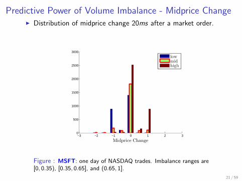
Predictive Power of Volume Imbalance - Midprice ChangeI Distribution of midprice change 20ms after a market order.
−3 −2 −1 0 1 2 30
500
1000
1500
2000
2500
3000
Midprice Change
lowmidhigh
Figure : MSFT: one day of NASDAQ trades. Imbalance ranges are[0, 0.35), [0.35, 0.65], and (0.65, 1].
22 / 59
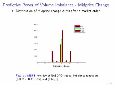
Predictive Power of Volume Imbalance - Midprice ChangeI Distribution of midprice change 20ms after a market order.
−3 −2 −1 0 1 2 30
500
1000
1500
2000
2500
3000
Midprice Change
lowmidhigh
Figure : MSFT: one day of NASDAQ trades. Imbalance ranges are[0, 0.35), [0.35, 0.65], and (0.65, 1].
23 / 59
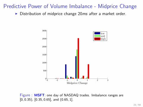
Predictive Power of Volume Imbalance - Midprice ChangeI Distribution of midprice change 20ms after a market order.
−3 −2 −1 0 1 2 30
100
200
300
400
500
600
700
800
Midprice Change
lowmidhigh
Figure : TEVA: one day of NASDAQ trades. Imbalance ranges are[0, 0.35), [0.35, 0.65], and (0.65, 1].
24 / 59
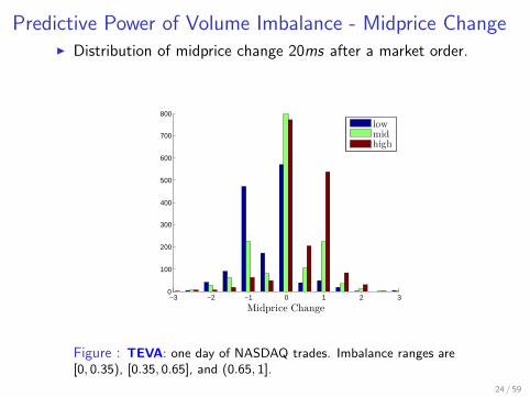
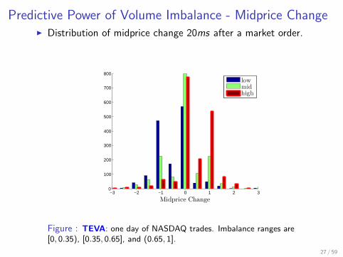
Predictive Power of Volume Imbalance - Midprice ChangeI Distribution of midprice change 20ms after a market order.
−3 −2 −1 0 1 2 30
100
200
300
400
500
600
700
800
Midprice Change
lowmidhigh
Figure : TEVA: one day of NASDAQ trades. Imbalance ranges are[0, 0.35), [0.35, 0.65], and (0.65, 1].
25 / 59
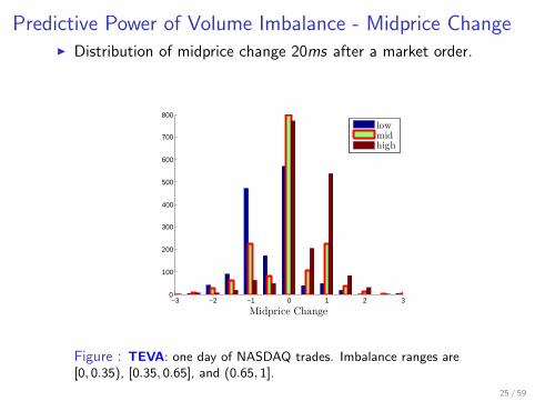
Predictive Power of Volume Imbalance - Midprice ChangeI Distribution of midprice change 20ms after a market order.
−3 −2 −1 0 1 2 30
100
200
300
400
500
600
700
800
Midprice Change
lowmidhigh
Figure : TEVA: one day of NASDAQ trades. Imbalance ranges are[0, 0.35), [0.35, 0.65], and (0.65, 1].
26 / 59
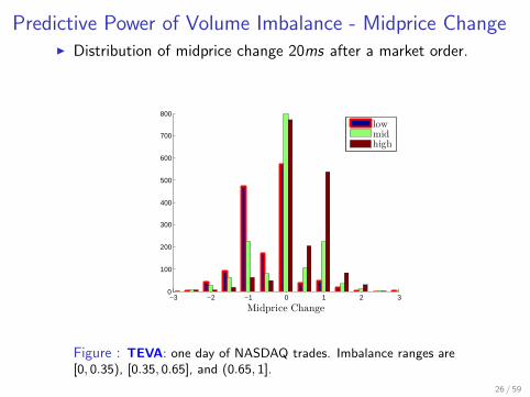
Predictive Power of Volume Imbalance - Midprice ChangeI Distribution of midprice change 20ms after a market order.
−3 −2 −1 0 1 2 30
100
200
300
400
500
600
700
800
Midprice Change
lowmidhigh
Figure : TEVA: one day of NASDAQ trades. Imbalance ranges are[0, 0.35), [0.35, 0.65], and (0.65, 1].
27 / 59

Where to post in the LOB?
28 / 59

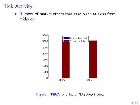
Tick ActivityI Number of market orders that take place at ticks from
midprice.
Buys Sells0
500
1000
1500
2000
2500
3000
Beyond first tick
Within first tick
Figure : BBBY: one day of NASDAQ trades.
29 / 59
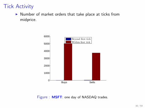
Tick ActivityI Number of market orders that take place at ticks from
midprice.
Buys Sells0
1000
2000
3000
4000
5000
6000
Beyond first tick
Within first tick
Figure : MSFT: one day of NASDAQ trades.
30 / 59
Tick ActivityI Number of market orders that take place at ticks from
midprice.
Buys Sells0
500
1000
1500
2000
2500
3000
3500
Beyond first tick
Within first tick
Figure : TEVA: one day of NASDAQ trades.
31 / 59
Market Model
32 / 59
Market Model
I Rather than model imbalance directly, a finite state imbalanceregime process is considered, Zt ∈ {1, . . . , nZ}.
I Zt will act as an approximation to the true value of imbalance.
I The interval [0, 1] is subdivided in to nZ subintervals. Zt = kcorresponds to It lying within the k th subinterval.
I The spread ∆t also takes values in a finite state space,∆t ∈ {1, . . . , n∆}.
33 / 59
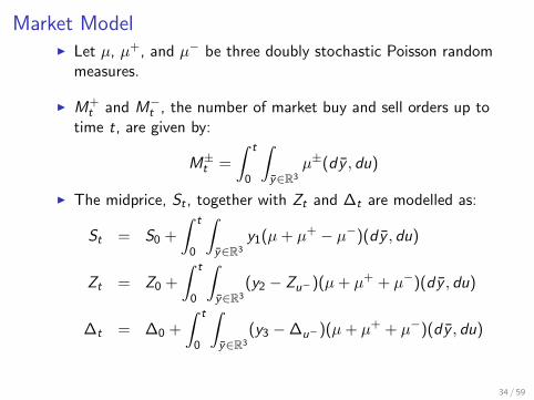
Market ModelI Let µ, µ+, and µ− be three doubly stochastic Poisson random
measures.
I M+t and M−t , the number of market buy and sell orders up to
time t, are given by:
M±t =
∫ t
0
∫y∈R3
µ±(dy , du)
I The midprice, St , together with Zt and ∆t are modelled as:
St = S0 +
∫ t
0
∫y∈R3
y1(µ+ µ+ − µ−)(dy , du)
Zt = Z0 +
∫ t
0
∫y∈R3
(y2 − Zu−)(µ+ µ+ + µ−)(dy , du)
∆t = ∆0 +
∫ t
0
∫y∈R3
(y3 −∆u−)(µ+ µ+ + µ−)(dy , du)
34 / 59
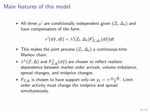
Main features of this model
I All three µi are conditionally independent given (Zt ,∆t) andhave compensators of the form:
ν i (dy , dt) = λi (Zt ,∆t)FiZt ,∆t
(dy)dt
I This makes the joint process (Zt ,∆t) a continuous-timeMarkov chain.
I λ±(Z ,∆) and F±Z ,∆(dy) are chosen to reflect realisticdependence between market order arrivals, volume imbalance,spread changes, and midprice changes.
I FZ ,∆ is chosen to have support only on y1 = ± y3−∆2 . Limit
order activity must change the midprice and spreadsimultaneously.
35 / 59
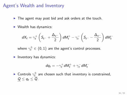
Agent’s Wealth and Inventory
I The agent may post bid and ask orders at the touch.
I Wealth has dynamics:
dXt = γ+t
(St− +
∆t−
2
)dM+
t − γ−t(St− −
∆t−
2
)dM−t
where γ±t ∈ {0, 1} are the agent’s control processes.
I Inventory has dynamics:
dqt = −γ+t dM
+t + γ−t dM
−t
I Controls γ±t are chosen such that inventory is constrained,Q ≤ qt ≤ Q.
36 / 59
Optimal Trading
37 / 59
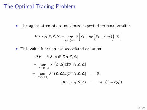
The Optimal Trading Problem
I The agent attempts to maximize expected terminal wealth:
H(t, x , q, S,Z ,∆) = sup(γ±t )∈A
E[XT + qT
(ST − `(qT )
)∣∣∣∣Ft
]
I This value function has associated equation:
∂tH + λ(Z ,∆)E[DH|Z ,∆]
+ supγ+∈{0,1}
λ+(Z ,∆)E[D+H|Z ,∆]
+ supγ−∈{0,1}
λ−(Z ,∆)E[D−H|Z ,∆] = 0 ,
H(T , x , q, S ,Z) = x + q(S − `(q)) .
38 / 59
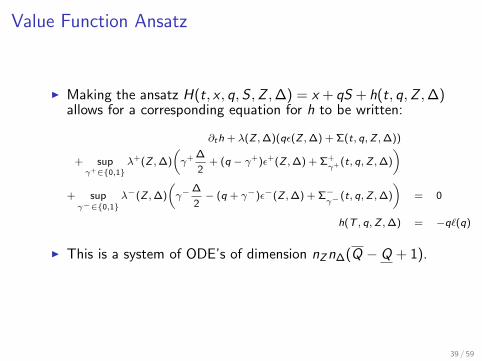
Value Function Ansatz
I Making the ansatz H(t, x , q,S ,Z ,∆) = x + qS + h(t, q,Z ,∆)allows for a corresponding equation for h to be written:
∂th + λ(Z ,∆)(qε(Z ,∆) + Σ(t, q,Z ,∆))
+ supγ+∈{0,1}
λ+(Z ,∆)
(γ+ ∆
2+ (q − γ+)ε+(Z ,∆) + Σ+
γ+ (t, q,Z ,∆)
)+ supγ−∈{0,1}
λ−(Z ,∆)
(γ−
∆
2− (q + γ−)ε−(Z ,∆) + Σ−
γ−(t, q,Z ,∆)
)= 0
h(T , q,Z ,∆) = −q`(q)
I This is a system of ODE’s of dimension nZn∆(Q − Q + 1).
39 / 59
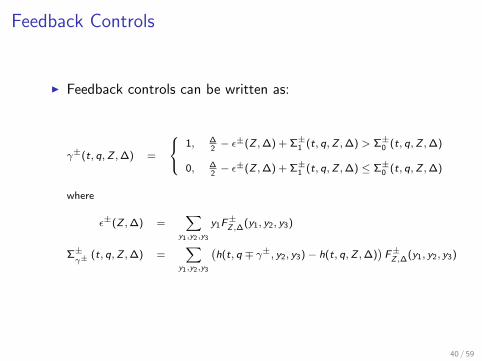
Feedback Controls
I Feedback controls can be written as:
γ±(t, q,Z ,∆) =
1, ∆2− ε±(Z ,∆) + Σ±1 (t, q,Z ,∆) > Σ±0 (t, q,Z ,∆)
0, ∆2− ε±(Z ,∆) + Σ±1 (t, q,Z ,∆) ≤ Σ±0 (t, q,Z ,∆)
where
ε±(Z ,∆) =∑
y1,y2,y3
y1F±Z ,∆(y1, y2, y3)
Σ±γ±
(t, q,Z ,∆) =∑
y1,y2,y3
(h(t, q ∓ γ±, y2, y3)− h(t, q,Z ,∆)
)F±Z ,∆(y1, y2, y3)
40 / 59
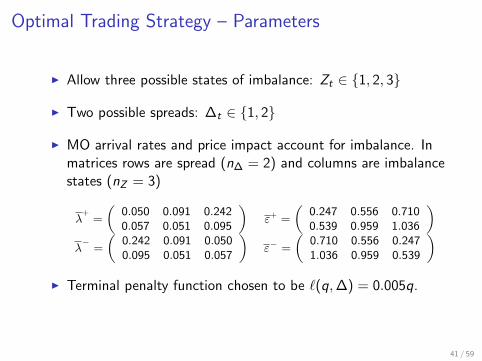
Optimal Trading Strategy – Parameters
I Allow three possible states of imbalance: Zt ∈ {1, 2, 3}
I Two possible spreads: ∆t ∈ {1, 2}
I MO arrival rates and price impact account for imbalance. Inmatrices rows are spread (n∆ = 2) and columns are imbalancestates (nZ = 3)
λ+
=
(0.050 0.091 0.2420.057 0.051 0.095
)ε+ =
(0.247 0.556 0.7100.539 0.959 1.036
)λ−
=
(0.242 0.091 0.0500.095 0.051 0.057
)ε− =
(0.710 0.556 0.2471.036 0.959 0.539
)I Terminal penalty function chosen to be `(q,∆) = 0.005q.
41 / 59
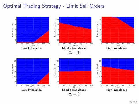
Optimal Trading Strategy - Limit Sell Orders
0 100 200 300 400 500 600
−20
−10
0
10
20
Time
Inventory
Level
Low Imbalance
0 100 200 300 400 500 600
−20
−10
0
10
20
Time
Inventory
Level
Middle Imbalance
0 100 200 300 400 500 600
−20
−10
0
10
20
Time
Inventory
Level
High Imbalance
∆ = 1
0 100 200 300 400 500 600
−20
−10
0
10
20
Time
Inventory
Level
Low Imbalance
0 100 200 300 400 500 600
−20
−10
0
10
20
Time
Inventory
Level
Middle Imbalance
0 100 200 300 400 500 600
−20
−10
0
10
20
Time
Inventory
Level
High Imbalance
∆ = 2
42 / 59
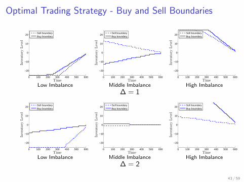
Optimal Trading Strategy - Buy and Sell Boundaries
0 100 200 300 400 500 600
−20
−10
0
10
20
Time
Inventory
Level
Sell boundaryBuy boundary
Low Imbalance
0 100 200 300 400 500 600
−20
−10
0
10
20
Time
Inventory
Level
Sell boundaryBuy boundary
Middle Imbalance
0 100 200 300 400 500 600
−20
−10
0
10
20
Time
Inventory
Level
Sell boundaryBuy boundary
High Imbalance
∆ = 1
0 100 200 300 400 500 600
−20
−10
0
10
20
Time
Inventory
Level
Sell boundaryBuy boundary
Low Imbalance
0 100 200 300 400 500 600
−20
−10
0
10
20
Time
Inventory
Level
Sell boundaryBuy boundary
Middle Imbalance
0 100 200 300 400 500 600
−20
−10
0
10
20
Time
Inventory
Level
Sell boundaryBuy boundary
High Imbalance
∆ = 2
43 / 59
The Value of Knowing Imbalance
44 / 59
The Value of Knowing Imbalance
I The number of imbalance regimes is an important modellingchoice.
I A large number of regimes can begin to cause observation andparameter estimation problems.
I A small number of regimes will not benefit as much from thepredictive information.
I How does the performance of an agent depend on the numberimbalance regimes in the model?
45 / 59
Simulation Procedure
I One day of data is simulated according to the model withnZ = 8.
I These data are used to estimate parameters of the modelwhen nZ = 1, 2, 4, and 8 by collapsing observable imbalancestates together.
I The “optimal” strategy is computed for each of these fourchoices of nZ .
I Ten minutes of data are simulated according to the originalmodel (nZ = 8), and each trading strategy’s performance istested against it (plus two additional “naive” strategies).
I The previous step is repeated 50,000 times to get adistribution of performance results.
46 / 59
Simulation Results
−1 −0.8 −0.6 −0.4 −0.2 0 0.2 0.4 0.60
0.5
1
1.5
2
2.5x 10
4
Terminal Wealth
Frequency
nZ = 8
nZ = 4
nZ = 2nZ = 1
naive
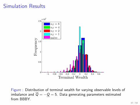
Figure : Distribution of terminal wealth for varying observable levels ofimbalance and Q = −Q = 5. Data generating parameters estimatedfrom BBBY.
47 / 59
Simulation Results
0 0.1 0.2 0.3 0.4 0.5−0.08
−0.06
−0.04
−0.02
0
0.02
0.04
0.06
Standard Deviation
Expectation
nZ = 8
nZ = 4
nZ = 2nZ = 1
naive 1naive 2
increasing Q
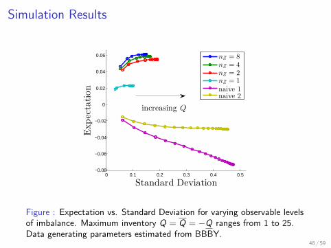
Figure : Expectation vs. Standard Deviation for varying observable levelsof imbalance. Maximum inventory Q = Q = −Q ranges from 1 to 25.Data generating parameters estimated from BBBY.
48 / 59
Simulation Results
−1 −0.8 −0.6 −0.4 −0.2 0 0.2 0.4 0.6 0.80
2000
4000
6000
8000
10000
12000
14000
Terminal Wealth
Frequency
nZ = 8
nZ = 4
nZ = 2nZ = 1
naive
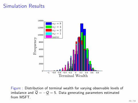
Figure : Distribution of terminal wealth for varying observable levels ofimbalance and Q = −Q = 5. Data generating parameters estimatedfrom MSFT.
49 / 59
Simulation Results
0 0.2 0.4 0.6 0.8 10
0.05
0.1
0.15
0.2
0.25
Standard Deviation
Expectation
nZ = 8
nZ = 4
nZ = 2nZ = 1
naive 1naive 2
increasing Q
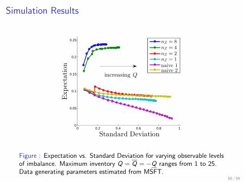
Figure : Expectation vs. Standard Deviation for varying observable levelsof imbalance. Maximum inventory Q = Q = −Q ranges from 1 to 25.Data generating parameters estimated from MSFT.
50 / 59
Simulation Results
−1 −0.5 0 0.5 10
2000
4000
6000
8000
10000
12000
Terminal Wealth
Frequency
nZ = 8
nZ = 4
nZ = 2nZ = 1
naive
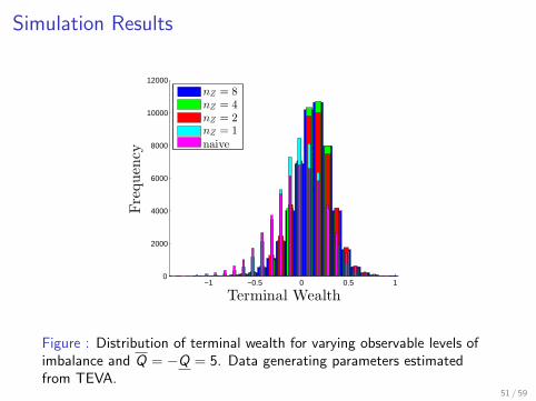
Figure : Distribution of terminal wealth for varying observable levels ofimbalance and Q = −Q = 5. Data generating parameters estimatedfrom TEVA.
51 / 59
Simulation Results
0 0.1 0.2 0.3 0.4 0.5 0.6 0.7 0.8
−0.1
−0.05
0
0.05
0.1
Standard Deviation
Expectation
nZ = 8
nZ = 4
nZ = 2nZ = 1
naive 1naive 2
increasing Q
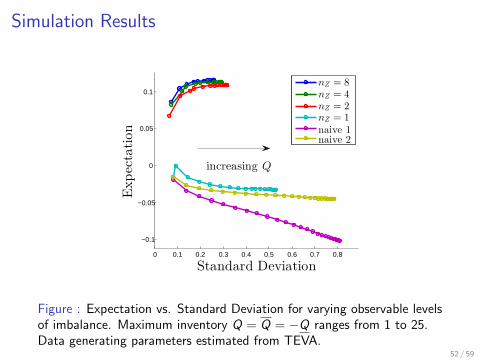
Figure : Expectation vs. Standard Deviation for varying observable levelsof imbalance. Maximum inventory Q = Q = −Q ranges from 1 to 25.Data generating parameters estimated from TEVA.
52 / 59
Conclusions
I The willingness of an agent to post limit orders is stronglydependent on the value of imbalance.
I Agent’s should post buy orders more aggressively and sellorders more conservatively when imbalance is high. Thisreflects taking advantage of short term speculation andprotecting against adverse selection.
I Corresponding opposite behaviour applies when imbalance islow.
I The additional value of being able to more accurately observeimbalance appears to have diminishing returns, but initiallythe additional value is very steep.
53 / 59

Future Endeavours
I Backtest strategies on real data.
I Investigate the effects of latency with respect to observingimbalance and spread.
I Expand the agent’s controls to allow multiple limit orderpostings at different prices and of different volumes.
I Incorporate more realistic interactions between market ordersand the agent’s limit orders (i.e. queueing priority and partialfills).
54 / 59
−0.02 0 0.02 0.040
500
1000
1500
2000
2500
Midprice Change−0.02 0 0.02 0.04
0
1000
2000
3000
4000
5000
6000
Midprice Change−0.02 0 0.02 0.04
0
1000
2000
3000
4000
5000
6000
Midprice Change
−0.02 0 0.02 0.040
1000
2000
3000
4000
5000
6000
7000
8000
Midprice Change−0.02 0 0.02 0.04
0
0.5
1
1.5
2
2.5
3x 10
4
Midprice Change−0.02 0 0.02 0.04
0
2000
4000
6000
8000
10000
12000
Midprice Change
−0.02 0 0.02 0.040
2000
4000
6000
8000
10000
Midprice Change−0.02 0 0.02 0.04
0
0.5
1
1.5
2
2.5
3
3.5x 10
4
Midprice Change−0.02 0 0.02 0.04
0
2000
4000
6000
8000
10000
12000
Midprice Change
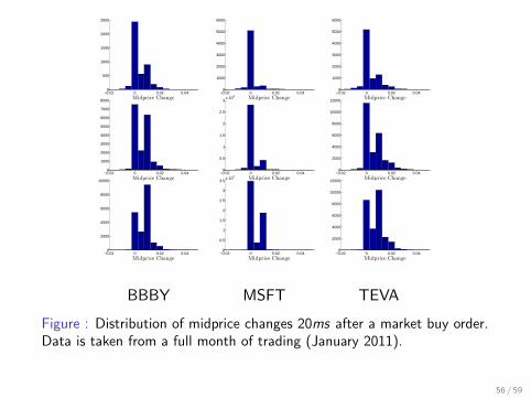
BBBY MSFT TEVA
Figure : Distribution of midprice changes 20ms after a market buy order.Data is taken from a full month of trading (January 2011).
56 / 59
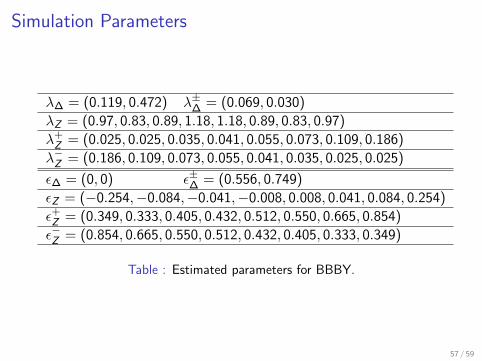
Simulation Parameters
λ∆ = (0.119, 0.472) λ±∆ = (0.069, 0.030)
λZ = (0.97, 0.83, 0.89, 1.18, 1.18, 0.89, 0.83, 0.97)
λ+Z = (0.025, 0.025, 0.035, 0.041, 0.055, 0.073, 0.109, 0.186)
λ−Z = (0.186, 0.109, 0.073, 0.055, 0.041, 0.035, 0.025, 0.025)
ε∆ = (0, 0) ε±∆ = (0.556, 0.749)
εZ = (−0.254,−0.084,−0.041,−0.008, 0.008, 0.041, 0.084, 0.254)
ε+Z = (0.349, 0.333, 0.405, 0.432, 0.512, 0.550, 0.665, 0.854)
ε−Z = (0.854, 0.665, 0.550, 0.512, 0.432, 0.405, 0.333, 0.349)
Table : Estimated parameters for BBBY.
57 / 59
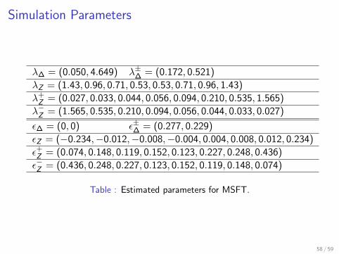
Simulation Parameters
λ∆ = (0.050, 4.649) λ±∆ = (0.172, 0.521)
λZ = (1.43, 0.96, 0.71, 0.53, 0.53, 0.71, 0.96, 1.43)
λ+Z = (0.027, 0.033, 0.044, 0.056, 0.094, 0.210, 0.535, 1.565)
λ−Z = (1.565, 0.535, 0.210, 0.094, 0.056, 0.044, 0.033, 0.027)
ε∆ = (0, 0) ε±∆ = (0.277, 0.229)
εZ = (−0.234,−0.012,−0.008,−0.004, 0.004, 0.008, 0.012, 0.234)
ε+Z = (0.074, 0.148, 0.119, 0.152, 0.123, 0.227, 0.248, 0.436)
ε−Z = (0.436, 0.248, 0.227, 0.123, 0.152, 0.119, 0.148, 0.074)
Table : Estimated parameters for MSFT.
58 / 59

Simulation Parameters
λ∆ = (0.225, 0.846) λ±∆ = (0.117, 0.049)
λZ = (1.62, 1.67, 1.81, 2.20, 2.20, 1.81, 1.67, 1.62)
λ+Z = (0.044, 0.050, 0.060, 0.066, 0.086, 0.119, 0.171, 0.331)
λ−Z = (0.331, 0.171, 0.119, 0.086, 0.066, 0.060, 0.050, 0.044)
ε∆ = (0, 0) ε±∆ = (0.534, 0.716)
εZ = (−0.252,−0.084,−0.035,−0.006, 0.006, 0.035, 0.084, 0.251)
ε+Z = (0.252, 0.329, 0.445, 0.479, 0.471, 0.541, 0.603, 0.752)
ε−Z = (0.752, 0.603, 0.541, 0.471, 0.479, 0.445, 0.329, 0.252)
Table : Estimated parameters for TEVA.
59 / 59
![High Frequency Statistical Arbitrage Modelstanford.edu/class/msande448/2019/Midterm/gr1.pdf · [1] Cartea Alvaro, Jaimungal Sebastian, Penalva José(2015). Algorithmic And High-Frequency](https://img.pdfslide.net/doc/110x75/60cc209613f87f64211c29fd/high-frequency-statistical-arbitrage-1-cartea-alvaro-jaimungal-sebastian-penalva.jpg)