Voluntary Environmental Regulation in Developing Countries · Voluntary Environmental Regulation in Developing ... third-party environmental audit. ... best practices not covered

1616 P St. NW Washington, DC 20036 202-328-5000 www.rff.org

July 2007; revised Sept. 2009 and Aug. 2010 RFF DP 07-36-REV

Voluntary Environmental Regulation in Developing Countries

Mexico’s Clean Industry Program

Al len B lackman , B id isha Lah i r i , W i l l i am P ize r ,

Mar iso l R ive ra P l an te r , and Car los Muñoz P i ña

DIS

CU

SSIO

N P

APE

R

© 2010 Resources for the Future. All rights reserved. No portion of this paper may be reproduced without permission of the authors.

Discussion papers are research materials circulated by their authors for purposes of information and discussion. They have not necessarily undergone formal peer review.

Voluntary Environmental Regulation in Developing Countries: Mexico’s Clean Industry Program

Allen Blackman, Bidisha Lahiri, William Pizer, Marisol Rivera Planter, and Carlos Muñoz Piña

Abstract Because conventional command-and-control environmental regulation often performs poorly in

developing countries, policymakers are increasingly experimenting with alternatives, including voluntary regulatory programs. Research in industrialized countries suggests that such programs are sometimes ineffective because they mainly attract relatively clean participants free-riding on unrelated pollution control investments. We use plant-level data on more than 100,000 facilities to analyze the Clean Industry Program, Mexico’s flagship voluntary regulatory initiative. We seek to identify the drivers of participation and to determine whether the program improves participants’ environmental performance. Using data from the program’s first decade, we find that plants recently fined by environmental regulators were more likely to participate, but that after graduating from the program, participants were not fined at a substantially lower rate than nonparticipants. These results suggest that although the Clean Industry Program attracted dirty plants under pressure from regulators, it did not have a large, lasting impact on their environmental performance.

Key Words: voluntary environmental regulation, duration analysis, propensity score matching, Mexico

JEL Classification Numbers: Q56, Q58, O13, O54, C41

Contents

1. Introduction ......................................................................................................................... 1

2. Background ......................................................................................................................... 3

3. Data and Variables ............................................................................................................. 5

3.1. Data .............................................................................................................................. 5

3.2. Independent Variables ................................................................................................. 7

4. Participation Model ............................................................................................................ 9

4.1. Empirical Strategy: Duration Analysis ........................................................................ 9

4.2. Modeling Fines ............................................................................................................ 9

4.3. Results ........................................................................................................................ 10

5. Impact Model .................................................................................................................... 13

5.1. Empirical Strategy: Propensity Score Matching ........................................................ 13

5.2. Results ........................................................................................................................ 16

5.3. Caveats ....................................................................................................................... 17

6. Conclusion ......................................................................................................................... 18

References .............................................................................................................................. 21

Resources for the Future Blackman et al.

1

Voluntary Environmental Regulation in Developing Countries: Mexico’s Clean Industry Program

Allen Blackman, Bidisha Lahiri, William Pizer, Marisol Rivera Planter, and Carlos Muñoz Piña∗

1. Introduction

The conventional approach to industrial pollution control is to establish laws requiring firms to cut emissions. Voluntary regulation, by contrast, provides incentives, but not mandates, for pollution control. In industrialized countries, such regulation has become popular over the past 20 years (Morgenstern and Pizer 2007; Khoeler 2007). Environmental authorities in developing countries, particularly those in Latin America, also have embraced this approach. For example, in Colombia and Chile, dozens of voluntary agreements involving thousands of firms have been signed since the mid-1990s (Blackman et al. 2009; Jiménez 2007).

Yet we know little about developing countries’ voluntary initiatives, including what drives participation and whether participation improves environmental performance. Rigorous empirical studies are rare (Blackman, In Press). This gap is significant for two reasons. First, voluntary regulation plays a particularly important role in developing countries. Whereas regulators in industrialized countries typically use it to spur overcompliance with mandatory regulation, those in developing countries generally use it to stem rampant noncompliance due to, among other factors, weak environmental management institutions and limited political will for strict enforcement (Blackman 2008). Second, findings from the considerable literature on voluntary regulation in industrialized countries may not apply to developing countries where voluntary policies are implemented in a different sociopolitical context and, as just noted, for different reasons.

∗ Blackman (corresponding author), Resources for the Future, 1616 P Street, NW, Washington, DC 20036, (202) 328–5073, [email protected]. Lahiri, Department of Economics, Spears School of Business, Oklahoma State University; Pizer, independent; Rivera Planter, Instituto Nacional de Ecología, Secretaría del Medio Ambiente y Recursos Naturales; Muñoz Piña, Instituto Nacional de Ecología, Secretaría del Medio Ambiente y Recursos Naturales.


2

To help fill this gap, this article analyzes Mexico’s flagship voluntary initiative, the National Environmental Auditing Program (Programa Nacional de Auditoria Ambiental), also known as the Clean Industry Program (Programa Industria Limpia), which provides public recognition and a temporary inspection amnesty to plants that correct deficiencies identified by a third-party environmental audit. This initiative represents one of the three main types of voluntary tools: public programs that invite firms to meet environmental performance standards.1 To our knowledge, ours is the first econometric analysis of the environmental impacts of such a policy in a developing country.2

Although its applicability is unclear, the considerable literature on industrialized countries’ voluntary environmental programs certainly raises serious questions about whether developing countries’ voluntary programs are likely to have environmental benefits. Recent literature reviews and meta analyses paint a mostly pessimistic picture (Darnall and Sides 2008; Koehler 2007; Rivera and de Leon 2010). Individual case studies suggest that at least in some instances, voluntary programs have few environmental benefits because they mainly attract already-clean firms “free riding” on their preparticipation environmental performance (Vidovic and Khanna 2007; Morgenstern and Pizer 2007). Such firms have clear incentives to join voluntary programs: the costs are relatively low because no additional investments are required to meet the program’s performance targets, and the benefits, which may include positive publicity, subsidies, and regulatory relief, can be significant.3

To evaluate the Clean Industry Program, we construct a unique data set by merging plant-level registries compiled by the Mexican Ministry of Economics and the Federal Environmental Attorney General’s Office (Procuraduría Federal de Protección al Ambiente, PROFEPA), within the Ministry of the Environment. The econometric analysis has two stages. In the first stage, we use a duration model to identify the drivers of participation in the program between 1992 and 2004. We are particularly interested in understanding whether the plants that join free-

1 Prominent examples of U.S. voluntary programs are the Environmental Protection Agency’s 33/50 and Climate Wi$e programs. The two other main types of voluntary regulation are agreements negotiated between regulatory authorities and firms, and unilateral commitments undertaken by firms (Lyon and Maxwell 2002). 2 Jiménez (2007) presents an econometric analysis of the impacts of negotiated voluntary agreements, not a voluntary public program, in Chile. Blackman and Guerrero (2010), Christmann and Taylor (2001), and Rivera (2002) present econometric analyses of participation in voluntary environmental programs in developing economies. 3 The evidence for such free riding is not unequivocal, however. In some cases, relatively dirty firms and those under pressure from regulatory authorities are more likely to participate in voluntary programs (Gamper-Rabindran 2006; Sam and Innes 2008; Short and Toffel 2007).


3

ride on their preparticipation environmental performance. Because reliable direct measures of environmental performance are not available, we use the incidence of PROFEPA fines as a proxy. Ex ante, it is not clear that fines drive participation. Even in industrialized countries with robust regulatory pressure, the links between environmental performance, regulatory fines, and participation in voluntary programs are tentative (Arora and Cason 1996; Gamper-Rabindran 2006). In Mexico, where the regulatory pressure is generally weaker because of a lack of manpower, expertise, and political will (OECD 2003; Gilbreath 2003; Brizzi and Ahmed 2001), one might reasonably expect these links to be even more uncertain.

In the second stage of our analysis, we use propensity score matching to measure the impact of the Clean Industry Program on participants’ environmental performance; that is, we compare the average performance of a sample of participants with that of a matched sample of nonparticipants. Here, too, we use the incidence of PROFEPA fines as a proxy for environmental performance. We rely on the duration model estimated in the first stage to generate propensity scores.

Our first-stage duration analysis indicates that plants recently fined by PROFEPA were more likely to join the Clean Industry Program, all other things equal. However, the second-stage matching analysis shows that after graduating from the program, participants were not fined at a substantially lower rate than nonparticipants. These results suggest that although the program attracted dirty plants under pressure from regulators, it did not have a large, lasting impact on their environmental performance.

2. Background

Launched in 1992, the Clean Industry Program is one of the three pillars of PROFEPA’s enforcement strategy, along with inspections and citizen complaints. Plants volunteering to join the program pay for a environmental audit by an accredited third-party inspector. The audit assesses both the plant’s compliance with all relevant environmental regulations (including those for which regulators other than PROFEPA are responsible) and its adherence to international environmental management best practices not covered by regulations.4 Following the audit, the

4 PROFEPA is responsible for enforcing hazardous waste, air pollution, and natural resource regulations, including for forestry and fisheries (OECD 2003). The National Water Commission (Comisión Nacional del Agua, CNA) is charged with enforcing water quality regulation. Local governments also have some enforcement powers over water pollution and solid waste. In practice, the division of responsibilities among PROFEPA, CNA, and local


4

plant negotiates an action plan with PROFEPA wherein it agrees to correct all deficiencies identified in the audit by an agreed-upon deadline, which for most plants is more than two years after the audit.5 PROFEPA, in exchange, agrees not to penalize the plant while these improvements are being made. If the plant fulfills all the terms of its action plan, PROFEPA awards it a Clean Industry Certificate that is valid for two years. These certificates are commonly used in domestic and international marketing campaigns and are considered a major benefit of participation (Alvarez-Larraurri and Fogel 2008; Harvard University 2000). In addition, PROFEPA agrees not to inspect the plant for two years except in the event of an industrial accident or public complaint. When the Clean Industry Certificate expires, the plant must repeat the auditing process to be recertified. Hence, like many voluntary initiatives, the Clean Industry Program provides both carrots and sticks to encourage participation.

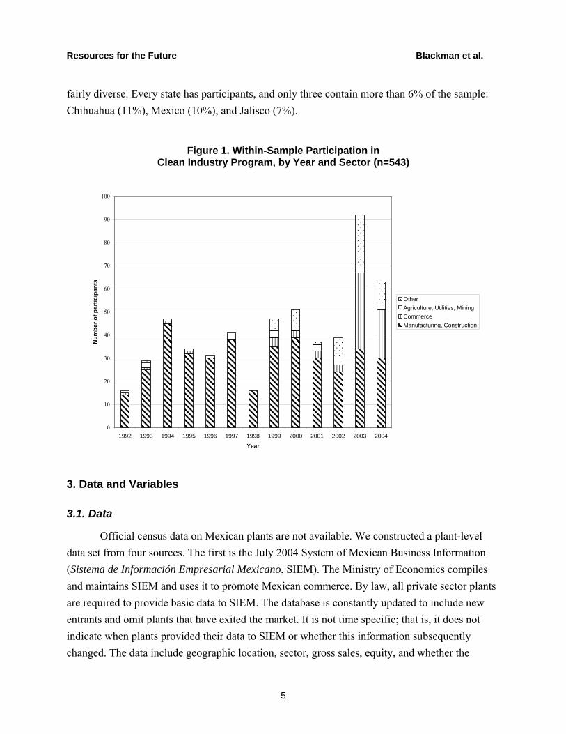
Participation in the Clean Industry Program grew from 78 plants in 1992 to 7,616 plants in 2008 (PROFEPA 2009). For most of the 1990s, the Clean Industry Program focused on recruiting large often publicly owned plants in sectors that PROFEPA classified as “at risk” for industrial accidents, such as cement, chemicals, electronics, oil refining, and pharmaceuticals. In 2001, the program’s mandate was changed from mitigating industrial risk to environmental protection, and as a result, more nonmanufacturing facilities began to participate. PROFEPA also has intensified efforts to attract small and medium enterprises (Alvarez-Larraurri and Fogel 2008). Figure 1 shows participation by sector and year between 1992 and 2004 for the sample of 543 Clean Industry participants included in our empirical analysis.6 It reflects major trends for the population of participants during this period (Alvarez-Larraurro and Fogel 2008): a dip in participation rates in the mid-1990s followed by a steep rise in 2003 and 2004, and increasing participation by plants in sectors other than manufacturing and construction following the change in the program’s mandate in 2001.7 Geographically, participants in our regression sample were

governments has been somewhat confused and contentious, particularly in the first years after PROFEPA’s creation in 1992 (Blackman and Sisto 2006; Gilbreath 2003). 5 According to Harvard University (2000, 5) “It is important to note that Mexico’s voluntary audit program is much more than a system for verifying compliance ... In many instances, international standards and ‘best practices’ guide the auditors recommendations and PROFEPA’s negotiated agreement with the facilities.” 6 The selection of the sample is discussed in Section 3.1. 7 The dip in participation in the 1990s was partly due to an economic crisis and partly due to problems with the program’s design and administration, which were addressed by subsequent administrative reforms. These problems included confusion about terms of reference for audits, their high costs, and overall lack of transparency (Alvarez-Larraurri and Fogel 2008; Harvard University 2000).


5

fairly diverse. Every state has participants, and only three contain more than 6% of the sample: Chihuahua (11%), Mexico (10%), and Jalisco (7%).

Figure 1. Within-Sample Participation in

Clean Industry Program, by Year and Sector (n=543)

0

10

20

30

40

50

60

70

80

90

100

1992 1993 1994 1995 1996 1997 1998 1999 2000 2001 2002 2003 2004

Year

Num

ber o

f par

ticip

ants

OtherAgriculture, Utilities, MiningCommerceManufacturing, Construction

3. Data and Variables

3.1. Data

Official census data on Mexican plants are not available. We constructed a plant-level data set from four sources. The first is the July 2004 System of Mexican Business Information (Sistema de Información Empresarial Mexicano, SIEM). The Ministry of Economics compiles and maintains SIEM and uses it to promote Mexican commerce. By law, all private sector plants are required to provide basic data to SIEM. The database is constantly updated to include new entrants and omit plants that have exited the market. It is not time specific; that is, it does not indicate when plants provided their data to SIEM or whether this information subsequently changed. The data include geographic location, sector, gross sales, equity, and whether the


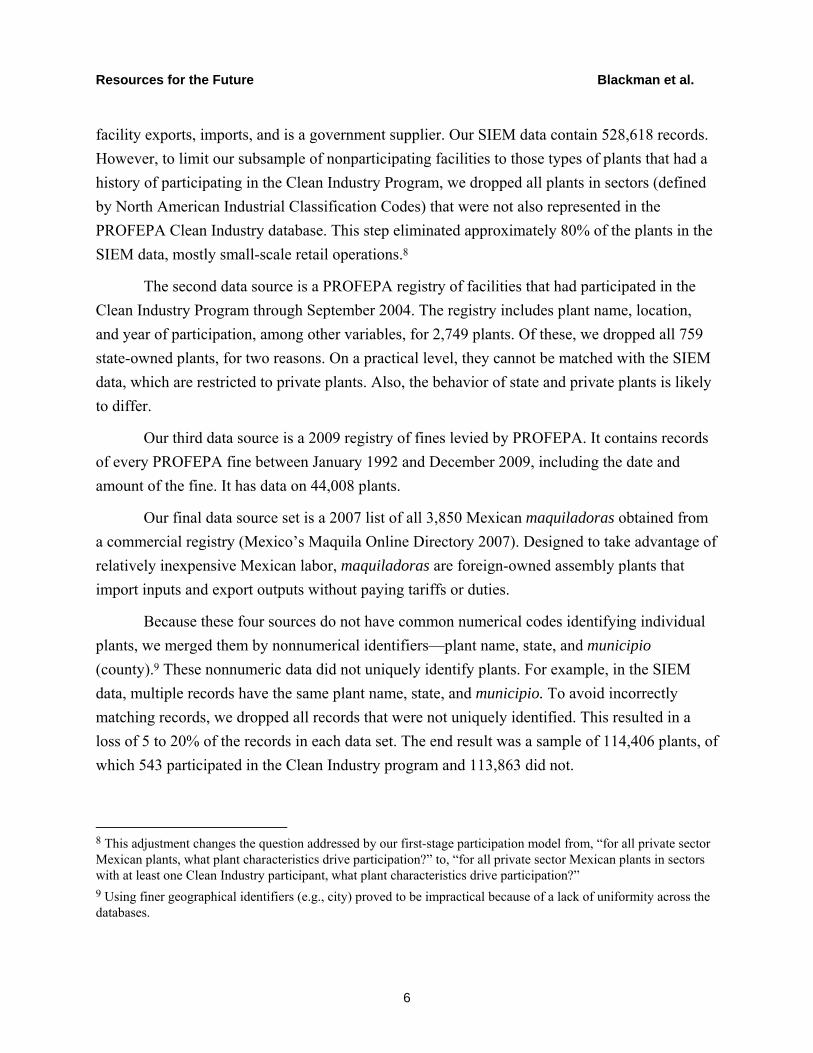
6

facility exports, imports, and is a government supplier. Our SIEM data contain 528,618 records. However, to limit our subsample of nonparticipating facilities to those types of plants that had a history of participating in the Clean Industry Program, we dropped all plants in sectors (defined by North American Industrial Classification Codes) that were not also represented in the PROFEPA Clean Industry database. This step eliminated approximately 80% of the plants in the SIEM data, mostly small-scale retail operations.8

The second data source is a PROFEPA registry of facilities that had participated in the Clean Industry Program through September 2004. The registry includes plant name, location, and year of participation, among other variables, for 2,749 plants. Of these, we dropped all 759 state-owned plants, for two reasons. On a practical level, they cannot be matched with the SIEM data, which are restricted to private plants. Also, the behavior of state and private plants is likely to differ.

Our third data source is a 2009 registry of fines levied by PROFEPA. It contains records of every PROFEPA fine between January 1992 and December 2009, including the date and amount of the fine. It has data on 44,008 plants.

Our final data source set is a 2007 list of all 3,850 Mexican maquiladoras obtained from a commercial registry (Mexico’s Maquila Online Directory 2007). Designed to take advantage of relatively inexpensive Mexican labor, maquiladoras are foreign-owned assembly plants that import inputs and export outputs without paying tariffs or duties.

Because these four sources do not have common numerical codes identifying individual plants, we merged them by nonnumerical identifiers—plant name, state, and municipio (county).9 These nonnumeric data did not uniquely identify plants. For example, in the SIEM data, multiple records have the same plant name, state, and municipio. To avoid incorrectly matching records, we dropped all records that were not uniquely identified. This resulted in a loss of 5 to 20% of the records in each data set. The end result was a sample of 114,406 plants, of which 543 participated in the Clean Industry program and 113,863 did not.

8 This adjustment changes the question addressed by our first-stage participation model from, “for all private sector Mexican plants, what plant characteristics drive participation?” to, “for all private sector Mexican plants in sectors with at least one Clean Industry participant, what plant characteristics drive participation?” 9 Using finer geographical identifiers (e.g., city) proved to be impractical because of a lack of uniformity across the databases.


7

3.2. Independent Variables

3.2.1. Time-Varying Independent Variables: Fines

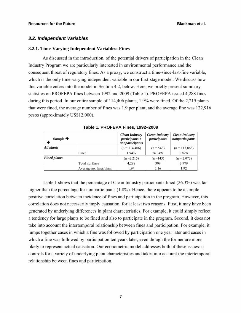
As discussed in the introduction, of the potential drivers of participation in the Clean Industry Program we are particularly interested in environmental performance and the consequent threat of regulatory fines. As a proxy, we construct a time-since-last-fine variable, which is the only time-varying independent variable in our first-stage model. We discuss how this variable enters into the model in Section 4.2, below. Here, we briefly present summary statistics on PROFEPA fines between 1992 and 2009 (Table 1). PROFEPA issued 4,288 fines during this period. In our entire sample of 114,406 plants, 1.9% were fined. Of the 2,215 plants that were fined, the average number of fines was 1.9 per plant, and the average fine was 122,916 pesos (approximately US$12,000).

Table 1. PROFEPA Fines, 1992–2009

Sample

Clean Industry participants +

nonparticipants

Clean Industry participants

Clean Industry nonparticipants

All plants (n = 114,406) (n = 543) (n = 113,863) Fined 1.94% 26.34% 1.82% Fined plants (n =2,215) (n =143) (n = 2,072) Total no. fines 4,288 309 3,979 Average no. fines/plant 1.94 2.16 1.92

Table 1 shows that the percentage of Clean Industry participants fined (26.3%) was far higher than the percentage for nonparticipants (1.8%). Hence, there appears to be a simple positive correlation between incidence of fines and participation in the program. However, this correlation does not necessarily imply causation, for at least two reasons. First, it may have been generated by underlying differences in plant characteristics. For example, it could simply reflect a tendency for large plants to be fined and also to participate in the program. Second, it does not take into account the intertemporal relationship between fines and participation. For example, it lumps together cases in which a fine was followed by participation one year later and cases in which a fine was followed by participation ten years later, even though the former are more likely to represent actual causation. Our econometric model addresses both of these issues: it controls for a variety of underlying plant characteristics and takes into account the intertemporal relationship between fines and participation.


8

3.2.2. Time-Invariant Independent Variables

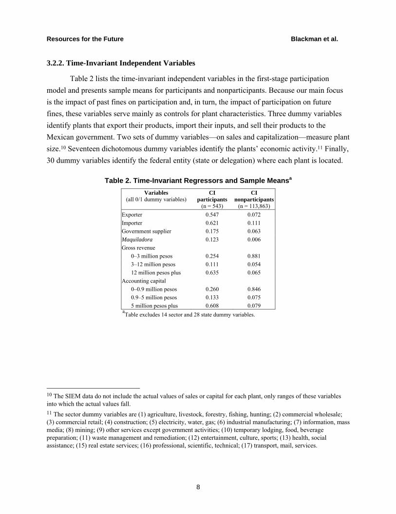
Table 2 lists the time-invariant independent variables in the first-stage participation model and presents sample means for participants and nonparticipants. Because our main focus is the impact of past fines on participation and, in turn, the impact of participation on future fines, these variables serve mainly as controls for plant characteristics. Three dummy variables identify plants that export their products, import their inputs, and sell their products to the Mexican government. Two sets of dummy variables—on sales and capitalization—measure plant size.10 Seventeen dichotomous dummy variables identify the plants’ economic activity.11 Finally, 30 dummy variables identify the federal entity (state or delegation) where each plant is located.

Table 2. Time-Invariant Regressors and Sample Meansa Variables

(all 0/1 dummy variables)

CI participants

(n = 543)

CI nonparticipants

(n = 113,863) Exporter 0.547 0.072 Importer 0.621 0.111 Government supplier 0.175 0.063 Maquiladora 0.123 0.006 Gross revenue

0–3 million pesos 0.254 0.881 3–12 million pesos 0.111 0.054 12 million pesos plus 0.635 0.065

Accounting capital 0–0.9 million pesos 0.260 0.846 0.9–5 million pesos 0.133 0.075 5 million pesos plus 0.608 0.079

aTable excludes 14 sector and 28 state dummy variables.

10 The SIEM data do not include the actual values of sales or capital for each plant, only ranges of these variables into which the actual values fall. 11 The sector dummy variables are (1) agriculture, livestock, forestry, fishing, hunting; (2) commercial wholesale; (3) commercial retail; (4) construction; (5) electricity, water, gas; (6) industrial manufacturing; (7) information, mass media; (8) mining; (9) other services except government activities; (10) temporary lodging, food, beverage preparation; (11) waste management and remediation; (12) entertainment, culture, sports; (13) health, social assistance; (15) real estate services; (16) professional, scientific, technical; (17) transport, mail, services.


9

4. Participation Model

4.1. Empirical Strategy: Duration Analysis

We use a duration model to estimate a hazard rate—the conditional probability that a plant in our data set joins the Clean Industry Program at time t, given that it has not already joined and given its characteristics at time t.12 We use a duration model for two reasons. First, it explicitly accounts for the intertemporal relationship between fines and participation, which, as discussed above, helps determine whether fines actually cause participation. Second, it avoids the problem of right censoring that would arise in a cross-sectional dichotomous choice model if some plants that were not participating in September 2004 (when our participation panel ends) subsequently joined the program. A duration approach circumvents this problem by estimating the conditional probability of participation in each period. We use a Cox (1975) proportional hazard model because it does not require parametric assumptions about the time-dependence of the probability density function. We use years as our temporal unit of analysis. Although we know the day on which plants were fined, we know only the year in which plants joined the program.13 Finally, note that although plants can and do participate in the Clean Industry Program more than once, our duration model seeks to explain the decision to participate for the first time. As is standard practice with duration models, observations (here, plants) are dropped from the regression sample after their first “failure” (here, participation).

4.2. Modeling Fines

We use an eight-year third-order polynomial to fit the relationship over time between a fine and the probability of joining the Clean Industry Program. After eight years have passed, we assume the effect of the fine is constant (and likely zero). We therefore include three fine variables in the model: the number of years since the most recent fine (TF), the square of that number (TF^2), and the cube of that number (TF^3). All these variables are set equal to zero if

12 For an introduction, see Kiefer (1998). 13 Our use of years as a temporal unit of analysis raises questions about whether time aggregation bias is a problem, and whether a discrete-time representation might be more appropriate. In general, time aggregation bias is a problem only when hazard rates are high and/or the periods of measurement are long—that is, when a large number of failure events in a given interval erode the underlying population of units at risk of failure (Petersen 1991). This is not the case in our sample: the number of plants joining the program in any given year is always quite small relative to the number of nonparticipating plants.


10

the most recent fine occurred more than eight years earlier or if a fine never occurred. We also include a dichotomous dummy variable set equal to one if the plant was ever fined at any time prior to the current period (TFP). This dummy variable picks up the permanent effect of ever having been fined, while the three other fine variables pick up the transient effect of a recent fine. Together, the estimated coefficients for the four fine variables map out the effect on the conditional probability of joining the program (hazard rate) as a function of the time since the most recent fine.14

4.3. Results

4.3.1. Time-Varying Independent Variable: Fines

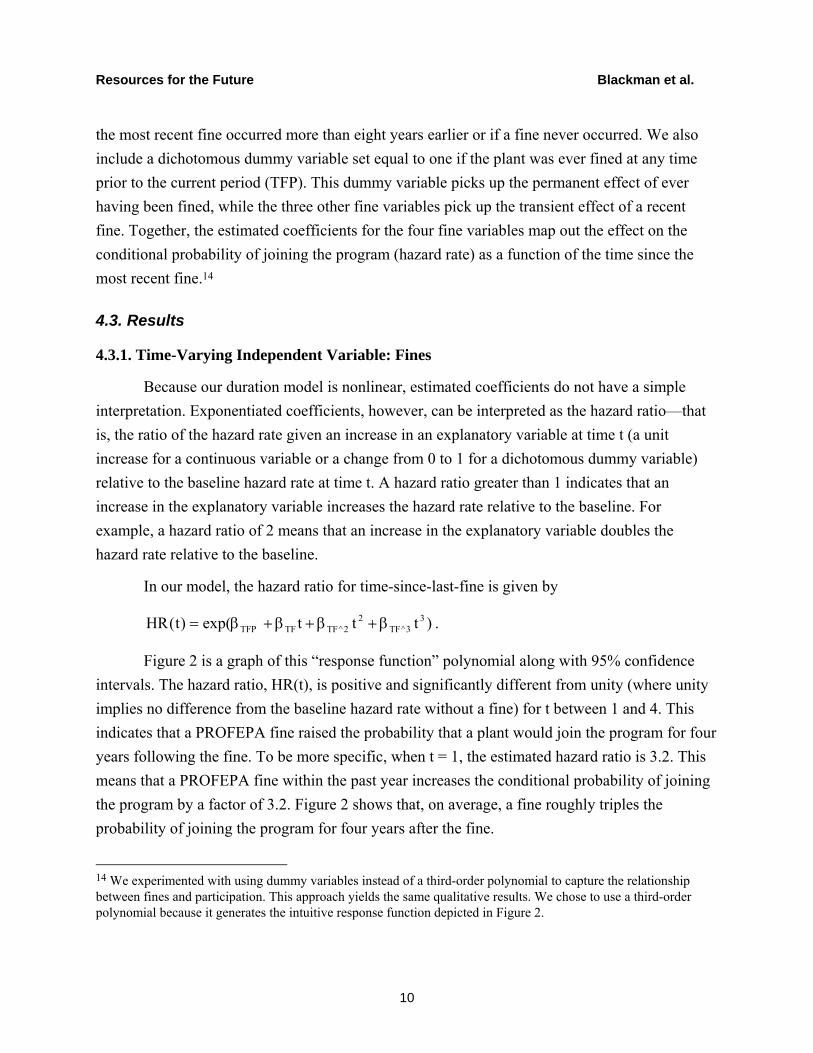
Because our duration model is nonlinear, estimated coefficients do not have a simple interpretation. Exponentiated coefficients, however, can be interpreted as the hazard ratio—that is, the ratio of the hazard rate given an increase in an explanatory variable at time t (a unit increase for a continuous variable or a change from 0 to 1 for a dichotomous dummy variable) relative to the baseline hazard rate at time t. A hazard ratio greater than 1 indicates that an increase in the explanatory variable increases the hazard rate relative to the baseline. For example, a hazard ratio of 2 means that an increase in the explanatory variable doubles the hazard rate relative to the baseline.

In our model, the hazard ratio for time-since-last-fine is given by

)tttexp()t(HR 33^TF

22^TFTFTFP β+β+β+β= .

Figure 2 is a graph of this “response function” polynomial along with 95% confidence intervals. The hazard ratio, HR(t), is positive and significantly different from unity (where unity implies no difference from the baseline hazard rate without a fine) for t between 1 and 4. This indicates that a PROFEPA fine raised the probability that a plant would join the program for four years following the fine. To be more specific, when t = 1, the estimated hazard ratio is 3.2. This means that a PROFEPA fine within the past year increases the conditional probability of joining the program by a factor of 3.2. Figure 2 shows that, on average, a fine roughly triples the probability of joining the program for four years after the fine.

14 We experimented with using dummy variables instead of a third-order polynomial to capture the relationship between fines and participation. This approach yields the same qualitative results. We chose to use a third-order polynomial because it generates the intuitive response function depicted in Figure 2.


11

Figure 2. Hazard Ratio (Hazard Rate with/without Fine) for Probability of Joining Clean Industry Program as Function of Years Since Last Fine

0.0

1.0

2.0

3.0

4.0

5.0

1 2 3 4 5 6

Years since last fine

Haz

ard

rati

o

estimated effect

95% conf. interval

A potential concern about our analysis is that fines variables could, in principle, be endogenous if they are correlated with unobserved plant characteristics that affect participation.15 Although such endogeneity cannot be ruled out, it is unlikely to be driving the observed correlation between fines and participation, since endogeneity would generate a response that did not change over time, rather than a response that diminishes in magnitude (Figure 2).16

15 For example, aside from our sector dummies, our covariates do not include a precise measure of the complexity of the production process, so complexity is partly unobserved. It could be that complex plants are more likely to be fined because they have a higher potential for violating environmental regulations and are also more likely to participate in the program because they tend to employ educated and sophisticated managers. If this were actually true, then fines would be endogenous. 16 Intraclass correlation is a second potential concern. Some plants in our regression sample are owned by the same firm. Presumably, in some cases, the decision to participate is made at the firm level. But in other cases, it is clearly made at the plant level—some plants owned by the same firm do not make the same participation decision. In cases where the participation decision is made at the firm level, our data may exhibit intraclass correlation. Ideally, we would correct for this correlation using clustered standard errors. However, we are not able to do that for two reasons. First, we cannot reliably identify cases where the participation decision is made at the firm versus the plant level. Second, our indicator of common ownership is unreliable. The only data we can use to determine whether plants share a common owner is their names. But in some cases, plants with different names are owned by the same parent firm.


12

Hence, the results summarized in Figure 2 suggest a causal relationship between fines and participation in the program. In particular, the fact that the positive and significant effect of fines on the hazard ratio diminishes over time suggests that fines drive participation.

4.3.2. Time-Invariant Independent Variables

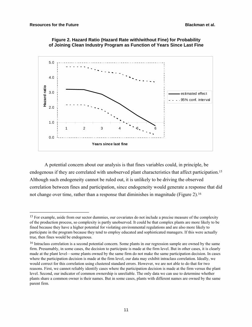
Table 3 presents regression results for the time-invariant regressors. Hazard ratios for the exporter, importer, and government supplier dummy variables are all positive and significant at the 1% level. They indicate that plants selling their goods in overseas markets were 1.8 times more likely to participate in the Clean Industry Program, those importing foreign inputs were 1.7 times more likely, and those selling products to government were 1.4 times more likely. The hazard ratio for the maquiladora dummy is not significant.

Table 3. Regression Results for Cox Proportional Hazard Model of Participation in Clean Industry Program, 1992–2004 (n = 114,406);

Time-Invariant Regressorsa

Variable Hazard Ratio S.E. Exporter 1.823*** 0.252 Importer 1.738*** 0.254 Government supplier 1.370*** 0.170 Maquiladora 1.175 0.184 Gross revenue

3–12 million pesos 2.225*** 0.402 12 million pesos plus 4.102*** 0.672

Accounting capital 0.9–5 million pesos 1.966*** 0.330 5 million pesos plus 3.144*** 0.486

Log likelihood -5201.771 aModel includes 14 sector dummy variables, 28 state dummy variables, and 4 fines variables, which are omitted from the table. See Figure 2 for fines variables results. ***Significant at 1% level

Hazard ratios for the sales and capital dummies suggest that larger plants were more likely to participate. Hazard ratios for the sales dummies indicate that compared with plants with less than 3 million pesos in sales (the reference group), those with 3 million to 12 million pesos in sales were 2.2 times more likely to participate, and those with more than 12 million pesos in sales were 4.1 times more likely. Similarly, hazard ratios for the capitalization dummies indicate that compared with plants with less than 0.9 million pesos in capital, those with 0.9 million to 5 million pesos in capital were 2.0 times more likely to participate, and those with more than 5 million pesos in capital were 3.1 times more likely.


13

For the sector fixed effects, the reference sector is educational services. Compared with plants in this sector, those in mass media were less likely to join and those in mining were more likely to join. For the state fixed effects, the reference states are Campeche, Chiapas, Guerrero, and Colima. Compared with plants in these states, those in Mexico City were less likely to participate, and those in Aguascalientes, Chihuahua, Morelos, Oaxaca, Tlaxcala, and Zacatecas were more likely.

5. Impact Model

5.1. Empirical Strategy: Propensity Score Matching

Analyzing the Clean Industry Program’s impact on participants’ environmental performance is challenging for two reasons. First, reasonably accurate, direct measurements of plants’ environmental performance (such as data on emissions of air and water pollutants) are unavailable. As a proxy, we again use our PROFEPA fines data—specifically, the average number of fines assessed per year after the inspection amnesty ends. As long as dirty plants are fined more, and more often, than clean ones, these averages will be negatively correlated with environmental performance.

The second challenge is a general problem in evaluating a program’s impact on a performance indicator (Rubin 1974; Holland 1986). Ideally, impact would be measured by comparing each agent’s performance with program participation and without it. However, we never actually observe both. In practice, therefore, program impact is often measured by comparing the average performance of participants with that of a matched control sample of nonparticipants that have very similar observable characteristics. The average performance of the matched sample proxies for the unobserved counterfactual—what participants performance would have been had they not participated. Matching controls for nonrandom selection into the program (Rosenbaum and Rubin 1983; Ferraro et al. 2007; List et al. 2003; Dehejia and Wahba 2002).

Specifically, our measure of the impact of the Clean Industry Program—the average treatment effect on the treated (ATT)—is the difference between the average number of fines per year incurred by participants and by a matched sample of nonparticipants during an outcome period that depends on the timing of participation. For each matched set of plants, the first year of this period is the eighth year after the participant joined the Clean Industry Program (i.e., was audited) and the last year is 2009, the last full year of our fines panel. As discussed below, the eight-year lag controls for the inspection amnesty granted to participants.


14

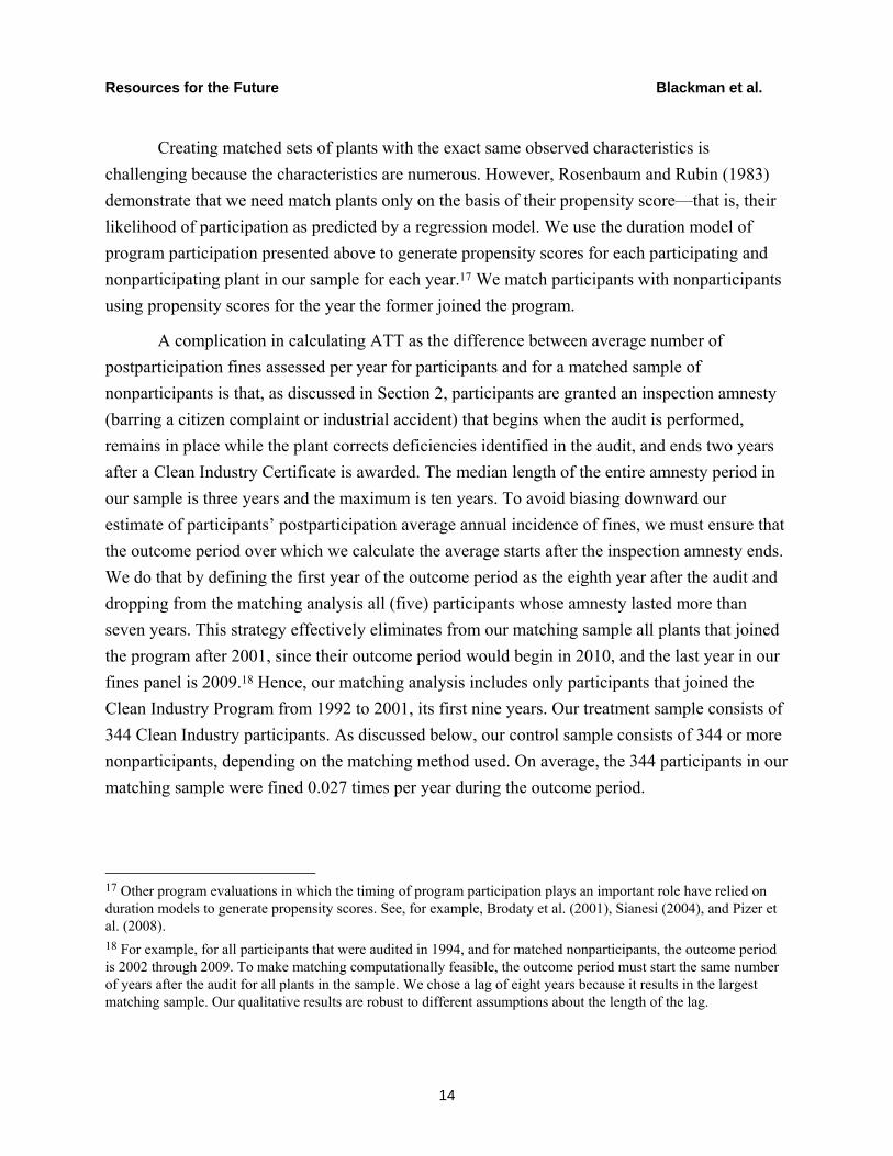
Creating matched sets of plants with the exact same observed characteristics is challenging because the characteristics are numerous. However, Rosenbaum and Rubin (1983) demonstrate that we need match plants only on the basis of their propensity score—that is, their likelihood of participation as predicted by a regression model. We use the duration model of program participation presented above to generate propensity scores for each participating and nonparticipating plant in our sample for each year.17 We match participants with nonparticipants using propensity scores for the year the former joined the program.

A complication in calculating ATT as the difference between average number of postparticipation fines assessed per year for participants and for a matched sample of nonparticipants is that, as discussed in Section 2, participants are granted an inspection amnesty (barring a citizen complaint or industrial accident) that begins when the audit is performed, remains in place while the plant corrects deficiencies identified in the audit, and ends two years after a Clean Industry Certificate is awarded. The median length of the entire amnesty period in our sample is three years and the maximum is ten years. To avoid biasing downward our estimate of participants’ postparticipation average annual incidence of fines, we must ensure that the outcome period over which we calculate the average starts after the inspection amnesty ends. We do that by defining the first year of the outcome period as the eighth year after the audit and dropping from the matching analysis all (five) participants whose amnesty lasted more than seven years. This strategy effectively eliminates from our matching sample all plants that joined the program after 2001, since their outcome period would begin in 2010, and the last year in our fines panel is 2009.18 Hence, our matching analysis includes only participants that joined the Clean Industry Program from 1992 to 2001, its first nine years. Our treatment sample consists of 344 Clean Industry participants. As discussed below, our control sample consists of 344 or more nonparticipants, depending on the matching method used. On average, the 344 participants in our matching sample were fined 0.027 times per year during the outcome period.

17 Other program evaluations in which the timing of program participation plays an important role have relied on duration models to generate propensity scores. See, for example, Brodaty et al. (2001), Sianesi (2004), and Pizer et al. (2008). 18 For example, for all participants that were audited in 1994, and for matched nonparticipants, the outcome period is 2002 through 2009. To make matching computationally feasible, the outcome period must start the same number of years after the audit for all plants in the sample. We chose a lag of eight years because it results in the largest matching sample. Our qualitative results are robust to different assumptions about the length of the lag.


15

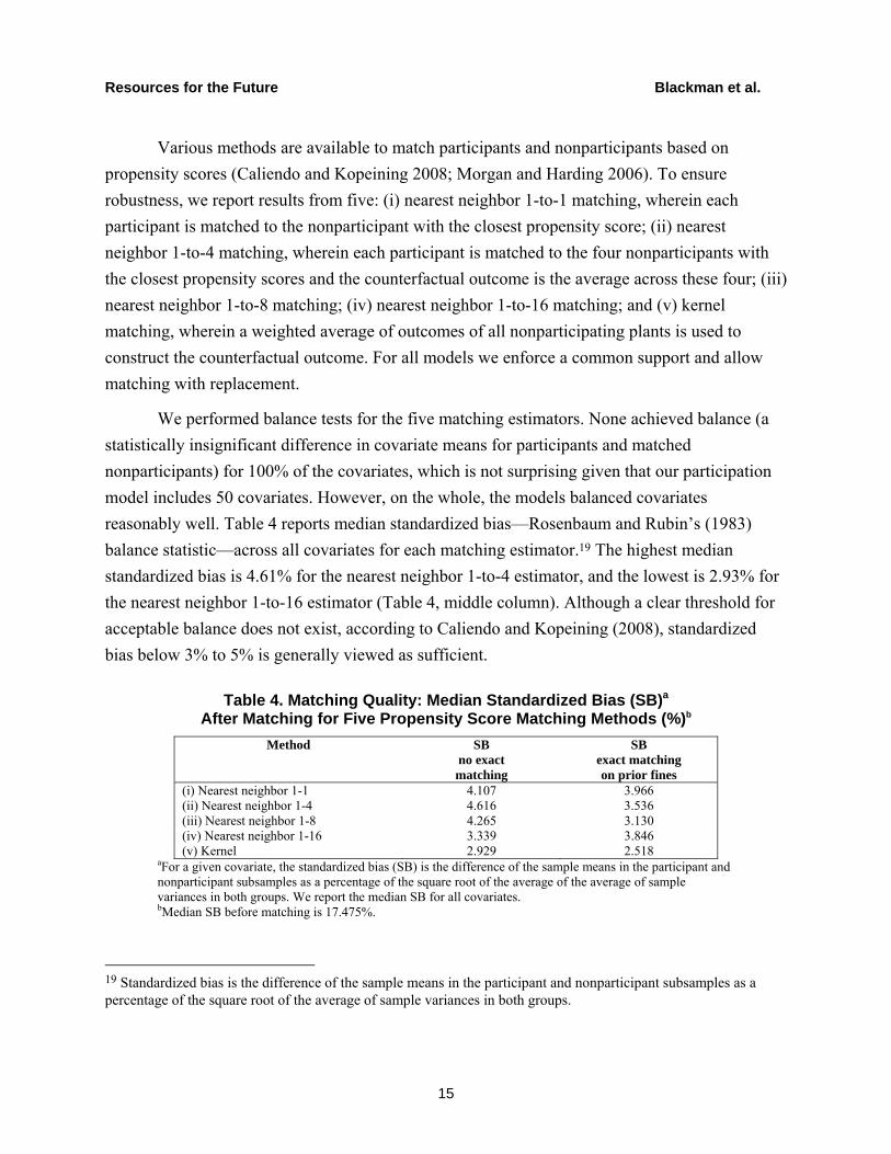
Various methods are available to match participants and nonparticipants based on propensity scores (Caliendo and Kopeining 2008; Morgan and Harding 2006). To ensure robustness, we report results from five: (i) nearest neighbor 1-to-1 matching, wherein each participant is matched to the nonparticipant with the closest propensity score; (ii) nearest neighbor 1-to-4 matching, wherein each participant is matched to the four nonparticipants with the closest propensity scores and the counterfactual outcome is the average across these four; (iii) nearest neighbor 1-to-8 matching; (iv) nearest neighbor 1-to-16 matching; and (v) kernel matching, wherein a weighted average of outcomes of all nonparticipating plants is used to construct the counterfactual outcome. For all models we enforce a common support and allow matching with replacement.

We performed balance tests for the five matching estimators. None achieved balance (a statistically insignificant difference in covariate means for participants and matched nonparticipants) for 100% of the covariates, which is not surprising given that our participation model includes 50 covariates. However, on the whole, the models balanced covariates reasonably well. Table 4 reports median standardized bias—Rosenbaum and Rubin’s (1983) balance statistic—across all covariates for each matching estimator.19 The highest median standardized bias is 4.61% for the nearest neighbor 1-to-4 estimator, and the lowest is 2.93% for the nearest neighbor 1-to-16 estimator (Table 4, middle column). Although a clear threshold for acceptable balance does not exist, according to Caliendo and Kopeining (2008), standardized bias below 3% to 5% is generally viewed as sufficient.

Table 4. Matching Quality: Median Standardized Bias (SB)a After Matching for Five Propensity Score Matching Methods (%)b

Method SB no exact matching

SB exact matching on prior fines

(i) Nearest neighbor 1-1 4.107 3.966 (ii) Nearest neighbor 1-4 4.616 3.536 (iii) Nearest neighbor 1-8 4.265 3.130 (iv) Nearest neighbor 1-16 3.339 3.846 (v) Kernel 2.929 2.518

aFor a given covariate, the standardized bias (SB) is the difference of the sample means in the participant and nonparticipant subsamples as a percentage of the square root of the average of the average of sample variances in both groups. We report the median SB for all covariates. bMedian SB before matching is 17.475%.

19 Standardized bias is the difference of the sample means in the participant and nonparticipant subsamples as a percentage of the square root of the average of sample variances in both groups.


16

Because the fines covariates are likely to be particularly important in explaining subsequent fines during the outcome period, in a second set of models, we enforce exact matching on a dummy variable indicating whether the plant had been fined by PROFEPA prior to the outcome period. Hence, these models ensure that participants that were fined before the outcome period are matched with nonparticipants that also were fined before this period, and vice versa. Median standardized bias for the exact matching models ranges from 3.97% to 2.52% (Table 4, last column).

Calculating standard errors for ATT is not straightforward because they should, in principle, account for the fact that propensity scores are estimated and for the imputation of the common support (Heckman et al. 1998). Therefore, we bootstrap standard errors using 500 replications.

5.2. Results

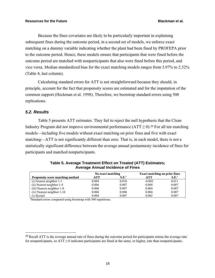
Table 5 presents ATT estimates. They fail to reject the null hypothesis that the Clean Industry Program did not improve environmental performance (ATT ≥ 0).20 For all ten matching models—including five models without exact matching on prior fines and five with exact matching—ATT is not significantly different than zero. That is, in each model, there is not a statistically significant difference between the average annual postamnesty incidence of fines for participants and matched nonparticipants.

Table 5. Average Treatment Effect on Treated (ATT) Estimates; Average Annual Incidence of Fines

No exact matching Exact matching on prior fines Propensity score matching method ATT S.E.a ATT S.E.a

(i) Nearest neighbor 1-1 0.004 0.010 -0.003 0.011 (ii) Nearest neighbor 1-4 0.006 0.007 0.004 0.007 (iii) Nearest neighbor 1-8 0.006 0.007 0.004 0.007 (iv) Nearest neighbor 1-16 0.004 0.006 0.004 0.007 (v) Kernel 0.004 0.007 0.002 0.007

aStandard errors computed using bootstrap with 500 repetitions.

20 Recall ATT is the average annual rate of fines during the outcome period for participants minus the average rate for nonparticipants, so ATT ≥ 0 indicates participants are fined at the same, or higher, rate than nonparticipants.


17

5.3. Caveats

Although the results from the matching analysis suggest that the Clean Industry Program did not have a lasting effect on environmental performance, three caveats are in order. First, the limited number of observations and variability in our outcome data bound the precision of our hypothesis test. As a result, we cannot infer that the Clean Industry Program did not reduce at all the rate at which participants were subsequently fined, only that it did reduce it by a large amount. Specifically, we can reject the hypothesis that the program reduced this fine rate by more than 46% (ATT ≤ 46% of participants’ postamnesty fine rate).21

Second, as noted above, our matching sample includes plants that joined in the first nine years of the program, mostly before the year 2001 reforms (discussed in Section 2) that shifted the program’s focus from industrial safety to environmental management and aimed to improve program functioning. Were the requisite data available, an analysis of a more recent cohort of participants might generate a different conclusion.

Third, ATT could be biased upward (i.e., no benefit from participation) if regulatory monitoring that leads to fines was more stringent for participants than for nonparticipants during the outcome period. If this were the case, then improvements in environmental performance due to participation might not be reflected in a lower incidence of PROFEPA fines, simply because participants were more closely inspected and therefore more frequently fined than similar nonparticipants. Unfortunately, the hard data on PROFEPA inspections needed to test and control for the stringency of monitoring are not available.22 Softer evidence is equivocal.

21 To see this, first note the t-score used to test hypotheses about ATT is ( ) ( )CT XXCT XXt

−σ−=

where TX and CX are the mean outcomes for the treatment and control groups, the numerator therefore is the ATT, and ( )CT XX −

σ is the standard error of ATT. If we know TX , ( )CT XX −

σ , and the t-score needed to reject the null hypothesis that the Clean Industry Program did not reduce the rate at which participants were subsequently fined (ATT ≥ 0), which we will denote t*, then we can calculate *

CX , the mean outcome for the control group needed to reject this null hypothesis. That is, ( )CT XX

*T

*C tXX

−σ+= . The one-sided t-score needed to reject the null at 5% given 343 degrees of

freedom is 1.649. As noted above, TX is 0.027. ( )CT XX −σ

depends on the matching model used. As a result, each

matching model is associated with a different *CX . The average for all ten matching models is 0.040. Thus, to reject

the null hypothesis, CX would need to be 0.040, which is 46% [(0.040-0.027)/0.027)] higher than TX . Since CX serves as our counterfactual (i.e., what the mean fine rate for participants would have been had they not participated), an equivalent interpretation is that participation in the Clean Industry Program would need to reduce the mean fine rate by at least 46%. Hence, our results allow us to reject any hypothesis that Clean Industry program reduced participants’ incidence of fines by more than 46%. 22 An earlier version of this paper used inspection data in a duration model of program participation. However, these data included only inspections that identified a regulatory violation, not inspections that did not turn up violations. Such inspections are highly correlated with fines. Not surprisingly, the duration results are qualitatively equivalent to those from the fines model.


18

On one hand, some anecdotal evidence suggests that participants were monitored more closely than nonparticipants during the outcome period. As noted in Section 2, when participants’ Clean Industry Certificates expire after two years, they can get “recertified” by commissioning a new third-party audit, negotiating a new action plan with PROFEPA, and submitting to a new follow-up PROFEPA inspection. Recertified plants may have been subjected to relatively stringent monitoring during the recertification process: Clean Industry audits cover regulatory and extraregulatory standards for air pollution, water pollution, and hazardous waste, whereas normal PROFEPA inspections typically focus on regulatory standards for the one or two pollution issues most prevalent in the plant’s economic sector (Barrera 2009; Ortiz 2009).

But an argument can also be made that monitoring for participants was less stringent than for nonparticipants during the outcome period. Recertified plants were granted an inspection amnesty (barring a citizen complaint or industrial accident) lasting from their second audit until two years after their second Clean Industry Certificate was awarded. Presumably, monitoring during this period was minimal. Also, PROFEPA may have “rewarded” successful graduates of the Clean Industry Program with less stringent monitoring just as participants in the U.S.Environmental Protection Agency’s voluntary audit program are rewarded with relaxed oversight (Toffel and Short 2008; Stafford 2007).

6. Conclusion

We have used data on some 114,000 industrial facilities and other businesses in Mexico to evaluate the Clean Industry Program, Mexico’s flagship voluntary regulatory program. The first stage of our analysis focused on identifying the drivers of participation in the program, and the second stage focused on determining whether it improves participants’ environmental performance.

To analyze participation, we used a duration model because it explicitly accounts for the timing of the dependent variable (participation) and the main independent variable of interest (fines) and because it controls for right censoring. Our results suggest that regulatory fines do motivate participation in the program: a fine roughly triples the probability of participation for three years after it is assessed. Hence, the Clean Industry Program does not simply consist of already-clean plants. Rather, it has attracted dirty plants under pressure from regulators. The analysis also shows that certain types of plants—those that sell their goods in overseas markets and to government suppliers, use imported inputs, are large, and are in certain sectors and states—are more likely to participate.


19

To analyze program impacts, we used the postamnesty incidence of fines as a proxy for plants’ environmental performance and used propensity score matching to control for bias created by self-selection into the program of plants with characteristics likely to affect environmental performance. To control for the lengthy inspection amnesty granted to participating plants, we focused on plants that joined the program in its first nine years. Our analysis indicates that after their inspection amnesty expired, Clean Industry participants were not fined at a substantially lower rate than matched nonparticipants. This suggest that the Clean Industry Program did not have a large, lasting impact on average environmental performance. It is important to reiterate that we used a proxy for environmental performance instead of a direct measure, and we relied on a restricted sample of participants from the program’s first nine years. Nevertheless, we believe our results are credible and shed important light on the environmental benefits of an increasingly popular yet little-studied regulatory policy in developing countries.

Our findings raise two questions. The first concerns the relationship between the results from our participation and impact analyses: if Clean Industry Program participants included dirty firms under pressure from regulators, and if program participants obtained certificates attesting that they had remedied all deficiencies identified by a comprehensive independent environmental audit, then why were program graduates not cleaner on average than similar nonparticipants? The most likely explanation is simply that the effect of the Clean Industry Program on graduates’ environmental performance was temporary, not permanent. After receiving their Clean Industry Certificates, at least some plants reverted to pre-participation levels of environmental performance. This explanation is consistent with evidence that the effect on participants’ environmental performance of U.S. voluntary (climate and energy efficiency) programs was temporary, lasting just two to three years after participation (Pizer et al. 2008).

A second question concerns our participation analysis: how could regulatory pressure have driven participation in the Clean Industry Program if such pressure is reputed to have been relatively weak during our participation study period (1992–2004) (OECD 2003; Gilbreath 2003; Brizzi and Ahmed 2001)? We believe the explanation has partly to do with PROFEPA’s enforcement strategy. For most of our study period, PROFEPA targeted facilities “at risk” of industrial accidents—that is, large facilities in particularly dirty sectors (DOF 1990, 1992; Quezada 2005). Our duration analysis shows that these same plants were particularly likely to participate in the Clean Industry Program. Therefore, although PROFEPA monitoring and enforcement may have been weak for the average facility, for targeted sectors, it was less so. The design features of the Clean Industry Program may also explain how even weak regulatory


20

pressure may have spurred participation. The program provides carrots—namely certification and an inspection amnesty—that helped leverage PROFEPA’s enforcement sticks.

Finally, we note that the main findings from our participation and impact analyses are broadly consistent with research on voluntary programs in industrialized countries. Like many studies of government led-voluntary programs, we find that dirty firms under pressure from regulators are more likely to participate, and like most such studies, we find that participation does not significantly improve average environmental performance (Koehler 2007; Lyon and Maxwell 2008). Our findings raise questions about the ability of voluntary programs to help shore up weak mandatory regimes in developing countries.


21

References

Alvarez-Larraurri, R., and I. Fogel. 2008. Environmental Audits as a Policy of State: 10 Years of Experience in Mexico. Journal of Cleaner Production 16(1): 66–74.

Arora, S., and T. Cason. 1996. Why Do Firms Volunteer to Exceed Environmental Regulation? Understanding Participation in EPA’s 33/50 Program. Land Economics 72: 413–32.

Barrera, M. 2009. Subdirector of Inspections for Main Sources, Procuraduría Federal de Protección al Ambiente. Telephone interview with authors, Mexico City, May 29.

Blackman, A. 2008. Can Voluntary Environmental Regulation Work in Developing Countries? Lessons from Case Studies. Policy Studies Journal 36(1): 119–41.

———. In Press. Alternative Pollution Control Policies in Developing Countries. Review of Environmental Economics and Policy.

Blackman, A., and S. Guerrero. 2010. What Drives Voluntary Eco-Certification in Mexico? Discussion Paper 10-26. Washington, DC: Resources for the Future.

Blackman, A., and N. Sisto. 2006. Voluntary Environmental Regulation in Developing Countries: A Mexican Case Study. Natural Resources Journal 46(4): 1005–42.

Blackman, A., T. Lyon, E. Uribe, and B. van Hoof. 2009. Voluntary Environmental Agreements in Developing Countries: The Colombian Experience. Report. Washington, DC: Resources for the Future. June.

Brizzi, A., and K. Ahmed. 2001. Sustainable Future. In M. Guigale, O. Lafourcade, and V.H. Nguyen (eds.), Mexico: A Comprehensive Development Agenda for the New Era. Washington, DC: World Bank, Chapter 4.

Brodaty, T., B. Crepon, and D. Fourgere. 2001. Using Matching Estimators to Evaluate Alternative Youth Employment Programs: Evidence from France 1986–1988. In M. Lechner and F. Pfeiffer (eds.), Econometric Evaluation of Labour Market Policies. Physica-Verlag, 85–123.

Caliendo, M., and S. Kopeining. 2008. Some Practical Guidance for the Implementation of Propensity Score Matching. Journal of Economic Surveys 32: 31–72.

Christmann, P., and G. Taylor. 2001. Globalization and the Environment: Determinants of Firm Self-Regulation in China. Journal of International Business Studies 32(3): 439–58.


22

Cox, D. 1975. Partial Likelihood. Biometrika 62: 269–76.

Darnall, N. and S. Sides. 2008. Assessing the Performance of Voluntary Environmental Programs: Does Certification Matter? Policy Studies Journal 35(4): 95–117.

Dehejia, R.H., and S. Wahba. 2002. Propensity Score-Matching Methods for Nonexperimental Causal Studies. The Review of Economics and Statistics 84(1): 151.

Diario Oficial de la Federación (DOF). 1990. Listado de Actividades Altamente Riesgosas por los Efectos que Puedan Generar en el Equilibrio Ecológico y en el Medio Ambiente. March 28.

———. 1992. Segundo Listado de Actividades Altamente Riesgosas por los Efectos que Puedan Generar en el Equilibrio Ecológico y en el Medio Ambiente. May 4.

Ferraro, P.J., C. McIntosh, and M. Ospina. 2007. The Effectiveness of the US Endangered Species Act: An Econometric Analysis Using Matching Methods. Journal of Environmental Economics and Management 54: 245–61.

Gamper-Rabindran, S. 2006. Did the EPA’s Voluntary Industrial Toxics Program Reduce Emissions? A GIS Analysis of Distributional Impacts and by Media Analysis of Substitution. Journal of Environmental Economics and Management 52(1): 391–410.

Gilbreath, J. 2003. Environment and Development in Mexico: Recommendations for Reconciliation. Washington, DC: Center for Strategic and International Studies.

Harvard University, School of Public Health. 2000. Evaluation of Programa Nacional de Auditoría Ambiental. Cambridge, MA.

Heckman, J., H. Ichimura, J. Smith, and P. Todd. 1998. Characterizing Selection Bias Using Experimental Data. Econometrica 66: 1017–1098.

Holland, P. 1986. Statistics and Causal Inference. Journal of the American Statistical Association 99(467): 854–66.

Jiménez, O. 2007. Voluntary Agreements in Environmental Policy: An Empirical Evaluation for the Chilean Case. Journal of Cleaner Production 15: 620–37.

Kiefer, N. 1988. Economic Duration Data and Hazard Functions. Journal of Economic Literature 26: 646–79.

Koehler, D. 2007. The Effectiveness of Voluntary Environmental Programs—A Policy at a Crossroads? The Policy Studies Journal 35(4): 689–22.


23

List, J.A., D.L. Millimet, P.G. Fredriksson, and W.W. McHone. 2003. Effects of Environmental Regulations on Manufacturing Plant Births: Evidence from a Propensity Score Matching Estimator. Review of Economics and Statistics 85(4): 944–52.

Lyon, T., and J. Maxwell. 2002. Voluntary Approaches to Environmental Regulation: A Survey. In M. Frazini and A. Nicita (eds.), Economic Institutions and Environmental Policy. Aldershot and Hampshire: Ashgate Publishing.

———. 2008. Environmental Public Voluntary Programs Reconsidered. The Policy Studies Journal 35(4): 723–50.

Morgan, S., and D. Harding. 2006. Matching Estimators of Causal Effects: Prospects and Pitfalls in Theory and Practice. Sociological Methods and Research 35(1): 3–60.

Morgenstern, D., and W. Pizer. 2007. Reality Check: The Nature and Performance of Voluntary Environmental Programs in the United States, Europe, and Japan. Washington, DC: Resources for the Future Press.

Organisation for Economic Co-operation and Development (OECD). 2003. OECD Environmental Performance Reviews: Mexico. Paris: OECD Environment Directorate.

Ortiz, U. 2009. Subdirector of Inspections and Legal Affairs, Procuraduría Federal de Protección al Ambiente. Telephone interview with authors, Mexico City, May 29.

Petersen, T. 1991. Time-Aggregation Bias in Continuous-Time Hazard-Rate Models. Sociological Methodology 21: 263–90.

Pizer, W., R. Morgenstern, and J.-S. Shih. 2008. Evaluating Voluntary Climate Programs in the United States. Discussion Paper 08-13. Washington, DC: Resources for the Future.

Procuraduría Federal de Protección al Ambiente (PROFEPA). 2009. Evolución de las Auditorías Ambientales a Través de la Vida del Programa. Available at http://www.profepa.gob.mx/PROFEPA/AuditoriaAmbiental/ProgramaNacionaldeAuditoriaAmbiental/EstadisticasdelPNAA/TablaDeEvolucioDeLas+AuditoriasAmbientalesATravesDeLaVidaDelPrograma.htm. Accessed May 29.

Quezada, J.E. 2005. Underattorney of Industrial Inspections, Procuraduría Federal de Protección al Ambiente. Telephone interview with authors, Mexico City, October 4.

Rivera, J. 2002. Assessing a Voluntary Environmental Initiative in the Developing World: The Costa Rican Certification for Sustainable Tourism. Policy Sciences 35: 333–60.


24

Rivera, J. and P. de Leon. (eds.) 2010. Voluntary Environmental Programs: Potentials and Assessments. Lexington Books: Lanham, MD.

Rosenbaum, P., and D. Rubin. 1983. The Central Role of the Propensity Score in Observational Studies for Causal Effects. Biometrika 70: 41–55.

Rubin, D.B. 1974. Estimating Causal Effects of Treatments in Randomized and Nonrandomized Studies. Journal of Educational Psychology 66: 688–701.

Sam, A., and R. Innes. 2008. Voluntary Pollution Reductions and the Enforcement of Environmental Law: An Empirical Study of the 33/50 Program. Journal of Law & Economics 51(2): 271–96.

Short, J., and M. Toffel. 2007. Coerced Confessions: Self-Policing in the Shadow of the Regulator. Journal of Law, Economics and Organization 24(1): 45–71.

Sianesi, B. 2004. An Evaluation of the Active Labour Market Programmes in Sweden. Review of Economics and Statistics 86(1): 133–55.

Stafford, S. 2007. Should You Turn Yourself In? The Consequences of Environmental Self-Policing. Journal of Policy Analysis and Management 26(2): 305–26.

Toffel, M., and J. Short. 2008. Coming Clean and Cleaning Up: Is Voluntary Disclosure a Signal of Effective Self-Policing? Discussion Paper 08-98. Cambridge, MA: Harvard Business School.

Vidovic, M., and N. Khanna. 2007. Can Voluntary Pollution Control Programs Fulfill Their Promises? Further Evidence from EPA’s 33/50 Program. Journal of Environmental Economics and Management 53: 180–95.

Documents

Voluntary Environmental Regulation in Developing Countries · Voluntary Environmental Regulation in Developing ... third-party environmental audit. ... best practices not covered