Embed Size (px)
Citation preview
Vorsitzender der Prüfungskommission: Prof. Dr. Dr. Wolfgang Rhode
Erster Gutachter: Prof. Dr. Götz S. Uhrig
Zweiter Gutachter: Prof. Dr. Frithjof B. Anders
Vertreterin der wiss. Mitarbeiter: Dr. Bärbel Siegmann
Tag der Disputation: 17. Februar 2014
Typeset using LATEX and KOMA-Script.
Contents
Kurze Zusammenfassung v
Abstract vii
1 Introduction 1
1.1 Motivation . . . . . . . . . . . . . . . . . . . . . . . . . . . . . . . . . . . . . . . 2
1.2 Decoherence . . . . . . . . . . . . . . . . . . . . . . . . . . . . . . . . . . . . . . 5
1.3 Quantum dots . . . . . . . . . . . . . . . . . . . . . . . . . . . . . . . . . . . . . 6
1.3.1 Decoherence of an electron spin in a quantum dot . . . . . . . . . . . 9
1.4 Central spin model . . . . . . . . . . . . . . . . . . . . . . . . . . . . . . . . . . 10
1.5 Overview of methods . . . . . . . . . . . . . . . . . . . . . . . . . . . . . . . . . 13
1.5.1 Bethe ansatz . . . . . . . . . . . . . . . . . . . . . . . . . . . . . . . . . . 14
1.5.2 Cluster expansion techniques . . . . . . . . . . . . . . . . . . . . . . . . 15
1.5.3 Non-Markovian master equation formalism . . . . . . . . . . . . . . . 16
1.5.4 Semiclassical and classical approaches . . . . . . . . . . . . . . . . . . 18
1.5.5 Other approaches . . . . . . . . . . . . . . . . . . . . . . . . . . . . . . . 20
1.6 Pulses & dynamic decoupling . . . . . . . . . . . . . . . . . . . . . . . . . . . . 21
2 Density Matrix Renormalization Group 25
2.1 Introduction . . . . . . . . . . . . . . . . . . . . . . . . . . . . . . . . . . . . . . 26
2.1.1 Reduced density matrix . . . . . . . . . . . . . . . . . . . . . . . . . . . 29
2.1.2 Truncation of the reduced density matrix . . . . . . . . . . . . . . . . . 30
2.1.2.1 Optimization of the wave function . . . . . . . . . . . . . . . 31
2.1.2.2 Optimization of the expectation values . . . . . . . . . . . . . 34
2.1.2.3 Preservation of the entanglement . . . . . . . . . . . . . . . . 35
2.2 Adaption of DMRG for the central spin model . . . . . . . . . . . . . . . . . . 37
2.2.1 Infinite size algorithm . . . . . . . . . . . . . . . . . . . . . . . . . . . . 39
2.2.2 Finite size algorithm . . . . . . . . . . . . . . . . . . . . . . . . . . . . . 43
2.3 DMRG at infinite temperature . . . . . . . . . . . . . . . . . . . . . . . . . . . 47
2.3.1 Random initial states . . . . . . . . . . . . . . . . . . . . . . . . . . . . . 48
2.3.2 Purification . . . . . . . . . . . . . . . . . . . . . . . . . . . . . . . . . . 49
2.4 Real-time evolution with DMRG . . . . . . . . . . . . . . . . . . . . . . . . . . 52
2.4.1 Autocorrelation functions . . . . . . . . . . . . . . . . . . . . . . . . . . 52
i
Contents
2.4.2 Trotter-Suzuki decomposition . . . . . . . . . . . . . . . . . . . . . . . . 53
2.4.3 Krylov vectors . . . . . . . . . . . . . . . . . . . . . . . . . . . . . . . . . 55
2.4.4 Chebychev expansion . . . . . . . . . . . . . . . . . . . . . . . . . . . . 57
2.5 Verification of the DMRG implementation . . . . . . . . . . . . . . . . . . . . 60
2.5.1 Polarized bath . . . . . . . . . . . . . . . . . . . . . . . . . . . . . . . . . 60
2.5.2 Purified bath . . . . . . . . . . . . . . . . . . . . . . . . . . . . . . . . . 63
2.5.2.1 Trotter-Suzuki decomposition & Krylov vectors . . . . . . . . 63
2.5.2.2 Chebychev expansion . . . . . . . . . . . . . . . . . . . . . . . 68
2.5.3 Real-time evolution of the auxiliary spins . . . . . . . . . . . . . . . . . 71
2.5.4 Discussion . . . . . . . . . . . . . . . . . . . . . . . . . . . . . . . . . . . 73
2.6 Errors & limits . . . . . . . . . . . . . . . . . . . . . . . . . . . . . . . . . . . . . 77
2.6.1 Runaway time . . . . . . . . . . . . . . . . . . . . . . . . . . . . . . . . . 82
2.6.2 Threshold time . . . . . . . . . . . . . . . . . . . . . . . . . . . . . . . . 84
2.6.3 Entanglement entropy . . . . . . . . . . . . . . . . . . . . . . . . . . . . 86
2.6.4 Summary . . . . . . . . . . . . . . . . . . . . . . . . . . . . . . . . . . . 88
2.7 Results for larger bath sizes . . . . . . . . . . . . . . . . . . . . . . . . . . . . . 88
2.7.1 Zero-field limit . . . . . . . . . . . . . . . . . . . . . . . . . . . . . . . . 88
2.7.2 Influence of an external magnetic field . . . . . . . . . . . . . . . . . . 91
2.7.2.1 Fields applied to bath spins . . . . . . . . . . . . . . . . . . . 91
2.7.2.2 Field applied to central spin . . . . . . . . . . . . . . . . . . . 94
3 Classical Gaussian Fluctuations in the Zero-Field Limit 103
3.1 Motivation & introduction . . . . . . . . . . . . . . . . . . . . . . . . . . . . . . 104
3.2 Average Hamiltonian theory . . . . . . . . . . . . . . . . . . . . . . . . . . . . 105
3.3 Comparison with DMRG . . . . . . . . . . . . . . . . . . . . . . . . . . . . . . 108
3.4 Optimization of the numerical simulation . . . . . . . . . . . . . . . . . . . . . 111
3.4.1 Conservation of the total spin . . . . . . . . . . . . . . . . . . . . . . . . 112
3.4.2 Classical treatment of the central spin . . . . . . . . . . . . . . . . . . . 115
3.4.3 Discussion . . . . . . . . . . . . . . . . . . . . . . . . . . . . . . . . . . . 117
3.5 Remarks on finite external magnetic fields . . . . . . . . . . . . . . . . . . . . 120
4 Classical Equations of Motion 121
4.1 Introduction . . . . . . . . . . . . . . . . . . . . . . . . . . . . . . . . . . . . . . 122
4.2 Zero-field limit . . . . . . . . . . . . . . . . . . . . . . . . . . . . . . . . . . . . 124
4.3 Finite external magnetic field . . . . . . . . . . . . . . . . . . . . . . . . . . . . 128
4.3.1 Weak-field regime . . . . . . . . . . . . . . . . . . . . . . . . . . . . . . 128
4.3.2 Intermediate-field regime . . . . . . . . . . . . . . . . . . . . . . . . . . 132
4.3.3 Strong-field regime . . . . . . . . . . . . . . . . . . . . . . . . . . . . . . 134
4.3.4 Summary . . . . . . . . . . . . . . . . . . . . . . . . . . . . . . . . . . . 137
ii
Contents
5 Pulses for Pure Dephasing 139
5.1 Semiclassical model for pure dephasing . . . . . . . . . . . . . . . . . . . . . . 140
5.2 Frobenius norm . . . . . . . . . . . . . . . . . . . . . . . . . . . . . . . . . . . . 141
5.3 Simulation of pulses . . . . . . . . . . . . . . . . . . . . . . . . . . . . . . . . . 142
5.4 Average Hamiltonian theory . . . . . . . . . . . . . . . . . . . . . . . . . . . . 147
5.4.1 Analytical expression for the Frobenius norm . . . . . . . . . . . . . . 147
5.4.2 Magnus expansion . . . . . . . . . . . . . . . . . . . . . . . . . . . . . . 148
5.4.3 Unexpected contributions for autocorrelation functions displaying a
cusp at t = 0 . . . . . . . . . . . . . . . . . . . . . . . . . . . . . . . . . . 150
5.4.4 Verification for the CORPSE and SCORPSE pulse . . . . . . . . . . . . 153
Conclusion 155
A Transformation of the DMRG Superblock State 163
B Fourth Order Trotter-Suzuki Decomposition 167
C Purified States 169
D Second Order Average Hamiltonian Theory 171
E Sampling of Random Gaussian Fluctuations 177
E.1 Exponentially decaying autocorrelation functions . . . . . . . . . . . . . . . . 178
E.2 Arbitrary autocorrelation functions . . . . . . . . . . . . . . . . . . . . . . . . . 179
F Piecewise Constant Pulses 183
G No-Go Theorem for Pulses under Cusp-Like Autocorrelation Functions 187
H DMRG versus a Non-Perturbative Master Equation Solution 191
Bibliography 195
Published Results 211
Danksagung 213
iii

Kurze Zusammenfassung
Lange Dekohärenzzeiten sind von enormer Bedeutung für die Quanteninformationsverar-
beitung. Nur falls die Speicherdauer von Informationen in den Quantenbits lang genug ist
und eine ausreichend große Anzahl an Operationen durchgeführt werden kann, können
Quantenalgorithmen erfolgreich implementiert und die Vorteile gegenüber einem klassi-
schen Computer ausgenutzt werden.
In dieser Dissertation wird die Dekohärenz eines Elektronenspins im Zentralspinmodell
untersucht, in dem ein einzelner Spin an ein Bad aus nicht wechselwirkenden Spins ge-
koppelt ist. Das Zentralspinmodell hat sich innerhalb des letzten Jahrzehnts als eine ef-
fektive Beschreibung für die Dekohärenz eines einzelnen Elektronenspins in einem Quan-
tenpunkt etabliert, welche im wesentlichen durch die Hyperfeinwechselwirkung zwischen
dem Elektronenspin und den Kernspins der Umgebung verursacht wird.
Zur Beschreibung der Dekohärenz wird die Echtzeitdynamik im Zentralspinmodell mit-
tels unterschiedlicher numerischer und analytischer Methoden berechnet. Ziel dieser Ar-
beit ist es, die Anwendbarkeit der Methoden zu verifizieren und mögliche Einschränkun-
gen aufzuzeigen. Eine numerische Untersuchung des quantenmechanischen Zentralspin-
modells wird auf Basis der Dichtematrix-Renormierungsgruppe durchgeführt, wodurch
die Hyperfeinwechselwirkung zwischen dem Zentral- und den Badspins für beliebige ex-
terne Magnetfelder stets vollständig erfasst wird. Eine Beschränkung auf den Limes star-
ker externer Felder ist im Gegensatz zu vielen anderen Methoden nicht erforderlich. Neben
einer detaillierten Beschreibung der Implementierung des Algorithmus für ein Cluster von
Spins, welches durch einen Zentralspin verbunden wird, liegt ein Schwerpunkt der vorlie-
genden Arbeit auf unterschiedliche Erweiterungen der Dichtematrix-Renormierungsgrup-
pe zur Berechnung der Echtzeitentwicklung der Spins. Die exakte Berechnung der Spur
der Operatoren im Hochtemperaturlimes erfolgt dabei immer mittels purifizierter Zustän-
de. Beste Ergebnisse erhält man mit der adaptiven Methode, die auf der Trotter-Suzuki-
Zerlegung des Zeitentwicklungsoperator basiert. Diese Methode liefert eine hohe Genau-
igkeit, welche mit einer relativ schnellen Laufzeit des Algorithmus kombiniert wird, so
dass Systeme bestehend aus bis zu eintausend Badspins auf kurzen und mittleren Zeits-
kalen numerisch untersucht werden können.
v
Kurze Zusammenfassung
Motiviert durch die numerischen Ergebnisse für das vollständig quantenmechanische Zen-
tralspinmodell und durch einfache analytische Argumente, wird ein semiklassisches Mo-
dell für die Beschreibung der Zentralspindynamik eingeführt. Dabei wird das Bad durch
eine klassisches zufällig fluktuierendes Feld ersetzt, während der Zentralspin weiterhin
quantenmechanisch beschrieben wird. Das semiklassische Modell wird analytisch im Rah-
men der Magnus-Entwicklung („Average Hamiltonian theory“) und mittels einer nume-
rischen Simulation untersucht. Durch den Vergleich mit den quantenmechanischen Re-
sultaten kann so gezeigt werden, dass der quasistatische Limes des Bades bereits in der
Größenordnung von eintausend Badspins einsetzt. Außerdem wird die separate Behand-
lung von Erhaltungsgrößen anhand des erhaltenen Gesamtspins diskutiert, was zu einer
spürbaren Verbesserung der numerischen Ergebnisse des semiklassischen Modells führt.
Als Alternative zur vollständig quantenmechanischen und semiklassischen Beschreibung
werden die Bewegungsgleichungen des Zentralspinmodells zusätzlich auf klassischem Ni-
veau diskutiert. Anders als im semiklassischen Modell ist in der vollständig klassischen
Beschreibung die Berechnung der Badfluktuationen enthalten. Auf kurzen Zeitskalen er-
gibt sich eine bemerkenswerte Übereinstimmung mit den Ergebnissen der Dichtematrix-
Renormierungsgruppe, so dass der Einfluss von Quantenfluktuationen vernachlässigbar
ist. Für große Zeiten gewinnen die Quantenfluktuationen an Einfluss, was zu einer Re-
duktion der Autokorrelation des Zentralspins im quantenmechanischen Fall führt. Ein
vollständiger Zerfall der Autokorrelation für große Zeiten kann ohne jegliches externes
Feld nicht beobachtet werden. Bei einem endlichen Magnetfeld hängt die Qualität der klas-
sischen Beschreibung von der Stärke des Feldes ab. Insgesamt suggerieren die Ergebnisse
jedoch, dass für große Bäder eine Überstimmung zwischen klassischer und quantenme-
chanischer Beschreibung erreicht wird.
Zum Abschluss der Arbeit werden die Eigenschaften von optimierten Pulsen, die der De-
phasierung des Elektronenspins entgegenwirken, im Rahmen des semiklassischen Modells
für unterschiedliche Arten von Rauschen untersucht. Falls die Autokorrelationsfunktion
des Rauschens der eines Ornstein-Uhlenbeck-Prozesses ähnelt, so ist die Unterdrückung
der Dephasierung mittels optimierter Pulse stark eingeschränkt. Dieses Verhalten kann
auf dem Niveau der Magnus-Entwicklung erklärt werden. Durch die Kuspe in der Auto-
korrelationsfunktion tritt eine zusätzliche Bedingung auf, welche bei der Optimierung von
Pulsen standardmäßig nicht berücksichtigt wird.
vi
Abstract
In the field of quantum information processing, long decoherence times of the quantum
bits are essential. Only if sufficiently long computations can be performed, quantum algo-
rithms, which exploit the special properties of a quantum computer, can be implemented
successfully. This includes the storage of quantum information as well as the number of
performable operations on the quantum bits.
In this thesis, we present a proof-of-principle study of the dynamics of an electron spin in
the central spin model where a single spin interacts with a large number of non-interacting
bath spins. During the last decade, the central spin model has proven to be a good de-
scription of the decoherence of a single electron spin confined in a quantum dot. There,
the decoherence is dominated by the hyperfine interaction between the electron spin and
the surrounding nuclear spins.
For studying the dynamics in the central spin model, we combine a variety of numerical
and analytical tools. A numerical study of the quantum mechanical model is accomplished
by the time-dependent density matrix renormalization group. This approach captures the
full hyperfine interacting for arbitrary magnetic fields. Thus, it is not restricted to a certain
regime such as many other methods. We demonstrate how the algorithm is adopted for
a cluster of spins linked by a central spin. An exact calculation of the trace at infinite
temperature is achieved by purifying the system. Furthermore, a detailed investigation
of several approaches for calculating the real-time evolution is presented. Best results are
obtained from the adaptive method based on the Trotter-Suzuki decomposition of the
time-evolution operator. Thereby, systems containing up to thousand bath spins can be
studied on short and on intermediate time scales.
Motivated by the results for the quantum model and by simple analytic arguments, a
semiclassical description of the central spin problem is introduced. In this description,
the spin bath is replaced by a classical fluctuating variable while the central spin is still
treated on the quantum level. The semiclassical model is analyzed in the framework of
average Hamiltonian theory and numerical simulations. By combing these results with
the results from the quantum mechanical model, the convergence towards the static-bath
vii
Abstract
approximation is proven. Furthermore, the numerical simulations reveal that a separate
treatment of the conserved quantities is crucial.
In addition, the central spin model is discussed on the level of classical spins comprising
a self-consistent calculation of the bath fluctuations. On short time scales, the numerical
results for the dynamics of the central spin are in remarkable agreement with the results
obtained from the density matrix renormalization group. This implies that the influence
of quantum fluctuations is negligible on the corresponding time scales. For larger times,
quantum fluctuations arise inducing a slight reduction of the central spin autocorrelation
functions. Without external field, the long-time behavior reveals a non-decaying fraction
of the central spin. For a finite external field, the quality of the solution determined by the
classical equations of motion depends on the regarded regime of the field.
Finally, pulses for pure dephasing are discussed in the framework of a semiclassical model
for different types of noise. If the autocorrelation function of the noise resembles the one of
an Ornstein-Uhlenbeck process, the Frobenius norm exhibits an unexpected dependence
on the inverse pulse amplitude. Based on average Hamiltonian theory, we derive an addi-
tional condition which is not fulfilled for pulses derived from the standard conditions.
Outline
The present thesis is organized as follows. In Chapter 1, we motivate our study and intro-
duce the central spin model. This includes a review of other approaches for studying the
decoherence of a single electron spin in a quantum dot. Furthermore, a short introduction
to pulses is given. The adaption of the density matrix renormalization group to the central
spin model is presented in Chapter 2. Extensions for the calculation of the real-time evolu-
tion are introduced and verified. Additionally, the errors and limits of the Trotter-Suzuki
approach are discussed in detail. The chapter closes with an analysis of the short time
behavior in dependence of the external magnetic field. To access the long-time behavior, a
semiclassical model is proposed in Chapter 3. The model is treated on the base of average
Hamiltonian theory as well as on different stages of numerical simulations based on the
sampling of Gaussian fluctuations. In Chapter 4, the transition to a completely classical
description of the central spin model is presented. For this and the latter chapter, the re-
sults obtained from the density matrix renormalization group always serve as benchmark.
Pulses for pure dephasing are discussed on the base of a semiclassical model in Chap-
ter 5. The analysis in dependence of the type of noise is performed again numerically and
analytically. Finally, our results are concluded.
viii
Chapter 1
Introduction
Contents
1.1 Motivation . . . . . . . . . . . . . . . . . . . . . . . . . . . . . . . . . . . . . 2
1.2 Decoherence . . . . . . . . . . . . . . . . . . . . . . . . . . . . . . . . . . . . 5
1.3 Quantum dots . . . . . . . . . . . . . . . . . . . . . . . . . . . . . . . . . . . 6
1.3.1 Decoherence of an electron spin in a quantum dot . . . . . . . . . 9
1.4 Central spin model . . . . . . . . . . . . . . . . . . . . . . . . . . . . . . . . 10
1.5 Overview of methods . . . . . . . . . . . . . . . . . . . . . . . . . . . . . . 13
1.5.1 Bethe ansatz . . . . . . . . . . . . . . . . . . . . . . . . . . . . . . . . 14
1.5.2 Cluster expansion techniques . . . . . . . . . . . . . . . . . . . . . . 15
1.5.3 Non-Markovian master equation formalism . . . . . . . . . . . . . 16
1.5.4 Semiclassical and classical approaches . . . . . . . . . . . . . . . . 18
1.5.5 Other approaches . . . . . . . . . . . . . . . . . . . . . . . . . . . . . 20
1.6 Pulses & dynamic decoupling . . . . . . . . . . . . . . . . . . . . . . . . . 21
In this chapter, we motivate the study presented in this thesis. Therefore, the basics of
quantum information processing are recapitulated and a brief summary of possible can-
didates for the realization of a quantum computer is given in Sect. 1.1. For the success
of a system as a quantum computer, a detailed understanding of the decoherence in the
underlying system is essential. A for the present thesis relevant definition of all processes
summarized under the term decoherence is given in Sect. 1.2. Great potential for the real-
ization of a quantum computer is assigned to single electron spins in quantum dots which
are the main focus of this thesis. After introducing the basic properties of a quantum dot
in Sect. 1.3, we argue that the hyperfine interaction is the dominating mechanism for the
decoherence. For an efficient description of the hyperfine interaction in a quantum dot, we
employ the central spin model which is introduced in Sect. 1.4. An overview of applicable
methods for the study of the decoherence in the central spin model and related models
is given in Sect. 1.5. Finally, it is discussed in Sect. 1.6 how decoherence can be effectively
delayed by the application of pulses and pulse sequences.
1
Chapter 1 Introduction
1.1 Motivation
The field of quantum information processing (QIP) [SS08, NC10] has been one of the most
active research field in physics during the last two decades. By exploiting two fundamen-
tal principles of quantum mechanics, namely superposition and entanglement, a quantum
computer is able to solve specific problems with much higher efficiency than a classical
device. In a quantum computer, all information is stored in quantum bits or qubits which
are quantum mechanical two-level systems. Two complex numbers can be stored in one
single qubit. A set of N qubits is initialized in linear time and has 2N basis states due to the
superposition principle. In addition, a transformation can be applied to all qubits at the
same time which saves 2N steps compared to an individual application. In the literature,
this feature is often discussed under the keyword quantum parallelism. On the contrary, a
classical bit carries only one piece of information at a time and the same operation has
to be applied successively to all bits. Thus, 2N repetitions are required to complete an
operation on all classical bits.
To exploit the advantages of a quantum computer, special quantum algorithms have been
developed. A famous example is Shor’s algorithm [Sho94, Sho97] which finds the in-
teger factorization of a given number in polynomial time. This is an enormous speedup
compared to the non-polynomial runtime of corresponding classical algorithms. Another
example is the search in an unstructured database. In a classical implementation, the effort
grows linearly with the number of entries. The Grover algorithm [Gro96, Gro97] reduces
the effort on a quantum computer by the square root. Both the Shor [VSB+01] as well as
the Grover algorithm [DMK03] have already been implemented for a quantum computer
based on nuclear magnetic resonance (NMR).
During the past two decades, qubits have been realized in a variety of different systems.
In the following, we summarize briefly a selection of different candidates. In liquid-state
NMR [VC05, Jon11], the nuclear spins of a very large ensemble of molecules serves as
qubit. In other implementations, atomic ions placed inside an ionic trap represent the
qubits [LBMW03]. To avoid a fast relaxation to the ground state, either metastable states
or sublevels of the electronic ground state of the ions define the two levels of the qubit.
This approach can also be extended to neutral atoms located in optical traps. Other realiza-
tions are based on nitrogen and phosphorus atoms embedded in C60-fullerenes [MTA+06],
which serve as a trap on the nanoscale. Various ways exist to employ the nuclear as well
as the electron spin of the embedded atoms as qubits. The implementation of two-level
systems is also possible in superconducting materials [MSS01]. There, one distinguishes
between charge, flux, and phase qubits which mainly differ by the form of the potential used
for the definition of the energy levels.
2
1.1 Motivation
Besides the realizations mentioned in the previous paragraph, several other implemen-
tations of qubits in solid-state physics are conceivable. In a famous proposal made by
Kane [Kan98], it was suggested to study phosphorus-31 impurities in silicon where a
two-dimensional subspace of the electron-nuclear spin system of the phosphorus donor is
used as qubit. However, a complete implementation of the system including all required
control mechanisms is sophisticated. But substantial progress has been made in the past
years, see Ref. [ZDM+13] for a recent review. Alternatively, qubits can be defined in single
nitrogen-vacancy centers in diamond [JGP+04]. Nitrogen-vacancy centers are located on
two adjacent lattice sites of the crystal structure, where one carbon atom has been replaced
with a nitrogen atom and the other site is vacant. The total spin of the defect is S = 1 and
couples to the nuclear spins of the surrounding carbon-13 atoms via hyperfine interaction.
Two levels of the S = 1 spin triplet are used for the implementation of the qubit.
Moreover, quantum dots are a very promising system for the realization of a qubit [LD98,
SKL03]. Quantum dots are low-dimensional semiconducting structures on the nanoscale.
For example, the spin of a single electron confined in quantum dot defines the two levels of
a qubit. As this realization is the focus of the present thesis, a more detailed introduction
to quantum dots is given in Sect. 1.3.
The requirements for an implementation of a quantum computer are summarized by the
famous DiVincenzo’s criteria [DiV00]:
1) Scalability and well-defined qubits.
2) Well-defined initialization of the qubits in a simple state.
3) Long decoherence times.
4) A universal set of quantum gates.
5) Measurement of selected qubits.
With respect to these five criteria, every candidate for a quantum computer has its own
individual advantages and disadvantages. For example, liquid-state NMR suffers from
the lack of scalability so that the number of qubits is significantly limited. Scalability is
in general problematic since a large ensemble of qubits may behave differently than a
small number of qubits. While all of DiVincenzo’s criteria are of great importance, special
attention in research is often paid to decoherence because it strongly limits the number
of accomplishable operations. Only if the coherence time of the qubit is sufficiently long,
information can be stored and an adequate number of computations can be executed.
3
Chapter 1 Introduction
Concerning the success of quantum information processing, a fundamental statement is
made by Preskill’s threshold theorem [Pre98]: If the average error rate of the quantum gates
is kept below a critical value, arbitrary long computations will be possible due to quantum
error correction. Thus, a lot of effort is put into the development of quantum error cor-
rection [Ste96a, Ste96b, Pre98, SS08, NC10]. Another strategy is to eliminate or to reduce
the sources of errors. This implies a thorough investigation of the decoherence. With these
insights, techniques can be established which diminish the influence of decoherence in the
system under study.
In total, a detailed comprehension of decoherence is crucial. If the underlying mechanisms
for the decoherence in a defined system are known, strategies can be developed to sup-
press it. Long coherence times are essential in QIP because decoherence limits the storage
time of the information as well as the number of accomplishable operations. But quantum
algorithms require a certain amount of operations to yield usable output. This motivates
the study presented in this thesis, where we investigate the decoherence in a spin model
applicable to quantum dots. The specification of a particular system is important because
the mechanisms causing decoherence strongly depend on the system under study. With
quantum dots, one of the most promising candidates for the realization of a quantum
computer has been chosen.
For a single electron confined in a quantum dot, the hyperfine interaction between the
electron spin and the nuclear spins is the dominating source of decoherence of the elec-
tron spin. The relevant physics is well described by the Gaudin model or central spin
model [Gau76]. In this proof-of-principle study, we develop a twofold strategy for inves-
tigating the decoherence of the central spin. First, we introduce a numerical treatment of
the central spin model based on the density matrix renormalization group (DMRG) [Whi92,
Whi93, WF04, FW05] which fully captures the decoherence due to the hyperfine interac-
tion with the surrounding bath spins. Thereby, large spin baths containing up to ≈ 1000
spins are accessible up to intermediate time scales. Second, semiclassical and classical ap-
proaches to the central spin problem are presented. They are verified with our DMRG
results and give access to the long-time behavior. Finally, we address pulses, which extend
the dephasing time of the electron spin, in the framework of a semiclassical model.
4
1.2 Decoherence
1.2 Decoherence
Coherence is essential for many areas in physics. For example, interference in classical
wave optics is observed only when two waves are coherent. This implies a well-defined
phase relation between the two waves. If the constant phase relation is lost, constructive or
destructive interference is not possible anymore. The coupling to the environment induces
decoherence and the ability for interference is gone. In quantum mechanics for example,
decoherence involves the destruction of the relative phase of a superposition state, for
example the superposition |Ψ〉 = a |↑〉 + b |↓〉 of a spin up and a spin down state. The
processes which are summarized under the term decoherence strongly depend on the
studied system and vary between different fields of physics. In the following, we define
decoherence for spins in quantum dots.
The decoherence of a spin is characterized by different relaxation processes. Here, we
adopt the definition of the different processes from NMR [Lev08]. The longitudinal relax-
ation time T1 describes the decay of the magnetization of the spin, which is aligned in
the direction of the magnetic field. In this thesis, the direction of the external magnetic
field is taken as z-direction. After the time T1 has passed, the polarization of an initially
polarized system has decreased by a factor 1/ e towards its equilibrium, a mixture of spin
up and spin down states. Then, quantum mechanically stored information is lost because
a reliable measurement of the polarization is not possible anymore. In NMR, this process
is often referred to as spin-lattice relaxation because it is caused by the interaction of the
spin with its environment, for example the crystal lattice.
The time scale T2 captures the decay of the magnetization in the transverse plane. This
process is often called spin-spin relaxation or simply dephasing. It describes the duration
of the phase coherence between a spin up and a spin down component. In QIP, the time
scale T2 characterizes the number of possible operations applicable to the qubit. In con-
trast to T2, the transverse relaxation time T∗2 takes the static inhomogeneities between the
various spins in an ensemble into account. The different time scales fulfill the inequality
T∗2 ≤ T2 ≤ 2T1 [Lev08]. Usually, but not always, the strict inequality T2 < 2T1 holds.
Consequently, dephasing is the limiting process of long-lasting coherence.
Throughout this thesis, the following nomenclature is used for the different processes: The
longitudinal relaxation is usually abbreviated as relaxation, while the decay of the trans-
verse magnetization is generally referred to as dephasing. Under the term decoherence,
both processes are summarized.
5
Chapter 1 Introduction
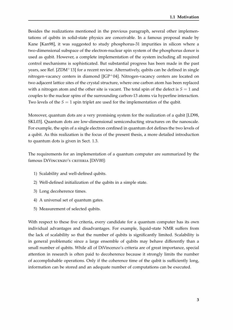
Fig. 1.1: Transmission electron microscopy image of a self-assembled InAs quantum dotgrown in GaAs. The InAs/GaAs layers are embedded in a heterostructure to enable thecontrol of the electronic population of the dot. Figure is taken from Ref. [War13].
1.3 Quantum dots
Quantum dots are small three dimensional structures on the nanoscale which are confined
in all three spatial dimensions. Due to the confinement, the energy levels of an electron or
a hole placed inside the dot are discrete, similar to a particle in a box or to the electronic
levels of an atom. Thus, quantum dots are often referred as “artificial atoms”. Besides their
importance for QIP, quantum dots also play a big role in the field of spintronics [ŽFDS04].
In the following, we briefly present two different types of quantum dots relevant for QIP.
Self-assembled quantum dots grow randomly on a substrate [War13]. In Fig. 1.1, the trans-
mission electron microscopy image of a typical InAs quantum dot embedded in GaAs
is shown. Layer-by-layer, InAs is grown on the GaAs substrate. Thereby, InAs quantum
dots form randomly which are capped by additional GaAs layers. To control the electronic
occupation of the dot, they are integrated into an additional heterostructure to enable a
tuning of the electronic levels by a gate voltage. The size of such a self-assembled quantum
dot lies typically in the order of magnitude of ten nanometers. Due to its potential depth, a
self-assembled quantum dot can be operated at fairly high temperatures T & 4 K. The elec-
tron spin is controlled optically. The required laser pulses do not exceed a few picoseconds
and enable ultrafast rotations of the spins with a high fidelity [GES+09, War13]. Measure-
ments are usually performed on an ensemble of randomly located quantum dots. Pump
and probe spectroscopy revealed that the ensemble dephasing time T∗2 does not exceed a
few nanoseconds [GYS+06, HGB+08]. But the dephasing time T2 of a single dot lies in the
scale of microseconds for temperatures T < 15-20 K. The longitudinal relaxation time T1
is much longer than the dephasing time T2. At T = 1 K, it reaches values of T1 ≈ 20 ms
as long as the magnetic field is not too large [KDH+04]. The properties of self-assembled
6
1.3 Quantum dots
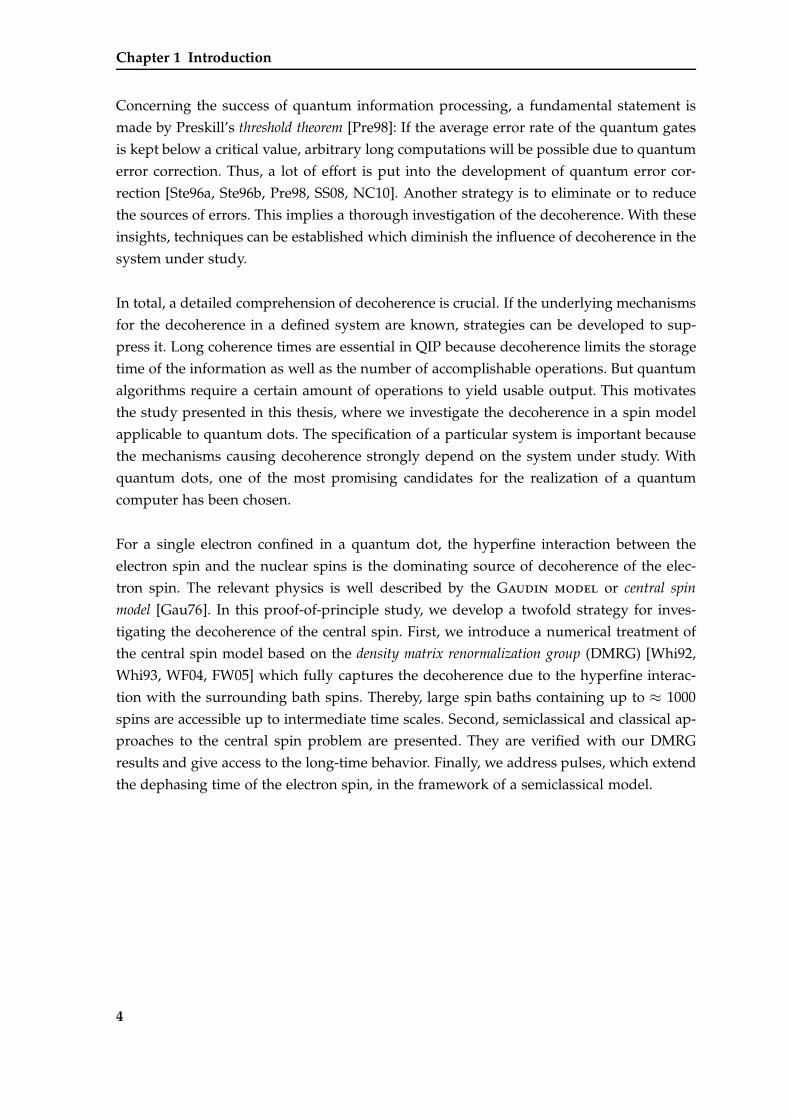
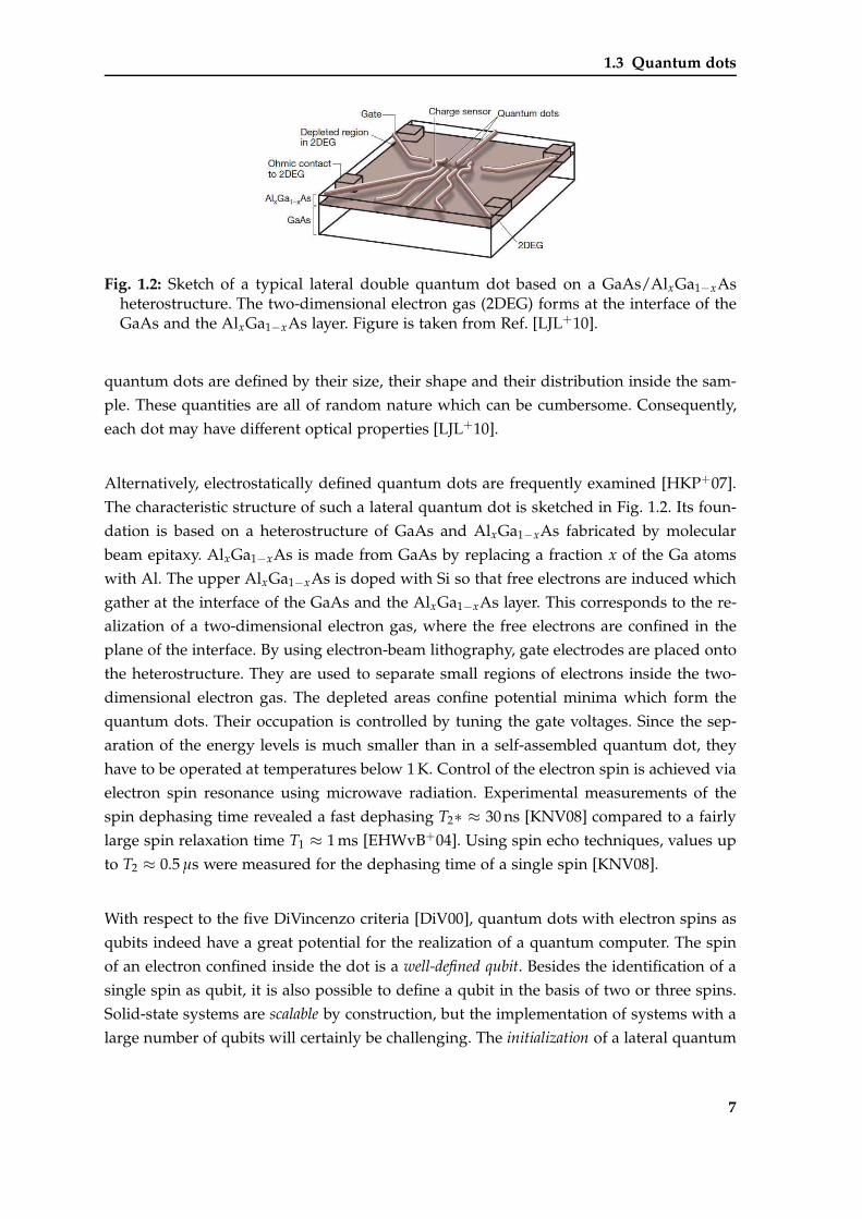
Fig. 1.2: Sketch of a typical lateral double quantum dot based on a GaAs/AlxGa1−xAsheterostructure. The two-dimensional electron gas (2DEG) forms at the interface of theGaAs and the AlxGa1−xAs layer. Figure is taken from Ref. [LJL+10].
quantum dots are defined by their size, their shape and their distribution inside the sam-
ple. These quantities are all of random nature which can be cumbersome. Consequently,
each dot may have different optical properties [LJL+10].
Alternatively, electrostatically defined quantum dots are frequently examined [HKP+07].
The characteristic structure of such a lateral quantum dot is sketched in Fig. 1.2. Its foun-
dation is based on a heterostructure of GaAs and AlxGa1−xAs fabricated by molecular
beam epitaxy. AlxGa1−xAs is made from GaAs by replacing a fraction x of the Ga atoms
with Al. The upper AlxGa1−xAs is doped with Si so that free electrons are induced which
gather at the interface of the GaAs and the AlxGa1−xAs layer. This corresponds to the re-
alization of a two-dimensional electron gas, where the free electrons are confined in the
plane of the interface. By using electron-beam lithography, gate electrodes are placed onto
the heterostructure. They are used to separate small regions of electrons inside the two-
dimensional electron gas. The depleted areas confine potential minima which form the
quantum dots. Their occupation is controlled by tuning the gate voltages. Since the sep-
aration of the energy levels is much smaller than in a self-assembled quantum dot, they
have to be operated at temperatures below 1 K. Control of the electron spin is achieved via
electron spin resonance using microwave radiation. Experimental measurements of the
spin dephasing time revealed a fast dephasing T2∗ ≈ 30 ns [KNV08] compared to a fairly
large spin relaxation time T1 ≈ 1 ms [EHWvB+04]. Using spin echo techniques, values up
to T2 ≈ 0.5 µs were measured for the dephasing time of a single spin [KNV08].
With respect to the five DiVincenzo criteria [DiV00], quantum dots with electron spins as
qubits indeed have a great potential for the realization of a quantum computer. The spin
of an electron confined inside the dot is a well-defined qubit. Besides the identification of a
single spin as qubit, it is also possible to define a qubit in the basis of two or three spins.
Solid-state systems are scalable by construction, but the implementation of systems with a
large number of qubits will certainly be challenging. The initialization of a lateral quantum
7
Chapter 1 Introduction
dot is achievable by relaxation or by populating the dots with selected spin states, which
can be realized by adjusting the coupling to the reservoir [HKP+07]. For self-assembled
quantum dots, reliable initialization is achieved by optical pumping [War13]. Both single
lateral as well as single self-assembled quantum dots have relatively long decoherence times.
By applying schemes from dynamic decoupling [Ban98, VL98, KL05, Uhr07, Lev08], the
decoherence time can be increased further. In addition, the optical control of a single
spin in a self-assembled quantum dot is very fast so that a large number of operations
can be performed. For computations, a universal set of quantum gates is required which is
represented by a single-qubit and a two-qubit gate [LD98]. A single-qubit gate corresponds
to a rotation of the spin. As an example for the required two-qubit gate, one may consider
the SWAP gate which exchanges the state of two spins. For a detailed review of possible
realizations, see Ref. [LYS10] for self-assembled and Ref. [HKP+07] for lateral quantum
dots. In combination, the single-qubit and the two-qubit gate can be used to implement
arbitrary quantum gates. The measurement of qubits in lateral quantum dots is based on
the conversion of the spin state to a charge state. The detection of a single charge is much
easier than the measurement of a tiny magnetic moment so that this technique is the
method of choice. For the spin-to-charge conversion, a variety of different methods has
been proposed [HKP+07]. Spontaneous emission and Faraday rotation enable the optical
measurement of spins in self-assembled quantum dots, see Ref. [War13] for a summary.
In total, the realization of a quantum computer with electron spins in quantum dots com-
plies with DiVincenzo’s criteria [DiV00] in many aspects. In the future, the experimental
as well as the theoretical progress will certainly improve the situation further.
Alternatively, qubits in quantum dots are also realizable via excited electron-hole pairs
(excitons) which are created with short laser pulses. For example, by creating a single
exciton in two quantum dots, the basis states are used to define two qubits [BHH+01].
Furthermore, qubits can also be represented by hole spins [War13]. This is an independent
and currently very active field in research.
In this theses, we discuss the realization of qubits in the two-levels of a single electron spin
confined in a quantum dot. Hence, a qubit is always identified with an electron spin-1/2
and vice versa from now on. As mentioned above, the decoherence of the electron spin
is an important issue in QIP. In the next sections, we discuss the underlying mechanisms
and introduce an appropriate model.
8
1.3 Quantum dots
1.3.1 Decoherence of an electron spin in a quantum dot
The dominating source for the decoherence of electron spins in solids is usually based on
spin-orbit coupling. By spin-orbit interaction, the spin couples to the electronic degrees
of freedom which are exposed to various perturbing effects such as impurity scattering
or electron-phonon interaction. However, an analysis of the spin-flip rates [KN00, KN01]
revealed that the relaxation of the electron spin due to spin-orbit coupling with electron-
phonon coupling is strongly suppressed for electrons confined in an s-type conduction
band of a quantum dot. In a consecutive investigation, the dephasing of the electron
spin [GKL04] was included in the analysis of the spin-orbit interaction. Based on pertur-
bation theory and a Markovian approximation, it was found that the transverse relaxation
time T2 exceeds the longitudinal relaxation time T1 with T2 = 2T1. This result is general
and does not depend on the nature of the fluctuations coupling to the orbital degrees
of freedom. Hence, if spin orbit coupling alone was the dominating mechanism for the
decoherence, a single electron spin confined in a quantum dot would exhibit very long
dephasing times because T1 ≈ 1-20 ms, see previous section.
However, experimental observations contradict with this theoretical result. Measurements
revealed strongly reduced dephasing times compared to to relaxation time, see previous
section. Thus, spin-orbit coupling alone cannot be the major source of decoherence. In-
stead, the decoherence is dominated by the Fermi contact hyperfine interaction between
the electron spin and the nuclear spins in the dot. This is supported by the fact that com-
mon semiconducting materials such as GaAs or InAs have a substantial nuclear magnetic
moment of the order of several nuclear magnetons [SKL03]. This is comparable to the sce-
nario in single nitrogen-vacancy centers, where the hyperfine interaction between the spin
of the nitrogen-vacancy center and the nuclear spins of the surrounding carbon-13 atoms
is the dominating contribution to decoherence.
According to Fermi [Fer30], the hyperfine interaction is proportional to the probability
|Ψ(~rj)|2 that the electron is at the site~rj of the nucleus. For a single nucleus, the Hamilto-
nian of the hyperfine interaction between the electron spin ~S0 and a single nuclear spin ~Ii
is given by the expression [MER02, SKL03, CL06]
Hi = Ji~S0 ·~Ii. (1.1)
The coupling constant reads
Ji =6π
3IµBµIi
∣∣Ψ(~ri)∣∣2 , (1.2)
9
Chapter 1 Introduction
where µB stands for the Bohr magneton of the electron and µIifor the magneton of the
nucleus i. We assume that the electron is in its orbital ground state so that the hyperfine
exchange can be regarded as isotropic. Placed inside a quantum dot, the electron spin
interacts with about N = 106 nuclear spins [SKL03]. The sign of the interaction depends
on the compound, for instance, it is antiferromagnetic for GaAs and InAs. The time scale
for the decoherence of the electron spin is set by the total contribution Jq of all nuclear
spins with J2q ∼ ∑
Ni=1 |Ψ(~ri)|4 [MER02].
In addition to the hyperfine coupling, the nuclear spins interact with one another by
dipole-dipole exchange. For two nuclear spins i and j, the dipolar interaction is described
by the Hamiltonian [SKL03]
Hij = − µ2I
Ii Ij
1r3
ij
3(~Ii~rij
) (~Ij~rij
)
r2ij
−~Ii ·~Ij
, (1.3)
where ~rij is the spatial distance between the nuclei. The time scale of the hyperfine in-
teraction is of the order 10−6 s, while the dipolar coupling affects the decoherence of the
electron spin on a time scale which is roughly one or two orders of magnitudes larger. This
time scale lies beyond the scope of the present thesis. Consequently, we will not consider
the dipolar coupling further.
1.4 Central spin model
The previously introduced hyperfine interaction between a single electron spin and a bath
of surrounding nuclear spins in a quantum dot is well captured by the central spin or
Gaudin model [Gau76, Gau83]
H = ~S0
N
∑i=1
Ji~Si
=N
∑i=1
Ji
[Sz
0Szi +
12
(S+
0 S−i + h.c.
)].
(1.4)
The term Gaudin model refers originally to a class of integrable spin models first proposed
by Gaudin in 1976 [Gau76]. This family of models is closely related to the pairing-model
in the BCS theory of superconductivity, see for instance Ref. [vDP02] or the review in
Ref. [DPS04] and the references therein.
10
1.4 Central spin model
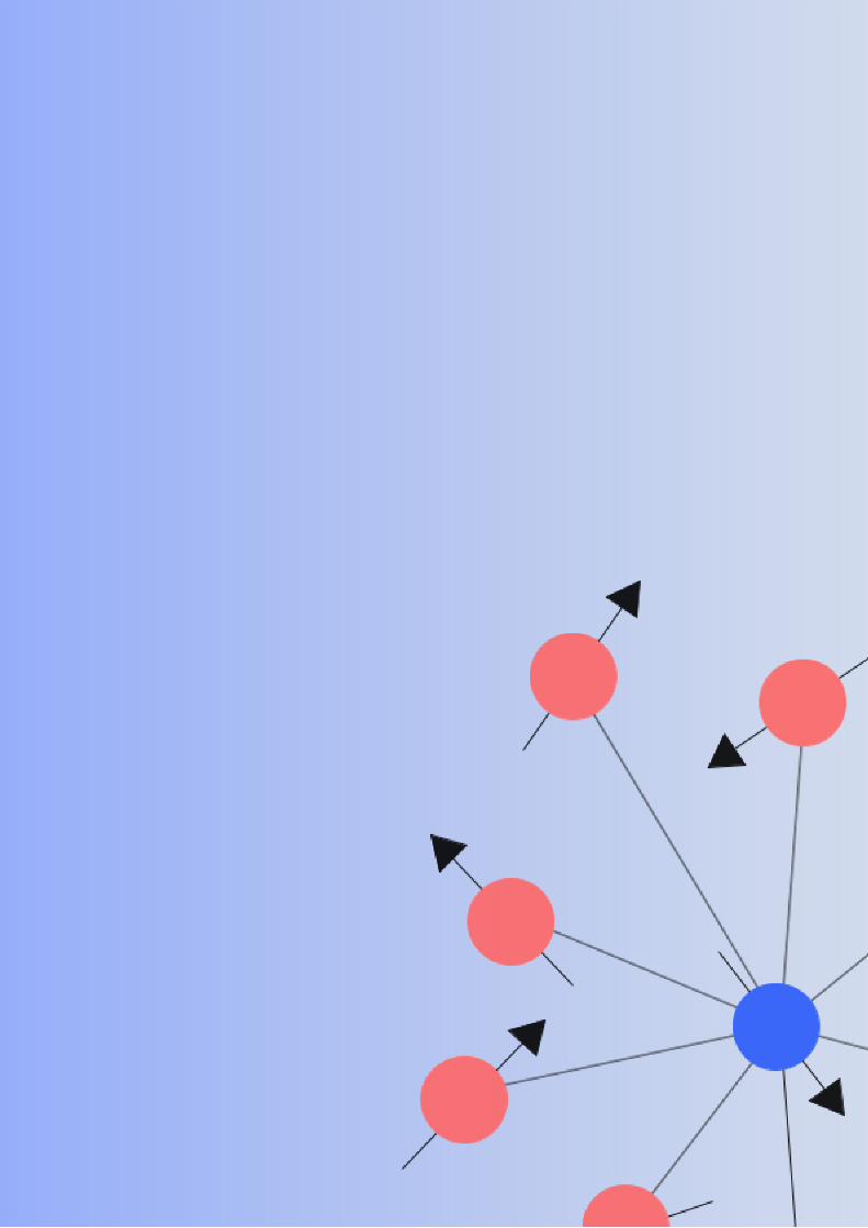
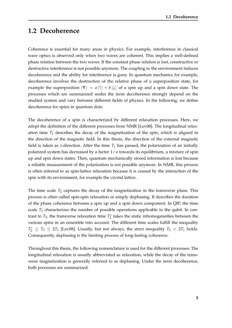
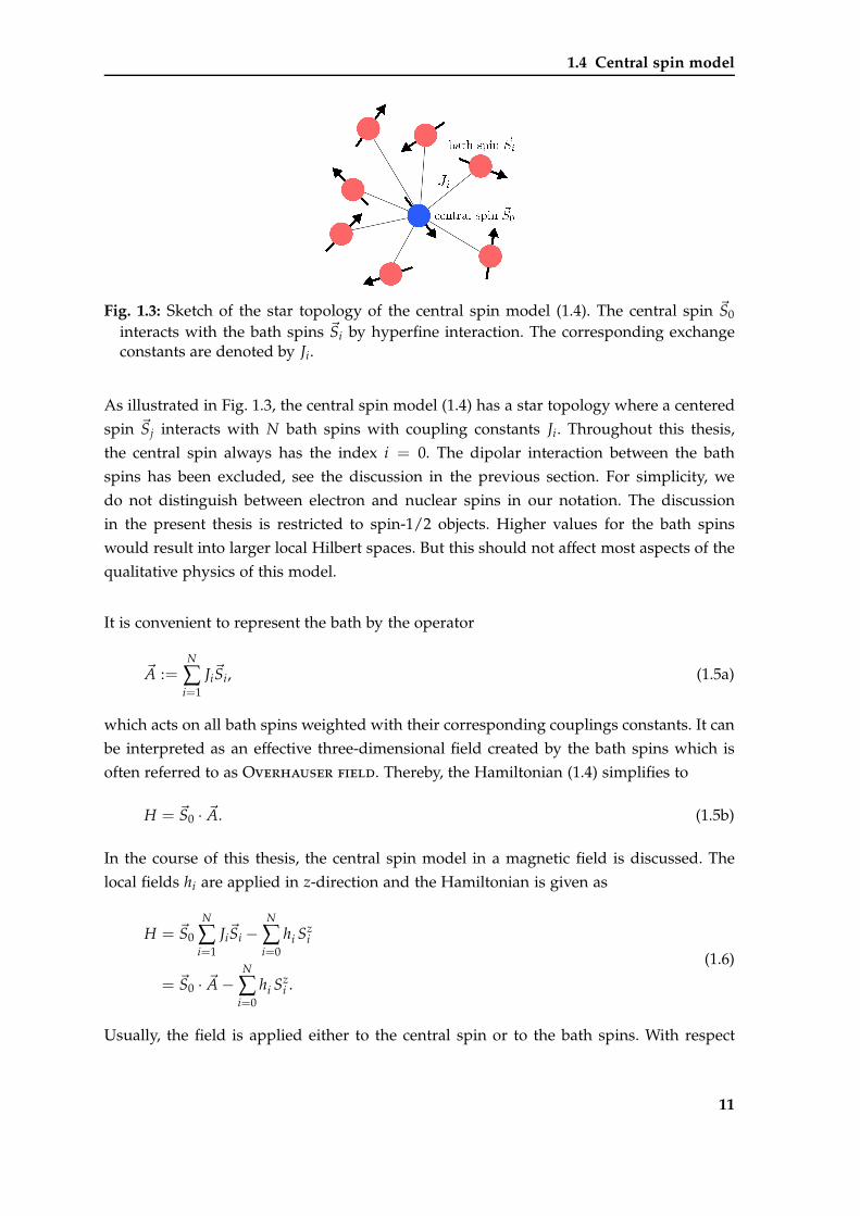
Fig. 1.3: Sketch of the star topology of the central spin model (1.4). The central spin ~S0
interacts with the bath spins ~Si by hyperfine interaction. The corresponding exchangeconstants are denoted by Ji.
As illustrated in Fig. 1.3, the central spin model (1.4) has a star topology where a centered
spin ~Sj interacts with N bath spins with coupling constants Ji. Throughout this thesis,
the central spin always has the index i = 0. The dipolar interaction between the bath
spins has been excluded, see the discussion in the previous section. For simplicity, we
do not distinguish between electron and nuclear spins in our notation. The discussion
in the present thesis is restricted to spin-1/2 objects. Higher values for the bath spins
would result into larger local Hilbert spaces. But this should not affect most aspects of the
qualitative physics of this model.
It is convenient to represent the bath by the operator
~A :=N
∑i=1
Ji~Si, (1.5a)
which acts on all bath spins weighted with their corresponding couplings constants. It can
be interpreted as an effective three-dimensional field created by the bath spins which is
often referred to as Overhauser field. Thereby, the Hamiltonian (1.4) simplifies to
H = ~S0 · ~A. (1.5b)
In the course of this thesis, the central spin model in a magnetic field is discussed. The
local fields hi are applied in z-direction and the Hamiltonian is given as
H = ~S0
N
∑i=1
Ji~Si −
N
∑i=0
hi Szi
= ~S0 · ~A −N
∑i=0
hi Szi .
(1.6)
Usually, the field is applied either to the central spin or to the bath spins. With respect
11
Chapter 1 Introduction
to nuclear spins, magnetic fields are often neglected because the Zeeman splitting is very
small due to the small magnetic moments of the nuclei. In contrast, the Bohr magneton
of the electron is about three orders of magnitude larger. But fields applied to bath spins
induce a dynamics in the bath which is exploited in the course of this thesis as simple
example of an intrinsic bath dynamics.
The coupling constants Ji are inhomogeneous because they are defined by the probability
|Ψ(~ri)|2 that the electron is present at the site of the nucleus i. As mentioned before, the
time scale for the decoherence is defined by the total contribution of all nuclear spins. In
the present thesis, we focus mainly on a completely disordered initial state where the first
moment of the coupling constants does not contribute. Hence, it is advisable to define
the time scale for the fast dynamics as 1/Jq where J2q is given by the quadratic sum of all
couplings [MER02]
J2q :=
N
∑i=1
J2i . (1.7)
Note that we use units where h = 1 so that Jq corresponds to an energy. The Ji are dis-
tributed randomly, since the nuclear spins are located randomly inside the dot. By em-
ploying experimentally measured values and an approximation for the wave function, it
is possible to model the distribution of the exchange constants inside a spherical quantum
dot, see for instance Ref. [SKL03].
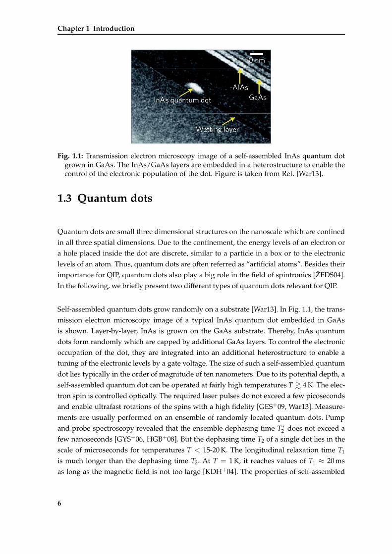
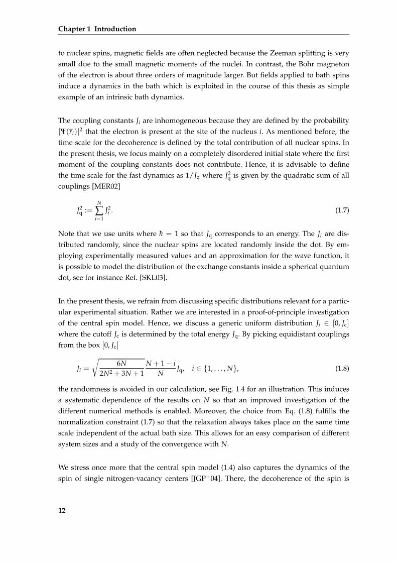
In the present thesis, we refrain from discussing specific distributions relevant for a partic-
ular experimental situation. Rather we are interested in a proof-of-principle investigation
of the central spin model. Hence, we discuss a generic uniform distribution Ji ∈ [0, Jc]
where the cutoff Jc is determined by the total energy Jq. By picking equidistant couplings
from the box [0, Jc]
Ji =
√6N
2N2 + 3N + 1N + 1 − i
NJq, i ∈ 1, . . . , N, (1.8)
the randomness is avoided in our calculation, see Fig. 1.4 for an illustration. This induces
a systematic dependence of the results on N so that an improved investigation of the
different numerical methods is enabled. Moreover, the choice from Eq. (1.8) fulfills the
normalization constraint (1.7) so that the relaxation always takes place on the same time
scale independent of the actual bath size. This allows for an easy comparison of different
system sizes and a study of the convergence with N.
We stress once more that the central spin model (1.4) also captures the dynamics of the
spin of single nitrogen-vacancy centers [JGP+04]. There, the decoherence of the spin is
12
1.5 Overview of methods
Fig. 1.4: Uniform probability distribution p(J) of the coupling constants J ∈ [0, Jc]. To avoidthe randomness in our calculation, we pick equidistant couplings Ji from the box [0, Jc]for i = 1, . . . , N, see Eq. (1.8).
dominated by the hyperfine interaction with the non-vanishing nuclear magnetic moment
of the carbon-13 atoms. However, a corresponding theoretical study comprises a significant
dipole-dipole interaction which induces stronger fluctuations in the bath [MTL08].
1.5 Overview of methods
First investigations of the central spin model (1.4) in the 1970s were based on the Bethe
ansatz [Gau76, Gau83]. Over the years, the model has become very popular for the de-
scription of the hyperfine interaction of an electron spin in a quantum dot. Nowadays,
the central spin model has been studied in the framework of many different methods. Be-
sides standard techniques such as exact diagonalization, more elaborate methods such
as cluster expansion [WdSDS05] or non-Markovian master equation formalism [CL04] have
been applied to the model. These techniques give access to larger bath sizes, but of-
ten require additional approximations which limit the universality of the results. For
example, many applications are restricted to the strong-field limit where spin-flips be-
tween the central spin and the bath can be neglected or treated perturbatively. For the
sake of completeness, we also mention perturbative [KLG02, KLG03] and Markovian ap-
proaches [SMP02, dSDS03a, dSDS03b].
In practice, the method should be chosen with respect to the aim of study. For a full study
of the decoherence the time evolution of the observables has to be calculated for a sizeable
nuclear bath over a large period of time. In exact diagonalization, the reachable time scale
is only limited by CPU time. However, only small systems with N ≈ 20 bath sites can
be implemented [SKL03, CDDS10]. Within the available amount of CPU resources, the
accessible time scale is extended further by calculating the time evolution in the framework
of Chebychev polynomials [DDR03, HA14].
13
Chapter 1 Introduction
Our study is based on the density matrix renormalization group (DMRG) [Whi92, Sch05a],
which is introduced in the next chapter. There, we also present several extensions to time-
dependent DMRG (tDMRG) [WF04, FW05, Sch05a]. The numerical treatment within the
framework of tDMRG fully captures the hyperfine exchange between the central spin and
the bath. Compared to exact diagonalization, the number of accessible bath spins is larger
by up to two orders of magnitude, but the reachable time scales are more limited. In
addition, a semiclassical and a classical model for the decoherence is introduced in the
progress of this thesis. Both approaches can be combined to justify an effective description
of the electron spin dynamics.
In this section, we briefly introduce a selection of different methods and describe their
potential and limits. This short review does not claim to be complete; its purpose is to give
a first impression of different treatments of the central spin model.
1.5.1 Bethe ansatz
The central spin model (1.4) is exactly solvable by Bethe ansatz [Gau76, Gau83]. However,
finding the solutions is highly non-trivial and strongly depends on the initial state of the
system. The Bethe ansatz gives access to the eigen decomposition of the Hamiltonian.
To this end, the Bethe ansatz equations have to be solved. For the central spin model,
the number of equations corresponds to the number M of flipped spins, starting from
an entirely polarized state. In total, there are CNM different solutions, called Bethe roots,
of the coupled Bethe ansatz equations where CNM stands for the binomial coefficient. The
Bethe roots correspond to a complete representation of the eigenvalues and -vectors of the
Hamiltonian. They are used to calculate the time dependence of the desired observables,
for example the magnetization of the central spin.
As mentioned before, solving the Bethe ansatz is a highly complicated task. Thus, the
solutions are usually restricted to initial states where the bath is either fully polarized or
where only a small number of spins is flipped [BS07b, BS07a]. Especially the calculation
of observables is costly because it requires the summation of CNM terms. However, it was
demonstrated that the Bethe ansatz can be used to extract important features, for example
the dominating frequencies in the spectral representation of the magnetization without
summing over a very large number of contributions [BES+10a]. Thereby, an estimate for
the longitudinal relaxation time T1 of the electron can be made. The results are valid even
for low polarizations of the bath, depending on the exact properties of the distribution of
the exchange constants. Furthermore, the Bethe ansatz was employed for a calculation of
14
1.5 Overview of methods
the static magnetization profile and the static two-point correlation function of the central
spin model [BES10b]. The corresponding Bethe ansatz result was combined with a classical
approximation and exact diagonalization results. While the magnetization profile of the
classical approximation is close to the one of the quantum mechanical model, the two-
point correlation function shows significant contributions from quantum fluctuations.
Recently, a method combining the algebraic Bethe ansatz and Monte Carlo sampling was
proposed [FS13a, FS13b]. In this variant, a restriction to a definite polarization of the bath
is not necessary. So far, the real-time evolution of up to N = 48 spins was calculated up to
long times t ≈ 100-1000 J−1q . As there is no restriction to states with a certain polarization,
the calculation in combination with the Monte Carlo sampling approximates the complete
trace in the Hilbert space. However, this approach can be applied only if the coupling
constants are isotropic. In contrast, the XXZ version of the central spin model, where the
coupling constants in z-direction differ from the ones in the xy-plane, may be investigated
with the DMRG.
1.5.2 Cluster expansion techniques
Cluster expansions are used to study models which describe the decoherence due to spec-
tral diffusion. Spectral diffusion implies that a dipolar interaction between the bath spins
is the dominant mechanism for the decoherence of the central spin. In addition, a secular
approximation is usually made. This corresponds to the neglection of spin-flips between
the central spin and the bath. The approximation is justified in the strong-field limit rele-
vant for many experimental studies. Consequently, only the transverse relaxation time T2
can be studied within this approach. A longitudinal relaxation does not take place within
this approximation.
For the cluster expansion developed by Witzel et al. [WdSDS05, WDS06], the fluctuations
of the bath are approximated by sub-processes. To this end, the bath is separated into
small disjoint clusters. The lowest order is given by all processes including two nuclear
spins, because a single nuclear spin has no contribution. The number of involved spins
is successively increased. Thus, contributions from clusters with three nuclear spins are
taken into account followed by contributions from four nuclei which cannot be represented
by sub-processes caused by the interaction of two nuclear spins. Consequently, the n-th
order of the cluster expansion contains contributions of all clusters consisting of up to n
spins. To obtain a result, the desired quantity has to be expanded in terms of the cluster
contributions. Then, the individually calculated cluster contributions up to a certain order
15
Chapter 1 Introduction
are inserted to evaluate the expression. Convergence is achieved when the contribution of
the clusters decreases quickly with their size. This is supported by the fact that the dipolar
interaction between two randomly located nuclear spins with distance R decays extremely
fast ∼ 1/R3. Hence, the contribution of spins with a large spatial distance only plays a
minor role in the total contribution, while a contribution of neighbored spins is crucial.
Besides the technique sketched above, other variants of cluster expansions exist. Based on
the original scheme [WdSDS05, WDS06], the disjoint cluster approach was introduced and
applied to nitrogen-vacancy centers in diamond [MTL08]. The correlated cluster expansion
developed by Yang and Liu [YL08a, YL09] is extremely suitable when contributions from
larger clusters have to be taken into account. It has been applied successfully to study
pulse sequences which extend the coherence time of the electron spin [DRZ+09, ZWL11,
ZHL12].
The main disadvantage of the cluster expansion techniques is the restriction to pure de-
phasing of the central spin. A modified version of the correlated cluster expansion in-
cludes spin-flips between central spin and bath on the level of a one-cluster contribu-
tion [WCCDS12], but the results are restricted to small time scales. Moreover, a very large
number of clusters has to be taken into account when the size of the bath is large.
1.5.3 Non-Markovian master equation formalism
The decoherence of the electron spin in the central spin model shows strongly non-
Markovian behavior [BBP04, CL04]. This is also underlined by the fact that the bath in the
central spin model has no intrinsic dynamics. Hence, a derivation of the equations of mo-
tion based on a Markovian approximation is generally insufficient, see Sect. 1.5.5. The lack
of non-Markovian contributions can be repaired by considering the application of non-
Markovian master equations. Here, we follow the notation used in Refs. [BP07, FB07].
The non-Markovian master equation formalism is based on the Liouville or von Neumann
equation of the density matrix. The density matrix ρ of the total system is projected onto
the so-called “relevant part” Pρ by the application of a projection operator P . The projec-
tion operator P is chosen in a way that all irrelevant degrees of freedom are eliminated.
A generic choice for the relevant part is Pρ = TrE(ρ)⊗ ρ0, where the partial trace is taken
over the Hilbert space of the environment, for example the bath, with the fixed state ρ0
of the environment. The remaining part of the Hilbert space is called the system. With
16
1.5 Overview of methods
the superoperator P satisfying the condition Pρ(0) = ρ(0), one derives the Nakajima-
Zwanzig equation
ddt
Pρ (t) =
t∫
0
dt1 K (t, t1)Pρ (t1) (1.9)
for the reduced density matrix where the so-called memory Kernel or self-energy K(t, t1)
induces the non-Markovian behavior. The Nakajima-Zwanzig equation is an integrodiffer-
ential equation for the effective dynamics of the quantum mechanical system defined by
the “relevant part”. In general, the obtained master equation cannot be solved in closed
form. To this end, it is usually simplified further by applying additional approximations
and a perturbative expansion of the kernel in powers of the interaction between the system
and the bath. In the final step, the simplified master equation is often solved analytically.
Alternatively, the time-convolutioness master equation
ddt
Pρ (t) = K (t)Pρ (t) (1.10)
can be solved. It is also derived from the von Neumann equation. Compared to the
Nakajima-Zwanzig equation, the dependence on the history of the relevant part has been
eliminated by the employment of an exact backward propagator [BP07]. Thus, the time-
convolutioness master equation is a time-local equation which is often preferred to the
time-convolution in the Nakajima-Zwanzig equation. The superoperator K(t) is a time-
dependent generator which introduces the non-Markovian behavior. Like the self-energy
in Eq. (1.9), the generator K(t) is usually derived from a perturbative expansion in the
interaction between system and bath.
In one of the first studies, a generalized master equation was derived by defining a su-
peroperator which preserved all electron spin excitations [CL04]. Thereby, the solution for
the relaxation and dephasing of the electron spin due to hyperfine coupling was found
in the strong-field limit. In the zero-field limit, only a lower bound for the decaying frac-
tion of the electron spin could be estimated. By comparing solutions from non-Markovian
master equations with the exact result for the reduced dynamic of the electron spin in
the central spin model with XX interaction, Breuer et al. [BBP04] demonstrated that both
the Nakajima-Zwanzig as well as time-convolutioness master equation yield a good ap-
proximation for the short-time behavior. However, the approach failed for larger times
where partially unphysical behavior occurred. The standard projection operator as in-
troduced above reduces the total state to a tensor product state between system and
bath. An advanced approach is based on correlated projection operators which partly
preserve the correlation between system and bath [FB07]. The results were compared
17
Chapter 1 Introduction
to the exact solution of the central spin model with homogeneous coupling constants.
Even in lowest order, a nice agreement between all results was found. For the model
with non-uniform exchange constants, the same conclusion was reached for the short-
and long-time behavior in the high-field limit [FBN+08]. The study was based on the
time-convolutioness master equation and correlated projection operators. In a more recent
publication, a non-perturbative solution of the time-convolutioness master equation was
presented by Barnes et al. [BCDS12]. After a resummation of all orders of the master equa-
tion, the solution can be written in a closed form. It is valid for inhomgeneous couplings as
well as for a large number of different initial states. However, this calculation still requires
a finite magnetic field and is restricted to a small time-scale defined by the inverse of the
largest coupling constant.
In all, the non-Markovian master equation formalism captures the decoherence of the elec-
tron spin in the central spin model for finite magnetic fields on limited time-scales. Solu-
tions for the long-time behavior are restricted to the strong-field regime. Furthermore, the
employment of non-Markovian master equations provides access to an analytical treat-
ment of the model. But master equations involve many approximations and the output
depends on the assumptions made during their derivation .
1.5.4 Semiclassical and classical approaches
Semiclassical and classical models for the decoherence of an electron spin are frequently
studied. The spins of the bath and/or the central spin are approximated either by classical
spins or by an effective field. Note that the dynamics of classical spins is closely related to
the one of quantum spins due to the isomorphism between the rotation group SO(3) and
the group SU(2) of complex rotations.
Merkulov et al. [MER02] studied the hyperfine-induced decoherence of electron spins in a
large ensemble of quantum dots without magnetic field and in the strong-field limit. Three
different processes were identified which contribute to the decoherence of the electron
spin with different impact. First, the electron spin precesses in the frozen hyperfine field
of the nuclear spins. Second, fluctuations in the hyperfine field of the nuclear spins were
discussed. They are induced by the precession of the nuclear spins in the hyperfine field
of the electron, which is smaller by the factor 1/√
N than the field acting on the electron
spin. A third time scale is set by the dipolar coupling between the nuclear spins. But this
effect was not included since many other mechanisms contribute to the decoherence on
the long-time scale of the dipolar interaction. All equations of motion were treated on a
classical level and estimates for the spin dephasing time T∗2 were calculated.
18
1.5 Overview of methods
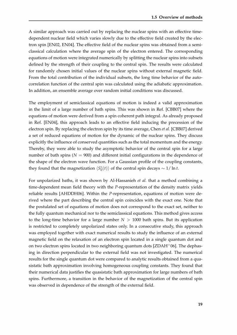
A similar approach was carried out by replacing the nuclear spins with an effective time-
dependent nuclear field which varies slowly due to the effective field created by the elec-
tron spin [EN02, EN04]. The effective field of the nuclear spins was obtained from a semi-
classical calculation where the average spin of the electron entered. The corresponding
equations of motion were integrated numerically by splitting the nuclear spins into subsets
defined by the strength of their coupling to the central spin. The results were calculated
for randomly chosen initial values of the nuclear spins without external magnetic field.
From the total contribution of the individual subsets, the long time behavior of the auto-
correlation function of the central spin was calculated using the adiabatic approximation.
In addition, an ensemble average over random initial conditions was discussed.
The employment of semiclassical equations of motion is indeed a valid approximation
in the limit of a large number of bath spins. This was shown in Ref. [CBB07] where the
equations of motion were derived from a spin coherent path integral. As already proposed
in Ref. [EN04], this approach leads to an effective field inducing the precession of the
electron spin. By replacing the electron spin by its time average, Chen et al. [CBB07] derived
a set of reduced equations of motion for the dynamic of the nuclear spins. They discuss
explicitly the influence of conserved quantities such as the total momentum and the energy.
Thereby, they were able to study the asymptotic behavior of the central spin for a large
number of bath spins (N = 900) and different initial configurations in the dependence of
the shape of the electron wave function. For a Gaussian profile of the coupling constants,
they found that the magnetization 〈Sz0(t)〉 of the central spin decays ∼ 1/ ln t.
For unpolarized baths, it was shown by Al-Hassanieh et al. that a method combining a
time-dependent mean field theory with the P-representation of the density matrix yields
reliable results [AHDDH06]. Within the P-representation, equations of motion were de-
rived where the part describing the central spin coincides with the exact one. Note that
the postulated set of equations of motion does not correspond to the exact set, neither to
the fully quantum mechanical nor to the semiclassical equations. This method gives access
to the long-time behavior for a large number N > 1000 bath spins. But its application
is restricted to completely unpolarized states only. In a consecutive study, this approach
was employed together with exact numerical results to study the influence of an external
magnetic field on the relaxation of an electron spin located in a single quantum dot and
on two electron spins located in two neighboring quantum dots [ZDAH+06]. The dephas-
ing in direction perpendicular to the external field was not investigated. The numerical
results for the single quantum dot were compared to analytic results obtained from a qua-
sistatic bath approximation involving homogeneous coupling constants. They found that
their numerical data justifies the quasistatic bath approximation for large numbers of bath
spins. Furthermore, a transition in the behavior of the magnetization of the central spin
was observed in dependence of the strength of the external field.
19
Chapter 1 Introduction
Recently, Witzel et al. [WYD13] introduced a semiclassical description of the spin bath. The
autocorrelation function of the bath fluctuations were obtained from a correlated cluster
expansion using the secular approximation, see Sect. 1.5.2. Hence, the model only com-
prises dephasing due to spectral diffusion. The relaxation of the electron spin was not
included. The exclusion of back-action effects between central spin and bath is legitimated
by their model, which contains an intrinsic dynamics of the bath. However, this is generally
not justified for the central spin model where the bath has no intrinsic dynamics.
1.5.5 Other approaches
A perturbative ansatz can be made in the spin-flip terms of the Hamiltonian of the central
spin model (1.4). This ansatz is only justified in the limit of strong magnetic fields. Oth-
erwise it cannot be guaranteed that the contribution from the spin-flips is small. Indeed,
a comparison with an exact solution lead to the conclusion that the perturbative treat-
ment yields a different behavior in the zero-field limit, see Ref. [SKL03] and the references
therein.
Alternatively, it is possible to solve a master equation where the nuclear spin bath is ap-
proximated by a Markovian process among other simplifications [SMP02]. In general, the
dynamics of the nuclear spins in the central spin model is non-Markovian because the
bath has no intrinsic dynamics. The dynamics of the nuclear spins is determined entirely
by the interaction with the central spin. Hence, intrinsic dynamics of the bath are essential
for the Markovian approximation because it is assumed that the bath is independent from
the state of the central spin. Consequently, it is not surprising that the results of this study
stand in contradiction to known results. Furthermore, a Markovian approximation was
also made in the strong-field limit where the decoherence is governed by spectral diffu-
sion [dSDS03a, dSDS03b]. This approach involves many assumptions and approximations
so that the calculated decoherence times exceed the ones measured in experiment.
Other attempts to describe the non-Markovian physics in the central spin model were
made on the level of an iterative equation of motion approach for the retarded Green’s
function of the electron spin in the large-bath limit [DH06, DH08]. Thereby, good results
are yield for strong external fields where the contribution of higher orders is negligible.
20
1.6 Pulses & dynamic decoupling
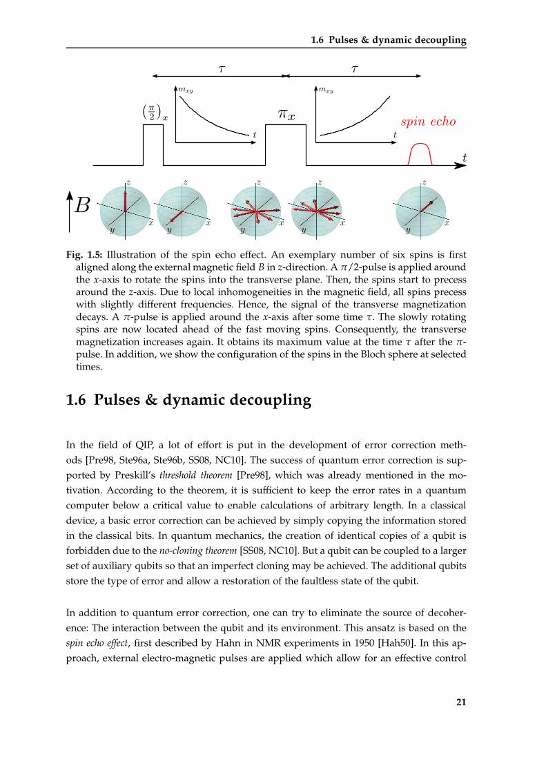
Fig. 1.5: Illustration of the spin echo effect. An exemplary number of six spins is firstaligned along the external magnetic field B in z-direction. A π/2-pulse is applied aroundthe x-axis to rotate the spins into the transverse plane. Then, the spins start to precessaround the z-axis. Due to local inhomogeneities in the magnetic field, all spins precesswith slightly different frequencies. Hence, the signal of the transverse magnetizationdecays. A π-pulse is applied around the x-axis after some time τ. The slowly rotatingspins are now located ahead of the fast moving spins. Consequently, the transversemagnetization increases again. It obtains its maximum value at the time τ after the π-pulse. In addition, we show the configuration of the spins in the Bloch sphere at selectedtimes.
1.6 Pulses & dynamic decoupling
In the field of QIP, a lot of effort is put in the development of error correction meth-
ods [Pre98, Ste96a, Ste96b, SS08, NC10]. The success of quantum error correction is sup-
ported by Preskill’s threshold theorem [Pre98], which was already mentioned in the mo-
tivation. According to the theorem, it is sufficient to keep the error rates in a quantum
computer below a critical value to enable calculations of arbitrary length. In a classical
device, a basic error correction can be achieved by simply copying the information stored
in the classical bits. In quantum mechanics, the creation of identical copies of a qubit is
forbidden due to the no-cloning theorem [SS08, NC10]. But a qubit can be coupled to a larger
set of auxiliary qubits so that an imperfect cloning may be achieved. The additional qubits
store the type of error and allow a restoration of the faultless state of the qubit.
In addition to quantum error correction, one can try to eliminate the source of decoher-
ence: The interaction between the qubit and its environment. This ansatz is based on the
spin echo effect, first described by Hahn in NMR experiments in 1950 [Hah50]. In this ap-
proach, external electro-magnetic pulses are applied which allow for an effective control
21
Chapter 1 Introduction
of the rotation of the spins. An illustration of the spin echo effect is shown in Fig. 1.5.
An ensemble of spins is initialized in the direction parallel to the external magnetic field.
The spins are rotated into the transverse plane by applying a π/2-pulse around the x- or
y-axis. Due to the Larmor precession, the spins start to rotate in the plane perpendicular
to the external magnetic field. All spins precess with slightly different frequencies because
of inhomogeneities in the local magnetic field. Thus, they dephase with increasing time
and the transverse magnetization decays. By applying a π-pulse after some delay τ, the
situation is inverted: Spins with lower frequencies are now located ahead of the fast rotat-
ing spins. After another delay of length τ, the spins are again in phase and a revival of the
transverse magnetization is observed.
Usually, the inhomogeneities of the local magnetic field are dynamic and not static. This
implies that the application of a single pulse is not anymore sufficient. Instead, the re-
focusing of the spins can be achieved by the implementation of pulse sequences which
are typically iterated. A famous example is the CPMG sequence (Carr, Purcell, Meiboom
and Gill) [CP54, MG58] which consists of two π-pulse cycles. In average, the CPMG se-
quence suppresses the dephasing interaction between the spins and the environment. The
potential power of such sequences is widely known so that the development and opti-
mization of pulse sequences is nowadays a very active field in research. In QIP, pulse se-
quences have been established under the keyword dynamic decoupling (DD) [Ban98, VL98,
FTP+05, KL05, CHHC06, WDS07, YLS07]. While simple DD techniques are also based on
periodic sequences, a breakthrough was achieved by the invention of sequences with non-
equidistant pulses known as Uhrig dynamic decoupling (UDD) [Uhr07]. Thereby, the
decoherence time can be improved by multiple orders for any dephasing system [YL08b].
Furthermore, many other types of DD sequences exist, for example, concatenated dynamic
decoupling [KL05, KL07] or quadratic dynamic decoupling [WFL10]. The first one can be ex-
tended to UDD sequences [Uhr09], while the latter one consists of a combination of two
different UDD sequences. In addition to dephasing, these sequences also suppress the lon-
gitudinal relaxation. This requires that the pulses are quicker than the dynamics of the
environment.
So far, we assumed that the pulses are ideal, which implies infinitesimal duration and
infinite amplitude. In contrast, real pulses always have a finite duration and a finite am-
plitude. The aim is to design real pulses which are as close to an ideal one as possible.
This is achieved by optimizing the time dependence of the pulse amplitudes and of the
rotation axis. In NMR, composite pulses are used to reduce the error due to the finite
pulse duration. In this way, rotations are decomposed in different partial rotations which
are more robust. A theoretical concept for the design of such pulses with piecewise con-
stant amplitudes was first introduced by Tycko [Tyc83]. But the optimization of real pulses
22
1.6 Pulses & dynamic decoupling
can also be carried out for types of pulses other than composite pulses. For example,
pulses with continuous amplitudes or continuous pulses obtained from frequency modu-
lation [SKL+06, PKRU09, FPU12, SFPU12] can be discussed.
A general ansatz for the shaping of pulses is made by a product ansatz for the time-
evolution operator Ure(τp) during a real pulse of duration τp [PKRU09]
Ure
(τp, 0
)= Pτp · Uc
(τp, 0
). (1.11)
The operator Pτp describes the rotation under the ideal pulse, while Uc(τp, 0) is a correct-
ing factor which contains the intrinsic dynamics of the bath (if any) and the interaction
between the spin and the bath. Both operators obey a Schrödinger equation. To make the
real pulse as close as possible to an ideal one, Uc(τp, 0) ≈ 1 has to be fulfilled. Theoreti-
cally, one way to achieve this is to expand the correcting factor in powers of τp so that the
interaction between the spin and the bath is averaged to zero. Precisely, one obtains
Uc
(τp , 0
)= 1+O
(τm+1
p
). (1.12)
We define a pulse with the property (1.12) to be a pulse of order m. Examples for a first or-
der pulse are the symmetric SCORPSE and the asymmetric CORPSE pulses [CJ00, CLJ03].
In the last years, a variety of π and π/2 pulses have been proposed which make corrections
up to second order vanish [SP05, MdSZW06, PQ08, PS08, PKRU09, FPU12, SFPU12].
In ansatz (1.11), a real pulse is compared with an ideal one of infinitesimal length. An
alternative approach is achieved when the dynamics from the pulse and from the system
are disentangled. Then, an optimized pulse of order m has to hold [PFKU08, PU08]
Ure
(τp , 0
)= UH
(τp , τs
)· Pτp
· UH
(τs , 0
)+O
(τm+1
p
), (1.13)
where UH(τ1, τ2) contains the complete time evolution of the system before and after the
pulse and τs denotes the instance of the instantaneous pulse. The advantage of this ansatz
is that both the real as well as the ideal pulse have the same finite duration τp. How-
ever, it was shown that the condition (1.13) can only be fulfilled for a π-pulse in leading
order [PFKU08, PU08]. The vanishing of higher order corrections is excluded rigorously.
In summary, the strategy to suppress the decoherence is twofold:
1) Shape pulses which are as close to an ideal one as possible.
2) Design pulse sequences for dynamic decoupling.
23
Chapter 1 Introduction
A powerful tool for investigating the quality of the analytically derived pulses and pulse
sequences are numerical simulations. They enable an exact study of the specific mod-
els which is only limited by the properties of the employed method and the CPU lim-
its. Furthermore, the higher-order terms in Eq. (1.12) are captured quantitatively. Hence,
a numerical simulation has to be regarded as a complementary method to the analytic
calculations. It quantifies the size of the neglected contributions and is essential for the
verification of the analytically derived pulses and pulse sequences. The quality of shaped
piecewise constant pulses for pure dephasing is discussed on the base of a semiclassical
model in Chapter 5.
24
Chapter 2
Density Matrix Renormalization Group
Contents
2.1 Introduction . . . . . . . . . . . . . . . . . . . . . . . . . . . . . . . . . . . . 26
2.1.1 Reduced density matrix . . . . . . . . . . . . . . . . . . . . . . . . . 29
2.1.2 Truncation of the reduced density matrix . . . . . . . . . . . . . . . 30
2.2 Adaption of DMRG for the central spin model . . . . . . . . . . . . . . . 37
2.2.1 Infinite size algorithm . . . . . . . . . . . . . . . . . . . . . . . . . . 39
2.2.2 Finite size algorithm . . . . . . . . . . . . . . . . . . . . . . . . . . . 43
2.3 DMRG at infinite temperature . . . . . . . . . . . . . . . . . . . . . . . . . 47
2.3.1 Random initial states . . . . . . . . . . . . . . . . . . . . . . . . . . . 48
2.3.2 Purification . . . . . . . . . . . . . . . . . . . . . . . . . . . . . . . . 49
2.4 Real-time evolution with DMRG . . . . . . . . . . . . . . . . . . . . . . . 52
2.4.1 Autocorrelation functions . . . . . . . . . . . . . . . . . . . . . . . . 52
2.4.2 Trotter-Suzuki decomposition . . . . . . . . . . . . . . . . . . . . . . 53
2.4.3 Krylov vectors . . . . . . . . . . . . . . . . . . . . . . . . . . . . . . . 55
2.4.4 Chebychev expansion . . . . . . . . . . . . . . . . . . . . . . . . . . 57
2.5 Verification of the DMRG implementation . . . . . . . . . . . . . . . . . 60
2.5.1 Polarized bath . . . . . . . . . . . . . . . . . . . . . . . . . . . . . . . 60
2.5.2 Purified bath . . . . . . . . . . . . . . . . . . . . . . . . . . . . . . . 63
2.5.3 Real-time evolution of the auxiliary spins . . . . . . . . . . . . . . . 71
2.5.4 Discussion . . . . . . . . . . . . . . . . . . . . . . . . . . . . . . . . . 73
2.6 Errors & limits . . . . . . . . . . . . . . . . . . . . . . . . . . . . . . . . . . 77
2.6.1 Runaway time . . . . . . . . . . . . . . . . . . . . . . . . . . . . . . . 82
2.6.2 Threshold time . . . . . . . . . . . . . . . . . . . . . . . . . . . . . . 84
2.6.3 Entanglement entropy . . . . . . . . . . . . . . . . . . . . . . . . . . 86
2.6.4 Summary . . . . . . . . . . . . . . . . . . . . . . . . . . . . . . . . . 88
2.7 Results for larger bath sizes . . . . . . . . . . . . . . . . . . . . . . . . . . 88
2.7.1 Zero-field limit . . . . . . . . . . . . . . . . . . . . . . . . . . . . . . 88
2.7.2 Influence of an external magnetic field . . . . . . . . . . . . . . . . 91
25
Chapter 2 Density Matrix Renormalization Group
In this chapter, we introduce the density matrix renormalization group (DMRG) [Whi92,
Whi93]. Since its introduction by White in 1992, DMRG has become one if not the leading
numerical method for studying the physics of one-dimensional systems. In the present
thesis, DMRG serves as the main instrument for the numerical investigation of the central
spin model (1.4). After a short motivation and introduction in Sect. 2.1, we demonstrate
in Sect. 2.2 how DMRG is adapted for a cluster of spins. This includes a description of
the modified infinite and finite size algorithm for the central spin model. The calcula-
tion of expectation values at infinite temperature is addressed in Sect. 2.3. Subsequently,
we present several methods to extend the method to time-dependent DMRG (tDMRG) in
Sect. 2.4. The calculation of the real-time dynamics is essential for an investigation of the
decoherence of the central spin. In Sect. 2.5, the most suitable method for calculating the
real-time evolution is identified on the basis of a test calculation for a small bath size. An
exhaustive study of the occurring errors and the limits of our numerical approach follows
in Sect. 2.6. First detailed results for the electron spin dynamics are presented in Sect. 2.7,
where the short-time behavior is discussed in the absence and presence of an external
magnetic field.
During the past two decades, many extensions to the standard DMRG algorithm have been
developed. Besides the real-time evolution, this incorporates many other modifications
such as the calculation of the dynamics in frequency domain or the treatment of two-
dimensional and quasi two-dimensional models. For an extensive review, the interested
reader is referred to Ref. [Sch05a]. A more recent review of DMRG in the framework
of matrix product states can be found in Ref. [Sch11]. As a first introduction to DMRG,
Ref. [PKWH99] can be recommended.
2.1 Introduction
For a quantum mechanical system, the dimension of the Hilbert space H grows expo-
nentially with the number of particles. For a system of N spin-1/2, the Hilbert space has
the dimension dim H = 2N because each individual spin contributes with two states.
Even for a small number of spins, the dimension of the Hilbert space is already very
large. Consequently, a complete exact numerical treatment is restricted to small system
sizes. As mentioned in Sect. 1.5, numerical techniques based on the exact representa-
tion of the Hamiltonian of the central spin model involve a maximum of N ≈ 20 bath
spins [DDR03, CDDS10, HA14].
26
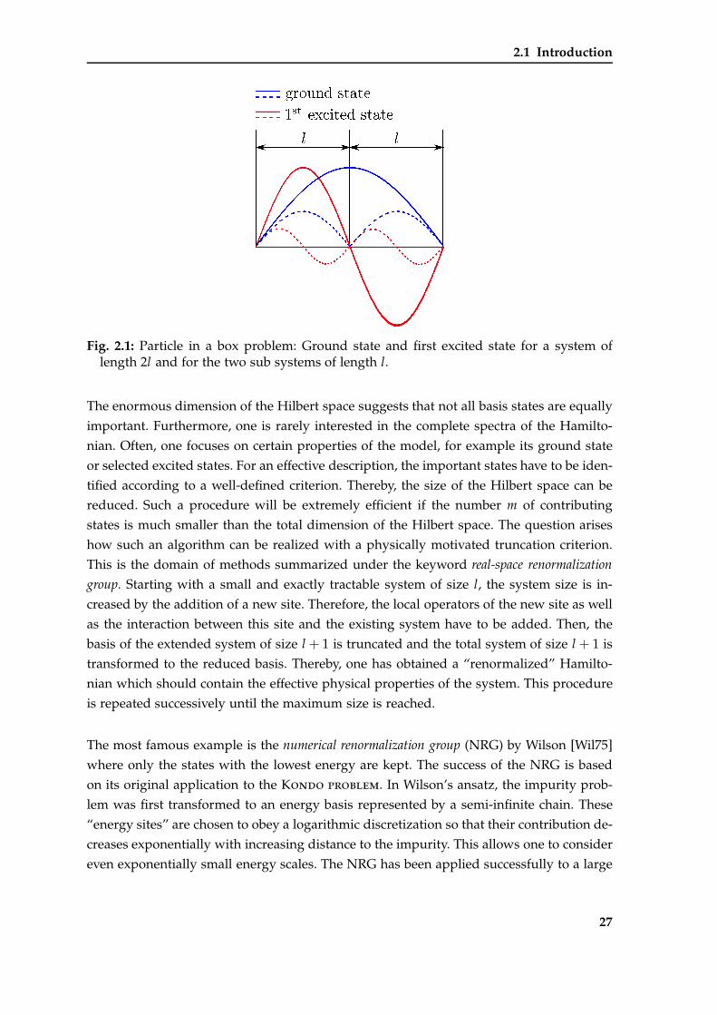
2.1 Introduction
Fig. 2.1: Particle in a box problem: Ground state and first excited state for a system oflength 2l and for the two sub systems of length l.
The enormous dimension of the Hilbert space suggests that not all basis states are equally
important. Furthermore, one is rarely interested in the complete spectra of the Hamilto-
nian. Often, one focuses on certain properties of the model, for example its ground state
or selected excited states. For an effective description, the important states have to be iden-
tified according to a well-defined criterion. Thereby, the size of the Hilbert space can be
reduced. Such a procedure will be extremely efficient if the number m of contributing
states is much smaller than the total dimension of the Hilbert space. The question arises
how such an algorithm can be realized with a physically motivated truncation criterion.
This is the domain of methods summarized under the keyword real-space renormalization
group. Starting with a small and exactly tractable system of size l, the system size is in-
creased by the addition of a new site. Therefore, the local operators of the new site as well
as the interaction between this site and the existing system have to be added. Then, the
basis of the extended system of size l + 1 is truncated and the total system of size l + 1 is
transformed to the reduced basis. Thereby, one has obtained a “renormalized” Hamilto-
nian which should contain the effective physical properties of the system. This procedure
is repeated successively until the maximum size is reached.
The most famous example is the numerical renormalization group (NRG) by Wilson [Wil75]
where only the states with the lowest energy are kept. The success of the NRG is based
on its original application to the Kondo problem. In Wilson’s ansatz, the impurity prob-
lem was first transformed to an energy basis represented by a semi-infinite chain. These
“energy sites” are chosen to obey a logarithmic discretization so that their contribution de-
creases exponentially with increasing distance to the impurity. This allows one to consider
even exponentially small energy scales. The NRG has been applied successfully to a large
27
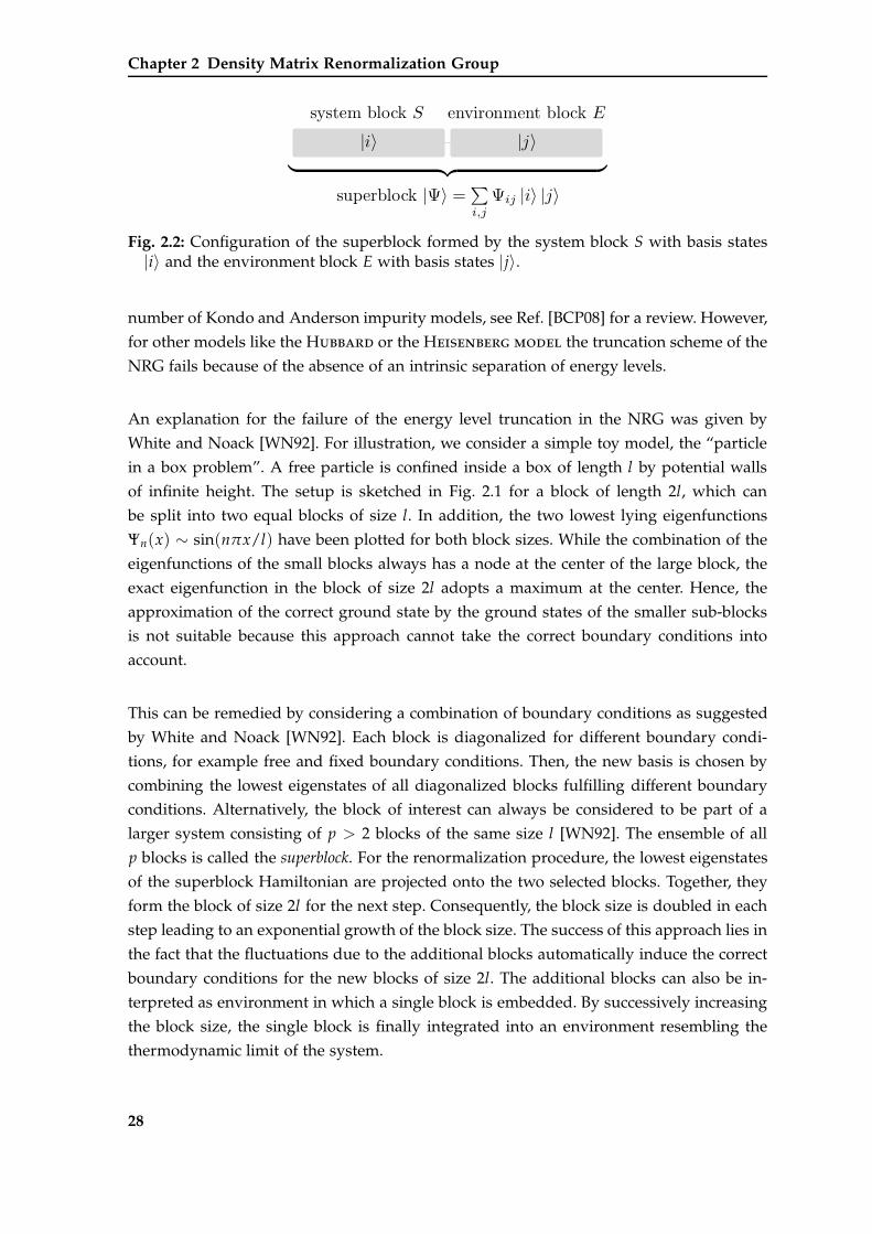
Chapter 2 Density Matrix Renormalization Group
Fig. 2.2: Configuration of the superblock formed by the system block S with basis states|i〉 and the environment block E with basis states |j〉.
number of Kondo and Anderson impurity models, see Ref. [BCP08] for a review. However,
for other models like the Hubbard or the Heisenberg model the truncation scheme of the
NRG fails because of the absence of an intrinsic separation of energy levels.
An explanation for the failure of the energy level truncation in the NRG was given by
White and Noack [WN92]. For illustration, we consider a simple toy model, the “particle
in a box problem”. A free particle is confined inside a box of length l by potential walls
of infinite height. The setup is sketched in Fig. 2.1 for a block of length 2l, which can
be split into two equal blocks of size l. In addition, the two lowest lying eigenfunctions
Ψn(x) ∼ sin(nπx/l) have been plotted for both block sizes. While the combination of the
eigenfunctions of the small blocks always has a node at the center of the large block, the
exact eigenfunction in the block of size 2l adopts a maximum at the center. Hence, the
approximation of the correct ground state by the ground states of the smaller sub-blocks
is not suitable because this approach cannot take the correct boundary conditions into
account.
This can be remedied by considering a combination of boundary conditions as suggested
by White and Noack [WN92]. Each block is diagonalized for different boundary condi-
tions, for example free and fixed boundary conditions. Then, the new basis is chosen by
combining the lowest eigenstates of all diagonalized blocks fulfilling different boundary
conditions. Alternatively, the block of interest can always be considered to be part of a
larger system consisting of p > 2 blocks of the same size l [WN92]. The ensemble of all
p blocks is called the superblock. For the renormalization procedure, the lowest eigenstates
of the superblock Hamiltonian are projected onto the two selected blocks. Together, they
form the block of size 2l for the next step. Consequently, the block size is doubled in each
step leading to an exponential growth of the block size. The success of this approach lies in
the fact that the fluctuations due to the additional blocks automatically induce the correct
boundary conditions for the new blocks of size 2l. The additional blocks can also be in-
terpreted as environment in which a single block is embedded. By successively increasing
the block size, the single block is finally integrated into an environment resembling the
thermodynamic limit of the system.
28
2.1 Introduction
A variation of the superblock method with linearly growing block size is the foundation of
DMRG [Whi92, Whi93]. We consider the setup shown in Fig. 2.2. The superblock consists
of a system block S with states |i〉 and an environment block E with states |j〉. The
state vector of the superblock
|Ψ〉 =dS,dE
∑i,j
Ψij |i〉 |j〉 (2.1)
is expressed in the product basis of S and E with coefficients Ψij. The number of states in
each block is given by the dimension of the corresponding Hilbert space, dS := dim HS and
dE := dim HE, respectively. The goal is to optimize the representation of the system block
by truncating the basis |i〉 according to a well-defined criterion. Thereby, the dimension
dS of the Hilbert space HS of the system block S is reduced. For an ideal representation
of the system block, the number of kept states m should be much smaller than its original
dimension dS. But what is an efficient criterion for the truncation? The optimization with
respect to the lowest lying energy levels as in NRG does not work well for models extended
in real space. Hence, one has to obey a different strategy. Let us specify the requirements
which have to be made to the truncation scheme. Ideally, it should
1) minimize the deviation of the optimized wave function from the exact one [Whi92,
Whi93],
2) lead to an optimal approximation of the expectation values [Whi98],
3) and preserve a maximum of the entanglement between system and environment
block [Gai01, GMD02, ON02, Gai03, LRV04].
2.1.1 Reduced density matrix
Before we present the different derivations leading to the DMRG truncation scheme,
we recapitulate the definition and the properties of a density matrix. They are essential
for the truncation scheme and can be found in any standard textbook, for example in
Ref. [Sch05b]. For a pure state as given in Eq. (2.1), the reduced density matrix of the system
block reads
ρS = TrE |Ψ〉 〈Ψ| (2.2)
where TrE denotes the partial trace over the environment block. For simplicity, we omit
the index S where this does not lead to confusion. Accordingly, a single element of the
29
Chapter 2 Density Matrix Renormalization Group
reduced density matrix is given by
ρii′ =dE
∑j
Ψ∗ijΨi′ j. (2.3)
The density matrix (2.2) fulfills the following properties:
Tr ρ = 1 (2.4a)
ρ† = ρ (2.4b)
ρ ≥ 0 ⇔ 〈ν|ρ|ν〉 ≥ 0 ∀ |ν〉 ∈ HS. (2.4c)
Hence, the density matrix is a normalized and diagonalizable operator. Due to its semi-
positive definiteness, all eigenvalues wi are greater than or equal to zero. Consequently, ρ
can be expressed in its eigenbasis
ρ =dS
∑i
wi |wi〉 〈wi| (2.5)
where wi can be regarded as the probability that ρ is in the eigenstate |wi〉. The inter-
pretation of the eigenvalues wi as probabilities is possible only because of the normaliza-
tion (2.4a) and the positive semi-definiteness (2.4c) of ρ. If |Ψ〉 is a pure state, the density
matrix is also a projector
ρ2 = ρ, (2.6)
which implies that all wi are either zero or unity. Furthermore, the expectation value of
any observable O from the system block can be expressed with the help of the density
matrix
〈O〉 = TrS ρO
=dS
∑i,i′
Oi′iρii′ .(2.7)
2.1.2 Truncation of the reduced density matrix
Now, we are able to address our previously made specifications which have to be fulfilled
by the DMRG truncation scheme. Each of the following derivations focuses on a different
property of the model, but all of them lead to the same criterion for the system block
optimization: The states with largest weight in the reduced density matrix of the system
block have to be kept.
30
2.1 Introduction
2.1.2.1 Optimization of the wave function
The derivation of the DMRG truncation from an optimization of the wave function was
first discussed by White when he introduced DMRG [Whi92, Whi93]. It relies on a varia-
tional optimization of the wave function. In the following, we present a slightly extended
derivation which is based on White’s original arguments. To this end, we define the trun-
cated wave function
|Ψ〉 =m,dE
∑α,j
cα,j |uα〉 |j〉 , (2.8)
where the basis |i〉 of the system block has been reduced to an m-dimensional basis
|uα〉 with |uα〉 = ∑dS
i ui,α |i〉 and m < dS.
For the following steps, it is advisable to rewrite the truncated state (2.8) as
|Ψ〉 =m
∑α
cα |uα〉 |vα〉 . (2.9)
The components of the vectors |vα〉 are defined by vα,j := 〈j|vα〉 = Nαcα,j. They are
normalized by choosing the constants Nα so that ∑dEj |vα,j|2 = 1.
The truncated state should approximate the exact state (2.1) as well as possible: |Ψ〉 ≈ |Ψ〉.Analytically, this is expressed as the minimization of the quadratic distance between the
exact and the truncated state
S :=∣∣∣|Ψ〉 − |Ψ〉
∣∣∣2
. (2.10)
After inserting (2.1) and (2.9), the quadratic distance is written as
S =dS,dE
∑i,j
(Ψij −
m
∑α
ui,αcαvj,α
)2
. (2.11)
This expression has to be minimized by varying over all cα, ui,α and vj,α. The uαshould form an orthonormal basis 〈uα|uα′〉 = δα,α′ . By interpreting the coefficients Ψijas elements of a rectangular dS × dE matrix, the minimization of the quadratic distance
can be understood as a component-by-component minimization of the individual matrix
elements. To solve this problem, we employ a singular value decomposition (SVD) to the
matrix Ψ = (Ψij) [PTVF07]. Then, the matrix Ψ is given by
Ψ = UDV⊤. (2.12)
31
Chapter 2 Density Matrix Renormalization Group
For simplicity, real valued matrices are assumed. But the argumentation holds for complex
matrices as well. Furthermore, we restrict ourselves to the case dS ≥ dE. The matrix D
is a diagonal dE × dE matrix containing the singular values of Ψ, while U is a column-
orthogonal dS × dE matrix and V⊤ is the transpose of an orthogonal dE × dE matrix V.
According to Eq. (2.11) the matrix elements of the truncated state Ψ read
Ψij :=m
∑α
ui,αcαvj,α
=dE
∑α
ui,αcαvj,α.
(2.13)
In the last step, the upper index of the sum has been extended to dE with cα = 0 for α > m.
In matrix form, one obtains
Ψ =
u1,1 · · · u1,dE
u2,1 · · · u2,dE
u3,1 · · · u3,dE...
......
udS,1 · · · udS,dE
·
c1 0. . . 0
0 cm
0 0
·
v1,1 · · · v1,dE
v2,1 · · · v2,dE
v3,1 · · · v3,dE...
......
vdE,1 · · · vdE,dE
⊤
. (2.14)
With respect to the minimization of Eq. (2.11), the columns |uα〉 and |vα〉 in the latter
expression for Ψ have to be the corresponding columns of U and V obtained from the SVD
of Ψ. Then, the truncated superblock state acquires the form
Ψ = UDV⊤ (2.15)
where
D =
c1 0. . . 0
0 cm
0 0
. (2.16)
is a diagonal matrix. In general, we could also assume that the matrix D is non-diagonal.
But the expression (2.13) for Ψ already implies that the non-diagonal elements have to be
zero. Hence, we directly define D as a diagonal matrix.
It is easily verified that the distance (2.11) expressed by the matrices Ψ and Ψ acquires the
32
2.1 Introduction
form
S = Tr(
Ψ − Ψ
) (Ψ − Ψ
)⊤. (2.17a)
After inserting the expressions for Ψ (2.12) and Ψ (2.15), the latter expression simplifies
to
S = Tr(
D − D)2
(2.17b)
because of the orthogonality of U and V. Both, D and D, are dE × dE matrices. But D only
contains m non-zero entries. In order to minimize the quadratic distance in Eq. (2.17b),
the diagonal entries cα of D have to be the largest m singular values of Ψ stored in the
matrix D. Now, we know how the distance S is minimized. But the SVD of Ψ still remains
to be calculated.
To this end, we consider
Ψ · Ψ⊤ = UD V⊤ · V︸ ︷︷ ︸
=1
D⊤U⊤
= UD2U⊤(2.18)
where the orthogonality of V has been exploited. The expression (2.18) is nothing else
but the reduced density matrix ρ of the system block, see Eq. (2.3). From Eq. (2.18), one
can draw two important conclusions. First, the matrix U diagonalizes the reduced density
matrix ρ. Hence, it contains the eigenstates |wα〉 of ρ as columns. The corresponding eigen-
values wα = c2α are the elements of the diagonal matrix D2. Second, the singular values
cα of Ψ are the square roots of the (positive) eigenvalues of ρ. Thereby, we have shown
that the optimal choice for the truncated basis of the system block are the m eigenstates of
the reduced density matrix ρ with largest eigenvalues wα. Ideally, the eigenvalues and the
corresponding eigenstates of ρ should be sorted in descending order w1 ≥ w2 ≥ . . . ≥ wdS
so that one can easily pick the m most important eigenstates.
A measure for the accuracy of the truncation is the discarded weight
err = 1 −m
∑α=1
wα (2.19)
where the sum runs over all weights of the regarded eigenstates. The discarded weight
defined in Eq. (2.19) is a measure for the weight of the truncated eigenstates because the
reduced density matrix is normalized according to Eq. (2.4a). Thus, a fast decay of the
eigenvalues with m is crucial for yielding a good accuracy. The derivation made above is
33
Chapter 2 Density Matrix Renormalization Group
almost identical for the second case where m < dS ≤ dE. Then, the last (dE − dS) columns
of U as well as the last m diagonal elements of D in (2.12) are zero.
Until now, the derivation of the density matrix criteria was made for a pure state |Ψ〉, for
example the ground state. If the state of the superblock is in a mixed state consisting of
several states |Ψk〉 with corresponding weights Wk, the optimal truncation scheme
is still described best by the eigenstates with largest weight in the reduced density ma-
trix [Whi93]. For a mixed state, the reduced density matrix is simply given as superposi-
tion
ρ = ∑k
Wkρk (2.20)
of the individual density matrices of the basis states |Ψk〉. Note that due to normalization
Tr ρk = 1 and ∑k Wk = 1 has to hold. Thus, the density matrix truncation is not restricted
to a single state. Several states can be targeted during a truncation. In the present thesis,
the use of several target states is exploited for the calculation of autocorrelation functions,
see Sect. 2.4.1.
2.1.2.2 Optimization of the expectation values
The density matrix criterion can also be derived from the expectation value of an arbitrary
observable O, which is contained in the system block [Whi98]. According to Eq. (2.7), the
expectation value of O is given by
〈O〉 = TrS ρO
=dS
∑α=1
wα 〈wα|O|wα〉 .(2.21)
In the last step, the representation of the reduced density matrix of the system block in its
eigenbasis has been inserted. As introduced in the previous section, we assume that the
eigenbasis of ρ is ordered in descending order with respect to its eigenvalues. Then, one
can simply truncate the sum in (2.21) after m eigenstates. This corresponds to a projection
onto the basis of the m most important eigenstates of ρ
〈O〉 =m
∑α=1
wα 〈wα|O|wα〉 . (2.22)
34
2.1 Introduction
Consequently, the deviation of the approximated expectation value from the exact one
reads
∣∣∣〈O〉 − 〈O〉∣∣∣ ≤ CO
dS
∑α=m+1
wα
≤ CO
(1 −
m
∑α=1
wα
)= CO · err
(2.23)
where CO := maxφ| 〈φ|O|φ〉 / 〈φ|φ〉 | is the norm of the observable O. Again, the error
can be estimated by the discarded weight defined in Eq. (2.19).
2.1.2.3 Preservation of the entanglement
Entanglement is a unique feature in quantum mechanics. Entangled states cannot be ex-
pressed as a tensor product of two sub states. For example, a spin singlet state or mS = 0
triplet state cannot be written as a simple product state of two spin-1/2 objects. The entan-
glement of a pure state consisting of two bipartite blocks has been studied in a variety of
works [Gai01, GMD02, ON02, Gai03, LRV04] and reveals a close relation between DMRG
and quantum information theory.
We start with the representation of the exact state |Ψ〉 in the basis of the system and
environment block (2.1) and recall the singular value decomposition of the matrix Ψ (2.12).
Thereby, one obtains
|Ψ〉 =dS,dE
∑i,j
dE
∑α
ui,α√
wαvj,α |i〉 |j〉
=dE
∑α=1
√wα
dS
∑i
ui,α |i〉
dE
∑j
vj,α |j〉
,
(2.24)
where dS ≥ dE has been assumed. The latter expression is equivalent to the Schmidt
decomposition [Sch07, NC10]
|Ψ〉 =r
∑α=1
√wα |wS
α〉 |wEα 〉 (2.25)
35
Chapter 2 Density Matrix Renormalization Group
of |Ψ〉 where the orthonormal basis states of the system and environment block
|wSα〉 =
dS
∑i
ui,α |i〉 (2.26a)
|wEα 〉 =
dE
∑j
vj,α |j〉 (2.26b)
are obtained from the projection of the orthonormal matrices U and V. The rank r corre-
sponds to the number of non-zero coefficients√
wα. For arbitrary values of dS and dE, it is
given by
r ≤ min(dS, dE
). (2.27)
The Schmidt decomposition also characterizes the entanglement of a bipartite state. Only
if r > 1, the two sub states are entangled. The reduced density matrices of the system and
the environment block read
ρS =r
∑α=1
wα |wSα〉 〈wS
α | (2.28a)
ρE =r
∑α=1
wα |wEα 〉 〈wE
α | . (2.28b)
The previous expressions are simply obtained from the total density matrix ρ = |Ψ〉 〈Ψ| by
inserting the Schmidt decomposition (2.25) and tracing out the environment or the system,
respectively. The latter result is consistent with the result from the optimization of the wave
function, see Sect. 2.1.2.1. The weights √wα of the decomposition are given by the square
roots of the eigenvalues wα of the reduced density matrix. The basis is formed by the
eigenstates of the system and environment block, respectively. In addition, the Schmidt
decomposition implies that the eigenvalues of the system and the environment block are
identical even if both blocks are different. Their number is given by the rank r, which
corresponds to the dimension of the smaller block.
The entanglement is measured by the von Neumann entropy
SN = −Tr ρ ln ρ
= −r
∑α=1
wα ln wα.(2.29)
As before, we assume that the eigenvalues wα are ordered with decreasing magnitude
w1 ≥ w2 ≥ . . . ≥ wr. The expression −x ln x in the von Neumann entropy (2.29) is a mono-
tonically growing function for 0 < x ≤ 1/ e, where the upper limit 1/ e is much larger than
36
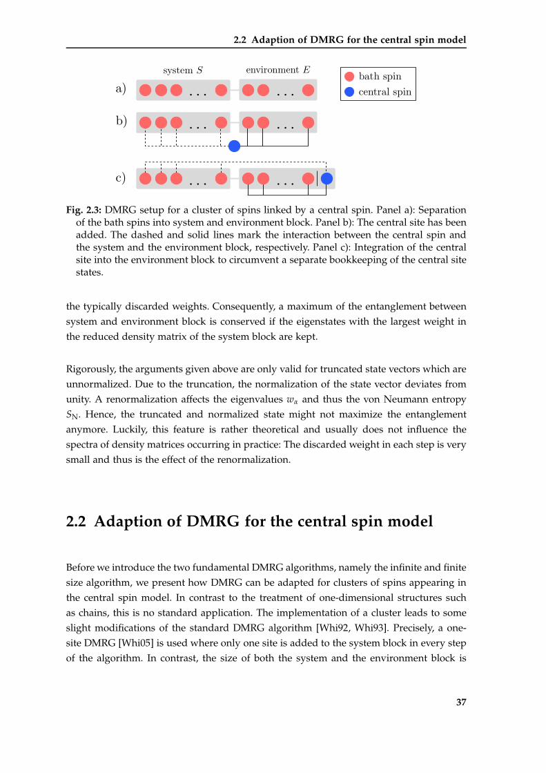
2.2 Adaption of DMRG for the central spin model
Fig. 2.3: DMRG setup for a cluster of spins linked by a central spin. Panel a): Separationof the bath spins into system and environment block. Panel b): The central site has beenadded. The dashed and solid lines mark the interaction between the central spin andthe system and the environment block, respectively. Panel c): Integration of the centralsite into the environment block to circumvent a separate bookkeeping of the central sitestates.
the typically discarded weights. Consequently, a maximum of the entanglement between
system and environment block is conserved if the eigenstates with the largest weight in
the reduced density matrix of the system block are kept.
Rigorously, the arguments given above are only valid for truncated state vectors which are
unnormalized. Due to the truncation, the normalization of the state vector deviates from
unity. A renormalization affects the eigenvalues wα and thus the von Neumann entropy
SN. Hence, the truncated and normalized state might not maximize the entanglement
anymore. Luckily, this feature is rather theoretical and usually does not influence the
spectra of density matrices occurring in practice: The discarded weight in each step is very
small and thus is the effect of the renormalization.
2.2 Adaption of DMRG for the central spin model
Before we introduce the two fundamental DMRG algorithms, namely the infinite and finite
size algorithm, we present how DMRG can be adapted for clusters of spins appearing in
the central spin model. In contrast to the treatment of one-dimensional structures such
as chains, this is no standard application. The implementation of a cluster leads to some
slight modifications of the standard DMRG algorithm [Whi92, Whi93]. Precisely, a one-
site DMRG [Whi05] is used where only one site is added to the system block in every step
of the algorithm. In contrast, the size of both the system and the environment block is
37
Chapter 2 Density Matrix Renormalization Group
extended by one site in every step of the standard two-site DMRG.
First, we neglect the central spin and only consider the bath spins. They can be viewed as
a non-interacting chain of spins, which can be split into the DMRG setup of system and
environment block, as described in Sect. 2.1 and sketched in panel a) of Fig. 2.3.
Now, we have to add the central spin to the non-interacting bath spins. The key point for
the success of the algorithm lies in the exact treatment of the central spin so that the DMRG
only needs to optimize the representation of the bath spins. By keeping the central spin
separate from the bath spins, its operators and thus the interaction with the surrounding
bath spins is treated exactly. The separated central spin and its interaction with the bath
spins is illustrated in panel b) of Fig. 2.3. Hence, the state vector of the superblock (2.1)
can now be written as
|Ψ〉 = ∑i,j,σ0
Ψσ0ij |i〉 |j〉 |σ0〉 , (2.30)
which corresponds to a representation with three basis sets: System block, environment
block, and the central spin. In this notation, the Hamiltonian HS of the system block as
well as the Hamiltonian HE are both always zero or contain only local contributions, for
example from external fields applied to the bath spins. The interaction between central
spin and bath is only established when the action of the superblock Hamiltonian onto the
superblock state vector is required.
The employment of three basis sets is rather unhandy. To circumvent the bookkeeping for
the central site state, it is convenient to integrate the central site into the environment as
shown in panel c) of Fig. 2.3. Then, the state of the superblock is given as
|Ψ〉 = ∑i,j
Ψij |i〉 |j〉 (2.31)
where |j〉 = |j〉 ⊗ |σ0〉 is the basis of the environment including the central site and (Ψij)
a dS × 2dE matrix containing the coefficients. The new quantum numbers j are obtained
from the extension of the environment basis with the two basis states |↑〉 and |↓〉 of the
central site. In this approach, the interactions in HE are established when the central site
is added to the environment block. The system block Hamiltonian is still always zero,
despite possible local contributions.
For the buildup of the superblock, one starts with a system and environment block of the
same size which contain an exactly tractable number of spins. The number of bath spins in
the environment block is fixed, while two sites have to be added to the blocks in each step
38
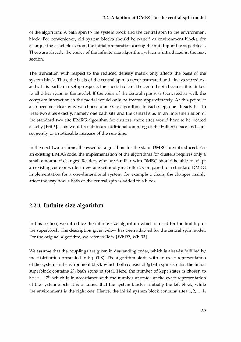
2.2 Adaption of DMRG for the central spin model
of the algorithm: A bath spin to the system block and the central spin to the environment
block. For convenience, old system blocks should be reused as environment blocks, for
example the exact block from the initial preparation during the buildup of the superblock.
These are already the basics of the infinite size algorithm, which is introduced in the next
section.
The truncation with respect to the reduced density matrix only affects the basis of the
system block. Thus, the basis of the central spin is never truncated and always stored ex-
actly. This particular setup respects the special role of the central spin because it is linked
to all other spins in the model. If the basis of the central spin was truncated as well, the
complete interaction in the model would only be treated approximately. At this point, it
also becomes clear why we choose a one-site algorithm. In each step, one already has to
treat two sites exactly, namely one bath site and the central site. In an implementation of
the standard two-site DMRG algorithm for clusters, three sites would have to be treated
exactly [Fri06]. This would result in an additional doubling of the Hilbert space and con-
sequently to a noticeable increase of the run-time.
In the next two sections, the essential algorithms for the static DMRG are introduced. For
an existing DMRG code, the implementation of the algorithms for clusters requires only a
small amount of changes. Readers who are familiar with DMRG should be able to adapt
an existing code or write a new one without great effort. Compared to a standard DMRG
implementation for a one-dimensional system, for example a chain, the changes mainly
affect the way how a bath or the central spin is added to a block.
2.2.1 Infinite size algorithm
In this section, we introduce the infinite size algorithm which is used for the buildup of
the superblock. The description given below has been adapted for the central spin model.
For the original algorithm, we refer to Refs. [Whi92, Whi93].
We assume that the couplings are given in descending order, which is already fulfilled by
the distribution presented in Eq. (1.8). The algorithm starts with an exact representation
of the system and environment block which both consist of l0 bath spins so that the initial
superblock contains 2l0 bath spins in total. Here, the number of kept states is chosen to
be m ≡ 2l0 which is in accordance with the number of states of the exact representation
of the system block. It is assumed that the system block is initially the left block, while
the environment is the right one. Hence, the initial system block contains sites 1, 2, . . . l0
39
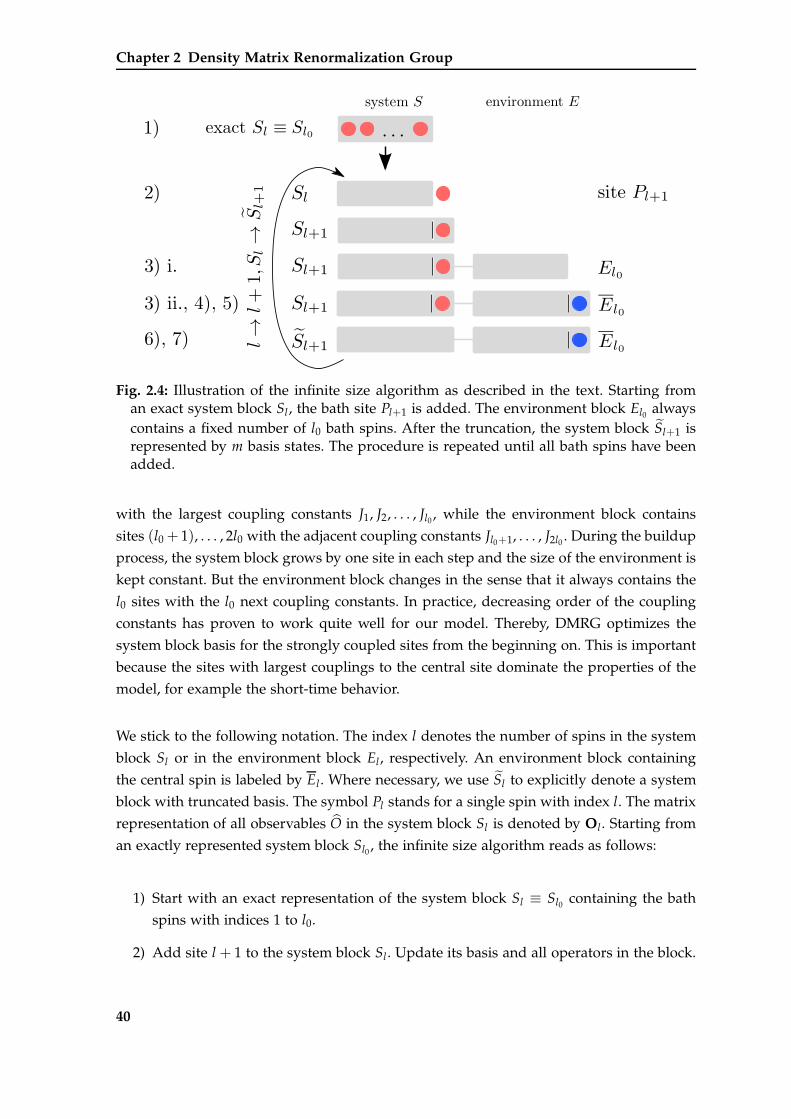
Chapter 2 Density Matrix Renormalization Group
Fig. 2.4: Illustration of the infinite size algorithm as described in the text. Starting froman exact system block Sl, the bath site Pl+1 is added. The environment block El0 alwayscontains a fixed number of l0 bath spins. After the truncation, the system block Sl+1 isrepresented by m basis states. The procedure is repeated until all bath spins have beenadded.
with the largest coupling constants J1, J2, . . . , Jl0 , while the environment block contains
sites (l0 + 1), . . . , 2l0 with the adjacent coupling constants Jl0+1, . . . , J2l0 . During the buildup
process, the system block grows by one site in each step and the size of the environment is
kept constant. But the environment block changes in the sense that it always contains the
l0 sites with the l0 next coupling constants. In practice, decreasing order of the coupling
constants has proven to work quite well for our model. Thereby, DMRG optimizes the
system block basis for the strongly coupled sites from the beginning on. This is important
because the sites with largest couplings to the central site dominate the properties of the
model, for example the short-time behavior.
We stick to the following notation. The index l denotes the number of spins in the system
block Sl or in the environment block El, respectively. An environment block containing
the central spin is labeled by El. Where necessary, we use Sl to explicitly denote a system
block with truncated basis. The symbol Pl stands for a single spin with index l. The matrix
representation of all observables O in the system block Sl is denoted by Ol. Starting from
an exactly represented system block Sl0 , the infinite size algorithm reads as follows:
1) Start with an exact representation of the system block Sl ≡ Sl0 containing the bath
spins with indices 1 to l0.
2) Add site l + 1 to the system block Sl. Update its basis and all operators in the block.
40
2.2 Adaption of DMRG for the central spin model
3) Representation of the environment block El0 :
i. Create an exact environment block El0 containing the bath spins with indices
(l + 2) to (l + l0 + 1).
ii. Add central spin to the environment block. Update its basis and all correspond-
ing operators.
4) Calculate all desired target states, for example the ground state.
5) Perform measurements, for example the ground state energy or the magnetization.
6) Basis optimization of the system block:
i. Use target states to set up the reduced density matrix ρ (2.3) of the system block
and diagonalize it.
ii. Choose the m eigenstates with largest weight in the reduced density matrix.
Truncate the basis of the system block and all corresponding operators via
Ψl+1 = UΨl+1U† (2.32a)
Ol+1 = UOl+1U† (2.32b)
where the transformation U contains the largest m eigenvectors as columns.
7) Continue at step 2) replacing l → l + 1 and Sl → Sl+1 until all N bath spins have
been added to the superblock.
There are two strategies for the calculation of the target states. First, the target state can
be constructed from a tensor product of the local states of all spins. For example, the
(random) initial state of every bath site can be parameterized on the Bloch sphere. When
the site Pl+1 is added to the system block, its state has to be added to the state vector by
calculating the tensor product between the state of the system block Sl and the state of the
single site Pl+1.
Second, one can calculate the target state as the ground state of a specific Hamiltonian.
This corresponds to the standard application of DMRG for determining the ground state
properties of a model. But note that the Hamiltonian for the initialization does not have
to be the actual Hamiltonian of the model. For example, one can apply the simple Hamil-
tonian H = −N
∑i=0
hiSzi with |hi| ≫ 1 [GKSS05]. In the corresponding ground state, each
spin is in a completely polarized state according to the sign of hi. If possible, we usually
employ the first approach based on the tensor product of the local states to avoid the costly
calculation of the ground state.
41
Chapter 2 Density Matrix Renormalization Group
The ground state may be calculated by the well-known Lanczos algorithm [Lan50]. This
iterative algorithm requires a repetitive calculation, typically O(100), of the action of the
superblock Hamiltonian HSB
HSB = HS ⊗ 1E + 1S ⊗ HE + ∑i∈S
Ji~Si,S ⊗ ~S0,E (2.33)
on the state |Ψ〉, which is the numerically most costly operation. Here, HS is the Hamil-
tonian of the system block consisting of only local contributions, while the Hamiltonian
HE contains already the interaction between central spin and bath spins from the environ-
ment block. The sum in Eq. (2.33) involves all links between central spin and bath spins
from the system block. In general, the Hamiltonian HSB should never be stored due to its
enormous size. Instead, one directly evaluates the action of the superblock Hamiltonian
by the relation [PKWH99, Chapter 2]
(HSBΨ)ij = ∑i′,j′
(HSB)ij;i′ j′ Ψi′ ,j′
= ∑λ
∑i′
OS,λii′ ∑
j′OE,λ
jj′ Ψi′ ,j′ .(2.34)
In the last step, the representation
(HSB)ij;i′ j′ = ∑λ
OS,λii′ OE,λ
jj′ (2.35)
of the superblock Hamiltonian is inserted. The sum runs over all pairs of operators OS,λ
and OE,λ forming the superblock Hamiltonian HSB (2.33). The operator OS,λ denotes the
operator from the system block, while OE,λ stands for the corresponding operator from
the environment block. The direct evaluation of the action decreases the numerical effort
by one order of magnitude to O(m3). A naive application of HSB onto the state vector
would imply an effort of O(m4) because the dimension of the superblock Hamiltonian is
quadratic in the number of states m. In practice, the numerical effort can even be reduced
below O(m3) if the symmetries of the model under study are exploited.
In the central spin model as defined in Eqs. (1.4) and (1.6), the total magnetization ∑Ni=0 Sz
i
is always conserved. Hence, it is a good quantum number and can be used to index the
basis of the blocks. Then, the state vector and all operators take the form of block matrices.
Most blocks are empty so they do not have to be stored, while the non-empty blocks are
represented by dense matrices. All matrix-matrix and matrix-vector multiplications require
an additional loop over the good quantum number. As the good quantum is conserved
and many blocks are zero, the multiplication of very large matrices is reduced to multiple
multiplications of matrices with a much smaller dimension. This induces a noticeable
increase of the performance.
42
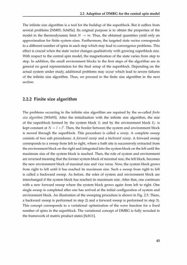
2.2 Adaption of DMRG for the central spin model
The infinite size algorithm is a tool for the buildup of the superblock. But it suffers from
several problems [NM05, Sch05a]. Its original purpose is to obtain the properties of the
model in the thermodynamic limit N → ∞. Thus, the obtained quantities yield only an
approximation for finite system sizes. Furthermore, the targeted state vector corresponds
to a different number of spins in each step which may lead to convergence problems. This
effect is crucial when the state vector changes qualitatively with growing superblock size.
With respect to the central spin model, the magnetization of the state varies from step to
step. In addition, the small environment blocks in the first steps of the algorithm are in
general no good representation for the final setup of the superblock. Depending on the
actual system under study, additional problems may occur which lead to severe failures
of the infinite size algorithm. Thus, we proceed to the finite size algorithm in the next
section.
2.2.2 Finite size algorithm
The problems occurring in the infinite size algorithm are repaired by the so-called finite
size algorithm [Whi93]. After the initialization with the infinite size algorithm, the size
of the superblock formed by the system block Sl and by the environment block El′ is
kept constant at N = l + l′. Then, the border between the system and environment block
is moved through the superblock. This procedure is called a sweep. A complete sweep
consists of two sub procedures: A forward sweep and a backward sweep. A forward sweep
corresponds to a sweep from left to right, where a bath site is successively extracted from
the environment block on the right and integrated into the system block on the left until the
maximum size of the system block is reached. Then, the role of system and environment
are reversed meaning that the former system block of maximal size, the left block, becomes
the new environment block of maximal size and vice versa. Now, the system block grows
from right to left until it has reached its maximum size. Such a sweep from right to left
is called a backward sweep. As before, the roles of system and environment block are
interchanged if the system block has reached its maximum size. After that, one continues
with a new forward sweep where the system block grows again from left to right. One
single sweep is completed after one has arrived at the initial configuration of system and
environment block. An illustration of the sweeping procedure is shown in Fig. 2.5. There,
a backward sweep is performed in step 2) and a forward sweep is performed in step 3).
This concept corresponds to a variational optimization of the wave function for a fixed
number of spins in the superblock. The variational concept of DMRG is fully revealed in
the framework of matrix product states [Sch11].
43
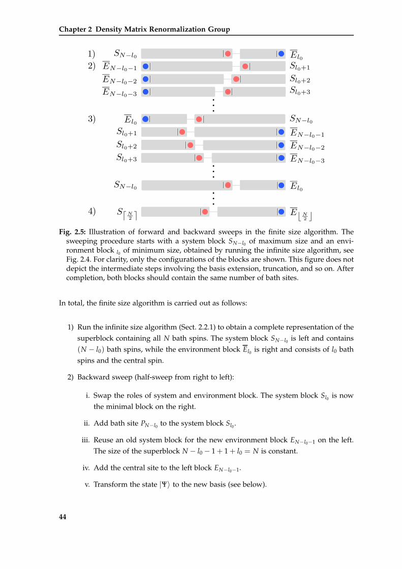
Chapter 2 Density Matrix Renormalization Group
Fig. 2.5: Illustration of forward and backward sweeps in the finite size algorithm. Thesweeping procedure starts with a system block SN−l0 of maximum size and an envi-ronment block l0 of minimum size, obtained by running the infinite size algorithm, seeFig. 2.4. For clarity, only the configurations of the blocks are shown. This figure does notdepict the intermediate steps involving the basis extension, truncation, and so on. Aftercompletion, both blocks should contain the same number of bath sites.
In total, the finite size algorithm is carried out as follows:
1) Run the infinite size algorithm (Sect. 2.2.1) to obtain a complete representation of the
superblock containing all N bath spins. The system block SN−l0 is left and contains
(N − l0) bath spins, while the environment block El0 is right and consists of l0 bath
spins and the central spin.
2) Backward sweep (half-sweep from right to left):
i. Swap the roles of system and environment block. The system block Sl0 is now
the minimal block on the right.
ii. Add bath site PN−l0 to the system block Sl0 .
iii. Reuse an old system block for the new environment block EN−l0−1 on the left.
The size of the superblock N − l0 − 1 + 1 + l0 = N is constant.
iv. Add the central site to the left block EN−l0−1.
v. Transform the state |Ψ〉 to the new basis (see below).
44
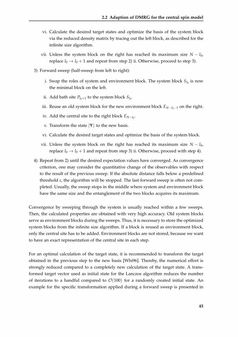
2.2 Adaption of DMRG for the central spin model
vi. Calculate the desired target states and optimize the basis of the system block
via the reduced density matrix by tracing out the left block, as described for the
infinite size algorithm.
vii. Unless the system block on the right has reached its maximum size N − l0,
replace l0 → l0 + 1 and repeat from step 2) ii. Otherwise, proceed to step 3).
3) Forward sweep (half-sweep from left to right):
i. Swap the roles of system and environment block. The system block Sl0 is now
the minimal block on the left.
ii. Add bath site Pl0+1 to the system block Sl0 .
iii. Reuse an old system block for the new environment block EN−l0−1 on the right.
iv. Add the central site to the right block EN−l0 .
v. Transform the state |Ψ〉 to the new basis.
vi. Calculate the desired target states and optimize the basis of the system block.
vii. Unless the system block on the right has reached its maximum size N − l0,
replace l0 → l0 + 1 and repeat from step 3) ii. Otherwise, proceed with step 4).
4) Repeat from 2) until the desired expectation values have converged. As convergence
criterion, one may consider the quantitative change of the observables with respect
to the result of the previous sweep. If the absolute distance falls below a predefined
threshold ε, the algorithm will be stopped. The last forward sweep is often not com-
pleted. Usually, the sweep stops in the middle where system and environment block
have the same size and the entanglement of the two blocks acquires its maximum.
Convergence by sweeping through the system is usually reached within a few sweeps.
Then, the calculated properties are obtained with very high accuracy. Old system blocks
serve as environment blocks during the sweeps. Thus, it is necessary to store the optimized
system blocks from the infinite size algorithm. If a block is reused as environment block,
only the central site has to be added. Environment blocks are not stored, because we want
to have an exact representation of the central site in each step.
For an optimal calculation of the target state, it is recommended to transform the target
obtained in the previous step to the new basis [Whi96]. Thereby, the numerical effort is
strongly reduced compared to a completely new calculation of the target state. A trans-
formed target vector used as initial state for the Lanczos algorithm reduces the number
of iterations to a handful compared to O(100) for a randomly created initial state. An
example for the specific transformation applied during a forward sweep is presented in
45
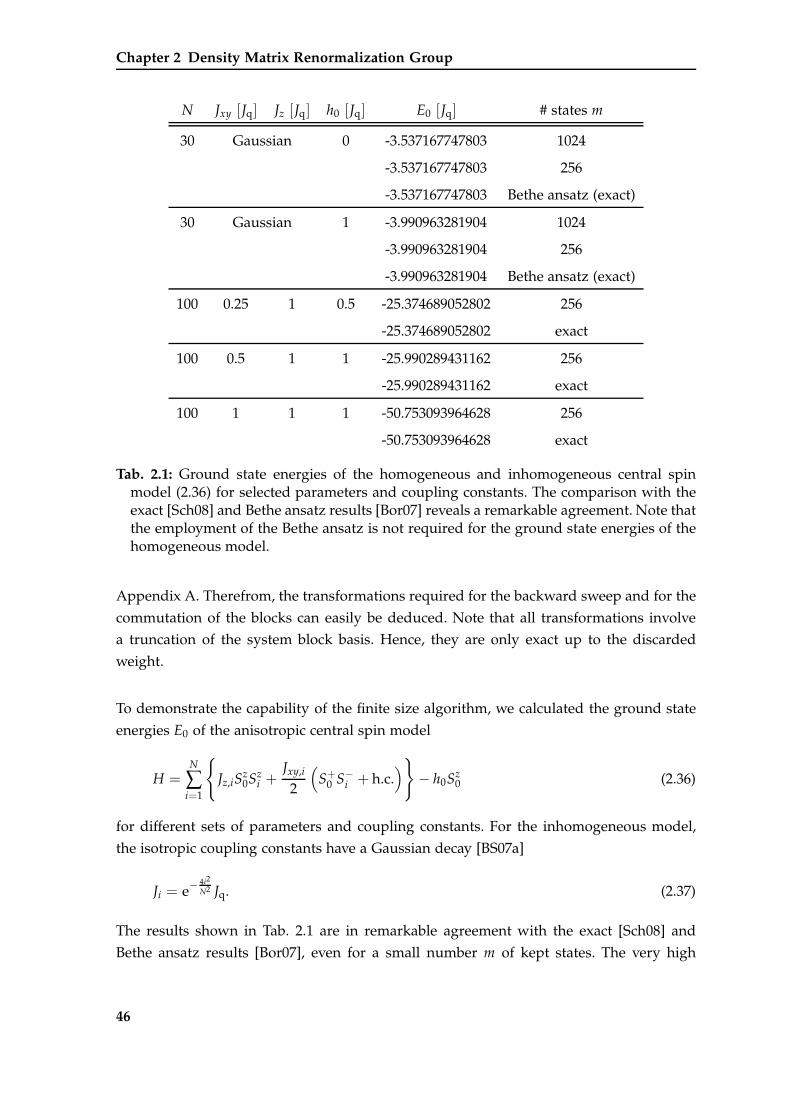
Chapter 2 Density Matrix Renormalization Group
N Jxy [Jq] Jz [Jq] h0 [Jq] E0 [Jq] # states m
30 Gaussian 0 -3.537167747803 1024
-3.537167747803 256
-3.537167747803 Bethe ansatz (exact)
30 Gaussian 1 -3.990963281904 1024
-3.990963281904 256
-3.990963281904 Bethe ansatz (exact)
100 0.25 1 0.5 -25.374689052802 256
-25.374689052802 exact
100 0.5 1 1 -25.990289431162 256
-25.990289431162 exact
100 1 1 1 -50.753093964628 256
-50.753093964628 exact
Tab. 2.1: Ground state energies of the homogeneous and inhomogeneous central spinmodel (2.36) for selected parameters and coupling constants. The comparison with theexact [Sch08] and Bethe ansatz results [Bor07] reveals a remarkable agreement. Note thatthe employment of the Bethe ansatz is not required for the ground state energies of thehomogeneous model.
Appendix A. Therefrom, the transformations required for the backward sweep and for the
commutation of the blocks can easily be deduced. Note that all transformations involve
a truncation of the system block basis. Hence, they are only exact up to the discarded
weight.
To demonstrate the capability of the finite size algorithm, we calculated the ground state
energies E0 of the anisotropic central spin model
H =N
∑i=1
Jz,iS
z0Sz
i +Jxy,i
2
(S+
0 S−i + h.c.
)− h0Sz
0 (2.36)
for different sets of parameters and coupling constants. For the inhomogeneous model,
the isotropic coupling constants have a Gaussian decay [BS07a]
Ji = e−4i2
N2 Jq. (2.37)
The results shown in Tab. 2.1 are in remarkable agreement with the exact [Sch08] and
Bethe ansatz results [Bor07], even for a small number m of kept states. The very high
46
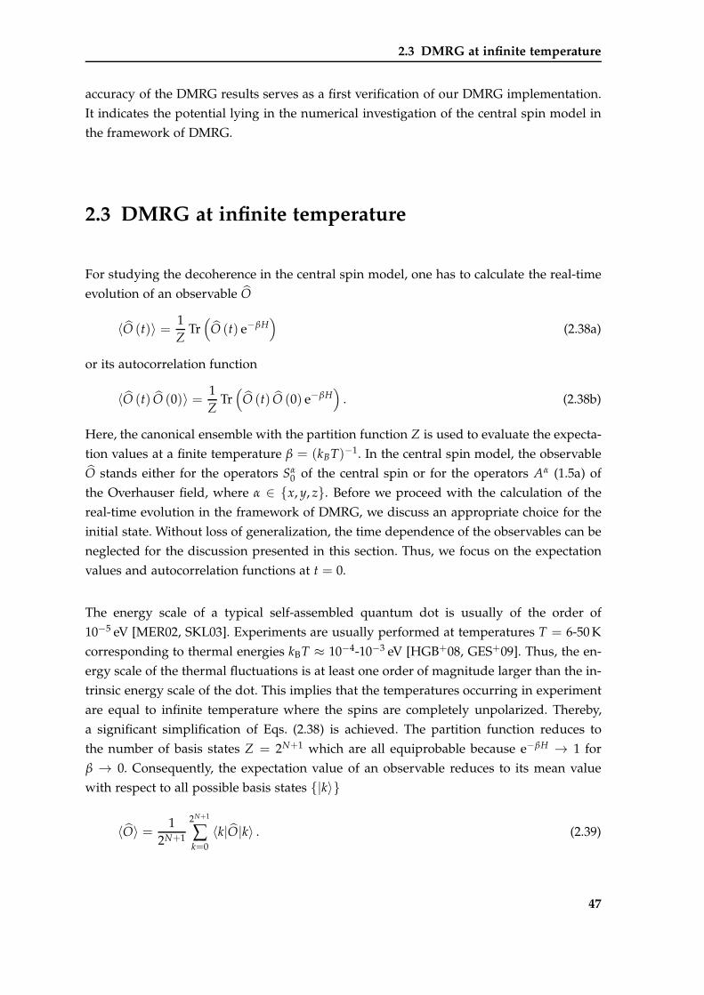
2.3 DMRG at infinite temperature
accuracy of the DMRG results serves as a first verification of our DMRG implementation.
It indicates the potential lying in the numerical investigation of the central spin model in
the framework of DMRG.
2.3 DMRG at infinite temperature
For studying the decoherence in the central spin model, one has to calculate the real-time
evolution of an observable O
〈O (t)〉 = 1Z
Tr(
O (t) e−βH)
(2.38a)
or its autocorrelation function
〈O (t) O (0)〉 = 1Z
Tr(
O (t) O (0) e−βH)
. (2.38b)
Here, the canonical ensemble with the partition function Z is used to evaluate the expecta-
tion values at a finite temperature β = (kBT)−1. In the central spin model, the observable
O stands either for the operators Sα0 of the central spin or for the operators Aα (1.5a) of
the Overhauser field, where α ∈ x, y, z. Before we proceed with the calculation of the
real-time evolution in the framework of DMRG, we discuss an appropriate choice for the
initial state. Without loss of generalization, the time dependence of the observables can be
neglected for the discussion presented in this section. Thus, we focus on the expectation
values and autocorrelation functions at t = 0.
The energy scale of a typical self-assembled quantum dot is usually of the order of
10−5 eV [MER02, SKL03]. Experiments are usually performed at temperatures T = 6-50 K
corresponding to thermal energies kBT ≈ 10−4-10−3 eV [HGB+08, GES+09]. Thus, the en-
ergy scale of the thermal fluctuations is at least one order of magnitude larger than the in-
trinsic energy scale of the dot. This implies that the temperatures occurring in experiment
are equal to infinite temperature where the spins are completely unpolarized. Thereby,
a significant simplification of Eqs. (2.38) is achieved. The partition function reduces to
the number of basis states Z = 2N+1 which are all equiprobable because e−βH → 1 for
β → 0. Consequently, the expectation value of an observable reduces to its mean value
with respect to all possible basis states |k〉
〈O〉 = 12N+1
2N+1
∑k=0
〈k|O|k〉 . (2.39)
47
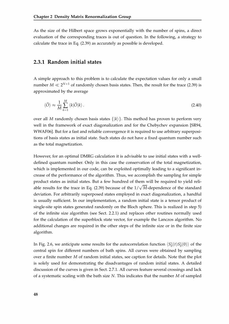
Chapter 2 Density Matrix Renormalization Group
As the size of the Hilbert space grows exponentially with the number of spins, a direct
evaluation of the corresponding traces is out of question. In the following, a strategy to
calculate the trace in Eq. (2.39) as accurately as possible is developed.
2.3.1 Random initial states
A simple approach to this problem is to calculate the expectation values for only a small
number M ≪ 2N+1 of randomly chosen basis states. Then, the result for the trace (2.39) is
approximated by the average
〈O〉 ≈ 1M
M
∑k=1
〈k|O|k〉 . (2.40)
over all M randomly chosen basis states |k〉. This method has proven to perform very
well in the framework of exact diagonalization and for the Chebychev expansion [SR94,
WWAF06]. But for a fast and reliable convergence it is required to use arbitrary superposi-
tions of basis states as initial state. Such states do not have a fixed quantum number such
as the total magnetization.
However, for an optimal DMRG calculation it is advisable to use initial states with a well-
defined quantum number. Only in this case the conservation of the total magnetization,
which is implemented in our code, can be exploited optimally leading to a significant in-
crease of the performance of the algorithm. Thus, we accomplish the sampling for simple
product states as initial states. But a few hundred of them will be required to yield reli-
able results for the trace in Eq. (2.39) because of the 1/√
M-dependence of the standard
deviation. For arbitrarily superposed states employed in exact diagonalization, a handful
is usually sufficient. In our implementation, a random initial state is a tensor product of
single-site spin states generated randomly on the Bloch sphere. This is realized in step 5)
of the infinite size algorithm (see Sect. 2.2.1) and replaces other routines normally used
for the calculation of the superblock state vector, for example the Lanczos algorithm. No
additional changes are required in the other steps of the infinite size or in the finite size
algorithm.
In Fig. 2.6, we anticipate some results for the autocorrelation function 〈Sz0(t)S
z0(0)〉 of the
central spin for different numbers of bath spins. All curves were obtained by sampling
over a finite number M of random initial states, see caption for details. Note that the plot
is solely used for demonstrating the disadvantages of random initial states. A detailed
discussion of the curves is given in Sect. 2.7.1. All curves feature several crossings and lack
of a systematic scaling with the bath size N. This indicates that the number M of sampled
48
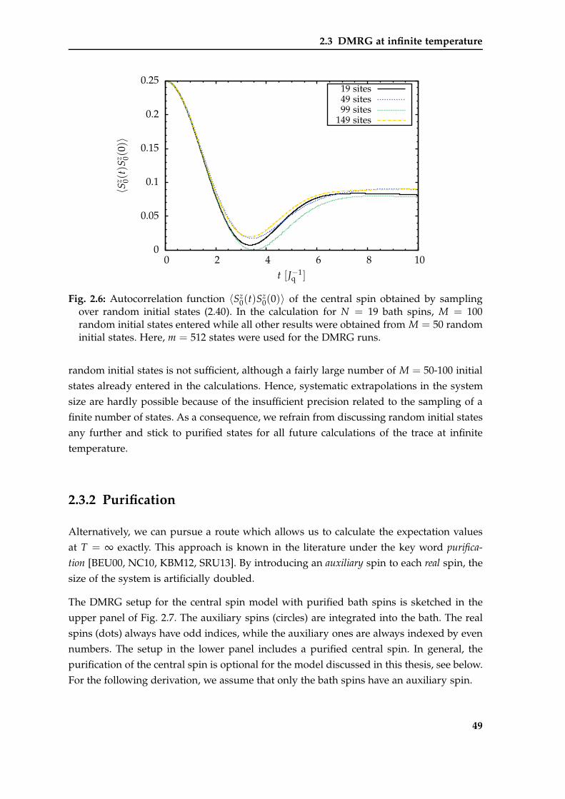
2.3 DMRG at infinite temperature
0
0.05
0.1
0.15
0.2
0.25
0 2 4 6 8 10
〈Sz 0(
t)S
z 0(0)〉
t [J−1q ]
19 sites49 sites99 sites
149 sites
Fig. 2.6: Autocorrelation function 〈Sz0(t)S
z0(0)〉 of the central spin obtained by sampling
over random initial states (2.40). In the calculation for N = 19 bath spins, M = 100random initial states entered while all other results were obtained from M = 50 randominitial states. Here, m = 512 states were used for the DMRG runs.
random initial states is not sufficient, although a fairly large number of M = 50-100 initial
states already entered in the calculations. Hence, systematic extrapolations in the system
size are hardly possible because of the insufficient precision related to the sampling of a
finite number of states. As a consequence, we refrain from discussing random initial states
any further and stick to purified states for all future calculations of the trace at infinite
temperature.
2.3.2 Purification
Alternatively, we can pursue a route which allows us to calculate the expectation values
at T = ∞ exactly. This approach is known in the literature under the key word purifica-
tion [BEU00, NC10, KBM12, SRU13]. By introducing an auxiliary spin to each real spin, the
size of the system is artificially doubled.
The DMRG setup for the central spin model with purified bath spins is sketched in the
upper panel of Fig. 2.7. The auxiliary spins (circles) are integrated into the bath. The real
spins (dots) always have odd indices, while the auxiliary ones are always indexed by even
numbers. The setup in the lower panel includes a purified central spin. In general, the
purification of the central spin is optional for the model discussed in this thesis, see below.
For the following derivation, we assume that only the bath spins have an auxiliary spin.
49
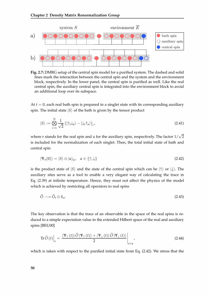
Chapter 2 Density Matrix Renormalization Group
Fig. 2.7: DMRG setup of the central spin model for a purified system. The dashed and solidlines mark the interaction between the central spin and the system and the environmentblock, respectively. In the lower panel, the central spin is purified as well. Like the realcentral spin, the auxiliary central spin is integrated into the environment block to avoidan additional loop over its subspace.
At t = 0, each real bath spin is prepared in a singlet state with its corresponding auxiliary
spin. The initial state |S〉 of the bath is given by the tensor product
|S〉 :=N⊗
i=1
1√2
(|↑r↓a〉 − |↓r↑a〉
)i, (2.41)
where r stands for the real spin and a for the auxiliary spin, respectively. The factor 1/√
2
is included for the normalization of each singlet. Then, the total initial state of bath and
central spin
|Ψα(0)〉 = |S〉 ⊗ |α〉0 , α ∈ ↑, ↓ (2.42)
is the product state of |S〉 and the state of the central spin which can be |↑〉 or |↓〉. The
auxiliary sites serve as a tool to enable a very elegant way of calculating the trace in
Eq. (2.39) at infinite temperature. Hence, they must not affect the physics of the model
which is achieved by restricting all operators to real spins
O −→ Or ⊗ 1a. (2.43)
The key observation is that the trace of an observable in the space of the real spins is re-
duced to a simple expectation value in the extended Hilbert space of the real and auxiliary
spins [BEU00]
Tr O (t)∣∣∣r=
〈Ψ↑ (t)| O |Ψ↑ (t)〉+ 〈Ψ↓ (t)| O |Ψ↓ (t)〉2
∣∣∣∣∣r⊗a
, (2.44)
which is taken with respect to the purified initial state from Eq. (2.42). We stress that the
50
2.3 DMRG at infinite temperature
latter expression allows for an exact calculation of the trace with only two independent
runs of the DMRG code, one for each state of the central spin. If the central spin would be
purified as well, the result would be yield within a single run.
Without any external field, the central spin model in Eq. (1.4) is isotropic and symmetric
under a spin flip of the central spin. Thus, a purification of the central spin is not neces-
sary and it is sufficient to consider only one initial state where the central spin at t = 0
points either up or down because of the spin-flip symmetry. If the spin-flip symmetry is
broken by an external magnetic field, one has to run two independent calculations for both
states of the central spin. The total trace is simply given as the mean value of two inde-
pendent results. Compared to a calculation with a purified central spin, the dimension of
the Hilbert space is kept smaller by a factor of two resulting in a decrease of the discarded
weight and an overall better performance, see Sect. 2.5.3. However, a purified central spin
gives access to conceptual extensions of DMRG. Hence, we come back to this concept for
the discussion of the Chebychev polynomials in Sect. 2.4.4.
Although a purified initial state (2.42) implies an additional doubling in the number of
bath spins, it should be preferred to the random initial state (2.40) because it enables an
exact calculation of the trace. Of course, the purification reduces the number of treatable
bath spins by a factor of two. But in the progress of our studies, it turned out that this
negative effect is negligible and that the advantages dominate clearly. Furthermore, purifi-
cation requires at most two independent runs of the DMRG code. For random initial states,
the number of runs corresponds to the number of states, which is usually O(100). With
respect to superposed states, the purified initial state (2.42) has a well-defined quantum
number. Hence, it is particularly suitable for the DMRG.
Concerning the implementation of a purified initial state, the infinite size algorithm from
Sect. 2.2.1 has to be slightly modified. The state vector is constructed as a tensor product
of spin singlet states. Since a singlet is a highly entangled state, it cannot be written in the
form of product state of two single-spin states. Thus, the system block always grows by
two spins during the buildup with the infinite size algorithm. First, the real bath spin is
added to the system block, followed directly by the corresponding auxiliary spin. Then, the
singlet state is added to the state vector. Before one proceeds with the next pair of spins,
the basis of the system block is optimized as usual. No changes have to be made to the
finite size algorithm. A special treatment of the auxiliary bath spins is not required during
the sweeps because they are integrated into the blocks and alternate with the real sites. If
the central site is purified, the transformation of the state vector has to be extended.
51
Chapter 2 Density Matrix Renormalization Group
The purified initial state (2.42) represents a completely disordered state at infinite temper-
ature. Finite temperatures are reachable by cooling the state which is realized by a time
evolution in imaginary time [BSW09]. For the physics under study we do not pursue this
option. But this fact underlines the great potential of purified states.
2.4 Real-time evolution with DMRG
In this section, three different extensions of DMRG for the calculation of the real-time
evolution are introduced. The first two approaches, based on the Trotter-Suzuki decom-
position [WF04] and Krylov vectors [FW05, NM05, MMN05], are applicable to arbitrary
initial states. The third ansatz is based on the Chebychev expansion [TEK84], where we
exploit explicitly the properties of a purified state.
2.4.1 Autocorrelation functions
As mentioned before, time-dependent observables and autocorrelation functions are the
quantities of interest for the investigation of decoherence. Whereas the calculation of
single-operator expectation values is straightforward in the framework of DMRG, the cal-
culation of an autocorrelation function is more complex. The capability of DMRG to handle
multiple target states (see Sect. 2.1.2.1) has to be exploited [WF04].
By rewriting the autocorrelation function (2.38b) in the Schrödinger picture used for the
real-time evolution with DMRG, one obtains
〈O (t) O (0)〉 = 〈Ψ| ei Ht O e− i Ht O|Ψ〉= 〈Ψ| ei Ht O e− i Ht |Φ〉= 〈Ψ (t) |O|Φ (t)〉 . (2.45)
Hence, the real-time evolution of the state |Φ〉 = O |Ψ〉 has to be calculated in addition to
the time evolution of the initial state |Ψ〉. Both state vectors are taken as target states in the
reduced density matrix of the system block (2.20) with same weight Wk = 1/2.
In practice, one first runs the infinite size algorithm to generate the initial state |Ψ〉. Before
starting the time evolution, the second target state is created by applying the operator O to
the initial state |Ψ〉. For operators acting on the central spin only, this can be done for an
52
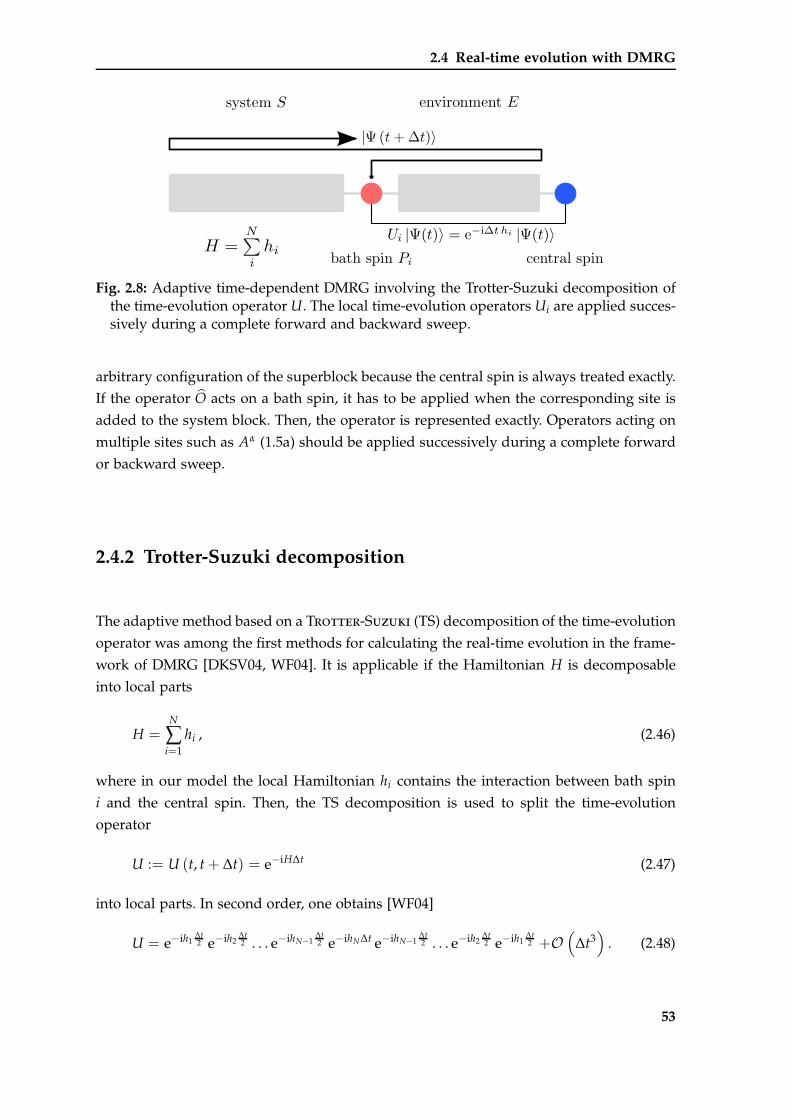
2.4 Real-time evolution with DMRG
Fig. 2.8: Adaptive time-dependent DMRG involving the Trotter-Suzuki decomposition ofthe time-evolution operator U. The local time-evolution operators Ui are applied succes-sively during a complete forward and backward sweep.
arbitrary configuration of the superblock because the central spin is always treated exactly.
If the operator O acts on a bath spin, it has to be applied when the corresponding site is
added to the system block. Then, the operator is represented exactly. Operators acting on
multiple sites such as Aα (1.5a) should be applied successively during a complete forward
or backward sweep.
2.4.2 Trotter-Suzuki decomposition
The adaptive method based on a Trotter-Suzuki (TS) decomposition of the time-evolution
operator was among the first methods for calculating the real-time evolution in the frame-
work of DMRG [DKSV04, WF04]. It is applicable if the Hamiltonian H is decomposable
into local parts
H =N
∑i=1
hi , (2.46)
where in our model the local Hamiltonian hi contains the interaction between bath spin
i and the central spin. Then, the TS decomposition is used to split the time-evolution
operator
U := U (t, t + ∆t) = e−iH∆t (2.47)
into local parts. In second order, one obtains [WF04]
U = e−ih1∆t2 e−ih2
∆t2 . . . e−ihN−1
∆t2 e−ihN∆t e−ihN−1
∆t2 . . . e−ih2
∆t2 e−ih1
∆t2 +O
(∆t3)
. (2.48)
53
Chapter 2 Density Matrix Renormalization Group
Thereby, all local time-evolution operators are applied successively to their correspond-
ing configuration of bath and central spin during the sweeps through the superblock, see
Fig. 2.8. During a complete backward and forward sweep, each bath spin is addressed
twice and the local time-evolution operator can be applied to the individual configura-
tion of bath and central spin without any additional error beyond the discarded weight.
Hence, the real-time time evolution of one or more states is calculated by running the
finite size algorithm (Sect. 2.2.2) and successively applying the local time-evolution op-
erators Ui = e− i hi∆t to update the target states. As usual, the basis is optimized in each
step by truncating with respect to the most important eigenstates of the reduced density
matrix. After two complete half-sweeps, the time evolution has proceeded by one interval
∆t. The desired quantities are measured and one continues to sweep until the maximum
time is reached. Changes have to be made only to the transformations of the state vector
described in Appendix A. An additional step is introduced after one has arrived at the
expression in Eq. (A.5) where both the central spin and the single bath spin are separated
from the superblock. This is represented by four different matrices Ψ, each of them corre-
sponding to one of the four configurations |σ0σi〉 ∈ |↑↑〉 , |↑↓〉 , |↓↑〉 , |↓↓〉 of central spin
and bath spin. Before one proceeds with the next step (A.6) of the transformation, these
four matrices are replaced by
Ψml ,mN−l−1,σ0,σi−→ Ui;σ0σi
Ψml ,mN−l−1,σ0,σi(2.49)
to calculate the time evolution of the local configuration. Here, the Ui;σ0σiare the matrix
elements of the local time-evolution operator Ui. When an auxiliary site is transformed, Ui
corresponds to the identity. Otherwise, the local parts Ui in Eq. (2.49) are 4 × 4 matrices.
They are either known exactly or they can be computed with small numerical effort.
The Trotter-Suzuki decomposition (2.48) is not exact and involves an error in addition to
the discarded weight. In second order, the Trotter-Suzuki error is ∼ ∆t3. As the decompo-
sition is applied tmax/∆t times, the total error accumulates to O(∆t2).
Higher orders of the Trotter-Suzuki decomposition reduce this error. The fourth order is
derived in Appendix B. Thereby, one step in the real-time evolution is performed with
three backward and forward sweeps and the Trotter-Suzuki error is of O(∆t5). Hence, the
error due to the decomposition is decreased upon two orders of magnitude by increasing
the run-time by a factor of three. However, it is not always necessary to use higher or-
ders of the decomposition. The Trotter-Suzuki error is almost constant so that it usually
dominates the total error only for small times. Generically, the discarded weight is the
limiting factor because it accumulates with increasing time. A more detailed discussion of
the Trotter-Suzuki error is presented in Sect. 2.6. The interested reader is also referred to
Ref. [GKSS05].
54
2.4 Real-time evolution with DMRG
2.4.3 Krylov vectors
The approach based on the Trotter-Suzuki decomposition takes advantage of the features
of the finite size algorithm in a very elegant way. But its application is restricted to Hamil-
tonians which can be decomposed according to Eq. (2.46). Furthermore, the Trotter-Suzuki
error occurs in addition to the discarded weight.
In this section, we follow a different strategy and discuss the direct application of the time-
evolution operator U to the state vector so that a decomposition is not required. As the
Hamiltonian of the superblock, the time-evolution operator U cannot be applied directly
to the superblock state. Thus, U has to be expanded in a well-defined basis. The idea be-
hind this approach is that first the basis is optimized for the time-interval t and t + ∆t.
This is done by targeting several states |Ψ(ti)〉 for ti ∈ [t, t + ∆t]. Usually, this procedure
converges fast and a few half sweeps are sufficient to optimize this basis. Afterwards, the
time evolution of the superblock state from t to t + ∆t is calculated. To reduce the integra-
tion error, it is possible to use smaller time steps for the evolution than for the calculation
of the target states. In a first approach discussed by Feiguin and White [FW05], a Runge-
Kutta integration was used to calculate the target states and the real-time evolution. But
they also suggested to employ other methods, for example a Lanczos tridiagonalization of
the Hamiltonian. In contrast to the Runge-Kutte integration, this approach preserves uni-
tarity. However, we have to keep in mind that unitarity is always violated by the DMRG
truncation of the Hilbert space.
Note that an alternative scheme for calculating the time evolution with DMRG based
on Krylov vectors was introduced by Schmitteckert [Sch04]. But instead of optimizing
the basis and performing the time evolution in the interval t and t + ∆t successively as
suggested later on by Feiguin and White [FW05], Schmitteckert carried out the complete
time evolution in each step of the algorithm.
In the following, we employ Krylov vectors [HL97, HL99, MMN05, NM05, Fri06, SRU13]
for the calculation of the target states as well as for the real-time evolution and stick to
the basis optimization proposed in Ref. [FW05]. Therefore, the state vector at t + ∆t is
expanded in the basis of the Krylov subspace
|Ψ (t)〉 , H |Ψ (t)〉 , H2 |Ψ (t)〉 , . . . , Hk−1 |Ψ (t)〉
. (2.50)
An orthogonal basis of this subspace is spanned by the so called Krylov vectors |vn〉 which
are obtained by orthogonalizing the vectors from Eq. (2.50) via the well-known Lanczos
tridiagonalization. The recursion relation is given by
|v0〉 = |Ψ (t)〉 (2.51a)
|vn+1〉 = H |vn〉 − αn |vn〉 − β2n |vn−1〉 , (2.51b)
55
Chapter 2 Density Matrix Renormalization Group
where the previous two Krylov vectors and the coefficients
αn =〈vn| H |vn〉〈vn|vn〉
(2.52a)
β2n =
〈vn|vn〉〈vn−1|vn−1〉
(2.52b)
enter. We consider a k-dimensional Krylov subspace, where k is a very small number O(10)
compared to the dimension of the Hilbert space. In the Krylov subspace, the Hamilto-
nian
Tk = V⊤k HVk (2.53)
is a tridiagonal matrix and can be diagonalized easily using standard numerical routines.
The matrix Vk contains all k Krylov vectors of the subspace as columns. The time-evolution
operator is now approximated in the Krylov subspace
|Ψ (t + ∆t)〉 ≈ Vk e−iTk∆t V⊤k |Ψ (t)〉 . (2.54)
Note that |Ψ(t)〉 = |v0〉 is a Krylov vector. Thus, all columns of the matrix Vk except the
first one are orthogonal to |Ψ(t)〉. The tridiagonal Hamiltonian Tk is diagonalized by an
orthogonal transformation Ok
e−iTk∆t = Ok e−iDk∆t O⊤k , (2.55)
where Dk is a diagonal matrix.
Concerning the implementation of the Krylov vectors within our DMRG code, it is advis-
able to rewrite |Ψ(t + ∆t)〉 = e− i H∆t |Ψ(t)〉 in bra-ket notation. By inserting several basis
sets in the latter expression, the real-time evolution from t → t + ∆t acquires the form
|Ψ (t + ∆t)〉 =k−1
∑i=0
ai |vi〉 (2.56)
with the coefficients
ai =k−1
∑j=0
〈vi|λj〉 e−iλj∆t 〈λj|Ψ (t)〉 . (2.57)
The eigenvectors |λj〉 and eigenvalues λj result from the diagonalization of Tk, which
has to be calculated in addition to the orthogonalized Krylov vectors |vj〉.
The coefficients ai decay extremely fast with increasing number k. Thus, the dimension k
of the Krylov subspace can be kept very small. The modulus of the coefficients can be used
56
2.4 Real-time evolution with DMRG
as convergence criterion. In practice, we omit contributions with |ak| < 10−10 and only a
handful of Krylov vectors is required.
The appropriate choice for the target states used for the basis optimization was intensively
discussed in Ref. [FW05]. In our realization, we stick to the established choice of four states
|Ψ1〉 = |Ψ(t)〉 , |Ψ2〉 = |Ψ(t + ∆t/3)〉 , |Ψ3〉 = |Ψ(t + 2∆t/3)〉 , |Ψ4〉 = |Ψ(t + ∆t)〉 .
(2.58a)
The weights of the target states in the reduced density matrix have only a minor influence
on the results. An overweight for the target states |Ψ(t)〉 and |Ψ(t + ∆t)〉 has proven to
yield a slightly better performance than equal weights. Thus, we adopt the weights
W1 =13
, W2 =16
, W3 =16
, W4 =13
(2.58b)
for the four target states (2.58a) from Feiguin and White [FW05].
Like the TS decomposition, the implementation of the Krylov vector approach is straight-
forward because the Lanczos algorithm occurs in many standard DMRG codes anyway.
The run-times are significantly longer compared to the previously introduced TS decom-
position, because the action of the Hamiltonian on the state vector has to be calculated
multiple times in each step. But it does not suffer from the error of the TS decomposition.
The action of the Hamiltonian on the state vectors is directly evaluated by applying all op-
erators contributing to the Hamiltonian, see Sect. 2.2.1. Thus, special care has to be taken
that all operators in a purified system are restricted to real sites only. The accuracy is well
controllable by adjusting the cutoff of the expansion coefficients ak (2.57).
2.4.4 Chebychev expansion
The Chebychev expansion [TEK84] is a widely known approach for calculating the time
evolution [DDR03, WWAF06, HA14]. More recently, it has also been implemented in the
framework of matrix product states in combination with a variational calculation of the
Chebychev polynomials [HWM+11]. In the following, we present how we use the Cheby-
chev expansion to calculate the real-time evolution of autocorrelation functions with a
standard DMRG implementation [SRU13].
To this end, we return to the concept of purification as introduced in Sect. 2.3.2 and con-
sider the initial state
|0〉 :=N⊗
i=0
1√2
(|↑r↓a〉 − |↓r↑a〉
)i, (2.59)
57
Chapter 2 Density Matrix Renormalization Group
where the central spin is purified as well. This setup is sketched in the lower panel of
Fig. 2.7. Since all operators are restricted to real sites, it is possible to apply any unitary
operator to the auxiliary sites without affecting the physics of the model. Hence, an arti-
ficial time evolution of the auxiliary sites is realizable. We follow the proposal made by
Karrasch et al. [KBM12]. They studied a purified Heisenberg chain and used the same
Hamiltonian for the auxiliary spins but calculated their real-time evolution backwards in
time. In the Heisenberg chain, this leads to a slower growth of the entanglement and thus
to a slower increase of the discarded weight.
Due to the purified central site in the initial state |0〉, we are able to adopt this approach
for the central spin model. We consider an autocorrelation function of the central spin in
the Heisenberg picture, for example in z-direction,
S (t) = 〈0|U† (t) Sz0U (t) Sz
0|0〉 , (2.60)
where U(t) = e−itH with H = Hr − Ha acts on the real and the auxiliary spins. The
Hamiltonian Hr represents the standard Hamiltonian (1.4) of the central spin model and
acts on the real spins only. The auxiliary Hamiltonian Ha involves the same interactions
as Hr, but it is solely restricted to the auxiliary spins. As the real spins evolve forward
and the auxiliary spins evolve backward in time, the action of U(†) on |0〉 leaves this state
unchanged. This observation is the reason for the reduced growth of entanglement in chain
topologies. For a more detailed discussion, see Appendix C. Thus, the autocorrelation
function (2.60) acquires the symmetric form
S (t) = 〈0|Sz0U (t) Sz
0|0〉 . (2.61)
This is crucial for the Chebychev expansion, which we see below.
Concerning the application of the Chebychev polynomials, the Hamiltonian has to be
rescaled with the energy bound C = 3/4 ∑Ni=1 |Ji| to ensure the validity of the expansion.
The correct estimate for C is yield from the maximum energy of the Hamiltonian. The
energy of a single dimer formed by the bath spin ~Si and the central spin ~S0 is bounded
by |Ji~Si~S0| ≤ 3|Ji|/4, which corresponds to the energy of an antiferromagnetic dimer.
By summing over all dimers, one obtains the previously mentioned expression for C.
An additional factor of two is induced by the auxiliary Hamiltonian Ha, which has the
same energy bound. Hence, the eigenvalues of the rescaled Hamiltonian H = H/(2C)
fulfill −1 ≤ En ≤ 1. The time-evolution operator U is now expanded in the basis of the
Chebychev polynomials Tchn (H)
e−iHt =∞
∑n=0
Tchn
(Hr − Ha
2C
)bn (2Ct) . (2.62)
58
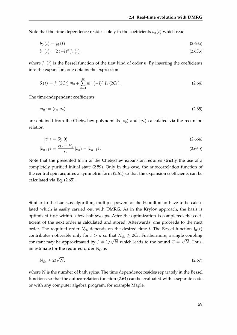
2.4 Real-time evolution with DMRG
Note that the time dependence resides solely in the coefficients bn(t) which read
b0 (t) = J0 (t) (2.63a)
bn (t) = 2 (−i)n Jn (t) , (2.63b)
where Jn (t) is the Bessel function of the first kind of order n. By inserting the coefficients
into the expansion, one obtains the expression
S (t) = J0 (2Ct) m0 +∞
∑n=1
mn (−i)n Jn (2Ct) . (2.64)
The time-independent coefficients
mn := 〈v0|vn〉 (2.65)
are obtained from the Chebychev polynomials |v0〉 and |vn〉 calculated via the recursion
relation
|v0〉 = Sz0 |0〉 (2.66a)
|vn+1〉 =Hr − Ha
C|vn〉 − |vn−1〉 . (2.66b)
Note that the presented form of the Chebychev expansion requires strictly the use of a
completely purified initial state (2.59). Only in this case, the autocorrelation function of
the central spin acquires a symmetric form (2.61) so that the expansion coefficients can be
calculated via Eq. (2.65).
Similar to the Lanczos algorithm, multiple powers of the Hamiltonian have to be calcu-
lated which is easily carried out with DMRG. As in the Krylov approach, the basis is
optimized first within a few half-sweeps. After the optimization is completed, the coef-
ficient of the next order is calculated and stored. Afterwards, one proceeds to the next
order. The required order Nch depends on the desired time t. The Bessel function Jn(t)
contributes noticeable only for t > n so that Nch ≥ 2Ct. Furthermore, a single coupling
constant may be approximated by J ≈ 1/√
N which leads to the bound C =√
N. Thus,
an estimate for the required order Nch is
Nch ≥ 2t√
N, (2.67)
where N is the number of bath spins. The time dependence resides separately in the Bessel
functions so that the autocorrelation function (2.64) can be evaluated with a separate code
or with any computer algebra program, for example Maple.
59
Chapter 2 Density Matrix Renormalization Group
In the reduced density matrix, at least the four states |v0〉 , |vn−1〉 , |vn〉, and |vn+1〉 have
to be targeted. The targeting of the initial state |v0〉 is crucial because it is required for
the calculation of the coefficients mn (2.65). Thereby, one ensures that the basis of |v0〉 is
always ideally represented. If the target state is missing, errors will occur which lead to
false coefficients mn. However, the state |0〉 has a very simple structure so that there is no
negative effect on the discarded weight when it is targeted in addition to the latest three
Chebychev polynomials.
With respect to the special role of |v0〉, one also has to be careful about its normalization.
If the state |v0〉 is transformed over and over again, its normalization will be lost after
multiple sweeps, see Sect. 2.5.2.2 for details. To prevent this, we recommend to rebuild the
state in each recursion step which can be done during a half-sweep. This strongly reduces
the error of the Chebychev polynomials mn. All others states are only stored for three
orders and no recalculation is necessary.
Compared to a Trotter-Suzuki or Krylov calculation, the size of the Hilbert space is dou-
bled due to the purified central site. This leads to an increase of the runtime. But for a
fixed value of t, it is much faster than the Krylov vector approach because the required or-
der for the Chebychev expansion involves significantly less applications of the superblock
Hamiltonian. An additional speed-up is obtained by outsourcing the calculation of the
autocorrelation function (2.64). In total, the required run-time of the Chebychev code is
moderate and ranks between the Trotter-Suzuki and Krylov approach, see Sect. 2.5.4 for
details.
2.5 Verification of the DMRG implementation
The ground state energies presented in Sect. 2.2.2 already revealed a remarkable agree-
ment between DMRG and the exact results. Before we start with a detailed discussion of
the central spin dynamics in the central spin model, the implementation of the real-time
evolution based on DMRG has to be verified.
2.5.1 Polarized bath
For the beginning, it is convenient to study a simple initial state where the exact time
evolution is known. We discuss a fully polarized bath with all bath spins pointing up and
60
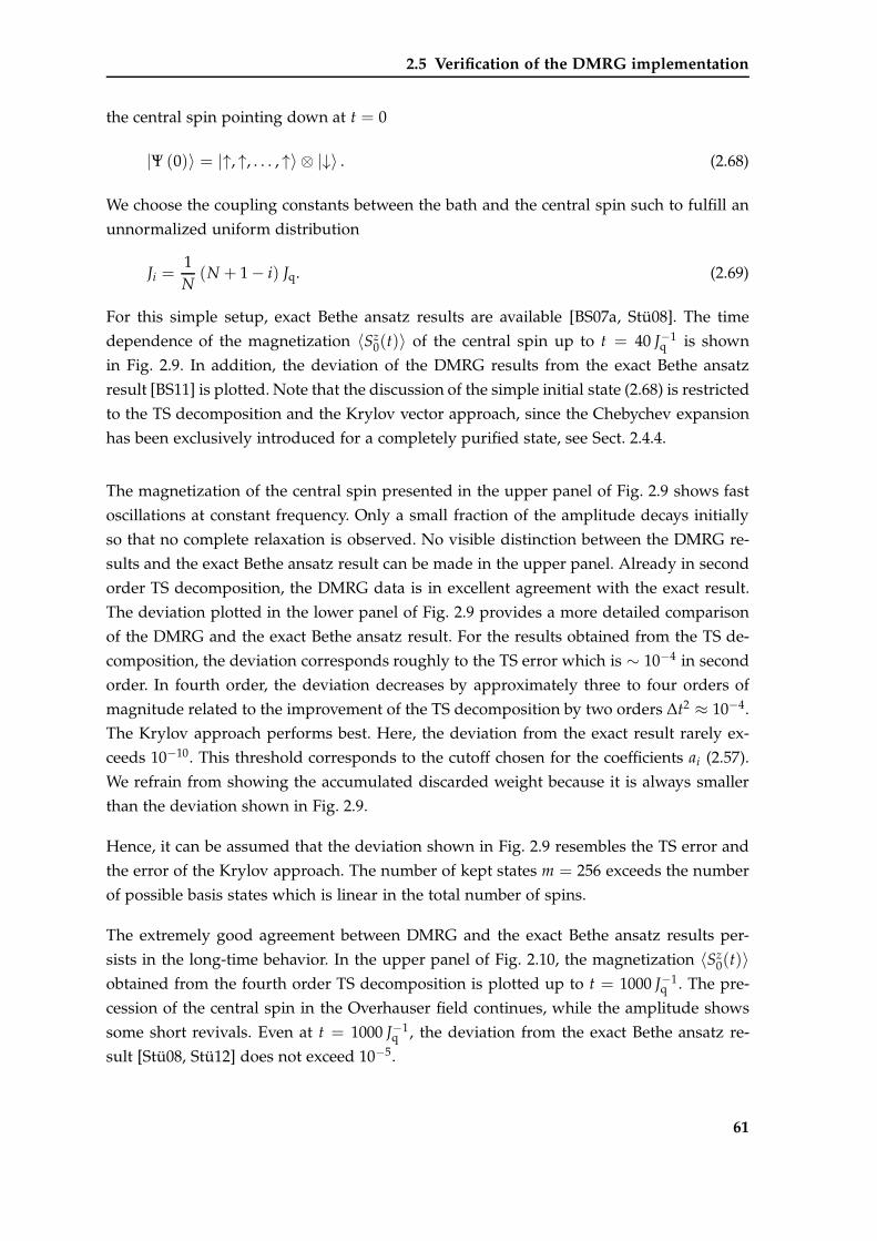
2.5 Verification of the DMRG implementation
the central spin pointing down at t = 0
|Ψ (0)〉 = |↑, ↑, . . . , ↑〉 ⊗ |↓〉 . (2.68)
We choose the coupling constants between the bath and the central spin such to fulfill an
unnormalized uniform distribution
Ji =1N
(N + 1 − i) Jq. (2.69)
For this simple setup, exact Bethe ansatz results are available [BS07a, Stü08]. The time
dependence of the magnetization 〈Sz0(t)〉 of the central spin up to t = 40 J−1
q is shown
in Fig. 2.9. In addition, the deviation of the DMRG results from the exact Bethe ansatz
result [BS11] is plotted. Note that the discussion of the simple initial state (2.68) is restricted
to the TS decomposition and the Krylov vector approach, since the Chebychev expansion
has been exclusively introduced for a completely purified state, see Sect. 2.4.4.
The magnetization of the central spin presented in the upper panel of Fig. 2.9 shows fast
oscillations at constant frequency. Only a small fraction of the amplitude decays initially
so that no complete relaxation is observed. No visible distinction between the DMRG re-
sults and the exact Bethe ansatz result can be made in the upper panel. Already in second
order TS decomposition, the DMRG data is in excellent agreement with the exact result.
The deviation plotted in the lower panel of Fig. 2.9 provides a more detailed comparison
of the DMRG and the exact Bethe ansatz result. For the results obtained from the TS de-
composition, the deviation corresponds roughly to the TS error which is ∼ 10−4 in second
order. In fourth order, the deviation decreases by approximately three to four orders of
magnitude related to the improvement of the TS decomposition by two orders ∆t2 ≈ 10−4.
The Krylov approach performs best. Here, the deviation from the exact result rarely ex-
ceeds 10−10. This threshold corresponds to the cutoff chosen for the coefficients ai (2.57).
We refrain from showing the accumulated discarded weight because it is always smaller
than the deviation shown in Fig. 2.9.
Hence, it can be assumed that the deviation shown in Fig. 2.9 resembles the TS error and
the error of the Krylov approach. The number of kept states m = 256 exceeds the number
of possible basis states which is linear in the total number of spins.
The extremely good agreement between DMRG and the exact Bethe ansatz results per-
sists in the long-time behavior. In the upper panel of Fig. 2.10, the magnetization 〈Sz0(t)〉
obtained from the fourth order TS decomposition is plotted up to t = 1000 J−1q . The pre-
cession of the central spin in the Overhauser field continues, while the amplitude shows
some short revivals. Even at t = 1000 J−1q , the deviation from the exact Bethe ansatz re-
sult [Stü08, Stü12] does not exceed 10−5.
61
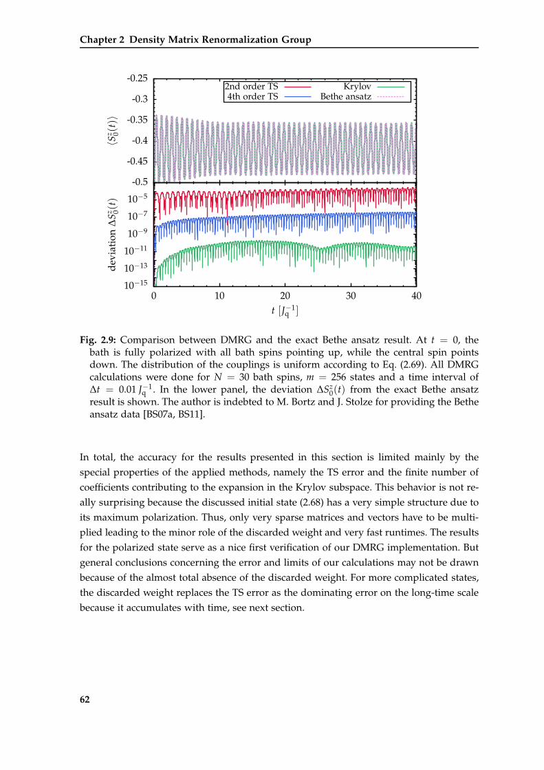
Chapter 2 Density Matrix Renormalization Group
-0.5
-0.45
-0.4
-0.35
-0.3
-0.25
〈Sz 0(
t)〉
10−15
10−13
10−11
10−9
10−7
10−5
0 10 20 30 40
dev
iati
on∆
Sz 0(
t)
t [J−1q ]
2nd order TS4th order TS
KrylovBethe ansatz
Fig. 2.9: Comparison between DMRG and the exact Bethe ansatz result. At t = 0, thebath is fully polarized with all bath spins pointing up, while the central spin pointsdown. The distribution of the couplings is uniform according to Eq. (2.69). All DMRGcalculations were done for N = 30 bath spins, m = 256 states and a time interval of∆t = 0.01 J−1
q . In the lower panel, the deviation ∆Sz0(t) from the exact Bethe ansatz
result is shown. The author is indebted to M. Bortz and J. Stolze for providing the Betheansatz data [BS07a, BS11].
In total, the accuracy for the results presented in this section is limited mainly by the
special properties of the applied methods, namely the TS error and the finite number of
coefficients contributing to the expansion in the Krylov subspace. This behavior is not re-
ally surprising because the discussed initial state (2.68) has a very simple structure due to
its maximum polarization. Thus, only very sparse matrices and vectors have to be multi-
plied leading to the minor role of the discarded weight and very fast runtimes. The results
for the polarized state serve as a nice first verification of our DMRG implementation. But
general conclusions concerning the error and limits of our calculations may not be drawn
because of the almost total absence of the discarded weight. For more complicated states,
the discarded weight replaces the TS error as the dominating error on the long-time scale
because it accumulates with time, see next section.
62
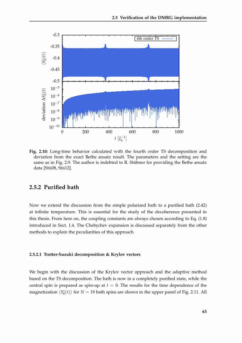
2.5 Verification of the DMRG implementation
-0.5
-0.45
-0.4
-0.35
-0.3
〈Sz 0(
t)〉
10−10
10−9
10−8
10−7
10−6
10−5
0 200 400 600 800 1000
dev
iati
on∆
Sz 0(
t)
t [J−1q ]
4th order TS
Fig. 2.10: Long-time behavior calculated with the fourth order TS decomposition anddeviation from the exact Bethe ansatz result. The parameters and the setting are thesame as in Fig. 2.9. The author is indebted to R. Stübner for providing the Bethe ansatzdata [Stü08, Stü12].
2.5.2 Purified bath
Now we extend the discussion from the simple polarized bath to a purified bath (2.42)
at infinite temperature. This is essential for the study of the decoherence presented in
this thesis. From here on, the coupling constants are always chosen according to Eq. (1.8)
introduced in Sect. 1.4. The Chebychev expansion is discussed separately from the other
methods to explain the peculiarities of this approach.
2.5.2.1 Trotter-Suzuki decomposition & Krylov vectors
We begin with the discussion of the Krylov vector approach and the adaptive method
based on the TS decomposition. The bath is now in a completely purified state, while the
central spin is prepared as spin-up at t = 0. The results for the time dependence of the
magnetization 〈Sz0(t)〉 for N = 19 bath spins are shown in the upper panel of Fig. 2.11. All
63
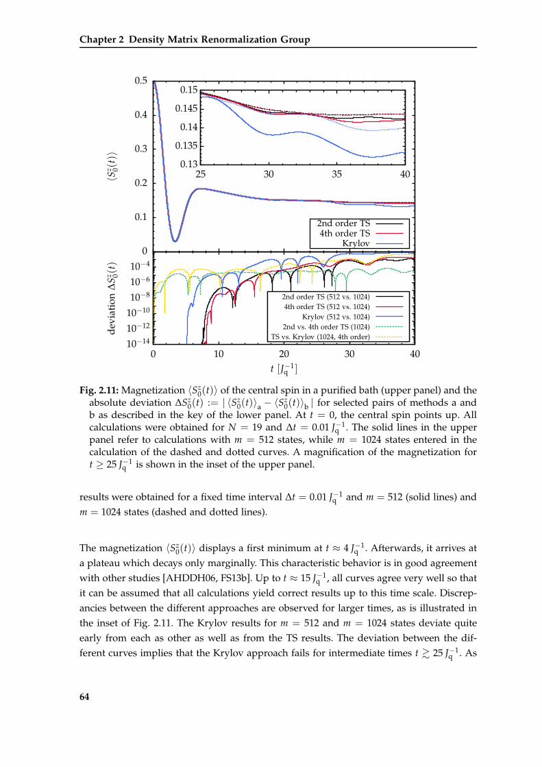
Chapter 2 Density Matrix Renormalization Group
0
0.1
0.2
0.3
0.4
0.5
〈Sz 0(
t)〉
0.13
0.135
0.14
0.145
0.15
25 30 35 40
10−14
10−12
10−10
10−8
10−6
10−4
0 10 20 30 40
dev
iati
on∆
Sz 0(
t)
t [J−1q ]
2nd order TS4th order TS
Krylov
2nd order TS (512 vs. 1024)4th order TS (512 vs. 1024)
Krylov (512 vs. 1024)2nd vs. 4th order TS (1024)
TS vs. Krylov (1024, 4th order)
Fig. 2.11: Magnetization 〈Sz0(t)〉 of the central spin in a purified bath (upper panel) and the
absolute deviation ∆Sz0(t) := | 〈Sz
0(t)〉a − 〈Sz0(t)〉b | for selected pairs of methods a and
b as described in the key of the lower panel. At t = 0, the central spin points up. Allcalculations were obtained for N = 19 and ∆t = 0.01 J−1
q . The solid lines in the upperpanel refer to calculations with m = 512 states, while m = 1024 states entered in thecalculation of the dashed and dotted curves. A magnification of the magnetization fort ≥ 25 J−1
q is shown in the inset of the upper panel.
results were obtained for a fixed time interval ∆t = 0.01 J−1q and m = 512 (solid lines) and
m = 1024 states (dashed and dotted lines).
The magnetization 〈Sz0(t)〉 displays a first minimum at t ≈ 4 J−1
q . Afterwards, it arrives at
a plateau which decays only marginally. This characteristic behavior is in good agreement
with other studies [AHDDH06, FS13b]. Up to t ≈ 15 J−1q , all curves agree very well so that
it can be assumed that all calculations yield correct results up to this time scale. Discrep-
ancies between the different approaches are observed for larger times, as is illustrated in
the inset of Fig. 2.11. The Krylov results for m = 512 and m = 1024 states deviate quite
early from each as other as well as from the TS results. The deviation between the dif-
ferent curves implies that the Krylov approach fails for intermediate times t & 25 J−1q . As
64
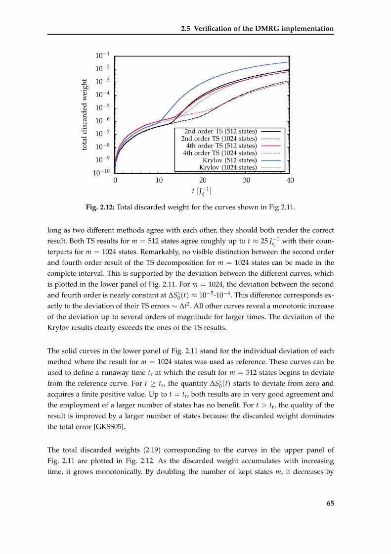
2.5 Verification of the DMRG implementation
10−10
10−9
10−8
10−7
10−6
10−5
10−4
10−3
10−2
10−1
0 10 20 30 40
tota
ldis
card
edw
eigh
t
t [J−1q ]
2nd order TS (512 states)2nd order TS (1024 states)
4th order TS (512 states)4th order TS (1024 states)
Krylov (512 states)Krylov (1024 states)
Fig. 2.12: Total discarded weight for the curves shown in Fig 2.11.
long as two different methods agree with each other, they should both render the correct
result. Both TS results for m = 512 states agree roughly up to t ≈ 25 J−1q with their coun-
terparts for m = 1024 states. Remarkably, no visible distinction between the second order
and fourth order result of the TS decomposition for m = 1024 states can be made in the
complete interval. This is supported by the deviation between the different curves, which
is plotted in the lower panel of Fig. 2.11. For m = 1024, the deviation between the second
and fourth order is nearly constant at ∆Sz0(t) ≈ 10−5-10−4. This difference corresponds ex-
actly to the deviation of their TS errors ∼ ∆t2. All other curves reveal a monotonic increase
of the deviation up to several orders of magnitude for larger times. The deviation of the
Krylov results clearly exceeds the ones of the TS results.
The solid curves in the lower panel of Fig. 2.11 stand for the individual deviation of each
method where the result for m = 1024 states was used as reference. These curves can be
used to define a runaway time tr at which the result for m = 512 states begins to deviate
from the reference curve. For t ≥ tr, the quantity ∆Sz0(t) starts to deviate from zero and
acquires a finite positive value. Up to t = tr, both results are in very good agreement and
the employment of a larger number of states has no benefit. For t > tr, the quality of the
result is improved by a larger number of states because the discarded weight dominates
the total error [GKSS05].
The total discarded weights (2.19) corresponding to the curves in the upper panel of
Fig. 2.11 are plotted in Fig. 2.12. As the discarded weight accumulates with increasing
time, it grows monotonically. By doubling the number of kept states m, it decreases by
65
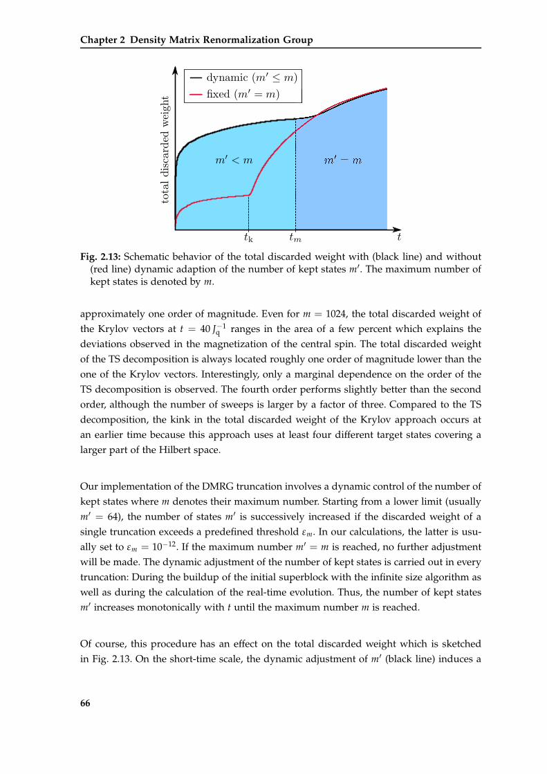
Chapter 2 Density Matrix Renormalization Group
Fig. 2.13: Schematic behavior of the total discarded weight with (black line) and without(red line) dynamic adaption of the number of kept states m′. The maximum number ofkept states is denoted by m.
approximately one order of magnitude. Even for m = 1024, the total discarded weight of
the Krylov vectors at t = 40 J−1q ranges in the area of a few percent which explains the
deviations observed in the magnetization of the central spin. The total discarded weight
of the TS decomposition is always located roughly one order of magnitude lower than the
one of the Krylov vectors. Interestingly, only a marginal dependence on the order of the
TS decomposition is observed. The fourth order performs slightly better than the second
order, although the number of sweeps is larger by a factor of three. Compared to the TS
decomposition, the kink in the total discarded weight of the Krylov approach occurs at
an earlier time because this approach uses at least four different target states covering a
larger part of the Hilbert space.
Our implementation of the DMRG truncation involves a dynamic control of the number of
kept states where m denotes their maximum number. Starting from a lower limit (usually
m′ = 64), the number of states m′ is successively increased if the discarded weight of a
single truncation exceeds a predefined threshold εm. In our calculations, the latter is usu-
ally set to εm = 10−12. If the maximum number m′ = m is reached, no further adjustment
will be made. The dynamic adjustment of the number of kept states is carried out in every
truncation: During the buildup of the initial superblock with the infinite size algorithm as
well as during the calculation of the real-time evolution. Thus, the number of kept states
m′ increases monotonically with t until the maximum number m is reached.
Of course, this procedure has an effect on the total discarded weight which is sketched
in Fig. 2.13. On the short-time scale, the dynamic adjustment of m′ (black line) induces a
66
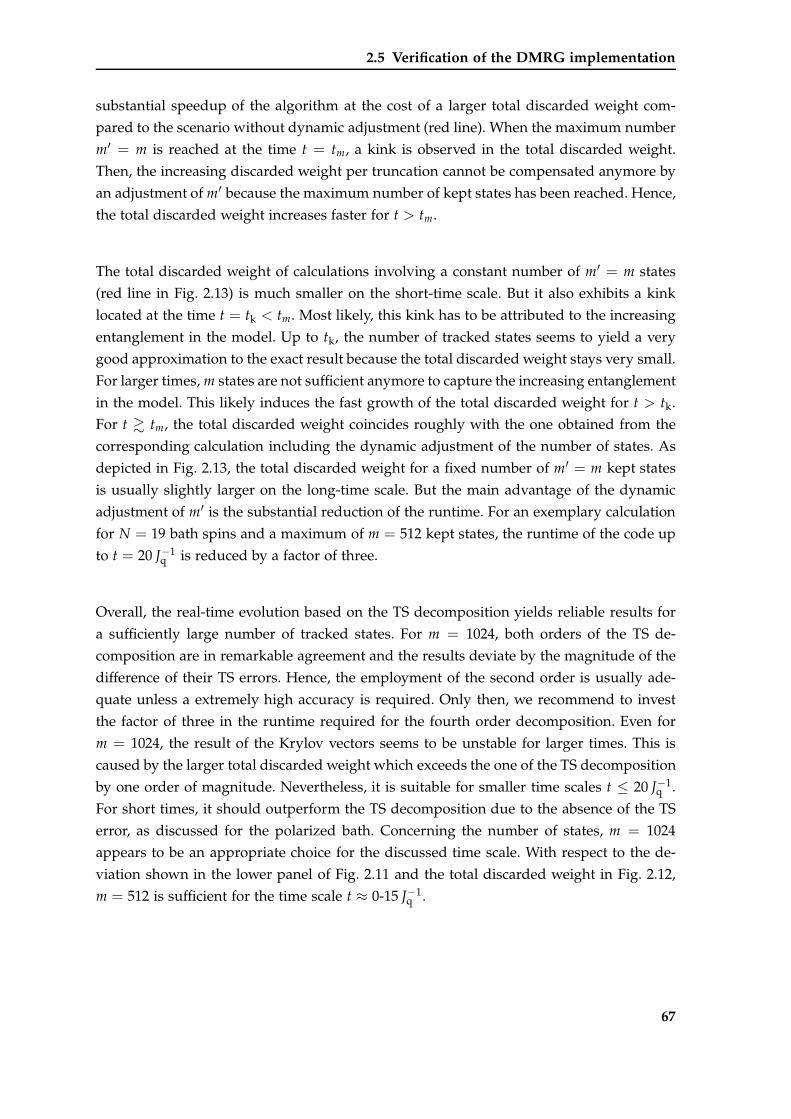
2.5 Verification of the DMRG implementation
substantial speedup of the algorithm at the cost of a larger total discarded weight com-
pared to the scenario without dynamic adjustment (red line). When the maximum number
m′ = m is reached at the time t = tm, a kink is observed in the total discarded weight.
Then, the increasing discarded weight per truncation cannot be compensated anymore by
an adjustment of m′ because the maximum number of kept states has been reached. Hence,
the total discarded weight increases faster for t > tm.
The total discarded weight of calculations involving a constant number of m′ = m states
(red line in Fig. 2.13) is much smaller on the short-time scale. But it also exhibits a kink
located at the time t = tk < tm. Most likely, this kink has to be attributed to the increasing
entanglement in the model. Up to tk, the number of tracked states seems to yield a very
good approximation to the exact result because the total discarded weight stays very small.
For larger times, m states are not sufficient anymore to capture the increasing entanglement
in the model. This likely induces the fast growth of the total discarded weight for t > tk.
For t & tm, the total discarded weight coincides roughly with the one obtained from the
corresponding calculation including the dynamic adjustment of the number of states. As
depicted in Fig. 2.13, the total discarded weight for a fixed number of m′ = m kept states
is usually slightly larger on the long-time scale. But the main advantage of the dynamic
adjustment of m′ is the substantial reduction of the runtime. For an exemplary calculation
for N = 19 bath spins and a maximum of m = 512 kept states, the runtime of the code up
to t = 20 J−1q is reduced by a factor of three.
Overall, the real-time evolution based on the TS decomposition yields reliable results for
a sufficiently large number of tracked states. For m = 1024, both orders of the TS de-
composition are in remarkable agreement and the results deviate by the magnitude of the
difference of their TS errors. Hence, the employment of the second order is usually ade-
quate unless a extremely high accuracy is required. Only then, we recommend to invest
the factor of three in the runtime required for the fourth order decomposition. Even for
m = 1024, the result of the Krylov vectors seems to be unstable for larger times. This is
caused by the larger total discarded weight which exceeds the one of the TS decomposition
by one order of magnitude. Nevertheless, it is suitable for smaller time scales t ≤ 20 J−1q .
For short times, it should outperform the TS decomposition due to the absence of the TS
error, as discussed for the polarized bath. Concerning the number of states, m = 1024
appears to be an appropriate choice for the discussed time scale. With respect to the de-
viation shown in the lower panel of Fig. 2.11 and the total discarded weight in Fig. 2.12,
m = 512 is sufficient for the time scale t ≈ 0-15 J−1q .
67
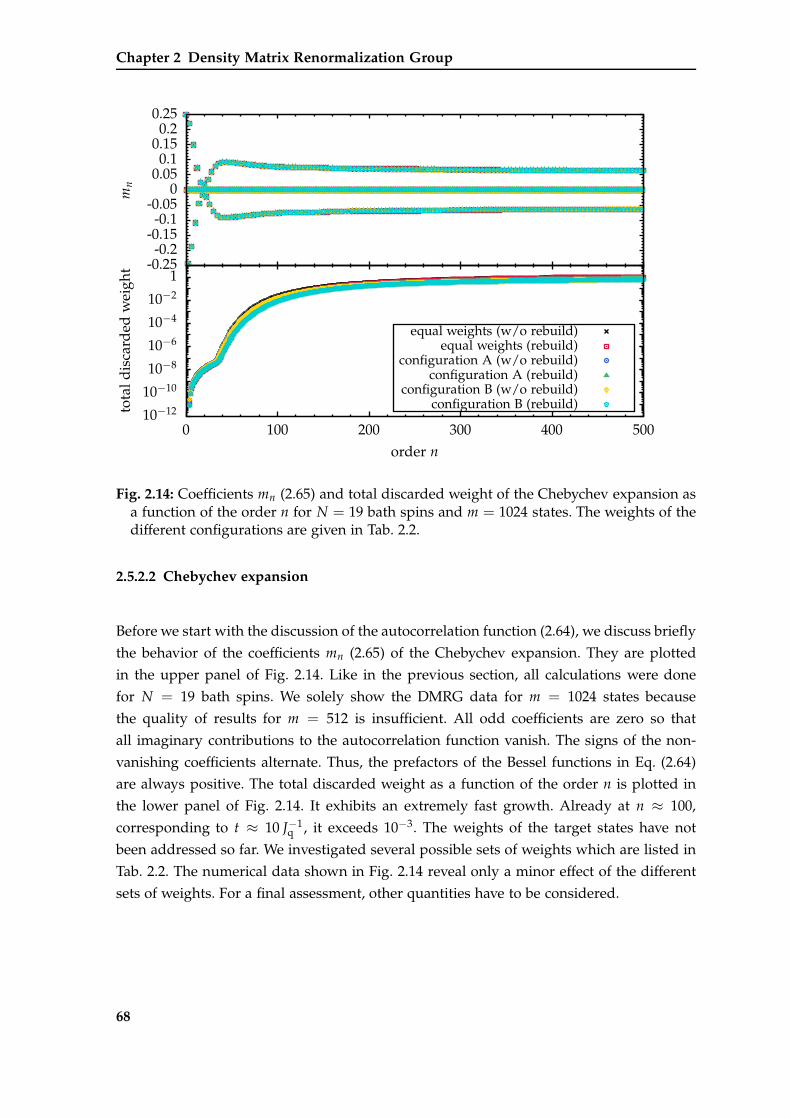
Chapter 2 Density Matrix Renormalization Group
-0.25-0.2
-0.15-0.1
-0.050
0.050.1
0.150.2
0.25m
n
10−12
10−10
10−8
10−6
10−4
10−2
1
0 100 200 300 400 500
tota
ldis
card
edw
eigh
t
order n
equal weights (w/o rebuild)equal weights (rebuild)
configuration A (w/o rebuild)configuration A (rebuild)
configuration B (w/o rebuild)configuration B (rebuild)
Fig. 2.14: Coefficients mn (2.65) and total discarded weight of the Chebychev expansion asa function of the order n for N = 19 bath spins and m = 1024 states. The weights of thedifferent configurations are given in Tab. 2.2.
2.5.2.2 Chebychev expansion
Before we start with the discussion of the autocorrelation function (2.64), we discuss briefly
the behavior of the coefficients mn (2.65) of the Chebychev expansion. They are plotted
in the upper panel of Fig. 2.14. Like in the previous section, all calculations were done
for N = 19 bath spins. We solely show the DMRG data for m = 1024 states because
the quality of results for m = 512 is insufficient. All odd coefficients are zero so that
all imaginary contributions to the autocorrelation function vanish. The signs of the non-
vanishing coefficients alternate. Thus, the prefactors of the Bessel functions in Eq. (2.64)
are always positive. The total discarded weight as a function of the order n is plotted in
the lower panel of Fig. 2.14. It exhibits an extremely fast growth. Already at n ≈ 100,
corresponding to t ≈ 10 J−1q , it exceeds 10−3. The weights of the target states have not
been addressed so far. We investigated several possible sets of weights which are listed in
Tab. 2.2. The numerical data shown in Fig. 2.14 reveal only a minor effect of the different
sets of weights. For a final assessment, other quantities have to be considered.
68
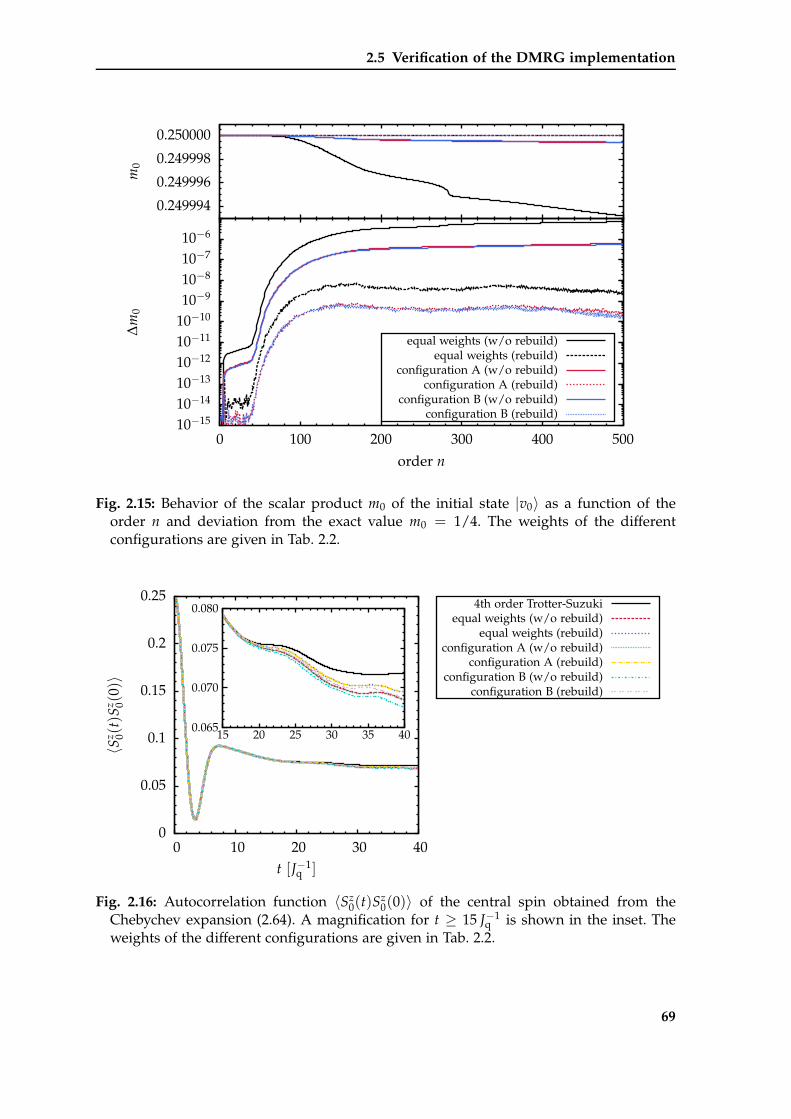
2.5 Verification of the DMRG implementation
0.249994
0.249996
0.249998
0.250000m
0
10−1510−1410−1310−1210−1110−1010−910−810−710−6
0 100 200 300 400 500
∆m
0
order n
equal weights (w/o rebuild)equal weights (rebuild)
configuration A (w/o rebuild)configuration A (rebuild)
configuration B (w/o rebuild)configuration B (rebuild)
Fig. 2.15: Behavior of the scalar product m0 of the initial state |v0〉 as a function of theorder n and deviation from the exact value m0 = 1/4. The weights of the differentconfigurations are given in Tab. 2.2.
0
0.05
0.1
0.15
0.2
0.25
0 10 20 30 40
〈Sz 0(
t)S
z 0(0)〉
t [J−1q ]
0.065
0.070
0.075
0.080
15 20 25 30 35 40
4th order Trotter-Suzukiequal weights (w/o rebuild)
equal weights (rebuild)configuration A (w/o rebuild)
configuration A (rebuild)configuration B (w/o rebuild)
configuration B (rebuild)
Fig. 2.16: Autocorrelation function 〈Sz0(t)S
z0(0)〉 of the central spin obtained from the
Chebychev expansion (2.64). A magnification for t ≥ 15 J−1q is shown in the inset. The
weights of the different configurations are given in Tab. 2.2.
69
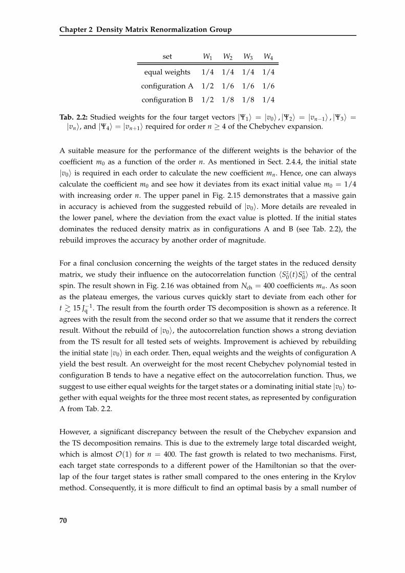
Chapter 2 Density Matrix Renormalization Group
set W1 W2 W3 W4
equal weights 1/4 1/4 1/4 1/4
configuration A 1/2 1/6 1/6 1/6
configuration B 1/2 1/8 1/8 1/4
Tab. 2.2: Studied weights for the four target vectors |Ψ1〉 = |v0〉 , |Ψ2〉 = |vn−1〉 , |Ψ3〉 =|vn〉, and |Ψ4〉 = |vn+1〉 required for order n ≥ 4 of the Chebychev expansion.
A suitable measure for the performance of the different weights is the behavior of the
coefficient m0 as a function of the order n. As mentioned in Sect. 2.4.4, the initial state
|v0〉 is required in each order to calculate the new coefficient mn. Hence, one can always
calculate the coefficient m0 and see how it deviates from its exact initial value m0 = 1/4
with increasing order n. The upper panel in Fig. 2.15 demonstrates that a massive gain
in accuracy is achieved from the suggested rebuild of |v0〉. More details are revealed in
the lower panel, where the deviation from the exact value is plotted. If the initial states
dominates the reduced density matrix as in configurations A and B (see Tab. 2.2), the
rebuild improves the accuracy by another order of magnitude.
For a final conclusion concerning the weights of the target states in the reduced density
matrix, we study their influence on the autocorrelation function 〈Sz0(t)S
z0〉 of the central
spin. The result shown in Fig. 2.16 was obtained from Nch = 400 coefficients mn. As soon
as the plateau emerges, the various curves quickly start to deviate from each other for
t & 15 J−1q . The result from the fourth order TS decomposition is shown as a reference. It
agrees with the result from the second order so that we assume that it renders the correct
result. Without the rebuild of |v0〉, the autocorrelation function shows a strong deviation
from the TS result for all tested sets of weights. Improvement is achieved by rebuilding
the initial state |v0〉 in each order. Then, equal weights and the weights of configuration A
yield the best result. An overweight for the most recent Chebychev polynomial tested in
configuration B tends to have a negative effect on the autocorrelation function. Thus, we
suggest to use either equal weights for the target states or a dominating initial state |v0〉 to-
gether with equal weights for the three most recent states, as represented by configuration
A from Tab. 2.2.
However, a significant discrepancy between the result of the Chebychev expansion and
the TS decomposition remains. This is due to the extremely large total discarded weight,
which is almost O(1) for n = 400. The fast growth is related to two mechanisms. First,
each target state corresponds to a different power of the Hamiltonian so that the over-
lap of the four target states is rather small compared to the ones entering in the Krylov
method. Consequently, it is more difficult to find an optimal basis by a small number of
70
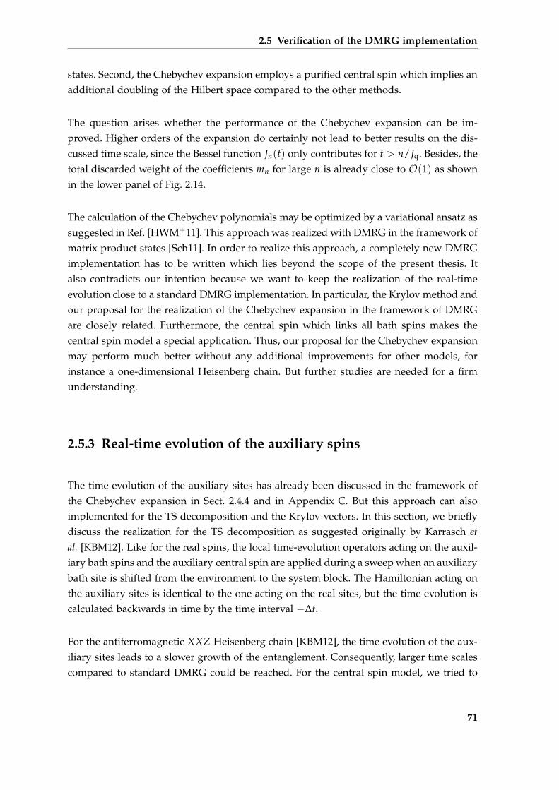
2.5 Verification of the DMRG implementation
states. Second, the Chebychev expansion employs a purified central spin which implies an
additional doubling of the Hilbert space compared to the other methods.
The question arises whether the performance of the Chebychev expansion can be im-
proved. Higher orders of the expansion do certainly not lead to better results on the dis-
cussed time scale, since the Bessel function Jn(t) only contributes for t > n/Jq. Besides, the
total discarded weight of the coefficients mn for large n is already close to O(1) as shown
in the lower panel of Fig. 2.14.
The calculation of the Chebychev polynomials may be optimized by a variational ansatz as
suggested in Ref. [HWM+11]. This approach was realized with DMRG in the framework of
matrix product states [Sch11]. In order to realize this approach, a completely new DMRG
implementation has to be written which lies beyond the scope of the present thesis. It
also contradicts our intention because we want to keep the realization of the real-time
evolution close to a standard DMRG implementation. In particular, the Krylov method and
our proposal for the realization of the Chebychev expansion in the framework of DMRG
are closely related. Furthermore, the central spin which links all bath spins makes the
central spin model a special application. Thus, our proposal for the Chebychev expansion
may perform much better without any additional improvements for other models, for
instance a one-dimensional Heisenberg chain. But further studies are needed for a firm
understanding.
2.5.3 Real-time evolution of the auxiliary spins
The time evolution of the auxiliary sites has already been discussed in the framework of
the Chebychev expansion in Sect. 2.4.4 and in Appendix C. But this approach can also
implemented for the TS decomposition and the Krylov vectors. In this section, we briefly
discuss the realization for the TS decomposition as suggested originally by Karrasch et
al. [KBM12]. Like for the real spins, the local time-evolution operators acting on the auxil-
iary bath spins and the auxiliary central spin are applied during a sweep when an auxiliary
bath site is shifted from the environment to the system block. The Hamiltonian acting on
the auxiliary sites is identical to the one acting on the real sites, but the time evolution is
calculated backwards in time by the time interval −∆t.
For the antiferromagnetic XXZ Heisenberg chain [KBM12], the time evolution of the aux-
iliary sites leads to a slower growth of the entanglement. Consequently, larger time scales
compared to standard DMRG could be reached. For the central spin model, we tried to
71
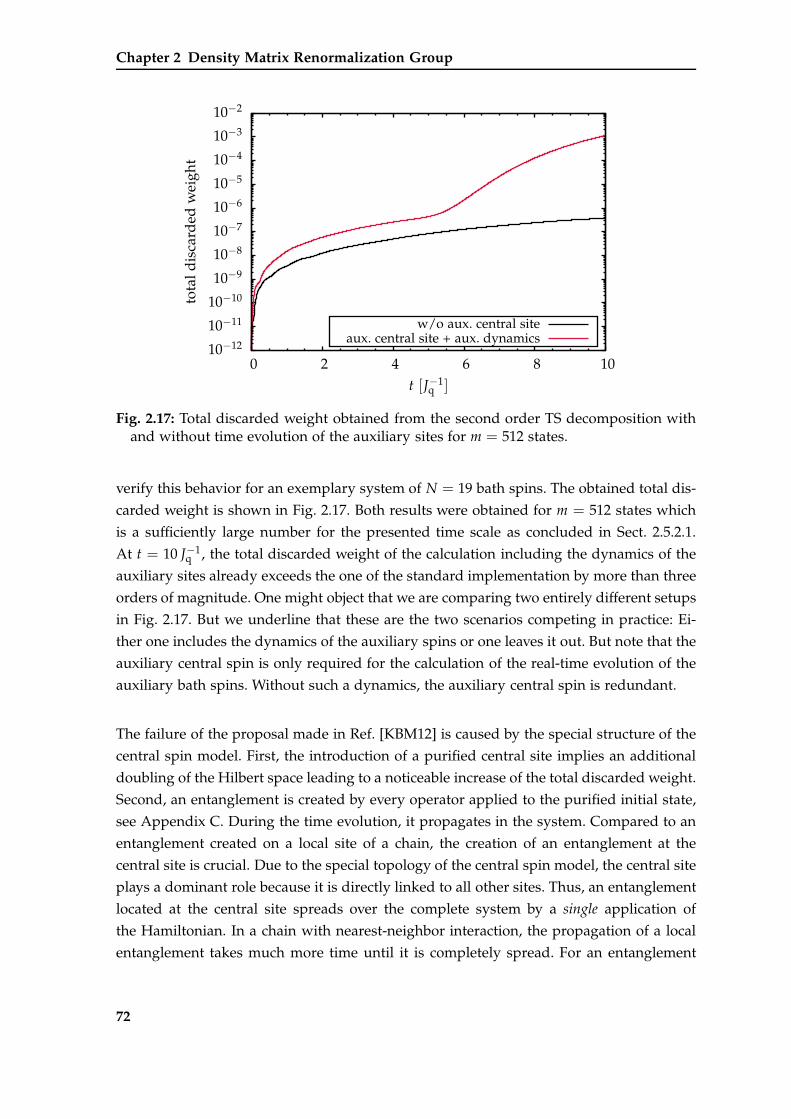
Chapter 2 Density Matrix Renormalization Group
10−12
10−11
10−10
10−9
10−8
10−7
10−6
10−5
10−4
10−3
10−2
0 2 4 6 8 10
tota
ldis
card
edw
eigh
t
t [J−1q ]
w/o aux. central siteaux. central site + aux. dynamics
Fig. 2.17: Total discarded weight obtained from the second order TS decomposition withand without time evolution of the auxiliary sites for m = 512 states.
verify this behavior for an exemplary system of N = 19 bath spins. The obtained total dis-
carded weight is shown in Fig. 2.17. Both results were obtained for m = 512 states which
is a sufficiently large number for the presented time scale as concluded in Sect. 2.5.2.1.
At t = 10 J−1q , the total discarded weight of the calculation including the dynamics of the
auxiliary sites already exceeds the one of the standard implementation by more than three
orders of magnitude. One might object that we are comparing two entirely different setups
in Fig. 2.17. But we underline that these are the two scenarios competing in practice: Ei-
ther one includes the dynamics of the auxiliary spins or one leaves it out. But note that the
auxiliary central spin is only required for the calculation of the real-time evolution of the
auxiliary bath spins. Without such a dynamics, the auxiliary central spin is redundant.
The failure of the proposal made in Ref. [KBM12] is caused by the special structure of the
central spin model. First, the introduction of a purified central site implies an additional
doubling of the Hilbert space leading to a noticeable increase of the total discarded weight.
Second, an entanglement is created by every operator applied to the purified initial state,
see Appendix C. During the time evolution, it propagates in the system. Compared to an
entanglement created on a local site of a chain, the creation of an entanglement at the
central site is crucial. Due to the special topology of the central spin model, the central site
plays a dominant role because it is directly linked to all other sites. Thus, an entanglement
located at the central site spreads over the complete system by a single application of
the Hamiltonian. In a chain with nearest-neighbor interaction, the propagation of a local
entanglement takes much more time until it is completely spread. For an entanglement
72
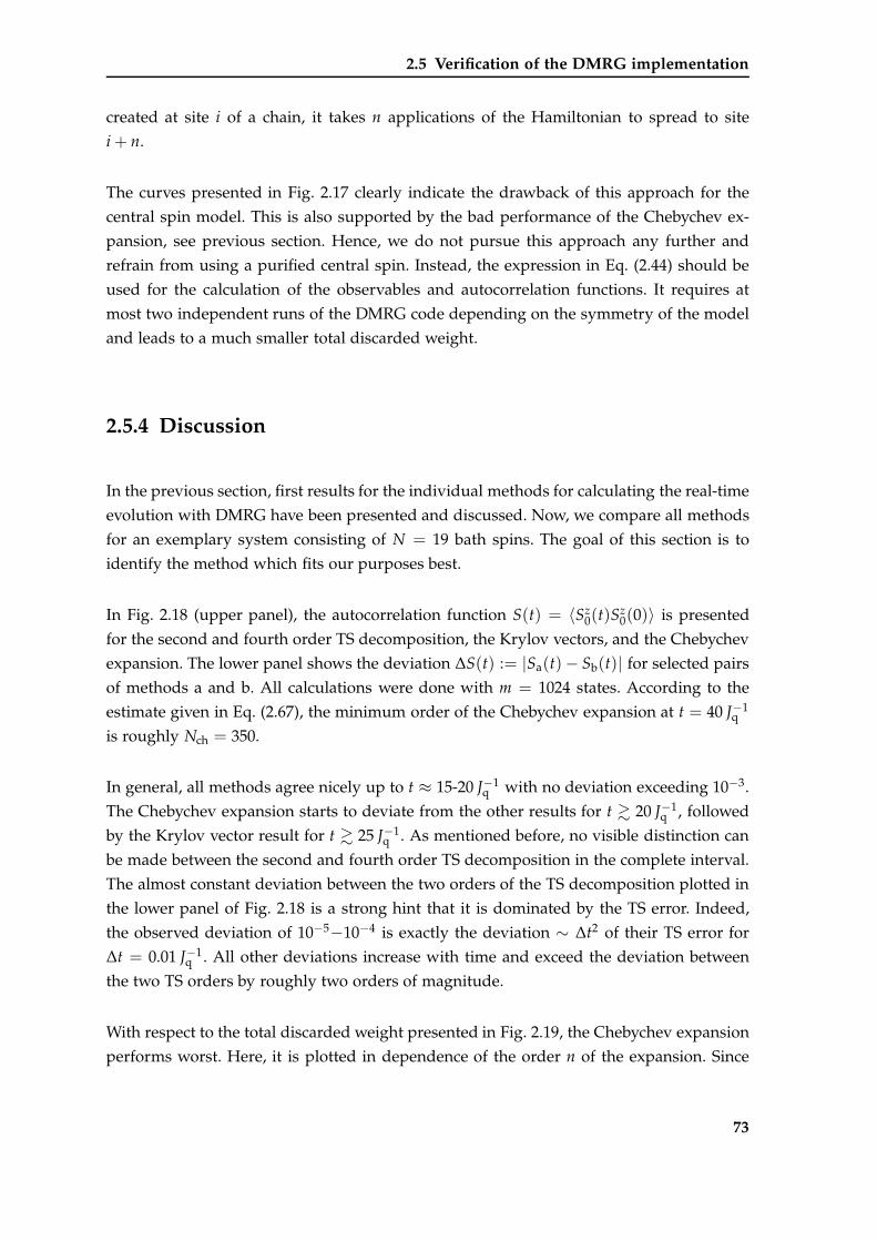
2.5 Verification of the DMRG implementation
created at site i of a chain, it takes n applications of the Hamiltonian to spread to site
i + n.
The curves presented in Fig. 2.17 clearly indicate the drawback of this approach for the
central spin model. This is also supported by the bad performance of the Chebychev ex-
pansion, see previous section. Hence, we do not pursue this approach any further and
refrain from using a purified central spin. Instead, the expression in Eq. (2.44) should be
used for the calculation of the observables and autocorrelation functions. It requires at
most two independent runs of the DMRG code depending on the symmetry of the model
and leads to a much smaller total discarded weight.
2.5.4 Discussion
In the previous section, first results for the individual methods for calculating the real-time
evolution with DMRG have been presented and discussed. Now, we compare all methods
for an exemplary system consisting of N = 19 bath spins. The goal of this section is to
identify the method which fits our purposes best.
In Fig. 2.18 (upper panel), the autocorrelation function S(t) = 〈Sz0(t)S
z0(0)〉 is presented
for the second and fourth order TS decomposition, the Krylov vectors, and the Chebychev
expansion. The lower panel shows the deviation ∆S(t) := |Sa(t)− Sb(t)| for selected pairs
of methods a and b. All calculations were done with m = 1024 states. According to the
estimate given in Eq. (2.67), the minimum order of the Chebychev expansion at t = 40 J−1q
is roughly Nch = 350.
In general, all methods agree nicely up to t ≈ 15-20 J−1q with no deviation exceeding 10−3.
The Chebychev expansion starts to deviate from the other results for t & 20 J−1q , followed
by the Krylov vector result for t & 25 J−1q . As mentioned before, no visible distinction can
be made between the second and fourth order TS decomposition in the complete interval.
The almost constant deviation between the two orders of the TS decomposition plotted in
the lower panel of Fig. 2.18 is a strong hint that it is dominated by the TS error. Indeed,
the observed deviation of 10−5−10−4 is exactly the deviation ∼ ∆t2 of their TS error for
∆t = 0.01 J−1q . All other deviations increase with time and exceed the deviation between
the two TS orders by roughly two orders of magnitude.
With respect to the total discarded weight presented in Fig. 2.19, the Chebychev expansion
performs worst. Here, it is plotted in dependence of the order n of the expansion. Since
73
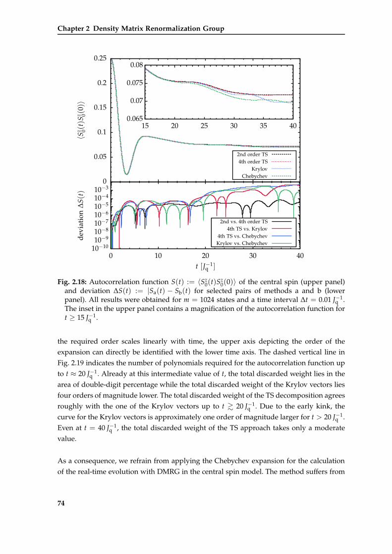
Chapter 2 Density Matrix Renormalization Group
0
0.05
0.1
0.15
0.2
0.25
〈Sz 0(
t)S
z 0(0)〉
0.065
0.07
0.075
0.08
15 20 25 30 35 40
10−1010−910−810−710−610−510−410−3
0 10 20 30 40
dev
iati
on∆
S(t)
t [J−1q ]
2nd order TS4th order TS
KrylovChebychev
2nd vs. 4th order TS4th TS vs. Krylov
4th TS vs. ChebychevKrylov vs. Chebychev
Fig. 2.18: Autocorrelation function S(t) := 〈Sz0(t)S
z0(0)〉 of the central spin (upper panel)
and deviation ∆S(t) := |Sa(t) − Sb(t) for selected pairs of methods a and b (lowerpanel). All results were obtained for m = 1024 states and a time interval ∆t = 0.01 J−1
q .The inset in the upper panel contains a magnification of the autocorrelation function fort ≥ 15 J−1
q .
the required order scales linearly with time, the upper axis depicting the order of the
expansion can directly be identified with the lower time axis. The dashed vertical line in
Fig. 2.19 indicates the number of polynomials required for the autocorrelation function up
to t ≈ 20 J−1q . Already at this intermediate value of t, the total discarded weight lies in the
area of double-digit percentage while the total discarded weight of the Krylov vectors lies
four orders of magnitude lower. The total discarded weight of the TS decomposition agrees
roughly with the one of the Krylov vectors up to t & 20 J−1q . Due to the early kink, the
curve for the Krylov vectors is approximately one order of magnitude larger for t > 20 J−1q .
Even at t = 40 J−1q , the total discarded weight of the TS approach takes only a moderate
value.
As a consequence, we refrain from applying the Chebychev expansion for the calculation
of the real-time evolution with DMRG in the central spin model. The method suffers from
74
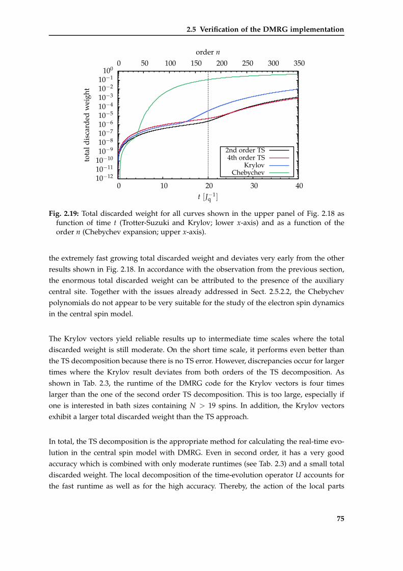
2.5 Verification of the DMRG implementation
10−1210−1110−1010−910−810−710−610−510−410−310−210−1
100
0 10 20 30 40
0 50 100 150 200 250 300 350
tota
ldis
card
edw
eigh
t
t [J−1q ]
order n
2nd order TS4th order TS
KrylovChebychev
Fig. 2.19: Total discarded weight for all curves shown in the upper panel of Fig. 2.18 asfunction of time t (Trotter-Suzuki and Krylov; lower x-axis) and as a function of theorder n (Chebychev expansion; upper x-axis).
the extremely fast growing total discarded weight and deviates very early from the other
results shown in Fig. 2.18. In accordance with the observation from the previous section,
the enormous total discarded weight can be attributed to the presence of the auxiliary
central site. Together with the issues already addressed in Sect. 2.5.2.2, the Chebychev
polynomials do not appear to be very suitable for the study of the electron spin dynamics
in the central spin model.
The Krylov vectors yield reliable results up to intermediate time scales where the total
discarded weight is still moderate. On the short time scale, it performs even better than
the TS decomposition because there is no TS error. However, discrepancies occur for larger
times where the Krylov result deviates from both orders of the TS decomposition. As
shown in Tab. 2.3, the runtime of the DMRG code for the Krylov vectors is four times
larger than the one of the second order TS decomposition. This is too large, especially if
one is interested in bath sizes containing N > 19 spins. In addition, the Krylov vectors
exhibit a larger total discarded weight than the TS approach.
In total, the TS decomposition is the appropriate method for calculating the real-time evo-
lution in the central spin model with DMRG. Even in second order, it has a very good
accuracy which is combined with only moderate runtimes (see Tab. 2.3) and a small total
discarded weight. The local decomposition of the time-evolution operator U accounts for
the fast runtime as well as for the high accuracy. Thereby, the action of the local parts
75
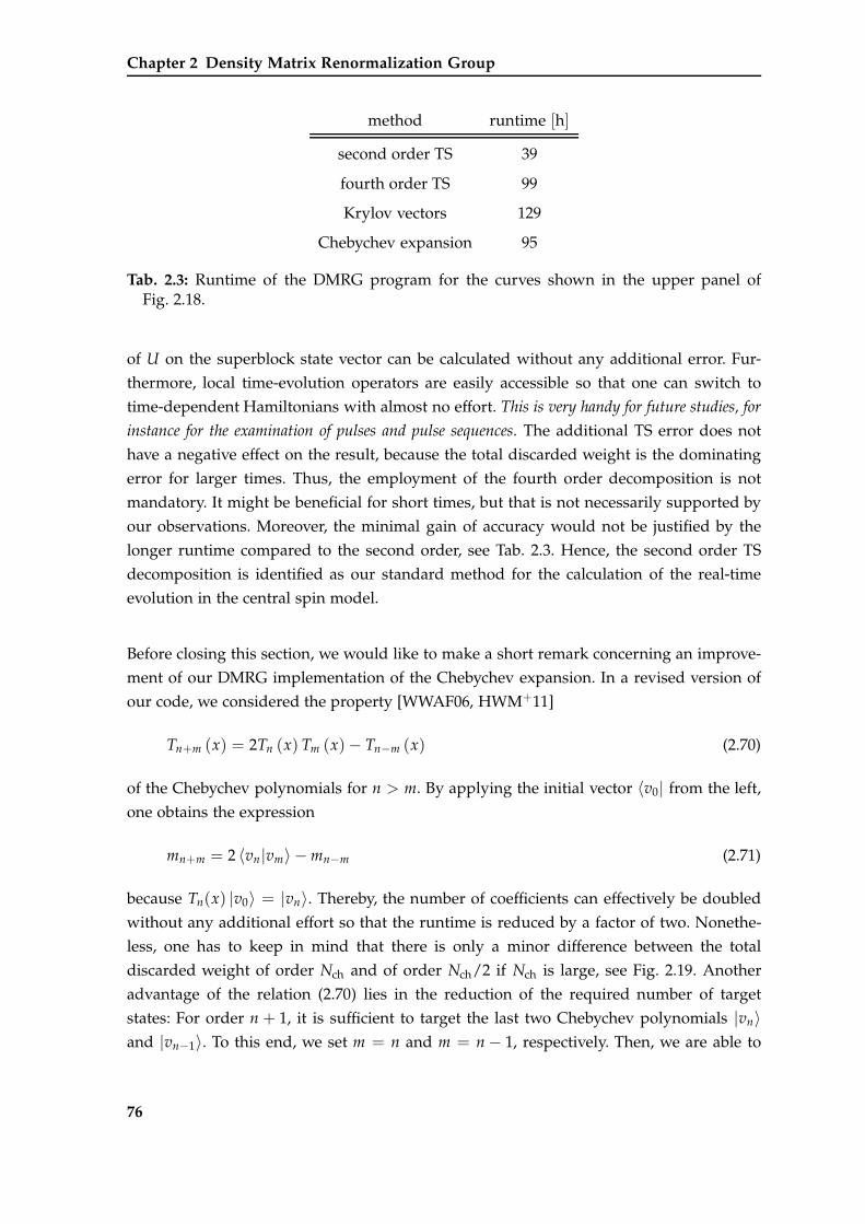
Chapter 2 Density Matrix Renormalization Group
method runtime [h]
second order TS 39
fourth order TS 99
Krylov vectors 129
Chebychev expansion 95
Tab. 2.3: Runtime of the DMRG program for the curves shown in the upper panel ofFig. 2.18.
of U on the superblock state vector can be calculated without any additional error. Fur-
thermore, local time-evolution operators are easily accessible so that one can switch to
time-dependent Hamiltonians with almost no effort. This is very handy for future studies, for
instance for the examination of pulses and pulse sequences. The additional TS error does not
have a negative effect on the result, because the total discarded weight is the dominating
error for larger times. Thus, the employment of the fourth order decomposition is not
mandatory. It might be beneficial for short times, but that is not necessarily supported by
our observations. Moreover, the minimal gain of accuracy would not be justified by the
longer runtime compared to the second order, see Tab. 2.3. Hence, the second order TS
decomposition is identified as our standard method for the calculation of the real-time
evolution in the central spin model.
Before closing this section, we would like to make a short remark concerning an improve-
ment of our DMRG implementation of the Chebychev expansion. In a revised version of
our code, we considered the property [WWAF06, HWM+11]
Tn+m (x) = 2Tn (x) Tm (x)− Tn−m (x) (2.70)
of the Chebychev polynomials for n > m. By applying the initial vector 〈v0| from the left,
one obtains the expression
mn+m = 2 〈vn|vm〉 − mn−m (2.71)
because Tn(x) |v0〉 = |vn〉. Thereby, the number of coefficients can effectively be doubled
without any additional effort so that the runtime is reduced by a factor of two. Nonethe-
less, one has to keep in mind that there is only a minor difference between the total
discarded weight of order Nch and of order Nch/2 if Nch is large, see Fig. 2.19. Another
advantage of the relation (2.70) lies in the reduction of the required number of target
states: For order n + 1, it is sufficient to target the last two Chebychev polynomials |vn〉and |vn−1〉. To this end, we set m = n and m = n − 1, respectively. Then, we are able to
76
2.6 Errors & limits
calculate the odd orders by the relation
m2n+1 = 2 〈vn|vn−1〉 − m1 (2.72a)
and the even orders by the relation
m2n = 2 〈vn|vn〉 − m0. (2.72b)
One might suppose that this procedure may lead to a reduction of the total discarded
weight because the targeting of the initial state |v0〉 is not required anymore. However,
this was not observed indicating that the enormous growth of the total discarded weight
has to be attributed to the presence of the purified central spin and not to the permanent
targeting of the initial state |v0〉.
2.6 Errors & limits
In the following, we discuss the errors and the limits of the real-time evolution with the sec-
ond order TS decomposition on the basis of the central spin model in the zero-field limit.
Furthermore, the scaling of the errors and the performance of the algorithm in depen-
dence of the number of bath spins are addressed. As before, the focus lies on intermediate
time scales t ≥ 20 J−1q . This time scale is particularly important for the plateau emerging
at t & 5 J−1q which is discussed in more detail later on. Due to the absence of an external
field, the central spin model in the zero-field limit corresponds to the most complex case
because spin-flips between bath and central spin are not suppressed. In the presence of
an external field, the investigation of the model is simplified because the field polarizes
the spins. This leads to a simplification of the structure of the superblock state, implying
faster runtimes and smaller total discarded weights as less states become important, see
Sect. 2.7.2.
In the real-time evolution with DMRG based on the TS decomposition, two parameters
can be tuned: The number of tracked states m and the time interval ∆t. At first, we keep
the number of states m = 1024 fixed and examine the influence of the time interval ∆t. In
Fig. 2.20, the magnetization of the central spin is presented for N = 19 (upper panel) and
N = 49 (lower panel) bath spins for the time intervals ∆t = 0.01 J−1q , ∆t = 0.02 J−1
q and
∆t = 0.05 J−1q . All curves for N = 19 bath spins are in good agreement. The magnification
shown in the inset of the upper panel reveals some small discrepancies close to t = 40 J−1q .
But the relative deviation between the curves for the different values of ∆t is still less than
10−3. For N = 49 bath spins, the deviation increases to the order of roughly 10−2. In total,
the agreement between all curves is still excellent in the complete time interval.
77
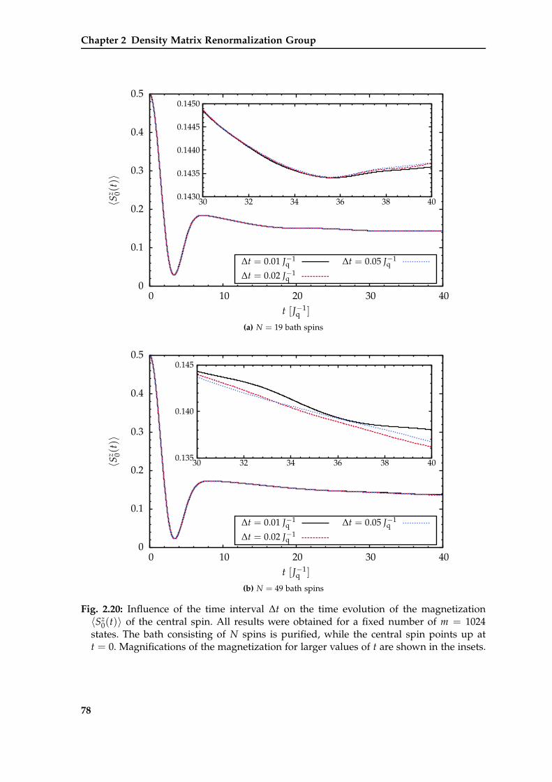
Chapter 2 Density Matrix Renormalization Group
0
0.1
0.2
0.3
0.4
0.5
0 10 20 30 40
〈Sz 0(
t)〉
t [J−1q ]
0.1430
0.1435
0.1440
0.1445
0.1450
30 32 34 36 38 40
∆t = 0.01 J−1q
∆t = 0.02 J−1q
∆t = 0.05 J−1q
(a) N = 19 bath spins
0
0.1
0.2
0.3
0.4
0.5
0 10 20 30 40
〈Sz 0(
t)〉
t [J−1q ]
0.135
0.140
0.145
30 32 34 36 38 40
∆t = 0.01 J−1q
∆t = 0.02 J−1q
∆t = 0.05 J−1q
(b) N = 49 bath spins
Fig. 2.20: Influence of the time interval ∆t on the time evolution of the magnetization〈Sz
0(t)〉 of the central spin. All results were obtained for a fixed number of m = 1024states. The bath consisting of N spins is purified, while the central spin points up att = 0. Magnifications of the magnetization for larger values of t are shown in the insets.
78
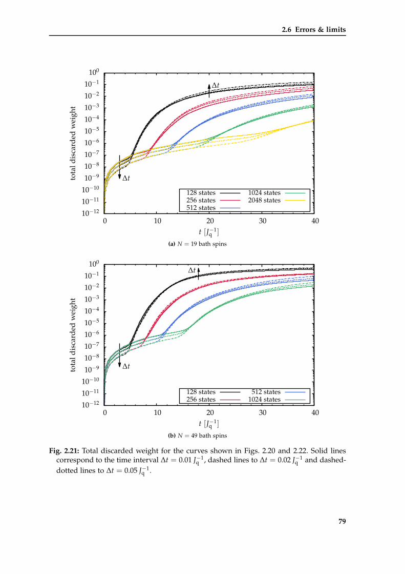
2.6 Errors & limits
10−12
10−11
10−10
10−9
10−8
10−7
10−6
10−5
10−4
10−3
10−2
10−1
100
0 10 20 30 40
tota
ldis
card
edw
eigh
t
t [J−1q ]
∆t
∆t
128 states256 states512 states
1024 states2048 states
(a) N = 19 bath spins
10−12
10−11
10−10
10−9
10−8
10−7
10−6
10−5
10−4
10−3
10−2
10−1
100
0 10 20 30 40
tota
ldis
card
edw
eigh
t
t [J−1q ]
∆t
∆t
128 states256 states
512 states1024 states
(b) N = 49 bath spins
Fig. 2.21: Total discarded weight for the curves shown in Figs. 2.20 and 2.22. Solid linescorrespond to the time interval ∆t = 0.01 J−1
q , dashed lines to ∆t = 0.02 J−1q and dashed-
dotted lines to ∆t = 0.05 J−1q .
79
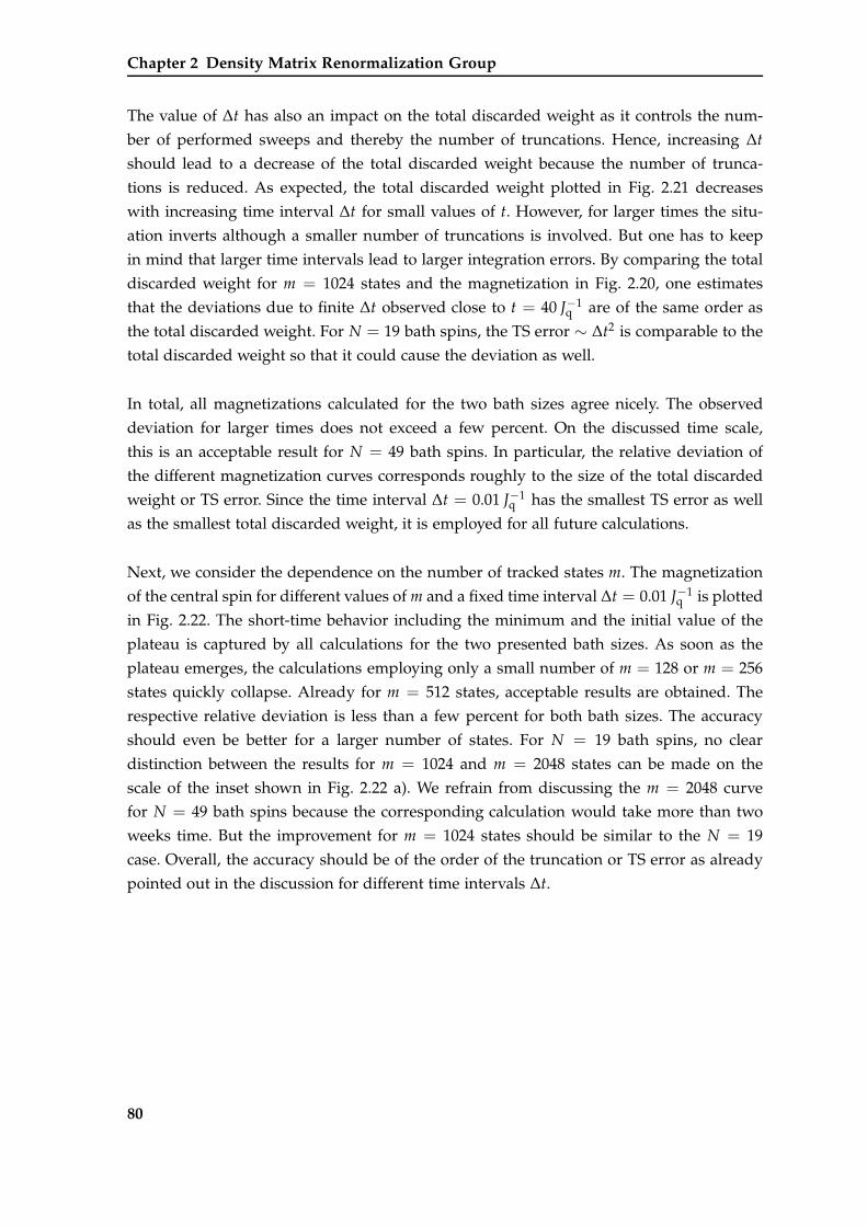
Chapter 2 Density Matrix Renormalization Group
The value of ∆t has also an impact on the total discarded weight as it controls the num-
ber of performed sweeps and thereby the number of truncations. Hence, increasing ∆t
should lead to a decrease of the total discarded weight because the number of trunca-
tions is reduced. As expected, the total discarded weight plotted in Fig. 2.21 decreases
with increasing time interval ∆t for small values of t. However, for larger times the situ-
ation inverts although a smaller number of truncations is involved. But one has to keep
in mind that larger time intervals lead to larger integration errors. By comparing the total
discarded weight for m = 1024 states and the magnetization in Fig. 2.20, one estimates
that the deviations due to finite ∆t observed close to t = 40 J−1q are of the same order as
the total discarded weight. For N = 19 bath spins, the TS error ∼ ∆t2 is comparable to the
total discarded weight so that it could cause the deviation as well.
In total, all magnetizations calculated for the two bath sizes agree nicely. The observed
deviation for larger times does not exceed a few percent. On the discussed time scale,
this is an acceptable result for N = 49 bath spins. In particular, the relative deviation of
the different magnetization curves corresponds roughly to the size of the total discarded
weight or TS error. Since the time interval ∆t = 0.01 J−1q has the smallest TS error as well
as the smallest total discarded weight, it is employed for all future calculations.
Next, we consider the dependence on the number of tracked states m. The magnetization
of the central spin for different values of m and a fixed time interval ∆t = 0.01 J−1q is plotted
in Fig. 2.22. The short-time behavior including the minimum and the initial value of the
plateau is captured by all calculations for the two presented bath sizes. As soon as the
plateau emerges, the calculations employing only a small number of m = 128 or m = 256
states quickly collapse. Already for m = 512 states, acceptable results are obtained. The
respective relative deviation is less than a few percent for both bath sizes. The accuracy
should even be better for a larger number of states. For N = 19 bath spins, no clear
distinction between the results for m = 1024 and m = 2048 states can be made on the
scale of the inset shown in Fig. 2.22 a). We refrain from discussing the m = 2048 curve
for N = 49 bath spins because the corresponding calculation would take more than two
weeks time. But the improvement for m = 1024 states should be similar to the N = 19
case. Overall, the accuracy should be of the order of the truncation or TS error as already
pointed out in the discussion for different time intervals ∆t.
80
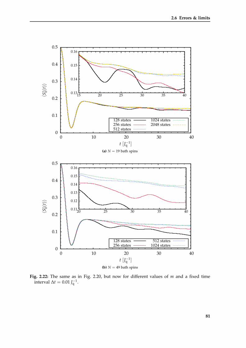
2.6 Errors & limits
0
0.1
0.2
0.3
0.4
0.5
0 10 20 30 40
〈Sz 0(
t)〉
t [J−1q ]
0.13
0.14
0.15
0.16
15 20 25 30 35 40
128 states256 states512 states
1024 states2048 states
(a) N = 19 bath spins
0
0.1
0.2
0.3
0.4
0.5
0 10 20 30 40
〈Sz 0(
t)〉
t [J−1q ]
0.11
0.12
0.13
0.14
0.15
0.16
20 25 30 35 40
128 states256 states
512 states1024 states
(b) N = 49 bath spins
Fig. 2.22: The same as in Fig. 2.20, but now for different values of m and a fixed timeinterval ∆t = 0.01 J−1
q .
81
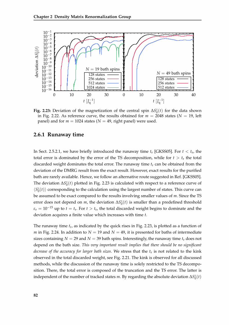
Chapter 2 Density Matrix Renormalization Group
10−1610−1510−1410−1310−1210−1110−1010−910−810−710−610−510−410−310−210−1
0 10 20 30
dev
iati
on∆
Sz 0(
t)
t [J−1q ]
N = 19 bath spins
0 10 20 30 40t [J−1
q ]
N = 49 bath spins128 states256 states512 states
1024 states
128 states256 states512 states
Fig. 2.23: Deviation of the magnetization of the central spin ∆Sz0(t) for the data shown
in Fig. 2.22. As reference curve, the results obtained for m = 2048 states (N = 19, leftpanel) and for m = 1024 states (N = 49, right panel) were used.
2.6.1 Runaway time
In Sect. 2.5.2.1, we have briefly introduced the runaway time tr [GKSS05]. For t < tr, the
total error is dominated by the error of the TS decomposition, while for t > tr the total
discarded weight dominates the total error. The runaway time tr can be obtained from the
deviation of the DMRG result from the exact result. However, exact results for the purified
bath are rarely available. Hence, we follow an alternative route suggested in Ref. [GKSS05].
The deviation ∆Sz0(t) plotted in Fig. 2.23 is calculated with respect to a reference curve of
〈Sz0(t)〉 corresponding to the calculation using the largest number of states. This curve can
be assumed to be exact compared to the results involving smaller values of m. Since the TS
error does not depend on m, the deviation ∆Sz0(t) is smaller than a predefined threshold
εr = 10−15 up to t = tr. For t > tr, the total discarded weight begins to dominate and the
deviation acquires a finite value which increases with time t.
The runaway time tr, as indicated by the quick rises in Fig. 2.23, is plotted as a function of
m in Fig. 2.24. In addition to N = 19 and N = 49, it is presented for baths of intermediate
sizes containing N = 29 and N = 39 bath spins. Interestingly, the runaway time tr does not
depend on the bath size. This very important result implies that there should be no significant
decrease of the accuracy for larger bath sizes. We stress that the tr is not related to the kink
observed in the total discarded weight, see Fig. 2.21. The kink is observed for all discussed
methods, while the discussion of the runaway time is solely restricted to the TS decompo-
sition. There, the total error is composed of the truncation and the TS error. The latter is
independent of the number of tracked states m. By regarding the absolute deviation ∆Sz0(t)
82
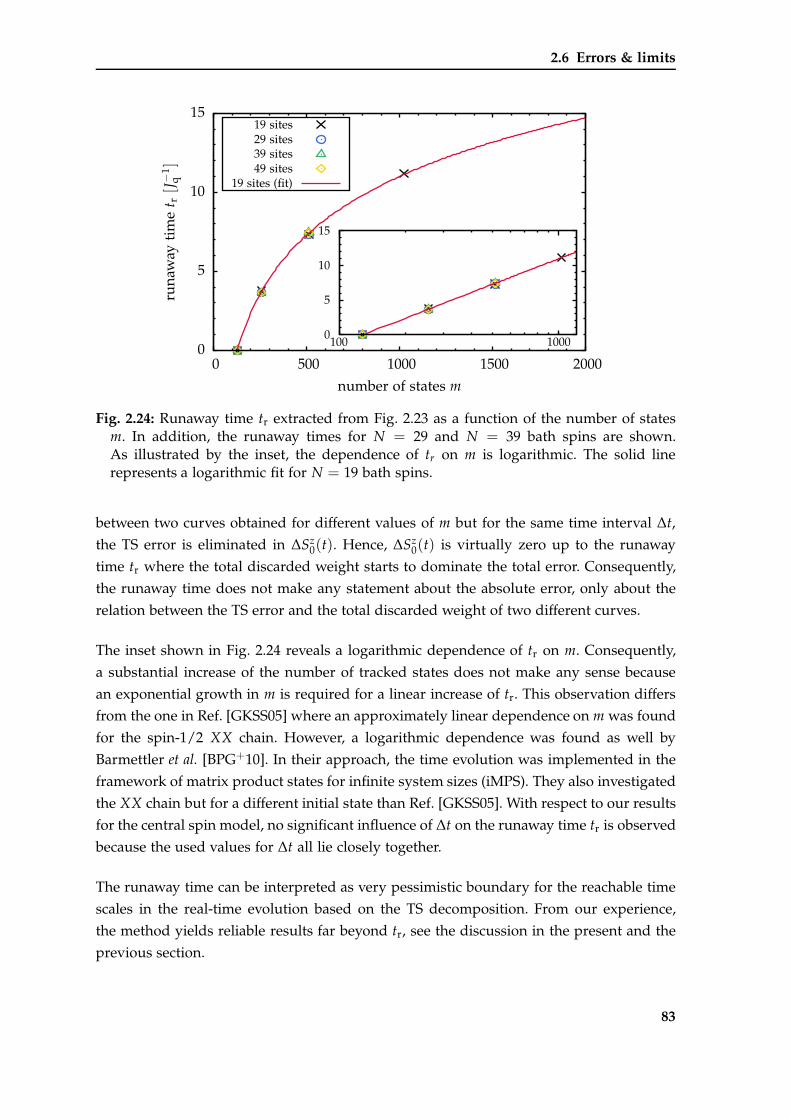
2.6 Errors & limits
0
5
10
15
0 500 1000 1500 2000
runa
way
tim
et r[J−
1q
]
number of states m
0
5
10
15
100 1000
19 sites29 sites39 sites49 sites
19 sites (fit)
Fig. 2.24: Runaway time tr extracted from Fig. 2.23 as a function of the number of statesm. In addition, the runaway times for N = 29 and N = 39 bath spins are shown.As illustrated by the inset, the dependence of tr on m is logarithmic. The solid linerepresents a logarithmic fit for N = 19 bath spins.
between two curves obtained for different values of m but for the same time interval ∆t,
the TS error is eliminated in ∆Sz0(t). Hence, ∆Sz
0(t) is virtually zero up to the runaway
time tr where the total discarded weight starts to dominate the total error. Consequently,
the runaway time does not make any statement about the absolute error, only about the
relation between the TS error and the total discarded weight of two different curves.
The inset shown in Fig. 2.24 reveals a logarithmic dependence of tr on m. Consequently,
a substantial increase of the number of tracked states does not make any sense because
an exponential growth in m is required for a linear increase of tr. This observation differs
from the one in Ref. [GKSS05] where an approximately linear dependence on m was found
for the spin-1/2 XX chain. However, a logarithmic dependence was found as well by
Barmettler et al. [BPG+10]. In their approach, the time evolution was implemented in the
framework of matrix product states for infinite system sizes (iMPS). They also investigated
the XX chain but for a different initial state than Ref. [GKSS05]. With respect to our results
for the central spin model, no significant influence of ∆t on the runaway time tr is observed
because the used values for ∆t all lie closely together.
The runaway time can be interpreted as very pessimistic boundary for the reachable time
scales in the real-time evolution based on the TS decomposition. From our experience,
the method yields reliable results far beyond tr, see the discussion in the present and the
previous section.
83
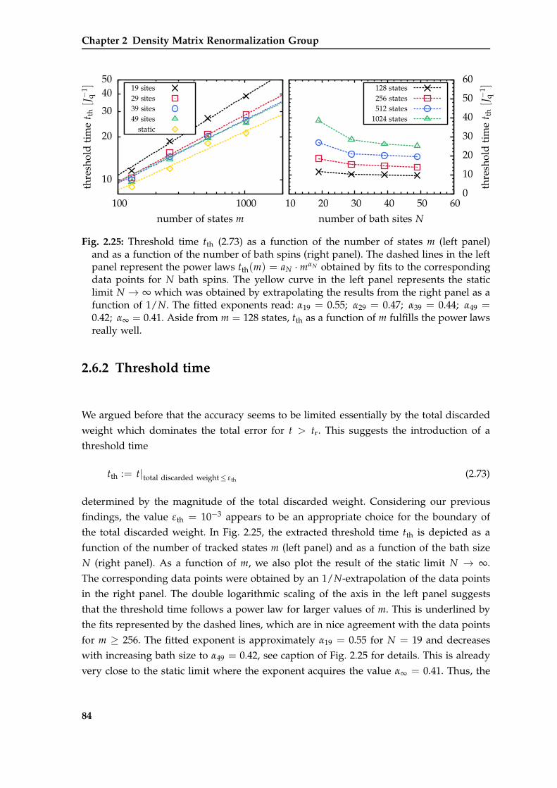
Chapter 2 Density Matrix Renormalization Group
10
20
30
4050
100 1000
thre
shol
dti
me
t th[J−
1q
]
number of states m
10 20 30 40 50 600
10
20
30
40
50
60
thre
shol
dti
me
t th[J−
1q
]
number of bath sites N
19 sites29 sites39 sites49 sites
static
128 states256 states512 states
1024 states
Fig. 2.25: Threshold time tth (2.73) as a function of the number of states m (left panel)and as a function of the number of bath spins (right panel). The dashed lines in the leftpanel represent the power laws tth(m) = aN · mαN obtained by fits to the correspondingdata points for N bath spins. The yellow curve in the left panel represents the staticlimit N → ∞ which was obtained by extrapolating the results from the right panel as afunction of 1/N. The fitted exponents read: α19 = 0.55; α29 = 0.47; α39 = 0.44; α49 =0.42; α∞ = 0.41. Aside from m = 128 states, tth as a function of m fulfills the power lawsreally well.
2.6.2 Threshold time
We argued before that the accuracy seems to be limited essentially by the total discarded
weight which dominates the total error for t > tr. This suggests the introduction of a
threshold time
tth := t|total discarded weight≤ εth(2.73)
determined by the magnitude of the total discarded weight. Considering our previous
findings, the value εth = 10−3 appears to be an appropriate choice for the boundary of
the total discarded weight. In Fig. 2.25, the extracted threshold time tth is depicted as a
function of the number of tracked states m (left panel) and as a function of the bath size
N (right panel). As a function of m, we also plot the result of the static limit N → ∞.
The corresponding data points were obtained by an 1/N-extrapolation of the data points
in the right panel. The double logarithmic scaling of the axis in the left panel suggests
that the threshold time follows a power law for larger values of m. This is underlined by
the fits represented by the dashed lines, which are in nice agreement with the data points
for m ≥ 256. The fitted exponent is approximately α19 = 0.55 for N = 19 and decreases
with increasing bath size to α49 = 0.42, see caption of Fig. 2.25 for details. This is already
very close to the static limit where the exponent acquires the value α∞ = 0.41. Thus, the
84
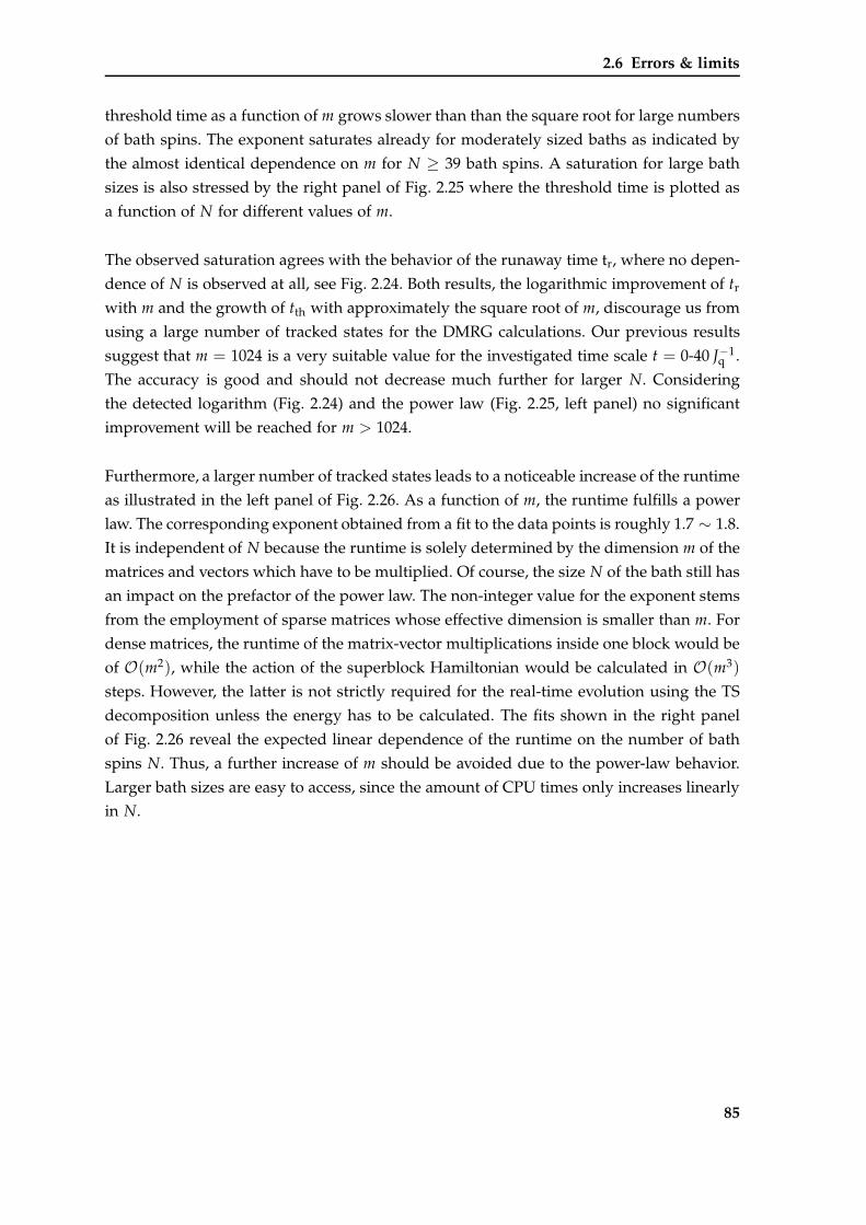
2.6 Errors & limits
threshold time as a function of m grows slower than than the square root for large numbers
of bath spins. The exponent saturates already for moderately sized baths as indicated by
the almost identical dependence on m for N ≥ 39 bath spins. A saturation for large bath
sizes is also stressed by the right panel of Fig. 2.25 where the threshold time is plotted as
a function of N for different values of m.
The observed saturation agrees with the behavior of the runaway time tr, where no depen-
dence of N is observed at all, see Fig. 2.24. Both results, the logarithmic improvement of tr
with m and the growth of tth with approximately the square root of m, discourage us from
using a large number of tracked states for the DMRG calculations. Our previous results
suggest that m = 1024 is a very suitable value for the investigated time scale t = 0-40 J−1q .
The accuracy is good and should not decrease much further for larger N. Considering
the detected logarithm (Fig. 2.24) and the power law (Fig. 2.25, left panel) no significant
improvement will be reached for m > 1024.
Furthermore, a larger number of tracked states leads to a noticeable increase of the runtime
as illustrated in the left panel of Fig. 2.26. As a function of m, the runtime fulfills a power
law. The corresponding exponent obtained from a fit to the data points is roughly 1.7 ∼ 1.8.
It is independent of N because the runtime is solely determined by the dimension m of the
matrices and vectors which have to be multiplied. Of course, the size N of the bath still has
an impact on the prefactor of the power law. The non-integer value for the exponent stems
from the employment of sparse matrices whose effective dimension is smaller than m. For
dense matrices, the runtime of the matrix-vector multiplications inside one block would be
of O(m2), while the action of the superblock Hamiltonian would be calculated in O(m3)
steps. However, the latter is not strictly required for the real-time evolution using the TS
decomposition unless the energy has to be calculated. The fits shown in the right panel
of Fig. 2.26 reveal the expected linear dependence of the runtime on the number of bath
spins N. Thus, a further increase of m should be avoided due to the power-law behavior.
Larger bath sizes are easy to access, since the amount of CPU times only increases linearly
in N.
85
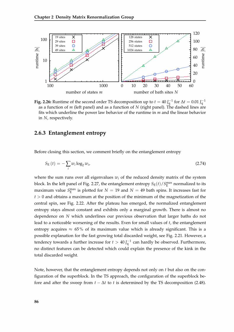
Chapter 2 Density Matrix Renormalization Group
1
10
100
100 1000
runt
ime[h]
number of states m
0 10 20 30 40 50 600
20
40
60
80
100
120
runt
ime[h]
number of bath sites N
19 sites29 sites39 sites49 sites
128 states256 states512 states
1024 states
Fig. 2.26: Runtime of the second order TS decomposition up to t = 40 J−1q for ∆t = 0.01 J−1
qas a function of m (left panel) and as a function of N (right panel). The dashed lines arefits which underline the power law behavior of the runtime in m and the linear behaviorin N, respectively.
2.6.3 Entanglement entropy
Before closing this section, we comment briefly on the entanglement entropy
SE (t) = −∑i
wi log2 wi, (2.74)
where the sum runs over all eigenvalues wi of the reduced density matrix of the system
block. In the left panel of Fig. 2.27, the entanglement entropy SE(t)/SmaxE normalized to its
maximum value SmaxE is plotted for N = 19 and N = 49 bath spins. It increases fast for
t > 0 and obtains a maximum at the position of the minimum of the magnetization of the
central spin, see Fig. 2.22. After the plateau has emerged, the normalized entanglement
entropy stays almost constant and exhibits only a marginal growth. There is almost no
dependence on N which underlines our previous observation that larger baths do not
lead to a noticeable worsening of the results. Even for small values of t, the entanglement
entropy acquires ≈ 65 % of its maximum value which is already significant. This is a
possible explanation for the fast growing total discarded weight, see Fig. 2.21. However, a
tendency towards a further increase for t > 40 J−1q can hardly be observed. Furthermore,
no distinct features can be detected which could explain the presence of the kink in the
total discarded weight.
Note, however, that the entanglement entropy depends not only on t but also on the con-
figuration of the superblock. In the TS approach, the configuration of the superblock be-
fore and after the sweep from t − ∆t to t is determined by the TS decomposition (2.48).
86
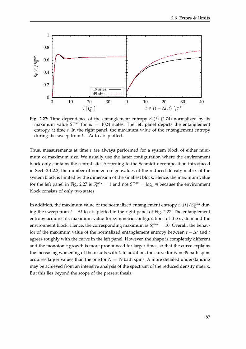
2.6 Errors & limits
0
0.2
0.4
0.6
0.8
1
0 10 20 30
SE(t)/
Sm
axE
t [J−1q ]
0 10 20 30 40t ∈ (t − ∆t, t) [J−1
q ]
19 sites49 sites
Fig. 2.27: Time dependence of the entanglement entropy Se(t) (2.74) normalized by itsmaximum value Smax
E for m = 1024 states. The left panel depicts the entanglemententropy at time t. In the right panel, the maximum value of the entanglement entropyduring the sweep from t − ∆t to t is plotted.
Thus, measurements at time t are always performed for a system block of either mini-
mum or maximum size. We usually use the latter configuration where the environment
block only contains the central site. According to the Schmidt decomposition introduced
in Sect. 2.1.2.3, the number of non-zero eigenvalues of the reduced density matrix of the
system block is limited by the dimension of the smallest block. Hence, the maximum value
for the left panel in Fig. 2.27 is SmaxE = 1 and not Smax
E = log2 m because the environment
block consists of only two states.
In addition, the maximum value of the normalized entanglement entropy SE(t)/SmaxE dur-
ing the sweep from t − ∆t to t is plotted in the right panel of Fig. 2.27. The entanglement
entropy acquires its maximum value for symmetric configurations of the system and the
environment block. Hence, the corresponding maximum is SmaxE = 10. Overall, the behav-
ior of the maximum value of the normalized entanglement entropy between t − ∆t and t
agrees roughly with the curve in the left panel. However, the shape is completely different
and the monotonic growth is more pronounced for larger times so that the curve explains
the increasing worsening of the results with t. In addition, the curve for N = 49 bath spins
acquires larger values than the one for N = 19 bath spins. A more detailed understanding
may be achieved from an intensive analysis of the spectrum of the reduced density matrix.
But this lies beyond the scope of the present thesis.
87
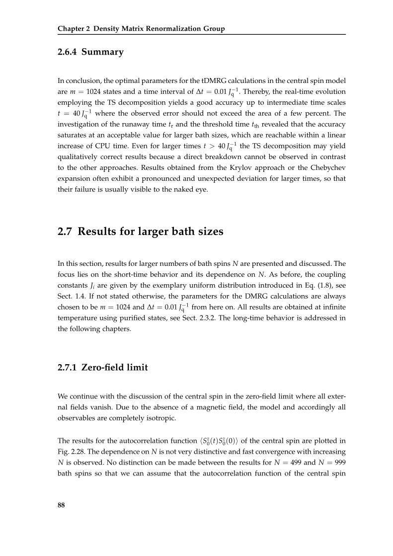
Chapter 2 Density Matrix Renormalization Group
2.6.4 Summary
In conclusion, the optimal parameters for the tDMRG calculations in the central spin model
are m = 1024 states and a time interval of ∆t = 0.01 J−1q . Thereby, the real-time evolution
employing the TS decomposition yields a good accuracy up to intermediate time scales
t = 40 J−1q where the observed error should not exceed the area of a few percent. The
investigation of the runaway time tr and the threshold time tth revealed that the accuracy
saturates at an acceptable value for larger bath sizes, which are reachable within a linear
increase of CPU time. Even for larger times t > 40 J−1q the TS decomposition may yield
qualitatively correct results because a direct breakdown cannot be observed in contrast
to the other approaches. Results obtained from the Krylov approach or the Chebychev
expansion often exhibit a pronounced and unexpected deviation for larger times, so that
their failure is usually visible to the naked eye.
2.7 Results for larger bath sizes
In this section, results for larger numbers of bath spins N are presented and discussed. The
focus lies on the short-time behavior and its dependence on N. As before, the coupling
constants Ji are given by the exemplary uniform distribution introduced in Eq. (1.8), see
Sect. 1.4. If not stated otherwise, the parameters for the DMRG calculations are always
chosen to be m = 1024 and ∆t = 0.01 J−1q from here on. All results are obtained at infinite
temperature using purified states, see Sect. 2.3.2. The long-time behavior is addressed in
the following chapters.
2.7.1 Zero-field limit
We continue with the discussion of the central spin in the zero-field limit where all exter-
nal fields vanish. Due to the absence of a magnetic field, the model and accordingly all
observables are completely isotropic.
The results for the autocorrelation function 〈Sz0(t)S
z0(0)〉 of the central spin are plotted in
Fig. 2.28. The dependence on N is not very distinctive and fast convergence with increasing
N is observed. No distinction can be made between the results for N = 499 and N = 999
bath spins so that we can assume that the autocorrelation function of the central spin
88
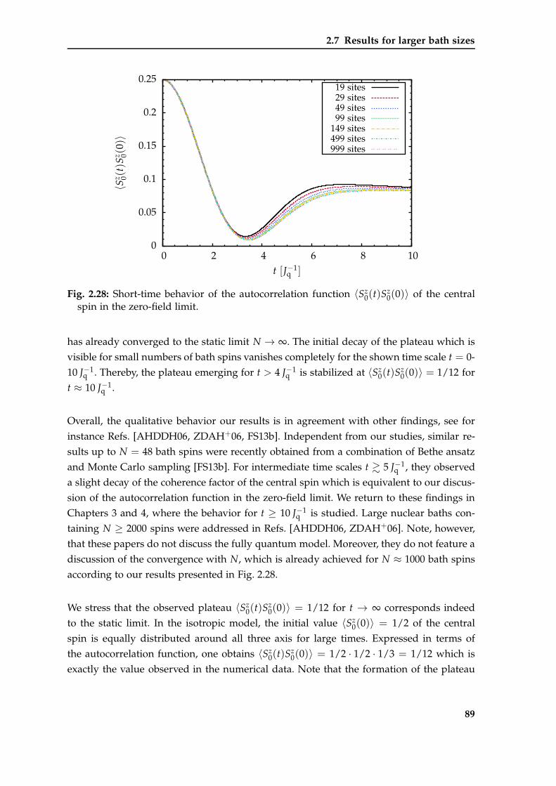
2.7 Results for larger bath sizes
0
0.05
0.1
0.15
0.2
0.25
0 2 4 6 8 10
〈Sz 0(
t)S
z 0(0)〉
t [J−1q ]
19 sites29 sites49 sites99 sites
149 sites499 sites999 sites
Fig. 2.28: Short-time behavior of the autocorrelation function 〈Sz0(t)S
z0(0)〉 of the central
spin in the zero-field limit.
has already converged to the static limit N → ∞. The initial decay of the plateau which is
visible for small numbers of bath spins vanishes completely for the shown time scale t = 0-
10 J−1q . Thereby, the plateau emerging for t > 4 J−1
q is stabilized at 〈Sz0(t)S
z0(0)〉 = 1/12 for
t ≈ 10 J−1q .
Overall, the qualitative behavior our results is in agreement with other findings, see for
instance Refs. [AHDDH06, ZDAH+06, FS13b]. Independent from our studies, similar re-
sults up to N = 48 bath spins were recently obtained from a combination of Bethe ansatz
and Monte Carlo sampling [FS13b]. For intermediate time scales t & 5 J−1q , they observed
a slight decay of the coherence factor of the central spin which is equivalent to our discus-
sion of the autocorrelation function in the zero-field limit. We return to these findings in
Chapters 3 and 4, where the behavior for t ≥ 10 J−1q is studied. Large nuclear baths con-
taining N ≥ 2000 spins were addressed in Refs. [AHDDH06, ZDAH+06]. Note, however,
that these papers do not discuss the fully quantum model. Moreover, they do not feature a
discussion of the convergence with N, which is already achieved for N ≈ 1000 bath spins
according to our results presented in Fig. 2.28.
We stress that the observed plateau 〈Sz0(t)S
z0(0)〉 = 1/12 for t → ∞ corresponds indeed
to the static limit. In the isotropic model, the initial value 〈Sz0(0)〉 = 1/2 of the central
spin is equally distributed around all three axis for large times. Expressed in terms of
the autocorrelation function, one obtains 〈Sz0(t)S
z0(0)〉 = 1/2 · 1/2 · 1/3 = 1/12 which is
exactly the value observed in the numerical data. Note that the formation of the plateau
89
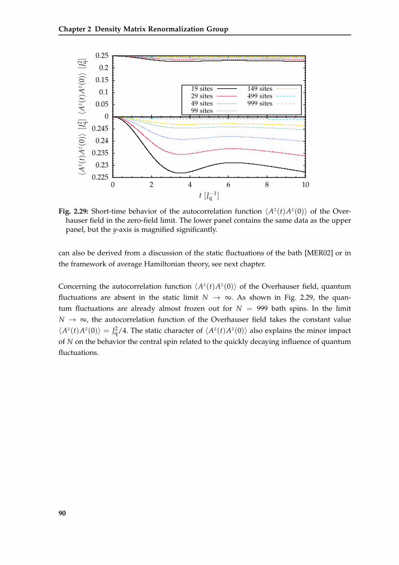
Chapter 2 Density Matrix Renormalization Group
0
0.05
0.1
0.15
0.2
0.25
〈Az(t)A
z(0)〉
[J2 q]
0.225
0.23
0.235
0.24
0.245
0 2 4 6 8 10
〈Az(t)A
z(0)〉
[J2 q]
t [J−1q ]
19 sites29 sites49 sites99 sites
149 sites499 sites999 sites
Fig. 2.29: Short-time behavior of the autocorrelation function 〈Az(t)Az(0)〉 of the Over-hauser field in the zero-field limit. The lower panel contains the same data as the upperpanel, but the y-axis is magnified significantly.
can also be derived from a discussion of the static fluctuations of the bath [MER02] or in
the framework of average Hamiltonian theory, see next chapter.
Concerning the autocorrelation function 〈Az(t)Az(0)〉 of the Overhauser field, quantum
fluctuations are absent in the static limit N → ∞. As shown in Fig. 2.29, the quan-
tum fluctuations are already almost frozen out for N = 999 bath spins. In the limit
N → ∞, the autocorrelation function of the Overhauser field takes the constant value
〈Az(t)Az(0)〉 = J2q/4. The static character of 〈Az(t)Az(0)〉 also explains the minor impact
of N on the behavior the central spin related to the quickly decaying influence of quantum
fluctuations.
90
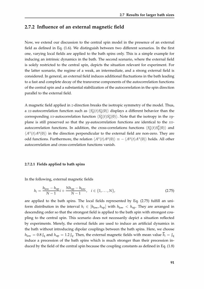
2.7 Results for larger bath sizes
2.7.2 Influence of an external magnetic field
Now, we extend our discussion to the central spin model in the presence of an external
field as defined in Eq. (1.6). We distinguish between two different scenarios. In the first
one, varying local fields are applied to the bath spins only. This is a simple example for
inducing an intrinsic dynamics in the bath. The second scenario, where the external field
is solely restricted to the central spin, depicts the situation relevant for experiment. For
the latter scenario, the regime of a weak, an intermediate, and a strong external field is
considered. In general, an external field induces additional fluctuations in the bath leading
to a fast and complete decay of the transverse components of the autocorrelation functions
of the central spin and a substantial stabilization of the autocorrelation in the spin direction
parallel to the external field.
A magnetic field applied in z-direction breaks the isotropic symmetry of the model. Thus,
a zz-autocorrelation function such as 〈Sz0(t)S
z0(0)〉 displays a different behavior than the
corresponding xx-autocorrelation function 〈Sx0(t)S
x0(0)〉. Note that the isotropy in the xy-
plane is still preserved so that the yy-autocorrelation functions are identical to the xx-
autocorrelation functions. In addition, the cross-correlations functions 〈Sx0(t)S
y0(0)〉 and
〈Ax(t)Ay(0)〉 in the direction perpendicular to the external field are non-zero. They are
odd functions. Furthermore, the relation 〈Ax(t)Ay(0)〉 ≡ − 〈Ay(t)Ax(0)〉 holds. All other
autocorrelation and cross-correlation functions vanish.
2.7.2.1 Fields applied to bath spins
In the following, external magnetic fields
hi =hlow − hup
N − 1i +
Nhup − hlow
N − 1, i ∈ 1, . . . , N, (2.75)
are applied to the bath spins. The local fields represented by Eq. (2.75) fulfill an uni-
form distribution in the interval hi ∈ [hlow, hup] with hlow < hup. They are arranged in
descending order so that the strongest field is applied to the bath spin with strongest cou-
pling to the central spin. This scenario does not necessarily depict a situation reflected
by experiments. Merely, the external fields are used to induce an artificial dynamics in
the bath without introducing dipolar couplings between the bath spins. Here, we choose
hlow = 0.8 Jq and hup = 1.2 Jq. Then, the external magnetic fields with mean value hi = Jq
induce a precession of the bath spins which is much stronger than their precession in-
duced by the field of the central spin because the coupling constants as defined in Eq. (1.8)
91
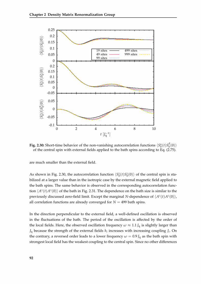
Chapter 2 Density Matrix Renormalization Group
0
0.05
0.1
0.15
0.2
0.25
〈Sz 0(
t)S
z 0(0)〉
-0.050
0.050.1
0.150.2
〈Sx 0(t)S
x 0(0)〉
-0.1
-0.05
0
0.05
0 2 4 6 8 10
〈Sx 0(t)S
y 0(0)〉
t [J−1q ]
19 sites49 sites99 sites
499 sites999 sites
Fig. 2.30: Short-time behavior of the non-vanishing autocorrelation functions 〈Sα0(t)S
β0 (0)〉
of the central spin with external fields applied to the bath spins according to Eq. (2.75).
are much smaller than the external field.
As shown in Fig. 2.30, the autocorrelation function 〈Sz0(t)S
z0(0)〉 of the central spin is sta-
bilized at a larger value than in the isotropic case by the external magnetic field applied to
the bath spins. The same behavior is observed in the corresponding autocorrelation func-
tion 〈Az(t)Az(0)〉 of the bath in Fig. 2.31. The dependence on the bath size is similar to the
previously discussed zero-field limit. Except the marginal N-dependence of 〈Az(t)Az(0)〉,all correlation functions are already converged for N = 499 bath spins.
In the direction perpendicular to the external field, a well-defined oscillation is observed
in the fluctuations of the bath. The period of the oscillation is affected by the order of
the local fields. Here, the observed oscillation frequency ω ≈ 1.1 Jq is slightly larger than
Jq because the strength of the external fields hi increases with increasing coupling Ji. On
the contrary, a reversed order leads to a lower frequency ω = 0.9 Jq as the bath spin with
strongest local field has the weakest coupling to the central spin. Since no other differences
92
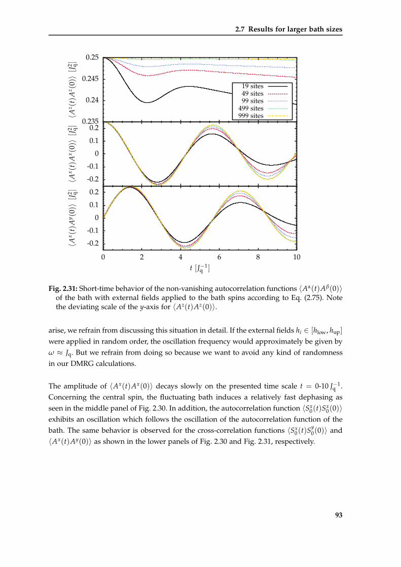
2.7 Results for larger bath sizes
0.235
0.24
0.245
0.25
〈Az(t)A
z(0)〉
[J2 q]
-0.2
-0.1
0
0.1
0.2
〈Ax(t)A
x(0)〉
[J2 q]
-0.2
-0.1
0
0.1
0.2
0 2 4 6 8 10
〈Ax(t)A
y(0)〉
[J2 q]
t [J−1q ]
19 sites49 sites99 sites
499 sites999 sites
Fig. 2.31: Short-time behavior of the non-vanishing autocorrelation functions 〈Aα(t)Aβ(0)〉of the bath with external fields applied to the bath spins according to Eq. (2.75). Notethe deviating scale of the y-axis for 〈Az(t)Az(0)〉.
arise, we refrain from discussing this situation in detail. If the external fields hi ∈ [hlow, hup]
were applied in random order, the oscillation frequency would approximately be given by
ω ≈ Jq. But we refrain from doing so because we want to avoid any kind of randomness
in our DMRG calculations.
The amplitude of 〈Ax(t)Ax(0)〉 decays slowly on the presented time scale t = 0-10 J−1q .
Concerning the central spin, the fluctuating bath induces a relatively fast dephasing as
seen in the middle panel of Fig. 2.30. In addition, the autocorrelation function 〈Sx0(t)S
x0(0)〉
exhibits an oscillation which follows the oscillation of the autocorrelation function of the
bath. The same behavior is observed for the cross-correlation functions 〈Sx0(t)S
y0(0)〉 and
〈Ax(t)Ay(0)〉 as shown in the lower panels of Fig. 2.30 and Fig. 2.31, respectively.
93
Chapter 2 Density Matrix Renormalization Group
0
0.05
0.1
0.15
0.2
0.25
〈Sz 0(
t)S
z 0(0)〉
0
0.05
0.1
0.15
0.2
〈Sx 0(t)S
x 0(0)〉
-0.04
-0.02
0
0.02
0.04
0 2 4 6 8 10
〈Sx 0(t)S
y 0(0)〉
t [J−1q ]
19 sites49 sites
99 sites499 sites
Fig. 2.32: Short-time behavior of the non-vanishing autocorrelation functions 〈Sα0(t)S
β0 (0)〉
of the central spin for a weak external field h0 = 0.2 Jq.
2.7.2.2 Field applied to central spin
The previously discussed scenario, where the external magnetic field was applied to the
bath spins only, does not reflect a situation occurring in experiment because the magnetic
field h0 acting on the central spin cannot be neglected. Furthermore, the Zeeman splitting
is much weaker for a nuclear spin than for an electron spin. Due to the large proton mass
mp, the ratio of the nuclear magneton µN and the Bohr magneton µB deviates significantly
from unity
µN
µB≈ me
mp≈ 10−3.
Hence, the field acting on the nuclear spins can be neglected while the influence of the
field h0 acting on the electron spin is crucial. In the following, the short-time behavior is
discussed for a weak, an intermediate, and a strong value of the field h0.
94
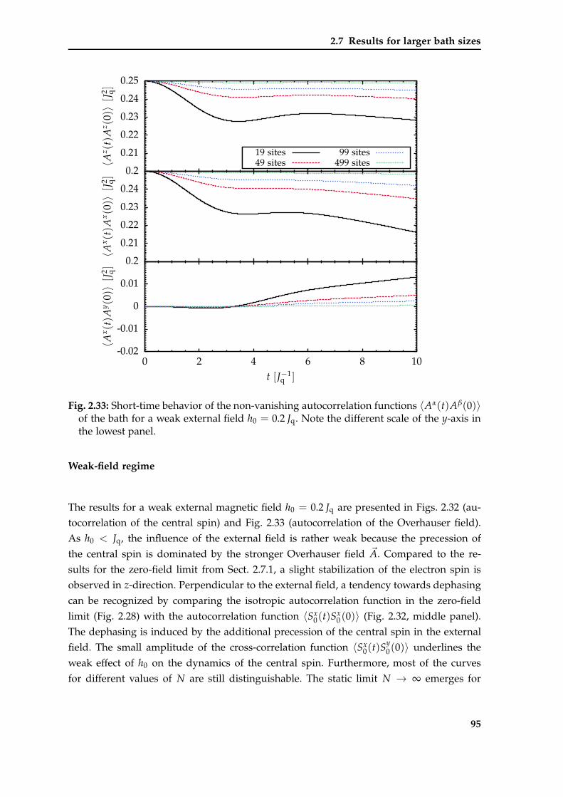
2.7 Results for larger bath sizes
0.2
0.21
0.22
0.23
0.24
0.25
〈Az(t)A
z(0)〉
[J2 q]
0.2
0.21
0.22
0.23
0.24
〈Ax(t)A
x(0)〉
[J2 q]
-0.02
-0.01
0
0.01
0 2 4 6 8 10
〈Ax(t)A
y(0)〉
[J2 q]
t [J−1q ]
19 sites49 sites
99 sites499 sites
Fig. 2.33: Short-time behavior of the non-vanishing autocorrelation functions 〈Aα(t)Aβ(0)〉of the bath for a weak external field h0 = 0.2 Jq. Note the different scale of the y-axis inthe lowest panel.
Weak-field regime
The results for a weak external magnetic field h0 = 0.2 Jq are presented in Figs. 2.32 (au-
tocorrelation of the central spin) and Fig. 2.33 (autocorrelation of the Overhauser field).
As h0 < Jq, the influence of the external field is rather weak because the precession of
the central spin is dominated by the stronger Overhauser field ~A. Compared to the re-
sults for the zero-field limit from Sect. 2.7.1, a slight stabilization of the electron spin is
observed in z-direction. Perpendicular to the external field, a tendency towards dephasing
can be recognized by comparing the isotropic autocorrelation function in the zero-field
limit (Fig. 2.28) with the autocorrelation function 〈Sx0(t)S
x0(0)〉 (Fig. 2.32, middle panel).
The dephasing is induced by the additional precession of the central spin in the external
field. The small amplitude of the cross-correlation function 〈Sx0(t)S
y0(0)〉 underlines the
weak effect of h0 on the dynamics of the central spin. Furthermore, most of the curves
for different values of N are still distinguishable. The static limit N → ∞ emerges for
95
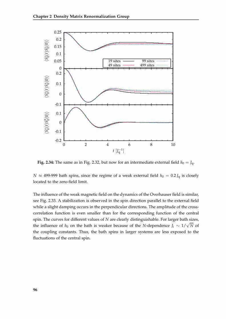
Chapter 2 Density Matrix Renormalization Group
0
0.05
0.1
0.15
0.2
0.25
〈Sz 0(
t)S
z 0(0)〉
-0.1
0
0.1
0.2
〈Sx 0(t)S
x 0(0)〉
-0.2
-0.1
0
0.1
0 2 4 6 8 10
〈Sx 0(t)S
y 0(0)〉
t [J−1q ]
19 sites49 sites
99 sites499 sites
Fig. 2.34: The same as in Fig. 2.32, but now for an intermediate external field h0 = Jq.
N ≈ 499-999 bath spins, since the regime of a weak external field h0 = 0.2 Jq is closely
located to the zero-field limit.
The influence of the weak magnetic field on the dynamics of the Overhauser field is similar,
see Fig. 2.33. A stabilization is observed in the spin direction parallel to the external field
while a slight damping occurs in the perpendicular directions. The amplitude of the cross-
correlation function is even smaller than for the corresponding function of the central
spin. The curves for different values of N are clearly distinguishable. For larger bath sizes,
the influence of h0 on the bath is weaker because of the N-dependence Ji ∼ 1/√
N of
the coupling constants. Thus, the bath spins in larger systems are less exposed to the
fluctuations of the central spin.
96
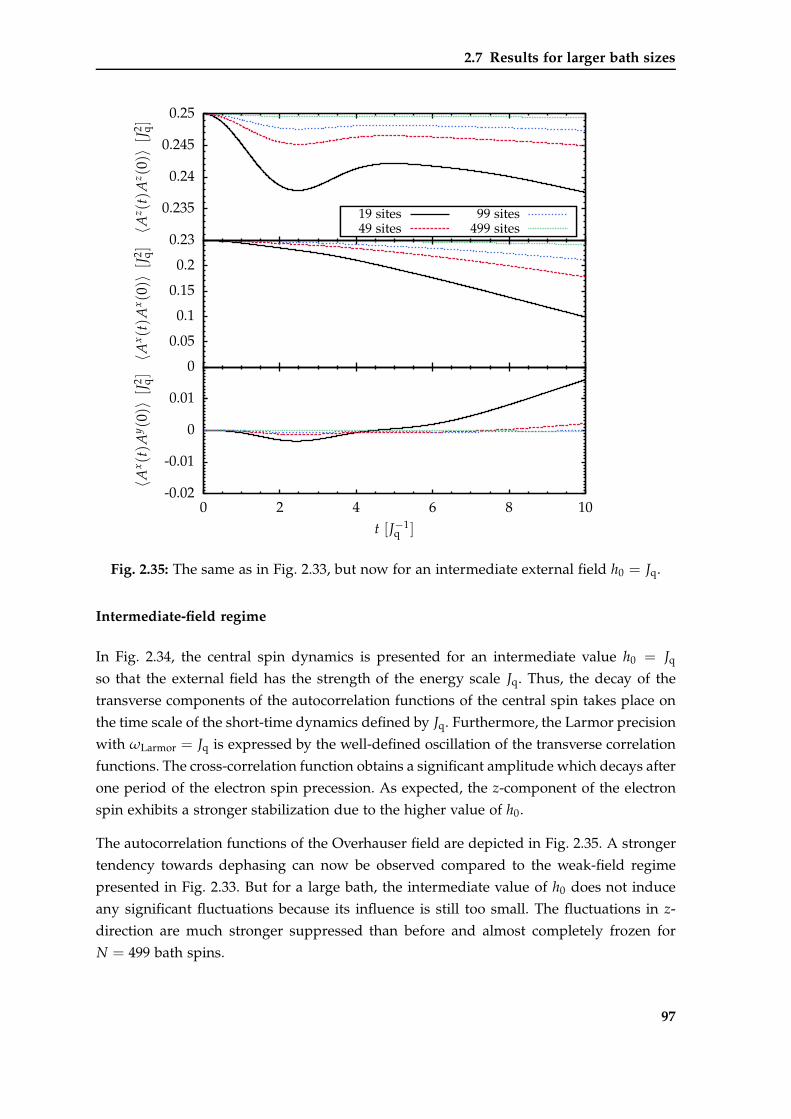
2.7 Results for larger bath sizes
0.23
0.235
0.24
0.245
0.25
〈Az(t)A
z(0)〉
[J2 q]
0
0.05
0.1
0.15
0.2
〈Ax(t)A
x(0)〉
[J2 q]
-0.02
-0.01
0
0.01
0 2 4 6 8 10
〈Ax(t)A
y(0)〉
[J2 q]
t [J−1q ]
19 sites49 sites
99 sites499 sites
Fig. 2.35: The same as in Fig. 2.33, but now for an intermediate external field h0 = Jq.
Intermediate-field regime
In Fig. 2.34, the central spin dynamics is presented for an intermediate value h0 = Jq
so that the external field has the strength of the energy scale Jq. Thus, the decay of the
transverse components of the autocorrelation functions of the central spin takes place on
the time scale of the short-time dynamics defined by Jq. Furthermore, the Larmor precision
with ωLarmor = Jq is expressed by the well-defined oscillation of the transverse correlation
functions. The cross-correlation function obtains a significant amplitude which decays after
one period of the electron spin precession. As expected, the z-component of the electron
spin exhibits a stronger stabilization due to the higher value of h0.
The autocorrelation functions of the Overhauser field are depicted in Fig. 2.35. A stronger
tendency towards dephasing can now be observed compared to the weak-field regime
presented in Fig. 2.33. But for a large bath, the intermediate value of h0 does not induce
any significant fluctuations because its influence is still too small. The fluctuations in z-
direction are much stronger suppressed than before and almost completely frozen for
N = 499 bath spins.
97
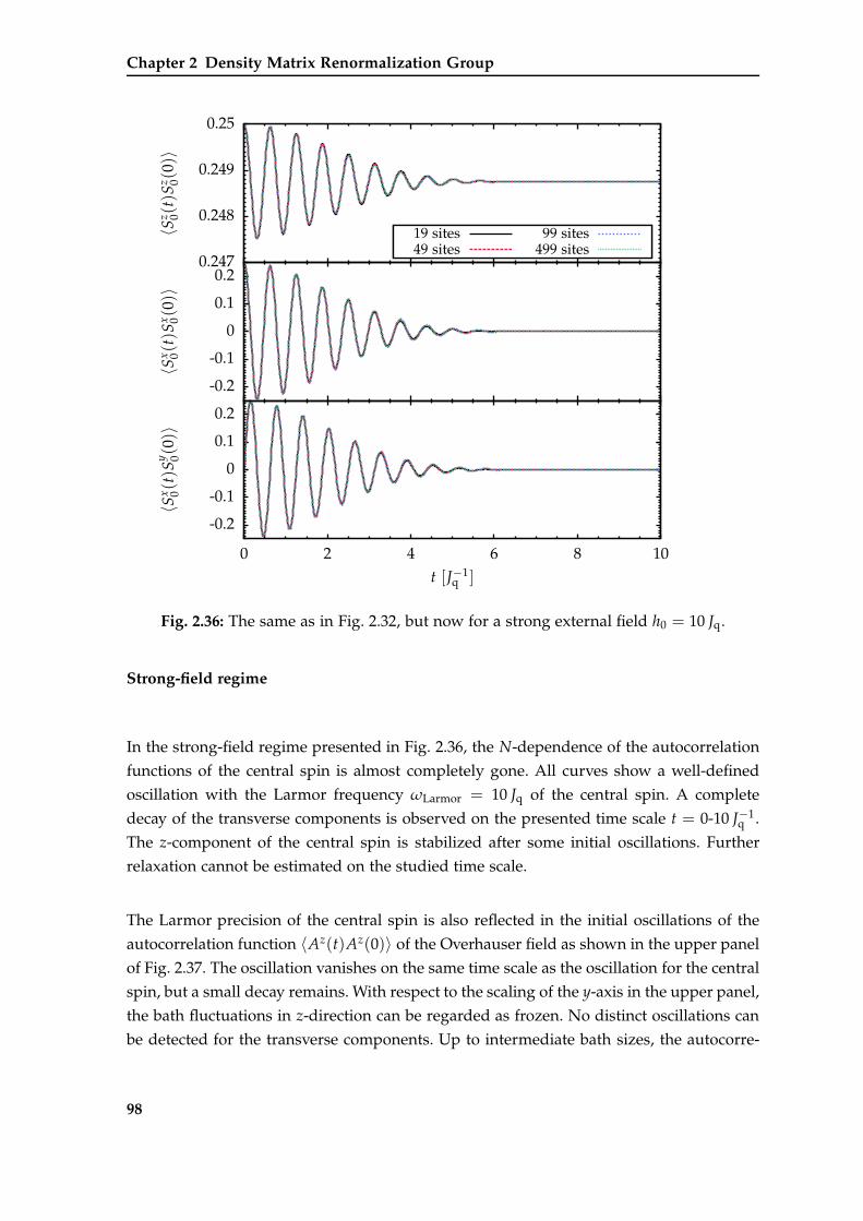
Chapter 2 Density Matrix Renormalization Group
0.247
0.248
0.249
0.25
〈Sz 0(
t)S
z 0(0)〉
-0.2
-0.1
0
0.1
0.2
〈Sx 0(t)S
x 0(0)〉
-0.2
-0.1
0
0.1
0.2
0 2 4 6 8 10
〈Sx 0(t)S
y 0(0)〉
t [J−1q ]
19 sites49 sites
99 sites499 sites
Fig. 2.36: The same as in Fig. 2.32, but now for a strong external field h0 = 10 Jq.
Strong-field regime
In the strong-field regime presented in Fig. 2.36, the N-dependence of the autocorrelation
functions of the central spin is almost completely gone. All curves show a well-defined
oscillation with the Larmor frequency ωLarmor = 10 Jq of the central spin. A complete
decay of the transverse components is observed on the presented time scale t = 0-10 J−1q .
The z-component of the central spin is stabilized after some initial oscillations. Further
relaxation cannot be estimated on the studied time scale.
The Larmor precision of the central spin is also reflected in the initial oscillations of the
autocorrelation function 〈Az(t)Az(0)〉 of the Overhauser field as shown in the upper panel
of Fig. 2.37. The oscillation vanishes on the same time scale as the oscillation for the central
spin, but a small decay remains. With respect to the scaling of the y-axis in the upper panel,
the bath fluctuations in z-direction can be regarded as frozen. No distinct oscillations can
be detected for the transverse components. Up to intermediate bath sizes, the autocorre-
98
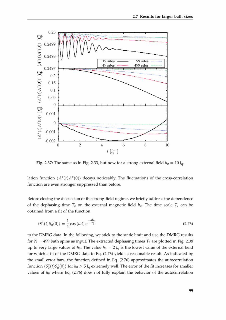
2.7 Results for larger bath sizes
0.2497
0.2498
0.2499
0.25
〈Az(t)A
z(0)〉
[J2 q]
0
0.05
0.1
0.15
0.2
〈Ax(t)A
x(0)〉
[J2 q]
-0.002
-0.001
0
0.001
0 2 4 6 8 10
〈Ax(t)A
y(0)〉
[J2 q]
t [J−1q ]
19 sites49 sites
99 sites499 sites
Fig. 2.37: The same as in Fig. 2.33, but now for a strong external field h0 = 10 Jq.
lation function 〈Ax(t)Ax(0)〉 decays noticeably. The fluctuations of the cross-correlation
function are even stronger suppressed than before.
Before closing the discussion of the strong-field regime, we briefly address the dependence
of the dephasing time T2 on the external magnetic field h0. The time scale T2 can be
obtained from a fit of the function
〈Sx0(t)S
x0(0)〉 =
14
cos (ωt) e− t2
2T22 (2.76)
to the DMRG data. In the following, we stick to the static limit and use the DMRG results
for N = 499 bath spins as input. The extracted dephasing times T2 are plotted in Fig. 2.38
up to very large values of h0. The value h0 = 2 Jq is the lowest value of the external field
for which a fit of the DMRG data to Eq. (2.76) yields a reasonable result. As indicated by
the small error bars, the function defined in Eq. (2.76) approximates the autocorrelation
function 〈Sx0(t)S
x0(0)〉 for h0 > 5 Jq extremely well. The error of the fit increases for smaller
values of h0 where Eq. (2.76) does not fully explain the behavior of the autocorrelation
99
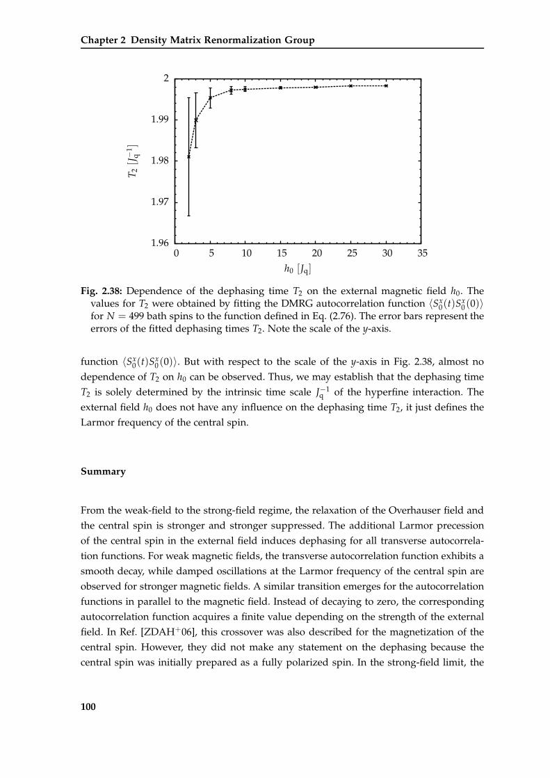
Chapter 2 Density Matrix Renormalization Group
1.96
1.97
1.98
1.99
2
0 5 10 15 20 25 30 35
T2[J−
1q
]
h0 [Jq]
Fig. 2.38: Dependence of the dephasing time T2 on the external magnetic field h0. Thevalues for T2 were obtained by fitting the DMRG autocorrelation function 〈Sx
0(t)Sx0(0)〉
for N = 499 bath spins to the function defined in Eq. (2.76). The error bars represent theerrors of the fitted dephasing times T2. Note the scale of the y-axis.
function 〈Sx0(t)S
x0(0)〉. But with respect to the scale of the y-axis in Fig. 2.38, almost no
dependence of T2 on h0 can be observed. Thus, we may establish that the dephasing time
T2 is solely determined by the intrinsic time scale J−1q of the hyperfine interaction. The
external field h0 does not have any influence on the dephasing time T2, it just defines the
Larmor frequency of the central spin.
Summary
From the weak-field to the strong-field regime, the relaxation of the Overhauser field and
the central spin is stronger and stronger suppressed. The additional Larmor precession
of the central spin in the external field induces dephasing for all transverse autocorrela-
tion functions. For weak magnetic fields, the transverse autocorrelation function exhibits a
smooth decay, while damped oscillations at the Larmor frequency of the central spin are
observed for stronger magnetic fields. A similar transition emerges for the autocorrelation
functions in parallel to the magnetic field. Instead of decaying to zero, the corresponding
autocorrelation function acquires a finite value depending on the strength of the external
field. In Ref. [ZDAH+06], this crossover was also described for the magnetization of the
central spin. However, they did not make any statement on the dephasing because the
central spin was initially prepared as a fully polarized spin. In the strong-field limit, the
100
2.7 Results for larger bath sizes
static limit N → ∞ already emerges in the autocorrelation functions of the central spin for
a small number of bath spins. As initially explained, the fluctuations of the Overhauser
field exhibit a N-dependence due to Ji ∼ 1/√
N.
A finite external field simplifies the DMRG calculations significantly. Due to the suppres-
sion of the relaxation in the spin direction parallel to external field, less states become im-
portant so that the total discarded weight is reduced. Compared to the zero-field limit, the
total discarded weight at t = 10 J−1q is at least one order of magnitude lower in the regime
of a strong external field. Moreover, a significant growth for larger times does not occur.
But there is also a substantial impact of the external field on the runtime of the DMRG
code. For strong external fields, a DMRG run for N = 499 bath spins up to t = 10 J−1q is
completed within a few hours compared to one to two days in the zero-field limit. The
enormous speedup has to be attributed to the dynamic adjustment of the number of kept
states.
101

Chapter 3
Classical Gaussian Fluctuations in the Zero-Field Limit
Contents
3.1 Motivation & introduction . . . . . . . . . . . . . . . . . . . . . . . . . . . 104
3.2 Average Hamiltonian theory . . . . . . . . . . . . . . . . . . . . . . . . . . 105
3.3 Comparison with DMRG . . . . . . . . . . . . . . . . . . . . . . . . . . . . 108
3.4 Optimization of the numerical simulation . . . . . . . . . . . . . . . . . . 111
3.4.1 Conservation of the total spin . . . . . . . . . . . . . . . . . . . . . . 1123.4.2 Classical treatment of the central spin . . . . . . . . . . . . . . . . . 1153.4.3 Discussion . . . . . . . . . . . . . . . . . . . . . . . . . . . . . . . . . 117
3.5 Remarks on finite external magnetic fields . . . . . . . . . . . . . . . . . . 120
In the previous chapter, the numerical treatment of the central spin model (1.4) in the
framework of DMRG was presented. Thereby, we gained access to relatively large spin
baths consisting of up to N ≈ 1000 spins. But reachable times are limited to t ≈ 30-
50 J−1q because of the accumulating discarded weight and the growing entanglement in
the system.
Now, we take one step back from the heavy numerical treatment with DMRG and con-
sult an effective semiclassical picture for the dynamics of the central spin. To this end, we
first motivate the approximation of the bath by a classical random field in Sect. 3.1. The
semiclassical model is studied by numerical simulation and on the basis of average Hamil-
tonian theory (AHT). The latter is derived in leading order in Sect. 3.2. In Sect. 3.3, we
demonstrate that the dynamics of the central spin is indeed captured well by the semiclas-
sical model for a large number of bath spins up to intermediate times. But the comparison
with DMRG and AHT reveals that there is still room for improving the numerical simula-
tion of the semiclassical model. Hence, the separate treatment of the conserved total spin
as well as the classical treatment of the central spin is addressed in Sect. 3.4. The present
discussion of the semiclassical model is solely restricted to the zero-field limit. In Sect. 3.5,
a short remark concerning the semiclassical model in finite external fields is made.
103
Chapter 3 Classical Gaussian Fluctuations in the Zero-Field Limit
3.1 Motivation & introduction
For the zero-field limit discussed in Sect. 2.7.1, the DMRG results revealed a fast con-
vergence of the autocorrelation functions and an almost static bath already for moderate
numbers of bath spins. This is a strong hint that quantum fluctuations play only a mi-
nor role in the bath. The classical character of the bath achieves further backup by the
following simple analytic argument. We regard the square of an operator norm
Tr(
Aα)2
=14
N
∑i=1
J2i =
J2q
4(3.1a)
where the operator Aα represents the component α of the Overhauser field as defined in
Eq. (1.5a). Obviously, one concludes that Aα = O(1) if the coupling constants are scaled
as motivated in Sect. 1.4. But for the commutator we find
Tr([
Aα, Aβ])2
=14
N
∑i=1
J4i ∝
14
N
∑i=1
(J2q
N
)2
=14
J4q
N. (3.1b)
This implies that the norm of the commutator vanishes in the limit N → ∞ because
[Aα, Aβ] = O(J2q/
√N). Hence, the bath can be regarded as a classical variable for a large
number of bath spins. This is well described by the Hamiltonian
Hsc = ~η (t) · ~S0, (3.2)
where an electron spin-1/2 interacts with a classical random field ~η(t).
The semiclassical model in Eq. (3.2) is derived from the central spin model (1.5) by replac-
ing the quantum bath ~A by a classical fluctuating field ~η(t). Thereby, back-action effects
of the central spin on the fluctuations of the Overhauser field are neglected. According to
the central limit theorem, the bath obeys Gaussian statistics because it consists of a large
number of independent two-level fluctuations. Thus, the fluctuations are fully defined by
their autocorrelation function
gαβ (t1 − t2) = ηα (t1) ηβ (t2) (3.3a)
and their mean value
η (t) = 0. (3.3b)
Without loss of generality, it is set to zero because a finite mean value only creates a
constant offset.
104
3.2 Average Hamiltonian theory
When comparing the semiclassical model to the quantum model, the correlation function
gαβ(t) of the gaussian noise is identified with the autocorrelation 〈Aα(t)Aβ(0)〉 of the
Overhauser field. In the present chapter, we focus on the zero-field limit where all non-
diagonal correlations vanish and all diagonal correlations are isotropic: g(t) ≡ gαα(t), see
Sect. 2.7.1 for comparison.
The investigation of a semiclassical model for the central spin problem, where the bath is
replaced by an effective field, was already addressed before [MER02, EN04]. In a recent
preprint by Witzel et al. [WYD13], a semiclassical approximation was applied to the spin
bath in the strong-field limit. The correlation function of the bath was obtained from a
correlated cluster expansion [YL08a, YL09, WCCDS12]. Due to the strong external field,
spin flips between central spin and bath were neglected. The decoherence was induced by
spectral diffusion, which is typical for cluster expansions, see Sect. 1.5.2 for details. Hence,
their semiclassical ansatz only comprised dephasing, the relaxation of the central spin was
excluded.
3.2 Average Hamiltonian theory
We begin with an analytical investigation of the semiclassical model in the zero-field limit
on the level of average Hamiltonian theory. For a time-dependent Hamiltonian, the ana-
lytical evaluation of the time-evolution operator
U (t) = T exp
−i
t∫
0
dt′ H(t′)
, (3.4)
in a closed form is usually impossible due to the time-ordering expressed by the opera-
tor T . To simplify the time-evolution operator, we apply the Magnus expansion [Mag54,
BCOR09] which enables a systematic analytical treatment of Eq. (3.4). In leading order, the
time-ordering in Eq. (3.4) is simply neglected. The approximation
U (t) ≈ exp
−i
t∫
0
dt′ H(t′)
(3.5)
is certainly justified if the Hamiltonian is almost static or if it fluctuates very quickly.
For the semiclassical picture, a static Hamiltonian corresponds to a constant correlation
function of the noise. This is well supported by the DMRG results for the zero-field limit
105
Chapter 3 Classical Gaussian Fluctuations in the Zero-Field Limit
discussed in Sect. 2.7.1. The operator Aα (1.5a) representing the Overhauser field contains
all local operators of the bath and the corresponding autocorrelation function is nearly
constant, see Fig. 2.29 for details.
By exploiting the properties of the Pauli matrices and the spherical symmetry of the fluc-
tuations in the zero-field limit, the time-evolution operator (3.5) is rewritten in the form
U (t) = cosv
2· 1− i sin
v
2· σ~v (3.6)
where the vector
~v :=t∫
0
dt′~η(t′) (3.7)
stands for the leading order of the Magnus expansion. It contains the complete time de-
pendence. The operator
σ~v =~σ ·~v∣∣~v∣∣
= sin θ cos ϕ σx + sin θ sin ϕ σy + cos θ σz
(3.8)
is the projection of the Pauli matrices along the direction of ~v. Here, the angles ϕ and θ
originate from the representation of ~v in spherical coordinates. The simplified form of the
time-evolution operator (3.6) is used to calculate the autocorrelation function
〈Sz0(t)S
z0(0)〉 =
18
Tr[U† (t) σzU (t) σz
](3.9)
of the central spin. After some straightforward simplifications, it takes the form
〈Sz0 (t) Sz
0 (0)〉 =14
[cos2 v
2+ sin2 v
2
(2 cos2 θ − 1
)](3.10)
prior to averaging over v. Next, the average with respect to θ and v has to be carried
out. Because of the spin rotational symmetry, the average over the angle θ simply yields
cos2 θ = 1/3. The remaining contribution
〈Sz0 (t) Sz
0 (0)〉 =14
(13+
23
cos v
)(3.11)
is averaged with respect to the Gaussian distribution
p (v) =1√
2π Var v(t)e−
v22 Var v(t) (3.12)
106
3.2 Average Hamiltonian theory
of the fluctuations. After all integrations have been carried out analytically, the final result
for the autocorrelation function of the central spin is given as
〈Sz0 (t) Sz
0 (0)〉 =16
[(1 − Var v (t)
)e−
Var v(t)2 +
12
], (3.13)
where the time dependence resides in the variance Var v(t) = (∫ t
0 dt′ η(t′))2. It is related
to the autocorrelation function of the random noise
Var v (t) = 2t∫
0
dt1
t1∫
0
dt2 g (t1 − t2) . (3.14)
For the beginning, we discuss a constant autocorrelation function g(t) = J2q/4 valid in the
limit N → ∞, see Fig. 2.29. Then, the variance Var v(t) = t2 J2q/4 increases quadratically
in time and the autocorrelation function of the central spin in leading order of our AHT
reads
〈Sz0 (t) Sz
0 (0)〉 =16
e−
t2 J2q
8
1 −
t2 J2q
4
+
12
. (3.15)
This result is identical to the one obtained by Merkulov et al. [MER02] which was de-
rived from a classical discussion of the static spin bath. Our AHT for the semiclassical
model (3.2) has the merit to be based on the Magnus expansion and can be extended sys-
tematically to higher orders in nested commutators [BCOR09]. But note that there are no
corrections in higher order for a static autocorrelation function. Furthermore, the corre-
lation function g(t) of the fluctuations enters in the general expression for 〈Sz0(t)S
z0(0)〉
from Eq. (3.13) via the variance Var v(t). Hence, the results can easily be adapted to ar-
bitrary correlation functions g(t). They do not necessarily have to be given by an analytic
expression, numerical results for g(t) are also legitimate. For example, this may comprise
autocorrelation functions obtained from DMRG or experimental results. There, one usu-
ally measures the spectrum of the bath which is linked to the real-time correlation function
by Fourier transform. We highlight that independently of the actual time dependence of
Var v(t), the autocorrelation function in Eq. 3.13 always converges to a plateau of 1/12 as
long as Var v(t) diverges monotonically in time.
Finally, we verify our AHT result by a numerical simulation of the semiclassical model. As
we are dealing with a two-level system, the integration is carried out easily. A reduction
of the integration error for time-dependent Hamiltonians is achieved by commutator-free
exponential time propagators (CFETs) as introduced by Alvermann et al. [AF11, AFL12].
The additional numerical effort is negligible because an exact analytical representation
of the time-evolution operator of a two-level system is available. Hence, no additional
107
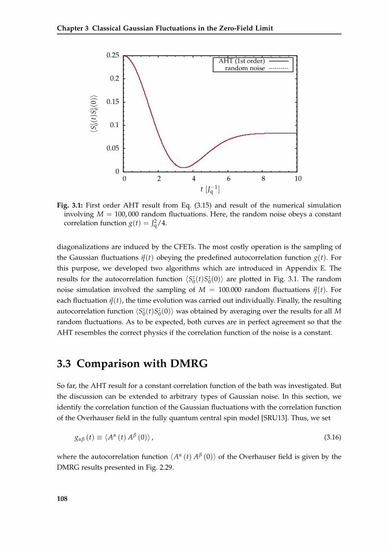
Chapter 3 Classical Gaussian Fluctuations in the Zero-Field Limit
0
0.05
0.1
0.15
0.2
0.25
0 2 4 6 8 10
〈Sz 0(
t)S
z 0(0)〉
t [J−1q ]
AHT (1st order)random noise
Fig. 3.1: First order AHT result from Eq. (3.15) and result of the numerical simulationinvolving M = 100, 000 random fluctuations. Here, the random noise obeys a constantcorrelation function g(t) = J2
q/4.
diagonalizations are induced by the CFETs. The most costly operation is the sampling of
the Gaussian fluctuations ~η(t) obeying the predefined autocorrelation function g(t). For
this purpose, we developed two algorithms which are introduced in Appendix E. The
results for the autocorrelation function 〈Sz0(t)S
z0(0)〉 are plotted in Fig. 3.1. The random
noise simulation involved the sampling of M = 100.000 random fluctuations ~η(t). For
each fluctuation ~η(t), the time evolution was carried out individually. Finally, the resulting
autocorrelation function 〈Sz0(t)S
z0(0)〉 was obtained by averaging over the results for all M
random fluctuations. As to be expected, both curves are in perfect agreement so that the
AHT resembles the correct physics if the correlation function of the noise is a constant.
3.3 Comparison with DMRG
So far, the AHT result for a constant correlation function of the bath was investigated. But
the discussion can be extended to arbitrary types of Gaussian noise. In this section, we
identify the correlation function of the Gaussian fluctuations with the correlation function
of the Overhauser field in the fully quantum central spin model [SRU13]. Thus, we set
gαβ (t) ≡ 〈Aα (t) Aβ (0)〉 , (3.16)
where the autocorrelation function 〈Aα (t) Aβ (0)〉 of the Overhauser field is given by the
DMRG results presented in Fig. 2.29.
108
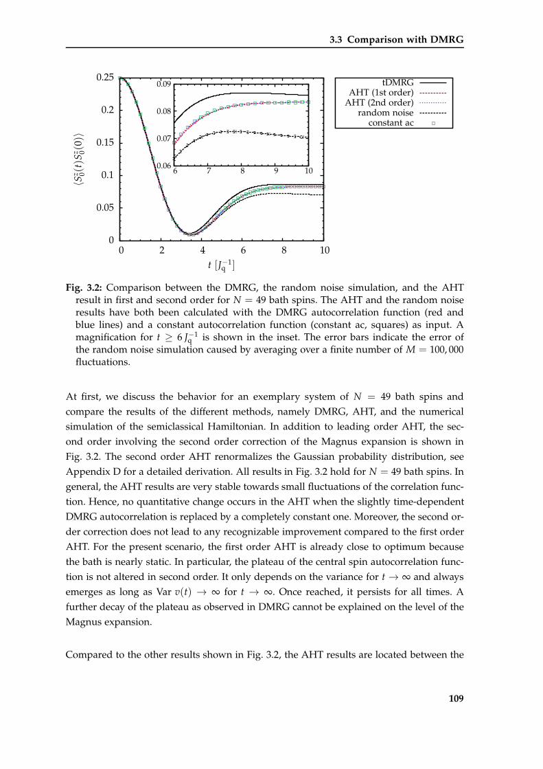
3.3 Comparison with DMRG
0
0.05
0.1
0.15
0.2
0.25
0 2 4 6 8 10
〈Sz 0(
t)S
z 0(0)〉
t [J−1q ]
0.06
0.07
0.08
0.09
6 7 8 9 10
tDMRGAHT (1st order)
AHT (2nd order)random noise
constant ac
Fig. 3.2: Comparison between the DMRG, the random noise simulation, and the AHTresult in first and second order for N = 49 bath spins. The AHT and the random noiseresults have both been calculated with the DMRG autocorrelation function (red andblue lines) and a constant autocorrelation function (constant ac, squares) as input. Amagnification for t ≥ 6 J−1
q is shown in the inset. The error bars indicate the error ofthe random noise simulation caused by averaging over a finite number of M = 100, 000fluctuations.
At first, we discuss the behavior for an exemplary system of N = 49 bath spins and
compare the results of the different methods, namely DMRG, AHT, and the numerical
simulation of the semiclassical Hamiltonian. In addition to leading order AHT, the sec-
ond order involving the second order correction of the Magnus expansion is shown in
Fig. 3.2. The second order AHT renormalizes the Gaussian probability distribution, see
Appendix D for a detailed derivation. All results in Fig. 3.2 hold for N = 49 bath spins. In
general, the AHT results are very stable towards small fluctuations of the correlation func-
tion. Hence, no quantitative change occurs in the AHT when the slightly time-dependent
DMRG autocorrelation is replaced by a completely constant one. Moreover, the second or-
der correction does not lead to any recognizable improvement compared to the first order
AHT. For the present scenario, the first order AHT is already close to optimum because
the bath is nearly static. In particular, the plateau of the central spin autocorrelation func-
tion is not altered in second order. It only depends on the variance for t → ∞ and always
emerges as long as Var v(t) → ∞ for t → ∞. Once reached, it persists for all times. A
further decay of the plateau as observed in DMRG cannot be explained on the level of the
Magnus expansion.
Compared to the other results shown in Fig. 3.2, the AHT results are located between the
109
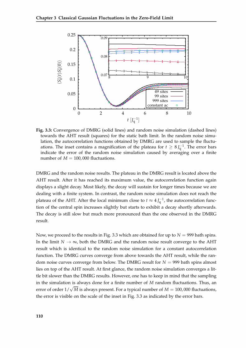
Chapter 3 Classical Gaussian Fluctuations in the Zero-Field Limit
0
0.05
0.1
0.15
0.2
0.25
0 2 4 6 8 10
〈Sz 0(
t)S
z 0(0)〉
t [J−1q ]
0.07
0.08
0.09
8 9 10
49 sites99 sites
999 sitesconstant ac
Fig. 3.3: Convergence of DMRG (solid lines) and random noise simulation (dashed lines)towards the AHT result (squares) for the static bath limit. In the random noise simu-lation, the autocorrelation functions obtained by DMRG are used to sample the fluctu-ations. The inset contains a magnification of the plateau for t ≥ 8 J−1
q . The error barsindicate the error of the random noise simulation caused by averaging over a finitenumber of M = 100, 000 fluctuations.
DMRG and the random noise results. The plateau in the DMRG result is located above the
AHT result. After it has reached its maximum value, the autocorrelation function again
displays a slight decay. Most likely, the decay will sustain for longer times because we are
dealing with a finite system. In contrast, the random noise simulation does not reach the
plateau of the AHT. After the local minimum close to t ≈ 4 J−1q , the autocorrelation func-
tion of the central spin increases slightly but starts to exhibit a decay shortly afterwards.
The decay is still slow but much more pronounced than the one observed in the DMRG
result.
Now, we proceed to the results in Fig. 3.3 which are obtained for up to N = 999 bath spins.
In the limit N → ∞, both the DMRG and the random noise result converge to the AHT
result which is identical to the random noise simulation for a constant autocorrelation
function. The DMRG curves converge from above towards the AHT result, while the ran-
dom noise curves converge from below. The DMRG result for N = 999 bath spins almost
lies on top of the AHT result. At first glance, the random noise simulation converges a lit-
tle bit slower than the DMRG results. However, one has to keep in mind that the sampling
in the simulation is always done for a finite number of M random fluctuations. Thus, an
error of order 1/√
M is always present. For a typical number of M = 100, 000 fluctuations,
the error is visible on the scale of the inset in Fig. 3.3 as indicated by the error bars.
110
3.4 Optimization of the numerical simulation
The convergence towards the AHT result is expected because the bath becomes more and
more static with increasing number of bath spins. To our knowledge, it is the first time
that the systematic convergence has been demonstrated. This has to be attributed to DMRG
which is capable of treating fairly large system sizes where the convergence sets in. Along
with the analytical argument presented Sect. 3.1, our results prove that the bath behaves
classically already for a moderate number of bath spins. The convergence in the short-
time behavior is observed for O(1000) bath spins, which is roughly one to two orders
of magnitudes smaller than the typical number of nuclear spins interacting with a single
electron spin confined in a quantum dot, see Sect. 1.3.
So far, our discussion is restricted to the short time behavior. Recent comparisons between
the static bath approximation [MER02] and a combination of Bethe ansatz and Monte
Carlo techniques [FS13b] revealed a stronger influence of quantum fluctuations on longer
time scales expressed by a fractional decay of the plateau. But the numerical investigation
of the central spin model was limited to N = 48 bath spins at most so that a conclusion
for large baths cannot be drawn. According to Ref. [MER02], the reduction of the plateau
by a certain fraction is due to fluctuations in the nuclear spin bath. However, the complete
impact of these back-actions effects occurs on a time scale which is not fully captured by
DMRG and consequently not by our semiclassical approach which uses the DMRG output
for the fluctuations of the Overhauser field as input.
3.4 Optimization of the numerical simulation
The curves from Fig. 3.3 revealed that the plateau 〈Sz0(t)S
z0(0)〉 = 1/12 arises in the random
noise simulation only when the bath fluctuations are completely frozen. As long as the
correlation function of the noise exhibits a marginal decay, the exact value of this plateau is
not reached. Moreover, the autocorrelation function of the central spin in the semiclassical
picture always displays a decay, even if the correlations decay on very long time scales.
The neglect of conservation laws of the full quantum model in the semiclassical treatment
is one reason for this behavior.
A well-known example for a conserved quantity in the central spin model is the total
spin
~I =N
∑i=0
~Si. (3.17)
111
Chapter 3 Classical Gaussian Fluctuations in the Zero-Field Limit
The DMRG captures the conservation of the total spin as well as all other conservation
laws in the central spin model numerically exact. However, this statement does not hold
for the semiclassical model as defined in Eq. (3.2).
3.4.1 Conservation of the total spin
In this section, we present how the conservation of the total spin ~I can be incorporated
into the semiclassical model. Therefore, we study the slightly modified Hamiltonian
H′ = ~S0
N
∑i=0
Ji~Si (3.18)
for the quantum central spin model. The central spin ~S0 has been included in the sum
which was restricted to the bath spins originally. The new contribution induces a constant
shift = 3J0/4 in the Hamiltonian for S = 1/2. Thus, it has no influence on the relevant
physics of the model. The mean value of all couplings is assigned to the coupling constant
of the central spin
J0 :=1N
N
∑i=1
Ji. (3.19)
Consequently, the fluctuating field
~A =N
∑i=0
Ji~Si (3.20a)
now comprises the central spin ~S0 in addition to the bath spins. To take the conservation
of the total spin into account, we rewrite it in the form
~A = ~A0 + ∆~A. (3.20b)
The part
~A0 = J0~I (3.21a)
is constant and conserved, while the contribution
∆~A =N
∑i=1
(Ji − J0) ~Si (3.21b)
112
3.4 Optimization of the numerical simulation
contains the fluctuating part. The separation into two contributions respects the conserved
total momentum because the fluctuating part ∆~A is always perpendicular to the constant
part ~A0, see below. Additionally, the separation is well supported by the results for the
quantum model: The correlation function of the bath (see Fig. 2.29) is nearly a constant
only modulated by some weak fluctuations on top.
With ~A0(t) = ~A0(0), one deduces immediately that the correlation function of the con-
served part is given by the constant expression
〈Aα0 (t) A
β0 (0)〉 = J2
0N + 1
4δαβ. (3.22a)
We still stick to the isotropic model, but use a general notation so that the present dis-
cussion can easily be extended to other symmetries. Moreover, the conserved and the
fluctuating part are independent at all times
〈Aα0 (t) ∆A
β0 (0)〉 = 〈Aα
0 (0) ∆Aβ0 (0)〉
=J0
4δαβ
N
∑i=0
(Ji − J0) = 0.(3.22b)
Thus, the autocorrelation function of the field ~A acquires the form
gαβ (t) = J20
N + 14
δαβ + ∆gαβ (t) (3.23)
with
∆gαβ (t) := 〈∆Aα (t) ∆Aβ (0)〉 . (3.24)
Next, we address the central spin ~S0 which is treated similarly to the field ~A
~S0 =1
N + 1~I + ∆~S0, (3.25)
where the fluctuating part reads
∆~S0 =N
N + 1~S0 −
1N + 1
N
∑i=1
~Si (3.26)
and the fraction ~I/(N + 1) of the total spin ~I (3.17) is the constant contribution. Like for~A, there is no correlation between the constant and the fluctuating part
〈Iα (t)∆Sβ0 (0)〉 = 〈Iα (0) ∆S
β0 (0)〉
=14
N
N + 1− N
14
1N + 1
= 0.(3.27)
113
Chapter 3 Classical Gaussian Fluctuations in the Zero-Field Limit
Consequently, the autocorrelation function of the central spin ~S0 is given by
〈Sα0 (t) S
β0 (0)〉 = δαβ
14
1N + 1
+ ∆cαβ (t) (3.28)
with
∆cαβ (t) := 〈∆Sα0 (t) ∆S
β0 (0)〉 . (3.29)
In this way, the conserved part has been separated from the fluctuating part for both the
central spin and the operator ~A. We incorporate this concept into the semiclassical model
by regarding the Hamiltonian
H′sc = ~η (t) · ∆~S0 (3.30a)
which only treats the fluctuating part of the central spin. Since the conserved part is a
constant, it does not enter in the latter Hamiltonian. As before, the fluctuating field ~η(t) is a
random Gaussian variable. But its correlation function is defined by gαβ(t) from Eq. (3.23)
involving the separate treatment of the fluctuating and the conserved part of ~A from
Eq. (3.20b). By inserting the expression for ∆~S0 in Eq. (3.30a), the semiclassical Hamiltonian
may be written as
H′sc =
N
∑i=0
hi (3.30b)
where
h0 :=N
N + 1~η (t) · ~S0 (3.31a)
hi := − 1N + 1
~η (t) · ~Si, i ∈ 1, 2, . . . , N . (3.31b)
Hence, the time evolution of the bath spins ~Si is completely independent and the fluc-
tuating part ∆cαβ (t) of the autocorrelation function of the central spin can be calculated
by
∆cαβ (t) =
(N
N + 1
)2
∆c(0)αβ (t) +
N
(N + 1)2 ∆c(i)αβ (t) (3.32)
with the two independent contributions
∆c(0)αβ (t) := 〈Sα
0 (t) Sβ0 (0)〉 with h0 from Eq. (3.31a) (3.33a)
∆c(i)αβ (t) := 〈Sα
i (t) Sβi (0)〉 with hi from Eq. (3.31b). (3.33b)
114
3.4 Optimization of the numerical simulation
In total, two independent runs of the code are required for simulating the semiclassi-
cal model including the conservation of the total spin. The run with the Hamiltonian h0
involves the strong coupling N/(N + 1) between central spin and bath. Thus, the contri-
bution ∆c(0)αβ (t) dominates the dynamics of the autocorrelation function 〈Sα
0 (t) Sβ0 (0)〉. In
contrast, the coupling −1/(N + 1) between a single bath spin ~Si and ~η(t) is very small.
Consequently, the Hamiltonian hi induces only a very weak dynamics which hardly has
an impact on the discussed time scales.
The separate treatment of the conserved total spin leads to a stabilization of the plateau
observed for intermediate time scales. The stabilization depends on the number of bath
spins N. In Sect. 3.4.3, we present the numerical results up to intermediate time scales and
discuss the improvement compared to the plain numerical simulation of the semiclassical
model.
3.4.2 Classical treatment of the central spin
In the above introduced modification of the random noise simulation, the central spin is
still treated on the quantum level while the bath is a classical variable. However, the pre-
cession of a quantum spin-1/2 is identical to the one of a classical vector in R3, see for
instance Ref. [MER02]. This is due to the local isomorphism between the rotation group
SO(3) of all rotations in a three-dimensional real vector space and the group SU(2) of
complex rotations, see below. Furthermore, the equations of motion of a spin in a field
are linear so that it does not matter whether one follows the operators or the expectation
values. Thus, the question arises how the classical treatment of the central spin affects the
numerical simulation of the semiclassical model. Outgoing from the optimized simula-
tion including the conservation of the total spin, we now address the central spin on the
classical level.
We recall the semiclassical Hamiltonian of Eq. (3.30a) and insert the expression for the
fluctuating part ∆~S0 of the central spin defined by Eq. (3.25)
Hsc = ~η (t)
(~S0 −
1N + 1
~I
). (3.34)
According to Eq. (3.20b), the Gaussian fluctuation ~η(t) can be written as
~η (t) = J0~I + ∆~η (t) . (3.35)
115
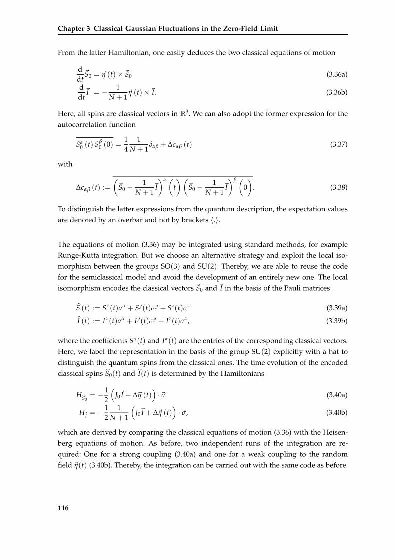
Chapter 3 Classical Gaussian Fluctuations in the Zero-Field Limit
From the latter Hamiltonian, one easily deduces the two classical equations of motion
ddt
~S0 = ~η (t)× ~S0 (3.36a)
ddt~I = − 1
N + 1~η (t)×~I. (3.36b)
Here, all spins are classical vectors in R3. We can also adopt the former expression for the
autocorrelation function
Sα0 (t) S
β0 (0) =
14
1N + 1
δαβ + ∆cαβ (t) (3.37)
with
∆cαβ (t) :=(~S0 −
1N + 1
~I
)α (t
)(~S0 −
1N + 1
~I
)β (0)
. (3.38)
To distinguish the latter expressions from the quantum description, the expectation values
are denoted by an overbar and not by brackets 〈.〉.
The equations of motion (3.36) may be integrated using standard methods, for example
Runge-Kutta integration. But we choose an alternative strategy and exploit the local iso-
morphism between the groups SO(3) and SU(2). Thereby, we are able to reuse the code
for the semiclassical model and avoid the development of an entirely new one. The local
isomorphism encodes the classical vectors ~S0 and ~I in the basis of the Pauli matrices
S (t) := Sx(t)σx + Sy(t)σy + Sz(t)σz (3.39a)
I (t) := Ix(t)σx + Iy(t)σy + Iz(t)σz, (3.39b)
where the coefficients Sα(t) and Iα(t) are the entries of the corresponding classical vectors.
Here, we label the representation in the basis of the group SU(2) explicitly with a hat to
distinguish the quantum spins from the classical ones. The time evolution of the encoded
classical spins S0(t) and I(t) is determined by the Hamiltonians
HS0= −1
2
(J0~I + ∆~η (t)
)·~σ (3.40a)
HI = −12
1N + 1
(J0~I + ∆~η (t)
)·~σ, (3.40b)
which are derived by comparing the classical equations of motion (3.36) with the Heisen-
berg equations of motion. As before, two independent runs of the integration are re-
quired: One for a strong coupling (3.40a) and one for a weak coupling to the random
field ~η(t) (3.40b). Thereby, the integration can be carried out with the same code as before.
116
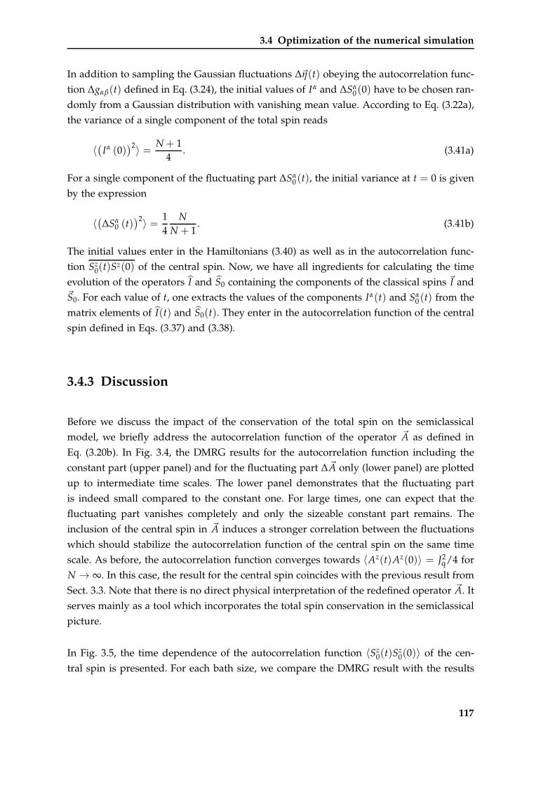
3.4 Optimization of the numerical simulation
In addition to sampling the Gaussian fluctuations ∆~η(t) obeying the autocorrelation func-
tion ∆gαβ(t) defined in Eq. (3.24), the initial values of Iα and ∆Sα0(0) have to be chosen ran-
domly from a Gaussian distribution with vanishing mean value. According to Eq. (3.22a),
the variance of a single component of the total spin reads
〈(
Iα (0))2〉 = N + 1
4. (3.41a)
For a single component of the fluctuating part ∆Sα0(t), the initial variance at t = 0 is given
by the expression
〈(∆Sα
0 (t))2〉 = 1
4N
N + 1. (3.41b)
The initial values enter in the Hamiltonians (3.40) as well as in the autocorrelation func-
tion Sz0(t)S
z(0) of the central spin. Now, we have all ingredients for calculating the time
evolution of the operators I and S0 containing the components of the classical spins ~I and~S0. For each value of t, one extracts the values of the components Iα(t) and Sα
0(t) from the
matrix elements of I(t) and S0(t). They enter in the autocorrelation function of the central
spin defined in Eqs. (3.37) and (3.38).
3.4.3 Discussion
Before we discuss the impact of the conservation of the total spin on the semiclassical
model, we briefly address the autocorrelation function of the operator ~A as defined in
Eq. (3.20b). In Fig. 3.4, the DMRG results for the autocorrelation function including the
constant part (upper panel) and for the fluctuating part ∆~A only (lower panel) are plotted
up to intermediate time scales. The lower panel demonstrates that the fluctuating part
is indeed small compared to the constant one. For large times, one can expect that the
fluctuating part vanishes completely and only the sizeable constant part remains. The
inclusion of the central spin in ~A induces a stronger correlation between the fluctuations
which should stabilize the autocorrelation function of the central spin on the same time
scale. As before, the autocorrelation function converges towards 〈Az(t)Az(0)〉 = J2q/4 for
N → ∞. In this case, the result for the central spin coincides with the previous result from
Sect. 3.3. Note that there is no direct physical interpretation of the redefined operator ~A. It
serves mainly as a tool which incorporates the total spin conservation in the semiclassical
picture.
In Fig. 3.5, the time dependence of the autocorrelation function 〈Sz0(t)S
z0(0)〉 of the cen-
tral spin is presented. For each bath size, we compare the DMRG result with the results
117
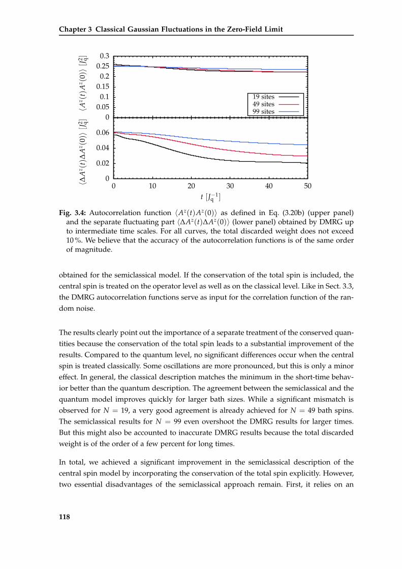
Chapter 3 Classical Gaussian Fluctuations in the Zero-Field Limit
00.050.1
0.150.2
0.250.3
〈Az(t)A
z(0)〉
[J2 q]
0
0.02
0.04
0.06
0 10 20 30 40 50〈∆A
z(t)∆
Az(0)〉
[J2 q]
t [J−1q ]
19 sites49 sites99 sites
Fig. 3.4: Autocorrelation function 〈Az(t)Az(0)〉 as defined in Eq. (3.20b) (upper panel)and the separate fluctuating part 〈∆Az(t)∆Az(0)〉 (lower panel) obtained by DMRG upto intermediate time scales. For all curves, the total discarded weight does not exceed10 %. We believe that the accuracy of the autocorrelation functions is of the same orderof magnitude.
obtained for the semiclassical model. If the conservation of the total spin is included, the
central spin is treated on the operator level as well as on the classical level. Like in Sect. 3.3,
the DMRG autocorrelation functions serve as input for the correlation function of the ran-
dom noise.
The results clearly point out the importance of a separate treatment of the conserved quan-
tities because the conservation of the total spin leads to a substantial improvement of the
results. Compared to the quantum level, no significant differences occur when the central
spin is treated classically. Some oscillations are more pronounced, but this is only a minor
effect. In general, the classical description matches the minimum in the short-time behav-
ior better than the quantum description. The agreement between the semiclassical and the
quantum model improves quickly for larger bath sizes. While a significant mismatch is
observed for N = 19, a very good agreement is already achieved for N = 49 bath spins.
The semiclassical results for N = 99 even overshoot the DMRG results for larger times.
But this might also be accounted to inaccurate DMRG results because the total discarded
weight is of the order of a few percent for long times.
In total, we achieved a significant improvement in the semiclassical description of the
central spin model by incorporating the conservation of the total spin explicitly. However,
two essential disadvantages of the semiclassical approach remain. First, it relies on an
118
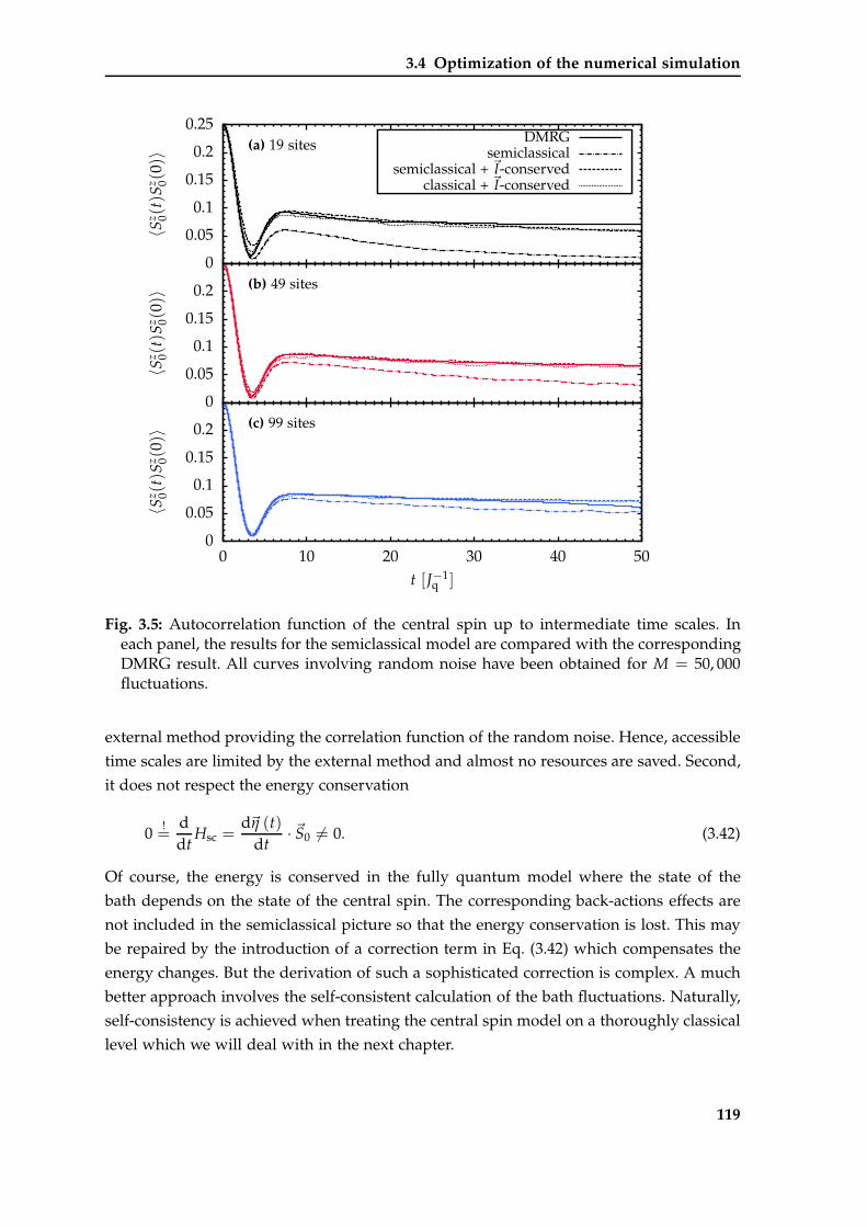
3.4 Optimization of the numerical simulation
0
0.05
0.1
0.15
0.2
0.25
〈Sz 0(
t)S
z 0(0)〉 (a) 19 sites
0
0.05
0.1
0.15
0.2
〈Sz 0(
t)S
z 0(0)〉 (b) 49 sites
0
0.05
0.1
0.15
0.2
0 10 20 30 40 50
〈Sz 0(
t)S
z 0(0)〉
t [J−1q ]
(c) 99 sites
DMRGsemiclassical
semiclassical + ~I-conservedclassical + ~I-conserved
Fig. 3.5: Autocorrelation function of the central spin up to intermediate time scales. Ineach panel, the results for the semiclassical model are compared with the correspondingDMRG result. All curves involving random noise have been obtained for M = 50, 000fluctuations.
external method providing the correlation function of the random noise. Hence, accessible
time scales are limited by the external method and almost no resources are saved. Second,
it does not respect the energy conservation
0 !=
ddt
Hsc =d~η (t)
dt· ~S0 6= 0. (3.42)
Of course, the energy is conserved in the fully quantum model where the state of the
bath depends on the state of the central spin. The corresponding back-actions effects are
not included in the semiclassical picture so that the energy conservation is lost. This may
be repaired by the introduction of a correction term in Eq. (3.42) which compensates the
energy changes. But the derivation of such a sophisticated correction is complex. A much
better approach involves the self-consistent calculation of the bath fluctuations. Naturally,
self-consistency is achieved when treating the central spin model on a thoroughly classical
level which we will deal with in the next chapter.
119
Chapter 3 Classical Gaussian Fluctuations in the Zero-Field Limit
3.5 Remarks on finite external magnetic fields
The discussion of the semiclassical model in the present chapter was restricted to the zero-
field limit where the model is completely isotropic. But the investigation may of course be
extended to finite external magnetic fields. For example, one can investigate the scenarios
discussed in Sect. 2.7.2 where the external magnetic field is applied either to the bath spins
or to the central spin.
In extension of the derivation of the AHT in the zero-field limit, we addressed the first
scenario where the field is applied to the bath spins. Then, the semiclassical Hamiltonian
remains unchanged but the random fluctuations ~η(t) obey a cylindric symmetry. We de-
rived the corresponding AHT up to second order. It requires the introduction of a cylindric
probability distribution which is renormalized similar to the second order in the zero-field
limit, see Appendix D. However, it turned out that the results only yield an insufficient ap-
proximation of the DMRG results. Hence, we refrain from presenting this treatment in the
present thesis because the unsatisfactory quality of the results does not justify the lengthy
derivation of the corresponding AHT. At first sight, the poor performance for the cylindric
symmetry might be surprising because the AHT worked well in the zero-field limit. Its
failure for finite external fields likely has to be attributed to the more complex correlations
of the random noise inducing anisotropic fluctuations as well as to cross-correlations. Fur-
thermore, the static character of the random fluctuations is much less pronounced because
the external fields induce a precession of the spins which is also reflected in the correlation
functions gαβ(t).
We also addressed finite external magnetic fields within the random noise simulation.
While the behavior in the spin directions perpendicular to the external field resembles the
behavior of the quantum model nicely, the plateau in the direction parallel to the external
field is not completely captured. Like in the zero-field limit, a significant decay is found
in the random noise simulation in contrast to the DMRG results. The optimized version of
the random noise simulation introduced in Sect. 3.4 may also be adapted to finite external
fields. Similarly to the zero-field limit, we suppose that the results should be significantly
improved. But the lack of energy conservation and the other disadvantages remain so that
we do not pursue this option further.
120
Chapter 4
Classical Equations of Motion
Contents
4.1 Introduction . . . . . . . . . . . . . . . . . . . . . . . . . . . . . . . . . . . . 122
4.2 Zero-field limit . . . . . . . . . . . . . . . . . . . . . . . . . . . . . . . . . . 124
4.3 Finite external magnetic field . . . . . . . . . . . . . . . . . . . . . . . . . 128
4.3.1 Weak-field regime . . . . . . . . . . . . . . . . . . . . . . . . . . . . 128
4.3.2 Intermediate-field regime . . . . . . . . . . . . . . . . . . . . . . . . 132
4.3.3 Strong-field regime . . . . . . . . . . . . . . . . . . . . . . . . . . . . 134
4.3.4 Summary . . . . . . . . . . . . . . . . . . . . . . . . . . . . . . . . . 137
The semiclassical model, which was introduced for an effective description of the central
spin dynamics in the last chapter, has proven to work quite well in the zero-field limit as
long as the bath size is not too small. However, the sampling of the random noise relies on
the correlation function of the Overhauser field which has to be known from an external
and independent source. Furthermore, the replacement of the quantum bath by a classical
random field does not respect the energy conservation. In this chapter, we circumvent
these problems by solving the complete set of classical equations of motion for the central
spin model. This approach implies a consistent calculation of the bath fluctuations. Hence,
no external method is required and a closed description of the classical spin dynamics for
both the central spin as well as for the bath spins is obtained.
After the brief introduction of the classical equations of motion in Sect. 4.1, their solutions
in presence and in absence of an external magnetic field are presented up to intermediate
time scales. The zero-field limit is addressed in Sect. 4.2, while the results for finite external
fields are discussed in Sect. 4.3. For the latter scenario, the external field is restricted
to the central spin for brevity and for experimental relevance. Precisely, we adopt the
scenarios from Sect. 2.7.2.2 where the weak, the intermediate, and the strong-field regime
was investigated by DMRG on short-time scales.
121
Chapter 4 Classical Equations of Motion
4.1 Introduction
Classically, the spin dynamics in the central spin model is determined by the 3(N + 1)
equations of motion (EOMs)
ddt
~S0 = ~A × ~S0 −~h0 × ~S0 (4.1a)
ddt
~Si = Ji~S0 × ~Si, (4.1b)
where i ∈ 1, 2, . . . , N and ~h0 is the external field applied to the central spin. As for the
quantum model, the classical Overhauser field is defined by
~A :=N
∑i=1
Ji~Si. (4.2)
Note, however, that the Overhauser field is now a simple vector in R3 and not an operator
anymore as in the quantum model. It is easily verified that the total energy
E = ~A · ~S0
⇒ dE
dt= ~A · ~S0 + ~A · ~S0 = 0
(4.3)
is conserved because of the properties of the outer product.
The set (4.1) of coupled EOMs is solved best using standard numerical routines such as
Runge-Kutta integration. Here, we stick to the adaptive Runge-Kutta-Fehlberg method
which is part of the GNU Scientific Library (GSL) [GDT+09]. The initial values for all
spins ~Si(t) at t = 0 are chosen from a random distribution with vanishing mean value and
variance
Sαi (0)S
αi (0) =
14
. (4.4)
By carrying out the numerical integration, one obtains all spins ~Si as function of time.
Thereby, the desired autocorrelation functions are calculated by averaging over a large
number M of random initial configurations. This corresponds to the investigation of a
completely unpolarized system. The conservation of the energy and of the total spin has
explicitly been checked to verify the correctness of the implementation. The energy in the
regarded time interval t ∈ [0, 1000 J−1q ] is conserved up to order 10−6 which also corre-
sponds to the step-size of the Runge-Kutta integration. On the same time scale, the total
momentum is conserved up to order 10−12. Decreasing the step-size of the Runge-Kutta
method did not lead to a significant improvement so that we use 10−6 as standard value.
122
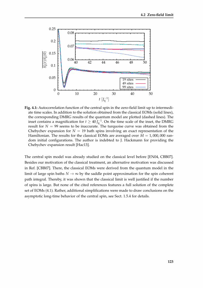
4.2 Zero-field limit
0
0.05
0.1
0.15
0.2
0.25
0 10 20 30 40 50
Sz 0(
t)S
z 0(0)
t [J−1q ]
0.06
0.07
0.08
40 42 44 46 48 50
19 sites49 sites99 sites
Fig. 4.1: Autocorrelation function of the central spin in the zero-field limit up to intermedi-ate time scales. In addition to the solution obtained from the classical EOMs (solid lines),the corresponding DMRG results of the quantum model are plotted (dashed lines). Theinset contains a magnification for t ≥ 40 J−1
q . On the time scale of the inset, the DMRGresult for N = 99 seems to be inaccurate. The turquoise curve was obtained from theChebychev expansion for N = 19 bath spins involving an exact representation of theHamiltonian. The results for the classical EOMs are averaged over M = 1, 000, 000 ran-dom initial configurations. The author is indebted to J. Hackmann for providing theChebychev expansion result [Hac13].
The central spin model was already studied on the classical level before [EN04, CBB07].
Besides our motivation of the classical treatment, an alternative motivation was discussed
in Ref. [CBB07]. There, the classical EOMs were derived from the quantum model in the
limit of large spin baths N → ∞ by the saddle point approximation for the spin coherent
path integral. Thereby, it was shown that the classical limit is well justified if the number
of spins is large. But none of the cited references features a full solution of the complete
set of EOMs (4.1). Rather, additional simplifications were made to draw conclusions on the
asymptotic long-time behavior of the central spin, see Sect. 1.5.4 for details.
123
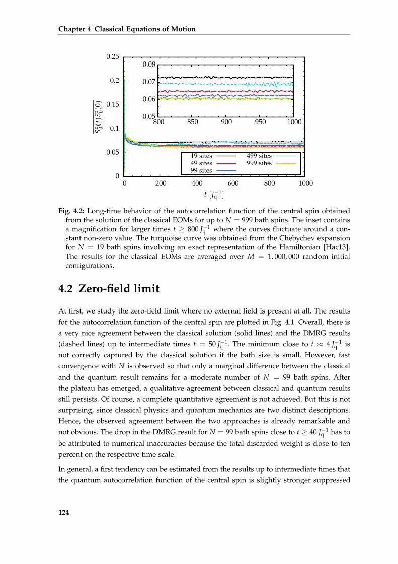
Chapter 4 Classical Equations of Motion
0
0.05
0.1
0.15
0.2
0.25
0 200 400 600 800 1000
Sz 0(
t)S
z 0(0)
t [J−1q ]
0.05
0.06
0.07
0.08
800 850 900 950 1000
19 sites49 sites99 sites
499 sites999 sites
Fig. 4.2: Long-time behavior of the autocorrelation function of the central spin obtainedfrom the solution of the classical EOMs for up to N = 999 bath spins. The inset containsa magnification for larger times t ≥ 800 J−1
q where the curves fluctuate around a con-stant non-zero value. The turquoise curve was obtained from the Chebychev expansionfor N = 19 bath spins involving an exact representation of the Hamiltonian [Hac13].The results for the classical EOMs are averaged over M = 1, 000, 000 random initialconfigurations.
4.2 Zero-field limit
At first, we study the zero-field limit where no external field is present at all. The results
for the autocorrelation function of the central spin are plotted in Fig. 4.1. Overall, there is
a very nice agreement between the classical solution (solid lines) and the DMRG results
(dashed lines) up to intermediate times t = 50 J−1q . The minimum close to t ≈ 4 J−1
q is
not correctly captured by the classical solution if the bath size is small. However, fast
convergence with N is observed so that only a marginal difference between the classical
and the quantum result remains for a moderate number of N = 99 bath spins. After
the plateau has emerged, a qualitative agreement between classical and quantum results
still persists. Of course, a complete quantitative agreement is not achieved. But this is not
surprising, since classical physics and quantum mechanics are two distinct descriptions.
Hence, the observed agreement between the two approaches is already remarkable and
not obvious. The drop in the DMRG result for N = 99 bath spins close to t ≥ 40 J−1q has to
be attributed to numerical inaccuracies because the total discarded weight is close to ten
percent on the respective time scale.
In general, a first tendency can be estimated from the results up to intermediate times that
the quantum autocorrelation function of the central spin is slightly stronger suppressed
124
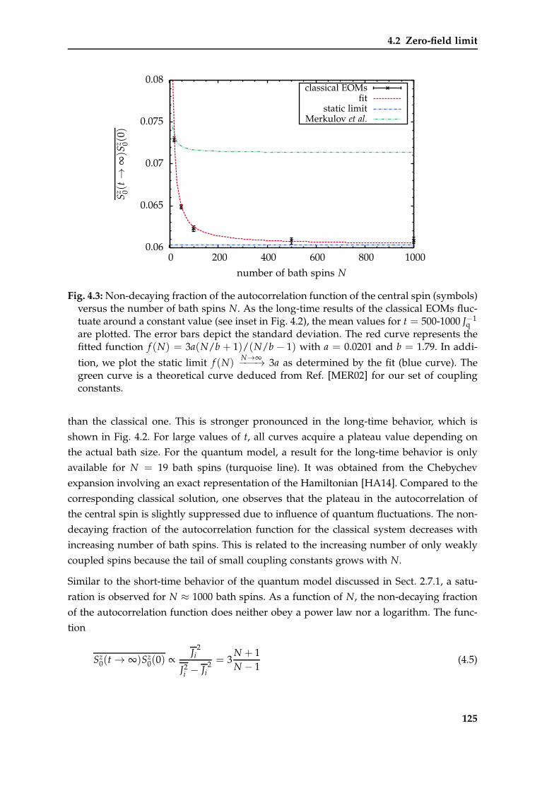
4.2 Zero-field limit
0.06
0.065
0.07
0.075
0.08
0 200 400 600 800 1000
Sz 0(
t→
∞)S
z 0(0)
number of bath spins N
classical EOMsfit
static limitMerkulov et al.
Fig. 4.3: Non-decaying fraction of the autocorrelation function of the central spin (symbols)versus the number of bath spins N. As the long-time results of the classical EOMs fluc-tuate around a constant value (see inset in Fig. 4.2), the mean values for t = 500-1000 J−1
qare plotted. The error bars depict the standard deviation. The red curve represents thefitted function f (N) = 3a(N/b + 1)/(N/b − 1) with a = 0.0201 and b = 1.79. In addi-
tion, we plot the static limit f (N)N→∞−−−→ 3a as determined by the fit (blue curve). The
green curve is a theoretical curve deduced from Ref. [MER02] for our set of couplingconstants.
than the classical one. This is stronger pronounced in the long-time behavior, which is
shown in Fig. 4.2. For large values of t, all curves acquire a plateau value depending on
the actual bath size. For the quantum model, a result for the long-time behavior is only
available for N = 19 bath spins (turquoise line). It was obtained from the Chebychev
expansion involving an exact representation of the Hamiltonian [HA14]. Compared to the
corresponding classical solution, one observes that the plateau in the autocorrelation of
the central spin is slightly suppressed due to influence of quantum fluctuations. The non-
decaying fraction of the autocorrelation function for the classical system decreases with
increasing number of bath spins. This is related to the increasing number of only weakly
coupled spins because the tail of small coupling constants grows with N.
Similar to the short-time behavior of the quantum model discussed in Sect. 2.7.1, a satu-
ration is observed for N ≈ 1000 bath spins. As a function of N, the non-decaying fraction
of the autocorrelation function does neither obey a power law nor a logarithm. The func-
tion
Sz0(t → ∞)Sz
0(0) ∝Ji
2
J2i − Ji
2 = 3N + 1N − 1
(4.5)
125
Chapter 4 Classical Equations of Motion
provides a good fit to the numerical data if the prefactor and the bath size N are appro-
priately renormalized, see Fig. 4.3. Thereby, one deduces that the autocorrelation function
of the central spin never exhibits a complete decay. A certain fraction always persists even
in the asymptotic limit N → ∞. From the fit to our numerical data for the classical set of
EOMs, one deduces that Sz0(∞)Sz
0(0) ≈ 0.06 for N → ∞, see caption of Fig. 4.3. However,
we cannot provide an analytical argument for the observed behavior as a function of N.
In Ref. [MER02], an estimate for the non-decaying fraction was derived by including the
fluctuations of the nuclear bath. Compared to the full solution of the classical EOMs, the
integrals derived by Merkulov et al. overestimate the non-decaying fraction. Overall, the
asymptotic value deduced from their theory for our parameters is roughly 20 % larger than
the numerical solution of the classical EOMs, see Fig. 4.3. Note, however, that the quantity
Ji2/(J2
i − Ji2) enters in their calculations.
In total, the dynamics of the electron spin in the zero-field limit is essentially classical up
to intermediate time scales. On the long-time scale, the influence of quantum fluctuations
increases which is expressed by a reduced non-decaying fraction of the autocorrelation
function of the quantum model. Although the reduction in the inset in Fig. 4.2 is rather
small and almost of the order of the error due to averaging over a finite number of random
initial configurations, it has to be regarded as significant. But the results for t ≤ 50 J−1q sug-
gest that the differences between the classical and the quantum description will dissolve if
N is large. In essence, our observations agree with results by Coish et al. [CLYA07]. They
compared the quantum solution with the corresponding classical solution for a single ini-
tial state and found that the dynamics is essentially classical up to a certain time. Beyond
that time, quantum fluctuations have to be taken into account. However, they did not study
the average over all initial conditions as we do. Furthermore, all couplings in their study
were homogeneous Ji = J and the expectation values of the observables were calculated
on the mean-field level. A numerical solution of the full set of EOMs was not considered.
Furthermore, our result for the isotropic model seems to resemble the one presented in
Ref. [AHDDH06], despite the different distribution of the coupling constants. The method
in Ref. [AHDDH06] also involves a classical treatment of the central spin dynamics in
the unpolarized model. It is derived from the P-representation of the central spin density
matrix. The authors claim to reproduce the exact EOMs for the part describing the central
spin, while the behavior of the bath seems not to be captured correctly. The derivation
of the EOMs in Ref. [AHDDH06] is kept very short and remains rather elusive so that a
classification of the approach compared the classical EOMs given in Eq. (4.1) is difficult.
It is a very interesting feature that, even for large times t > 100 J−1q , the results converge
already for N ≈ 1000 bath spins. In a real quantum dot, the number of bath spins is
roughly one to two orders of magnitude larger, see Sect. 1.3. Hence, one may assume that
126
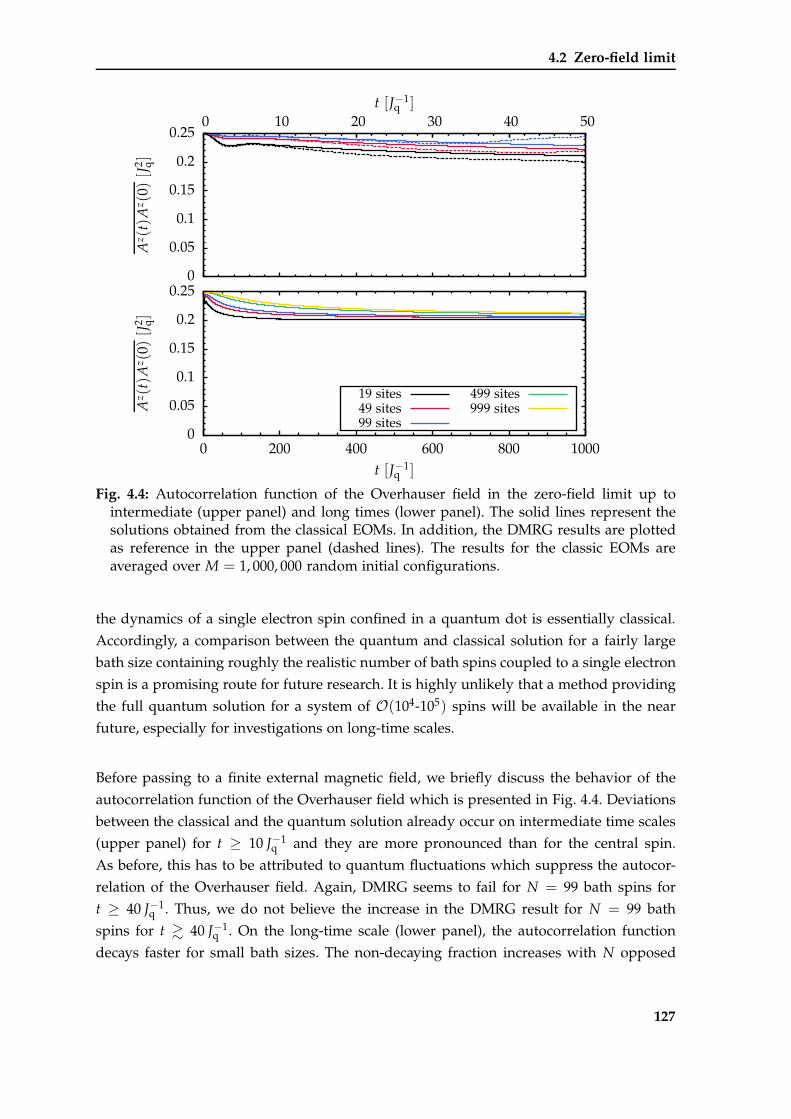
4.2 Zero-field limit
0
0.05
0.1
0.15
0.2
0.250 10 20 30 40 50
Az(t)A
z(0)[J
2 q]
t [J−1q ]
0
0.05
0.1
0.15
0.2
0.25
0 200 400 600 800 1000
Az(t)A
z(0)[J
2 q]
t [J−1q ]
19 sites49 sites99 sites
499 sites999 sites
Fig. 4.4: Autocorrelation function of the Overhauser field in the zero-field limit up tointermediate (upper panel) and long times (lower panel). The solid lines represent thesolutions obtained from the classical EOMs. In addition, the DMRG results are plottedas reference in the upper panel (dashed lines). The results for the classic EOMs areaveraged over M = 1, 000, 000 random initial configurations.
the dynamics of a single electron spin confined in a quantum dot is essentially classical.
Accordingly, a comparison between the quantum and classical solution for a fairly large
bath size containing roughly the realistic number of bath spins coupled to a single electron
spin is a promising route for future research. It is highly unlikely that a method providing
the full quantum solution for a system of O(104-105) spins will be available in the near
future, especially for investigations on long-time scales.
Before passing to a finite external magnetic field, we briefly discuss the behavior of the
autocorrelation function of the Overhauser field which is presented in Fig. 4.4. Deviations
between the classical and the quantum solution already occur on intermediate time scales
(upper panel) for t ≥ 10 J−1q and they are more pronounced than for the central spin.
As before, this has to be attributed to quantum fluctuations which suppress the autocor-
relation of the Overhauser field. Again, DMRG seems to fail for N = 99 bath spins for
t ≥ 40 J−1q . Thus, we do not believe the increase in the DMRG result for N = 99 bath
spins for t & 40 J−1q . On the long-time scale (lower panel), the autocorrelation function
decays faster for small bath sizes. The non-decaying fraction increases with N opposed
127
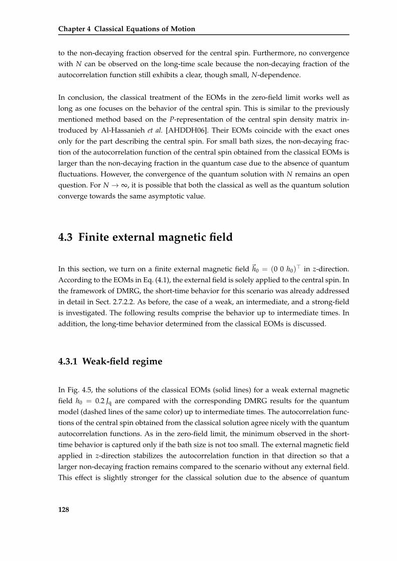
Chapter 4 Classical Equations of Motion
to the non-decaying fraction observed for the central spin. Furthermore, no convergence
with N can be observed on the long-time scale because the non-decaying fraction of the
autocorrelation function still exhibits a clear, though small, N-dependence.
In conclusion, the classical treatment of the EOMs in the zero-field limit works well as
long as one focuses on the behavior of the central spin. This is similar to the previously
mentioned method based on the P-representation of the central spin density matrix in-
troduced by Al-Hassanieh et al. [AHDDH06]. Their EOMs coincide with the exact ones
only for the part describing the central spin. For small bath sizes, the non-decaying frac-
tion of the autocorrelation function of the central spin obtained from the classical EOMs is
larger than the non-decaying fraction in the quantum case due to the absence of quantum
fluctuations. However, the convergence of the quantum solution with N remains an open
question. For N → ∞, it is possible that both the classical as well as the quantum solution
converge towards the same asymptotic value.
4.3 Finite external magnetic field
In this section, we turn on a finite external magnetic field ~h0 = (0 0 h0)⊤ in z-direction.
According to the EOMs in Eq. (4.1), the external field is solely applied to the central spin. In
the framework of DMRG, the short-time behavior for this scenario was already addressed
in detail in Sect. 2.7.2.2. As before, the case of a weak, an intermediate, and a strong-field
is investigated. The following results comprise the behavior up to intermediate times. In
addition, the long-time behavior determined from the classical EOMs is discussed.
4.3.1 Weak-field regime
In Fig. 4.5, the solutions of the classical EOMs (solid lines) for a weak external magnetic
field h0 = 0.2 Jq are compared with the corresponding DMRG results for the quantum
model (dashed lines of the same color) up to intermediate times. The autocorrelation func-
tions of the central spin obtained from the classical solution agree nicely with the quantum
autocorrelation functions. As in the zero-field limit, the minimum observed in the short-
time behavior is captured only if the bath size is not too small. The external magnetic field
applied in z-direction stabilizes the autocorrelation function in that direction so that a
larger non-decaying fraction remains compared to the scenario without any external field.
This effect is slightly stronger for the classical solution due to the absence of quantum
128
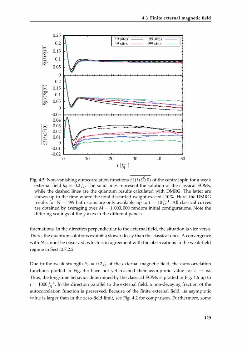
4.3 Finite external magnetic field
0
0.05
0.1
0.15
0.2
0.25
Sz 0(
t)S
z 0(0)
-0.050
0.050.1
0.150.2
Sx 0(t)S
x 0(0)
-0.02-0.01
00.010.020.030.04
0 10 20 30 40 50
Sx 0(t)S
y 0(0)
t [J−1q ]
19 sites49 sites
99 sites499 sites
Fig. 4.5: Non-vanishing autocorrelation functions Sα0(t)S
β0 (0) of the central spin for a weak
external field h0 = 0.2 Jq. The solid lines represent the solution of the classical EOMs,while the dashed lines are the quantum results calculated with DMRG. The latter areshown up to the time where the total discarded weight exceeds 10 %. Here, the DMRGresults for N = 499 bath spins are only available up to t = 10 J−1
q . All classical curvesare obtained by averaging over M = 1, 000, 000 random initial configurations. Note thediffering scalings of the y-axes in the different panels.
fluctuations. In the direction perpendicular to the external field, the situation is vice versa.
There, the quantum solutions exhibit a slower decay than the classical ones. A convergence
with N cannot be observed, which is in agreement with the observations in the weak-field
regime in Sect. 2.7.2.2.
Due to the weak strength h0 = 0.2 Jq of the external magnetic field, the autocorrelation
functions plotted in Fig. 4.5 have not yet reached their asymptotic value for t → ∞.
Thus, the long-time behavior determined by the classical EOMs is plotted in Fig. 4.6 up to
t = 1000 J−1q . In the direction parallel to the external field, a non-decaying fraction of the
autocorrelation function is preserved. Because of the finite external field, its asymptotic
value is larger than in the zero-field limit, see Fig. 4.2 for comparison. Furthermore, some
129
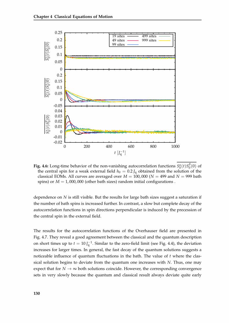
Chapter 4 Classical Equations of Motion
0
0.05
0.1
0.15
0.2
0.25
Sz 0(
t)S
z 0(0)
-0.050
0.050.1
0.150.2
Sx 0(t)S
x 0(0)
-0.02-0.01
00.010.020.030.04
0 200 400 600 800 1000
Sx 0(t)S
y 0(0)
t [J−1q ]
19 sites49 sites99 sites
499 sites999 sites
Fig. 4.6: Long-time behavior of the non-vanishing autocorrelation functions Sα0(t)S
β0 (0) of
the central spin for a weak external field h0 = 0.2 Jq obtained from the solution of theclassical EOMs. All curves are averaged over M = 100, 000 (N = 499 and N = 999 bathspins) or M = 1, 000, 000 (other bath sizes) random initial configurations .
dependence on N is still visible. But the results for large bath sizes suggest a saturation if
the number of bath spins is increased further. In contrast, a slow but complete decay of the
autocorrelation functions in spin directions perpendicular is induced by the precession of
the central spin in the external field.
The results for the autocorrelation functions of the Overhauser field are presented in
Fig. 4.7. They reveal a good agreement between the classical and the quantum description
on short times up to t = 10 J−1q . Similar to the zero-field limit (see Fig. 4.4), the deviation
increases for larger times. In general, the fast decay of the quantum solutions suggests a
noticeable influence of quantum fluctuations in the bath. The value of t where the clas-
sical solution begins to deviate from the quantum one increases with N. Thus, one may
expect that for N → ∞ both solutions coincide. However, the corresponding convergence
sets in very slowly because the quantum and classical result always deviate quite early
130
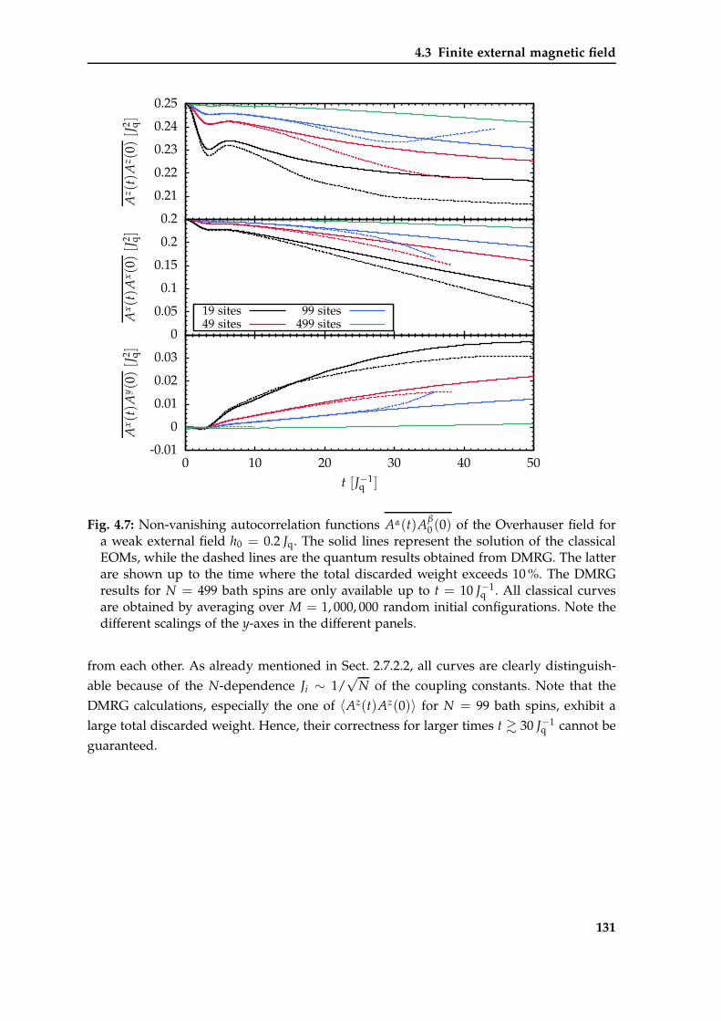
4.3 Finite external magnetic field
0.2
0.21
0.22
0.23
0.24
0.25
Az(t)A
z(0)[J
2 q]
0
0.05
0.1
0.15
0.2
Ax(t)A
x(0)[J
2 q]
-0.01
0
0.01
0.02
0.03
0 10 20 30 40 50
Ax(t)A
y(0)[J
2 q]
t [J−1q ]
19 sites49 sites
99 sites499 sites
Fig. 4.7: Non-vanishing autocorrelation functions Aα(t)Aβ0 (0) of the Overhauser field for
a weak external field h0 = 0.2 Jq. The solid lines represent the solution of the classicalEOMs, while the dashed lines are the quantum results obtained from DMRG. The latterare shown up to the time where the total discarded weight exceeds 10 %. The DMRGresults for N = 499 bath spins are only available up to t = 10 J−1
q . All classical curvesare obtained by averaging over M = 1, 000, 000 random initial configurations. Note thedifferent scalings of the y-axes in the different panels.
from each other. As already mentioned in Sect. 2.7.2.2, all curves are clearly distinguish-
able because of the N-dependence Ji ∼ 1/√
N of the coupling constants. Note that the
DMRG calculations, especially the one of 〈Az(t)Az(0)〉 for N = 99 bath spins, exhibit a
large total discarded weight. Hence, their correctness for larger times t & 30 J−1q cannot be
guaranteed.
131
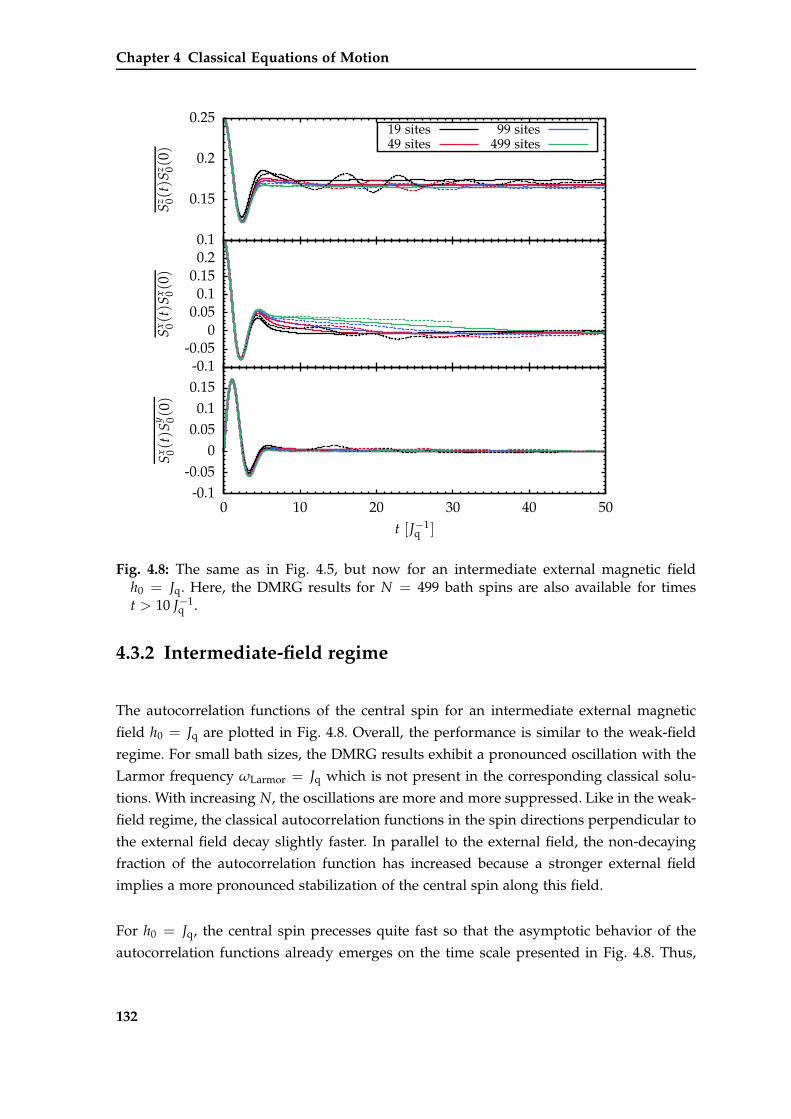
Chapter 4 Classical Equations of Motion
0.1
0.15
0.2
0.25
Sz 0(
t)S
z 0(0)
-0.1-0.05
00.050.1
0.150.2
Sx 0(t)S
x 0(0)
-0.1-0.05
00.050.1
0.15
0 10 20 30 40 50
Sx 0(t)S
y 0(0)
t [J−1q ]
19 sites49 sites
99 sites499 sites
Fig. 4.8: The same as in Fig. 4.5, but now for an intermediate external magnetic fieldh0 = Jq. Here, the DMRG results for N = 499 bath spins are also available for timest > 10 J−1
q .
4.3.2 Intermediate-field regime
The autocorrelation functions of the central spin for an intermediate external magnetic
field h0 = Jq are plotted in Fig. 4.8. Overall, the performance is similar to the weak-field
regime. For small bath sizes, the DMRG results exhibit a pronounced oscillation with the
Larmor frequency ωLarmor = Jq which is not present in the corresponding classical solu-
tions. With increasing N, the oscillations are more and more suppressed. Like in the weak-
field regime, the classical autocorrelation functions in the spin directions perpendicular to
the external field decay slightly faster. In parallel to the external field, the non-decaying
fraction of the autocorrelation function has increased because a stronger external field
implies a more pronounced stabilization of the central spin along this field.
For h0 = Jq, the central spin precesses quite fast so that the asymptotic behavior of the
autocorrelation functions already emerges on the time scale presented in Fig. 4.8. Thus,
132
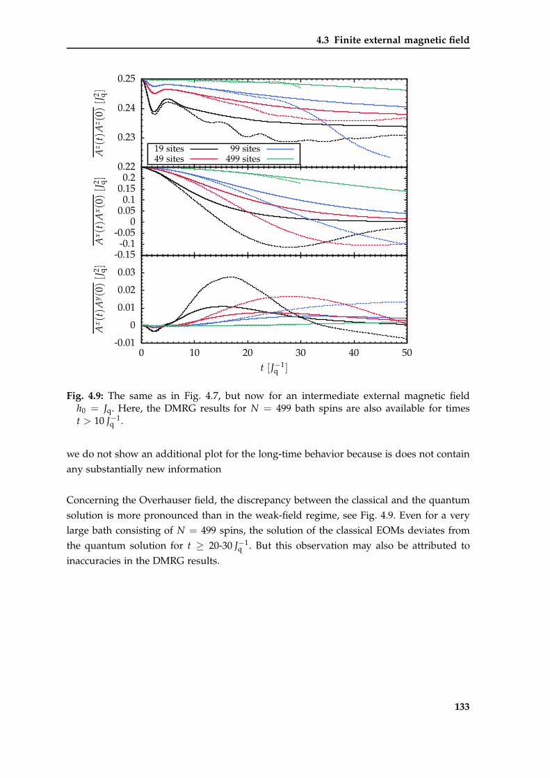
4.3 Finite external magnetic field
0.22
0.23
0.24
0.25
Az(t)A
z(0)[J
2 q]
-0.15-0.1
-0.050
0.050.1
0.150.2
Ax(t)A
x(0)[J
2 q]
-0.01
0
0.01
0.02
0.03
0 10 20 30 40 50
Ax(t)A
y(0)[J
2 q]
t [J−1q ]
19 sites49 sites
99 sites499 sites
Fig. 4.9: The same as in Fig. 4.7, but now for an intermediate external magnetic fieldh0 = Jq. Here, the DMRG results for N = 499 bath spins are also available for timest > 10 J−1
q .
we do not show an additional plot for the long-time behavior because is does not contain
any substantially new information
Concerning the Overhauser field, the discrepancy between the classical and the quantum
solution is more pronounced than in the weak-field regime, see Fig. 4.9. Even for a very
large bath consisting of N = 499 spins, the solution of the classical EOMs deviates from
the quantum solution for t ≥ 20-30 J−1q . But this observation may also be attributed to
inaccuracies in the DMRG results.
133
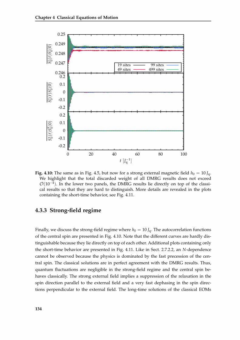
Chapter 4 Classical Equations of Motion
0.246
0.247
0.248
0.249
0.25
Sz 0(
t)S
z 0(0)
-0.2
-0.1
0
0.1
0.2
Sx 0(t)S
x 0(0)
-0.2
-0.1
0
0.1
0.2
0 20 40 60 80 100
Sx 0(t)S
y 0(0)
t [J−1q ]
19 sites49 sites
99 sites499 sites
Fig. 4.10: The same as in Fig. 4.5, but now for a strong external magnetic field h0 = 10 Jq.We highlight that the total discarded weight of all DMRG results does not exceedO(10−4). In the lower two panels, the DMRG results lie directly on top of the classi-cal results so that they are hard to distinguish. More details are revealed in the plotscontaining the short-time behavior, see Fig. 4.11.
4.3.3 Strong-field regime
Finally, we discuss the strong-field regime where h0 = 10 Jq. The autocorrelation functions
of the central spin are presented in Fig. 4.10. Note that the different curves are hardly dis-
tinguishable because they lie directly on top of each other. Additional plots containing only
the short-time behavior are presented in Fig. 4.11. Like in Sect. 2.7.2.2, an N-dependence
cannot be observed because the physics is dominated by the fast precession of the cen-
tral spin. The classical solutions are in perfect agreement with the DMRG results. Thus,
quantum fluctuations are negligible in the strong-field regime and the central spin be-
haves classically. The strong external field implies a suppression of the relaxation in the
spin direction parallel to the external field and a very fast dephasing in the spin direc-
tions perpendicular to the external field. The long-time solutions of the classical EOMs
134
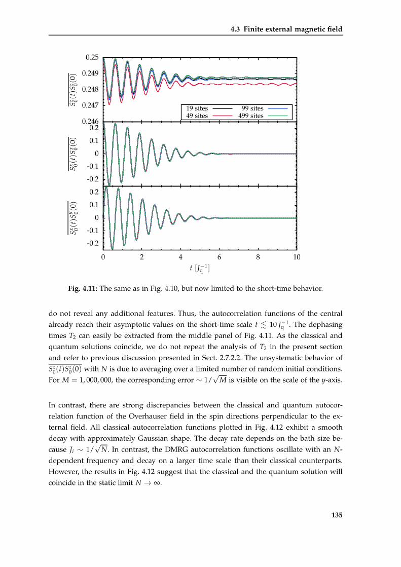
4.3 Finite external magnetic field
0.246
0.247
0.248
0.249
0.25
Sz 0(
t)S
z 0(0)
-0.2
-0.1
0
0.1
0.2
Sx 0(t)S
x 0(0)
-0.2
-0.1
0
0.1
0.2
0 2 4 6 8 10
Sx 0(t)S
y 0(0)
t [J−1q ]
19 sites49 sites
99 sites499 sites
Fig. 4.11: The same as in Fig. 4.10, but now limited to the short-time behavior.
do not reveal any additional features. Thus, the autocorrelation functions of the central
already reach their asymptotic values on the short-time scale t . 10 J−1q . The dephasing
times T2 can easily be extracted from the middle panel of Fig. 4.11. As the classical and
quantum solutions coincide, we do not repeat the analysis of T2 in the present section
and refer to previous discussion presented in Sect. 2.7.2.2. The unsystematic behavior of
Sz0(t)S
z0(0) with N is due to averaging over a limited number of random initial conditions.
For M = 1, 000, 000, the corresponding error ∼ 1/√
M is visible on the scale of the y-axis.
In contrast, there are strong discrepancies between the classical and quantum autocor-
relation function of the Overhauser field in the spin directions perpendicular to the ex-
ternal field. All classical autocorrelation functions plotted in Fig. 4.12 exhibit a smooth
decay with approximately Gaussian shape. The decay rate depends on the bath size be-
cause Ji ∼ 1/√
N. In contrast, the DMRG autocorrelation functions oscillate with an N-
dependent frequency and decay on a larger time scale than their classical counterparts.
However, the results in Fig. 4.12 suggest that the classical and the quantum solution will
coincide in the static limit N → ∞.
135
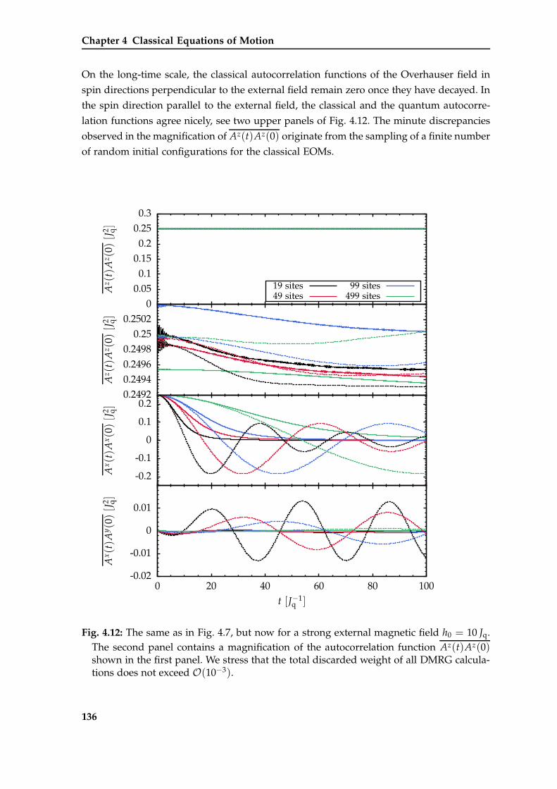
Chapter 4 Classical Equations of Motion
On the long-time scale, the classical autocorrelation functions of the Overhauser field in
spin directions perpendicular to the external field remain zero once they have decayed. In
the spin direction parallel to the external field, the classical and the quantum autocorre-
lation functions agree nicely, see two upper panels of Fig. 4.12. The minute discrepancies
observed in the magnification of Az(t)Az(0) originate from the sampling of a finite number
of random initial configurations for the classical EOMs.
00.050.1
0.150.2
0.250.3
Az(t)A
z(0)[J
2 q]
0.24920.24940.24960.2498
0.250.2502
Az(t)A
z(0)[J
2 q]
-0.2
-0.1
0
0.1
0.2
Ax(t)A
x(0)[J
2 q]
-0.02
-0.01
0
0.01
0 20 40 60 80 100
Ax(t)A
y(0)[J
2 q]
t [J−1q ]
19 sites49 sites
99 sites499 sites
Fig. 4.12: The same as in Fig. 4.7, but now for a strong external magnetic field h0 = 10 Jq.The second panel contains a magnification of the autocorrelation function Az(t)Az(0)shown in the first panel. We stress that the total discarded weight of all DMRG calcula-tions does not exceed O(10−3).
136
4.3 Finite external magnetic field
4.3.4 Summary
In total, the performance of the classical spin dynamics in a finite external magnetic field
h0 is similar to the zero-field limit. The essential dynamics of the central spin is well cap-
tured by the classical EOMs. For weak and intermediate values of h0, a noticeable influence
of quantum fluctuations still persists on intermediate time scales leading to a quantitative
deviation between the classical and the DMRG result. Still, for large baths one observes
qualitatively the same behavior. In the spin direction parallel to the external field, quan-
tum fluctuations induce a marginal reduction of the autocorrelation function. Perpendic-
ular to h0, the classical autocorrelation functions decay slightly faster than their quantum
counterparts. For a very strong external field, the quantum and classical solutions cannot
be distinguished. In this regime, the dependence on the number N of bath spins is also
gone. Generally, the classical EOMs capture the crossover from the weak to the strong-
field regime as described in Sect. 2.7.2.2 and in Ref. [ZDAH+06]. Note that DMRG also
exhibits a very good performance in the strong-field regime, see Sect. 2.7.2.2. The external
field suppresses the relaxation of the central spin. Hence, the number of important states
increases significantly slower with t implying a reduction of the total discarded weight. In
consequence, the code runs faster and much larger times can be reached. This fact is also
expressed by the small total discarded weight. Even on long time scales, it does not exceed
O(10−4-10−3) in all DMRG calculations.
However, the classical treatment of the Overhauser field is not very successful. This effect
is more pronounced for a strong external field than for a weak field. Due to the fast preces-
sion of the central spin in the external field, the classical bath spins feel only an effective
average field of the central spin. This induces the smooth decay of the corresponding au-
tocorrelation functions and suppresses the oscillations in the Overhauser field. As long
as the field is rather weak and the bath contains a sufficiently large number of spins, the
classical solution yields a relatively good approximation to the quantum solution up to
limited values of t. For larger times, the behavior of a finite-size quantum bath will always
differ from the corresponding classical bath.
137

Chapter 5
Pulses for Pure Dephasing
Contents
5.1 Semiclassical model for pure dephasing . . . . . . . . . . . . . . . . . . . 140
5.2 Frobenius norm . . . . . . . . . . . . . . . . . . . . . . . . . . . . . . . . . . 141
5.3 Simulation of pulses . . . . . . . . . . . . . . . . . . . . . . . . . . . . . . . 142
5.4 Average Hamiltonian theory . . . . . . . . . . . . . . . . . . . . . . . . . . 147
5.4.1 Analytical expression for the Frobenius norm . . . . . . . . . . . . 147
5.4.2 Magnus expansion . . . . . . . . . . . . . . . . . . . . . . . . . . . . 148
5.4.3 Unexpected contributions for autocorrelation functions displayinga cusp at t = 0 . . . . . . . . . . . . . . . . . . . . . . . . . . . . . . 150
5.4.4 Verification for the CORPSE and SCORPSE pulse . . . . . . . . . . 153
In this chapter, we discuss a semiclassical model to study the fidelity of shaped π-pulses.
The semiclassical approach to the central spin problem is well-known from Chapter 3.
As already mentioned in Sect. 1.6 of the Introduction, real pulses with finite amplitude
and duration can be optimized by shaping their amplitudes and switching instances. This
makes them closer to an ideal pulse leading to a substantial increase of their performance
compared to an unshaped pulse of finite length.
At first, a semiclassical model for simulating optimized pulses suppressing the dephasing
of an electron spin is introduced in Sect. 5.1. For the numerical investigation of shaped
pulses, it is essential to quantify their fidelity. An appropriate measure for the deviation
of a shaped pulse from an ideal one is introduced in Sect. 5.2. The numerical results pre-
sented in Sect. 5.3 reveal an unexpected behavior of the pulses when the autocorrelation
function has a cusp at t = 0. This can be explained on the level of average Hamiltonian
theory, which is derived and verified in Sect. 5.4. Furthermore, we specify the supplemen-
tal condition which may be incorporated in the design of optimized pulses in addition to
the well-known standard conditions for a first order pulse. In Appendix G, it is proven
139
Chapter 5 Pulses for Pure Dephasing
that a simultaneous fulfillment of all conditions is excluded rigorously. Hence, only a min-
imization of the supplemental condition can be achieved when the standard first order
conditions are fulfilled.
5.1 Semiclassical model for pure dephasing
The upcoming discussion is restricted to pulses comprising solely the dephasing of the
electron spin. Dephasing is the primary contribution to the decoherence of an electron
spin in a quantum dot because experiments revealed that the longitudinal relaxation takes
place on a much larger time scale T1 ≫ T2, see Sect. 1.3. Thus, we may study a simplified
semiclassical model
Htot(t) = H(t) + Hp(t)
= η (t) σz + v (t) σx,(5.1)
where σα are the Pauli matrices. For simplicity, the factor 1/2 of the spin operators has
been neglected. The control Hamiltonian
Hp (t) = v (t) σx (5.2a)
describes a pulse of amplitude v(t) rotating the electron spin around the x-axis. The bath
is represented by a single random field η(t) obeying Gaussian statistics. It couples to the
electron spin in z-direction
H (t) = η (t) σz. (5.2b)
As introduced in Chapter 3, the Gaussian fluctuations are fully described by their auto-
correlation function g(t) = η(t)η(0) and their mean value η(t) = 0. As before, the latter
is again set to zero. In the semiclassical model (5.1), the energy scale is determined by
the parameter g0. It enters in the initial value g(0) = g20 of the correlation function of the
random noise and characterizes the amplitude of the fluctuations η(t).
A semiclassical model such as (5.1) has already been frequently used for the simulation of
pulses and pulse sequences with different backgrounds and for various types of Gaussian
and non-Gaussian noise [MdSZW06, CLNDS08, KMB+08, dLWR+10, BB11]. Compared to
a purely quantum mechanical model, only a moderate amount of CPU time is required
for the numerical investigation. Furthermore, pulses optimized specifically for a classical
bath [SFPU12, Sti12] can be simulated. Pulses shaped for a quantum bath may be studied
as well because they have to fulfill additional conditions compared to pulses derived for a
classical bath.
140
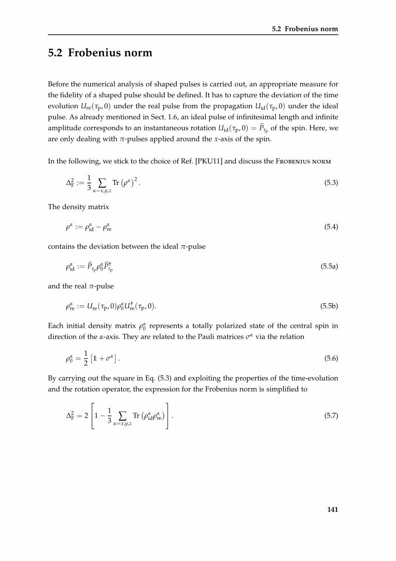
5.2 Frobenius norm
5.2 Frobenius norm
Before the numerical analysis of shaped pulses is carried out, an appropriate measure for
the fidelity of a shaped pulse should be defined. It has to capture the deviation of the time
evolution Ure(τp, 0) under the real pulse from the propagation Uid(τp, 0) under the ideal
pulse. As already mentioned in Sect. 1.6, an ideal pulse of infinitesimal length and infinite
amplitude corresponds to an instantaneous rotation Uid(τp, 0) = Pτp of the spin. Here, we
are only dealing with π-pulses applied around the x-axis of the spin.
In the following, we stick to the choice of Ref. [PKU11] and discuss the Frobenius norm
∆2F :=
13 ∑
α=x,y,zTr(ρα)2 . (5.3)
The density matrix
ρα := ραid − ρα
re (5.4)
contains the deviation between the ideal π-pulse
ραid := Pτp
ρα0 P†
τp(5.5a)
and the real π-pulse
ραre := Ure(τp, 0)ρα
0U†re(τp, 0). (5.5b)
Each initial density matrix ρα0 represents a totally polarized state of the central spin in
direction of the α-axis. They are related to the Pauli matrices σα via the relation
ρα0 =
12
[1+ σα
]. (5.6)
By carrying out the square in Eq. (5.3) and exploiting the properties of the time-evolution
and the rotation operator, the expression for the Frobenius norm is simplified to
∆2F = 2
1 − 1
3 ∑α=x,y,z
Tr(ρα
idραre) . (5.7)
141
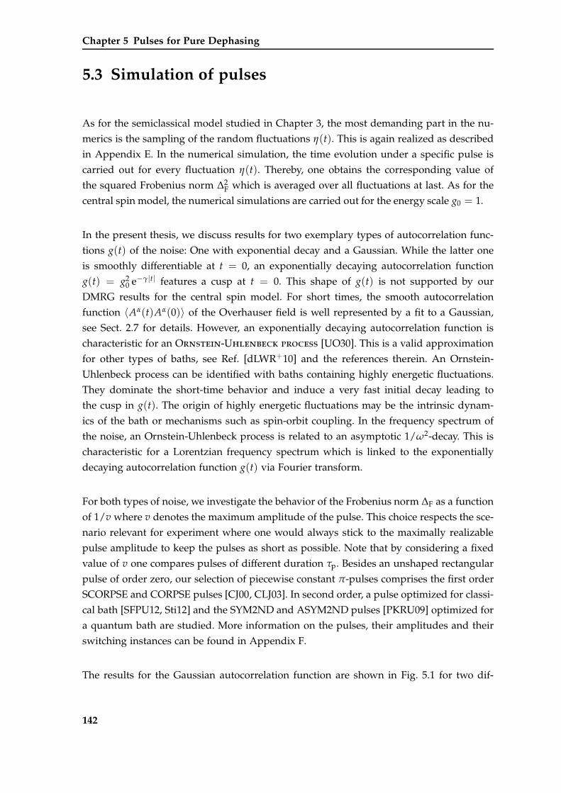
Chapter 5 Pulses for Pure Dephasing
5.3 Simulation of pulses
As for the semiclassical model studied in Chapter 3, the most demanding part in the nu-
merics is the sampling of the random fluctuations η(t). This is again realized as described
in Appendix E. In the numerical simulation, the time evolution under a specific pulse is
carried out for every fluctuation η(t). Thereby, one obtains the corresponding value of
the squared Frobenius norm ∆2F which is averaged over all fluctuations at last. As for the
central spin model, the numerical simulations are carried out for the energy scale g0 = 1.
In the present thesis, we discuss results for two exemplary types of autocorrelation func-
tions g(t) of the noise: One with exponential decay and a Gaussian. While the latter one
is smoothly differentiable at t = 0, an exponentially decaying autocorrelation function
g(t) = g20 e−γ|t| features a cusp at t = 0. This shape of g(t) is not supported by our
DMRG results for the central spin model. For short times, the smooth autocorrelation
function 〈Aα(t)Aα(0)〉 of the Overhauser field is well represented by a fit to a Gaussian,
see Sect. 2.7 for details. However, an exponentially decaying autocorrelation function is
characteristic for an Ornstein-Uhlenbeck process [UO30]. This is a valid approximation
for other types of baths, see Ref. [dLWR+10] and the references therein. An Ornstein-
Uhlenbeck process can be identified with baths containing highly energetic fluctuations.
They dominate the short-time behavior and induce a very fast initial decay leading to
the cusp in g(t). The origin of highly energetic fluctuations may be the intrinsic dynam-
ics of the bath or mechanisms such as spin-orbit coupling. In the frequency spectrum of
the noise, an Ornstein-Uhlenbeck process is related to an asymptotic 1/ω2-decay. This is
characteristic for a Lorentzian frequency spectrum which is linked to the exponentially
decaying autocorrelation function g(t) via Fourier transform.
For both types of noise, we investigate the behavior of the Frobenius norm ∆F as a function
of 1/v where v denotes the maximum amplitude of the pulse. This choice respects the sce-
nario relevant for experiment where one would always stick to the maximally realizable
pulse amplitude to keep the pulses as short as possible. Note that by considering a fixed
value of v one compares pulses of different duration τp. Besides an unshaped rectangular
pulse of order zero, our selection of piecewise constant π-pulses comprises the first order
SCORPSE and CORPSE pulses [CJ00, CLJ03]. In second order, a pulse optimized for classi-
cal bath [SFPU12, Sti12] and the SYM2ND and ASYM2ND pulses [PKRU09] optimized for
a quantum bath are studied. More information on the pulses, their amplitudes and their
switching instances can be found in Appendix F.
The results for the Gaussian autocorrelation function are shown in Fig. 5.1 for two dif-
142
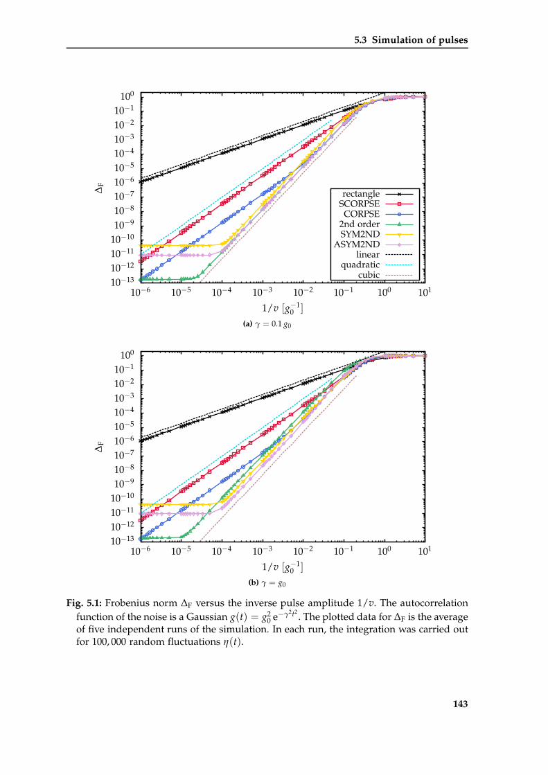
5.3 Simulation of pulses
10−1310−1210−1110−1010−910−810−710−610−510−410−310−210−1
100
10−6 10−5 10−4 10−3 10−2 10−1 100 101
∆F
1/v [g−10 ]
rectangleSCORPSE
CORPSE2nd orderSYM2ND
ASYM2NDlinear
quadraticcubic
(a) γ = 0.1 g0
10−1310−1210−1110−1010−910−810−710−610−510−410−310−210−1
100
10−6 10−5 10−4 10−3 10−2 10−1 100 101
∆F
1/v [g−10 ]
(b) γ = g0
Fig. 5.1: Frobenius norm ∆F versus the inverse pulse amplitude 1/v. The autocorrelationfunction of the noise is a Gaussian g(t) = g2
0 e−γ2t2. The plotted data for ∆F is the average
of five independent runs of the simulation. In each run, the integration was carried outfor 100, 000 random fluctuations η(t).
143
Chapter 5 Pulses for Pure Dephasing
ferent values γ = 0.1 g0 (upper panel) and γ = g0 (lower panel) of the decay rate γ. For
large values of 1/v, a saturation of the Frobenius norm ∆F is observed because there is
almost no overlap between an ideal pulse and a real pulse when the pulse amplitude is
small. This corresponds to the limit v → 0, where the trace in Eq. (5.7) vanishes and the
Frobenius norm acquires its maximum value ∆F =√
2. By decreasing 1/v, a characteris-
tic power law ∆F ∼ 1/vm+1 is revealed where m is the order of the pulse, see Eq. (1.12)
in Sect. 1.6. This is accomplished by all pulses, except the CORPSE pulse. It represents a
positive exception and behaves like a second order pulse for intermediate values of 1/v.
This behavior is rather incidental and implies that the CORPSE pulse makes second or-
der corrections vanish for a limited range of the parameter v. For small values of 1/v, it
performs like a first order pulse as to be expected. But it still outperforms the SCORPSE
pulse significantly. Thus, the CORPSE pulse has to be preferred over the SCORPSE pulse
in first order. The qualitative differences between the two studied decay rates γ = 0.01 g0
and γ = g0 are negligible.
In second order, the influence of the decay rate is more distinctive. For a slowly decaying
Gaussian g(t), the second order pulse optimized for a classical bath is comparable to
the ASYM2ND pulse optimized for a quantum bath. With increasing decay rate γ, the
ASYM2ND pulse clearly outperforms all other second order pulses. The failure of the
pulse optimized for a classical bath can be explained by recalling its derivation. It involves
the two leading orders of the Magnus expansion [SFPU12, Sti12] which is only a good
approximation as long as g(t) decays slowly. For a fast decaying autocorrelation function,
the leading orders of the Magnus expansion do not capture all the relevant physics. The
plateaus observed for very small values of 1/v are induced by the limited accuracy of
the pulse amplitudes and switching instances, see Tab. F.1 in Appendix F. More precisely,
the minimum acquired by the Frobenius norm for small values of 1/v scales roughly
linearly with the precision of the pulse. In Fig. 5.1, this behavior is depicted by the second
order pulse optimized for a classical bath. The quantum SYM2ND and ASYM2ND pulses
perform slightly worse because of their more complex structure.
The numerical results for an exponentially decaying autocorrelation function are presented
in Fig. 5.2. Only the unshaped rectangle behaves linearly as expected. All pulses of first and
second order reveal a rather surprising behavior expressed by the power law ∆F ∼ 1/v3/2
involving an unexpected half-integer value 3/2 for the exponent. In the upper panel of
Fig. 5.2, power-laws with exponents > 3/2 can still be estimated for a very limited interval
of 1/v. If the autocorrelation function of the noise decays faster (lower panel), these regions
vanish completely and ∆F ∼ 1/v3/2 is the only identifiable power law. From our point of
view, the occurrence of half-integer exponents is a unique feature which has not been
mentioned in the literature so far. Most likely, this untypical behavior has to be accounted
144
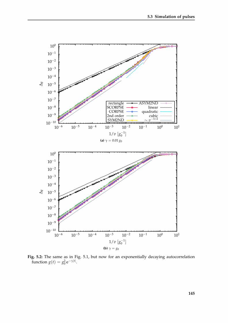
5.3 Simulation of pulses
10−10
10−9
10−8
10−7
10−6
10−5
10−4
10−3
10−2
10−1
100
10−6 10−5 10−4 10−3 10−2 10−1 100 101
∆F
1/v [g−10 ]
rectangleSCORPSE
CORPSE2nd orderSYM2ND
ASYM2NDlinear
quadraticcubic
∼ v−3/2
(a) γ = 0.01 g0
10−10
10−9
10−8
10−7
10−6
10−5
10−4
10−3
10−2
10−1
100
10−6 10−5 10−4 10−3 10−2 10−1 100 101
∆F
1/v [g−10 ]
(b) γ = g0
Fig. 5.2: The same as in Fig. 5.1, but now for an exponentially decaying autocorrelationfunction g(t) = g2
0 e−γ|t|.
145
Chapter 5 Pulses for Pure Dephasing
to the cusp in g(t). We come back to this issue in the next section, where we present an
analysis of ∆F based on AHT.
We close this section with some short remarks on the numerics. During our studies it
turned out that the influence of the discretization of the t-axis is crucial. The switching
instances as well as the amplitudes of the pulses have to be represented as exactly as pos-
sible. Otherwise, unexpected plateaus emerge in the Frobenius norm. Then, the expected
power laws cannot be detected because ∆F already saturates for fairly large values of 1/v.
The observed limitations correspond roughly to the accuracy of the implementation of the
pulses. This is prevented by employing a special discretization scheme of the t-axis. For
each constant segment of the pulse, the t-axis is split into a fixed number of intervals lead-
ing to a segment-depending value of ∆t. Thereby, the switching instances of the pulses
can be represented exactly. Compared to the pulse amplitude v(t), the supporting points
of the fluctuations η(t) are shifted by half a time interval ∆t. To reduce the integration er-
ror further, all time-evolution operators are represented by fourth order commutator-free
exponential time propagators (CFETs) as introduced by Alvermann et al. [AF11, AFL12].
The observations made in our numerics also have a considerable impact on the experiment
implying that the pulses have to be implemented with high precision. Only then, a reliable
performance can be expected. This knowledge may also be used for the design of new
pulses. For example, one could establish an additional constraint so that the switching
instances would be a multiple integer of each other. Then, a fixed value of ∆t could be
used for all segments of the pulse. Furthermore, rational numbers as switching instances
would be helpful.
146
5.4 Average Hamiltonian theory
5.4 Average Hamiltonian theory
In the following, we derive an analytic expression for the Frobenius norm ∆F. Thereby,
we are able to analyze the influence of the shape of g(t) on ∆F. The theory is based on
the Magnus expansion of the time-evolution operator [Mag54, BCOR09, AF11] which was
already employed for the AHT introduced in Chapter 3.
5.4.1 Analytical expression for the Frobenius norm
We start by further simplifying the Frobenius norm (5.7). For the time evolution under
the real pulse we recall the ansatz Ure(τp, 0) = Pτp · Uc(τp, 0) from Eq. (1.11). This product
ansatz decomposes Ure(τp, 0) into an ideal rotation Pτp times a correcting factor Uc(τp, 0)
induced by the coupling between spin and bath. This ansatz is well justified because it was
used to design the pulses investigated in the present thesis [PKRU09, SFPU12, Sti12]. The
ideal rotation Pτp as well as the correction Uc(τp, 0) fulfill a Schrödinger equation. For the
latter, the formal solution is given by
Uc(τp, 0) = T[
e− i∫ τp
0 dt H(t)
](5.8)
with the transformed Hamiltonian
H(t) := P†t H(t)Pt . (5.9)
Thus, the correction Uc(τp, 0) depends solely on the coupling between spin and bath. The
operator Pt with t ≤ τp represents an ideal rotation of the central spin, see next section. For
t = τp, the operator Pt corresponds to an ideal π-pulse around the x-axis. By exploiting
the unitarity of Pτp and the properties of the trace, all ideal rotations in ∆F cancel and the
Frobenius norm reduces to
∆2F = 2
1 − 1
3 ∑α=x,y,z
Tr(
ρα0Uc (τp, 0)ρα
0U†c (τp, 0)
) . (5.10)
The correcting factor Uc(τp) := Uc(τp, 0) is evaluated within the Magnus expansion. With-
out loss of generality, one may write
Uc(τp) = e− i~µ·~σ (5.11a)
147
Chapter 5 Pulses for Pure Dephasing
because the Magnus expansion ~µ is always linear in the Pauli matrices σα for a two-level
system, see Sect. 3.2 for comparison. At this point, no further assumptions have to be
made for ~µ. By exploiting the properties of the Pauli matrices explicitly, one obtains a
non-exponential representation of Eq. (5.11a)
Uc(τp) = 1 · cos |~µ| − i sin |~µ| · ~µ~σ|~µ| . (5.11b)
For a single value of α, the trace in Eq. (5.10) is given as
Tr(
ρα0Uc (τp)ρ
α0U†
c (τp))= cos2 |~µ|+ sin2 |~µ|
|~µ|2 · µ2α, (5.12)
with µ2α denoting the component α of ~µ. After carrying out the sum over all components
α, the squared Frobenius norm acquires the simple form
∆2F =
43
[1 − cos2 |~µ|
]. (5.13)
5.4.2 Magnus expansion
In the previous section, the formal notation ~µ was introduced as place holder for the Mag-
nus expansion. Now, we have to derive the expansion for the semiclassical Hamiltonian
H(t) containing the coupling between spin and bath (5.2b). To keep this section short, the
following derivation is restricted to the Hamiltonian Htot as defined in Eq. (5.1). A more
general derivation is given in Refs. [PKRU09, SFPU12, Sti12].
For an ideal rotation around the x-axis, the rotation operator is given as
Pt = e− i σx ψ(t)2
= 1 · cosψ (t)
2− i σx · sin
ψ (t)
2
(5.14)
where
ψ(t) := 2t∫
0
dt′ v(t′). (5.15)
Consequently, the expression for the transformed Hamiltonian (5.9) reads
H = η (t) sin ψ (t) · σy + η (t) cos ψ (t) · σz. (5.16)
148
5.4 Average Hamiltonian theory
Now, we address the Magnus expansion of Uc(τp) which is encoded in the vector
~µ = ∑k
~µ(k). (5.17)
Here, the sum runs over all required orders ~µ(k) of the expansion. This corresponds to
an expansion in the pulse duration τp because the k-th order of the Magnus expansion
induces contributions ~µ(k) ∼ τkp. As explained in Chapter 3, the time ordering in Eq. 5.8 is
simply neglected in leading order of the Magnus expansion. By comparing Eqs. (5.8) and
(5.11a), one obtains two non-zero contributions
µ(1)y =
τp∫
0
dt η (t) sin ψ (t) (5.18a)
µ(1)z =
τp∫
0
dt η (t) cos ψ (t) . (5.18b)
In second order, one has to evaluate the commutator [H(t1), H(t2)], see Appendix D. The
only non-vanishing contribution is given by
µ(2)x =
τp∫
0
dt1
τp∫
0
dt2 η (t1) η (t2) sin[ψ (t1)− ψ (t2)
]. (5.19)
Finally, the average of the squared Frobenius norm ∆2F with respect to all fluctuations η(t)
has to be calculated. This is also carried out in our numerical simulation, see Sect. 5.3.
Analytically, the calculation of the average with respect to η(t) corresponds to
∣∣~µ∣∣2 ≡ Tr
[Uc (τp)ρα
0U†c (τp)
]. (5.20)
Thereby, the averaged expression obtained from the first order contributions of the Magnus
expansion (5.18) reads
(µ(1)y
)2
+
(µ(1)z
)2
=
τp∫
0
dt1
τp∫
0
dt2 g (t1 − t2) cos[ψ (t1)− ψ (t2)
]. (5.21)
This expression induces contributions ∆2F ∼ 1/v2 and higher due to the presence of the
autocorrelation function g(t). Consecutively, the average (~µ(2))2 of the second order of the
Magnus expansion (5.19) induces terms which are of order 1/v4 and higher. Since we are
searching for a contribution ∆2F ∼ 1/v3, we do not have to take the second order of the
Magnus expansion into account.
149
Chapter 5 Pulses for Pure Dephasing
From a first guess, one might suppose that odd powers of 1/v in ∆2F could be induced
by contributions ∼ µ(1)α µ
(2)β origination from a combination of the first and the second
order of the Magnus expansion. In fact, such terms arise during the analytical evaluation
of Uc (τp)ρα0U†
c (τp). But they do not contribute under the trace because they are linear
in the Pauli matrices. This fact is also embedded in our final expression for the Frobenius
norm (5.13). The first order of the Magnus expansion is proportional to σy and σz, while the
second order only features a single contribution proportional to σx. Hence, a combination
of the first and second order cannot emerge from |~µ|.
Alternatively to Eq. (5.20), one might pursue a different strategy by averaging the Magnus
expansion of the correction Uc(τp, 0)
~µ ≡ Tr Uc(τp). (5.22)
Compared to Eq. (5.20), the average would be carried out at an earlier stage of our analyt-
ical derivation. Thus, the simple average ~µ of the Magnus expansion ~µ does not capture
all occurring contributions. For example, only contributions linear in the mean value η(t)
would be induced by the leading order of the Magnus expansion. The correlation function
g(t) of the noise would not appear.
5.4.3 Unexpected contributions for autocorrelation functions
displaying a cusp at t = 0
In the following, we evaluate the averaged expression from Eq. (5.21) for an exponential
autocorrelation function g(t) = g20 e−γ|t| or - more general - an autocorrelation function
whose leading-order expansion at t = 0 is given by
g (t) = g20(1 − γ |t|
)+O(t2). (5.23)
The second term characterizes the cusp at t = 0 and will induce the ∆2F ∼ 1/v3-power law
as we show below.
In leading order of g(t), one obtains the contribution
I1 = g20
τp∫
0
dt1
τp∫
0
dt2 cos[ψ (t1)− ψ (t2)
]∼(
1v
)2
(5.24)
which is only non-zero for an unshaped pulse of finite length. By applying the addition
150
5.4 Average Hamiltonian theory
theorem to cos(a + b), Eq. 5.24 reduces to two one-dimensional integrals
I1 = g20
τp∫
0
dt cos ψ (t)
2
+ g20
τp∫
0
dt sin ψ (t)
2
(5.25)
which vanish for pulses of first order and higher by definition [SFPU12, Sti12]. Conse-
quently, we have to claim that
0 ≡τp∫
0
dt sin ψ (t) (5.26a)
0 ≡τp∫
0
dt cos ψ (t) (5.26b)
when shaping pulses of first order. Next, we consider the linear order of g(t) implying
I3/2 = −g20γ
τp∫
0
dt1
τp∫
0
dt2 |t1 − t2| cos[ψ (t1)− ψ (t2)
]∼(
1v
)3
. (5.27)
Thereby, the candidate leading to a contribution ∆2F ∼ 1/v3 has been identified. In the next
section, the Frobenius norm is evaluated for the CORPSE and SCORPSE pulse. This serves
as a final verification of our AHT. We underline that the extinction of the latter expression
is in general not proposed in the derivation of shaped pulses. Hence, one has to demand
that the supplemental condition
0 ≡τp∫
0
dt1
τp∫
0
dt2 |t1 − t2| cos[ψ (t1)− ψ (t2)
](5.28)
has to be accomplished in addition to Eqs. (5.26) to improve pulses of first order or higher.
The occurrence of this new condition has to be attributed to the cusp in the autocorrelation
function g(t) at t = 0 which induces the odd orders in the expansion (5.23). Furthermore,
one has to employ the correct strategy when calculating the average over all random fluc-
tuations. If the correction Uc(τp) is averaged alone, the expression in Eq. (5.21) will only
depend on the squared mean value of the fluctuations and not on g(t). Since the mean
value is set to zero, the AHT for ∆2F does not contain odd powers of 1/v in this case.
To our knowledge, the additional condition (5.28) as well as the observation of contribu-
tions ∆F ∼ 1/v3/2 has not been described in the literature so far. This unique feature occurs
as soon as the autocorrelation function of the noise exhibits a cusp at t = 0, for example
in Ornstein-Uhlenbeck processes. In this case, the strategy for shaping pulses has to be
151
Chapter 5 Pulses for Pure Dephasing
revised. In the framework of dynamic decoupling, a similar behavior was recently found
by Wang and Liu [WL13]. They showed that a sequence of pulses can only suppress the
decoherence up to a limited order depending on the high-frequency cutoff of the noise.
For an Ornstein-Uhlenbeck-type noise, their results are in agreement with our findings for
the Frobenius norm under a single pulse.
Only when the conditions in Eqs. (5.26) and (5.28) are simultaneously fulfilled, a shaped
first order pulse displays the expected behavior. However, it has been proven that both
conditions cannot be accomplished at the same time, see Appendix G. Hence, one should
stick to first order pulses and try to minimize Eq. (5.28) in addition to the extinction of
Eqs. (5.26). Thereby, the prefactor of the power law is minimized. To our present knowl-
edge, the optimal solution is given by the well-known SCORPSE pulse [Fau13]. Better
pulses have not been identified so far. If there is no linear order in g(t), one can of course
proceed as usual.
By considering higher orders of g(t) and the Magnus expansion, subsequent orders of
∆2F can easily be deduced. Contributions ∆2
F ∼ 1/v4 are obtained from the averaged first
order of the Magnus expansion (5.21) in combination with the quadratic order of g(t) and
from the averaged second order of the Magnus expansion in combination with the constant
order of g(t). The systematic expansion may be pushed further to reveal odd contributions
of higher orders. For example, Eq. (5.21) induces terms ∆2F ∼ 1/v5 in combination with the
cubic order of g(t). Thus, more and more so far unknown conditions arise with increasing
order of the pulse. This is already a sophisticated task in first order so that one should
refrain from deriving pulses of second order and higher when odd terms are present in
the expansion of the autocorrelation function.
Our analytical results for the Frobenius norm may also be used to draw conclusions from
a measurement of the pulse fidelity on the type of noise of the bath. For example, an
experimental investigation of pulses could reveal an unusual behavior in dependence of
the inverse pulse amplitude 1/v or the pulse duration τp. In the measured quantity, this
may be expressed by contributions proportional to odd or half-integer powers of 1/v or
τp. Consequently, the autocorrelation function g(t) should likely feature a cusp at t = 0
according to our results. This would imply the presence of highly energetic processes in
the bath which dominate the short-time behavior of the noise. Vice versa, the presence
of a soft high-energy cutoff ∼ 1/ω2 in the measured noise spectrum of the bath would
indicate that the efficiency of pulses is limited. In particular, this would imply that second
order pulses do not lead to a significant improvement compared to first order pulses.
152
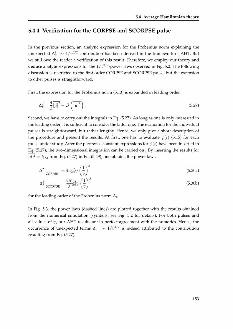
5.4 Average Hamiltonian theory
5.4.4 Verification for the CORPSE and SCORPSE pulse
In the previous section, an analytic expression for the Frobenius norm explaining the
unexpected ∆2F ∼ 1/v3/2 contribution has been derived in the framework of AHT. But
we still owe the reader a verification of this result. Therefore, we employ our theory and
deduce analytic expressions for the 1/v3/2-power laws observed in Fig. 5.2. The following
discussion is restricted to the first order CORPSE and SCORPSE pulse, but the extension
to other pulses is straightforward.
First, the expression for the Frobenius norm (5.13) is expanded in leading order
∆2F =
43
∣∣~µ∣∣2 +O
(∣∣~µ∣∣4)
. (5.29)
Second, we have to carry out the integrals in Eq. (5.27). As long as one is only interested in
the leading order, it is sufficient to consider the latter one. The evaluation for the individual
pulses is straightforward, but rather lengthy. Hence, we only give a short description of
the procedure and present the results. At first, one has to evaluate ψ(t) (5.15) for each
pulse under study. After the piecewise constant expressions for ψ(t) have been inserted in
Eq. (5.27), the two-dimensional integration can be carried out. By inserting the results for
|~µ|2 = I3/2 from Eq. (5.27) in Eq. (5.29), one obtains the power laws
∆2F
∣∣∣CORPSE
= 4πg20γ
(1v
)3
(5.30a)
∆2F
∣∣∣SCORPSE
=8π
3g2
0γ
(1v
)3
(5.30b)
for the leading order of the Frobenius norm ∆F.
In Fig. 5.3, the power laws (dashed lines) are plotted together with the results obtained
from the numerical simulation (symbols, see Fig. 5.2 for details). For both pulses and
all values of γ, our AHT results are in perfect agreement with the numerics. Hence, the
occurrence of unexpected terms ∆F ∼ 1/v3/2 is indeed attributed to the contribution
resulting from Eq. (5.27).
153
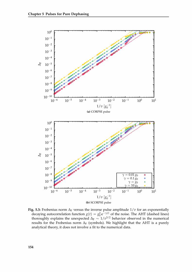
Chapter 5 Pulses for Pure Dephasing
10−10
10−9
10−8
10−7
10−6
10−5
10−4
10−3
10−2
10−1
100
10−6 10−5 10−4 10−3 10−2 10−1 100 101
∆F
1/v [g−10 ]
(a) CORPSE pulse
10−10
10−9
10−8
10−7
10−6
10−5
10−4
10−3
10−2
10−1
100
10−6 10−5 10−4 10−3 10−2 10−1 100 101
∆F
1/v [g−10 ]
γ = 0.01 g0γ = 0.1 g0
γ = g0γ = 10 g0
(b) SCORPSE pulse
Fig. 5.3: Frobenius norm ∆F versus the inverse pulse amplitude 1/v for an exponentiallydecaying autocorrelation function g(t) = g2
0 e−γ|t| of the noise. The AHT (dashed lines)thoroughly explains the unexpected ∆F ∼ 1/v3/2 behavior observed in the numericalresults for the Frobenius norm ∆F (symbols). We highlight that the AHT is a purelyanalytical theory, it does not involve a fit to the numerical data.
154
Conclusion
In this thesis, we investigated the spin dynamics in the central spin model with and with-
out external magnetic field. Experimentally, the central spin model describes the deco-
herence of a single electron spin confined in a quantum dot which is dominated by the
hyperfine interaction between the electron spin and the surrounding nuclear spins in the
dot. We tackled the problem on three different levels: A full treatment of the quantum
model in the framework of DMRG, a semiclassical model involving a replacement of the
bath by a classical random field, and by solving the classical equations of motion.
The numerical treatment on the level of DMRG captures the full hyperfine interaction in
the central spin model. Compared to exact diagonalization and Bethe ansatz techniques,
the number of accessible bath spins is at least one order of magnitude larger. Therefore,
we demonstrated how DMRG can be efficiently adapted for a starlike cluster of spins as
defined by the topology of the central spin model. The exact calculation of the trace of
the observables at infinite temperature is enabled by purifying the initial state at the cost
of doubling the size of the bath. For calculating the real-time evolution in the framework
of DMRG, three different approaches were introduced and tested. Thereby, the adaptive
method based on the Trotter-Suzuki decomposition of the time-evolution operator was
identified to work best for our purposes. Even in second order, the Trotter-Suzuki de-
composition has proven to yield good results up to intermediate times t ≈ 30-50 J−1q . In
general, it is not required to employ the fourth order decomposition. Due to the moder-
ately growing total discarded weight and acceptable run times, up to N ≈ 1000 bath spins
can be treated on intermediate time scales.
In contrast, Krylov vectors do not suffer from the Trotter-Suzuki error so that they ex-
ceed the accuracy of the Trotter-Suzuki decomposition on the short-time scale. But they
fail for larger times because of the fast growing total discarded weight and the strongly
increasing amount of CPU time. In addition, we implemented the real-time evolution on
the basis of Chebychev polynomials. However, this approach cannot be recommended due
to extremely fast growing total discarded weight. The comparison with the two other ap-
proaches revealed that it already fails for small numbers of bath spins. This has to be
accounted to the special symmetry of the central spin model: Due to the starlike structure,
155
Conclusion
a perturbation created at the site of the central spin spreads immediately over the whole
cluster of spins. But the performance of the Chebychev expansion might be improved by
including the doubling of the number of coefficients as suggested in Sect. 2.5.4. Thereby,
one could also avoid the permanent targeting of the initial state.
Subsequently, we presented a detailed analysis of the performance of the real-time evo-
lution with DMRG based on the Trotter-Suzuki decomposition. As a first application, the
influence of the number of bath spins on the short-time dynamics in the central spin model
was investigated. Without any external field, the autocorrelation function of the central
spin never exhibits a complete decay and the autocorrelation function of the Overhauser
field is almost static. An external field induces an additional precession of the central spin
and the bath spins. This causes the dephasing of the central spin in the spin directions
perpendicular to the external field. In contrast, a finite external field suppresses the relax-
ation in the spin direction parallel to the external field. By increasing the external field, a
crossover from a smooth to an oscillating decay of the transverse autocorrelation functions
occurs.
Compared to other approaches applicable for large bath sizes, our ansatz based on the
DMRG fully captures the dynamics in the quantum central spin model for arbitrary ex-
ternal fields while cluster expansions and solutions of non-Markovian master equations
always require a finite external field. Moreover, cluster expansions usually involve the
secular approximation where spin flips between the central spin and the bath spins are
neglected. Furthermore, an intrinsic dynamics of the bath is induced by dipolar couplings
between the bath spins which are usually distributed randomly. A well-defined distribu-
tion of the couplings is not used. Thus, the employed model cannot be compared directly
to the central spin model studied in the present thesis.
In contrast, master equations are employed to study the central spin dynamics in the
central spin model. With respect to our distribution of the coupling constants, the latest
non-perturbative master equation solution by Barnes et al. [BCDS12] requires a finite ex-
ternal field which has to be at least of the order of the energy scale Jq for N ≈ 1000 bath
spins. In addition, the accessible time scale is limited by the largest coupling constant. We
stress that there is no such restriction in our DMRG calculations. For N ≈ 1000 bath spins,
DMRG yields good results up to t ≈ 25-30 J−1q while the non-perturbative solution of the
master equation is restricted to t ≈ 18 J−1q which is significantly smaller. Hence, the DMRG
outperforms the non-perturbative solution of the master equation also with respect to the
accessible time scales, see Appendix H for more details. Older master equation solutions,
for example the one presented in Ref. [FBN+08], require an even larger external field so
that the strength has to be a multiple of the energy scale Jq. The same restriction holds for
156
the perturbative approach presented in Ref. [CL04]. Consequently, these approaches de-
liver solutions valid only in the strong-field regime, where DMRG works extremely well
and the dynamics is essentially classical, see below.
Motivated by the results for the zero-field limit and by a simple analytic argument, we
introduced an effective semiclassical picture for the central spin problem. In the semiclas-
sical model, the bath is replaced by a classical Gaussian variable, while the central spin is
still treated on the quantum level. First, we introduced an average Hamiltonian theory for
the central spin based on the systematic Magnus expansion of the time-evolution operator.
Second, a numerical simulation of the central spin in the semiclassical model involving
a sampling of the random fluctuations was carried out. Together with DMRG, we were
able to show that - depending on the exact value of t - both the semiclassical as well as
the quantum result converge towards the static bath approximation for already a mod-
erate number of N & 100 bath spins. But the comparison with the DMRG results up to
intermediate times revealed that a separate treatment of the conserved quantities in the
numerical simulation of the semiclassical model is crucial. When the conserved total spin
is treated separately, a nice agreement between the semiclassical and the quantum picture
is achieved in the zero-field limit up to intermediate times. However, this approach re-
quires the correlation function of the bath to be known from an external source. Moreover,
it does not fulfill the conservation of the total energy.
The latter was achieved by regarding the fully classical equations of motion. The numer-
ical solution of the classical equations of motion also comprises a consistent calculation
of the autocorrelation functions of the bath. In the zero-field limit, it turned out that the
dynamics of the central spin on the short-time scale is essentially classical as long as the
size of the bath is not too small (N & 100 bath spins). For larger times, the influence of
quantum fluctuations increases. Compared to the classical description, they slightly reduce
the non-decaying fraction of the autocorrelation function of the central spin. In a finite ex-
ternal field, the accuracy of the classical approximation depends on the strength of the
external field. A qualitative description of the central spin dynamics is achieved always.
The agreement between the classical and the quantum description increases upon growing
external field. In the strong-field limit, both qualitative and quantitative agreement is ac-
quired. With respect to the Overhauser field, the differences between the classical and the
quantum picture are more pronounced. As long as the external field is weak or not present
at all, the classical description of the Overhauser field is still fairly good. However, discrep-
ancies arise in the spin directions perpendicular to the external field when the strength of
the field is increased. For large fields, the classical bath spins only feel an effective field
of the central spin due to its very fast precession. Hence, the autocorrelation functions of
the classical Overhauser field in spin directions perpendicular to the external field do not
157
Conclusion
display any oscillations as their quantum counterparts. Instead, they decay smoothly to
zero. But concerning the static limit, our observations suggest that the classical as well as
the quantum description of the Overhauser field will coincide if the number of bath spins
is sufficiently large.
Finally, we considered an application of the semiclassical model and investigated op-
timized pulses suppressing the dephasing of the central spin. Thereby, an unexpected
∆F ∼ 1/v3/2 behavior of the Frobenius norm was revealed for pulses of first order and
higher if the autocorrelation function of the noise displays a cusp at t = 0, for instance
due to an Ornstein-Uhlenbeck process. On the level of average Hamiltonian theory, we
verified that this unusual behavior has to be attributed to the cusp in the autocorrelation
function of the noise. To diminish the effect of the half-integer contribution, we derived an
additional condition to be fulfilled by pulses of first order and higher. But the contribution
of the half-integer order can only be minimized, it cannot be eliminated. This could be
established rigorously.
Outlook
With the DMRG code for the quantum model and the corresponding codes for the semi-
classical and classical model, we have developed a wide selection of powerful tools for
investigating the spin dynamics in the central spin model. In the following, we suggest
several applications of the existing tools and some possible future extensions.
So far, a generic uniform distribution of the coupling constants was used for the proof-of-
principle investigation presented in this thesis. Without any additional effort, the existing
codes can be employed to study the influence of various types of distributions on the spin
dynamics. Thereby, one can account for more realistic shapes of the central spin wave
function and parameters extracted from experiment, see for instance Ref. [SKL03, HA14].
Moreover, one may also investigate the spin dynamics for anisotropic coupling constants
as discussed in Ref. [HA14].
Additional pulses can be implemented easily in the random noise simulation of the semi-
classical model. In particular, the simulation may serve as a nice benchmark for pulses
optimized specifically for an Ornstein-Uhlenbeck type noise. Future work could also com-
prise the numerical simulation of pulse sequences from dynamic decoupling or pulses and
pulse sequences in the framework of the classical equations of motion or in the framework
of DMRG, see below.
158
With respect to the real-time evolution based on the Chebychev expansion, one should def-
initely implement the doubling of the coefficients as described in Sect. 2.5.4. Additionally,
other orthogonal polynomials such as Hermite polynomials may be employed for the
calculation of the real-time evolution. A comparison of the advantages and disadvantages
of different orthogonal polynomials would certainly be worthwhile.
Several other extensions of the DMRG code are feasible. Starting from a purified initial
state, finite temperatures may be reached by cooling the system via a time evolution in
imaginary time. The implementation is straightforward, since the required routines may
be taken over from the time evolution based on the Trotter-Suzuki decomposition. How-
ever, the central site has to be purified as well which may imply a certain caveat. Further-
more, one could study the influence of an intrinsic dynamics in the bath induced by a
dipolar interaction between the bath spins. To avoid dipolar couplings going beyond near-
est neighbor interaction, one should consider an exemplary dipolar interaction where the
bath spins form a linear chain. A non-interacting linear alignment of the bath spins has
already been assumed in the DMRG setup of system and environment block. Hence, just
the corresponding interaction terms would have to be added to the Hamiltonian.
Another worthwhile - but ambitious - extension is the simulation of pulses or even pulse
sequences in the framework of time-dependent DMRG. While ideal pulses may be realized
without great effort in the existing code, some severe changes would be required for the
implementation of real pulses of finite length. Due to the Trotter-Suzuki decomposition,
the implementation of time-dependent Hamiltonians is straightforward because only the
local time-evolution operators must be modified. But a real pulse implies a continuous
change of the magnetization of the superblock state. Consequently, the magnetization is
not a conserved quantity anymore and the corresponding good quantum number cannot
be used to label the basis of the blocks. This would result in a significant decrease of the
performance of the algorithm because the block structure of the matrices would be gone.
Consequently, the accessible number of bath spins and maximum time scales would have
to be reduced to compensate the loss of performance.
159


Appendix

Appendix A
Transformation of the DMRG Superblock State
In this appendix, an example for the transformation of the state vector in DMRG is pre-
sented. The implementation of such transformations was first suggested by White [Whi96].
Applied during the finite size algorithm introduced in Sect. 2.2.2, they speed up the cal-
culation of the target state by improving the initial guess for iterative procedures. The
target state of the previous block configuration is transformed approximately to the basis
of the next DMRG step and can thus be used as starting point of, for example, the Lanczos
algorithm to calculate the ground state. Furthermore, they are essential for the sweeps
occurring in all methods for the real-time evolution, see Sect. 2.4. In the adaptive approach
based on the TS decomposition, the local time-evolution operators are applied during the
transformation of the superblock state, see Sect. 2.4.2.
In the following, we depict the scenario where the system block is left and the environment
block is right. The transformation extracts the bath site Pl+1 from the environment block
EN−l and integrates it into the system block Sl. This corresponds to a single step in the
half-sweep from left to right. Before the transformation, the state of the superblock has the
form
|Ψ〉 = ∑ml ,mN−l
Ψml ,mN−l|ml〉L |mN−l〉R , (A.1)
where ml and mN−l are the quantum numbers of the left and right block, as denoted by
the indices of the basis vectors. The indices of the quantum numbers denote the number
of bath spins in the respective block. As before, the bar indicates that the basis of the right
block incorporates the central spin.
At first, we insert the truncated basis ∑ml|ml〉 〈ml | ≈ 1 to reduce the basis of the system
163
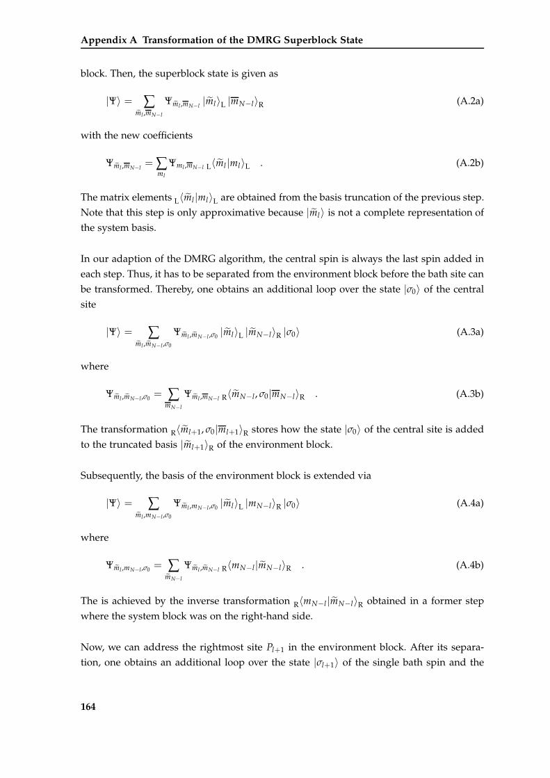
Appendix A Transformation of the DMRG Superblock State
block. Then, the superblock state is given as
|Ψ〉 = ∑ml ,mN−l
Ψml ,mN−l|ml〉L |mN−l〉R (A.2a)
with the new coefficients
Ψml ,mN−l= ∑
ml
Ψml ,mN−l L〈ml |ml〉L . (A.2b)
The matrix elements L〈ml|ml〉L are obtained from the basis truncation of the previous step.
Note that this step is only approximative because |ml〉 is not a complete representation of
the system basis.
In our adaption of the DMRG algorithm, the central spin is always the last spin added in
each step. Thus, it has to be separated from the environment block before the bath site can
be transformed. Thereby, one obtains an additional loop over the state |σ0〉 of the central
site
|Ψ〉 = ∑ml ,mN−l,σ0
Ψml ,mN−l ,σ0 |ml〉L |mN−l〉R |σ0〉 (A.3a)
where
Ψml ,mN−l,σ0 = ∑mN−l
Ψml ,mN−l R〈mN−l, σ0|mN−l〉R . (A.3b)
The transformation R〈ml+1, σ0|ml+1〉R stores how the state |σ0〉 of the central site is added
to the truncated basis |ml+1〉R of the environment block.
Subsequently, the basis of the environment block is extended via
|Ψ〉 = ∑ml ,mN−l,σ0
Ψml ,mN−l ,σ0 |ml〉L |mN−l〉R |σ0〉 (A.4a)
where
Ψml ,mN−l,σ0 = ∑mN−l
Ψml ,mN−l R〈mN−l|mN−l〉R . (A.4b)
The is achieved by the inverse transformation R〈mN−l|mN−l〉R obtained in a former step
where the system block was on the right-hand side.
Now, we can address the rightmost site Pl+1 in the environment block. After its separa-
tion, one obtains an additional loop over the state |σl+1〉 of the single bath spin and the
164
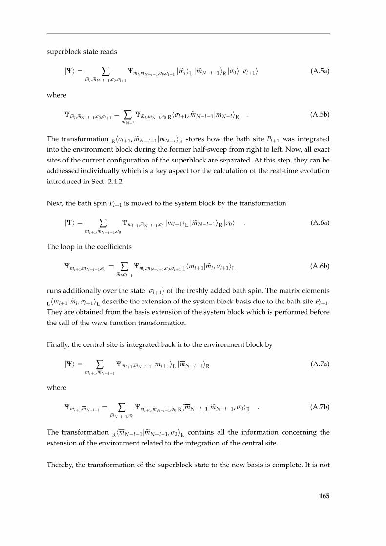
superblock state reads
|Ψ〉 = ∑ml ,mN−l−1,σ0,σl+1
Ψml ,mN−l−1,σ0,σl+1|ml〉L |mN−l−1〉R |σ0〉 |σl+1〉 (A.5a)
where
Ψml ,mN−l−1,σ0,σl+1= ∑
mN−l
Ψml ,mN−l,σ0 R〈σl+1, mN−l−1|mN−l〉R . (A.5b)
The transformation R〈σl+1, mN−l−1|mN−l〉R stores how the bath site Pl+1 was integrated
into the environment block during the former half-sweep from right to left. Now, all exact
sites of the current configuration of the superblock are separated. At this step, they can be
addressed individually which is a key aspect for the calculation of the real-time evolution
introduced in Sect. 2.4.2.
Next, the bath spin Pl+1 is moved to the system block by the transformation
|Ψ〉 = ∑ml+1,mN−l−1,σ0
Ψml+1,mN−l−1,σ0 |ml+1〉L |mN−l−1〉R |σ0〉 . (A.6a)
The loop in the coefficients
Ψml+1,mN−l−1,σ0 = ∑ml ,σl+1
Ψml ,mN−l−1,σ0,σl+1 L〈ml+1|ml , σl+1〉L (A.6b)
runs additionally over the state |σl+1〉 of the freshly added bath spin. The matrix elements
L〈ml+1|ml , σl+1〉L describe the extension of the system block basis due to the bath site Pl+1.
They are obtained from the basis extension of the system block which is performed before
the call of the wave function transformation.
Finally, the central site is integrated back into the environment block by
|Ψ〉 = ∑ml+1,mN−l−1
Ψml+1,mN−l−1 |ml+1〉L |mN−l−1〉R (A.7a)
where
Ψml+1,mN−l−1 = ∑mN−l−1,σ0
Ψml+1,mN−l−1,σ0 R〈mN−l−1|mN−l−1, σ0〉R . (A.7b)
The transformation R〈mN−l−1|mN−l−1, σ0〉R contains all the information concerning the
extension of the environment related to the integration of the central site.
Thereby, the transformation of the superblock state to the new basis is complete. It is not
165
Appendix A Transformation of the DMRG Superblock State
exact due to the involved basis truncation. But the DMRG truncation with respect to the
reduced density matrix keeps all important states so that the error should be of the order
of the discarded weight. Concerning the implementation, all required transformations de-
scribed above have to be stored during the runtime of the algorithm. This applies to all
basis truncations as well as to all basis extensions. The transformations for the half-sweep
from right to left and for the interchange of the left and the right block are closely related
to the presented example and can be adapted easily.
166
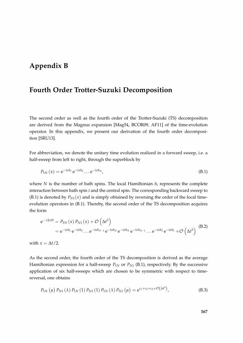
Appendix B
Fourth Order Trotter-Suzuki Decomposition
The second order as well as the fourth order of the Trotter-Suzuki (TS) decomposition
are derived from the Magnus expansion [Mag54, BCOR09, AF11] of the time-evolution
operator. In this appendix, we present our derivation of the fourth order decomposi-
tion [SRU13].
For abbreviation, we denote the unitary time evolution realized in a forward sweep, i.e. a
half-sweep from left to right, through the superblock by
P1N (x) = e−ixh1 e−ixh2 . . . e−ixhN , (B.1)
where N is the number of bath spins. The local Hamiltonian hi represents the complete
interaction between bath spin i and the central spin. The corresponding backward sweep to
(B.1) is denoted by PN1(x) and is simply obtained by reversing the order of the local time-
evolution operators in (B.1). Thereby, the second order of the TS decomposition acquires
the form
e− i 2xH = P1N (x) PN1 (x) +O(
∆t3)
= e−ixh1 e−ixh2 . . . e−ixhN−1 e−ixhN e−ixhN e−ixhN−1 . . . e−ixh2 e−ixh1 +O(
∆t3) (B.2)
with x = ∆t/2.
As the second order, the fourth order of the TS decomposition is derived as the average
Hamiltonian expression for a half-sweep P1N or PN1 (B.1), respectively. By the successive
application of six half-sweeps which are chosen to be symmetric with respect to time-
reversal, one obtains
P1N
(µ)
PN1 (λ) P1N (1) PN1 (1) P1N (λ) PN1(µ)= ec1+c2+c3+O(∆t5), (B.3)
167
Appendix B Fourth Order Trotter-Suzuki Decomposition
where the right-hand side results from the Magnus expansion. The operators ci in the
exponential read
c1 = 2Ω1(1 + λ + µ
)(B.4a)
c2 = Ω2
(λ2 − λ2 + µ2 − µ2
)= 0 (B.4b)
c3 = 2Ω3
(λ3 + µ3 + 1
)+ [Ω1, Ω2]
(1 + µ3 + 2λµ2 + 2µ2 − λ3 − 2λ2
), (B.4c)
where Ωn denotes the n-th order contribution of the Magnus expansion [AF11]. The first
order is given by the local decomposition of the Hamiltonian H
Ω1 =N
∑i=1
hi . (B.5)
The brackets in Eq. (B.4b) vanish by construction due to the time-reversal symmetry of the
sequence. For the same reason we know without calculation that there is no contribution
c4 ∼ ∆t4 [Hae76]. The brackets in Eq. (B.4c) vanish for µ = −1/ 3√
2 = λ so that Eq. (B.3)
corresponds to the desired time-evolution operator up to O(∆t5).
Now, we define
e−iH∆t = P1N
(α
∆t
2
)· PN1
(β
∆t
2
)· P1N
(γ
∆t
2
)· PN1
(γ
∆t
2
)
· P1N
(β
∆t
2
)· PN1
(α
∆t
2
)+O
(∆t5)
.(B.6)
for the fourth order of the TS decomposition. The coefficients
α =1
2 − 21/3 = β (B.7a)
γ = − 122/3 − 1
(B.7b)
are obtained by rescaling the solutions for λ and µ from Eqs. (B.4).
If the fourth order decomposition is used to calculate the real-time evolution with the
adaptive method, three back and forth sweeps are required to proceed one step ∆t in time.
After t/∆t applications, the TS error in fourth order accumulates to O(∆t4).
168
Appendix C
Purified States
In this appendix, we present an analytic argument that the time-evolution operator
U = e− i(Hr−Ha)∆t (C.1)
leaves a completely purified initial state |0〉 as defined in Eq. (2.59) unchanged. The Hamil-
tonian of the real spins is denoted by Hr, while Ha denotes the Hamiltonian for the aux-
iliary spins. They are both identical, but the auxiliary spins propagate backwards in time.
The following line of argument is taken from Ref. [SRU13] where we argued on the basis
of a simple toy model.
We consider a singlet state
|S1, S2〉 =1√
2S + 1
2S
∑i
(−1)i |S − i,− (S − i)〉 (C.2)
of two half-integer spins, for example two nearest neighbors taken from a chain. The
operators acting on site 1 and 2 are denoted by ~Si,r. A generic Hamiltonian for the two
spins is Hr = ~S1,r · ~S2,r. In addition, an auxiliary spin with operator ~Si,a is introduced for
each real spin.
The action of Hr on the initial state |S1, S2〉 is given as
Hr |S1, S2〉 = ~S1,r · ~S2,r |S1, S2〉 (C.3a)
= −~S1,a · ~S2,r |S1, S2〉 , (C.3b)
where the spin S1 has been swapped with its auxiliary antiparallel spin sitting on the same
site, see Eq. (2.59). Swapping the second spin with its auxiliary one cancels the minus sign
169
Appendix C Purified States
again so that the action of Hr on the initial state is given as
Hr |S1, S2〉 = ~S1,a · ~S2,a |S1, S2〉 . (C.3c)
The latter expression implies
Hr |S1, S2〉 = Ha |S1, S2〉 , (C.4)
where the Hamiltonian Ha = ~S1,a · ~S2,a acts on the auxiliary sites only. Hence, the action of
both Hamiltonians on the initial state |S1, S2〉 is the same.
Consequently, the action of the Hamiltonian
H = Hr − Ha (C.5)
on a purified initial state |0〉 is always zero because all contributions compensate each
other. For the application of the time-evolution operator U = e−iHt, this implies
e−i(Hr−Ha) |0〉 = |0〉 , (C.6)
which is valid as long as all real sites are prepared as singlets (or m = 0 triplets for
S = 1/2) with their corresponding auxiliary sites. The property (C.6) is destroyed if any
operator is applied to the real sites so that |0〉 is changed to a state different from a product
of singlets.
Note, however, that the advantage of using H = Hr − Ha depends on the topology. In a
chain with nearest-neighbor interactions, the benefit is largest because a local perturbation
at site j will be felt at site j + n only at the n-th application of H. In the star topology of
the central spin model the situation is different. Applying an operator to the central spin
and subsequently H destroys the singlet character already at every bath site.
170
Appendix D
Second Order Average Hamiltonian Theory
In Chapter 3, the first order of the average Hamiltonian theory for the semiclassical model
Hsc = ~η(t) · ~S0 has been derived. It is based on the leading order of the Magnus expansion
of the time-evolution operator. In the following, we include the subsequent order of the
Magnus expansion and derive the second order corrections of our average Hamiltonian
theory, see also Ref. [SRU13].
To this end, we recall the expression for the autocorrelation function 〈Sz0(t)S
z0(0)〉 prior to
averaging as given in Eq. (3.11). It is rewritten in the form
〈Sz0(t)S
z0(0)〉 =
112
+16
X (1) (D.1)
with
X (a) = 4π
∞∫
0
dv v2 cos (va) P (v) . (D.2)
Here, P (v) is a spherical probability distribution obeying the spin rotational symmetry of
the model. Hence, it depends on the modulus v = |~v| only. The previous expression for X
is generalized by replacing P(v) with the probability distribution of a single component of
~v, for example the z-component
p (vz) =∫∫∫
d3v P (v) δ (vz − v cos θ)
= 2π
∞∫
|vz |
dv vP (v) .(D.3)
This equation is differentiated with respect to vz and inserted into Eq. (D.2). Hence, one
171
Appendix D Second Order Average Hamiltonian Theory
obtains
X (a) = −2∞∫
0
dv v cos (va) p′ (v) . (D.4)
By partially integrating this expression with respect to a, it is reduced to
X (a) = p (a) + ap′ (a) (D.5)
where the Fourier transform p(a) =∫ ∞
−∞dv p(v) eiva of p(v) has been introduced. The
expression in Eq. (D.5) is a general representation of the non-constant part of the autocor-
relation function of the central spin (D.1). Just the Fourier transform p(a) remains to be
calculated, which is nothing else but the mean value of the exponential factor eiav.
In the following, we present how this expression is calculated and evaluated. The Magnus
expansion [Mag54, BCOR09] up to second order reads
U (t) = exp
−i
t∫
0
dt′ H(t′) +12
t∫
0
dt1
t1∫
0
dt2[H (t1) , H (t2)
]
. (D.6)
For a single spin-1/2, the Magnus expansion is always linear in the spin operators. Thus,
it can be written in the form
U (t) = e−i~v·~σ2 (D.7)
with
vx =
t∫
0
dt′ ηx(t′) +
12
t∫
0
dt1
t∫
0
dt2 ηy (t1) ηz (t2) sgn (t1 − t2) (D.8)
and cyclic in the components x, y and z. This expression is the desired argument of the
exponential in p(a), just the average
p (a) = eiavx (D.9)
with respect to all three components ηx, ηy, and ηz has yet to be calculated. By applying
the general identity
exp
t2∫
t1
dτ a (τ) η (τ)
= exp
12
t2∫
t1
dt
t2∫
t1
dτ a (t) g (t − τ) a (τ)
. (D.10)
172
valid for Gaussian fluctuations, the mean value can be evaluated analytically. In the con-
tribution resulting from the first order of the Magnus expansion, only the mean value for
ηx has to be calculated. Therefore, one obtains
exp
ia
t∫
0
dt′ ηx (t′)
x
= exp[−a2G (t)
](D.11)
where
G (t) =
t∫
0
dt1
t1∫
0
dt2 g (t1 − t2) (D.12)
is an even function as is g(t). For the contribution from the second order of the Magnus
expansion, the average with respect to ηy is carried out analytically
exp
ia2
t∫
0
dt1
t∫
0
dt2 ηy (t1) ηz (t2) sgn (t1 − t2)
y
= exp
− a2
8
t∫
0
dt1
t∫
0
dt′1 α(t1)g(t1 − t′1)α(t′1)
(D.13)
where
α (t1) :=t∫
0
dt2 sgn (t1 − t2) ηz (t2) (D.14)
still depends on ηz. After rearranging the integrals in the latter expression, the intermediate
result for p(a) from Eq. (D.9) can be written as
p (a) = e−a2G(t) · e−a28
∫ t0 dt2
∫ t0 dt′2 ηz(t′2)A(t′2,t2)ηz(t2)
z
. (D.15a)
The two integrations with respect to t1 and t′1 in A(t′2, t2) are carried out analytically and
one obtains
A(t′2, t2) :=t∫
0
dt1
t∫
0
dt′1 sgn(t′1 − t′2)g(t′1 − t1)sgn(t1 − t2)
= 2[
G(t2 − t) + G(t′2 − t)− 2G(t2 − t′2) + G(t2) + G(t′2)− G(t)]
.
(D.15b)
173
Appendix D Second Order Average Hamiltonian Theory
The average with respect to ηz still remains and cannot be calculated in a closed form
analytically, even though it is a Gaussian average. Thus, we introduce a simple numerical
approach based on the discretization of time t in D intervals of width ∆t = t/D. Then, the
average of ~ηz = (ηz(t1) . . . ηz(tN))⊤ is carried out with respect to an D-dimensional Gaus-
sian probability distribution and the integrals in the exponential are replaced by sums.
Consequently, the Fourier transform (D.15a) reads
p (a) =e−a2G(t)
√det M
∞∫
−∞
dDηz
(2π)D/2 e−12~η
⊤z M−1~ηz e−
12~η
⊤z P~ηz . (D.16)
The matrix M = (Mij) is the covariance matrix defined by
Mij := g(ti − tj), (D.17a)
while
Pij :=a2
4A(ti, tj)∆t2 (D.17b)
contains the correction of the second order. The discretized time steps of width ∆t = t/D
are given as
ti =
(i − 1
2
)t
D, i ∈ 1, . . . , D. (D.17c)
Note that the structure of the correction in Eq. (D.16) is also bilinear in ηz. Hence, the D-
dimensional integration is carried out easily and the final result for the Fourier transform
is given by
p (a) =1√
det (1+ PM)e−a2G(t) . (D.18)
In total, the second order of the AHT leads to a renormalization of the probability dis-
tribution by a factor 1/√
det (1+ PM). With the Fourier transform and Eqs. (D.1) and
(D.5), we have obtained the final expression for the autocorrelation function 〈Sz0(t)S
z0(0)〉
in second order AHT.
Concerning the numerical evaluation, only a rough discretization of t is sufficient. In prac-
tice, it turned out that D = 20-30 is an adequate number for evaluating Eq. (D.1) up to
t = 10. As an example, the effect of the second order AHT is illustrated for the exemplary
correlation function g(t) = 1/4 e−|t|/(8τ) in Fig. D.1. The renormalization of the probabil-
ity distribution induces a faster stabilization of the plateau in the autocorrelation function
of the central spin. We stress that the plateau does not exist in the numerical simulation.
174
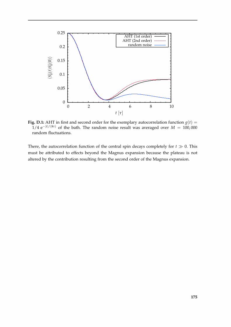
0
0.05
0.1
0.15
0.2
0.25
0 2 4 6 8 10
〈Sz 0(
t)S
z 0(0)〉
t [τ]
AHT (1st order)AHT (2nd order)
random noise
Fig. D.1: AHT in first and second order for the exemplary autocorrelation function g(t) =1/4 e−|t|/(8τ) of the bath. The random noise result was averaged over M = 100, 000random fluctuations.
There, the autocorrelation function of the central spin decays completely for t ≫ 0. This
must be attributed to effects beyond the Magnus expansion because the plateau is not
altered by the contribution resulting from the second order of the Magnus expansion.
175

Appendix E
Sampling of Random Gaussian Fluctuations
The ability to sample random Gaussian noise η(t) obeying a pre-defined autocorrelation
function
g (t1 − t2) = η (t1) η (t2)
= η (t1 − t2))η (0)(E.1a)
is required for the numerical investigation of the semiclassical models in Chapters 3 and
5. We assume that the mean value
η (t) = 0 (E.1b)
vanishes since it would only induce a constant offset.
In this appendix, we explain how the noise can be generated for arbitrary autocorrelation
functions g(t). The only requirement is the capability of sampling white Gaussian noise
h(t) with properties
h (t1) h (t2) = h0δ (t1 − t2) (E.2a)
h (t) = 0. (E.2b)
The underlying white noise h(t) has to be Gaussian because we want that the sampled
fluctuations η(t) are Gaussian as well. They are both linked via linear transformations
so that the Gaussian character of the noise is conserved. As we are dealing with a very
large number of fluctuations, the employed random number generator must have a very
large period. A well-established and reliable generator is the Mersenne Twister generator
which passes many statistical tests [MN98]. Its implementation is part of several numerical
libraries such as the GNU Scientific Library (GSL) [GDT+09]. The library also includes the
Box-Muller transformation which generates random numbers obeying a Gaussian distri-
bution from the output of the random number generator.
177
Appendix E Sampling of Random Gaussian Fluctuations
E.1 Exponentially decaying autocorrelation functions
For the beginning, we restrict ourselves to Gaussian noise η(t) with exponentially decaying
autocorrelation function
g (t) = g20 e−γ|t| (E.3a)
η (t) = 0. (E.3b)
The exponential shape of the autocorrelation function resembles the one of processes sum-
marized under the name Ornstein-Uhlenbeck process [UO30].
The noise η(t) can be viewed as fulfilling the inhomogeneous linear differential equation
η = −γη + h (t) , (E.4)
where h(t) represents the white noise. The general solution to Eq. (E.4) is given by
η (t) =
t∫
0
dt′ h(t′) eγt′ +η0
e−γt, (E.5)
with η0 := η(0). It is derived from the solution of the homogeneous differential equation
involving a variation of parameters. For determining the appropriate values of h0 and η0,
we calculate the autocorrelation function
η (t1) η (t2)h= e−γ(t1+t2)
η2
0 + η0
t1∫
0
dt′1 h(t′1) eγt′1 +
t2∫
0
dt′2 h(t′2) eγt′2
+
t1∫
0
dt′1
t2∫
0
dt′2 h(t′1)h(t′2) eγ(t′1+t′2)
h
,
(E.6a)
where the average is carried out with respect to the white Gaussian noise h(t). By exploit-
ing its properties (E.2a), the latter expression simplifies to
g(t1, t2) = e−γ(t1+t2)
η2
0 + h0
t1∫
0
dt′1
t2∫
0
dt′2 δ (t1 − t2) eγ(t′1+t′2)
. (E.6b)
Without loss of generality, we may assume 0 < t2 < t1 and obtain
g(t1, t2) = η20 e−γ(t1+t2)+
h0
2γ
(e−γ(t1−t2) − e−γ(t1+t2)
)(E.6c)
178
E.2 Arbitrary autocorrelation functions
for the preliminary result of the autocorrelation function. The latter expression does not
solely depend on the relative time t1 − t2 which is unphysical. It acquires the desired
form (E.3a) if the intrinsic parameter h0 corresponding to the variance of the white Gaus-
sian noise is chosen to be
h0 = 2γg20 (E.7)
with g20 ≡ η2
0 . Thereby, we have shown that the Gaussian fluctuations sampled via the dif-
ferential equation (E.4) indeed have an exponentially decaying autocorrelation function.
In the numerics, one deals with a discretized time axis t → ti = i∆t with ∆t being an
appropriate small time interval. The continuous fluctuation η(t) is then approximated by
a series η(t) → η(ti) which is sampled from a series of white Gaussian noise h(ti). Its
variance Var h is given as
Var h =h0
∆t, (E.8)
because δ(∆t(i − j)) = δ(i − j)/∆t. After inserting the differential quotient, one obtains the
discretized form of the differential equation (E.4)
η(ti+1) = ∆t(−γη(ti) + h(ti)
)+ η(ti). (E.9)
The initial value η0 of the fluctuations is chosen randomly from white Gaussian noise with
vanishing mean value η0 = 0 and variance Var η0 = g20.
As an example, the autocorrelation function g(t) and the mean value η(t) is plotted in
Fig. E.1 for γ = g0. For the numerical evaluation, the energy scale is again set to g0 = 1.
Already for a moderate number M of sampled fluctuations, the autocorrelation function
g(t) is in very nice agreement with the exact one. The mean value fluctuates within in the
error bars which are ∼ 1/√
M.
E.2 Arbitrary autocorrelation functions
In the following, we present a simple approach for sampling fluctuations obeying an ar-
bitrary autocorrelation function g(t). The autocorrelation function may be represented by
an analytical function or by numerical data, for example from a DMRG calculation.
We assume a t-axis which is discretized into D intervals. The fluctuations η(ti) have
179
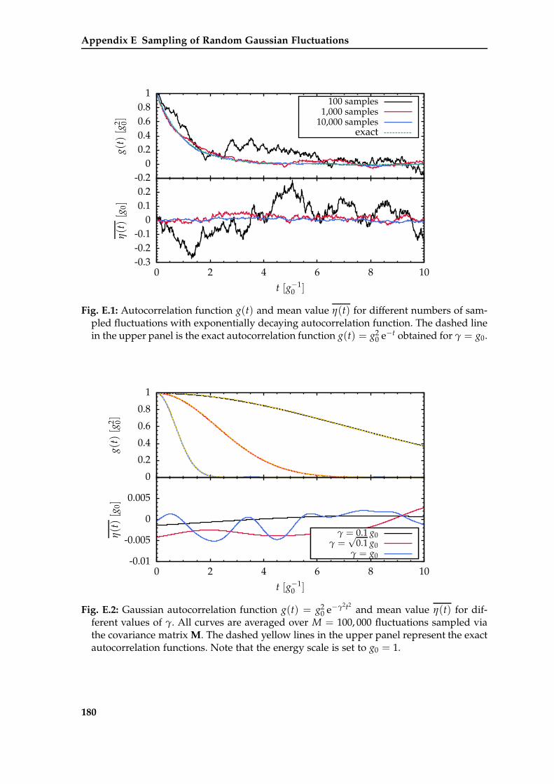
Appendix E Sampling of Random Gaussian Fluctuations
-0.20
0.20.40.60.8
1
g(t)[g
2 0]
-0.3-0.2-0.1
00.10.2
0 2 4 6 8 10
η(t)[g
0]
t [g−10 ]
100 samples1,000 samples
10,000 samplesexact
Fig. E.1: Autocorrelation function g(t) and mean value η(t) for different numbers of sam-pled fluctuations with exponentially decaying autocorrelation function. The dashed linein the upper panel is the exact autocorrelation function g(t) = g2
0 e−t obtained for γ = g0.
0
0.2
0.4
0.6
0.8
1
g(t)[g
2 0]
-0.01
-0.005
0
0.005
0 2 4 6 8 10
η(t)[g
0]
t [g−10 ]
γ = 0.1 g0γ =
√0.1 g0
γ = g0
Fig. E.2: Gaussian autocorrelation function g(t) = g20 e−γ2t2
and mean value η(t) for dif-ferent values of γ. All curves are averaged over M = 100, 000 fluctuations sampled viathe covariance matrix M. The dashed yellow lines in the upper panel represent the exactautocorrelation functions. Note that the energy scale is set to g0 = 1.
180
E.2 Arbitrary autocorrelation functions
to fulfill a Gaussian distribution at every discrete time step ti. This can be interpreted as
D-dimensional Gaussian distribution
p(~η)=
1
(2π)D/2 √det Me−
12~η
⊤M−1~η (E.10)
where the D-dimensional vector ~η = (η(t1) . . . η(tD))⊤ contains the discretized fluctua-
tions, see Appendix D for comparison. In multiple dimensions, the covariance matrix M
replaces the variance. Hence, it holds the values of the autocorrelation function as entries
Mij := g(ti − tj). (E.11)
It follows directly from the properties of the autocorrelation function that M is a symmetric
matrix. Thus, it is diagonalizable
D = O⊤MO (E.12)
via an orthogonal transformation O containing the eigenvectors ~λi of M as columns. The
relation
~η′ = O⊤~η (E.13)
transforms the vector ~η to the vector ~η′ in the diagonal basis. Due to this linear transforma-
tion, the vector ~η′ fulfills a Gaussian probability distribution characterized by the diagonal
covariance matrix D. It contains the eigenvalues λi ≥ 0 of M on its main diagonal. By
definition, all eigenvalues λi have to be positive because they correspond to the variance
of the fluctuations in the diagonal basis. Consequently, the non-diagonal matrix M is pos-
itive semi-definite. But in practice this property may be violated due to rounding errors,
see below.
Thereby, we have all ingredients for sampling the fluctuations ~η. The procedure reads as
follows:
1) Construct the covariance matrix M according to Eq. (E.11).
2) Diagonalize M to obtain all eigenvalues λi and -vectors ~λi forming the columns of
the transformation O.
3) Sample the fluctuations ~η′ = (η′(t1) . . . η′(tD))⊤ in the diagonal basis according to
a Gaussian probability distribution with variance
Var η′(ti) = λi (E.14)
181
Appendix E Sampling of Random Gaussian Fluctuations
and vanishing mean value.
4) Transform the fluctuations back to the non-diagonal basis via
~η = O~η′. (E.15)
The fluctuations sampled via this algorithm satisfy the autocorrelation function g(t) which
entered in the construction of the covariance matrix M. This principle can easily be ex-
tended to autocorrelation functions spanning all spatial dimensions x, y, and z. Then, the
covariance matrix is a 3 × 3 block matrix
M =
Mxx Mxy Mxz
Myx Myy Myz
Mzx Mzy Mzz
(E.16a)
formed by the individual D × D covariance matrices Mαβ = (Mαβij ) with entries
Mαβij = gαβ(ti − tj), α, β ∈ x, y, z. (E.16b)
If an external field is applied in one direction, the covariance matrix has block diagonal
form because there is no correlation between the spin directions parallel and perpendicular
to the external field.
Problems may arise in step 3) of the algorithm where the square root of the eigenvalues
λi has to be calculated. By definition, a covariance matrix is positive semi-definite. But in
practice negative eigenvalues may occur due to the discretization and numerical inaccura-
cies. This is a widely known problem in fields where covariance matrices are constructed
from empirical data, for example in finance. Mathematical algorithms have been devel-
oped to find the nearest positive semi-definite covariance matrix to a given matrix [Hig02].
In our applications, only very small negative eigenvalues occur stemming from rounding
errors and a numerical correction of the covariance matrix is not necessary. For the sampled
fluctuations with Gaussian autocorrelation function shown in Fig. E.2, the largest negative
eigenvalues still lie below −10−12. They may simply be set to zero without any negative
effect on the results. From our practical experience, this procedure can be carried out even
for larger negative eigenvalues as long as |λi| . 10−6-10−5.
182
Appendix F
Piecewise Constant Pulses
In this appendix, the details of the π-pulses studied in Chapter 5 are summarized. All
pulses consist of piecewise constant amplitudes and rotate the spin either around the x- or
around the y-axis. Hence, they only prevent the dephasing of the electron spin. The investi-
gated pulses comprise the well-known symmetric SCORPSE and the asymmetric CORPSE
pulse [CJ00, CLJ03] which are both first order pulses. Furthermore, a second order pulse
derived for a classical bath [Sti12, SFPU12] is studied. In addition, we discuss the second
order symmetric SYM2ND and the asymmetric ASYM2ND pulses from Ref. [PKRU09]
where the bath was treated on the quantum level.
The time dependence of the pulse amplitudes v(t) is plotted in Fig. F.1, while the corre-
sponding switching instances τi and amplitudes vτiare listed in Tab. F.1.
The parameters of the second order pulses in Tab. F.1 are given in the same high precision
as used in our numerical simulation. Thereby, a substantial increase of the accuracy is
gained compared to the low-precision parameters published in Refs. [PKRU09, SFPU12].
The author is indebted to S. Pasini for providing the high-precision parameters of the
SYM2ND and ASYM2ND pulse [Pas13] and to C. Stihl for providing the high-precision
parameters of the second order pulse optimized for a classical bath [Sti13].
183
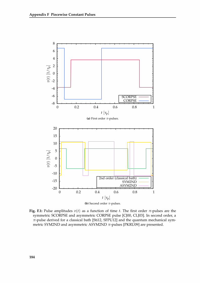
Appendix F Piecewise Constant Pulses
-8
-6
-4
-2
0
2
4
6
8
0 0.2 0.4 0.6 0.8 1
v(t)[1
/τ p]
t [τp]
SCORPSECORPSE
(a) First order π-pulses.
-20
-15
-10
-5
0
5
10
15
20
0 0.2 0.4 0.6 0.8 1
v(t)[1
/τ p]
t [τp]
2nd order (classical bath)SYM2ND
ASYM2ND
(b) Second order π-pulses.
Fig. F.1: Pulse amplitudes v(t) as a function of time t. The first order π-pulses are thesymmetric SCORPSE and asymmetric CORPSE pulse [CJ00, CLJ03]. In second order, aπ-pulse derived for a classical bath [Sti12, SFPU12] and the quantum mechanical sym-metric SYM2ND and asymmetric ASYM2ND π-pulses [PKRU09] are presented.
184
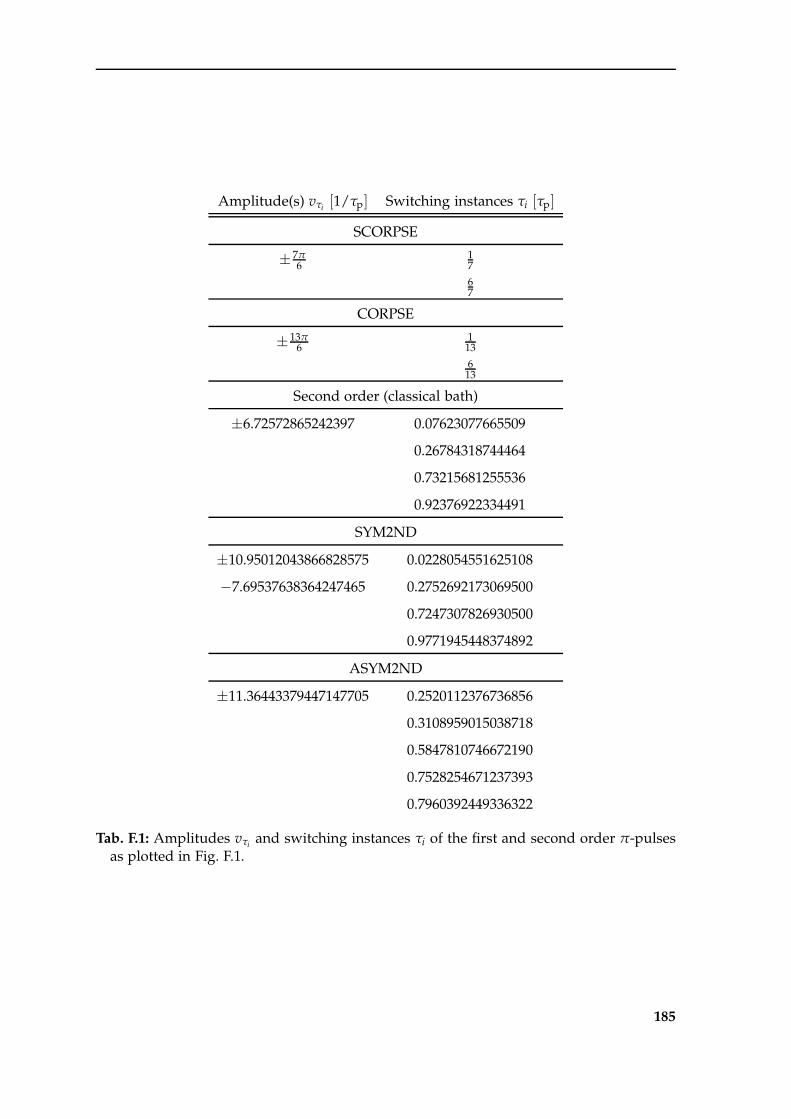
Amplitude(s) vτi[1/τp] Switching instances τi [τp]
SCORPSE
± 7π6
17
67
CORPSE
± 13π6
113
613
Second order (classical bath)
±6.72572865242397 0.07623077665509
0.26784318744464
0.73215681255536
0.92376922334491
SYM2ND
±10.95012043866828575 0.0228054551625108
−7.69537638364247465 0.2752692173069500
0.7247307826930500
0.9771945448374892
ASYM2ND
±11.36443379447147705 0.2520112376736856
0.3108959015038718
0.5847810746672190
0.7528254671237393
0.7960392449336322
Tab. F.1: Amplitudes vτiand switching instances τi of the first and second order π-pulses
as plotted in Fig. F.1.
185

Appendix G
No-Go Theorem for Pulses under Cusp-Like
Autocorrelation Functions
If the correlation function of the random noise exhibits a cusp at t = 0, unexpected half-
integer contributions ∆F ∼ 1/v3/2 arise in the Frobenius norm ∆F. This has to be accounted
to an additional condition emerging for shaped pulses under an Ornstein-Uhlenbeck type
noise of the bath. The supplemental integral is not fulfilled by standard and new pulses
respecting the extended set of conditions have to be derived. However, it can be shown
that both the two standard first order conditions from Eqs. (5.26) as well the supplemental
condition from Eq. (5.28) cannot be fulfilled simultaneously. In the following, we depict an
analytic argument by G. Uhrig which proofs this situation [Uhr13].
We recall the supplemental condition from Eq. (5.28). After the application of an additional
theorem, it can be rewritten in the form
I3/2 = Ia3/2 + Ib
3/2 (G.1)
with
Ia3/2 =
τp∫
0
dt1
τp∫
0
dt2 cos ψ1 |t1 − t2| cos ψ2 (G.2a)
Ib3/2 =
τp∫
0
dt1
τp∫
0
dt2 sin ψ1 |t1 − t2| sin ψ2. (G.2b)
For simplicity, we abbreviate ψi := ψ(ti). In the Hilbert space H of integrable functions,
both integrals may be interpreted as an expectation value
Ia3/2 = 〈cos ψ|A| cos ψ〉 (G.3a)
Ib3/2 = 〈sin ψ|A| sin ψ〉 (G.3b)
187
Appendix G No-Go Theorem for Pulses under Cusp-Like Autocorrelation Functions
of the linear operator
A (t1, t2) = |t1 − t2| . (G.4)
It maps the function ϕ(t) ∈ H onto the function ψ(t) by
A : ϕ (t) 7−→ ψ (t) =
τp∫
0
dt′ A(t, t′)ϕ(t′). (G.5)
The expectation value of the operator A should have a well-defined sign. Hence, we at-
tempt to find a relation A ∼ BB† where the operator B is proportional to the square root
of A. An adequate ansatz for B is given by
B : ϕ (t) 7−→ ψ (t) =
τp∫
0
dt′ sgn(t − t′)ϕ(t′). (G.6)
Consequently, the mapping for B2 reads
B2 : ϕ (t) 7−→ χ (t) =
τp∫
0
dt1
τp∫
0
dt2 sgn(t − t1) sgn(t1 − t2)ϕ(t2). (G.7)
The integration with respect to t1 can be carried out analytically. Then, the latter expres-
sions acquires the form
B2 : ϕ (t) 7−→ χ (t) =
τp∫
0
dt2(2 |t − t2| − 1
)ϕ(t2). (G.8)
Thereby, we have found the desired relation between the operators A and B. It is given
by
A =12
(C − B†B
)(G.9)
where we have exploited the antisymmetry B = −B† of the operator B. Furthermore, the
operator
C : ϕ (t) 7−→ ψ (t) =
τp∫
0
dt′ ϕ(t′) (G.10)
has been introduced. Compared to the operators A and B, the mapping of C simply cor-
responds to the identity.
188
Now, we restrict ourselves to integrable functions f (t) from a subspace Hs ⊆ H of the
Hilbert space of integrable functions. We assume that every f (t) ∈ Hs accomplishes
0 ≡τp∫
0
dt f (t) . (G.11)
Hence, f (t) represents all pulses which fulfill the standard conditions of a first order
pulse (5.26). The latter expression implies 〈 f |C| f 〉 ≡ 0. Together with the relation from
Eq. (G.9), we obtain the expression
〈 f |A| f 〉 = −12〈B f |B f 〉 ≤ 0 (G.12)
for the expectation value of the operator A. It is valid for all f (t) ∈ Hs and explains why
the supplemental integral I3/2 from Eq. (5.27) never changes its sign.
However, we still have to verify whether f (t) can make Eq. (G.12) in addition to Eq. (G.11)
vanish. This implies
0 ≡ B | f 〉
⇔ 0 ≡ ψ (t) =
τp∫
0
dt′ sgn(t − t′) f (t′)(G.13)
for all values of t. The latter expression is differentiated with respect to t, which yields
∂t ψ (t) = 2
τp∫
0
dt′ δ(t − t′) f (t′)
= 2 f (t) 6= 0.
(G.14)
This expression stands in contradiction to Eq. (G.13) because the derivative ∂t ψ(t) should
be equivalent to zero when ψ(t) ≡ 0. Hence, the strict inequality in Eq. (G.12) always
holds for all f (t) ∈ Hs. Thereby, we have proven rigorously that a shaped pulse cannot
accomplish the standard conditions from Eqs. (5.26) and the supplemental condition from
Eq. (5.28) simultaneously. As a consequence, pulses designed for an Ornstein-Uhlenbeck
type noise should be optimized in a way that the standard integrals (5.26) vanish under
the constraint that the supplemental integral (5.28) is minimized. Then, the influence of
the half-integer contribution ∆F ∼ 1/v3/2 is diminished.
189

Appendix H
DMRG versus a Non-Perturbative Master Equation
Solution
In the following, we compare the maximum time accessible within our numerical ansatz
based on the DMRG with the limitations of the non-perturbative master equation solution
for the central spin model by Barnes et al. [BCDS12]. To this end, we calculate the limiting
parameters of the latter approach, namely the largest coupling constant and the value
of the finite external magnetic field, for our uniform distribution of couplings defined in
Eq. (1.8) and the parameters given in Ref. [BCDS12].
In contrast to the DMRG, the solution of the master equation always requires a finite
external magnetic field. Moreover, its validity is limited to the time scale set by the largest
coupling constant
tmax =1
Jmax. (H.1)
The results in Ref. [BCDS12] are characterized by the quantity
Λ :=Jtot
h0, (H.2)
where
Jtot =N
∑i=1
Ji (H.3a)
is the total interaction energy and
h0 = gµBB (H.3b)
191
Appendix H DMRG versus a Non-Perturbative Master Equation Solution
is the Zeeman energy. Here, g = 2 is the g-factor of the electron spin and µB = 57.88 µeV/T
is the Bohr magneton. For the specified external magnetic field of strength B = 100 mT
and Λ = 30 [BCDS12], the quantities in Eqs. (H.3) acquire the values Jtot = 347.28 µeV and
h0 = 11.58 µeV, respectively.
With Jmax ≡ J1 and our distribution for the Ji defined in Eq. (1.8), the maximum time tmax
in units of J−1q can directly be deduced from Eq. (H.1) in dependence of the bath size N.
Furthermore, the absolute value of Jq in µeV has to be calculated. For this, we evaluate the
quantity
Jtot
Jq=
√6N
2N2 + 3N + 1N + 1
2. (H.4)
for a fixed N. Subsequently, one obtains the corresponding value of Jq in µeV by dividing
the absolute value Jtot = 347.28 µeV through the result of Eq. (H.4). Finally, we are able to
express the parameter h0 in units of Jq to determine the regime of the magnetic field in
which the non-perturbative master equation solution is valid.
All extracted parameters are summarized in Tab. H.1 for exemplary numbers of N. The
limiting time tmax of the non-perturbative master equation solution has to be compared
with the maximum time tDMRGmax of the DMRG calculation for the corresponding values of
N and h0. Note, however, that there is no well-defined tDMRGmax . Hence, the values in Tab. H.1
are based on our experience.
For all values of N, our ansatz based on the DMRG outperforms the non-perturbative
master equation solution. We stress that the parameter h0/Jq increases with N because
Jtot ∼√
N. This observation is crucial because the solution of the master equation was
obtained in the large-bath limit [BCDS12]. For large baths, the quantity h0/Jq has to take
a substantial value to compensate the decreasing energy scale Jq. Consequently, one ar-
rives quickly in the strong-field regime where the DMRG works extremely well and the
dynamics is essentially classical. In addition, we highlight once more that the investigation
of the zero-field limited on the basis of the non-perturbative master equation solution is
excluded rigorously.
192
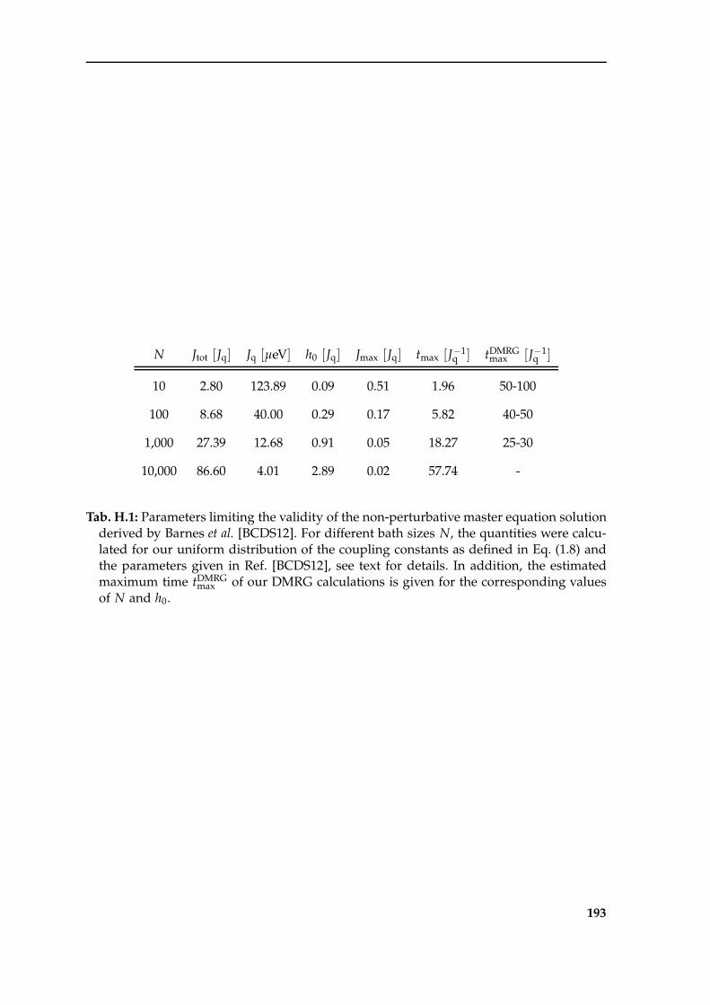
N Jtot [Jq] Jq [µeV] h0 [Jq] Jmax [Jq] tmax [J−1q ] tDMRG
max [J−1q ]
10 2.80 123.89 0.09 0.51 1.96 50-100
100 8.68 40.00 0.29 0.17 5.82 40-50
1,000 27.39 12.68 0.91 0.05 18.27 25-30
10,000 86.60 4.01 2.89 0.02 57.74 -
Tab. H.1: Parameters limiting the validity of the non-perturbative master equation solutionderived by Barnes et al. [BCDS12]. For different bath sizes N, the quantities were calcu-lated for our uniform distribution of the coupling constants as defined in Eq. (1.8) andthe parameters given in Ref. [BCDS12], see text for details. In addition, the estimatedmaximum time tDMRG
max of our DMRG calculations is given for the corresponding valuesof N and h0.
193

Bibliography
[AF11] Alvermann, A. and Fehske, H. High-order commutator-free exponential
time-propagation of driven quantum systems. J. Comput. Phys. 230 (15), 5930
(2011).
[AFL12] Alvermann, A., Fehske, H., and Littlewood, P. B. Numerical time propa-
gation of quantum systems in radiation fields. New J. Phys. 14 (10), 105008
(2012).
[AHDDH06] Al-Hassanieh, K., Dobrovitski, V., Dagotto, E., and Harmon, B. N. Nu-
merical modeling of the central spin problem using the spin-coherent-state
P representation. Phys. Rev. Lett. 97 (3), 037204 (2006).
[Ban98] Ban, M. Photon-echo technique for reducing the decoherence of a quantum
bit. J. Mod. Opt. 45 (11), 2315 (1998).
[BB11] Biercuk, M. J. and Bluhm, H. Phenomenological study of decoherence in
solid-state spin qubits due to nuclear spin diffusion. Phys. Rev. B 83 (23),
235316 (2011).
[BBP04] Breuer, H.-P., Burgarth, D., and Petruccione, F. Non-markovian dynam-
ics in a spin star system: Exact solution and approximation techniques. Phys.
Rev. B 70 (4), 045323 (2004).
[BCDS12] Barnes, E., Cywinski, L., and Das Sarma, S. Nonperturbative master equa-
tion solution of central spin dephasing dynamics. Phys. Rev. Lett. 109 (14),
140403 (2012).
[BCOR09] Blanes, S., Casas, F., Oteo, J., and Ros, J. The magnus expansion and some
of its applications. Phys. Rep. 470 (5-6), 151 (2009).
195
Bibliography
[BCP08] Bulla, R., Costi, T. A., and Pruschke, T. Numerical renormalization group
method for quantum impurity systems. Rev. Mod. Phys. 80 (2), 395 (2008).
[BES+10a] Bortz, M., Eggert, S., Schneider, C., Stübner, R., and Stolze, J. Dynamics
and decoherence in the central spin model using exact methods. Phys. Rev.
B 82 (16), 161308 (2010).
[BES10b] Bortz, M., Eggert, S., and Stolze, J. Spectrum and screening cloud in the
central spin model. Phys. Rev. B 81 (3), 035315 (2010).
[BEU00] Bühler, A., Elstner, N., and Uhrig, G. High temperature expansion for
frustrated and unfrustrated S = 1/2 spin chains. Eur. Phys. J. B 16 (3), 475
(2000).
[BHH+01] Bayer, M., Hawrylak, P., Hinzer, K., Fafard, S., Korkusinski, M.,
Wasilewski, Z. R., Stern, O., and Forchel, A. Coupling and entangling of
quantum states in quantum dot molecules. Science 291 (5503), 451 (2001).
[Bor07] Bortz, M. Private communication (2007).
[BP07] Breuer, H.-P. and Petruccione, F. The Theory of Open Quantum Systems.
Oxford University Press, Oxford, paperback edition (2007).
[BPG+10] Barmettler, P., Punk, M., Gritsev, V., Demler, E., and Altman, E. Quan-
tum quenches in the anisotropic spin-1/2 Heisenberg chain: Different ap-
proaches to many-body dynamics far from equilibrium. New J. Phys. 12 (5),
055017 (2010).
[BS07a] Bortz, M. and Stolze, J. Exact dynamics in the inhomogeneous central-spin
model. Phys. Rev. B 76 (1), 014304 (2007).
[BS07b] Bortz, M. and Stolze, J. Spin and entanglement dynamics in the central-
spin model with homogeneous couplings. J. Stat. Mech. 2007 (6), P06018
(2007).
[BS11] Bortz, M. and Stolze, J. Private communication (2011).
[BSW09] Barthel, T., Schollwöck, U., and White, S. R. Spectral functions in one-
196
Bibliography
dimensional quantum systems at finite temperature using the density ma-
trix renormalization group. Phys. Rev. B 79 (24), 245101 (2009).
[CBB07] Chen, G., Bergman, D. L., and Balents, L. Semiclassical dynamics and
long-time asymptotics of the central-spin problem in a quantum dot. Phys.
Rev. B 76 (4), 045312 (2007).
[CDDS10] Cywinski, L., Dobrovitski, V. V., and Das Sarma, S. Spin echo decay at
low magnetic fields in a nuclear spin bath. Phys. Rev. B 82 (3), 035315 (2010).
[CHHC06] Cappellaro, P., Hodges, J. S., Havel, T. F., and Cory, D. G. Principles
of control for decoherence-free subsystems. J. Chem. Phys. 125 (4), 044514
(2006).
[CJ00] Cummins, H. K. and Jones, J. A. Use of composite rotations to correct
systematic errors in NMR quantum computation. New J. Phys. 2 (1), 6 (2000).
[CL04] Coish, W. A. and Loss, D. Hyperfine interaction in a quantum dot: Non-
Markovian electron spin dynamics. Phys. Rev. B 70 (19), 195340 (2004).
[CL06] Coish, W. A. and Loss, D. Quantum computing with spins in solids. arXiv
e-print (2006). arXiv:cond-mat/0606550.
[CLJ03] Cummins, H. K., Llewellyn, G., and Jones, J. A. Tackling systematic errors
in quantum logic gates with composite rotations. Phys. Rev. A 67 (4), 042308
(2003).
[CLNDS08] Cywinski, L., Lutchyn, R. M., Nave, C. P., and Das Sarma, S. How to
enhance dephasing time in superconducting qubits. Phys. Rev. B 77 (17),
174509 (2008).
[CLYA07] Coish, W. A., Loss, D., Yuzbashyan, E. A., and Altshuler, B. L. Quantum
versus classical hyperfine-induced dynamics in a quantum dot. J. Appl. Phys.
101 (8), 081715 (2007).
[CP54] Carr, H. Y. and Purcell, E. M. Effects of diffusion on free precession in
nuclear magnetic resonance experiments. Phys. Rev. 94 (3), 630 (1954).
197
Bibliography
[DDR03] Dobrovitski, V. V. and De Raedt, H. A. Efficient scheme for numerical
simulations of the spin-bath decoherence. Phys. Rev. E 67 (5), 056702 (2003).
[DH06] Deng, C. and Hu, X. Analytical solution of electron spin decoherence
through hyperfine interaction in a quantum dot. Phys. Rev. B 73 (24), 241303
(2006).
[DH08] Deng, C. and Hu, X. Electron-spin dephasing via hyperfine interaction in
a quantum dot: An equation-of-motion calculation of electron-spin correla-
tion functions. Phys. Rev. B 78 (24), 245301 (2008).
[DiV00] DiVincenzo, D. P. The physical implementation of quantum computation.
Fortschr. Phys. 48 (9-11), 771 (2000).
[DKSV04] Daley, A. J., Kollath, C., Schollwöck, U., and Vidal, G. Time-
dependent density-matrix renormalization-group using adaptive effective
Hilbert spaces. J. Stat. Mech. 2004 (4), P04005 (2004).
[dLWR+10] de Lange, G., Wang, Z. H., Ristè, D., Dobrovitski, V. V., and Hanson,
R. Universal dynamical decoupling of a single solid-state spin from a spin
bath. Science 330 (1), 60 (2010).
[DMK03] Das, R., Mahesh, T., and Kumar, A. Experimental implementation of
Grover’s search algorithm using efficient quantum state tomography. Chem.
Phys. Lett. 369 (1), 8 (2003).
[DPS04] Dukelsky, J., Pittel, S., and Sierra, G. Colloquium: Exactly solvable
Richardson-Gaudin models for many-body quantum systems. Rev. Mod.
Phys. 76 (3), 643 (2004).
[DRZ+09] Du, J., Rong, X., Zhao, N., Wang, Y., Yang, J., and Liu, R. B. Preserving
electron spin coherence in solids by optimal dynamical decoupling. Nature
461 (7268), 1265 (2009).
[dSDS03a] de Sousa, R. and Das Sarma, S. Electron spin coherence in semiconductors:
Considerations for a spin-based solid-state quantum computer architecture.
Phys. Rev. B 67 (3), 033301 (2003).
[dSDS03b] de Sousa, R. and Das Sarma, S. Theory of nuclear-induced spectral dif-
198
Bibliography
fusion: Spin decoherence of phosphorus donors in Si and GaAs quantum
dots. Phys. Rev. B 68 (11), 115322 (2003).
[EHWvB+04] Elzerman, J. M., Hanson, R., Willems van Beveren, L. H., Witkamp, B.,
Vandersypen, L. M. K., and Kouwenhoven, L. P. Single-shot read-out of
an individual electron spin in a quantum dot. Nature 430 (6998), 431 (2004).
[EN02] Erlingsson, S. I. and Nazarov, Y. V. Hyperfine-mediated transitions be-
tween a Zeeman split doublet in GaAs quantum dots: The role of the inter-
nal field. Phys. Rev. B 66 (15), 155327 (2002).
[EN04] Erlingsson, S. I. and Nazarov, Y. V. Evolution of localized electron spin in
a nuclear spin environment. Phys. Rev. B 70 (20), 205327 (2004).
[Fau13] Fauseweh, B. Private communication (2013).
[FB07] Fischer, J. and Breuer, H.-P. Correlated projection operator approach to
non-Markovian dynamics in spin baths. Phys. Rev. A 76 (5), 052119 (2007).
[FBN+08] Ferraro, E., Breuer, H.-P., Napoli, A., Jivulescu, M. A., and Messina,
A. Non-Markovian dynamics of a single electron spin coupled to a nuclear
spin bath. Phys. Rev. B 78 (6), 064309 (2008).
[Fer30] Fermi, E. Über die magnetischen Momente der Atomkerne. Z. Phys. 60 (5),
320 (1930).
[FPU12] Fauseweh, B., Pasini, S., and Uhrig, G. S. Frequency-modulated pulses for
quantum bits coupled to time-dependent baths. Phys. Rev. A 85 (2), 022310
(2012).
[Fri06] Friedrich, A. Time-Dependent Properties of One-Dimensional Spin-Systems: A
DMRG-Study. Ph.D. thesis, RWTH Aachen (2006).
[FS13a] Faribault, A. and Schuricht, D. Integrability-based analysis of the
hyperfine-interaction-induced decoherence in quantum dots. Phys. Rev. Lett.
110 (4), 040405 (2013).
[FS13b] Faribault, A. and Schuricht, D. Spin decoherence due to a randomly
fluctuating spin bath. Phys. Rev. B 88 (8), 085323 (2013).
199
Bibliography
[FTP+05] Facchi, P., Tasaki, S., Pascazio, S., Nakazato, H., Tokuse, A., and Lidar,
D. A. Control of decoherence: Analysis and comparison of three different
strategies. Phys. Rev. A 71 (2), 022302 (2005).
[FW05] Feiguin, A. E. and White, S. R. Time-step targeting methods for real-time
dynamics using the density matrix renormalization group. Phys. Rev. B
72 (2), 020404 (2005).
[Gai01] Gaite, J. Angular quantization and the density matrix renormalization
group. Mod. Phys. Lett. A 16 (17), 1109 (2001).
[Gai03] Gaite, J. Entanglement entropy and the density matrix renormalization
group. arXiv e-print (2003). arXiv:quant-ph/0301120.
[Gau76] Gaudin, M. Diagonalisation d’une classe d’Hamiltoniens de spin. J. Phys.
France 37 (10), 1087 (1976).
[Gau83] Gaudin, M. La Fonction d’Onde de Bethe. Masson, Paris (1983).
[GDT+09] Galassi, M., Davies, J., Theiler, J., Gough, B., Jungman, G., Alken, P.,
Booth, M., and Rossi, F. GNU Scientific Library Reference Manual. Network
Theory Limited, third edition (2009). http://www.gnu.org/software/gsl/.
[GES+09] Greilich, A., Economou, S. E., Spatzek, S., Yakovlev, D. R., Reuter, D.,
Wieck, A. D., Reinecke, T. L., and Bayer, M. Ultrafast optical rotations of
electron spins in quantum dots. Nature Phys. 5 (4), 262 (2009).
[GKL04] Golovach, V. N., Khaetskii, A. A., and Loss, D. Phonon-induced decay of
the electron spin in quantum dots. Phys. Rev. Lett. 93 (1), 016601 (2004).
[GKSS05] Gobert, D., Kollath, C., Schollwöck, U., and Schütz, G. Real-time dy-
namics in spin-1/2 chains with adaptive time-dependent density matrix
renormalization group. Phys. Rev. E 71 (3), 036102 (2005).
[GMD02] Galindo, A. and Martín-Delgado, M. A. Information and computation:
Classical and quantum aspects. Rev. Mod. Phys. 74 (2), 347 (2002).
[Gro96] Grover, L. K. A fast quantum mechanical algorithm for database search. In
200
Bibliography
Proceedings of the twenty-eighth annual ACM symposium on Theory of Comput-
ing, STOC ’96, pages 212–219. ACM, New York, NY, USA (1996).
[Gro97] Grover, L. K. Quantum mechanics helps in searching for a needle in a
haystack. Phys. Rev. Lett. 79 (2), 325 (1997).
[GYS+06] Greilich, A., Yakovlev, D. R., Shabaev, A., Efros, A. L., Yugova, I. A.,
Oulton, R., Stavarache, V., Reuter, D., Wieck, A., and Bayer, M. Mode
locking of electron spin coherences in singly charged quantum dots. Science
313 (5785), 341 (2006).
[HA14] Hackmann, J. and Anders, F. B. Spin noise in the anisotropic central spin
model. Phys. Rev. B 89 (4), 045317 (2014).
[Hac13] Hackmann, J. Private communication (2013).
[Hae76] Haeberlen, U. High Resolution NMR in Solids: Selective Averaging. Advances
in magnetic resonance: Supplement 1. Academic Press, New York, first edi-
tion (1976).
[Hah50] Hahn, E. L. Spin echoes. Phys. Rev. 80 (4), 580 (1950).
[HGB+08] Hernandez, F. G. G., Greilich, A., Brito, F., Wiemann, M., Yakovlev,
D. R., Reuter, D., Wieck, A. D., and Bayer, M. Temperature-induced spin-
coherence dissipation in quantum dots. Phys. Rev. B 78 (4), 041303 (2008).
[Hig02] Higham, N. J. Computing the nearest correlation matrix - a problem from
finance. IMA J. Numer. Anal. 22 (3), 329 (2002).
[HKP+07] Hanson, R., Kouwenhoven, L. P., Petta, J. R., Tarucha, S., and Vander-
sypen, L. M. K. Spins in few-electron quantum dots. Rev. Mod. Phys. 79 (4),
1217 (2007).
[HL97] Hochbruck, M. and Lubich, C. On Krylov subspace approximations to the
matrix exponential operator. SIAM J. Numer. Anal. 34 (5), 1911 (1997).
[HL99] Hochbruck, M. and Lubich, C. Exponential integrators for quantum-
classical molecular dynamics. BIT 39 (4), 620 (1999).
201
Bibliography
[HWM+11] Holzner, A., Weichselbaum, A., McCulloch, I. P., Schollwöck, U., and
von Delft, J. Chebyshev matrix product state approach for spectral func-
tions. Phys. Rev. B 83 (19), 195115 (2011).
[JGP+04] Jelezko, F., Gaebel, T., Popa, I., Domhan, M., Gruber, A., and Wrachtrup,
J. Observation of coherent oscillation of a single nuclear spin and realization
of a two-qubit conditional quantum gate. Phys. Rev. Lett. 93 (13), 130501
(2004).
[Jon11] Jones, J. A. Quantum computing with NMR. Prog. Nucl. Magn. Reson.
Spectrosc. 59 (2), 91 (2011).
[Kan98] Kane, B. E. A silicon-based nuclear spin quantum computer. Nature
393 (6681), 133 (1998).
[KBM12] Karrasch, C., Bardarson, J. H., and Moore, J. E. Finite-temperature dy-
namical density matrix renormalization group and the drude weight of
spin-1/2 chains. Phys. Rev. Lett. 108 (22), 227206 (2012).
[KDH+04] Kroutvar, M., Ducommun, Y., Heiss, D., Bichler, M., Schuh, D., Abstre-
iter, G., and Finley, J. J. Optically programmable electron spin memory
using semiconductor quantum dots. Nature 432 (7013), 81 (2004).
[KL05] Khodjasteh, K. and Lidar, D. A. Fault-tolerant quantum dynamical de-
coupling. Phys. Rev. Lett. 95 (18), 180501 (2005).
[KL07] Khodjasteh, K. and Lidar, D. A. Performance of deterministic dynamical
decoupling schemes: Concatenated and periodic pulse sequences. Phys. Rev.
A 75 (6), 062310 (2007).
[KLG02] Khaetskii, A. V., Loss, D., and Glazman, L. Electron spin decoherence in
quantum dots due to interaction with nuclei. Phys. Rev. Lett. 88 (18), 186802
(2002).
[KLG03] Khaetskii, A., Loss, D., and Glazman, L. Electron spin evolution induced
by interaction with nuclei in a quantum dot. Phys. Rev. B 67 (19), 195329
(2003).
[KMB+08] Kuopanportti, P., Möttönen, M., Bergholm, V., Saira, O.-P., Zhang, J.,
202
Bibliography
and Whaley, K. B. Suppression of 1/ f α noise in one-qubit systems. Phys.
Rev. A 77 (3), 032334 (2008).
[KN00] Khaetskii, A. V. and Nazarov, Y. V. Spin relaxation in semiconductor quan-
tum dots. Phys. Rev. B 61 (19), 12639 (2000).
[KN01] Khaetskii, A. V. and Nazarov, Y. V. Spin-flip transitions between Zee-
man sublevels in semiconductor quantum dots. Phys. Rev. B 64 (12), 125316
(2001).
[KNV08] Koppens, F. H. L., Nowack, K. C., and Vandersypen, L. M. K. Spin echo
of a single electron spin in a quantum dot. Phys. Rev. Lett. 100 (23), 236802
(2008).
[Lan50] Lanczos, C. An iteration method for the solution of the eigenvalue problem
of linear differential and integral operators. J. Res. Natl. Bur. Stand. 45 (4),
255 (1950).
[LBMW03] Leibfried, D., Blatt, R., Monroe, C., and Wineland, D. Quantum dynam-
ics of single trapped ions. Rev. Mod. Phys. 75 (1), 281 (2003).
[LD98] Loss, D. and DiVincenzo, D. P. Quantum computation with quantum dots.
Phys. Rev. A 57 (1), 120 (1998).
[Lev08] Levitt, M. H. Spin Dynamics: Basics of Nuclear Magnetic Resonance. John
Wiley & Sons Ltd., Chichester, second edition (2008).
[LJL+10] Ladd, T. D., Jelezko, F., Laflamme, R., Nakamura, Y., Monroe, C., and
O’Brien, J. L. Quantum computers. Nature 464 (7285), 45 (2010).
[LRV04] Latorre, J. I., Rico, E., and Vidal, G. Ground state entanglement in quan-
tum spin chains. Quant. Inf. Comput. 4 (1), 48 (2004).
[LYS10] Liu, R.-B., Yao, W., and Sham, L. Quantum computing by optical control of
electron spins. Adv. Phys. 59 (5), 703 (2010).
[Mag54] Magnus, W. On the exponential solution of differential equations for a
linear operator. Comm. Pure Appl. Math. 7 (4), 649 (1954).
203
Bibliography
[MdSZW06] Möttönen, M., de Sousa, R., Zhang, J., and Whaley, K. B. High-fidelity
one-qubit operations under random telegraph noise. Phys. Rev. A 73, 022332
(2006).
[MER02] Merkulov, I. A., Efros, A. L., and Rosen, M. Electron spin relaxation by
nuclei in semiconductor quantum dots. Phys. Rev. B 65 (20), 205309 (2002).
[MG58] Meiboom, S. and Gill, D. Modified spin-echo method for measuring nu-
clear relaxation times. Rev. Sci. Instrum. 29 (8), 688 (1958).
[MMN05] Manmana, S. R., Muramatsu, A., and Noack, R. M. Time evolution of
one-dimensional quantum many body systems. AIP Conf. Proc. 789 (1), 269
(2005).
[MN98] Matsumoto, M. and Nishimura, T. Mersenne Twister: A 623-dimensionally
equidistributed uniform pseudo-random number generator. ACM Trans.
Model. Comput. Simul. 8 (1), 3 (1998).
[MSS01] Makhlin, Y., Schön, G., and Shnirman, A. Quantum-state engineering
with Josephson-junction devices. Rev. Mod. Phys. 73 (2), 357 (2001).
[MTA+06] Morton, J. J. L., Tyryshkin, A. M., Ardavan, A., Benjamin, S. C.,
Porfyrakis, K., Lyon, S. A., and Briggs, G. A. D. Bang-bang control of
fullerene qubits using ultrafast phase gates. Nature Phys. 2 (1), 40 (2006).
[MTL08] Maze, J. R., Taylor, J. M., and Lukin, M. D. Electron spin decoherence
of single nitrogen-vacancy defects in diamond. Phys. Rev. B 78 (9), 094303
(2008).
[NC10] Nielsen, M. A. and Chuang, I. L. Quantum Computation and Quantum Infor-
mation. Cambridge University Press, Cambridge, tenth anniversary edition
(2010).
[NM05] Noack, R. M. and Manmana, S. R. Diagonalization- and numerical
renormalization-group-based methods for interacting quantum systems.
AIP Conf. Proc. 789 (1), 93 (2005).
[ON02] Osborne, T. J. and Nielsen, M. A. Entanglement, quantum phase transi-
204
Bibliography
tions, and density matrix renormalization. Quantum Inf. Process. 1 (1-2), 45
(2002).
[Pas13] Pasini, S. Private communication (2013).
[PFKU08] Pasini, S., Fischer, T., Karbach, P., and Uhrig, G. S. Optimization of short
coherent control pulses. Phys. Rev. A 77 (3), 032315 (2008).
[PKRU09] Pasini, S., Karbach, P., Raas, C., and Uhrig, G. S. Optimized pulses for
the perturbative decoupling of a spin and a decoherence bath. Phys. Rev. A
80 (2), 022328 (2009).
[PKU11] Pasini, S., Karbach, P., and Uhrig, G. S. High-order coherent control se-
quences of finite-width pulses. Europhys. Lett. 96 (1), 10003 (2011).
[PKWH99] Peschel, I., Kaulke, M., Wang, X., and Hallberg, K. A. (Editors). Density-
Matrix Renormalization - A New Numerical Method in Physics, volume 528 of
Lecture Notes in Physics. Springer, Berlin, first edition (1999).
[PQ08] Pryadko, L. P. and Quiroz, G. Soft-pulse dynamical decoupling in a cavity.
Phys. Rev. A 77 (1), 012330 (2008).
[Pre98] Preskill, J. Reliable quantum computers. Proc. R. Soc. Lond. A 454 (1969),
385 (1998).
[PS08] Pryadko, L. P. and Sengupta, P. Second-order shaped pulses for solid-state
quantum computation. Phys. Rev. A 78 (3), 032336 (2008).
[PTVF07] Press, W. H., Teukolsky, S. A., Vetterling, W. T., and Flannery, B. P. Nu-
merical Recipes: The Art of Scientific Computing. Cambridge University Press,
Cambridge, third edition (2007).
[PU08] Pasini, S. and Uhrig, G. S. Generalization of short coherent control pulses:
extension to arbitrary rotations. J. Phys. A 41 (31), 312005 (2008).
[Sch07] Schmidt, E. Zur Theorie der linearen und nichtlinearen Integralgleichun-
gen. Math. Ann. 63 (4), 433 (1907).
205
Bibliography
[Sch04] Schmitteckert, P. Nonequilibrium electron transport using the density
matrix renormalization group method. Phys. Rev. B 70 (12), 121302 (2004).
[Sch05a] Schollwöck, U. The density-matrix renormalization group. Rev. Mod. Phys.
77 (1), 259 (2005).
[Sch05b] Schwabl, F. Quantenmechanik. Springer, Berlin, sixth edition (2005).
[Sch08] Schneider, C. Dekohärenzphänomene im anisotropen Gaudin-Modell. Diploma
thesis, Technische Universität Dortmund (2008).
[Sch11] Schollwöck, U. The density-matrix renormalization group in the age of
matrix product states. Ann. Phys. 326 (1), 96 (2011).
[SFPU12] Stihl, C., Fauseweh, B., Pasini, S., and Uhrig, G. S. Modulated pulses com-
pensating classical noise. ArXiv e-prints (2012). arXiv:quant-ph/1210.4311.
[Sho94] Shor, P. Algorithms for quantum computation: Discrete logarithms and
factoring. In 35th Annual Symposium on Foundations of Computer Science, 1994
Proceedings, pages 124–134 (1994).
[Sho97] Shor, P. Polynomial-time algorithms for prime factorization and discrete
logarithms on a quantum computer. SIAM J. Comput. 26 (5), 1484 (1997).
[SKL03] Schliemann, J., Khaetskii, A., and Loss, D. Electron spin dynamics in
quantum dots and related nanostructures due to hyperfine interaction with
nuclei. J. Phys.: Condens. Matter 15 (50), R1809 (2003).
[SKL+06] Skinner, T. E., Kobzar, K., Luy, B., Bendall, M. R., Bermel, W., Khaneja,
N., and Glaser, S. J. Optimal control design of constant amplitude phase-
modulated pulses: Application to calibration-free broadband excitation. J.
Magn. Reson. 179 (2), 241 (2006).
[SMP02] Saykin, S., Mozyrsky, D., and Privman, V. Relaxation of shallow donor
electron spin due to interaction with nuclear spin bath. Nano Lett. 2 (6), 651
(2002).
[SP05] Sengupta, P. and Pryadko, L. P. Scalable design of tailored soft pulses for
coherent control. Phys. Rev. Lett. 95 (3), 037202 (2005).
206
Bibliography
[SR94] Silver, R. and Röder, H. Densities of states of mega-dimensional Hamilto-
nian matrices. Int. J. Mod. Phys. C 5 (04), 735 (1994).
[SRU13] Stanek, D., Raas, C., and Uhrig, G. S. Dynamics and decoherence in the
central spin model in the low-field limit. Phys. Rev. B 88 (15), 155305 (2013).
[SS08] Stolze, J. and Suter, D. Quantum Computing. A Short Course from Theory to
Experiment. Wiley-VCH, Weinheim, second edition (2008).
[Ste96a] Steane, A. Error correcting codes in quantum theory. Phys. Rev. Lett. 77 (5),
793 (1996).
[Ste96b] Steane, A. Multiple-particle interference and quantum error correction.
Proc. R. Soc. Lond. A 452 (1954), 255 (1996).
[Sti12] Stihl, C. Optimierung von Pulsen zur Entkopplung eines Spins von klassischem
Rauschen: Amplituden- und Frequenzmodulation gegen Dephasierung und Deko-
härenz. Diploma thesis, Technische Universität Dortmund (2012).
[Sti13] Stihl, C. Private communication (2013).
[Stü08] Stübner, R. Dekohärenz im inhomogenen Gaudin-Modell. Diploma thesis,
Technische Universität Dortmund (2008).
[Stü12] Stübner, R. Private communication (2012).
[TEK84] Tal-Ezer, H. and Kosloff, R. An accurate and efficient scheme for propa-
gating the time dependent Schrödinger equation. J. Chem. Phys. 81 (9), 3967
(1984).
[Tyc83] Tycko, R. Broadband population inversion. Phys. Rev. Lett. 51 (9), 775 (1983).
[Uhr07] Uhrig, G. S. Keeping a quantum bit alive by optimized π-pulse sequences.
Phys. Rev. Lett. 98 (10), 100504 (2007). Erratum: Phys. Rev. Lett. 106 (12),
129901 (March 2011).
[Uhr09] Uhrig, G. S. Concatenated control sequences based on optimized dynamic
decoupling. Phys. Rev. Lett. 102 (12), 120502 (2009).
207
Bibliography
[Uhr13] Uhrig, G. S. Private communication (2013).
[UO30] Uhlenbeck, G. E. and Ornstein, L. S. On the theory of the Brownian
motion. Phys. Rev. 36 (5), 823 (1930).
[VC05] Vandersypen, L. M. K. and Chuang, I. L. NMR techniques for quantum
control and computation. Rev. Mod. Phys. 76 (4), 1037 (2005).
[vDP02] von Delft, J. and Poghossian, R. Algebraic Bethe ansatz for a discrete-state
BCS pairing model. Phys. Rev. B 66 (13), 134502 (2002).
[VL98] Viola, L. and Lloyd, S. Dynamical suppression of decoherence in two-state
quantum systems. Phys. Rev. A 58 (4), 2733 (1998).
[VSB+01] Vandersypen, L. M. K., Steffen, M., Breyta, G., Yannoni, C. S., Sher-
wood, M. H., and Chuang, I. L. Experimental realization of Shor’s quantum
factoring algorithm using nuclear magnetic resonance. Nature 414 (6866),
883 (2001).
[War13] Warburton, R. J. Single spins in self-assembled quantum dots. Nature
Mater. 12 (6), 483 (2013).
[WCCDS12] Witzel, W. M., Carroll, M. S., Cywinski, L., and Das Sarma, S. Quantum
decoherence of the central spin in a sparse system of dipolar coupled spins.
Phys. Rev. B 86 (3), 035452 (2012).
[WDS06] Witzel, W. M. and Das Sarma, S. Quantum theory for electron spin de-
coherence induced by nuclear spin dynamics in semiconductor quantum
computer architectures: Spectral diffusion of localized electron spins in the
nuclear solid-state environment. Phys. Rev. B 74 (3), 035322 (2006).
[WDS07] Witzel, W. M. and Das Sarma, S. Multiple-pulse coherence enhancement
of solid state spin qubits. Phys. Rev. Lett. 98 (7), 077601 (2007).
[WdSDS05] Witzel, W. M., de Sousa, R., and Das Sarma, S. Quantum theory of
spectral-diffusion-induced electron spin decoherence. Phys. Rev. B 72 (16),
161306 (2005).
208
Bibliography
[WF04] White, S. R. and Feiguin, A. E. Real-time evolution using the density matrix
renormalization group. Phys. Rev. Lett. 93 (7), 076401 (2004).
[WFL10] West, J. R., Fong, B. H., and Lidar, D. A. Near-optimal dynamical decou-
pling of a qubit. Phys. Rev. Lett. 104 (13), 130501 (2010).
[Whi92] White, S. R. Density-matrix formulation for quantum renormalization-
groups. Phys. Rev. Lett. 69 (19), 2863 (1992).
[Whi93] White, S. R. Density-matrix algorithms for quantum renormalization-
groups. Phys. Rev. B 48 (14), 10345 (1993).
[Whi96] White, S. R. Spin gaps in a frustrated Heisenberg model for CaV4O9. Phys.
Rev. Lett. 77 (17), 3633 (1996).
[Whi98] White, S. R. Strongly correlated electron systems and the density matrix
renormalization group. Phys. Rep. 301 (1-3), 187 (1998).
[Whi05] White, S. R. Density matrix renormalization group algorithms with a single
center site. Phys. Rev. B 72 (18), 180403 (2005).
[Wil75] Wilson, K. G. The renormalization group: Critical phenomena and the
Kondo problem. Rev. Mod. Phys. 47, 773 (1975).
[WL13] Wang, Z.-Y. and Liu, R.-B. No-go theorems and optimization of dynamical
decoupling against noise with soft cutoff. Phys. Rev. A 87 (4), 042319 (2013).
[WN92] White, S. R. and Noack, R. M. Real-space quantum renormalization
groups. Phys. Rev. Lett. 68 (24), 3487 (1992).
[WWAF06] Weiße, A., Wellein, G., Alvermann, A., and Fehske, H. The kernel poly-
nomial method. Rev. Mod. Phys. 78 (1), 275 (2006).
[WYD13] Witzel, W. M., Young, K., and Das Sarma, S. Converting a real
quantum bath to an effective classical noise. ArXiv e-prints (2013).
arXiv:cond-mat.mes-hall/1307.2597.
[YL08a] Yang, W. and Liu, R.-B. Quantum many-body theory of qubit decoherence
in a finite-size spin bath. Phys. Rev. B 78 (8), 085315 (2008).
209
Bibliography
[YL08b] Yang, W. and Liu, R.-B. Universality of Uhrig Dynamical Decoupling for
suppressing qubit pure dephasing and relaxation. Phys. Rev. Lett. 101 (18),
180403 (2008).
[YL09] Yang, W. and Liu, R.-B. Quantum many-body theory of qubit decoherence
in a finite-size spin bath. II. Ensemble dynamics. Phys. Rev. B 79 (11), 115320
(2009).
[YLS07] Yao, W., Liu, R. B., and Sham, L. J. Restoring coherence lost to a slow
interacting mesoscopic spin bath. Phys. Rev. Lett. 98 (7), 077602 (2007).
[ZDAH+06] Zhang, W., Dobrovitski, V. V., Al-Hassanieh, K. A., Dagotto, E., and
Harmon, B. N. Hyperfine interaction induced decoherence of electron spins
in quantum dots. Phys. Rev. B 74 (20), 205313 (2006).
[ZDM+13] Zwanenburg, F. A., Dzurak, A. S., Morello, A., Simmons, M. Y., Hollen-
berg, L. C. L., Klimeck, G., Rogge, S., Coppersmith, S. N., and Eriksson,
M. A. Silicon quantum electronics. Rev. Mod. Phys. 85 (3), 961 (2013).
[ŽFDS04] Žutic, I., Fabian, J., and Das Sarma, S. Spintronics: Fundamentals and
applications. Rev. Mod. Phys. 76 (2), 323 (2004).
[ZHL12] Zhao, N., Ho, S.-W., and Liu, R.-B. Decoherence and dynamical decoupling
control of nitrogen vacancy center electron spins in nuclear spin baths. Phys.
Rev. B 85 (11), 115303 (2012).
[ZWL11] Zhao, N., Wang, Z.-Y., and Liu, R.-B. Anomalous decoherence effect in a
quantum bath. Phys. Rev. Lett. 106 (21), 217205 (2011).
210
Published Results
Parts of the results presented in this thesis were already published in the following refer-
ence:
Stanek, Daniel, Raas, Carsten, and Uhrig, Götz S..
Dynamics and decoherence in the central spin model in the low-field limit.
Phys. Rev. B 88 (15), 155305 (2013).
211

Danksagung
Im Folgenden möchte ich bei Leuten bedanken, die mich bei der Anfertigung dieser Arbeit
unterstützt und mich in den letzten Jahren begleitet haben.
Als erstes bedanke ich mich sehr herzlich bei meinem Betreuer Herrn Prof. Dr. Götz S.
Uhrig für die Vergabe des Themas und die intensive Betreuung. Durch sein Engagement
und seine umfangreichen Fachkenntnisse war unsere Zusammenarbeit für mich stets eine
große Freude.
Herrn Prof. Dr. Frithjof B. Anders und Herrn Prof. Dr. Holger Fehske danke ich herzlich
für die Begutachtung dieser Dissertation.
Ein besonderer Dank gilt Herrn Dr. Carsten Raas für die zahlreichen Diskussionen über
DMRG und die geduldige Beantwortung meiner vielen Fragen. Auch bei Hard- und Soft-
ware Problemen konnte ich stets mit seiner Unterstützung rechnen.
An unterschiedlichen Stellen dieser Arbeit sind zur Verifikation meiner eigenen Resultate
und zur Durchführung von Simulationen Ergebnisse anderer Arbeiten eingeflossen. Für
die Bereitstellung dieser Daten bedanke ich mich bei Dr. Michael Bortz, Johannes Hack-
mann, Dr. Stefano Pasini, Christopher Stihl, Prof. Dr. Joachim Stolze und Robert Stübner.
Bei der Durchsicht dieser Arbeit haben Nils Drescher, Benedikt Fauseweh, Holger Krull
und Dr. Carsten Raas mitgeholfen. Für ihr Engagement bedanke ich mich herzlich.
Allen aktuellen und ehemaligen Mitgliedern der Arbeitsgruppe danke ich für das stets
sehr angenehme und kollegiale Arbeitsklima. Insbesondere gilt dieses für Nils Drescher,
Benedikt Fauseweh, Gregor Foltin, Mohsen Hafez, Simone Hamerla und Holger Krull, mit
denen ich mir in den letzten Jahren zumindest zeitweise ein Büro geteilt habe.
Bei meiner Familie und meinen Freunden bedanke ich mich für den Rückhalt in den
vergangenen Jahren. Insbesondere gilt dieser Dank meinen Eltern, die mich stets gefördert
und bei all meinen Vorhaben unterstützt haben.
213
Zum Schluss möchte ich mich bei der NRW Forschungsschule „Forschung mit Synchro-
tronstrahlung in den Nano- und Biowissenschaften“ und der Studienstiftung des deut-
schen Volkes bedanken. Ohne ihre finanzielle Unterstützung wäre die Anfertigung dieser
Arbeit nicht möglich gewesen. Der Studienstiftung des deutschen Volkes danke ich auch
für die vielfältige ideelle Förderung, die stets eine interessante Abwechslung zum Promo-
tionsalltag war.
214
Je mehr man den Quanten nachjagt, desto besser verbergen sie sich.
(Albert Einstein)