Vortex packet identification in a perturbed turbulent ...ltces.dem.ist.utl.pt/lxlaser/lxlaser2016/finalworks2016/papers/03... · 18th International Symposium on the Application of

18th International Symposium on the Application of Laser and Imaging Techniques to Fluid Mechanics・LISBON | PORTUGAL ・JULY 4 – 7, 2016

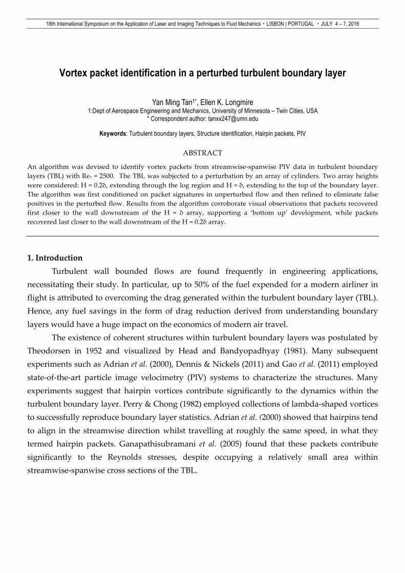
Vortex packet identification in a perturbed turbulent boundary layer

Yan Ming Tan1*, Ellen K. Longmire 1:Dept of Aerospace Engineering and Mechanics, University of Minnesota – Twin Cities, USA

* Correspondent author: [email protected]

Keywords: Turbulent boundary layers, Structure identification, Hairpin packets, PIV

ABSTRACT

An algorithm was devised to identify vortex packets from streamwise-spanwise PIV data in turbulent boundary layers (TBL) with Reτ = 2500. The TBL was subjected to a perturbation by an array of cylinders. Two array heights were considered: H = 0.2δ, extending through the log region and H = δ, extending to the top of the boundary layer. The algorithm was first conditioned on packet signatures in unperturbed flow and then refined to eliminate false positives in the perturbed flow. Results from the algorithm corroborate visual observations that packets recovered first closer to the wall downstream of the H = δ array, supporting a ‘bottom up’ development, while packets recovered last closer to the wall downstream of the H = 0.2δ array.

1. Introduction Turbulent wall bounded flows are found frequently in engineering applications, necessitating their study. In particular, up to 50% of the fuel expended for a modern airliner in flight is attributed to overcoming the drag generated within the turbulent boundary layer (TBL). Hence, any fuel savings in the form of drag reduction derived from understanding boundary layers would have a huge impact on the economics of modern air travel. The existence of coherent structures within turbulent boundary layers was postulated by Theodorsen in 1952 and visualized by Head and Bandyopadhyay (1981). Many subsequent experiments such as Adrian et al. (2000), Dennis & Nickels (2011) and Gao et al. (2011) employed state-of-the-art particle image velocimetry (PIV) systems to characterize the structures. Many experiments suggest that hairpin vortices contribute significantly to the dynamics within the turbulent boundary layer. Perry & Chong (1982) employed collections of lambda-shaped vortices to successfully reproduce boundary layer statistics. Adrian et al. (2000) showed that hairpins tend to align in the streamwise direction whilst travelling at roughly the same speed, in what they termed hairpin packets. Ganapathisubramani et al. (2005) found that these packets contribute significantly to the Reynolds stresses, despite occupying a relatively small area within streamwise-spanwise cross sections of the TBL.


Numerous attempts have been made to manipulate boundary layer behavior by perturbing the flow structure. These attempts can be categorized broadly into two categories: 1) manipulating near-wall structures via surface roughness/non-uniformity; and 2) altering the larger energy-containing motions within and outside of the logarithmic region. The present study falls into the latter group and follows a number of earlier studies. For example, Corke et al (1970) conducted experiments using large eddy breakup (LEBU) devices consisting of ribbon-like devices with large wall normal extent (H/δ = 0.8) and saw reductions of up to 30 – 40% in skin friction drag. Tomkins (2001) looked at the effects of an array of wall-mounted hemispheres (H/δ = 0.09) on the packet organization in the outer layer, and saw a reduction in the streamwise length scales of the packets. Furthermore, coherent structures were altered in regions beyond the height of the perturbation. Other relevant studies include Jacobi & Mckeon (2011) (spanwise bar) and Guala et al. (2012) (hemispheres). The present study follows on the work of Ryan et al. (2011) and Ortiz Duenas et al. (2011) who perturbed the flow with a spanwise array of cylinders with H = 0.2δ. Their PIV results showed that the spacing of the array had a significant effect on the downstream organization of the incoming packet structures. In further work by Zheng and Longmire (2014), the incoming packet organization perturbed by an array with spacing of 0.2δ first disappeared, but then reappeared relatively rapidly downstream. They hypothesized that the reappearance could be explained by the unperturbed packet organization above the array propagating downwards toward the wall. In order to investigate this hypothesis, we conducted PIV experiments downstream of two arrays with 0.2δ spacing and heights H = 0.2δ and H = δ (Tan & Longmire 2015). We applied a feature extraction algorithm to compare the number of low momentum regions (LMRs) downstream of the arrays versus the number in unperturbed flow. The results suggested that, downstream of the array with H = δ, the number of LMRs recovered earliest near the wall. In contrast, the number of LMRs was suppressed closer to the wall behind the array with H = 0.2δ. Other work using feature extraction algorithms to extract packet-like structures or low momentum regions within a TBL includes Ganapathisubramani et al. (2003) and Lin et al. (2008). The former work employed a region-growing algorithm on stereo PIV data in streamwise spanwise planes to extract packet signatures. Regions with large Reynolds stress bounded by strips of positive and negative wall-normal vorticity were used as seed points. Then, neighboring points within a specified range of streamwise velocity were connected such that the final identified region had a relatively uniform (and low) streamwise momentum. Finally, neighboring regions separated by streamwise distance less than their average widths were


merged. Lin et al (2008), on the other hand, employed an algorithm which bears some resemblance to the algorithm presented in this paper to extract features associated with streamwise streaks of low and high momentum in the buffer region. Thresholds dependent on the standard deviation of the streamwise velocity were employed to define coherent regions that were subsequently refined by erosion and dilation of the binarized images. Below, we present an improved feature detection algorithm compared with the one used in Tan and Longmire (2015). The algorithm employs aspects of multiple features to detect and extract individual vortex packets in both unperturbed and perturbed velocity fields derived from planar PIV measurements. 2. Experiment set up Streamwise-spanwise planes of PIV data were acquired in a water channel facility. A trip-wire is located at the entrance to the channel test section, and the boundary layer develops along the bottom wall. At a distance 6m downstream of the trip, the boundary layer height was δ = 125 mm, and Reτ = 2500. In the case of perturbed flow, a single spanwise array of cylinders was mounted at this streamwise location. In the rest of the paper, the streamwise, spanwise and wall normal directions are denoted by x, y, and z, where x = 0 corresponds to the location of the cylinder array. U and V are used to denote streamwise and spanwise velocity respectively. Two array heights were considered: H = 0.2δ (or H+ = 500) and H = δ, and the cylinder diameter was held constant at D = 6.35 mm. Cylinders were spaced at 0.2δ in both arrays. PIV data was acquired at three measurement heights: z+ = 125, z+ = 300 and z+ = 500, extending over the log region. Data was acquired at six streamwise stations downstream of the array location. The furthest downstream location was centered on x/δ = 7. Two TSI 4MP PowerView Cameras were used simultaneously to obtain wide fields of view corresponding with 1.1δ x 2.2δ in the streamwise and spanwise directions respectively. The resolution of the PIV data was ~2.2 mm or ~40 wall units. Using a 50% overlap, the vector spacing of the data was ~1.1mm or ~20 wall units. The sampling rate was roughly 0.5 Hz, and 1000 independent samples were acquired at every measurement location. The uncertainty in each component of the instantaneous PIV vectors was 0.01U∞. 3. Vortex packet identification algorithm (VPIA)

As the VPIA was to be used for comparison purposes, i.e. perturbed vs. unperturbed flow, we sought to identify only ‘individual’ packets not complicated by spanwise merging structures. In addition, packets intersecting the spanwise edges of the PIV fields were not


considered. Furthermore, the algorithm was devised to be restrictive, i.e. our strategy was to minimize false positives, rather than to identify every individual packet within the data. Under this restriction, we aimed to capture as many individual packets as possible. Based on previous literature and the authors’ experience in scanning through many instantaneous streamwise-spanwise fields, we define packets as coherent slow moving regions bounded by counter rotating swirls (signed by wall-normal vorticity direction). In this context, swirl or swirling strength is defined as the imaginary part of the eigenvalues of the two-component velocity gradient tensor, where in this case, swirling structures could be cross sections of hairpin legs. The essence of the algorithm is to employ image processing techniques in MATLAB to automatically extract and catalogue packets with criteria guided by the authors’ experience viewing many instances of packet signatures. The algorithm was conditioned based on packets observed in the unperturbed flow, then applied to perturbed data.

The algorithm description is as follows:

Step 1: A threshold was applied to the PIV velocity data to identify regions of U < 0.95Um

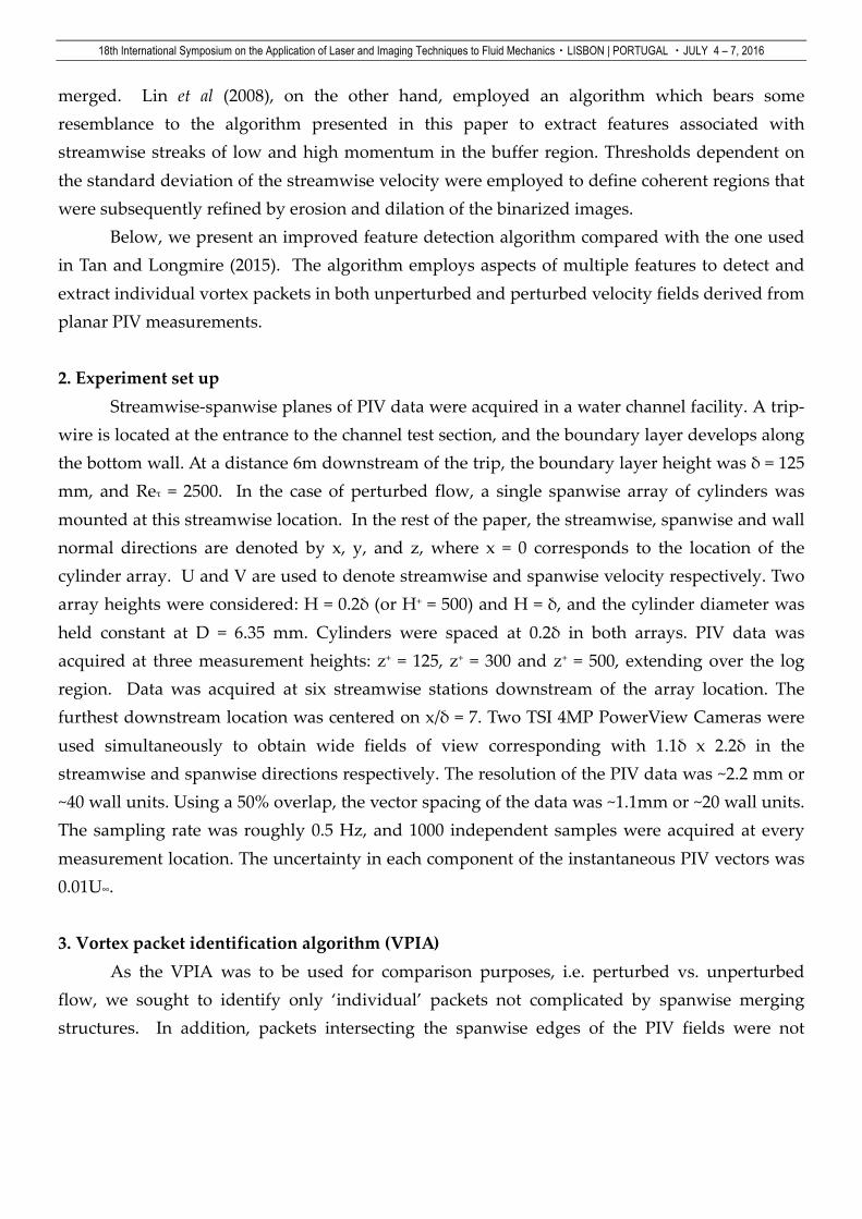
where Um is the mean velocity at the measurement height. Step 2: The thresholded velocity field was binarized, and MATLAB image processing functions were used to detect connected regions. Step 3: The length, width and orientation of the detected regions were computed. The length and width were determined based on the streamwise and spanwise extrema of the detected region respectively. The orientation was determined by fitting an ellipse to the outline of the structure, and taking the angle between the major axis and the streamwise direction. Minimum thresholds were set for the length (0.5δ) and width (0.05δ) in order to extract structures with significant streamwise and spanwise extent. Additionally, structures with large inclinations to the streamwise direction (>25°) were removed. The output of Steps 1 through 3 applied to a sample unperturbed field is shown in Figure 1b. Step 4: Erosion and dilation were performed on the structures identified through step 3 to separate loosely connected regions. The output of this step was fed through to step 3 again to eliminate separated structures that now failed the length, width or orientation criteria specified previously. The resulting output for the sample field is shown in Figure 1c. The erosion and


Figure 1. VPIA process on a sample field and its respective intermediate outputs. a) Sample input to VPIA,

intermediate outputs after b) steps 1-3, c) step 4 & 5, d) after steps 6-7

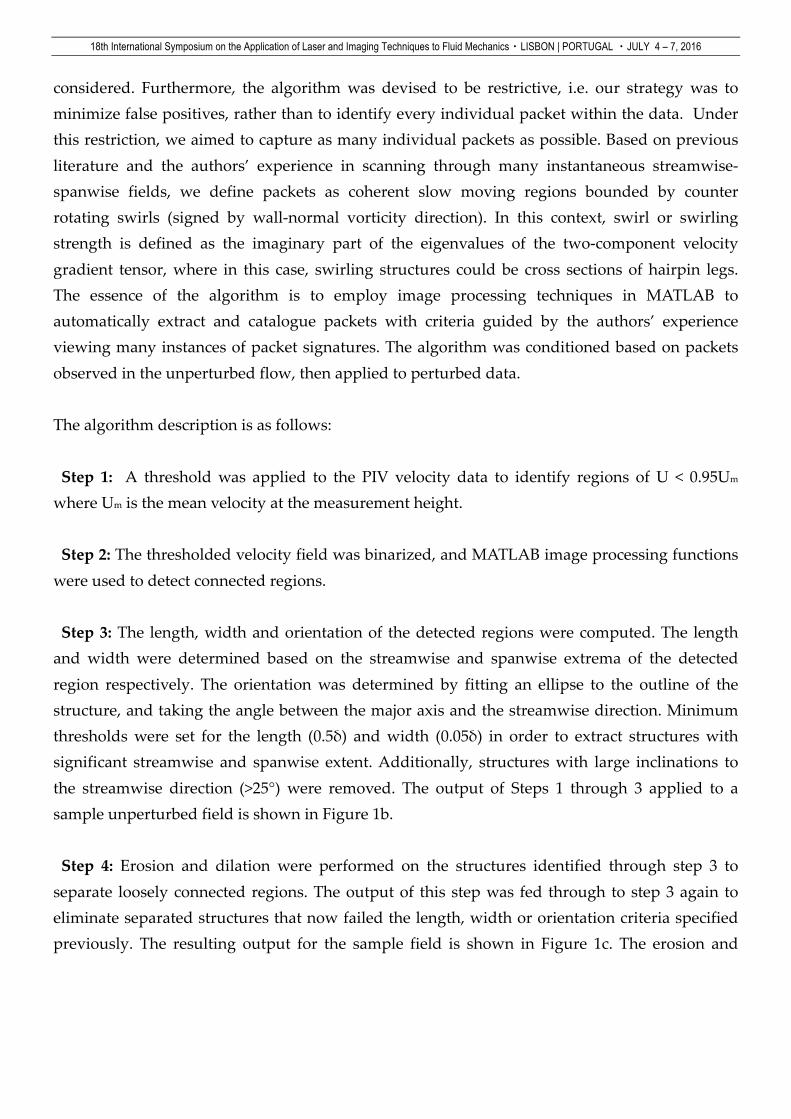
dilation separated several weakly-connected regions, and some separated structures were eliminated after failing the minimum length criterion. Step 5: Streamwise scans of the remaining structures were performed in order to construct a skeleton. First, the width of the structure at every streamwise location was computed and averaged, to acquire an estimate of the mean width. Then, the skeleton was constructed by connecting regions for which the local width was greater than 60% of the mean width. Structures with large gaps in the skeleton (> 10 grid points) were removed as they did not look like packets. An example of a detected skeleton in unperturbed flow is shown in Figure 2a. Figure 2b shows an identified structure from perturbed flow that was removed due to the large gap in its skeleton. Step 6: The swirling strength, λci, was computed where the velocity gradients were obtained via central difference and normalized by the freestream velocity and δ. A threshold of |λci| > 2.5 was applied, and the resulting swirl fields were binarized. This threshold was selected to suppress noise whilst retaining swirl structures that appear to indicate cross sections of hairpin legs. Using similar connection and extraction methods as in steps 1-2, all swirls were detected

PIV field 1. U < 0.95Um

2. Binarize 3. Length + Width + Orientation

4. Erosion + dilation 5. construct skeleton

6. |λci| > 2.5 7. Establish λci

connectivity

a) b))

c) d)


Figure 2. Sample skeletons acquired from the streamwise scan of the structure width

and labeled. The minimum length and width of the detected structures based on the extrema was set at 3 grid points.

Step 7: Swirling regions overlapping the detected low momentum regions (LMRs) were identified. The number of swirls per length (Ns/L) and the ratio of positive to negative swirls (Ns+/s-) associated with each LMR were computed. Figure 1d shows all swirling structures that have been associated with the detected LMRs. The steps described above were applied to sets of 100 PIV fields for unperturbed flow at all three measurement heights. Then, the structures identified were compared manually against the original PIV plots that overlaid swirling structures and streamwise velocity contours (e.g. Figure 1a). Structures identified by the algorithm were separated into the following categories: packets, non-packets, merging/merged packets, and edge structures. The comparison revealed a number of false positives at each height. To decrease the number of false positives, threshold criteria based on Ns+/s- and Ns/L were added. The former was used to eliminate structures that intersected the spanwise edges of the field, while the latter helped eliminate merged/merging structures. Additionally, both criteria were effective at eliminating some structures that lacked associated swirls. The threshold values can be found in Table 1. After applying these additional criteria at z+ = 125 and z+ = 300 in the unperturbed flow, no non-packets were present in the VPIA output from the data sets examined. On the other hand, 3% of the detected structures at z+ = 500 were classified as non-packets. At all measurement heights, a small number of structures detected were classified as merged/merging packets. These structures were difficult to remove as their statistics could closely resemble those of individual packet signatures. More restrictive thresholds on Ns/L could exclude these structures but only at a cost of losing a greater number of individual packets. Nevertheless, this was not seen as a critical problem in assessing relative differences between perturbed and unperturbed fields. The algorithm, including the additional thresholds on Ns+/s- and Ns/L, was next applied to the perturbed boundary layer data at downstream locations greater than x/δ = 2.4. To evaluate

a) b)


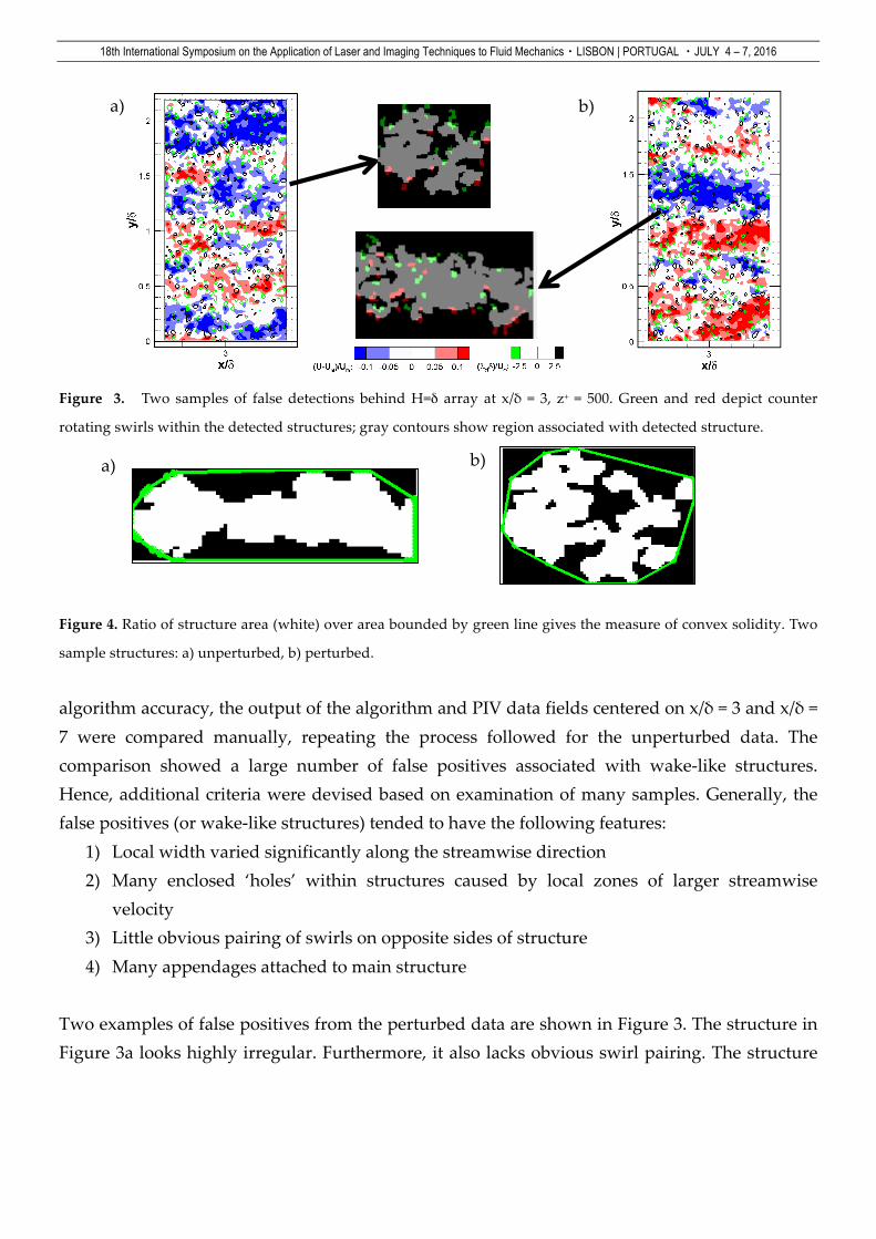
Figure 3. Two samples of false detections behind H=δ array at x/δ = 3, z+ = 500. Green and red depict counter

rotating swirls within the detected structures; gray contours show region associated with detected structure.

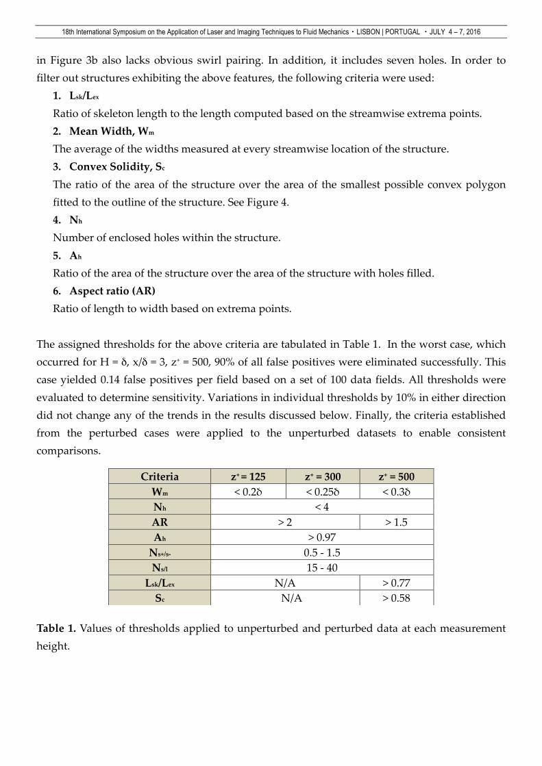
Figure 4. Ratio of structure area (white) over area bounded by green line gives the measure of convex solidity. Two

sample structures: a) unperturbed, b) perturbed.

algorithm accuracy, the output of the algorithm and PIV data fields centered on x/δ = 3 and x/δ = 7 were compared manually, repeating the process followed for the unperturbed data. The comparison showed a large number of false positives associated with wake-like structures. Hence, additional criteria were devised based on examination of many samples. Generally, the false positives (or wake-like structures) tended to have the following features:

1) Local width varied significantly along the streamwise direction 2) Many enclosed ‘holes’ within structures caused by local zones of larger streamwise

velocity 3) Little obvious pairing of swirls on opposite sides of structure 4) Many appendages attached to main structure

Two examples of false positives from the perturbed data are shown in Figure 3. The structure in Figure 3a looks highly irregular. Furthermore, it also lacks obvious swirl pairing. The structure

a) b)

a) b)


in Figure 3b also lacks obvious swirl pairing. In addition, it includes seven holes. In order to filter out structures exhibiting the above features, the following criteria were used:

1. Lsk/Lex Ratio of skeleton length to the length computed based on the streamwise extrema points. 2. Mean Width, Wm The average of the widths measured at every streamwise location of the structure. 3. Convex Solidity, Sc The ratio of the area of the structure over the area of the smallest possible convex polygon fitted to the outline of the structure. See Figure 4. 4. Nh Number of enclosed holes within the structure. 5. Ah Ratio of the area of the structure over the area of the structure with holes filled. 6. Aspect ratio (AR) Ratio of length to width based on extrema points.

The assigned thresholds for the above criteria are tabulated in Table 1. In the worst case, which occurred for H = δ, x/δ = 3, z+ = 500, 90% of all false positives were eliminated successfully. This case yielded 0.14 false positives per field based on a set of 100 data fields. All thresholds were evaluated to determine sensitivity. Variations in individual thresholds by 10% in either direction did not change any of the trends in the results discussed below. Finally, the criteria established from the perturbed cases were applied to the unperturbed datasets to enable consistent comparisons. Table 1. Values of thresholds applied to unperturbed and perturbed data at each measurement height.

Criteria z+ = 125 z+ = 300 z+ = 500 Wm < 0.2δ < 0.25δ < 0.3δ Nh < 4 AR > 2 > 1.5 Ah > 0.97

Ns+/s- 0.5 - 1.5 Ns/l 15 - 40

Lsk/Lex N/A > 0.77 Sc N/A > 0.58


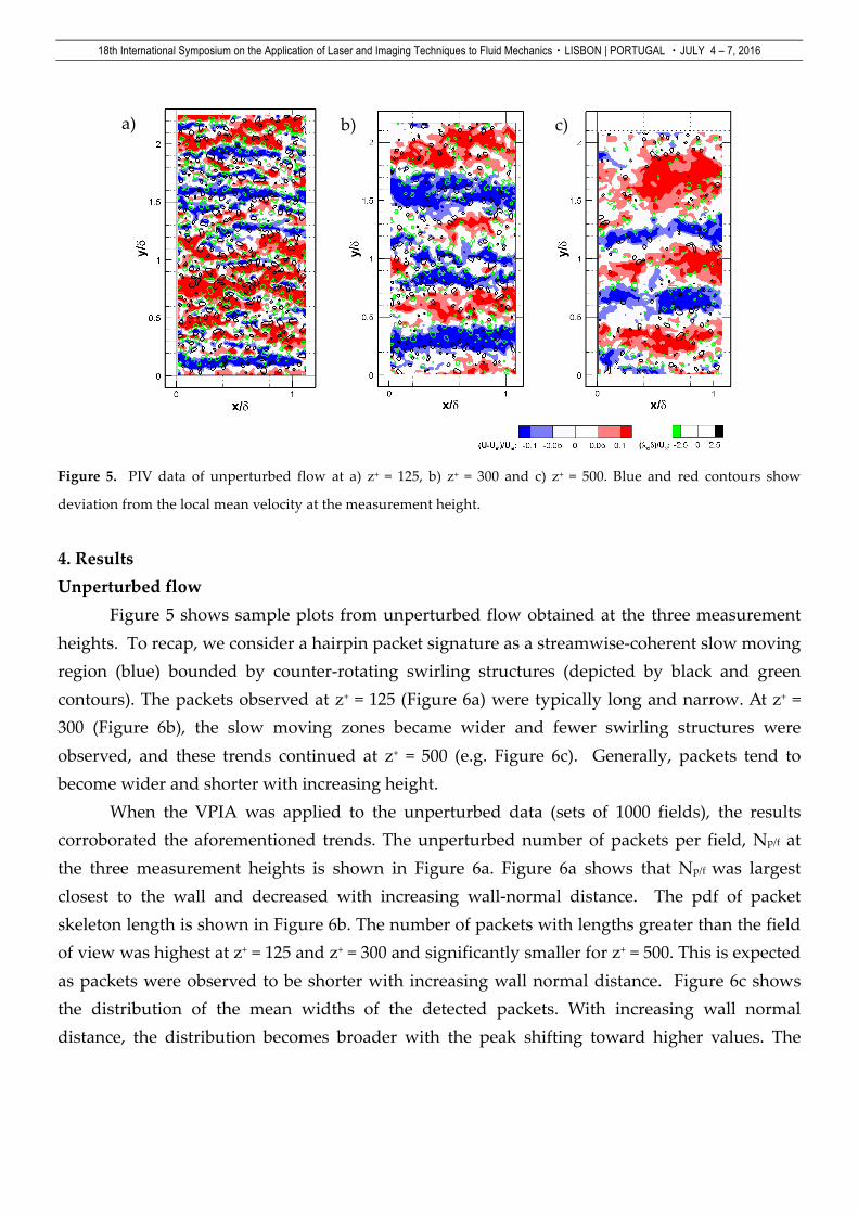
Figure 5. PIV data of unperturbed flow at a) z+ = 125, b) z+ = 300 and c) z+ = 500. Blue and red contours show

deviation from the local mean velocity at the measurement height.

4. Results Unperturbed flow

Figure 5 shows sample plots from unperturbed flow obtained at the three measurement heights. To recap, we consider a hairpin packet signature as a streamwise-coherent slow moving region (blue) bounded by counter-rotating swirling structures (depicted by black and green contours). The packets observed at z+ = 125 (Figure 6a) were typically long and narrow. At z+ = 300 (Figure 6b), the slow moving zones became wider and fewer swirling structures were observed, and these trends continued at z+ = 500 (e.g. Figure 6c). Generally, packets tend to become wider and shorter with increasing height.

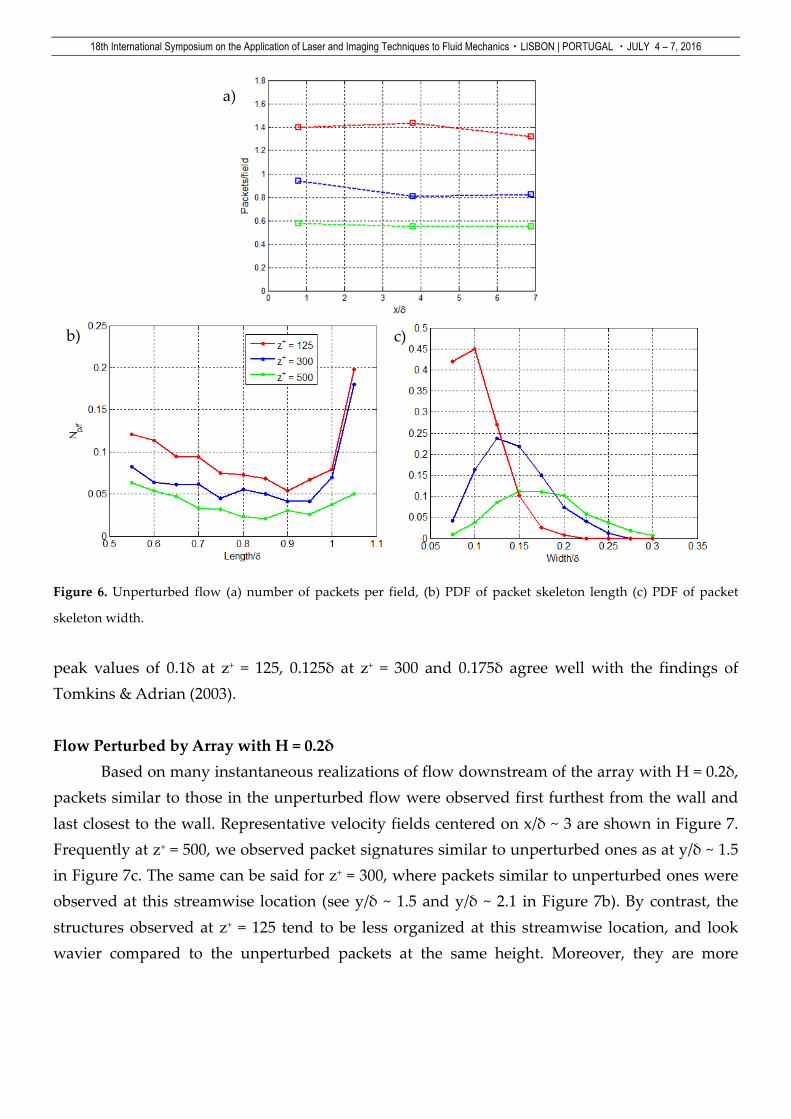
When the VPIA was applied to the unperturbed data (sets of 1000 fields), the results corroborated the aforementioned trends. The unperturbed number of packets per field, Np/f at the three measurement heights is shown in Figure 6a. Figure 6a shows that Np/f was largest closest to the wall and decreased with increasing wall-normal distance. The pdf of packet skeleton length is shown in Figure 6b. The number of packets with lengths greater than the field of view was highest at z+ = 125 and z+ = 300 and significantly smaller for z+ = 500. This is expected as packets were observed to be shorter with increasing wall normal distance. Figure 6c shows the distribution of the mean widths of the detected packets. With increasing wall normal distance, the distribution becomes broader with the peak shifting toward higher values. The

a) b) c)


Figure 6. Unperturbed flow (a) number of packets per field, (b) PDF of packet skeleton length (c) PDF of packet

skeleton width. peak values of 0.1δ at z+ = 125, 0.125δ at z+ = 300 and 0.175δ agree well with the findings of Tomkins & Adrian (2003).

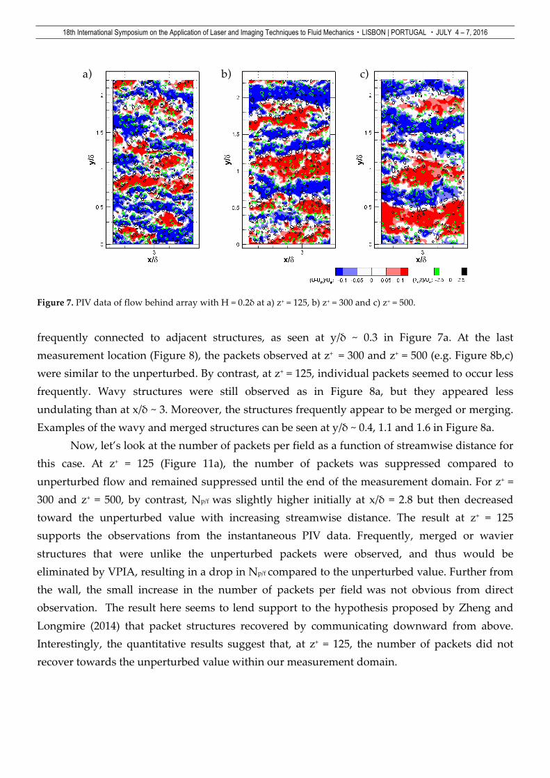
Flow Perturbed by Array with H = 0.2δ Based on many instantaneous realizations of flow downstream of the array with H = 0.2δ, packets similar to those in the unperturbed flow were observed first furthest from the wall and last closest to the wall. Representative velocity fields centered on x/δ ~ 3 are shown in Figure 7. Frequently at z+ = 500, we observed packet signatures similar to unperturbed ones as at y/δ ~ 1.5 in Figure 7c. The same can be said for z+ = 300, where packets similar to unperturbed ones were observed at this streamwise location (see y/δ ~ 1.5 and y/δ ~ 2.1 in Figure 7b). By contrast, the structures observed at z+ = 125 tend to be less organized at this streamwise location, and look wavier compared to the unperturbed packets at the same height. Moreover, they are more

a)a)

b) c)


Figure 7. PIV data of flow behind array with H = 0.2δ at a) z+ = 125, b) z+ = 300 and c) z+ = 500.

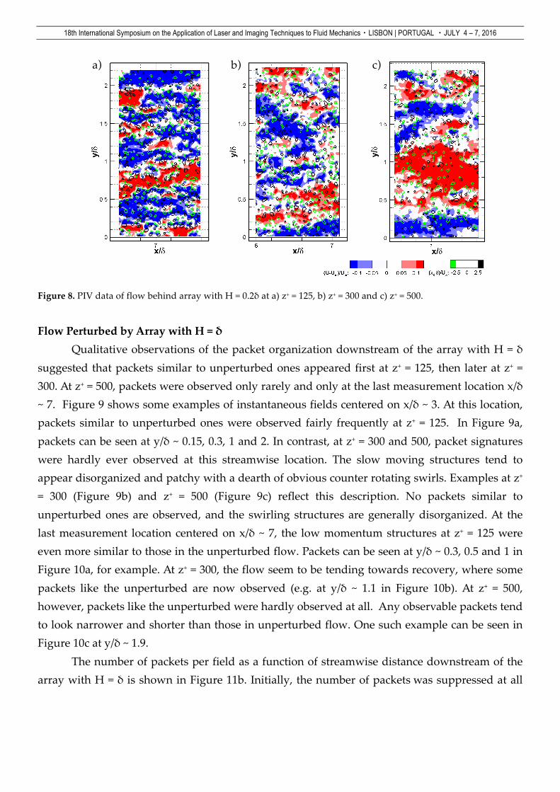
frequently connected to adjacent structures, as seen at y/δ ~ 0.3 in Figure 7a. At the last measurement location (Figure 8), the packets observed at z+ = 300 and z+ = 500 (e.g. Figure 8b,c) were similar to the unperturbed. By contrast, at z+ = 125, individual packets seemed to occur less frequently. Wavy structures were still observed as in Figure 8a, but they appeared less undulating than at x/δ ~ 3. Moreover, the structures frequently appear to be merged or merging. Examples of the wavy and merged structures can be seen at y/δ ~ 0.4, 1.1 and 1.6 in Figure 8a.

Now, let’s look at the number of packets per field as a function of streamwise distance for this case. At z+ = 125 (Figure 11a), the number of packets was suppressed compared to unperturbed flow and remained suppressed until the end of the measurement domain. For z+ = 300 and z+ = 500, by contrast, Np/f was slightly higher initially at x/δ = 2.8 but then decreased toward the unperturbed value with increasing streamwise distance. The result at z+ = 125 supports the observations from the instantaneous PIV data. Frequently, merged or wavier structures that were unlike the unperturbed packets were observed, and thus would be eliminated by VPIA, resulting in a drop in Np/f compared to the unperturbed value. Further from the wall, the small increase in the number of packets per field was not obvious from direct observation. The result here seems to lend support to the hypothesis proposed by Zheng and Longmire (2014) that packet structures recovered by communicating downward from above. Interestingly, the quantitative results suggest that, at z+ = 125, the number of packets did not recover towards the unperturbed value within our measurement domain.

a) b) c)


Figure 8. PIV data of flow behind array with H = 0.2δ at a) z+ = 125, b) z+ = 300 and c) z+ = 500.

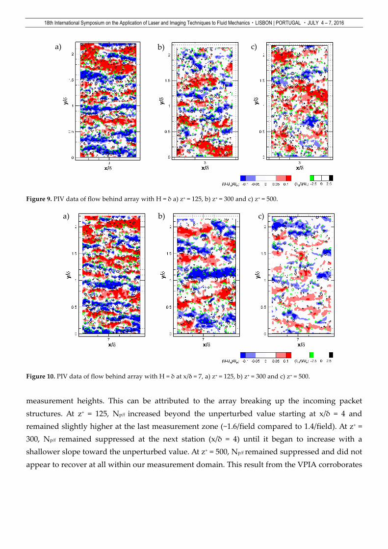
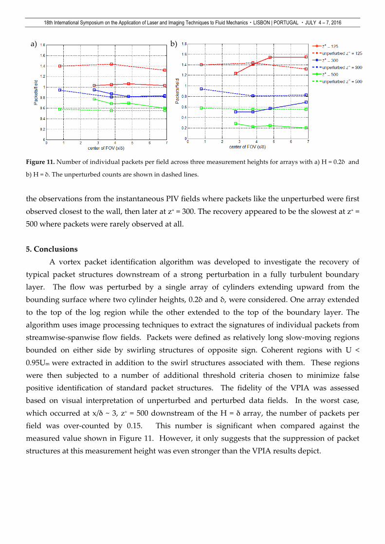
Flow Perturbed by Array with H = δ Qualitative observations of the packet organization downstream of the array with H = δ suggested that packets similar to unperturbed ones appeared first at z+ = 125, then later at z+ = 300. At z+ = 500, packets were observed only rarely and only at the last measurement location x/δ ~ 7. Figure 9 shows some examples of instantaneous fields centered on x/δ ~ 3. At this location, packets similar to unperturbed ones were observed fairly frequently at z+ = 125. In Figure 9a, packets can be seen at y/δ ~ 0.15, 0.3, 1 and 2. In contrast, at z+ = 300 and 500, packet signatures were hardly ever observed at this streamwise location. The slow moving structures tend to appear disorganized and patchy with a dearth of obvious counter rotating swirls. Examples at z+ = 300 (Figure 9b) and z+ = 500 (Figure 9c) reflect this description. No packets similar to unperturbed ones are observed, and the swirling structures are generally disorganized. At the last measurement location centered on x/δ ~ 7, the low momentum structures at z+ = 125 were even more similar to those in the unperturbed flow. Packets can be seen at y/δ ~ 0.3, 0.5 and 1 in Figure 10a, for example. At z+ = 300, the flow seem to be tending towards recovery, where some packets like the unperturbed are now observed (e.g. at y/δ ~ 1.1 in Figure 10b). At z+ = 500, however, packets like the unperturbed were hardly observed at all. Any observable packets tend to look narrower and shorter than those in unperturbed flow. One such example can be seen in Figure 10c at y/δ ~ 1.9. The number of packets per field as a function of streamwise distance downstream of the array with H = δ is shown in Figure 11b. Initially, the number of packets was suppressed at all

c) b) a)


Figure 9. PIV data of flow behind array with H = δ a) z+ = 125, b) z+ = 300 and c) z+ = 500.

Figure 10. PIV data of flow behind array with H = δ at x/δ = 7, a) z+ = 125, b) z+ = 300 and c) z+ = 500.

measurement heights. This can be attributed to the array breaking up the incoming packet structures. At z+ = 125, Np/f increased beyond the unperturbed value starting at x/δ = 4 and remained slightly higher at the last measurement zone (~1.6/field compared to 1.4/field). At z+ = 300, Np/f remained suppressed at the next station (x/δ = 4) until it began to increase with a shallower slope toward the unperturbed value. At z+ = 500, Np/f remained suppressed and did not appear to recover at all within our measurement domain. This result from the VPIA corroborates

a) b) c)

a) b) c)


Figure 11. Number of individual packets per field across three measurement heights for arrays with a) H = 0.2δ and

b) H = δ. The unperturbed counts are shown in dashed lines.

the observations from the instantaneous PIV fields where packets like the unperturbed were first observed closest to the wall, then later at z+ = 300. The recovery appeared to be the slowest at z+ = 500 where packets were rarely observed at all. 5. Conclusions A vortex packet identification algorithm was developed to investigate the recovery of typical packet structures downstream of a strong perturbation in a fully turbulent boundary layer. The flow was perturbed by a single array of cylinders extending upward from the bounding surface where two cylinder heights, 0.2δ and δ, were considered. One array extended to the top of the log region while the other extended to the top of the boundary layer. The algorithm uses image processing techniques to extract the signatures of individual packets from streamwise-spanwise flow fields. Packets were defined as relatively long slow-moving regions bounded on either side by swirling structures of opposite sign. Coherent regions with U < 0.95Um were extracted in addition to the swirl structures associated with them. These regions were then subjected to a number of additional threshold criteria chosen to minimize false positive identification of standard packet structures. The fidelity of the VPIA was assessed based on visual interpretation of unperturbed and perturbed data fields. In the worst case, which occurred at x/δ ~ 3, z+ = 500 downstream of the H = δ array, the number of packets per field was over-counted by 0.15. This number is significant when compared against the measured value shown in Figure 11. However, it only suggests that the suppression of packet structures at this measurement height was even stronger than the VPIA results depict.

a) b)


The VPIA results from the unperturbed data revealed the greatest number of individual packets closest to the wall (z+ = 125), with decreasing numbers as z+ increased. Moreover, the results indicated that packets at z+ = 125 were narrower and longer, and became wider and shorter with increasing wall normal distance, consistent with Tomkins & Adrian (2003). Downstream of the H = 0.2δ array, visual observations indicated that packets recovered sooner at z+ = 300 than at z+ = 125, consistent with the hypothesis proposed by Zheng and Longmire (2014) that the incoming organization above the array persisted and communicated downwards toward the wall. In contrast, downstream of the array with H = δ, packets were observed first closer to the wall and later further from the wall. The VPIA results on number of packets per field were consistent with these visual observations and with the idea of bottom-up growth suggested by Adrian et al. (2000). Both the VPIA and visual results suggested that the overall structure at the top of the log layer (z+ = 500, z = 0.2δ) remained far from equilibrium at 7δ downstream of the perturbation which was the end of the measurement domain. References Adrian, R.J., Meinhart, C.D. and Tomkins, C.D. 2000. “Vortex Organization in the outer region of the turbulent boundary layer.” J. Fluid Mech. 422: 1-54 Corke, T.C., Guezennec, Y. and Nagib, H.M. 1981. “Modification in drag of turbulent boundary layers resulting from manipulation of large- scale structures” NASA CR- 3444 Dennis., D.J.C., Nickels, T.B. 2011. “Experimental measurement of large-scale three-dimensional structures in a turbulent boundary layer. Part 1. Vortex packets.” J. Fluid Mech. 673:180 – 219. Ganapathisubramani, B., Longmire, E.K., Marusic I. 2003. “Characteristics of vortex packets in turbulent boundary layers.” J. Fluid Mech. 478: 35-46 Gao, Q., Ortiz-Dueñas, C., and Longmire E. K. 2011. “Analysis of vortex populations in turbulent wall-bounded flows.” J. Fluid Mech. 678:87–123. Guala, M., Tomkins, C. D., Christensen, K. T., and Adrian, R.J. 2012. “Vortex organization in a turbulent boundary layer overlying sparse roughness elements.” Journal of Hydraulic Research 50:465–481. Head., M.R., Bandyopadhyay, P. 1981. “New aspects of turbulent boundary-layer structure.” J. Fluid Mech. 107: 297 – 338. Jacobi, I., and McKeon, B. J. 2011. “New perspectives on the impulsive roughness-perturbation of a turbulent boundary layer.” J. Fluid Mech. 677:179–203. Lin. J., Laval, J.P., Foucaut, J.M., Stanislas, M., 2008. “Quantitative characterization of coherent structures in the buffer layer of near-wall turbulence. Part 1: streaks.” Exp. Fluids. 45:999-1013. Ortiz-Dueñas, C., Ryan, M.D., and Longmire, E. K. 2011. “Modification of Turbulent Boundary Layer Structure Using Immersed Wall- Mounted Cylinders.” Proc. Turbulent Shear Flow Phenomena VIII, Ottawa. Perry., A.E., Chong, M.S. 1982. “On the mechanism of wall turbulence.” J. Fluid Mech. 119: 173-217.


Ryan, M.D., Ortiz-Dueñas, C., and Longmire, E. K. 2011. “Effects of Simple Wall-Mounted Cylinder Arrangements on a Turbulent Boundary Layer.” AIAA Journal. 49(10):2210–2220. Tan, Y.M and Longmire, E.K. 2015 “On the reorganization of perturbed hairpin packets in a turbulent boundary layer.” Proceedings 11th International symposium on particle image velocimetry, Santa Barbara, CA. Theodorsen, T. 1952. Mechanism of turbulence. Proc. Second Midwestern Conf. of Fluid Mechanics. Tomkins CD and Adrian RJ. 2003 “Spanwise structure and scale growth in turbulent boundary layers.” J.Fluid Mech. 490: 37-74 Tomkins, C.D., 2001. “The structure of turbulence over smooth and rough walls”. Ph.D. Thesis, University of Illinois at Urbana Champaign. Zheng, S., and Longmire. E. K. 2014. “Perturbing vortex packets in a turbulent boundary layer.” J. Fluid Mech. 748:368–398.

Documents

Vortex packet identification in a perturbed turbulent ...ltces.dem.ist.utl.pt/lxlaser/lxlaser2016/finalworks2016/papers/03... · 18th International Symposium on the Application of