Department of Economics

Master’s Thesis

Supervisor: Eva Mörk

VOTING SYSTEM

VOTER TURNOUT

POLICY OUTCOME

Linuz Aggeborn

2

Abstract

In the last decades a number of countries in the developed world have experienced a drop in

voter turnout. The public sector is in the end run by politicians who are elected by the people

and for that reason it is interesting to study how a variation in turnout will affect public policy

outcome. The purpose of this master’s thesis is to investigate the potential causal link that

runs between voting system, turnout and policy by empirically testing the Meltzer &

Richard’s theory from 1981. I use Swedish and Finnish municipal panel data and apply IV-

regression. The constitutional change in 1970 when Sweden changed from having separate

election days for the central and the local governments into having one joint election day, is

used as instrument for turnout. I find that an increased turnout rate also leads to higher local

tax rate indicating that turnout actually has an impact on policy outcome.

Keywords: Turnout, Policy outcome, IV-regression, Difference-in Difference, Sweden,

Finland

Acknowledgement: This thesis highly benefitted from comments by my supervisor Professor

Eva Mörk. I also wish to thank Professor Matz Dahlberg for the dataset regarding Swedish

state grants and Olle Storm at SCB for explaining old Swedish municipal statistics and

providing me with parts of the data being used. Furthermore I would like to thank Björn

Tyrefors-Hinnerich for the data regarding Swedish municipal mergers and residents in the

Swedish municipalities for the earlier years. Furthermore I would like to express gratitude

towards Statistikcentralen in Finland for explaining Finnish municipal financial statistics and

especially Mikko Mehtonen. I am also grateful to Tore Ivarsson for explaining the municipal

merger reform in Sweden. Lastly I would like to thank seminar participants at Uppsala

University.

3

Table of Contents

1. Introduction ................................................................................................................................4

1.1. Related work ...................................................................................................................6

2. Theory ...................................................................................................................................... 10

2.1. Hypothesis ......................................................................................................................... 17

3. Data .......................................................................................................................................... 18

4. Econometric model ................................................................................................................... 22

5. Institutional background ............................................................................................................ 25

6. Results ...................................................................................................................................... 31

7. Robustness checks..................................................................................................................... 38

8. Discussion................................................................................................................................. 40

9. Conclusion ................................................................................................................................ 42

10. References .............................................................................................................................. 44

Appendix ...................................................................................................................................... 48

4

1. Introduction

Over the last decades, a number of democratic countries in the developed world have

observed a decline in voter turnout. The decline varies between countries, but also between

different types of elections, where especially the decrease in voter turnout in local elections

has been more severe. 1 Political Scientist Arend Lijphart has argued that a drop in voter

turnout should be seen as a crisis for democracy as the legitimacy for the democratic process

is damaged. 2 According to standard Political Scientist’s point of view, democracy and a high

participation rate is seen as something positive per se and the issue of voter turnout decline

has therefore been an area of extensive research.3

Parallel to the trend of decline in voter turnout, the developed nations have

experienced a growth of the public sector on both the national and the local level. 4 The

political arena in a democracy is in the end run by politicians, who are elected by the people.

Within the field of Political Economy, voting and democracy have often not an intrinsic value

but are merely considered as means of aggregating preferences of individuals. Naturally,

different political decisions result in different political policies. Uncontroversial to say,

different policy outcome will affect economic outcomes in various ways too. The political

arena is thus an important and significant economic entity affecting the economy both directly

and indirectly. The act of voting, as a mean of aggregating preferences, is therefore interesting

to study within Political Economics since it constitutes the core of the public sector.

Understanding how variations in voter turnout affect policy outcome should be of major

interest given that the size of the public sector is significant.

The above issues are much related to the topic of how the voting system is

designed. 5

The decline in voter turnout may be the overall trend in developed countries, but

there are still significant differences between them. According to Lijphart, who believe that

we have an obligation of increasing voter turnout rate, mandatory voting, a proportional

voting system and a low cost associated with voting, i.e. a single election day on a week-end

and uncomplicated registration procedures should increase voter turnout.6 Standard rational

1 Lijphart, Arend: 1996, p. 5 ff 2 Ibid, p. 1 f 3See for example Franklin, Mark: 1999, Electoral Engineering and Cross-National Turnout Differences: What

Role for Compulsory Voting? Ruy, Teixeiran:1987, Why Americans don’t vote, turnout decline in the united

states 1960 - 1985 4 Rosen, Harvey & Gayer, Ted: 2008, p. 7 5 For example of studies that have investigated what will determine voter turnout rate, see for example Jackman,

Robert, 1987 Political institutions and voter turnout in industrialized democracies, Sigelman et al: 1985 Voting

an Non-voting, a multielection perspective and Blais, André: 2005, What affects voter turnout? 6 Lijphart, Arend:1996, p. 1

5

choice theory also predicts that if the cost of voting is decreased, voter turnout rate will

increase.7 It is however relatively hard to define and measure cost. In order to investigate if

cost will influence the choice of participation, one must find a very concrete example where

cost is either high or low. There is one particular detail in the voting system which in a very

direct way relates to the discussion of cost and may constitute an adequate example: The

clustering of different types of elections. A number of countries in the developed world have

today separate election days for parliamentary elections and local/regional elections. Some

countries have however chosen a system where elections to some, or all, levels of government

are grouped into a single election day.8 If election days are separated, the cost of voting has

increased and we should expect a lower voter turnout rate according to the predictions of

rational choice theory. The relationship between voting system and turnout and between

turnout and policy outcome is an issue that has not been analyzed in itself but merely in

separate studies in either Political Science or Economics.

The purpose of this master’s thesis is to investigate the potential causal link that

runs between voting system, turnout and policy outcome. More precisely, the purpose is to

estimate the effect of turnout on policy outcome using the voting system as an instrument.

Swedish and Finnish municipal panel data is used for the time period 1964 – 1999

where the change in the Swedish voting system in 1970 from a system with separate election

days into a system with one common election day constitutes the instrument. Just as it is

possible to imagine that turnout may affect policy outcome it is also plausible that the effect

runs in the other direction, i.e. policy outcome might influence the participation choice of

individuals. In order to deal with this simultaneous causality threat, an IV-regression approach

will be applied. Secondly, I will also investigate the reduced formed, that is if there is a

difference in policy outcome after the change in the voting system by performing a classical

difference-in-difference analysis where the Swedish municipalities constitute the treatment

group and the Finnish municipalities the control group.

In this thesis I will merge Meltzer & Richard’s (1981) A rational theory of the size

of government with classical rational choice theory regarding democratic participation.

According to Meltzer & Richard (1981), policy outcome will change when the voting rule

changes. Is there any empirical evidence of such a claim? The inclusion of more people into

the electorate generates a higher degree of redistribution and consequently a higher tax rate if

the median voter has a lower income than the mean income holder in the society according to

7 Mueller, Dennis: 2003 p. 303 ff

8 SOU 2001:65 , p.20

6

Meltzer & Richard (1981). Along the lines of classical rational choice theory, the cost of

voting will affect the choice of participating. The analysis of the first-stage in the IV-

regression (if the introduction of a common election day increases turnout) is interesting in

itself since this answer the question if a change in the voting system affects turnout and

consequently contribute to the discussion whether cost will influence participation. If we

assume that those with a higher education and a higher income has a elevated taste for the act

of voting9 the change from separate election day into a voting system with one common

election day should generate a relatively higher turnout in low income groups resulting in a

policy outcome with more redistribution and higher taxes. Does a variation in turnout affect

policy outcome?

The thesis consists of six main parts. First of all, I will discuss earlier work that has

addressed similar research questions in order to place my thesis in a context. Then follows the

theoretical section where Meltzer & Richard’s (1981) A rational theory of the size of

government is presented and discussed. The data section describes the data set and gives

background information regarding Finnish and Swedish municipalities. The econometric

section sets up the econometric model where I also discuss the indentifying assumption

behind my chosen empirical strategy. In the institutional background section, Swedish and

Finnish municipalities are further presented. The empirical setting in this thesis rest on the

assumption of a large similarity between Sweden and Finland and therefore evidence of this is

presented here. Subsequently follow results, robustness checks, discussion and conclusion.

I find that voter turnout will affect policy outcome as a higher turnout rate

increases the municipal tax rate. I also find by analyzing the reduced form that changing the

voting system has an effect on policy outcome where a common election day yields an

increased tax rate. These effects are both statistically and economically significant if the

whole time period is considered.

1.1. Related work

There is a void in the research field of Political Economics when it comes to the potential

connection between voting system, voter turnout and policy outcome. Very few studies have

addressed how a variation in turnout will affect conducted policy. By linking this issue to the

discussion of common versus separate election days it is possible to connect the interesting

9 This is also in line with the arguments presented in Lijphart (1996)

7

discussion regarding a potential class bias in policy as a result of a change in the electorate to

the discussion if the cost associated with voting will affect the turnout rate.

Mueller & Stratmann (2002) investigate if turnout in itself will affect policy and

economic outcome. They use panel data ranging from 1960 to 1990 for a large number of

countries and investigate how income equality, size of the public sector and economic growth

are affected by a variation in turnout. Their main result is that a lower turnout has a significant

effect of creating a higher gini-coefficient, i.e. a less equal income distribution. A higher

turnout is associated with a larger public sector and as a result a lower economic growth.

They do not find evidence that higher turnout in itself lower economic growth.10

Mueller &

Stratmann (2002) used cross country data, which I believe is not optimal for the issue at hand.

Countries tend to be rather different from each other and act in separate macroeconomic

contexts. Even when including a large number of suitable covariates it is relatively logical to

argue that there are still important unobserved characteristics remaining between the countries

included in the analysis. My chosen dataset where I use municipal panel data from two

countries very similar in institutional setting is more appropriate when investigating the causal

link between turnout and policy outcome in my opinion.

Caplan (2007) declares that the median voter is in fact irrational and that the

electorate has a systematic bias in its beliefs in comparison to a simulated “enlighten public”

as well in comparison to the expressed opinions by educated economists. 11

The extension of

the argument is that a high turnout will only enforce this systematic bias. Since high-educated

people are more prone to vote, a lower turnout would then result in a smaller bias in the

electorate and change the political and economic outcome to the better. This is a more elite-

oriented view towards democratic participation which takes a normative stance on the issue.

Caplan (2007) acknowledge that a variation in turnout will affect economic policy, but instead

of seeing this as a problem in line with a participation based argument for democracy12

, he

believes that this should be seen as something positive. In this thesis I am not going to discuss

which policy outcome is more favorable than the other. First of all, this is beyond the purpose

of this thesis; furthermore it is relatively hard to argue that some preferences are scientifically

better than others without giving separate weights to different utility functions for different

groups in a society.

10 Mueller, Dennis & Stratmann, Thomas: 2002, p. 2151 11 Caplan, Bryan: 2007: p. 198 12 Participation based argument for democracy rest on the belief that the democratic participation has a value in

itself. Elections are conducted in order to aggregate the opinions and preferences of the people. A high turnout is

thus a necessity and the core in a democratic society.

8

As already noted, there are not many papers that focus on how variations in turnout

affect policy outcome. There are on the other hand several papers which focus on how

different political systems affect policy outcome. The purpose of this essay is to use the

voting system as an instrument in order to investigate if turnout affect policy outcome. I will

however also present the reduced form of this econometric analysis, i.e. if the voting system

induces a different policy outcome13

. Let us briefly look at some papers that have focused on

this relationship.

Persson (2002) found, by using a cross-country panel data set, that the

constitutional setting in a country will affect economic outcome. A majority voting system

seems to generate a more slimmed well-fare state where public spending is targeted towards

swing-voters by the politicians in order to win elections. In addition, a majority voting system

is also linked with a lower degree of corruption. In a country with a proportional voting

system, each vote counts and therefore spending is to a larger extent focused on a broader

group of people.14

Boix (1999) argues that the setting of the voting system is a product of utility

maximizing political parties. By performing an historical analysis of the choice between a

majority system and a proportional voting system (PR) he found that countries tend to choose

the system that favors parties that have previously been in power. Changing from one system

to the other in quite uncommon, but might occur if a previously dominant party feels

threatened by the demographic development and/or a change in the preferences of (certain

parts of) the electorate. 15

This paper is interesting since it argues that the voting system

should be viewed as an endogenous variable. Boix (1999) does not address the issue of

common versus separate election days; however the same line of argument may be applied on

this matter as well. Political parties which believe that they will be favored by a common

election day will support such a system and vice versa.

When suffrage was extended to women during the 19th and 20th centuries for a

number of countries in the world, the electorate grew to a large extent. Lott & Kenny (1999)

investigate if the growth of government in the late the 19th and 20th century can be explained

by the inclusion of women into the electorate. They concluded that the extended suffrage

resulted in increased government spending and more liberal policies overall in the votes of the

House of Representatives and the Senate in the U.S. Congress. This conclusion is noteworthy

13 The whole effect is assumed to go through turnout in this thesis. 14

Persson, Torsten: 2002, p. 902 f 15 Boix, Charles: 1999, p. 23 ff

9

since it indicates that a change in the voting rule in a country actually results in different

policy outcomes. 16

If we define a voting rule as a rule that decide or influence which groups

in a society that will vote; a constitutional setting with a common election day and a system

with separate election days may then been seen as two different voting rules. Based on the

results in Lott & Kenny (1999) there is reason to believe that policy outcome will change

when shifting from a voting system with separate election days into a voting system with one

common election day.

Based on earlier works, we suspect that there will be some policy difference

between a system with a common and a system with separate election days. Fumagalli &

Narciso (2008) have drawn some preliminary conclusions in a discussion paper where they

use the same dataset as in Persson (2002). They argue that voter turnout is the intermediate

link between the constitutional setting and economic outcome. First of all, constitutional

setting will affect voter turnout. Second of all, voter turnout will have a positive and

statistically significant effect on government spending and the size of the public sector. 17

This study is the first and only attempt to my knowledge, to connect the discussions regarding

constitutional setting, voter turnout and policy outcome to each other. The paper also

highlights the importance of connecting these three phenomena together which is why I will

present the first and second stage in the IV-regression as well as the reduced form. However,

Fumagalli & Narciso (2008) is mainly empirical and does not provide any theoretical

explanation why the framing of the voting system will affect turnout and why this will affect

policy outcome. Furthermore, a cross-country data approach as in Persson (2002) and

Fumagalli & Narciso (2008) is associated with several obstacles which I have already

discussed.

The choice between one common versus separate election days and how this would

affect voter turnout has been addressed in several Swedish official reports. The reason for this

is mainly that Sweden has a common election day, although several political parties in the

Swedish parliament favor a system with separate election days.18

All of these reports argue

much in line with standard rational choice theory, saying that if the cost associated with

voting is increased, voter turnout will decrease. If elections are held on separate days the cost

16 Lott, John & Kenny, Lawrence: 1999, p. 1163 17 Fumagalli, Eileen & Narciso, Gaia: 2008, p. 8 ff 18 First of all Grundlagsutredningen, addressed the issue and came to the conclusion that separate election days

would probably decrease turnout. Two other official reports, Demokratiutredningen and Värdet av

valdeltagande, also consist of sections discussing the potential change in voter turnout when changing to a

system with separate election days. The same yield for the official report Skilda valdagar och vårval. SOU

2008:125, p. 173 ff, SOU:2000:1 p. 189 f, SOU 2007: 84, SOU 2001:65

10

has increased with the result of lower turnout in both national and local elections. The

problem with all of these official reports is that they do not address the issue of causality in a

suitable way. The empirical method used is based on a cross-section method where different

countries are compared to each other. 19

A more suitable design would be a difference-in-

difference approach where the outcome in the treatment group, before and after treatment, are

compared to the before and after outcome in the control group. The control group should in

this case be very similar to the treatment group; a relationship which I believe is fulfilled

between Finland and Sweden. 20

2. Theory

According to standard rational choice theory, the decision of voting is based on rationality.

There is some personal utility associated with having your preferred candidate or party

winning the election, but there is also some cost, C, associated with voting. This cost may be

defined in various ways, depending of the framing of the voting system. In some countries,

one must register before voting with the potential risk of being selected to jury duty (USA). In

a totalitarian country, the cost of voting, or more precisely voting on the wrong candidate,

might result in execution, i.e. an extremely high cost associated with voting. Two more

concrete examples of cost associated with voting in a democratic country are the cost of

transportation to the polling station and the alternative cost of time spent on finding

information about the parties in an election. A rational individual vote if the benefit, B, of

having the preferred candidate/party winning the election times the actual probability of being

the decisive voter in the election is greater than the cost associated with voting21

according to

the following formula:

0PB C (1)

The probability that you will be the decisive voter in an election is in most cases very small

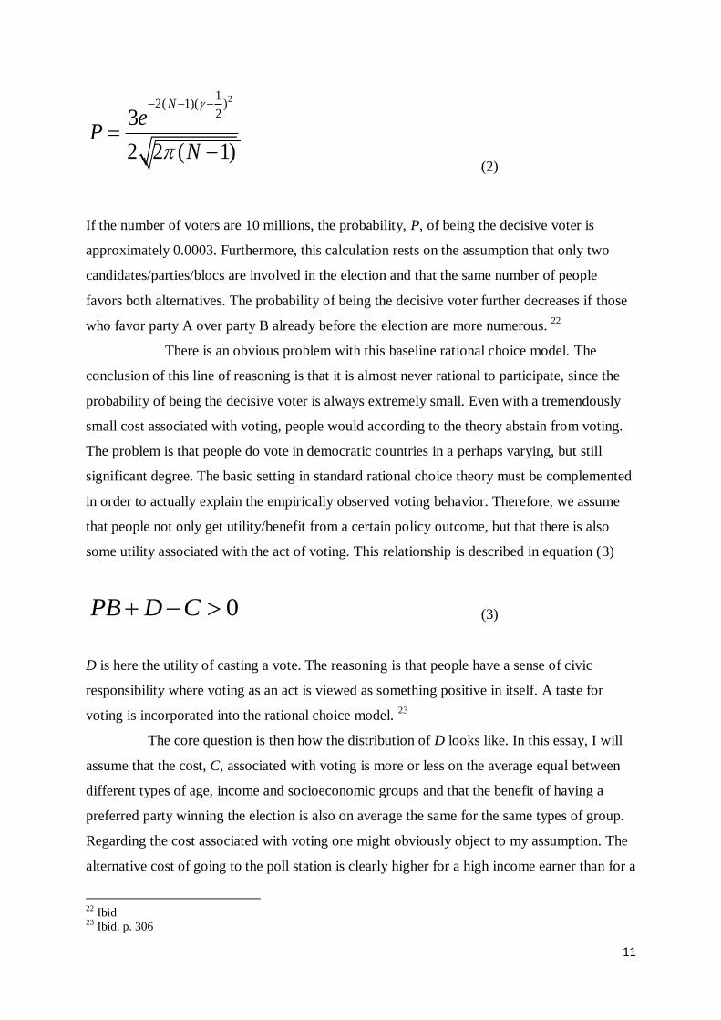
and the probability further decreases when the size of the electorate becomes larger and can

be calculated according to the formula below:

19 Mueller, Dennis: 2003 p. 304 ff, SOU 2001:65, passim 20

See my Institutional background section. 21 Mueller, Dennis: 2003, p. 303 ff

11

(2)

If the number of voters are 10 millions, the probability, P, of being the decisive voter is

approximately 0.0003. Furthermore, this calculation rests on the assumption that only two

candidates/parties/blocs are involved in the election and that the same number of people

favors both alternatives. The probability of being the decisive voter further decreases if those

who favor party A over party B already before the election are more numerous. 22

There is an obvious problem with this baseline rational choice model. The

conclusion of this line of reasoning is that it is almost never rational to participate, since the

probability of being the decisive voter is always extremely small. Even with a tremendously

small cost associated with voting, people would according to the theory abstain from voting.

The problem is that people do vote in democratic countries in a perhaps varying, but still

significant degree. The basic setting in standard rational choice theory must be complemented

in order to actually explain the empirically observed voting behavior. Therefore, we assume

that people not only get utility/benefit from a certain policy outcome, but that there is also

some utility associated with the act of voting. This relationship is described in equation (3)

0PB D C (3)

D is here the utility of casting a vote. The reasoning is that people have a sense of civic

responsibility where voting as an act is viewed as something positive in itself. A taste for

voting is incorporated into the rational choice model. 23

The core question is then how the distribution of D looks like. In this essay, I will

assume that the cost, C, associated with voting is more or less on the average equal between

different types of age, income and socioeconomic groups and that the benefit of having a

preferred party winning the election is also on average the same for the same types of group.

Regarding the cost associated with voting one might obviously object to my assumption. The

alternative cost of going to the poll station is clearly higher for a high income earner than for a

22

Ibid 23 Ibid. p. 306

212( 1)( )

23

2 2 ( 1)

N

eP

N

12

low income earner. However, in both Sweden and Finland elections are always held on

Sundays24

thus reducing the difference in alternative cost between different income groups

since people usually do not work on Sundays.

It is however not realistic at all to assume that the level of D does not vary between

different socioeconomic groups in the society. It is reasonable to presuppose that D is

correlated with years of schooling which is also correlated with income. 25

A higher education

gives on average a higher degree of social capital which gives rise to a greater interest in

society and a higher probability of voting. 26 Consider the central component in this essay,

namely a common versus separate election days; when having separate election days for

national and local assemblies, people have to go to the polling station twice as often and the

cost of voting therefore increases. A common election day and separate election days

constitute two different voting rules. If the cost associated with voting is increased, voter

turnout will decrease, but relatively more in those groups with a lower degree of taste from

voting, since the level of D to some extent can compensate for a higher C. A common election

day would relatively speaking induce more people to vote and increase the share of people

belonging to lower socioeconomic groups in the electorate.

The central question is then how a variation in turnout is connected to policy

outcome. The politicians are assumed in this thesis to be decisive when it comes to decisions

regarding taxation and redistribution of income. If we start with the classical median voter

theorem first laid out by Hotelling & Downs it has been proven that it is the median voter in

the electorate that is the decisive voter. Regardless if politicians are office motivated or policy

motivated it is rational for them to propose policy in line with the preferences of the median

voter in order to maximize their level of utility. According to the Hotelling & Downs model,

voter turnout is not a factor and the median voter is just equal to the median citizens regarding

political preferences. 27

Meltzer & Richard (1981) further developed the ideas laid out by Hotelling & Downs

by incorporating a discussion regarding the composition of the electorate. 28

A voting rule is

defined as a rule that will determine who will be the decisive voter in a population. A

dictatorship has the voting rule that only one person decides and this person is obviously then

24 Dahlberg, Matz & Mörk, Eva: 2011, p. 8 25 Borjas, George: 2008, p. 274 f 26 Lijphart, Arend: 1996, p. 3 27 Meltzer, Allan H & Richards, Scott: 1981, p. 916 28 Ibid, p. 914. Note that the whole theoretical section in this essay is based on the Meltzer & Richard (1981)

theory and that the equations also come from the same paper. I have not chosen to present all of the

mathematical derivations behind this theory. Please see the original paper for more details.

13

the decisive voter. In a democracy, a spectrum of potential voting rules is present. 29

In

accordance with the Hotelling & Downs theory, the decisive voter is equal to the median

voter in the electorate but the electorate in itself might be different in political systems with

different voting rules. As a consequence, the decisive voter will still be the median voter, but

the median voter is not the same when the voting rule is different since the electorate has

changed. What are the potential policy outcome consequences of such a shift in the

electorate?

The decisive voter, i.e. the median voter, is assumed to have a preference for the level

of distribution of income in the society and logically a preference for the tax level in order to

obtain the desired distribution level. People are assumed to be rational and realize that a

higher degree of distribution of income presumes a higher level of income tax. The decisive

individual will determine his preference for redistribution and tax rate by maximizing his

personal level of utility. The personal utility will be determined by two separate variables:

Consumption and leisure time. First of all, the decisive voter/the median voter, will choose

more redistribution if the mean income in the society is higher than his own in order to

increase his level of consumption. The extension of this line of reasoning is that he has

preference for a higher level of income tax. The decisive voter is however rational and

realizes that his choice of tax level will not only affect his own personal economic situation

but also everyone else’s. People will react to economic incentives and a higher level of

income tax will influence the labor leisure choice of the other consumers in the economy. The

basic idea behind the theory of labor leisure choice is based on standard consumer choice

theory, theorizing that a person has a limited amount of time and that he gets utility from both

consumption and leisure time. In order to consume, a person is in need of an income and in

order to get income, he must work according to 30

(4)

where T is the initial time endowment. C is the amount of consumption, w the wage

and leisure time. According to this very simple model, a higher degree of redistribution is

then translated into a higher degree of C that is not related to a lower degree of (leisure)

29

Ibid, p. 920 30 Ibid. p. 917

C w T

14

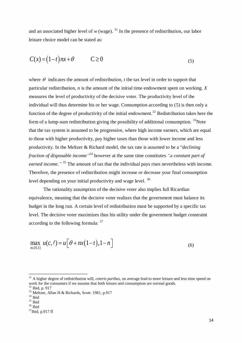
and an associated higher level of w (wage). 31

In the presence of redistribution, our labor

leisure choice model can be stated as:

(5)

where indicates the amount of redistribution, t the tax level in order to support that

particular redistribution, n is the amount of the initial time endowment spent on working. X

measures the level of productivity of the decisive voter. The productivity level of the

individual will thus determine his or her wage. Consumption according to (5) is then only a

function of the degree of productivity of the initial endowment.32

Redistribution takes here the

form of a lump-sum redistribution giving the possibility of additional consumption. 33

Note

that the tax system is assumed to be progressive, where high income earners, which are equal

to those with higher productivity, pay higher taxes than those with lower income and less

productivity. In the Meltzer & Richard model, the tax rate is assumed to be a “declining

fraction of disposable income”34

however at the same time constitutes “a constant part of

earned income.” 35

The amount of tax that the individual pays rises nevertheless with income.

Therefore, the presence of redistribution might increase or decrease your final consumption

level depending on your initial productivity and wage level. 36

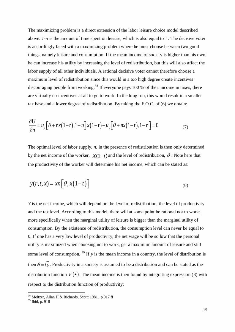
The rationality assumption of the decisive voter also implies full Ricardian

equivalence, meaning that the decisive voter realizes that the government must balance its

budget in the long run. A certain level of redistribution must be supported by a specific tax

level. The decisive voter maximizes thus his utility under the government budget constraint

according to the following formula: 37

(6)

31 A higher degree of redistribution will, ceteris paribus, on average lead to more leisure and less time spend on

work for the consumers if we assume that both leisure and consumption are normal goods. 32 Ibid, p. 917 33 Meltzer, Allan H & Richards, Scott: 1981, p.917 34 Ibid 35 Ibid 36

Ibid 37Ibid, p.917 ff

( ) 1 C 0C x t nx

[0,1]

max ( , ) 1 ,1n

u c u nx t n

15

The maximizing problem is a direct extension of the labor leisure choice model described

above. 1-n is the amount of time spent on leisure, which is also equal to . The decisive voter

is accordingly faced with a maximizing problem where he must choose between two good

things, namely leisure and consumption. If the mean income of society is higher than his own,

he can increase his utility by increasing the level of redistribution, but this will also affect the

labor supply of all other individuals. A rational decisive voter cannot therefore choose a

maximum level of redistribution since this would in a too high degree create incentives

discouraging people from working.38

If everyone pays 100 % of their income in taxes, there

are virtually no incentives at all to go to work. In the long run, this would result in a smaller

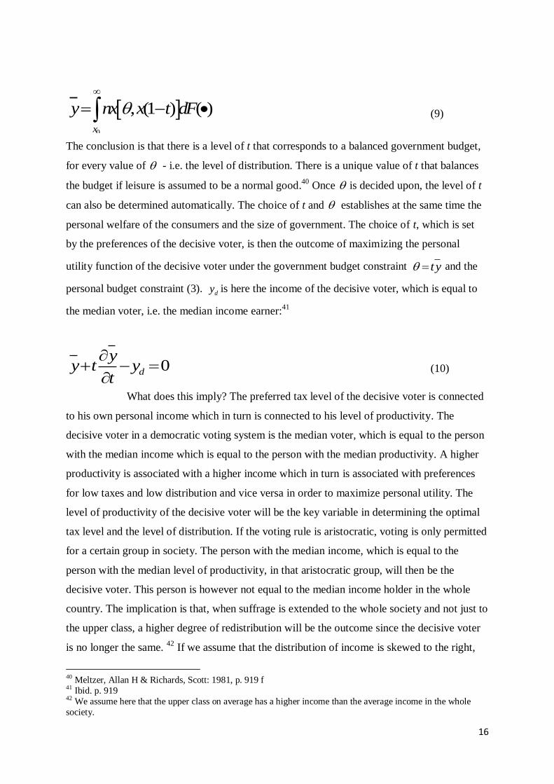
tax base and a lower degree of redistribution. By taking the F.O.C. of (6) we obtain:

(7)

The optimal level of labor supply, n, in the presence of redistribution is then only determined

by the net income of the worker, and the level of redistribution, . Note here that

the productivity of the worker will determine his net income, which can be stated as:

(8)

Y is the net income, which will depend on the level of redistribution, the level of productivity

and the tax level. According to this model, there will at some point be rational not to work;

more specifically when the marginal utility of leisure is bigger than the marginal utility of

consumption. By the existence of redistribution, the consumption level can never be equal to

0. If one has a very low level of productivity, the net wage will be so low that the personal

utility is maximized when choosing not to work, get a maximum amount of leisure and still

some level of consumption. 39

If is the mean income in a country, the level of distribution is

then . Productivity in a society is assumed to be a distribution and can be stated as the

distribution function . The mean income is then found by integrating expression (8) with

respect to the distribution function of productivity:

38

Meltzer, Allan H & Richards, Scott: 1981, p.917 ff 39 Ibid, p. 918

1 ,1 1 1 ,1 0c

Uu nx t n x t u nx t n

n

(1 )X t

( , , ) , 1y r t x xn x t

y

t y

F

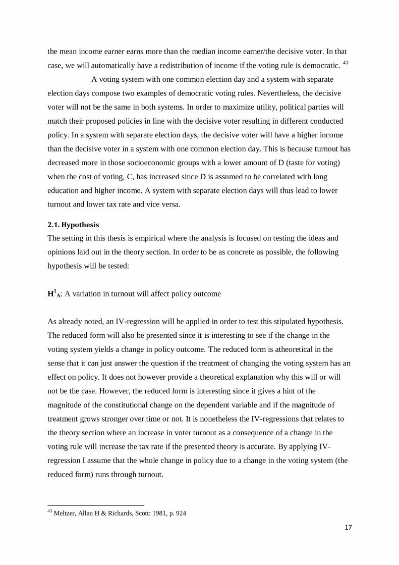
16

(9)

The conclusion is that there is a level of t that corresponds to a balanced government budget,

for every value of - i.e. the level of distribution. There is a unique value of t that balances

the budget if leisure is assumed to be a normal good.40

Once is decided upon, the level of t

can also be determined automatically. The choice of t and establishes at the same time the

personal welfare of the consumers and the size of government. The choice of t, which is set

by the preferences of the decisive voter, is then the outcome of maximizing the personal

utility function of the decisive voter under the government budget constraint and the

personal budget constraint (3). is here the income of the decisive voter, which is equal to

the median voter, i.e. the median income earner:41

(10)

What does this imply? The preferred tax level of the decisive voter is connected

to his own personal income which in turn is connected to his level of productivity. The

decisive voter in a democratic voting system is the median voter, which is equal to the person

with the median income which is equal to the person with the median productivity. A higher

productivity is associated with a higher income which in turn is associated with preferences

for low taxes and low distribution and vice versa in order to maximize personal utility. The

level of productivity of the decisive voter will be the key variable in determining the optimal

tax level and the level of distribution. If the voting rule is aristocratic, voting is only permitted

for a certain group in society. The person with the median income, which is equal to the

person with the median level of productivity, in that aristocratic group, will then be the

decisive voter. This person is however not equal to the median income holder in the whole

country. The implication is that, when suffrage is extended to the whole society and not just to

the upper class, a higher degree of redistribution will be the outcome since the decisive voter

is no longer the same. 42

If we assume that the distribution of income is skewed to the right,

40 Meltzer, Allan H & Richards, Scott: 1981, p. 919 f 41 Ibid. p. 919 42

We assume here that the upper class on average has a higher income than the average income in the whole

society.

0

, (1 ) ( )x

y nx x t dF

t y

dy

0d

yy t y

t

17

the mean income earner earns more than the median income earner/the decisive voter. In that

case, we will automatically have a redistribution of income if the voting rule is democratic. 43

A voting system with one common election day and a system with separate

election days compose two examples of democratic voting rules. Nevertheless, the decisive

voter will not be the same in both systems. In order to maximize utility, political parties will

match their proposed policies in line with the decisive voter resulting in different conducted

policy. In a system with separate election days, the decisive voter will have a higher income

than the decisive voter in a system with one common election day. This is because turnout has

decreased more in those socioeconomic groups with a lower amount of D (taste for voting)

when the cost of voting, C, has increased since D is assumed to be correlated with long

education and higher income. A system with separate election days will thus lead to lower

turnout and lower tax rate and vice versa.

2.1. Hypothesis

The setting in this thesis is empirical where the analysis is focused on testing the ideas and

opinions laid out in the theory section. In order to be as concrete as possible, the following

hypothesis will be tested:

H1

A: A variation in turnout will affect policy outcome

As already noted, an IV-regression will be applied in order to test this stipulated hypothesis.

The reduced form will also be presented since it is interesting to see if the change in the

voting system yields a change in policy outcome. The reduced form is atheoretical in the

sense that it can just answer the question if the treatment of changing the voting system has an

effect on policy. It does not however provide a theoretical explanation why this will or will

not be the case. However, the reduced form is interesting since it gives a hint of the

magnitude of the constitutional change on the dependent variable and if the magnitude of

treatment grows stronger over time or not. It is nonetheless the IV-regressions that relates to

the theory section where an increase in voter turnout as a consequence of a change in the

voting rule will increase the tax rate if the presented theory is accurate. By applying IV-

regression I assume that the whole change in policy due to a change in the voting system (the

reduced form) runs through turnout.

43 Meltzer, Allan H & Richards, Scott: 1981, p. 924

18

The question is if this is realistic. There are those who argue that separate election

days generate a higher degree of information in the electorate which in turn will influence

policy outcome.44

It is possible to relate the political opinions regarding separate election days to the

ideas of Jürgen Habemas. According to Habemas, democracy should be based on a good

conversation where the ideal is the academic seminar where different ideas and opinions are

discussed. By having a good political discussion, the political ideas are improved as people

get a better understanding of them and their implications. A well-functioning communication

between individuals will result in a higher degree of rationality. 45

When having a common

election day, the political discussion concerning national, regional and local politics will be

clustered into a single time period before the election day. The result, according to the

argument of Habemas, is a decreased level of rationality, which in turn might affect the policy

outcome. This reasoning is in line with discussion based argument of democracy.46

This is a suggestion how one could understand the political arguments from

politicians who are pro separate election days and are not the explicit work and ideas laid out

by Habemas. These opinions are however not based on any economic theory and therefore I

will continue to argue that the whole potential change in policy will be due to a variation in

turnout when using the voting system as an instrument in accordance with the ideas laid out in

the theory section. In order to investigate if the level of information affects policy outcome

one must have access to a data set measuring the degree of information in the electorate. In

future studies it might be interesting to test whether a change from a system with separate

election days into a system with a common election day, actually generates a lower degree of

information and vice versa but this is not the scope of this thesis.

3. Data

In order to empirically test my stipulated hypotheses, the ideal dataset would contain

observations from one single country where different regions are very similar in institutional

setting and the composition of the electorate, with the only difference that some parts of the

country have a common election day and other parts have separate election days. Potentially,

a reform changing the voting system that has not been implemented at the same time all over

44 In Sweden five out of eight parties in parliament are pro separate election days. Their main argument is that

the degree of information will be increased by such a reform. SOU 2001:65, p. 64 45 Bolton, Roger: 2005, passim 46 Discussion based argument for democracy rest of the opinion that all decision making will be improved if it is

preceded by a rational discussion. The ideal is the academic seminar where conflicting ideas and empirical facts

are discussed and evaluated. The democratic process is to be considered as a better framing in order to create a

better and more universal discussion.

19

the country can be used. However, such a dataset is not very likely to exist. Therefore I chose

to use municipal panel data from Sweden and Finland in order to test my hypothesis. Sweden

abolished the bicameral parliamentary system in 1970 and as a result introduced one common

election day for national, regional and local election. Before 1970, elections to the county

counsels and municipal councils were conducted in-between parliamentary elections. Finland

on the other hand has had separate election days since the introduction of universal suffrage

until today. 47

The change from a system with separate election days into a system with one

common election day is thus considered as the treatment of interest in this study when

analyzing the reduced form. The counterfactual treatment is continuing having separate

election days. The time period analyzed is 1964-1999.

Both Sweden and Finland have a long tradition of gathering reliable and detailed

statistics which suits the purpose of this thesis very well. The similar institutional setting

between Finland and Sweden forms a very appropriate testing ground for empirically oriented

research in Political Economics. The data used in this paper mainly comes originally from

SCB and Statistikcentralen. Data earlier than 1974 is not available in digital form and has

therefore been manually inputted from Årsbok för Sveriges kommuner, Kommunal

finansstatistik Finland, Årsbok för Finland and Kommunalvalen 1970, 1968, 1966 and 1964

for Sweden and Finland respectively. For details regarding the data, see the reference list.

One core question is which dependent variable I will use in order to test my

hypothesis. Several potential policy outcome variables exist and in upcoming studies it might

be interesting to focus on different aspects regarding policy outcome. I will however choose

to focus on municipal tax rate in this thesis. The theory laid out by Meltzer & Richards (1981)

focuses on income redistribution and in order to redistribute, the government must collect

taxes. The variable municipal tax rate grasps the core components in the Meltzer & Richard

theory in my point of view.

Control variables are evidently needed in the analysis in order to compensate for

potential omitted variable bias. I will add population in each municipal and state grants per

capita as control variables. Tax base between Sweden and Finland will also be added, also

expressed in per capita, for a shorter time period but as two different variables since there is a

slight difference in the definition between the Swedish and the Finnish municipal data

47

Dahlberg, Matz & Mörk, Eva: 2011, p. 7 f , Statistikcentralen, val, kommunalval & riksdagsval, beskrivning

av statistik. SOU 2001:65 p. 12

20

regarding tax base.48

Data regarding tax base in not available in digital form and has therefore

to be manually inputted for all years, which is the reason for only using these variables for a

shorter time period. In an upcoming study it would be interesting to add further control

variables such as age and education structure in each municipal in order to get more precise

estimates.

One prominent challenge in my econometrical analysis is to find a way to deal

with the presence of municipal mergers which took place in Sweden during 1965 to 1973.

Municipalities were merged in order to create a more efficient local level of government. 49

Finnish municipal mergers have also taken place but have been more sporadic and not that

concentrated in time.50

Between 1965 and 1974 Swedish municipalities were reduced from

approximately 1000 to a little less than 300.51

I have chosen those Swedish municipalities that

remained after the municipal mergers was over in 1974 (in total a little less than 300) in my

analysis in order to get a rather constant number of observations each year over time. Since

the mergers took place in the same time period as Sweden introduced a common election day,

i.e. my chosen instrument, I must investigate if a potential merging-effect is present. I will

control for population size in my regression, but also the tax base in each municipal since

these variables did increase substantially when mergers took place. Furthermore I will also

examine if we have heterogeneity in the estimates. I will analyze separately those Swedish

municipalities that were actually merged with other municipalities and those who were not in

my robustness checks section.

The variable turnout only changes value every fourth year in Finland for the

entire time period and every third year in Sweden between 1970-1994 and every fourth year

for the remaining years since elections are not held every year. I choose to view turnout as

constant over one mandate period, i.e. turnout remains the same for sequential years up until

the next election. I believe that this setting is suitable since a turnout rate logically does have

an impact on local political assemblies and policy for the entire period and not just the same

48 The Swedish tax base expresses the total declared income of taxable income whereas the Finnish tax base is

expressed in the sum of tax to the municipalities. For the earlier years, the definition between Finland and

Sweden regarding tax base does not make it possible to convert the data into one single variable. 49 Tyrefors-Hinnerich, Björn: 2009, p. 722 f 50 Mergers of Finnish municipalities have been rather intense after 1999 and are thus something that does not

concern my study. During my time periods mergers does take place in the Finnish dataset. Normally, a smaller

municipality seizes to exist and become part of a larger municipality when the inhabitants share is considered as

to small. By including population as a control variable I can control for a sudden increase of persons in a

municipality. The Finnish municipal mergers are rather different from the Swedish municipal mergers were

municipalities were forced to merge during a rather short time period in the latter case. 51 Tyrefors-Hinnerich, Björn: 2009, p. 722 f

21

year as elections takes place. The variable turnout does not therefore report a missing value

for the years between elections.

The municipalities of Åland have been dropped from the analysis since these

municipalities have different responsibilities and administrative structure than the other

municipalities in Finland.52

The Swedish municipalities of Gotland, Gothenburg and Malmö

have also been dropped because they have the responsibilities of municipal well-fare services

together with the well-fare services that usually sort under the counties in Sweden.53

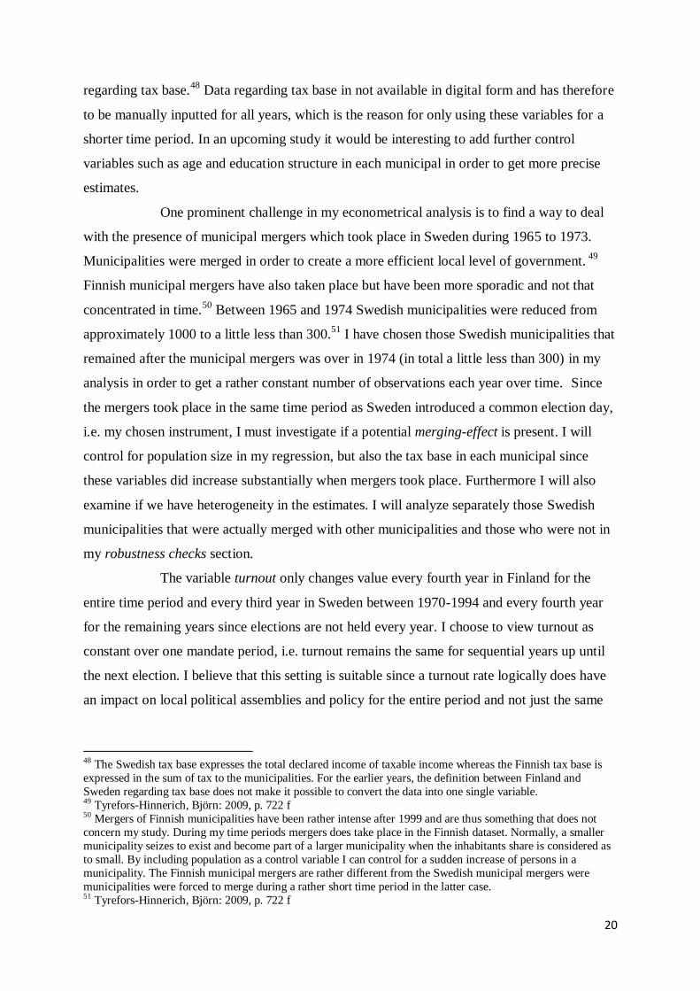
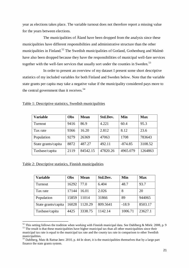
In order to present an overview of my dataset I present some short descriptive

statistics of my included variables for both Finland and Sweden below. Note that the variable

state grants per capita may take a negative value if the municipality considered pays more to

the central government than it receives.54

Table 1: Descriptive statistics, Swedish municipalities

Variable Obs Mean Std.Dev. Min Max

Turnout 9416 86.9 4.221 60.4 95.3

Tax rate 9366 16.20 2.812 8.12 23.6

Population 9279 26369 47063 1708 783643

State grants/capita 8872 487.27 492.11 -874.85 3108.52

Taxbase/capita 2119 84542.15 47820.26 4965.079 1264863

Table 2: Descriptive statistics, Finnish municipalities

Variable Obs Mean Std.Dev. Min Max

Turnout 16292 77.0 6.404 48.7 93.7

Tax rate 17144 16.01 2.026 8 20

Population 15859 11014 31866 89 944065

State grants/capita 16028 1120.29 809.5641 -18.9 8503.17

Taxbase/capita 4425 3338.75 1142.14 1006.71 23627.1

52 This setting follows the tradition when working with Finnish municipal data. See Dahlberg & Mörk: 2008, p. 9 53 The result is that these municipalities have higher municipal tax than all other municipalities since their

municipal tax rate is equal to the municipal tax rate and the county tax rate in comparison to other Swedish

municipalities. 54

Dahlberg, Matz & Rattsø Jørn: 2010, p. 44 In short, it is the municipalities themselves that by a large part

finance the state grants system.

22

4. Econometric model

Regarding the testing of the stipulated hypothesis, namely if a variation in turnout will affect

municipal tax rate, we have a potential problem with two-way causality. Just as turnout might

influence the local tax rate; a high tax rate might get people to vote in order to elect politicians

that lower the tax burden. Two-way causality is a threat against the internal validity and

implies that the regressor of interest is correlated with the error term. The result is inconsistent

estimates as a result of endogeneity in the model.55

As a solution to the endogeneity problem, an IV-approach will be applied where

the reform in Sweden in 1970 will be used as the instrument. Turnout is thus assumed to be a

function of the voting system. This is in line with my previous discussion, which is the

standard rational choice view that turnout will decrease when the cost associated with voting

has increased and vice versa. The calculation of the first stage in the IV-regression model

consequently answers the question if the introduction of a common election day in fact

imposed a higher turnout in Sweden. The first-stage regression is also important in order to

test if my chosen instrument is strong or if I have weak-instrument problem. The regression

equations are the following:

(11)

, 0 1 , 2 , ,i t i t i t t i i tTurnout Z W f v (12)

Β0 is the intercept. Xi,t is the variable of interest which is turnout in local elections in Finland

and Sweden. Wi,t is the vector of control variables. I will be using a panel data set and time

fixed effects, τt, and municipal fixed effects, fi, will be included. ui,t is the error term.

Equation (12) is the first-stage regression equation of (11). π0 is the intercept and Zi,t the

instrument, which is a binary variable taking the value 1 if the observation belongs to the

treatment group (Sweden) and the post treatment period (the year 1970 or later) and 0

otherwise. vi,t is the error term in the first stage equation. The same vector of control variables

will be included in the first-stage regression as well as time and municipal fixed effects. The

idea is to isolate the part of the variation in Xi, t that do not depend on the influence of the

dependent variable on Xi,t . The instrumental variable Zi,t thus isolate the part of Xi,t which is

uncorrelated with ui,t in order to get consistent estimates in (11).

55 Stock, James & Watson, Mark: 2007, p. 422

23

The testing of the reduced form, that is if there is any empirical evidence that

policy outcome differ between a system with a separate election days and a system with a

common election day will take the form of a difference-in-difference (DiD) analysis.

The Swedish municipalities will constitute the treatment group and the Finnish counterparts

the control group. A DiD approach is very suitable in this case in order to investigate the

causal effect of treatment. The regression function can be specified as:

, 0 1 2 3 4 , ,Tax rate ( * )i t t i t i i t t i i tP T P T W f u

(13)

β0 is the intercept. Ti is a binary variable taking the value 1 if the observation

belongs to the treatment group (Sweden) and 0 if belonging to the control group (Finland). Pt

is a binary variable taking the value 1 if the observation belongs to the treatment period or 0

otherwise. The same vector of control variables, Wi,t , will be included in order to compensate

for potential difference between the treatment group and the control group as well as

municipal and time fixed effects. ui,t is the error term. One may think of the reduced form as

the first stage multiplied by the second stage in the IV-regression thus saying something about

the economical significance of the estimated coefficients.

One important reason to estimate the reduced form, is to investigate if there is a

potential lag in the political system. Three separate treatment period, Pt, will as a result be

created. The first treatment period variable takes the value 1 if the observation belongs to the

year 1970, 1971, 1972 or 1973 and 0 otherwise. The second treatment period variable takes

the value 1 if the observation belongs to the year 1974, 1975, 1976, 1977, 1978 or 1979 and 0

otherwise. Lastly, the third treatment period variable takes the value 1 if the observation

belongs and any year after 1980 and 0 otherwise. The variables of interests are the interaction

variables (Pt*Ti) – which will be three in total – thus taking the value 1 if the observation

both belongs to the treatment group and one of the treatment periods above mentioned. The

estimation of parameter β3 measures consequently the causal effect of changing from a voting

system with separate election days into a system with one common election day.

In total, three different time periods will be considered in my empirical analysis:

1964-1973, 1964-1979 and 1964-1999. This yields for both the IV-analysis as well as the

DiD-analysis. All three of the above mentioned interaction variables will be included in the

DiD-analysis when the longest time period is considered, the first two in the 1964-1979 time

period and just the first in the shortest 1964-1973 time period. The reason for choosing the

24

time period 1964-1973 is because 1973 is an election year in Sweden and the second election

with a common election day (the 1970 year election was the first). The longest time period,

1964-1999 will naturally be included since this constitutes the whole time span in my data.

The time period 1964-1979 have been chosen in order to have a time period between the

shortest and the longest; however the year of 1979 as the end year has no particular reason. I

wanted a time period which was close to the treatment in the year 1970, but not as close as

1973 and the year 1979 seemed suitable. By having separate time periods I may investigate if

the estimated effects are different when the time period is extended/shortened.

Both municipal fixed effects and time fixed effects will be included in all

performed regressions. By including municipal fixed effects I control for omitted variables

that might differ between municipalities but remain constant over time. The econometrical

interpretation is that I create a unique intercept for each municipality in the panel. The

inclusion of time fixed effects means that I control for omitted variables that vary over time

but remains constant between municipalities. A fixed effects approach is very suitable in my

case since there is most certainly some omitted variable bias present in my specified model.56

The identifying assumption behind IV-regression is that of instrument relevance

and exogeneity. Relevance implies that the instrument must affect the endogenous regressor,

i.e. they must be correlated. By presenting first-stage regression outcome I can easily test if

this identifying assumption is fulfilled. Exogeneity implies that there cannot be any

correlation between the error term in the second stage regression and the instrument in the

first stage regression. If there is a correlation this means that the instrument directly affects

the outcome variable without any intermediate step.57

The analysis of the reduced forms gives

the causal effect of treatment on policy outcome; however I assume that the estimated effect

observed in this regression is due to a variation in turnout, which is then the intermediate step.

Unfortunately there is no direct way to test for exogeneity; one must simply argue that the

instrument does not affect the dependent variable directly. This thesis has a solid theoretical

base where turnout is seen as the intermediate step which will be affected when the voting

system is changed. Based on this theoretical foundation it does not seem likely that a change

in the voting system directly changes municipal tax rate without any intermediate step.

56 Stock, James & Watson, Mark: 2011, p. 396 f, 411. The reader should however note that these fixed effects

cannot control for characteristics that fluctuate both between municipalities and over time. 57 Stock, James & Watson, Mark 2007, p. 439 ff

25

A difference-in-difference approach rests on the identifying assumption that

there should be no systematic difference in the trend in the outcome variable between the

treatment group and the control group. This can also be translated as the two groups should be

very similar to each other.58

In order to argue that Finland and Sweden constitute suitable

testing ground for the purpose at hand in this thesis, the next section contains proof that

Sweden and Finland greatly resemble each other.

There is other obstacles associated with DiD-analysis. In Bertrand et al (2004)

the authors ask the question if we can trust difference-in-difference estimates. According to

Bertrand et al (2004), the standard errors calculated in a panel OLS-regression, which is the

estimation procedure often used in DiD-analysis, may be understated with the result of false

statistical significance meaning that there is possibly not a statistical significant effect of

treatment on the dependent variable. The reason for this is serial correlation in the dependent

variable. Clustering the standard errors is one potential solution where one allows for

autocorrelation in the error terms over time. Standard errors may then be correlated within a

cluster but not between different clusters. This is however problematic in my case since I only

use municipal data from two different countries. Bertrand et al (2004) suggest that one can

collapse the data into pre treatment and post treatment periods. Another solution often

discussed lately is to run the difference-in-difference regression in two stages. The first stage

is a regression with all the control variables as independent variables and the dependent

variable. Then one extracts the variation in the residual which is assumed to contain the

variation of the treatment variable and uses this to run the second stake regression. 59

There is

an ongoing debate among economists and econometricians which procedure to use. In this

master’s thesis I do not choose to pursue these econometric techniques; however in an

upcoming study this is a problem which need to be addressed.

5. Institutional background

The empirical strategy in this thesis rests on the assumption that Finland and Sweden are two

very comparable countries with similar political institutions, especially when it comes to the

institutional setting of Swedish and Finnish municipalities.

Every third or fourth year, general elections are held to the municipal councils in

Swedish and Finnish municipalities. Local political parties are not uncommon; however the

58

Stock, James & Watson, Mark: 2007, p. 480 ff 59 Bertrand et al: 2004, p. 250 f, 273 f

26

parties represented in the Swedish and Finnish parliaments are the dominant parties also on

the local level. 60

According to Dahlberg & Mörk (2011) the municipalities in Sweden and

Finland are interesting study objects since they have a high degree of regulated autonomy vis

à vis the central government. They are also important and powerful economic entities

operating in a very similar macroeconomic environment. The Swedish municipalities are

responsible for the supply of welfare services such as elderly care, childcare, social assistance,

primary as well as secondary education.61

The municipalities are also important employers. At

present date, there are 290 municipalities in Sweden. 62

There is great resemblance between

Sweden and Finland when it comes to the statue of the local government. The Finish

municipalities, 432 in total in the end of 1999, have the same rights and responsibilities as

their Swedish counterparts. In addition, they do often have the responsibility of health care.

Regarding income, both the Swedish and Finnish municipalities collect an income tax and

they freely regulate the level of it. The municipal tax constitutes the main source of income

for both Swedish and Finnish municipalities. Municipalities in both countries have the legal

right to borrow money on the financial market. In addition, they receive grants from the

central level of government in a various degree based on the idea of redistribution between

rich and poor municipalities. Before 1993, grants were typically targeted grants as the elected

local officials merely implemented different initiatives financed by the central government.

During 1993, both Finland and Sweden underwent important grant reforms where the goal

was to enhance the influence of local government. After 1993, grants have in a greater extent

been general. 63

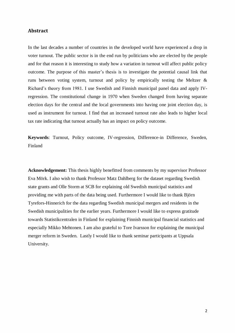
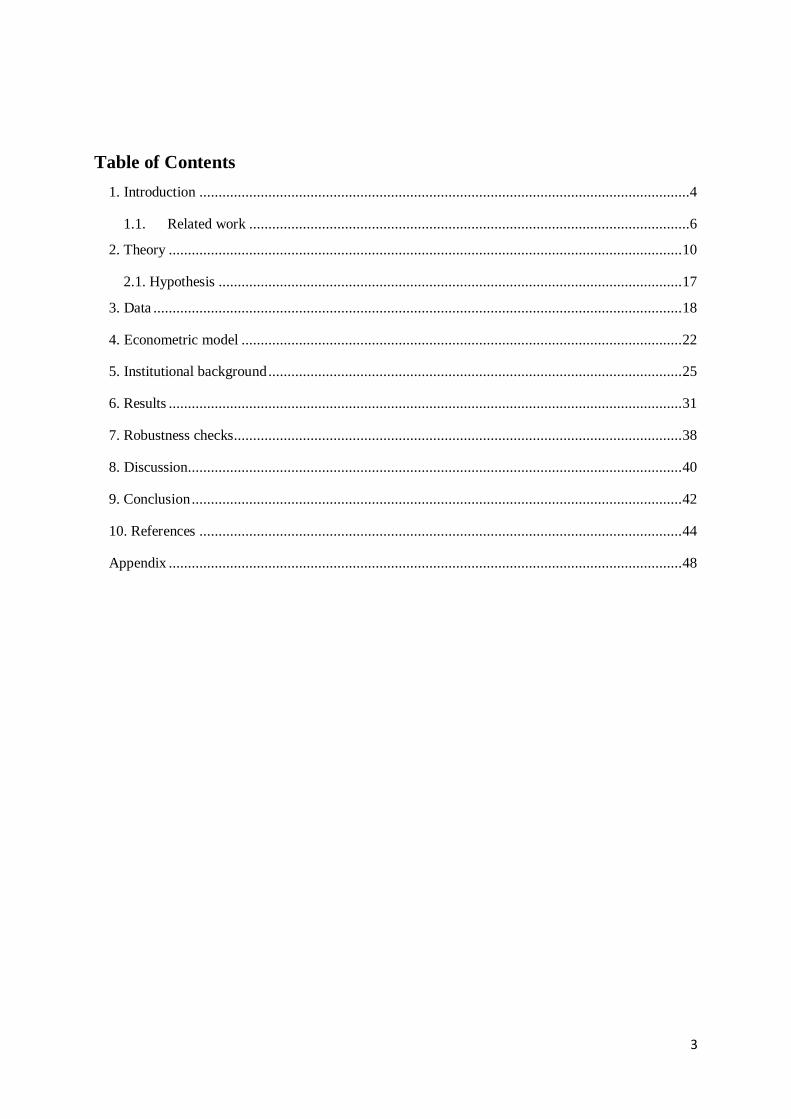
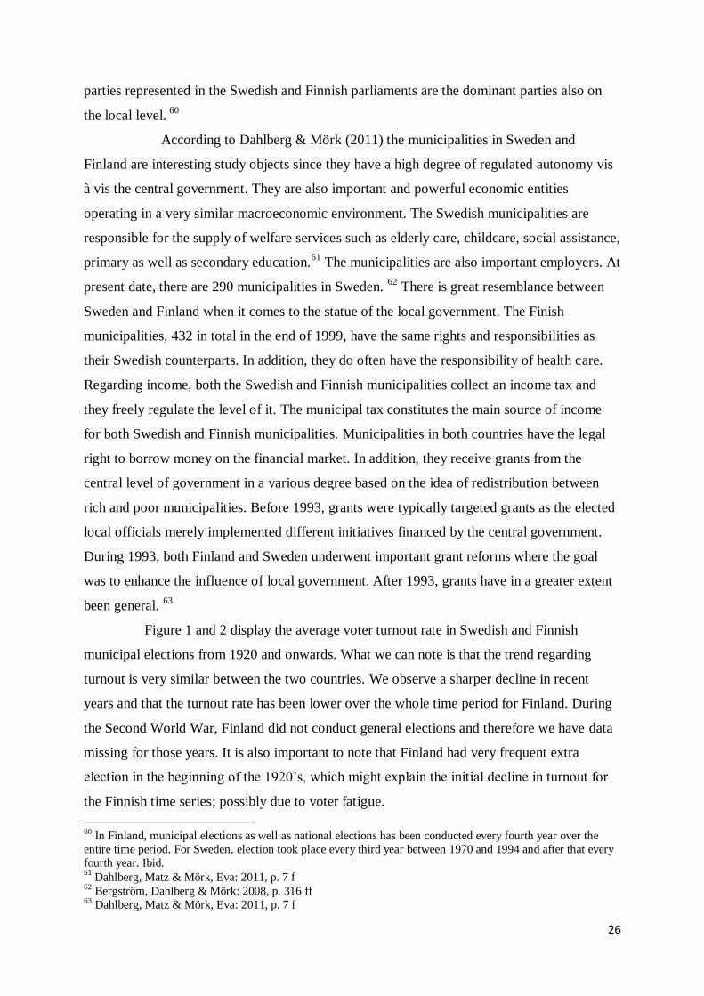
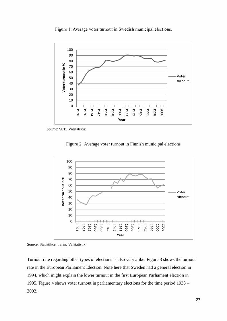
Figure 1 and 2 display the average voter turnout rate in Swedish and Finnish

municipal elections from 1920 and onwards. What we can note is that the trend regarding

turnout is very similar between the two countries. We observe a sharper decline in recent

years and that the turnout rate has been lower over the whole time period for Finland. During

the Second World War, Finland did not conduct general elections and therefore we have data

missing for those years. It is also important to note that Finland had very frequent extra

election in the beginning of the 1920’s, which might explain the initial decline in turnout for

the Finnish time series; possibly due to voter fatigue.

60 In Finland, municipal elections as well as national elections has been conducted every fourth year over the

entire time period. For Sweden, election took place every third year between 1970 and 1994 and after that every

fourth year. Ibid. 61

Dahlberg, Matz & Mörk, Eva: 2011, p. 7 f 62

Bergström, Dahlberg & Mörk: 2008, p. 316 ff 63 Dahlberg, Matz & Mörk, Eva: 2011, p. 7 f

27

Figure 1: Average voter turnout in Swedish municipal elections.

Source: SCB, Valstatistik

Figure 2: Average voter turnout in Finnish municipal elections

Source: Statistikcentralen, Valstatistik

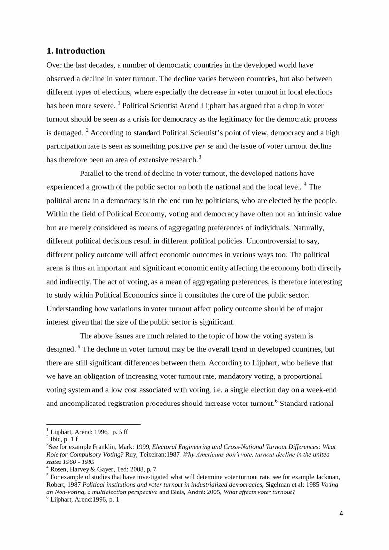
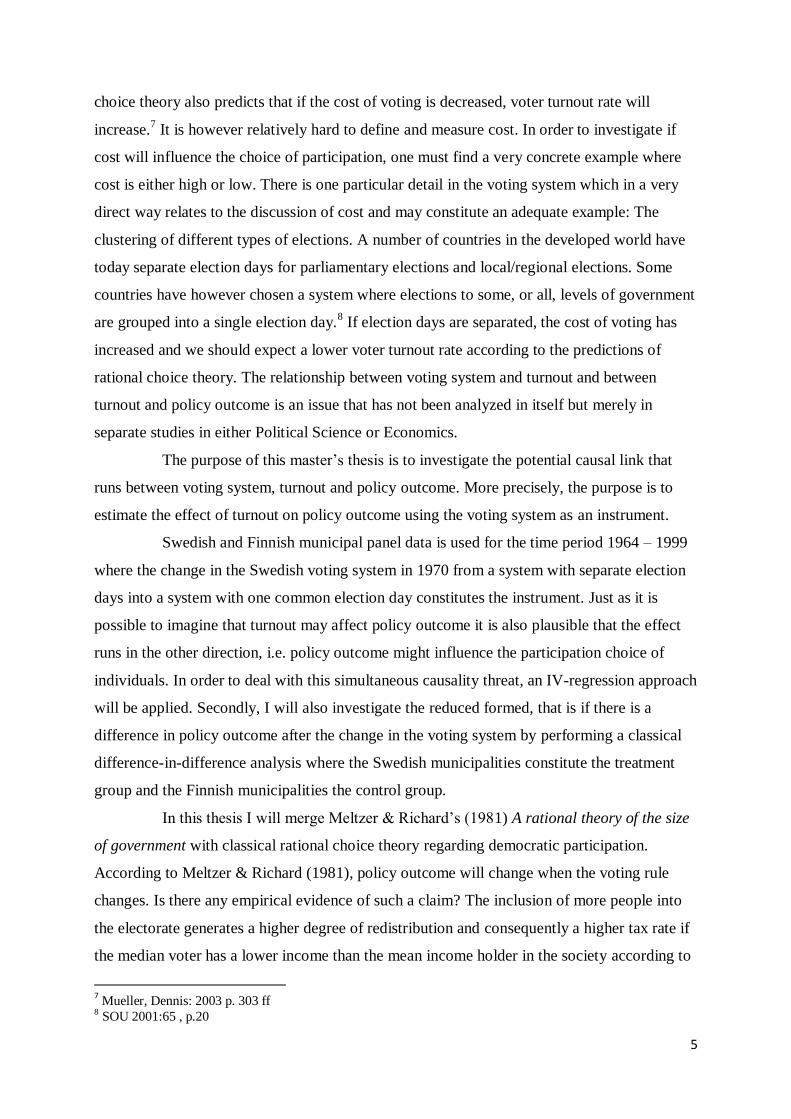
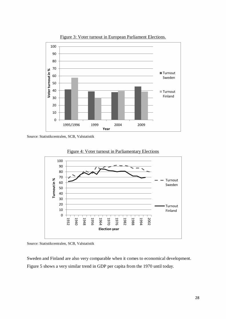
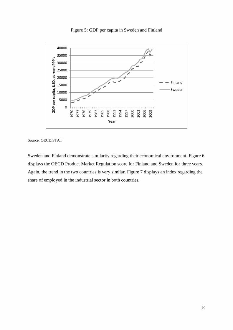
Turnout rate regarding other types of elections is also very alike. Figure 3 shows the turnout

rate in the European Parliament Election. Note here that Sweden had a general election in

1994, which might explain the lower turnout in the first European Parliament election in

1995. Figure 4 shows voter turnout in parliamentary elections for the time period 1933 –

2002.

0

10

20

30

40

50

60

70

80

90

100

1920

1926

1934

1942

1950

1958

1966

1973

1979

1985

1991

1998

2006V

ote

r tu

rno

ut i

n %

Year

Voterturnout

0

10

20

30

40

50

60

70

80

90

100

1921

1923

1925

1930

1936

1942

1947

1953

1960

1968

1976

1984

1992

2000

2008V

ote

r tu

rno

ut i

n %

Year

Voterturnout

28

Figure 3: Voter turnout in European Parliament Elections.

Source: Statistikcentralen, SCB, Valstatistik

Figure 4: Voter turnout in Parliamentary Elections

Source: Statistikcentralen, SCB, Valstatistik

Sweden and Finland are also very comparable when it comes to economical development.

Figure 5 shows a very similar trend in GDP per capita from the 1970 until today.

0

10

20

30

40

50

60

70

80

90

100

1995/1996 1999 2004 2009

Vo

ter

turn

ou

t in

%

Year

TurnoutSweden

TurnoutFinland

0

10

20

30

40

50

60

70

80

90

1001932

1940

1948

1956

1964

1970

1976

1982

1988

1994

2002

Turn

ou

t in

%

Election year

TurnoutSweden

TurnoutFinland

29

Figure 5: GDP per capita in Sweden and Finland

Source: OECD.STAT

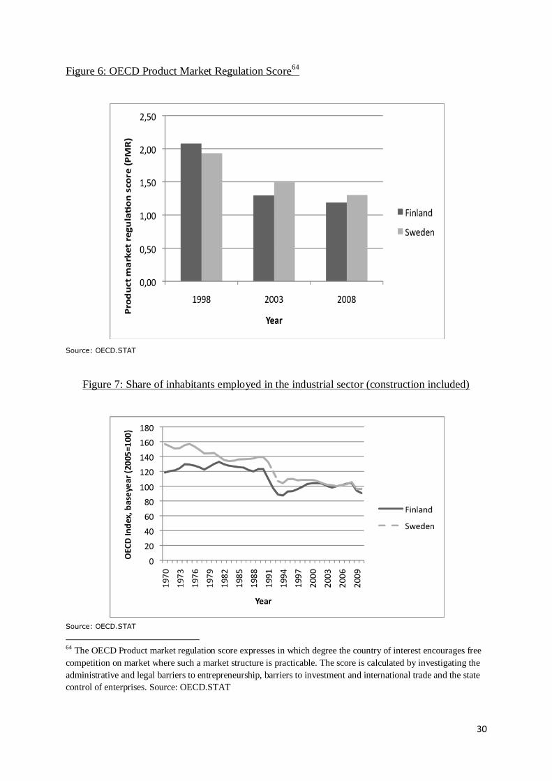
Sweden and Finland demonstrate similarity regarding their economical environment. Figure 6

displays the OECD Product Market Regulation score for Finland and Sweden for three years.

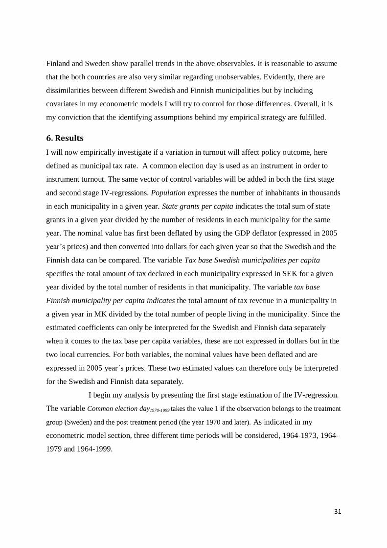
Again, the trend in the two countries is very similar. Figure 7 displays an index regarding the

share of employed in the industrial sector in both countries.

0

5000

10000

15000

20000

25000

30000

35000

40000

1970

1973

1976

1979

1982

1985

1988

1991

1994

1997

2000

2003

2006

2009G

DP

pe

r ca

pit

a, U

SD, c

urr

en

t P

PP

's

Year

Finland

Sweden

30

Figure 6: OECD Product Market Regulation Score64

Source: OECD.STAT

Figure 7: Share of inhabitants employed in the industrial sector (construction included)

Source: OECD.STAT

64 The OECD Product market regulation score expresses in which degree the country of interest encourages free

competition on market where such a market structure is practicable. The score is calculated by investigating the

administrative and legal barriers to entrepreneurship, barriers to investment and international trade and the state

control of enterprises. Source: OECD.STAT

31

Finland and Sweden show parallel trends in the above observables. It is reasonable to assume

that the both countries are also very similar regarding unobservables. Evidently, there are

dissimilarities between different Swedish and Finnish municipalities but by including

covariates in my econometric models I will try to control for those differences. Overall, it is

my conviction that the identifying assumptions behind my empirical strategy are fulfilled.

6. Results

I will now empirically investigate if a variation in turnout will affect policy outcome, here

defined as municipal tax rate. A common election day is used as an instrument in order to

instrument turnout. The same vector of control variables will be added in both the first stage

and second stage IV-regressions. Population expresses the number of inhabitants in thousands

in each municipality in a given year. State grants per capita indicates the total sum of state

grants in a given year divided by the number of residents in each municipality for the same

year. The nominal value has first been deflated by using the GDP deflator (expressed in 2005

year’s prices) and then converted into dollars for each given year so that the Swedish and the

Finnish data can be compared. The variable Tax base Swedish municipalities per capita

specifies the total amount of tax declared in each municipality expressed in SEK for a given

year divided by the total number of residents in that municipality. The variable tax base

Finnish municipality per capita indicates the total amount of tax revenue in a municipality in

a given year in MK divided by the total number of people living in the municipality. Since the

estimated coefficients can only be interpreted for the Swedish and Finnish data separately

when it comes to the tax base per capita variables, these are not expressed in dollars but in the

two local currencies. For both variables, the nominal values have been deflated and are

expressed in 2005 year´s prices. These two estimated values can therefore only be interpreted

for the Swedish and Finnish data separately.

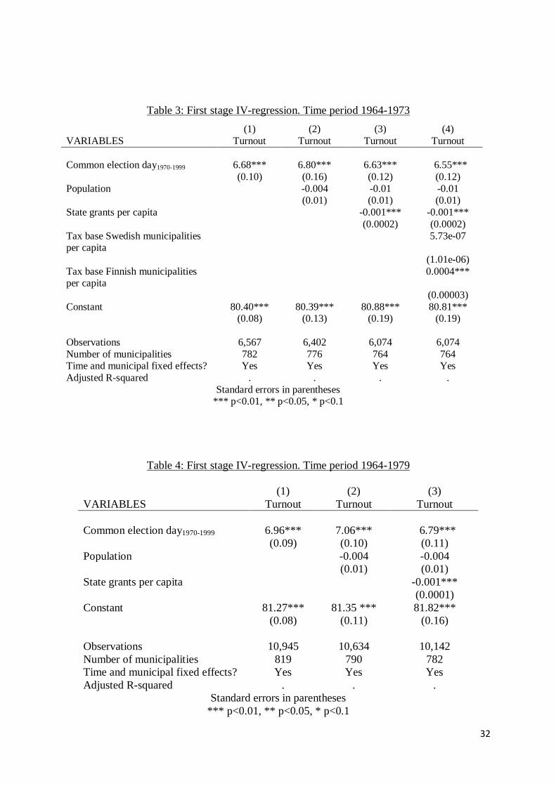
I begin my analysis by presenting the first stage estimation of the IV-regression.

The variable Common election day1970-1999 takes the value 1 if the observation belongs to the treatment

group (Sweden) and the post treatment period (the year 1970 and later). As indicated in my

econometric model section, three different time periods will be considered, 1964-1973, 1964-

1979 and 1964-1999.

32

Table 3: First stage IV-regression. Time period 1964-1973

(1) (2) (3) (4)

VARIABLES Turnout Turnout Turnout Turnout

Common election day1970-1999 6.68*** 6.80*** 6.63*** 6.55***

(0.10) (0.16) (0.12) (0.12)

Population -0.004 -0.01 -0.01 (0.01) (0.01) (0.01)

State grants per capita -0.001*** -0.001***

(0.0002) (0.0002)

Tax base Swedish municipalities per capita

5.73e-07

(1.01e-06)

Tax base Finnish municipalities per capita

0.0004***

(0.00003)

Constant 80.40*** 80.39*** 80.88*** 80.81*** (0.08) (0.13) (0.19) (0.19)

Observations 6,567 6,402 6,074 6,074

Number of municipalities 782 776 764 764 Time and municipal fixed effects? Yes Yes Yes Yes

Adjusted R-squared . . . .

Standard errors in parentheses *** p<0.01, ** p<0.05, * p<0.1

Table 4: First stage IV-regression. Time period 1964-1979

(1) (2) (3)

VARIABLES Turnout Turnout Turnout

Common election day1970-1999 6.96*** 7.06*** 6.79***

(0.09) (0.10) (0.11)

Population -0.004 -0.004

(0.01) (0.01)

State grants per capita -0.001***

(0.0001)

Constant 81.27*** 81.35 *** 81.82***

(0.08) (0.11) (0.16)

Observations 10,945 10,634 10,142

Number of municipalities 819 790 782

Time and municipal fixed effects? Yes Yes Yes

Adjusted R-squared . . .

Standard errors in parentheses

*** p<0.01, ** p<0.05, * p<0.1

33

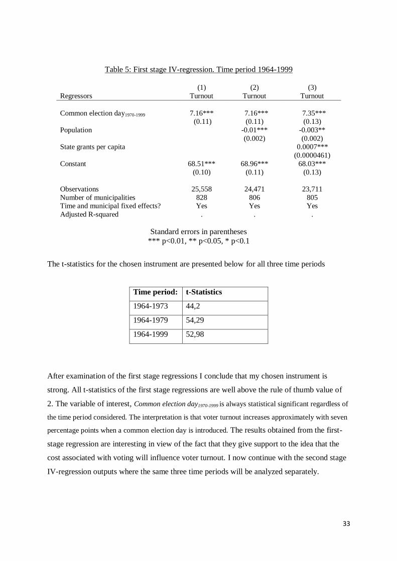
Table 5: First stage IV-regression. Time period 1964-1999

(1) (2) (3)

Regressors Turnout Turnout Turnout

Common election day1970-1999 7.16*** 7.16*** 7.35*** (0.11) (0.11) (0.13)

Population -0.01*** -0.003**

(0.002) (0.002) State grants per capita 0.0007***

(0.0000461)

Constant 68.51*** 68.96*** 68.03***

(0.10) (0.11) (0.13)

Observations 25,558 24,471 23,711

Number of municipalities 828 806 805 Time and municipal fixed effects? Yes Yes Yes

Adjusted R-squared

. . .

Standard errors in parentheses

*** p<0.01, ** p<0.05, * p<0.1

The t-statistics for the chosen instrument are presented below for all three time periods

Time period: t-Statistics

1964-1973 44,2

1964-1979 54,29

1964-1999 52,98

After examination of the first stage regressions I conclude that my chosen instrument is

strong. All t-statistics of the first stage regressions are well above the rule of thumb value of

2. The variable of interest, Common election day1970-1999 is always statistical significant regardless of

the time period considered. The interpretation is that voter turnout increases approximately with seven

percentage points when a common election day is introduced. The results obtained from the first-

stage regression are interesting in view of the fact that they give support to the idea that the

cost associated with voting will influence voter turnout. I now continue with the second stage

IV-regression outputs where the same three time periods will be analyzed separately.

34

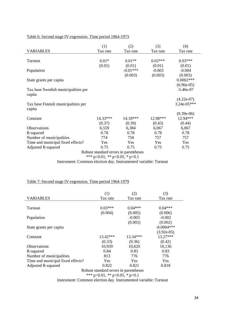
Table 6: Second stage IV-regression. Time period 1964-1973

(1) (2) (3) (4)

VARIABLES Tax rate Tax rate Tax rate Tax rate

Turnout 0.01* 0.01** 0.02*** 0.03***

(0.01) (0.01) (0.01) (0.01)

Population -0.01*** -0.003 -0.004 (0.003) (0.003) (0.003)

State grants per capita 0.0002***

(6.96e-05) Tax base Swedish municipalities per

capita

-5.46e-07

(4.22e-07)

Tax base Finnish municipalities per capita

3.24e-05***

(9.39e-06)

Constant 14.33*** 14.18*** 12.98*** 12.94*** (0.37) (0.39) (0.43) (0.44)

Observations 6,559 6,384 6,067 6,067

R-squared 0.78 0.78 0.78 0.78

Number of municipalities 774 758 757 757 Time and municipal fixed effects? Yes Yes Yes Yes

Adjusted R-squared 0.75 0.75 0.75 0.75

Robust standard errors in parentheses *** p<0.01, ** p<0.05, * p<0.1

Instrument: Common election day. Instrumented variable: Turnout

Table 7: Second stage IV-regression. Time period 1964-1979

(1) (2) (3)

VARIABLES Tax rate Tax rate Tax rate

Turnout 0.03*** 0.04*** 0.04***

(0.004) (0.005) (0.006) Population -0.003 -0.002

(0.002) (0.002)

State grants per capita -0.0004***

(3.92e-05) Constant 13.42*** 13.34*** 13.27***

(0.33) (0.36) (0.42)

Observations 10,939 10,620 10,136 R-squared 0.84 0.83 0.83

Number of municipalities 813 776 776

Time and municipal fixed effects? Yes Yes Yes Adjusted R-squared 0.822 0.821 0.818

Robust standard errors in parentheses

*** p<0.01, ** p<0.05, * p<0.1

Instrument: Common election day. Instrumented variable: Turnout

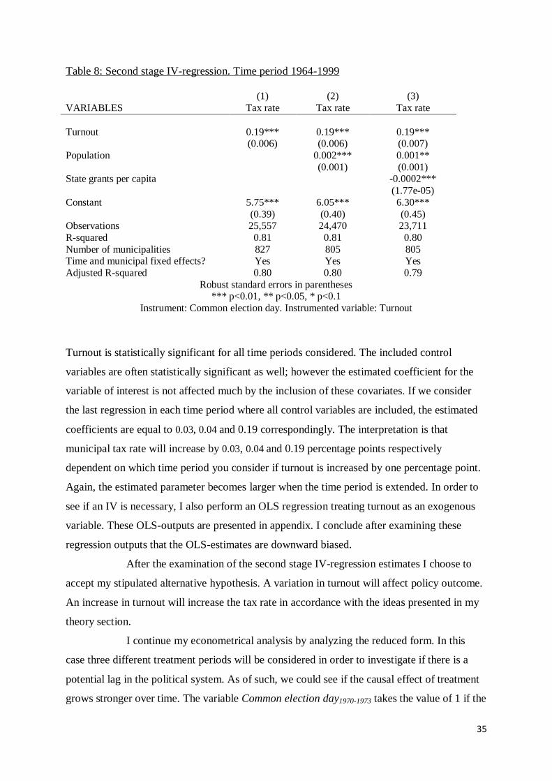
35

Table 8: Second stage IV-regression. Time period 1964-1999

(1) (2) (3)

VARIABLES Tax rate Tax rate Tax rate

Turnout 0.19*** 0.19*** 0.19*** (0.006) (0.006) (0.007)

Population 0.002*** 0.001**

(0.001) (0.001) State grants per capita -0.0002***

(1.77e-05)

Constant 5.75*** 6.05*** 6.30***

(0.39) (0.40) (0.45) Observations 25,557 24,470 23,711

R-squared 0.81 0.81 0.80

Number of municipalities 827 805 805 Time and municipal fixed effects? Yes Yes Yes

Adjusted R-squared 0.80 0.80 0.79

Robust standard errors in parentheses *** p<0.01, ** p<0.05, * p<0.1

Instrument: Common election day. Instrumented variable: Turnout

Turnout is statistically significant for all time periods considered. The included control

variables are often statistically significant as well; however the estimated coefficient for the

variable of interest is not affected much by the inclusion of these covariates. If we consider

the last regression in each time period where all control variables are included, the estimated

coefficients are equal to 0.03, 0.04 and 0.19 correspondingly. The interpretation is that

municipal tax rate will increase by 0.03, 0.04 and 0.19 percentage points respectively

dependent on which time period you consider if turnout is increased by one percentage point.

Again, the estimated parameter becomes larger when the time period is extended. In order to

see if an IV is necessary, I also perform an OLS regression treating turnout as an exogenous

variable. These OLS-outputs are presented in appendix. I conclude after examining these

regression outputs that the OLS-estimates are downward biased.

After the examination of the second stage IV-regression estimates I choose to

accept my stipulated alternative hypothesis. A variation in turnout will affect policy outcome.

An increase in turnout will increase the tax rate in accordance with the ideas presented in my

theory section.

I continue my econometrical analysis by analyzing the reduced form. In this

case three different treatment periods will be considered in order to investigate if there is a

potential lag in the political system. As of such, we could see if the causal effect of treatment

grows stronger over time. The variable Common election day1970-1973 takes the value of 1 if the

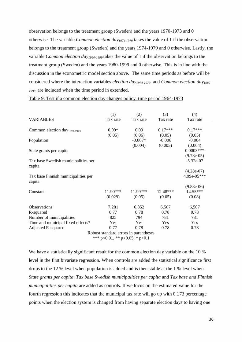
36

observation belongs to the treatment group (Sweden) and the years 1970-1973 and 0

otherwise. The variable Common election day1974-1979 takes the value of 1 if the observation

belongs to the treatment group (Sweden) and the years 1974-1979 and 0 otherwise. Lastly, the

variable Common election day1980-1999 takes the value of 1 if the observation belongs to the

treatment group (Sweden) and the years 1980-1999 and 0 otherwise. This is in line with the

discussion in the econometric model section above. The same time periods as before will be

considered where the interaction variables election day1974-1979 and Common election day1980-

1999 are included when the time period in extended.

Table 9: Test if a common election day changes policy, time period 1964-1973

(1) (2) (3) (4) VARIABLES Tax rate Tax rate Tax rate Tax rate

Common election day1970-1973 0.09* 0.09 0.17*** 0.17***

(0.05) (0.06) (0.05) (0.05) Population -0.007* -0.006 -0.004

(0.004) (0.005) (0.004)

State grants per capita 0.0003*** (9.78e-05)

Tax base Swedish municipalities per

capita

-5.32e-07

(4.28e-07)

Tax base Finnish municipalities per

capita

4.99e-05***

(9.88e-06) Constant 11.90*** 11.99*** 12.48*** 14.55***

(0.029) (0.05) (0.05) (0.08)

Observations 7,281 6,852 6,507 6,507

R-squared 0.77 0.78 0.78 0.78

Number of municipalities 825 794 781 781

Time and municipal fixed effects? Yes Yes Yes Yes Adjusted R-squared 0.77 0.78 0.78 0.78

Robust standard errors in parentheses

*** p<0.01, ** p<0.05, * p<0.1

We have a statistically significant result for the common election day variable on the 10 %

level in the first bivariate regression. When controls are added the statistical significance first

drops to the 12 % level when population is added and is then stable at the 1 % level when

State grants per capita, Tax base Swedish municipalities per capita and Tax base and Finnish

municipalities per capita are added as controls. If we focus on the estimated value for the

fourth regression this indicates that the municipal tax rate will go up with 0.173 percentage

points when the election system is changed from having separate election days to having one

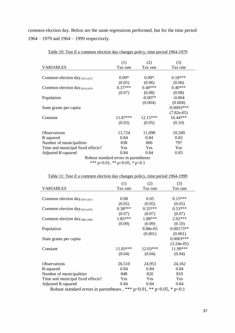
37

common election day. Below are the same regressions performed, but for the time period

1964 – 1979 and 1964 – 1999 respectively.

Table 10: Test if a common election day changes policy, time period 1964-1979

(1) (2) (3) VARIABLES Tax rate Tax rate Tax rate

Common election day1970-1973 0.09* 0.09* 0.18*** (0.05) (0.06) (0.06)

Common election day1974-1979 0.37*** 0.40*** 0.40***

(0.07) (0.08) (0.08)

Population -0.007* -0.004 (0.004) (0.004)

State grants per capita -0.0003***

(7.82e-05) Constant 11.87*** 12.15*** 16.44***

(0.03) (0.05) (0.10)

Observations 11,724 11,098 10,589 R-squared 0.84 0.84 0.83

Number of municipalities 838 806 797

Time and municipal fixed effects? Yes Yes Yes Adjusted R-squared 0.84 0.84 0.83

Robust standard errors in parentheses

*** p<0.01, ** p<0.05, * p<0.1

Table 11: Test if a common election day changes policy, time period 1964-1999

(1) (2) (3) VARIABLES Tax rate Tax rate Tax rate

Common election day1970-1973 0.08 0.05 0.15***

(0.05) (0.05) (0.05) Common election day1974-1979 0.38*** 0.35*** 0.53***

(0.07) (0.07) (0.07)

Common election day1980-1999 1.85*** 1.88*** 2.02*** (0.09) (0.09) (0.10)

Population 9.88e-05 0.00173**

(0.001) (0.001)

State grants per capita 0.0003*** (3.24e-05)

Constant 11.83*** 12.03*** 11.90***

(0.04) (0.04) (0.04)

Observations 26,510 24,953 24,162

R-squared 0.84 0.84 0.84

Number of municipalities 848 820 819 Time and municipal fixed effects? Yes Yes Yes

Adjusted R-squared 0.84 0.84 0.84

Robust standard errors in parentheses , *** p<0.01, ** p<0.05, * p<0.1

38

A very similar pattern manifests itself when the whole time period is considered. What we see

here is support for our previous suspicion, namely that there is a lag in the political system.

The estimated causal effect of treatment, that is introducing a common election day, becomes

larger when this is taken into consideration. The estimated coefficients for the variable

Common election day1970-1973 are rather similar between the three different time periods which

should be expected. If we focus on the longest time period analyzed in table 4 the variable

Common election day1970-1973 is only statistical significant on the 12 % level in the bivariate case

but becomes statistical significant on the 1 % level when all controls are added. The estimated

coefficient for the variable Common election day1970-1973 is equal to 0.15 is this case meaning

that the municipal tax rate will increase with 0.15 percentage points when a common election

day is introduced. However, the estimated parameters for variables Common election day1974-1979

and Common election day1980-1999 are 0.48 and 2.02 respectively when all controls are added

which indicates that the causal effect of treatment grows stronger over time. The last estimate

equal to 2.017 is large and might be questioned. Remember that the variable Common election

day1980-1999 takes the value of 1 of the observation belongs to any year after 1980 and the treatment

group (Sweden). 1980 is ten years after the actual treatment was implemented and the estimated value

equal to 2.02 might be due to other differences than just the change in the voting system. The problem

when one tries to take the lag in the political system into consideration is that one might consider a lag

that is to long which might be the case with this last estimate. The reduced form indicates that the

introduction of a common election day yields a higher municipal tax rate and the IV-analysis confirms

that turnout is the intermediate step between the change in the voting system and policy outcome. The

actual estimated values in the reduced form analysis must however be interpreted with caution where

the true effect on municipal tax rate of treatment is probably between the estimated coefficients of the

Common election day variables in the above analysis.

7. Robustness checks

In this section I will focus on two separate issues. First of all, I will address some of the

underlying assumptions behind regression in order to see if my results are robust. Secondly, I

will further investigate if the estimated effects are different when considering different

subsamples of the data.

One important underlying assumption behind regression is that the included

regressors are not highly correlated with each other. If they are, we have a problem with

multicollinearity which gives rise to inefficient estimates. In order to check for the presence

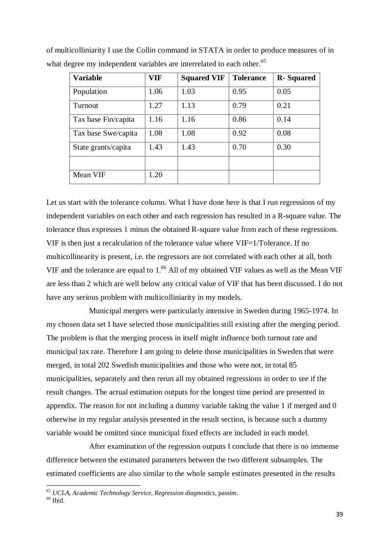
39

of multicolliniarity I use the Collin command in STATA in order to produce measures of in

what degree my independent variables are interrelated to each other.65

Variable VIF Squared VIF Tolerance R- Squared

Population 1.06 1.03 0.95 0.05

Turnout 1.27 1.13 0.79 0.21

Tax base Fin/capita 1.16 1.16 0.86 0.14

Tax base Swe/capita 1.08 1.08 0.92 0.08

State grants/capita 1.43 1.43 0.70 0.30

Mean VIF 1.20

Let us start with the tolerance column. What I have done here is that I run regressions of my

independent variables on each other and each regression has resulted in a R-square value. The

tolerance thus expresses 1 minus the obtained R-square value from each of these regressions.

VIF is then just a recalculation of the tolerance value where VIF=1/Tolerance. If no

multicollinearity is present, i.e. the regressors are not correlated with each other at all, both

VIF and the tolerance are equal to 1.66

All of my obtained VIF values as well as the Mean VIF

are less than 2 which are well below any critical value of VIF that has been discussed. I do not

have any serious problem with multicolliniarity in my models.

Municipal mergers were particularly intensive in Sweden during 1965-1974. In

my chosen data set I have selected those municipalities still existing after the merging period.

The problem is that the merging process in itself might influence both turnout rate and

municipal tax rate. Therefore I am going to delete those municipalities in Sweden that were

merged, in total 202 Swedish municipalities and those who were not, in total 85

municipalities, separately and then rerun all my obtained regressions in order to see if the

result changes. The actual estimation outputs for the longest time period are presented in

appendix. The reason for not including a dummy variable taking the value 1 if merged and 0

otherwise in my regular analysis presented in the result section, is because such a dummy

variable would be omitted since municipal fixed effects are included in each model.

After examination of the regression outputs I conclude that there is no immense

difference between the estimated parameters between the two different subsamples. The

estimated coefficients are also similar to the whole sample estimates presented in the results

65

UCLA, Academic Technology Service, Regression diagnostics, passim. 66 Ibid.

40

section. The statistical significance does not change, nor the direction of the point estimates.

The actual estimated coefficient varies slightly between the two groups where the estimated

effect is higher when only the Swedish municipalities that were not merged are included in

the analysis. I conclude that my obtained estimates in the result section are robust regarding

this specific issue.

8. Discussion

After performing the econometrical analysis I decide to accept my stipulated hypothesis given

that the obtained coefficients for the variable of interests are statistically significant when

both considering a short and a long time period and analyzing merged and not merged

municipalities separately. Equally important to discuss however, is the matter of economical

significance. Are the estimated effects large or are they to be considered as insignificant in

economical terms?

Turnout has an effect on the municipal tax level; nevertheless the effect vary

when different time periods are considered. If we consider the whole time period and focus on

the estimates when all covariates are included the municipal tax rate will increase by 0.19

percentage points when turnout increases by one percentage point. Suppose that turnout

increases by 10 percentage points which will then equal to a 1.9 percentage points increase in

municipal tax rate. Consider a yearly income of 300,000 SEK (25,000 per month), which

equal a yearly income of approximately 45,000 USD. 67

. An increase in turnout rate by 10

percentage points then equals a decrease of 5700 SEK or 855 USD in yearly income or 475

SEK/71 USD in monthly income. Or to be even more concrete: A 10 percentage points

decrease in turnout rate will give a middle income earner in Sweden and Finland the

possibility of having a fairly nice restaurant visit once per month. Is this effect considered to

be economically significant? It depends on what you compare with of course, however I

believe that 475 SEK/71 USD per month is not a gigantic amount of money, but is clearly

economically significant for the majority of the income earners. The mean tax rate for Sweden

and Finland was slightly larger than 16 percents for the entire time period. 1.9 percents equals

approximately 12 % of 16 percentage points. After analyzing the first stage regressions, I

concluded that turnout was increased by approximately 7 percentage points when introducing

a common election day in Sweden. This equals an increase in municipal tax rate by total 1.30

percentage points thus reducing the yearly income by roughly 3900 SEK/585 USD if the

67 The exchange rate considered is equal to 6.247. Source: Ekonomifakta.se

41

yearly income is 300,000 SEK/45,000 USD. Again, this is perhaps not an enormous amount

of money; however still economical significant.

The first stage regression is in my opinion very interesting. First of all, it gives

support to the rational choice theory that the cost associated with voting will influence the

choice of participation. Second of all, it has direct policy implications for Sweden. As already

noted, there is an ongoing debate in Sweden if the voting system should be changed in order

to implement separate election days to different levels of government. Given the results in this

study, such a reform would decrease voter turnout rate. Earlier Swedish official reports have

however claimed after performing before-and-after and cross-country analysis that turnout

rate will decrease in the rate 10 to 20 percentage points. 68

I believe that my DiD analysis is a

much more suitable approach were the conclusion is that turnout increases by approximately

7 percentage points when a common election day is introduced. If we consider Sweden, the

Social Democrats and the Left Party are pro a common election day and the Green party, The

Moderate Party (The Conservatives), The Christian Democrats and the Peoples Party

(classical Liberal party) are pro separate election days.69

If we should simplify the political

discussion, the leftist parties are often pro more redistribution and higher taxes and the right-

wing parties favor lower taxes and less redistribution. The result in my thesis suggests that a

common election day increases turnout which in turn increases the tax rate. The parties in

Sweden seem to favor the voting system that is in line with their ideological preferences.

Turnout as a phenomenon has so far not been a matter of particular interest in

the field of Political Economy which I believe is a setback. Political Scientists have in a

significant degree focused on turnout but given that they often have the perspective that

turnout in itself has an intrinsic value their focus has been on turnout in itself and not on

turnout as a factor that will affect policy. Lutz & Marsch (2007) concluded that a variation in

turnout will not affect political outcome. In their empirical analysis they do not find support

for the popular view that a lower turnout will benefit right-wing parties and disfavor left-wing

parties.70

This might be the case; on the other hand my study shows that a variation in turnout

will have an effect on policy outcome. One interpretation is in accordance with the Meltzer &

Richards (1981) theory that when turnout decreases, the median voter is no longer the same

person and this will in turn shift the whole political spectrum in another direction where all

parties propose policies in line with the new median voter in order to maximize their utility.

68 SOU 2001:65, p. 75 ff 69

Ibid, p. 55 70 Lutz, George & Marsch, Miachel: 2007, p. 1 ff

42

Turnout will in this case not just be something Political Scientists consider as good but also

something that will affect the economy of ordinary citizens. This thesis have made used of

municipal panel data from Sweden and Finland; however I believe that my study has a rather

high external validity. I have chosen my dataset since I believe there are good arguments for

using municipal panel data when investigating the relationship between turnout and policy

outcome. Since Swedish and Finnish municipalities are very alike, the true causal effect of a

variation in turnout is better estimated in such a dataset. Therefore, I believe that my results

may be generalized and is one of the first attempts to answer the broader question if turnout

will affect policy outcome.

In an upcoming study it would be interesting to investigate if other policy

outcome variables will be affected by a variation in voter turnout. Public expenditure is one

such variable. It is also possible to investigate if economic outcome will change. The idea is

that turnout will affect policy outcome which in turn will affect economic outcome. Economic

growth and unemployment are such variables that might be interesting to study further. In my

study I have included population, state grants and tax base as control variables and it would

certainly be fruitful to include a larger vector of covariates. Age structure and education

structure in each municipality are such variables that could benefit the analysis, in order to

obtain more exact estimates. Furthermore, it would be interesting to see if the effect of turnout

on policy outcome would be the same if the initial turnout level is lower, since both Sweden

and Finland has a rather high turnout rate.

9. Conclusion

The purpose in this study was to investigate the potential causal link that runs between voting

system, turnout and policy. Meltzer & Richard’s A rational theory of the size of government

constituted the theoretical core in the thesis where theory predicted that when the voting

system was changed from having separate election days to having one common election day

voter turnout will go up; especially in those socioeconomic groups that are assumed to have a

lower taste for voting. This will in turn affect policy outcome resulting in more redistribution

and higher taxes. I used Swedish and Finnish municipal data from 1964-1999 and made use of

the fact that the Swedish constitution was changed in 1970 and a common election day was

introduced. An IV-approach was applied in order to see if an increase in turnout will result in

higher taxes. I found that this was the case. The effect of turnout on municipal tax rate

increased if a longer time period was considered and is both statistically and economically

significant. A common election day was here used as an instrument in order to instrument the

43

potential endogenous variable turnout. A difference-in-difference approach was also applied

in order to investigate the reduced form, i.e. if the constitutional change modified policy

outcome where the Finnish municipalities was the control group and the Swedish

municipalities the treatment group. I found that municipal tax rate was affected by the

introduction of a common election day and that the causal effect grew stronger over time.

44

10. References

Bergström, Dahlberg & Mörk: 2008, The effects of grants and wages on municipal

labour demand, Labour Economics 11, 315-334

Bertrand et al: 2004, How much should we trust difference-in-difference estimates?

The Quarentely Jounal of Economics, 249-275

Blais, A: 2006, What affects voter turnout? Annual review of Political Science, 111-

125

Boix, Charles:1999, Setting the Rules of the Game: The Choice of Electoral Systems in

Advanced Democracies, The American Political Science Review, 609-624

Bolton, Roger: 2005 Habemas theory of communicative action and the theory of

social capital. Department of Economics, Williams college

Borjas, George: 2008, Labor Economics, fourth edition, McGraw Hill

Caplan, Bryan: 2007, The Myth of the rational voter – Why democracies choose bad

policies, Princeton University Press

Dahlberg, Matz & Rattsø, Jørn: 2010, Statliga bidrag till kommunerna– i princip och

praktik, ESO-rapport

Dahlberg, Matz & Mörk, Eva: 2011, Is there an election cycle in public employment?

Seperating time effects from election year effects, CESifo Economic Studies,

upcoming

Ekonomifakta, available at www.ekonomifakta.se cited 110530

Franklin, Mark: 1999, Electoral Engineering and Cross-National Turnout

Differences: What Role for Compulsory Voting, British Journal of Political Science,

205-216

45

Fumagalli, Eileen & Narciso, Gaia: 2008, Political institutions, voter turnout and

policy outcomes, Institut for international integration studies

Jackman, Robert, 1987 Political institutions and voter turnout in industrialized

democracies, The American Political Sciences Review, 405-424

Lijphart, Arend: 1996, Unequal participation, democracy’s unsolved dilemma,

American Political Science Review, 1-14

Lott, John & Kenny, Lawrence: 1999, Did Women’s Suffrage Change the Size and

Scope of Government?, Journal of Political Economy 1163-1198

Lutz, George & Marsch, Miachel: 2007, Introduction: Consequences of low turnout,

Electoral Studies, 624- 632

Meltzer, Allan & Richards, Scott: 1981, A rational theory of the size of government.

Journal of Political Economy, 914-927

Mueller, Dennis & Stratmann, Thomas: 2003, The economic effect of democratic

participation, Journal of Public Economics, 2129-2155

Mueller, Dennis: 2003, Public Choice III, Cambridge University Press

Persson, Torsten: 2002, How political institutions shape economic policy,

Econometrica, 883-905

Rosen, Harvey & Gayer, Ted: 2008, Public Finance, McGraw Hill

Ruy A, Teixeira: 1987, Why Americans don’t vote: Turnout Decline in the United

States, 1960-1984, Greenwood Press

Statistiska centralbyrån (SCB),

46

o Turnout Sweden 1973-1999, available at:

http://www.scb.se/Pages/List____292050.aspx cited 101222

o Tax rate Sweden 1973-1999, available at

http://www.scb.se/Pages/SubjectArea____11842.aspx cited 110101

o Kommunalvalen 1970, 1966

o Årsbok för Sveriges kommuner, 1966, 1967, 1968, 1969, 1970, 1971, 1972,

1973, 1974

Sigelman et al: 1985 Voting and Non-voting, a multielection perspective, American

Journal of Political Science, 749-765

SOU 2000:1, En uthållig demokrati, demokratiberedningens betänkande, available at

http://www.sweden.gov.se/content/1/c4/06/24/1c43643c.pdf

SOU 2001:65, Skilda valdagar och vårval, available at

http://www.sweden.gov.se/sb/d/108/a/60120

SOU 2008:125, En reformerad grundlag, available at

http://www.regeringen.se/sb/d/10025/a/117744

SOU 2007:84, Värdet av valdeltagande, available at

http://www.sweden.gov.se/content/1/c6/09/20/24/b9868a62.pdf

Statistikcentralen,

o Turnout Finland, available at http://www.stat.fi/til/vaa_sv.html cited 101229

o Kommunal finansstatistik Finland 1964, 1965, 1966, 1967, 1968, 1969, 1970,

1971, 1972, 1973 and 1974

o Kommunalvalen 1964, 1968, 1972

o Årsbok för Finland, 1964, 1965, 1966, 1967, 1968, 1969, 1970, 1971, 1972,

1973. 1974

o Val, kommunalval & Riksdagsval, beskrivning av statistik, available at

http://www.stat.fi/meta/til/kvaa_sv.html cited 110315

47

Stock, James & Watson, Mark: 2011, Introduction to econometrics, 3 edition, Pearson

Education

Stock, James & Watson, Mark: 2007, Introduction to econometrics 2 edition, Pearson

Education

Tyrefors-Hinnerich, Björn: 2009, Do merging local governments free ride on their

counterparts when facing boundary reform?, Journal of Public Economics, 721-728

OECD.STAT, statistical database

UCLA, Academic Technology Service, Regression diagnostics, available at:

http://www.ats.ucla.edu/stat/stata/webbooks/logistic/chapter3/statalog3.htm cited

110601

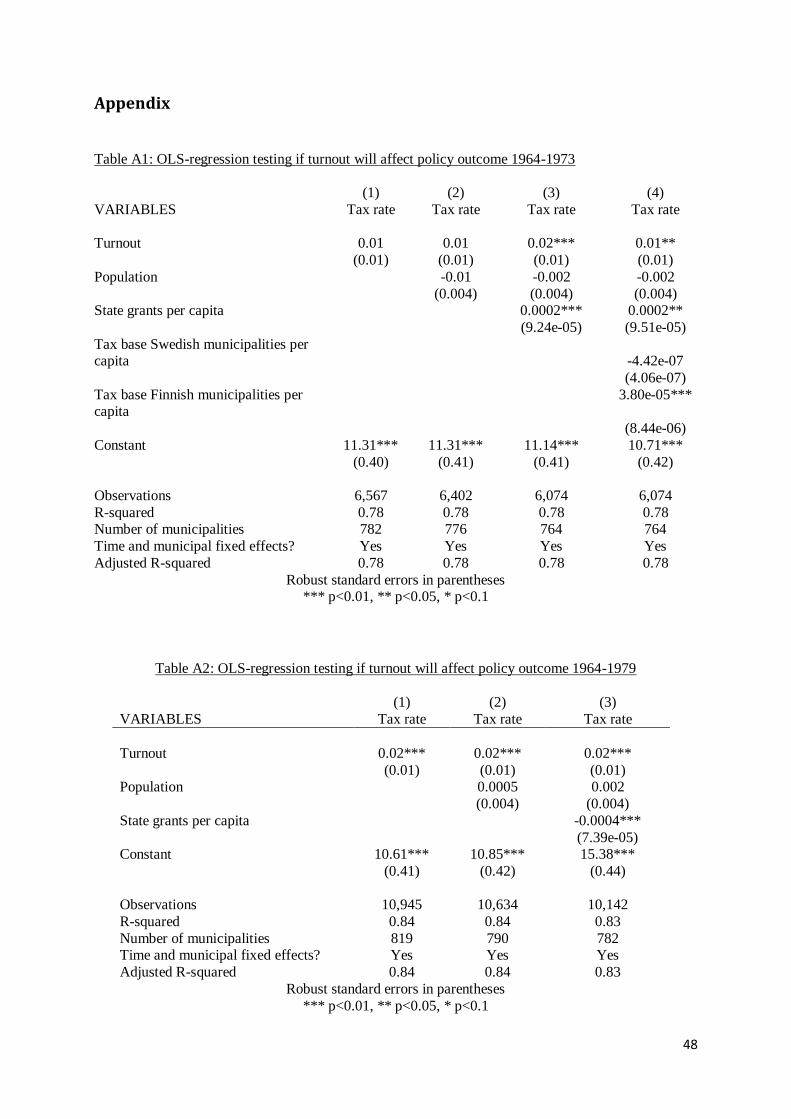
48

Appendix

Table A1: OLS-regression testing if turnout will affect policy outcome 1964-1973

(1) (2) (3) (4)

VARIABLES Tax rate Tax rate Tax rate Tax rate

Turnout 0.01 0.01 0.02*** 0.01**

(0.01) (0.01) (0.01) (0.01)

Population -0.01 -0.002 -0.002

(0.004) (0.004) (0.004) State grants per capita 0.0002*** 0.0002**

(9.24e-05) (9.51e-05)

Tax base Swedish municipalities per capita

-4.42e-07

(4.06e-07)

Tax base Finnish municipalities per capita

3.80e-05***

(8.44e-06)

Constant 11.31*** 11.31*** 11.14*** 10.71***

(0.40) (0.41) (0.41) (0.42)

Observations 6,567 6,402 6,074 6,074

R-squared 0.78 0.78 0.78 0.78 Number of municipalities 782 776 764 764

Time and municipal fixed effects? Yes Yes Yes Yes

Adjusted R-squared 0.78 0.78 0.78 0.78

Robust standard errors in parentheses *** p<0.01, ** p<0.05, * p<0.1

Table A2: OLS-regression testing if turnout will affect policy outcome 1964-1979

(1) (2) (3)

VARIABLES Tax rate Tax rate Tax rate

Turnout 0.02*** 0.02*** 0.02***

(0.01) (0.01) (0.01) Population 0.0005 0.002

(0.004) (0.004)

State grants per capita -0.0004***

(7.39e-05) Constant 10.61*** 10.85*** 15.38***

(0.41) (0.42) (0.44)

Observations 10,945 10,634 10,142

R-squared 0.84 0.84 0.83

Number of municipalities 819 790 782 Time and municipal fixed effects? Yes Yes Yes

Adjusted R-squared 0.84 0.84 0.83

Robust standard errors in parentheses

*** p<0.01, ** p<0.05, * p<0.1

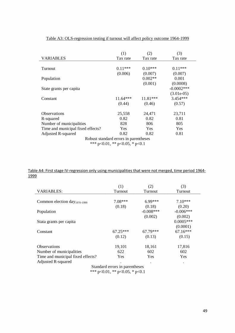
49

Table A3: OLS-regression testing if turnout will affect policy outcome 1964-1999

(1) (2) (3) VARIABLES Tax rate Tax rate Tax rate

Turnout 0.11*** 0.10*** 0.11***

(0.006) (0.007) (0.007) Population 0.002** 0.001

(0.001) (0.0008)

State grants per capita -0.0002*** (3.01e-05)

Constant 11.64*** 11.81*** 3.454***

(0.44) (0.46) (0.57)

Observations 25,558 24,471 23,711

R-squared 0.82 0.82 0.81

Number of municipalities 828 806 805 Time and municipal fixed effects? Yes Yes Yes

Adjusted R-squared 0.82 0.82 0.81

Robust standard errors in parentheses

*** p<0.01, ** p<0.05, * p<0.1

Table A4: First stage IV-regression only using municipalities that were not merged, time period 1964-1999

(1) (2) (3) VARIABLES: Turnout Turnout Turnout

Common election day1970-1999 7.08*** 6.99*** 7.10*** (0.18) (0.18) (0.20)

Population -0.008*** -0.006***

(0.002) (0.002)

Stata grants per capita 0.0005*** (0.0001)

Constant 67.25*** 67.79*** 67.16***

(0.12) (0.13) (0.15)

Observations 19,101 18,161 17,816

Number of municipalities 622 602 602 Time and municipal fixed effects? Yes Yes Yes

Adjusted R-squared . . .

Standard errors in parentheses

*** p<0.01, ** p<0.05, * p<0.1

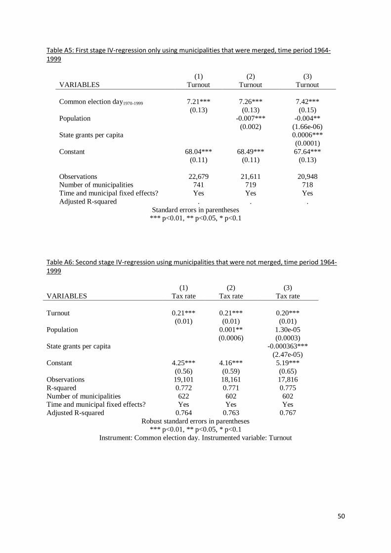
50

Table A5: First stage IV-regression only using municipalities that were merged, time period 1964-1999

(1) (2) (3)

VARIABLES Turnout Turnout Turnout

Common election day1970-1999 7.21*** 7.26*** 7.42***

(0.13) (0.13) (0.15)

Population -0.007*** -0.004**

(0.002) (1.66e-06) State grants per capita 0.0006***

(0.0001)

Constant 68.04*** 68.49*** 67.64*** (0.11) (0.11) (0.13)

Observations 22,679 21,611 20,948 Number of municipalities 741 719 718

Time and municipal fixed effects? Yes Yes Yes

Adjusted R-squared . . .

Standard errors in parentheses *** p<0.01, ** p<0.05, * p<0.1

Table A6: Second stage IV-regression using municipalities that were not merged, time period 1964-1999

(1) (2) (3)

VARIABLES Tax rate Tax rate Tax rate

Turnout 0.21*** 0.21*** 0.20*** (0.01) (0.01) (0.01)

Population 0.001** 1.30e-05

(0.0006) (0.0003) State grants per capita -0.000363***

(2.47e-05)

Constant 4.25*** 4.16*** 5.19***

(0.56) (0.59) (0.65) Observations 19,101 18,161 17,816

R-squared 0.772 0.771 0.775

Number of municipalities 622 602 602 Time and municipal fixed effects? Yes Yes Yes

Adjusted R-squared 0.764 0.763 0.767

Robust standard errors in parentheses *** p<0.01, ** p<0.05, * p<0.1

Instrument: Common election day. Instrumented variable: Turnout

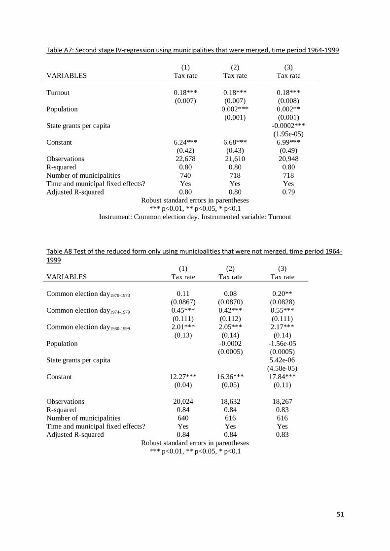
51

Table A7: Second stage IV-regression using municipalities that were merged, time period 1964-1999 (1) (2) (3)

VARIABLES Tax rate Tax rate Tax rate

Turnout 0.18*** 0.18*** 0.18*** (0.007) (0.007) (0.008)

Population 0.002*** 0.002**

(0.001) (0.001) State grants per capita -0.0002***

(1.95e-05)

Constant 6.24*** 6.68*** 6.99*** (0.42) (0.43) (0.49)

Observations 22,678 21,610 20,948

R-squared 0.80 0.80 0.80

Number of municipalities 740 718 718 Time and municipal fixed effects? Yes Yes Yes

Adjusted R-squared 0.80 0.80 0.79

Robust standard errors in parentheses *** p<0.01, ** p<0.05, * p<0.1

Instrument: Common election day. Instrumented variable: Turnout

Table A8 Test of the reduced form only using municipalities that were not merged, time period 1964-1999 (1) (2) (3)

VARIABLES Tax rate Tax rate Tax rate

Common election day1970-1973 0.11 0.08 0.20**

(0.0867) (0.0870) (0.0828)

Common election day1974-1979 0.45*** 0.42*** 0.55***

(0.111) (0.112) (0.111) Common election day1980-1999 2.01*** 2.05*** 2.17***

(0.13) (0.14) (0.14)

Population -0.0002 -1.56e-05 (0.0005) (0.0005)

State grants per capita 5.42e-06

(4.58e-05)

Constant 12.27*** 16.36*** 17.84*** (0.04) (0.05) (0.11)

Observations 20,024 18,632 18,267 R-squared 0.84 0.84 0.83

Number of municipalities 640 616 616

Time and municipal fixed effects? Yes Yes Yes Adjusted R-squared 0.84 0.84 0.83

Robust standard errors in parentheses

*** p<0.01, ** p<0.05, * p<0.1

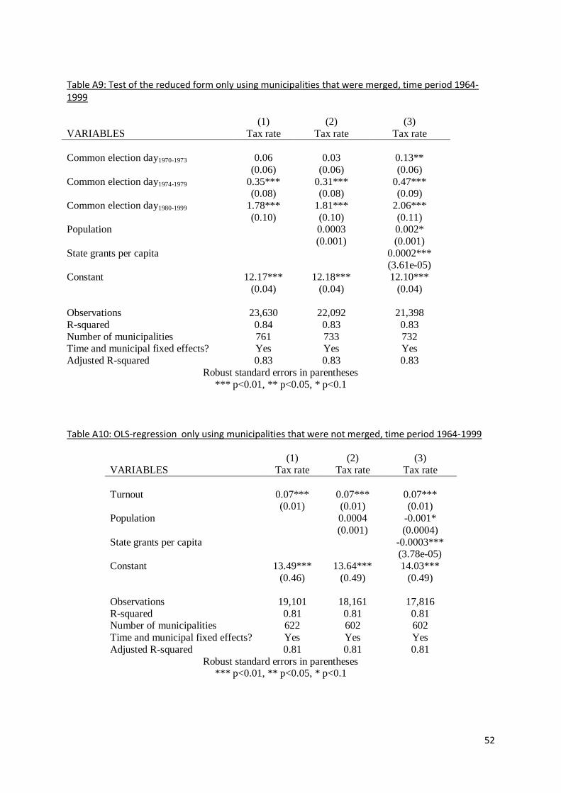
52

Table A9: Test of the reduced form only using municipalities that were merged, time period 1964-1999

(1) (2) (3)

VARIABLES Tax rate Tax rate Tax rate

Common election day1970-1973 0.06 0.03 0.13**

(0.06) (0.06) (0.06)

Common election day1974-1979 0.35*** 0.31*** 0.47*** (0.08) (0.08) (0.09)

Common election day1980-1999 1.78*** 1.81*** 2.06***

(0.10) (0.10) (0.11) Population 0.0003 0.002*

(0.001) (0.001)

State grants per capita 0.0002*** (3.61e-05)

Constant 12.17*** 12.18*** 12.10***

(0.04) (0.04) (0.04)

Observations 23,630 22,092 21,398

R-squared 0.84 0.83 0.83

Number of municipalities 761 733 732 Time and municipal fixed effects? Yes Yes Yes

Adjusted R-squared 0.83 0.83 0.83

Robust standard errors in parentheses

*** p<0.01, ** p<0.05, * p<0.1

Table A10: OLS-regression only using municipalities that were not merged, time period 1964-1999

(1) (2) (3)

VARIABLES Tax rate Tax rate Tax rate

Turnout 0.07*** 0.07*** 0.07*** (0.01) (0.01) (0.01)

Population 0.0004 -0.001*

(0.001) (0.0004)

State grants per capita -0.0003*** (3.78e-05)

Constant 13.49*** 13.64*** 14.03***

(0.46) (0.49) (0.49)

Observations 19,101 18,161 17,816

R-squared 0.81 0.81 0.81 Number of municipalities 622 602 602

Time and municipal fixed effects? Yes Yes Yes

Adjusted R-squared 0.81 0.81 0.81

Robust standard errors in parentheses *** p<0.01, ** p<0.05, * p<0.1

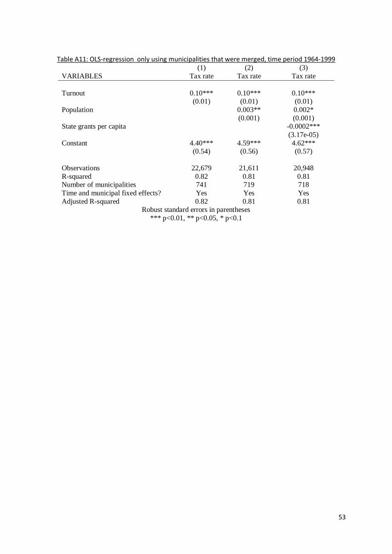
53

Table A11: OLS-regression only using municipalities that were merged, time period 1964-1999

(1) (2) (3)

VARIABLES Tax rate Tax rate Tax rate

Turnout 0.10*** 0.10*** 0.10*** (0.01) (0.01) (0.01)

Population 0.003** 0.002*

(0.001) (0.001) State grants per capita -0.0002***

(3.17e-05)

Constant 4.40*** 4.59*** 4.62*** (0.54) (0.56) (0.57)

Observations 22,679 21,611 20,948

R-squared 0.82 0.81 0.81 Number of municipalities 741 719 718

Time and municipal fixed effects? Yes Yes Yes

Adjusted R-squared 0.82 0.81 0.81 Robust standard errors in parentheses

*** p<0.01, ** p<0.05, * p<0.1