Embed Size (px)
Citation preview
VSC-HVDC based Network Reinforcement
Tamiru Woldeyesus Shire Student No: 1386042 M. Sc. Thesis Electrical power Engineering
Thesis supervisor: Prof.ir. L. van der Sluis (TUD)
Daily supervisors: Dr.ir. G. C. Paap (TUD), ir. R. L. Hendriks (TUD), ir. H. J. M. Arts ( STEDIN), P. Zonneveld ( STEDIN)
Delft University of Technology Faculty of Electrical Engineering, Mathematics and Computer Science
High-voltage Components and Power Systems (The work for this thesis has been carried out at STEDIN from October to May 2009) May 2009

i
Acknowledgement The research work is carried out at Network Solutions group, Asset Management division at STEDIN in conjunction with Delft University of Technology. First, I would like to express my deepest gratitude to my supervisors prof.ir. L. van der Sluis, dr.ir. G. C. Paap, ir. H. J. M. Arts, ir. R. L. Hendriks, and P. Zonneveld for there encouragement and guidance throughout the research work. Their readiness to help, patience and valuable suggestions were highly appreciated. I would also like to thank ir. E. J. Coster and dr.ir. A. M. van Voorden for the indispensable discussions we had throughout the thesis work. Last but not the least, I want to thank all Stedin B.V. employees for there kind cooperation.
ii
Contents Acknowledgement .........................................................................................................i
Chapter 1 Introduction..........................................................................................1 1.1 Introduction...........................................................................................................1 1.2 Problem Definition...............................................................................................1 1.3 Outline of the thesis ..............................................................................................2
Chapter 2 Network constraints and reinforcement ............................................4 2.1 Introduction...........................................................................................................4 2.2 Network model ......................................................................................................4 2.3 Network constraints..............................................................................................5 2.4 Network Reinforcement .......................................................................................6 2.5 HVDC transmission ..............................................................................................8
2.5.1 Arrangement of HVDC systems ...............................................................8 2.5.2 Classical HVDC Systems ...........................................................................9 2.5.3 Voltage source converter (VSC) HVDC system ....................................10
Chapter 3 Design and operating principle of VSC-HVDC ..............................13 3.1 Operating principle of VSC-HVDC ..................................................................13 3.2 Capability chart of VSC -HVDC .......................................................................14 3.3 PWM ....................................................................................................................15 3.4 VSC-HVDC station components .......................................................................15
3.4.1 Converters ................................................................................................15 3.4.2 Converter size...........................................................................................16 3.4.3 Converter transformer ............................................................................16 3.4.4 Direct voltage............................................................................................17 3.4.5 DC capacitor.............................................................................................17 3.4.6 Phase reactor ............................................................................................18 3.4.7 AC filters...................................................................................................19
Chapter 4 Control system of VSC-HVDC .........................................................21 4.1 Introduction.........................................................................................................21 4.2 Direct control.......................................................................................................21 4.3 Vector control......................................................................................................22
4.3.1 Inner Current controller .........................................................................25 4.3.1.1 PWM converter .................................................................................25 4.3.1.2 System transfer function ..................................................................26 4.3.1.3 Regulator ...........................................................................................27 4.3.1.4 Control block diagram .....................................................................27
4.3.2 Outer controllers ......................................................................................28 4.3.2.1 Direct voltage control .......................................................................28 4.3.2.2 Active and reactive power control...................................................30 4.3.2.3 Ac voltage control .............................................................................31
4.3.3 Limiting strategies ...................................................................................31 4.3.4 Controller integral windup .....................................................................32 4.3.5 Tuning of PI controllers ..........................................................................32
Chapter 5 Testing of VSC-HVDC model ...........................................................34 5.1 Introductions .......................................................................................................34
iii
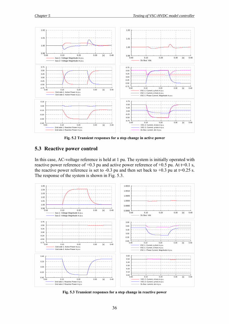
5.2 Active power control...........................................................................................35 5.3 Reactive power control .......................................................................................36 5.4 AC voltage control ..............................................................................................37 5.5 Three phase short circuit at Grid side-1 ...........................................................38 5.6 Unbalanced fault conditions: SLGF at Grid side-1 .........................................39 5.7 Three phase short circuit at Grid side-2 ...........................................................40 Conclusion ..................................................................................................................42
Chapter 6 Simulation Results .............................................................................43 6.1 Introduction.........................................................................................................43 6.2 Static voltage stability.........................................................................................44 6.3 Effect of VSC- HVDC on rotor angle................................................................47 6.4 Short-circuit contribution of VSC-HVDC........................................................49 6.5 Loss of DG unit in the distribution grid ...........................................................51 6.6 Interaction with wind units ................................................................................54 6.7 STATCOM mode of operation ..........................................................................57 6.8 Voltage dip ...........................................................................................................61
Chapter 7 Conclusions and Further Research ..................................................65 7.1 Conclusions and Recommendations ..................................................................65 7.2 Further Research ................................................................................................66
Appendix A.................................................................................................................68
Appendix B .................................................................................................................71
Appendix C.................................................................................................................74
References...................................................................................................................75
1
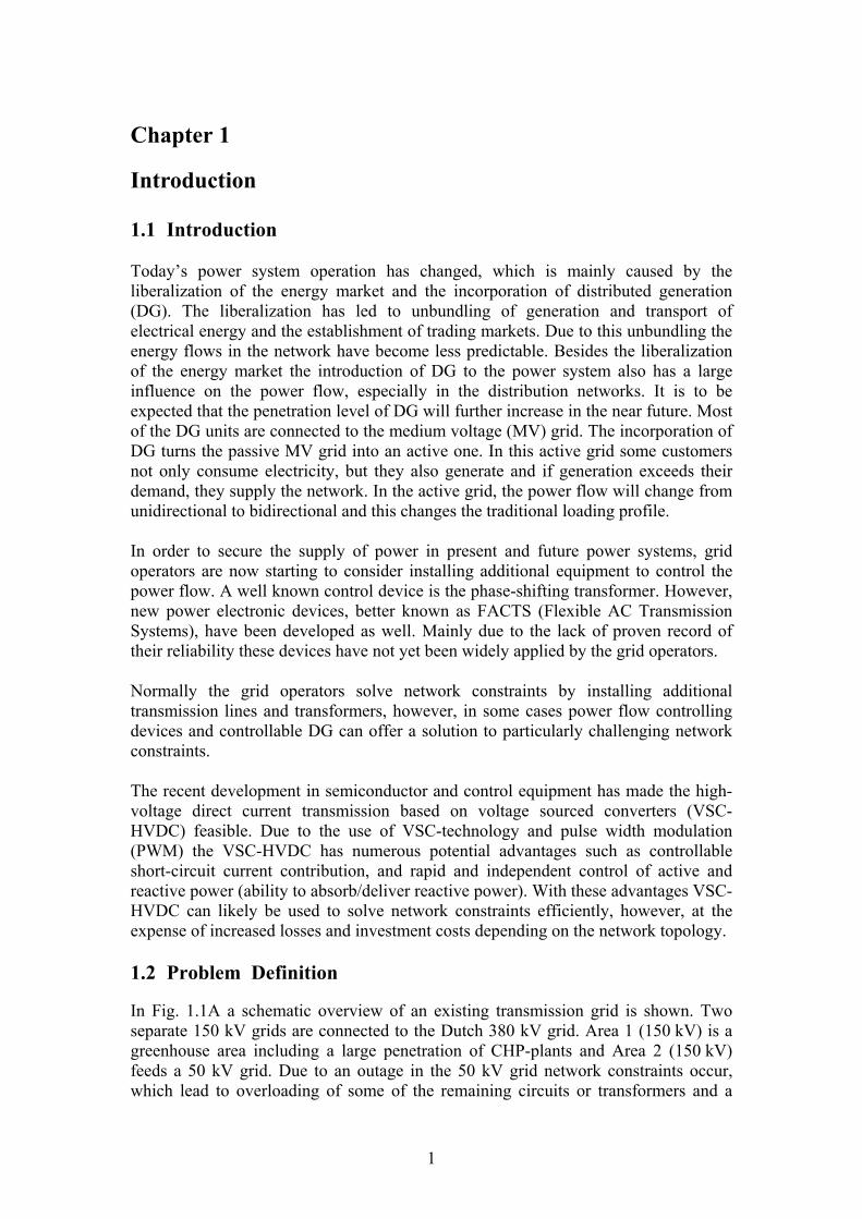
Chapter 1 Introduction 1.1 Introduction Today’s power system operation has changed, which is mainly caused by the liberalization of the energy market and the incorporation of distributed generation (DG). The liberalization has led to unbundling of generation and transport of electrical energy and the establishment of trading markets. Due to this unbundling the energy flows in the network have become less predictable. Besides the liberalization of the energy market the introduction of DG to the power system also has a large influence on the power flow, especially in the distribution networks. It is to be expected that the penetration level of DG will further increase in the near future. Most of the DG units are connected to the medium voltage (MV) grid. The incorporation of DG turns the passive MV grid into an active one. In this active grid some customers not only consume electricity, but they also generate and if generation exceeds their demand, they supply the network. In the active grid, the power flow will change from unidirectional to bidirectional and this changes the traditional loading profile. In order to secure the supply of power in present and future power systems, grid operators are now starting to consider installing additional equipment to control the power flow. A well known control device is the phase-shifting transformer. However, new power electronic devices, better known as FACTS (Flexible AC Transmission Systems), have been developed as well. Mainly due to the lack of proven record of their reliability these devices have not yet been widely applied by the grid operators. Normally the grid operators solve network constraints by installing additional transmission lines and transformers, however, in some cases power flow controlling devices and controllable DG can offer a solution to particularly challenging network constraints. The recent development in semiconductor and control equipment has made the high-voltage direct current transmission based on voltage sourced converters (VSC-HVDC) feasible. Due to the use of VSC-technology and pulse width modulation (PWM) the VSC-HVDC has numerous potential advantages such as controllable short-circuit current contribution, and rapid and independent control of active and reactive power (ability to absorb/deliver reactive power). With these advantages VSC-HVDC can likely be used to solve network constraints efficiently, however, at the expense of increased losses and investment costs depending on the network topology. 1.2 Problem Definition In Fig. 1.1A a schematic overview of an existing transmission grid is shown. Two separate 150 kV grids are connected to the Dutch 380 kV grid. Area 1 (150 kV) is a greenhouse area including a large penetration of CHP-plants and Area 2 (150 kV) feeds a 50 kV grid. Due to an outage in the 50 kV grid network constraints occur, which lead to overloading of some of the remaining circuits or transformers and a
Chapter 1 Introduction
2
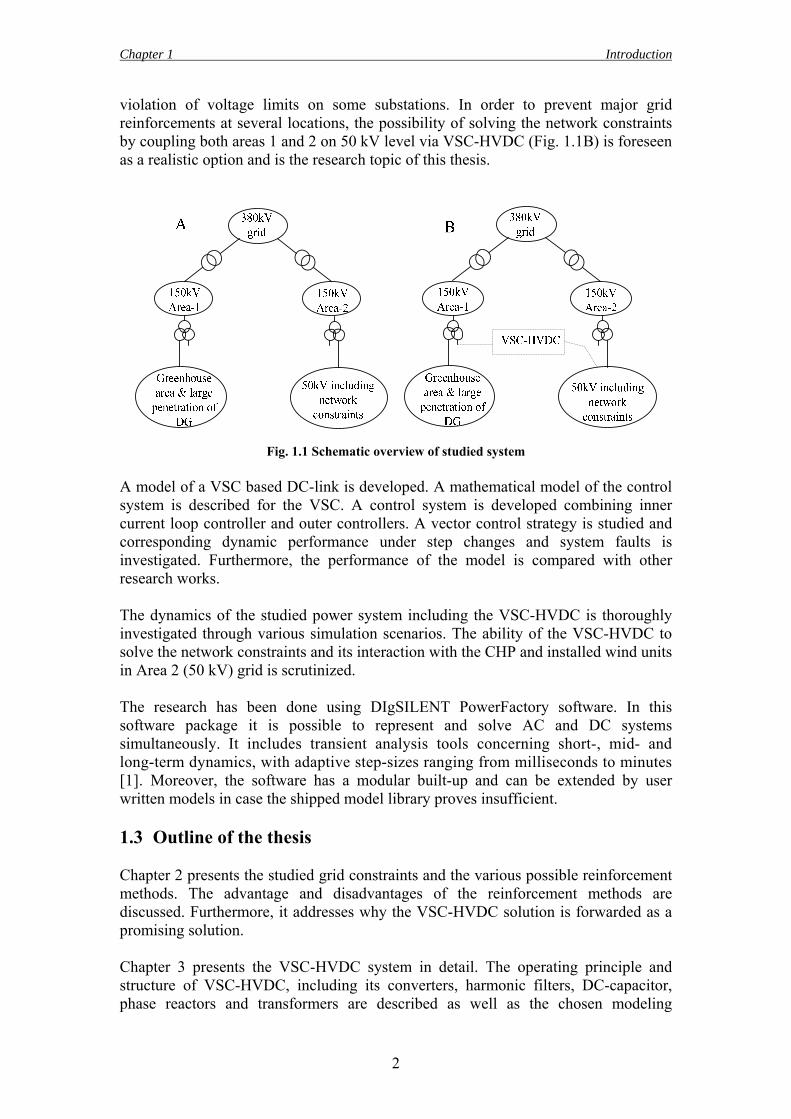
violation of voltage limits on some substations. In order to prevent major grid reinforcements at several locations, the possibility of solving the network constraints by coupling both areas 1 and 2 on 50 kV level via VSC-HVDC (Fig. 1.1B) is foreseen as a realistic option and is the research topic of this thesis.
Fig. 1.1 Schematic overview of studied system
A model of a VSC based DC-link is developed. A mathematical model of the control system is described for the VSC. A control system is developed combining inner current loop controller and outer controllers. A vector control strategy is studied and corresponding dynamic performance under step changes and system faults is investigated. Furthermore, the performance of the model is compared with other research works. The dynamics of the studied power system including the VSC-HVDC is thoroughly investigated through various simulation scenarios. The ability of the VSC-HVDC to solve the network constraints and its interaction with the CHP and installed wind units in Area 2 (50 kV) grid is scrutinized. The research has been done using DIgSILENT PowerFactory software. In this software package it is possible to represent and solve AC and DC systems simultaneously. It includes transient analysis tools concerning short-, mid- and long-term dynamics, with adaptive step-sizes ranging from milliseconds to minutes [1]. Moreover, the software has a modular built-up and can be extended by user written models in case the shipped model library proves insufficient. 1.3 Outline of the thesis Chapter 2 presents the studied grid constraints and the various possible reinforcement methods. The advantage and disadvantages of the reinforcement methods are discussed. Furthermore, it addresses why the VSC-HVDC solution is forwarded as a promising solution. Chapter 3 presents the VSC-HVDC system in detail. The operating principle and structure of VSC-HVDC, including its converters, harmonic filters, DC-capacitor, phase reactors and transformers are described as well as the chosen modeling
Chapter 1 Introduction
3
approach. The design and selection of appropriate parameter values of VSC-HVDC components is given in detail. The mathematical derivation and overall structure of the VSC-HVDC control system is described in chapter 4. Chapter 5 discusses the dynamic performance of the VSC-HVDC under idealized network conditions. In this chapter, step changes in power and voltage, balanced and unbalanced faults are simulated using a test network to evaluate the designed VSC-HVDC control systems. In chapter 6, the VSC-HVDC model is used to couple the two 150 kV Areas on 50 kV level. Various simulation scenarios are investigated to evaluate the performance of the VSC-HVDC as a solution of the network constraints. The interaction of VSC-HVDC with the rest of the grid under various disturbances is also investigated. Finally, the conclusions of the work and some suggestions for future research to deploy the VSC-HVDC in the grid are pointed out in Chapter 7.
4
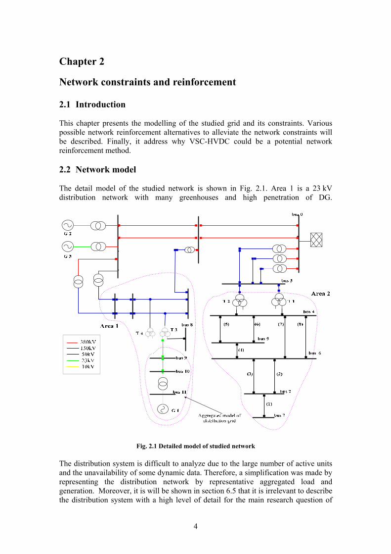
Chapter 2 Network constraints and reinforcement 2.1 Introduction This chapter presents the modelling of the studied grid and its constraints. Various possible network reinforcement alternatives to alleviate the network constraints will be described. Finally, it address why VSC-HVDC could be a potential network reinforcement method. 2.2 Network model The detail model of the studied network is shown in Fig. 2.1. Area 1 is a 23 kV distribution network with many greenhouses and high penetration of DG.
Fig. 2.1 Detailed model of studied network
The distribution system is difficult to analyze due to the large number of active units and the unavailability of some dynamic data. Therefore, a simplification was made by representing the distribution network by representative aggregated load and generation. Moreover, it is will be shown in section 6.5 that it is irrelevant to describe the distribution system with a high level of detail for the main research question of
Chapter 2 Network constraints and reinforcements
5
this thesis. Thus aggregation is used to model the distribution grid; several generators with the same or similar dynamic structures are represented by an equivalent generator model [2, 3]. The equivalent inertia and apparent power are the sum of the inertias and power ratings of all the individual generators. Thus, the distribution grid is modeled as a single synchronous generator rated 50 MVA connected to a step-up transformer of 10/23 kV as shown in Fig. 2.1. Moreover, the equivalent generator model is operated to maintain the same steady state power flow conditions as the detailed model; here it is operated in PQ mode with zero reactive power set point as DG units are operated at unity power factor. The loads are modelled as equivalent constant impedance load (static load) at each substation. The correct modelling of synchronous generators is a very important issue in all kinds of studies of electrical power systems. Here, it is taken the advantage of the highly accurate models [1], which can be used for whole range of different analysis, provided by DIgSILENT software. For both balanced and unbalanced RMS simulations, all the generators G1, G2 and G3 will be of 5th order model, stator transients are ignored and d-q currents remain DC during transients. For EMT simulations, if any, Generator models of 7th order will be used. Generators, G2 and G3 are identical synchronous machines of rated capacity of 625 MVA at 21 kV. Both are fitted with standard excitation system of type IEEET1, governor system of type steam turbine governor (TGOV1) and power system stabilizer (PSS) of type IEEEST which are available in DIgSILENT PowerFactory software as standard library blocks. The block diagrams of these controllers and their parameters are presented in Appendix B. Experimental simulation of a step change in load and terminal voltage, and short-circuits have been made to test the performance of the excitation and governor system by changing the gain parameters. The software default parameters with a slight modification were found to show a reasonably accurate performance. Generator, G1 is fitted with excitation system of type IEEET1 and governor system of type gas turbine generator (pcu_GAST). G1 is not fitted with power system stabilizer (PSS) as actual distribution network active units, small CHP units, do not have a PSS. The same experiment as for G2 and G3 has been made to see the performance of these controllers, DIgSILENT default gain parameters are found to be reasonable. 2.3 Network constraints As a result of the autonomous load growth, several assets in Area 2 will reach their maximum loading capacity in the coming years. Besides, an outage in the 50 kV grid network may cause constraints which lead to overloading of some of the remaining circuits or transformers, and violation of voltage limits. An extensive study of load flow calculation and N-1 contingency analysis taking into account future load growths revealed that the components shown dotted in Fig. 2.2 will be under constraint [4]. Voltage levels within 5%± are assumed to be acceptable.
Chapter 2 Network constraints and reinforcements
6
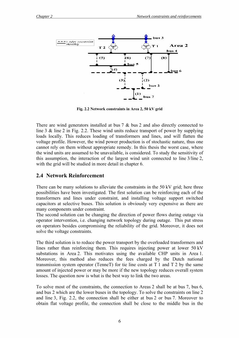
Fig. 2.2 Network constraints in Area 2, 50 kV grid
There are wind generators installed at bus 7 & bus 2 and also directly connected to line 3 & line 2 in Fig. 2.2. These wind units reduce transport of power by supplying loads locally. This reduces loading of transformers and lines, and will flatten the voltage profile. However, the wind power production is of stochastic nature, thus one cannot rely on them without appropriate remedy. In this thesis the worst case, where the wind units are assumed to be unavailable, is considered. To study the sensitivity of this assumption, the interaction of the largest wind unit connected to line 3/line 2, with the grid will be studied in more detail in chapter 6. 2.4 Network Reinforcement There can be many solutions to alleviate the constraints in the 50 kV grid; here three possibilities have been investigated. The first solution can be reinforcing each of the transformers and lines under constraint, and installing voltage support switched capacitors at selective buses. This solution is obviously very expensive as there are many components under constraint. The second solution can be changing the direction of power flows during outage via operator intervention, i.e. changing network topology during outage. This put stress on operators besides compromising the reliability of the grid. Moreover, it does not solve the voltage constraints. The third solution is to reduce the power transport by the overloaded transformers and lines rather than reinforcing them. This requires injecting power at lower 50 kV substations in Area 2. This motivates using the available CHP units in Area 1. Moreover, this method also reduces the fees charged by the Dutch national transmission system operator (TenneT) for tie line costs at T 1 and T 2 by the same amount of injected power or may be more if the new topology reduces overall system losses. The question now is what is the best way to link the two areas. To solve most of the constraints, the connection to Areas 2 shall be at bus 7, bus 6, and bus 2 which are the lower buses in the topology. To solve the constraints on line 2 and line 3, Fig. 2.2, the connection shall be either at bus 2 or bus 7. Moreover to obtain flat voltage profile, the connection shall be close to the middle bus in the
Chapter 2 Network constraints and reinforcements
7
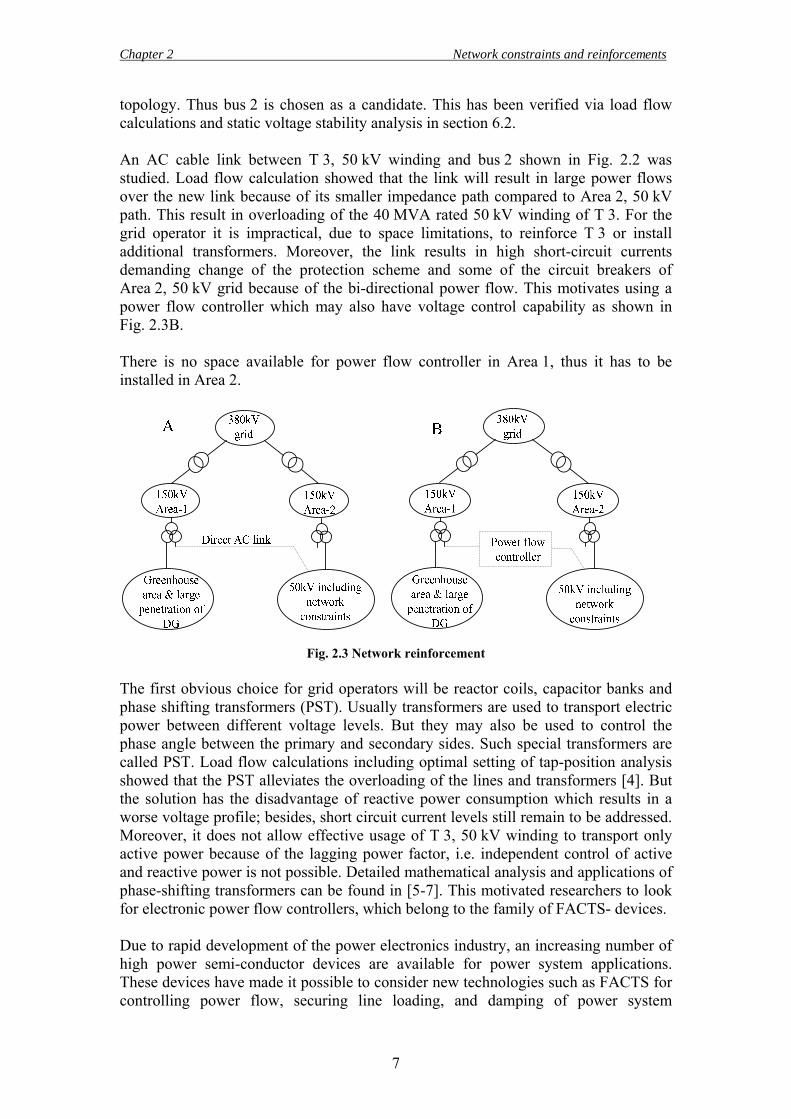
topology. Thus bus 2 is chosen as a candidate. This has been verified via load flow calculations and static voltage stability analysis in section 6.2. An AC cable link between T 3, 50 kV winding and bus 2 shown in Fig. 2.2 was studied. Load flow calculation showed that the link will result in large power flows over the new link because of its smaller impedance path compared to Area 2, 50 kV path. This result in overloading of the 40 MVA rated 50 kV winding of T 3. For the grid operator it is impractical, due to space limitations, to reinforce T 3 or install additional transformers. Moreover, the link results in high short-circuit currents demanding change of the protection scheme and some of the circuit breakers of Area 2, 50 kV grid because of the bi-directional power flow. This motivates using a power flow controller which may also have voltage control capability as shown in Fig. 2.3B. There is no space available for power flow controller in Area 1, thus it has to be installed in Area 2.
Fig. 2.3 Network reinforcement
The first obvious choice for grid operators will be reactor coils, capacitor banks and phase shifting transformers (PST). Usually transformers are used to transport electric power between different voltage levels. But they may also be used to control the phase angle between the primary and secondary sides. Such special transformers are called PST. Load flow calculations including optimal setting of tap-position analysis showed that the PST alleviates the overloading of the lines and transformers [4]. But the solution has the disadvantage of reactive power consumption which results in a worse voltage profile; besides, short circuit current levels still remain to be addressed. Moreover, it does not allow effective usage of T 3, 50 kV winding to transport only active power because of the lagging power factor, i.e. independent control of active and reactive power is not possible. Detailed mathematical analysis and applications of phase-shifting transformers can be found in [5-7]. This motivated researchers to look for electronic power flow controllers, which belong to the family of FACTS- devices. Due to rapid development of the power electronics industry, an increasing number of high power semi-conductor devices are available for power system applications. These devices have made it possible to consider new technologies such as FACTS for controlling power flow, securing line loading, and damping of power system
Chapter 2 Network constraints and reinforcements
8
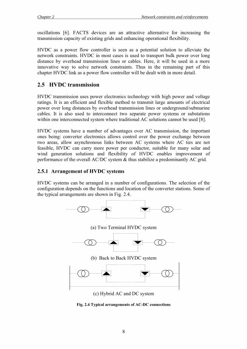
oscillations [6]. FACTS devices are an attractive alternative for increasing the transmission capacity of existing grids and enhancing operational flexibility. HVDC as a power flow controller is seen as a potential solution to alleviate the network constraints. HVDC in most cases is used to transport bulk power over long distance by overhead transmission lines or cables. Here, it will be used in a more innovative way to solve network constraints. Thus in the remaining part of this chapter HVDC link as a power flow controller will be dealt with in more detail. 2.5 HVDC transmission HVDC transmission uses power electronics technology with high power and voltage ratings. It is an efficient and flexible method to transmit large amounts of electrical power over long distances by overhead transmission lines or underground/submarine cables. It is also used to interconnect two separate power systems or substations within one interconnected system where traditional AC solutions cannot be used [8]. HVDC systems have a number of advantages over AC transmission, the important ones being: converter electronics allows control over the power exchange between two areas, allow asynchronous links between AC systems where AC ties are not feasible, HVDC can carry more power per conductor, suitable for many solar and wind generation solutions and flexibility of HVDC enables improvement of performance of the overall AC/DC system & thus stabilize a predominantly AC grid. 2.5.1 Arrangement of HVDC systems HVDC systems can be arranged in a number of configurations. The selection of the configuration depends on the functions and location of the converter stations. Some of the typical arrangements are shown in Fig. 2.4.
(a) Two Terminal HVDC system
(b) Back to Back HVDC system
(c) Hybrid AC and DC system
Fig. 2.4 Typical arrangements of AC-DC connections
Chapter 2 Network constraints and reinforcements
9
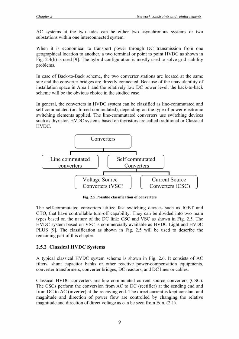
AC systems at the two sides can be either two asynchronous systems or two substations within one interconnected system. When it is economical to transport power through DC transmission from one geographical location to another, a two terminal or point to point HVDC as shown in Fig. 2.4(b) is used [9]. The hybrid configuration is mostly used to solve grid stability problems. In case of Back-to-Back scheme, the two converter stations are located at the same site and the converter bridges are directly connected. Because of the unavailability of installation space in Area 1 and the relatively low DC power level, the back-to-back scheme will be the obvious choice in the studied case. In general, the converters in HVDC system can be classified as line-commutated and self-commutated (or: forced commutated), depending on the type of power electronic switching elements applied. The line-commutated converters use switching devices such as thyristor. HVDC systems based on thyristors are called traditional or Classical HVDC.
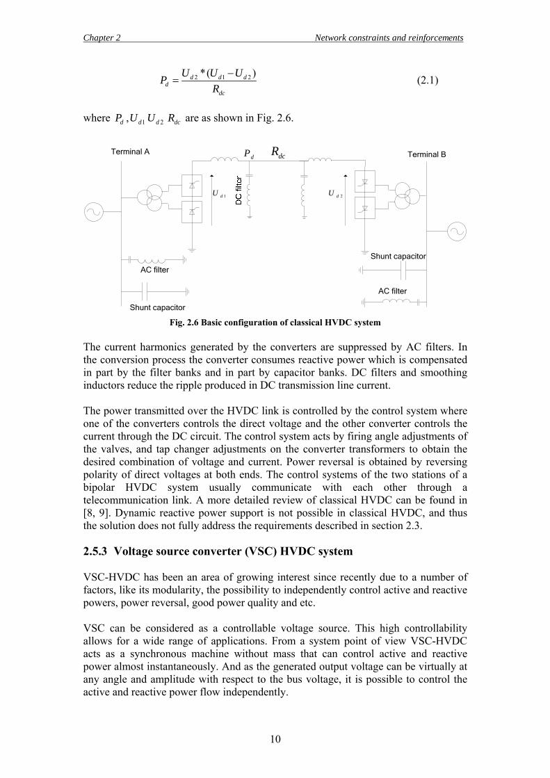
Fig. 2.5 Possible classification of converters The self-commutated converters utilize fast switching devices such as IGBT and GTO, that have controllable turn-off capability. They can be divided into two main types based on the nature of the DC link: CSC and VSC as shown in Fig. 2.5. The HVDC system based on VSC is commercially available as HVDC Light and HVDC PLUS [9]. The classification as shown in Fig. 2.5 will be used to describe the remaining part of this chapter. 2.5.2 Classical HVDC Systems A typical classical HVDC system scheme is shown in Fig. 2.6. It consists of AC filters, shunt capacitor banks or other reactive power-compensation equipments, converter transformers, converter bridges, DC reactors, and DC lines or cables. Classical HVDC converters are line commutated current source converters (CSC). The CSCs perform the conversion from AC to DC (rectifier) at the sending end and from DC to AC (inverter) at the receiving end. The direct current is kept constant and magnitude and direction of power flow are controlled by changing the relative magnitude and direction of direct voltage as can be seen from Eqn. (2.1).
Converters
Line commutated converters
Self commutated Converters
Voltage Source Converters (VSC)
Current Source Converters (CSC)
Chapter 2 Network constraints and reinforcements
10
2 1 2*( )d d dd
dc
U U UPR
−= (2.1)
where dP , 1dU 2dU dcR are as shown in Fig. 2.6.
AC filter
Shunt capacitor
Terminal BTerminal A
AC filter
Shunt capacitor
dcR
1dU 2dU
dP
Fig. 2.6 Basic configuration of classical HVDC system
The current harmonics generated by the converters are suppressed by AC filters. In the conversion process the converter consumes reactive power which is compensated in part by the filter banks and in part by capacitor banks. DC filters and smoothing inductors reduce the ripple produced in DC transmission line current. The power transmitted over the HVDC link is controlled by the control system where one of the converters controls the direct voltage and the other converter controls the current through the DC circuit. The control system acts by firing angle adjustments of the valves, and tap changer adjustments on the converter transformers to obtain the desired combination of voltage and current. Power reversal is obtained by reversing polarity of direct voltages at both ends. The control systems of the two stations of a bipolar HVDC system usually communicate with each other through a telecommunication link. A more detailed review of classical HVDC can be found in [8, 9]. Dynamic reactive power support is not possible in classical HVDC, and thus the solution does not fully address the requirements described in section 2.3. 2.5.3 Voltage source converter (VSC) HVDC system VSC-HVDC has been an area of growing interest since recently due to a number of factors, like its modularity, the possibility to independently control active and reactive powers, power reversal, good power quality and etc. VSC can be considered as a controllable voltage source. This high controllability allows for a wide range of applications. From a system point of view VSC-HVDC acts as a synchronous machine without mass that can control active and reactive power almost instantaneously. And as the generated output voltage can be virtually at any angle and amplitude with respect to the bus voltage, it is possible to control the active and reactive power flow independently.
Chapter 2 Network constraints and reinforcements
11
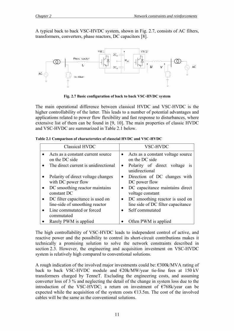
A typical back to back VSC-HVDC system, shown in Fig. 2.7, consists of AC filters, transformers, converters, phase reactors, DC capacitors [8].
2 dcC
2 dcC
dcu
u v
Fig. 2.7 Basic configuration of back to back VSC-HVDC system
The main operational difference between classical HVDC and VSC-HVDC is the higher controllability of the latter. This leads to a number of potential advantages and applications related to power flow flexibility and fast response to disturbances, where extensive list of them can be found in [9, 10]. The main properties of classic HVDC and VSC-HVDC are summarized in Table 2.1 below. Table 2.1 Comparison of characterstics of classcial HVDC and VSC-HVDC
Classical HVDC VSC-HVDC • Acts as a constant current source
on the DC side • The direct current is unidirectional • Polarity of direct voltage changes
with DC power flow • DC smoothing reactor maintains
constant DC • DC filter capacitance is used on
line-side of smoothing reactor • Line commutated or forced
commutated • Rarely PWM is applied
• Acts as a constant voltage source on the DC side
• Polarity of direct voltage is unidirectional
• Direction of DC changes with DC power flow
• DC capacitance maintains direct voltage constant
• DC smoothing reactor is used on line side of DC filter capacitance
• Self commutated • Often PWM is applied
The high controllability of VSC-HVDC leads to independent control of active, and reactive power and the possibility to control its short-circuit contributions makes it technically a promising solution to solve the network constraints described in section 2.3. However, the engineering and acquisition investment on VSC-HVDC system is relatively high compared to conventional solutions. A rough indication of the involved major investments could be: €300k/MVA rating of back to back VSC-HVDC module and €20k/MW/year tie-line fees at 150 kV transformers charged by TenneT. Excluding the engineering costs, and assuming converter loss of 3 % and neglecting the detail of the change in system loss due to the introduction of the VSC-HVDC; a return on investment of €768k/year can be expected while the acquisition of the system costs €13.5m. The cost of the involved cables will be the same as the conventional solutions.
Chapter 2 Network constraints and reinforcements
12
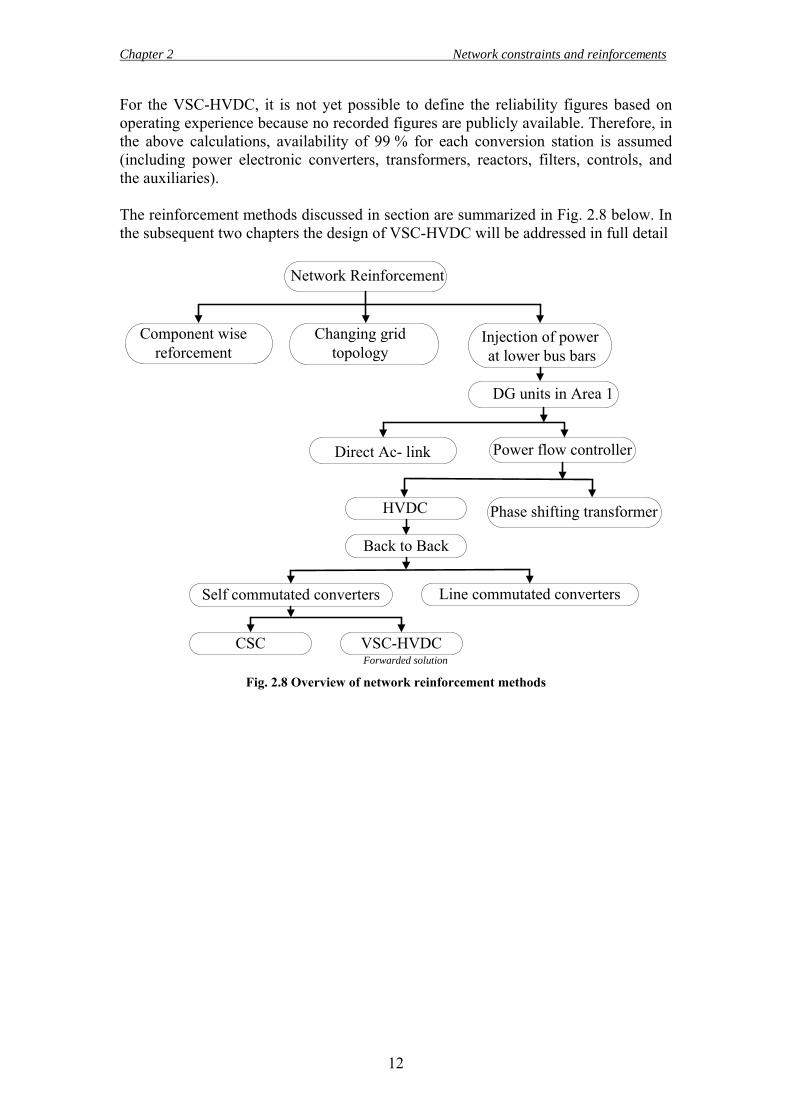
For the VSC-HVDC, it is not yet possible to define the reliability figures based on operating experience because no recorded figures are publicly available. Therefore, in the above calculations, availability of 99 % for each conversion station is assumed (including power electronic converters, transformers, reactors, filters, controls, and the auxiliaries). The reinforcement methods discussed in section are summarized in Fig. 2.8 below. In the subsequent two chapters the design of VSC-HVDC will be addressed in full detail
Network Reinforcement
Injection of powerat lower bus bars
Changing grid topology
Component wise reforcement
Forwarded solution
DG units in Area 1
Direct Ac- link Power flow controller
Phase shifting transformer HVDC
Back to Back
Self commutated converters Line commutated converters
CSC VSC-HVDC
Fig. 2.8 Overview of network reinforcement methods
13
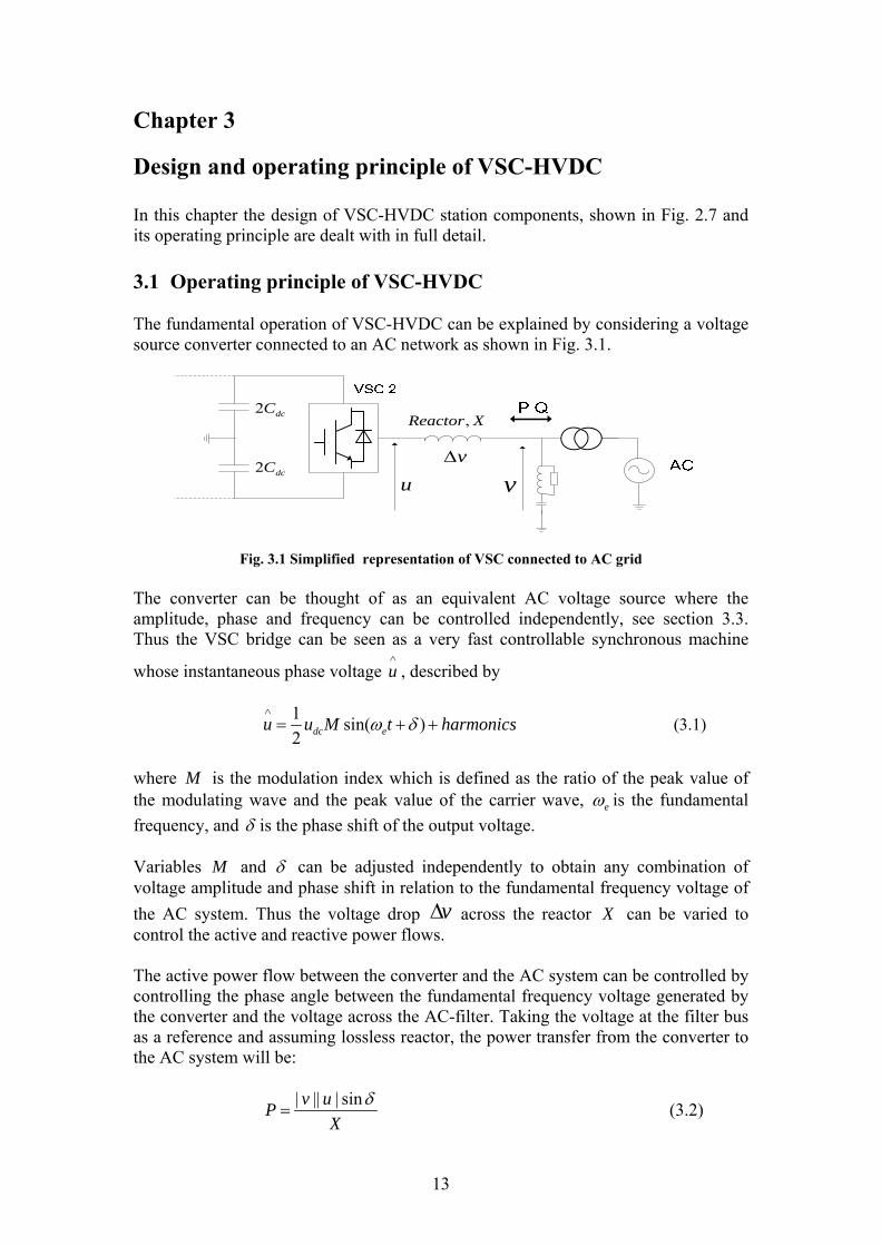
Chapter 3 Design and operating principle of VSC-HVDC In this chapter the design of VSC-HVDC station components, shown in Fig. 2.7 and its operating principle are dealt with in full detail. 3.1 Operating principle of VSC-HVDC The fundamental operation of VSC-HVDC can be explained by considering a voltage source converter connected to an AC network as shown in Fig. 3.1.
,Reactor X
u vvΔ
2 dcC
2 dcC
Fig. 3.1 Simplified representation of VSC connected to AC grid The converter can be thought of as an equivalent AC voltage source where the amplitude, phase and frequency can be controlled independently, see section 3.3. Thus the VSC bridge can be seen as a very fast controllable synchronous machine
whose instantaneous phase voltage u∧
, described by
1 sin( )2 dc eu u M t harmonicsω δ
∧
= + + (3.1)
where M is the modulation index which is defined as the ratio of the peak value of the modulating wave and the peak value of the carrier wave, eω is the fundamental frequency, and δ is the phase shift of the output voltage. Variables M and δ can be adjusted independently to obtain any combination of voltage amplitude and phase shift in relation to the fundamental frequency voltage of the AC system. Thus the voltage drop vΔ across the reactor X can be varied to control the active and reactive power flows. The active power flow between the converter and the AC system can be controlled by controlling the phase angle between the fundamental frequency voltage generated by the converter and the voltage across the AC-filter. Taking the voltage at the filter bus as a reference and assuming lossless reactor, the power transfer from the converter to the AC system will be:
| || | sinv uPX
δ= (3.2)

Chapter 3 Design and operating principle of VSC-HVDC
14
The reactive power flow is determined by the relative difference in magnitude between the converter and filter voltages. The reactive power flow is calculated as:
| | (| | | | cos )v v uQX
δ−= (3.3)
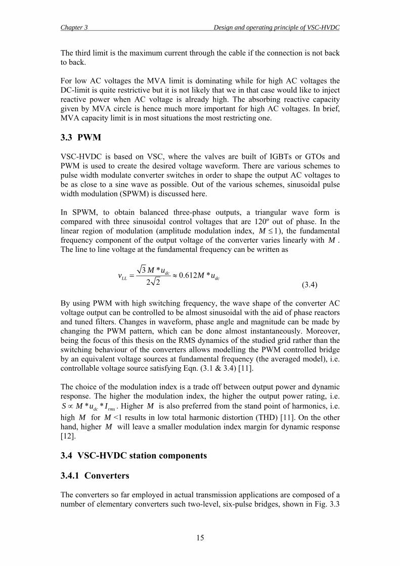
The active power flow on the AC side is equal to the active power transmitted from the DC side in steady state, disregarding the losses. This can be fulfilled if one of the two converters controls the active power transmitted and the other controls the direct voltage. The reactive power generated/consumed by the converter is adjusted to control AC network voltage or/and reactive power injections. 3.2 Capability chart of VSC -HVDC It is common to describe the capability of a power apparatus in a number of different ways, i.e. showing under what conditions it can operate. Active power and reactive power capability is usually illustrated in the P–Q plane. There are mainly three factors that limit the active and reactive power output of VSC-HVDC as shown in Fig. 3.2. The first limiting factor is the maximum current through the IGBT valves. This leads to the maximum MVA circle in the MVA plane where the maximum current and the actual AC voltage are multiplied. If the AC voltage decreases, so will the MVA capability be reduced proportionally to the voltage drop.
| | 1u =
| | 0.9u =
| | 1.1u =
Fig. 3.2 Capability curve of VSC-HVDC
The second limiting factor is the maximum direct voltage. The AC-voltage generated by the converter is limited by the allowable maximum direct voltage. The reactive power is mainly dependent on the voltage difference between the AC voltage the VSC can generate from the direct voltage and the AC grid voltage. If the grid AC voltage is high the difference between the AC voltage generated by the converter and the grid AC voltage will be low. The reactive power capability is then moderate but increases with decreasing AC voltage. This makes sense from a stability point of view.
Chapter 3 Design and operating principle of VSC-HVDC
15
The third limit is the maximum current through the cable if the connection is not back to back. For low AC voltages the MVA limit is dominating while for high AC voltages the DC-limit is quite restrictive but it is not likely that we in that case would like to inject reactive power when AC voltage is already high. The absorbing reactive capacity given by MVA circle is hence much more important for high AC voltages. In brief, MVA capacity limit is in most situations the most restricting one. 3.3 PWM VSC-HVDC is based on VSC, where the valves are built of IGBTs or GTOs and PWM is used to create the desired voltage waveform. There are various schemes to pulse width modulate converter switches in order to shape the output AC voltages to be as close to a sine wave as possible. Out of the various schemes, sinusoidal pulse width modulation (SPWM) is discussed here. In SPWM, to obtain balanced three-phase outputs, a triangular wave form is compared with three sinusoidal control voltages that are 120º out of phase. In the linear region of modulation (amplitude modulation index, 1M ≤ ), the fundamental frequency component of the output voltage of the converter varies linearly with M . The line to line voltage at the fundamental frequency can be written as
3 * 0.612 *2 2
dcLL dc
M uv M u= ≈ (3.4)
By using PWM with high switching frequency, the wave shape of the converter AC voltage output can be controlled to be almost sinusoidal with the aid of phase reactors and tuned filters. Changes in waveform, phase angle and magnitude can be made by changing the PWM pattern, which can be done almost instantaneously. Moreover, being the focus of this thesis on the RMS dynamics of the studied grid rather than the switching behaviour of the converters allows modelling the PWM controlled bridge by an equivalent voltage sources at fundamental frequency (the averaged model), i.e. controllable voltage source satisfying Eqn. (3.1 & 3.4) [11]. The choice of the modulation index is a trade off between output power and dynamic response. The higher the modulation index, the higher the output power rating, i.e.
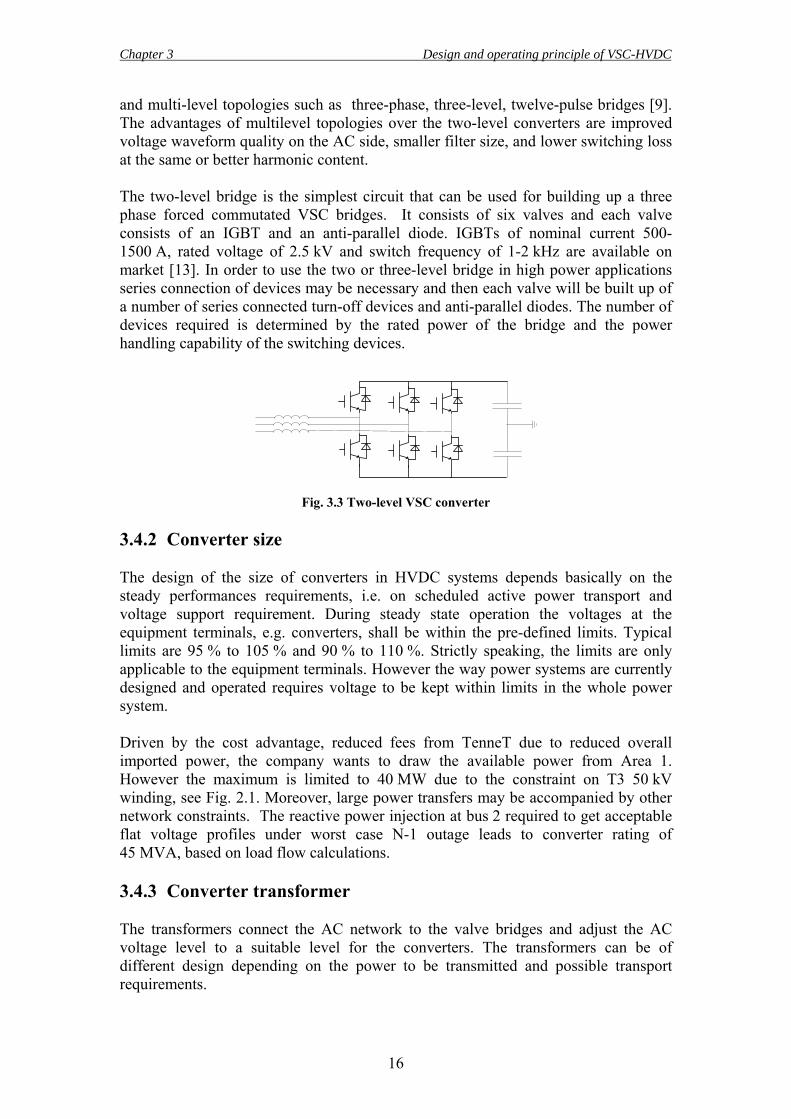
* *dc rmsS M u I∝ . Higher M is also preferred from the stand point of harmonics, i.e. high M for M <1 results in low total harmonic distortion (THD) [11]. On the other hand, higher M will leave a smaller modulation index margin for dynamic response [12]. 3.4 VSC-HVDC station components 3.4.1 Converters The converters so far employed in actual transmission applications are composed of a number of elementary converters such two-level, six-pulse bridges, shown in Fig. 3.3
Chapter 3 Design and operating principle of VSC-HVDC
16
and multi-level topologies such as three-phase, three-level, twelve-pulse bridges [9]. The advantages of multilevel topologies over the two-level converters are improved voltage waveform quality on the AC side, smaller filter size, and lower switching loss at the same or better harmonic content. The two-level bridge is the simplest circuit that can be used for building up a three phase forced commutated VSC bridges. It consists of six valves and each valve consists of an IGBT and an anti-parallel diode. IGBTs of nominal current 500-1500 A, rated voltage of 2.5 kV and switch frequency of 1-2 kHz are available on market [13]. In order to use the two or three-level bridge in high power applications series connection of devices may be necessary and then each valve will be built up of a number of series connected turn-off devices and anti-parallel diodes. The number of devices required is determined by the rated power of the bridge and the power handling capability of the switching devices.
Fig. 3.3 Two-level VSC converter 3.4.2 Converter size The design of the size of converters in HVDC systems depends basically on the steady performances requirements, i.e. on scheduled active power transport and voltage support requirement. During steady state operation the voltages at the equipment terminals, e.g. converters, shall be within the pre-defined limits. Typical limits are 95 % to 105 % and 90 % to 110 %. Strictly speaking, the limits are only applicable to the equipment terminals. However the way power systems are currently designed and operated requires voltage to be kept within limits in the whole power system. Driven by the cost advantage, reduced fees from TenneT due to reduced overall imported power, the company wants to draw the available power from Area 1. However the maximum is limited to 40 MW due to the constraint on T3 50 kV winding, see Fig. 2.1. Moreover, large power transfers may be accompanied by other network constraints. The reactive power injection at bus 2 required to get acceptable flat voltage profiles under worst case N-1 outage leads to converter rating of 45 MVA, based on load flow calculations. 3.4.3 Converter transformer The transformers connect the AC network to the valve bridges and adjust the AC voltage level to a suitable level for the converters. The transformers can be of different design depending on the power to be transmitted and possible transport requirements.
Chapter 3 Design and operating principle of VSC-HVDC
17
Using IGBT valves of nominal current of 500 A, transmitted DC power of 40 MW, AC-side grid voltage of 50 kV, and steady state modulation index of 0.85M = for reasons described in section 3.3, and Eqn. (3.4) and dc dc dcP I u= , the turn ratio of the transformer will be 1.12. Thus it is decided not to include the transformer in the VSC-HVDC model. In fact converter transformer has other advantage besides just merely transforming the voltage levels. It has tap changers which can help in regulating the voltage. But within the time frame of interest of this thesis, the tap-changers are not expected to react. Thus the absence of the converter transformers does not deteriorate the accuracy of our VSC- HVDC model, though the ability of managing zero-sequence currents will be lost. This will be addressed in detail in chapter 5. Moreover, the transfer of active power is still possible due to the presence of phase reactors, section 3.4.6. 3.4.4 Direct voltage The large proportion of the cost of HVDC links is the cost of the converter bridges. Thus the choice of the voltage levels mainly depends on economical issues. Higher voltage levels require many valves to be put in series, thus higher costs. Technically, the minimum direct-voltage level required to avoid converter saturation while using sinusoidal Pulse width modulation can be calculated from Eqn. (3.4) with
1M = , and is given by Eqn. (3.5).
minmin 0.612
LLdc
vu = (3.5)
The maximum direct voltage depends on the design steady state modulation index. In most commercial applications 0.9M < [13] is taken as a design parameter. The maximum direct voltage level is given by Eqn. (3.6).
maxmax 0.612*
LLdc
vuM
= (3.6)
where maxLLv and minLLv are the maximum and minimum steady state acceptable AC-voltage level, 105 % and 95 %, respectively. With a steady state modulation index of 0.85M = , a direct voltage of 100 kV which is within the above two limits is chosen as a design value. 3.4.5 DC capacitor In steady state assuming no losses in the DC link, the instantaneous power on the DC side must equal the instantaneous power on the AC side. In the moment the power balance is broken, the instantaneous difference in power is stored in the DC link capacitor and this leads to fluctuations in the direct voltage. Thus instantaneous current flows in the DC link given by
Chapter 3 Design and operating principle of VSC-HVDC
18
dcc dc
dui Cdt
= (3.7)
Due to PWM switching action in VSC-HVDC, the DC link capacitor current contains harmonics, which will result in a ripple on the DC side voltage. This ripple must be small enough for the voltage to be virtually constant during switching period. This sets a lower limit on the capacitor size. Small voltage ripples require large capacitor, which on the one side has a slow response to voltage changes, but on the other side has a smaller current and thus increased lifetime. On the other hand, a small capacitor makes fast changes in the direct voltage possible allowing fast control of active power at the expense of higher voltage ripples and reduced lifetime. Selecting the size of the DC capacitor has thus to be a trade-off between voltage ripples, lifetime and the fast control of the DC link. The trade off relation for the design of the DC-link capacitor in the back-back converter is described in [9, 14] as follows
* *2*
Ndc
dcN dc e
SCu u ω
=Δ
(3.8)
20.5 dc dcN
N
C uS
τ = (3.9)
where dcNu denotes the nominal direct voltage and NS stands for the nominal apparent power of the converter. The time constant τ is equal to the time needed to charge the capacitor from zero to rated voltage dcNu when the converter is supplied with a constant active power equal to NS . dcuΔ denotes the allowed ripple (peak to peak), and eω the electrical frequency. Eqn. (3.8 & 3.9) sets the lower and upper limits of the size of DC-capacitor respectively. The time constant τ is selected to be less than 10 ms to satisfy small ripple and transient overvoltage on the DC-link. A capacitance of 37.5 µF which result in a peak to peak percentage ripple of 18 % is used. 3.4.6 Phase reactor The phase reactors, as shown in Fig. 2.7, are used for controlling both the active and the reactive power flow by regulating currents through them. The reactors also functions as AC filters to reduce the high frequency harmonic content of the AC currents which are caused by the switching operation of the VSCs. The reactors are essential for both the active and reactive power flow, since these properties are determined by the power frequency voltage across the reactors. The choice of the size of the phase reactor depends on the switching frequency, converter saturation and control algorithm, converter saturation being the dominant determinant factor. In vector controlled-VSC-HVDC, section 4.3, the phase reactor L is chosen such that the minimum reference current tracking time tΔ is less than the

Chapter 3 Design and operating principle of VSC-HVDC
19
time constant of the converter current controller [15] , governed by Eqn. (3.10). Thus converter saturation and control put the upper threshold while current smoothing, active power and reactive power controls may put lower threshold for the phase reactor. The phase reactors are usually in the range of 0.1 pu to 0.2 pu [9, 13, 14].
max
0.9 0.612*( ) dc
e LL LL
Lt uv vω
Δ =−
(3.10)
where LLv (pu) denotes the AC- side voltage, L (pu)-smoothing reactor inductance and
maxLLv (pu) stands for the theoretical maximum amplitude of the converter fundamental phase voltage, i.e. 0.612 dcu for sinusoidal PWM, see Eqn. (3.4). It should be noted that this value changes with the specific type of PWM used. 3.4.7 AC filters The AC voltage output contains the fundamental AC component plus higher-order harmonic, derived from the switching of the IGBT’s. These harmonics have to be taken care of preventing them from being emitted into the AC system so that sinusoidal line currents and voltages can be obtained at the point of common coupling (PCC). High pass filters are installed to take care of these high order harmonics. Moreover they serve as source of reactive power. As stated in [11], a PWM output waveform contains harmonics 1cKf Nf± where cf is the carrier frequency, 1f is the fundamental grid frequency. K and N are integers and their sum is an odd integer. Next to the fundamental frequency component, the spectrum of the output voltages contains components around the carrier frequency of the PWM and multiples of the carrier frequency. With the use of PWM, passive high-pass damped filters are selected to filter the high order harmonics. Normally, a second order high-pass filter (see Fig. 3.4), the characteristic frequency of which is selected based on the switching [9], is used in VSC-HVDC systems. In RMS type simulations the filter solely injects reactive power at fundamental frequency and does not need to be represented in full detail.
filterR
filterC
filterL
Fig. 3.4 passive second order high pass filter
Quality factor fQ of typical values between 0.5 % and 5 % [9], AC-filter rating,
filterQ and harmonic order h are used as a design parameters. The resistance filterR ,
Chapter 3 Design and operating principle of VSC-HVDC
20
capacitance filterC and inductances filterL are calculated based on the following equations
2
2 2
( 1) filterfilter
e LL
h QC
h vω−
= (3.11)
2 2
1filter
filter e
LC h ω
= (3.12)
filterfilter f
filter
LR Q
C= (3.13)
In this thesis typical values of filterQ =15 % of converter rating [13], fQ =3 % [9, 13], and h=35 are used as design inputs. Remark should be taken that these values depends on harmonic requirements of the specific system under study.
21
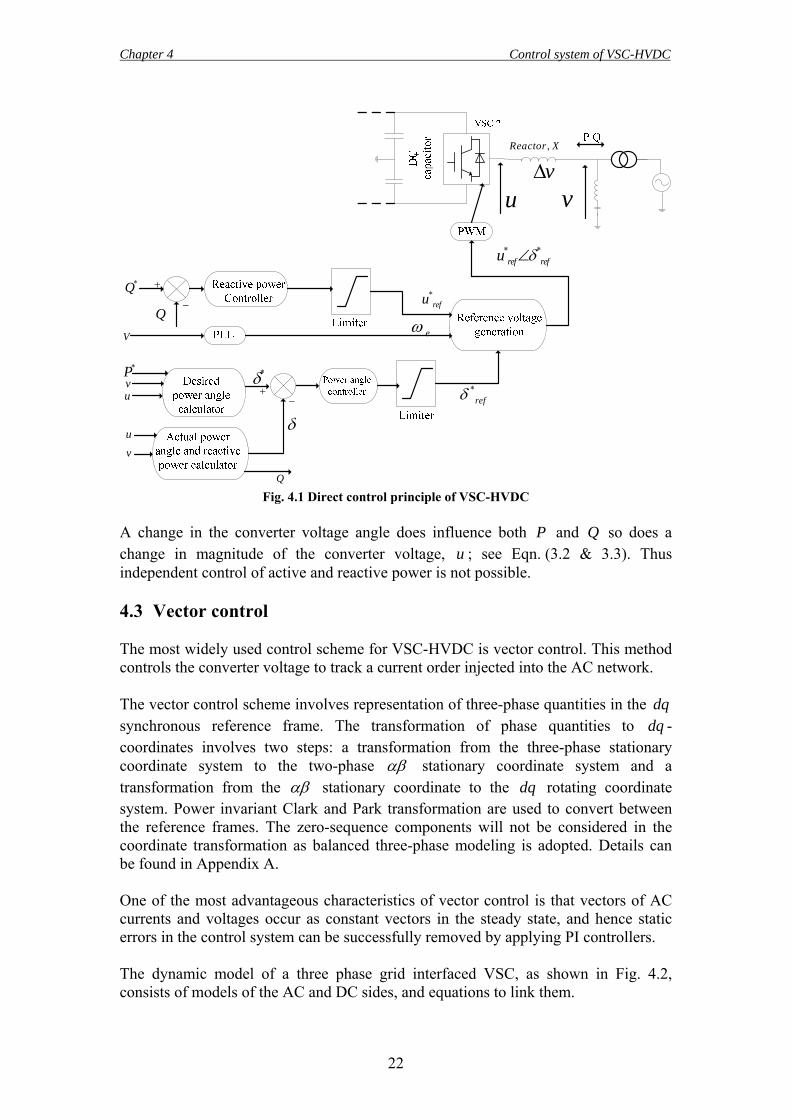
Chapter 4 Control system of VSC-HVDC 4.1 Introduction The control of a VSC-HVDC system is basically the control of the transfer of energy. The aim of the control in VSC based HVDC transmission is thus the accurate control of transmitted active and reactive power. Moreover, the VSC controls are often used to provide ancillary services, such as improve the dynamics of AC grids. Different control strategies are found in literature for the control of VSC-HVDC. Direct control and vector control methods which are based on voltage controlled VSC and current controlled VSC schemes respectively are the most widely used methods. In voltage-controlled schemes, the active and reactive power is controlled directly by controlling the phase angle and amplitude of the converter output voltage. On the other hand, the current controlled scheme utilizes the converters as a controllable current source, where the injected current vector follows a reference current vector. The current-controlled VSC offers potential advantages over the voltage-controlled VSC. The mains advantages being: 1) better power quality as the current-controller converter is less affected by grid harmonics and disturbances, 2) decoupled control of active and reactive power, 3) inherent protection against over currents, and 4) the control mode can be easily extended to compensate for line harmonics and other power quality issues [16]. The vector control method is widely used in VSC-HVDC and will also be adopted in this thesis. 4.2 Direct control The direct control method uses voltage control of the VSC. The active and reactive power flows are controlled by directly altering the phase shift δ , and the modulation index M thus the magnitude of the converter voltage, see Eqns. (3.2 & 3.3). The actual power angle is calculated from the terminal quantities and compared to the desired power angle, which is calculated from the active power order. The error in the power angle is processed by a power angle controller to generate the reference phase angle of the modulating signal. In a similar manner, the error between the actual and desired reactive power is processed by a reactive power controller to generate the magnitude reference of the modulating signal. A phase-locked loop (PLL) circuit is responsible for synchronizing the converter output voltage with the AC grid. The control scheme is shown in Fig. 4.1.
Chapter 4 Control system of VSC-HVDC
22
,Reactor X
u vvΔ
Q
*Q
Q
uv
*P *δ
δ
*refδ
*refu
* *ref refu δ∠
eω
uv
−
−
+
+
V
Fig. 4.1 Direct control principle of VSC-HVDC
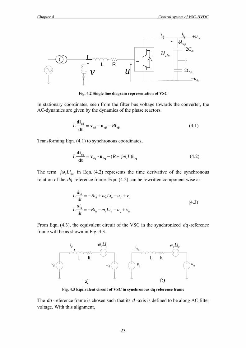
A change in the converter voltage angle does influence both P and Q so does a change in magnitude of the converter voltage, u ; see Eqn. (3.2 & 3.3). Thus independent control of active and reactive power is not possible. 4.3 Vector control The most widely used control scheme for VSC-HVDC is vector control. This method controls the converter voltage to track a current order injected into the AC network. The vector control scheme involves representation of three-phase quantities in the dq synchronous reference frame. The transformation of phase quantities to dq -coordinates involves two steps: a transformation from the three-phase stationary coordinate system to the two-phase αβ stationary coordinate system and a transformation from the αβ stationary coordinate to the dq rotating coordinate system. Power invariant Clark and Park transformation are used to convert between the reference frames. The zero-sequence components will not be considered in the coordinate transformation as balanced three-phase modeling is adopted. Details can be found in Appendix A. One of the most advantageous characteristics of vector control is that vectors of AC currents and voltages occur as constant vectors in the steady state, and hence static errors in the control system can be successfully removed by applying PI controllers. The dynamic model of a three phase grid interfaced VSC, as shown in Fig. 4.2, consists of models of the AC and DC sides, and equations to link them.
Chapter 4 Control system of VSC-HVDC
23
i
v uL R
dcucapi
dci Lidcu+
dcu−2 dcC
2 dcC
Fig. 4.2 Single line diagram representation of VSC In stationary coordinates, seen from the filter bus voltage towards the converter, the AC-dynamics are given by the dynamics of the phase reactors.
L R= − −αβαβ αβ αβ
div u i
dt (4.1)
Transforming Eqn. (4.1) to synchronous coordinates,
( )eL R j Lω= − +dqdq dq dq
div - u i
dt (4.2)
The term e dqj Liω in Eqn. (4.2) represents the time derivative of the synchronous rotation of the dq reference frame. Eqn. (4.2) can be rewritten component wise as
dd e q d d
qq e d q q
diL Ri Li u vdtdi
L Ri Li u vdt
ω
ω
= − + − +
= − − − + (4.3)
From Eqn. (4.3), the equivalent circuit of the VSC in the synchronized dq -reference frame will be as shown in Fig. 4.3.
e qLiωdi
dudv
e dLiωqi
quqv
Fig. 4.3 Equivalent circuit of VSC in synchronous dq reference frame
The dq -reference frame is chosen such that its d -axis is defined to be along AC filter voltage. With this alignment,
Chapter 4 Control system of VSC-HVDC
24
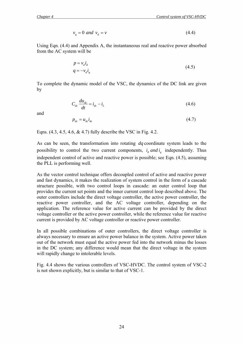
0q dv and v v= = (4.4) Using Eqn. (4.4) and Appendix A, the instantaneous real and reactive power absorbed from the AC system will be
d d
d q
p v iq v i== −
(4.5)
To complete the dynamic model of the VSC, the dynamics of the DC link are given by
dcdc dc L
duC i idt
= − (4.6)
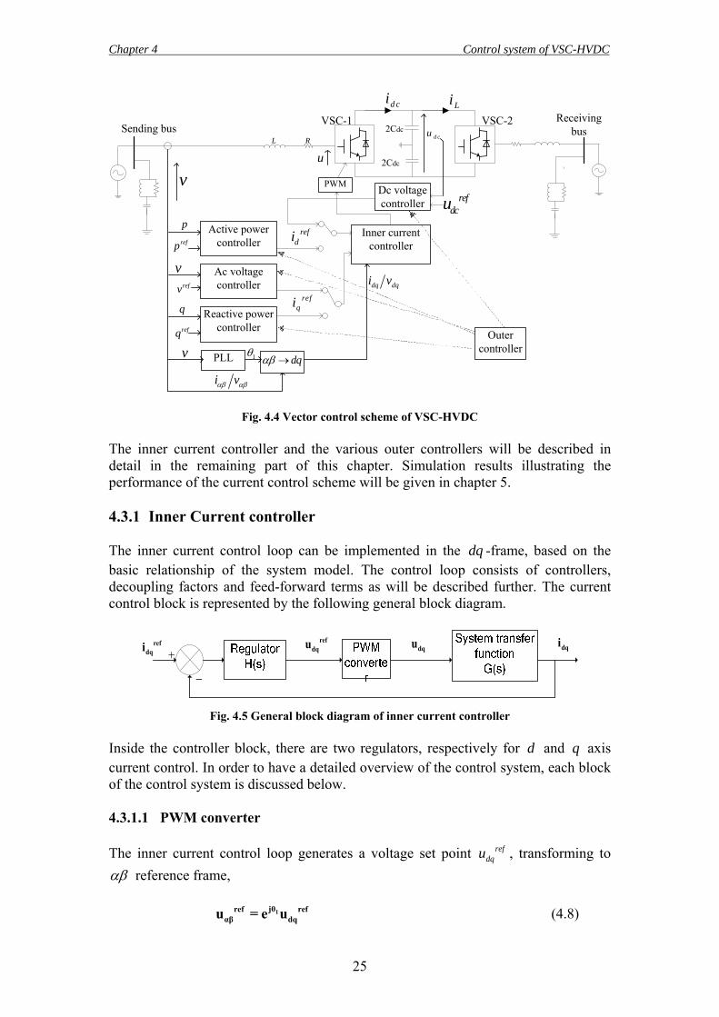
and dc dc dcp u i= (4.7) Eqns. (4.3, 4.5, 4.6, & 4.7) fully describe the VSC in Fig. 4.2. As can be seen, the transformation into rotating dq coordinate system leads to the possibility to control the two current components, d qi and i independently. Thus independent control of active and reactive power is possible; see Eqn. (4.5), assuming the PLL is performing well. As the vector control technique offers decoupled control of active and reactive power and fast dynamics, it makes the realization of system control in the form of a cascade structure possible, with two control loops in cascade: an outer control loop that provides the current set points and the inner current control loop described above. The outer controllers include the direct voltage controller, the active power controller, the reactive power controller, and the AC voltage controller, depending on the application. The reference value for active current can be provided by the direct voltage controller or the active power controller, while the reference value for reactive current is provided by AC voltage controller or reactive power controller. In all possible combinations of outer controllers, the direct voltage controller is always necessary to ensure an active power balance in the system. Active power taken out of the network must equal the active power fed into the network minus the losses in the DC system; any difference would mean that the direct voltage in the system will rapidly change to intolerable levels. Fig. 4.4 shows the various controllers of VSC-HVDC. The control system of VSC-2 is not shown explicitly, but is similar to that of VSC-1.
Chapter 4 Control system of VSC-HVDC
25
Active power controller
Ac voltage controller
Reactive power controller
Inner current controller
Dc voltage controller
PWM
PLL
2Cdc
2Cdc
Sending busReceiving
bus
Outer controller
d cu
d ci Li
refdcu
dq dqi vref
qi
refdi
i vαβ αβ
v
vrefv
q
refq
prefp
1θ dqαβ →
vu
L R
VSC-1 VSC-2
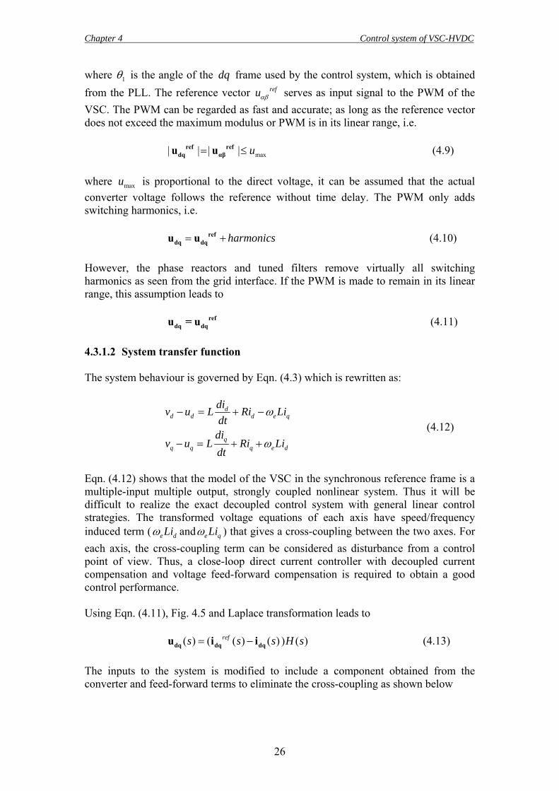
Fig. 4.4 Vector control scheme of VSC-HVDC The inner current controller and the various outer controllers will be described in detail in the remaining part of this chapter. Simulation results illustrating the performance of the current control scheme will be given in chapter 5. 4.3.1 Inner Current controller The inner current control loop can be implemented in the dq -frame, based on the basic relationship of the system model. The control loop consists of controllers, decoupling factors and feed-forward terms as will be described further. The current control block is represented by the following general block diagram.
−
+ref
dqi dqirefdqu dqu
Fig. 4.5 General block diagram of inner current controller
Inside the controller block, there are two regulators, respectively for d and q axis current control. In order to have a detailed overview of the control system, each block of the control system is discussed below. 4.3.1.1 PWM converter The inner current control loop generates a voltage set point ref
dqu , transforming to αβ reference frame, 1jθref ref
αβ dqu = e u (4.8)
Chapter 4 Control system of VSC-HVDC
26
where 1θ is the angle of the dq frame used by the control system, which is obtained from the PLL. The reference vector refuαβ serves as input signal to the PWM of the VSC. The PWM can be regarded as fast and accurate; as long as the reference vector does not exceed the maximum modulus or PWM is in its linear range, i.e. max| | | | u= ≤ref ref
dq αβu u (4.9)
where maxu is proportional to the direct voltage, it can be assumed that the actual converter voltage follows the reference without time delay. The PWM only adds switching harmonics, i.e. harmonics= +ref
dq dqu u (4.10) However, the phase reactors and tuned filters remove virtually all switching harmonics as seen from the grid interface. If the PWM is made to remain in its linear range, this assumption leads to ref
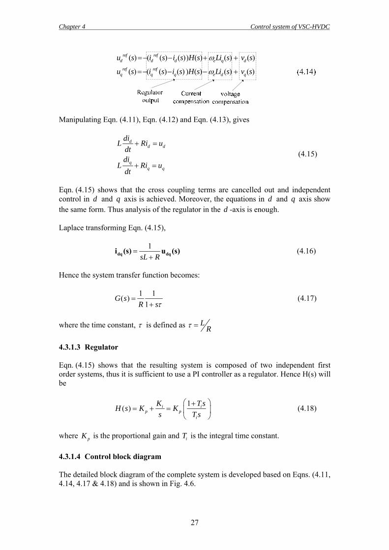
dq dqu = u (4.11) 4.3.1.2 System transfer function The system behaviour is governed by Eqn. (4.3) which is rewritten as:
dd d d e q
qq q q e d
div u L Ri Lidt
div u L Ri Li
dt
ω
ω
− = + −
− = + + (4.12)
Eqn. (4.12) shows that the model of the VSC in the synchronous reference frame is a multiple-input multiple output, strongly coupled nonlinear system. Thus it will be difficult to realize the exact decoupled control system with general linear control strategies. The transformed voltage equations of each axis have speed/frequency induced term ( e dLiω and e qLiω ) that gives a cross-coupling between the two axes. For each axis, the cross-coupling term can be considered as disturbance from a control point of view. Thus, a close-loop direct current controller with decoupled current compensation and voltage feed-forward compensation is required to obtain a good control performance. Using Eqn. (4.11), Fig. 4.5 and Laplace transformation leads to ( ) ( ( ) ( ) ) ( )refs s s H s= −dq dq dqu i i (4.13) The inputs to the system is modified to include a component obtained from the converter and feed-forward terms to eliminate the cross-coupling as shown below
Chapter 4 Control system of VSC-HVDC
27
( ) ( ( ) ( )) ( ) ( ) ( )
( ) ( ( ) ( ) ) ( ) ( ) ( )
ref refd d d e q d
ref refq q q e d q
u s i s i s H s Li s v s
u s i s i s H s Li s v s
ω
ω
=− − + +
=− − − +
Manipulating Eqn. (4.11), Eqn. (4.12) and Eqn. (4.13), gives
dd d
qq q
diL Ri udtdi
L Ri udt
+ =
+ = (4.15)
Eqn. (4.15) shows that the cross coupling terms are cancelled out and independent control in d and q axis is achieved. Moreover, the equations in d and q axis show the same form. Thus analysis of the regulator in the d -axis is enough. Laplace transforming Eqn. (4.15),
1sL R
=+dq dqi (s) u (s) (4.16)
Hence the system transfer function becomes:
1 1( )1
G sR sτ
=+
(4.17)
where the time constant, τ is defined as L
Rτ =
4.3.1.3 Regulator Eqn. (4.15) shows that the resulting system is composed of two independent first order systems, thus it is sufficient to use a PI controller as a regulator. Hence H(s) will be
1( ) i ip p
i
K T sH s K Ks T s
⎛ ⎞+= + = ⎜ ⎟
⎝ ⎠ (4.18)
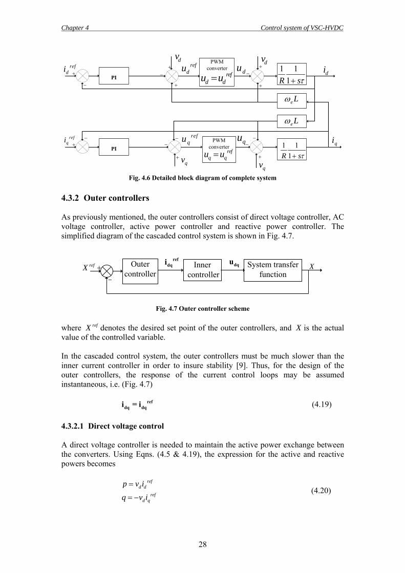
where pK is the proportional gain and iT is the integral time constant. 4.3.1.4 Control block diagram The detailed block diagram of the complete system is developed based on Eqns. (4.11, 4.14, 4.17 & 4.18) and is shown in Fig. 4.6.
Chapter 4 Control system of VSC-HVDC
28
PWMconverter ref
di diref
dudv
−
+PI −
+−
+
−+
PI−
+
refqi −
+
PWMconverter
+
− −
+
1 11R sτ+
1 11R sτ+
e Lω
e Lω
qvqv
dv
qiref
qu
du
qu
refd du u=
refq qu u=
Fig. 4.6 Detailed block diagram of complete system
4.3.2 Outer controllers As previously mentioned, the outer controllers consist of direct voltage controller, AC voltage controller, active power controller and reactive power controller. The simplified diagram of the cascaded control system is shown in Fig. 4.7.
−+ Outer
controllerInner
controller System transfer
functionrefX X
refdqi dqu
Fig. 4.7 Outer controller scheme
where refX denotes the desired set point of the outer controllers, and X is the actual value of the controlled variable. In the cascaded control system, the outer controllers must be much slower than the inner current controller in order to insure stability [9]. Thus, for the design of the outer controllers, the response of the current control loops may be assumed instantaneous, i.e. (Fig. 4.7) ref
dq dqi = i (4.19) 4.3.2.1 Direct voltage control A direct voltage controller is needed to maintain the active power exchange between the converters. Using Eqns. (4.5 & 4.19), the expression for the active and reactive powers becomes
ref
d d
refd q
p v i
q v i
=
= − (4.20)
Chapter 4 Control system of VSC-HVDC
29
Neglecting losses in the converter and phase reactor, equating the power on the AC and DC sides of the converter using Eqns. (4.7 & 4.20):
refddc d
dc
vi iu
= (3.21)
Any unbalance between AC and DC powers leads to a change in voltage over the DC link capacitor, equating Eqn. (4.6) and Eqn. (4.21)
dc ddc d L
dc
du vC i idt u
= − (4.22)
We see that Eqn. (4.22) is non-linear with respect to dcu . Linearizing Eqn. (4.22)
around steady state operating point as outlined in [8] and considering Li as a
disturbance signal, the transfer function from dcu to di becomes
0
1( ) d
dc dc
vG su s C
= (4.23)
where 0dcu is the steady state DC-link capacitor voltage. Transfer function, ( )G s , has a pole at the origin, thus it will be difficult to control it. Introducing an inner feedback loop for active power damping as outlined in [17], 'ref
d d a dci i G u= − (4.24) Substituting Eqn. (4.24) into Eqn. (4.22) gives
'
0
( )dc ddc d a dc
dc
du vC i G udt u
= − (4.25)
The Laplace transformation from '
di to dcu becomes
' 0
0
( )( )
d dc
dc a d dc
v uG ssC G v u
=+
(4.26)
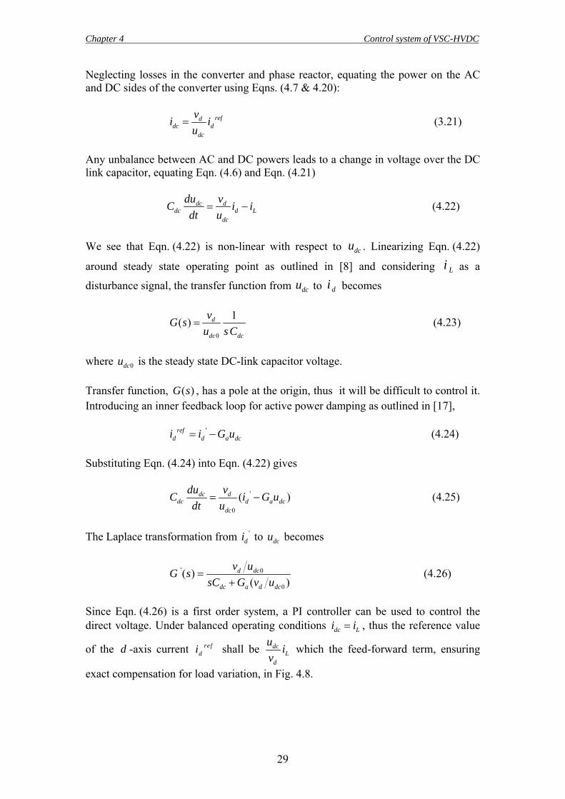
Since Eqn. (4.26) is a first order system, a PI controller can be used to control the direct voltage. Under balanced operating conditions dc Li i= , thus the reference value
of the d -axis current refdi shall be dc
Ld
u iv
which the feed-forward term, ensuring
exact compensation for load variation, in Fig. 4.8.
Chapter 4 Control system of VSC-HVDC
30
−
+ref
dcu 'di
d cL
d
u iv
dcu aG
−
+ refdi
maxi
maxi−
limdi
Fig. 4.8 Direct voltage controller structure
4.3.2.2 Active and reactive power control If dv in Eqn. (4.20) is assumed to be constant, then the active and reactive powers will be correlated with the active and reactive current references respectively. The simplest method to control the active and reactive powers will therefore be an open-loop controller, Eqn. (4.27).
refref
dd
refref
qd
Piv
qiv
=
= − (4.27)
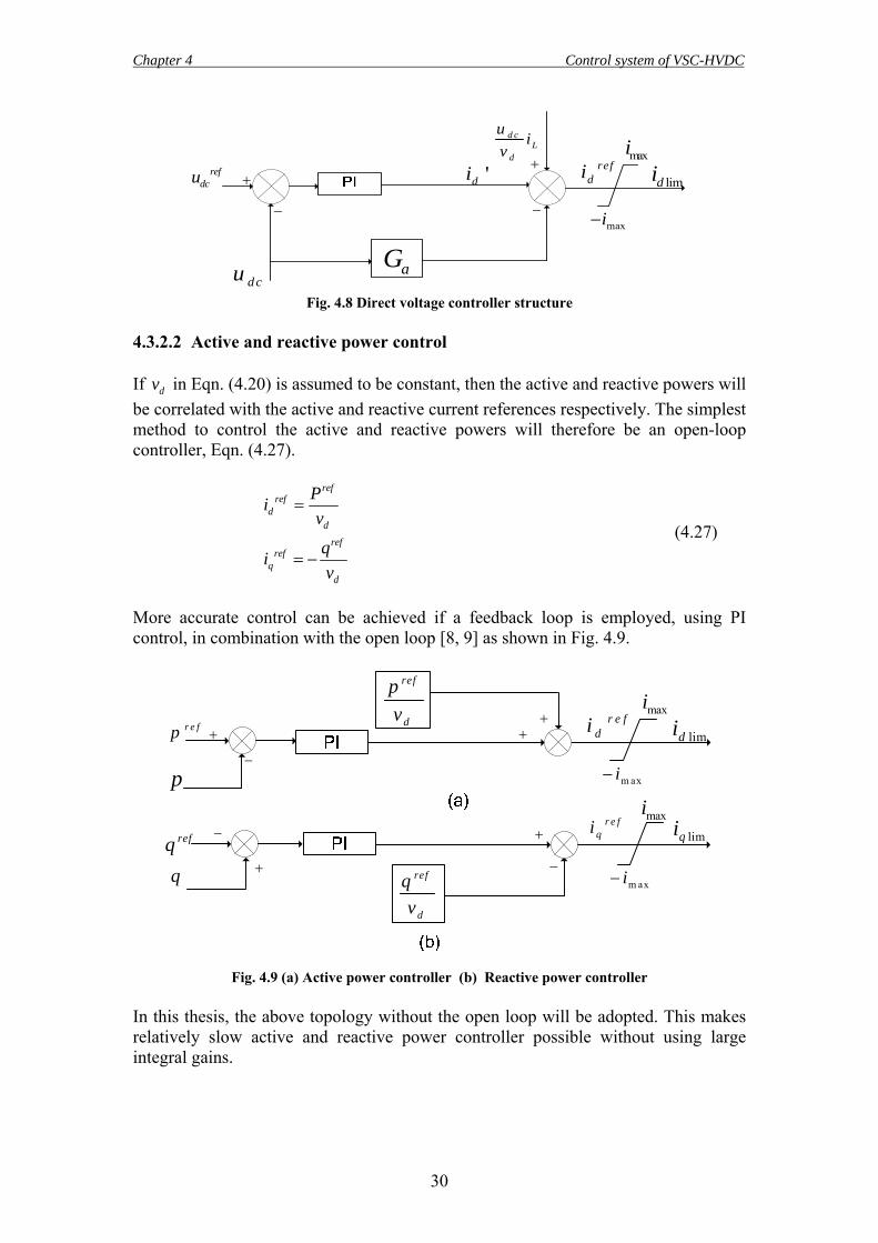
More accurate control can be achieved if a feedback loop is employed, using PI control, in combination with the open loop [8, 9] as shown in Fig. 4.9.
−
+r e fp
ref
d
pv
p
r e fdi+
−
+
refqref
d
qv
q
r e fqi
−
+
+
maxi
m axi−
maxi
m axi−
limqi
limdi
Fig. 4.9 (a) Active power controller (b) Reactive power controller In this thesis, the above topology without the open loop will be adopted. This makes relatively slow active and reactive power controller possible without using large integral gains.
Chapter 4 Control system of VSC-HVDC
31
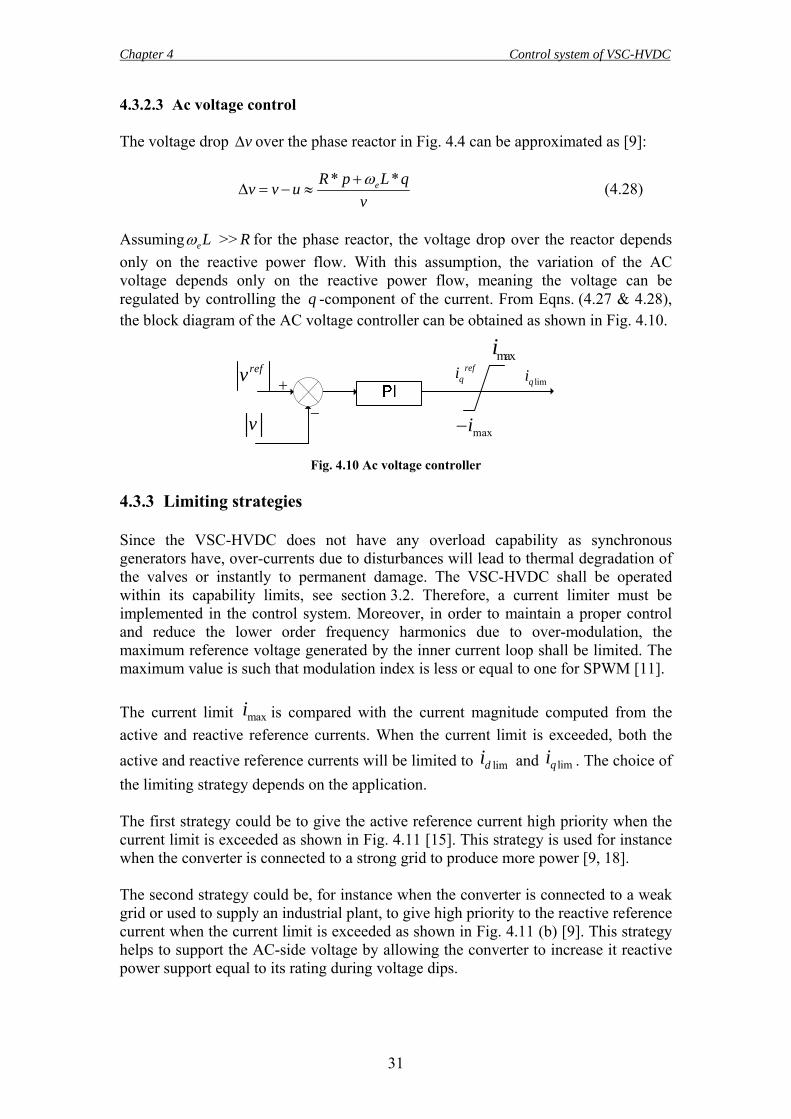
4.3.2.3 Ac voltage control The voltage drop vΔ over the phase reactor in Fig. 4.4 can be approximated as [9]:
* *eR p L qv v uvω+
Δ = − ≈ (4.28)
Assuming eLω >> R for the phase reactor, the voltage drop over the reactor depends only on the reactive power flow. With this assumption, the variation of the AC voltage depends only on the reactive power flow, meaning the voltage can be regulated by controlling the q -component of the current. From Eqns. (4.27 & 4.28), the block diagram of the AC voltage controller can be obtained as shown in Fig. 4.10.
−
+refv ref
qimaxi
maxi−
limqi
v
Fig. 4.10 Ac voltage controller 4.3.3 Limiting strategies Since the VSC-HVDC does not have any overload capability as synchronous generators have, over-currents due to disturbances will lead to thermal degradation of the valves or instantly to permanent damage. The VSC-HVDC shall be operated within its capability limits, see section 3.2. Therefore, a current limiter must be implemented in the control system. Moreover, in order to maintain a proper control and reduce the lower order frequency harmonics due to over-modulation, the maximum reference voltage generated by the inner current loop shall be limited. The maximum value is such that modulation index is less or equal to one for SPWM [11]. The current limit maxi is compared with the current magnitude computed from the active and reactive reference currents. When the current limit is exceeded, both the active and reactive reference currents will be limited to limdi and limqi . The choice of the limiting strategy depends on the application. The first strategy could be to give the active reference current high priority when the current limit is exceeded as shown in Fig. 4.11 [15]. This strategy is used for instance when the converter is connected to a strong grid to produce more power [9, 18]. The second strategy could be, for instance when the converter is connected to a weak grid or used to supply an industrial plant, to give high priority to the reactive reference current when the current limit is exceeded as shown in Fig. 4.11 (b) [9]. This strategy helps to support the AC-side voltage by allowing the converter to increase it reactive power support equal to its rating during voltage dips.
Chapter 4 Control system of VSC-HVDC
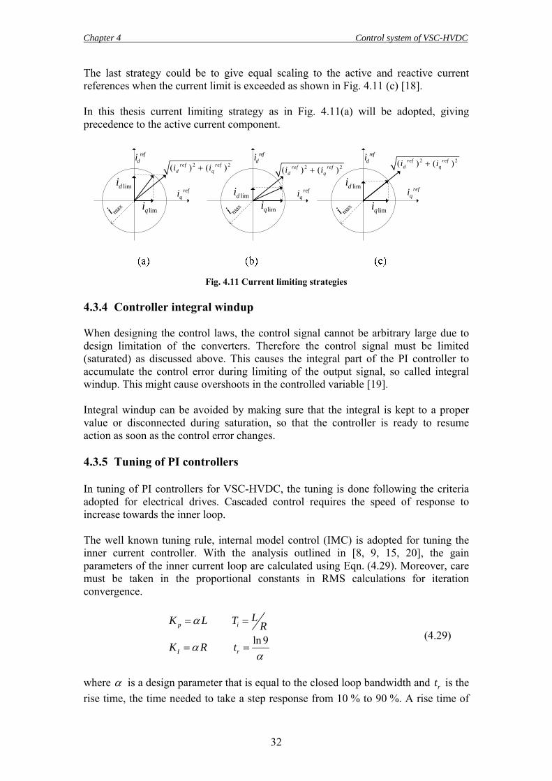
32
The last strategy could be to give equal scaling to the active and reactive current references when the current limit is exceeded as shown in Fig. 4.11 (c) [18]. In this thesis current limiting strategy as in Fig. 4.11(a) will be adopted, giving precedence to the active current component.
limdi
refdi
refqi
maxi limqilimdi
refdi
refqi
maxi limqi
limdi
refdi
2 2( ) ( )ref refd qi i+
refqi
maxi limqi
2 2( ) ( )ref refd qi i+
2 2( ) ( )ref refd qi i+
Fig. 4.11 Current limiting strategies
4.3.4 Controller integral windup When designing the control laws, the control signal cannot be arbitrary large due to design limitation of the converters. Therefore the control signal must be limited (saturated) as discussed above. This causes the integral part of the PI controller to accumulate the control error during limiting of the output signal, so called integral windup. This might cause overshoots in the controlled variable [19]. Integral windup can be avoided by making sure that the integral is kept to a proper value or disconnected during saturation, so that the controller is ready to resume action as soon as the control error changes. 4.3.5 Tuning of PI controllers In tuning of PI controllers for VSC-HVDC, the tuning is done following the criteria adopted for electrical drives. Cascaded control requires the speed of response to increase towards the inner loop. The well known tuning rule, internal model control (IMC) is adopted for tuning the inner current controller. With the analysis outlined in [8, 9, 15, 20], the gain parameters of the inner current loop are calculated using Eqn. (4.29). Moreover, care must be taken in the proportional constants in RMS calculations for iteration convergence.
ln 9p i
I r
LK L T R
K R t
α
αα
= =
= = (4.29)
where α is a design parameter that is equal to the closed loop bandwidth and rt is the rise time, the time needed to take a step response from 10 % to 90 %. A rise time of
Chapter 4 Control system of VSC-HVDC
33
rt =2 ms, equivalentlyα =1098 rad/s will be used for the inner current loop. This is in agreement with the phase reactor inductance value requirement of Section 3.6, Eqn. (3.10). However, the performance of the control system will get better if the inner loop is made to respond instantaneous. But in reality instantaneous response means usually infinite amplification of noise. IMC is also used to tune the direct voltage controller. The gain parameters are calculated based on analysis outlined in [9, 15, 17] where the equations are reproduced here as Eqn. (4.30).
2
p d dc a d dc
I d dc
K C G C
K C
α α
α
= =
= (4.31)
where dα =220 rad/ s is used as an initial value. The actual gains used are a bit modified from the ones calculated based on Eqn. (4.30) to get the desired response time, slower than the inner current controller. For the AC voltage and Reactive power controllers, there are no general tuning rules as the controller gain depends on the network impedance [20]. Therefore it is made via trial and error to get a reasonable speed of response, slower than the inner current and direct voltage controllers.
34
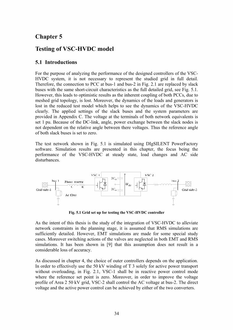
Chapter 5 Testing of VSC-HVDC model 5.1 Introductions For the purpose of analyzing the performance of the designed controllers of the VSC-HVDC system, it is not necessary to represent the studied grid in full detail. Therefore, the connection to PCC at bus-1 and bus-2 in Fig. 2.1 are replaced by slack buses with the same short-circuit characteristics as the full detailed grid, see Fig. 5.1. However, this leads to optimistic results as the inherent coupling of both PCCs, due to meshed grid topology, is lost. Moreover, the dynamics of the loads and generators is lost in the reduced test model which helps to see the dynamics of the VSC-HVDC clearly. The applied settings of the slack buses and the system parameters are provided in Appendix C. The voltage at the terminals of both network equivalents is set 1 pu. Because of the DC-link, angle, power exchange between the slack nodes is not dependent on the relative angle between there voltages. Thus the reference angle of both slack buses is set to zero. The test network shown in Fig. 5.1 is simulated using DIgSILENT PowerFactory software. Simulation results are presented in this chapter, the focus being the performance of the VSC-HVDC at steady state, load changes and AC side disturbances.
dcu2 dcC
2 dcC
Fig. 5.1 Grid set up for testing the VSC-HVDC controller As the intent of this thesis is the study of the integration of VSC-HVDC to alleviate network constraints in the planning stage, it is assumed that RMS simulations are sufficiently detailed. However, EMT simulations are made for some special study cases. Moreover switching actions of the valves are neglected in both EMT and RMS simulations. It has been shown in [9] that this assumption does not result in a considerable loss of accuracy. As discussed in chapter 4, the choice of outer controllers depends on the application. In order to effectively use the 50 kV winding of T 3 solely for active power transport without overloading, in Fig. 2.1, VSC-1 shall be in reactive power control mode where the reference set point is zero. Moreover, in order to improve the voltage profile of Area 2 50 kV grid, VSC-2 shall control the AC voltage at bus-2. The direct voltage and the active power control can be achieved by either of the two converters.
Chapter 5 Testing of VSC-HVDC model controller
35
Thus, we have two possible control strategies: Strategy 1: VSC-1 controls the reactive power and the active power VSC-2 controls the AC voltage and the direct voltage Strategy 2: VSC-1 controls the reactive power and the direct voltage VSC-2 controls the active power and the AC voltage The choice between the two strategies depends mainly on two factors. Firstly, the accurate control of the active power exchange between the AC and DC sides without implementing loss dependent active power set point in the control system to avoid overloading of T 3, 50 kV winding in Fig. 2.1, Strategy-2 will be more appropriate than Strategy-1. Area 2 consists of cables of longer length in its distribution and sub-transmission grid than Area 1. In addition, there are overhead lines in Area 2 but not in Area 1. Thus the frequency of disturbances in Area 2 is expected to be higher than in Area 1. Furthermore, disturbances in Area 2 cause larger voltage dips at bus-2 than disturbances in Area 1 cause at bus 8. As voltage dips hinder the performance of the VSC-HVDC controllers, the preferred strategy will be to have VSC-1 control the direct voltage, which is Strategy-2.
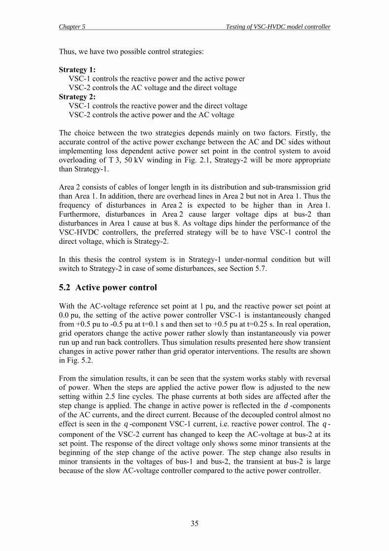
In this thesis the control system is in Strategy-1 under-normal condition but will switch to Strategy-2 in case of some disturbances, see Section 5.7. 5.2 Active power control With the AC-voltage reference set point at 1 pu, and the reactive power set point at 0.0 pu, the setting of the active power controller VSC-1 is instantaneously changed from +0.5 pu to -0.5 pu at t=0.1 s and then set to +0.5 pu at t=0.25 s. In real operation, grid operators change the active power rather slowly than instantaneously via power run up and run back controllers. Thus simulation results presented here show transient changes in active power rather than grid operator interventions. The results are shown in Fig. 5.2. From the simulation results, it can be seen that the system works stably with reversal of power. When the steps are applied the active power flow is adjusted to the new setting within 2.5 line cycles. The phase currents at both sides are affected after the step change is applied. The change in active power is reflected in the d -components of the AC currents, and the direct current. Because of the decoupled control almost no effect is seen in the q -component VSC-1 current, i.e. reactive power control. The q -component of the VSC-2 current has changed to keep the AC-voltage at bus-2 at its set point. The response of the direct voltage only shows some minor transients at the beginning of the step change of the active power. The step change also results in minor transients in the voltages of bus-1 and bus-2, the transient at bus-2 is large because of the slow AC-voltage controller compared to the active power controller.
Chapter 5 Testing of VSC-HVDC model controller
36
0.400.300.200.100.00 [s]
1.02
1.01
1.00
0.99
bus-1: Voltage Magnitude in p.u.bus-2: Voltage Magnitude in p.u.
0.400.300.200.100.00 [s]
1.02
1.01
1.00
0.99
Dc Bus: Vdc
0.400.300.200.100.00 [s]
0.75
0.50
0.25
0.00
-0.25
-0.50
-0.75
VSC-1: Current, q-Axis in p.u.VSC-1: Current, d-Axis in p.u.VSC-1: Phase Current, Magnitude in p.u.
0.400.300.200.100.00 [s]
0.75
0.50
0.25
0.00
-0.25
-0.50
-0.75
Grid side-1: Active Power in p.u.Grid side-2: Active Power in p.u.
0.400.300.200.100.00 [s]
0.75
0.50
0.25
0.00
-0.25
-0.50
-0.75
VSC-2: Current, d-Axis in p.u.VSC-2: Current, q-Axis in p.u.Dc Bus: current, idc in p.u.
0.400.300.200.100.00 [s]
0.10
0.00
-0.10
-0.20
-0.30
-0.40
Grid side-1: Reactive Power in p.u.Grid side-2: Reactive Power in p.u.
Fig. 5.2 Transient responses for a step change in active power 5.3 Reactive power control In this case, AC-voltage reference is held at 1 pu. The system is initially operated with reactive power reference of +0.3 pu and active power reference of +0.5 pu. At t=0.1 s, the reactive power reference is set to -0.3 pu and then set back to +0.3 pu at t=0.25 s. The response of the system is shown in Fig. 5.3.
0.400.300.200.100.00 [s]
1.05
1.04
1.03
1.02
1.01
1.00
0.99
bus-1: Voltage Magnitude in p.u.bus-2: Voltage Magnitude in p.u.
0.400.300.200.100.00 [s]
1.0015
1.0010
1.0005
1.0000
0.9995
0.9990
Dc Bus: Vdc
0.400.300.200.100.00 [s]
0.75
0.50
0.25
0.00
-0.25
-0.50
-0.75
Grid side-1: Active Power in p.u.Grid side-2: Active Power in p.u.
0.400.300.200.100.00 [s]
0.90
0.60
0.30
0.00
-0.30
-0.60
VSC-1: Current, q-Axis in p.u.VSC-1: Current, d-Axis in p.u.VSC-1: Phase Current, Magnitude in p.u.
0.400.300.200.100.00 [s]
0.60
0.50
0.40
0.30
0.20
0.10
0.00
VSC-2: Current, d-Axis in p.u.VSC-2: Current, q-Axis in p.u.Dc Bus: current, idc in p.u.
0.400.300.200.100.00 [s]
0.40
0.20
0.00
-0.20
-0.40
Grid side-1: Reactive Power in p.u.Grid side-2: Reactive Power in p.u.
Fig. 5.3 Transient responses for a step change in reactive power
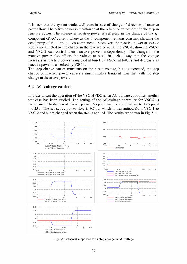
Chapter 5 Testing of VSC-HVDC model controller
37
It is seen that the system works well even in case of change of direction of reactive power flow. The active power is maintained at the reference values despite the step in reactive power. The change in reactive power is reflected in the change of the q -component of AC current, where as the d -component remains constant, showing the decoupling of the d and q-axis components. Moreover, the reactive power at VSC-2 side is not affected by the change in the reactive power at the VSC-1, showing VSC-1 and VSC-2 can control their reactive powers independently. The change in the reactive power also affects the voltage at bus-1 in such a way that the voltage increases as reactive power is injected at bus-1 by VSC-1 at t=0.1 s and decreases as reactive power is absorbed by VSC-1.
The step change causes transients on the direct voltage, but, as expected, the step change of reactive power causes a much smaller transient than that with the step change in the active power. 5.4 AC voltage control In order to test the operation of the VSC-HVDC as an AC-voltage controller, another test case has been studied. The setting of the AC-voltage controller for VSC-2 is instantaneously decreased from 1 pu to 0.95 pu at t=0.1 s and then set to 1.05 pu at t=0.25 s. The set active power flow is 0.5 pu, which is transmitted from VSC-1 to VSC-2 and is not changed when the step is applied. The results are shown in Fig. 5.4.
0.400.300.200.100.00 [s]
1.02
1.01
1.00
0.99
Dc Bus: Vdc
0.400.300.200.100.00 [s]
1.10
1.06
1.02
0.98
0.94
0.90
bus-1: Voltage Magnitude in p.u.bus-2: Voltage Magnitude in p.u.
0.400.300.200.100.00 [s]
0.75
0.50
0.25
0.00
-0.25
-0.50
-0.75
Grid side-1: Active Power in p.u.Grid side-2: Active Power in p.u.
0.400.300.200.100.00 [s]
0.75
0.50
0.25
0.00
-0.25
-0.50
-0.75
VSC-1: Current, q-Axis in p.u.VSC-1: Current, d-Axis in p.u.VSC-1: Phase Current, Magnitude in p.u.
0.400.300.200.100.00 [s]
0.60
0.40
0.20
0.00
-0.20
-0.40
VSC-2: Current, d-Axis in p.u.VSC-2: Current, q-Axis in p.u.Dc Bus: current, idc in p.u.
0.400.300.200.100.00 [s]
0.40
0.20
0.00
-0.20
-0.40
-0.60
Grid side-1: Reactive Power in p.u.Grid side-2: Reactive Power in p.u.
0.400.300.200.100.00 [s]
0.60
0.40
0.20
0.00
-0.20
-0.40
VSC-1: Reactive power in p.u.VSC-2: Reactive power in p.u.
Fig. 5.4 Transient responses for a step change in AC voltage
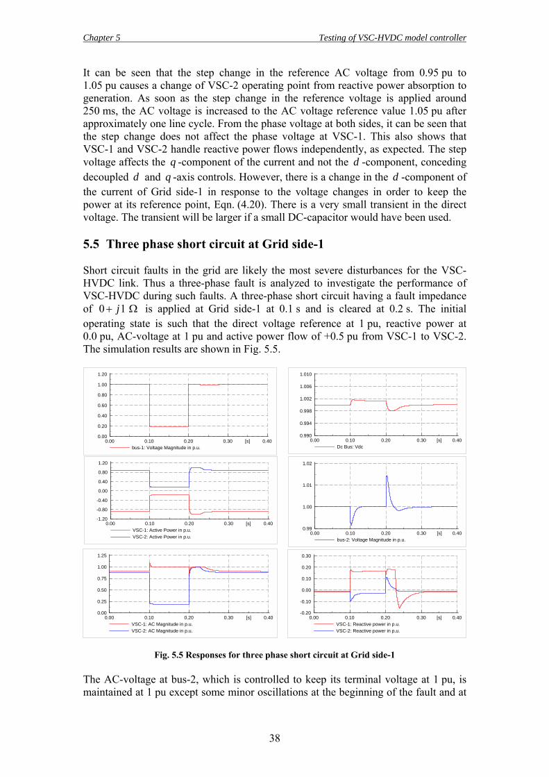
Chapter 5 Testing of VSC-HVDC model controller
38
It can be seen that the step change in the reference AC voltage from 0.95 pu to 1.05 pu causes a change of VSC-2 operating point from reactive power absorption to generation. As soon as the step change in the reference voltage is applied around 250 ms, the AC voltage is increased to the AC voltage reference value 1.05 pu after approximately one line cycle. From the phase voltage at both sides, it can be seen that the step change does not affect the phase voltage at VSC-1. This also shows that VSC-1 and VSC-2 handle reactive power flows independently, as expected. The step voltage affects the q -component of the current and not the d -component, conceding decoupled d and q -axis controls. However, there is a change in the d -component of the current of Grid side-1 in response to the voltage changes in order to keep the power at its reference point, Eqn. (4.20). There is a very small transient in the direct voltage. The transient will be larger if a small DC-capacitor would have been used. 5.5 Three phase short circuit at Grid side-1 Short circuit faults in the grid are likely the most severe disturbances for the VSC-HVDC link. Thus a three-phase fault is analyzed to investigate the performance of VSC-HVDC during such faults. A three-phase short circuit having a fault impedance of 0 1j+ Ω is applied at Grid side-1 at 0.1 s and is cleared at 0.2 s. The initial operating state is such that the direct voltage reference at 1 pu, reactive power at 0.0 pu, AC-voltage at 1 pu and active power flow of +0.5 pu from VSC-1 to VSC-2. The simulation results are shown in Fig. 5.5.
0.400.300.200.100.00 [s]
1.20
0.80
0.40
0.00
-0.40
-0.80
-1.20
VSC-1: Active Power in p.u.VSC-2: Active Power in p.u.
0.400.300.200.100.00 [s]
1.20
1.00
0.80
0.60
0.40
0.20
0.00
bus-1: Voltage Magnitude in p.u.
0.400.300.200.100.00 [s]
0.30
0.20
0.10
0.00
-0.10
-0.20
VSC-1: Reactive power in p.u.VSC-2: Reactive power in p.u.
0.400.300.200.100.00 [s]
1.010
1.006
1.002
0.998
0.994
0.990
Dc Bus: Vdc
0.400.300.200.100.00 [s]
1.02
1.01
1.00
0.99
bus-2: Voltage Magnitude in p.u.
0.400.300.200.100.00 [s]
1.25
1.00
0.75
0.50
0.25
0.00
VSC-1: AC Magnitude in p.u.VSC-2: AC Magnitude in p.u.
Fig. 5.5 Responses for three phase short circuit at Grid side-1
The AC-voltage at bus-2, which is controlled to keep its terminal voltage at 1 pu, is maintained at 1 pu except some minor oscillations at the beginning of the fault and at
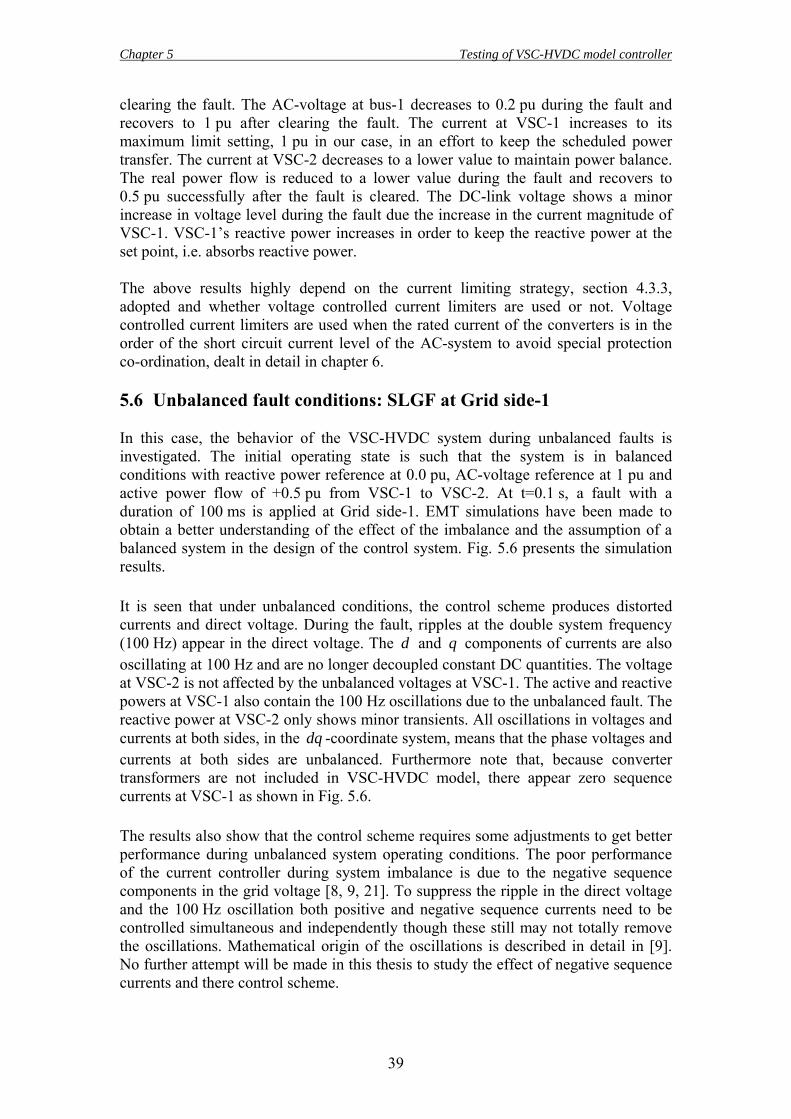
Chapter 5 Testing of VSC-HVDC model controller
39
clearing the fault. The AC-voltage at bus-1 decreases to 0.2 pu during the fault and recovers to 1 pu after clearing the fault. The current at VSC-1 increases to its maximum limit setting, 1 pu in our case, in an effort to keep the scheduled power transfer. The current at VSC-2 decreases to a lower value to maintain power balance. The real power flow is reduced to a lower value during the fault and recovers to 0.5 pu successfully after the fault is cleared. The DC-link voltage shows a minor increase in voltage level during the fault due the increase in the current magnitude of VSC-1. VSC-1’s reactive power increases in order to keep the reactive power at the set point, i.e. absorbs reactive power. The above results highly depend on the current limiting strategy, section 4.3.3, adopted and whether voltage controlled current limiters are used or not. Voltage controlled current limiters are used when the rated current of the converters is in the order of the short circuit current level of the AC-system to avoid special protection co-ordination, dealt in detail in chapter 6. 5.6 Unbalanced fault conditions: SLGF at Grid side-1 In this case, the behavior of the VSC-HVDC system during unbalanced faults is investigated. The initial operating state is such that the system is in balanced conditions with reactive power reference at 0.0 pu, AC-voltage reference at 1 pu and active power flow of +0.5 pu from VSC-1 to VSC-2. At t=0.1 s, a fault with a duration of 100 ms is applied at Grid side-1. EMT simulations have been made to obtain a better understanding of the effect of the imbalance and the assumption of a balanced system in the design of the control system. Fig. 5.6 presents the simulation results. It is seen that under unbalanced conditions, the control scheme produces distorted currents and direct voltage. During the fault, ripples at the double system frequency (100 Hz) appear in the direct voltage. The d and q components of currents are also oscillating at 100 Hz and are no longer decoupled constant DC quantities. The voltage at VSC-2 is not affected by the unbalanced voltages at VSC-1. The active and reactive powers at VSC-1 also contain the 100 Hz oscillations due to the unbalanced fault. The reactive power at VSC-2 only shows minor transients. All oscillations in voltages and currents at both sides, in the dq -coordinate system, means that the phase voltages and currents at both sides are unbalanced. Furthermore note that, because converter transformers are not included in VSC-HVDC model, there appear zero sequence currents at VSC-1 as shown in Fig. 5.6. The results also show that the control scheme requires some adjustments to get better performance during unbalanced system operating conditions. The poor performance of the current controller during system imbalance is due to the negative sequence components in the grid voltage [8, 9, 21]. To suppress the ripple in the direct voltage and the 100 Hz oscillation both positive and negative sequence currents need to be controlled simultaneous and independently though these still may not totally remove the oscillations. Mathematical origin of the oscillations is described in detail in [9]. No further attempt will be made in this thesis to study the effect of negative sequence currents and there control scheme.
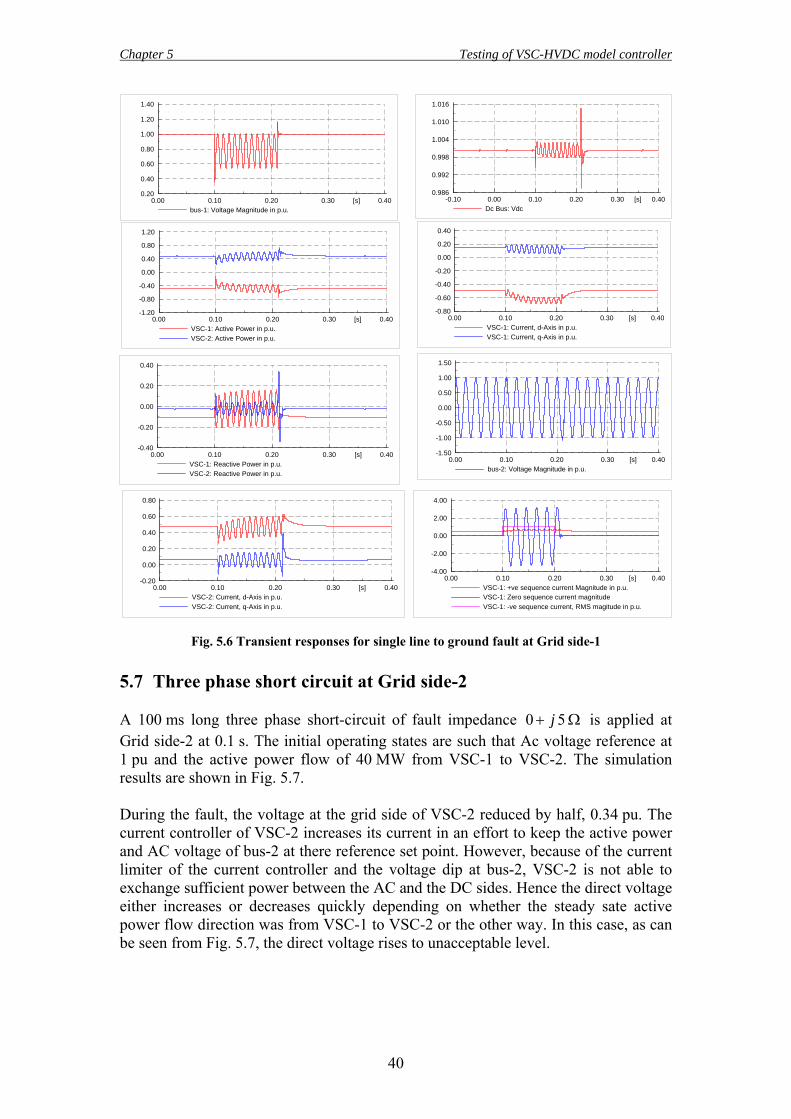
Chapter 5 Testing of VSC-HVDC model controller
40
0.400.300.200.100.00 [s]
1.20
0.80
0.40
0.00
-0.40
-0.80
-1.20
VSC-1: Active Power in p.u.VSC-2: Active Power in p.u.
0.400.300.200.100.00 [s]
1.40
1.20
1.00
0.80
0.60
0.40
0.20
bus-1: Voltage Magnitude in p.u.0.400.300.200.100.00-0.10 [s]
1.016
1.010
1.004
0.998
0.992
0.986
Dc Bus: Vdc
0.400.300.200.100.00 [s]
0.40
0.20
0.00
-0.20
-0.40
VSC-1: Reactive Power in p.u.VSC-2: Reactive Power in p.u.
0.400.300.200.100.00 [s]
0.40
0.20
0.00
-0.20
-0.40
-0.60
-0.80
VSC-1: Current, d-Axis in p.u.VSC-1: Current, q-Axis in p.u.
0.400.300.200.100.00 [s]
1.50
1.00
0.50
0.00
-0.50
-1.00
-1.50
bus-2: Voltage Magnitude in p.u.
0.400.300.200.100.00 [s]
0.80
0.60
0.40
0.20
0.00
-0.20
VSC-2: Current, d-Axis in p.u.VSC-2: Current, q-Axis in p.u.
0.400.300.200.100.00 [s]
4.00
2.00
0.00
-2.00
-4.00
VSC-1: +ve sequence current Magnitude in p.u.VSC-1: Zero sequence current magnitudeVSC-1: -ve sequence current, RMS magitude in p.u.
Fig. 5.6 Transient responses for single line to ground fault at Grid side-1
5.7 Three phase short circuit at Grid side-2 A 100 ms long three phase short-circuit of fault impedance 0 5j+ Ω is applied at Grid side-2 at 0.1 s. The initial operating states are such that Ac voltage reference at 1 pu and the active power flow of 40 MW from VSC-1 to VSC-2. The simulation results are shown in Fig. 5.7. During the fault, the voltage at the grid side of VSC-2 reduced by half, 0.34 pu. The current controller of VSC-2 increases its current in an effort to keep the active power and AC voltage of bus-2 at there reference set point. However, because of the current limiter of the current controller and the voltage dip at bus-2, VSC-2 is not able to exchange sufficient power between the AC and the DC sides. Hence the direct voltage either increases or decreases quickly depending on whether the steady sate active power flow direction was from VSC-1 to VSC-2 or the other way. In this case, as can be seen from Fig. 5.7, the direct voltage rises to unacceptable level.
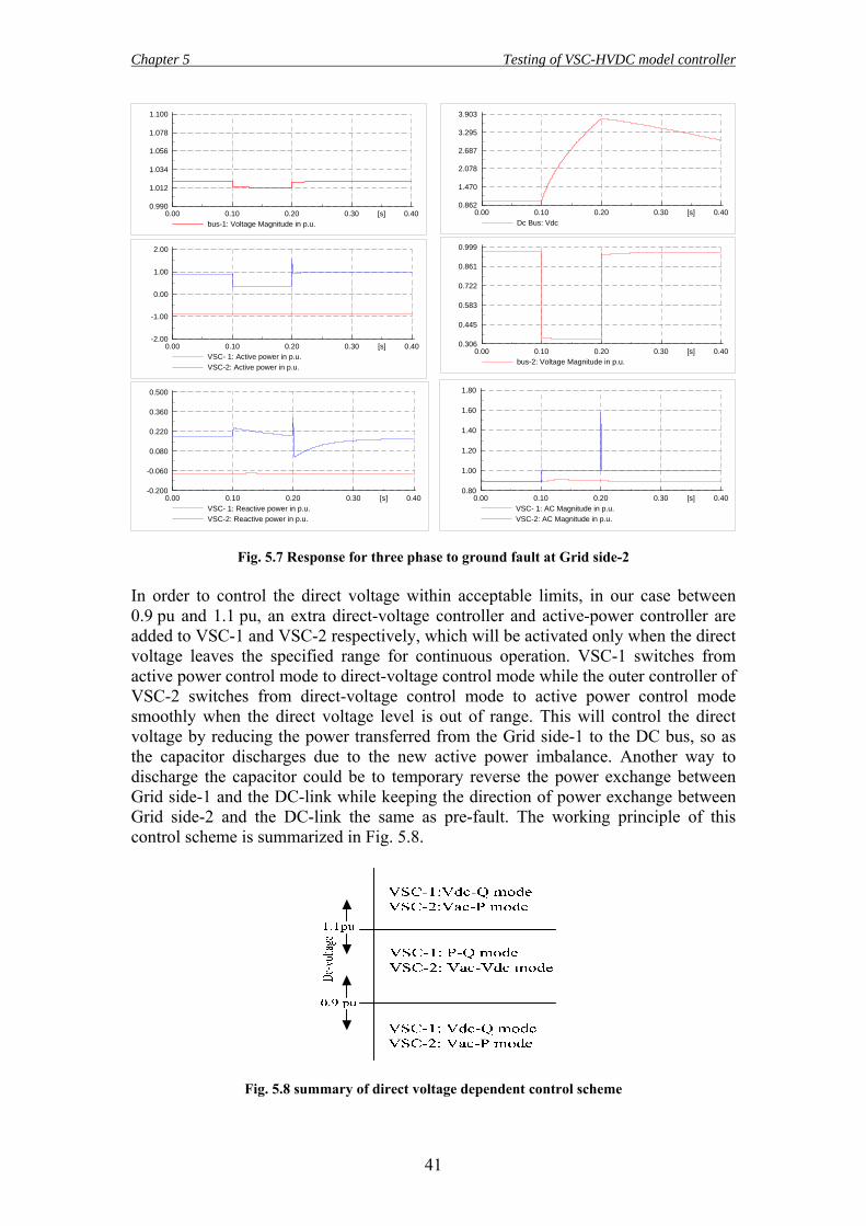
Chapter 5 Testing of VSC-HVDC model controller
41
0.400.300.200.100.00 [s]
1.80
1.60
1.40
1.20
1.00
0.80
VSC- 1: AC Magnitude in p.u.VSC-2: AC Magnitude in p.u.
0.400.300.200.100.00 [s]
0.500
0.360
0.220
0.080
-0.060
-0.200
VSC- 1: Reactive power in p.u.VSC-2: Reactive power in p.u.
0.400.300.200.100.00 [s]
3.903
3.295
2.687
2.078
1.470
0.862
Dc Bus: Vdc
0.400.300.200.100.00 [s]
0.999
0.861
0.722
0.583
0.445
0.306
bus-2: Voltage Magnitude in p.u.
0.400.300.200.100.00 [s]
2.00
1.00
0.00
-1.00
-2.00
VSC- 1: Active power in p.u.VSC-2: Active power in p.u.
0.400.300.200.100.00 [s]
1.100
1.078
1.056
1.034
1.012
0.990
bus-1: Voltage Magnitude in p.u.
Fig. 5.7 Response for three phase to ground fault at Grid side-2 In order to control the direct voltage within acceptable limits, in our case between 0.9 pu and 1.1 pu, an extra direct-voltage controller and active-power controller are added to VSC-1 and VSC-2 respectively, which will be activated only when the direct voltage leaves the specified range for continuous operation. VSC-1 switches from active power control mode to direct-voltage control mode while the outer controller of VSC-2 switches from direct-voltage control mode to active power control mode smoothly when the direct voltage level is out of range. This will control the direct voltage by reducing the power transferred from the Grid side-1 to the DC bus, so as the capacitor discharges due to the new active power imbalance. Another way to discharge the capacitor could be to temporary reverse the power exchange between Grid side-1 and the DC-link while keeping the direction of power exchange between Grid side-2 and the DC-link the same as pre-fault. The working principle of this control scheme is summarized in Fig. 5.8.
Fig. 5.8 summary of direct voltage dependent control scheme
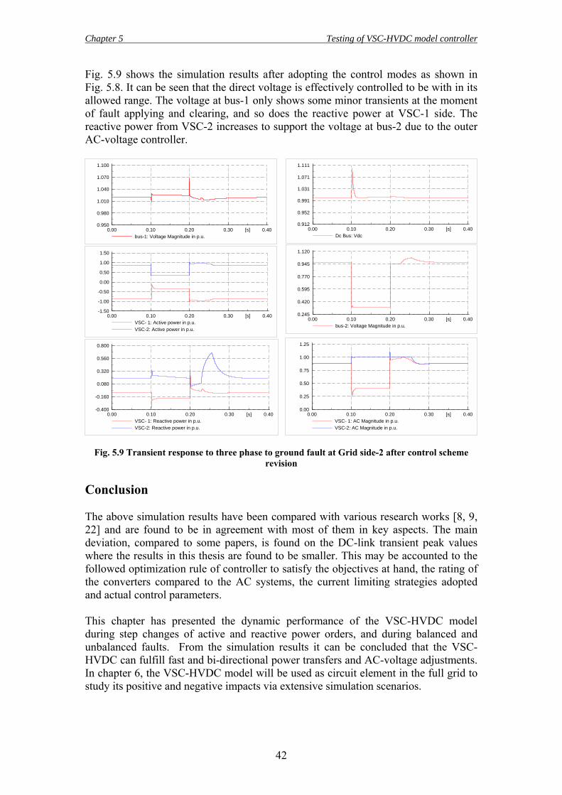
Chapter 5 Testing of VSC-HVDC model controller
42
Fig. 5.9 shows the simulation results after adopting the control modes as shown in Fig. 5.8. It can be seen that the direct voltage is effectively controlled to be with in its allowed range. The voltage at bus-1 only shows some minor transients at the moment of fault applying and clearing, and so does the reactive power at VSC-1 side. The reactive power from VSC-2 increases to support the voltage at bus-2 due to the outer AC-voltage controller.
0.400.300.200.100.00 [s]
1.25
1.00
0.75
0.50
0.25
0.00
VSC- 1: AC Magnitude in p.u.VSC-2: AC Magnitude in p.u.
0.400.300.200.100.00 [s]
0.800
0.560
0.320
0.080
-0.160
-0.400
VSC- 1: Reactive power in p.u.VSC-2: Reactive power in p.u.
0.400.300.200.100.00 [s]
1.111
1.071
1.031
0.991
0.952
0.912
Dc Bus: Vdc
0.400.300.200.100.00 [s]
1.120
0.945
0.770
0.595
0.420
0.245
bus-2: Voltage Magnitude in p.u.
0.400.300.200.100.00 [s]
1.50
1.00
0.50
0.00
-0.50
-1.00
-1.50
VSC- 1: Active power in p.u.VSC-2: Active power in p.u.
0.400.300.200.100.00 [s]
1.100
1.070
1.040
1.010
0.980
0.950
bus-1: Voltage Magnitude in p.u.
Fig. 5.9 Transient response to three phase to ground fault at Grid side-2 after control scheme revision
Conclusion The above simulation results have been compared with various research works [8, 9, 22] and are found to be in agreement with most of them in key aspects. The main deviation, compared to some papers, is found on the DC-link transient peak values where the results in this thesis are found to be smaller. This may be accounted to the followed optimization rule of controller to satisfy the objectives at hand, the rating of the converters compared to the AC systems, the current limiting strategies adopted and actual control parameters. This chapter has presented the dynamic performance of the VSC-HVDC model during step changes of active and reactive power orders, and during balanced and unbalanced faults. From the simulation results it can be concluded that the VSC-HVDC can fulfill fast and bi-directional power transfers and AC-voltage adjustments. In chapter 6, the VSC-HVDC model will be used as circuit element in the full grid to study its positive and negative impacts via extensive simulation scenarios.
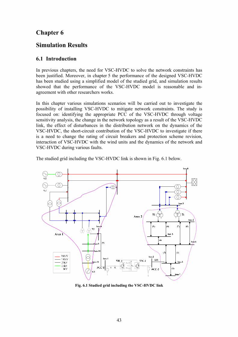
43
Chapter 6 Simulation Results 6.1 Introduction In previous chapters, the need for VSC-HVDC to solve the network constraints has been justified. Moreover, in chapter 5 the performance of the designed VSC-HVDC has been studied using a simplified model of the studied grid, and simulation results showed that the performance of the VSC-HVDC model is reasonable and in-agreement with other researchers works. In this chapter various simulations scenarios will be carried out to investigate the possibility of installing VSC-HVDC to mitigate network constraints. The study is focused on: identifying the appropriate PCC of the VSC-HVDC through voltage sensitivity analysis, the change in the network topology as a result of the VSC-HVDC link, the effect of disturbances in the distribution network on the dynamics of the VSC-HVDC, the short-circuit contribution of the VSC-HVDC to investigate if there is a need to change the rating of circuit breakers and protection scheme revision, interaction of VSC-HVDC with the wind units and the dynamics of the network and VSC-HVDC during various faults. The studied grid including the VSC-HVDC link is shown in Fig. 6.1 below.
dcu2 dcC
2 dcC
Fig. 6.1 Studied grid including the VSC-HVDC link
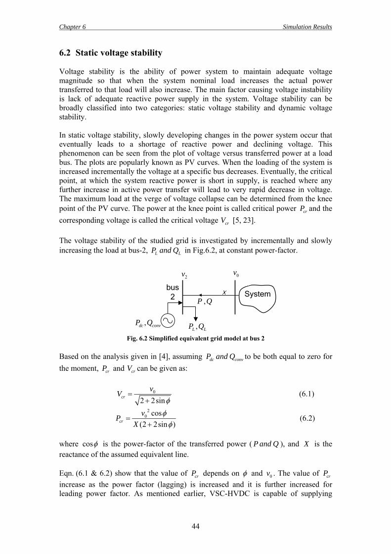
Chapter 6 Simulation Results
44
6.2 Static voltage stability Voltage stability is the ability of power system to maintain adequate voltage magnitude so that when the system nominal load increases the actual power transferred to that load will also increase. The main factor causing voltage instability is lack of adequate reactive power supply in the system. Voltage stability can be broadly classified into two categories: static voltage stability and dynamic voltage stability. In static voltage stability, slowly developing changes in the power system occur that eventually leads to a shortage of reactive power and declining voltage. This phenomenon can be seen from the plot of voltage versus transferred power at a load bus. The plots are popularly known as PV curves. When the loading of the system is increased incrementally the voltage at a specific bus decreases. Eventually, the critical point, at which the system reactive power is short in supply, is reached where any further increase in active power transfer will lead to very rapid decrease in voltage. The maximum load at the verge of voltage collapse can be determined from the knee point of the PV curve. The power at the knee point is called critical power crP and the corresponding voltage is called the critical voltage crV [5, 23]. The voltage stability of the studied grid is investigated by incrementally and slowly increasing the load at bus-2, L LP and Q in Fig.6.2, at constant power-factor.
bus 2
,L LP Q,dc convP Q
System,P Q
0v2v
Fig. 6.2 Simplified equivalent grid model at bus 2
Based on the analysis given in [4], assuming dc convP and Q to be both equal to zero for the moment, crP and crV can be given as:
0
2 2sincrvV
φ=
+ (6.1)
2
0 cos(2 2sin )crvP
Xφφ
=+
(6.2)
where cosφ is the power-factor of the transferred power ( P and Q ), and X is the reactance of the assumed equivalent line. Eqn. (6.1 & 6.2) show that the value of crP depends on φ and 0v . The value of crP increase as the power factor (lagging) is increased and it is further increased for leading power factor. As mentioned earlier, VSC-HVDC is capable of supplying
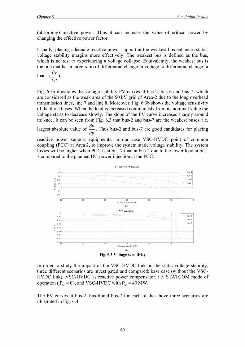
Chapter 6 Simulation Results
45
(absorbing) reactive power. Thus it can increase the value of critical power by changing the effective power factor. Usually, placing adequate reactive power support at the weakest bus enhances static-voltage stability margins more effectively. The weakest bus is defined as the bus, which is nearest to experiencing a voltage collapse. Equivalently, the weakest bus is the one that has a large ratio of differential change in voltage to differential change in
load ( vp∂∂
).
Fig. 6.3a illustrates the voltage stability PV curves at bus-2, bus-6 and bus-7, which are considered as the weak area of the 50 kV grid of Area-2 due to the long overhead transmission lines, line 7 and line 8. Moreover, Fig. 6.3b shows the voltage sensitivity of the three buses. When the load is increased continuously from its nominal value the voltage starts to decrease slowly. The slope of the PV curve increases sharply around its knee. It can be seen from Fig. 6.3 that bus-2 and bus-7 are the weakest buses, i.e.
largest absolute value of vp∂∂
. Thus bus-2 and bus-7 are good candidates for placing
reactive power support equipments, in our case VSC-HVDC point of common coupling (PCC) at Area 2, to improve the system static voltage stability. The system losses will be higher when PCC is at bus-7 than at bus-2 due to the lower load at bus-7 compared to the planned DC-power injection at the PCC.
15 20 25 30 35 40 45-0.08
-0.07
-0.06
-0.05
-0.04
-0.03
-0.02
-0.01
0
P:Load at bus-2 (MW)
∂ v/∂
p
V/P sensitivity
15 20 25 30 35 40 45
0.65
0.7
0.75
0.8
0.85
0.9
0.95
1
P:Load at bus-2 (MW)
Vol
tage
in p
.u.
PV curve for basecase
bus-2
bus-6
bus-7
bus-2
bus-6
bus-7
knee
(a)
(b) Fig. 6.3 Voltage sensitivity
In order to study the impact of the VSC-HVDC link on the static voltage stability, three different scenarios are investigated and compared: base case (without the VSC-HVDC link), VSC-HVDC as reactive power compensator, i.e. STATCOM mode of operation ( 0dcP = ), and VSC-HVDC with 40dcP = MW. The PV curves at bus-2, bus-6 and bus-7 for each of the above three scenarios are illustrated in Fig. 6.4.
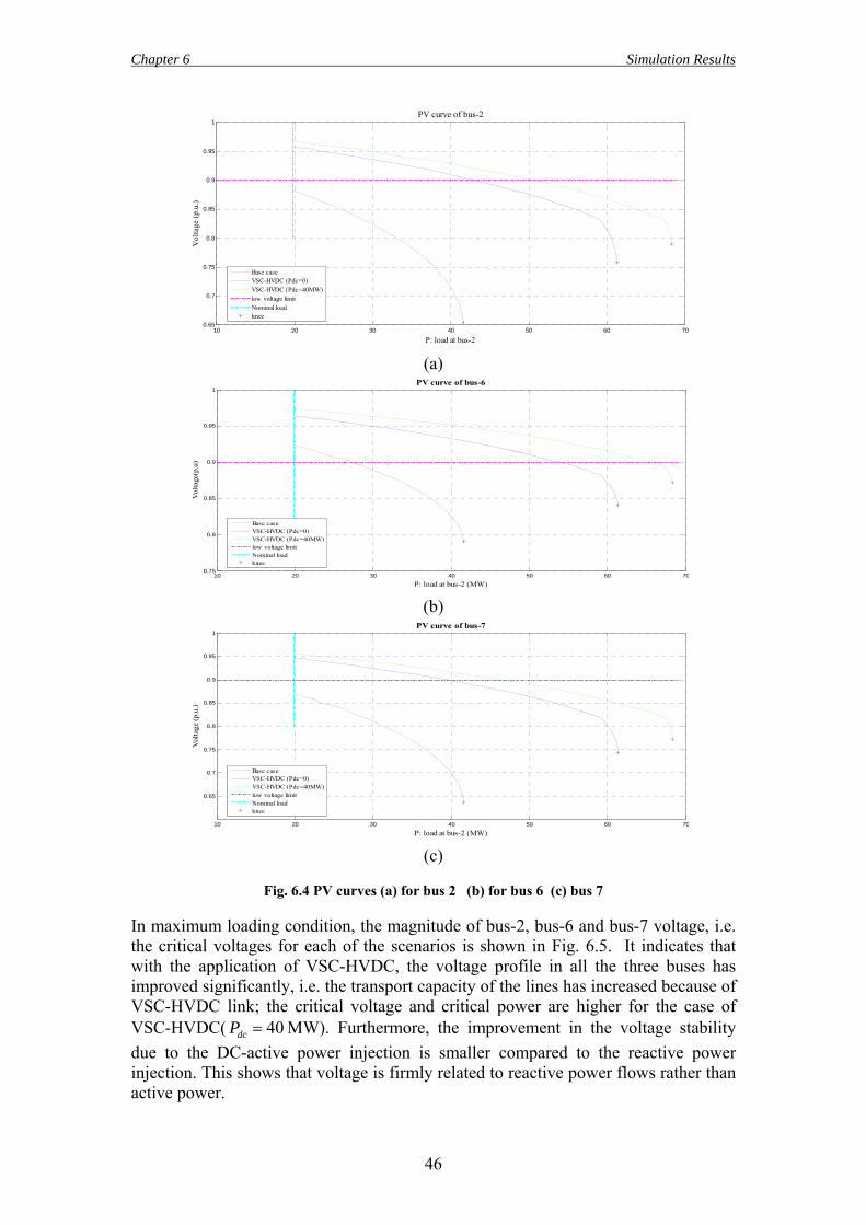
Chapter 6 Simulation Results
46
10 20 30 40 50 60 700.65
0.7
0.75
0.8
0.85
0.9
0.95
1PV curve of bus-2
P: load at bus-2
Vol
tage
(p.u
.)
Base caseVSC-HVDC (Pdc=0)VSC-HVDC (Pdc=40MW)low voltage limitNominal loadknee
(a)
10 20 30 40 50 60 700.75
0.8
0.85
0.9
0.95
1PV curve of bus-6
P: load at bus-2 (MW)
Vol
tage
(p.u
)
Base caseVSC-HVDC (Pdc=0)VSC-HVDC (Pdc=40MW)low voltage limitNominal loadknee
(b)
10 20 30 40 50 60 70
0.65
0.7
0.75
0.8
0.85
0.9
0.95
1PV curve of bus-7
P: load at bus-2 (MW)
Vol
tage
(p.u
.)
Base caseVSC-HVDC (Pdc=0)VSC-HVDC (Pdc=40MW)low voltage limitNominal loadknee
(c)
Fig. 6.4 PV curves (a) for bus 2 (b) for bus 6 (c) bus 7
In maximum loading condition, the magnitude of bus-2, bus-6 and bus-7 voltage, i.e. the critical voltages for each of the scenarios is shown in Fig. 6.5. It indicates that with the application of VSC-HVDC, the voltage profile in all the three buses has improved significantly, i.e. the transport capacity of the lines has increased because of VSC-HVDC link; the critical voltage and critical power are higher for the case of VSC-HVDC( 40dcP = MW). Furthermore, the improvement in the voltage stability due to the DC-active power injection is smaller compared to the reactive power injection. This shows that voltage is firmly related to reactive power flows rather than active power.

Chapter 6 Simulation Results
47
bus-2 bus-6 bus-70
0.1
0.2
0.3
0.4
0.5
0.6
0.7
0.8
0.9
Criti
cal v
olta
ge (p
.u.)
0
10
20
30
40
50
60
70
Criti
cal p
ower
(MW
)
VSC-HVDC(Pdc=40)VSC-HVDC(Pdc=0)Basecase
VSC-HVDC(Pdc=40)VSC-HVDC(Pdc=0)Basecase
(a) (b)
Fig. 6.5 Critical voltage and power
A more direct way to illustrate the voltage support function of the VSC-HVDC could be simulating a step change in the load at bus-2 at constant power factor, see Fig. 6.6. VSC-HVDC stabilizes the voltage at bus-2 as the AC load is continuously changed by adjusting it reactive power support accordingly while keeping the DC-power transport constant with in its capability curve.
1.3001.0200.7400.4600.180-0.100 [s]
50.00
40.00
30.00
20.00
10.00
Load at bus-2: P in MW
1.3001.0200.7400.4600.180-0.100 [s]
0.646
0.492
0.337
0.182
0.027
-0.127
VSC-2: Reactive power in p.u.VSC-1: Reactive power in p.u.
1.3001.0200.7400.4600.180-0.100 [s]
0.980
0.970
0.960
0.950
0.940
0.930
bus-2: Voltage Magnitude in p.u.1.3001.0200.7400.4600.180-0.100 [s]
0.900
0.880
0.860
0.840
0.820
0.800
VSC-2: Active power in p.u.
Fig. 6.6 Dynamic voltage support of VSC-HVDC The above discussions and conclusion are drawn based on static voltage stability analysis of the studied grid at normal operation condition. A thorough investigation of static voltage stability requires N-1 contingency analysis to get the exact PV curve. But still the system will have better static voltage stability when operated with VSC-HVDC ( 40dcP = MW) in each outage case. Thus still the drawn conclusions are valid. 6.3 Effect of VSC- HVDC on rotor angle Rotor angle stability concerns the ability of interconnected synchronous machines in a power system to remain in synchronism under normal operating conditions and after being subjected to a disturbance. The transient rotor stability is influenced by initial
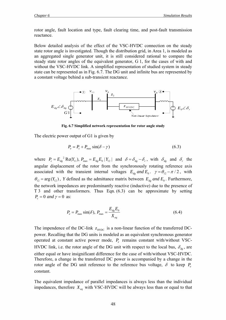
Chapter 6 Simulation Results
48
rotor angle, fault location and type, fault clearing time, and post-fault transmission reactance. Below detailed analysis of the effect of the VSC-HVDC connection on the steady state rotor angle is investigated. Though the distribution grid, in Area 1, is modeled as an aggregated single generator unit, it is still considered rational to compare the steady state rotor angles of the equivalent generator, G 1, for the cases of with and without the VSC-HVDC link. A simplified representation of studied system in steady state can be represented as in Fig. 6.7. The DG unit and infinite bus are represented by a constant voltage behind a sub-transient reactance.
H V D Cz
2z
1G
0v8v
1z
1 1v
0 rE δ∠dg dgE δ∠
Fig. 6.7 Simplified network representation for rotor angle study The electric power output of G1 is given by max sin( )e cP P P δ γ= + − (6.3) where 2
11 max 0 12Re( ), | |c dg dgP E Y P E E Y= = and dg rδ δ δ= − , with dgδ and rδ the angular displacement of the rotor from the synchronously rotating reference axis associated with the transient internal voltages 0dgE and E . 12 / 2γ θ π= − , with
12 12arg ( )Yθ = , Y defined as the admittance matrix between 0dgE and E . Furthermore, the network impedances are predominantly reactive (inductive) due to the presence of T 3 and other transformers. Thus Eqn. (6.3) can be approximate by setting
0 0cP and γ= = as:
0max maxsin( ), dg
eeq
E EP P P
Xδ= = (6.4)
The impendence of the DC-link HVDCz is a non-linear function of the transferred DC-power. Recalling that the DG units is modeled as an equivalent synchronous generator operated at constant active power mode, eP remains constant with/without VSC-HVDC link, i.e. the rotor angle of the DG unit with respect to the local bus, dgδ , are either equal or have insignificant difference for the case of with/without VSC-HVDC. Therefore, a change in the transferred DC power is accompanied by a change in the rotor angle of the DG unit reference to the reference bus voltage, δ to keep eP constant. The equivalent impedance of parallel impedances is always less than the individual impedances, therefore eqX with VSC-HVDC will be always less than or equal to that
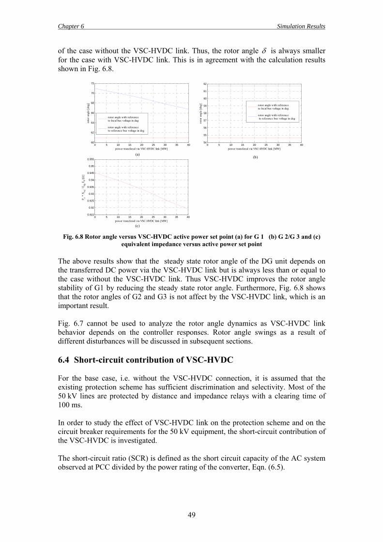
Chapter 6 Simulation Results
49
of the case without the VSC-HVDC link. Thus, the rotor angle δ is always smaller for the case with VSC-HVDC link. This is in agreement with the calculation results shown in Fig. 6.8.
0 5 10 15 20 25 30 35 4060
62
64
66
68
70
72
power transfered via VSC-HVDC link [MW]
roto
r ang
le [d
eg]
rotor angle with referenceto local bus voltage in deg
rotor angle with referenceto reference bus voltage in deg
0 5 10 15 20 25 30 35 4054
55
56
57
58
59
60
61
62
power transfered via VSC-HVDC link [MW]
roto
r ang
le [d
eg] rotor angle with reference
to local bus voltage in deg
rotor angle with reference to reference bus voltage in deg
0 5 10 15 20 25 30 35 400.915
0.92
0.925
0.93
0.935
0.94
0.945
0.95
0.955
P e * X
eq /
E dg E
0 [ Ω]
power transfered via VSC-HVDC link [MW]
(a)(b)
(c)
Fig. 6.8 Rotor angle versus VSC-HVDC active power set point (a) for G 1 (b) G 2/G 3 and (c) equivalent impedance versus active power set point
The above results show that the steady state rotor angle of the DG unit depends on the transferred DC power via the VSC-HVDC link but is always less than or equal to the case without the VSC-HVDC link. Thus VSC-HVDC improves the rotor angle stability of G1 by reducing the steady state rotor angle. Furthermore, Fig. 6.8 shows that the rotor angles of G2 and G3 is not affect by the VSC-HVDC link, which is an important result. Fig. 6.7 cannot be used to analyze the rotor angle dynamics as VSC-HVDC link behavior depends on the controller responses. Rotor angle swings as a result of different disturbances will be discussed in subsequent sections. 6.4 Short-circuit contribution of VSC-HVDC For the base case, i.e. without the VSC-HVDC connection, it is assumed that the existing protection scheme has sufficient discrimination and selectivity. Most of the 50 kV lines are protected by distance and impedance relays with a clearing time of 100 ms. In order to study the effect of VSC-HVDC link on the protection scheme and on the circuit breaker requirements for the 50 kV equipment, the short-circuit contribution of the VSC-HVDC is investigated. The short-circuit ratio (SCR) is defined as the short circuit capacity of the AC system observed at PCC divided by the power rating of the converter, Eqn. (6.5).
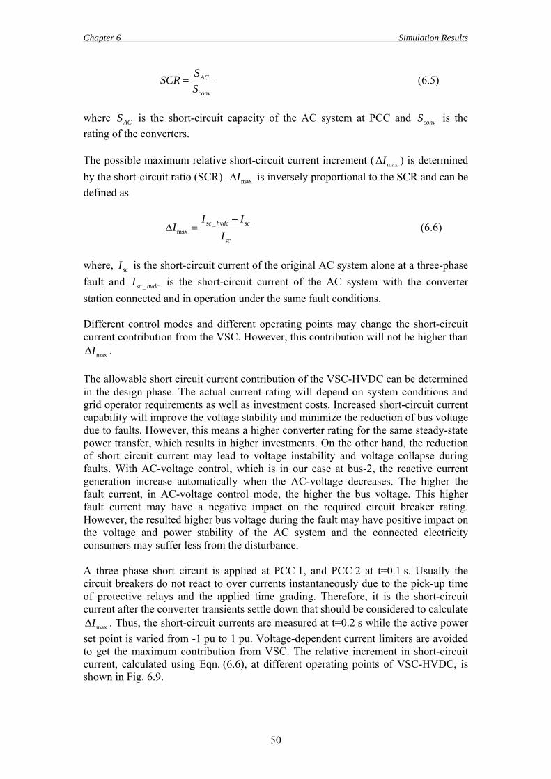
Chapter 6 Simulation Results
50
AC
conv
SSCRS
= (6.5)
where ACS is the short-circuit capacity of the AC system at PCC and convS is the rating of the converters. The possible maximum relative short-circuit current increment ( maxIΔ ) is determined by the short-circuit ratio (SCR). maxIΔ is inversely proportional to the SCR and can be defined as
_max
sc hvdc sc
sc
I II
I−
Δ = (6.6)
where, scI is the short-circuit current of the original AC system alone at a three-phase fault and _sc hvdcI is the short-circuit current of the AC system with the converter station connected and in operation under the same fault conditions. Different control modes and different operating points may change the short-circuit current contribution from the VSC. However, this contribution will not be higher than
maxIΔ . The allowable short circuit current contribution of the VSC-HVDC can be determined in the design phase. The actual current rating will depend on system conditions and grid operator requirements as well as investment costs. Increased short-circuit current capability will improve the voltage stability and minimize the reduction of bus voltage due to faults. However, this means a higher converter rating for the same steady-state power transfer, which results in higher investments. On the other hand, the reduction of short circuit current may lead to voltage instability and voltage collapse during faults. With AC-voltage control, which is in our case at bus-2, the reactive current generation increase automatically when the AC-voltage decreases. The higher the fault current, in AC-voltage control mode, the higher the bus voltage. This higher fault current may have a negative impact on the required circuit breaker rating. However, the resulted higher bus voltage during the fault may have positive impact on the voltage and power stability of the AC system and the connected electricity consumers may suffer less from the disturbance. A three phase short circuit is applied at PCC 1, and PCC 2 at t=0.1 s. Usually the circuit breakers do not react to over currents instantaneously due to the pick-up time of protective relays and the applied time grading. Therefore, it is the short-circuit current after the converter transients settle down that should be considered to calculate
maxIΔ . Thus, the short-circuit currents are measured at t=0.2 s while the active power set point is varied from -1 pu to 1 pu. Voltage-dependent current limiters are avoided to get the maximum contribution from VSC. The relative increment in short-circuit current, calculated using Eqn. (6.6), at different operating points of VSC-HVDC, is shown in Fig. 6.9.
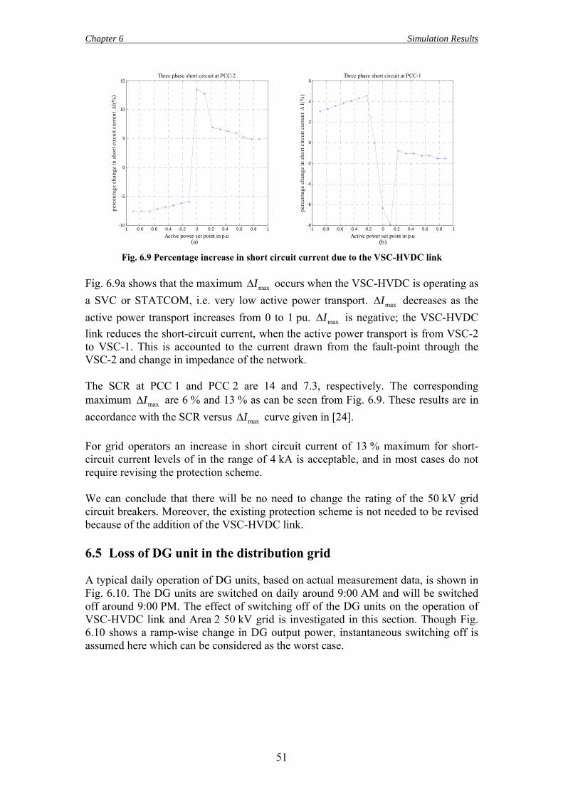
Chapter 6 Simulation Results
51
-1 -0.8 -0.6 -0.4 -0.2 0 0.2 0.4 0.6 0.8 1-10
-5
0
5
10
15Three phase short circuit at PCC-2
perc
enta
ge c
hang
e in
shor
t cir
cuit
curr
ent
Δ I(%
)
Active power set point in p.u-1 -0.8 -0.6 -0.4 -0.2 0 0.2 0.4 0.6 0.8 1
-8
-6
-4
-2
0
2
4
6Three phase short circuit at PCC-1
perc
enta
ge c
hang
e in
shor
t circ
uit c
urre
nt
Δ I(
%)
Active power set point in p.u(a) (b)
Fig. 6.9 Percentage increase in short circuit current due to the VSC-HVDC link
Fig. 6.9a shows that the maximum maxIΔ occurs when the VSC-HVDC is operating as a SVC or STATCOM, i.e. very low active power transport. maxIΔ decreases as the active power transport increases from 0 to 1 pu. maxIΔ is negative; the VSC-HVDC link reduces the short-circuit current, when the active power transport is from VSC-2 to VSC-1. This is accounted to the current drawn from the fault-point through the VSC-2 and change in impedance of the network. The SCR at PCC 1 and PCC 2 are 14 and 7.3, respectively. The corresponding maximum maxIΔ are 6 % and 13 % as can be seen from Fig. 6.9. These results are in accordance with the SCR versus maxIΔ curve given in [24]. For grid operators an increase in short circuit current of 13 % maximum for short-circuit current levels of in the range of 4 kA is acceptable, and in most cases do not require revising the protection scheme. We can conclude that there will be no need to change the rating of the 50 kV grid circuit breakers. Moreover, the existing protection scheme is not needed to be revised because of the addition of the VSC-HVDC link. 6.5 Loss of DG unit in the distribution grid A typical daily operation of DG units, based on actual measurement data, is shown in Fig. 6.10. The DG units are switched on daily around 9:00 AM and will be switched off around 9:00 PM. The effect of switching off of the DG units on the operation of VSC-HVDC link and Area 2 50 kV grid is investigated in this section. Though Fig. 6.10 shows a ramp-wise change in DG output power, instantaneous switching off is assumed here which can be considered as the worst case.
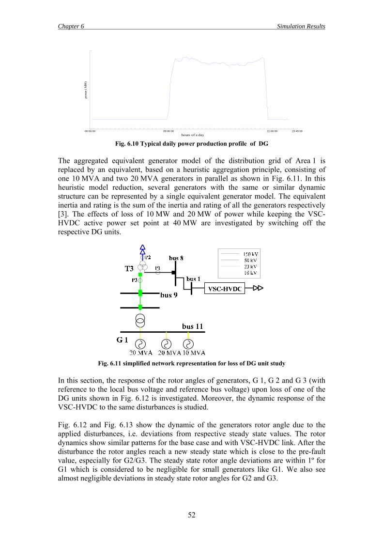
Chapter 6 Simulation Results
52
00:00:00 09:00:00 21:00:00 23:45:00
hours of a day
pow
er (
MW
)
Fig. 6.10 Typical daily power production profile of DG
The aggregated equivalent generator model of the distribution grid of Area 1 is replaced by an equivalent, based on a heuristic aggregation principle, consisting of one 10 MVA and two 20 MVA generators in parallel as shown in Fig. 6.11. In this heuristic model reduction, several generators with the same or similar dynamic structure can be represented by a single equivalent generator model. The equivalent inertia and rating is the sum of the inertia and rating of all the generators respectively [3]. The effects of loss of 10 MW and 20 MW of power while keeping the VSC-HVDC active power set point at 40 MW are investigated by switching off the respective DG units.
Fig. 6.11 simplified network representation for loss of DG unit study
In this section, the response of the rotor angles of generators, G 1, G 2 and G 3 (with reference to the local bus voltage and reference bus voltage) upon loss of one of the DG units shown in Fig. 6.12 is investigated. Moreover, the dynamic response of the VSC-HVDC to the same disturbances is studied. Fig. 6.12 and Fig. 6.13 show the dynamic of the generators rotor angle due to the applied disturbances, i.e. deviations from respective steady state values. The rotor dynamics show similar patterns for the base case and with VSC-HVDC link. After the disturbance the rotor angles reach a new steady state which is close to the pre-fault value, especially for G2/G3. The steady state rotor angle deviations are within 1º for G1 which is considered to be negligible for small generators like G1. We also see almost negligible deviations in steady state rotor angles for G2 and G3.
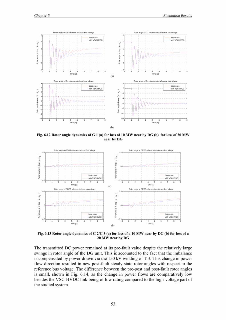
Chapter 6 Simulation Results
53
0 1 2 3 4 5 6 7 8 9-2
-1
0
1
2
3Rotor angle of G1 reference to Local Bus voltage
time [s]
Rot
or a
ngle
in d
eg ( δ
- δ 0 )
0 1 2 3 4 5 6 7 8 9-8
-6
-4
-2
0
2Rotor angle of G1 reference to reference bus voltage
time [s]
Rot
or a
ngle
in d
eg ( δ
- δ 0 )
0 1 2 3 4 5 6 7 8 9-4
-3
-2
-1
0
1
2
3
4Rotor angle of G1 reference to local bus voltage
time [s]
Rot
or a
ngle
in d
eg ( δ
- δ 0 )
0 1 2 3 4 5 6 7 8 9-12
-10
-8
-6
-4
-2
0
2Rotor angle of G1 reference to reference bus voltage
time [s]
Rot
or a
ngle
in d
eg ( δ
- δ 0 )
base casewith VSC-HVDC
base casewith VSC-HVDC
base casewith VSC-HVDC
base casewith VSC-HVDC
(a)
(b)
Fig. 6.12 Rotor angle dynamics of G 1 (a) for loss of 10 MW near by DG (b) for loss of 20 MW near by DG
0 1 2 3 4 5 6 7 8 9-0.5
0
0.5Rotor angle of G2/G3 reference to Local Bus voltage
time [s]
Rot
or a
ngle
in d
eg ( δ
- δ 0 )
0 1 2 3 4 5 6 7 8 9-0.5
0
0.5Rotor angle of G2/G3 reference to reference bus voltage
time [s]
Rot
or a
ngle
in d
eg ( δ
- δ 0 )
0 1 2 3 4 5 6 7 8 9-0.5
0
0.5Rotor angle of G2/G3 reference to local bus voltage
time [s]
Rot
or a
ngle
in d
eg ( δ
- δ 0 )
0 1 2 3 4 5 6 7 8 9-0.5
0
0.5Rotor angle of G2/G3 reference to reference bus voltage
time [s]
Rot
or a
ngle
in d
eg ( δ
- δ 0 )
base casewith VSC-HVDC
base casewith VSC-HVDC
base casewith VSC-HVDC
base casewith VSC-HVDC
(a)
(b)
Fig. 6.13 Rotor angle dynamics of G 2/G 3 (a) for loss of a 10 MW near by DG (b) for loss of a 20 MW near by DG
The transmitted DC power remained at its pre-fault value despite the relatively large swings in rotor angle of the DG unit. This is accounted to the fact that the imbalance is compensated by power drawn via the 150 kV winding of T 3. This change in power flow direction resulted in new post-fault steady state rotor angles with respect to the reference bus voltage. The difference between the pre-post and post-fault rotor angles is small, shown in Fig. 6.14, as the change in power flows are comparatively low besides the VSC-HVDC link being of low rating compared to the high-voltage part of the studied system.
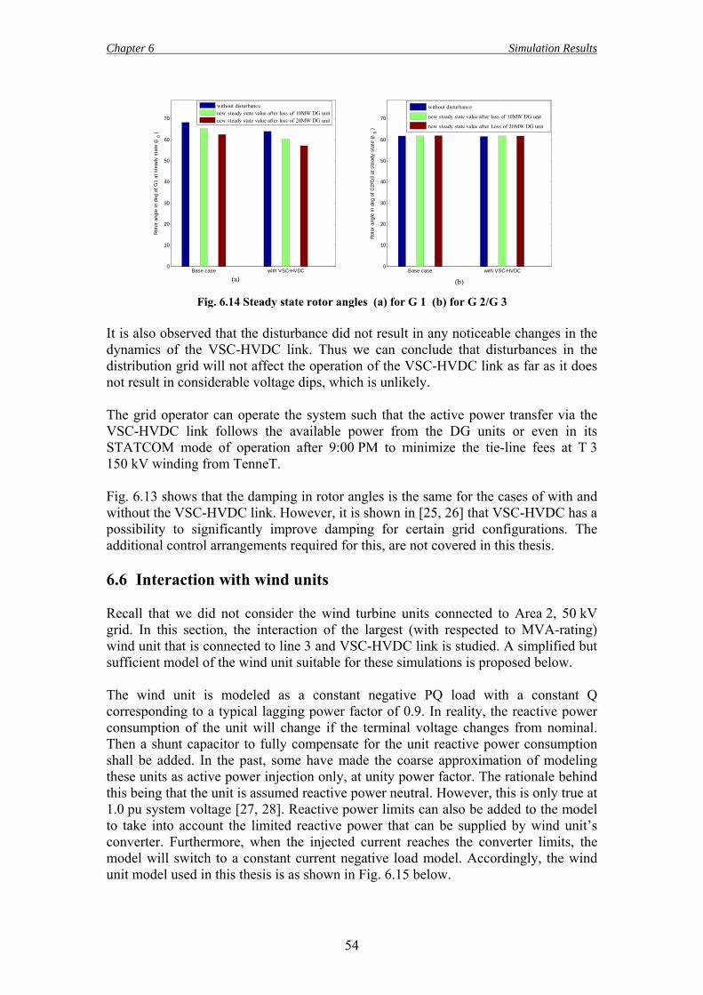
Chapter 6 Simulation Results
54
It is also observed that the disturbance did not result in any noticeable changes in the dynamics of the VSC-HVDC link. Thus we can conclude that disturbances in the distribution grid will not affect the operation of the VSC-HVDC link as far as it does not result in considerable voltage dips, which is unlikely. The grid operator can operate the system such that the active power transfer via the VSC-HVDC link follows the available power from the DG units or even in its STATCOM mode of operation after 9:00 PM to minimize the tie-line fees at T 3 150 kV winding from TenneT. Fig. 6.13 shows that the damping in rotor angles is the same for the cases of with and without the VSC-HVDC link. However, it is shown in [25, 26] that VSC-HVDC has a possibility to significantly improve damping for certain grid configurations. The additional control arrangements required for this, are not covered in this thesis. 6.6 Interaction with wind units Recall that we did not consider the wind turbine units connected to Area 2, 50 kV grid. In this section, the interaction of the largest (with respected to MVA-rating) wind unit that is connected to line 3 and VSC-HVDC link is studied. A simplified but sufficient model of the wind unit suitable for these simulations is proposed below. The wind unit is modeled as a constant negative PQ load with a constant Q corresponding to a typical lagging power factor of 0.9. In reality, the reactive power consumption of the unit will change if the terminal voltage changes from nominal. Then a shunt capacitor to fully compensate for the unit reactive power consumption shall be added. In the past, some have made the coarse approximation of modeling these units as active power injection only, at unity power factor. The rationale behind this being that the unit is assumed reactive power neutral. However, this is only true at 1.0 pu system voltage [27, 28]. Reactive power limits can also be added to the model to take into account the limited reactive power that can be supplied by wind unit’s converter. Furthermore, when the injected current reaches the converter limits, the model will switch to a constant current negative load model. Accordingly, the wind unit model used in this thesis is as shown in Fig. 6.15 below.
Base case with VSC-HVDC0
10
20
30
40
50
60
70
Rot
or a
ngle
in d
eg o
f G1
at s
tead
y st
ate
( δ 0 )
Base case with VSC-HVDC0
10
20
30
40
50
60
70
Rot
or a
ngle
in d
eg o
f G2/
G3
at s
tead
y st
ate
( δ 0 )
without disturbancenew steady state value after loss of 10MW DG unitnew steady state value after loss of 20MW DG unit
without disturbance
new steady state value after loss of 10MW DG unit
new steady state value after Loss of 20MW DG unit
(a) (b)
Fig. 6.14 Steady state rotor angles (a) for G 1 (b) for G 2/G 3
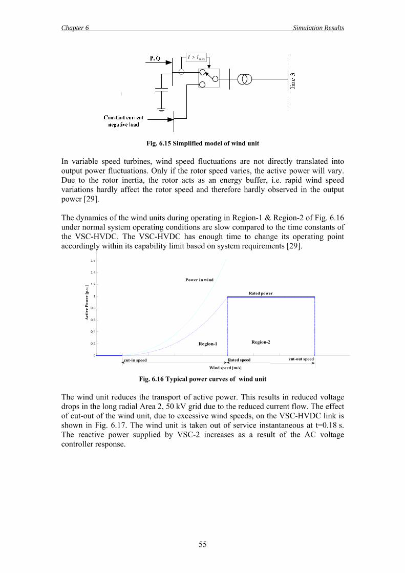
Chapter 6 Simulation Results
55
m axI I>
Fig. 6.15 Simplified model of wind unit In variable speed turbines, wind speed fluctuations are not directly translated into output power fluctuations. Only if the rotor speed varies, the active power will vary. Due to the rotor inertia, the rotor acts as an energy buffer, i.e. rapid wind speed variations hardly affect the rotor speed and therefore hardly observed in the output power [29]. The dynamics of the wind units during operating in Region-1 & Region-2 of Fig. 6.16 under normal system operating conditions are slow compared to the time constants of the VSC-HVDC. The VSC-HVDC has enough time to change its operating point accordingly within its capability limit based on system requirements [29].
0
0.2
0.4
0.6
0.8
1
1.2
1.4
1.6
Act
ive
Pow
er [p
.u.]
Wind speed [m/s]
Power in wind
Rated power
Rated speed cut-out speedcut-in speed
Region-1 Region-2
Fig. 6.16 Typical power curves of wind unit The wind unit reduces the transport of active power. This results in reduced voltage drops in the long radial Area 2, 50 kV grid due to the reduced current flow. The effect of cut-out of the wind unit, due to excessive wind speeds, on the VSC-HVDC link is shown in Fig. 6.17. The wind unit is taken out of service instantaneous at t=0.18 s. The reactive power supplied by VSC-2 increases as a result of the AC voltage controller response.
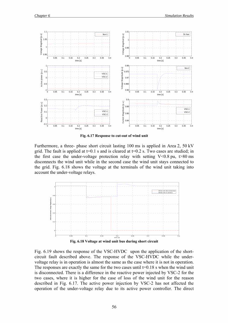
Chapter 6 Simulation Results
56
0 0.05 0.1 0.15 0.2 0.25 0.3 0.35 0.40.95
1
1.05
1.1
Vol
tage
Mag
nitu
d [p
.u]
time [s]0 0.05 0.1 0.15 0.2 0.25 0.3 0.35 0.4
0.98
0.99
1
1.01
Vol
tage
Mag
nitu
d [p
.u]
time [s]
0 0.05 0.1 0.15 0.2 0.25 0.3 0.35 0.4-1
-0.5
0
0.5
1
Act
ive
pow
er [p
.u.]
time [s]0 0.05 0.1 0.15 0.2 0.25 0.3 0.35 0.4
0.96
0.965
0.97
0.975
0.98
Vol
tage
Mag
nitu
de [p
.u]
time [s]
0 0.05 0.1 0.15 0.2 0.25 0.3 0.35 0.4-0.1
0
0.1
0.2
0.3
Rea
ctiv
e P
ower
[p.u
.]
time [s]0 0.05 0.1 0.15 0.2 0.25 0.3 0.35 0.4
0.84
0.86
0.88
0.9
Cur
rent
Mag
nitu
de [p
.u.]
time [s]
bus-1 Dc bus
VSC-1VSC-2
bus-2
VSC-1VSC-2
VSC-1VSC-2
Fig. 6.17 Response to cut-out of wind unit Furthermore, a three- phase short circuit lasting 100 ms is applied in Area 2, 50 kV grid. The fault is applied at t=0.1 s and is cleared at t=0.2 s. Two cases are studied; in the first case the under-voltage protection relay with setting V<0.8 pu, t>80 ms disconnects the wind unit while in the second case the wind unit stays connected to the grid. Fig. 6.18 shows the voltage at the terminals of the wind unit taking into account the under-voltage relays.
0 0.05 0.1 0.15 0.2 0.25 0.3 0.35 0.4
0
0.2
0.4
0.6
0.8
1
Win
d un
it te
rmin
al: V
olta
ge M
agni
tud
[p.u
]
time [s]
Wind unit disconnectedWind unit in service
Fig. 6.18 Voltage at wind unit bus during short circuit
Fig. 6.19 shows the response of the VSC-HVDC upon the application of the short- circuit fault described above. The response of the VSC-HVDC while the under-voltage relay is in operation is almost the same as the case where it is not in operation. The responses are exactly the same for the two cases until t=0.18 s when the wind unit is disconnected. There is a difference in the reactive power injected by VSC-2 for the two cases, where it is higher for the case of loss of the wind unit for the reason described in Fig. 6.17. The active power injection by VSC-2 has not affected the operation of the under-voltage relay due to its active power controller. The direct
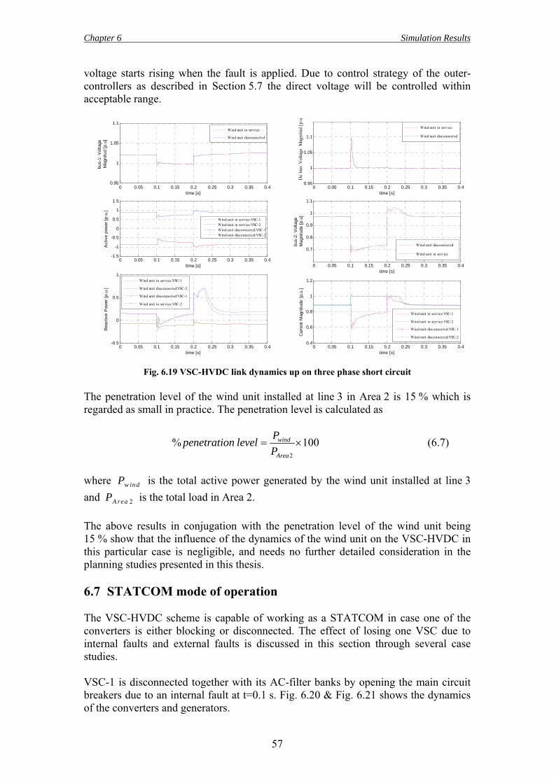
Chapter 6 Simulation Results
57
voltage starts rising when the fault is applied. Due to control strategy of the outer-controllers as described in Section 5.7 the direct voltage will be controlled within acceptable range.
0 0.05 0.1 0.15 0.2 0.25 0.3 0.35 0.40.95
1
1.05
1.1
bus-
1: V
olta
ge
Mag
nitu
d [p
.u]
time [s]0 0.05 0.1 0.15 0.2 0.25 0.3 0.35 0.4
0.95
1
1.05
1.1
Dc
bus:
Vol
tage
Mag
nitu
d [p
.u]
time [s]
0 0.05 0.1 0.15 0.2 0.25 0.3 0.35 0.4-1.5
-1
-0.5
0
0.5
1
1.5
Act
ive
pow
er [p
.u.]
time [s] 0 0.05 0.1 0.15 0.2 0.25 0.3 0.35 0.4
0.7
0.8
0.9
1
1.1
bus-
2: V
olta
ge M
agni
tude
[p.u
]
time [s]
0 0.05 0.1 0.15 0.2 0.25 0.3 0.35 0.4-0.5
0
0.5
1
Rea
ctiv
e P
ower
[p.u
.]
time [s]0 0.05 0.1 0.15 0.2 0.25 0.3 0.35 0.4
0.4
0.6
0.8
1
1.2
Cur
rent
Mag
nitu
de [p
.u.]
time [s]
Wind unit in service
Wind unit disconnected
Wind unit in service
Wind unit disconnected
Wind unit in service:VSC-1Wind unit in service:VSC-2Wind unit disconnected:VSC-1Wind unit disconnected:VSC-2
Wind unit disconnected
Wind unit in service
Wind unit in service:VSC-1
Wind unit disconnected:VSC-2
Wind unit disconnected:VSC-1
Wind unit in service:VSC-2
Wind unit in service:VSC-1
Wind unit in service:VSC-2
Wind unit disconnected:VSC-1
Wind unit disconnected:VSC-2
Fig. 6.19 VSC-HVDC link dynamics up on three phase short circuit The penetration level of the wind unit installed at line 3 in Area 2 is 15 % which is regarded as small in practice. The penetration level is calculated as
2
% 100wind
Area
Ppenetration levelP
= × (6.7)
where w in dP is the total active power generated by the wind unit installed at line 3 and 2A reaP is the total load in Area 2. The above results in conjugation with the penetration level of the wind unit being 15 % show that the influence of the dynamics of the wind unit on the VSC-HVDC in this particular case is negligible, and needs no further detailed consideration in the planning studies presented in this thesis. 6.7 STATCOM mode of operation The VSC-HVDC scheme is capable of working as a STATCOM in case one of the converters is either blocking or disconnected. The effect of losing one VSC due to internal faults and external faults is discussed in this section through several case studies. VSC-1 is disconnected together with its AC-filter banks by opening the main circuit breakers due to an internal fault at t=0.1 s. Fig. 6.20 & Fig. 6.21 shows the dynamics of the converters and generators.
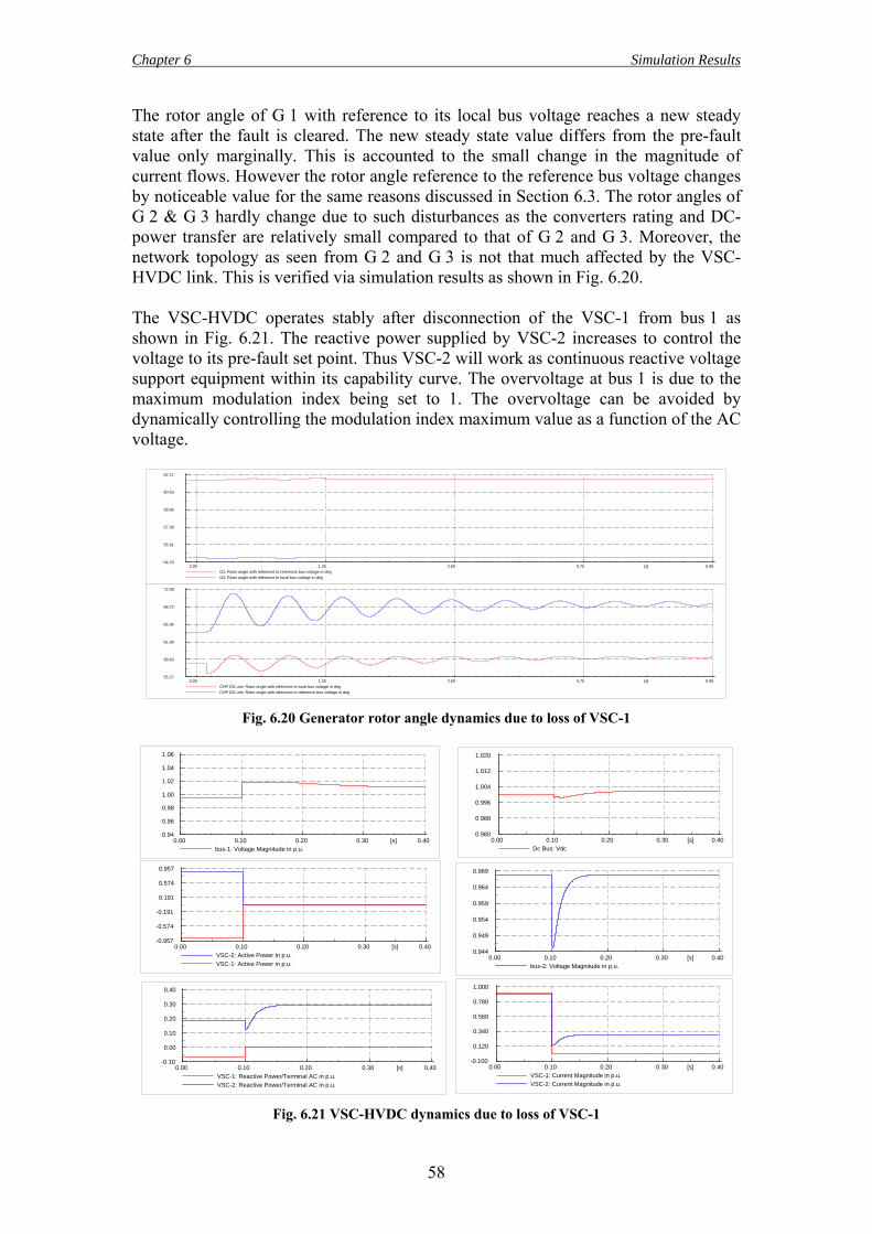
Chapter 6 Simulation Results
58
The rotor angle of G 1 with reference to its local bus voltage reaches a new steady state after the fault is cleared. The new steady state value differs from the pre-fault value only marginally. This is accounted to the small change in the magnitude of current flows. However the rotor angle reference to the reference bus voltage changes by noticeable value for the same reasons discussed in Section 6.3. The rotor angles of G 2 & G 3 hardly change due to such disturbances as the converters rating and DC-power transfer are relatively small compared to that of G 2 and G 3. Moreover, the network topology as seen from G 2 and G 3 is not that much affected by the VSC-HVDC link. This is verified via simulation results as shown in Fig. 6.20. The VSC-HVDC operates stably after disconnection of the VSC-1 from bus 1 as shown in Fig. 6.21. The reactive power supplied by VSC-2 increases to control the voltage to its pre-fault set point. Thus VSC-2 will work as continuous reactive voltage support equipment within its capability curve. The overvoltage at bus 1 is due to the maximum modulation index being set to 1. The overvoltage can be avoided by dynamically controlling the modulation index maximum value as a function of the AC voltage.
5.003.752.501.250.00 [s]
62.11
60.53
58.96
57.38
55.81
54.23
G2: Rotor angle with reference to reference bus voltage in degG2: Rotor angle with reference to local bus voltage in deg
5.003.752.501.250.00 [s]
72.08
68.72
65.36
61.99
58.63
55.27
CHP DG unit: Rotor angle with reference to local bus voltage in degCHP DG unit: Rotor angle with reference to reference bus voltage in deg
Fig. 6.20 Generator rotor angle dynamics due to loss of VSC-1
0.400.300.200.100.00 [s]
1.06
1.04
1.02
1.00
0.98
0.96
0.94
bus-1: Voltage Magnitude in p.u.
0.400.300.200.100.00 [s]
0.957
0.574
0.191
-0.191
-0.574
-0.957
VSC-2: Active Power in p.u.VSC-1: Active Power in p.u.
0.400.300.200.100.00 [s]
1.020
1.012
1.004
0.996
0.988
0.980
Dc Bus: Vdc
0.400.300.200.100.00 [s]
1.000
0.780
0.560
0.340
0.120
-0.100
VSC-1: Current Magnitude in p.u.VSC-2: Current Magnitude in p.u.
0.400.300.200.100.00 [s]
0.40
0.30
0.20
0.10
0.00
-0.10
VSC-1: Reactive Power/Terminal AC in p.u.VSC-2: Reactive Power/Terminal AC in p.u.
0.400.300.200.100.00 [s]
0.969
0.964
0.959
0.954
0.949
0.944
bus-2: Voltage Magnitude in p.u.
Fig. 6.21 VSC-HVDC dynamics due to loss of VSC-1
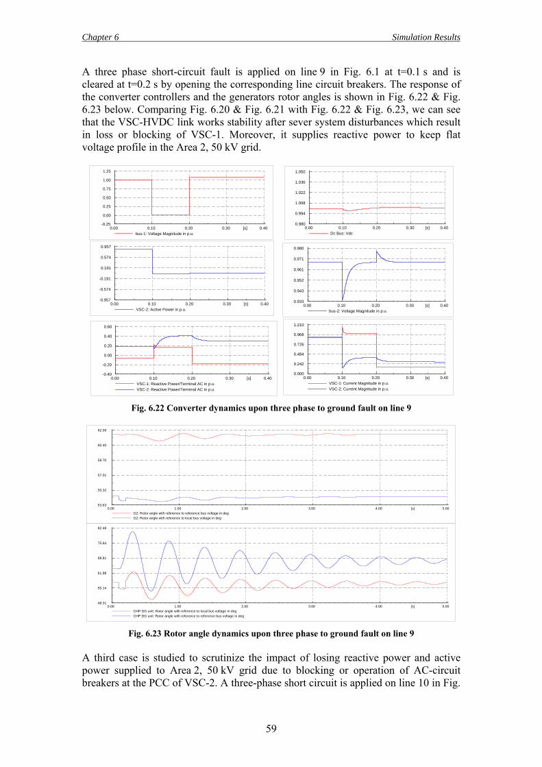
Chapter 6 Simulation Results
59
A three phase short-circuit fault is applied on line 9 in Fig. 6.1 at t=0.1 s and is cleared at t=0.2 s by opening the corresponding line circuit breakers. The response of the converter controllers and the generators rotor angles is shown in Fig. 6.22 & Fig. 6.23 below. Comparing Fig. 6.20 & Fig. 6.21 with Fig. 6.22 & Fig. 6.23, we can see that the VSC-HVDC link works stability after sever system disturbances which result in loss or blocking of VSC-1. Moreover, it supplies reactive power to keep flat voltage profile in the Area 2, 50 kV grid.
0.400.300.200.100.00 [s]
1.050
1.036
1.022
1.008
0.994
0.980
Dc Bus: Vdc
0.400.300.200.100.00 [s]
0.957
0.574
0.191
-0.191
-0.574
-0.957
VSC-2: Active Power in p.u.
0.400.300.200.100.00 [s]
1.25
1.00
0.75
0.50
0.25
0.00
-0.25
bus-1: Voltage Magnitude in p.u.
0.400.300.200.100.00 [s]
1.210
0.968
0.726
0.484
0.242
0.000
VSC-1: Current Magnitude in p.u.VSC-2: Current Magnitude in p.u.
0.400.300.200.100.00 [s]
0.60
0.40
0.20
0.00
-0.20
-0.40
VSC-1: Reactive Power/Terminal AC in p.u.VSC-2: Reactive Power/Terminal AC in p.u.
0.400.300.200.100.00 [s]
0.980
0.971
0.961
0.952
0.943
0.933
bus-2: Voltage Magnitude in p.u.
Fig. 6.22 Converter dynamics upon three phase to ground fault on line 9
5.004.003.002.001.000.00 [s]
62.09
60.40
58.70
57.01
55.32
53.63
G2: Rotor angle with reference to reference bus voltage in degG2: Rotor angle with reference to local bus voltage in deg
5.004.003.002.001.000.00 [s]
82.48
75.64
68.81
61.98
55.14
48.31
CHP DG unit: Rotor angle with reference to local bus voltage in degCHP DG unit: Rotor angle with reference to reference bus voltage in deg
Fig. 6.23 Rotor angle dynamics upon three phase to ground fault on line 9 A third case is studied to scrutinize the impact of losing reactive power and active power supplied to Area 2, 50 kV grid due to blocking or operation of AC-circuit breakers at the PCC of VSC-2. A three-phase short circuit is applied on line 10 in Fig.
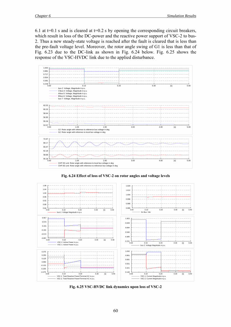
Chapter 6 Simulation Results
60
6.1 at t=0.1 s and is cleared at t=0.2 s by opening the corresponding circuit breakers, which result in loss of the DC-power and the reactive power support of VSC-2 to bus-2. Thus a new steady-state voltage is reached after the fault is cleared that is less than the pre-fault voltage level. Moreover, the rotor angle swing of G1 is less than that of Fig. 6.23 due to the DC-link as shown in Fig. 6.24 below. Fig. 6.25 shows the response of the VSC-HVDC link due to the applied disturbance.
0.400.300.200.100.00 [s]
1.044
0.881
0.717
0.554
0.391
0.228
bus-2: Voltage, Magnitude in p.u.C\bus-4: Voltage, Magnitude in p.u.A\bus-5: Voltage, Magnitude in p.u.B\bus-6: Voltage, Magnitude in p.u.bus-7: Voltage, Magnitude in p.u.
5.004.003.002.001.000.00 [s]
62.02
60.33
58.64
56.95
55.26
53.57
G2: Rotor angle with reference to reference bus voltage in degG2: Rotor angle with reference to local bus voltage in deg
5.004.003.002.001.000.00 [s]
72.67
69.17
65.67
62.18
58.68
55.18
CHP DG unit: Rotor angle with reference to local bus voltage in degCHP DG unit: Rotor angle with reference to reference bus voltage in deg
Fig. 6.24 Effect of loss of VSC-2 on rotor angles and voltage levels
0.400.300.200.100.00 [s]
1.08
1.04
1.00
0.96
0.92
0.88
0.84
bus-1: Voltage Magnitude in p.u.
0.400.300.200.100.00 [s]
0.957
0.574
0.191
-0.191
-0.574
-0.957
VSC-2: Active Power in p.u.VSC-1: Active Power in p.u.
0.400.300.200.100.00 [s]
1.020
1.012
1.004
0.996
0.988
0.980
Dc Bus: Vdc
0.400.300.200.100.00 [s]
1.042
0.861
0.681
0.501
0.321
0.140
VSC-1: Current Magnitude in p.u.VSC-2: Current Magnitude in p.u.
0.400.300.200.100.00 [s]
0.375
0.250
0.125
0.000
-0.125
-0.250
-0.375
VSC-1: Total Reactive Power/Terminal AC in p.u.VSC-2: Total Reactive Power/Terminal AC in p.u.
0.400.300.200.100.00 [s]
1.003
0.849
0.694
0.540
0.385
0.231
bus-2: Voltage Magnitude in p.u.
Fig. 6.25 VSC-HVDC link dynamics upon loss of VSC-2
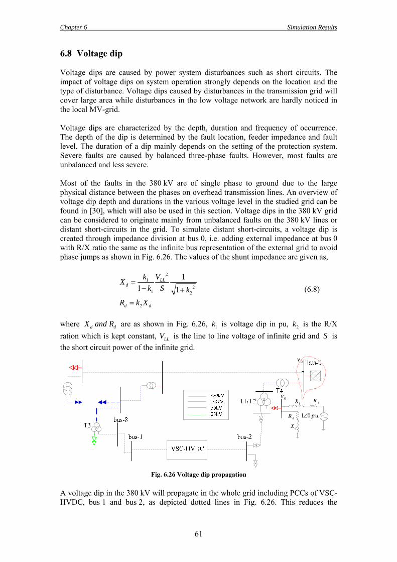
Chapter 6 Simulation Results
61
6.8 Voltage dip Voltage dips are caused by power system disturbances such as short circuits. The impact of voltage dips on system operation strongly depends on the location and the type of disturbance. Voltage dips caused by disturbances in the transmission grid will cover large area while disturbances in the low voltage network are hardly noticed in the local MV-grid. Voltage dips are characterized by the depth, duration and frequency of occurrence. The depth of the dip is determined by the fault location, feeder impedance and fault level. The duration of a dip mainly depends on the setting of the protection system. Severe faults are caused by balanced three-phase faults. However, most faults are unbalanced and less severe. Most of the faults in the 380 kV are of single phase to ground due to the large physical distance between the phases on overhead transmission lines. An overview of voltage dip depth and durations in the various voltage level in the studied grid can be found in [30], which will also be used in this section. Voltage dips in the 380 kV grid can be considered to originate mainly from unbalanced faults on the 380 kV lines or distant short-circuits in the grid. To simulate distant short-circuits, a voltage dip is created through impedance division at bus 0, i.e. adding external impedance at bus 0 with R/X ratio the same as the infinite bus representation of the external grid to avoid phase jumps as shown in Fig. 6.26. The values of the shunt impedance are given as,
21
21 2
2
11 1
LLd
d d
k VXk S k
R k X
=− +
=
(6.8)
where d dX and R are as shown in Fig. 6.26, 1k is voltage dip in pu, 2k is the R/X ration which is kept constant, LLV is the line to line voltage of infinite grid and S is the short circuit power of the infinite grid.
0v
1 0 . .pu∠dR
dX
iRiX
0v
Fig. 6.26 Voltage dip propagation
A voltage dip in the 380 kV will propagate in the whole grid including PCCs of VSC-HVDC, bus 1 and bus 2, as depicted dotted lines in Fig. 6.26. This reduces the
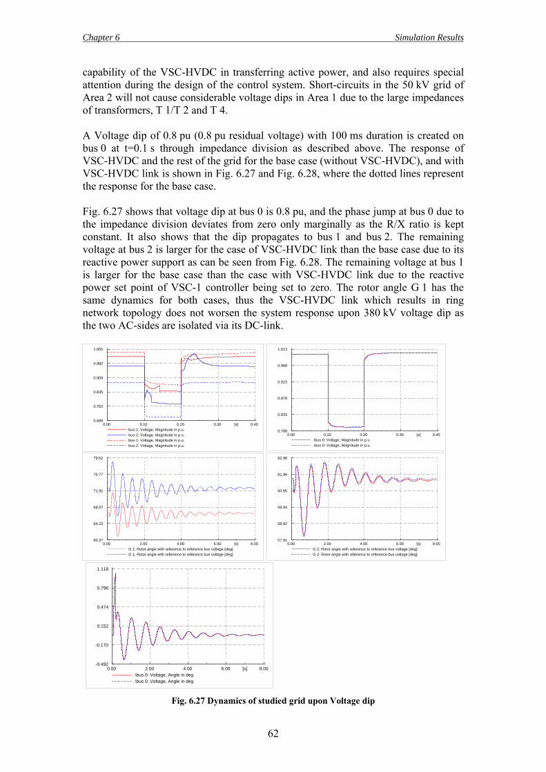
Chapter 6 Simulation Results
62
capability of the VSC-HVDC in transferring active power, and also requires special attention during the design of the control system. Short-circuits in the 50 kV grid of Area 2 will not cause considerable voltage dips in Area 1 due to the large impedances of transformers, T 1/T 2 and T 4. A Voltage dip of 0.8 pu (0.8 pu residual voltage) with 100 ms duration is created on bus 0 at t=0.1 s through impedance division as described above. The response of VSC-HVDC and the rest of the grid for the base case (without VSC-HVDC), and with VSC-HVDC link is shown in Fig. 6.27 and Fig. 6.28, where the dotted lines represent the response for the base case. Fig. 6.27 shows that voltage dip at bus 0 is 0.8 pu, and the phase jump at bus 0 due to the impedance division deviates from zero only marginally as the R/X ratio is kept constant. It also shows that the dip propagates to bus 1 and bus 2. The remaining voltage at bus 2 is larger for the case of VSC-HVDC link than the base case due to its reactive power support as can be seen from Fig. 6.28. The remaining voltage at bus 1 is larger for the base case than the case with VSC-HVDC link due to the reactive power set point of VSC-1 controller being set to zero. The rotor angle G 1 has the same dynamics for both cases, thus the VSC-HVDC link which results in ring network topology does not worsen the system response upon 380 kV voltage dip as the two AC-sides are isolated via its DC-link.
0.400.300.200.100.00 [s]
1.055
0.982
0.909
0.835
0.762
0.689
bus-1: Voltage, Magnitude in p.u.bus-2: Voltage, Magnitude in p.u.bus-1: Voltage, Magnitude in p.u.bus-2: Voltage, Magnitude in p.u.
0.400.300.200.100.00 [s]
1.013
0.968
0.923
0.878
0.833
0.788
.\bus 0: Voltage, Magnitude in p.u.
.\bus 0: Voltage, Magnitude in p.u.
8.006.004.002.000.00 [s]
79.62
75.77
71.92
68.07
64.22
60.37
G 1: Rotor angle with reference to reference bus voltage [deg]G 1: Rotor angle with reference to reference bus voltage [deg]
8.006.004.002.000.00 [s]
62.98
61.96
60.95
59.94
58.92
57.91
G 2: Rotor angle with reference to reference bus voltage [deg]G 2: Rotor angle with reference to reference bus voltage [deg]
8.006.004.002.000.00 [s]
1.118
0.796
0.474
0.152
-0.170
-0.492
.\bus 0: Voltage, Angle in deg
.\bus 0: Voltage, Angle in deg
Fig. 6.27 Dynamics of studied grid upon Voltage dip
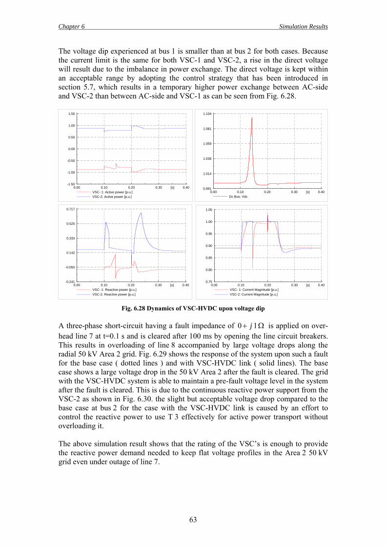
Chapter 6 Simulation Results
63
The voltage dip experienced at bus 1 is smaller than at bus 2 for both cases. Because the current limit is the same for both VSC-1 and VSC-2, a rise in the direct voltage will result due to the imbalance in power exchange. The direct voltage is kept within an acceptable range by adopting the control strategy that has been introduced in section 5.7, which results in a temporary higher power exchange between AC-side and VSC-2 than between AC-side and VSC-1 as can be seen from Fig. 6.28.
0.400.300.200.100.00 [s]
1.104
1.081
1.059
1.036
1.014
0.991
Dc Bus: Vdc
0.400.300.200.100.00 [s]
1.50
1.00
0.50
0.00
-0.50
-1.00
-1.50
VSC- 1: Active power [p.u.]VSC-2: Active power [p.u.]
0.400.300.200.100.00 [s]
0.717
0.525
0.333
0.142
-0.050
-0.241
VSC- 1: Reactive power [p.u.]VSC-2: Reactive power [p.u.]
0.400.300.200.100.00 [s]
1.05
1.00
0.95
0.90
0.85
0.80
0.75
VSC- 1: Current Magnitude [p.u.]VSC-2: Current Magnitude [p.u.]
Fig. 6.28 Dynamics of VSC-HVDC upon voltage dip A three-phase short-circuit having a fault impedance of 0 1j+ Ω is applied on over-head line 7 at t=0.1 s and is cleared after 100 ms by opening the line circuit breakers. This results in overloading of line 8 accompanied by large voltage drops along the radial 50 kV Area 2 grid. Fig. 6.29 shows the response of the system upon such a fault for the base case ( dotted lines ) and with VSC-HVDC link ( solid lines). The base case shows a large voltage drop in the 50 kV Area 2 after the fault is cleared. The grid with the VSC-HVDC system is able to maintain a pre-fault voltage level in the system after the fault is cleared. This is due to the continuous reactive power support from the VSC-2 as shown in Fig. 6.30. the slight but acceptable voltage drop compared to the base case at bus 2 for the case with the VSC-HVDC link is caused by an effort to control the reactive power to use T 3 effectively for active power transport without overloading it. The above simulation result shows that the rating of the VSC’s is enough to provide the reactive power demand needed to keep flat voltage profiles in the Area 2 50 kV grid even under outage of line 7.
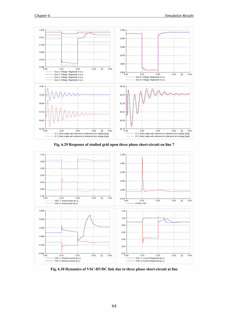
Chapter 6 Simulation Results
64
0.400.300.200.100.00 [s]
1.076
0.917
0.759
0.600
0.442
0.283
bus-1: Voltage, Magnitude in p.u.bus-2: Voltage, Magnitude in p.u.bus-1: Voltage, Magnitude in p.u.bus-2: Voltage, Magnitude in p.u.
0.400.300.200.100.00 [s]
1.004
0.994
0.985
0.975
0.965
0.956
.\bus 0: Voltage, Magnitude in p.u.
.\bus 0: Voltage, Magnitude in p.u.
8.006.004.002.000.00 [s]
74.87
72.35
69.84
67.33
64.81
62.30
G 1: Rotor angle with reference to reference bus voltage [deg]G 1: Rotor angle with reference to reference bus voltage [deg]
8.006.004.002.000.00 [s]
62.05
61.67
61.29
60.91
60.53
60.14
G 2: Rotor angle with reference to reference bus voltage [deg]G 2: Rotor angle with reference to reference bus voltage [deg]
Fig. 6.29 Response of studied grid upon three phase short-circuit on line 7
0.400.300.200.100.00 [s]
1.106
1.081
1.055
1.030
1.005
0.979
Dc Bus: Vdc
0.400.300.200.100.00 [s]
1.20
0.80
0.40
0.00
-0.40
-0.80
-1.20
VSC- 1: Active power [p.u.]VSC-2: Active power [p.u.]
0.400.300.200.100.00 [s]
0.800
0.560
0.320
0.080
-0.160
-0.400
VSC- 1: Reactive power [p.u.]VSC-2: Reactive power [p.u.]
0.400.300.200.100.00 [s]
1.20
1.00
0.80
0.60
0.40
0.20
0.00
VSC- 1: Current Magnitude [p.u.]VSC-2: Current Magnitude [p.u.]
Fig. 6.30 Dynamics of VSC-HVDC link due to three phase short-circuit at line
65
Chapter 7 Conclusions and Further Research 7.1 Conclusions and Recommendations The recent development in semiconductor and control equipment has made HVDC transmission based on voltage-source converter (VSC-HVDC) feasible. VSC-HVDC has numerous advantages such as a controllable short-circuit current contribution, the rapid and independent control of active and reactive power, and good power quality. With these advantages VSC-HVDC can likely be used to solve constraints in sub-transmission and distribution networks. The technical characteristics of a coupling between two sub-transmission systems on 50 kV level through VSC-HVDC are investigated. The main objective of the VSC-HVDC link is to mitigate network constraints in one of these networks. Area 1 is a greenhouse area having a large penetration level of CHP-plants, and Area 2 feeds a 50 kV grid that is expected to be constrained in the nearby future. The dynamic reactive power support capability of the VSC-HVDC and the available distributed generation in Area 1 are used to solve the constraints in Area 2. An adequate model of a VSC-HVDC taking into account the gird constraints, identified through extensive load flow and N-1 outage calculations, is presented. The vector control system of the converters valid for balanced RMS simulations has been established and the performance of the VSC-HVDC under idealized network conditions is investigated. From simulation results, it can be concluded that the system response is fast, and the active and reactive power can be controlled independently and bi-directionally. Comprehensive scenarios have been investigated to assess the performance of the VSC-HVDC in mitigating the network constraints and postpone major reinforcements of the network infrastructure. The impact of the VSC-HVDC on major power system planning issues; interaction with other installed units (e.g. wind generators), protection scheme, impact on network topology are investigated. Based on the work performed for this thesis, the following conclusions can be drawn;
• The involved physical constraints, static voltage sensitivity analysis and load growth trends revealed that the VSC-HVDC model shall be of back to back topology placed in Area 2 with PCCs at bus 2 and bus 1.
• The rating of the VSC-HVDC converters, 45 MVA is found to be
sufficient to transfer the planned 40 MW, and have enough reactive power capacity together with the AC filter banks to deal with the worst case N-1 outage voltage drops.
Chapter 7 Conclusions and Further Research
66
• The performance of the converter controllers under steady state and various disturbances has been found to be in agreement with other research works.
• It is not required to model the distribution grid in Area 1 in detail, i.e. the
aggregated model of the distribution grid is valid for the purpose of the planning studies presented in this thesis.
• The steady-state and dynamics of rotor angles of the large synchronous
generators G 2/G 3 is affected only marginally due to the introduction of VSC-HVDC. Moreover, the transmission grid power flows change only by a relatively small proportion, 3 % because of the VSC-HVDC instigate power flow changes.
• The ability of the distribution grid to remain in synchronism with the rest
of the grid is improved by the VSC-HVDC link to some extent.
• The interaction of the largest wind unit installed at line 2/line 3 with the VSC-HVDC is not significant. This may be attributed to the low i.e. 15 % penetration level of the wind power in the 50 kV Area 2 grid.
• The maximum relative increase in short-circuit current in the 50 kV Area 2
grid due to the VSC-HVDC is found to be 13 %. For grid operators, an increases of 13 % for short-circuit current levels in the range of 4 kA is acceptable. Thus, there is no need to upgrade existing circuit breakers and revise the protection scheme of the existing grid.
• The response of the network to deep voltage dips in the 380 kV network is
not significantly affected by the VSC-HVDC link. The performance of the VSC-HVDC deteriorates under such deep voltage dip. However, the probability of occurrence of such dips is rare.
• Technically the VSC-HVDC is found to be an innovative and sufficient
solution to mitigate the network constraints described in this thesis. The author believes that this is the first attempt made to give a comprehensive investigation of the use of VSC-HVDC to mitigate network constraints in a meshed network than on idealized network conditions. 7.2 Further Research To further evaluate the application of a VSC-HVDC for alleviating network constraints in the studied grid, a more detailed assessment using an appropriate EMT model, taking into account all possible grid operating conditions, need to be made. Some of the possible future works could be listed as follows:
• Improvement in the control system to deal with unbalanced faults and harmonic elimination. This can be achieved by dealing with the negative and positive sequence currents separately. This will help to supply generate
Chapter 7 Conclusions and Further Research
67
balanced currents and voltages in the case of unbalanced faults which may avoid unnecessary tripping of the DC-link.
• Further optimization of the controller parameters with respect to control
system stability and dynamic responses. This will help to increase the availability of the VSC-HVDC link.
• A little insight to the associated investments is given in this thesis. A more
detailed analysis and comparison with other solution may make management decision easier.
• Extending the load growth and other studied scenarios to a more detail level
may reveal other benefits or disadvantage of the VSC-HVDC solution.
68
Appendix A Space vectors In three phase systems, it can often be assumed that the instantaneous sum of the components e.g. voltages add up to zero 0a b cv v v t+ + = ∀ (A.1) That is, a zero sequence component is assumed not to exist. This removes one degree of freedom, since on of the phase voltages, e.g., cv always can be expressed in the other two: ( )c a bv v v= − + . Therefore it is possible to describe the three phase system as an equivalent two phase system, with two perpendicular axes, denoted as α andβ . It is convenient to consider these axes as the real and imaginary axes in a complex plane. With the complex two phase representation v v jvαβ α β= + , the three phase/two phase transformation is given by normalized Clark transformation also called power invariant Clark transformation as:
2 /3 4 /32 ( )3
j ja b cv jv v e v e vπ π
α β= + = + +αβv (A.2)
where vαβ indicated the stationary reference frame. A set of positive sequence
components, with the α -phase quantity given by 1 1cos( ),a ev V d dtθ φ θ ω∧
= + = ,
where the peak value V∧
and the phase angle φ can be assumed constant in steady state, resulting in the space vector
1( )jV e θ φ∧
+=αβv (A.3) This vector rotates counterclockwise with the angular synchronous frequency eω . A negative sequence waveform gives a similar expression, but with a minus sign in the exponent. Other three phase quantities particularly currents can be transformed in similar way. Fig.A.1 shows voltage and currents components in αβ -frame and dq -frame. It is often reasonable to express the space vector in some other coordinate system than the stationary αβ reference frame. The transformation from the stationary to a general coordinate system is given by -jθg
g αβv = v e (A.4) where gθ is the phase angle of the general reference frame with respect to the real axis of the stationary frame. If the general coordinate system rotates with the same
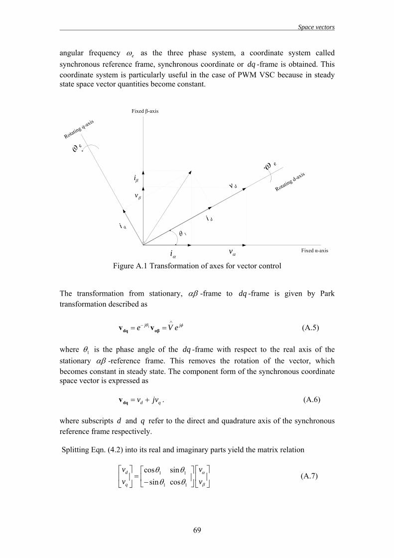
Space vectors
69
angular frequency eω as the three phase system, a coordinate system called synchronous reference frame, synchronous coordinate or dq -frame is obtained. This coordinate system is particularly useful in the case of PWM VSC because in steady state space vector quantities become constant.
Rotating d-axis
Rotating q-axis
Fixed α-axis
Fixed β-axis
diqi
dv
vαiα
iβ
vβ
1θ
eω
eω
Figure A.1 Transformation of axes for vector control
The transformation from stationary, αβ -frame to dq -frame is given by Park transformation described as
1j je V eθ φ∧
−= =dq αβv v (A.5) where 1θ is the phase angle of the dq -frame with respect to the real axis of the stationary αβ -reference frame. This removes the rotation of the vector, which becomes constant in steady state. The component form of the synchronous coordinate space vector is expressed as d qv jv= +dqv . (A.6) where subscripts d and q refer to the direct and quadrature axis of the synchronous reference frame respectively. Splitting Eqn. (4.2) into its real and imaginary parts yield the matrix relation
1 1
1 1
cos sinsin cos
d
q
v vv v
α
β
θ θθ θ
⎡ ⎤ ⎡ ⎤⎡ ⎤=⎢ ⎥ ⎢ ⎥⎢ ⎥−⎣ ⎦ ⎣ ⎦⎣ ⎦
(A.7)
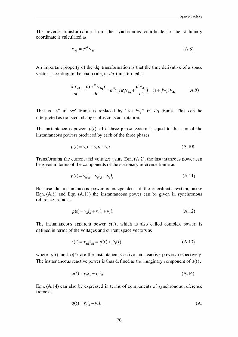
Space vectors
70
The reverse transformation from the synchronous coordinate to the stationary coordinate is calculated as 1je θ=αβ dqv v (A.8) An important property of the dq transformation is that the time derivative of a space vector, according to the chain rule, is dq transformed as
1
1( )
( ) ( )j
je e
d d e de jw s jw
dt dt dt
θθ= = + = +αβ dq dq
dq dq
v v vv v (A.9)
That is “s” in αβ -frame is replaced by “ es jw+ ” in dq -frame. This can be interpreted as transient changes plus constant rotation. The instantaneous power ( )p t of a three phase system is equal to the sum of the instantaneous powers produced by each of the three phases ( ) a a b b c cp t v i v i v i= + + (A.10) Transforming the current and voltages using Eqn. (A.2), the instantaneous power can be given in terms of the components of the stationary reference frame as ( ) o op t v i v i v iα α β β= + + (A.11) Because the instantaneous power is independent of the coordinate system, using Eqn. (A.8) and Eqn. (A.11) the instantaneous power can be given in synchronous reference frame as ( ) d d q q o op t v i v i v i= + + (A.12) The instantaneous apparent power ( )s t , which is also called complex power, is defined in terms of the voltages and current space vectors as ( ) ( ) ( )s t p t jq t= = +αβ αβv i (A.13) where ( )p t and ( )q t are the instantaneous active and reactive powers respectively. The instantaneous reactive power is thus defined as the imaginary component of ( )s t . ( )q t v i v iβ α α β= − (A.14) Eqn. (A.14) can also be expressed in terms of components of synchronous reference frame as ( ) q d d qq t v i v i= − (A.
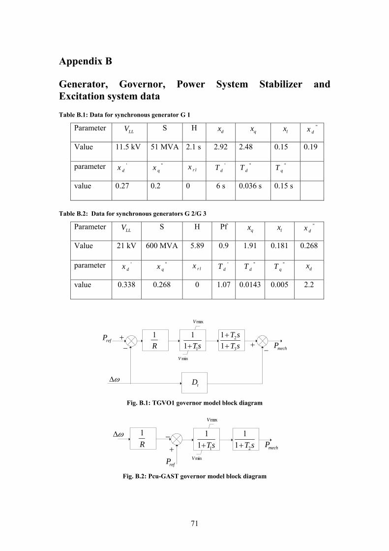
71
Appendix B Generator, Governor, Power System Stabilizer and Excitation system data Table B.1: Data for synchronous generator G 1
Parameter LLV S H dx qx lx ''dx
Value 11.5 kV 51 MVA 2.1 s 2.92 2.48 0.15 0.19
parameter 'dx ''
qx r lx 'dT ''
dT ''qT
value 0.27 0.2 0 6 s 0.036 s 0.15 s
Table B.2: Data for synchronous generators G 2/G 3
Parameter LLV S H Pf qx lx ''dx
Value 21 kV 600 MVA 5.89 0.9 1.91 0.181 0.268
parameter 'dx ''
qx r lx 'dT ''
dT ''qT dx
value 0.338 0.268 0 1.07 0.0143 0.005 2.2
−+
+2
3
11
T sT s
++1
11 T s+
1R
tDωΔ
− mechPrefP
maxV
minV
Fig. B.1: TGVO1 governor model block diagram
−
+ 2
11 T s+1
11 Ts+
ωΔ
refP
maxV
minV
1R mechP
Fig. B.2: Pcu-GAST governor model block diagram
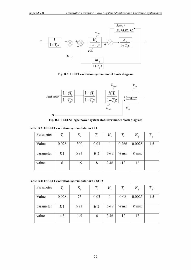
Appendix B Generator, Governor, Power System Stabilizer and Excitation system data
72
−+
+ 1e
e
KT s+1
a
a
KT s+
11 rT s+
−
( )
1, 1, 2, 2fdSe e
E Se E SemaxV
minV
−+
1f
f
sKT s+
refU
U
Fig. B.3: IEET1 excitation system model block diagram
5
61sKTT s+
u
.Accel power
maxsL
minsL
3
4
11
sTT s
++
1
2
11
sTT s++ limiter
cuV
clV
Fig. B.4: IEEEST type power system stabilizer model block diagram
Table B.3: IEEET1 excitation system data for G 1
Parameter rT aK aT eK eT fK fT
Value 0.028 300 0.03 1 0.266 0.0025 1.5
parameter 1E 1S e 2E 2S e
minVr maxVr
value 6 1.5 8 2.46 -12 12
Table B.4: IEEET1 excitation system data for G 2/G 2
Parameter rT aK aT eK eT fK fT
Value 0.028 75 0.03 1 0.08 0.0025 1.5
parameter 1E 1S e 2E 2S e
minVr maxVr
value 4.5 1.5 6 2.46 -12 12
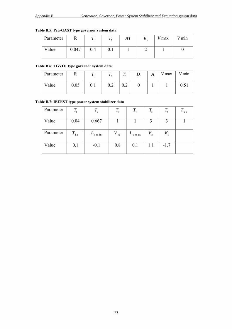
Appendix B Generator, Governor, Power System Stabilizer and Excitation system data
73
Table B.5: Pcu-GAST type governor system data
Parameter R 1T 2T AT tK maxV minV
Value 0.047 0.4 0.1 1 2 1 0
Table B.6: TGVO1 type governor system data
Parameter R 1T 2T 3T tD tA maxV minV
Value 0.05 0.1 0.2 0.2 0 1 1 0.51
Table B.7: IEEEST type power system stabilizer data
Parameter 1T 2T 3T 4T 5T 6T d uT
Value 0.04 0.667 1 1 3 3 1
Parameter 1 uT m insL c lV m a xsL
cuV sK
Value 0.1 -0.1 0.8 0.1 1.1 -1.7
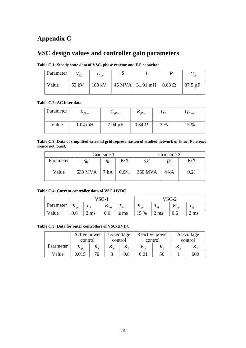
74
Appendix C
VSC design values and controller gain parameters Table C.1: Steady state data of VSC, phase reactor and DC capacitor
Parameter LLV dcU S L R dcC
Value 52 kV 100 kV 45 MVA 31.91 mH 0.83 Ω 37.5 µF
Table C.2: AC filter data
Parameter filterL filterC filterR fQ filterQ
Value 1.04 mH 7.94 µF 0.34 Ω 3 % 15 %
Table C.3: Data of simplified external grid representation of studied network of Error! Reference source not found.
Grid side 1 Grid side 2 Parameter ''Sk ''Ik R/X ''Sk ''Ik R/X
Value 630 MVA 7 kA 0.041 360 MVA 4 kA 0.21
Table C.4: Current controller data of VSC-HVDC
VSC-1 VSC-2 Parameter
pdK idT pqK iqT pdK idT pqK iqT
Value 0.6 2 ms 0.6 2 ms 15 % 2 ms 0.6 2 ms
Table C.5: Data for outer controllers of VSC-HVDC
Active power control
Dc-voltage control
Reactive power control
Ac-voltage control
Parameter pK IK pK
IK pK IK pK
IK Value 0.015 70 8 0.8 0.01 50 1 600
75
References [1] "DIgSILENT PowerFactory/Reference document/Synchronous machine
modelling", [Available from: http://www.digsilent.de/], Germany, 2007 [2] Reza, M., "Stability analysis of transmission systems with high penetration of
distributed generation ", Ph.D. dissertation, Delft University of Technology, Delft, The Netherlands, 2006
[3] Ishchenko, A., "Dynamics and stability of Distribution Networks with Dispersed Generation", Ph.D. dissertation, Techinical University of Eindhoven, Eindhoven, The Netherlands, 2008
[4] Shire, T.W. "Power flow controller as an innovative solution to network constraints ", Internal document, STEDIN, Rotterdam, The Netherlands, 2008
[5] M.H.Haque, "Power flow control and voltage stability limit:regulating transformer versus UPFC", IEE Proc-Gener.Transm.Distrib, Vol. 151, may 2004
[6] Fischer de Toledo, P., "Feasibility of HVDC for city infeed", Licentiate Thesis, Royal institute of Technology, Stockholm, 2003
[7] Verboomen, J., "Optimisation of transmission systems by use of phase shifting transformers", Ph.D. dissertation, Delft University of Technology, Delft, The Netherlands, 2008
[8] Bajracharaya, C., "Control of VSC-HVDC for wind power", M.Sc. thesis, Norwegian University of Science and Technology, June 2008
[9] Du, C., "The control of VSC-HVDC and its use for large industrial power system", Licentiate thesis, Chalmers University of Technology, Göteborg, Sweden, April 2003
[10] Pan, J., et al. VSC-HVDC control and application in meshed networks in Proc. 2008 IEEE PES general meeting 2008. Pittsburgh, Pennsylvania.
[11] Mohan, N., T.M. Underland, and W.P. Robbins, eds. Power Electronics-converter, design and application. 2 ed. 1995, John Wiley.
[12] Xu, Z., "Advanced semiconductor device and topology for high power current source converters", Ph.D. dissertation, Virginia Polytechnic Institute and State University, Blackburg, Virginia, 2003
[13] Norrga, S., et al., Voltage source converters in transmission application, in Proc. 2008 IEEE Power Electronics Specialists Conference. 2008: Rhodes, Greece.
[14] D.Hansen, A., et al. "Dynamic wind turbine models in power system simulation tool DIgSILENT", Riso National Labratory, Technical University of Denmark Roskilde, Denmark, 2007
[15] Pollanen, R., "Converter-flux-based current control of voltage source PWM rectifier analysis and implementation", Ph.D. dissertation, Acta University, Lappeenrantaensis, Finland, December 2003
[16] Abbay, C. "Protection coordination planning with distributed generation", CETC Varennes-Energy technology and program sector, Canada, June 2007
[17] Morren, J., "Grid support by power electronic converters of distributed generation units", Ph.D. dissertation, Delft University of Technology, Delft, The Netherlands, 2006
76
[18] Du, C. and E. Agneholm. Investigation of Frequency/Ac voltage control for inverter station of VSC-HVDC. in Proc. 32nd IEEE Annual Conference on Industrial Electronics. 2007. Paris, France.
[19] Bohn, C. and D.P. Atherton, "Analysis package comparing PID ani-windup strategies", IEEE Control Systems Magazine, Vol. 15(2): p. 34-40, April 1995
[20] Harnefors, L. Control of VSC-HVDC Transmissions. in Proc. 2008 IEEE Power Electronics Specialists Conference. 2008. Rhodes, Greece.
[21] Xu, L., B.R. Anderson, and P. Cartwright, "VSC-Transmission operating under unbalanced AC conditions-Analysis and Control Design", IEEE Transactions on Power Delivery, Vol. 20(1), January 2005
[22] Bjorklund, P.-E., K. Srivastava, and W. Quaintance. HVDC Light modeling for dynamic performance analysis. in Proc. IEEE Power Systems Conference and Exposition. 2006. Atlanta, Georgia.
[23] Khan, A.A., "A simple method for tracing PV curves of a radial transmission line ", Proceedings of World Academy of Science, Engineering and Technology (PWASET), Vol. 27, February 2008
[24] Jiang-Häfner, Y., M. Hyttinen, and B. Pääjärvi. On the short circuit current contribution of HVDC light. in Proc. IEEE/PES Transmission and Distribution Conference and Exhibition; Asia Pacific. 2002. Yokohama, Japan.
[25] "HVDC Light system interactive tutorial", [Available from: www.abb.com/hvdc], [26] Johansson, S.G., et al. Power system stability benefits with VSC dc-transmission
systems in Proc. CIGRE Session 2004. 2004. Paris, France. [27] "Wind Farm integration in British Columbia - Stages 1 & 2: Planning and
interconnection Criteria ", Report number 2005-10988-2.R01.4, issued by ABB Electric Systems Consulting, March 2005
[28] Lasseter, R., K. Tomsovic, and P. Piagi. "Scenarios for distributed technology applications with Steady state and dynamic models of loads and micro-sources", Consortium for Electrical Reliability Technology Solutions, Power system Engineering Research center, University of Wisconsin, Madison, April 2000
[29] Slootweg, J.G., "Wind Power Modelling and Impact on Power System Dynamics", Ph.D. dissertation, Delft University of Technology, Delft, The Netherlands, 2003
[30] Coster, E.J., J.M.A. Myrzik, and W.L. Kling. Grid Interaction of MV-connected CHP-Plants during Disturbances. in IEEE PES General Meeting. 2009. Calgary, Canada